Test (2009) 18: 392–413DOI 10.1007/s11749-008-0108-8

O R I G I NA L PA P E R

Semi-parametric second-order reduced-bias highquantile estimation

Frederico Caeiro · M. Ivette Gomes

Received: 26 May 2007 / Accepted: 27 February 2008 / Published online: 26 March 2008© Sociedad de Estadística e Investigación Operativa 2008

Abstract In many areas of application, like, for instance, Climatology, Hydrology,Insurance, Finance, and Statistical Quality Control, a typical requirement is to esti-mate a high quantile of probability 1 − p, a value high enough so that the chance ofan exceedance of that value is equal to p, small. The semi-parametric estimation ofhigh quantiles depends not only on the estimation of the tail index or extreme valueindex γ , the primary parameter of extreme events, but also on the adequate estimationof a scale first order parameter. Recently, apart from new classes of reduced-bias esti-mators for γ > 0, new classes of the scale first order parameter have been introducedin the literature. Their use in quantile estimation enables us to introduce new classesof asymptotically unbiased high quantiles’ estimators, with the same asymptotic vari-ance as the (biased) “classical” estimator. The asymptotic distributional properties ofthe proposed classes of estimators are derived and the estimators are compared withalternative ones, not only asymptotically, but also for finite samples through MonteCarlo techniques. An application to the log-exchange rates of the Euro against theSterling Pound is also provided.

Keywords Heavy tails · High quantiles · Semi-parametric estimation · Statistics ofextremes

Mathematics Subject Classification (2000) Primary 62G32 · 62E20 ·Secondary 65C05

F. Caeiro (�)New University of Lisbon and CMA, Lisbon, Portugale-mail: fac@fct.unl.pt

M.I. GomesUniversity of Lisbon, DEIO, CEAUL and FCUL, Lisbon, Portugale-mail: ivette.gomes@fc.ul.pt

Semi-parametric second-order reduced-bias high quantile estimation 393

1 Introduction and preliminaries

A model F is said to be heavy-tailed, with a tail index γ (> 0), if the tail functionF := 1 − F ∈ RV−1/γ , where for any real α, RVα denotes the class of regularlyvarying functions with index of regular variation equal to α, i.e., non-negative mea-surable functions g such that, for all x > 0, g(tx)/g(t) → xα , as t → ∞ (Gnedenko1943). Let us denote U(t) := F←(1 − 1/t) = inf{x : F(x) ≥ 1 − 1/t}. Then, we mayequivalently say that F is heavy-tailed if and only if U ∈ RVγ (de Haan 1970), i.e.,

limt→∞

U(tx)

U(t)= xγ , for any x > 0. (1)

For small values of p, we want to estimate χ1−p , a value such that F(χ1−p) = 1 −p,a typical parameter in the most diversified areas of application, among which wemention climatology, hydrology, economics, insurance, and finance. More specifi-cally, we want to extrapolate beyond the sample, i.e., we want to estimate

χ1−p = U(1/p), p = pn → 0, npn → K as n → ∞, K ∈ [0,1], (2)

and we shall assume to be working in Hall’s class of models (Hall 1982) where thereexist γ > 0, ρ < 0, C > 0, and β �= 0 such that

U(t) = Ctγ(1 + γβtρ/ρ + o

(tρ

)). (3)

For some details in the paper we shall refer to a sub-class of Hall’s class such that

U(t) = Ctγ(1 + γβtρ/ρ + β ′t2ρ + o

(t2ρ

)), (4)

i.e., relatively to Hall’s class we merely make explicit a third order term β ′t2ρ , β ′ �= 0.Such a class contains most of the heavy-tailed models important in applications, likethe Fréchet, the Generalized Pareto, and the Student’s-t . For quantile estimation in aslightly more general class than the one in (4), we refer Caeiro and Gomes (2008).

We are going to base inference on the largest k order statistics (o.s.), and as usual insemi-parametric estimation of parameters of extreme events, we shall assume that k

is an intermediate sequence of integers in [1, n[, i.e.,

k = kn → ∞, k/n → 0, n → ∞. (5)

Since, from (2) and (3), χ1−p = U(1/p) ∼ Cp−γ , as p → 0, an obvious estimatorof χ1−p is Cp−γ , with C and γ any consistent estimators of C and γ , respectively.Given a sample (X1,X2, . . . ,Xn), let us denote Xi:n, 1 ≤ i ≤ n, the set of associatedascending order statistics. Denoting Y a standard Pareto model, i.e., a model such thatFY (y) = 1 − 1/y, y > 1, the use of the universal uniform transformation enables us

to write Xn−k:nd= U(Yn−k:n). Next, with the notation Un

p∼ Vn if and only if Un/Vn

converges in probability towards 1, since Yn−k:np∼ (n/k) for intermediate k and (3)

holds, we get Xn−k:np∼ CY

γ

n−k:np∼ C(n/k)γ , as n → ∞. Consequently, an obvious

394 F. Caeiro, M.I. Gomes

estimator of C, proposed by Hall (1982), is

Cγ (k) := Xn−k:n(

k

n

)γ

, (6)

and

Q(p)

γ(k) = Cp−γ = Xn−k:n

(k

np

)γ

(7)

is the obvious quantile-estimator at the level p (Weissman 1978).For heavy tails, the classical tail index estimator, usually the one which is plugged

in (7), for a semi-parametric quantile estimation, is the Hill estimator γ = γ (k) =:H(k) (Hill 1975) with the functional expression

H(k) := 1

k

k∑

i=1

Vik = 1

k

k∑

i=1

Ui, (8)

where Vik := lnXn−i+1:n − lnXn−k:n, 1 ≤ i ≤ k < n, are the log-excesses, and

Ui := i (lnXn−i+1:n − lnXn−i:n) , 1 ≤ i ≤ k < n, (9)

are the scaled log-spacings. We thus get the so-called classical quantile estimator,based on the Hill tail index estimator H , with the obvious notation, Q

(p)H (k).

In order to derive the asymptotic non-degenerate behavior of semi-parametric es-timators of extreme events’ parameters, we need more than the first order conditionin (1). A typical condition for heavy-tailed models, which holds for the models in (3),with

A(t) = γβtρ, γ > 0, β �= 0, ρ < 0, (10)

is the condition,

limt→∞

U(tx)U(t)

− xγ

A(t)= xγ xρ − 1

ρ, (11)

for all x > 0, where A is a function of constant sign near infinity (positive or nega-tive), and ρ ≤ 0 is the shape second order parameter.

Under the second order framework in (11), and for intermediate k, i.e., when-ever (5) holds, we may guarantee the asymptotic normality of the Hill estimator H(k),for an adequate k. Indeed, we may write (de Haan and Peng 1998),

H(k)d= γ + γ Zk/

√k + (

A(n/k)/(1 − ρ))(

1 + op(1)), (12)

with Zk = √k(

∑ki=1 Ei/k − 1) asymptotically standard normal, {Ei} i.i.d. standard

exponential r.v.’s. Consequently, if we choose k such that√

kA(n/k) → λ �= 0, fi-nite, as n → ∞,

√k(H(k) − γ ) is asymptotically normal, with variance equal to γ 2

and a non-null bias given by λ/(1 − ρ). Most of the times, this type of estimates ex-hibits a strong bias for moderate k and sample paths with very short stability regions

Semi-parametric second-order reduced-bias high quantile estimation 395

around the target value γ . This has recently led researchers to consider the possibilityof dealing with the bias term in an appropriate way, building new estimators, γ

R(k)

say, the so-called second order reduced-bias estimators discussed by Peng (1998),Beirlant et al. (1999), Feuerverger and Hall (1999), Gomes et al. (2000), among oth-ers. Then, for k intermediate, i.e., such that (5) holds, and under the second orderframework in (11), we may write, with ZR

k an asymptotically standard normal r.v.,

γR(k)

d= γ + γ σR

ZRk /

√k + op

(A(n/k)

), (13)

where σR

> 0 and A is again the function in (11). Consequently, the sequence ofr.v.’s,

√k(γ

R(k) − γ ) is asymptotically normal with variance equal to (γ σ

R)2 and

a null mean value even when√

k A(n/k) → λ �= 0, finite, as n → ∞, possibly atthe expense of an asymptotic variance γ 2σ 2

R> γ 2. Gomes and Figueiredo (2006)

suggest the use, in (7), of reduced-bias tail index estimators, like the ones in Gomesand Martins (2001, 2002) and Gomes et al. (2004), all with σ

R> 1 in (13), being

then able to reduce also the dominant component of the classical quantile estimator’sasymptotic bias.

More recently, Caeiro et al. (2005), Gomes et al. (2007a, 2007b) consider newclasses of tail index estimators, for which (13) holds with σ

R= 1 at least for values

k such that√

k A(n/k) → λ, finite. These classes are dependent on (β, ρ), an ad-equate consistent estimator of the vector of second order parameters (β,ρ) in (10).The influence of these tail index estimators in quantile estimation has been studiedby Gomes and Pestana (2007) and Beirlant et al. (2006).

Also recently, new estimators of C have been proposed in Caeiro (2006), where,instead of Xn−k:n alone, a spacing Xn−[θk]:n − Xn−k:n, 0 < θ < 1, is considered.More specifically, we may replace Cγ (k) in (6) by

CγR(k; θ) := Xn−[θk]:n − Xn−k:n

θ−γR − 1

(k

n

)γR

, (14)

where θ ∈]0,1[ is a tuning parameter and γR

≡ γR(k) is a second order reduced-bias

tail index estimator. Similarly to the way developed by Caeiro et al. (2005) for thetail index estimation, Caeiro (2006) has worked out the main dominant componentof the asymptotic bias of Cγ

R(k; θ) in (14). With the parameterization A(t) = γβtρ ,

already given in (10), such a component is given by C × Bθ (γ, ρ,β), where

Bθ (γ, ρ,β) = θ−(γ+ρ) − 1

θ−γ − 1× γβ(n/k)ρ

ρ.

It is thus sensible to consider the semi-parametric C-estimator,

CγR(k; θ) := Xn−[θk]:n − Xn−k:n

θ−γR − 1

(k

n

)γR × (

1 − Bθ (γR, ρ, β)

). (15)

396 F. Caeiro, M.I. Gomes

We shall here consider the associated quantile estimator,

Q(p)

γR

(k; θ) ≡ Q(p)

γR

,ρ,β(k; θ) := Xn−[θk]:n − Xn−k:n

θ−γR − 1

(k

np

)γR × (

1 − Bθ (γR, ρ, β)

).

(16)

For adequate consistent estimators β and ρ of the second order parameters β

and ρ, respectively, we shall restrict our attention to the second order reduced-biastail index estimator introduced in Caeiro et al. (2005),

H(k) ≡ Hβ,ρ

(k) := H(k)

(1 − β

(n

k

)ρ

/(1 − ρ)

). (17)

After a brief sketch on the estimation of the second order parameters, in Sect. 2,we provide, in Sect. 3, details on the reduced-bias estimators of γ and C to be usedfor quantile estimation. Section 4 is devoted to the asymptotic behavior of quantileestimators and Sect. 5, to their finite sample properties. In Sect. 6, we study the ro-bustness of the proposed class of quantile estimators to underlying heavy-tailed mod-els that may be no longer supported by the developed theory. Finally, in Sect. 7, weprovide an illustration, for data from the field of finance.

2 Estimation of second order parameters

The reduced-bias estimators in (15), (16), and (17) require the estimation of the sec-ond order parameters ρ and β in (10). Such an estimation will now be briefly dis-cussed.

2.1 Estimators of the shape second order parameter ρ

We shall consider here particular members of the class of estimators of the secondorder parameter ρ proposed by Fraga Alves et al. (2003). Such a class of estima-tors may be parameterized by a tuning parameter τ ∈ R (as detected by Caeiro andGomes 2006, who use the same type of statistics for the estimation of the scalesecond order parameter β). Denoting M

(j)n (k) the j -moment of the log-excesses,

M(j)n (k) := 1

k

∑ki=1 (lnXn−i+1:n − lnXn−k:n)j , j = 1,2,3, these ρ-estimators de-

pend on the statistics

T (τ)n (k) := (M

(1)n (k))τ − (M

(2)n (k)/2)τ/2

(M(2)n (k)/2)τ/2 − (M

(3)n (k)/6)τ/3

,

where T(τ)n (k) is defined by continuity when τ = 0. These statistics converge towards

the value 3(1 − ρ)/(3 − ρ), independently of the tuning parameter τ , whenever thesecond order condition (11) holds, k is such that (5) holds and

√k A(n/k) → ∞, as

n → ∞. The ρ-estimators considered have the functional expression,

ρ(τ )n (k) := −

∣∣∣3(T (τ)n (k) − 1)/(T (τ)

n (k) − 3)

∣∣∣ . (18)

Semi-parametric second-order reduced-bias high quantile estimation 397

Remark 1 On the basis of simulations, we can say that the ρ-estimators in (18) show,for an appropriate tuning parameter τ , highly stable sample paths as functions of k,the number of top o.s. used, for a wide range of large k-values.

Remark 2 The theoretical and simulated results in Fraga Alves et al. (2003), togetherwith the use of these estimators in different reduced-bias statistics, has led us to advisein practice the estimation of ρ through the estimator in (18), computed at any value

k1 := [n1−ε

], ε > 0, small. (19)

The value k1 in (19) is not necessarily optimal but, for a large class of heavy-tailedmodels, it enables us to guarantee that, with ρ = ρ

(τ )n (k1), (ρ − ρ) = op(1/ lnn), as

n → ∞, a crucial property of the ρ-estimator (see Proposition 3), if we do not want toincrease the asymptotic variance of the r.v. Hβ,ρ , underlying the tail index estimatorH

β,ρin (17). Such a crucial property on ρ can potentially be achieved, without any

restriction in the class of models, if we compute ρ at its optimal level, but the adaptivechoice of such a level is still an open problem. The choice of the tuning parameterτ = 0 for the region ρ ∈ [−1,0) and τ = 1 for the region ρ ∈ (−∞,−1) is a sensibleone. In the simulations of Sect. 5 we have indeed done this. Anyway, we again advisepractitioners not to choose blindly the value of τ in (18). It is sensible to draw a fewsample paths of ρ

(τ )n (k), as functions of k, electing the value of τ which provides

higher stability for large k, by means of any stability criterion. The adequate choiceof τ is much more relevant in practice than the choice of k1.

2.2 Estimators of the scale second order parameter β

For the estimation of β , and with the notations ν(α)n (k) := 1

k

∑ki=1(i/k)α−1,

N(α)n (k) := 1

k

∑ki=1(i/k)α−1Ui , Ui defined in (9), we shall here consider for any

ρ ≡ ρ(τ )n (k) in (18), the estimator developed in Gomes and Martins (2002) and hav-

ing functional expression

βρ (k) :=(

k

n

)ρν

(1−ρ)n (k) N

(1)n (k) − N

(1−ρ)n (k)

ν(1−ρ)n (k) N

(1−ρ)n (k) − N

(1−2ρ)n (k)

. (20)

2.3 Asymptotic behavior

In this paper, we use the same level k1 in (19) both for the estimation of ρ and β

through the estimators in (18) and (20). We now formalize, without proofs, the mostrelevant properties of the second order parameters’ estimators, essentially for theclass of models in (4).

Proposition 1 (Fraga Alves et al. 2003) If the second order condition (11) holds,with ρ ≤ 0, k is a sequence of intermediate integers, i.e., (5) holds, and limn→∞

√k

A(n/k) = ∞, then ρ(τ )n (k) in (18) converges in probability towards ρ, as n → ∞.

Moreover, and now for models in (4), ρ(τ )n (k) − ρ = op(1/ ln(n/k))) for values

398 F. Caeiro, M.I. Gomes

k such that√

kA2(n/k) → λA, finite and non-null, and for values k such that√kA2(n/k) → ∞ for some ε > 0 and k = O(n1−ε).

Proposition 2 (Gomes et al. 2007a) If the second order condition (11) holds withA(t) = γ β tρ , ρ < 0, if (5) holds, and if

√kA(n/k) → ∞, then, with ρ

(τ )n (k)

and βρ (k) given in (18) and (20), respectively, and ρ = ρ(τ )n (k) such that ρ − ρ =

op(1/ lnn), as n → ∞, βρ (k) is consistent for the estimation of β . Moreover,

βρ (k) − βp∼ −β ln(n/k)(ρ − ρ) = op(1).

We shall denote generically ρ any of the estimators in (18), computed at k1 in (19),and β any of the estimators in (20), also computed at the same value k1, for any ε > 0.

3 Reduced-bias estimation of γ and C

We first state the following:

Proposition 3 (Caeiro et al. 2005) If the second order condition (11) holds, ifk = kn is a sequence of intermediate positive integers, i.e., (5) holds, and if√

kA(n/k) → λ, finite and non necessarily null, as n → ∞, then√

k(Hβ,ρ(k) −γ )

d−→n→∞ Normal(0, γ 2). This same limiting behavior holds true if we replace Hβ,ρ

by Hβ,ρ

, provided that ρ − ρ = op(1/ lnn), and we choose β := βρ (k1), with k1 and

βρ (k) given in (19) and (20), respectively. More specifically, and with Zk an asymp-totic standard normal r.v., we can then write

Hβ,ρ

(k)d= γ + γ Zk/

√k + op

(A(n/k)

).

Remark 3 Notice that, contrarily to what happens in Drees’ class of functionals(Drees 1998), where the minimal asymptotic variance of a reduced-bias tail indexestimator is given by (γ (1 −ρ)/ρ)2, we have been here able to obtain a reduced-biastail index estimator with an asymptotic variance equal to γ 2, the asymptotic varianceof Hill’s estimator, the maximum likelihood estimator of γ for a strict Pareto model.

We next present the following results on the asymptotic behavior of intermediateo.s. (de Haan and Ferreira 2006):

Proposition 4 Under the second order framework in (11) and for k such that (5)holds

Xn−k:n/U(n/k)d= 1 + γ Bk/

√k + op

(A(n/k)

), (21)

where Bk is asymptotically standard normal and Cov(Bi,Bj ) = √ij(1 − j/n)/

(j − 1), i < j .

Semi-parametric second-order reduced-bias high quantile estimation 399

Corollary 1 Under the conditions of Proposition 4, and for Hall’s class of modelsin (3),

Xn−k:n/(n/k)γd= C

(1 + γ Bk/

√k + A(n/k)/ρ + op

(A(n/k)

)). (22)

Proof Since Xn−k:n/(n/k)γ = (Xn−k:n/U(n/k)) × (U(n/k)/(n/k)γ ), the resultin (22) follows from Proposition 4 and from (3). �

We may further state the following:

Proposition 5 Let F be a model in Hall’s class, defined in (3). If we consider theHill estimator in (8) and plug it in (6), i.e., if we consider CH (k), further assumingthat

√kA(n/k) → λ, we have

√k(CH (k)/C − 1

)/lnn

d−→n→∞ N

(−λ/((1 − ρ)(1 − 2ρ)

), γ 2/(1 − 2ρ)2).

Proof Since CH (k) = (Xn−k:n/(n/k)γ )(k/n)H(k)−γ , using the result in Corollary 1and applying the delta method to (k/n)H(k)−γ , we get

CH (k)d= C

(1 + γ√

kBk + A(n/k)

ρ

(1 + op(1)

))

× (1 + ln(k/n)

(H(k) − γ

)(1 + op(1)

))

d= C

(1 + ln(k/n)

(H(k) − γ

)(1 + op(1)

) + γ√kBk + A(n/k)

ρ

(1 + op(1)

)),

that is,

√k

lnn

(CH (k) − C

C

)d=

(ln k

lnn− 1

)(γZ

(1)k +

√kA(n/k)

1 − ρ

)

+ γ

lnnBk +

√kA(n/k)

ρ lnn

(1 + op(1)

).

As for values k such that√

k A(n/k) → λ, finite and non-null, ln k/ lnn → −2ρ/

(1 − 2ρ), as n → ∞, the result follows. �

Remark 4 Asymptotically and for models in Hall’s class, the minimum meansquared error of H(k) and CH (k) is attained at the same level k0 = ((1 − ρ)

n−ρ/(β√−2ρ))2/(1−2ρ).

We shall now consider the r.v.’s Cγ and Cγ , with CγRand CγR

given in (14)and (15), respectively:

400 F. Caeiro, M.I. Gomes

Theorem 1 Under the second order framework in (11), for k values such that (5)holds and for models F in (3),

Cγ (k; θ)d= C

(1 + γ σC,θ ZC

k,θ /√

k + θ−(γ+ρ) − 1

θ−γ − 1

A(n/k)

ρ+ op

(A(n/k)

))(23)

and

Cγ (k; θ)d= C

(1 + γ σC,θ ZC

k,θ /√

k + op

(A(n/k)

)), (24)

where 0 < θ < 1,

σ 2C,θ = 1 + (

(1 − θ)/θ)(

θ−γ /(θ−γ − 1

))2,

and, with Bk in (21), ZCk,θ = (θ−(γ+1/2)Bkθ − Bk)/(σC,θ (θ

−γ − 1)) is a sequence ofasymptotically standard normal r.v.’s.

Proof Since in Hall’s class of models, A(n/kθ) = θ−ρA(n/k), and

Cγ (k; θ) =(

θ−γ Xn−kθ :n/(

n

kθ

)γ

− Xn−k:n/(

n

k

)γ )/(θ−γ − 1

),

one can use Corollary 1, and (23) follows.

Due to the fact that Cγ (k; θ) = Cγ (k; θ)(1 − θ−(γ+ρ−1)θ−γ −1

A(n/k)ρ

), (24) follows aswell. �

The following Corollary is important in the sense that it shows that for some in-termediate k-values, only Cγ (k; θ) has an asymptotic null mean value and keeps thesame asymptotic variance as Cγ (k; θ).

Corollary 2 Under the conditions in Theorem 1, and for intermediate k such that√k A(n/k) → λ,

√k(Cγ (k; θ)/C − 1

) d−→n→∞ N

(λ(θ−(γ+ρ) − 1

)/(ρ(θ−γ − 1

)), γ 2σ 2

C,θ

)

and√

k(Cγ (k; θ)/C − 1

) d−→n→∞ N

(0, γ 2σ 2

C,θ

).

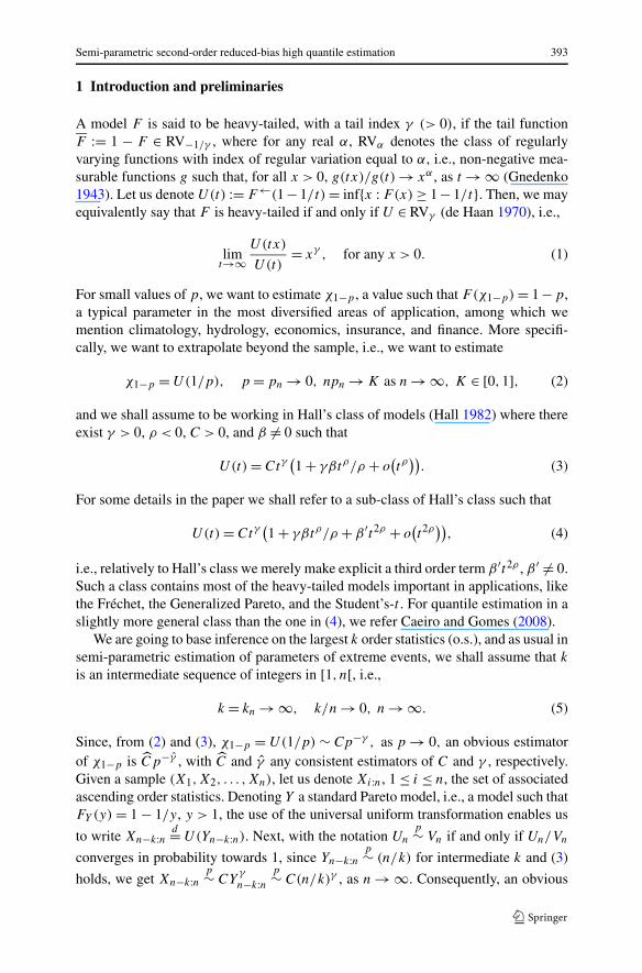
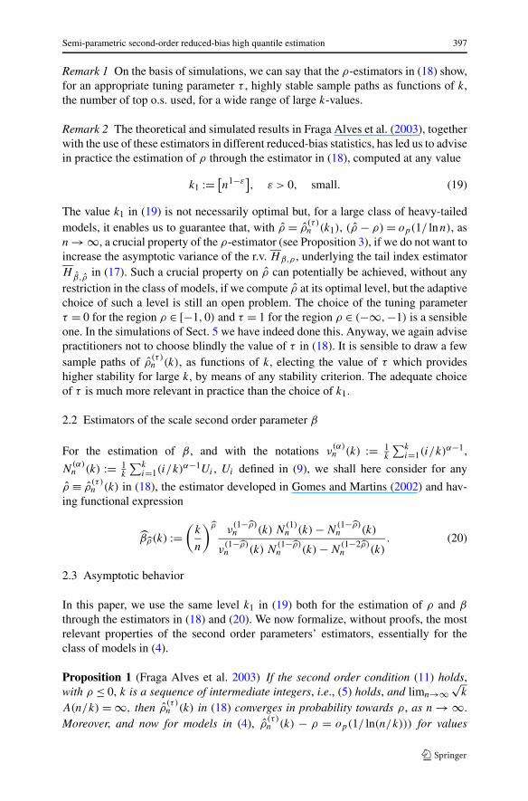
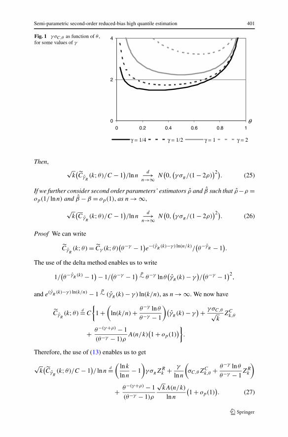
In Fig. 1, we picture γ σC,θ as a function of θ , for a few values of γ .The value of θ minimizing this standard deviation depends on γ , but the value

θ = 1/2, the one used later on in the simulations, seems to be a good choice amongθ ∈ (0,1), in the sense that the minimal variance is not a long way from the varianceat θ = 1/2.

Theorem 2 Under the conditions in Theorem 1, assume that√

k A(n/k) → λ andγ

R≡ γ

R(k) is a second order reduced-bias tail index estimator, such that (13) holds.

Semi-parametric second-order reduced-bias high quantile estimation 401

Fig. 1 γ σC,θ as function of θ ,for some values of γ

Then,√

k(Cγ

R(k; θ)/C − 1

)/lnn

d−→n→∞ N

(0,

(γ σ

R/(1 − 2ρ)

)2). (25)

If we further consider second order parameters’ estimators ρ and β such that ρ−ρ =op(1/ lnn) and β − β = op(1), as n → ∞,

√k(Cγ

R(k; θ)/C − 1

)/lnn

d−→n→∞ N

(0,

(γ σ

R/(1 − 2ρ)

)2). (26)

Proof We can write

CγR(k; θ) = Cγ (k; θ)

(θ−γ − 1

)e−(γ

R(k)−γ ) ln(n/k)/

(θ−γ

R − 1).

The use of the delta method enables us to write

1/(θ−γ

R(k) − 1

) − 1/(θ−γ − 1

) p∼ θ−γ ln θ(γ

R(k) − γ

)/(θ−γ − 1

)2,

and e(γR

(k)−γ ) ln(k/n) − 1p∼ (γ

R(k) − γ ) ln(k/n), as n → ∞. We now have

CγR(k; θ)

d= C

{1 +

(ln(k/n) + θ−γ ln θ

θ−γ − 1

)(γ

R(k) − γ

) + γ σC,θ√k

ZCk,θ

+ θ−(γ+ρ) − 1

(θ−γ − 1)ρA(n/k)

(1 + op(1)

)}.

Therefore, the use of (13) enables us to get

√k(Cγ

R(k; θ)/C − 1

)/ lnn

d=(

ln k

lnn− 1

)γ σ

RZR

k + γ

lnn

(σC,θZ

Ck,θ + θ−γ ln θ

θ−γ − 1ZR

k

)

+ θ−(γ+ρ) − 1

(θ−γ − 1)ρ

√kA(n/k)

lnn

(1 + op(1)

). (27)

402 F. Caeiro, M.I. Gomes

If we consider k-values, such that√

k A(n/k) → λ, non-null and finite, we haveln k/ lnn → −2ρ/(1 − 2ρ), as n → ∞, and the result in (25) follows.

Now, since CγR(k; θ) = Cγ

R(k; θ) × (1 − (θ

−(γR

+ρ)−1)

θ−γ

R −1

γR

β(n/k)ρ

ρ), the use of the

delta method enables us to write,

(θ−(γ

R+ρ) − 1

θ−γR − 1

)γ

Rβ

ρ

(n

k

)ρ

= θ−(γ+ρ) − 1

θ−γ − 1

A(n/k)

ρ

×[

1 +(

1 − γ θ−γ (θ−ρ − 1)

(θ−γ − 1)(θ−(γ+ρ) − 1)

)γ

R− γ

γ

+ β − β

β+ (ρ − ρ) ln(n/k)

].

As γR

− γ = op(1), (ρ − ρ) ln(n/k) = op(1) and β − β = op(1), we have

(θ−γ

R+ρ − 1

θ−γR − 1

)γ

Rβ

ρ

(n

k

)ρ

= θ−(γ+ρ) − 1

θ−γ − 1

A(n/k)

ρ

(1 + op(1)

),

and

CγR(k; θ)

C

d= 1 +(

ln(k/n) + θ−γ ln θ

θ−γ − 1

)(γ

R(k) − γ

) + γ σC,θ√k

ZCk,θ + op

(A(n/k)

).

(28)

Therefore, with the notation WCk,θ := σC,θZ

Ck,θ + θ−γ ln θ

θ−γ −1 ZRk , we can write

√k(Cγ

R(k)/C − 1

)/lnn

d=(

lnk

lnn− 1

)γ σ

RZR

k + γ WCk,θ

lnn+ op

(√kA(n/k)

lnn

),

and the asymptotic result in (26) follows as well. �

Remark 5 Although both CγR(k; θ) and Cγ

R(k; θ) have the same limit distribution,

that result is achieved very slowly. In (27), the term θ−(γ+ρ)−1(θ−γ −1)ρ

√kA(n/k)

lnn(1 + op(1))

may change the bias of CγR

. Also, the term γWCk,θ / lnn may increase the variance of

any of the estimators.

4 The asymptotic behavior of reduced-bias quantile estimators

Details on semi-parametric estimation of extremely high quantiles for a general ex-treme value index γ ∈ R may be found in de Haan and Rootzén (1993) and morerecently in Ferreira et al. (2003). Matthys and Beirlant (2003), Gomes and Figueiredo(2006), Matthys et al. (2004), Gomes and Pestana (2007), and Beirlant et al. (2006)deal with heavy tails and reduced-bias quantile estimation.

Semi-parametric second-order reduced-bias high quantile estimation 403

Since we will work only with the asymptotic unbiased extreme value estimatorγ

R≡ H in (17), we shall next consider and study the high quantile estimator,

Q(p)

H(k; θ) := Xn−[θk]:n − Xn−k:n

θ−H(k) − 1

(k

np

)H(k)

× (1 − Bθ

(H(k), ρ, β

)). (29)

We may state the following results:

Theorem 3 Under the second order framework in (11) with A(t) = γβ tρ , for inter-mediate k, i.e., k such that (5) holds, whenever ln(np)/

√k → 0, and

√k A(n/k) →

λ, as n → ∞,

√k

ln( knp

)

(Q

(p)H (k)/χ1−p − 1

) d−→n→∞ Normal

(λ/(1 − ρ), γ 2). (30)

Moreover, for ρ and β such that β − β = op(1) and ρ − ρ = op(1/ lnn), as n → ∞,

√k

ln( knp

)

(Q

(p)

H(k; θ)/χ1−p − 1

) d−→n→∞ Normal

(0, γ 2). (31)

Proof Since χ1−p = U(1/p), and with γ = γ (k) any tail index estimator, one canwrite

Q(p)

γ(k) − χ1−p = Xn−k:n

((k/np)γ − U(1/p)/Xn−k:n

).

Using the second order condition (11) and the result in Proposition 4,

U(1/p)

Xn−k:n= U(n

k× k

np)

U(nk)

× U(nk)

Xn−k:n

d=(

k

np

)γ (1 + (

knp

)ρ−1

ρA(n/k)

(1 + o(1)

))

× (1 − γ Bk/

√k + op

(A(n/k)

)).

As ((k/(np))ρ − 1)/ρ → −1/ρ, we have

U(1/p)/Xn−k:nd=

(k

np

)γ (1 − γ Bk/

√k − A(n/k)/ρ + op

(A(n/k)

)).

The delta method enables us to write cγ d= cγ (1 + ln c(γ − γ )(1 + op(1))), for anyc > 0. Therefore, also using the result from Corollary 1, we get

Q(p)

γ(k) − χ1−p

d= C

(1

p

)γ [ln

(k

np

)(γ (k) − γ

) + γ√kBk + A(n/k)

ρ

(1 + o(1)

)],

(32)

404 F. Caeiro, M.I. Gomes

that is, since χ1−p ∼ Cp−γ ,

√k

ln( knp

)

(Q

(p)

γ(k)/χ1−p − 1

) d= √k(γ (k) − γ

) + γBk

ln( knp

)+

√kA(n/k)

ρ ln( knp

)

(1 + o(1)

).

Let us now replace the arbitrary tail index estimator γ by the Hill estimator H in (8).Since we consider

√k A(n/k) → λ, finite, as n → ∞, then ln( k

np) → ∞, and the

asymptotic result in (30) follows from (12).

Notice next that we can write Q(p)

H(k; θ) = CH (k; θ) p−H . Using χ1−p ∼ Cp−γ

and the same type of results used before for Q(p)

γ(k), as well as (28), one can write,

Q(p)

H(k; θ)

χ1−p

d= 1 +(

ln

(k

np

)+ θ−γ ln θ

θ−γ − 1

)(H(k) − γ

) + γ σC,θ√k

ZCk,θ + op

(A(n/k)

).

Therefore, since H(k) − γd= γ Zk/

√k + op(A(n/k)), and with the same notation

as before, WCk,θ := σC,θZ

Ck,θ + θ−γ ln θ

θ−γ −1 ZRk , we get

√k

ln( knp

)

(Q

(p)

H(k; θ)/χ1−p − 1

) d= γZk + γ WCk,θ

ln( knp

)+ op

(√kA(n/k)/ln

(k

np

)),

and (31) follows. �

Remark 6 Notice that, in (31), we have a mean value equal to 0, even if√

kA(n/k) →λ �= 0, as n → ∞.

Remark 7 Since ln( knp

) goes to infinity very slowly, we can state a better distribu-tional representation, for moderate k and n (pre-asymptotic case):

√k

ln( knp

)

(Q

(p)H (k)

χ1−p

− 1

)d≈ Normal

(λ

1 − ρ

(1 + 1 − ρ

ρ ln( knp

)

), γ 2

(1 + 1

ln2( knp

)

)),

√k

ln( knp

)

(Q

(p)

H(k; θ)

χ1−p

− 1

)d≈ Normal

(0, γ 2

({1 − s1(γ ; θ)

ln( knp

)

}2

+ 1 + s2(γ ; θ)

ln2( knp

)

)),

with s1(γ ; θ) = −θ−γ ln θ/(θ−γ − 1) and s2(γ ; θ) = (θ−γ /(θ−γ − 1))2. Notice that

s1(γ ; θ) → ∞ and s2(γ ; θ) → ∞ as γ → 0. The notation Xn

d≈ Yn means that Yn,a sequence of r.v.’s converging weakly towards Y , as n → ∞, gives a better approxi-mation to Xn than the asymptotic limit Y .

5 Finite sample behavior—a simulation study

We compare the finite sample behavior of the proposed high quantile estimator

Q(p)

H(k; θ) in (29), θ = 1/2, denoted Q

(p)

H(k) for the sake of simplicity, with the one

Semi-parametric second-order reduced-bias high quantile estimation 405

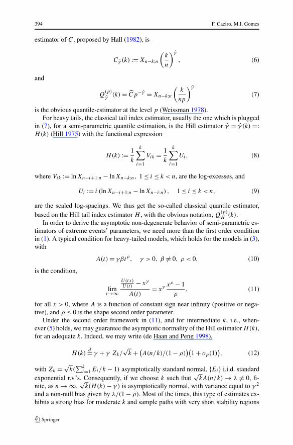
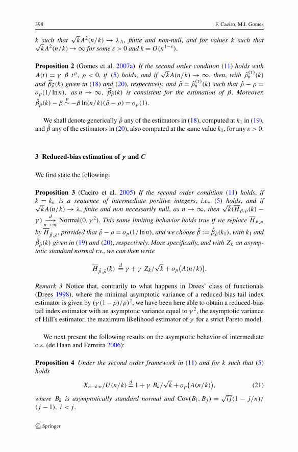
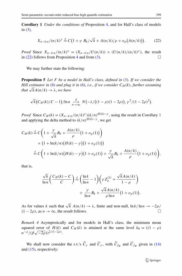
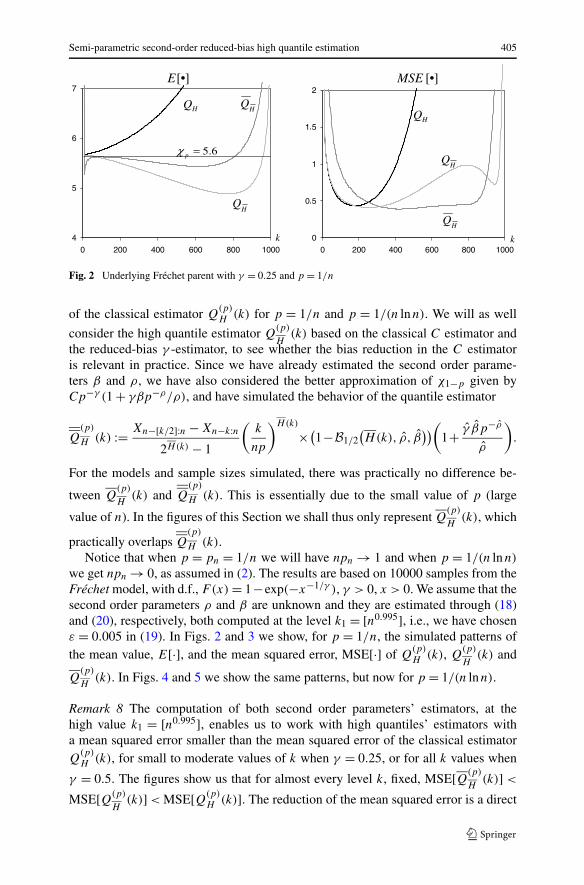
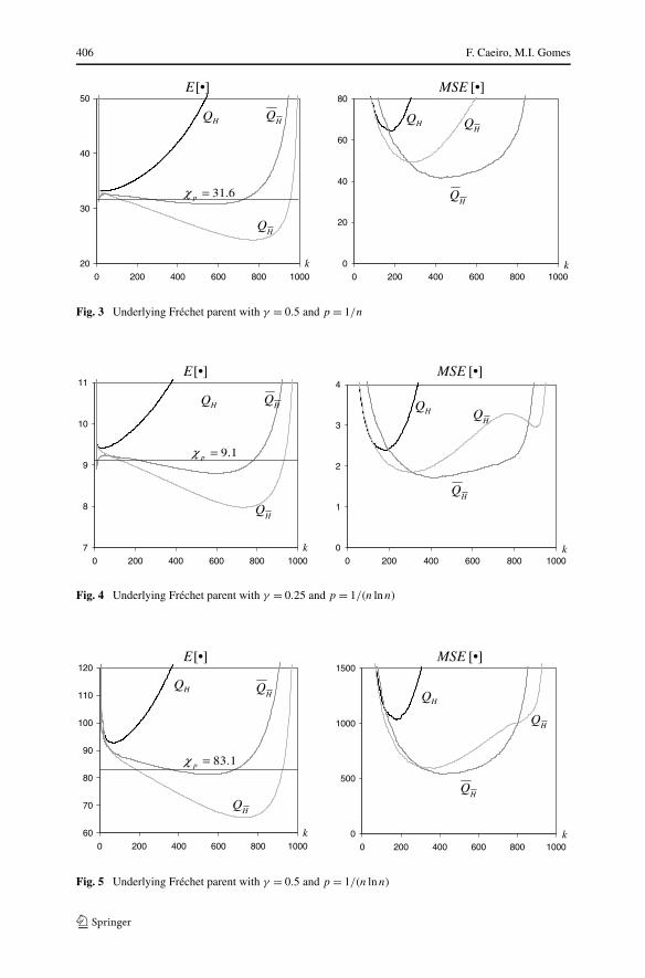
Fig. 2 Underlying Fréchet parent with γ = 0.25 and p = 1/n

of the classical estimator Q(p)H (k) for p = 1/n and p = 1/(n lnn). We will as well

consider the high quantile estimator Q(p)

H(k) based on the classical C estimator and

the reduced-bias γ -estimator, to see whether the bias reduction in the C estimatoris relevant in practice. Since we have already estimated the second order parame-ters β and ρ, we have also considered the better approximation of χ1−p given byCp−γ (1 + γβp−ρ/ρ), and have simulated the behavior of the quantile estimator

Q(p)

H (k) := Xn−[k/2]:n − Xn−k:n2H(k) − 1

(k

np

)H(k)

×(1− B1/2

(H(k), ρ, β

))(1+ γ βp−ρ

ρ

).

For the models and sample sizes simulated, there was practically no difference be-

tween Q(p)

H(k) and Q

(p)

H (k). This is essentially due to the small value of p (large

value of n). In the figures of this Section we shall thus only represent Q(p)

H(k), which

practically overlaps Q(p)

H (k).Notice that when p = pn = 1/n we will have npn → 1 and when p = 1/(n lnn)

we get npn → 0, as assumed in (2). The results are based on 10000 samples from theFréchet model, with d.f., F(x) = 1−exp(−x−1/γ ), γ > 0, x > 0. We assume that thesecond order parameters ρ and β are unknown and they are estimated through (18)and (20), respectively, both computed at the level k1 = [n0.995], i.e., we have chosenε = 0.005 in (19). In Figs. 2 and 3 we show, for p = 1/n, the simulated patterns ofthe mean value, E[·], and the mean squared error, MSE[·] of Q

(p)H (k), Q

(p)

H(k) and

Q(p)

H(k). In Figs. 4 and 5 we show the same patterns, but now for p = 1/(n lnn).

Remark 8 The computation of both second order parameters’ estimators, at thehigh value k1 = [n0.995], enables us to work with high quantiles’ estimators witha mean squared error smaller than the mean squared error of the classical estimatorQ

(p)H (k), for small to moderate values of k when γ = 0.25, or for all k values when

γ = 0.5. The figures show us that for almost every level k, fixed, MSE[Q(p)

H(k)] <

MSE[Q(p)

H(k)] < MSE[Q(p)

H (k)]. The reduction of the mean squared error is a direct

406 F. Caeiro, M.I. Gomes

Fig. 3 Underlying Fréchet parent with γ = 0.5 and p = 1/n

Fig. 4 Underlying Fréchet parent with γ = 0.25 and p = 1/(n lnn)

Fig. 5 Underlying Fréchet parent with γ = 0.5 and p = 1/(n lnn)

Semi-parametric second-order reduced-bias high quantile estimation 407

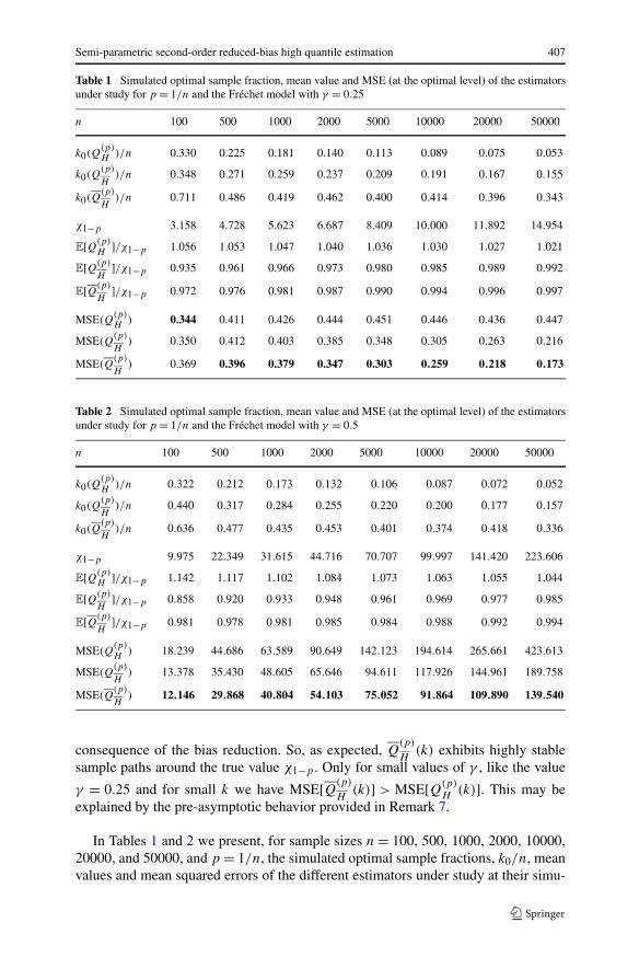
Table 1 Simulated optimal sample fraction, mean value and MSE (at the optimal level) of the estimatorsunder study for p = 1/n and the Fréchet model with γ = 0.25

n 100 500 1000 2000 5000 10000 20000 50000

k0(Q(p)H

)/n 0.330 0.225 0.181 0.140 0.113 0.089 0.075 0.053

k0(Q(p)

H)/n 0.348 0.271 0.259 0.237 0.209 0.191 0.167 0.155

k0(Q(p)

H)/n 0.711 0.486 0.419 0.462 0.400 0.414 0.396 0.343

χ1−p 3.158 4.728 5.623 6.687 8.409 10.000 11.892 14.954

E[Q(p)H

]/χ1−p 1.056 1.053 1.047 1.040 1.036 1.030 1.027 1.021

E[Q(p)

H]/χ1−p 0.935 0.961 0.966 0.973 0.980 0.985 0.989 0.992

E[Q(p)

H]/χ1−p 0.972 0.976 0.981 0.987 0.990 0.994 0.996 0.997

MSE(Q(p)H

) 0.344 0.411 0.426 0.444 0.451 0.446 0.436 0.447

MSE(Q(p)

H) 0.350 0.412 0.403 0.385 0.348 0.305 0.263 0.216

MSE(Q(p)

H) 0.369 0.396 0.379 0.347 0.303 0.259 0.218 0.173

Table 2 Simulated optimal sample fraction, mean value and MSE (at the optimal level) of the estimatorsunder study for p = 1/n and the Fréchet model with γ = 0.5

n 100 500 1000 2000 5000 10000 20000 50000

k0(Q(p)H

)/n 0.322 0.212 0.173 0.132 0.106 0.087 0.072 0.052

k0(Q(p)

H)/n 0.440 0.317 0.284 0.255 0.220 0.200 0.177 0.157

k0(Q(p)

H)/n 0.636 0.477 0.435 0.453 0.401 0.374 0.418 0.336

χ1−p 9.975 22.349 31.615 44.716 70.707 99.997 141.420 223.606

E[Q(p)H

]/χ1−p 1.142 1.117 1.102 1.084 1.073 1.063 1.055 1.044

E[Q(p)

H]/χ1−p 0.858 0.920 0.933 0.948 0.961 0.969 0.977 0.985

E[Q(p)

H]/χ1−p 0.981 0.978 0.981 0.985 0.984 0.988 0.992 0.994

MSE(Q(p)H

) 18.239 44.686 63.589 90.649 142.123 194.614 265.661 423.613

MSE(Q(p)

H) 13.378 35.430 48.605 65.646 94.611 117.926 144.961 189.758

MSE(Q(p)

H) 12.146 29.868 40.804 54.103 75.052 91.864 109.890 139.540

consequence of the bias reduction. So, as expected, Q(p)

H(k) exhibits highly stable

sample paths around the true value χ1−p . Only for small values of γ , like the value

γ = 0.25 and for small k we have MSE[Q(p)

H(k)] > MSE[Q(p)

H (k)]. This may beexplained by the pre-asymptotic behavior provided in Remark 7.

In Tables 1 and 2 we present, for sample sizes n = 100, 500, 1000, 2000, 10000,20000, and 50000, and p = 1/n, the simulated optimal sample fractions, k0/n, meanvalues and mean squared errors of the different estimators under study at their simu-

408 F. Caeiro, M.I. Gomes

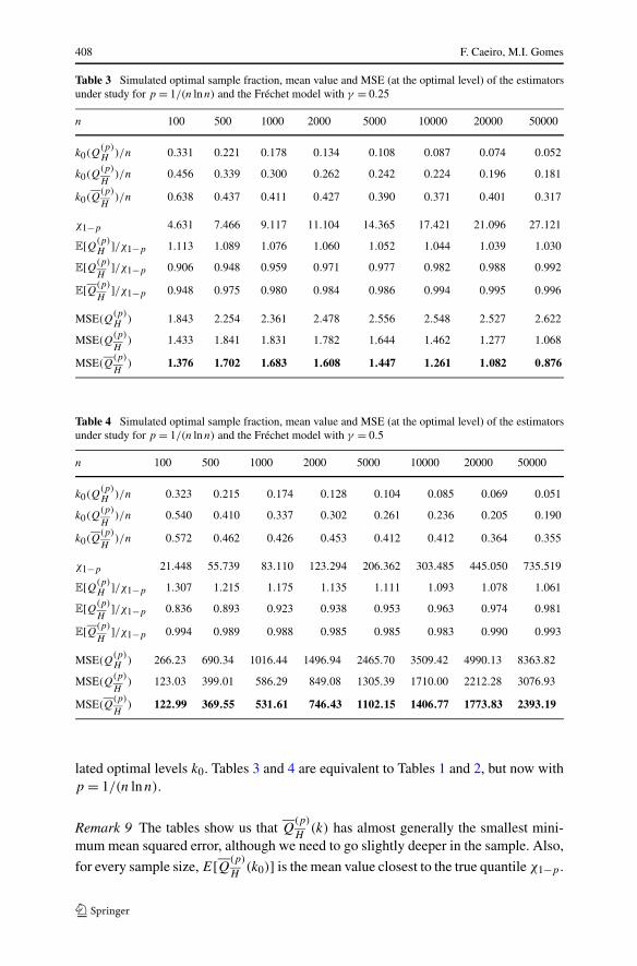
Table 3 Simulated optimal sample fraction, mean value and MSE (at the optimal level) of the estimatorsunder study for p = 1/(n lnn) and the Fréchet model with γ = 0.25

n 100 500 1000 2000 5000 10000 20000 50000

k0(Q(p)H

)/n 0.331 0.221 0.178 0.134 0.108 0.087 0.074 0.052

k0(Q(p)

H)/n 0.456 0.339 0.300 0.262 0.242 0.224 0.196 0.181

k0(Q(p)

H)/n 0.638 0.437 0.411 0.427 0.390 0.371 0.401 0.317

χ1−p 4.631 7.466 9.117 11.104 14.365 17.421 21.096 27.121

E[Q(p)H

]/χ1−p 1.113 1.089 1.076 1.060 1.052 1.044 1.039 1.030

E[Q(p)

H]/χ1−p 0.906 0.948 0.959 0.971 0.977 0.982 0.988 0.992

E[Q(p)

H]/χ1−p 0.948 0.975 0.980 0.984 0.986 0.994 0.995 0.996

MSE(Q(p)H

) 1.843 2.254 2.361 2.478 2.556 2.548 2.527 2.622

MSE(Q(p)

H) 1.433 1.841 1.831 1.782 1.644 1.462 1.277 1.068

MSE(Q(p)

H) 1.376 1.702 1.683 1.608 1.447 1.261 1.082 0.876

Table 4 Simulated optimal sample fraction, mean value and MSE (at the optimal level) of the estimatorsunder study for p = 1/(n lnn) and the Fréchet model with γ = 0.5

n 100 500 1000 2000 5000 10000 20000 50000

k0(Q(p)H

)/n 0.323 0.215 0.174 0.128 0.104 0.085 0.069 0.051

k0(Q(p)

H)/n 0.540 0.410 0.337 0.302 0.261 0.236 0.205 0.190

k0(Q(p)

H)/n 0.572 0.462 0.426 0.453 0.412 0.412 0.364 0.355

χ1−p 21.448 55.739 83.110 123.294 206.362 303.485 445.050 735.519

E[Q(p)H

]/χ1−p 1.307 1.215 1.175 1.135 1.111 1.093 1.078 1.061

E[Q(p)

H]/χ1−p 0.836 0.893 0.923 0.938 0.953 0.963 0.974 0.981

E[Q(p)

H]/χ1−p 0.994 0.989 0.988 0.985 0.985 0.983 0.990 0.993

MSE(Q(p)H

) 266.23 690.34 1016.44 1496.94 2465.70 3509.42 4990.13 8363.82

MSE(Q(p)

H) 123.03 399.01 586.29 849.08 1305.39 1710.00 2212.28 3076.93

MSE(Q(p)

H) 122.99 369.55 531.61 746.43 1102.15 1406.77 1773.83 2393.19

lated optimal levels k0. Tables 3 and 4 are equivalent to Tables 1 and 2, but now withp = 1/(n lnn).

Remark 9 The tables show us that Q(p)

H(k) has almost generally the smallest mini-

mum mean squared error, although we need to go slightly deeper in the sample. Also,

for every sample size, E[Q(p)

H(k0)] is the mean value closest to the true quantile χ1−p .

Semi-parametric second-order reduced-bias high quantile estimation 409

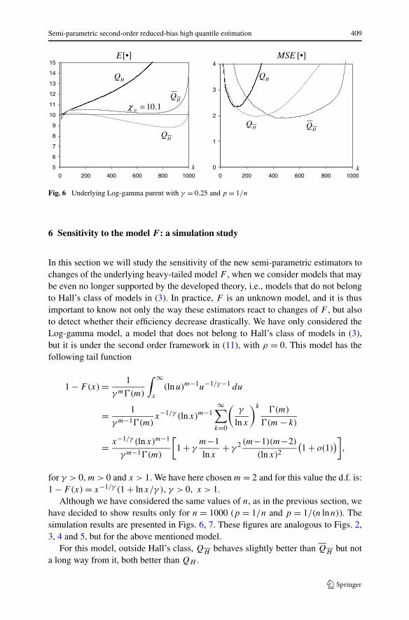
Fig. 6 Underlying Log-gamma parent with γ = 0.25 and p = 1/n

6 Sensitivity to the model F : a simulation study

In this section we will study the sensitivity of the new semi-parametric estimators tochanges of the underlying heavy-tailed model F , when we consider models that maybe even no longer supported by the developed theory, i.e., models that do not belongto Hall’s class of models in (3). In practice, F is an unknown model, and it is thusimportant to know not only the way these estimators react to changes of F , but alsoto detect whether their efficiency decrease drastically. We have only considered theLog-gamma model, a model that does not belong to Hall’s class of models in (3),but it is under the second order framework in (11), with ρ = 0. This model has thefollowing tail function

1 − F(x) = 1

γ m (m)

∫ ∞

x

(lnu)m−1u−1/γ−1 du

= 1

γ m−1 (m)x−1/γ (lnx)m−1

∞∑

k=0

(γ

lnx

)k (m)

(m − k)

= x−1/γ (lnx)m−1

γ m−1 (m)

[1 + γ

m−1

lnx+ γ 2 (m−1)(m−2)

(lnx)2

(1 + o(1)

)],

for γ > 0, m > 0 and x > 1. We have here chosen m = 2 and for this value the d.f. is:1 − F(x) = x−1/γ (1 + lnx/γ ), γ > 0, x > 1.

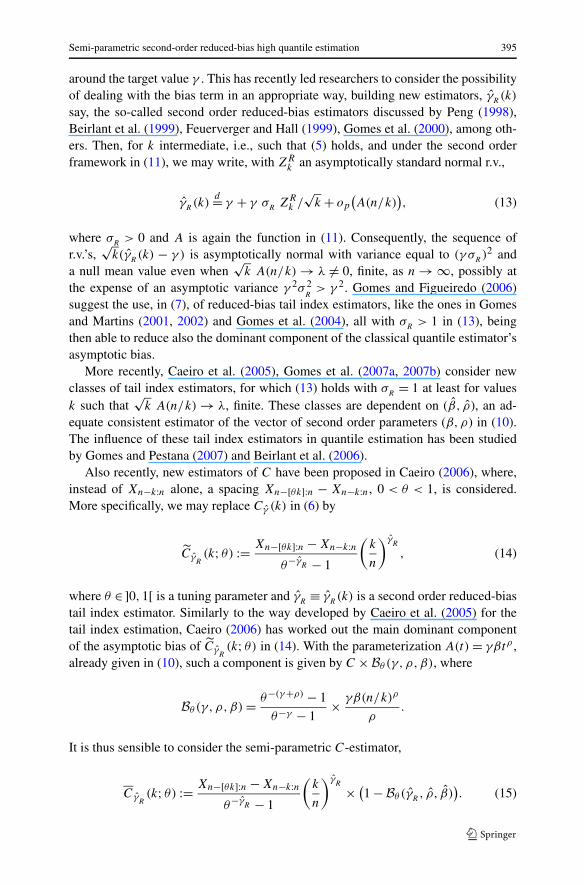
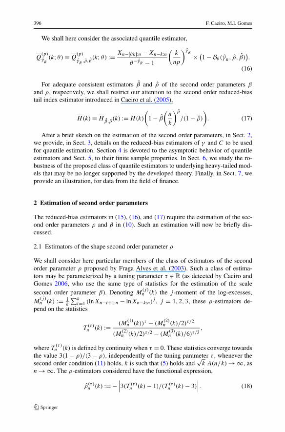
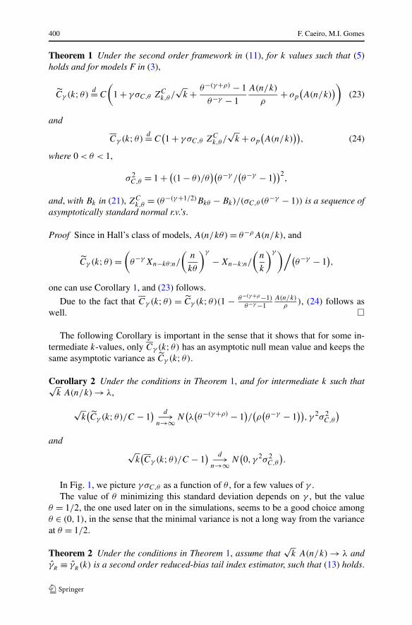
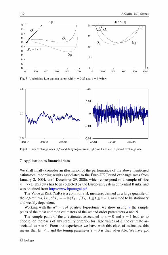
Although we have considered the same values of n, as in the previous section, wehave decided to show results only for n = 1000 (p = 1/n and p = 1/(n lnn)). Thesimulation results are presented in Figs. 6, 7. These figures are analogous to Figs. 2,3, 4 and 5, but for the above mentioned model.

For this model, outside Hall’s class, QH behaves slightly better than QH but nota long way from it, both better than QH .

410 F. Caeiro, M.I. Gomes

Fig. 7 Underlying Log-gamma parent with γ = 0.25 and p = 1/n lnn

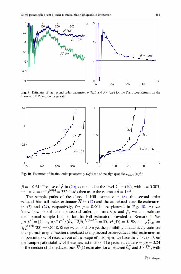
Fig. 8 Daily exchange rates (left) and daily log-returns (right) on Euro vs UK pound exchange rate

7 Application to financial data

We shall finally consider an illustration of the performance of the above mentionedestimators, reporting results associated to the Euro-UK Pound exchange rates fromJanuary 2, 2004, until December 29, 2006, which correspond to a sample of sizen = 771. This data has been collected by the European System of Central Banks, andwas obtained from http://www.bportugal.pt/.

The Value at Risk (VaR) is a common risk measure, defined as a large quantile ofthe log-returns, i.e., of Lt = − ln(Xt+1/Xt ), 1 ≤ t ≤ n − 1, assumed to be stationaryand weakly dependent.

Working with the n+ = 384 positive log-returns, we show in Fig. 9 the samplepaths of the most common estimators of the second order parameters ρ and β .

The sample paths of the ρ-estimates associated to τ = 0 and τ = 1 lead us tochoose, on the basis of any stability criterion for large values of k, the estimate as-sociated to τ = 0. From the experience we have with this class of estimates, thismeans that |ρ| ≤ 1 and the tuning parameter τ = 0 is then advisable. We have got

Semi-parametric second-order reduced-bias high quantile estimation 411

Fig. 9 Estimates of the second-order parameter ρ (left) and β (right) for the Daily Log-Returns on theEuro vs UK Pound exchange rate

Fig. 10 Estimates of the first-order parameter γ (left) and of the high quantile χ0.001 (right)

ρ = −0.61. The use of β in (20), computed at the level k1 in (19), with ε = 0.005,i.e., at k1 = (n+)0.995 = 372, leads then us to the estimate β = 1.06.

The sample paths of the classical Hill estimator in (8), the second orderreduced-bias tail index estimator H in (17) and the associated quantile-estimatorsin (7) and (29), respectively, for p = 0.001, are pictured in Fig. 10. As weknow how to estimate the second order parameters ρ and β , we can estimatethe optimal sample fraction for the Hill estimator, provided in Remark 4. Weget kH

0 = [(1 − ρ)(n+)−ρ/(β√−2ρ)]2/(1−2ρ) = 35, H(35) = 0.198, and χH

0.001 :=Q

(0.001)H (35) = 0.0118. Since we do not have yet the possibility of adaptively estimate

the optimal sample fraction associated to any second order reduced-bias estimator, animportant topic of research out of the scope of this paper, we base the choice of k onthe sample path stability of these new estimators. The pictured value γ = γR = 0.24is the median of the reduced-bias H(k) estimates for k between kH

0 and 3 × kH0 , with

412 F. Caeiro, M.I. Gomes

the subscript R standing for reduced-bias. A similar technique led us to the quantileestimate χR

0.001 = 0.0196, as pictured in Fig. 10(right). Note that p = 0.001 < 1/n,i.e., we are extrapolating beyond the sample.

To study the out-of-sample performance of the high quantile estimator, we haveadded more data to the sample. Since we are estimating a very high quantile, wehave considered all available data, from January 4, 1999, until December 31, 2007,which corresponds to a sample of size n′ = 2303. The non parametric 90% confi-dence interval (Conover 1998) for the desired quantile of probability 1 − p = 0.999is given by

(L2298:2303;L2303:2303) = (0.0136;0.0201).

Notice that the previous reduced-bias high quantile estimate, χR0.001 = 0.0196, be-

longs to this confidence interval, whereas χH0.001 = 0.0118 does not. Moreover, we

get for p the estimate pR = 0.0004 and an associated 90% confidence interval givenby (0,0.0011), also covering the value p = 0.001, whereas pH = 0.0052 is quitehigh, and the associated 90% confidence interval, given by (0.0027,0.0077), doesnot cover p = 0.001. This is thus a point in favor of the reduced-bias estimators con-sidered in this paper.

References

Beirlant J, Dierckx G, Goegebeur Y, Matthys G (1999) Tail index estimation and an exponential regressionmodel. Extremes 2:177–200

Beirlant J, Figueiredo F, Gomes MI, Vandewalle B (2006) Improved reduced bias tail index and quantileestimators. J Stat Plan Inference. doi:10.1016/j.jspi.2007.07.015

Caeiro F (2006) Estimação de parâmetros de acontecimentos raros. PhD thesis, FCUL, Universidade deLisboa

Caeiro F, Gomes MI (2006) A new class of estimators of a “scale” second order parameter. Extremes9:193–211

Caeiro F, Gomes MI (2008) Minimum-variance reduced-bias tail index and high quantile estimation. Rev-stat 6(1):1–20

Caeiro F, Gomes MI, Pestana D (2005) Direct reduction of bias of the classical Hill estimator. Revstat3(2):113–136

Conover WJ (1998) Practical nonparametric statistics, 3rd edn. Wiley, New Yorkde Haan L (1970) On regular variation and its application to the weak convergence of sample extremes.

Mathematical Centre Tract 32, Amsterdamde Haan L, Ferreira A (2006) Extreme value theory: an introduction. Springer, New Yorkde Haan L, Peng L (1998) Comparison of tail index estimators. Stat Neerl 52:60–70de Haan L, Rootzén H (1993) On the estimation of high quantiles. J Stat Plan Inference 35:1–13Drees H (1998) On smooth statistical tail functionals. Scand J Stat 25:187–210Ferreira A, de Haan L, and Peng L (2003) On optimising the estimation of high quantiles of a probability

distribution. Statistics 37(5):401–434Feuerverger A, Hall P (1999) Estimating a tail exponent by modelling departure from a Pareto distribution.

Ann Stat 27:760–781Fraga Alves MI, Gomes MI, de Haan L (2003) A new class of semi-parametric estimators of the second

order parameter. Port Math 60(1):193–213Gnedenko BV (1943) Sur la distribution limite du terme maximum d’une série aléatoire. Ann Math

44:423–453Gomes MI, Figueiredo F (2006) Bias reduction in risk modelling: semi-parametric quantile estimation.

Test 15(2):375–396Gomes MI, Martins MJ (2001) Generalizations of the Hill estimator—asymptotic versus finite sample

behavior. J Stat Plan Inference 93:161–180

Semi-parametric second-order reduced-bias high quantile estimation 413

Gomes MI, Martins MJ (2002) “Asymptotically unbiased” estimators of the tail index based on externalestimation of the second order parameter. Extremes 5(1):5–31

Gomes MI, Pestana D (2007) A sturdy reduced bias extreme quantile (VaR) estimator. J Am Stat Assoc102(477):280–292

Gomes MI, Martins MJ, Neves M (2000) Alternatives to a semi-parametric estimator of parameters of rareevents—the Jackknife methodology. Extremes 3(3):207–229

Gomes MI, Caeiro F, Figueiredo F (2004) Bias reduction of a tail index estimator through an externalestimation of the second order parameter. Statistics 38(6):497–510

Gomes MI, de Haan L, and Henriques Rodrigues L (2007a) Tail index estimation for heavy-tailed models:accommodation of bias in the weighted log-excesses. J R Stat Soc B 69(5):1–22

Gomes MI, Martins MJ, Neves M (2007b) Improving second order reduced bias extreme value indexestimation. Revstat 5(2):177–207

Hall P (1982) On some simple estimates of an exponent of regular variation. J R Stat Soc 44(1):37–42Hill BM (1975) A simple general approach to inference about the tail of a distribution. Ann Stat 3(5):1163–

1174Matthys G, Beirlant J (2003) Estimating the extreme value index and high quantiles with exponential

regression models. Stat Sin 13:853–880Matthys G, Delafosse M, Guillou A, Beirlant J (2004) Estimating catastrophic quantile levels for heavy-

tailed distributions. Insur Math Econ 34:517–537Peng L (1998) Asymptotic unbiased estimator for the extreme-value index. Stat Probab Lett 38:107–115Weissman I (1978) Estimation of parameters of large quantiles based on the k largest observations. J Am

Stat Assoc 73:812–815