TI 2013-020/III Tinbergen Institute Discussion Paper

Return-Volatility Relationship: Insights from Linear and Non-Linear Quantile Regression

David E. Allena

Abhay K. Singha

Robert J. Powella

Michael McAleerb

James Taylorc Lyn Thomasd

aSchool of Accouting Finance & Economics, Edith Cowan University, Australia; b Econometric Institute, Erasmus School of Economics, Erasmus University Rotterdam, Tinbergen Institute, The Netherlands, Complutense University of Madrid, Spain, and Institute of Economic Research, Kyoto University, Japan; c Said Business School, University of Oxford, Oxford; dSouthampton Management School, University of Southampton, Southampton.

Tinbergen Institute is the graduate school and research institute in economics of Erasmus University Rotterdam, the University of Amsterdam and VU University Amsterdam. More TI discussion papers can be downloaded at http://www.tinbergen.nl Tinbergen Institute has two locations: Tinbergen Institute Amsterdam Gustav Mahlerplein 117 1082 MS Amsterdam The Netherlands Tel.: +31(0)20 525 1600 Tinbergen Institute Rotterdam Burg. Oudlaan 50 3062 PA Rotterdam The Netherlands Tel.: +31(0)10 408 8900 Fax: +31(0)10 408 9031

Duisenberg school of finance is a collaboration of the Dutch financial sector and universities, with the ambition to support innovative research and offer top quality academic education in core areas of finance.

DSF research papers can be downloaded at: http://www.dsf.nl/ Duisenberg school of finance Gustav Mahlerplein 117 1082 MS Amsterdam The Netherlands Tel.: +31(0)20 525 8579

Return-Volatility Relationship: Insights fromLinear and Non-Linear Quantile Regression

David E Allena, Abhay K Singha, Robert J Powella, Michael McAleerb

James Taylorc & Lyn Thomasd

aSchool of Accouting Finance & Economics, Edith Cowan University, Australiab Econometric Institute, Erasmus School of Economics, Erasmus University Rotterdam, Tinbergen Institute, The

Netherlands, Department of Quantitative Economics, Complutense University of Madrid, Spain, and Institute of

Economic Research, Kyoto University, Japan

cSaid Business School, University of Oxford, OxforddSouthampton Management School, University of Southampton, Southampton

Abstract

The purpose of this paper is to examine the asymmetric relationship betweenprice and implied volatility and the associated extreme quantile dependence us-ing linear and non linear quantile regression approach. Our goal in this paper is todemonstrate that the relationship between the volatility and market return as quan-tified by Ordinary Least Square (OLS) regression is not uniform across the distribu-tion of the volatility-price return pairs using quantile regressions. We examine thebivariate relationship of six volatility-return pairs, viz. CBOE-VIX and S&P-500,FTSE-100 Volatility and FTSE-100, NASDAQ-100 Volatility (VXN) and NASDAQ,DAX Volatility (VDAX) and DAX-30, CAC Volatility (VCAC) and CAC-40 andSTOXX Volatility (VSTOXX) and STOXX. The assumption of a normal distribu-tion in the return series is not appropriate when the distribution is skewed and henceOLS does not capture the complete picture of the relationship. Quantile regressionon the other hand can be set up with various loss functions, both parametric andnon-parametric (linear case) and can be evaluated with skewed marginal based cop-ulas (for the non linear case). Which is helpful in evaluating the non-normal andnon-linear nature of the relationship between price and volatility. In the empiricalanalysis we compare the results from linear quantile regression (LQR) and copulabased non linear quantile regression known as copula quantile regression (CQR).The discussion of the properties of the volatility series and empirical findings inthis paper have significance for portfolio optimization, hedging strategies, tradingstrategies and risk management in general.

1

Keywords: Return-Volatility relationship, quantile regression, copula, copula quantileregression, volatility index, tail dependence.

2

1 Introduction

Quantifiction of relationship between the change in stock index return and changes in thevolatility index serves as the basis for hedging. This relationship is mostly quantified asbeing asymmetric (Badshah, 2012; Dennis, Mayhew & Stivers, 2006; Fleming, Ostdiek,& Whaley, 1995; Giot, 2005; Hibbert, Daigler, & Dupoyet, 2008; Low, 2004; Whaley,2000; Wu, 2001). Asymmetric relationship means that the negative change in the stockmarket has higher impact on the volatility index than a positive change or vice versa. Theasymmetric volatility-return relationship has been pointed out in two hypothesis i.e., theleverage hypothesis (Black, 1976; Christie, 1982) and the volatility feedback hypothesis(Campbell and Hentchel, 1992).

In a call/put option contract time to maturity and strike price form its basic charac-teristics, the other inputs viz., risk free rate and divident payout can be decided easily(Black and Scholes, 1973). When pricing an option the expected volatility over the lifeof the option becomes a critical input, it is also the only input which is not directlyobserved by market participants. In an actively traded market volatility can be calcu-lated by inverting the chosen option pricing formula for the observed market price of theoption. This volatility calculated by inverting the option pricing formula is known asimplied volatility. With increasing focus on risk modelling in modern finance modellingand predicting asset volatility along with its dependence with the underlying asset classhas become an important research topic.

The change in volatility leads to the movement in the stock market prices. For examplean expected rise in volatility will lead to a decline in stock market prices. The volatilityindices are used for option pricing and hedging calculations and the change in them getsreflected on the corresponding stock markets. Financial risk is mostly composed of rareor extreme events which results in high risk and lies in the tail of the return distribution.In option pricing rare or extreme events results in volatility skew patterns (Liu, Pan andWang, 2005).

3

Figure 1: Time Series Plot VIX and S&P 500

Ordinary least squares regression method is the most widely used method for quantify-ing a relationship between two class of assets or return distribution in finance literature.Figure-1, shows the logarithmic return series of VIX and S&P-500 stock indices fromyear 2008-2011. The time series plot shows that the VIX index change according to thechange in S&P-500. We employ two cases of quantile regression (linear and non-linear)to evaluate the asymmetric volatility-return relationship between change in the volatilityindex (VIX, VFTSE,VXN, VDAX, VSTOXX and VCAC) and corresponding stock indexreturn (S&P-500, FTSE-100, NASDAQ, DAX-30, STOXX and CAC-40). We focus onthe daily asymmetric return-volatility relation in this study.

Giot (2005), Hibbert et al. (2008) and Low (2004) use OLS in their study of asymmet-ric return-volatility relationship across implied volatility (IV) change distribution. OLSas it is evaluation is based on the deviations from the mean of the distribution under-estimates the extreme quantile relationships. Badshah (2012) extends the past studiesusing LQR to estimate the negative asymmetric return-volatility relationship betweenstock index return (S&P-500, NASDAQ, DAX-30,STOXX ) and changes in volatilityindex return (VIX, VXN, VDAX, VSTOXX) for lower and upper quantiles which givenegative and positive returns . In his study Badshah (2012) found that negative returnshas higher impacts than the positive returns using linear quantile regression framework.Kumar (2012), used LQR to examine the statistical properties of volatility index of Indiaand its relationship with Indian stock market.

4

Figure 2: Q-Q Plots

Figure-2, gives the quantile-quantile plots for our data, none of the data series shownormality in its distribution. When the data distribution is not normal, QR can providemore efficient estimates for return-volatility relationship (Badshah, 2012). QR can notonly be used linearly but can also be evaluated for non-linear relationships using Copulabased models. The only comprehensive study (Badshah, 2012) done using QR on return-volatility relationship till now focus on linear case of the relationship. We extend thisstudy by considering the non-linear nature of the relationship using copula based nonlinear quantile regression models, CQR.

The rest of the paper is designed as follows; in section-2 we give details about linearquantile regression LQR, followed by non-linear quantile regression using copula CQRin section-3. In Section-4 we describe our data together with our research design andmethodology. We discuss the results in section-5 and conclude in section-6.

5

2 Quantile Regression

Regression analysis is undoubtedly the most widely used technique in market risk mod-elling, from factor models to model returns to autocorrelated models to model volatilityin time series. All models are based on regression analysis with different approaches.

A simple linear regression model can be written as:

Y = α + βX + ε, (1)

which represents the dependent variable, Y as a linear function of one or more in-dependent variable, X, subject to a random ‘disturbance’ or ‘error’ term, ε which isassumed to be i.i.d and independent of X.

A bivariate normal distribution is assumed between a dependent and independentvariable in simple linear regression. It estimates the mean value of the dependent variablefor given levels of the independent variables. For this type of regression, where we wantto understand the central tendency in a dataset, OLS is an effective method. OLS losesits effectiveness when we try to go beyond the median value or towards the extremesof a data set (see; Allen, Singh and Powell, 2010; Allen, Gerrans, Singh and Powell,2009; Barnes and Hughes, 2002). Specifically in the case of an unknown or arbitraryjoint distribution (X, Y ), OLS does not provide all the necessary information required toquantify the conditional distribution of the dependent variable. As given in descriptivestatistics (section-4.1) the dataset used in this analysis is not normal and hence quantileregression can be a better choice.

Quantile Regression is modelled as an extension of classical OLS (Koenker and Bas-sett, 1978). In Quantile Regression the estimation of conditional mean as estimated byOLS is extended to similar estimation of an ensemble of models of various conditionalquantile functions for a data distribution. In this fashion Quantile Regression can betterquantify the conditional distribution of (Y |X). The central special case is the medianregression estimator that minimises a sum of absolute errors. The estimates of remainingconditional quantile functions are obtained by minimizing an asymmetrically weightedsum of absolute errors, where weights are the function of the quantile of interest. Thismakes Quantile Regression a robust technique even in presence of outliers. Taken to-gether the ensemble of estimated conditional quantile functions of (Y |X) offers a muchmore complete view of the effect of covariates on the location, scale and shape of thedistribution of the response variable.

For parameter estimation in Quantile Regression, quantiles as proposed by Koenkerand Bassett (1978) can be defined through an optimisation problem. To solve an OLSregression problem a sample mean is defined as the solution of the problem of minimisingthe sum of squared residuals, in the same way the median quantile (0.5%) in QuantileRegression is defined through the problem of minimising the sum of absolute residuals.

6

The symmetrical piecewise linear absolute value function assures the same number ofobservations above and below the median of the distribution.

The other quantile values can be obtained by minimizing a sum of asymmetricallyweighted absolute residuals, (giving different weights to positive and negative residuals).Solving

minξεR∑

ρτ (yi − ξ) (2)

Where ρτ (�) is the tilted absolute value function as shown in Figure 2.4, which gives theτth sample quantile with its solution. Taking the directional derivatives of the objectivefunction with respect to ξ (from left to right) shows that this problem yields the samplequantile as its solution.

Figure 3: Quantile Regression ρ Function

After defining the unconditional quantiles as an optimisation problem, it is easy todefine conditional quantiles similarly. Taking the least squares regression model as a baseto proceed, for a random sample, y1, y2, . . . , yn, we solve

minµεR

n∑i=1

(yi − µ)2 (3)

which gives the sample mean, an estimate of the unconditional population mean, EY.Replacing the scalar µ by a parametric function µ(x, β) and then solving

minµεRp

n∑i=1

(yi − µ(xi, β))2 (4)

gives an estimate of the conditional expectation function E(Y|x).Proceeding the same way for Quantile Regression, to obtain an estimate of the con-

7

ditional median function, the scalar ξ in the first equation is replaced by the parametricfunction ξ(xt, β) and τ is set to 1/2 . The estimates of the other conditional quantilefunctions are obtained by replacing absolute values by ρτ (�) and solving

minµεRp

∑ρτ (yi − ξ(xi, β)) (5)

The resulting minimization problem, when ξ(x, β) is formulated as a linear function ofparameters, and can be solved very efficiently by linear programming methods. Furtherinsight into this robust regression technique can be obtained from Koenkar and Bassett’sQuantile Regression monograph (2005) or a text book introduction to Quantile Regressionas can be found in Alexandar (2008).

Quantile regression has been frequently tested in research work over the past decadein various areas of econometric analysis, financial modelling and socio-economic research.The studies include Buchinsky and Leslie (1997) who analyse changing US wage struc-tures. Buchinsky and Hunt (1999) analyse the earning mobility and factors affectingthe transmission of earnings across generations. Eide and Showanter (1998) study theeffect of school quality on education. Financial research work using Quantile Regres-sion includes Engle and Manganelli (2004) and Morillo (2000) quantifying VaR usingQuantile Regression and studying option pricing using Monte Carlo simulations. Barnesand Hughes (2002) applied Quantile Regression to study CAPM in their work on crosssections of stock market returns. Chan and Lakonishok (1992) applied Quantile Regres-sion to robust measurement of size and book to market effects. Gowlland, Xiao andZeng (2009) investigate book to market effect beyond central tendency. Allen, Singh andPowell (2011), apply Quantile Regression to test the Fama-French factor model in theDJIA-30 stocks which focuses on the applicability of better estimates of factor based riskfactors across quantiles.

Other than Badshah (2012) and Kumar (2012) there is no prior work done on in-vestigating the return-volatility relationship between volatiltiy indices and correspondingmarket indices using quantile regression. We not only apply the LQR model to evaluatethe return-volatility relationship but we also test the non-linear case of CQR to examinethe relationship.

3 Non-Linear Quantile Regression (CQR)

Bouyé and Salmon (2009) extended Koenker and Basset’s (1978) idea of regression quan-tiles and introduced a general approach to non linear quantile regression modelling usingcopula functions. Copula functions are used to define the dependence structure betweenthe dependent and independent variables of interest. We first give a brief introductionto copula followed by the introduction to the concept of CQR.

8

3.1 Copula

Modelling dependency structure within assets is a key issue in risk measurement. Themost common measure for dependency, correlation, loses its effect when a dependencymeasure is required for distribution which deviates from the mean or are not normallydistributed. Examples of deviations from normality are the presence of kurtosis or fattails and skewness in univariate distributions. Deviation from normality also occursin multivariate distributions given by asymmetric dependence, which infers that assetsshow different level of correlation during different market conditions (Erb et al., 1994;Longin and Solnik, 2001; Ang and Chen, 2002 and Patton, 2004). Modelling dependencewith correlation is not inefficient when the distribution follow the strict assumptions ofnormality and constant dependence across the quantiles. But as now it is well known infinancial risk modelling, return distribution does not necessarily follow normality acrossquantiles, we need more sophisticated tools for modelling dependence than correlationand Copulas provide one such measure.

The statistical tool which is used to model the underlying dependence structure ofa multivariate distribution is the copula function. The capability of copula to modeland estimate multivariate distributions comes from Sklar’s Theorem, according to whicheach joint distribution can be decomposed into its marginal distributions and a copulaC responsible for the dependence structure. Here we define Copula with Sklar’s theoremalong with some important types of copula, adapted from Franke, Härdle and Hafner(2008).

A function C : [0, 1]d → [0, 1] is a d dimensional copula if it satisfies the followingconditions for every u = (u1, . . . , ud)

> ∈ [0, 1]d and j ∈ {1, . . . , d}

1. if uj = 0 then C(u1, . . . , ud) = 0

2. C(1, . . . , 1, uj, 1, . . . , 1) = uj

3. for every υ = (υ1, . . . , υd)> ∈ [0, 1]d, υj ≤ uj

VC(u, υ) ≥ 0

where VC(u, υ) is given by

2∑i1=1

. . .2∑

id=1

(−1)i1+...+idC(g1i1 , . . . , gdid)

Properties 1 and 3 state that copulae are grounded functions and that all d-dimensionalboxes with vertices in [0, 1]d have non-negative C-volume. Property second shows thatthe copulae have uniform marginal distributions.

9

Sklar’s Theorem

Consider a d-dimensional distribution function F with marginals F1 . . . , Fd. Then forevery x1, . . . , xd ∈ R, a copula, C can exist with

F (x1, . . . , xd) = C{F1(x1), . . . , Fd(xd)} (6)

C is unique if F1 . . . , Fd are continuous. If F1, . . . , Fd are distributions then the func-tion F is a joint distribution function with marginals F1, . . . , Fd.

For a joint distribution F with continuous marginals F1, . . . , Fd , for all u = (u1, . . . , ud)> ∈

[0, 1]d the unique copula C is given as

C(u1, . . . , ud) = F{F−11 (u1), . . . , F−1d (ud)} (7)

Copula can be divided into two broad types, Elliptical Copulae-Gaussian Copula andStudent’s t-copula and Archimedean Copulae-Gumbel copula and Clayton copula andFrank Copula .

Normal or Gaussian Copula

The copula derived from the n-dimensional multivariate and univariate standard normaldistribution functions, Φ and Φ, is called a normal or gaussian copula. The normal copulacan be defined as

C(u1, . . . , un; Σ) = Φ(Φ−1(u1), . . . ,Φ

−1(un))

(8)

where correlation matrix(Σ) is the parameter for normal copula and ui = Fi(xi) isthe marginal distribution function.

The normal copula density is given by

c(u1, . . . , un; Σ) = |Σ|−1/2 exp

(−1

2ξ′(Σ−1 − I)ξ

)(9)

where Σ is the correlation matrix, |Σ| is its determinant. ξ = (ξ1, . . . , ξn)′, where ξiis the ui quantile of the standard normal variable Xi.

Figure- 4 gives the density plot for a bivariate gaussian copula with a correlation of0.5. As shown in the figure, normal copula is a symmetric copula.

Student’s t-Copula

Similar to gaussian copula, t-copula models the dependence structure of multivariate t-distributions. The parameters for student’s t-copula are correlation matrix and degreesof freedom. Student’s t-copula show symmetrical dependence but are higher than those

10

Figure 4: Density of the Gaussian copula

in gaussian copula as shown in figure-5. Kindly refer Alexandar (2008) for the densityfunctions and quantile functions of student-t copula.

Figure 5: Density of t-copula

11

Archimedean Copulae

Archimedean copulae are family of copulae which are build on a generator function,with some restrictions. There can be various copulae in this family of copulae due tovarious generator functions available (see Nelson (1999)). For a generator function φ theArchimedean copula can be defined as

C(u1, . . . , un) = φ−1(φ(u1) + . . .+ φ(un)) (10)

The density function is given by

c(u1, . . . , un) = φ−1(φ(u1) + . . .+ φ(un))n∏i=1

φ′(ui) (11)

Clayton CopulaThe Clayton copula, as introduced by Clayton (1978) has a generator function;

φ(u) = α−1(u−α − 1), α 6= 0 (12)

the inverse generator function is

φ−1(x) = (αx+ 1)−1/α

With variation in parameter α the Clayton copulas capture a range of dependence.Clayton copula is particularly helpful in capturing positive lower tail dependence. Figure-6 gives a density plot for bivariate clayton copula with α = 0.5, the asymmetric lowertail dependence is evident from the figure.

Like Normal and Student-t copula, Archimedean copulae can also be used for CQR1.Here we use only Normal and Student-t copula for our analysis as they capture bothpositive and negative dependnece, the clayton copula captures only positive lower taildependence and hence its left out.

We will not further discuss the types of copula in detail but rather refer to Joe (1997)and Nelsen (1999), Alexandar (2008) and Cheung (2009) who give a useful overviewof copula for financial practitioners. The quantile functions of the copulas used in theCQR are reported in the following discussion of copula quantile regression. The quantilefunction of Clayton is also given for the completeness.

3.2 Copula Quantile Regression (CQR)

Bouyé and Salmon (2009) in their work has discussed copula quantile regression in detailby highlighting the properties of quantile curves. They also gave the simple closed forms of

1The example of Clayton Copula with its quantile function is given in next subsection.

12

Figure 6: Density of Clayton Copula

the quantile curve for major copula (normal, Student t, Joe-Clayton and Frank) which areused in the linear quantile regression model (equation-5) to calculate non-linear regressionquantiles. Here we will just give the closed form of the four copula quantile curve forthe sake of brevity, please refer to the original paper by Bouyé and Salmon (2009) fordetailed discussion. Alexandar (2008) also gives a breif introduction of non-linear copulabased quantile regressions and also give some empirical examples using excel work books.

The non-linear quantile regression model is formed by replacing linear quantile regres-sion model (5) with the quantile curve of a copula. Every copula has a quantile curvewhich may be decomposed in an explicit function.

If we have two marginals FX(x) and FY (y) of x and y, with their estimated distributionparameters. We can then define a bivariate copula with certain parameters θ.

Normal CQR

The bivariate normal copula has one parameter, the correlation %, its quantile curve canbe written as

y = F−1Y

[Φ(%Φ−1(FX(x)) +

√1− %2Φ−1(q)

)](13)

13

Student-t CQR

The Student-t copula has two parameters, the degree of freedom ν and the correlation %.The quantile curve of Student t copula is given by

y = F−1Y

[tν

(%t−1ν (FX(x)) +

√(1− %2)(ν + 1)−1 (ν + t−1ν (FX(x))2)t−1ν+1(q)

)](14)

Clayton CQR

Clayton copula is a member of Archimedean Copulae with a generator function havingparameter α. The quantile curve of Clayton copula is given by

y = F−1Y

[(1+FX(x)−α

(q−α/(1+α) − 1)

))−1/α] (15)

To evaluate non-linear quantile regression using copula, for a given sample {(xt, yt)}Tt=1

the q (or τ) quantile regression curve can be defined as yt = ξ(xt, q; θ̂q). The parametersθ̂qare found by solving the following optimization problem.

minµεRp

∑ρq(yt − ξ(xt, q;θ)) (16)

This optimization problem can be solved by using Quantreg package of statisticalsoftware R after defining the copula using copula related packages.

In this study we use LQR and CQR with normal or gaussian and Student-t copula toevaluate the return-volatility relationship. We will now discuss the data and methodologyimplemented in the following section.

4 Data and Methodology

4.1 Description of Data

In this empirical analysis we use daily price data for market and volatility indices of sixvolatility-return pairs viz., VIX and S&P-500, VFTSE and FTSE 100, VXN and NAS-DAQ, VDAX and DAX-30, VCAC and CAC-40 and VSTOXX and STOXX. We obtaineddaily prices from Datastream for a period of approximately 10 years from 2/02/2001 to31/12/2011. Daily percentage logarithmic returns are used for the analysis. Table-1,gives the descriptive statistics for our dataset. All the dataseries show excess kurtosisindicating fat tails, the Jarque-Berra test statistics in table-1 for normal distributionstrongly rejects the presence of normal distribution in the series. With the descriptivestatistics we can conclude that all the return time series (for market and volatility series)exhibit fat tails and are not normally distributed. The ADF test statistics also rejects

14

VIX

S&

P-5

00V

FT

SE

FT

SE-1

00V

XN

NA

SD

AQ

VD

AX

DA

X-3

0V

CA

CC

AC

-40

VST

OX

XST

OX

X-5

0O

bse

rvat

ions

2845

2845

2845

2845

2845

2845

2845

2845

2845

2845

2845

2845

Min

imum

-35.

0588

-9.4

695

-26.

7893

-10.

5381

-31.

3049

-11.

1149

-22.

2296

-9.6

010

-11.

7370

-37.

1866

-23.

4362

-10.

4552

Quar

tile

1-3

.595

0-0

.565

9-3

.656

6-0

.688

1-2

.938

5-0

.804

3-3

.191

2-0

.859

2-0

.826

3-3

.349

9-3

.447

9-0

.851

7M

edia

n-0

.306

30.

0273

-0.1

913

0.04

48-0

.179

70.

0462

-0.2

621

0.07

010.

0313

-0.1

943

-0.3

179

0.01

83A

rith

met

icM

ean

0.00

22-0

.002

50.

0092

-0.0

021

-0.0

304

-0.0

029

0.02

870.

0074

-0.0

099

0.02

490.

0263

-0.0

130

Quar

tile

32.

9640

0.59

643.

1760

0.76

342.

4648

0.83

772.

7955

0.91

740.

8808

2.80

212.

8650

0.87

92M

axim

um

49.6

008

10.9

572

37.1

670

12.2

189

36.2

851

11.8

493

34.5

301

12.3

697

12.1

434

47.5

537

44.6

046

11.9

653

SE

Mea

n0.

1177

0.02

550.

1142

0.02

880.

0973

0.03

430.

0986

0.03

380.

0331

0.11

160.

1066

0.03

35LC

LM

ean

(0.9

5)-0

.228

4-0

.052

5-0

.214

7-0

.058

5-0

.221

3-0

.070

1-0

.164

6-0

.058

9-0

.074

8-0

.193

9-0

.182

8-0

.078

7U

CL

Mea

n(0

.95)

0.23

290.

0475

0.23

310.

0543

0.16

050.

0644

0.22

200.

0738

0.05

500.

2438

0.23

530.

0527

Var

iance

39.3

801

1.84

8137

.090

62.

3561

26.9

609

3.34

8427

.651

33.

2562

3.11

8335

.448

832

.338

03.

1923

Std

ev6.

2754

1.35

956.

0902

1.53

505.

1924

1.82

995.

2585

1.80

451.

7659

5.95

395.

6866

1.78

67Ske

wnes

s0.

7148

-0.1

798

0.54

94-0

.117

60.

6461

0.03

270.

7517

-0.0

518

0.02

050.

5678

0.86

19-0

.021

4K

urt

osis

4.83

758.

0012

2.25

727.

9493

4.48

964.

2954

3.22

894.

4147

5.85

624.

4866

3.81

495.

0474

AD

F-5

8.92

19-5

8.76

27-5

6.66

97-5

4.96

93-5

5.60

25-5

6.93

44-5

2.69

07-5

3.32

81-5

4.02

47-5

7.24

06-5

5.08

43-5

3.82

64Ja

rqueB

era

3022

.922

976

18.9

607

749.

2105

7511

.928

225

93.1

979

2192

.880

015

07.5

219

2317

.022

440

74.3

108

2544

.881

620

82.1

950

3026

.997

2

Table1:

Descriptive

Statistics

15

the presence of unit root in the time series.

4.2 Methodology

With this empirical exercise we evaluate the volatility-return relationship which can berepresented by the following:

Vt = α + βRt + ε (17)

where Vt is the daily logarithmic return of the volatility index and Rt gives the dailylogarithmic return of the market index. α, β and ε gives the intercept , the coefficientwhich represent the degree of association and the error term respectively.

We will use three regression techniques in this study, the basic linear regression or OLS,linear quantile regression and non-linear copula quantile regression to quantify the return-volatility relationship for our six return-volatility pairs. The relationship quantified byOLS is around the mean of the distribution and hence does not quantify the tail regions.In this study we examine if the relationship quantified by the quantile regression aredifferent from OLS and if they are different across the various quantiles in the distribution.

The major results from the study are discussed in the following section.

5 Discussion of the Results

5.1 Linear Regression-OLS

We will first evaluate the volatility-return relationship using OLS. As mentioned beforeOLS gives the relationship around the mean of the distribution and hence leaves outthe extreme cases, like when the market is in crisis or when it is performing well. Therelationship quantified by OLS gives the relationship between the average of volatilityand return series.

16

Figure 7: OLS Regression for Volatility-Return Pairs

Figure-7 gives the plot of OLS regression fit with the actual volatility-return data. Thecommon observation in all the figures is that the regression line runs through the meanof the observations. As the regression line represent the mean behaviour, the estimatedvalues are around the mean of the distribution and is unable to quantify the tails orother quantiles diverting from mean. Table-2 gives the point estimates of the interceptand regression coefficient for all the volatility-return pairs, the values of the regressioncoefficient indicate an inverse volatility return relationship. These results confirms theearlier research work.

α P-Value β P-ValueVIX-S&P -0.0065 0.9325 -3.5147 0.0000VFTSE-FTSE 0.0039 0.9646 -2.5387 0.0000VXN-NASDAQ -0.0355 0.6419 -1.7651 0.0000VDAX-DAX 0.0421 0.5862 -1.8059 0.0000VCAC-CAC -0.0060 0.8304 -0.1549 0.0000VSTOXX-STOXX -0.0011 0.9893 -2.1028 0.0000

Table 2: OLS Regression ResultsAll the β values are significant at 99% level in the results

5.2 Linear Quantile Regression (LQR)

In financial risk measurement quantification of tails plays an important role in risk mod-elling. OLS estimates quantifies the relationship around the mean of the distribution butQR on the other hand can be used to quantify the relationship across various quantiles.We use LQR to model the volatility-return relationship across quantiles, we focus partic-ularly on lower quantiles which represent high negative returns and represent the risk in

17

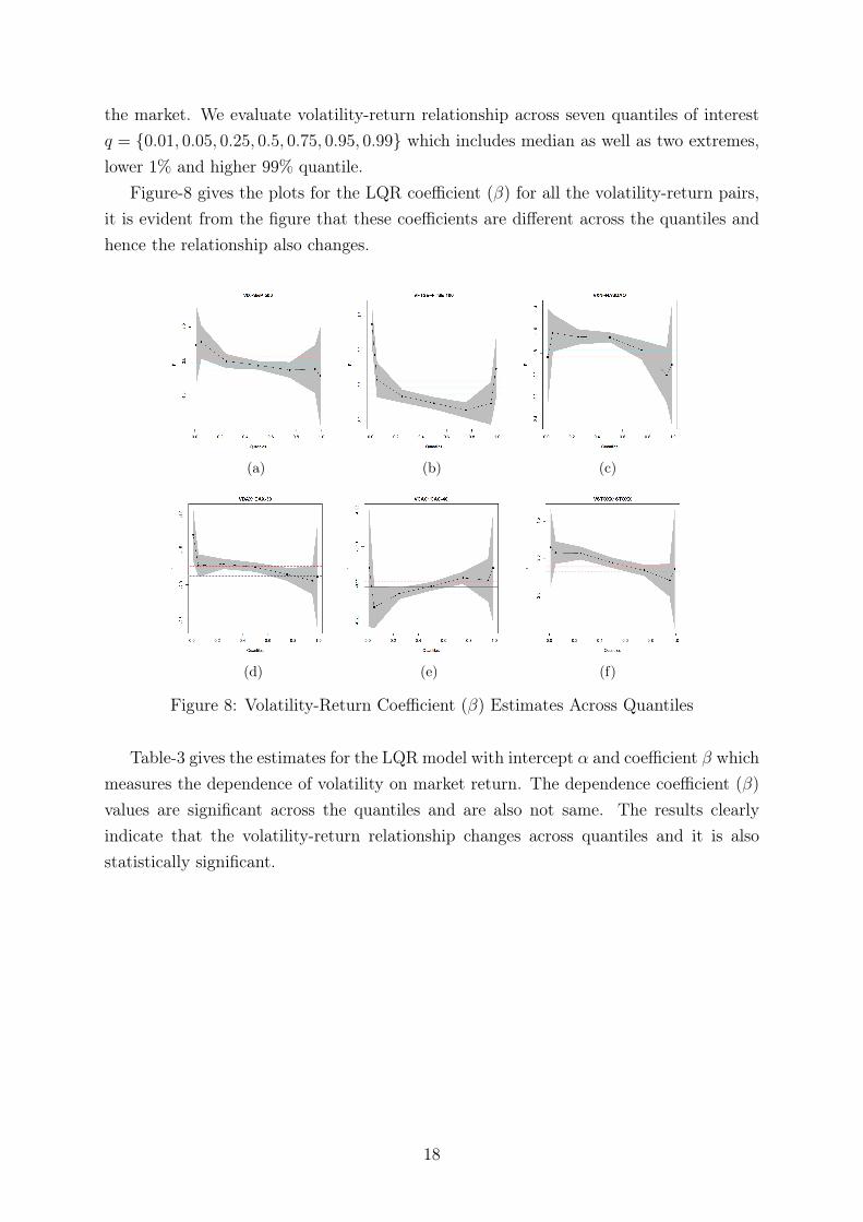
the market. We evaluate volatility-return relationship across seven quantiles of interestq = {0.01, 0.05, 0.25, 0.5, 0.75, 0.95, 0.99} which includes median as well as two extremes,lower 1% and higher 99% quantile.

Figure-8 gives the plots for the LQR coefficient (β) for all the volatility-return pairs,it is evident from the figure that these coefficients are different across the quantiles andhence the relationship also changes.

(a) (b) (c)

(d) (e) (f)

Figure 8: Volatility-Return Coefficient (β) Estimates Across Quantiles

Table-3 gives the estimates for the LQR model with intercept α and coefficient β whichmeasures the dependence of volatility on market return. The dependence coefficient (β)values are significant across the quantiles and are also not same. The results clearlyindicate that the volatility-return relationship changes across quantiles and it is alsostatistically significant.

18

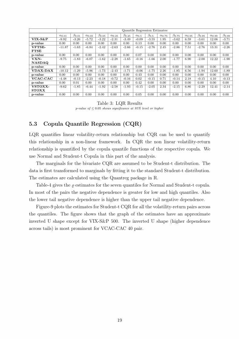
Quantile Regression Estimatesα0.01 β0.01 α0.05 β0.05 α0.25 β0.25 α0.5 β0.5 α0.75 β0.75 α0.95 β0.95 α0.99 β0.99

VIX-S&P -9.92 -3.26 -5.72 -3.22 -2.31 -3.49 -0.09 -3.55 1.95 -3.62 6.59 -3.61 12.06 -3.71p-value 0.00 0.00 0.00 0.00 0.00 0.00 0.13 0.00 0.00 0.00 0.00 0.00 0.00 0.00VFTSE-FTSE

-11.87 -1.63 -6.84 -2.42 -2.63 -2.66 -0.15 -2.76 2.45 -2.86 7.51 -2.76 13.31 -2.26

p-value 0.00 0.00 0.00 0.00 0.00 0.00 0.07 0.00 0.00 0.00 0.00 0.00 0.00 0.00VXN-NASDAQ

-9.75 -1.83 -6.07 -1.62 -2.28 -1.65 -0.16 -1.66 2.00 -1.77 6.90 -2.00 12.22 -1.90

p-value 0.00 0.00 0.00 0.00 0.00 0.00 0.00 0.00 0.00 0.00 0.00 0.00 0.00 0.00VDAX-DAX -10.12 -1.29 -5.96 -1.73 -2.43 -1.71 -0.06 -1.75 2.26 -1.85 6.56 -1.94 12.60 -1.89p-value 0.00 0.00 0.00 0.00 0.00 0.00 0.43 0.00 0.00 0.00 0.00 0.00 0.00 0.00VCAC-CAC -4.48 -0.13 -2.23 -0.18 -0.72 -0.16 0.02 -0.15 0.71 -0.14 2.18 -0.15 4.10 -0.13p-value 0.00 0.01 0.00 0.00 0.00 0.00 0.42 0.00 0.00 0.00 0.00 0.00 0.00 0.00VSTOXX-STOXX

-9.62 -1.85 -6.44 -1.92 -2.58 -1.93 -0.15 -2.05 2.34 -2.15 6.86 -2.29 12.41 -2.14

p-value 0.00 0.00 0.00 0.00 0.00 0.00 0.05 0.00 0.00 0.00 0.00 0.00 0.00 0.00

Table 3: LQR Resultsp-value of ≤ 0.05 shows significance at 95% level or higher

5.3 Copula Quantile Regression (CQR)

LQR quantifies linear volatility-return relationship but CQR can be used to quantifythis relationship in a non-linear framework. In CQR the non linear volatility-returnrelationship is quantified by the copula quantile functions of the respective copula. Weuse Normal and Student-t Copula in this part of the analysis.

The marginals for the bivariate CQR are assumed to be Student-t distribution. Thedata is first transformed to marginals by fitting it to the standard Student-t distribution.The estimates are calculated using the Quantreg package in R.

Table-4 gives the % estimates for the seven quantiles for Normal and Student-t copula.In most of the pairs the negative dependence is greater for low and high quantiles. Alsothe lower tail negative dependence is higher than the upper tail negative dependence.

Figure-9 plots the estimates for Student-t CQR for all the volatility-return pairs acrossthe quantiles. The figure shows that the graph of the estimates have an approximateinverted U shape except for VIX-S&P 500. The inverted U shape (higher dependenceacross tails) is most prominent for VCAC-CAC 40 pair.

19

Normal CQR%0.01 %0.05 %0.25 %0.5 %0.75 %0.95 %0.99

VIX-S&P -0.8645 -0.8913 -0.8861 -0.8916 -0.9099 -0.8696 -0.8602VFTSE-FTSE -0.7735 -0.8114 -0.7925 -0.8137 -0.8287 -0.7891 -0.7497VXN-NASDAQ -0.8066 -0.8164 -0.7647 -0.7045 -0.8047 -0.7831 -0.7718VDAX-DAX -0.7584 -0.7937 -0.7322 -0.7106 -0.7841 -0.7785 -0.7479VCAC-CAC -0.6915 -0.7755 -0.7067 -0.5631 -0.6759 -0.7691 -0.6970VSTOXX-STOXX -0.8015 -0.8055 -0.7517 -0.7496 -0.8122 -0.7999 -0.7469

Student-t CQR%0.01 %0.05 %0.25 %0.5 %0.75 %0.95 %0.99

VIX-S&P -0.8726 -0.8920 -0.8814 -0.8857 -0.9030 -0.8691 -0.8617VFTSE-FTSE -0.7815 -0.8058 -0.7780 -0.7818 -0.8048 -0.7827 -0.7915VXN-NASDAQ -0.8207 -0.8074 -0.7500 -0.6930 -0.7916 -0.7806 -0.7794VDAX-DAX -0.7696 -0.8016 -0.7159 -0.6911 -0.7578 -0.7782 -0.7663VCAC-CAC -0.7868 -0.7608 -0.6436 -0.4888 -0.5959 -0.7667 -0.7661VSTOXX-STOXX -0.8190 -0.8065 -0.7404 -0.7322 -0.7990 -0.8027 -0.7458

Table 4: Normal and Student-t CQR EstimatesAll the estimates given in the table are found to be statistically significant.

Figure 9: Student-t CQR Estimates

Another point of analysis is to see how well the estimates from LQR and CQR fitto the data. Figure-10 plots the LQR and CQR fitted values across the quantiles overthe marginal data. Figure-10(a) plots the VFTSE-FTSE pair fitted values estimatedfrom Normal CQR and LQR and figure-10(b) plots the VIX-S&P pair fitted values esti-

20

mated from Student-t CQR and LQR. The figures show that we can model the non-linearrelationship with the help of copula in quantile regression framework.

(a) VFTSE-FTSE Normal CQR

(b) VIX-S&P Student-t CQR

Figure 10: Fitted Values from CQR and LQR

21

6 Conclusion

The empirical analysis in this paper demonstrated the application of both linear and nonlinear quantile regression models. We used LQR and CQR to model the inverse volatility-return relationship for six volatility-return pairs. The study focussed on the use of copulato model non linear quantile regression which facilitates the quantification of bivariatenon linear correlation within the quantiles of the distribution. Linear regression quantifiesthe relationship between a dependent and independent variable(s) around the mean ofthe distribution and hence does not quantify the relationship for the quantiles across thedistribution. Quantile regression is a very useful tool to quantify the relationship acrossvarious quantiles in a distribution.

Tails of the return distribution are of immense interest in financial risk modelling asthey represent the risk associated with the asset or the financial instrument. Volatility-return relationship and its quantification has importance for hedging as the change involatility leads to the change in market prices. In this analysis we used OLS to quantifythe linear volatility-return relationship around the mean which as quantified by LQR isnot consistent for quantiles across the distribution. CQR is yet another useful tool forquantifying nonlinear bivariate relationship across quantiles. The analysis conducted inthis paper demonstrated that CQR fits better to the actual data than LQR as it is capableof capturing non linear nature of the volatility-return relationship. The results from thisanalysis also supports the asymmetric volatility-return relationship for majority of theindex pairs.

The empirical analysis of this paper has significance for hedging, portfolio managementor risk modelling in general. The empirical analysis in this paper can be furthered byincluding more copula models like Frank Copula, Joe-Clayton copula etc, in CQR model.

Acknowledgements

We thank the Australian Research Council for funding support.

7 References

Alexander, C. (Ed.). (2008). Market Risk Analysis: Practical Financial Econometrics(Vol. II):Wiley Publishing.

Allen, D. E., Gerrans, P., Singh, A. K., and Powell, R. (2009). Quantile Regression and itsapplication in investment analysis. The finsia Journal of Applied Finance (JASSA),7-12.

22

Allen, D., Singh, A. K., & Powell, R. J. (2011). Asset Pricing, the Fama-French factorModel and the Implications of Quantile Regression Analysis. In G. N. Gregoriou &R. Pascalan (Eds.), Financial Econometrics Modeling: Market Microstructure, FactorModels and Financial Risk Measures: Palgrave Macmillan.

Ang, A., & Chen, J. (2002). Asymmetric Correlations of Equity Portfolios. Journal ofFinancial Economics, 63 (3), 443-494.

Badshah, I. U. (2012). Quantile Regression Analysis of the Asymmetric Return-VolatilityRelation. Journal of Futures Markets

Barnes, M. L., & Hughes, W. A. (2002) Quantile Regression Analysis of the Cross Sectionof Stock Market Returns. (Working Paper). Retrieved from Social Science ResearchNework website: http://ssrn.com/abstract=458522

Black, F. (1976) Studies of stock market volatility changes. Proceedings of the AmericanStatistical Association, Business and Economic Statistics Section, 177–81.

Black, F., & Scholes, M. (1973). The pricing of options and corporate liability. Journalof Political Economy, 81, 636–654.

Bouyé, E., & Salmon, M. (2009). Dynamic copula quantile regressions and tail areadynamic dependence in Forex markets. The European Journal of Finance, 15 (7-8),721-750.

Buchinsky, M., Leslie, P., (1997). Educational attainment and the changing U.S. wagestructure: Some dynamic implications. (Working Paper No. 97-13). Department ofEconomics, Brown University.

Buchinsky, M., & Hunt, J. (1999). Wage Mobility In The United States. The Review ofEconomics and Statistics, 81 (3), 351-368.

Campbell, J. Y., & Hentschel, L. (1992). No news is good news: An asymmetric model ofchanging volatility in stock returns. Journal of Financial Economics, 31 (3), 281-318.

Christie, A. (1982). The stochastic behaviour common stock variances: Value, leverageand interest rate effects. Journal of Financial Economics, 10, 407–432.

23

Chan, L. K. C., & Lakonishok, J. (1992). Robust Measurement of Beta Risk. The Jour-nal of Financial and Quantitative Analysis, 27 (2), 265-282.

Cheung, W. (2009). Copula: A Primer for Fund Managers. SSRN eLibrary.

Clayton, D. (1978). A model for association in bivariate life tables and its application inepidemiological studies of familial tendency in chronic disease incidence. Biometrika,65, 141–151.

Dennis, P., Mayhew, S., and Stivers, C (2006). Stock returns, implied volatility innova-tions, and the asymmetric volatility phenomenon. Journal of Financial and Quanti-tative Analysis, 41 (2), 381-406.

Eide, E., & Showalter, M. H. (1998). The Effect of School Quality on Student Perfor-mance: A Quantile Regression Approach. Economics Letters, 58 (3), 345-350.

Engle, R. F., & Manganelli, S. (2004). CAViaR: Conditional Autoregressive Value at Riskby Regression Quantiles. Journal of Business & Economics Statistics, 22 (4), 367-381.

Erb, C. B., Harvey, C. R., & Viskanta, T. E. (1994). Forecasting International EquityCorrelations. Financial Analysts Journal, 50, 32-45.

Fleming, J., Ostdiek, B., & Whaley, R. E. (1995). Predicting stock market volatility: Anew measure. Journal of Futures Markets, 15 (3), 265-302.

Franke, J., Härdle, K. W., & Hafner, C. M. (2008) . Statistics of Financial Market: AnIntroduction (II ed.): Springer-Verlag Berlin Heidelberg.

Gowlland, C., Xiao, Z. Zeng, Q. (2009). Beyond the Central Tendency: Quantile Re-gression as a Tool in Quantitative Investing. The Journal of Portfolio Management,35 (3), 106-119.

Giot, P., (2005). Relationships between implied volatility indices and stock index returns.Journal of Portfolio Management, 31, 92-100.

Hibbert, A., Daigler, R., & Dupoyet, B. (2008). A behavioural explanation for thenegative asymmetric return-volatility relation. Journal of Banking and Finance 32,2254-2266.

Joe, H. (Ed.). (1997). Multivariate Models and Dependence Concepts : Chapman andHall.

24

Koenker, R. W., & Bassett, G. Jr. (1978). Regression Quantiles. Econometrica 46 (1),33-50.

Koenker, R. (2005). Quantile Regression, Econometric Society Monograph Series: Cam-bridge University Press.

Kumar, S. S. S. (2012). A first look at the properties of India’s volatility index. Interna-tional Journal of Emerging Markets, 7 (2),160 - 176.

Liu, J., Pan, J., & Wang, T. (2005). An equilibrium model of rare-event premia and itsimplication for option smirks. Review of Financial Studies, 18, 131-164.

Longin, F., & Solnik, B. (2001). Extreme correlation of international equity markets.Journal of Finance 56, 649-676.

Low, C. (2004). The fear and exuberance from implied volatility of S&P 100 index op-tions. Journal of Business 77, 527-546.

Morillo, Daniel. (2000). Income Mobility with Nonparametric Quantiles: A Comparisonof the U.S. and Germany. Preprint.

Nelsen, R. B. (1999). Introduction to Copulas : Springer Verlag.

Patton, A. J. (2004). On the Out-of-Sample Importance of Skewness and AsymmetricDependence for Asset Allocation. Journal of Financial Econometrics 2 (1), 130-168.

Copula-Based Models for Financial Time Series, 2009, in T.G. Andersen, R.A. Davis, J.-P. Kreiss and T. Mikosch (eds.) Handbook of Financial Time Series, Springer Verlag.

Whaley, R. (2000). The investor fear gauge. Journal of Portfolio Management 26, 12-17.

Wu, G. (2001). The Determinants of Asymmetric Volatility. The Review of FinancialStudies, 14 (3), 837-859.

25