COMBINED PENALIZED QUANTILE REGRESSION IN HIGH DIMENSIONAL MODELS
22
© 2015 Pakistan Journal of Statistics 49 Pak. J. Statist. 2015 Vol. 31(1), 49-70 COMBINED PENALIZED QUANTILE REGRESSION IN HIGH DIMENSIONAL MODELS Muhammad Amin § , Lixin Song § , Milton Abdul Thorlie and Xiaoguang Wang School of Mathematical Sciences, Dalian University of Technology Dalian, 116023, P.R. China § Corresponding authors Email: [email protected], [email protected] ABSTRACT The quantile regression technique is considered as an alternative to the classical ordinary least squares (OLS) regression in case of outliers and heavy tailed errors existing in linear models. In this work, the consistency, asymptotic normality, and oracle property are established for sparse quantile regression with a diverging number of parameters. The rate of convergence of the combined penalized estimator is also established. Furthermore, the rank correlation screening (RCS) method is applied to deal with an ultrahigh dimensional data. The simulation studies, the analysis of hedonic housing prices and the demand for clean air dataset are conducted to illustrate the finite sample performance of the proposed method. KEYWORDS Combined penalization; Ridge-SCAD; Variable selection; Quantile regression. 1. INTRODUCTION The existence of heavy tailed error or outliers (response or predictors) in linear models restrict the use of classical regression techniques. The present variable selection methods of linear regression models based on Ridge-SCAD regression are only applicable for the finite number of predictors and most of them lack the oracle property associated with the estimator. The traditional variable selection methods have several drawbacks, the most important is that they are unstable due to their inherent discreteness (Breiman, 1996). To overcome such drawbacks some shrinkage procedures based on the penalized function have been proposed, which include the bridge regression (Frank and Friedman, 1993) and the smoothly clipped absolute deviation (SCAD) (Fan and Li, 2001). Various penalized approaches have been proposed for exploring the selection of variables and explaining the statistical properties of high dimensional data. Huang et al. (Huang, Horowitz and Ma, 2008) studied variable selection in the accelerated failure time model via the bridge penalty. Ma and Du (2012) studied the variable selection in the partially linear model with high dimensional covariates. The 1 L penalty that yields the soft threshold rule (Donoho and Johnstone, 1994) and leads to the least absolute shrinkage and selection operator (Lasso) which was introduced by Tibshirani (1996), the same was further studied by Efron et al. (2004). The 2 L penalty which resulted in the ridge regression was discussed by Hoerl and Kennard (1970). Zou and Hastie (2005)
Transcript of COMBINED PENALIZED QUANTILE REGRESSION IN HIGH DIMENSIONAL MODELS
© 2015 Pakistan Journal of Statistics 49
Pak. J. Statist.
2015 Vol. 31(1), 49-70
COMBINED PENALIZED QUANTILE REGRESSION
IN HIGH DIMENSIONAL MODELS
Muhammad Amin
§, Lixin Song
§, Milton Abdul Thorlie and Xiaoguang Wang
School of Mathematical Sciences, Dalian University of Technology Dalian, 116023, P.R. China
§Corresponding authors Email: [email protected], [email protected]
ABSTRACT
The quantile regression technique is considered as an alternative to the classical ordinary least squares (OLS) regression in case of outliers and heavy tailed errors existing in linear models. In this work, the consistency, asymptotic normality, and oracle property are established for sparse quantile regression with a diverging number of parameters. The rate of convergence of the combined penalized estimator is also established. Furthermore, the rank correlation screening (RCS) method is applied to deal with an ultrahigh dimensional data. The simulation studies, the analysis of hedonic housing prices and the demand for clean air dataset are conducted to illustrate the finite sample performance of the proposed method.
KEYWORDS
Combined penalization; Ridge-SCAD; Variable selection; Quantile regression.
1. INTRODUCTION
The existence of heavy tailed error or outliers (response or predictors) in linear models restrict the use of classical regression techniques. The present variable selection methods of linear regression models based on Ridge-SCAD regression are only applicable for the finite number of predictors and most of them lack the oracle property associated with the estimator. The traditional variable selection methods have several drawbacks, the most important is that they are unstable due to their inherent discreteness (Breiman, 1996). To overcome such drawbacks some shrinkage procedures based on the penalized function have been proposed, which include the bridge regression (Frank and Friedman, 1993) and the smoothly clipped absolute deviation (SCAD) (Fan and Li, 2001). Various penalized approaches have been proposed for exploring the selection of variables and explaining the statistical properties of high dimensional data. Huang et al. (Huang, Horowitz and Ma, 2008) studied variable selection in the accelerated failure time model via the bridge penalty. Ma and Du (2012) studied the variable selection in the
partially linear model with high dimensional covariates. The 1L penalty that yields the
soft threshold rule (Donoho and Johnstone, 1994) and leads to the least absolute shrinkage and selection operator (Lasso) which was introduced by Tibshirani (1996), the
same was further studied by Efron et al. (2004). The 2L penalty which resulted in the
ridge regression was discussed by Hoerl and Kennard (1970). Zou and Hastie (2005)

Combined Penalized Quantile Regression in High Dimensional Models 50
proposed the elastic net (Enet) method, which is a combination of Lasso and ridge penalties.
The quantile regression method proposed by Koenker and Bassett (1978) has attracted
much attention as an alternative approach to least square regression. A comprehensive
introduction and recent important developments are studied by Koenker (2005). It is a
flexible technique in assessing the effect of predictors on different locations of the
response distribution. He and Shao (2000) established the asymptotic theory for high
dimensional M-regression with non-smooth objective function. The results of which can
be applied to quantile regression without assuming sparseness assumption.
Wang et al. (2010) proposed a new combined penalization in the linear regression
which outperforms the SCAD penalty especially when the correlation among the
predictors is high. In this article, the methodology and the theory of quantile regression
for variable selection via Ridge-SCAD regression considering high dimensional
regression setting in which the number of covariates '' ''p grows at an increasing rate of
the sample size '' ''n is further extended.
Furthermore, we demonstrated that under certain asymptotic conditions, the combined
penalized quantile estimator with properly selected tuning parameters satisfies the oracle
property. The rank correlation screening (RCS) method proposed by Li et al. (2012) is
required to deal with ultrahigh dimensional data.
The rest of this article is organized as following. Section 2 introduces the estimation
and the combined penalty quantile selection procedure in a high-dimension and it also
presents the theoretical results. The simulation studies and the numerical comparisons are
given in Section 3. All the technical proofs of theorems are given in Section 4. Section 5
concludes the article with a discussion.
2. COMBINED PENALIZED QUANTILE REGRESSION
2.1 Ridge-SCAD Estimation and Variable Selection Procedure
If we consider linear regression model
0 , 1, ,i i iY x i n
(1)
where iY is the response variable, 0 is the vector of regression coefficients, ix is a
random vector of predictors np and i is the random error with median zero. Without
loss of generality, it is assumed that the outcome is centered and the predictors are
standardized. Theerefore, interncept 0 is excluded in the regression model. The model
is sparse given by 0 10 20, ,
in which 10 0 is a 1nk vector and 20 = 0 is a
1nm vector. For = ,n n np k m where nk & nm are the significant and non significant
predictors accordingly. The error term satisfies 0 |i ip x for 0 < 1 . Let
0= 1 , 0n jA j p is a set of nonzero coefficients. The oracle estimator is defined

Amin, Song, Thorlie and Wang 51
as 0 10 20ˆ ˆ ˆ, ,
where 10̂ is the combined quantile regression estimator when the
model is fitted using covariants in set A. The recent literature reveals that various
versions of penalized functions are proposed for high dimensional data. Belloni and
Chernozhukov (2011) derived an error bound for quantile regression corresponding to
1L -penalty to reduce the quantile regression bias but it lacks the oracle property. The
bridge penalty was proposed by Frank and Friedman (1993) regarding qL -penalty
defined as | | = | | , 0 < < 1qp q . Knight and Fu (2000) investigated the asymptotic
nature of bridge estimators for finite number of covariates. Fan and Li (2001) discussed
the SCAD penalty, given by
22 21 | || | | | 0 | | | |
2 1
a ap I I a
a
21
| |2
aI a
(2)
where = 3.7a and > 0 is the tuning parameter. It is continuous and differentiable on
,0 0, but not differentiable at zero. It’s derivative vanishes outside ,a a .
An alternative combined quantile (ridge and SCAD) strategy is proposed. For any fixed
non-negative value of and , the combined penalty can be written as:
2, ( ) ( ) ( ), 0.
2J P
If we consider a combined penalized quantile high dimensional regression model
given by
2
1 1
1| | ,
2
pn nn
n n i n i nj njn ni j
Q Y x Pn
(3)
where ( ) 0m m I m is a quantile check function. (.)n
P and (.)n are the
functions of SCAD and ridge penalization. The n and n are non-negative tuning
parameters of SCAD and ridge penalties and are responsible to control the model
complexity with given rates. Combined penalized estimator can be minimized as
2
1 1
1| | ,
2
pn nn
i n i nj njn ni j
Y x Pn
This minimization problem can be expressed as a constraints to smoothen the
optimization problem. In optimization, these constraints will lead to asymptotic aspect
of the Ridge-SCAD penalized regression under the given conditions. In order to
significantly improve computational efficiency of the model, we consider the objective
function given by
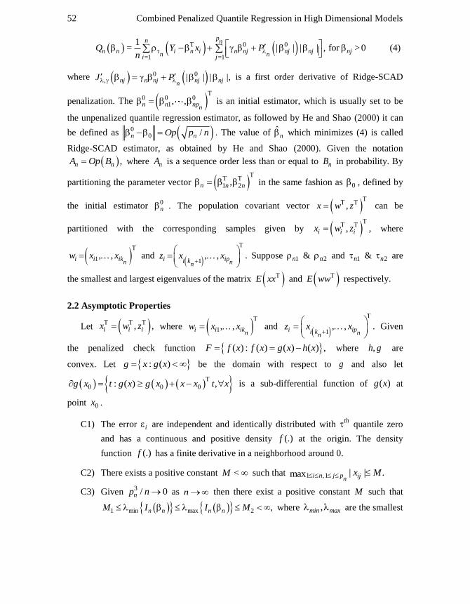
Combined Penalized Quantile Regression in High Dimensional Models 52
0 0
=1 =1
1= | | | | , for >0
pn n
n n i n i n nj nj nj njn ni j
Q Y x Pn
(4)
where 0 0, | | | |,nj n nj nj nj
nJ P is a first order derivative of Ridge-SCAD
penalization. The 0 0 01, ,n n np
n
is an initial estimator, which is usually set to be
the unpenalized quantile regression estimator, as followed by He and Shao (2000) it can
be defined as 00 /n nOp p n . The value of ˆ
n which minimizes (4) is called
Ridge-SCAD estimator, as obtained by He and Shao (2000). Given the notation
,n nA Op B where nA is a sequence order less than or equal to nB in probability. By
partitioning the parameter vector 1 2,n n n
in the same fashion as 0 , defined by
the initial estimator 0n . The population covariant vector ,x w z
can be
partitioned with the corresponding samples given by , ,i i ix w z
where
1, ,i i ikn
w x x
and 1
, ,i ipi k nn
z x x
. Suppose 1n & 2n and 1n & 2n are
the smallest and largest eigenvalues of the matrix E xx and E ww respectively.
2.2 Asymptotic Properties
Let , ,i i ix w z where 1, ,i i ik
nw x x
and 1
, , .i ipi k nn
z x x
Given
the penalized check function ( ) : ( ) ( ) ( ) ,F f x f x g x h x where ,h g are
convex. Let : ( )g x g x be the domain with respect to g and also let
0 0 0: ( ) ,g x t g x g x x x t x
is a sub-differential function of ( )g x at
point 0x .
C1) The error i are independent and identically distributed with th quantile zero
and has a continuous and positive density (.)f at the origin. The density
function (.)f has a finite derivative in a neighborhood around 0.
C2) There exists a positive constant <M such that 1 ,1 | | .max i n j p ijnx M
C3) Given 3 / 0np n as n then there exist a positive constant M such that
1 min max 2 ,n n n nM I I M where ,min max are the smallest

Amin, Song, Thorlie and Wang 53
and largest eigenvalues respectively. Given 1 = / ,i n i p n nmax z O p n a
where max , ,1n nj nj na j p ,j j are the functions of n .
C4) There exist constants 1 20 < < < and 1 20 < < < such that
1 1 2 2n n and 1 1 2 2n n .
C5) The true model dimension satisfies 0n for / ,n n nn p n
and 0,nn as n .
The condition (C1) is typical and widely employed in the literature (Knight, 1998;
Pollard, 1991; Wu and Liu, 2009), (C2) explains the restriction on covariates and defines
the properties of consistency and asymptotic normality. It requires design matrix
corresponding to the true model if it is well behaved. The same one was used by Huang
and Xie (2007). The (C3) express that 1/3np o n and the same was taken by Huber
(1973), (C4) assume the matrices TE xx and TE ww are positive definite and is
identical to the condition given in Huang et al. (2008) and Li et al. (2011). In particular
they are similar to Kim et al. (2008). Condition (C5) ensures the estimator with sparsity
property by Fan and Peng (2004).
Theorem 2.2.1 (Consistency)
Under conditions (C1) to (C5), 0ˆ / ,n P n nO p n a it shows the consistent
estimator for true parameter 0 with optimal convergence rate regarding diverging
number of parameters.
We partition 1 2ˆ ˆ ˆ, ,
TT T
n n n given 0 . Let 1 10=n n and 1 10ˆ ˆ= ,n n we have
a new function, * 010
=1 =1
1= w | | | | .
kn nT
n n i n i n nj nj nj jni j
Q Pn
Let
Tn ng w , then linear approximation near 0 is
(0) (0) ,n n n ng g D r
where (0) 0 0D I I w , ( )I is the indicator function, and nr is the
remainder term. Let 1
1 n
n n i n ii
S wn
and n nS E w . Then
| .n n nS E E w w E H w
Given

Combined Penalized Quantile Regression in High Dimensional Models 54
0i n iw
where 1
= , 1 .ij
w j p
=1
| =n
n n Ti n i ij n j nj
inj
QY x x w sgn
Suppose ( )H has a finite third order derivative, then the empirical process nE
defined by ( ) = ( ) ( )n nE n S S given (.) therefore ( ) = ( 0) (1 ) | ( < 0)it t t
and let ,11.nE ww
Theorem 2.2.2 (Oracle Property)
Suppose that 3 3 / 0n nk p n , ˆ 1/n n P nE r o p , / / 0n np n , and 0.nn
If the conditions (C1)-(C5) hold, the Ridge-SCAD estimator 1 2ˆ ˆ ˆ,n n n
satisfies
(1) Sparsity: 2ˆPr 0 1 as .n n
(2) Asymptotic normality: 21/2 1/2,11 1 10
ˆ 0, 1 (0) ,D
n nn N f
where is an arbitrary 1nk vector with = 1 , D
means convergence in
distribution.
2.3 Computation and Selection of Tuning Parameters
By following the similar idea of computation proposed by Wang et al. (2012), the
objection function in (4) can be minimized as
( 1)
1 1
1min
pn nT t
i nj i j ji j
Y x wn
where ( 1) ( 1) ( 1) 0t t tj n j n jw P
. Given , and n n j , and with the aid of
slack variables, the convex optimization problem above can also be casted into a
constrained linear programming problem as follows
( 1)
, 1 1
1(1 )min
pn nt
i i j ji j
wn
subject to = ; = 1,2, , ,Ti i i nj iY x i n
0, 0; =1,2, , ,i i i n
, ; =1,2, , .j j j j j p

Amin, Song, Thorlie and Wang 55
This minimization can be achieved by using any existing linear programming
software, we use the R function . .rq fit fn in the package .quantreg
In order to deal with the ultrahigh dimensional case, we first reduce the
dimensionality from >>np n to <np n and applied RCS method originally proposed by
Li et al. (2012). Let 1= , , pn
w w w
be a np -vector, where
1 1
, 1, , .( 1) 4
n
k ik jk i j ni j
w I x x I y y k pn n
where (.)I denotes the indictor function, and w is the marginal rank correlation
coefficient. The np which is a magnitudes of the vector w is sorted in a decreasing order
to define the submodel,
1 :| | is among the first largest of all ,n k nk p w d
the method is relatively simple, since it shrinks the full model 1, , np to a submodel
with size <nd n .
Several selection criterias such as cross validation (CV), generalized cross validation
(GCV), Akaike information criterion (AIC) and Bayesian information criterion (BIC) can
be used to choose proper tuning parameters. BIC-type criterion was used that is given in
the following formula which was also used in Jiang et al. (2014).
=1
1 log( )ˆ( ) = log x ( ),n
i ii
nBIC Y edf
n n
where the first term measures the quadratic loss and edf as the number of nonzero
coefficients.
3. NUMERICAL STUDIES
This section illustrates the finite sample performance of the proposed method. It
mainly focuses on comparing the performance of the combined Ridge-SCAD (CP)
method with Lasso, Enet and SCAD. A real data set is used for further demonstration.
Example 3.1
The data simulated from linear model is,
= x ,Y
with “ n ” observations. is a 1np vector with 1 2 5= 3, =1.5, = 2 and the other
j ’s being 0. The vector of covariates “ x ” follows a multivariate normal distribution
0, ,xN | |i jx ij
r for 1 , ni j p with r=0.5. To emphasize the dependency of the

Combined Penalized Quantile Regression in High Dimensional Models 56
number of parameters on the sample size, we considered =100n with 1/4= 10np n .
For comparison, three error distributions are studied: the standard normal distribution, the
t -distribution with 3 d.f, and the contaminated standard normal (CN) distribution with
10% outliers from the standard cauchy distribution. With model error, the finite
performance of Qr.Lasso, Qr.Enet, Qr.SCAD, quantile Combined Penalization (Qr.CP)
and Oracle compared. The oracle estimator is computed by using the true model
when the zero coefficients are known, in practice, it cannot be obtained. It can only
be used here as a benchmark for comparison. The model error is computed by
xˆ ˆ= .n nME
The results of the variable selection and the model errors are
summarized in Table 1. The column “MRME" stands for the median of the relative
model error, which is defined as the ratio of ME to MEL, where ME is the model error of
a selected model, and MEL is the model error of the proposed estimate under the full
model. "C” denotes the average number of zero coefficients correctly set to zero, and
“IC” gives the average number of nonzero coefficients incorrectly set to zero. Table 1
shows that Qr.CP and Qr.SCAD are very close to oracle in terms of MRME in all error
distributions, but the others performed worse. The Qr.CP and Qr.Enet are better than
Qr.SCAD and Qr. Lasso, respectively. Overall Qr.CP and Qr.SCAD are one of the best
variable selectors among the penalization methods in this example.
Table 1
Simulation Results with 1000 Data Sets 100, 31nn p
Methods (0,1)N (3)t CN
C IC MRME C IC MRME C IC MRME
0.3
Qr.Lasso 26.43 0.000 0.2998 26.70 0.016 0.2696 26.76 0.012 0.3244
Qr.Enet 26.45 0.000 0.2988 26.79 0.013 0.2674 26.80 0.012 0.3199
Qr.SCAD 27.88 0.000 0.0664 27.82 0.016 0.0639 27.93 0.012 0.0545
Qr.CP 27.88 0.000 0.0663 27.83 0.012 0.0629 27.95 0.003 0.0541
Oracle 28.00 0.000 0.0551 28.00 0.000 0.0439 28.00 0.000 0.0507
0.5
Qr.Lasso 26.69 0.000 0.3247 27.01 0.004 0.3082 26.98 0.006 0.3339
Qr.Enet 26.73 0.000 0.3247 27.07 0.005 0.3059 27.01 0.006 0.3328
Qr.SCAD 27.92 0.000 0.0664 27.91 0.012 0.0582 27.97 0.001 0.0537
Qr.CP 27.92 0.000 0.0662 27.92 0.007 0.0572 27.97 0.007 0.0542
Oracle 28.00 0.000 0.0598 28.00 0.000 0.0467 28.00 0.000 0.0519
0.7
Qr.Lasso 26.46 0.002 0.2999 26.57 0.012 0.2621 26.70 0.012 0.3129
Qr.Enet 26.46 0.002 0.2946 26.65 0.008 0.2619 26.76 0.012 0.3098
Qr.SCAD 27.85 0.000 0.0686 27.81 0.018 0.0601 27.93 0.01 0.0579
Qr.CP 27.86 0.000 0.0685 27.82 0.022 0.0599 27.95 0.003 0.0574
Oracle 28.00 0.000 0.0567 28.00 0.000 0.0444 28.00 0.000 0.0552
Amin, Song, Thorlie and Wang 57
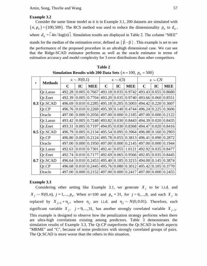
Example 3.2
Consider the same linear model as it is in Example 3.1, 200 datasets are simulated with
, = 100,500nn p . The RCS method was used to reduce the dimensionality np to nd ,
where = 4 / log( ) .nd n n Simulation results are displayed in Table 2. The column “MEE”
stands for the median of the estimation error, defined as ̂ . This example is set to see
the performance of the proposed procedure in an ultrahigh dimensional case. We can see
that the Ridge-SCAD estimator performs as well as the oracle estimator in terms of
estimation accuracy and model complexity for 3 error distributions than other competitors.
Table 2
Simulation Results with 200 Data Sets 5 0100, 0npn
Methods (0,1)N
(3)t
CN
C IC MEE C IC MEE C IC MEE
0.3
Qr.Lasso 492.28 0.005 0.7667 493.18 0.035 0.9742 493.43 0.055 0.8680
Qr.Enet 492.39 0.005 0.7704 493.20 0.035 0.9740 493.66 0.060 0.8551
Qr.SCAD 496.69 0.010 0.2285 495.18 0.205 0.5003 494.42 0.220 0.3607
Qr.CP 496.76 0.010 0.2269 495.39 0.140 0.4744 496.24 0.225 0.3606
Oracle 497.00 0.000 0.2056 497.00 0.000 0.2185 497.00 0.000 0.2122
0.5
Qr.Lasso 493.42 0.005 0.7248 493.82 0.030 0.8443 494.39 0.020 0.8435
Qr.Enet 493.31 0.005 0.7197 494.05 0.030 0.8368 494.47 0.020 0.8416
Qr.SCAD 496.79 0.005 0.2134 495.54 0.095 0.3964 496.08 0.160 0.2903
Qr.CP 496.80 0.005 0.2124 495.78 0.055 0.3813 496.41 0.090 0.2872
Oracle 497.00 0.000 0.1950 497.00 0.000 0.2145 497.00 0.000 0.1944
0.7
Qr.Lasso 492.63 0.010 0.7301 492.41 0.055 1.0121 492.92 0.035 0.8477
Qr.Enet 492.74 0.010 0.7177 492.69 0.065 0.9566 492.85 0.035 0.8445
Qr.SCAD 496.64 0.010 0.2453 495.40 0.185 0.3215 494.00 0.145 0.3874
Qr.CP 496.68 0.010 0.2445 495.76 0.080 0.3012 495.42 0.105 0.3770
Oracle 497.00 0.000 0.2152 497.00 0.000 0.2417 497.00 0.000 0.2455
Example 3.3
Considering other setting like Example 3.1, we generate jX to be i.i.d. and
(0, ), =1,..., .j nX N n j p When n=100 and = 31,np for = 6,...,8,j and each jX is
replaced by 3 ,j jX where j are i.i.d. and (0,0.01).j N Therefore, each
significant variable ,jX = 9,...,31,j has another strongly correlated variable 3.jX
This example is designed to observe how the penalization strategy performs when there
are ultra-high correlations existing among predictors. Table 3 demonstrates the
simulation results of Example 3.3, The Qr.CP outperforms the Qr.SCAD in both aspects
"MRME" and "C", because of noise predictors with strongly correlated groups of pairs.
The Qr.SCAD is more worse than the others in this situation.

Combined Penalized Quantile Regression in High Dimensional Models 58
Table 3
Simulation Results with 200 Data Sets 100, 31nn p
Methods 0.3 0.5 0.7
C IC MRME C IC MRME C IC MRME
Qr.Lasso 26.17 0 0.0018 26.61 0 0.0026 26.02 0 0.0020
Qr.Enet 26.26 0 0.0016 26.77 0 0.0023 26.19 0 0.0019
Qr.SCAD 22.39 0 0.6072 22.47 0 0.7593 22.24 0 0.6456
Qr.CP 27.55 0 0.0002 27.56 0 0.0002 27.46 0 0.0002
Oracle 28.00 0 0.0001 28.00 0 0.0001 28.00 0 0.0001
Example 3.4
To examine the usefulness of proposed method, It was applied to analyze a data set of
the Boston housing data to examine the correlation between clean air and housing prices
(Harrison and Rubinfeld, 1978). There are 506 observations, 13 independent factors, and
a response variable LMV, which is the logarithm of the median value of owner-occupied
homes. Details are available online at http://lib.stat.cmu.edu/datasets/dostoncorrected.txt.
Linear model to the LMV after first standardizing the predictors is fitted. The Q-Q plot
and box plot showed that the response variable LMV contains many obvious outliers.
Therefore, application of the penalized quantile regression is much better than penalized
OLS approach. We split 506 observations into first 400 observations as a training data set
to select and fit the model, and rest as a testing data set to evaluate the prediction ability
of the selected model. Then was calculated the median absolute prediction error (MAPE)
ˆmedian | |, =1,...,106i iy y i using the testing data. The performance of the penalized
quantile regression with different penalties and different quantiles are summarized in
Table 4. The results indicate that Qr.CP and Qr.SCAD select the simplest model, while
Qr.Lasso and Qr.Enet include extra variables.
Table 4
Results of the Boston House Price Data
Methods 0.3 0.5 0.7
No. Zeros MAPE No. Zeros MAPE No. Zeros MAPE
OLS 0 5.3147 0 5.3147 0 5.3147
QR. 0 3.0460 0 3.0835 0 3.2543
Qr.Lasso 5 3.3552 5 3.1569 5 3.1896
Qr.Enet 5 3.2641 6 3.1684 5 3.1248
Qr.SCAD 10 3.0339 8 3.0506 6 3.0521
Qr.CP 10 3.0213 8 3.0578 6 3.0124

Amin, Song, Thorlie and Wang 59
4. PROOF OF THEOREMS
Proof of Theorem 2.2.1:
With any given > 0, there exist a constant C such that
0 0=
Pr > 1 ,inf n n nu C
Q u Q
(5)
where /n n np n a which implies that probability at least 1 , there exist a
local minimum in the ball 0{ : },nu u C where u is a 1np vector, that
is there exists a local minimizer such that 0ˆ = /n P n nO p n a . Let
0 0( ) ,n n n nD u Q u Q then
0 0=1 =1
1 1( ) = u
n n
n i n i i ii i
D u Y x Y xn n
0 0=1
upn
n j n j jj
0
01
| | | |pn
nj j n j njn nj
p u p
0=1
1= u
n
i n ii
Y xn
00 0
=1
u | | | u |pn
n j n j n nj j n jj
p
00 0 0
=1 =1
1| | | |
pn n
i i n j nj jni j
Y x pn
0
=1 =1 =1
1u u | | | u |
k kn n n
i n i i n n j nj n jni j j
x pn
1 2 3.n n nI I I
According to Knight (1998), it holds that for 0x we have
0
| | | |= ( > 0) ( < 0) 2 ( ) ( 0) ,y
x y x y I x I x I x s I x ds
Applying this equation, we can expand
/
0| | | |= ( >0) ( <0) 2 ( ) ( 0)
p n a u xn n ix y x y I x I x I x s I x ds
First, we consider the term 1In , we have
Combined Penalized Quantile Regression in High Dimensional Models 60
1
1
10 0
n
n n i i ii
I u x I In
/
01
20
n p n a u xn n i
i ii
I s I dsn
11 12I In n
By condition C(4) using central limit theorem, 11
nI converges in distribution then
iu x , ix is a p-dimensional random vector with mean zero and =iCov x and if 3nI
converges to real function u in probability denoted by cumulative distribution function
of i then, we obain
u
0> 0 < 0 ,
xn i
i iI I ds
and
2
22
211 =1
I = u u > 0 < 0n
nn i i i i
i
Var E x x E I In
2 2
2 2 22= u u u .n n
i i nE x xn n
By Markov Inequality, 2 2 2 2
2112 2
2 4 4 2 4 411
I / uPr | I | 0,
n n n
n n
n n
E nK
K K
which implies 2 2
11I = .n P no Considering the second term of 1nI which gives
12nI , if
its converges to a real function u then we get,
u
0> 0 < 0 (u ),
xn i
i i niI I ds by Z u
hence,
12 13 14=1 =1 =1
I = I In n n
n ni ni ni ni n ni i i
Z Z E Z E Z
Since
2
2 | |2
02
4 4( ) 0 0
u xn i
ni i iE Z u I I ds E dsnn
2 2 2
2 2 2 2 22
4= | u |
4 4u u u ,
n i
n i i n n
E xn
E x xn n
Given that there exist a constant function f , > 0 and 0 < < ,k therefore
| |<( ) < (0)sup x
f x f k
, then we have
Amin, Song, Thorlie and Wang 61
24
= (u) | u | <ni n iE Z I xn
|u |
0
40 | | <
xn i
i i n iI s I ds I u xn
|u |
0
4(0) | u | <
xn i
n if k E sds I xn
2 2 24
(0) | u |n if k E xn
From the dominated convergence theorem, when given expression converges to zero
as 0 then it follows that as ,n 2=1 =1
4= (u) 0,n n
ni ni nii iVar Z Var Z Zn
we have, 2 2=1 (u) (u) =n
ni ni ni Z E Z op , then 2 2
14I = .n nop
By Markov Inequality, from conditions C(2)-C(3), we obtain
* *
1 =1
Pr | u | > = Pr | u |>maxn
n i n ii n i
x x
*1Pr | u |>nn x
6 66
16*unn E x
36 6 3
2 6*
10,n
n
pC p
n
which gives us, 1 | u | = (1).max i n n i Px o
015
I = = 2 0u x
n in ni i inZ E I s I ds
0
= 2 ( ) (0)x
n iE E F s F ds
2= (0) 1 (1) u u.n i if E o E x x
Consider 2I ,n u is large enough, 1 < 0nI , we have
2
=1
| I |=| |kn
n n n jj
u 2= unn
n
2 u ,nOp for 3In , we have
0
3=1
| I |=| | ) | | | u |kn
n n nj nj n jnj
p sgn 0
=1
| | | | | u |kn
n nj nj n jnj
p sqn
un n nk a 2 un
From condition C(5), we have 23I = un nOp . It can be followed from the law of
large numbers that =1 (u) , " "nnii Z p p convergence in probability then the right
Combined Penalized Quantile Regression in High Dimensional Models 62
hand side of 1In converges to 2 2(0)(1 (1)) unf o in probability. By condition C(5),
we get
0 * 0
j jPr | | u > Pr | | | | u < ,n nj nj nj nj nn
n p sgn I a
for * > 0 , we can have 0
j| | u = (1).njn
n p op By condition C(1), choosing large
value C , which is uniform then =u C and ( )nD u converges to 0, hence the terms 1In
and 2In are dominated by 3In which is positive, therefore this satisfies our proof.
To facilitate the proof of the Theorem 2.2.2, the following Lemma 4.1 is needed,
which indicates that under certain conditions, the proposed estimator has the sparsity
property, i.e. the insignificant variables can exactly be estimated by zero with probability
approaches to one.
Lemma 4.1:
Under conditions (C1) to (C5), the estimator 1 2ˆ ˆ ˆ= ,n n n
satisfies
2ˆPr = 0 1.n
Proof:
By following Theorem 2.2.1, for a sufficiently large ,C ˆn lies in the ball
0: nC with probability converging to 1, where = / .n n np n a Let
1 10 1=n nu and 2 20 2 2= =n n nu u , where 2 2 2 2
1 2= ,u u u C we
obtain 0=1
1=
n
j n ij i ii
S X Y xn
for ˆ, where = 0n j nj p S satisfies the
oracle estimator. 0Pr | |nj na for = 1,2, , 1.nj p Let 1 2,nH u u , given
u C and if 2 > 0u then the minimizer 1 2,nH u u over u C converges to 0,
hence 1 2 1, ,0 > 0n nH u u H u with probability converging to 1. Note That,
1 2 1, ,0n nH u u H u
1 2 10 1 10= , ,0 ,0 ,0n n n n n n nQ Q Q Q
1 2
=1 =1
1 1= w z
n n
i n i n i ii i
u un n
1
=1 =1
1 1w
n n
i n i ii i
un n
02
=1
| | | | .m
n
n nj nj n jnj
P u

Amin, Song, Thorlie and Wang 63
By condition C(4), we have 2 2iPr | z |> = nt op for > 0 hence
iPr | z |> /n np n a , for some, =1,2, , ni p
2 2
i=1
| z |>pn
ni
2 21= n np
2 210n
1 2
=1 =1
1 1w z
n n
i n i n i ii i
u un n
1
=1 =1
1 1w
n n
i n i ii i
un n
2 2 2 2 2 2
1 2 1
(0) 3 (0)( )
2 2P n n n P n n n
f fO u O u
Note that
0| |n nj njn
n n
P
0
0| |
= | |n nj nj
nn nj n n
n n
PI
0
0| |
| | >n nj nj
nn nj n n
n n
PI
0
0| |
= 1 | | > .n nj nj
nn nj n n
n n
PI
For = 1, ,n nj k p we have 0/ | |= (1).n n njp n a Op By condition C(5), and for
> 0 ,
0
0| |
Pr 1 > Pr | | >n nj nj
nnj nj n n
n n
P
0= Pr / | | > / 0.n n nj nj n n np n a p n
Namely, 0| |
1.n nj nj pn
n n
P
Hence, we have
Combined Penalized Quantile Regression in High Dimensional Models 64
1 2 1
/, ,0
nn n n n n
n n
p nH u u H u op
21 22
=1
/ 3(0) u 1 (1) | u | .
2 2
mnn
jjn n
p nf op
By conditions C1 and C5, the results follows.
Proof of Theorem 2.2.2:
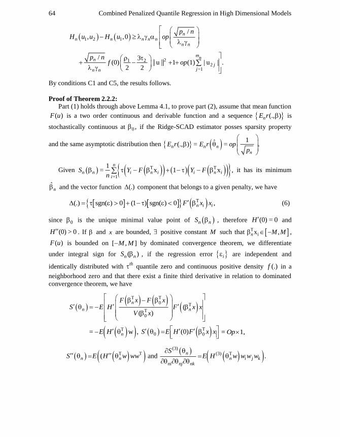
Part (1) holds through above Lemma 4.1, to prove part (2), assume that mean function
( )F u is a two order continuous and derivable function and a sequence (., )nE r is
stochastically continuous at 0 , if the Ridge-SCAD estimator posses sparsity property
and the same asymptotic distribution then 1ˆ(., ) = = .n n n
n
E r E r opp
Given =1
1= x 1 x ,
n
n n i n i i n ii
S Y F Y Fn
it has its minimum
ˆn and the vector function (.) component that belongs to a given penalty, we have
(.) sgn( ) 0 (1 ) sgn( ) 0 ,n i iF x x (6)
since 0 is the unique minimal value point of n nS , therefore (0) = 0H and
(0) > 0H . If and x are bounded, positive constant M such that ix ,n M M ,
( )F u is bounded on [ , ]M M by dominated convergence theorem, we differentiate
under integral sign for ( )n nS , if the regression error i are independent and
identically distributed with th quantile zero and continuous positive density (.)f in a
neighborhood zero and that there exist a finite third derivative in relation to dominated
convergence theorem, we have
0
0
(( )
n
n n
F x F xS E H F x x
V x
= w ,nE H 0 0(0)S E H F x x
= 1,Op
(3)(3)( and .
nn n n i j k
ni nj nk
SS E H w ww E H w w w w

Amin, Song, Thorlie and Wang 65
Some simple calculations show that (0) = 0S and ,11(0) = 2 (0) nS f . By the Taylor
expansion, we have
1ˆ ˆ ˆ ˆ(0) (0) (0)
2
Tn n n nS S S S
(3)
1 1 1
1 ˆ ˆ ˆ .6
k k kn n n
n i j k ni nj nki j k
E H w w w w
(7)
where n is between 0 and ˆ
n . Consider the fourth term of (7) being Z , we show that
1= .PZ o
n
By Caucky-Schwarz inequality and conditions (C2) and (C3), we obtain
2 2
2 (3)
=1 =1 =1 =1 =1 =1
ˆ ˆ ˆw w w wk k k k k kn n n n n n
n i j k ni nj nki j k i j k
Z E H
3 6ˆn nMk
3 3
2
1n nP
k pO
n n
2
1= .Po
n
If V is an identity matrix then, we have
0( )V S
2
0
0
(0)F x
H E xxV x
0 0
0 0
(0) ,F x F x
f E x x
V x V x
where (0) > 0,f we justify that
(.) sgn( ) 0 (1 ) sgn( ) 0n n i iE E F x x
0 sgn( ) 0 (1 ) sgn( ) 0E F x xE
(8)
If the density function of error term is f then (u)f , we have
1
2(u) (0) = Pr (.,u) (.,0) (.) (.,u) (.,0)n n nF F f f n E f f
1 1
2 2 2 21
= | u | | u | u (.) | u |2
n n nn E n S
if n is a sequence of random vectors converging in probability to the value u then
n nF comes within 1Op n then we have 1 (0),n n nOp n F F
1 1
2 2 2 21
= | | | | (.) | |2
n n n n nOp n E Op n

Combined Penalized Quantile Regression in High Dimensional Models 66
Given the empirical process (.) = (.) (.) ,n nE n S S for convenience given that
0
1 10
0
n
n n
F x F x
V x
and 1 10 0
ˆ ˆ ˆ ˆ ˆ ,n n n x x
As per Lemma 4.1, we can conclude that with probability tending to 1,
*ˆ ˆ= .n n n nQ Q Note that Tn i ng Y x , then the linear approximation of ng
near 0 is = (0) (0) ,n n n n ng g E r D where nr is the remainder term.
* * 010 10
=1
ˆ ˆ ˆ( ) (0) = (0) | | | |kn
n n n n n n n nj nj nj j jnj
Q Q S S P
1 ˆ ˆ= (0) (0) (0)n n n nE g g S Sn
010 10
=1
ˆ| | | |kn
n nj nj nj j jnj
P (9)
By considering the third term of (9), using the differential mean value theorem, we get
0
10 10=1
ˆ| | | |kn
nj nj n nj nj j jnj
p
0
1 1
ˆ| | sgnmaxnk
nj n nj i njnj k jn
p
0
1
ˆ| |max nj n nj n njnj k
n
p k
1
2= Po n
If ( )
> 0 as , and nn
n
pn n
then for any that satisfies the
1
20 = ,o n
where i is between 10 j and 10ˆ
nj j , from (7), we have
0
0( ) > 0 (1 ) ( ) < 0 = ( 1) ( ) ( ) ( ) ( ) = 0E sgn sgn f u d u f u d u
hence (.) = (1),nE Op assumes that 1ˆ = ,n n
n
E r Opp
from (9), we have
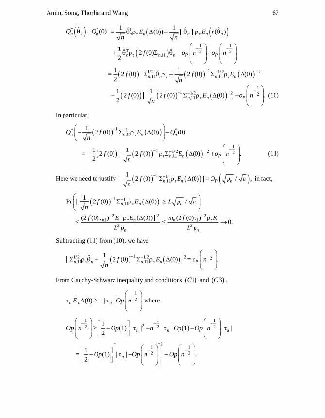
Amin, Song, Thorlie and Wang 67
* *ˆ (0)n n nQ Q 1 1ˆ ˆ ˆ= (0) ( )n n n n nE E rn n
1 1
2 2,11
1 ˆ ˆ2 (0)2
n n n P Pf o n o n
11/2 1/2 2
,11 ,11
1 1ˆ= 2 (0) 2 (0) (0)2
n n n nf f En
1
1 1/2 2 2,11
1 12 (0) 2 (0) (0) .
2n n Pf f E o n
n
(10)
In particular,
1* 1 *
,11
12 (0) (0) (0)n n n nQ f E Q
n
1
1 1/2 2 2,11
1 1= 2 (0) 2 (0) (0) .
2n n Pf f E o n
n
(11)
Here we need to justify 1 1,11
12 (0) (0) = / ,n n P nf E O p n
n
in fact,
1 1,11
1Pr 2 (0) (0) /n n nf E L p n
n
2 21
2
(2 (0) ) ( (0))n n
n
f E E
L p
2
1
2
(2 (0) )0.n
n
m f K
L p
Subtracting (11) from (10), we have
111/2 1/2 2 2
,11 ,11
1ˆ 2 (0) (0) = .n n n n Pf E o nn
From Cauchy-Schwarz inequality and conditions ( 1)C and ( 3)C ,
1
2(0) | |n n nE Op n
where
1 1 1
22 2 21
(1) | | | | (1) | |2
n n nOp n Op n Op Op n
21 1
2 21
= (1) | | ,2
nOp Op n Op n

Combined Penalized Quantile Regression in High Dimensional Models 68
It follows that the square term is at
1
2Op n
and hence
1
2=n Op n
. From
conditions (1) (3)C C , we have,
1/2 1/2,11 1 10
ˆn nn
22
0sgn( ) 0 (1 ) sgn( ) 0E F x xx
2
220sgn( ) 0E F x xx
2
220(1 ) sgn( ) 0E F x xx
2
20 0
( )E F x xx f u du
2
020(1 ) ( )E F x xx f u du
2 2
2 20 01 (0) (1 ) 1 (0)E F x xx F E F x xx F
2 20 0(1 ) (1 ) E F x x F x x
0 0(1 ) ,E F x x F x x
Therefore it is given, 0 0 ,E F x x F x x v
thus (0) belongs to given
penalty, so the condition hold, we obtain
111/2 1/2 1 2
,11 1 10ˆ = (1 )v = (1 ) (0) = (1 ) (0)n nn f f
Hence, we have
21/2 1/2,11 1 10
ˆ 0, (1 ) (0) .D
n nn N f
5. DISCUSSION
In this paper, we study Ridge-SCAD combined penalization technique for variable
selection, coefficient estimation and establish the asymptotic properties of its estimator
when the number of covariates increases to infinity as 0n . Our theory also suggest

Amin, Song, Thorlie and Wang 69
that noncovex combined penalized regression with diverging number of parameters
enjoys oracle property under regularity conditions. Furthermore, we used RCS method to
handle ultrahigh dimensional data. Simulation studies reveal that the performance of
Qr.CP is good when there is high correlations among predictors. The real data analysis
also demonstrated the practical aspects of this method.
REFERENCES
1. Belloni, A. and Chernozhukov, V. (2011). ℓ1-penalized quantile regression in high-
dimensional sparse models. The Annals of Statistics, 39(1), 82-130.
2. Breiman, L. (1996). Heuristics of instability and stabilization in model selection. The
Annals of Statistics, 24(6), 2350-2383.
3. Donoho, D.L. and Johnstone, J.M. (1994). Ideal spatial adaptation by wavelet
shrinkage. Biometrika, 81(3), 425-455.
4. Efron, B., Hastie, T., Johnstone, I. and Tibshirani, R. (2004). Least angle regression.
The Annals of Statistics, 32(2), 407-499.
5. Fan, J. and Li, R. (2001). Variable selection via nonconcave penalized likelihood and
its oracle properties. J. Amer. Statist. Assoc., 96(456), 1348-1360.
6. Fan, J. and Peng, H. (2004). Nonconcave penalized likelihood with a diverging
number of parameters. The Annals of Statistics, 32(3), 928-961.
7. Frank, L.E. and Friedman, J.H. (1993). A statistical view of some chemometrics
regression tools. Technometrics, 35(2), 109-135.
8. Harrison Jr, D. and Rubinfeld, D.L. (1978). Hedonic housing prices and the demand
for clean air. Journal of Environmental Economics and Management, 5(1), 81-102.
9. He, X. and Shao, Q.M. (2000). On parameters of increasing dimensions. Journal of
Multivariate Analysis, 73(1), 120-135.
10. Hoerl, A.E. and Kennard, R.W. (1970). Ridge regression: Biased estimation for non-
orthogonal problems. Technometrics, 12(1), 55-67.
11. Huang, J. and Xie, H. (2007). Asymptotic oracle properties of SCAD-penalized least
squares estimators. Lecture Notes-Monograph Series, 55, 149-166.
12. Huang, J., Horowitz, J.L. and Ma, S. (2008). Asymptotic properties of bridge
estimators in sparse high-dimensional regression models. The Annals of Statistics,
36(2), 587-613.
13. Huber, P.J. (1973). Robust regression: asymptotics, conjectures and Monte Carlo. The
Annals of Statistics, 1, 799-821.
14. Jiang, L., Bondell, H.D. and Wang, H.J. (2014). Interquantile shrinkage and
variable selection in quantile regression. Computational Statistics and Data Analysis,
69, 208-219.
15. Kim, Y., Choi, H. and Oh, H.-S. (2008). Smoothly clipped absolute deviation on high
dimensions. J. Amer.Statist. Assoc., 103(484), 1665-1673.
16. Knight, K. (1998). Limiting distributions for L1 regression estimators under general
conditions. The Annals of Statistics, 26(2), 755-770.
17. Knight, K. and Fu, W. (2000). Asymptotics for lasso-type estimators. Annals of
Statistics, 28(5), 1356-1378.
18. Koenker, R. (2005). Quantile Regression: Cambridge university press.
19. Koenker, R. and Bassett Jr, G. (1978). Regression quantiles. Econometrica: Journal
of the Econometric Society, 46, 33-50.

Combined Penalized Quantile Regression in High Dimensional Models 70
20. Li, G., Peng, H. and Zhu, L. (2011). Nonconcave penalized M-estimation with a
diverging number of parameters. Statistica Sinica, 21(1), 391.
21. Li, G., Peng, H., Zhang, J. and Zhu, L. (2012). Robust rank correlation based
screening. The Annals of Statistics, 40(3), 1846-1877.
22. Ma, S. and Du, P. (2012). Variable selection in partly linear regression model with
diverging dimensions for right censored data. Statistica Sinica, 22(3), 1003-1020.
23. Pollard, D. (1991). Asymptotics for least absolute deviation regression estimators.
Econometric Theory, 7(02), 186-199.
24. Tibshirani, R. (1996). Regression shrinkage and selection via the lasso. J. Roy. Statist.
Soc.. Series B (Methodological), 58(1), 267-288.
25. Wang, L., Wu, Y. and Li, R. (2012). Quantile regression for analyzing heterogeneity
in ultra-high dimension. J. Amer. Statist. Assoc., 107(497), 214-222.
26. Wang, X., Park, T. and Carriere, K. (2010). Variable selection via combined
penalization for high-dimensional data analysis. Computational Statistics and Data
Analysis, 54(10), 2230-2243.
27. Wu, Y. and Liu, Y. (2009). Variable selection in quantile regression. Statistica Sinica,
19(2), 801.
28. Zou, H. and Hastie, T. (2005). Regularization and variable selection via the elastic net.
J. Roy. Statist. Soc.: Series B (Statistical Methodology), 67(2), 301-320.