Fast function-on-scalar regression with penalized basis expansions

Volume 6, Issue 1 2010 Article 28

The International Journal ofBiostatistics

Fast Function-on-Scalar Regression withPenalized Basis Expansions

Philip T. Reiss, New York University and Nathan S. KlineInstitute for Psychiatric ResearchLei Huang, New York University

Maarten Mennes, New York University

Recommended Citation:Reiss, Philip T.; Huang, Lei; and Mennes, Maarten (2010) "Fast Function-on-Scalar Regressionwith Penalized Basis Expansions," The International Journal of Biostatistics: Vol. 6: Iss. 1,Article 28.DOI: 10.2202/1557-4679.1246

UnauthenticatedDownload Date | 6/15/16 2:21 AM

Fast Function-on-Scalar Regression withPenalized Basis ExpansionsPhilip T. Reiss, Lei Huang, and Maarten Mennes

Abstract

Regression models for functional responses and scalar predictors are often fitted by means ofbasis functions, with quadratic roughness penalties applied to avoid overfitting. The fittingapproach described by Ramsay and Silverman in the 1990s amounts to a penalized ordinary leastsquares (P-OLS) estimator of the coefficient functions. We recast this estimator as a generalizedridge regression estimator, and present a penalized generalized least squares (P-GLS) alternative.We describe algorithms by which both estimators can be implemented, with automatic selection ofoptimal smoothing parameters, in a more computationally efficient manner than has heretoforebeen available. We discuss pointwise confidence intervals for the coefficient functions,simultaneous inference by permutation tests, and model selection, including a novel notion ofpointwise model selection. P-OLS and P-GLS are compared in a simulation study. Our methodsare illustrated with an analysis of age effects in a functional magnetic resonance imaging data set,as well as a reanalysis of a now-classic Canadian weather data set. An R package implementingthe methods is publicly available.

KEYWORDS: cross-validation, functional data analysis, functional connectivity, functionallinear model, smoothing parameters, varying-coefficient model

Author Notes: The authors are grateful to the referees for very helpful feedback, to Mike Milham,Eva Petkova, Thad Tarpey and Simon Wood for highly informative discussions, and to GilesHooker for advice on using the R package fda. The first author's research is supported in part byNational Science Foundation grant DMS-0907017.


1 Introduction

A broad array of regression models have been proposed for settings in which theobservations take the form of entire curves or functions. It has become conventionalto distinguish among three basic situations (Ramsay and Silverman, 2005; Chiou etal., 2004):

1. both the responses and the predictors are functions—what might be termedfunction-on-function regression;

2. the responses are scalars and the predictors are functions (scalar-on-functionregression);

3. the responses are functions and the predictors are scalars (function-on-scalarregression).

The terms “functional regression” and “functional linear model” have been appliedto each of these scenarios, so it is important to be clear as to which of the three isunder discussion. This paper describes methodological and computational advancesfor the third scenario, function-on-scalar regression.

Our starting point is the formulation of function-on-scalar regression in Section13.4 of Ramsay and Silverman (2005; hereafter RS), which we begin by brieflyrecapitulating. The basic model is

y(t) = Zβ (t)+ ε(t).(1)

Here the argument t ranges over some finite interval T ⊂R; y(t) is an N-dimensional“vector of functional responses,” i.e., a vector-valued function with values in RN ;Z is an N×q design matrix; β (t) = [β1(t), . . . ,βq(t)]T is the vector of functional ef-fects that we seek to estimate; and ε(t) is a vector of error functions ε1(t), . . . ,εN(t),assumed to be drawn from a stochastic process with expectation zero at each t. Theactual response data may come in one of two forms. We may be given a raw re-sponse matrix

Y =[yi(t j)

]1≤i≤N,1≤ j≤n(2)

derived by sampling the N response curves at points t1, . . . , tn. Alternatively, ifthe outcomes lie in the span of a set of basis functions θ1, . . . ,θK , they can bespecified by an N×K matrix C of basis coefficients such that y(t) =Cθ(t), whereθ(t) = [θ1(t), . . . ,θK(t)]T .

Whether the responses are given in raw form or as basis coefficients, we positthat the coefficient functions β1, . . . ,βq lie in the span of θ1, . . . ,θK . The problem is

1

Reiss et al.: Function-on-Scalar Regression


thereby reduced to estimating B= (b1 . . .bq)T , the q×K matrix of basis coefficients

determining the coefficient functions via

βk(t) = bTk θ(t) for k = 1, . . . ,q.(3)

A key feature of this basis function approach is the use of quadratic roughnesspenalties to avoid overfitting in the estimation of B.

In RS’s formulation, the response and coefficient functions may be expanded intwo different bases. For our purposes, as explained in Appendix A, it suffices toassume the same basis is used for both.

The above framework is probably the most common “entry point” for biostatis-ticians and other data analysts interested in function-on-scalar regression, due tothe relative simplicity and accessibility of the basis function-roughness penalty ap-proach, the status of RS as a foundational text of functional data analysis, and thewide dissemination of associated software for R and Matlab (Ramsay et al., 2009).Still, this basic model does not seem to have been incorporated into many data ana-lysts’ toolkits, in spite of its wide and growing range of potential applications. Weattribute this to several factors:

1. Although the roughness penalty approach is familiar to readers of RS, thefunction-on-scalar regression problem entails somewhat involved matrix al-gebra, so that the route to obtaining the optimal B may seem more opaquethan for other problems solved by roughness penalization.

2. The critical choice of the optimal degree of smoothing requires cross-valida-tion, which is very time-consuming (Ramsay et al., 2009, p. 154). Giventhe need for rapid implementation of modern data analyses, this may renderfunction-on-scalar regression infeasible in many applications.

3. The basis coefficient matrix C of the responses, as opposed to the raw re-sponses Y , is emphasized in RS’s treatment and is assumed in the associatedsoftware (Ramsay et al., 2009), whereas other authors have generally workedwith the raw data.1 This and perhaps other differences in formulation havehindered cross-fertilization between RS’s work and related models, some ofwhich are not explicitly “functional.”2

1This difference is at least partly driven by disparate applications. RS are primarily interested indensely sampled data for which reduction to basis coefficients may be a practical necessity. Relatedwork often deals with longitudinal data that is sparsely and/or irregularly sampled, possibly withsignificant measurement error; here raw responses are more appropriate. The methods of this paperare developed with the former class of applications in mind.

2In particular, RS (p. 259) note that functional-response models are related to varying-coefficientmodels, and suggest that methods developed for the latter may be useful for the former. Indeed,model (1) can be viewed as a repeated-measures varying-coefficient model.

2

The International Journal of Biostatistics, Vol. 6 [2010], Iss. 1, Art. 28

DOI: 10.2202/1557-4679.1246


Our reconsideration of model (1) addresses each of these issues:

1. By a subtle modification of RS’s development, we reduce the objective func-tion to the familiar generalized ridge regression form appearing in the rough-ness penalty approach to nonparametric regression.

2. This reformulation motivates a computational shortcut that enables cross-validation to be performed much faster than with existing software (Sec-tion 8.1 discusses a classic data set for which speed is improved by two ordersof magnitude).

3. We show how our framework casts the RS estimate as a penalized ordinaryleast squares (P-OLS) solution. This motivates a penalized generalized leastsquares (P-GLS) model in basis coefficient space, extending RS’s model andbridging the gap between it and recent work in the varying-coefficient modelliterature.

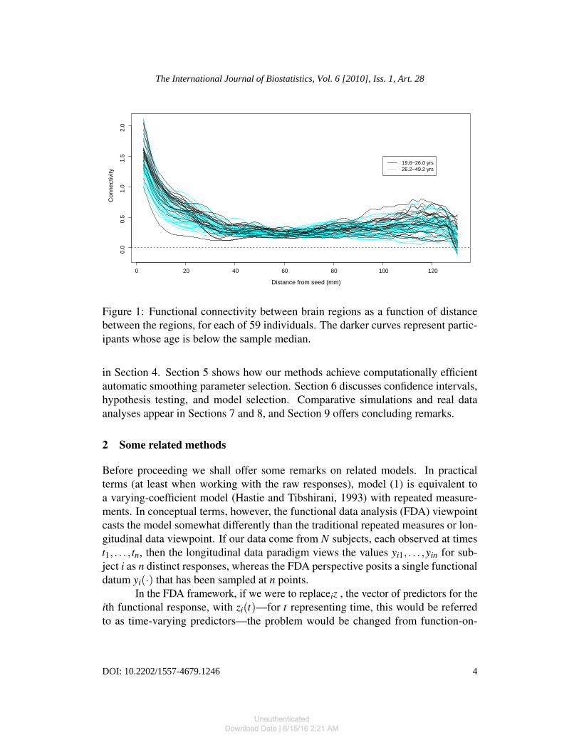
Our work was motivated by a functional magnetic resonance imaging (fMRI)study investigating functional connectivity, or temporal correlation among signalsin different brain locations. By a procedure outlined in Section 8.2, one can ex-press connectivity between locations as a function of the distance between them.Figure 1 displays functions of this kind for each of 59 participants. There is neu-roscientific evidence that the relationship between distance and connectivity mayvary with age, and the figure suggests that there may indeed be systematic differ-ences between the older and younger participants, in particular at short distances.Our application of function-on-scalar regression to model the effect of age on theconnectivity functions will be presented in Section 8.2.

The contributions of this paper can be summarized as follows. First, we de-scribe computationally efficient cross-validation for P-OLS, implemented in thenew refund package for R (R Development Core Team, 2010). Second, we extendRS’s model to P-GLS, with fast automatic selection of multiple smoothing param-eters. Third, we present a generalized ridge regression framework for function-on-scalar regression that encompasses both P-OLS and P-GLS. Fourth, we introducea novel notion of pointwise model selection, which may be more useful than tra-ditional “overall” model selection in many applications. Fifth, we describe twodistinct interval estimation approaches appropriate for P-OLS and for P-GLS re-spectively. Sixth, we compare P-OLS and several variants of P-GLS via simulationsand with reference to the neuroimaging data set mentioned above.

Following some brief remarks on related models in Section 2, we begin ourmain development in Section 3, in which the P-OLS estimator of RS is derived asa generalized ridge estimator. Our P-GLS extension of RS’s model is described

3



0 20 40 60 80 100 120

0.0

0.5

1.0

1.5

2.0

Distance from seed (mm)

Con

nect

ivity

19.6−26.0 yrs26.2−49.2 yrs

Figure 1: Functional connectivity between brain regions as a function of distancebetween the regions, for each of 59 individuals. The darker curves represent partic-ipants whose age is below the sample median.

in Section 4. Section 5 shows how our methods achieve computationally efficientautomatic smoothing parameter selection. Section 6 discusses confidence intervals,hypothesis testing, and model selection. Comparative simulations and real dataanalyses appear in Sections 7 and 8, and Section 9 offers concluding remarks.

2 Some related methods

Before proceeding we shall offer some remarks on related models. In practicalterms (at least when working with the raw responses), model (1) is equivalent toa varying-coefficient model (Hastie and Tibshirani, 1993) with repeated measure-ments. In conceptual terms, however, the functional data analysis (FDA) viewpointcasts the model somewhat differently than the traditional repeated measures or lon-gitudinal data viewpoint. If our data come from N subjects, each observed at timest1, . . . , tn, then the longitudinal data paradigm views the values yi1, . . . ,yin for sub-ject i as n distinct responses, whereas the FDA perspective posits a single functionaldatum yi(·) that has been sampled at n points.

In the FDA framework, if we were to replace zi , the vector of predictors for theith functional response, with zi(t)—for t representing time, this would be referredto as time-varying predictors—the problem would be changed from function-on-

4


DOI: 10.2202/1557-4679.1246


scalar to a form of function-on-function regression, specifically the “concurrent”model treated in Chapter 14 of RS. In this paper we restrict attention to function-on-scalar regression, i.e., non-time-varying predictors, for simplicity.

The most commonly used penalized basis functions for functional data aresplines. The low-rank penalized spline bases favored by RS may be contrasted withtwo alternative spline approaches. On the one hand, roughness penalization allowsfor the use of a rich basis, as opposed to unpenalized spline approaches (Huang etal., 2004) that may require a careful choice of a limited number of knots. On theother hand, low-rank spline bases may offer substantial computational savings oversmoothing splines with a knot at each observation point, even when the latter areefficiently implemented as in Eubank et al. (2004).

A key challenge in function-on-scalar regression is how to contend with de-pendence among the error terms for a given functional response. More explicitly,suppose we are given raw responses (2). Writing the associated stochastic terms as[εi(t j)

]1≤i≤N,1≤ j≤n, we assume that εi1(t j1), εi2(t j2) are independent when i1 6= i2,

but need not be when i1 = i2. One way to address this within-function dependenceis to try to remove it, by incorporating curve-specific effects in the model such thatthe remaining error can be viewed as independent and identically distributed. Indi-vidual curves may be treated as fixed effects (Brumback and Rice, 1998), but havemore often been modeled as random effects (Guo, 2002; Crainiceanu and Ruppert,2004; Bugli and Lambert, 2006). In this paper we are interested in fast computationwith a possibly large number of functional responses, for which estimating individ-ual curves may become infeasible. We therefore focus on the P-OLS and P-GLSmethods, which retain within-function dependence but offer contrasting ways ofdealing with it.

It should also be noted that function-on-scalar regression models can be fittedby approaches other than spline-type basis functions, including kernel and localpolynomial smoothers (e.g., Fan and Zhang, 2000; Chiou et al., 2003, 2004) andwavelets (e.g., Morris and Carroll, 2006; Abramovich and Angelini, 2006; Anto-niadis and Sapatinas, 2007; Ogden and Greene, 2010).

3 The Ramsay-Silverman penalized ordinary least squares estimator

This section revisits RS’s function-on-scalar regression estimator. Our derivationdiffers from that of RS (Section 13.4), and in particular shows how the solution canbe viewed as a generalized ridge regression estimator. This is not merely an exercisein matrix algebra: rather, the ridge regression viewpoint has two key advantages.First, it motivates the enormous computational improvements mentioned above.Second, it casts RS’s estimator as a P-OLS estimator, and points the way toward a

5



P-GLS alternative. We begin with the more conventional raw response form, andthen proceed to the basis coefficient response form; we also derive the latter as alimiting case of the former.

3.1 Responses in raw form: the simplest case

The generalized ridge regression form of the (raw-response) estimator is most trans-parent in the degenerate case in which N = q = 1. Here the raw response ma-trix Y and parameter matrix B reduce to row vectors yT ∈ Rn and bT ∈ RK . Inview of (3), model (1) reduces to the simple nonparametric regression model y =Θb+ ε , where Θ is the basis function evaluation matrix [θ j(ti)]1≤i≤n,1≤ j≤K , andε = [ε(t1), . . . ,ε(tn)]T . (Note that we are temporarily using y and ε to denote vec-tors in Rn, as opposed to the RN-valued functions y(·) and ε(·) defined above.)Taking X = Θ allows us to write this model in the generic form

y = Xb+ ε.(4)

Assuming a rich basis, the least-squares solution b to (4) will yield a function esti-mate β (t) = b

Tθ(t) that is excessively wiggly. Instead we minimize the penalized

sum of squared errors (SSE) criterion

‖y−Xb‖2 +bT Pb,(5)

where P is a positive-semidefinite K×K matrix such that bT Pb provides a measureof the wiggliness of bT

θ(t). This so-called roughness penalty is often given byP = λ

∫[L(bT

θ)(t)]2dt where λ is a nonnegative tuning parameter and L is a lineardifferential operator such as the second derivative operator, for which the aboveintegral equals

∫β ′′(t)2dt. Criterion (5) is minimized by

b = (XT X +P)−1XT y.(6)

We show next that, for general N and q, the RS estimator still has the generalizedridge regression form (6).

3.2 Responses in raw form: the general case

In general the raw responses are modeled as Y = ZBΘT +E,3 where E is the error

matrix [εi(t j)]1≤i≤N,1≤ j≤n. RS (p. 239) propose to estimate B by the minimizer of

3Applications in which it is appropriate to use different bases for the q coefficient functionsrequire a more complex formulation; see Section 14.4 of RS.

6


DOI: 10.2202/1557-4679.1246


the penalized SSE

N

∑i=1

n

∑j=1

[yi(t j)− (ZBΘT )i j]

2 +q

∑k=1

λk

∫[L(bT

k θ)(t)]2dt.(7)

This is the double SSE over the n points at which each of the N functions is sampled,plus roughness penalties on each of the coefficient functions βk(·) = bT

k θ(·), k =1, . . . ,q.

To minimize criterion (7) we require the vec operator and Kronecker products.Recall that vec(M) is the vector formed by concatenating the columns of M, andthat, given the mA× nA matrix A with (i, j) entry ai j, and the mB× nB matrix B,the Kronecker product A⊗B is the (mAmB)× (nAnB) matrix (ai jB)1≤i≤mA,1≤ j≤nA .We can now express the second term of (7) as vec(BT )T (Λ⊗R)vec(BT ), whereΛ= diag(λ1, . . . ,λq) and R is the K×K matrix with (i, j) entry

∫(Lθi)(t)(Lθ j)(t)dt;

and, using the standard identity

vec(ABCT ) = (C⊗A)vec(B),(8)

the first term of (7) equals

‖vec(Y T )−vec[(ZBΘT )T ]‖2 = ‖vec(Y T )− (Z⊗Θ)vec(BT )‖2.

Defining PΛ = Λ⊗R, we can then rewrite criterion (7) in form (5) with outcomevector y = vec(Y T ), design matrix X = Z⊗Θ, penalty matrix P = PΛ, and estimandb = vec(BT ). Thus, for given values of λ1, . . . ,λq, formula (6) leads directly to theestimate (in vector form)

vec(BT) =

[(Z⊗Θ)T (Z⊗Θ)+PΛ

]−1(Z⊗Θ)T vec(Y T ).

Another application of (8), along with other standard Kronecker product results,leads to an alternative expression that may be more convenient (cf. eq. (13.25) ofRS):

vec(BT) =

[(ZT Z)⊗ (ΘT

Θ)+PΛ

]−1(Z⊗Θ)T vec(Y T ).(9)

To provide some intuition about viewing Z⊗Θ as the design matrix, we notethat, whereas ordinary linear regression models the linear dependence of a scalar re-sponse on each predictor, here we are modeling the smooth dependence—capturedby K basis coefficients—of n sampled points of a response function on each pre-dictor. Thus each entry zi j of the “base” design matrix Z gives rise to an n×Ksubmatrix, zi jΘ, of the derived design matrix Z⊗Θ.

It is worth noting that if we replace Θ with In, which may be thought of as adegenerate case of restriction to the span of a basis, then (9) becomes a special caseof the (n-dimensional) multivariate ridge regression estimate of Brown and Zidek(1980).

7



3.3 Responses in basis coefficient form

When the responses are given in the form of an N×K matrix C = (c1 . . .cN)T of

basis coefficients, B is estimated as the minimizer of∫‖Cθ(t)−ZBθ(t)‖2dt +

q

∑k=1

λk

∫[L(bT

k θ)(t)]2dt.(10)

Comparing this with (7), we see that the double SSE has been replaced by theintegral over t of the SSE at point t, i.e. of ∑

Ni=1[c

Ti θ(t)− zT

i Bθ(t)]2.As in the raw response case, we can minimize (10) by formulating it as a gen-

eralized ridge regression criterion. Let Jθθ be the K×K matrix with (i, j) entry∫θi(t)θ j(t)dt. Appendix B shows that criterion (10) can be expressed as

‖vec(J1/2θθ

CT )− (Z⊗ J1/2θθ

)vec(BT )‖2 +vec(BT )T PΛvec(BT ),(11)

which, like (7), has the generalized ridge form (5) with b = vec(BT ) and P = PΛ,but in this case the outcome vector is

y = vec(J1/2θθ

CT ) =

J1/2θθ

c1...

J1/2θθ

cN

(12)

and the design matrix is X = Z⊗ J1/2θθ

. Formula (6) thus yields the estimate

vec(BT) =

[(Z⊗ J1/2

θθ)T (Z⊗ J1/2

θθ)+PΛ

]−1(Z⊗ J1/2

θθ)T vec(J1/2

θθCT ).(13)

One can gain some intuition into this solution by viewing the first (SSE) termof (10), (11) as the SSE for a multivariate linear model with basis coefficients asresponses:4

J1/2θθ

ci = J1/2θθ

BT zi +ui = (zTi ⊗ J1/2

θθ)vec(BT )+ui for i = 1, . . . ,N,(14)

where the error vectors ui = (ui1, . . . ,uiK)T are assumed independent of each other

with common mean zero and covariance matrix Σ.It is instructive to contrast the above design matrix Z ⊗ J1/2

θθwith the raw-

response design matrix Z⊗Θ (see the end of Section 3.2). The submatrices zi jJ1/2θθ

4More precisely, the responses are coefficients with respect to the orthonormal basis given bythe components of the RK-valued function t 7→ J−1/2

θθθ(t). Similarly, outcome vector (12) is the

concatenation of the N response functions’ coefficients with respect to this orthonormal basis.

8


DOI: 10.2202/1557-4679.1246


of the former, like those of the latter, consist of K columns corresponding to the co-efficient functions’ expansion with respect to K basis functions. However, whereasthe latter submatrices have n rows, the former have K—expressing the assumptionthat, even if the functional response data consist of a large number n of points,these contain no more than K “pieces of information” given by K basis coefficients.When Jθθ = IK , (13) reduces again to the multivariate ridge regression estimateof Brown and Zidek (1980), but in this case the multivariate response is the basiscoefficient vector.

In Appendix B we provide further insight into criterion (10) by showing that, inthe orthonormal basis (Jθθ = IK) case, its first term reduces to ‖C−ZB‖2

F , where‖ · ‖F denotes the Frobenius norm—i.e., the sum of squared differences betweencorresponding entries of the N×K matrices C (the observed basis coefficients) andZB (the fitted values of the basis coefficients).

3.4 Relationship between the raw-response and basis coefficient estimators

Estimate (13) can be derived as a limiting case of the raw-response solution givenabove, after a bit of rescaling. To simplify the following, assume T = [0,1]. Ifwe replace the first term of (7) with 1

n ∑Ni=1 ∑

nj=1[yi(t j)− (ZBΘ

T )i j]2, then the raw-

response estimate (9) becomes

vec(BT) =

[(ZT Z)⊗

(1n

ΘT

Θ

)+PΛ

]−1

vec(

1n

ΘTY T Z

).(15)

If we assume a uniform grid of points t j = j/n for j = 1, . . . ,n then, as n→ ∞,1nΘ

TΘ→ Jθθ and 1

nΘTY T →M, where M = [

∫θk(t)yi(t)dt]1≤k≤K,1≤i≤N . We can

alternatively write M = [∫

θk(t)(Pθ yi)(t)dt]1≤k≤K,1≤i≤N , where Pθ is the projectionin L2([0,1]) onto the span of the basis functions θ1, . . . ,θK . It follows that if, fori = 1, . . . ,N, the projection of yi(·) onto this span is given by cT

i θ(·) where ci ∈RK ,then M = JθθCT where C is the N×K matrix with ith row cT

i . Consequently, in thelimit as n→ ∞, (15) becomes

vec(BT) =

[(ZT Z)⊗ Jθθ +PΛ

]−1vec(JθθCT Z),(16)

which is readily shown to equal (13) (cf. RS’s (p. 238) equivalent formula forvec(B)).

The above argument says that, for a given basis, fitting the raw-response modelfor functions sampled on a dense grid is essentially equivalent to projecting theresponses onto the basis and then fitting the basis-coefficient model. In this sense,reducing densely sampled responses to their basis expansion entails no real loss ofinformation.

9



4 Penalized generalized least squares

It is well known that, for a linear model with errors that are not independent andidentically distributed, the best linear unbiased estimate of the coefficient vector isgiven by GLS using the inverse of the error covariance matrix. Two complicationsarise in our setting. First, it is not clear whether the optimality of unpenalized GLSwould carry over to function-on-scalar regression with penalized basis functions(but see Lin et al., 2004, Section 5, for a minimum-variance result that may berelevant). Second, GLS presupposes a known covariance matrix, but in practice thecovariance must be estimated, so that the resulting estimator is technically knownas feasible GLS. For brevity, however, we shall refer to our penalized feasible GLSprocedure as P-GLS.

4.1 Algorithm

The key ingredient of P-GLS is an estimate of the covariance matrix of the outcomesgiven by (12), conditional on the scalar predictors, i.e., the NK×NK covariance ma-

trix of the error vectors

u1...

uN

ˆ ˆ

ˆ

referred to in (14). Under the assumptions given

below (14), the covariance matrix can be written as IN⊗Σ (cf. the “seemingly unre-lated regression” of Zellner, 1962), and the problem reduces to estimating the K×Kmatrix Σ = Cov(ui). This can be done using the N×K matrix U = (u1 . . .uN)

T ofP-OLS residuals given by

vec(UT) = vec(J1/2

θθCT )− (Z⊗ J1/2

θθ)vec(BT

OLS),

ˆ

(17)

where BOLS is the P-OLS estimate (16). Let U∗ denote the matrix formed from Uby centering each column. The covariance can then be estimated by Σ = U∗TU∗/dfor a suitable d. It would be natural to take d = N− d f where d f is the residualdegrees of freedom, but in this context, defining the latter quantity is not straightfor-ward. It therefore seems most reasonable to take d = N, which yields the maximumlikelihood estimate (MLE) under normality.

Given our covariance estimate, the P-GLS criterion is obtained by replacing thefirst (SSE) term of (11) with[vec(J1/2

θθCT )− (Z⊗ J1/2

θθ)vec(BT )

]Tˆ(IN⊗Σ)−1

[vec(J1/2

θθCT )− (Z⊗ J1/2

θθ)vec(BT )

].

(18)

10


DOI: 10.2202/1557-4679.1246


As above, one can use a generalized ridge regression representation to derive theminimizer

vec(BT) =

[(ZT Z)⊗ (J1/2

θθΣ−1

J1/2θθ

)+PΛ

]−1vec(J1/2

θθΣ−1

J1/2θθ

CT Z)(19)

(see Appendix C). Note that this estimate reduces to (16) when Σ = I.As in Krafty et al. (2008), we may wish to estimate B by an iterative P-GLS

procedure:

1. Compute the P-OLS estimate vec(BTOLS) by (16).

2. Use the residuals (17) to obtain a covariance matrix estimate Σ, and insert Σ

into (19) to derive a provisional P-GLS estimate vec(BTGLS).

3. Return to step 2 (now using the P-GLS residuals), and repeat until conver-gence of BGLS.

One goal of the simulations in Section 7 is to evaluate whether iterating to conver-gence improves the performance of P-GLS.

4.2 Other approaches to covariance estimation

The MLE Σ can be inverted only if N >K, and even if this inequality holds, the esti-mate may become unstable for large K. Krafty et al. (2008), in a repeated-measuressetting, assume a covariance matrix of the form Γ+σ2I, where σ2 might be inter-preted as measurement error, and employ a Kullback-Leibler criterion to regularizethe covariance estimate. Their method requires cross-validation over two tuning pa-rameters. This covariance model is especially appropriate when the data are sparseand noisy and when covariance estimation is of intrinsic interest (Yao et al., 2005).In the RS framework, however, the basis coefficients are generally taken to representdenoised functional data, obviating the need for such a computationally intensiveapproach. A less computationally demanding regularized estimate of the covari-ance matrix, using the optimal shrinkage method of Schafer and Strimmer (2005),was tested in simulations (not shown) but did not appear to improve performance.

In the nonparametric regression literature, some authors have used mixed modelsoftware to perform smoothing and estimate correlation structure simultaneously(e.g., Wang, 1998; Durban and Currie, 2003; Krivobokova and Kauermann, 2007).An analogous approach might be attempted for function-on-scalar regression, as analternative to P-GLS. However, this would entail imposing one of several standardparametric correlation structures; and for some examples, such as the periodic func-tional data considered in Section 8.1, none of these structures may be appropriate.

11



5 Smoothness selection

Selection of the smoothing parameters λ1, . . . ,λq is a crucial step,5 and it is here thatour approach attains notable computational efficiency, as this section will explain.

5.1 Leave-one-function-out cross-validation for P-OLS

In the P-OLS setting, the smoothing parameters are usually chosen by a cross-validation (CV) procedure in which one function is left out at a time (Rice andSilverman, 1991). The criterion to be minimized is the cross-validated integratedsquared error

1N

N

∑i=1

∫T[yi(t)− y(−i)

i (t)]2dt,(20)

where y(−i)i (·) is the predicted value for the ith functional response, based on the

model fitted to the other N−1 functional responses. Letting ci and c(−i)i denote the

vectors of basis coefficients determining the two functions in (20), the CV criterion(20) is equal to

1N

N

∑i=1‖J1/2

θθ(ci− c(−i)

i )‖2.(21)

ˆ ˆ

Direct computation of (21) would require fitting the model to almost the entiredata set N times, but this can be avoided by a trick that we shall explain in referenceto the generic penalized regression criterion (5). Suppose the outcome vector ispartitioned into N groups, say y = (yT

1 , . . . ,yTN)

T . Let H be the “hat matrix” suchthat minimizing (5) yields fitted values y = (yT

1 , . . . ,yTN)

T = Hy, and partition Hinto blocks determined by the N groups: H = (Hi j)1≤i≤N,1≤ j≤N . Consider a CVprocedure in which the same model is refitted with each group deleted in turn,and let y(−i)

i denote the fitted values for the ith group based on the group-i-deletedmodel. It can be shown by the Sherman-Morrison-Woodbury formula (e.g., Goluband Van Loan, 1996) that

yi− y(−i)i = (I−Hii)

−1(yi− yi).(22)

If the N groups have one element each, this reduces to yi− y(−i)i = (yi− yi)/(1−

hii) where hii is the ith diagonal element of H. This last identity provides a well-known computational shortcut for ordinary leave-one-out CV. The more general

5Since smoothness is controlled by λ1, . . . ,λq, the precise choice of the number of basis functionsK is generally seen as much less critical, as long as it is large enough to capture the detail of thefunction(s) being estimated. Hence K is often chosen informally (e.g., Ruppert, 2002; Ruppert etal., 2003, pp. 125–127; Wood, 2006a, p. 161).

12


DOI: 10.2202/1557-4679.1246


identity (22) has been used previously for leave-one-function-out CV (Hoover et al.,1998), as well as for multifold CV (Zhang, 1993); our generalized ridge regressionreformulation of RS’s development is what makes it available in the present settingas well. Here the left side of (22) equals J1/2

θθ(ci− c(−i)

i ). Using the results ofSection 3.3 to evaluate the right side of (22), criterion (21) becomes

1N

N

∑i=1

∥∥∥∥∥∥[IK− (zTi ⊗ J1/2

θθ){(ZT Z)⊗ Jθθ +PΛ

}−1(zi⊗ J1/2

θθ)]−1

J1/2θθ

(ci− ci)

∥∥∥∥∥∥2

.

Whereas repeated model fits would require inverting N K(N−1)×K(N−1) matri-ces, the most expensive part of evaluating the above expression is inverting N K×Kmatrices.

We remark that efficiency might be further improved by using k-fold rather thanleave-one-out CV, say with k = 5 or 10. It should also be noted that smoothnessselection for generalized ridge regression is usually accomplished by optimizing notCV but either generalized cross-validation (GCV) or restricted maximum likelihood(REML) (Reiss and Ogden, 2009). However, the latter two criteria presupposethat the error covariance either is a multiple of the identity, or else is taken intoaccount—either by using P-GLS, or by simultaneous estimation of the dependencestructure as mentioned in Section 4.2.

In the single smoothing parameter case, i.e. when λ1 =. . . = λq = λ , the CV cri-terion can be computed rapidly for different values of λ by using Demmler-Reinschorthogonalization (e.g., Ruppert et al., 2003). As an alternative to the usual gridsearch, the generic minimizer implemented in the R function optimize (Brent,1973) appears to work quite well for finding the minimum of the CV score as afunction of λ . Minimizing the CV score as a function of multiple smoothing pa-rameters seems much more difficult, and our current implementation works only forthe common smoothing parameter case. The disadvantages of this restriction maybe overcome to some degree by scaling each predictor to have unit mean square;see also Section 8.2.

5.2 P-GLS

As noted above, the automatic smoothing parameter selection criteria GCV andREML are available for P-GLS. REML appears to be more popular for regressionwith functional responses (e.g., Brumback and Rice, 1998; Guo, 2002; Krafty et al.,2008), and is a particularly natural choice when the model includes random effects.The demonstration by Krivobokova and Kauermann (2007) that REML is morerobust than GCV to misspecification of the correlation structure provides furthersupport for favoring REML in the present setting. In our implementation, smooth-ing parameters are optimized efficiently, within each iteration of the algorithm of

13



ˆ

Section 4.1, by calling the gam function in the mgcv package (Wood, 2006a), towhich a REML option has recently been added (Wood, 2010). This function is, tothe best of our knowledge, the most stable and efficient publicly available softwarefor estimation of separate smoothing parameters λ1, . . . ,λq in models of generalizedridge regression type.

6 Inference

6.1 Pointwise confidence intervals

To derive approximate standard errors for the function estimates βi(t), observe that

βi(t) = θ(t)T BT ei = [eTi ⊗θ(t)T ]vec(BT

)

where ei denotes the vector in Rq with 1 in the ith position and 0 elsewhere, andthus Var[βi(t)] = [eT

i ⊗ θ(t)T ]Var[vec(BT)][ei⊗ θ(t)]. The problem reduces, then,

to estimating the variance of vec(BT). Different approaches to this task have been

proposed for P-OLS and for P-GLS. In either case, however, the variance estimatorcan be explained more clearly by referring to the generic expression (6) with b =

vec(BT).For P-OLS, (6) suggests the variance estimate

Var[vec(BT)] = (XT X +P)−1XT Var(y|X)X(XT X +P)−1

with y, X and P as given in the text immediately preceding (13). As in Section 4.1we can take Var(y|X) = IN ⊗Σ, where Σ is the MLE derived from the residuals in

ˆ

the basis-coefficient domain. Plugging in the values of X and P yields

Var[vec(BT)] = (Z∗TJ Z∗J +PΛ)

−1Z∗TJ (IN⊗Σ)Z∗J(Z∗TJ Z∗J +PΛ)

−1,(23)

where Z∗J = Z⊗ J1/2θθ

.An analogous expression could be derived for P-GLS. Note, however, that this

estimate ignores the added variation due to the need to estimate Λ. In addition,confidence intervals based on (23) may have poor coverage since the roughnesspenalty introduces bias in the estimation of vec(BT ) (Wood, 2006a, 2006b). Thelatter problem can be remedied by instead using Bayesian confidence intervals, orcredible intervals, as developed by Wahba (1983) and Silverman (1985). In Ap-pendix C we obtain the posterior covariance estimate from which such intervals canbe derived:

Var[vec(BT )|Y ] = σ2[(ZT Z)⊗ (J1/2

θθΣ−1

J1/2θθ

)+PΛ

]−1,(24)

14


DOI: 10.2202/1557-4679.1246


where σ2 is a residual variance estimate given there. Appendix C also explains whythis approach works only for P-GLS but not for P-OLS. In summary, then, we baseinterval estimation on the frequentist formula (23) for P-OLS, and on the Bayesianformula (24) for P-GLS.

6.2 Hypothesis testing

RS (p. 227) propose to test the effects of a set of scalar predictors in pointwisefashion by means of F-statistics. Suppose we wish to test a null model with designmatrix Z0 against the alternative model (1). The statistic at point t is given by

F(t) =[‖y(t)−Z0β 0(t)‖2−‖y(t)−Zβ (t)‖2]/(m−m0)

‖y(t)−Zβ (t)‖2/(N−m),

where β 0, β are the function estimates, and m0, m are the model degrees of free-dom, for the null and alternative models respectively. Given the dependence amongmodels at different ts, F(t) may not have the Fm−m0,N−m distribution under the nullmodel. But in any case, inference is not usually performed by referring F(t) ata particular t to an F distribution. More often, one conducts simultaneous test-ing by comparing the observed {F(t) : t ∈ T } to the permutation distribution ofsupt∈T F(t). In practice, one approximates this distribution by Monte Carlo simu-lation. The null model can then be rejected at the 100α% level if, for some t, F(t)exceeds the 100(1−α) percentile of the permuted-data values of supt∈T F(t).

6.3 Overall and pointwise model selection

If permutation tests confirm that each of several scalar predictors has a significanteffect on the functional outcome, it is natural to ask which of these is the most pre-dictive. More generally we may be interested in choosing the best among severalpossibly non-nested function-on-scalar regression models. The P-OLS method of-fers the most straightforward approach to model selection: one can simply selectthe model with the lowest cross-validated integrated squared error (20).

In at least some applications, however, it may make sense to allow for a different“best” model within different subsets of T , the response functions’ domain. It isnatural to perform pointwise model selection criterion for each t ∈ T using thecross-validated pointwise squared error 1

N ∑Ni=1[yi(t)− y(−i)

i (t)]2, i.e. the quantitywhose integral over T equals (20). Note that since the functional linear model“borrows strength” across values of t and thus obtains a smooth estimate of y(−i)

i (·),the proposed pointwise CV criterion should be more stable than naıve ordinaryCV based on fitting the model separately at each t. In practice one would use the

15



equivalent expression 1N ∑

Ni=1[(ci− c(−i)

i )T θ(t)]2, which can be computed withoutrepeated model fits by the methods of Section 5.1.

7 Comparative simulations

We conducted a simulation study using the three-group one-way functional ANOVAmodel6 yi(t) = µ(t)+ βgp(i)(t)+ εi(t) (t ∈ [0,1]), where gp(i) denotes the group(1, 2, or 3) to which the ith functional response belongs. The mean functionµ(t) = 0.4arctan(10x−5)+0.6, and the group effect functions β1(t) =−0.5e−10t

−0.04sin(8t)−0.3t+0.5, β2(t)=−(t−0.5)2−0.15sin(13t), and β3(t)=−β1(t)−β2(t), are shown in the top panels of Figure 2. The error functions εi(·) were sim-ulated from a mean-zero Gaussian process with covariance V (s, t) = σ2

1 0.15|s−t|+σ2

2 δst , where δst = 1 if s = t and = 0 otherwise, sampled at t = m/200 for m =0, . . . ,200 (cf. Section 4.2 above). Note that, although we adopt a fixed-effectsmodeling approach in this paper, for purposes of simulating functional responses itis more natural to think of V (s, t) as arising from a mixed model in which the er-ror is decomposed as εi(t) = εi1(t)+ εi2(t), where Cov[εi1(s),εi1(t)] = σ2

1 0.15|s−t|,Cov[εi2(s),εi2(t)]=σ2

2 δst , and ε11, . . . ,εN1 are independent of ε12, . . . ,εN2. In mixedmodel terms, µ(t)+βgp(i)(t)+εi1(t) is the underlying true function for observationi; σ2

1 represents the variation among the true functions in each group; and σ22 rep-

resents the noise or error variance at each point of these functions, possibly due tomeasurement error. We used samples of Ng = 10,60 for each of the three groups,and two levels of the among-function standard deviation σ1 (0.05 and 0.15); σ2 wasfixed at 0.05. For each combination of Ng and σ1, we simulated 500 data sets, andfitted the model by four methods:

1. P-OLS with a common smoothing parameter λ for all four coefficient func-tions being estimated, chosen by cross-validation;

2. P-GLS with a common λ chosen by REML and with Σ estimated only once,i.e., only one step of the iterative algorithm;

3. same as method 2, but with iteration to convergence;

4. same as method 2, but with separate smoothing parameters λ1–λ4.

The raw responses were smoothed with a 20-knot cubic B-spline basis, by meansof the R function smooth.spline, to produce functions similar to those shown at

6This is not to be confused with the very different type of functional ANOVA studied, for in-stance, by Hooker (2007).

16


DOI: 10.2202/1557-4679.1246


the bottom of Figure 2; model fitting was then performed on the responses in splinecoefficient form. We imposed the constraint β1(t)+β2(t)+β3(t) = 0 at each t bya standard device (Wood, 2006a, pp. 185–186). In simulations not reported here,we tried using GCV rather than REML for the above three versions of P-GLS. Theresults tended to be slightly worse than with REML.

0.0 0.2 0.4 0.6 0.8 1.0

0.2

0.4

0.6

0.8

1.0

Mean function µµ

0.0 0.2 0.4 0.6 0.8 1.0

−0.

4−

0.2

0.0

0.2

0.4

Effect functions ββi

ββ1

ββ2

ββ3

0.0 0.2 0.4 0.6 0.8 1.0

0.0

0.5

1.0

1.5

Responses for σσ1 = 0.05

0.0 0.2 0.4 0.6 0.8 1.0

−0.

50.

00.

51.

01.

5

Responses for σσ1 = 0.15

Figure 2: Top: Mean function µ(·) and group effect functions βi(·) (i = 1,2,3)for the simulations. Bottom: Example smoothed response functions for the threegroups, color-coded as in the top right panel, with σ1 = 0.05 and with σ1 = 0.15.

Figure 3 presents 1000 times the mean integrated squared error in estimatingthe four coefficient functions. The box plots have been truncated to facilitate visualcomparisons; the scale of each subfigure was chosen so as to include at least thelower 95% of each empirical distribution. As one would expect, the error is lowerfor µ than for the group effects βi. Overall, the four methods perform quite simi-larly. The most striking difference is in the easiest scenario (Ng = 60,σ1 = 0.05),in which the three P-GLS methods outperform P-OLS. On the other hand, P-OLSdoes slightly better than P-GLS in the most difficult scenario (Ng = 10,σ1 = 0.15).

Coverage for 95% confidence/credible intervals—in the “across-the-function”sense, i.e., the proportion of the true function lying within the given interval—isshown in Figure 4. The four subfigures use a common scale chosen to include at

17



●

●

●

●

●

●

●

●

●

●

●

●

●

●

●●

●

●

●

●●

●

●

●

●

●

●

●

●

●

●

●

●

●

●

●

●

●

●

●

●

●●

●

●

●●

●

●

●

●

●

●

●

●

●

●●

●

●

●

●

●

●

●

●

●

●●

●

●

●●

●

●

●

●

●●

●

●●

●●

●

●

●

●

●●●

●

●

●

●●

●

●●●

●

●

●

●

●●

●

●

●

●

●

●●

●

●●

●

●

●

●

●

●

●●

●

●

●

●

●●●

●●

●

●

●

●

●

●

●

●

●●

●

●

●●

● ●

●●

●●

●

●

●

●

●

●

●

●

●●

●

●

●●

●

●

●

●

●

●

●

●

●

●

●●●●

●

●

●

●

●●

●

●

●

●

●

●●●

●●

●

●

●

●

●●

●

●

●

●

●

●

●

●●●

●

●

●

●●

●

●

●

●

●●

●

●●●

●

●

●

●●

●

●

●

●●

●

●●

●●

●

●

●

●

●

●

●●

●

●

●

●

●

●

●

●

●●

●

●

●

●

●

●

●

●

●

●

●●

●

●

●

●●

●

●

●

●●

●

●

●

●

●

●

●

●

●

●●

●

●

●

●

●

●

●

●●

●

●●

●

●

●

●

●●●

●●

●

●

●

●

●

●

●

●

●

●

●

●

●

●

●

●

●

●

●●

●

●●

●

●

●

●●

●●

●

●●

●

●

●

●

●●

●

●●

●

●

●

●

●

●

●

●●

●

●

●

●

●

●●

●

●

●

●

10 per group, SD = 0.05

µµ ββ1 ββ2 ββ3

0.0

0.1

0.2

0.3

0.4

0.5

●

●●

●●●●

●

●

●

●

●

●●

●

●

●●●

●

●●●●

●

●●●●

●

●

●

●

●●●●

●

●

●

●●

●

●

●

●

●●

●

●●

●

●

●

●●

●

●

● ●

●●●●

●

●

●

●●

●

●

●

●

●●

●

●●

●

●

●

●

●

●

●

●

●●●●

●

●

●

●

●

●

●

●

●

●●●

●

●

●

●

●

●●

●●

●

●

●

●

●

●

●●

●

●●

●

●

●

●

●

●

●●

●

●

●

●●

●

●

●

● ●

●

●

●

●

●

●

●

●

●

●●

●

●

●

●●

●

●●

●

●

●

●●

●

●

●●

●

●

●

●

●●

●

●●

●

●

●●

●

●

●●

●

●

●

●●●

●

●

●

●

●

●

●

●

●●

●

●●

●

●

●●

●

●

●

●●●

●

●

● ●

●

●

●

●

●

●

●

●

●

●

●

●

●

●

●●

●●

●

●●

●

●

●

●●

●

●

●

●

●

●

●

●●●●●

●

●

●

●

●●

●

●

●

●

●●●

●

●

●

●

●

●

●

●●

●

●

●●

●

●

●●●

●

●

●●●

●

●

●

●

●●

●

●

●

●

●

●

●●

●

●

●

●

●

●

●

●

●

●

●

●

●

●

●

●

●

●

●

●

●

●●

●

●

●●

●

●

●

●

●

●

●

●

●

●

●

●

●

●

●

●

●

●●

●●

●

●

●

●

●

●●

●

●

●

●

●

●●

●

●

●

●

●

●●

●

●

●

●

●

●

●●

●

●

●

●

●

●

●

●

●

●●

●

●

●

●

●●

●

●

●●

●

●

●●

●

●

●

●

●●●

●

●

●

●

●●

●

●

●

●

●

●

●

●

●

●

●

●

●●

●●



01

23

45

●

●

●●

●

●●

●

●

●●

●

●●

●●

●

●●

●

●

●

●

●

●●●

●

●●

●

●

●

●

●●

●

●●

●

●

●●

●

●●

●●

●

●●

●

●

●

●

●

●●●

●

●●

●

●

●

●

●●

●

●●

●

●

●●

●

●●

●●

●

●●

●

●

●

●

●

●●●

●

●●

●

●

●

●

●●

●

●●

●

●●

●●●

●●

●

●●

●

●

●

●

●

●●●

●

●●

●

●

●

●

●

●

●

●

●

●

●

●

●●

●

●

●

●

●

●●

●

●

●

●

●

●

●

●

●

●

●

●

●

●

●

●

●●

●

●

●

●

●

●●

●

●

●

●

●

●

●

●

●

●

●

●

●

●

●

●

●●

●

●

●

●

●

●●

●

●

●

●

●

●

●

●

●

●

●

●

●

●

●●●

●

●

●

●

●●

●

●

●

●

●

●

●

●●

●●

●

●

●

●●●

●

●

●

●

●

●

●

●

●

●

●●

●

●

●

●

●●●

●

●●

●

●●

●●

●

●

●

●

●●●

●

●

●●

●

●

●

●

●

●●

●

●

●

●

●

●●●

●

●

●

●●

●

●

●●

●●

●

●

●

●

●●●

●

●

●●

●

●

●

●

●

●●

●

●

●

●

●

●●●

●

●

●

●●

●

●

●●

●●

●

●

●

●

●●●

●

●

●●

●

●

●

●

●

●●

●

●

●

●

●

●●

●

●

●●

●

●

●

●

●

●

●●

●

●

●

●

●

●●

●

●

●

●

●

●●

●

●

●

●

●

●

●●

●

●

●

●●

●

●

●

●

●

●●

●

●

●

●

●

●●

●

●

●

●

●

●

●●

●

●

●

●●

●

●

●

●

●

●●

●

●

●

●

●

●

●●

●

●

●

●

●

●

●●

●

●

●

●

●

●●

●

●

●

●

●

●

●

●

●

●

●

●

●

●●●

●

●

●

●

●

●



0.00

0.02

0.04

0.06

0.08

●

●

●●

●

●●

●

●

●●

●●

●

●

●●

●

●

●

●

●

●●

●●●

●●●●

●

●

●●

●

●

●●

●

●●

●

●●

●●

●

●

●●

●

●

●

●

●

●●

●●●

●●●●

●

●

●●

●

●

●●

●

●●

●

●●

●●

●

●

●●

●

●

●

●

●

●●

●●●

●●●●

●

●

●●

●

●

●●

●

●

●

●

●●

●●

●

●

●

●●

●

●

●

●

●

●●

●●●

●

●●●

●

●

●

●

●●

●

●

●●

●

●

●

●

●

●

●

●

●

●

●

●

●

●

●

●

●

●

●●

●

●

●

●

●

●

●

●

●

●

●

●●●

●

●●

●

●

●

●

●

●

●

●

●

●

●●

●

●

●

●

●

●●

●

●

●

●

●

●

●

●

●

●

●

●●●

●

●●

●

●

●

●

●

●

●

●

●

●

●●

●

●

●

●

●

●●

●

●

●

●

●

●

●

●

●

●

●

●●●

●

●

●

●

●

●

●

●

●

●

●

●●

●

●

●●

●

●

●

●

●

●

●

●●

●

●

●

●

●

●●

●

●

●●

●

●

●

●

●

●

●●●

●

●

●

●

●

●

●

●

●

●

●

●

●

●

●

●

●

●

●

●

●

●●

●

●

●

●

●

●●

●

●●

●●

●

●

●

●

●

●

●

●

●●

●

●

●

●

●

●●

●

●●

●●

●

●

●

●

●

●

●

●

●●

●

●

●

●●

●●

●

●

●

●

●

●●

●●

●

●

●

●

●

●

●

●●●

●

●

●

●

●

●

●

●

●

●

●

●

●

●

●

●

●

●

●

●

●

●

●

●

●

●

●

●

●

●

●●●

●

●

●

●

●

●

●

●

●

●

●

●

●

●

●

●

●

●

●

●

●

●

●●

●

●

●

●

●

●

●

●

●●●

●

●

●

●

●

●

●

●

●

●

●

●

●

●

●

●

●

●

●

●

●

●

●●

●

●

●

●

●

●

●

●

●

●

●●

●●

●

●

●

●

●

●●

●

●

●

●

●

●

●

●

●

●

●

●

●

●


µµ ββ1 ββ2 ββ30.

00.

20.

40.

60.

8

Figure 3: Mean integrated squared error times 1000, with Ng = 10,60 and withσ1 = .05, .15. Each set of box plots represents the four methods: P-OLS, one-stepP-GLS, iterative P-GLS, and P-GLS with multiple smoothing parameters.

least the upper 95% of each empirical distribution. All methods have median cover-age well above the nominal level, except when Ng = 60,σ1 = 0.05, in which case themedian coverage is quite close to 95%. However, the first quartile of the coverage isseen to lie below 95% in all but one of the box plots. The P-OLS intervals tend to besomewhat wider than their P-GLS counterparts in the Ng = 10,σ1 = 0.15 scenario,and slightly narrower otherwise, especially for Ng = 60,σ1 = 0.05. The lack of aclear overall pattern may arise from two opposing tendencies. On the one hand, thecredible intervals for P-GLS might be wider than the P-OLS confidence intervalsdue to the former’s incorporating a bias correction (see above, Section 6.1); on theother hand, the P-GLS intervals might be too narrow due to not accounting for errorin covariance estimation.

8 Real data examples

8.1 Canadian temperatures

The Canadian weather data set is familiar to students of FDA. RS use this data set toillustrate a number of their methods, and it is included in the fda package (Ramsayet al., 2009). The functional data consist of mean daily temperature and precipita-

18


DOI: 10.2202/1557-4679.1246


●

●

●

●

●

●

●

●●●●●

●

●

●

●

●

●

●

●●

●

●

●

●●

●

●●

●●

●

●

●

●

●

●

●

●

●

●

●●●

●

●

●

●

●

●●●●

●

●

●

●●

●

●

●

●●

●

●

●

●

●

●

●

●

●

●

●

●

●

●

●

●

●

●

●

●

●

●

●

●

●

●

●

●

●●●●●

●

●

●

●

●

●

●

●

●

●

●

●

●

●

●

●

●

●

●

●

●

●

●

●

●

●

●

●

●●

●

●

●

●●●●

●

●●●●●●

●

●

●

●

●

●

●

●

●

●

●

●

●●

●

●

●

●

●

●

●

●

●

●

●

●●

●

●●

●

●

●

●

●

●

●

●

●

●

●

●

●

●

●

●

●

●

●●

●

●

●

●

●

●

●

●

●

●

●●

●

●

●

●

●

●●

●

●

●●

●●●

●

●

●

●

●●

●

●

●

●

●

●

●

●

●

●

●

●

●●

●

●

●

●●

●

●

●

●

●

●

●

●

●

●

●●

●

●

●

●

●

●

●

●

●●●

●

●

●

●●

●

●

●

●

●

●

●

●

●

●●

●

●●

●●

●

●

●●

●

●

●

●

●

●

●

●●

●

●●

●

●

●

●

●

●

●

●

●●●

●

●

●

●

●

●

●

●●●

●

●

●

●

●

●

●

●

●

●

●

●

●●

●

●

●

●

●

●●

●

●

●

●

●

●

●

●

●

●

●

●

●

●●

●

●

● ●

●

●

●

●●●

●

●

●

●

●

●

●●

●

●

●

●

●

●

●

●

●

●

●●

●

●

●●●●

●

●●

●

●●

●

●

●

●●

●

●

●

●

●

●

●

●

●

●

●

● ●

●

●

●

●

●●

●●

●

●

●

●

●●

●

●●

●

●

●

●

●

●

●

●

●

●●

●

●

●

●

●●

●

●●

●

●

●

●

●

●

●

●

●●

●

●

●

●

●

●●

●

●

●

●

●

●

●

●●

●

●

●

●

●

●

●●

●

●

●

●

●●

●

●

●

●

●●●

●

●

●

●

●

●

●

●●●

●

●

●●

●●●

●

●

●●

●

●●

●●

●●

●

●

●

●

●

●

●●

●

●

●

●

●

●

●

●●●

●

●●

●

●

●●●

●●

●

●

●

●

●

●●●●

●

●

●●

●●

●●

●

●

●

●●●

●

●

●

●

●●●

●●

●

●●

●

●●

●

●

●

●

●●●●

●●

●

●

●●

●

●

●

●

●

●

●

●●●●

●

●

●●

●●

●

●

●

●

●

●

●

●

●

●

●

●

●

●●

●

●

●●

●●

●

●

●

●

●●

●

●

●●

●

●

●

●●

●●

●

●

●

●

●

●

●●

●

●

●

●

●

●

●

●

●●●

●

●

●●

●

●

●

●

●●●●



0.4

0.6

0.8

1.0

●

●●●●

●

●

●

●

●

●

●

●

●

●●

●

●

●

●

●●●

●

●

●

●

●

●

●

●

●

●●

●

●●

●●

●

●

●

●

●

●●

●

●

●

●

●

●

●

●

●

●

●

●●●●

●●

●

●

●

●

●

●

●●

●

●

●

●

●

●

●

●

●

●

●

●

●

●

●

●●

●

●

●

●

●

●

●

●

●

●

●

●

●

●●●

●

●

●

●●

●●

●●

●

●

●

●

●

●

●

●

●●

●

●

●

●

●

●

●

●

●

●

●

●

●

●

●

●

●●

●

●

●

●

●

●

●

●

●●

●

●

●

●

●

●●

●

●

●

●

●●

●

●

●

●

●

●

●

●

●

●

●

●

●

●

●

●

●

●

●●

●

●

●

●●

●

●

●

●

●

●

●

●

●

●

●

●

●

●

●

●

●

●

●

●

●

●●

●

●

●●

●

●

●

●

●

●

●●

●

●

●

●

●

●

●

●

●●

●

●●

●

●

●

●

●

●

●●●

●

●

●

●

●

●

●

●

●

●

●

●●

●●●

●●

●

●

●

●

●

●

●

●

●

●

●

●

●

●●

●

●

●

●

●●●

●

●●

●

●●

●

●

●●

●

●

●

●

●●

●

●

●

●

●

●

●

●

●●

●

●

●●●

●

●

●

●

●●●

●●

●

●●

●

●

●

●●

●

●

●

●

●●

●

●

●

●

●

●

●

●●

●●●

●

●

●

●

●

●●

●

●

●

●

●

●

●

●

●

●

●

●

●

●

●

●

●

●

●

●

●

●

●

●

●

●

●

●

●

●

●

●

●

●

●

●

●

●

●

●●●

●

●

●

●

●

●

●●

●

●●

●

●●

●

●●

●●

●

●

●

●

●

●●

●

●

●

●●

●

●

●

●

●

●●

●

●●

●

●

●

●●

●

●

●●

●

●

●

●

●

●

●●

●

●

●●

●●●●

●

●

●

● ●●

●

●

●

●●

●

●

●

●

●

●

●

●

●

●●

●●

●

●

●

●

●

●

●●

●

●

●

●

●●

●●

●

●●

●

●

●

●

●

●

●●

●

●

●

●

●

●

●

●●

●●

●

●

●

●

●

●

●

●

●

●

●●●

●

●

●●

●●●●●

●

●

●

●

●

●●

●

●●●

●

●

●

●

●●●●

●

●

●

●

●

●●

●

●

●

●

●

●

●

●

●

●●

●

●

●

●

●

●

●

●

●●

●●

●

●

●●●

●

●

●

●

●

●

●

●

●

●

●

●

●

●

●

●

●

●

●

●

●

●

●

●

●

●●

●

●●●●

●

●

●

●

●

●

●●

●

●

●

●●

●

●

●

●

●

●

●●

●

●●●●

●●

●

●

●

●

●

●●●●●●



0.4

0.6

0.8

1.0

●

●

●●

●

●

●●

●

●

●

●●

●

●

●

●

●●

●

●●

●

●

●●

●●

●

●●

●

●

●

●

●

●

●

●●

●

●

●

●

●

●

● ●

●●●

●

●

●

●

●

●

●●

●●

●

●

●

●

●

●●●

●

●●

●●

●

●●

●

●

●

●

●

●

●

●●

●

●

●●

●

●

●

●

●●

●●●

●

●

●

●

●

●●

●●

●

●●

●

●

●●●

●

●●

●●

●

●●

●

●

●

●

●

●

●

●●

●

●

●●

●

●

●

●●

●●●

●

●

●

●

●

●

●●

●●●

●●

●

●

●●●

●

●●

●●

●

●●

●

●

●

●

●

●

●

●●

●

●●●●

●

●

●

●

●

●

●

●

●

●

●●●

●

●

●

●

●

●

●

●

●●●●

●

●

●

●●

●

●●●

●●●

●

●

●●●●

●

●

●

●

●

●

●

●●

●

●

●

●

●

●

●●

●●●

●●

●

●

●

●

●●

●

●

●

●●

●

●

●

●

●

●

●

●

●

●

●

●

●

●

●●

●

●●

●

●●

●●

●●

●

●

●●●

●

●

●

●

●

●

●

●

●

●

●

●

●

●

●

●

●

●●

●

●

●

●

●

●●

●

● ●

●

●

●

●●

●

●

●

●

●

●

●

●

●

●

●

●

●

●

●●

●

●●

●

●●

●●

●●

●

●

●●●

●

●

●

●

●

●

●

●

●

●

●

●

●

●

●

●

●

●●●

●

●

●

●●

●

●

●●

●

●

●●

●

●

●

●

●

●

●

●

●

●

●

●

●

●●

●

●●

●

●●

●●●

●

●

●●●

●

●

●

●

●

●

●

●

●

●

●

●

●

●

●

●

●

●

●

●

●

●

●

●

●

●

●●

●

●●●

●

●

●●

●

●

●

●●●

●

●

●

●

●

●

●

●●

●

●

●

●

●

●●

●●

●

●

●

●

●

●

●

●

●●

●

●

●●●

●

●

●

●

●

●

●

●●

●

●

●

●

●

●

●

●●●

●●

●

●

●

●

●

●

●

●

●●

●

●

●●●

●

●

●

●

●

●

●

●●

●

●

●

●

●

●

●

●

●●

●

●

●

●

●

●

●

●

●

●●

●●

●

●●

●

●

●●

●

●

●

●

●●

●

●●

●

●●

●●

●

●

●

●

●

●

●

●

●●●

●

●

●

●

●

●●

●

●

●

●●

●

●

●●●●

●

●

●

●●

●

●

●●

●

●

●

●

●

●

●

●

●

●

●●

●

●

●●●

●

●

●

●

●

●

●●

●

●

●

●●●●

●

●

●

●●

●

●

●●

●

●

●

●

●

●

●

●

●

●

●

●●

●

●

●●●

●

●

●

●●

●

●●

●

●

●

●

●

●

●●

●

●

●

●

●●

●

●

●

●

●

●

●●

●

●

●

●

●

●

●

●

●●

●

●

●●●

●

●

●

●

●●

●

●



0.4

0.6

0.8

1.0

●

●

●

●

●

●

●

●●

●●

●

●

●

●

●

●

●

●

●

●●

●

●

●

●●●

●

●

●

●

●

●

●

●

●

●

●●

●

●

●

●

●

●

●

●

●

●

●

●

●

●

●

●

●

●

●

●●

●

●

●●

●

●

●

●

●

●

●

●

●●●

●

●●

●

●

●

●

●

●

●

●

●

●

●●

●

●

●

●

●●

●

●

●

●

●

●

●

●●

●

●

●

●

●

●

●

●

●

●

●

●

●

●

●

●

●

●

●

●

●

●

●

●●●

●

●

●

●●

●

●

●

●

●

●

●

●

●●●

●

●●

●

●

●

●

●

●

●

●

●

●

●●

●

●

●

●

●

●

●

●

●

●

●

●

●

●

●

●

●

●

●

●

●●

●

●

●

●

●

●

●

●

●

●

●

●

●

●

●

●

●●

●

●

●

●●●

●

●

●

●

●

●

●

●

●

●

●●

●

●

●

●

●

●●

●

●●

●

●

●

●

●●

●

●

●

●

●

●

●●

●

●

●

●

●

●

●●

●

●

●

●

●

●

●

●

●

●

●

●

●

●

●●●

●

●

●●

●

●

●

●

●

● ●

●

●

●

●

●

●

●

●

●

●

●

●

●

●

●

●

●

●

●

●●

●

●

●

●

●

●●

●

●

●

●●

●

●

●●

●

●

●

●

●●

●

●

●

●

●

●

●

●

●

●

●

●

●●

●

●●

●

●

●

●

●

●

●

●

●

●

●

●

●●

●●

●

●

●

●

●

●

●

●

●

●

●

●

●●

●

●

●

●

●

●

●●

●

●

●

●

●

●

●

●

●

●●

●

●

●●

●

●

●

●●

●

●

●●

●

●●●

●●

●

●

●

●

●

●

●

●

●

●

●●

●

●●●●

●

●

●

●

●

●

●

●

●

●

●

●

●●

●

●

●

●

●

●

●●

●

●

●

●

●

●

●

●

●

●●

●

●

●●

●

●

●

●●

●

●

●●

●

●●●

●●

●

●

●

●

●

●

●

●

●

●

●

●

●

●●●

●

●

●

●●

●

●

●

●

●

●

●

●

●●

●

●

●●

●

●

●

●

●

●

●

●

●

●

●

●

●

●

●

●

●

●

●

●

●

●

●

●

●

●

●

●●

●

●

●

●

●

●●

●

●

●

●

●

●

●

●

●

●

●

●●

●

●

●

●

●

●

●

●

●

●●●

●

●

●●●

●

●

●

●

●

●

●●●

●

●●

●

●

●

●

●

●

●

●

●

●

●

●

●

●

●

●●

●

●

●●

●

●

●

●

●

●

●

●

●

●

●

●

●●

●

●

●

●

●

●

●

●

●

●●

●

●

●

●

●

●

●●

●

●●

●

●

●

●

●●

●

●

●

●

●

●

●

●

●●

●

●

●

●

●

●

●

●

●

●

●

●

●

●

●

●

●●

●

●

●

●

●

●●

●●

●

●

●

●

●●

●

●

●

●●

●

●

●

●

●

●

●

●●

●

●

●

●

●

●

●

●●

●

●

●

●

●

●

●

●

●

●●

●

●

●

●

●

●

●

●

●

●

●

●

●

●

●

●

●●

●

●

●

●

●

●

●

●

●

●

●

●

●

●

●

●

●

●●

●

●

●

●

●

●

●

●●

●

●

●

●

●●

●

●

●

●

●

●

●

●

●●

●

●

●

●

●

●

●

●

●

●

●

●

●

●●

●

●

●

●

●

●

●

●

●

●

●

●

●

● ●

●

●

●

●

●

●

●

●

●

●

●

●

●

●

●

●

●

●

●

●●

●

●

●

●

●

●

●●

●

●●

●

●

●

●●

●

●

●

●

●

●

●

●

●●

●

●●●

●

●

●

●

●

●

●

●●

●●●

●

●●●●

●

●

●

●

●

●●

●●

●

●

●

●

●

●

●

●

●●

●

●

●

●

●

●

●

●●●

●

●

●●●●●

●

●

●

●

●

●

●

●

●

●

●

●

●

●

●

●

●●

●

●●●

●

●

●

●

●

●

●

●

●

●●●

●

●●●

●●

●

●

●

●

●

●●

●●

●

●●

●

●

●

●

●

●●

●

●

●

●

●

●

●

●●●

●

●

●

●●●●●

●

●

●

●

●

●

●

●

●

●

●

●

●

●

●

●

●●

●

●●●

●

●

●

●

●

●

●

●

●

●●●

●

●

●

●

●

●

●

●

●

●

●●

●●

●

●

●

●

●

●

●

●

●●

●

●

●

●

●

●

●

●●●

●

●

●●●●●

●

●

●

●

●

●

●

●

●

●

●

●

●

●

●

●

●●●●●

●

●

●

●

●

●

●

●●

●●●

●

●



0.4

0.6

0.8

1.0

Figure 4: Observed across-the-function coverage for 95% confidence/credible in-tervals. Each set of box plots represents the four methods: P-OLS, one-step P-GLS,iterative P-GLS, and P-GLS with multiple smoothing parameters.

tion for the years 1960–1994 at 35 stations across Canada. Here we consider P-OLSregression of the temperature curves on two scalar variables: the region in whichthe station is located (Arctic, Atlantic, Continental, or Pacific), and the station’slatitude. Projecting the temperature functions onto the Fourier basis consisting ofa constant function along with fk(t) = sin(2πkt/365) and gk(t) = cos(2πkt/365)for k = 1, . . . ,12 yields the curves shown at left in Figure 5. Tests of the two pre-dictors based on 300 permutations, as described in Section 6.2, found both to beextremely significant: indeed, in both cases, the real-data F statistic at each pointlay far into the right tail of the simulated permutation distribution of maximal Fstatistics. These results come as no great surprise. A more interesting question con-cerns the two predictors’ comparative strength. Which tells us more about a site’saverage temperature: knowing which region it belongs to, or knowing its latitude?This question can be answered separately for each day of the year by the pointwiseCV method of Section 6.3. As Figure 5 shows, for the period from May throughNovember, latitude has lower CV, and thus appears to be a stronger determinant oftemperature. From January through April, however, regional differences—such as,perhaps, the tendency for coastal areas to have milder winters—appear to be moreimportant than latitude alone.

19



Mea

n te

mpe

ratu

re

Jan Feb Mar Apr May Jun Jul Aug Sep Oct Nov Dec

−30

−20

−10

0

10

20

MS

E.C

V

RegionLatitude

1020

3040

Jan Feb Mar Apr May Jun Jul Aug Sep Oct Nov Dec

Figure 5: At left, smoothed curves representing daily mean temperatures at the 35Canadian locations. At right, pointwise cross-validation MSE for regression of thetemperature functions on region (solid curve) and on latitude (dashed curve).

a 2.16 GHz Intel Core Duo processor, required 2.9 seconds to optimize λ by cross-validation over a grid of 21 candidate values (or 5.1 seconds to find λ via theoptimize function with the default tolerance level, which gives higher accuracythan would usually be needed). By contrast, the function fRegress.CV in the fda

package, which refits the model for each delete-one-function data set, needed about32 seconds to compute the CV for a single candidate λ . Thus, calling fRegress.CVfor each λ in the same grid of values would take over 200 times as long as ourmethod.

8.2 Functional connectivity

We now return to the fMRI data displayed in Figure 1. In traditional fMRI exper-iments, the blood oxygen level dependent (BOLD) signal, an index of brain activ-ity, is recorded at each of a dense grid of brain locations, known as voxels, whilethe subject attends to a series of stimuli. By contrast, our data were acquired byresting-state fMRI, in which subjects are scanned while they attend to no stimulusin particular. The objective is not to study the brain’s response to particular stimuli,but to investigate functional networks of brain regions whose BOLD time coursesmove in tandem. A popular analytic strategy involves choosing a “seed” brain re-gion, and computing the correlation between its BOLD time series and those of

Our P-OLS implementation, running in R version 2.9.0 on a MacBook Pro with

20


DOI: 10.2202/1557-4679.1246


every voxel in the brain. A recent set of seed correlation analyses (Kelly et al.,2009) suggests that as the brain develops from childhood to adulthood, high corre-lations between distant brain regions become more prevalent. As a tool for studyingthe relationship between connectivity and distance from a given seed, we have de-veloped subject-specific connectivity-distance functions. Briefly, these functionsare derived by applying the inverse hyperbolic tangent (or Fisher z transform) tothe correlations of each voxel with the seed region, then estimating a conditionalquantile (say, the 95th percentile) of the resulting values as a smooth function ofdistance from the seed (Koenker et al., 1994). The fitted function is then projectedonto a cubic B-spline basis with 40 equally-spaced internal knots. Repeating thisfor each of N subjects yields functional responses y1(·), . . . ,yN(·), which we mod-eled as yi(d) = β1(d)+ziβ2(d)+εi(d), where d denotes distance from the seed andzi is the ith subject’s age.

This model was fitted to data from 59 participants, ranging in age from 20 to49, who were scanned at New York University. Distance was measured from aseed located in the posterior cingulate/precuneus region, and age was centered tomean zero. The first plot in Figure 6 shows an estimate of β1; this function ishighest for short distances, as expected, but it also has a slight peak around 120mm. The next two plots display estimates of β2 from P-GLS and P-OLS models,respectively, with a common smoothing parameter λ used for both β1 and β2. Theseestimates resemble each other closely but seem rather too bumpy, evidently because|β1(d)| � |β2(d)| for most d, so that the penalty λ

∫β ′′21 +λ

∫β ′′22 is dominated by

its first term. A P-GLS fit with separate smoothing parameters for β1 and β2 yieldsa much smoother estimate of the latter, as seen in the lower left plot.

Although our P-OLS implementation assumes a common λ , multiple smoothingparameter selection can be achieved, in effect, by rescaling. Consider fitting themodel yi(d) = β1(d)+ z∗i β ∗2 (d)+ εi(d), where z∗i = czi and β ∗2 (d) = β2(d)/c forsome c > 0, with a common λ , thereby obtaining the estimate β ∗2 , and taking cβ ∗2as the estimate for β2. This is practically equivalent to fitting the original model withseparate parameters λ1,λ2 related by λ1 = c2λ2. We can thus fit rescaled modelswith a range of values of c = λ1/λ2, and choose the CV-minimizing c. (For

√a model having more than one scalar predictor, CV would have to be minimizedover a multidimensional grid.) The optimal value c = .00056 yielded the age effectfunction shown in the lower center plot of Figure 6. This is quite similar to the P-GLS estimate with separate smoothing parameters, but the 95% confidence intervalis wider. The lower right plot shows expected profiles at the first and third quartilesof the age distribution. All four model fits point to a negative age effect at shortdistance from the seed, and little or no effect at longer distances. A simultaneoustest based on 1500 permutations (not shown) found a significant (at the 5% level)

21



negative effect of age, for distances up to 24 mm from the seed. Our observationthat older subjects’ high-connectivity regions tend to be less concentrated aroundthe seed is consistent with the findings of Kelly et al. (2009).

0 20 40 60 80 100 120

0.2

0.6

1.0

1.4

Mean connectivity−distance profile


Coe

ffici

ent f

unct

ion

0 20 40 60 80 100 120

−0.

020

−0.

010

0.00

0

P−GLS with single smoothing parameter

Distance from seed (mm)C

oeffi

cien

t fun

ctio

n0 20 40 60 80 100 120

−0.

020

−0.

010

0.00

0

P−OLS with single smoothing parameter


Coe

ffici

ent f

unct

ion

0 20 40 60 80 100 120

−0.

020

−0.

010

0.00

0

P−GLS with multiple smoothing parameters


Coe

ffici

ent f

unct

ion

0 20 40 60 80 100 120

−0.

020

−0.

010

0.00

0

P−OLS with age rescaled


Coe

ffici

ent f

unct

ion

0 20 40 60 80 100 120

0.2

0.6

1.0

1.4

Expected profiles at 1st and 3rd quartiles of age


Exp

ecte

d va

lue

23.3 yrs33.1 yrs

Figure 6: The upper left plot shows the estimate (solid) and 95% credible inter-val (dashed) for the intercept function β1 in the fMRI application. The next fourplots show the estimates and 95% intervals for the age effect function β2, derivedby P-GLS and P-OLS with a single smoothing parameter; P-GLS with multiplesmoothing parameters; and P-OLS with a single smoothing parameter, but withage optimally rescaled. The lower right plot shows expected profiles at the firstand third quartiles (solid and dashed, respectively) of the observed age distribution.The upper left and lower right plots are based on the P-GLS model with multiplesmoothing parameters, but the other models produced similar results.

9 Conclusion

It is difficult to choose a clear “winner” between the two basic methods we havediscussed. P-OLS is more conceptually straightforward and less vulnerable to un-dercoverage in small samples; moreover, the CV score, computed in the course ofsmoothing parameter selection, can double as a criterion for selecting among dif-ferent models, in either an overall or a pointwise sense. On the other hand, ourimplementation of P-GLS with the mgcv package allows for rapid selection of mul-tiple smoothing parameters, the advantages of which are apparent from our analysisof the connectivity data. Our simulation results do not unequivocally favor eitherP-OLS or any version of P-GLS, although they suggest that P-GLS may becomemore accurate for functional ANOVA with relatively large, homogeneous groups

22


DOI: 10.2202/1557-4679.1246


of functional responses. The relative merits of P-OLS and P-GLS should becomeclearer as these methods are applied to a wider variety of data sets. It is our hopethat our fast implementation of function-on-scalar regression will contribute to themore widespread application of models of this type.

As noted above (see footnote 1 and Section 4.2), in this paper we have beenprimarily concerned with densely sampled functional data of the type emphasizedby RS. Rather different approaches have been developed for sparsely and irregularlysampled data with significant measurement error (e.g., Chiou et al., 2003, 2004; Yaoet al., 2005; Krafty et al., 2008). It would be of great interest to demarcate moreprecisely the types of applications for which each approach is best suited.

A number of extensions of our methods are planned, including smooth (as op-posed to linear) dependence of the functional response on continuous scalar pre-dictors; generalized linear models with functional responses; and permutation testsappropriate for more complex designs. The methods described here are imple-mented in the R package refund (regression with functional data), available athttp://cran.r-project.org/web/packages/refund.

Appendix A: Reduction to using the same bases for the responses and coefficientfunctions

The first term of equation (10) gave the (unpenalized) integrated SSE as∫‖Cθ(t)−

ZBθ(t)‖2dt. In RS’s (Section 13.4) formulation, the functional responses are givenby y(t) =Cφ(t), where φ(t) = [φ1(t), . . . ,φKy]

T for some basis functions φ1, . . . ,φKy

not necessarily coinciding with the basis functions θ1, . . . ,θK used to expand thecoefficient functions. We show here why, for our purposes, it suffices to assumethat the bases do coincide.

The integrated SSE can be written as

∫‖Cφ(t)−ZBθ(t)‖2dt =

N

∑i=1

∫[cT

i φ(t)− zTi Bθ(t)]2dt,(25)

i.e., this criterion can be expressed either as an integral of a SSE, or as a sum ofintegrated squared errors. Let c∗Ti θ be the orthogonal projection (in L2) of cT

i φ

onto the span of θ1, . . . ,θK; it is easily shown that c∗i = J−1θθ

Jθφ ci, where whereJθφ is the K×Ky matrix with (i, j) entry

∫θi(t)φ j(t)dt. By the definition of an

orthogonal projection, we have the orthogonal decomposition

cTi φ − zT

i Bθ = (cTi φ − c∗Ti θ)+(c∗Ti θ − zT

i Bθ),

23



right side of (25) can be decomposed as∫[cT

i φ(t)− c∗Ti θ(t)]2dt +∫[c∗Ti θ(t)− zT

i Bθ(t)]2dt.

The first of these two integrals does not depend on B. Consequently, the problemof finding B to minimize the penalized SSE (i.e., (25) plus a roughness penalty) isunchanged if we replace Cφ(t) with C∗θ(t), where C∗ = (c∗1 . . .c

∗N)

T = CJTθφ

J−1θθ

.For our development, then, we can assume that {φ1, . . . ,φKy}= {θ1, . . . ,θK}.

Appendix B: Derivation of alternative expressions for criterion (10)

Here we derive expression (11), and a further simplification in the orthonormalbasis case. We have∫

‖Cθ(t)−ZBθ(t)‖2dt =∫

tr[(C−ZB)T (C−ZB)θ(t)θ(t)T ]dt

= tr[(C−ZB)T (C−ZB)Jθθ ]

= tr[{(C−ZB)J1/2θθ}T{(C−ZB)J1/2

θθ}]

= ‖vec(J1/2θθ

CT − J1/2θθ

BT ZT )‖2(26)

= ‖CJ1/2θθ−ZBJ1/2

θθ‖2

F .(27)

By (8), (26) equals the first term of (11). The second (penalty) term of (11) is thesame as in the raw response case (Section 3.2). We therefore conclude that (10)equals (11), as claimed in Section 3.3. In the orthonormal case we take J1/2

θθ= IK

in (27), and immediately obtain the simpler expression ‖C−ZB‖2F .

Appendix C: Derivation of the P-GLS estimate and posterior covariance ma-trix

The Cholesky decomposition Σ−1

= LT L allows us to write the P-GLS criterion,i.e., the SSE (18) plus the second (penalty) term of (11), as∥∥∥∥vec(LJ1/2

θθCT )− [Z⊗ (LJ1/2

θθ)]vec(BT )

∥∥∥∥2+vec(BT )T PΛvec(BT ).(28)

This criterion can be thought of as arising from “prewhitening” each observation viapremultiplication by L, and then performing P-OLS. Expression (28) has form (5)with X = Z⊗ (LJ1/2

θθ), y = vec(LJ1/2

θθCT ), and (as above) b = vec(BT ) and P = PΛ,

and thus, by the Pythagorean identity for inner product spaces, the integral on the

24


DOI: 10.2202/1557-4679.1246


so that (6) gives the minimizer

vec(BT) =

[{Z⊗ (LJ1/2

θθ)}T{Z⊗ (LJ1/2

θθ)}+PΛ

]−1

×[Z⊗ (LJ1/2θθ

)]T vec(LJ1/2θθ

CT ),

which is easily shown to equal (19).For posterior covariance estimation, the key result (Wood, 2006a, pp. 190–191;

Wood, 2006b, p. 450) is that if (4) holds with ε ∼ N(0,σ2I) and b is given by (6),then b has posterior distribution

b|y∼ N[b,σ2(XT X +P)−1].

Given a reasonably accurate estimate of Σ, these assumptions hold approximatelywith X , y, b, P as above, leading to the estimate

Var[vec(BT )|Y ] = σ2[{Z⊗ (LJ1/2

θθ)}T{Z⊗ (LJ1/2

θθ)}+PΛ

]−1,(29)

for a residual variance estimate σ2. Given the hat matrix H such that y≡ Xb = Hy,we can use the standard estimate σ2 = ‖y− y‖2/[NK− tr(H)] (e.g., Wood, 2006a).A bit of algebra reduces (29) to (24).

It is important to note that since the residual error variance cannot be taken asσ2I without prewhitening the data, the above derivation is not valid for P-OLS.

References

Antoniadis, A., and Sapatinas, T. (2007). Estimation and inference in functionalmixed-effects models. Computational Statistics and Data Analysis 51, 4793–4813.

Brent, R. (1973). Algorithms for Minimization Without Derivatives. EnglewoodCliffs, NJ: Prentice-Hall.

Brown, P. J., and Zidek, J. V. (1980). Adaptive multivariate ridge regression. Annalsof Statistics 8, 64–74.

Brumback, B. A., and Rice, J. A. (1998). Smoothing spline models for the analysisof nested and crossed samples of curves. Journal of the American StatisticalAssociation 93, 961–976.

Bugli, C., and Lambert, P. (2006). Functional ANOVA with random functionaleffects: an application to event-related potentials modelling for electroen-cephalograms analysis. Statistics in Medicine 25, 3718–3739.

25



¨

¨

˜

Chiou, J. M., Muller, H. G., and Wang, J. L. (2003). Functional quasi-likelihoodregression models with smooth random effects. Journal of the Royal StatisticalSociety, Series B 65, 405–423.

Chiou, J. M., Muller, H. G., and Wang, J. L. (2004). Functional response models.Statistica Sinica 14, 675–693.

Crainiceanu, C. M., and Ruppert, D. (2004). Restricted likelihood ratio tests innonparametric longitudinal models. Statistica Sinica 14, 713–729.

Durban, M., and Currie, I. D. (2003). A note on P-spline additive models withcorrelated errors. Computational Statistics 18, 251–262.

Eubank, R. L., Huang, C., Munoz-Maldonado, Y., Wang, N., Wang, S., andBuchanan, R. J. (2004). Smoothing spline estimation in varying-coefficientmodels. Journal of the Royal Statistical Society, Series B 66, 653–667.

Fan, J., and Zhang, J.-T. (2000). Two-step estimation of functional linear modelswith applications to longitudinal data. Journal of the Royal Statistical Society,Series B 62, 303–322.

Golub, G. H., and Van Loan, C. F. (1996). Matrix Computations, 3rd ed. Baltimore:Johns Hopkins University Press.

Guo, W. (2002). Functional mixed effects models. Biometrics 58, 121–128.Hooker, G. (2007). Generalized functional ANOVA diagnostics for high-

dimensional functions of dependent variables. Journal of Computational andGraphical Statistics 16, 709–732.

Hoover, D. R., Rice, J. A., Wu, C. O., and Yang, L. P. (1998). Nonparametricsmoothing estimates of time-varying coefficient models with longitudinal data.Biometrika 85, 809–822.

Huang, J. Z., Wu, C. O., and Zhou, L. (2004). Polynomial spline estimation and in-ference for varying coefficient models with longitudinal data. Statistica Sinica14, 763–788.

Kelly, A. M. C., Di Martino, A., Uddin, L. Q., Shehzad, Z., Gee, D. G., Reiss, P.T., Margulies, D. S., Castellanos, F. X., and Milham, M. P. (2009). Develop-ment of anterior cingulate functional connectivity from late childhood to earlyadulthood. Cerebral Cortex 19, 640–657.

Koenker, R., Ng, P., and Portnoy, S. (1994). Quantile smoothing splines. Biometrika81, 673–680.

Krafty, R. T., Gimotty, P. A., Holtz, D., Coukos, G., and Guo, W. (2008). Vary-ing coefficient model with unknown within-subject covariance for analysis oftumor growth curves. Biometrics 64, 1023–1031.

26


DOI: 10.2202/1557-4679.1246


Krivobokova, T., and Kauermann, G. (2007). A note on penalized spline smoothingwith correlated errors. Journal of the American Statistical Association 102,1328–1337.

Lin, X., Wang, N., Welsh, A. H., and Carroll, R. J. (2004). Equivalent kernels ofsmoothing splines in nonparametric regression for clustered/longitudinal data.Biometrika 91, 177–193.

Morris, J. S., and Carroll, R. J. (2006). Wavelet-based functional mixed models.Journal of the Royal Statistical Society, Series B 68, 179–199.

Ogden, R. T., and Greene, E. (2010). Wavelet modeling of functional random ef-fects with application to human vision data. Journal of Statistical Planningand Inference 140, 3797–3808.

R Development Core Team (2010). R: A language and environment for statisticalcomputing. R Foundation for Statistical Computing, Vienna, Austria. ISBN3-900051-07-0, URL http://www.R-project.org.

Ramsay, J. O., Hooker, G., and Graves, S. (2009). Functional Data Analysis with Rand MATLAB. New York: Springer.

Ramsay, J. O., and Silverman, B. W. (2005). Functional Data Analysis, 2nd ed.New York: Springer.

Reiss, P. T., and Ogden, R. T. (2009). Smoothing parameter selection for a class ofsemiparametric linear models. Journal of the Royal Statistical Society, SeriesB 71, 505–523.

Rice, J. A., and Silverman, B. W. (1991). Estimating the mean and covariance struc-ture nonparametrically when the data are curves. Journal of the Royal Statisti-cal Society, Series B 53, 233–243.

Ruppert, D. (2002). Selecting the number of knots for penalized splines. Journal ofComputational and Graphical Statistics 11, 735–757.

Ruppert, D., Wand, M. P., and Carroll, R. J. (2003). Semiparametric Regression.Cambridge and New York: Cambridge University Press.

Schafer, J., and Strimmer, K. (2005). A shrinkage approach to large-scale covari-ance matrix estimation and implications for functional genomics. StatisticalApplications in Genetics and Molecular Biology 4, article 32.

Wahba, G. (1983). Bayesian “confidence intervals” for the cross-validated smooth-ing spline. Journal of the Royal Statistical Society, Series B 45, 133–150.

Wang, Y. (1998). Smoothing spline models with correlated random errors. Journalof the American Statistical Association 93, 341–348.

Wood, S. N. (2006a). Generalized Additive Models: An Introduction with R. BocaRaton, FL: Chapman & Hall.

27



¨

Wood, S. N. (2006b). On confidence intervals for generalized additive models basedon penalized regression splines. Australian and New Zealand Journal of Statis-tics 48, 445–464.

Wood, S. N. (2010) Fast stable REML estimation of semiparametric GLMs. Journalof the Royal Statistical Society, Series B, to appear.

Yao, F., Muller, H.-G., and Wang, J.-L. (2005). Functional data analysis for sparselongitudinal data. Journal of the American Statistical Association 100, 577–591.

Zellner, A. (1962). An efficient method of estimating seemingly unrelated regres-sions and tests for aggregation bias. Journal of the American Statistical Asso-ciation 57, 348–368.

Zhang, P. (1993). Model selection via multifold cross validation. Annals of Statistics21, 299–313.

28


DOI: 10.2202/1557-4679.1246


Fast function-on-scalar regression with penalized basis expansions

Documents

Transcript of Fast function-on-scalar regression with penalized basis expansions