Cornell University ILR SchoolDigitalCommons@ILR

Articles & Chapters ILR Collection

7-29-2008

CEO Pay-For-Performance Heterogeneity:Examples Using Quantile RegressionKevin F. HallockCornell University, kfh7@cornell.edu

Regina MadalozzoIbmec Sao Paulo

Clayton G. ReckCRA International

This Article is brought to you for free and open access by the ILR Collection at DigitalCommons@ILR. It has been accepted for inclusion in Articles &Chapters by an authorized administrator of DigitalCommons@ILR. For more information, please contact jdd10@cornell.edu.

Please take our short DigitalCommons@ILR user survey.

Hallock, Kevin F.; Madalozzo, Regina; and Reck, Clayton G., "CEO Pay-For-Performance Heterogeneity: Examples Using QuantileRegression" (2008). Articles & Chapters. Paper 198.http://digitalcommons.ilr.cornell.edu/articles/198

CEO PAY-FOR-PERFORMANCE HETEROGENEITY USING QUANTILE REGRESSION

Kevin F. Hallock*

Cornell University and NBER

Regina Madalozzo Ibmec Sao Paulo

Clayton G. Reck CRA International

July 29, 2008

ABSTRACT

We provide some examples of how quantile regression can be used to investigate heterogeneity in pay–firm size and pay-performance relationships for U.S. CEOs. For example, do conditionally (predicted) high-wage managers have a stronger relationship between pay and performance than conditionally low-wage managers? Our results using data over a decade show, for some standard specifications, there is considerable heterogeneity in the returns to firm performance across the conditional distribution of wages. Quantile regression adds substantially to our understanding of the pay-performance relationship. This heterogeneity is masked when using more standard empirical techniques.

JEL: M52, J33, G3 Keywords: Executive compensation, quantile regression, pay and performance

© 2008 Kevin F. Hallock, Regina Madalozzo and Clayton G. Reck.

* Corresponding author Kevin F. Hallock, Departments of Labor Economics and HR Studies, 391 Ives Hall, Cornell University, Ithaca, NY 14853, 607.255.3193, 607.255.1836 (fax), hallock@cornell.edu.

George Baker, David Balan, Martin Conyon, John Core, Brian Hall, Kevin Murphy, Paul Oyer, Scott Schaefer, and seminar participants at the American Economic Association meetings provided very helpful suggestions. We are especially grateful to Roger Koenker for numerous conversations on the topic of quantile regression and to Scott Schaefer for carefully commenting on a very preliminary version.

1. Introduction

This paper uses quantile regression as introduced in Koenker and Bassett (1978) to

investigate heterogeneity in the relationship between CEO pay and firm performance. There

have been hundreds of papers published on executive compensation in the past 20 years in

economics, finance, human resource management, and accounting. A great deal of these have

focused on the relationship between the compensation of the top manager and the size of the

firm or between the compensation of the top manager and the performance of the firm. Most,

however, have focused on the estimated mean relationship. This paper will use some examples

to show that the mean returns mask substantial heterogeneity in the CEO pay and firm

performance relationship.

Murphy’s (1985) work helped start a surge of interest in this area. Jensen and Murphy

(1990) found that CEO wealth changes were only weakly related to firm value changes, and the

link was probably too low to provide meaningful management incentives. Hall and Liebman

(1998) showed that since stock options are such an important part of managerial pay, the value

of options are obviously related to firm value, and there is a link between managerial pay and

firm performance.

Most of the important research on the pay versus firm performance relationship has

been concentrated on the conditional mean effect. Some researchers have considered median

regression (e.g., Aggarwal and Samwick, 1999) but most are still fundamentally interested in

“central tendency” effects. Others, like Conyon and Schwalbach (2000), have explicitly pointed

out that there may be a different pay-for-performance sensitivity for each firm. Baker and Hall

(2004) and Schaefer (1998) have made important contributions to the relationship between firm

size and pay-for-performance sensitivities (as detailed below). However, they do not employ

quantile regression to document heterogeneity.

We take a much different approach by explicitly using quantile regression to examine

the relationship between the compensation of the top manager and the performance of the firm.

The main question we seek to answer is: Does the pay-for-performance relationship differ

across the conditional distribution of wages of top managers? That is, do conditionally

(predicted) high-wage managers have a stronger relationship between pay and performance

than conditionally low-wage managers? Although the focus of this work is to document

empirical heterogeneity, we also consider some different reasons and explanations for why

heterogeneity may exist in pay-for-performance sensitivities and assess whether our results

coincide with these explanations. Further work could consider heterogeneity in different

empirical specifications to disentangle the theories.

2. Managerial pay and firm performance

In this section, we briefly summarize selection of papers on executive compensation as

the baseline for our work, focusing on several main areas. First, we consider some of the

background literature on firm size and pay and performance for CEOs. Second, we consider

some data issues. Third, we consider some empirical specifications for pay and performance.

There is substantial disagreement on this in the literature. For purposes of illustration in this

paper, we consider two examples: one concerned with firm size and one with firm performance.

Fourth, we introduce the idea of considering heterogeneity by using quantile regression. This

last issue is explored more deeply in the latter half of the paper.

2.1 Pay and performance1

Following a great deal of theoretical work in the area of incentive compensation and

executive compensation,2 a substantial amount of literature on the empirics of executive

1 This section relies heavily on the introduction to Hallock and Murphy (1999).

2

compensation started in the middle of the 1980s. Rosen (1992) provides a clear and careful

introduction to the theory and empirical work in this area.

An earlier study by Lewellen and Huntsman (1970) , along with many of the earlier

authors, examine whether pay is more closely tied with company profits or company size.

Using data on the 50 top companies from the early 1940s through the early 1960s, Lewellen and

Hunstman (1970) found that company profits are at least as important as revenues for the firms

they studied.

Murphy (1985) examined the pay-for-performance sensitivity (i.e., the relation between

executive pay and returns to shareholders) using a panel data sample on 73 large

manufacturing firms from 1964 through 1981. Although many cross-sectional studies found no

relation between executive pay and firm performance, Murphy (1985) showed that simply using

firm fixed effects (and therefore looking within firms) reveals a strong and statistically

significant link between pay and performance. This was the first paper to make clear the

importance of firm fixed effects in the empirical CEO-pay literature. Coughlan and Schmidt

(1985) also investigated changes in cash pay and firm performance using data from the 1970s

and early 1980s. Like Murphy, they found a positive pay-for-performance link. They went on

to show that there is a negative relationship between CEO turnover and company performance.

Jensen and Murphy (1990) found that CEO wealth changes (from a variety of sources)

are only weakly related to wealth changes for shareholders of firms. They concluded that the

pay-for-performance sensitivity may be too low to provide meaningful incentives for managers.

In an interesting and more recent paper, Schaefer (1998) investigated the dependence of

the pay-for-performance sensitivity on the size of the firm. Among his specific findings, the

2 This includes papers by Jensen and Meckling (1976), Holmstrom (1979), Lazear and Rosen (1981), Grossman and Hart (1983), Fama (1980), and Holmstrom and Milgrom (1987).

3

pay-for-performance sensitivity may be inversely proportional to the square root of firm size.

Baker and Hall (2004) went on to consider the large differences in pay-and-performance

sensitivities between small and large firms. They showed that a very important feature is the

elasticity of CEO productivity with respect to firm size.

Another paper is that of Hall and Liebman (1998) who show the enormous increase in

the use of stock options for senior managers over more than two decades. They also document

that the relationship between CEO wealth changes and firm performance is very strong, which

obviously makes sense because of the recent trend in managerial compensation in the form of

stock options.

2.2 CEO pay and pay-for-performance: An empirical specification

Given the hundreds of papers on executive compensation written in the past 20 years, it

is startling that there is not some sort of convergence on a standard empirical specification. This

may have to do with differences in fields (e.g., Core, 2002; Engel, Gordon, and Hayes, 2002, in

accounting), a specific focus on corporate governance (e.g., Weisbach, 1988), or specific issues

such as timing (e.g., Hallock and Oyer, 1999). This paper does not focus on the issue of sorting

out the set of empirical specifications. Rather, it focuses primarily on one that is well-known

and commonly used (Murphy, 1986).

Similar to Murphy (1999), the basic idea is to consider an equation of the following form:

{^(compensation)it = p\n(firm value)it + ait + yi + sit (1)

where i represents firms and t represents time in years.

There are many other decisions for the researchers to make, such as whether to measure

pay in levels or logs and exactly how to measure performance (e.g. should it be lagged).

4

Another consideration in the context of panel data is whether first differences or fixed effects

should be used.

In equation (1), we fundamentally seek an estimate of p . However, it is easy to see that

an estimate of /? from OLS is likely biased due to the fact that yi ^ 0. Suppose for the moment

that yi represents the “quality” of the CEO or some other unmeasured (but for the purposes of

this discussion, positive) firm or manager characteristic. Then if we ignore yi in our estimation

of (1), then (3 will be upward biased.

One way to eliminate this bias due to the unobserved variable yi is to “difference” the

data. Differencing (1) yields the following:

\n(compensation)it-\n(compensation)it_l= p\n(firm value)it-filn(firm value)it_x (2)

+ ait - ai (t -1) + yi - yi + sit - sit_l

If we let A represent the change from year to year, this can be re-written as:

A\n(compensation)it = fiA\n( firm value ) it + oi ( t -( t -1)) + sit - sit_x (3)

Or

A\n(compensation)it =6 + J3Aln(firm value)it + rjit, (4)

where r\it = sit - sit_x and 9 = ai (t) - ai (t -1) = ai, which is a constant. Equation (4) is exactly

Murphy’s (1986) specification. However, the p being estimated can be compared to the

coefficient on firm value in equation (1) once the unmeasured effect, yi, is removed. This is

important for the discussion below.

5

We investigate the specification in equation (4) below. We additionally want to explore

heterogeneity through the use of quantile regression which we begin to discuss in the next sub­

section but explain more fully, and with empirical examples, in Section II.

2.3 An additional issue

Obviously, there are many ways to consider the pay-for-performance sensitivity using

least-squares regression. The point of this paper, however, is to discover whether there is

heterogeneity in the pay-for-performance sensitivity within a particular empirical specification.

This will be done by simply extending the simple empirical model to quantile regression. This

will allow the pay-for-performance sensitivities to vary across the conditional distribution of

wages (as explained in more detail below).

There are several possible reasons why heterogeneity in CEO pay-for-performance

sensitivities may exist. Suppose, for example, that CEOs have different “ability” (or motivation,

organization, etc.) levels such that the marginal return from effort increases with ability. Firms

would want to offer incentive-based contracts to high-ability CEOs to maximize effort, and high

ability CEOs would want to work for firms offering incentive-based contracts to maximize

earnings. However, if costs of effort by managers are constant (or costs decrease with ability),

then low-ability CEOs would prefer fixed-wage contracts from firms where the costs of effort

outweigh the return from extra effort. This situation would generate heterogeneity in pay-for-

performance sensitivities since incentive contracts would differ by the ability level of the CEO,

with higher-ability managers having higher pay-for-performance incentives than low-ability

managers.

Other examples of sources of heterogeneity in pay-for-performance sensitivities can be

derived from a simple principle-agent model as in Murphy (1999). Suppose that firm value is

made up of two parts: value created by effort from the CEO and a random noise term. Also

6

suppose that contracts are made up of two parts: a fixed wage portion and a portion that ties

pay to performance of the firm. Given this basic structure, and making some simplifying

assumptions about utility and costs of effort, several sources of heterogeneity in pay for

performance sensitivities can be explored. Differences in risk across firms (in this case, variance

of returns) will lead to heterogeneity, with more risky firms showing smaller pay-for-

performance sensitivities than less risky firms. Another source of heterogeneity is the

difference in risk aversion across managers, with more-risk averse CEOs tending to have

smaller pay-for-performance sensitivities than less-risk averse CEOs. This paper mainly focuses

on empirically documenting heterogeneity in the pay-performance link and not in testing

alternative theories.

3. Quantile regression basics and the start of our empirical specification

This section provides a brief introduction to quantile regression.3 It is also designed to

help avoid a common pitfall in thinking about quantile regression by describing what quantile

regression is not. In the third sub-section, we describe why quantile regression may be so useful

in the context of executive compensation.

3.1 An example of something that is not quantile regression

We have encountered some confusion over the interpretation of and how to implement

quantile regression. The example below of a mistaken interpretation illustrates potential

problems. First, consider the top left plot in Figure 1, which is simply a plot of Log

Compensation and Log Assets for 1,633 CEOs using EXECUCOMP data (described in more

detail below) for the year 2004. It also plots the slope of the OLS regression line of Log

Compensation on Log Assets through the data.

3 See Koenker and Hallock (2001) for an introduction to quantile regression.

7

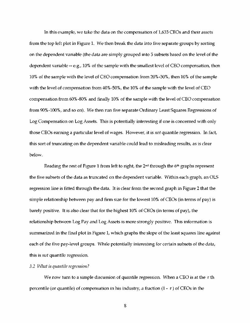
In this example, we take the data on the compensation of 1,633 CEOs and their assets

from the top left plot in Figure 1. We then break the data into five separate groups by sorting

on the dependent variable (the data are simply grouped into 5 subsets based on the level of the

dependent variable -- e.g., 10% of the sample with the smallest level of CEO compensation, then

10% of the sample with the level of CEO compensation from 20%-30%, then 10% of the sample

with the level of compensation from 40%-50%, the 10% of the sample with the level of CEO

compensation from 60%-80% and finally 10% of the sample with the level of CEO compensation

from 90%-100%, and so on). We then run five separate Ordinary Least Squares Regressions of

Log Compensation on Log Assets. This is potentially interesting if one is concerned with only

those CEOs earning a particular level of wages. However, it is not quantile regression. In fact,

this sort of truncating on the dependent variable could lead to misleading results, as is clear

below.

Reading the rest of Figure 1 from left to right, the 2nd through the 6th graphs represent

the five subsets of the data as truncated on the dependent variable. Within each graph, an OLS

regression line is fitted through the data. It is clear from the second graph in Figure 2 that the

simple relationship between pay and firm size for the lowest 10% of CEOs (in terms of pay) is

barely positive. It is also clear that for the highest 10% of CEOs (in terms of pay), the

relationship between Log Pay and Log Assets is more strongly positive. This information is

summarized in the final plot in Figure 1, which graphs the slope of the least squares line against

each of the five pay-level groups. While potentially interesting for certain subsets of the data,

this is not quantile regression.

3.2 What is quantile regression?

We now turn to a simple discussion of quantile regression. When a CEO is at the τth

percentile (or quantile) of compensation in his industry, a fraction (1 - τ) of CEOs in the

8

industry are paid more than he is. If he is at the 5th percentile, 95% of CEOs are paid more; if he

is at the median, then only half are paid more. Koenker and Bassett (1978) extended these ideas

to conditional quantile functions, where quantiles of the conditional distribution of the

dependent variable are expressed as functions of the observed independent variables.

Standard OLS regression is used to obtain estimates for the conditional mean of some

variable, given some set of covariates. One drawback of this approach is that the estimate

obtained is only one number used to summarize the relationship between the dependent

variable and each of the independent variables. In particular, this method assumes that the

conditional distribution is homogenous. This would imply that no matter where you analyze

the conditional distribution, the estimates of the relationship between the dependent variable

and the independent variable are assumed to be the same.

Quantile regression, on the other hand, allows for different estimates to be calculated at

different points on the conditional distribution. In other words, no assumptions about the

homogeneity of the conditional distribution are needed in quantile regression and, in fact,

quantile regression can be used to show that the conditional distribution may not be

homogenous. If estimates at different quantiles are found to be significantly different from one

another, then the conditional distribution is not homogenous.

To be more explicit about the differences between quantile regression and OLS

regression, recall that for OLS, we minimize the following with respect to /? :

" (5) SSE = 2_J(yi -XtP)

i=\

where y is the dependent variable (in our case the log of CEO total annual compensation), X is a

matrix of covariates, and /? is a vector of coefficients. This will give the standard estimates for

the conditional mean of y given X.

9

Quantile regression minimizes not the sum of squared errors, but rather an

asymmetrically weighted sum of absolute errors. Specifically, minimized as:

" ' ' ' 1 (6) 2_1 yi -Xi/3(T)\ • [(T)I(yi > Xi/3(T)) + (1 - r)I(yi < Xi/?(r))J i=

where y is the dependent variable, X is a matrix of covariates, fi is a vector of coefficients which

now depends on r , the quantile being estimated (e.g., r = 0.5 is the median), and the function I

is an indicator function that takes the value of 1 if the condition in the parentheses is true and 0

otherwise. The formula in equation (6) gives weight r to any observations that are above their

respective predicted values and 1 - r weight to any observations that are below their respective

predicted values. This is the same as saying that positive residuals are given weight r and

negative residuals are given weight 1 - r . A special case of this function is conditional median

regression where r = 0.5, since equation (6) collapses to minimizing:

n ' | (7)

2_\yi-Xip\ i=1

which is the standard method for conditional median regression.

Using equation (6), one can estimate /?(r) for any given level of r between 0 and 1.

Thus, we are not making the assumption that estimates at all points on the conditional

distribution are the same (as in OLS) since estimates for /?(r) explicitly depend on the point of

the conditional distribution being estimated ( r ) .

To reiterate, quantile regression is not the same as dividing the data into different

percentiles (or groups) and then running OLS on each percentile. Cutting the data in this way

and then calculating separate estimates means that not all of the data are being used for each

estimate (since only the data from a given group will be used). For each quantile regression

10

estimate, all of the data are being used. However, some observations get more weight than

others.

We can see that quantile regression is a simple extension of the analysis already

presented in Figure 1. In the top left plot in Figure 1, we graphed a single OLS regression line

through the simple cross-section of data from the year 2004 as follows:

{^(compensation) i = p\n(assets)i + si (8)

and our estimate of /? = 0.377. There has been a long history of literature on this simple

relationship between log compensation for managers and log firm size. This literature has

always assumed that there was one return to firm size (e.g., Rosen, 1992). Quantile regression

helps us consider if the return might vary along the conditional distribution of wages. In a

simple quantile regression case, we extend this as follows:

^(compensation) i = PT ln(assets)i + si

where we can estimate separate J3T for any particular quantile. In the case of Figure 2, we do

this for r = 0.10, 0.20, 0.30, 0.40, 0.50 (the median regression), 0.60, 0.70, 0.80, and 0.90. Although

the corresponding quantile regression lines in the left panel of Figure 2 look very similar, they

are not exactly so. In fact, /3T=010 = 0.343, J3T=0 20 = 0.361, J3T=0 30 = 0.359, J3T=0 40 = 0.366, J3T=0 50 =

0.370, J3T=0 60 = 0.360, J3T=0 70 = 0.362, J3T=0 80 = 0.359, a n d J3T=0 90 = 0.362. These coefficients are

plotted against their respective quantiles (along with the horizontal OLS estimate) in the right-

hand panel of Figure 2. Clearly, the slopes increase sharply as we go from the 0.10 quantile up

to the median, and then decline as we go further in the conditional distribution of wages. The

horizontal line in the right-hand panel of figure 2 represents the OLS estimate. It is clear that

there is substantial heterogeneity around this estimate.

11

3.3 Why use quantile regression now and in this context?

Quantile regression may be particularly useful in this context for several reasons. First,

there is a great deal of heterogeneity in the levels of and changes in compensation across firm

types. Similarly, there is wide variation in firm size, however measured, even within the

EXECUCOMP sample used here and described below. This is one of the chief reasons for the

confusion over the standard empirical specification for thinking about CEO pay and firm

performance. Second, although the techniques of quantile regression have existed for some

time, there is now rapid growth in applications. Finally, other researchers (e.g., Schaefer, 1998;

Conyon and Schwalbach, 2000; Baker and Hall, 2004) have shown that there are some

differences in pay for performance sensitivities by different firm characteristics (e.g., firm size).

Quantile regression will allow us to use all of the data at once and to consider whether

there is heterogeneity in the pay-and-performance relationship across the conditional

distribution of wages.

4. The data

In this section, we describe the data and simple descriptive statistics. The data used

here, from Standard & Poor’s EXECUCOMP, are now commonly used in the literature on

executive compensation.

4.1 Basic data description and positive features

The data used in this work are from Standard & Poor’s EXECUCOMP from 1992-2004.

There are several useful features of these data. First, the data include detailed information on

the compensation of the top five highest paid executives over the thirteen-year period. We

focus our attention on the Chief Executive Officer of each firm. Second, the data set is large and

contains information from about 1,500 firms for each of the thirteen years of the sample. Third,

12

since the data contain information from a wide variety of firms (Standard & Poor’s 500-stock

index, Standard & Poor’s Mid-Cap 400, and SmallCap 600 there is considerable variation in firm

size which will prove useful.

4.2 Sample descriptive statistics

We consider 17,403 CEO-year observations in the main part of our analysis. Table 1

shows that for the entire sample period, the median CEO had salary and bonus of $750,000 and

total compensation (including the Black-Scholes value of stock options at the time of grant) of

$1,688,000. Median sales in these firms is $908 Million, and the median market value of equity

in the firms is $1.03 Billion. Descriptive statistics for all variables in each of the years from 1992

- 2004 are also reported in Table 1.

5. Is there heterogeneity in the pay-for-performance relationship?

Although it is clear from the right-hand panel of Figure 2 that there is heterogeneity in

the return to firm size (as measured by assets), this section is specifically focused on considering

heterogeneity in the pay-for-performance relationship. We do this by simply extending the

model introduced in Section 2.2 to the quantile regression context. We then compute the return

across the quantiles of the conditional distribution of compensation for the managers.

5.1 Heterogeneity in Murphy’s (1986) specification?

A very well-known specification we investigate is that of Murphy (1986). We have only

slightly modified this specification so that the pay-for-performance sensitivity (/?) can vary by

the quantiles, r . We denote this in equation (10) as f3t

Aln(compensation)it =6 + j3TAln(firm value)it + rjit (10)

13

Table 2 presents the results from ten different estimates of the pay-for-performance relationship

with the change in the natural log of salary and bonus plus the value of options granted in a

given year as the dependent variable. The numbers for the quantile regression estimates can be

interpreted as conditional on a set of covariates: if a CEO is expected to lie in the x-th quantile of

the wage distribution, then the estimated pay for performance sensitivity equals pT. For

example, the coefficient estimate on change in shareholder value in Table 2 for the 10% quantile

implies that given the set of covariates, a CEO in the 10th percentile of the conditional wage

distribution is expected to have a pay-for-performance sensitivity of -0.0074. It is clear that the

OLS (/? = 0.0673) and median regression (fiT=050 = 0.0580) estimates are somewhat similar.

However, it is also clear that as the quantiles increase so do the pay-for-performance

sensitivities. This is easily seen in Figure 3, which plots each of the ten quantile regression

estimates from Table 2 (along with the 95% confidence intervals). From this picture we can see

that conditionally low-wage CEOs have a smaller pay-for-performance sensitivity than

conditionally high-wage CEOs.4 If we assume that conditionally high-wage CEOs are typically

“higher quality managers,” then these results would suggest that firms tie CEO pay with

performance more tightly when the CEO is of higher quality. This could make sense since

higher quality CEOs would tend to give the firm high return on their effort. Therefore,

inducing higher effort from the CEO by linking pay to firm performance would outweigh the

cost to the firm of monitoring CEO effort if the CEO is high quality. These results would also

suggest that linking pay to performance for low-conditional-wage CEOs may not be as

profitable for the firm for similar reasons. The results in Table 2 would also coincide with the

explanation suggested in section I.C, where high ability CEOs have higher pay-for-performance

4 This discussion supposes that /? measures the relationship between compensation and firm value. This

is exactly what equation (10) is doing since (10) is just a variant of (1) with the unobserved fixed effect, yi,

removed. Differencing as in either (4) or (10) is essentially running a fixed-effects model like (1).

14

sensitivities than low ability CEOs if ability is positively related to conditional wages. This is

likely to be the case but cannot be formally tested in this setting without some measure for

ability. In order for these results to match an explanation based on risk aversion, one would

have to argue that high-conditional-wage CEOs tend to have lower risk aversion than low-

conditional-wage CEOs. Since we doubt that it is the case that risk aversion differs in this way

across CEOs, we cannot say whether this explanation for heterogeneity is valid given our

results.

The next obvious question is whether the returns to performance differ significantly

across quantiles. For example, in specification (10), w e get /3T=010 = -0.0074 and /3T=0 50 = 0.0580.

The general procedure for hypothesis testing used here to establish a case for heterogeneity is

based on the work of Koenker and Bassett (1982) and Hendricks and Koenker (1991). Tests of

hypotheses that take the form H0: A-i = Pn against H1: Pr\ * Pn can be written as:

Tn = {flTl - pv2)' (H~lJH~l yl {flTl - pT2) (11)

where H 1 JH 1 is the “sandwich” formula used in Hendricks and Koenker (1991). This test has

an asymptotic F distribution when it is divided by its degrees of freedom. This form of the test

can be used to either test a vector of coefficients across a pair of quantiles or to test a single

coefficient across a pair of quantiles. In the case of a single coefficient, this statistic simplifies to:

rji \Pv,T\~Pv,Tl)~\Pv,T\~Pv,Tl) ( ) ln = , ^

•\f * \Pp,T\ > + " (Pp,T2> ~ ^OV(Pp,Tl J Pp,T2 )

where p is the variable of interest and fip^ (where i = 1,2) is the coefficient estimate at a given

quantile for the variable. This version of the formula may be a bit more intuitive since it looks

similar to the standard tests for differences in means. Instead of using this form to test for

15

differences in means, we are using a similar procedure to test for differences in conditional

quantile estimates.

These tests can be used to establish a case for heterogeneity because if the null

hypothesis is rejected, we can conclude that there are significant differences across quantiles.

Given that these differences are significant, this would suggest that there is evidence that the

pay-for-performance sensitivity is different at different points in the conditional distribution

(i.e., there is significant heterogeneity in pay-for-performance sensitivities across the conditional

wage distribution).

Table 3 shows the results of tests for significant differences for all possible cases outlined

in Table 2. For example, the F-statistic for testing whether there is a significant difference

between /?r=0 1 and /3T=0 5 is 28.320, which is significant at the 1% level. In fact, all of the

coefficients are significantly different from one another. This implies that significant

heterogeneity exists in pay for performance sensitivities using the Murphy (1986) specification.

5.2 Relation with other pay-for-performance work

Conyon and Schwalbach (2000) also investigate a type of heterogeneity in the pay-for-

performance relationship using data from the UK and Germany, but they do not use quantile

regression. Instead, the authors estimate a separate pay-for-performance sensitivity for every

firm in their data set, and then consider the distribution of those estimates. In other words, they

examine the distribution across firms of conditional mean estimates of within-firm pay-for-

performance sensitivities. Using our data, we use a similar method in Figure 4 to document the

types of differences in sensitivities pointed out by Conyon and Schwalbach in the UK and

Germany. We ran specifications like equation (4) (analogous to Figure 3 and Tables 2 and 3)

1,585 times. The 1,585 represents the number of firms for which we have data for three

16

consecutive years. In Figure 4, we plot the distribution of within-firm returns5, with 4.2%

(median 6.1%) with wide variability.

Though our example of the Conyon and Schwalbach (2000) method shows a form of

heterogeneity in the pay-for-performance relationship, this is not the same as the heterogeneity

shown using quantile regression. The estimates from the quantile regressions used in our paper

suggest heterogeneity in the pay-for-performance sensitivity across the conditional distribution

of wages, not across firms, as in Conyon and Schwalbach.

Other recent work on the firm size effect and CEO pay include Baker and Hall (2004)

and Schaefer (1998). Baker and Hall find that firm size has different effects on different

measures of CEO incentives, and they attempt to show under which circumstances each

measure of incentives should be used for analysis. Specifically, they find that if activities have

dollar impact that is the same across different firm sizes, then the measure of CEO incentives

should be the CEO’s “percent owned”; and if activities have percentage returns that are

constant across firm size, then the CEO’s “equity stake” should be used. Schaefer (1998)

develops a model based on agency theory that includes both costs of effort by the CEO and risk

aversion and uses this model to examine the effect of firm size on pay-for-performance

sensitivities. He finds that pay-for-performance sensitivity is inversely proportional to the

square root of firm size, independent of how firm size is measured. Rather than distinguishing

among different theories of compensation, our goal is to empirically examine executive pay

using quantile regression. Our hope is that quantile regression techniques will ultimately be

helpful in contributing to this literature as well.

2.6% of the returns are outside of the bounds in the figure.

17

6. Concluding comments and future work

There is a lot of interesting literature on the economics of executive compensation.

Much of this work has concentrated on the relationship between the pay of the top manager

and the performance of the firm. Even more recent work has suggested that the relationship

between pay and performance in firms is not constant across all firm types (e.g., Schaefer, 1998;

Conyon and Schwalbach, 2000; Baker and Hall, 2004).

This paper uses quantile regression techniques developed by Koenker and Bassett (1978)

to investigate whether there is heterogeneity in the pay-for-performance link across the

conditional distribution of wages for managers of U.S. firms over the years 1992 – 2004. The

results suggest that for some commonly used specifications in the literature, there is

considerable heterogeneity in returns to firm performance across the conditional distribution of

wages. But what is the fundamental source of this heterogeneity? There are several possible

sources, such as firm risk, firm beta, managerial ability, managerial risk aversion, and the shape

of the firm’s age-wage profiles. Each of these is a potential fruitful area for future work.

These ideas can be extended to many other areas. One is in the area of management

turnover. The theory of quantile regression has only recently been extended to the case of

binary response variables (Kordas, 2000). With this, ideas from the extensive literature on CEO

turnover could be explored in the quantile regression context. Another area of interest is

relative performance evaluation of CEOs. We expect that quantile regression will continue to be

used in these and many other interesting areas.

18

References

Aggarwal, Rajesh K. and Andrew Samwick, 1999. The other side of the trade-off: The impact of risk on executive compensation, Journal of Political Economy 107, 65-105.

Baker, George and Brian Hall, 2004. CEO incentives and firm size, Journal of Labor Economics 22, 767-798.

Core, John E., 2002. Discussion of the roles of performance measures and monitoring in annual governance decisions in entrepreneurial firms, Journal of Accounting Research 40, 519-527.

Conyon, Martin and Joachim Schwalbach, 2000. Executive compensation: Evidence from the UK and Germany, Long Range Planning 33, 504–526.

Coughlan, Anne T. and Ronald M. Schmidt, 1985. Executive compensation, management turnover, and firm performance: An empirical investigation, Journal of Accounting and Economics 7, 43-66.

Engel, Ellen, Elizabeth A. Gordon, and Rachel M. Hayes, 2002. The roles of performance measures and monitoring in annual governance decisions in entrepreneurial firms, Journal of Accounting Research 40, 485-518.

Fama, Eugene, 1980. Agency problems and the theory of the firm, Journal of Political Economy 88, 288–307.

Grossman, Sanford and Oliver Hart, 1983. An analysis of the principal-agent problem, Econometrica 51, 7–45.

Hall, Brian and Jeffrey Liebman, 1998. Are CEOs really paid like bureaucrats? Quarterly Journal of Economics CXXIII, 653-692.

Hallock, Kevin F. and Kevin J. Murphy, 1999. The Economics of Executive Compensation. (Edward Elgar Publishing Limited, Cheltenham England and Northampton Massachusetts).

Hallock, Kevin F. and Paul Oyer, 1999. The timeliness of performance information in determining executive compensation, Journal of Corporate Finance 5, 573–577.

Hendricks, Wallace and Roger Koenker, 1991. Hierarchical spline models for conditional quantiles and the demand for electricity, Journal of the American Statistical Association 87, 58-68.

Holmstrom, Bengt, 1979. Moral hazard and observability, Bell Journal of Economics 10, 74–91.

Holmstrom, Bengt and Paul Milgrom, 1987. Aggregation and linearity in the provision of intertemporal incentives, Econometrica 55, 303–328.

19

Jensen, Michael and William Meckling, 1976. Theory of the firm: Managerial behavior, agency costs, and ownership structure, Journal of Financial Economics 3, 305-360.

Jensen, Michael, C. and Kevin J. Murphy, 1990. Performance pay and top management incentives, Journal of Political Economy 98, 225-264.

Koenker, Roger and Gilbert Bassett, 1978. Regression quantiles, Econometrica 46, 33-50.

Koenker, Roger and Gilbert Bassett, Jr., 1982. Robust tests for heteroscedasticity based on regression quantiles, Econometrica 50, 43-63.

Koenker, Roger and Kevin F. Hallock, 2001. Quantile regression, Journal of Economic Perspectives 15, 143-156.

Kordas, Gregory, 2000. Binary quantile regression. Ph.D. Dissertation, University of Illinois.

Lazear, Edward and Sherwin Rosen, 1981. Rank-order tournaments as optimum labor contracts, Journal of Political Economy 89, 841-864.

Lewellen, Wilbur G. and Blaine Huntsman, 1970. Managerial pay and corporate performance, American Economic Review 60, 710-720.

Murphy, Kevin J., 1985. Corporate performance and managerial remuneration: An empirical analysis, Journal of Accounting and Economics 7, 11-42.

Murphy, Kevin J., 1986. Incentives, learning, and compensation: A theoretical and empirical investigation of managerial labor markets, Rand Journal of Economics 17, 59-76.

Murphy, Kevin J., 1999. Executive Compensation, in Orley Ashenfelter and David Card, Editors, Handbook of Labor Economics, Volume 3B. (Elsevier Science Publishers, 2485-2563).

Rosen, Sherwin, 1992. Contracts and the Market for Executives, in Lars Werin and Hans Wijkander, Editors, Contract Economics, Chapter 7, 181-211. (Blackwell, Oxford).

Schaefer, Scott, 1998. The Dependence of Pay-Performance Sensitivity on the Size of the Firm, Review of Economics and Statistics, 436-443.

Weisbach, Michael, S., 1988. Outside directors and CEO turnover, Journal of Financial Economics 20, 431-460.

20

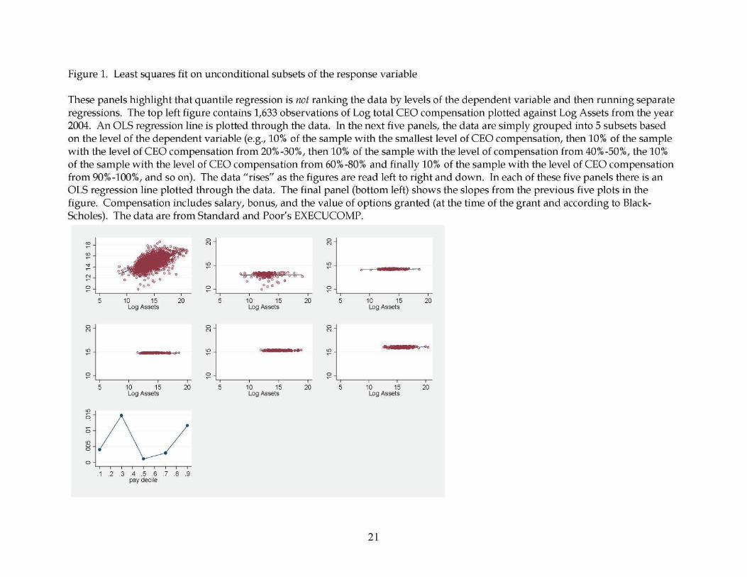
Figure 1. Least squares fit on unconditional subsets of the response variable

These panels highlight that quantile regression is not ranking the data by levels of the dependent variable and then running separate regressions. The top left figure contains 1,633 observations of Log total CEO compensation plotted against Log Assets from the year 2004. An OLS regression line is plotted through the data. In the next five panels, the data are simply grouped into 5 subsets based on the level of the dependent variable (e.g., 10% of the sample with the smallest level of CEO compensation, then 10% of the sample with the level of CEO compensation from 20%-30%, then 10% of the sample with the level of compensation from 40%-50%, the 10% of the sample with the level of CEO compensation from 60%-80% and finally 10% of the sample with the level of CEO compensation from 90%-100%, and so on). The data “rises” as the figures are read left to right and down. In each of these five panels there is an OLS regression line plotted through the data. The final panel (bottom left) shows the slopes from the previous five plots in the figure. Compensation includes salary, bonus, and the value of options granted (at the time of the grant and according to Black-Scholes). The data are from Standard and Poor’s EXECUCOMP.

21

Figure 2. Quantile regressions of log compensation on log assets

The left-hand panel contains 1,633 observations of Log total CEO compensation plotted against Log assets from the year 2004. Quantile regression lines from nine quantile regressions (at 0.10, 0.20, 0.30, 0.40, 0.50, 0.60, 0.70, 0.80, and 0.90) are plotted through the data in the left-hand panel of the figure (the 10th quantile is the bottom line all the way up to the 90th which is the top line). The right-hand figure depicts the nine slopes on Log Assets from the nine quantile regressions, along with the least squares line (horizontal). Compensation includes salary, bonus, and the value of options granted (at the time of the grant and according to Black-Scholes). The data come from Standard and Poor’s EXECUCOMP.

22

Figure 3. Quantile regression estimates of /3T

The empirical model estimated is Aln(compensation)it = 6 + j3TAln(firm value)it. Compensation includes salary, bonus, and the

value of options granted (at the time of the grant and according to Black-Scholes). The horizontal lines represent the OLS estimate and the 95% confidence intervals. The dots represent the nine quantile regression estimates and corresponding confidence intervals. Data are from Standard and Poor’s EXECUCOMP, 1992-2004.

23

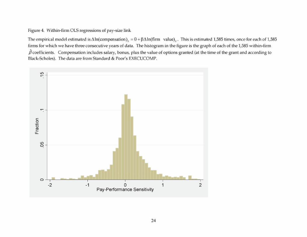
Figure 4. Within-firm OLS regressions of pay-size link

The empirical model estimated is Aln(compensation)it = 9 + |3Aln(firm value) l t. This is estimated 1,585 times, once for each of 1,585

firms for which we have three consecutive years of data. The histogram in the figure is the graph of each of the 1,585 within-firm

P coefficients. Compensation includes salary, bonus, plus the value of options granted (at the time of the grant and according to

Black-Scholes). The data are from Standard & Poor’s EXECUCOMP.

Pay-Performance Sensitivity

24

Table 1. Summary statistics, medians

Median statistics for companies and CEOs are reported overall and by year from 1992-2004. Data are presented on salary and bonus, total compensation (including the value of options granted), sales, assets market value and return on assets). All data in table are medians except for sample sizes. Data only include information for CEOs. Samples sizes are for compensation. The data are from Standard and Poor’s EXECUCOMP. (a) In thousands. (b) In millions.

Total 1992 1993 1994 1995 1996 1997 1998 1999 2000 2001 2002 2003 2004 The CEO Salary + bonus(a) 745 483 500 554 576 650 675 672 746 810 810 920 1,008 1,239

Total compensation(a)

The firm Sales(b)

1,688 785 854 968 1,036 1,253 1,460 1,574 1,930 2,186 2,345 2,393 2,424 3,036

908 599 595 645 707 728 788 834 944 1,053 1,089 1,039 1,136 1,345

Assets(b) 1,154 943 754 783 852 862 916 993 1,127 1,308 1,381 1,412 1,555 1,818

Market value(b) 1,027 573 603 578 732 813 1,027 947 1,091 1,176 1,273 1,062 1,493 1,816

Return on assets 3.94 3.67 3.99 4.25 4.18 4.52 4.64 4.01 4.30 4.28 2.91 3.14 3.45 4.25 (%)

N 17,403 678 954 1,040 1,118 1,281 1,388 1,474 1,490 1,496 1,530 1,628 1,676 1,630

25

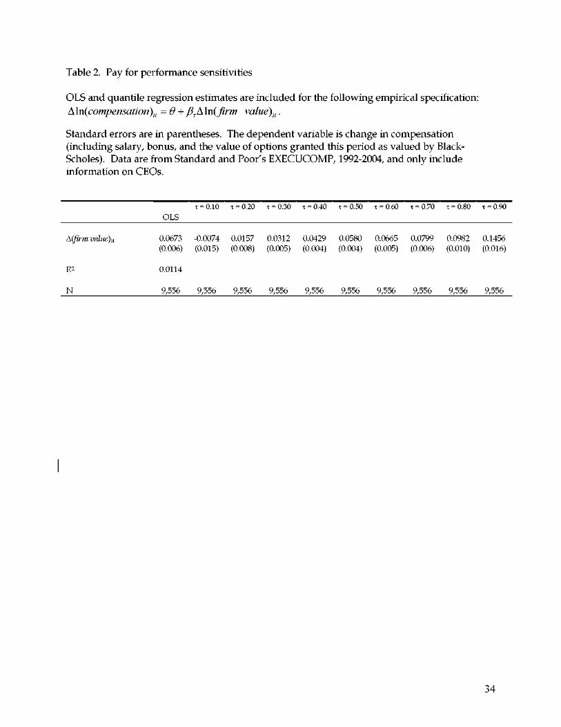
Table 2. Pay for performance sensitivities

OLS and quantile regression estimates are included for the following empirical specification: A\n(compensation)it =6 + J3TAln( firm value)it.

Standard errors are in parentheses. The dependent variable is change in compensation (including salary, bonus, and the value of options granted this period as valued by Black-Scholes). Data are from Standard and Poor’s EXECUCOMP, 1992-2004, and only include information on CEOs.

x = 0.10 x = 0.20 x = 0.30 x = 0.40 x = 0.50 x = 0.60 x = 0.70 x = 0.80 x = 0.90 OLS

A(firm value)it 0.0673 -0.0074 0.0157 0.0312 0.0429 0.0580 0.0665 0.0799 0.0982 0.1456

(0.006) (0.015) (0.008) (0.005) (0.004) (0.004) (0.005) (0.006) (0.010) (0.016)

R2 0.0114

N 9,556 9,556 9,556 9,556 9,556 9,556 9,556 9,556 9,556 9,556

34

Table 3. F statistics for differences in slopes across quantiles

This table reports F statistics for testing across specifications in Table 2. All combinations are significantly different from one another at the 1% level.

x = 0.10 x = 0.20 x = 0.30 x = 0.40 x = 0.50 x = 0.60 x = 0.70 x = 0.80

x = 0.20 6.988

-------

x = 0.30 14.628 13.033

------

x = 0.40 22.103 26.541 18.221

-----

x = 0.50 28.320 37.979 33.203 17.411

----

x = 0.60 43.685 69.623 78.564 73.810 59.803

---

x = 0.70 54.066 76.116 70.455 52.257 38.341 11.379

--

x = 0.80 80.130 134.010 153.120 147.680 127.210 70.528 19.825

-

T = 0.90 91.950 100.510 88.732 75.269 65.976 48.315 38.540 22.471

35