Single-index quantile regression

Journal of Multivariate Analysis 101 (2010) 1607–1621

Contents lists available at ScienceDirect

Journal of Multivariate Analysis

journal homepage: www.elsevier.com/locate/jmva

Single-index quantile regressionI

Tracy Z. Wu a, Keming Yu b, Yan Yu c,∗a Consumer Risk Modeling and Analytics Group at JPMorgan Chase Bank, 1111 Polaris Parkway, Columbus, OH 43240, United Statesb Brunel University, Uxbridge, Middlesex UB8 3PH, London, UKc University of Cincinnati, PO BOX 210130, Cincinnati, OH 45221, United States

a r t i c l e i n f o

Article history:Received 25 March 2009Available online 19 February 2010

AMS subject classifications:62G0862G2062G35

Keywords:Conditional quantileDimension reductionLocal polynomial smoothingNonparametric modelSemiparametric model

a b s t r a c t

Nonparametric quantile regression with multivariate covariates is a difficult estimationproblem due to the ‘‘curse of dimensionality’’. To reduce the dimensionality while stillretaining the flexibility of a nonparametric model, we propose modeling the conditionalquantile by a single-index function g0(xTγ0), where a univariate link function g0(·) isapplied to a linear combination of covariates xTγ0, often called the single-index. Weintroduce a practical algorithmwhere the unknown link function g0(·) is estimated by locallinear quantile regression and the parametric index is estimated through linear quantileregression. Large sample properties of estimators are studied, which facilitate furtherinference. Both the modeling and estimation approaches are demonstrated by simulationstudies and real data applications.

© 2010 Elsevier Inc. All rights reserved.

1. Introduction

In this paper, we introduce single-index quantile regression for nonparametric estimation with multivariate covariates.Given τ ∈ (0, 1), we propose a single-index model for the τ th conditional quantile θτ (x) of y given x,

θτ (x) = g0(xTγ0), (1)

where x is a vector of d-dimensional covariates, y is a real valued dependent variable, g0(·) is the unknown univariate linkfunction, and γ0 is the unknown single-index vector coefficient satisfying ‖γ0‖ = 1 and the first component γ1 > 0 foridentifiability [1]. Here ‖ · ‖ is the Euclidean norm. Single-index quantile regression model (1) generalizes the seminal workof linear quantile regression of Koenker and Bassett [2] by replacing the linear combination xTγ0 with a nonparametriccounterpart g0(xTγ0).The single-index approach has proven to be an efficient way to cope with high-dimensional nonparametric estimation

problems in conditional mean regression (e.g. [3–8]). When used to model conditional quantiles involving multivariatecovariates, single-index models inherit the same advantages as in the mean regression context: (i) the unspecified linkfunction allowsmodel flexibility and thus has less risk of mis-specification; (ii) the single-index in the link function projectsmultivariate covariates onto one-dimensional variate, effectively reducing the dimensionality in nonparametric estimation;(iii) the single-index structure together with the nonlinear link function can model some interactions among the covariates

I This manuscript is based in part on the Ph.D. Thesis of the first author at University of Cincinnati. This paper formerly circulated under the title ‘‘LocalLinear Estimation for Single-index Conditional Quantiles’’, which was presented in JSM in Seattle, August 2006.∗ Corresponding address: Department of Quantitative Analysis OperationsManagement, University of Cincinnati, PO BOX 210130, Cincinnati, OH 45221,United States.E-mail address: [email protected] (Y. Yu).

0047-259X/$ – see front matter© 2010 Elsevier Inc. All rights reserved.doi:10.1016/j.jmva.2010.02.003

http://www.elsevier.com/locate/jmva

http://www.elsevier.com/locate/jmva

mailto:[email protected]

http://dx.doi.org/10.1016/j.jmva.2010.02.003

1608 T.Z. Wu et al. / Journal of Multivariate Analysis 101 (2010) 1607–1621

implicitly, which is more realistic to real applications; (iv) the interpretation of covariate effects is easy because of the linearstructure of the index. Model (1) is very general. Under certain assumptions (e.g. monotonicity) the model can be used tomodel the quantiles for several important cases such as survival and transformation models and location-scale model, aspointed out in [9]. These cases would be interesting for future research. Indeed, based on our estimation equation (6), Kongand Xia [10] recently investigated the Bahadur representation of single-index parameter estimators.Research on nonparametric quantile regression is relatively sparse in contrast to that for mean regression. Yu and

Jones [11] developed local linear approaches for univariate quantile regression. Besides local estimation approaches, splineapproach is another stream of nonparametric quantile regression. See [12,13] for more details. Stone [14] and Chaudhuri[15] considered fully nonparametric quantile regression in a general multivariate setting. They are flexible but usuallyunattractive in practice due to the well-known ‘‘curse-of-dimensionality’’.Recently, dimension-reduction techniques for nonparametric quantile regressionmodels have attracted a lot of attention

in the literature. These include additive models and partially linear models (e.g. [16–18]). But these models do notincorporate interactions, nor nest with single-index models. A close alternative to our approach is the important work ofaverage derivativemodels (e.g. Chaudhuri et al. [9] for quantile regression; Härdle and Stoker [19] formean regression). Theyestimate the single-index vector by taking an expectation of the vector of partial derivatives of the conditional quantile withrespect to the covariates x. Though theoretically appealing, it requires relevant multi-dimensional quantiles to be obtainednonparametrically before the index can be estimated directly.In this article, we present an overall treatment of estimation and inference along with an application using the proposed

single-index quantile regression model (1). To the best of our knowledge, this appears to be the first paper in the scientificliterature that presents a comprehensive study of single-index quantile regression. In practice, we introduce an algorithmthat is particularly tailored to model (1), which is based on the local linear approach to estimate the nonparametric partg0(·), and linear quantile regression to solve the parametric index part γ0. With this algorithm, single-index models can beestimated quite expediently as shown in both simulation study and real data applications. It is natural to adopt the locallinear approach as in Yu and Jones[11] for univariate conditional quantiles. Not surprisingly, Yu and Jones [20] also findthat local linear method is more advantageous over local constant approaches in quantile regression because of their lowerbias and nicer boundary performances. In theory, we obtain the asymptotic properties for the proposed nonparametricestimator g(·), conditional quantile estimator θτ (x), and the parametric single-index vector estimate γ, which naturallyfacilitate further inference. Confidence intervals for conditional quantiles are also readily available. In addition, we derive anapproximate simple-to-calculate rule-of-thumb bandwidth selector based on the large sample theory. Optimal bandwidthbyminimizing the asymptotic mean squared error for single-index quantile regressionmight be otherwise computationallyintensive, particularly when a number of quantiles need to be estimated. AMonte Carlo simulation study and an applicationto Boston Housing data show promises of our proposed approach.The rest of the paper is organized as follows. In Section 2, we propose a local linear estimation method as well as some

computational algorithms. Asymptotic properties of the estimators are obtained in Section 3. We present both simulationexamples and real data applications in Section 4. Section 5 concludes the paper. All the proofs are relegated to the Appendix.

2. The model and estimation

2.1. The model and local linear estimation

For our single-index quantile regression model (1), note g0(·) should really be g0,τ (·) and γ0 should be γ0,τ , both uniqueto the given quantile. We omit the subscript τ for notational convenience. The linear combination of the covariates xTγ0 isoften called the single-index. Mathematically, the true parameter vector γ0 solves the following minimization problem:

γ0 = argminγE[ρτ(y− g(xTγ)

)]subject to ‖γ‖ = 1, γ1 > 0, (2)

where the loss function (also called the ‘‘check’’ function) ρτ (u) = |u| + (2τ − 1)u and g(·) is the unknown link function.The right-hand side of the above equation is the expected loss which can be equivalently written as

E[ρτ(y− g(xTγ)

)]= E

{E[ρτ(y− g(xTγ)

)|xTγ

]}, (3)

where E[ρτ(y− g(xTγ)

)|xTγ

]is the conditional expected loss and g(·) is the τ th conditional quantile function.

Let {xi, yi}ni=1 be an independent identically distributed (i.i.d.) sample from (x, y). For xTi γ ‘‘close’’ to u, the τ th conditional

quantile at xTi γ can be approximated linearly by

g(xTi γ) ≈ g(u)+ g

′(u)(xTi γ− u) = a+ b(x

Ti γ− u), (4)

where adef≡ g(u) and b

def≡ g ′(u). Following (4), we minimize the following local linear sample analogue of Lγ(u) [11] with

respect to (a, b) to obtain g(u) = a,n∑i=1

ρτ(yi − a− b(xT

i γ− u))K(xTi γ− uh

), (5)

where K(·) is the kernel weight function and h is the bandwidth.

T.Z. Wu et al. / Journal of Multivariate Analysis 101 (2010) 1607–1621 1609

We average (5) over u and obtain the sample analog of (3), i.e. the objective function that is used to estimate model (1),

n∑j=1

n∑i=1

ρτ(yi − aj − bj(xT

i γ− xTj γ)) Kh(xT

i γ− xTj γ)

n∑l=1Kh(xT

l γ− xTj γ)

, (6)

whereKh(·) = K(·/h)/h. In practice,minimization of (6) is done by iteratively solving two simple problems, onewith respectto aj’s and bj’s, and the other with respect to γ.We rewrite (6) as

n∑j=1

n∑i=1


i γ− xTj γ))ωij, (7)

where ωij =Kh(xTi γ−x

Tj γ)∑n

l=1 Kh(xTl γ−x

Tj γ). We decompose (7) into:

P1. Given γ,

(aj, bj)nj=1 = arg min(aj,bj)nj=1

n∑j=1

n∑i=1


i γ− xTj γ))ωij.

So for any j ∈ {1, 2, . . . , n},

(aj, bj) = arg min(aj,bj)

n∑i=1


i γ− xTj γ))ωij.

P2. Given aj’s and bj’s,

γ = argminγ

n∑j=1

n∑i=1

ρτ(yi − aj − bj(xi − xj)Tγ

)ωij

= argminγ

n∑j=1

n∑i=1

ρτ(y∗ij − x∗ij

Tγ)ω∗ij,

where y∗ij = yi − aj, x∗

ij = bj(xi − xj), and ω∗ij = ωij evaluated at the current estimate of γ, i, j = 1, . . . , n.

The subproblem P1 deals with estimating (aj, bj), j = 1, . . . , n, as if γ is known. While in P2, γ is estimated throughusual linear quantile regression without intercept (regression-through-origin) on n2 ‘‘observations’’ {y∗ij, x

∗

ij}ni,j=1 with known

weights {ω∗ij}ni,j=1 evaluated at the estimate of γ from the previous iteration.

An algorithm for estimating γ is as follows.

Step 0. Obtain initial γ(0) from average derivative estimate (ADE) of Chaudhuri et al. [9]. Standardize the initial estimatesuch that ‖γ‖ = 1 and γ1 > 0 (Initialization step).

Step 1. Given γ, obtain {aj, bj}nj=1 by solving a series of the following

min(aj,bj)

n∑i=1

ρτ(yi − aj − bj(xi − xj)Tγ

)ωij, (8)

with the bandwidth h chosen optimally.Step 2. Given {aj, bj}nj=1, obtain γ by solving

minγ

n∑j=1

n∑i=1

ρτ

(yi − aj − bj(xi − xj)Tγ

)ωij, (9)

with ωij evaluated at γ and h from step 1.Step 3. Repeat Steps 1 and 2 until convergence.

In the above algorithm, γ is standardized this way: γ = sign1γ/‖γ‖, where sign1 is the sign of the first component of γ.Only a starting value for γ is needed. The initial estimator γ(0) from average derivative estimate (ADE) of Chaudhuri et al. [9]has nice properties and has been proven to be root-n consistent. However, multi-dimensional kernel estimation is involved,which may be computationally intensive. Alternatively, in practice, one may obtain initial γ(0) from mina,γ

∑ni=1 ρτ (yi −

a − xTi γ), where a is the quantile regression intercept. A similar algorithm was introduced by Xia et al. [21] in the mean

regression context.


Finally, we estimate g(·) at any u by g(·; h, γ) = awhere

(a, b) = argmin(a,b)

n∑i=1


i γ− u))Kh(xT

i γ− u). (10)

A program written in the R environment which executes the algorithm is downloadable from the following linkhttp://statqa.cba.uc.edu/~yuy/SINDEXQ.rar.

2.2. Selection of bandwidth

Bandwidth selection is always crucial in local smoothing as it governs the curvature of the fitted function. Theoretically,when the sample size is large, the optimal bandwidth could be derived by minimizing the asymptotic mean squared error(AMSE) from Theorem 1 in Section 3.1. However, the optimal bandwidth can not be calculated directly due to severalunknownquantities. Implementation is also computationally expensive, particularlywhenwewould like to estimate severalquantiles. Yu and Jones [11] derived an approximate optimal bandwidth under moderate assumptions. In fact, by notingthat the similarities between our AMSE and the expression given by Yu and Jones [11] and following the same argument,we obtain the following rule-of-thumb bandwidth hτ :

hτ = hm{τ(1− τ)/φ

(8−1(τ )

)2}1/5, (11)

where φ(·) and 8(·) are the probability density function and the cumulative distribution function of the standardnormal distribution respectively. The bandwidth hτ has a nice property of relating to the optimal bandwidth hm ={

[∫K2(v)dv][var(y|xTγ=u)]

n[∫v2K(v)dv]2[ d

2

du2E(y|xTγ=u)]2[fU0 (u)]

}1/5used inmean regression via amultiplying factor involving only τ . Since there aremany

existing algorithms for hm (see e.g. [22]), hτ is also readily available.The approximation by (11) provides a computationally easy way to calculate the otherwise difficult-to-obtain optimal

bandwidth for quantile regression. However, the approximation is based on several key assumptions, notably among whichare that the curvatures of the conditional median and the conditional mean are similar and that the conditional densityfunction of the dependent variable can be approximated by normal densities. Details regarding the approximation can befound in [11,17].

3. Large sample properties

3.1. Asymptotics for nonparametric part

This section aims to derive the distribution theory for the nonparametric estimator g(·). This requires that γ0 is eithergiven or estimated with reasonable accuracy. A degenerate case of scalar γ0 has been addressed in [23,11].We assume that the parametric part γ can be estimated to the order Op(n−1/2). Indeed, the root-n consistent average

derivative quantile estimator (ADE, [9]) is used as ‘‘pilot’’ estimator γ(0), though initial multi-dimensional smoothing is

involved. The root-n neighborhood assumption is common in single-index mean regression literatures, see e.g. [24,6]. Thefinal estimator of the nonparametric part is obtained byminimizing (10) and can be as efficient as the casewhenγ0 is known.Assumptions

(i) The kernel K(·) ≥ 0 has a compact support and its first derivative is bounded. It satisfies∫∞

−∞K(z)dz = 1,∫

∞

−∞zK(z)dz = 0,

∫∞

−∞z2K(z)dz <∞, and |

∫∞

−∞z jK 2(z)dz| <∞, j = 0, 1, 2.

(ii) The density function of xTγ is positive and uniformly continuous for γ in a neighborhood of γ0. Further the densityof xTγ0 is continuous and bounded away from 0 and∞ on its support.

(iii) The conditional density function of y given u, fy(y|u) is continuous in u for each y. Moreover, there exist positiveconstants ε and δ and a positive function G(y|u) such that

sup|un−u|≤ε

fy(y|un) ≤ G(y|u) and that∫|ρ ′τ (y− g0(u))|

2+δG(y|u)dµ(y) <∞, and∫(ρτ (y− t)− ρτ (y)− ρ ′τ (y)t)

2G(y|u)dµ(y) = o(t2) as t → 0.

(iv) The function g0(·) has a continuous and bounded second derivative.

The assumptions above are commonly used in the literature and are satisfied in many applications. Assumption (i)simply requires that the kernel function is a proper density with finite second moment that is required for the asymptoticvariance of estimators; Assumption (ii) guarantees the existence of any ratio terms with the density appearing as part ofthe denominator; Assumption (iii) is weaker than the Lipschitz continuity of the function ρ ′τ (·); Assumption (iv) is acommon assumption for a link function.

http://statqa.cba.uc.edu/~yuy/SINDEXQ.rar


Remark 1. (i) The loss function ρτ (·) is piecewise linear and non-differentiable at 0. We have ρ ′τ (y) = 2(τ − I(y < 0))at y 6= 0 and may set ρ ′τ (y) = 0 at y = 0. In fact, for any continuous random variable y, y = 0 occurs with a zeroprobability.

(ii) Since ρ ′τ (·) is piecewisely constant with limited number of values, the condition∫|ρ ′τ (y− g0(u))|

2+δG(y|u)dµ(y) <∞ in Assumption (iii) can be reduced to

∫G(y|u)dµ(y) <∞.

Theorem 1. Under Assumptions (i)–(iv), if n→∞, h→ 0, and nh→∞, then for an interior point u,

(nh)1/2{g(u; h, γ)− g0(u)− β(u)h2}D→ N(0, α2(u)),

where β(u) = g ′′0 (u)∫v2K(v)dv2 , α2(u) =

∫K2(v)dvfU0 (u)

τ (1−τ)[fy(g0(u)|u)]2

, fU0(·) is the density of U0 = xTγ0 and fy(·|u) is the conditionaldensity of y given u.Proof. See Appendix. �

In Theorem 1, we consider the difference between the estimated link function and true link function, both evaluatedat the same index value u. However pointwise accuracy is based on the quantity θτ (x) − θτ (x) = g(xTγ; γ) − g0(xTγ0).Here both the estimated link function and true link function are evaluated at the same covariate value x, while the quantileestimate takes both index coefficient and link function as estimated. The scaled pointwise error term can be written as(nh)1/2{θτ (x) − θτ (x)} = (nh)1/2{g(xTγ; γ) − g(xTγ0; γ)} + (nh)

1/2{g(xTγ0; γ) − g0(xTγ0)}, where g(xTγ; γ) is g(·; γ)

evaluated at xTγ and g(xTγ0; γ) is g(·; γ) evaluated at xTγ0. In the above equation, the first part is handled by the Taylorexpansion and the second part is handled by Theorem 1. Thus, we also have the following result.

Theorem 2. Under the same conditions as in Theorem 1,

(nh)1/2{θτ (x)− θτ (x)− β(xTγ0)h2}D→ N(0, α2(xTγ0)), (12)

where θτ (x) = g(xTγ; γ), θτ (x) = g0(xTγ0), β(·) and α(·) are defined as in Theorem 1, and β(xTγ0)h2 and α2(xTγ0)/nh are

the asymptotic bias and variance respectively.Proof. See Appendix. �

3.2. Asymptotics for parametric part

We need the following additional assumption.Assumption(v) The following expectations exist.

C0 = E{g ′0(x

Tγ0)2 [x− E(x|xTγ0)

] [x− E(x|xTγ0)

]T},

C1 = E{fy(g0(xTγ0))g

′

0(xTγ0)

2 [x− E(x|xTγ0)] [

x− E(x|xTγ0)]T}

.

Theorem 3. Under Assumptions (i)–(v), if n → ∞, h → 0, and nh → ∞, and if γ is the minimizer of (9), then we have thefollowing,

√n(γ− γ0)

D→ N(0, τ (1− τ)C−11 C0C−11 ). (13)

Proof. See Appendix. �

Remark 2. In (13), generalized inverse C−11 is taken, since C1 is not full ranked.

4. Numerical studies

4.1. Simulations

We use several simulation examples to study the properties of the estimators.

4.1.1. Example 1The first example is a sine-bump model with homoscedastic errors. The resulting quantiles are the sums of the sine

function and a constant. The design is similar to that of Carroll et al. [6] in mean regression context but without the partiallylinear term included in the original study:

y = sin(π(u− A)C − A

)+ 0.1Z, (14)


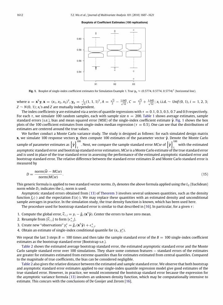
Fig. 1. Boxplot of single-index coefficient estimates for Simulation Example 1. True γ0 ≈ (0.5774, 0.5774, 0.5774)T (horizontal line).

where u = xTγ, x = (x1, x2, x3)T, γ0 =1√3(1, 1, 1)T, A =

√32 −

1.645√12, C =

√32 +

1.645√12; xi i.i.d. ∼ Unif (0, 1), i = 1, 2, 3;

Z ∼ N(0, 1); xi’s and Z are mutually independent.The index coefficients γ are estimated via a series of quantile regressions with τ = 0.1, 0.3, 0.5, 0.7 and 0.9 respectively.

For each τ , we simulate 100 random samples, each with sample size n = 200. Table 1 shows average estimates, samplestandard errors (s.e.), bias and mean squared error (MSE) of the single-index coefficient estimate γ. Fig. 1 shows the boxplots of the 100 coefficient estimates from single-index median regression (τ = 0.5). One can see that the distributions ofestimates are centered around the true values.We further conduct a Monte Carlo variance study. The study is designed as follows: for each simulated design matrix

x, we simulate 100 response vectors y, then compute 100 estimates of the parameter vector γ. Denote the Monte Carlo

sample of parameter estimates as{γ}1001. Next, we compare the sample standard errorMCse of

{γ}1001with the estimated

asymptotic standard error and bootstrap standard error estimators.MCse is aMonte Carlo estimate of the true standard errorand is used in place of the true standard error in assessing the performance of the estimated asymptotic standard error andbootstrap standard error. The relative difference between the standard error estimates se and Monte Carlo standard error ismeasured by

D =norm(se−MCse)norm(MCse)

. (15)

This generic formula is applied to two standard vector norms.D2 denotes the above formula applied using the L2 (Euclidean)norm while D1 indicates the L1 norm is used.Asymptotic standard errors obtained from (13) of Theorem 3 involves several unknown quantities, such as the density

function fy(·) and the expectation E(x|·). We may replace these quantities with an estimated density and unconditionalsample averages in practice. In the simulation study, the true density function is known, which has been used here.The procedure used for bootstrap standard error is similar to that described in [16]. In particular, for a given τ :

1. Compute the global error, ετ ,i = yi − gτ (xTγ). Center the errors to have zero mean.2. Resample from {ετ ,i} to form {ε∗τ ,i}.3. Create new ‘‘observations’’ y∗i = gτ (x

Tγ)+ ε∗τ ,i.4. Obtain an estimate of single-index conditional quantile for (xi, y∗i ).

We repeat the last 3 steps B = 100 times and then take the sample standard error of the B = 100 single-index coefficientestimates as the bootstrap standard error (Bootstrap s.e.).Table 2 shows the estimated average bootstrap standard error, the estimated asymptotic standard error and the Monte

Carlo sample standard error over 100 simulations. They share some common features — standard errors of the estimatesare greater for estimates estimated from extreme quantiles than for estimates estimated from central quantiles. Comparedto the magnitude of true coefficients, the bias can be considered negligible.Table 2 also gives the relative distance between the estimated and sample standard error.We observe that both bootstrap

and asymptotic standard error estimates applied to our single-index quantile regression model give good estimates of thetrue standard error. However, in practice, we would recommend the bootstrap standard error because the expression forthe asymptotic variance formula (13) involves an unknown density function, which may be computationally intensive toestimate. This concurs with the conclusions of De Gooijer and Zerom [16].


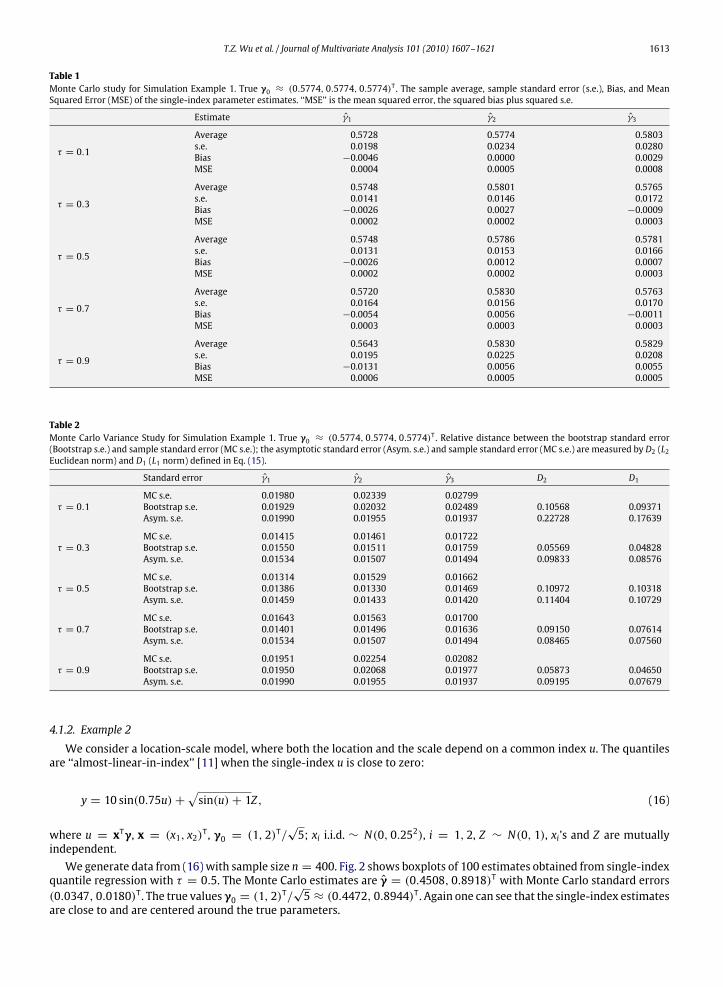
Table 1Monte Carlo study for Simulation Example 1. True γ0 ≈ (0.5774, 0.5774, 0.5774)T . The sample average, sample standard error (s.e.), Bias, and MeanSquared Error (MSE) of the single-index parameter estimates. ‘‘MSE’’ is the mean squared error, the squared bias plus squared s.e.

Estimate γ1 γ2 γ3

τ = 0.1

Average 0.5728 0.5774 0.5803s.e. 0.0198 0.0234 0.0280Bias −0.0046 0.0000 0.0029MSE 0.0004 0.0005 0.0008

τ = 0.3

Average 0.5748 0.5801 0.5765s.e. 0.0141 0.0146 0.0172Bias −0.0026 0.0027 −0.0009MSE 0.0002 0.0002 0.0003

τ = 0.5


τ = 0.7

Average 0.5720 0.5830 0.5763s.e. 0.0164 0.0156 0.0170Bias −0.0054 0.0056 −0.0011MSE 0.0003 0.0003 0.0003

τ = 0.9


Table 2Monte Carlo Variance Study for Simulation Example 1. True γ0 ≈ (0.5774, 0.5774, 0.5774)T . Relative distance between the bootstrap standard error(Bootstrap s.e.) and sample standard error (MC s.e.); the asymptotic standard error (Asym. s.e.) and sample standard error (MC s.e.) are measured by D2 (L2Euclidean norm) and D1 (L1 norm) defined in Eq. (15).

Standard error γ1 γ2 γ3 D2 D1

τ = 0.1MC s.e. 0.01980 0.02339 0.02799Bootstrap s.e. 0.01929 0.02032 0.02489 0.10568 0.09371Asym. s.e. 0.01990 0.01955 0.01937 0.22728 0.17639





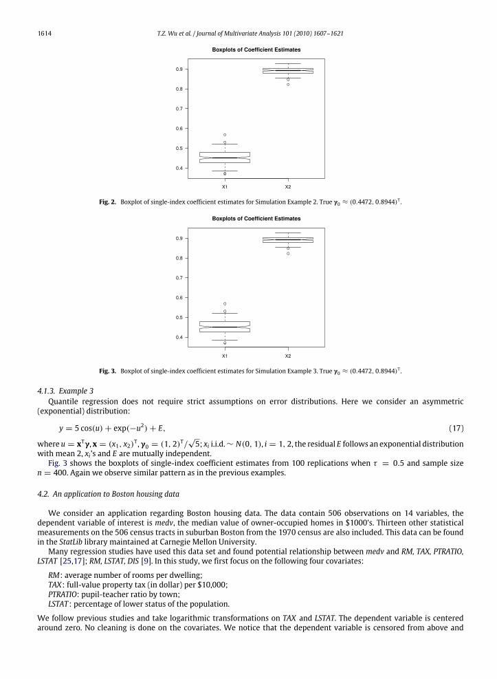
4.1.2. Example 2

We consider a location-scale model, where both the location and the scale depend on a common index u. The quantilesare ‘‘almost-linear-in-index’’ [11] when the single-index u is close to zero:

y = 10 sin(0.75u)+√sin(u)+ 1Z, (16)

where u = xTγ, x = (x1, x2)T, γ0 = (1, 2)T/√5; xi i.i.d. ∼ N(0, 0.252), i = 1, 2, Z ∼ N(0, 1), xi’s and Z are mutually

independent.We generate data from (16) with sample size n = 400. Fig. 2 shows boxplots of 100 estimates obtained from single-index

quantile regression with τ = 0.5. The Monte Carlo estimates are γ = (0.4508, 0.8918)T with Monte Carlo standard errors(0.0347, 0.0180)T. The true values γ0 = (1, 2)

T/√5 ≈ (0.4472, 0.8944)T. Again one can see that the single-index estimates

are close to and are centered around the true parameters.


Fig. 2. Boxplot of single-index coefficient estimates for Simulation Example 2. True γ0 ≈ (0.4472, 0.8944)T .

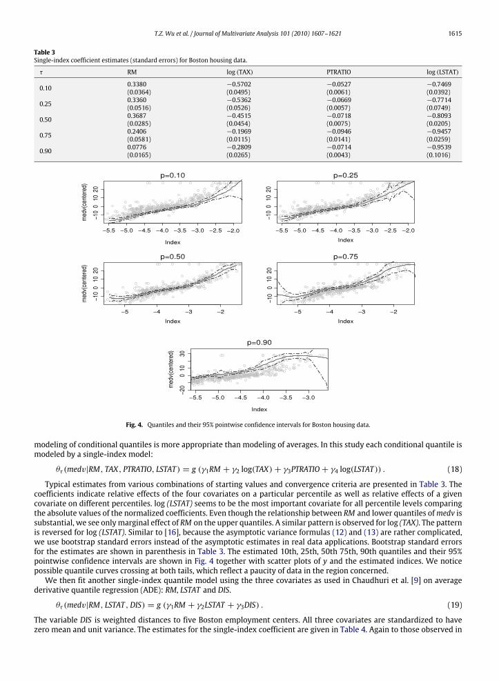
Fig. 3. Boxplot of single-index coefficient estimates for Simulation Example 3. True γ0 ≈ (0.4472, 0.8944)T .

4.1.3. Example 3Quantile regression does not require strict assumptions on error distributions. Here we consider an asymmetric

(exponential) distribution:

y = 5 cos(u)+ exp(−u2)+ E, (17)

where u = xTγ, x = (x1, x2)T,γ0 = (1, 2)T/√5; xi i.i.d.∼ N(0, 1), i = 1, 2, the residual E follows an exponential distribution

with mean 2, xi’s and E are mutually independent.Fig. 3 shows the boxplots of single-index coefficient estimates from 100 replications when τ = 0.5 and sample size

n = 400. Again we observe similar pattern as in the previous examples.

4.2. An application to Boston housing data

We consider an application regarding Boston housing data. The data contain 506 observations on 14 variables, thedependent variable of interest is medv, the median value of owner-occupied homes in $1000’s. Thirteen other statisticalmeasurements on the 506 census tracts in suburban Boston from the 1970 census are also included. This data can be foundin the StatLib library maintained at Carnegie Mellon University.Many regression studies have used this data set and found potential relationship between medv and RM, TAX, PTRATIO,

LSTAT [25,17]; RM, LSTAT, DIS [9]. In this study, we first focus on the following four covariates:

RM: average number of rooms per dwelling;TAX: full-value property tax (in dollar) per $10,000;PTRATIO: pupil-teacher ratio by town;LSTAT : percentage of lower status of the population.

We follow previous studies and take logarithmic transformations on TAX and LSTAT. The dependent variable is centeredaround zero. No cleaning is done on the covariates. We notice that the dependent variable is censored from above and


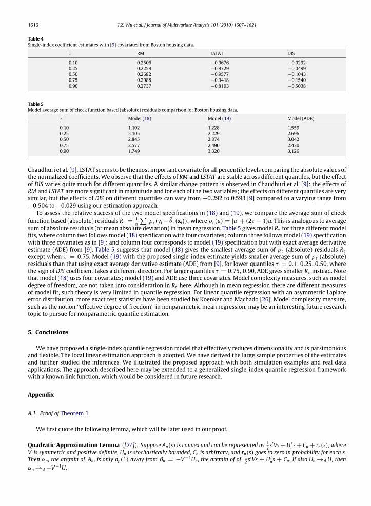
Table 3Single-index coefficient estimates (standard errors) for Boston housing data.

τ RM log (TAX) PTRATIO log (LSTAT)

0.10 0.3380 −0.5702 −0.0527 −0.7469(0.0364) (0.0495) (0.0061) (0.0392)

0.25 0.3360 −0.5362 −0.0669 −0.7714(0.0516) (0.0526) (0.0057) (0.0749)

0.50 0.3687 −0.4515 −0.0718 −0.8093(0.0285) (0.0454) (0.0075) (0.0205)

0.75 0.2406 −0.1969 −0.0946 −0.9457(0.0581) (0.0115) (0.0141) (0.0259)

0.90 0.0776 −0.2809 −0.0714 −0.9539(0.0165) (0.0265) (0.0043) (0.1016)

Fig. 4. Quantiles and their 95% pointwise confidence intervals for Boston housing data.

modeling of conditional quantiles is more appropriate than modeling of averages. In this study each conditional quantile ismodeled by a single-index model:

θτ (medv|RM, TAX, PTRATIO, LSTAT ) = g (γ1RM + γ2 log(TAX)+ γ3PTRATIO+ γ4 log(LSTAT )) . (18)

Typical estimates from various combinations of starting values and convergence criteria are presented in Table 3. Thecoefficients indicate relative effects of the four covariates on a particular percentile as well as relative effects of a givencovariate on different percentiles. log (LSTAT) seems to be the most important covariate for all percentile levels comparingthe absolute values of the normalized coefficients. Even though the relationship between RM and lower quantiles ofmedv issubstantial, we see onlymarginal effect of RM on the upper quantiles. A similar pattern is observed for log (TAX). The patternis reversed for log (LSTAT). Similar to [16], because the asymptotic variance formulas (12) and (13) are rather complicated,we use bootstrap standard errors instead of the asymptotic estimates in real data applications. Bootstrap standard errorsfor the estimates are shown in parenthesis in Table 3. The estimated 10th, 25th, 50th 75th, 90th quantiles and their 95%pointwise confidence intervals are shown in Fig. 4 together with scatter plots of y and the estimated indices. We noticepossible quantile curves crossing at both tails, which reflect a paucity of data in the region concerned.We then fit another single-index quantile model using the three covariates as used in Chaudhuri et al. [9] on average

derivative quantile regression (ADE): RM, LSTAT and DIS.

θτ (medv|RM, LSTAT ,DIS) = g (γ1RM + γ2LSTAT + γ3DIS) . (19)

The variable DIS is weighted distances to five Boston employment centers. All three covariates are standardized to havezero mean and unit variance. The estimates for the single-index coefficient are given in Table 4. Again to those observed in


Table 4Single-index coefficient estimates with [9] covariates from Boston housing data.

τ RM LSTAT DIS

0.10 0.2506 −0.9676 −0.02920.25 0.2259 −0.9729 −0.04990.50 0.2682 −0.9577 −0.10430.75 0.2988 −0.9418 −0.15400.90 0.2737 −0.8193 −0.5038

Table 5Model average sum of check function based (absolute) residuals comparison for Boston housing data.

τ Model (18) Model (19) Model (ADE)

0.10 1.102 1.228 1.5590.25 2.105 2.229 2.6960.50 2.845 2.874 3.0420.75 2.577 2.490 2.4300.90 1.749 3.320 3.126

Chaudhuri et al. [9], LSTAT seems to be themost important covariate for all percentile levels comparing the absolute values ofthe normalized coefficients. We observe that the effects of RM and LSTAT are stable across different quantiles, but the effectof DIS varies quite much for different quantiles. A similar change pattern is observed in Chaudhuri et al. [9]: the effects ofRM and LSTAT aremore significant inmagnitude and for each of the two variables; the effects on different quantiles are verysimilar, but the effects of DIS on different quantiles can vary from −0.292 to 0.593 [9] compared to a varying range from−0.504 to−0.029 using our estimation approach.To assess the relative success of the two model specifications in (18) and (19), we compare the average sum of check

function based (absolute) residuals Rτ = 1n

∑i ρτ (yi− θτ (xi)),where ρτ (u) = |u| + (2τ − 1)u. This is analogous to average

sum of absolute residuals (or mean absolute deviation) in mean regression. Table 5 gives model Rτ for three different modelfits, where column two followsmodel (18) specificationwith four covariates; column three followsmodel (19) specificationwith three covariates as in [9]; and column four corresponds to model (19) specification but with exact average derivativeestimate (ADE) from [9]. Table 5 suggests that model (18) gives the smallest average sum of ρτ (absolute) residuals Rτexcept when τ = 0.75. Model (19) with the proposed single-index estimate yields smaller average sum of ρτ (absolute)residuals than that using exact average derivative estimate (ADE) from [9], for lower quantiles τ = 0.1, 0.25, 0.50, wherethe sign of DIS coefficient takes a different direction. For larger quantiles τ = 0.75, 0.90, ADE gives smaller Rτ instead. Notethat model (18) uses four covariates; model (19) and ADE use three covariates. Model complexity measures, such as modeldegree of freedom, are not taken into consideration in Rτ here. Although in mean regression there are different measuresof model fit, such theory is very limited in quantile regression. For linear quantile regression with an asymmetric Laplaceerror distribution, more exact test statistics have been studied by Koenker and Machado [26]. Model complexity measure,such as the notion ‘‘effective degree of freedom’’ in nonparametric mean regression, may be an interesting future researchtopic to pursue for nonparametric quantile estimation.

5. Conclusions

We have proposed a single-index quantile regression model that effectively reduces dimensionality and is parsimoniousand flexible. The local linear estimation approach is adopted. We have derived the large sample properties of the estimatesand further studied the inferences. We illustrated the proposed approach with both simulation examples and real dataapplications. The approach described here may be extended to a generalized single-index quantile regression frameworkwith a known link function, which would be considered in future research.

Appendix

A.1. Proof of Theorem 1

We first quote the following lemma, which will be later used in our proof.

Quadratic Approximation Lemma ([27]). Suppose An(s) is convex and can be represented as 12 s′Vs+U ′ns+ Cn+ rn(s), where

V is symmetric and positive definite, Un is stochastically bounded, Cn is arbitrary, and rn(s) goes to zero in probability for each s.Then αn, the argmin of An, is only op(1) away from βn = −V−1Un, the argmin of of 12 s

′Vs + U ′ns + Cn. If also Un→d U, thenαn→d−V−1U.


We explicitly write g(u; h, γ) := g(u; γ) to indicate the dependence on h.

(nh)1/2{g(u; h, γ)− g0(u)} = (nh)1/2{g(u; h, γ)− g(u; h, γ0)} + (nh)1/2{g(u; h, γ0)− g0(u)}, (20)

where g(·; h, γ0) is a local linear estimator of g0(·) if the index coefficient γ0 is known. According to Theorem 3 in [23], wehave

(nh)1/2{g(u; h, γ0)− g0(u)− β(u)h2}D→ N

(0, α2(u)

). (21)

The first part on the right-hand side of (20), (nh)1/2{g(u; h, γ)− g(u; h, γ0)} can be shown op(1). The details are given below.For given u, for notational simplicity, we write aγ := g(u; h, γ), bγ := g ′(u; h, γ), aγ0 := g(u; h, γ0), and bγ0 :=

g ′(u; h, γ0)which are the solutions of the following minimization problems respectively,

mina,b

n∑i=1


i γ− u))K((xT

i γ− u)/h), (22)

mina,b

n∑i=1


i γ0 − u))K((xT

i γ0 − u)/h). (23)

We assume that the minimizers to both (22) and (23) exist for the following discussion to be meaningful and we want toshow whether (nh)1/2

(aγ − aγ0

)is op(1).

Each of the objective functions in (22) and (23) is non-differentiable and the resulting estimator is implicit. We considerquadratic approximation for each objective function. Under the root-n assumption on a preliminary estimator γ, we showquadratic approximations for (22) and (23) are ‘‘close enough’’ that their minimizers are ‘‘close enough’’ to each other in asense defined later.Denote

θ∗

n = (nh)1/2(aγ − g0(u), h(bγ − g ′0(u))

)T,

θ∗∗

n = (nh)1/2(aγ0 − g0(u), h(bγ0 − g

′

0(u)))T,

Z∗i =(1, (xT

i γ− u)/h)T, Z∗∗i =

(1, (xT

i γ0 − u)/h)T,

and denote

y∗i = yi − g0(u)− g′

0(u)(xTi γ− u), y∗∗i = yi − g0(u)− g

′

0(u)(xTi γ0 − u),

K ∗i = K((xTi γ− u)/h), K ∗∗i = K((x

Ti γ0 − u)/h).

Thus θ∗

n and θ∗∗

n minimize

Q ∗n (θ) =n∑i=1

[ρτ (y∗i − θTZ∗i /

√nh)− ρτ (y∗i )

]K ∗i and

Q ∗∗n (θ) =n∑i=1

[ρτ (y∗∗i − θTZ∗∗i /

√nh)− ρτ (y∗∗i )

]K ∗∗i respectively.

Both Q ∗n (θ) and Q∗∗n (θ) are convex in θ and they converge pointwise to their conditional expectations whose quadratic

approximations can be more easily derived. The convergence is also uniform on any compact set of θ [23]. Following [23],we can show in the same way

Q ∗n (θ) =12θTS∗θ+W∗n

Tθ+ r∗n (θ), r∗n (θ) = op(1), (24)

Q ∗∗n (θ) =12θTS∗∗θ+W∗∗n

Tθ+ r∗∗n (θ), r∗∗n (θ) = op(1), (25)

where

S∗ = S∗∗ = fU0(u)ϕ′′(0|u)

1 0

0∫

V

K(V)V2dV

,W∗n = −(nh)

−1/2∑

ρ ′τ (y∗

i )Z∗

i K∗

i , W∗∗n = −(nh)−1/2

∑ρ ′τ (y

∗∗

i )Z∗∗

i K∗∗

i .

Here ϕ′′(0|u) is the second derivative of ϕ(t|u) = E(ρτ (y− g0(u)+ t)|U = u)with respect to t evaluated at t = 0. The firstand second derivatives of ϕ(t|u)with respect to t , ϕ′(t|u) and ϕ′′(t|u), are assumed to exist. And V ∈ [−M,M], whereM issuch a real number that [−M,M] contains the support of K(·).


Write

Q ∗n (θ) = E(Q∗

n (θ)|X)− (nh)−1/2

(∑ρ ′τ (y

∗

i )Z∗

iTK ∗i − E(ρ

′

τ (y∗

i )|ui)Z∗

iTK ∗i

)θ+ R∗n(θ), (26)

where ρ ′τ (y∗

i ) only exists for y∗

i 6= 0, however we set ρ′τ (0) to 0 since y

∗

i = 0 occurs only with a probability of zero. Writeui = xT

i γ. Then we have the following result,

E(Q ∗n (θ)|X) = [ϕ(g0(ui)− g0(u)− g′

0(u)(ui − u)− θTZ∗i /√nh|ui)− ϕ(g0(ui)− g0(u)− g ′0(u)(ui − u)|ui)]K

∗

i

= −(nh)−1/2∑

ϕ′(g0(ui)− g0(u)− g ′0(u)(ui − u)|ui)(θTZ∗i )K

∗

i

+ (2nh)−1θT(∑

K ∗i ϕ′′(g0(ui)− g0(u)− g ′0(u)(ui − u)|ui)Z

∗

i Z∗

iT)

θ(1+ op(1))

= −(nh)−1/2∑E(ρ ′τ (y

∗

i )|ui)(θTZ∗i )K

∗

i

+ (2nh)−1θT(∑

K ∗i ϕ′′(g0(ui)− g0(u)− g ′0(u)(ui − u)|ui)Z

∗

i Z∗

iT)

θ(1+ op(1)), (27)

and

K ∗i ϕ′′(g0(ui)− g0(u)− g ′0(u)(ui − u)|ui) = K

∗

i (ϕ′′(0+ Op(h2)|u))

= K ∗i (ϕ′′(0|u)+ Op(h2)). (28)

The last equality requires ϕ′′′(0|u) exists and is bounded. The second term in the last equality of (27) can be rewritten as

(nh)−1∑K ∗i ϕ

′′(g0(ui)− g0(u)− g ′0(u)(ui − u)|ui)Z∗

i Z∗

iT= (nh)−1

∑K ∗i(ϕ′′(0|u)+ Op(h2)

)Z∗i Z∗

iT

= (nh)−1∑K ∗i ϕ

′′(0|u)Z∗i Z∗

iT (1+ Op(h2))

= S(1+ Op(h2)

), (29)

where

S = (nh)−1∑K ∗i ϕ

′′(0|u)Z∗i Z∗

iT

=

(s0 s1s1 s2

),

with the matrix components sj = (nh)−1∑K((ui − u)/h)ϕ′′(0|u)((ui − u)/h)j, j = 0, 1, 2.

E(sj) = h−1ϕ′′(0|u)∫

U

K((U− u)/h)((U− u)/h)jfU(U)dU

= ϕ′′(0|u)∫

V

K(V)V jfU0(Vh+ u)dV(1+ o(1))

recall V ∈ [−M,M]; fU(·) = fU0(·)(1+ o(1)) by Assumption (ii),

where U = xTγ,U0 = xTγ0, fU(·) and fU0(·) are their densities respectively.

= fU0(u)ϕ′′(0|u)

[∫V

K(V)V jdV](1+ o(1))

= fU0(u)ϕ′′(0|u)cj(1+ o(1)), where cj =

∫V

K(V)V jdV; c0 = 1, c1 = 0 from Assumption (i).

One can verify var(sj) = o(1). Therefore

S = fU0(u)ϕ′′(0|u)

(1 00 c2

)+ op(1) := S∗ + op(1), where c2 =

∫V

K(V)V2dV. (30)

By (27)–(30), we have

E(Q ∗n (θ)|X) = −(nh)−1/2

∑E(ρ ′τ (y

∗

i )|ui)(θTZ∗i )K

∗

i +12θTS∗θ(1+ op(1)). (31)

For R∗n(θ) defined by (26), R∗n(θ) = op(1). To save space, we refer readers to [23] for similar idea of proof. Substitute (31)

into (26), we have

Q ∗n (θ) =12θTS∗θ+W∗n

Tθ+ r∗n (θ), (32)


whereW∗n = −(nh)−1/2∑ ρ ′τ (y

∗

i )Z∗

i K∗

i is stochastically bounded, and r∗n (θ) = op(1). We outline the proof for stochastic

boundedness ofW∗n . By change of variable and existence of∫K 2(V)V jdV, j = 0, 1, 2 in Assumption (i), for some c > 0,

E(W∗nW∗

nT) ≤ cE

((nh)−1

∑(ρ ′τ (y

∗

i ))2(K ∗i )

2Z∗i Z∗

iT)

= O(h−1E

((K ∗i )

2Z∗i Z∗

iT))= O(1), (33)

which also implies E(W∗n) = O(1) as a result of Jensen’s inequality. Bounded secondmoment implies thatW∗n is stochastically

bounded. The asymptotic normality of θ∗

n = −S∗−1W∗ follows from that of W∗n as a result of Quadratic Approximation

Lemma. Eq. (25) can be shown similarly with S∗∗ = S∗,W∗∗n = −(nh)−1/2∑ ρ ′τ (y

∗∗

i )Z∗∗

i K∗∗

i , and r∗∗n (θ) = op(1).

According to the Quadratic Approximation Lemma, θ∗

n − θ∗

n = op(1) and θ∗∗

n − θ∗∗

n = op(1), where θ∗

n = −S∗−1W∗n and

θ∗∗

n = −S∗∗−1W∗∗n . Because of the root-n assumption on γ, we further show θ

∗

n − θ∗∗

n = op(1).Write S0 = S∗ = S∗∗,

θ∗

n − θ∗∗

n = −S−1(W∗n −W∗∗n )

= S−1(nh)−1/2∑

ρ ′τ (y∗

i )Z∗

i K∗

i − ρ′

τ (y∗∗

i )Z∗∗

i K∗∗

i

= S−1(nh)−1/2∑

ρ ′τ (y∗

i )(Z∗

i K∗

i − Z∗∗i K∗∗

i ).

The last equality is due to the fact that y∗∗i has the same sign as y∗

i a.s. when ‖γ− γ0‖ = Op(n−1/2). For some c > 0,

E((θ∗

n − θ∗∗

n )(θ∗

n − θ∗∗

n )T)≤ cS−1h−1E

((ρ ′τ (y

∗

i ))2(Z∗i K

∗

i − Z∗∗i K∗∗

i )(Z∗

i K∗

i − Z∗∗i K∗∗

i )T)(S−1)T,

= O(h−1E

((Z∗i K

∗

i − Z∗∗i K∗∗

i )(Z∗

i K∗

i − Z∗∗i K∗∗

i )T))= O (o(1)) = o(1), (34)

which also implies E(θ∗

n−θ∗∗

n ) = o(1). Thus, θ∗

n−θ∗∗

n = E(θ∗

n−θ∗∗

n )+op(1) = op(1) according to its first and secondmoment.Therefore θ

∗

n − θ∗∗

n = op(1). Take the first component of the vector, we obtain (nh)1/2{g(u; h, γ)− g(u; h, γ0)} = op(1).

Furthermore, when the bandwidth is taken at usual optimal rate, i.e. h ∈ Hn = {h : C1n−1/5 ≤ h ≤ C2n−1/5} [24], wehave (nh)1/2{g(u; h, γ)− g(u; h, γ0)} = op(1). That proves (nh)

1/2{g(u; h, γ)− g0(u)− β(u)h2}

D→ N(0, α2(u)). �


For given x,

(nh)1/2{θτ (x)− θτ (x)} = (nh)1/2{g(xTγ; γ)− g(xTγ0; γ)+ g(xTγ0; γ)− g0(x

Tγ0)}

= A+ (nh)1/2{g(xTγ0; γ)− g0(xTγ0)},

by the Taylor theorem, A = (nh)1/2{g(xTγ; γ) − g(xTγ0; γ)} = (nh)1/2g ′(xTγ0; γ)Op(‖γ − γ0‖) = op(n1/2h5/2), which is

op(1)when the bandwidth is taken at usual optimal rate. Then Theorem 2 is a result of of Theorem 1. �


We outline our approach to show asymptotic normality of γ. The proof will again rely on quadratic approximation andliterally follow a similar logic as in the proof of Theorem 2. Given (aj, bj), minimize the following to obtain γ,

n∑j=1

n∑i=1

ρτ

(yi − aj − bj(xi − xj)Tγ

)ωij. (35)

Write γ∗=√n(γ− γ0), then γ

∗ minimizes the following,

Qn(γ∗) =

n∑j=1

n∑i=1

[ρτ

(yij −

1√nbjxTijγ∗

)− ρτ (yij)

]ωij, (36)

where yij = yi − aj − bjxTijγ0. It can be shown that Qn(γ

∗) = 12γ∗TTnγ∗ + VT

nγ∗+ op(1), where Tn = 2C1, Vn =

(4τ(1− τ))1/2C01/2Zn, Zn→D N(0, I), and, C0 and C1 are defined in Assumption (v). In fact,

Qn(γ∗) = E(Qn(γ∗))−

1√n

n∑j=1

n∑i=1

[ωijρ

′

τ (yij)bjxTij − ωijE(ρ

′

τ (yij))bjxTij

]γ∗ +R(γ∗),

whereR(γ∗) = op(1).


Write ϕ(t|·) = ϕ(t|xTγ0 = xTγ0) = E(ρτ (y− θτ (x)+ t)|xTγ0 = x

Tγ0), we have

E(Qn(γ∗)) =n∑j=1

n∑i=1

[Eρτ

(yij −

1√nbjxTijγ∗

)− Eρτ (yij)

]ωij

=

n∑j=1

n∑i=1

Eρτ

(yij −

1√nbjxTijγ∗+1√nbjxTij(γ∗− γ∗)

)ωij

−

n∑j=1

n∑i=1

Eρτ

(yij −

1√nbjxTijγ∗+1√nbjxTijγ∗

)ωij

=

n∑j=1

n∑i=1

Eρτ

(yi − aj − bjxT

ijγ+1√nbjxTij(γ∗− γ∗)

)ωij

−

n∑j=1

n∑i=1

Eρτ

(yi − aj − bjxT

ijγ+1√nbjxTijγ∗

)ωij

=

n∑j=1

n∑i=1

Eρτ

(yi − g(xT

i γ|xTγ0 = x

Tγ0)+1√nbjxTij(γ∗− γ∗)

)ωij

−

n∑j=1

n∑i=1

Eρτ

(yi − g(xT

i γ|xTγ0 = x

Tγ0)+1√nbjxTijγ∗

)ωij

=

n∑j=1

n∑i=1

{ϕ

(1√nbjxTij(γ∗− γ∗)|xTγ0 = x

Tγ0

)− ϕ

(1√nbjxTijγ∗|xTγ0 = x

Tγ0

)}(1+ op(1))ωij.

By the Taylor expansion, we have

E(Qn(γ∗)) = −n∑j=1

n∑i=1

{ϕ′(1√nbjxTijγ∗|xTγ0 = x

Tγ0

)·1√nbjxTijγ∗

}(1+ op(1))ωij

+

n∑j=1

n∑i=1

{12n

γ∗T

[ϕ′′(1√nbjxTijγ∗|xTγ0 = x

Tγ0

)b2j xijx

Tij

]γ∗}(1+ op(1))ωij

= −1√n

n∑j=1

n∑i=1

{ϕ′(0|xTγ0 = x

Tγ0)bjxTijωij(1+ op(1))

}γ∗

+12n

γ∗Tn∑j=1

n∑i=1

{ϕ′′(0|xTγ0 = x

Tγ0)b2j xijx

Tijωij(1+ op(1))

}γ∗.

The last equation holds because of root-n assumption. Some simple calculation shows ϕ′(0|·) = 2(τ − Fy(g(xTi γ|·)))

and ϕ′′(0|) = 2fy(g(xTi γ|·)), where Fy(·) is the CDF and fy(·) is the p.d.f. On the other hand, for each Eρ

′τ (yij), Eρ

′τ (yij) =

2τ(1− Fyij(yij))+ 2(τ − 1)Fyij(yij) = 2(τ − Fyij(yij)). So we have the following representation,

Qn(γ∗) = −

1√n

[n∑j=1

n∑i=1

ρ ′τ (yij)bjxTijωij

]γ∗ +

12n

γ∗T

[n∑j=1

n∑i=1

2fy(.)(b2j xijxTij)ωij

]γ∗ + op(1).

Due to root-n consistency assumption, we have ρ ′τ (yij) given aj, bj has asymptotic distribution of ρ′τ (y− θτ (x)), i.e. equal to

2τ with a probability of 1− τ , and equal to 2(τ − 1)with a probability of τ , and has asymptotic mean of zero and varianceof 4τ(1− τ). Thus under Assumption (v), we have the following approximation,Qn(γ∗) = 1

2γ∗TTnγ∗+VT

nγ∗+op(1), where

Tn = 2C1, Vn = (4τ(1 − τ))1/2C01/2(Zn) and Zn→D N(0, I). Finally, by Quadratic Approximation Lemma and Slutsky’sTheorem, we have Theorem 3. Note that C1 is not positive definite due to norm 1 identifiability constraint. Generalizedinverse of C1 is used instead. The proof of the Quadratic Approximation Lemma indicates that the positive definiteness ofthe matrix can be reduced into semi-positive definiteness, even to the existence of a generalized inverse. �

References

[1] W. Lin, K.B. Kulasekera, Indentifiability of single-index models and additive-index models, Biometrica 94 (2007) 496–501.[2] R. Koenker, G.S. Bassett, Regression quantiles, Econometrica 46 (1978) 33–50.[3] H. Ichimura, Semiparametric Least Squares (SLS) and weighted SLS estimation of single-index models, Journal of Econometrics 58 (1993) 71–120.


[4] J.L. Horowitz, W. Härdle, Direct semiparametric estimation of single-index models with discrete covariates, Journal of the American StatisticalAssociation 91 (1996) 1623–1629.

[5] J.L. Horowitz, Semiparametric Methods in Econometrics, Springer, New York, 1998.[6] R.J. Carroll, J. Fan, I. Gijbels, M.P. Wand, Generalized partially linear single-index models, Journal of the American Statistical Association 92 (1997)477–489.

[7] Y. Yu, D. Ruppert, Penalized spline estimation for partially linear single-index models, Journal of the American Statistical Association 97 (2002)1042–1054.

[8] Y. Xia, W. Härdle, Semi-parametric estimation of partially linear single index models, Journal of Multivariate Analysis 97 (2006) 1162–1184.[9] P. Chaudhuri, K. Doksum, A. Samarov, On average derivative quantile regression, Annals of Statistics 25 (1997) 715–744.[10] E. Kong, Y. Xia, Quantile estimation of a general single-index model, Working paper, 2010. http://arxiv.org/abs/0803.2474.[11] K. Yu, M.C. Jones, Local linear quantile regression, Journal of the American Statistical Association 93 (1998) 228–237.[12] R. Koenker, P. Ng, S. Portnoys, Quantile smoothing splines, Biometrika 81 (1994) 673–680.[13] R. Koenker, Quantile Regression, Cambridge University Press, 2005.[14] C.J. Stone, Consistent nonparametric regression, with discussion, Annals of Statistics 5 (1977) 595–645.[15] P. Chaudhuri, Nonparametric estimates of regression quantiles and their local bahadur representation, Annals of Statistics 19 (1991) 760–777.[16] J.G. DeGooijer, D. Zerom, On additive conditional quantileswith high-dimensional covariates, Journal of the American Statistical Association 98 (2003)

135–146.[17] K. Yu, Z. Lu, Local linear additive quantile regression, Scandinavian Journal of Statistics 31 (2004) 333–346.[18] J.L. Horowitz, S. Lee, Nonparametric estimation of an additive quantile regression model, Journal of the American Statistical Association 100 (2005)

1238–1249.[19] W. Härdle, T.M. Stoker, Investing smooth multiple regression by the method of average derivatives, Journal of the American Statistical Association 84

(1989) 986–995.[20] K. Yu, M.C. Jones, A comparison of local constant and local linear regression quantile estimation, Computational Statistics and Data Analysis 25 (1997)

159–166.[21] Y. Xia, H. Tong, W.K. Li, L. Zhu, An adaptive estimation of dimension reduction space (with discussion), Journal of the Royal Statistical Society Series

B 64 (2002) 363–410.[22] D. Ruppert, S.J. Sheather, M.P. Wand, An effective bandwidth selector for local least squares regression, Journal of the American Statistical Association

90 (1995) 1257–1270.[23] J. Fan, T.C. Hu, Y.K. Truong, Robust nonparametric function estimation, Scandinavian Journal of Statistics 21 (1994) 433–446.[24] W. Härdle, P. Hall, H. Ichimura, Optimal smoothing in single-index models, Annals of Statistics 21 (1993) 157–178.[25] J.D. Opsomer, D. Ruppert, A fully automated bandwidth selection for additive regression model, Journal of the American Statistical Association 93

(1998) 605–618.[26] R. Koenker, J. Machado, Goodness of fit and related inference processes for quantile regression, Journal of the American Statistical Association 94

(1999) 1296–1310.[27] N.L. Hjort, D. Pollard, Asymptotics for minimisers of convex processes, 1993, Preprint.

http://arxiv.org/abs/0803.2474

Single-index quantile regression

Documents

Transcript of Single-index quantile regression