1

Chapter 13: Multiple Regression 13.1 Developing the multiple-Regression Model

The general model can be described as:

It simplifies for two independent variables:

The sample fit parameter b0, b1, and b2 are used to estimate the population parameter β0, β1, and β2 using the following regression equation:

2

Using Data Analysis - Regression for the first 3 columns of Potato.xls:

The fit equation allows us now to predict estimated values for the different experimental conditions. For example pH 4 and pressure 15 leads to:

984.10152805.047437.28162.3^

=∗−∗+=iY Our textbook now refers to Minitab for information about a confidence interval estimate of the average as well as a prediction interval estimate for a future individual value. The coefficient of Multiple Determination (R2)

4158.0977.995697.412

12. ===SSTSSRRY

This essentially means that 41.58% of the variation can be explained by the effect of pH and pressure on the solid content. The remaining 58.42% is due to random scattering of the data. Sometimes an adjusted R2 is suggested, which takes the number of data points (n) and the number of ‘explanatory’ variables (k = 2) into account.

( ) ( ) 3929.01254

1544158.0111

111 212.

2 =⎥⎦⎤

⎢⎣⎡

−−−

−−=⎥⎦⎤

⎢⎣⎡

−−−

−−=kn

nRR Yadj

3

13.2 Residual Analysis By plotting the difference between the actual data point value and the predicted value (residual), one can check the data for possible trends. The residuals are plotted against the various parameters, X1 and X2, as well as against the data point values, Y, or the time.

13.3 Testing of Significance of the Multiple Regression Model Essentially testing: H0: β1 = β2 = 0 (is there a slope with respect to any of the parameters?)

( )∑=

−=n

ii YYSST

1

2 ( )∑

=

−=n

ii YYSSR

1

2ˆ ( )∑=

−=n

iii YYSSE

1

2ˆ

13.4 Confidence Interval Estimate for each Slope The ‘standard error’ for each regression coefficient is provided in the PhStat analysis. Testing for the significance of each (slope) regression coefficient is:

or the Confidence Interval Estimate for the slope is:

jbknj stb 1−−±

4

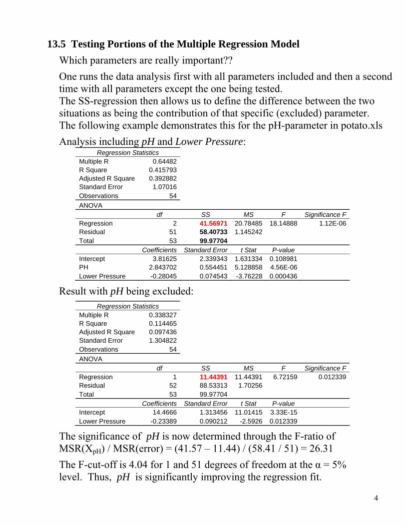
13.5 Testing Portions of the Multiple Regression Model Which parameters are really important?? One runs the data analysis first with all parameters included and then a second time with all parameters except the one being tested. The SS-regression then allows us to define the difference between the two situations as being the contribution of that specific (excluded) parameter. The following example demonstrates this for the pH-parameter in potato.xls Analysis including pH and Lower Pressure:

Regression Statistics Multiple R 0.64482 R Square 0.415793 Adjusted R Square 0.392882 Standard Error 1.07016 Observations 54 ANOVA

df SS MS F Significance F Regression 2 41.56971 20.78485 18.14888 1.12E-06Residual 51 58.40733 1.145242 Total 53 99.97704

Coefficients Standard Error t Stat P-value Intercept 3.81625 2.339343 1.631334 0.108981 PH 2.843702 0.554451 5.128858 4.56E-06 Lower Pressure -0.28045 0.074543 -3.76228 0.000436

Result with pH being excluded: Regression Statistics

Multiple R 0.338327 R Square 0.114465 Adjusted R Square 0.097436 Standard Error 1.304822 Observations 54 ANOVA

df SS MS F Significance F Regression 1 11.44391 11.44391 6.72159 0.012339Residual 52 88.53313 1.70256 Total 53 99.97704

Coefficients Standard Error t Stat P-value Intercept 14.4666 1.313456 11.01415 3.33E-15 Lower Pressure -0.23389 0.090212 -2.5926 0.012339

The significance of pH is now determined through the F-ratio of MSR(XpH) / MSR(error) = (41.57 – 11.44) / (58.41 / 51) = 26.31 The F-cut-off is 4.04 for 1 and 51 degrees of freedom at the α = 5% level. Thus, pH is significantly improving the regression fit.

5

Coefficient of Partial Determination Similar to the complete analysis of R2 as described in 13.1, one can also analyze how much variation in the data can be explained by a specific parameter as follows:

In our current example:

)(2172.02106.165697.41977.99

2106.16

)(3403.01258.305697.41977.99

1258.30

21.2

22.1

pressurelowerR

pHR

Y

Y

=+−

=

=+−

=

For a fixed lower pressure 34.03% of the variation can be explained by the variation in pH. And alternatively 21.72% of the variation can be explained by the variation of lower pressure.

6

13.6 The Quadratic Curvilinear Regression Model Essentially the testing procedure and interpretation of the results is the same as for the linear regression analysis. However, the second parameter now uses the square value of the first parameter. In a very similar way the regression models can be expanded to cubic or any other higher order relations.

The predicted Y-values are: 212110

ˆiii XbXbbY ++=

The significance of the Quadratic Curvilinear Model is given by the F-ratio between the mean square regression and the mean square error. F = MSR / MSE

As well as the “Coefficient of Multiple Determination”: R2Y.12 = SSR / SST

Estimation intervals for individual regression coefficients are described using the t-test with t = b2 / sb2 sb2 being the ‘standard error of the corresponding parameter in the Excel data analysis output. Details about the calculation of the standard error of a parameter are outside the scope of this class, but the systematic calculation is described on page 417 in Applied Statistics and Probability for Engineers, 3rd edition by Montgomery and Runger. The t-distribution is to be used for n – {# of fit-parameters} for the corresponding degrees of freedom. 13.7 Dummy-Variable Models Categorical variables can be substituted with ‘dummy variables’. For example, operator A is assigned a value of ‘0’ and operator B is assigned a value of ‘1’ (or ‘wet’ = 0 and ‘dry’ = 1). However, we should use this only in cases where the dummy variable has only two values. We can the further evaluate if the slope of the linear regression for our other parameters is affected by the dummy variable by adding an interaction factor.

7

13.8 Using Transformations in Regression Models

Similarly to what was already described in section 13.6, we can use all other kinds of transformations and regression models. E.g.: Square root transformation

iiii XXY εβββ +++= 22110

Multiplicative model iiii XXY εβ ββ 21

210= transforms to iiii XXY εβββ lnlnlnlnln 22110 +++=

Exponential model i

XXi

iieY εβββ 22110 ++= transforms to iiii XXY εβββ lnln 22110 +++=

In short, we can use any possible mathematical relation as long as we can describe the model as a combination of linear factors. 13.9 Collinearity

Collinearity describes a situation, where factors are highly correlated. It then becomes difficult to separate the individual effects from the cross-correlated effects and the effectiveness of a specific model can highly fluctuate depending on which parameters are being included. One way to evaluate collinearity is to use the variance inflationary factor:

2j 11VIF

jR−= with R2

j being the coefficient of determination when using

all other X-variables except Xj. Values close to 1 indicate ‘uncorrelated’ variables, whereas values of 5 or higher are considered significant. In other words, a large VIF value indicates that two (or more) variables are actually closely related. The two variables are not independent of each other but they are rather two measurements of the same effect. For example, measuring the bouncing height of a ball and correlating that to the speed of a falling ball 5 cm before hitting the ground (variable 1) and the height of where the ball was released initially (variable 2) are highly correlated variables. There is no need to include both variables in a model.

8

13.10 Model Building We like to achieve a ‘model’ that includes the fewest number of variables.

9

First we eliminate highly correlated variables. We then could use various combinations of variables and see if all of them show significance above a certain threshold in our regression model. In a more systematic way, we can use all possible combination of variables. The following figure shows the result for the potato-processing data.

We can now evaluate the adjusted R2 values of the different models. The larger the R2 value is, the more of the data scattering is being explained by the model. An alternative approach use the so-called Cp statistic for evaluation if a certain model should be considered. Here models where Cp is less than the number of variables being used in the model + 1 are being considered for further evaluation. Thereafter we again evaluate each model in detail and see if all variables show a significant effect (P-values below a given cut-off value). Nevertheless, choosing an appropriate model is a highly subjective process!

10

13.11 Pitfalls in Multiple Regression

The regression coefficient for one particular variable is interpreted for the case that all other variables are held constant.

We need residual plots for each independent variable.

Interaction plots are needed for each parameter when using dummy variables.

VIF evaluation is needed to decide on parameters to be included in a model.

Examine several alternative subsets for models.

Sample size 10 x larger than the # of variables in the model.

Evaluate a sufficiently wide range for each variable.

Stability over time is a key necessity to use a fitting model for predictive purposes.