Simple linear regression analysis

Workshop on Analysis of Clinical Studies – Can Tho University of Medicine and Pharmacy – April 2012

Simple linear regression

analysis

Tuan V. Nguyen

Professor and NHMRC Senior Research Fellow

Garvan Institute of Medical Research

University of New South Wales

Sydney, Australia


What we are going to learn …

• Examples

• Purposes of linear regression analysis

• Questions of interest

• Model parameters

• R analysis

• Interpretation


Femoral neck bone density and age

women = subset(vd, sex==2)

plot(fnbmd ~ age, pch=16)

abline(lm(fnbmd ~ age))

20 30 40 50 60 70 80

0.4

0.5

0.6

0.7

0.8

0.9

1.0

1.1

age

fnb

md


Weight and femoral neck bone density

plot(fnbmd ~ weight, pch=16)

abline(lm(fnbmd ~ weight))

30 40 50 60 70 80

0.4

0.5

0.6

0.7

0.8

0.9

1.0

1.1

weight

fnb

md


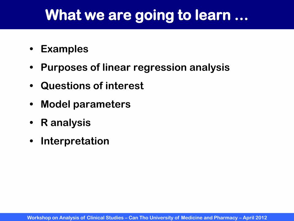
Correlation analysis

• Assessment of a relationship

• The coefficient of correlation: a measure of the

relationship

• We want to know more …

– The magnitude of effect of a predictor variable on the

outcome

– Prediction of outcome by using the predictor variable(s)


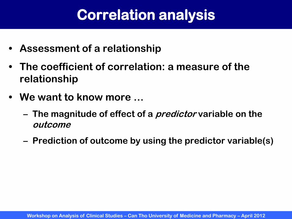
Our interests

• Finding a statistical model that decribes the

relationship between age, weight, and BMD

• Adjustment of effect

• Prediction

Linear regression model


Weight and femoral neck bone density

30 40 50 60 70 80

0.4

0.5

0.6

0.7

0.8

0.9

1.0

1.1

weight

fnb

md


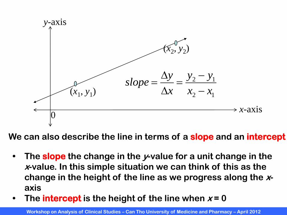
We can also describe the line in terms of a slope and an intercept

• The slope the change in the y-value for a unit change in the

x-value. In this simple situation we can think of this as the

change in the height of the line as we progress along the x-

axis

• The intercept is the height of the line when x = 0

(x1, y1)

(x2, y2)

x-axis

y-axis

2 1

2 1

y y yslope

x x x

0


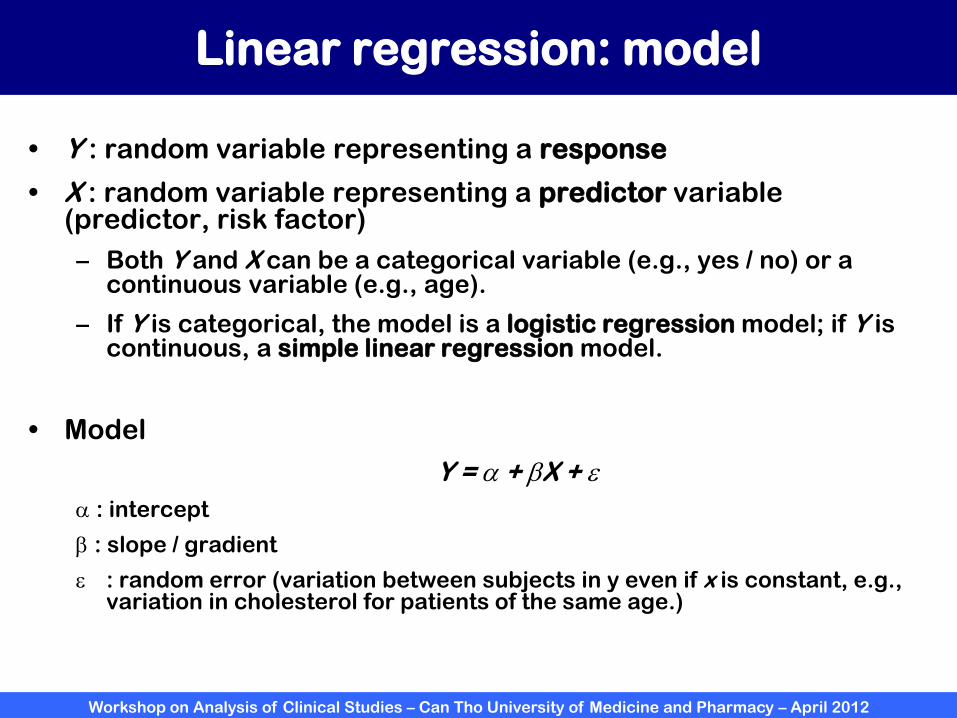
Linear regression: model

• Y : random variable representing a response

• X : random variable representing a predictor variable (predictor, risk factor)

– Both Y and X can be a categorical variable (e.g., yes / no) or a continuous variable (e.g., age).

– If Y is categorical, the model is a logistic regression model; if Y is continuous, a simple linear regression model.

• Model

Y = a + bX + e

a : intercept

b : slope / gradient

e : random error (variation between subjects in y even if x is constant, e.g., variation in cholesterol for patients of the same age.)


• The relationship is linear in terms of the parameter;

• X is measured without error;

• The values of Y are independently from each

other (e.g., Y1 is not correlated with Y2) ;

• The random error term (e) is normally

distributed with mean 0 and constant variance.

Linear regression: assumptions


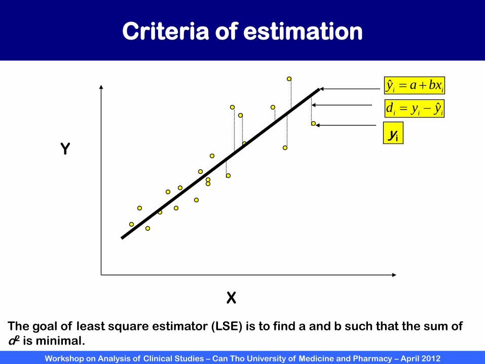
Criteria of estimation

Y

X

iibxay ˆ

iiiyyd ˆ

yi

The goal of least square estimator (LSE) is to find a and b such that the sum of

d2 is minimal.


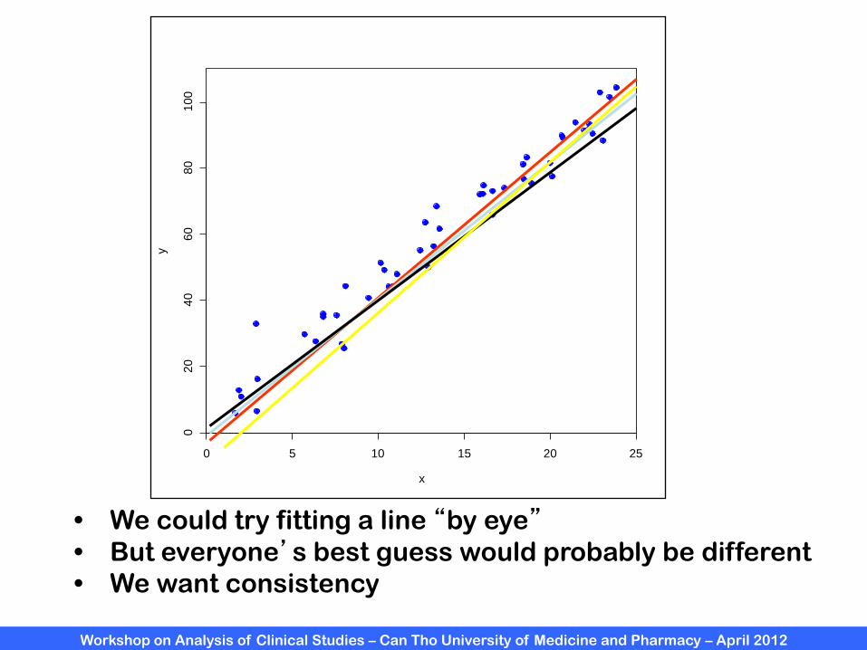
• We could try fitting a line “by eye”• But everyone’s best guess would probably be different

• We want consistency

0 5 10 15 20 25

02

04

06

08

01

00

x

y


Estimating parameters by R

• Our interest: relationship between BMD and weight

• Model:

BMD = a + b*weight + e

• We want to estimate a and b

• R language

lm(bmd ~ weight)


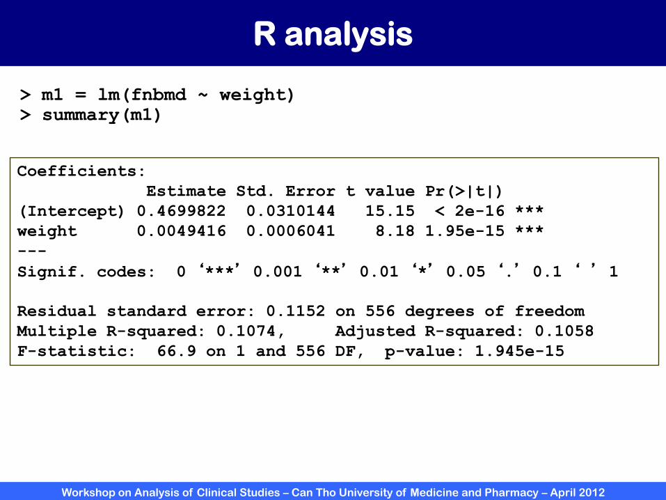
R analysis

> m1 = lm(fnbmd ~ weight)

> summary(m1)

Coefficients:

Estimate Std. Error t value Pr(>|t|)

(Intercept) 0.4699822 0.0310144 15.15 < 2e-16 ***

weight 0.0049416 0.0006041 8.18 1.95e-15 ***

---

Signif. codes: 0 ‘***’ 0.001 ‘**’ 0.01 ‘*’ 0.05 ‘.’ 0.1 ‘ ’ 1

Residual standard error: 0.1152 on 556 degrees of freedom

Multiple R-squared: 0.1074, Adjusted R-squared: 0.1058

F-statistic: 66.9 on 1 and 556 DF, p-value: 1.945e-15


Interpretation of outputs

Coefficients:

Estimate Std. Error t value Pr(>|t|)

(Intercept) 0.4699822 0.0310144 15.15 < 2e-16 ***

weight 0.0049416 0.0006041 8.18 1.95e-15 ***

• Remember our model:

BMD = a + b*weight

• Our equation:

BMD = 0.47 + 0.0049*weight

• Interpretation: 1 kg increase in weight was associated with a 0.0049 g/cm2 increase in BMD. The association is statistically significant (P < 0.0001)


BMD = 0.47 + 0.0049*weight

30 40 50 60 70 80

0.4

0.5

0.6

0.7

0.8

0.9

1.0

1.1

Weight

FN

BM

D


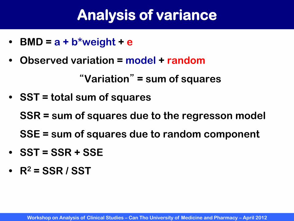
Analysis of variance

• BMD = a + b*weight + e

• Observed variation = model + random

“Variation” = sum of squares

• SST = total sum of squares

SSR = sum of squares due to the regresson model

SSE = sum of squares due to random component

• SST = SSR + SSE

• R2 = SSR / SST


Partitioning of variations: geometry

BMD

Weight

mean

SSR

SSE

SST

SST = SSR + SSE


Partitioning of variation by R

• Total SS = 0.8883 + 7.3819 = 8.2702

• R2 = 0.8883 / 8.2702 = 0.107


> anova(m1)

Analysis of Variance Table

Response: fnbmd

Df Sum Sq Mean Sq F value Pr(>F)

weight 1 0.8883 0.88829 66.905 1.945e-15 ***

Residuals 556 7.3819 0.01328

---

Signif. codes: 0 ‘***’ 0.001 ‘**’ 0.01 ‘*’ 0.05 ‘.’ 0.1 ‘ ’ 1


Interpretation of outputs

Residual standard error: 0.1152 on 556 degrees of freedom

Multiple R-squared: 0.1074, Adjusted R-squared: 0.1058

F-statistic: 66.9 on 1 and 556 DF, p-value: 1.945e-15

• R2 = 0.107

• Interpretation: Approximately 11% of BMD variance could be accounted for by body weight


Variance of BMD after adjusting for weight

• Mean square (MS) = sum of squares / (degrees of freedom)

• MS(residuals) = 7.3819 / 556 = 0.01328

Variance of BMD after adjusting for weight is 0.01328

(variance of BMD before the adjustment: 0.01485


> anove(m1)

Analysis of Variance Table

Response: fnbmd

Df Sum Sq Mean Sq F value Pr(>F)

weight 1 0.8883 0.88829 66.905 1.945e-15 ***

Residuals 556 7.3819 0.01328

---

Signif. codes: 0 ‘***’ 0.001 ‘**’ 0.01 ‘*’ 0.05 ‘.’ 0.1 ‘ ’ 1


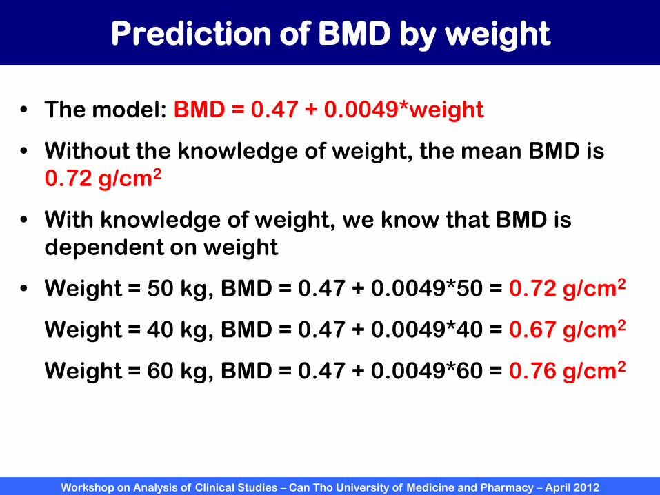
Prediction of BMD by weight

• The model: BMD = 0.47 + 0.0049*weight

• Without the knowledge of weight, the mean BMD is

0.72 g/cm2

• With knowledge of weight, we know that BMD is

dependent on weight

• Weight = 50 kg, BMD = 0.47 + 0.0049*50 = 0.72 g/cm2

Weight = 40 kg, BMD = 0.47 + 0.0049*40 = 0.67 g/cm2

Weight = 60 kg, BMD = 0.47 + 0.0049*60 = 0.76 g/cm2


Checking model assumptions

par(mfrow=c(2,2))

plot(m1)

0.65 0.75 0.85

-0.4

-0.2

0.0

0.2

0.4

Fitted values

Resid

uals

Residuals vs Fitted

3903

141

-3 -2 -1 0 1 2 3

-3-1

01

23

Theoretical Quantiles

Sta

ndard

ized r

esid

uals

Normal Q-Q

3903

141

0.65 0.75 0.85

0.0

0.5

1.0

1.5

Fitted values

Sta

ndard

ized r

esid

uals

Scale-Location390

3141

0.000 0.010 0.020 0.030

-3-1

12

3

Leverage

Sta

ndard

ized r

esid

uals

Cook's distance

Residuals vs Leverage

40

2713


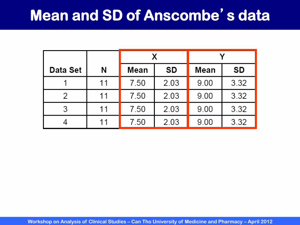
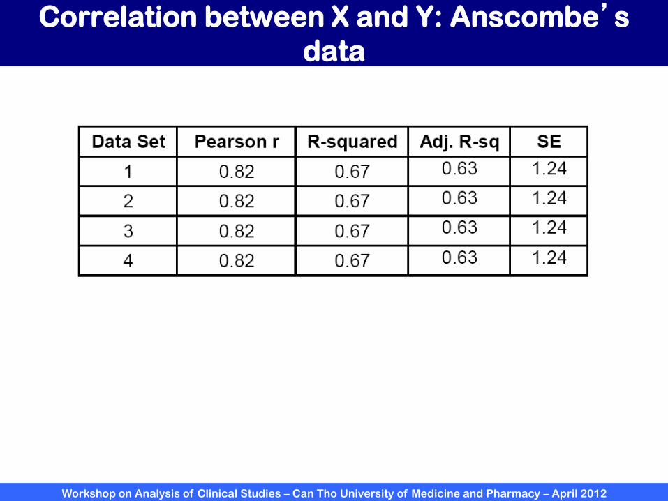
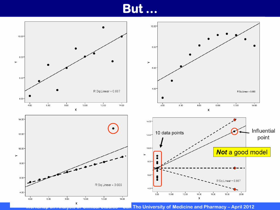
Be careful! Anscrombe’s data

Frank Anscombe devised 4 sets of X-Y pairs


Mean and SD of Anscombe’s data


Correlation between X and Y: Anscombe’s

data


Regression analysis: Anscombe’s data


But …


Summary

• Simple linear regression model is used for

– Understanding the effect of a risk factor or determinant

on an outcome variable

– Predicting an outcome variable

• It’s appropriate when the functional relationship is

linear

• Always check assumptions!

Simple linear regression analysis

Documents

Transcript of Simple linear regression analysis