Multiple Regression Methods

Hildebrand & Ott, Statistical Thinking for Manager, 4th edition, Chapter 121Hildebrand, Ott & Gray, Basic Statistical Ideas for Managers, 2nd edition, Chapter 12

Copyright © 2005 Brooks/Cole, a division of Thomson Learning, Inc.

Chapter 12:Multiple Regression Methods

Hildebrand, Ott and GrayBasic Statistical Ideas for Managers

Second Edition



Learning Objectives for Ch. 12

• The Multiple Linear Regression Model• How to interpret a slope coefficient in the multiple

regression model• The reason for using the adjusted coefficient of

determination in multiple regression• The meaning of multicollinearity and how to detect it• How to test the overall utility of the predictor• How to test the additional value of a single predictor• How to test the significance of a subset of predictors in

multiple regression• The meaning of extrapolation

2



Section 12.1The Multiple Regression Model



12.1 The Multiple Regression Model

Example (with two predictors):• Y = Sales revenue per region (tens of thousands of

dollars) • = advertising expenditures (thousands of dollars)• = median household income (thousands of dollars)

The data follow:

1x2x




• The data are:Region Sales Adv Exp Income

A 1 1 32B 1 2 38C 2 1 42D 2 3 35E 3 2 41F 3 4 43G 4 3 46H 4 5 44I 5 5 48J 5 6 45

• A graphical representation follows.




• Objective:

45

Sa les

1.040

2.5

4.0

Incom e

5.5

3524 306A dv Ex p

3 D S catte rp lot of S a le s v s Income v s Adv Ex p

Fit a plane through the points




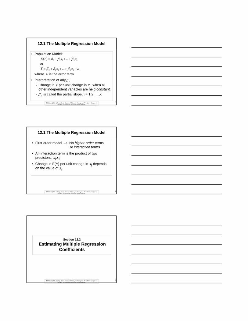
• Population Model:

or

where is the error term.

• Interpretation of any • Change in Y per unit change in , when all

other independent variables are held constant.• is called the partial slope, j = 1,2, …,k

kk xxYE βββ +++= ...)( 110

εβββ ++++= kk xxY ...110

εjβ

jx

jβ




• First-order model ⇒ No higher-order terms or interaction terms

• An interaction term is the product of two predictors:

• Change in E(Y) per unit change in depends on the value of .

1x2x

21xx



Section 12.2Estimating Multiple Regression

Coefficients



12.2 Estimating Multiple Regression Coefficients

• Criterion used to estimate β 'sMethod of Least Squares⇒ minimize the sum of squared residuals

• Symbolically: min

• We will use software to do the calculations

2

∑∧

−⎟⎟⎠

⎞

⎜⎜⎝

⎛ii yy




Example (Y = Sales, x1 = Advertising Expenditures, x2 = Median Household Income):

The Minitab output follows.Regression Analysis: Sales versus Adv Exp and Income

The regression equation isSales = - 5.09 + 0.416 Adv Exp + 0.163 Income

Predictor Coef SE Coef T P VIFConstant -5.091 1.720 -2.96 0.021Adv Exp 0.4158 0.1367 3.04 0.019 1.8Income 0.1633 0.0475 3.44 0.011 1.8

S = 0.541142 R-Sq = 89.8% R-Sq(adj) = 86.8%




• The fitted model is:

vs.

“The coefficient of an independent variable in a multiple regression equation does not, in general, equal the coefficient that would apply to that variable in a simple linear regression. In multiple regression, the coefficient refers to the effect of changing that variable while other independent variables stay constant. In simple linear regression, all other potential independent variables are ignored.” (Hildebrand, Ott and Gray)

1 25.09 0.416 0.163Y x x∧

= − + +

210.681 0.725 7.69 0.258Y = + x and Y = + x∧ ∧

−

jx

jx




• Interpretation of 0.416: An additional unit (or an increase of $1,000) of Advertising Expenditures leads to 0.416 increase in Sales when Median Household Income is fixed, i.e., regardless of whether is 32 or 48.

• Does this seem reasonable? • If Advertising Expenditures are increased by 1

unit, do you expect Sales to increase by 0.416 units regardless of whether the region has income of $32,000 or $48,000?

2x




• The output also gives the estimate of , both directly and indirectly.

• Indirectly, can be estimated as follows:

where = n - (k + 1) = n – k - 1

• The estimate of can also be read directly from “s” on the output.

εσ

εσ

Error)(Residual MS =

/df Residuals) Squaredof (Sum = sε

Errordf

εσ




Example (Sales vs. Adv. Exp. And Income): The Minitab output follows.Regression Analysis: Sales versus Adv Exp and Income


S = 0.541142 R-Sq = 89.8% R-Sq(adj) = 86.8%

Analysis of Variance

Source DF SS MS F PRegression 2 17.9502 8.9751 30.65 0.000Residual Error 7 2.0498 0.2928Total 9 20.0000




• Use the output to locate the estimate of

From the output, = 0.5411

Or,

εσ

εs

541.02928.0

)(

==

= ErrorMSsε




• Coefficient of Determination

• Concept: “…we define the coefficient of determination as the proportional reduction in the squared error of Y, which we obtain by knowing the values of .” (Hildebrand, Ott and Gray)

• As in simple regression,

⎟⎟⎠

⎞⎜⎜⎝

⎛•R or R 2

kxxxy

2

21

SSTSSE

- = SSTSSR

= R2 1

1 2, ,..., kx x x




Example (Sales vs. Adv. Exp. And Income):

From the output, “R-Sq = 89.8%”

Interpretation: 89.8% of the variation in Sales is explained by a multiple regression model with Adv. Exp. and Income as predictors.




• Adjusted Coefficient of Determination

• SSE and SST are each divided by their degrees of freedom.

• Since (n - 1) / (n - (k + 1)) > 1 ⇒

)( 2aR

) - (n / SST

)) + (k - (n / SSE - = Ra 1

112

SSTSSE

) + (k - n

- n - =

11

1

R <R 22a




• Why use ?

• SST is fixed, regardless of the number of predictors.

• SSE decreases when more predictors are used. ⇒ R2 increases when more predictors are used.

• However, can decrease when another predictor is added to the fitted model, even though R2

increases.

• Why? The decrease in SSE is offset by the loss of a degree of freedom in [n – (k +1)] for SSE.

2aR

2aR




• The following example illustrates this.

Example:For a fitted model with 10 observations, suppose SST = 50. When k = 2, SSE = 5. When k = 3, SSE = 4.5.

• Even though there has been a modest increase in , has decreased.

2R2

αR

2R 2αR

K=2:

K=3: 865.50

5.469191.

505.41

871.505

7919.

5051

=⎟⎠⎞

⎜⎝⎛

⎟⎠⎞

⎜⎝⎛−=−

=⎟⎠⎞

⎜⎝⎛

⎟⎠⎞

⎜⎝⎛−=−




• Sequential Sum of Squares (SEQ SS)• Concept: The incremental contributions to SS

(Regression) when the predictors enter the model in the order specified by the user.

Example (Sales vs. Adv. Exp. And Income):The Minitab output follows for when Adv.Exp. is entered first.

Analysis of VarianceSource DF SS MS F PRegression 2 17.9502 8.9751 30.65 0.000

Source DF Seq SSAdv Exp 1 14.4928Income 1 3.4574




• SS (Regression Using and )SSR ( , )

= 17.9502• SS (Regression Using only)

SSR ( ) = 14.4928

• SS (Regression for when is already in the model)

SSR ( | ) = 3.4574

1x 2x1x

1x

2x

2x 1x2x 1x

≡

≡ 1x

≡




Example (Sales vs. Adv. Exp. And Income):The Minitab output follows for when Income is entered first.

Analysis of VarianceSource DF SS MS F PRegression 2 17.9502 8.9751 30.65 0.000

Source DF Seq SSIncome 1 15.2408Adv Exp 1 2.7093




• SS (Regression Using and ) SSR ( , ) = 17.9502 {Unchanged

• SS (Regression Using only) SSR ( ) = 15.2408

• SS (Regression for when is already in the model)

SSR ( | ) = 2.7093

• Regardless of which predictor is entered first, the sequential sums of squares, when added, equal SS (Regression).

1x1x

1x

2x

2x2x

2x1x

≡

2x≡

≡

2x



Section 12.3Inferences in Multiple Regression



12.3 Inferences in Multiple Regression

• Objective: Build a parsimonious model⇒ as few predictors as necessary

• Must now assume errors in population model are normally distributed

• F-test for overall model

vs. 0...:H 210 === kβββ

0:Ha ≠joneleastat β




• Test Statistic: F = MS (Regression)/MS (Residual Error)

• Concept: “If SS (Regression) is large relative to SS (Residual), the indication is that there is real predictive value in [some of] the independent variables .”(Hildebrand, Ott and Gray)

• Decision Rule: Rejector reject α<− valuepifH0

1 2, ,..., kx x x

1,,0 −−> knkFFifH α




Example (Sales vs. Adv. Exp. and Income):

The Minitab output follows:

Analysis of VarianceSource DF SS MS F PRegression 2 17.9502 8.9751 30.65 0.000Residual Error 7 2.0498 0.2928Total 9 20.0000




Test : At least one

at the 5% level.

Since F = 30.65 > F.05, 2, 7 = 4.74,

reject at the 5% level.

Or since p-value = 0.000 < .05,


Implication: At least one of the x’s has some predictivepower.

aHvsH .0: 210 == ββ 0≠jβ

0: 210 == ββH

0: 210 == ββH




• t-test for Significance of an Individual Predictor

• implies that has no additional predictive value as the last predictor in to a model that contains all the other predictors

• Test Statistic: t =

where is the estimated standard error of

k , 1,2, j,0:.0:H0 …=≠= jaj Hvs ββ

0H jx

ˆˆ( 0) /

jj sβ

β −

ˆj

sβ

ˆjβ




• In Minitab notation, T = (Coef) / (SE Coef)

• Decision Rule: Reject

or reject if p-value < α.

• Warning: Limit the number of t-tests to avoida high overall Type 1 error rate.

1,2/0 −−> knttifH α

0H





The Minitab output follows:

Predictor Coef SE Coef T P VIFConstant -5.091 1.720 -2.96 0.021Adv Exp 0.4158 0.1367 3.04 0.019 1.8Income 0.1633 0.0475 3.44 0.011 1.8

Test at the 5% level.0:.0: 110 ≠= ββ aHvsH




Since


Or since p-value = .019 < .05,


Implication: Advertising Expenditures provides additional predictive value to a model having Income as a predictor

,365.204.3 7,025. =>= tt0: 10 =βH

0: 10 =βH




• MulticollinearityConcept: High correlation between at least one pair of

predictors, e.g., x1 and x2

⇒ Correlated x's provide no new information.Example: In predicting heights of adults using the length of

the right leg, the length of the left leg would be of little value.

• Symptoms of Multicollinearity• Wrong signs for s• t-test isn't significant even though you believe the

predictor is useful and should be in the fitted model.

β ′ˆ




• Detection of Multicollinearity

• is the coefficient of determination obtained by regressing xj on the remaining (k - 1) predictors, denoted by .

• If > 0.9, this is a signal that multicollinearity is present.

• This criterion can be expressed in a different way.

R2x x x x x k1 +j 1 -j 1j •••••••

2jR

2jR




• Let VIFj denote the Variance Inflation Factor of the jth predictor:

• If VIFj > 10, this is a signal that multicollinearity is present.

2

11j

j

VIFR

=−




• Why is VIFj called the variance inflation factor for the jth predictor?

• The estimated standard error of in a multiple regression is:

or

jβ∧

∑ −−=

)1()(1

22ˆjjij Rxx

ssj

εβ

∑ −= 2ˆ )( jij

j

xxVIF

ssj

εβ




• If VIFj is large, so is , which leads to a t-test

that is not statistically significant.

• The VIF “ …measures how much the variance (square of the standard error) of a coefficient is increased because of collinearity.” (Hildebrand, Ott and Gray)

j

sβ∧





The Minitab output follows. The regression equation isSales = - 5.09 + 0.416 Adv Exp + 0.163 IncomePredictor Coef SE Coef T P VIFConstant -5.091 1.720 -2.96 0.021Adv Exp 0.4158 0.1367 3.04 0.019 1.8Income 0.1633 0.0475 3.44 0.011 1.8

Since both VIFs = 1.8 < 10, multicollinearity between Advertising Expenditures and Median Household Income is not a problem.




• The Minitab output for regressing Adv Exp on Income follows:

The regression equation is

Adv Exp = - 6.26 + 0.229 Income

S = 1.39955 R-Sq = 43.2%

Since R2 =.432, VIF = 1/(1 - .432) = 1.8, as shown.




• To illustrate multicollinearity, consider Exercise 12.19• Exercise 12.19: A study of demand for imported

subcompact cars consists of data from 12 metropolitan areas. The variables are: Demand: Imported subcompact car sales as a

percentage of total salesEduc: Average number of years of schooling

completed by adultsIncome: Per capita incomePopn: Area populationFamsize: Average size of intact families




The Minitab output follows:The regression equation isDemand = - 1.3 + 5.55 Educ + 0.89 Income + 1.92 Popn

- 11.4 Famsize

Predictor Coef SE Coef T P VIFConstant -1.32 57.98 -0.02 0.982Educ 5.550 2.702 2.05 0.079 8.8Income 0.885 1.308 0.68 0.520 4.0Popn 1.925 1.371 1.40 0.203 1.6Famsize -11.389 6.669 -1.71 0.131 12.3

S = 2.68628 R-Sq = 96.2% R-Sq(adj) = 94.1%




• Is there a multicollinearity (MC) problem?

Since the VIF = 12.3 > 10 for the variable “Famsize”, there is a MC problem.

• Note that the p-value for the F test = 0.000, indicating that at least one of the x’s has predictive value. However, the smallest p-value for any t-test is 0.079, indicating that not one of the individual x’s has predictive value.

• What is the source of the MC problem?A matrix plot, in conjunction with the correlations, couldbe useful. This exercise will be revisited in Section 13.1




• Remedies if multicollinearity is a problem.

• Eliminate one or more of the collinear predictors.

• Form a new predictor that is a surrogate of collinear predictor

• Multicollinearity could occur if one of the predictors is .

• This can be eliminated by using as the predictor.

2( )x x−

2x



Section 12.4Testing a Subset of the Regression

Coefficients



12.4 Testing a Subset of the Regression Coefficients

• To illustrate the concept, consider Exercise 13.55Exercise 13.55: A bank that offers charge cards to customers

studies the yearly purchase amount (in thousands of dollars) on the card as related to the age, income (in thousands of dollars), whether the cardholder owns or rents a home and years of education of the cardholder. The variable owner equals 1 if the cardholder owns a home and 0 if the cardholder rents a home. The other variables are self-explanatory. The original data set has information on 160 cardholders. Upon further examination of the data, you decide to remove the data for cardholder 129 because this is an older individual who has a high income from having saved early in life and having invested successfully. This cardholder travels extensively and frequently uses her/his charge card.




Problem to be investigated:

The income and education predictors measure the economic well-being of a cardholder.

Do these predictors have any predictive value given the age and home ownership variables?

The null hypothesis is that the β’s corresponding to these predictors are simultaneously equal to 0.




• General Case

Complete Model:

Null hypothesis:

Reduced Model:

kkgggg xxxxYE βββββ ++++++= ++ …… 11110)(

gg xxYE βββ +++= …110)(

0: 10 ===+ kgH ββ …




• Exercise 13.55

Complete Model:

Null hypothesis:

Reduced Model:

)()()()()( 43210 EducnIncomeOwnerAgeYE βββββ ++++=

0:0 == EducnIncomeH ββ

)()()( 210 OwnerAgeYE βββ ++=




• The test statistic is called the Partial F statistic

Partial F Statistic

• Rationale• SSE decreases as new terms are added to the model. • If the x’s from (g + 1) to k have predictive ability, then

SSEcomplete should be much smaller than SSEreduced

• Their difference [SSEreduced – SSEcomplete] should be large

]/[][]/[][

completecomplete

completereducedcompletereduced

dfSSEdfdfSSESSE

F−−

=




Note: dfreduced - dfcomplete = k – g; dfcomplete = n – (k + 1)

Note: SSEcomplete/dfcomplete = MSEcomplete

Note: Other versions of the partial F-test are in H,O&G.

• Decision criterion: Reject H0 if Partial F > Fα,k-g,n-k-1




Exercise 13.55:

(from the Minitab output that follows)

Since 6.045 > F.05,2,154=3.055, reject H0.Either Income or Education add predictive value to

a model that contains Age and Owner

0:0 == EducnIncomeH ββ

045.60078.

]24/[]1937.1288.1[

]/[][]/[][

=−−

=

−−=

completecomplete

completereducedcompletereduced

dfSSEdfdfSSESSE

F




Regression Analysis: Purch_1 versus Age_1, Income_1, Owner_1, Educn_1

The regression equation isPurch_1 = - 0.797 + 0.0336 Age_1 + 0.00927 Income_1 +

0.112 Owner_1 + 0.00928 Educn_1

S = 0.08804 R-Sq = 95.0% R-Sq(adj) = 94.8%


Source DF SS MS F PRegression 4 22.4678 5.6170 724.62 0.000Residual Error 154 1.1937 0.0078Total 158 23.6616




Regression Analysis: PURCH_1 versus AGE_1, OWNER_1

The regression equation isPURCH_1 = - 0.602 + 0.0402 AGE_1 + 0.220 OWNER_1

S = 0.09085 R-Sq = 94.6% R-Sq(adj) = 94.5%


Source DF SS MS F P

Regression 2 22.374 11.187 1355.48 0.000

Residual Error 156 1.288 0.008

Total 158 23.662



Section 12.5Forecasting Using Multiple

Regression



12.5 Forecasting Using Multiple Regression

• A major purpose of regression is to make predictions using the fitted model.

• In simple regression, we could obtain a confidence interval for E(Y) or a prediction interval for an individual Y.

• In both cases, the danger of extrapolation must be considered.

• Extrapolation occurs when using values of x far outside the range of x-values used to build the fitted model.




• In regressing Sales on Advertising Expenditures, Advertising Expenditures ranged from 1 to 6.

It would be incorrect to obtain a Confidence Interval for E(Y) or a Prediction Interval for Y far outside this range.

We don’t know if the fitted model is valid outside this range.

• In multiple regression, one must consider not only the range of each predictor but the set of values of the predictors taken together.




• Consider the following example: Example:

Y = sales revenue per region (tens of thousands of dollars) x1 = advertising expenditures (thousands of dollars) x2 = median household income (thousands of dollars)

The values for x1 and x2 are:

45484446434135423832x2

6553423121x1

JIHGFEDCBARegion




• The scatterplot for x1 vs. x2 follows.




• Extrapolation occurs when using the fitted model to predict outside the elbow-shaped region.

• This would occur when Advertising Expenditures is 5 and income is 35.

• The Minitab output follows




Regression Analysis: Sales versus Adv Exp, Income


Predicted Values for New ObservationsNewObs Fit SE Fit 95% CI 95% PI1 2.703 0.530 (1.451, 3.956) (0.913, 4.494) XX denotes a point that is an outlier in the predictors.

Values of Predictors for New ObservationsNewObs Adv Exp Income1 5.00 35.0

Minitab indicates that this set of values for x1 and x2 is an outlier



Keywords: Chapter 12

• Multiple regression model

• Partial slopes• First order model• Adjusted Coefficient

of Determination, Ra2

• Multicollinearity• Variance Inflation

Factor

• Overall F test• t-test• Complete model• Reduced model• Partial F test• Extrapolation

63



Summary of Chapter 12

• The Multiple Linear Regression Model• Interpreting the slope coefficient of a single predictor in a

multiple regression model• Understanding the difference between the coefficient of

determination (Ra2) and the adjusted coefficient of

determination (R2)• The detection of multicollinearity and its impact• Using the F statistic to test the overall utility of the predictors• Using the t-test to test the additional value of a single

predictors• Using the partial F test for assessing the significance of a

subset of predictors• The meaning of extrapolation in multiple regression

64

Multiple Regression Methods

Documents

Transcript of Multiple Regression Methods