Using commonality analysis in multiple regressions:a tool to decompose regression effects in the...

Using commonality analysis inmultiple regressions: a

tool to decompose regression effects in the face of

multicollinearity

Jayanti Ray-Mukherjee1*, KimNimon2, ShomenMukherjee1, DouglasW.Morris3,

RobSlotow1 andMichelle Hamer1,4

1TheSchool of Life Sciences, University of KwaZulu-Natal,Westville Campus, Private Bag: X54001, Durban 4000, South

Africa; 2Learning Technologies andCollege of Information, University of North Texas, 3940N. Elm, RmG150Denton, TX,

76207, USA; 3Department of Biology, LakeheadUniversity, Thunder Bay, ON, P7B 5E1, Canada; and 4South AfricanNational

Biodiversity Institute, Private BagX101, Pretoria 0001, South Africa

Summary

1. In the face of natural complexities and multicollinearity, model selection and predictions using

multiple regression may be ambiguous and risky. Confounding effects of predictors often cloud

researchers’ assessment and interpretation of the single best ‘magicmodel’. The shortcomings of step-

wise regression have been extensively described in statistical literature, yet it is still widely used in eco-

logical literature. Similarly, hierarchical regression which is thought to be an improvement of the

stepwise procedure, fails to address multicollinearity.

2.We propose that regression commonality analysis (CA), a technique more commonly used in psy-

chology and education research will be helpful in interpreting the typical multiple regression analyses

conducted on ecological data.

3.CA decomposes the variance ofR2 into unique and common (or shared) variance (or effects) of pre-

dictors, and hence, it can significantly improve exploratory capabilities in studies where multiple

regressions are widely used, particularly when predictors are correlated. CA can explicitly identify

themagnitude and location ofmulticollinearity and suppression in a regressionmodel.

In this paper, using a simulated (from a correlation matrix) and an empirical dataset (human habitat

selection, migration of Canadians across cities), we demonstrate howCA can be used with correlated

predictors in multiple regression to improve our understanding and interpretation of data. We

strongly encourage the use of CA in ecological research as a follow-on analysis frommultiple regres-

sions.

Key-words: stepwise regression, hierarchical regression, structure coefficients, standardized partial

regression coefficient, suppressor variable, habitat selection

Introduction

Multiple linear regression (MR) is widely used to identifymod-

els that capture the essence of ecological systems (Whittingham

et al. 2006). MR extends simple linear regression to model the

relationship between a dependent variable (Y) and more than

one independent (also known as ‘predictor’ and so-called

henceforth) variables (Sokal &Rohlf 1995). Owing to the com-

plexity of ecological systems, multicollinearity among predic-

tor variables frequently poses serious problems for researchers

usingMR (Graham 2003).

Quite often, ecologists pose the question, to what extent is

variation in each predictor variable associated (linearly) with

variation in the dependent variable? To answer this, in MR,

there are three main effects that need to be assessed: (i) total

effects – total contribution of each predictor variable to the

regression when the variance of other predictors are accounted

for; (ii) direct effects –contribution of a predictor, independent

of all other predictors; and (iii) partial effects –contribution of

a predictor when accounting for variance of a specific subset or

subsets of remaining predictors (LeBreton, Ployhart & Ladd

2004). However, conventionally, one reports the coefficient of

determination (R2) and regression coefficients, where the

P-values of the regression coefficients are the information one

mostly relies upon to answer the fairy-tale question, ‘Mirror,

mirror on the wall, what is the best predictor of them all?’

(Nathans, Oswald&Nimon 2012; p. 1).

The R2 quantifies the extent to which the variance of the

dependent variable is explained by variance in the predictor*Correspondence author. E-mail: [email protected]

© 2014 The Authors. Methods in Ecology and Evolution © 2014 British Ecological Society

Methods in Ecology and Evolution 2014 doi: 10.1111/2041-210X.12166

set, and regression coefficients help rank the predictor vari-

ables according to their contributions in the regression equa-

tion (Nimon et al. 2008). However, relying only on the

unstandardized slope of regression (also known as partial

regression coefficients, Sokal & Rohlf 1995) or standardized

(partial) regression coefficients (also known as beta coefficients

and so-called henceforth, Sokal & Rohlf 1995) may generate

erroneous interpretations, particularly when multicollinearity

is involved (Courville & Thompson 2001; Kraha et al. 2012).

It is not uncommon for researchers to erroneously refer to beta

coefficients as measures of relationship between predictors and

the dependent variable (Courville & Thompson 2001). Hence,

it is often advisable to use multiple methods while interpreting

MR results, especially when the intentions are not strictly pre-

dictive (Nimon & Reio 2011). In this paper, we use simulated

and empirical data to demonstrate how a relatively similar

approach, regression commonality analysis (CA), can be used

along with beta coefficients and structure coefficients to better

interpretMR results in the face of multicollinearity.

Why are stepwise or hierarchical regressions notenough?

Complexities in most systems warrant that ecologists collect

data on variables of importance and of interest in concert with

data on factors that might affect a response (Whittingham

et al. 2006).When a researcher is interested in determining pre-

dictors’ contribution, MR is used to either choose predictor

variables based on statistics (stepwise regression) or identify

the predictor variables that support a theory (hierarchical

regression; Lewis 2007).

Stepwise regressions, which are widely used in ecological

studies, provide a methodology to determine a predictor vari-

able’s meaningfulness as it is introduced into a regression

model (Pedhazur 1997; Graham 2003). Though widely used in

fields such as animal behavior and species distribution model-

ling (Ara�ujo & Guisan 2006; Smith et al. 2009), stepwise

regression is often discouraged owing to its approach of ‘data

dredging’ and lack of theory (Burnham & Anderson 2002;

Whittingham et al. 2006). This procedure cause biases and

inconsistencies in parameter estimation, model selection algo-

rithms, selection order of different predictors and selection of

the single bestmagic model (seeWhittingham et al. 2006; Zien-

tek & Thompson 2006; Nathans, Oswald & Nimon 2012;

Suppl mat.). Stepwise regression relies largely on the first pre-

dictor entering the model, which determines the variance of

other predictors in the model, posing serious Type I errors

associated with inflated F-values (Thompson 1995; Zientek &

Thompson 2006; Nimon et al. 2008; Nathans, Oswald & Ni-

mon 2012). Hence, the use of stepwise regression has been dis-

couraged for assessing the contributions of predictor variables

inMR (Nathans, Oswald&Nimon 2012).

Hierarchical regression is more replicable and reliable for

evaluating the contribution of predictors and is thus an

improvement over stepwise regression (Thompson 1995;

Pedhazur 1997; Lewis 2007). Rather than using the familiar

stepwise procedure, the choice and order of variables in hierar-

chical regression is based on a priori knowledge of theory

(Thompson 1995; Pedhazur 1997; Lewis 2007; Nathans,

Oswald & Nimon 2012) that help researchers to more effec-

tively choose the best predictor set (Henderson & Velleman

1981; Lewis 2007), for example, by entering distal or lateral

variables (generally variables we are less interested in and

wouldwant to control for) in early steps and prime or proximal

variables later (variables we are truly interested in). However,

hierarchical regression ignores the relative importance of cer-

tain predictor variables and fails to address multicollinearity

(Petrocelli 2003). Furthermore, the misuse of hierarchical

regression in one step leads to additional errors in subsequent

steps, with compounding as well as errors in interpretation

(Cohen&Cohen 1983).

Can beta and structure coefficients addressmulticollinearity?

In MR, the beta coefficient (b0Y) of a predictor indicates the

expected increase (or decrease) in standard deviation units of

the dependent variable, with one standard deviation increase

in the predictor holding all other predictors constant (Nimon

& Reio 2011; Nathans, Oswald & Nimon 2012). Hence, beta

coefficients account for a predictor’s total contribution to the

regression equation and have a simple relationship with the

more conventional partial regression coefficient (bY) as

follows:

b0Y ¼ bY � Sx

SY

where Sx and SY are the standard deviations of the predictor

and the dependent variables, respectively (Sokal & Rohlf

1995). When research intentions are strictly predictive, the use

of partial regression coefficients and beta coefficients is appro-

priate. However, relying only on beta coefficients may lead to

misinterpretations while informing theory or explaining the

predictive powers of a variable of interest (Nimon & Reio

2011; Kraha et al. 2012). This is because the accuracy of these

regression coefficients depends on a fully and perfectly speci-

fied model (Kraha et al. 2012), as adding or removing of vari-

ables may change these values.

When predictor variables are correlated, beta coefficients

may mislead the interpretation of how different predictors

influence the dependent variable, because, they are based on a

predictor’s relation with Y, as well as with all other predictors

in the model (Kraha et al. 2012). In multicollinear data, risks

of misinterpretation are enhanced, because even though a pre-

dictor’s contribution to the regression equation may be negli-

gible, it might still be highly correlated with the dependent

variable Y (Courville & Thompson 2001; Nimon 2010; Nimon

& Reio 2011). Still in other cases, a predictor’s contribution to

the regression equation may be negative even when its relation-

ship to the dependent variable is positive, which some research-

ers may inappropriately interpret as a negative relationship with

the dependent variable (Courville & Thompson 2001). Similar

to regression coefficients, confidence intervals (Nimon&Oswald

2013) and standard error can be generated for beta coefficients.

© 2014 The Authors. Methods in Ecology and Evolution © 2014 British Ecological Society, Methods in Ecology and Evolution

2 J. Ray-Mukherjee et al.

Interpretation of MR results can also be improved with the

structure coefficients. Structure coefficients (rs) are the bivari-

ate (Pearson’s) correlations between a predictor and the pre-

dicted dependent variable’s score resulting from the regression

model (Y; Nathans, Oswald &Nimon 2012). Additionally, the

squared structure coefficients (r2s ) identify how much variance

is common between a predictor and Y:

r2s ¼r2xyR2

; or

r2s ¼ r2xy

where r2x.y is the squared bivariate correlation between a given

predictor x and y and r2xy is the squared bivariate correlation

between a given predictor x and Y values (Nimon & Reio

2011). Structure coefficients are thus independent of collinear-

ity among variables and have the additional property of rank-

ing independent variables based on their contribution to the

regression effect (Kraha et al. 2012). Hence, when predictors

are correlated, interpretation of both beta coefficients and

structure coefficients should be considered when attempting to

understand the essence of the relationships among the vari-

ables (Nimon et al. 2008; Kraha et al. 2012). Structure coeffi-

cients should not, however, be confused with partial

correlation coefficients, which is a measure of linear depen-

dence of two random variables when the influence of other

variables are eliminated, and can actually be obtained by corre-

lating two sets of residuals (Kerlinger & Pedhazur 1973). How-

ever, neither of these measures can inform us about both the

‘unique’ variance (unique effects or direct effects) of a predictor

along with ‘common’ variance (common effects or partial

effects) that is shared by two ormore predictors.

What does commonality analysis do?

Commonality analysis (also called element analysis and/or

components analysis) was developed in the 1960s (Newton &

Spurrell 1967; Mood 1969) and is frequently used in social sci-

ences, psychology, behavioural sciences and education

research (Siebold & McPhee 1979; Nimon et al. 2008; Nimon

2010; Kraha et al. 2012; Nathans, Oswald &Nimon 2012), yet

CA has rarely been used in ecological research (but see Raffel

et al. 2010; Sorice & Conner 2010). Regression CA improves

the ability to understand complex models because it decom-

poses regressionR2 into its unique and common effects.Unique

effects indicate how much variance is uniquely accounted for

by a single predictor. Common effects indicate how much vari-

ance is common to a predictor set (Pedhazur 1997; Thompson

2006; Nimon 2010; Nathans, Oswald &Nimon 2012).

To understand the value of CA, consider a hypothetical

example adapted fromNimon et al. (2008). Imagine that an inde-

pendent variable ‘y’ is explained by two predictors ‘m’ and ‘n’.

The total variance explained by both of these variables isR2y.m.n.

The unique contribution (U) of a variable is the proportion of

variance assigned to it when it is entered last in theMR equation.

In this case, the unique effects ofm and nwill be

Um ¼ R2y:m:n � R2

y:n;

Un ¼ R2y:m:n � R2

y:m

and the common contribution (C) will be

Cm:n ¼ R2y:m:n �Um �Un

Substituting the solutions forUm andUn

Cm:n ¼ R2y:m þ R2

y:n � R2y:m:n

Thus, U explains the unique (minimum) explanatory power

of a predictor variable, while U+C explains the total (maxi-

mum) explanatory power of a predictor. Understanding these

effects becomes more interesting when C (the sum of all com-

monalities associated with a predictor) is substantively larger

than U, indicating greater collinearity among variables and

making it harder to interpret how the predictor contributes to

the regression effect (Nathans, Oswald & Nimon 2012). In a

regression model with k predictor variables, CA decomposes

the explained variance into 2k�1 independent effects (Siebold

& McPhee 1979). With two predictors, there are three readily

interpretable commonalities.However, interpretation becomes

more difficult in higher-order models because the number of

commonalities expands exponentially with the number of pre-

dictors (for 6, 7 and 8 predictors, the number increases to 63,

127 and 255, respectively).

Commonality effects should not be confused with interac-

tion effects (e.g. in regression or ANOVA). Common effects

identify how much variance a set of variables has in common

with a dependent variable, while interaction effect models the

contrasts that exist between different levels or values of at

least two independent variables (Supporting information).

Any interaction effect thus should be considered as an addi-

tional predictor in the regression model. As indicated by

Siebold & McPhee (1979); ‘the function of commonality

analysis is to ferret out these common effects so that they

may be interpreted’ (p. 365).

Commonalities can be either positive or negative. Negative

commonalities can occur in the presence of suppression or

when some of the correlations among predictor variables

have opposite signs (Pedhazur 1997). A particularly interest-

ing case, likely to emerge in ecological research, is given by

variables that suppress or remove irrelevant variance in

another predictor and thus increase the predictive ability of

that predictor (or a set of predictors) and R2 by its inclusion

in a regression equation (Cohen & Cohen 1983; MacKinnon,

Krull & Lockwood 2000; Capraro & Capraro 2001; Zientek

& Thompson 2006). Irrelevant variance is the variance

shared with another predictor and not with the dependent

variable, and hence, it does not directly affect R2 (Pedhazur

1997). A suppressor (say X1) has zero or almost zero (classic

suppression) or small positive (negative suppression) correla-

tion with the dependent variable (Y) but is correlated with

one or more predictor variables (say X2), generating negative

regression weights in the equation (Pedhazur 1997; Thomp-

son 2006; Beckstead 2012). When a predictor and a suppres-


Using commonality analysis in multiple regression 3

sor are positively correlated with the dependent variable, but

are negatively correlated with each other (reciprocal suppres-

sion), the regression weights of both predictors remain posi-

tive (Conger 1974; Beckstead 2012). The correlation of X1

with X2 indirectly improves the predictive power of the

regression equation by inflating X2’s contribution (Pedhazur

1997; Thompson 2006) to R2. This is because X1 removes

(suppresses) or purifies the relationship of X2 and Y, by

removing the irrelevant variance of X2 on Y, while the

remaining part of the variance becomes more strongly linked

to Y (Cohen & Cohen 1983; Pedhazur 1997; Lewis 2007).

Hence, R2 with an effect of suppression should be compared

to an R2 without the suppressor (Thomas, Hughes & Zumbo

1998; MacKinnon, Krull & Lockwood 2000; Thompson

2006; Capraro & Capraro 2001; Zientek & Thompson 2006;

Beckstead 2012).

There are several ways to identify a suppressor, but here, we

specifically discuss the two that are most likely to be most rele-

vant to this context. First, a suppressor variable is revealed

when it has a large beta coefficient in association with a dispro-

portionately small structure coefficient that is close to zero

(Thompson 2006; Kraha et al. 2012). A mismatch in the sign

of a beta coefficient and structure coefficient may similarly

indicate suppression (Nimon et al. 2008). Second, CA can

identify the loci and magnitude of suppression by examining

negative commonality coefficients (Nimon et al. 2008; Nimon

& Reio 2011). A negative commonality coefficient may indi-

cate the incremental predictive power associated with the sup-

pressor variable (Capraro & Capraro 2001). Negative

commonality coefficients however must be interpreted cau-

tiously because they can also emerge when some correlations

among predictors are positive while others are negative

(Pedhazur 1997).

Computation of CA can be a laborious procedure; however,

programmes have been written in SPSS (Nimon 2010) and R

(Nimon et al. 2008) that automatically compute commonality

coefficients for any number of predictors. The ‘yhat’ package

(Nimon, Oswald & Roberts 2013) in R (R Development Core

Team 2013) incorporates the commonality logic of Nimon

et al. (2008), and it also calculates beta coefficients and struc-

ture coefficients as well as other regression-related metrics,

such as a wide variety of adjustedR2 effect sizes.

Twoworked examples

EXAMPLE 1: HEURISTIC EXAMPLE

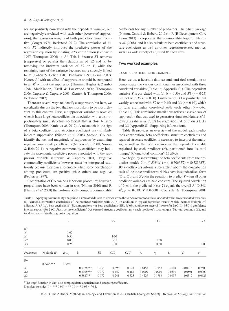
Here, we use a heuristic data set and statistical simulation to

demonstrate the various commonalities associated with three

correlated variables (Table 1a; Appendix S1). The dependent

variable Y is correlated with X1 (r = 0�50) and X3 (r = 0�25)but not with X2 (r = 0�00). Furthermore, X1 is positively, but

weakly, associated withX2 (r = 0�15) andX3 (r = 0�10), whichin turn are highly correlated with each other (r = 0�60,Table 1a). This correlationmatrix thus reflects a classic case of

suppression that was used to generate a simulated dataset (fol-

lowing Kraha et al. 2012) for regression CA of Y on X1, X2

andX3 (Appendix S1, Supporting information).

Table 1b provides an overview of the model, each predic-

tor’s contribution, beta coefficients, structure coefficients and

squared structure coefficients necessary to interpret the analy-

sis, as well as the total variance in the dependent variable

explained by each predictor (r2), partitioned into its total

‘unique’ (U) and total ‘common’ (C) effects.

We begin by interpreting the beta coefficients from the pre-

dictive model: Y = (0�508*X1) + (�0�306*X2) + (0�383*X3).Beta coefficients inform a researcher about the contribution

each of the three predictor variables have in standardized form

(ZX1, ZX2 andZX3) in the equation, to predictYwhen all other

predictor variables are held constant. The squared correlation

of Y with the predicted Y (or Y) equals the overall R2 (0�349,R2

adj. = 0�339, P < 0�0001, Courville & Thompson 2001;

Table 1. Applying commonality analysis to a simulated dataset to demonstrate the various commonalities associatedwith three correlated variables.

(a) Pearson’s correlation coefficients of the predictor variables with Y. (b) In addition to typical regression results, which includes multiple R2,

adjusted R2 (R2adj), beta coefficients1 (b), standard error or beta coefficients (SE), 95�0% confidence interval (lower) for b (CIL), 95�0% confidence

interval (upper) for b (CIU), structure coefficients1 (rs), squared structure coefficient (r2s ), each predictor’s total unique (U), total common (C), and

total variance (r2) in the regression equation

Y X1 X2 X3

(a)

Y 1�00X1 0�50 1�00X2 0�00 0�15 1�00X3 0�25 0�10 0�60 1�00

Predictors MultipleR2 R2adj b SE CIL CIU rs r2s U C r2

(b)

0�3495*** 0�3395X1 0�5076*** 0�058 0�393 0�623 0�8458 0�7153 0�2518 �0�0018 0�2500X2 �0�3058*** 0�072 �0�449 �0�163 0�0000 0�0000 0�0591 �0�0591 0�0000X3 0�3827*** 0�072 0�241 0�525 0�4229 0�1788 0�0937 �0�0312 0�06251The ‘regr’ function in yhat also computes beta coefficients and structure coefficients.

Significance codes: 0<*** 0�001<** 0�01<* 0�05<† 0�1.



Kraha et al. 2012), indicating that 34�9% of the variation in

the dependent variable is accounted for by the three indepen-

dent predictor variables. Please note that, although the predic-

tor variableX2 had zero correlation withY (Table 1a), its beta

coefficient is relatively high in the regression equation. Such a

result alerts one to the possible suppression by X2 on one or

more of the remaining variables and reinforces that beta coeffi-

cients are not direct measures of the relationships in a regres-

sion unless the predictors are perfectly uncorrelated (Courville

&Thompson 2001; Kraha et al. 2012).

Recall that the structure coefficients are the bivariate corre-

lation between Y and each of the predictors X1, X2 and X3;

thus, the squared structure coefficients (r2s ) represent the pro-

portion of variance in the regression effect explained by each

predictor alone irrespective of collinearity with other predic-

tors (Kraha et al. 2012). For instance, the r2s of X1 (0�715)shows that X1 was able to account for 71�5% of the regres-

sion effect given by the R2 (=0�349, Table 1b), which with

rounding error yields the corresponding r2 for X1

(0�715 9 0�349 = 0�250). Similarly, examining X2 (r2s = 0�00)shows that X2 shared no variance of Y, while X3 (r2s = 0�179)was able to explain 17�9% of the variation in Y.

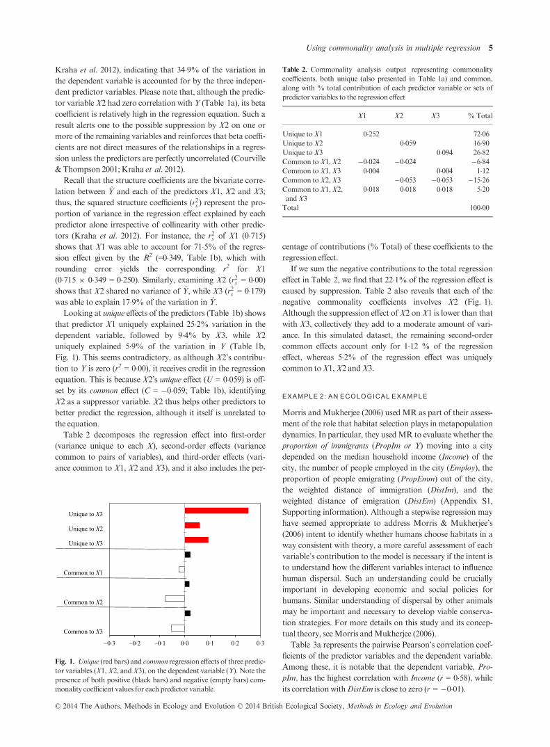
Looking at unique effects of the predictors (Table 1b) shows

that predictor X1 uniquely explained 25�2% variation in the

dependent variable, followed by 9�4% by X3, while X2

uniquely explained 5�9% of the variation in Y (Table 1b,

Fig. 1). This seems contradictory, as although X2’s contribu-

tion to Y is zero (r2 = 0�00), it receives credit in the regression

equation. This is because X2’s unique effect (U = 0�059) is off-set by its common effect (C = �0�059; Table 1b), identifying

X2 as a suppressor variable. X2 thus helps other predictors to

better predict the regression, although it itself is unrelated to

the equation.

Table 2 decomposes the regression effect into first-order

(variance unique to each X), second-order effects (variance

common to pairs of variables), and third-order effects (vari-

ance common to X1, X2 and X3), and it also includes the per-

centage of contributions (% Total) of these coefficients to the

regression effect.

If we sum the negative contributions to the total regression

effect in Table 2, we find that 22�1% of the regression effect is

caused by suppression. Table 2 also reveals that each of the

negative commonality coefficients involves X2 (Fig. 1).

Although the suppression effect ofX2 onX1 is lower than that

with X3, collectively they add to a moderate amount of vari-

ance. In this simulated dataset, the remaining second-order

common effects account only for 1�12 % of the regression

effect, whereas 5�2% of the regression effect was uniquely

common toX1,X2 andX3.

EXAMPLE 2: AN ECOLOGICAL EXAMPLE

Morris andMukherjee (2006) usedMR as part of their assess-

ment of the role that habitat selection plays in metapopulation

dynamics. In particular, they usedMR to evaluate whether the

proportion of immigrants (PropIm or Y) moving into a city

depended on the median household income (Income) of the

city, the number of people employed in the city (Employ), the

proportion of people emigrating (PropEmm) out of the city,

the weighted distance of immigration (DistIm), and the

weighted distance of emigration (DistEm) (Appendix S1,

Supporting information). Although a stepwise regression may

have seemed appropriate to address Morris & Mukherjee’s

(2006) intent to identify whether humans choose habitats in a

way consistent with theory, a more careful assessment of each

variable’s contribution to the model is necessary if the intent is

to understand how the different variables interact to influence

human dispersal. Such an understanding could be crucially

important in developing economic and social policies for

humans. Similar understanding of dispersal by other animals

may be important and necessary to develop viable conserva-

tion strategies. For more details on this study and its concep-

tual theory, seeMorris andMukherjee (2006).

Table 3a represents the pairwise Pearson’s correlation coef-

ficients of the predictor variables and the dependent variable.

Among these, it is notable that the dependent variable, Pro-

pIm, has the highest correlation with Income (r = 0�58), whileits correlationwithDistEm is close to zero (r = �0�01).

–0·3 –0·2 –0·1 0·0 0·1 0·2 0·3

Common to X3

Common to X2

Common to X1

Unique to X3

Unique to X2

Unique to X3

Fig. 1. Unique (red bars) and common regression effects of three predic-

tor variables (X1,X2, andX3), on the dependent variable (Y). Note the

presence of both positive (black bars) and negative (empty bars) com-

monality coefficient values for each predictor variable.

Table 2. Commonality analysis output representing commonality

coefficients, both unique (also presented in Table 1a) and common,

along with % total contribution of each predictor variable or sets of

predictor variables to the regression effect

X1 X2 X3 %Total

Unique toX1 0�252 72�06Unique toX2 0�059 16�90Unique toX3 0�094 26�82Common toX1,X2 �0�024 �0�024 �6�84Common toX1,X3 0�004 0�004 1�12Common toX2,X3 �0�053 �0�053 �15�26Common toX1,X2,

andX3

0�018 0�018 0�018 5�20

Total 100�00



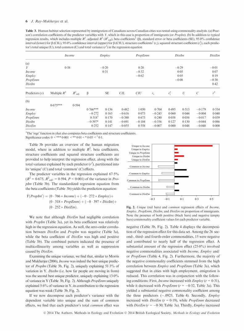
Table 3b provides an overview of the human migration

model, where in addition to multiple R2, beta coefficients,

structure coefficients and squared structure coefficients are

provided to help interpret the regression effect, along with the

total variance explained by each predictor (r2), partitioned into

its ‘unique’ (U) and total ‘common’ (C) effects.

The predictor variables in the regression explained 67�5%(R2 = 0�675, R2

adj. = 0�594, P < 0�001) of the variance in Pro-

pIm (Table 3b). The standardized regression equation from

the beta coefficients (Table 3b) yields the prediction equation:

YðPropIm0Þ ¼ ð0 � 766 � IncomeÞ þ ð�0 � 272 � EmployÞþð0 � 318 � PropEmmÞ þ ð�0 � 397 �DistImÞþð0 � 252 �DistEmÞ:

We note that although DistEm had negligible correlation

with PropIm (Table 3a), yet its beta coefficient was relatively

high in the regression equation. As well, the zero-order correla-

tion between DistEm and PropIm was negative (Table 3a),

while the beta coefficient of DistEm was high and positive

(Table 3b). The combined pattern indicated the presence of

multicollinearity among variables as well as suppression

caused byDistEm.

Examining the unique variance, we find that, similar toMorris

andMukherjee (2006), Incomewas indeed the best unique predic-

tor of PropIm (Table 3b, Fig. 2), uniquely explaining 51�3% of

variation in Y. DistIm (i.e. how far people are moving in from)

was the second best unique predictor, uniquely explaining 13�0%of variance inY (Table 3b, Fig. 2). AlthoughPropEmm uniquely

explained 5�6%of variance inY, its contribution to the regression

equationwasweak (Table 3b, Fig. 2).

If we now decompose each predictor’s variance with the

dependent variable into unique and the sum of common

effects, we find that each predictor’s total common effect was

negative (Table 3b, Fig. 2). Table 4 displays the decomposi-

tion of the regression effect for this data set. Among the 26 sec-

ond-, third- and fourth-order commonalities, 15 were negative

and contributed to nearly half of the regression effect. A

substantial amount of the regression effect (25�0%) involved

negative commonalities associated with Income, Employ and/

or PropEmm (Table 4, Fig. 2). Furthermore, the majority of

the negative commonality coefficients stemmed from the high

correlation between Employ and PropEmm (Table 3a), which

suggested that in cities with high employment, emigration is

reduced. This correlation was in conjunction with the follow-

ing conditions: First, Income increased with Employ (r = 0�31),while it decreased with PropEmm (r = �0�32, Table 3a). This

yielded a substantial negative commonality coefficient among

the three predictors (�.0925, Table 4). Secondly, Employ

increased with DistEm (r = 0�19), while PropEmm decreased

withDistEm (r = �0�30; Table 3a). Thirdly, Employ increased

Table 3. Human habitat selection represented by immigration of Canadians across Canadian cities was tested using commonality analysis. (a) Pear-

son’s correlation coefficients of the predictor variables with Y, which in this case is proportion of immigrants (or PropIm). (b) In addition to typical

regression results, which includes multiple R2, adjusted R2 (R2adj), beta coefficients1 (b), standard error or beta coefficients (SE), 95�0% confidence

interval (lower) for b (CIL), 95�0% confidence interval (upper) for b (CIU), structure coefficients1 (rs), squared structure coefficient (r2s ), each predic-

tor’s total unique (U), total common (C) and total variance (r2) in the regression equation

Income Employ PropEmm DistIm DistEm

(a)

Y 0�58 �0�20 0�20 �0�29 �0�01Income 0�31 �0�32 0�05 0�07Employ �0�62 0�05 0�19PropEmm �0�08 �0�30DistIm 0�42

Predictors (x) MultipleR2 R2adj b SE CIL CIU rs r2s U C r2

(b)

0�675*** 0�594Income 0�766*** 0�136 0�482 1�050 0�704 0�495 0�513 �0�179 0�334Employ �0�272 0�165 �0�616 0�073 �0�245 0�060 0�044 �0�004 0�040PropEmm 0�318† 0�170 �0�380 0�673 0�240 0�058 0�056 �0�017 0�039DistIm �0�397* 0�141 �0�691 �0�104 �0�356 0�127 0�130 �0�044 0�086DistEm 0�252 0�147 �0�055 0�558 �0�007 0�000 0�048 �0�048 0�0001The ‘regr’ function in yhat also computes beta coefficients and structure coefficients.

Significance codes: 0<*** 0�001<** 0�01<* 0�05<† 0�1.

–0·3 –0·1 0·1 0·3 0·5

Common to DistEm

Common to DistIm

Common to PropEmm

Common to Employ

Unique to Employ

Common to Income

Unique to DistEmUnique to DistIm

Unique to PropEmm

Unique to Income

Fig. 2. Unique (red bars) and common regression effects of Income,

Employ, PropEmm,DistIm, andDistEm on proportion of immigrants.

Note the presence of both positive (black bars) and negative (empty

bars) commonality coefficient values for each predictor variable.



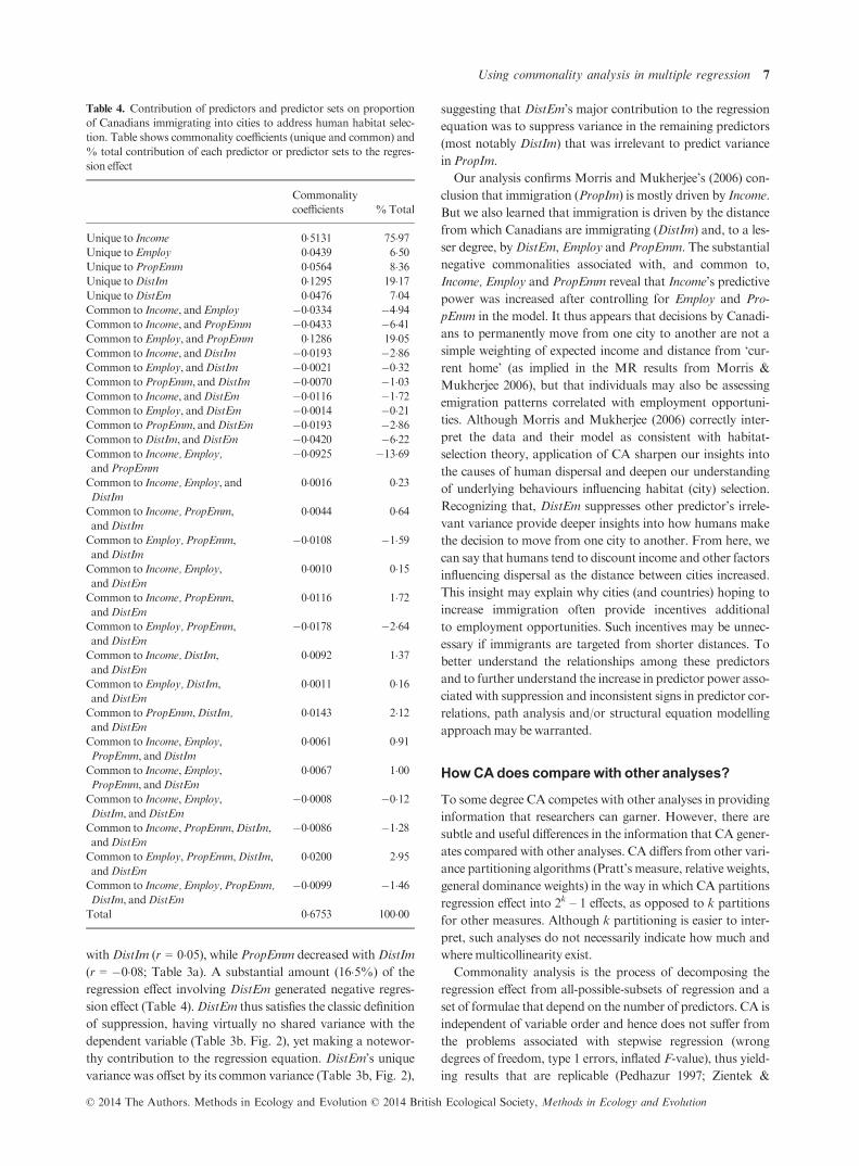
withDistIm (r = 0�05), while PropEmm decreased withDistIm

(r = �0�08; Table 3a). A substantial amount (16�5%) of the

regression effect involving DistEm generated negative regres-

sion effect (Table 4). DistEm thus satisfies the classic definition

of suppression, having virtually no shared variance with the

dependent variable (Table 3b. Fig. 2), yet making a notewor-

thy contribution to the regression equation. DistEm’s unique

variance was offset by its common variance (Table 3b, Fig. 2),

suggesting that DistEm’s major contribution to the regression

equation was to suppress variance in the remaining predictors

(most notably DistIm) that was irrelevant to predict variance

inPropIm.

Our analysis confirms Morris and Mukherjee’s (2006) con-

clusion that immigration (PropIm) is mostly driven by Income.

But we also learned that immigration is driven by the distance

from which Canadians are immigrating (DistIm) and, to a les-

ser degree, byDistEm, Employ and PropEmm. The substantial

negative commonalities associated with, and common to,

Income, Employ and PropEmm reveal that Income’s predictive

power was increased after controlling for Employ and Pro-

pEmm in the model. It thus appears that decisions by Canadi-

ans to permanently move from one city to another are not a

simple weighting of expected income and distance from ‘cur-

rent home’ (as implied in the MR results from Morris &

Mukherjee 2006), but that individuals may also be assessing

emigration patterns correlated with employment opportuni-

ties. Although Morris and Mukherjee (2006) correctly inter-

pret the data and their model as consistent with habitat-

selection theory, application of CA sharpen our insights into

the causes of human dispersal and deepen our understanding

of underlying behaviours influencing habitat (city) selection.

Recognizing that, DistEm suppresses other predictor’s irrele-

vant variance provide deeper insights into how humans make

the decision to move from one city to another. From here, we

can say that humans tend to discount income and other factors

influencing dispersal as the distance between cities increased.

This insight may explain why cities (and countries) hoping to

increase immigration often provide incentives additional

to employment opportunities. Such incentives may be unnec-

essary if immigrants are targeted from shorter distances. To

better understand the relationships among these predictors

and to further understand the increase in predictor power asso-

ciated with suppression and inconsistent signs in predictor cor-

relations, path analysis and/or structural equation modelling

approachmay be warranted.

HowCAdoes comparewith other analyses?

To some degree CA competes with other analyses in providing

information that researchers can garner. However, there are

subtle and useful differences in the information that CA gener-

ates compared with other analyses. CA differs from other vari-

ance partitioning algorithms (Pratt’s measure, relative weights,

general dominance weights) in the way in which CA partitions

regression effect into 2k – 1 effects, as opposed to k partitions

for other measures. Although k partitioning is easier to inter-

pret, such analyses do not necessarily indicate how much and

wheremulticollinearity exist.

Commonality analysis is the process of decomposing the

regression effect from all-possible-subsets of regression and a

set of formulae that depend on the number of predictors. CA is

independent of variable order and hence does not suffer from

the problems associated with stepwise regression (wrong

degrees of freedom, type 1 errors, inflated F-value), thus yield-

ing results that are replicable (Pedhazur 1997; Zientek &

Table 4. Contribution of predictors and predictor sets on proportion

of Canadians immigrating into cities to address human habitat selec-

tion. Table shows commonality coefficients (unique and common) and

% total contribution of each predictor or predictor sets to the regres-

sion effect

Commonality

coefficients %Total

Unique to Income 0�5131 75�97Unique toEmploy 0�0439 6�50Unique toPropEmm 0�0564 8�36Unique toDistIm 0�1295 19�17Unique toDistEm 0�0476 7�04Common to Income, andEmploy �0�0334 �4�94Common to Income, andPropEmm �0�0433 �6�41Common toEmploy, andPropEmm 0�1286 19�05Common to Income, andDistIm �0�0193 �2�86Common toEmploy, andDistIm �0�0021 �0�32Common toPropEmm, andDistIm �0�0070 �1�03Common to Income, andDistEm �0�0116 �1�72Common toEmploy, andDistEm �0�0014 �0�21Common toPropEmm, andDistEm �0�0193 �2�86Common toDistIm, andDistEm �0�0420 �6�22Common to Income, Employ,

andPropEmm

�0�0925 �13�69

Common to Income, Employ, and

DistIm

0�0016 0�23

Common to Income, PropEmm,

andDistIm

0�0044 0�64

Common toEmploy, PropEmm,

andDistIm

�0�0108 �1�59

Common to Income, Employ,

andDistEm

0�0010 0�15

Common to Income, PropEmm,

andDistEm

0�0116 1�72

Common toEmploy, PropEmm,

andDistEm

�0�0178 �2�64

Common to Income, DistIm,

andDistEm

0�0092 1�37

Common toEmploy, DistIm,

andDistEm

0�0011 0�16

Common toPropEmm,DistIm,

andDistEm

0�0143 2�12

Common to Income,Employ,

PropEmm, andDistIm

0�0061 0�91


PropEmm, andDistEm

0�0067 1�00


DistIm, andDistEm

�0�0008 �0�12

Common to Income,PropEmm,DistIm,

andDistEm

�0�0086 �1�28

Common toEmploy,PropEmm,DistIm,

andDistEm

0�0200 2�95

Common to Income, Employ, PropEmm,

DistIm, andDistEm

�0�0099 �1�46

Total 0�6753 100�00



Thompson 2006; Nathans, Oswald & Nimon 2012). CA may

also subsume some of the information gained through a hierar-

chical linear regression. For example, in the case of a regression

model with three predictors (X1,X2 andX3) whereX1 andX2

were entered in the first block of a hierarchical regression and

X3was added in the second block, the unique effect forX1will

be the same as the DR2 between the regression model with only

X1 and X2 and the full regression model with X1, X2 and X3.

Here, it should be kept in mind that hierarchical regressions

are different from hierarchical linearmodels.

Hierarchical linear models (also known as multilevel mod-

els, mixed models, nested models or random-effects models)

are commonly used in biological or ecological data analysis

(Nakagawa & Schielzeth 2013). CA can also be applied to

these hierarchical linear (mixed) models using the methods

described in this paper. However, instead of using R2 ana-

logues (Luo & Azen 2013; Nakagawa & Schielzeth 2013) due

to lack of monotonicity (R2 increasing with added predictors),

fit indices resulting from an all-possible-subsets analysis are

used as input to the commonality analysis algorithms

described in this paper. For a description of this solution and

the statistical software, see Nimon, Henson & Roberts (2013),

Nimon, Oswald&Roberts (2013).

Identifying the magnitude and location of multicollinearity

usingCAmay be useful in ‘fully conceptualizing and represent-

ing the regression dynamics’ (Zientek & Thompson 2006, p.

306). Structural equation models are a class of sophisticated

multivariate techniques that are largely confirmatory (based

on prior knowledge of theory) and test the validity of a model

as opposed to identifying the best model (Tomer 2003). Struc-

tural equation models explicitly address the underlying causal-

ity patterns among variables (Tomer 2003). Although CA is

applied in the same way for a given set of dependent and inde-

pendent variables regardless of one’s causal model (Pedhazur

1997), its results may be useful in identifying what causal mod-

els should be explored. In the presence of suppression, it may

be particularly useful to employ structural equation models to

assess the regression model with and without the suppressor

effects (Beckstead 2012). CA may also be used as a technique

to identify potential general factors (Hale et al. 2001); how-

ever, such analyses have been criticized and require further

research (Schneider 2008).

Limitations, conclusions and future applications

We caution readers to keep in mind that ‘methods are not a

panacea’ and require prudent use and diligent interpretation

(Kraha et al. 2012, p. 9). In regression analysis, the uniqueness

of variables depends on a specific set of predictors under study,

and the addition or deletion of predictors may change the

uniqueness attributed to some or all of the variables (Kerlinger

& Pedhazur 1973). As CA decomposes the regression effect

resulting from aMR, it is possible that failure to meet the sta-

tistical assumptions ofMRmay also impact the bias and preci-

sion of the resulting commonality coefficients; however,

research has yet to be conducted to determine how such viola-

tions of the statistical assumptions of MR affect commonality

coefficients. Understanding the complexities of ecological sys-

tems often demands collection and analysis of elaborate data

sets with confounding factors and increases in the number of

predictor variables exponentially increases the complexity of

computation and interpretation of these predictors, when con-

sidering analyses based on all possible subsets regression (e.g.

commonality analysis, dominance analysis). In such cases, it

might be advisable to conduct variance partitioning using sets

of predictors and interpret the unique and common effects of a

set of predictors (generally highly correlated family of predic-

tors), rather than single predictor variables (Zientek&Thomp-

son 2006).

Traditional MR analysis is inefficient when multicollinear

variables arise by either true synergistic association, through

spurious correlations, or by improperly specified models (Gra-

ham 2003; Whittingham et al. 2006). CA models multicollin-

ear data explicitly (Kraha et al. 2012); nevertheless, difficulties

in understanding such models should not be attributed to CA,

but to our ignorance of variables (or the model) in question.

Hence, CA should be used to identify indicators that are failing

badly with respect to the specificity of the model (Mood 1969;

Kerlinger & Pedhazur 1973). Thus, in exploratory stages of

ecological research, CA may help researchers select variables

in a predictive framework (Kerlinger & Pedhazur 1973; Pedha-

zur 1997), by revealing the confounding relationships of multi-

collinear predictor variables. Ecologists should nevertheless

use and interpret CAwith the same caution as any other analy-

sis, because it does not differentiate theoretical relationships

fromother causal relations (Kerlinger &Pedhazur 1973).

Commonality analysis has rarely been used in ecological

studies (but see Raffel et al. 2010; Sorice & Conner 2010),

and we highly recommend the use of CA when one wishes to

gain a better understanding of exploratory data. CA can

often yield additional insights into ecological studies that

have used (or plan to use) MR. Ecologists often attempt to

reduce problems of collinear variation with principal compo-

nents regression, canonical correspondence analysis, cluster

analysis and stepwise regression (Graham 2003; Araujo &

Guisan 2006; Whittingham et al. 2006). However, interpre-

tations using these techniques have not always been satisfac-

tory (Graham 2003). Regression CA can provide an

improved solution to this problem. We suggest that, along

with beta coefficients and structure coefficients (which can

also be generated using yhat package in R), CA should be

used, especially when the aim of research is exploratory.

Other approaches, such as path analysis and/or structural

equation modelling, are more appropriate when the

researcher has an prior theoretical understanding of how dif-

ferent variables and combinations of variables, are likely to

influence a particular ecological process (Morris, Dupuch &

Halliday 2012). The ability to conduct CA for a large num-

ber of variables might allow the discussion on how CA might

form the ‘missing link’ between exploratory and theory-dri-

ven research frameworks. CA thus deserves strong consider-

ation as a tool in ecological research, where it can improve

model selection and predictor contribution in regression

analysis.



Acknowledgements

We thank the Editor Prof. Bob O’Hara, the Associate Editor, Dr. Fred Oswald,

and the anonymous reviewers for helping us improve the quality of this manu-

script. JRM and SM are spouses; however, this has not influenced authorship in

themanuscript. Otherwise there is no conflict of interest among the authors.

References

Ara�ujo, M.B. & Guisan, A. (2006) Five (or so) challenges for species distribution

modeling. Journal of Biogeography, 33, 1677–1688.Beckstead, J.W. (2012) Isolating and examining sources of suppression andmulti-

collinearity in multiple linear regression.Multivariate Behavioral Research, 47,

224–246.Burnham, K.P. & Anderson, D.R. (2002)Model Selection and Multimodel Infer-

ence: A Practice Information-Theoretic Approach, 1st edn. Springer-Verlag,

NewYork.

Capraro, R.M. & Capraro, M.M. (2001) Commonality analysis: understanding

variance contributions to overall canonical correlation effects of attitude

toward mathematics on geometry achievement. Multiple Linear Regression

Viewpoints, 27, 16–23.Cohen, J. & Cohen, P. (1983) Applied Multiple Regression/Correlation Analysis

for the Behavioral Sciences, 2nd edn. Lawrence ErlbaumAssociates, Hillsdale,

New Jersey.

Conger, A.J. (1974) A revised definition for suppressor variables: a guide to their

identification and interpretation. Educational and Psychological Measurement,

34, 35–46.Courville, T. & Thompson, B. (2001) Use of structure coefficients in published

multiple regression articles: b is not enough. Educational and Psychological

Measurement, 61, 229–248.Graham, M.H. (2003) Multicollinearity in ecological multiple regression. Ecol-

ogy, 84, 2809–2815.Hale, J.B., Fiorello, C.A., Kavanagh, J.A., Hoeppner, J.B. & Gaither, R.A.

(2001)WISC-III predictors of academic achievement for childrenwith learning

disabilities: are global and factor scores comparable? School Psychology Quar-

terly, 16, 31–55.Henderson, H.V. & Velleman, P.F. (1981) Building multiple regression models

interactively.Biometrics, 37, 391–411.Kerlinger, F.N. & Pedhazur, E.J. (1973) Multiple Regression in Behavioral

Research, 1st edn.Holt, Rinehart andWinston Inc., NewYork.

Kraha, A., Turner, H., Nimon, K., Zientek, L.R. & Henson, R.K. (2012) Inter-

pretingmultiple regression in the face ofmulticollinearity. Frontiers in Psychol-

ogy, 3, 1–10.LeBreton, J.M., Ployhart, R.E. & Ladd, R.T. (2004) AMonte Carlo comparison

of relative importance methodologies. Organizational Research Methods, 7,

258–282.Lewis, M. (2007) Stepwise versus hierarchical regression: pros and cons. Paper

presented at theAnnualMeeting of the Southwest EducationalResearchAsso-

ciation, SanAntonio, TX.

Luo,W. &Azen, R. (2013) Determining predictor importance in hierarchical lin-

ear models using dominance analysis. Journal of Educational and Behavioral

Statistics, 38, 3–31.MacKinnon, D.P., Krull, J.L. & Lockwood, C.M. (2000) Equivalence of the

mediation, confounding, and suppression effect. Prevention Research, 4,

173–185.Mood, A.M. (1969) Macro-analysis of the American educational system.Opera-

tions Research, 17, 770–784.Morris, D.W., Dupuch, A. & Halliday, W.D. (2012) Climate-induced habitat

selection predicts future evolutionary strategies of lemmings. Evolutionary

EcologyResearch, 14, 689–705.Morris, D.W. & Mukherjee, S. (2006) Simulated and human metapopula-

tions created by habitat selection. Evolutionary Ecology Research, 8,

1263–1275.Nakagawa, S. & Schielzeth, H. (2013) A general and simplemethod for obtaining

R2 from generalized linear mixed-effects models.Methods in Ecology and Evo-

lution, 4, 133–142.Nathans, L., Oswald, F.L. & Nimon, K. (2012) Interpreting multiple linear

regression: a guidebook of variable importance.Practical Assessment Research

&Evaluation, 17, 1–19.Newton, R.G. & Spurrell, D. (1967) A development of multiple regression for the

analysis of routine data.Applied Statistics, 16, 51–64.Nimon, K. (2010) Regression commonality analysis: demonstration of an SPSS

solution.Multiple Linear RegressionViewpoints, 36, 10–17.Nimon, K., Henson, R. & Roberts, K. (2013) Using fit indices to holistically

assess forms of predictor importance in multilevel models. Paper presented at

the Annual Meeting of the American Psychological Association, Honolulu,

HI.

Nimon, K. & Oswald, F.L. (2013) Understanding the results of multiple linear

regression: beyond standardized regression coefficients. Organizational

ResearchMethods, 16, 650–674.Nimon, K., Oswald, F.L. & Roberts, J.K. (2013) Interpreting regression effects.

R package version 2.0-0.URL: http://cran.r-project.org/web/packages/yhat/

index.html [accessed on 17th September, 2013].

Nimon, K. & Reio, T. (2011) Regression commonality analysis: a technique

for quantitative theory building. Human Resource Development, 10, 329–340.

Nimon, K., Lewis, M., Kane, R. & Haynes, R.M. (2008) An R package to

compute commonality coefficients in multiple regression case: an introduc-

tion to the package and a practical example. Behavior Research Methods,

40, 457–466.Pedhazur, E.J. (1997) Multiple Regression in Behavioral Research: Explanation

and Prediction, 3rd edn. Harcourt Brace, Orlando, FL.

Petrocelli, J.V. (2003) Hierarchical multiple regression in counseling research:

commonproblems and possible remedies.Measurement andEvolution inCoun-

seling andDevelopment, 36, 9–22.RDevelopmentCore Team (2013)R:ALanguage and Environment for Statistical

Computing. R Foundation for Statistical Computing, Vienna. URL: http://

www.R-project.org.

Raffel, T.R., Michael, P.J., Sites, E.W. & Rohr, J.R. (2010) What drives chytrid

infections in newt populations? Associations with substrate, temperature, and

shade.EcoHealth, 7, 526–536.Schneider, W.J. (2008) Playing statistical Ouija board with commonality

analysis: good questions, wrong assumptions. Applied Neuropsychology, 15,

44–53.Siebold, D.R. & McPhee, R.D. (1979) Commonality analysis: a method for

decomposing explained variance in multiple regression analysis. Human Com-

munication Research, 5, 355–363.Smith,A.C.,Koper,N., Francis, C.M.&Fahrig, L. (2009) Confronting collinear-

ity: comparing methods for disentangling the effects of habitat loss and frag-

mentation.Landscape Ecology, 24, 1271–1285.Sokal, R.F. & Rohlf, F.J. (1995) Biometry: The Principles and Practice of Statis-

tics in Biological Research, 3rd edn.W.H. Freeman,NewYork.

Sorice, M.G. & Conner, J.R. (2010) Predicting private landowner intensions to

enroll in an incentive program to protect endangered species. Human Dimen-

sions ofWildlife, 15, 77–89.Thomas, R.D., Hughes, E. & Zumbo, B.D. (1998) On variable importance in

linear regression.Social Indicators Research, 45, 253–275.Thompson, B. (1995) Stepwise regression and stepwise discriminant analysis need

not apply here: a guidelines editorial. Educational and Psychological Measure-

ment, 55, 525–534.Thompson, B. (2006) Foundations of Behavioral Statistics: An Insight-Based

Approach, 1st edn. TheGuilford Press, NewYork.

Tomer, P. (2003) A short history of structural equation models. Structural Equa-

tion Modeling: Applications in Ecological and Evolutionary Biology (eds B.H.

Pugesek, A. Tomer & A. von Eye), pp. 85–124. Cambridge University Press,

NewYork.

Whittingham, M.J., Stephens, P.A., Bradbury, R.B. & Freckleton, R.P. (2006)

Why do we still use stepwise modeling in ecology and behaviour? Journal of

Animal Ecology, 75, 1182–1189.Zientek, L.R. & Thompson, B. (2006) Commonality analysis: partitioning vari-

ance to facilitate better understanding of data. Journal of Early Intervention, 4,

299–307.

Received 23May 2013; accepted 20 January 2014

Handling Editor: Shinichi Nakagawa

Supporting Information

Additional Supporting Information may be found in the online version

of this article.

Appendix S1.Rcodes for example 1& 2 on how to perform commonal-

ity analysis.

Appendix S2. Supportingmaterials.

Appendix S3.Human.csv



1

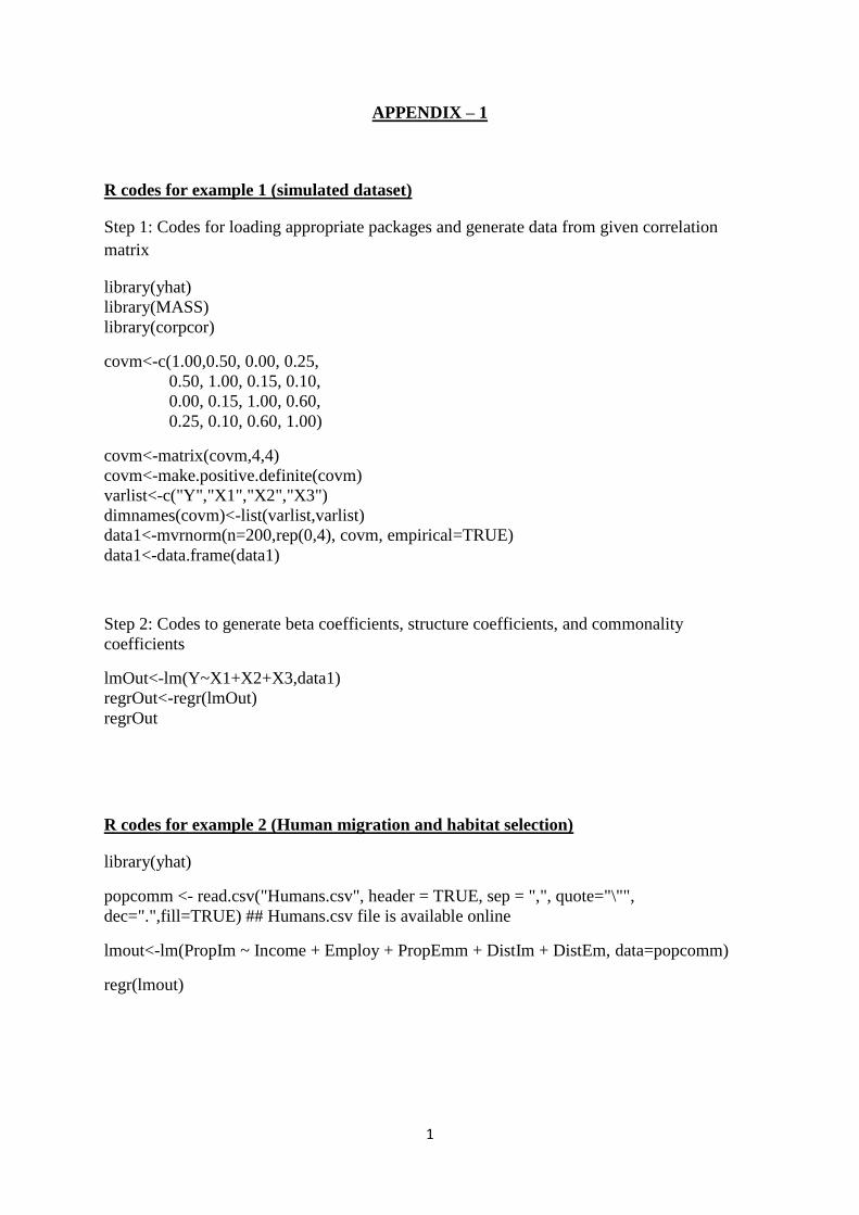
APPENDIX – 1

R codes for example 1 (simulated dataset)

Step 1: Codes for loading appropriate packages and generate data from given correlation

matrix

library(yhat)

library(MASS)

library(corpcor)

covm<-c(1.00,0.50, 0.00, 0.25,

0.50, 1.00, 0.15, 0.10,

0.00, 0.15, 1.00, 0.60,

0.25, 0.10, 0.60, 1.00)

covm<-matrix(covm,4,4)

covm<-make.positive.definite(covm)

varlist<-c("Y","X1","X2","X3")

dimnames(covm)<-list(varlist,varlist)

data1<-mvrnorm(n=200,rep(0,4), covm, empirical=TRUE)

data1<-data.frame(data1)

Step 2: Codes to generate beta coefficients, structure coefficients, and commonality

coefficients

lmOut<-lm(Y~X1+X2+X3,data1)

regrOut<-regr(lmOut)

regrOut

R codes for example 2 (Human migration and habitat selection)

library(yhat)

popcomm <- read.csv("Humans.csv", header = TRUE, sep = ",", quote="\"",

dec=".",fill=TRUE) ## Humans.csv file is available online

lmout<-lm(PropIm ~ Income + Employ + PropEmm + DistIm + DistEm, data=popcomm)

regr(lmout)

Using commonality analysis in multiple regressions:a tool to decompose regression effects in the...

Documents

Transcript of Using commonality analysis in multiple regressions:a tool to decompose regression effects in the...