INTRODUCTION

1.1 Aim of the ThesisThis project presents an interactive algorithm to

automatically segment out a person’s face from a given

image that consists of a head-and-shoulders view of the

person and a complex background scene. The method involves

a fast, reliable, and effective algorithm that exploits the

spatial distribution characteristics of human skin color.

To fulfill this aim, the following objectives are

carried out:

1. Implement different types of image segmentations.

2. A universal skin-color map is derived and used on the

chrominance component of the input image to detect

pixels with skin-color appearance .

3. Then, based on the spatial distribution of the

detected skin-color pixels and their corresponding

luminance values, the algorithm employs a set of

novel regularization processes to reinforce regions

of skin color pixels that are more likely to belong

to the facial regions and eliminate those that are

not.

4. The performance of the face segmentation algorithm is

illustrated by some simulation results carried out on

various head-and-shoulders test images.

1

1.2 Sco

pe of the Thesis

The main objective of this research is to design a

system that can find a person’s face from given image

data. This problem is commonly referred to as face

location, face extraction, or face segmentation.

Regardless of the terminology, they all share the same

objective. However, note that the problem usually deals

with finding the position and contour of a person’s face

since its location is unknown, but given the knowledge

of its existence. If this is not known, then there is

also a need to discriminate between “images containing

faces” and “images not containing faces.” This is known

as face detection. This paper, however, focuses on face

segmentation. The significance of this problem can be

illustrated by its vast applications, as face

segmentation holds an important key to future advances

in human-to-human and human-to-machine communications.

The segmentation of a facial region provides a content-

based representation of the image where it can be used

for encoding, manipulation, enhancement, indexing,

modeling, pattern-recognition, and object-tracking

purposes.

1.3 Literature Survey

2

The research on face segmentation has been pursued at

a feverish pace, there are still many problems yet to be

fully and convincingly solved as the level of difficulty of

the problem depends highly on the complexity level of the

image content and its application. Many existing methods

only work well on simple input images with a benign

background and frontal view of the person’s face. To cope

with more complicated images and conditions, many more

assumptions will then have to be made.Many of the

approaches proposed over the years involved the combination

of shape, motion, and statistical analysis. In recent

times, however, a new approach of using color information

has been introduced.

In this paper, we will discuss the color analysis

approach to face segmentation. The discussion includes the

derivation of a universal model of human skin color, the

use of appropriate color space, and the limitations of

color segmentation. We then present a practical solution to

the face-segmentation problem. This includes how to derive

a robust skin-color reference map and how to overcome the

limitations of color segmentation. In addition to face

segmentation, one of its applications on video coding will

be presented in further detail. It will explain how the

face-segmentation results can be exploited by an existing

video coder so that it encodes the area of interest (i.e.,

3

the facial region) with higher fidelity and hence produces

images with better rendered facial features.

1.4 Applications of the Thesis

Some practical applications include the following

Coding area of interest with better quality:

The subjective quality of a very low-bit-rate encoded

videophone sequence can be improved by coding the facial

image region that is of interest to viewers at higher

quality Content-based representation and MPEG-4: Face

segmentation is a useful tool for the MPEG-4 content-based

functionality. It provides content-based representation of

the image, which can subsequently be used for coding,

editing, or other interactivity purposes.

Three-dimensional (3-D) human face model fitting: The delimitation of the person’s face is the

fundamental requirement of 3-D human face model fitting

used in model-based coding, computer animation, and

morphing.

Image enhancement: Face segmentation information can be used in a post

processing task for enhancing images, such as the automatic

adjustment of tint in the facial region.

4

Face recognition: Finding the person’s face is the first important step

in the human face recognition, classification, and

identification systems.

Face tracking: Face location can be used to design a video camera

system that tracks a person’s face in a room. It can be

used as part of an intelligent vision system or simply in

video surveillance.

1.5 Organization of the Thesis

The presented project thesis is organized with 6 main

chapters. Chapter 1 gives an overview of aim of the thesis,

technical approach, Literature survey and organization of

the thesis. Chapter 2 describes the Fundamentals of image

segmentation. This chapter describes exsisting methods of

image segmentation. This chapter also gives an idea of

different file formats. Chapter 3 briefly explains about

the Color Analysis. Chapter 4 describes about the Face

segmentation Algorithm. This chapter also presents the

simulation results obtained for the implemented design.

Chapter 5 presents Conclusion and future scope with

references and appendix presented at the end.

5

6

Image segmentation

2.1 Segmentation:

In computer vision, segmentation refers to the process

of partitioning a digital image into multiple segments

(sets of pixels, also known as super pixels). The goal of

segmentation is to simplify and/or change the

representation of an image into something that is more

meaningful and easier to analyze. Image segmentation is

typically used to locate objects and boundaries (lines,

curves, etc.) in images. More precisely, image segmentation

is the process of assigning a label to every pixel in an

image such that pixels with the same label share certain

visual characteristics.

The result of image segmentation is a set of segments

that collectively cover the entire image, or a set of

contours extracted from the image (see edge detection).

Each of the pixels in a region is similar with respect to

some characteristic or computed property, such as color,

intensity, or texture. Adjacent regions are significantly

different with respect to the same characteristics.

Thresholding

Edge finding

7

Binary mathematical morphology

Gray-value mathematical morphology

In the analysis of the objects in images it

is essential that we can distinguish between the

objects of interest and "the rest." This latter group

is also referred to as the background. The techniques

that are used to find the objects of interest are

usually referred to as segmentation techniques -

segmenting the foreground from background. In this

section we will two of the most common techniques

thresholding and edge finding and we will present

techniques for improving the quality of the

segmentation result. It is important to understand

that:

1. There is no universally applicable segmentation

technique that will work for all images, and,

2. No segmentation technique is perfect.

2.1.1 THRESHOLDING:

This technique is based upon a simple concept. A

parameter called the brightness threshold is chosen and

applied to the image a [m, n] as follows:

8

This version of the algorithm assumes that we are

interested in light objects on a dark background. For dark

objects on a light background we would use:

The output is the label "object" or "background"

which, due to its dichotomous nature, can be represented as

a Boolean variable "1" or "0". In principle, the test

condition could be based upon some other property than

simple brightness (for example, If (Redness {a [m, n]} >=

θred), but the concept is clear.

The central question in thresholding then becomes: how

do we choose the threshold θ? While there is no universal

procedure for threshold selection that is guaranteed to

work on all images, there are a variety of alternatives.

Fixed threshold - One alternative is to use a threshold

that is chosen independently of the image data. If it is

known that one is dealing with very high-contrast images

where the objects are very dark and the background is

homogeneous and very light, then a constant threshold of

9

128 on a scale of 0 to 255 might be sufficiently accurate.

By accuracy we mean that the number of falsely-classified

pixels should be kept to a minimum.

Histogram-derived thresholds - In most cases the threshold

is chosen from the brightness histogram of the region or

image that we wish to segment. An image and its associated

brightness histogram are shown in Figure 2.

(a) Image to be threshold

(b) Brightness histogram of the image

Figure 2: Pixels below the threshold (a [m, n] < θ) will be

labeled as object pixels; those above the threshold will be

labeled as background pixels.

A variety of techniques have been devised to automatically

choose a threshold starting from the gray-value histogram,

{h[b] | b = 0, 1, 2B-1}. Some of the most common ones are

presented below. Many of these algorithms can benefit from

a smoothing of the raw histogram data to remove small

fluctuations but the smoothing algorithm must not shift the

peak positions. This translates into a zero-phase smoothing

10

algorithm given below where typical values for W are 3 or

5:

2.1.2 EDGE FINDING:

Thresholding produces a segmentation that yields all

the pixels that, in principle, belong to the object or

objects of interest in an image. An alternative to this is

to find those pixels that belong to the borders of the

objects. Techniques that are directed to this goal are

termed edge finding techniques. From our discussion on

mathematical morphology, specifically eqs. , and, we see

that there is an intimate relationship between edges and

regions.

Gradient-based procedure - The central challenge to

edge finding techniques is to find procedures that produce

closed contours around the objects of interest. For objects

of particularly high SNR, this can be achieved by

calculating the gradient and then using a suitable

threshold. This is illustrated in Figure 4.

11

(a) SNR = 30 dB (b) SNR = 20 dB

Figure 4: Edge finding based on the Sobel gradient, eq,

combined with the Isodata thresholding algorithm eq. . . .

While the technique works well for the 30 dB image in

Figure 4a, it fails to provide an accurate determination of

those pixels associated with the object edges for the 20 dB

image in Figure 4b. A variety of smoothing techniques as

described in Section 9.4 and in eq. can be used to reduce

the noise effects before the gradient operator is applied.

Zero-crossing based procedure - A more modern view tohandling the problem of edges in noisy images is to use the

zero crossings generated in the Laplacian of an image. The

rationale starts from the model of an ideal edge, a step

function, that has been blurred by an OTF such as Table 4

T.3 (out-of-focus), T.5 (diffraction-limited), or T.6

(general model) to produce the result shown in Figure 5.

12

Figure 5: Edge finding based on the zero crossing as

determined by the second derivative, the Laplacian. The

curves are not to scale.

The edge location is, according to the model, at that

place in the image where the Laplacian changes sign, the

zero crossing. As the Laplacian operation involves a second

derivative, this means a potential enhancement of noise in

the image at high spatial frequencies. To prevent enhanced

noise from dominating the search for zero crossings, a

smoothing is necessary.

The appropriate smoothing filter, from among the many

possibilities should according to Canny have the following

properties:

In the frequency domain, (u,v) or (Ω,ψ), the filter

should be as narrow as possible to provide suppression

of high frequency noise, and;

In the spatial domain, (x, y) or [m, n], the filter

should be as narrow as possible to provide good

localization of the edge. A too wide filter generates

uncertainty as to precisely where, within the filter

width, the edge is located.

The smoothing filter that simultaneously satisfies

both these properties--minimum bandwidth and minimum

spatial width is the Gaussian filter described. This means

13

that the image should be smoothed with a Gaussian of an

appropriate followed by application of the Laplacian. In

formula:

Where g2D(x, y). The derivative operation is linear and

shift-invariant as defined in eqs. (85) And (86). This

means that the order of the operators can be exchanged (eq.

(4)) or combined into one single filter (eq. (5)). This

second approach leads to the Marr-ildreth formulation of

the "Laplacian-of-Gaussians" (LoG) filter:

Where

Given the circular symmetry this can also be written as:

14

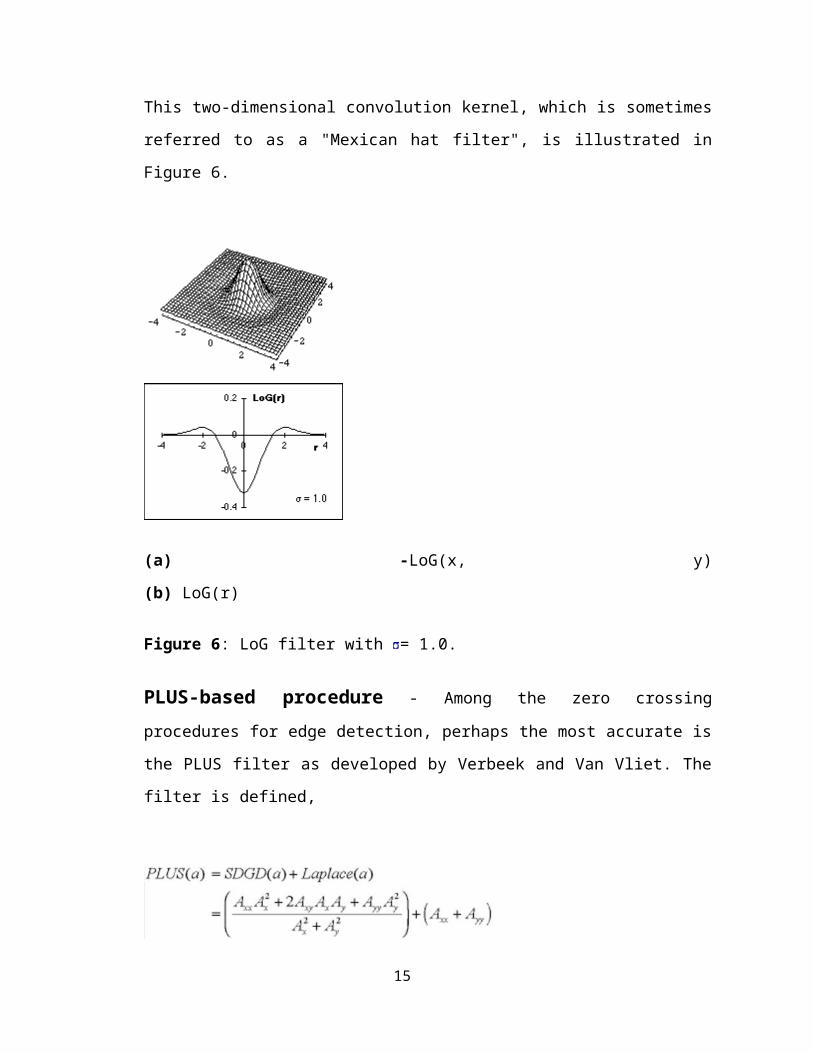
This two-dimensional convolution kernel, which is sometimes

referred to as a "Mexican hat filter", is illustrated in

Figure 6.

(a) -LoG(x, y)

(b) LoG(r)

Figure 6: LoG filter with = 1.0.

PLUS-based procedure - Among the zero crossing

procedures for edge detection, perhaps the most accurate is

the PLUS filter as developed by Verbeek and Van Vliet. The

filter is defined,

15

Neither the derivation of the PLUS's properties nor an

evaluation of its accuracy is within the scope of this

section. Suffice it to say that, for positively curved

edges in gray value images, the Laplacian-based zero

crossing procedure overestimates the position of the edge

and the SDGD-based procedure underestimates the position.

This is true in both two-dimensional and three-dimensional

images with an error on the order of (σ/R) 2 where R is the

radius of curvature of the edge.

The PLUS operator has an error on the order of (σ/R) 4 if

the image is sampled at, at least, 3x the usual Nyquist

sampling frequency or if we choose σ>= 2.7 and sample at

the usual Nyquist frequency.

All of the methods based on zero crossings in the

Laplacian must be able to distinguish between zero

crossings and zero values. While the former represent edge

positions, the latter can be generated by regions that are

no more complex than bilinear surfaces, that is, a(x,y) =

a0 + a1*x + a2*y + a3*x*y. To distinguish between these two

situations, we first find the zero crossing positions and

label them as "1" and all other pixels as "0". We then

multiply the resulting image by a measure of the edge

strength at each pixel. There are various measures for the

edge strength that are all based on the gradient as

described in Section 9.5.1 and eq. . This last possibility,

16

use of a morphological gradient as an edge strength

measure, was first described by Lee, aralick, and Shapiro

and is particularly effective. After multiplication the

image is then thresholded (as above) to produce the final

result. The procedure is thus as follows:

Figure 7: General strategy for

edges based on zero crossings.

The results of these two edge finding techniques based on

zero crossings, LoG filtering and PLUS filtering, are shown

in Figure 7 for images with a 20 dB SNR.

17

a) Image SNR = 20 dB b) LoG

filter c) PLUS filter

Figure 7: Edge finding using zero crossing algorithms LoG

and PLUS. In both algorithms σ=

Edge finding techniques provide, as the name suggests, an

image that contains a collection of edge pixels. Should the

edge pixels correspond to objects, as opposed to say simple

lines in the image, and then a region-filling technique

18

such as eq. may be required to provide the complete

objects.

2.1.3 BINARY MATHEMATICAL MORPHOLOGY

The various algorithms that we have described for

mathematical morphology in Section 9.6 can be put together

to form powerful techniques for the processing of binary

images and gray level images. As binary images frequently

result from segmentation processes on gray level images,

the morphological processing of the binary result permits

the improvement of the segmentation result.

Salt-or-pepper filtering - Segmentation procedures

frequently result in isolated "1" pixels in a "0"

neighborhood (salt) or isolated "0" pixels in a "1"

neighborhood (pepper). The appropriate neighborhood

definition must be chosen as in Figure 3. Using the lookup

table formulation for Boolean operations in a 3 x 3

neighborhood that was described in association with Figure

43, salt filtering and pepper filtering are straightforward

to implement. We weight the different positions in the 3 x

3 neighborhood as follows:

19

For a 3 x 3 window in a [m, n] with values "0" or "1" we

then compute:

The result, sum, is a number bounded by 0 <= sum <= 511.

Salt Filter The 4-connected and 8-connected versionsof this filter are the same and are given by the following

procedure:

i) Compute sum ii) If ((sum == 1) c [m, n] = 0 Else c [m,

n] = a [m, n]

Pepper Filter - The 4-connected and 8-connected versionsof this filter are the following procedures:

4-connected 8-connected i) Compute sum i) Compute sum ii)

If ( (sum == 170) ii) If ( (sum == 510) c[m,n] = 1 c[m,n] =

1 Else Else c[m,n] = a[m,n] c[m,n] = a[m,n]

Isolate objects with holes - To find objects with

holes we can use the following procedure which is

illustrated in Figure 8.

i) Segment image to produce binary mask representation

ii) Compute skeleton without end pixels

20

iii) Use salt filter to remove single skeleton pixels

iv) Propagate remaining skeleton pixels into original

binary mask.

a) Binary image b) Skeleton after salt filter c)

Objects with holes

Figure 8: Isolation of objects with holes using

morphological operations.

The binary objects are shown in gray and the

skeletons, after application of the salt filter, are shown

as a black overlay on the binary objects. Note that this

procedure uses no parameters other then the fundamental

choice of connectivity; it is free from "magic numbers." In

the example shown in Figure 58, the 8-connected definition

was used as well as the structuring element B = N8.

Filling holes in objects - To fill holes in objects weuse the following procedure which is illustrated in Figure

9.

i) Segment image to produce binary representation of

objects

21

ii) Compute complement of binary image as a mask image

iii) Generate a seed image as the border of the image

iv) Propagate the seed into the mask - eq.

v) Complement result of propagation to produce final

result

a) Mask and Seed images

b) Objects with holes filled

Figure 9: Filling holes in objects.

The mask image is illustrated in gray in Figure 9a and the

seed image is shown in black in that same illustration.

When the object pixels are specified with a connectivity of

C = 8, then the propagation into the mask (background)

image should be performed with a connectivity of C = 4,

that is, dilations with the structuring element B = N4.

This procedure is also free of "magic numbers."

22

Removing border-touching objects - Objects that areconnected to the image border are not suitable for

analysis. To eliminate them we can use a series of

morphological operations that are illustrated in Figure 10.

i) Segment image to produce binary mask image of

objects

ii) Generate a seed image as the border of the image

iii) Propagate the seed into the mask - eq.

iv) Compute XOR of the propagation result and the mask

image as final result

a) Mask and Seed images

b) Remaining objects

Figure 10: Removing objects touching borders.

23

The mask image is illustrated in gray in Figure 10a and the

seed image is shown in black in that same illustration. If

the structuring element used in the propagation is B = N4,

then objects are removed that are 4-connected with the

image boundary. If B = N8 is used then objects that 8-

connected with the boundary are removed.

Exo-skeleton - The exo-skeleton of a set of objects isthe skeleton of the background that contains the objects.

The exo-skeleton produces a partition of the image into

regions each of which contains one object. The actual

skeletonization is performed without the preservation of

end pixels and with the border set to "0." The procedure is

described below and the result is illustrated in Figure 11.

i) Segment image to produce binary image

ii) Compute complement of binary image

iii) Compute skeleton using eq. i+ii with border set to

"0"

Figure 11: Exo-skeleton.

24

2.1.4 GRAY-VALUE MATHEMATICAL MORPHOLOGY Gray-value morphological processing techniques can be

used for practical problems such as shading correction. In

this section several other techniques will be presented.

Top-hat transform - The isolation of gray-value objectsthat are convex can be accomplished with the top-hat

transform as developed by Meyer. Depending upon whether we

are dealing with light objects on a dark background or dark

objects on a light background, the transform is defined as:

Light objects -

Dark objects -

Where the structuring element B is chosen to be bigger than

the objects in question and, if possible, to have a convex

shape. Because of the properties given in eqs. And, Topat

(A, B) >= 0. An example of this technique is shown in

Figure 13.

The original image including shading is processed by a 15 x

1 structuring element as described in eqs. And to produce

the desired result. Note that the transform for dark

objects has been defined in such a way as to yield

"positive" objects as opposed to "negative" objects. Other

definitions are, of course, possible.

25

Thresholding - A simple estimate of a locally-varyingthreshold surface can be derived from morphological

processing as follows:

Threshold surface -

Once again, we suppress the notation for the structuring

element B under the max and min operations to keep the

notation simple. Its use, however, is understood.

(A) Original

(a) Light object transform (b) Dark object transform

Figure 13: Top-hat transforms.

Local contrast stretching - Using morphological

operations we can implement a technique for local contrast

stretching. That is, the amount of stretching that will be

applied in a neighborhood will be controlled by the

26

original contrast in that neighborhood. The morphological

gradient defined in eq. may also be seen as related to a

measure of the local contrast in the window defined by the

structuring element B:

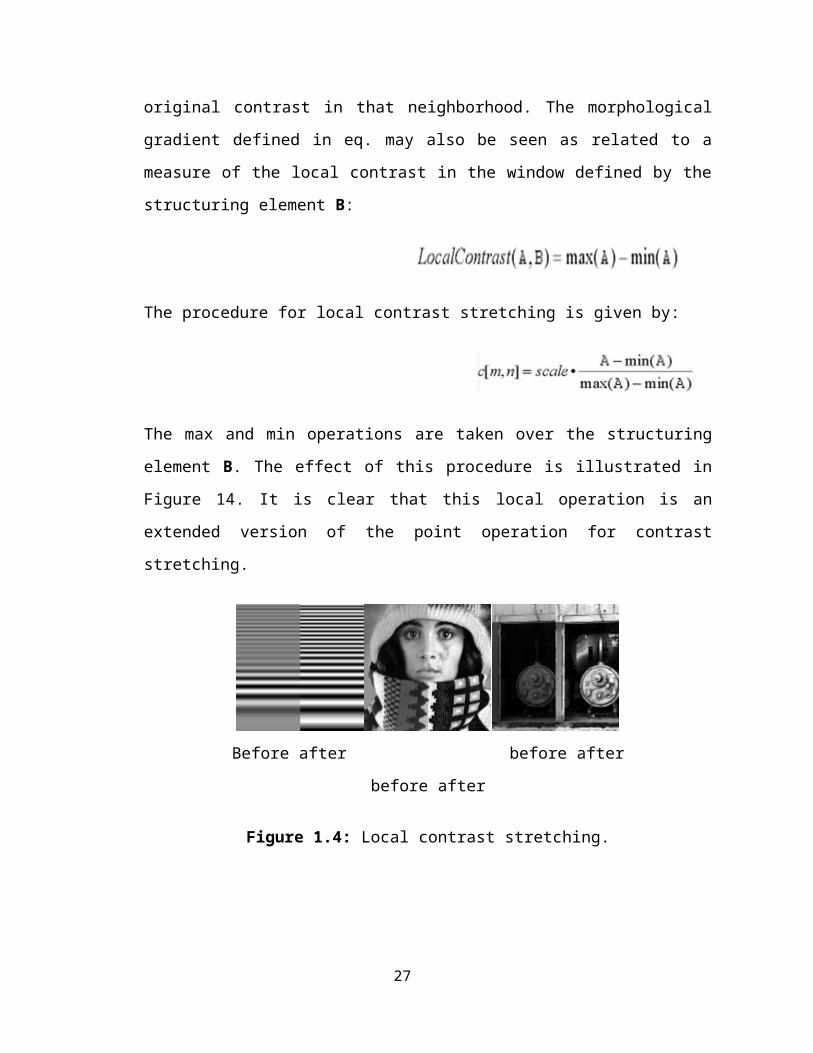
The procedure for local contrast stretching is given by:

The max and min operations are taken over the structuring

element B. The effect of this procedure is illustrated in

Figure 14. It is clear that this local operation is an

extended version of the point operation for contrast

stretching.

Before after before after

before after

Figure 1.4: Local contrast stretching.

27

Using standard test images (as we have seen in so many examples)

illustrates the power of this local morphological filtering

approach.

Facial Image Processing and Analysis:

Face recognition systems are progressively becoming

popular as means of extracting biometric information. Face

recognition has a critical role in biometric systems and is

attractive for numerous applications including visual

surveillance and security. Because of the general public

acceptance of face images on various documents, face

recognition has a great potential to become the next

generation biometric technology of choice. Face images are

also the only biometric information available in some

legacy databases and international terrorist watch-lists

and can be acquired even without subjects' cooperation.

Though there has been a great deal of progress in face

detection and recognition in the last few years, many

problems remain unsolved. Research on face detection must

confront with many challenging problems, especially when

dealing with outdoor illumination, pose variation with

large rotation angles, low image quality, low resolution,

occlusion, and background changes in complex real-life

scenes. The design of face recognition algorithms that are

effective over a wide range of viewpoints, complex outdoor28

lighting, occlusions, facial expressions, and aging of

subjects, is still a major area of research. Before one

claims that the facial image processing / analysis system

is reliable, rigorous testing and verification on real-

world datasets must be performed, including databases for

face analysis and tracking in digital video. 3D head model

assisted recognition is another research area where new

solutions are urgently needed to enhance robustness of

today's recognition systems and enable real-time, face-

oriented processing and analysis of visual data. Thus,

vigorous research is needed to solve such outstanding

challenging problems and propose advanced solutions and

systems for emerging applications of facial image

processing and analysis.

This special issue is particularly interested in recent

progress in face detection and recognition that explores

emerging themes such as digital video, 3D, near infrared,

occlusion and disguise, long-term aging, and/or the lack of

sufficient training data. Submitted articles must not have

been previously published and must not be currently

submitted for publication elsewhere. Topics of interest

include, but are not limited to, the following:

New sensors or data sources

29

 

3D-based face recognition

Near infrared imaging for face recognition

Video-based face recognition

Preprocessing

 

Image preprocessing for face detection /

recognition

Color-based facial image processing and analysis

De-blurring and super-resolution for robust face

detection / recognition

Face and feature detection

 

Face detection for best-shot selection

Facial feature detection and extraction

3D head modeling and face tracking

Methods

 

Subspace / kernel methods for face recognition

Non-linear methods for face modeling

Bionic face representation

Ensemble learning for face classification

Key problems

30

 

Outdoor illumination

Large pose variations

Mid-term and long-term aging

Occlusion and disguise

Low quality and low resolution

Generalization problem due to lack of enough

training examples

Dataset and evaluation

 

Challenging datasets

Video-based datasets

Statistical performance evaluation

Applications and other topics

  Facial gesture recognition

Real-time processing solutions and systems

Face-based surveillance, biometrics, and multimedia

applications

Face recognition in compressed domain

31

2.2Face Location:

Face Retrieval:

The face retrieval problem, known as face detection,

can be defined as follows: given an arbitrary black and

white, still image, find the location and size of every

human face it contains. There are many applications in

which human face detection plays a very important role: it

represents the first step in a fully automatic face

recognition system, it can be used in image database

32

indexing/searching by content, in surveillance systems and

in human-computer interfaces. It also provides insight on

how to approach other pattern recognition problems

involving deformable textured objects. At the same time, it

is one of the harder problems in pattern recognition.

We've designed an inductive learning detection method that

produces a maximally specific hypothesis consistent with

the training data. Three different sets of features were

considered for defining the concept of a human face. The

performance achieved is as follows: 85% detection rate, a

false alarm rate of 0.04 % of the number of windows

analyzed and 1 minute detection time on a 320 x 240 image

on a Sun Ultrasparc 1.

33

2.3Color Image Processing: Methods and Applications

Color Image Processing: Methods and

Applications embraces two decades of extraordinary growth in

the technologies and applications for color image

processing. The book offers comprehensive coverage of state-

of-the-art systems, processing techniques, and emerging

applications of digital color imaging.

To elucidate the significant progress in

specialized areas, the editors invited renowned authorities

to address specific research challenges and recent trends in

their area of expertise. The book begins by focusing on

color fundamentals, including color management, gamut

mapping, and color constancy. The remaining chapters detail

34

the latest techniques and approaches to contemporary and

traditional color image processing and analysis for a broad

spectrum of sophisticated applications, including:

Vector and semantic processing

Secure imaging

Object recognition and feature detection

Facial and retinal image analysis

Digital camera image processing

Spectral and superresolution imaging

Image and video colorization

Virtual restoration of artwork

Video shot segmentation and surveillance

2.4 Videophone Communication:

Videophone:

A videophone is a telephone with a video screen, and is

capable of full duplex (bi-directional) video and audio

transmissions for communication between people in real-time.

It was the first form of videotelephony, later to be

followed by videoconferencing, webcams, and finally

telepresence.

At the dawn of the technology, videotelephony also included

image phones which would exchange still images between units

every few seconds over conventional POTS-type telephone

35

lines, essentially the same as slow scan TV systems.

Currently videophones are particularly useful to the deaf

and speech-impaired who can use them with sign language, and

also with video relay services to communicate with hearing

persons. Videophones are also very useful to those with

mobility issues or those who are located in distant places

and are in need of telemedical or tele-educational services.

A videophone is a telephone with a video screen, and is

capable of full duplex (bi-directional) video and audio

transmissions for communication between people in real-time.

It was the first form of videotelephony, later to be

followed by videoconferencing, webcams, and finally

telepresence.

At the dawn of the technology, videotelephony also included

image phones which would exchange still images between units

every few seconds over conventional POTS-type telephone

lines, essentially the same as slow scan TV systems.

Currently videophones are particularly useful to the deaf

and speech-impaired who can use them with sign language, and

also with video relay services to communicate with hearing

persons. Videophones are also very useful to those with

mobility issues or those who are located in distant places

and are in need of telemedical or tele-educational services.

36

A videophone is a telephone with a video screen, and is

capable of full duplex (bi-directional) video and audio

transmissions for communication between people in real-time.

It was the first form of videotelephony, later to be

followed by videoconferencing, webcams, and finally

telepresence.

At the dawn of the technology, videotelephony also included

image phones which would exchange still images between units

every few seconds over conventional POTS-type telephone

lines, essentially the same as slow scan TV systems.

Currently videophones are particularly useful to the deaf

and speech-impaired who can use them with sign language, and

also with video relay services to communicate with hearing

persons. Videophones are also very useful to those with

mobility issues or those who are located in distant places

and are in need of telemedical or tele-educational services.

A videophone is a telephone with a video screen, and is

capable of full duplex (bi-directional) video and audio

transmissions for communication between people in real-time.

It was the first form of videotelephony, later to be

followed by videoconferencing, webcams, and finally

telepresence.

At the dawn of the technology, videotelephony also included

37

image phones which would exchange still images between units

every few seconds over conventional POTS-type telephone

lines, essentially the same as slow scan TV systems.

Currently videophones are particularly useful to the deaf

and speech-impaired who can use them with sign language, and

also with video relay services to communicate with hearing

persons. Videophones are also very useful to those with

mobility issues or those who are located in distant places

and are in need of telemedical or tele-educational services.

2.5 Technology:

Video coding:

Video coding is the field in electrical engineering and

computer science that deals with representation of video

data, for storage and/or transmission, for both analog and

digital video. Though video coding is often considered to be

only for natural video, it can also be applied to synthetic

(computer generated) video, i.e., graphics. Many

representations take advantage of features of the Human

Visual System to achieve an efficient representation.

The goals of video coding are to accurately represent the

video data, compactly, provide means to navigate the video

(i.e. search forwards and backwards, random access, etc) and

other additional author and content benefits such as text38

(subtitles), meta information for searching/browsing and

digital rights management.

The biggest challenge is to reduce the size of the video

data using video compression. For this reason the terms

"video coding" and "video compression" are often used

interchangeably by those who don't know the difference. The

search for efficient video compression techniques dominated

much of the research activity for video coding since the

early 1980s, the first major milestone was H.261, from which

JPEG adopted the idea of using the DCT; since then many

other advancements have been made to algorithms such as

motion estimation. Since approximately 2000 the focus has

been more on meta data and video search, resulting in MPEG-7

and MPEG-21.

H.261:

H.261 is a ITU-T video coding standard, ratified in

November 1988.[1][2] Originally designed for transmission over

ISDN lines on which data rates are multiples of 64 kbit/s.

It is one member of the H.26x family of video coding

standards in the domain of the ITU-T Video Coding Experts

Group (VCEG). The coding algorithm was designed to be able

to operate at video bit rates between 40 kbit/s and 2

Mbit/s. The standard supports two video frame sizes: CIF

(352x288 luma with 176x144 chroma) and QCIF (176x144 with39

88x72 chroma) using a 4:2:0 sampling scheme. It also has a

backward-compatible trick for sending still picture graphics

with 704x576 luma resolution and 352x288 chroma resolution

(which was added in a later revision in 1993).

2.6 History:

Whilst H.261 was preceded in 1984 by H.120 (which also

underwent a revision in 1988 of some historic importance) as

a digital video coding standard, H.261 was the first truly

practical digital video coding standard (in terms of product

support in significant quantities). In fact, all subsequent

international video coding standards (MPEG-1 Part 2,

H.262/MPEG-2 Part 2, H.263, MPEG-4 Part 2, and H.264/MPEG-4

Part 10) have been based closely on the H.261 design.

Additionally, the methods used by the H.261 development

committee to collaboratively develop the standard have

remained the basic operating process for subsequent

standardization work in the field (see S. Okubo, "Reference

model methodology-A tool for the collaborative creation of

video coding standards", Proceedings of the IEEE, vol. 83,

no. 2, Feb. 1995, pp. 139–150). The coding algorithm uses a

hybrid of motion compensated inter-picture prediction and

spatial transform coding with scalar quantization, zig-zag

scanning and entropy encoding.

40

H.261 design:

The basic processing unit of the design is called a

macroblock, and H.261 was the first standard in which the

macroblock concept appeared. Each macroblock consists of a

16x16 array of luma samples and two corresponding 8x8 arrays

of chroma samples, using 4:2:0 sampling and a YCbCr color

space.

The inter-picture prediction reduces temporal redundancy,

with motion vectors used to help the codec compensate for

motion. Whilst only integer-valued motion vectors are

supported in H.261, a blurring filter can be applied to the

prediction signal — partially mitigating the lack of

fractional-sample motion vector precision. Transform coding

using an 8x8 discrete cosine transform (DCT) reduces the

spatial redundancy. Scalar quantization is then applied to

round the transform coefficients to the appropriate

precision determined by a step size control parameter, and

the quantized transform coefficients are zig-zag scanned and

entropy coded (using a "run-level" variable-length code) to

remove statistical redundancy.

The H.261 standard actually only specifies how to decode the

video. Encoder designers were left free to design their own

encoding algorithms, as long as their output was constrained

properly to allow it to be decoded by any decoder made

41

according to the standard. Encoders are also left free to

perform any pre-processing they want to their input video,

and decoders are allowed to perform any post-processing they

want to their decoded video prior to display. One effective

post-processing technique that became a key element of the

best H.261-based systems is called deblocking filtering.

This reduces the appearance of block-shaped artifacts caused

by the block-based motion compensation and spatial transform

parts of the design. Indeed, blocking artifacts are probably

a familiar phenomenon to almost everyone who has watched

digital video. Deblocking filtering has since become an

integral part of the most recent standard, H.264 (although

even when using H.264, additional post-processing is still

allowed and can enhance visual quality if performed well).

Design refinements introduced in later standardization

efforts have resulted in significant improvements in

compression capability relative to the H.261 design. This

has resulted in H.261 becoming essentially obsolete,

although it is still used as a backward-compatibility mode

in some video conferencing systems and for some types of

internet video. However, H.261 remains a major historical

milestone in the development of the field of video coding.

2.7 Quantization:

Quantization is the procedure of constraining something from

42

a continuous set of values (such as the real numbers) to a

discrete set (such as the integers). Quantization in

specific domains is discussed in:

Quantization (signal processing)

o Quantization (image processing)

o Quantization (sound processing)

o Quantization (music)

Quantization (physics)

o Canonical quantization

o Spatial quantization

o Charge quantization

Quantization (linguistics)

Quantization (non commutative mathematics)

o Non commutative geometry

Quantization (image processing):

Quantization, involved in image processing, is a lossy

compression technique achieved by compressing a range of

values to a single quantum value. When the number of

discrete symbols in a given stream is reduced, the stream

becomes more compressible. For example, reducing the number

of colors required to represent a digital image makes it

possible to reduce its file size. Specific applications

include DCT data quantization in JPEG and DWT data

quantization in JPEG 2000.

43

Color quantization:

Color quantization reduces the number of colors used in an

image; this is important for displaying images on devices

that support a limited number of colors and for efficiently

compressing certain kinds of images. Most bitmap editors and

many operating systems have built-in support for color

quantization. Popular modern color quantization algorithms

include the nearest color algorithm (for fixed palettes),

the median cut algorithm, and an algorithm based on octrees.

It is common to combine color quantization with dithering to

create an impression of a larger number of colors and

eliminate banding artifacts.

2.8 Frequency quantization for image compression:

The human eye is fairly good at seeing small differences in

brightness over a relatively large area, but not so good at

distinguishing the exact strength of a high frequency

(rapidly varying) brightness variation. This fact allows one

to reduce the amount of information required by ignoring the

high frequency components. This is done by simply dividing

each component in the frequency domain by a constant for

that component, and then rounding to the nearest integer.

This is the main lossy operation in the whole process. As a

result of this, it is typically the case that many of the

44

higher frequency components are rounded to zero, and many of

the rest become small positive or negative numbers.

As human vision is also more sensitive to luminance than

chrominance, further compression can be obtained by working

in a non-RGB color space which separates the two (e.g.

YCbCr), and quantizing the channels separately.[1]

Quantization matrices:

A typical video codec works by breaking the picture into

discrete blocks (8×8 pixels in the case of MPEG[1]). These

blocks can then be subjected to discrete cosine transform

(DCT) to separate out the low frequency and high frequency

components in both the horizontal and vertical direction.[1]

The resulting block (the same size as the original block) is

then divided by the quantization matrix, and each entry

rounded. The coefficients of quantization matrices are often

specifically designed to keep certain frequencies in the

source to avoid losing image quality. Many video encoders

(such as DivX, Xvid, and 3ivx) and compression standards

(such as MPEG-2 and H.264/AVC) allow custom matrices to be

used. Alternatively, the extent of the reduction may be

varied by multiplying the quantizer matrix by a scaling

factor, the quantizer scale code, prior to performing the

division.[1]

45

This is an example of DCT coefficient matrix:

A common quantization matrix is:

Dividing the DCT coefficient matrix element-wise with this

quantization matrix, and rounding to integers results in:

46

For example, using −415 (the DC coefficient) and rounding to

the nearest integer

Typically this process will result in matrices with values

primarily in the upper left (low frequency) corner. By using

a zig-zag ordering to group the non-zero entries and run

length encoding, the quantized matrix can be much more

efficiently stored than the non-quantized version.

47

COLOR ANALYSIS

The use of color information has been introduced to the

face-locating problem in recent years, and it has gained

increasing attention since then. Some recent publications

that have reported this study include. They have allshown,

in one way or another, that color is a powerful descriptor

that has practical use in the extraction of face location.

The color information is typically used for region rather

than edge segmentation. We classify the region segmentation

into two general approaches, as illustrated in Fig. 1. One

approach is to employ color as a feature for partitioning an

image into a set of homogeneous regions. For instance, the

color component of the image can be used in the region

growing technique, as demonstrated in [24], or as a basis

for a simple thresholding technique, as shown in [23]. The

other approach, however, makes use of color as a feature for

identifying a specific object in an image. In this case, the

48

skin color can be used to identify the human face. This is

feasible because human faces have a special color

distribution that differs significantly (although not

entirely) from those of the background objects. Hence this

approach requires a color map that models the skin-color

distribution characteristics.

Fig. 1. The use of color information for region

segmentation.

The skin-color map can be derived in two ways on

account of the fact not all faces have identical color

features. One approach is to predefine or manually obtain

the map such that it suits only an individual color feature.

For example, here we obtain the skin-color feature of the

subject in a standard headand- shoulders test image called

Foreman. Although this is a

49

Fig. 2. Foreman image with a white contour highlighting the

facial region.

color image in YCrCb format, its gray-scale version is

shown in Fig. 2. The figure also shows a white contour

highlighting the facial region. The histograms of the color

information (i.e., Cr and Cb values) bounded within this

contour are obtained as shown in Fig. 3. The diagrams show

that the chrominance values in the facial region are

narrowly distributed, which implies that the skin color is

fairly uniform. Therefore, this individual color feature can

simply be defined by the presence of Cr values within, say,

136 and 156, and Cb values within 110 and 123. Using these

ranges of values, we managed to locate the subject’s face in

another frame of Foreman and also in a different scene (a

standard test image called Carphone), as can be seen in Fig.

4. This approach was suggested in the past by Li and50

Forchheimer in ; however, a detailed procedure on the

modeling of individual color features and their choice of

color space was not disclosed.

Fig. 3. Histograms of Cr and Cb components in the facial

region.

In another approach, the skin-color map can be designed by

adopting histograming technique on a given set of training

data and subsequently used as a reference for any human

face. Such a method was successfully adopted by the

authors,, Sobottka and Pitas, and Cornall and Pang.

Among the two approaches, the first is likely to produce

better segmentation results in terms of reliability and

accuracy by virtue of using a precise map. However, it is

realized at the expense of having a face-segmentation

process either that is too restrictive because it uses a

predefined map or requires human interaction to manually

define the necessary map. Therefore, the second approach is51

more practical and appealing, as it attempts to cater to all

personal color features in an automatic manner, albeit in a

less precise way. This, however, raises a very important

issue regarding the coverage of all human races with one

reference map. In addition, the general use of a skin-color

model for region segmentation prompts two other questions,

namely, which color space to use and how to distinguish

other parts of the body and background objects with skin-

color appearance from the actual facial region.

3.1 Color Space:An image can be presented in a number of different color

space models.

52

• RGB:

This stands for the three primary colors: red, green,

and blue. It is a hardware-oriented model and is well known

for its color-monitor display purpose.

• HSV:

An acronym for hue-saturation-value. Hue is a color

attribute that describes a pure color, while saturation defines

the relative purity or the amount of white light mixed with

a hue; value refers to the brightness of the image. This model

is commonly used for image analysis.

• YCrCb:

This is yet another hardware-oriented model.

However, unlike the RGB space, here the luminance is

separated from the chrominance data. The Y value represents

the luminance (or brightness) component, while the Cr and Cb

values, also known as the color difference signals,

represent the chrominance component of the image. These are

some, but certainly not all, of the color space models

available in image processing. Therefore, it is important to

choose the appropriate color space for modeling human skin

color. The factors that need to be considered are application

53

and effectiveness. The intended purpose of the face segmentation

will usually determine which color space to use; at the same

time, it is essential that an effective and robust skincolor

model can be derived from the given color space. For

instance, in this paper, we propose the use of the YCrCb

color space and the reason is twofold. First, an effective

use of the chrominance information for modeling human skin

color can be achieved in this color space. Second, this

format is typically used in video coding, and therefore the

use of the same, instead of another, format for segmentation

will avoid the extra computation required in conversion. On

the other hand, both Sobottka and Pitas and Saxe and Foulds

have opted for the HSV color space, as it is compatible with

human color perception, and the hue and saturation components

have been reported also to be sufficient for discriminating

color information for modeling skin color. However, this

color space is not suitable for video coding. Hunke and

Waibel and Graf et al. used a normalized RGB color space. The

normalization was employed to minimize the dependence on the

luminance values. On this note, it is interesting to point

out that unlike the YCrCb and HSV color spaces, whereby the

brightness component is decoupled from the color information

of the image, in the RGB color space it is not. Therefore,

Graf et al. have suggested preprocessing calibration in order

to cope with unknown lighting conditions. From this point of

view, the skincolor model derived from the RGB color space

54

will be inferior to those obtained from the YCrCb or HSV

color spaces. Based on the same reasoning, we hypothesize

that a skin-color model can remain effective regardless of

the variation of skin color (e.g., black, white, or yellow)

if the derivation of the model is independent of the

brightness information of the image.

3.2 Limitations of Color Segmentation

A simple region segmentation based on the skin-color

map can provide accurate and reliable results if there is a

good contrast between skin color and those of the background

objects. However, if the color characteristic of the

background is similar to that of the skin, then pinpointing

the exact face location is more difficult, as there will be

more falsely detected background regions with skin-color

appearance. Note that in the context of face segmentation,

other parts of the body are also considered as background

objects. There are a number of methods to discriminate

between the face and the background objects, including the

use of other cues such as motion and shape. Provided that

the temporal information is available and there is a priori

knowledge of a stationary background and no camera motion,

motion analysis can be incorporated into the face-

localization system to identify nonmoving skin-color regions

as background objects. Alternatively, shape analysis

55

involving ellipse fitting can also be employed to identify

the facial region from among the detected skin-color

regions. It is a common observation that the appearance of a

human face resembles an oval shape, and therefore it can be

approximated by an ellipse [2]. In this paper, however, we

propose a set of regularization processes that are based on

the spatial distribution and the corresponding luminance

values of the detected skin-color pixels. This approach

overcomes the restriction of

motion analysis and avoids the extensive computation of the

ellipse-fitting method. The details will be discussed in the

next section along with our proposed method for face

segmentation.

In addition to poor color contrast, there are other

limitations of color segmentation when an input image is

taken in some particular lighting conditions. The color

process will encounter

some difficulty when the input image has:

• a “bright spot” on the subject’s face due to reflection of

intense lighting a dark shadow on the face as a result of

the use of strong directional lighting that has partially

blackened the facial region;

• been captured with the use of color filters. Note that

these types of images (particularly in cases 1 and 2) are

56

posing great technical challenges not only to the color

segmentation approach but also to a wide range of other

facesegmentation approaches, especially those that utilize

edge image, intensity image, or facial feature-points

extraction. However, we have found that the color analysis

approach is immune to moderate illumination changes and

shading resulting from a slightly unbalanced light source,

as these conditions do not alter the chrominance

characteristics of the skin-color model.

57

FACE-SEGMENTATION ALGORITHM

In this section, we present our methodology to perform

face segmentation. Our proposed approach is automatic in the

sense that it uses an unsupervised segmentation algorithm,

and hence no manual adjustment of any design parameter is

needed in order to suit any particular input image.

Moreover, the algorithm can be implemented in real time, and

its underlying assumptions are minimal. In fact, the only

principal assumption is that the person’s face must be

present in the given image, since we are locating and not

detecting whether there is a face. Thus, the input

information required by the algorithm is a single color

image that consists of a head-andshoulders view of the

person and a background scene, and the facial region can be

as small as only a 32 32 pixels window (or 1%) of a CIF-size

(352 288) input image. The format of the input image is to

follow the YCrCb color space, based on the reason given in

the previous section. The spatial sampling frequency ratio

of Y, Cr, and Cb is 4 : 1 : 1. So, for a CIF-size image, Y

has 288 lines and 352 pixels per line, while both Cr and Cb

58

have 144 lines and 176 pixels per line each. The algorithm

consists of five operating stages, as outlined in Fig. 5. It

begins by employing a low-level process like color

segmentation in the first stage, then uses higher level

operations that involve some heuristic knowledge about the

local connectivity of the skin-color pixels in the later

stages. Thus, each stage makes full use of the result

yielded by its preceding stage in order to refine the output

result. Consequently, all the stages must be carried out

progressively according to the given sequence.

A detailed description of each stage is presented below. For

59

illustration purposes, we will use a studio-based headand-

shoulders image called Miss America to present the intermediate

results obtained from each stage of the algorithm.

A. Stage One—Color Segmentation

The first stage of the algorithm involves the use of

color information in a fast, low-level region segmentation

process. The aim is to classify pixels of the input image

into skin color and non-skin color. To do so, we have

devised a skin-color reference map in YCrCb color space.

We have found that

a skin-color

region can be

identified by

the presence of a certain set of chrominance (i.e., Cr and

Cb) values narrowly and consistently distributed in the

YCrCb color space. The location of these chrominance values

has been found and can be illustrated using the CIE

chromaticity diagram as shown in Fig. 7. We denote and as

the respective ranges of Cr and Cb values that correspond to

skin color, which subsequently define our skin-color

reference map. The ranges that we found to be the most

60

suitable for all the input images that we have tested are

and . This map has been proven, in our experiments, to be

very robust against different types of skin color. Our

conjecture is that the different skin color that we

perceived from the video image cannot be differentiated from

the chrominance information of that image region. So, a map

that is derived from Cr and Cb chrominance values will

remain effective regardless of skin-color

variation .Moreover, our intuitive justification for the

manifestation of similar Cr and Cb distributions of skin

color of all races is that the apparent difference in skin

color that viewers perceived is mainly due to the darkness

or fairness of the skin; these features are characterized by

the difference in the brightness of the color, which is

governed by Y but not Cr and Cb. With this skin-color

reference map, the color segmentation can now begin. Since

we are utilizing only the color information, the

segmentation requires only the chrominance component of the

input image. Consider an input image of pixels, for which

the dimension of Cr and Cb therefore is . The output of the

color segmentation, and hence

stage one of the algorithm, is a bitmap of size, described

as

61

The output pixel at point is classified as skin color

and set to one if both the Cr and Cb values at that point

fall inside their respective ranges and . Otherwise, the

pixel is classified as non-skin color and set to zero. To

illustrate this, we perform color segmentation on the input

image of Miss America, and the bitmap produced can be seen in

Fig. 8. The output value of one is shown in black, while the

value of zero is shown in white (this convention will be

used throughout this paper).

62

Among all the stages, this first stage is the most

vital. Based on our model of human skin color, the color

segmentation has to remove as many pixels as possible that

are unlikely to belong to the facial region while catering

for a wide variety of skin color. However, if it falsely

removes too many pixels that belong to the facial region,

then the error will propagate down the remaining stages of

the algorithm, consequently causing a failure to the entire

algorithm. Nevertheless, the result of color segmentation is

the detection of pixels in a facial area and may also

include other areas where the chrominance values coincide

with those of the skin color (as is the case in Fig. 8).

Hence the successive operating stages of the algorithm are

used to remove these unwanted areas.

B. Stage Two—Density Regularization

63

This stage considers the bitmap produced by the

previous stage to contain the facial region that is

corrupted by noise.The noise may appear as small holes on

the facial regiondue to undetected facial features such as

eyes and mouth, or it may also appear as objects with skin-

color appearance in the background scene. Therefore, this

stage performs simple morphological operations such as dilation

to fill in any small hole in the facial area and erosion to

remove any small object in the background area. The

intention is not necessarily to remove the noise entirely

but to reduce its amount and size. To distinguish between

these two areas, we first need to identify regions of the

bitmap that have higher probability of being the facial

region. The probability measure that we used is derived from

our observation that the facial color is very uniform, and

therefore the skin-color pixels belonging to the facial

region will appear in a large cluster, while the skin-color

pixels belonging to the background may appear as large

clusters or small isolated objects. Thus, we study the

density distribution of the skin-color pixels detected in

stage one. An array of density values, called density map ,

is computed as

64

It first partitions the output bitmap of stage one into

nonoverlapping groups of 4 4 pixels, then counts the number

of skin-color pixels within each group and assigns this

value to the corresponding point of the density map.

According to the density value, we classify each point into

three types, namely, zero ( ), intermediate (0 16), and full

( ). A roup of points with zero density value will

represent a nonfacial region, while a group of fulldensity

points will signify a cluster of skin-color pixels and a

high probability of belonging to a facial region. Any point

of intermediate density value will indicate the presence of

noise. The density map of Miss America with the three density

lassifications is depicted in Fig. 9. The point of zero

density is shown in white, intermediate density in gray, and

full density in black. Once the density map is derived, we

can then begin the process that we termed as density

regularization. This involves the following three steps.

1. Discard all points at the edge of the density map,i.e

set D(0,y)=d((M/8)- ,y)=D(x,0)=D(x,(N/8)-1)=0 for all

x=0,…….(M/8)-1 and y=0,……(N/8)-1

2. Erode any full_density point (i.e set to 0)if it is

surrounded by less than 5 other full_density points in

its local 3X3 neighborhood.

3. Dilate any point of either zero or intermediate-65

density (i.e set to6) if there are more than full-

density points in its local 3X3 neighborhood.

After this process,the density map is converted to the

output bitmap of stage two as

The result of stage two for the Miss America image is displayed

in Fig. 10. Note that this bitmap is now four times lower in

spatial resolution than that of the output bitmap in stage

one.

66

C. Stage Three—Luminance Regularization

We have found that in a typical videophone image, the

brightness is nonuniform throughout the facial region, while

the background region tends to have a more even distribution

of brightness. Hence, based on this characteristic,

background region that was previously detected due to its

skin-color appearance can be further eliminated. The

analysis employed in this stage involves the spatial

distribution characteristic of the luminance values since

they define the brightness of the image. We use standard

deviation as the statistical measure of the distribution.

Note that the size of the previously obtained bitmap is

67

hence each point corresponds to a group of 8 8 luminance

values, denoted by , in the original input image. For every

skin-color pixel in , we calculate the standard deviation,

denoted as , of its corresponding group of luminance values,

using

Fig. 11 depicts the standard deviation values calculated for

the Miss America image. If the standard deviation is below a

value of two, then the corresponding 8 8 pixels region is

considered too uniform and therefore unlikely to be part of

the facial region. As a result, the output bitmap of stage

three, denoted as , is derived as

The output bitmap of this stage for the Miss America image is

presented in Fig. 12. The figure shows that a significant

portion of the unwanted background region was eliminated at

this stage.

D. Stage Four—Geometric Correction

We performed a horizontal and vertical scanning process

to identify the presence of any odd structure in the

previously obtained bitmap, , and subsequently removed it.68

This is to ensure that a correct geometric shape of the

facial region is obtained. However, prior to the scanning

process, we will attempt to further remove any more noise by

using a technique similar to that initially introduced in

stage two. Therefore, a pixel in with the value of one will

remain as a detected pixel if there are more than three

other pixels, in its local 3 3 neighborhood, with the same

value. At the same time, a pixel in with a value of zero

will be reconverted to a value of one (i.e., as a potential

pixel of the facial region) if it is surrounded by more than

five pixels, in its local 3 3 neighborhood, with a value of

one. These simple procedures will ensure that noise

appearing on the facial region is filled in and that

isolated noise objects on the background are removed.

E. Stage Five—Contour Extraction

In this final stage, we convert the output bitmap of

stage four back to the dimension of . To achieve the

increase in spatial resolution, we utilize the edge

information that is already made available by the color

segmentation in stage one. Therefore, all the boundary

points in the previous bitmap will be mapped into the

corresponding group of 4 4 pixels with the value of each

pixel as defined in the output bitmap of stage one. The

representative output bitmap of this final stage of the

69

algorithm is shown in Fig. 14.

We then commence the horizontal scanning process on the

“filtered” bitmap. We search for any short continuous run of

pixels that are assigned with the value of one. For a

CIFsize image, the threshold for a group of connected pixels

to belong to the facial region is four. Therefore, any group

of less than four horizontally connected pixels with the

value of one will be eliminated and assigned to zero. A

similar process is then performed in the vertical direction.

The rationale behind this method is that, based on our

observation, any such short horizontal or vertical run of

pixels with the value of one is unlikely to be part of a70

reasonable-size and well-detected facial region. As a

result, the output bitmap of this stage should contain the

facial region with minimal or no noise.

71

Simulation Results and Discussions

The proposed skin-color reference map is intended to

work on a wide range of skin color, including that of people

of European, Asian, and African decent. Therefore, to show

that it works on subject with skin color other than white

(as is the case with the Miss America image), we have used the

same map to perform the color-segmentation process on

subjects with black and yellow skin color. The results

obtained were very good, as can be seen in Fig. 15. The

skin-color pixels were correctly identified, in both input

images, with only a small amount of noise appearing, as

expected, in the facial regions and background scenes, which

can be removed by the remaining stages of the algorithm. We

have further tested the skin-color map with 30 samples of

images. Skin colors were grouped into three classes: white,

yellow, and black. Ten samples, each of which contained the

facial region of a different subject captured in a different

lighting condition, were taken from each class to form the

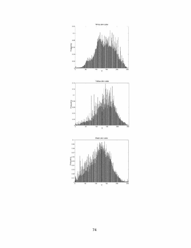
test set. We have constructed three normalized histograms

for each sample in the separate Y, Cr, and Cb components.

The rmalization process was used to account for the

variation of facial-region size in each sample. We have then

taken the average results from the ten samples of each

class. These average normalized histogram results are

presented in Fig. 16. Since all samples were taken from

different and unknown lighting conditions, the histograms of

72

the Y component for all three classes cannot be used to

verify whether the variations of luminance values in these

image samples were caused by the different skin color or by

the different lighting conditions. However, the use of such

samples illustrated that the variation in illumination does

not seem to affect the skincolor distribution in the Cr and

Cb components. On the other hand, the histograms of Cr and

Cb components for all three classes clearly showed that the

chrominance values are indeed narrowly distributed, and

more important, that the distributions are consistent across

different classes. This demonstrated that an effective skin-

color reference map could be achieved based on the Cr and Cb

components of the input image. The face-segmentation

algorithm with this universal skincolor reference map was

tested on many head-and-shoulders images. Here we emphasize

that the face-segmentation process was designed to be

completely automatic, and therefore the same design

parameters and rules (including the reference skin-color map

and the heuristic) as described in the previous section were

applied to all the test images. The test set now contained

20 images from each class of skin color. Therefore, a total

of 60 images of different subjects, background complexities,

and lighting conditions from the three classes were

73

74

75

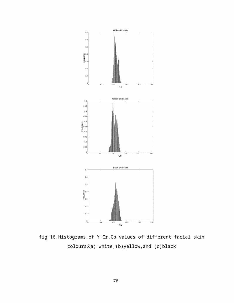
fig 16.Histograms of Y,Cr,Cb values of different facial skin

coloursa) white,(b)yellow,and (c)black

76

D. Coding Results

77

Fig. 19. (a) Foreground MB’s and (b) background MB’s (c)

coded by RM8 and (d) coded by H.261FB. (e) Magnified image

of (c). (f) Magnified image of (d).

Fig. 20. Bit rates achieved by RM8 and H.261FB coders at a

target bit rate of 192 kbits/s.

78

Fig. 21. Frame 72 of the coded results in Fig. 20: (a) RM8

and (b) H.261FB.

79

CONCLUSION

The color analysis approach to face segmentation was

discussed .In this approach the face location can be

identified by performing region segmentation with the use of

a skin color map. This is feasible because human faces have a

special color distribution characteristic that differs

significantly from those of the background objects. We have

found that pixels belonging to the facial region of the image

in YCrCb color space, exhibit similar chrominance values,

Further more a consistent range of chrominance values was

also discovered from many different facial images which

include people of European. Asian and African decent. This

led us to the derivation of a skin color map that models the

facial color of all human races . With this universal skin

color map, we classified pixels of the input image into skin

color and non skin color, Consequently, a bitmap is produced,

containing the facial region that is corrupted by noise . The

noise may appear as small holes on the facial region due to

undetected facial features or it may also appear as objects

with skin color appearance in the background scene . To cope

with this noise and at the same time refine the facial

80

region detection we have proposed a set of novel region based

regularization processes that are based on the spatial

distribution study of the detected skin color pixels and

their corresponding luminance values. All the operations are

unsupervised and low in computational complexity.

Future Scope: This project can be used to detect the skin color

of a person from the video track. In the future, this

technique can be used to detect the actual skin color of the

person. By this technique, if the skin color differs from the

actual skin color then the person will be different from the

original person.

BIBLOGRAPHY

1. D. Chai and K. N. Ngan, “Foreground/background video

coding scheme,” in Proc. IEEE Int. Symp. Circuits

Syst., Hong Kong, June 1997, vol. II, pp. 1448–1451.

2. A. Eleftheriadis and A. Jacquin, “Model-assisted

coding of video teleconferencing sequences at low bit

81

rates,” in Proc. IEEE Int. Symp. Circuits Syst.,

London, U.K., June 1994, vol. 3, pp. 177–180.

3. K. Aizawa and T. Huang, “Model-based image coding:

Advanced video coding techniques for very low-rate

applications,” Proc. IEEE, vol. 83, p. 259–271, Feb.

1995.

4. V. Govindaraju, D. B. Sher, R. K. Srihari, and S. N.

Srihari, “Locating human faces in newspaper

photographs,” in Proc. IEEE Computer Vision Pattern

Recognition Conf., San Diego, CA, June 1989, pp. 549–

554.

5. G. Sexton, “Automatic face detection for

videoconferencing,” in Proc. Inst. Elect. Eng.

Colloquium Low Bit Rate Image Coding, May 1990, pp.

9/1–9/3.

6. V. Govindaraju, S. N. Srihari, and D. B. Sher, “A

computational model for face location,” in Proc. Int.

Conf. Computer Vision, Dec. 1990, pp. 718–721.

7. H. Li, “Segmentation of the facial area for

videophone applications,” Electron. Lett., vol. 28,

pp. 1915–1916, Sept. 1992.

8. S. Shimada, “Extraction of scenes containing a

specific person from image sequences of a real-world

scene,” in Proc. IEEE TENCON’92, Melbourne, Australia,

Nov. 1992, pp. 568–572.

82

9. M. Menezes de Sequeira and F. Pereira, “Knowledge-

based videotelephone sequence segmentation,” in Proc.

SPIE Visual Commun. And Image Processing, vol. 2094,

Nov. 1993, pp. 858–869.

10. G. Yang and T. S. Huang, “Human face detection

in a complex background,” Pattern Recognit., vol. 27,

no. 1, pp. 53–63, Jan. 1994.

11. A. Eleftheriadis and A. Jacquin, “Automatic face

location detection and tracking for model-assisted

coding of video teleconferencing sequences at low-

rates,” Signal Process. Image Commun., vol. 7, nos. 4–

6, pp. 231–248, Nov. 1995.

Video track

clc;clear all;close all;[filename,pathname]=uigetfile('*.avi','select the source video');str2='.bmp';file=aviinfo(filename); %to get inforamtaion abt video filefrm_cnt=file.NumFrames ;% No.of frames in the video file frmt =aviread(filename);for i=1:25 frm(i) = aviread(filename,i);% read the Video file frm_name = frame2im(frm(i)); filename1 = strcat(num2str(i),str2); imwrite(frm_name,filename1);end%%%% face recognition in video %%%%%for p=1:25

83

filename_1=strcat((num2str(p)),str2);% form filenameI=imread(filename_1);skin_region=skin(I); %%%% from skin codingse = strel('disk',5);se2 = strel('disk',3);er = imerode(skin_region,se2);cl = imclose(er,se);dil = imdilate(cl,se); % morphologic dilationdil = imdilate(dil,se); cl2 = imclose(dil,se);d2 = imfill(cl2, 'holes');% morphologic fillfacearea = bwdist(~d2); % computing minimal euclidean distance to non-white pixel face(:,:,1)=double(I(:,:,1)).*d2; face(:,:,2)=double(I(:,:,2)).*d2; face(:,:,3)=double(I(:,:,3)).*d2; face_a=uint8(face);vwiw =strcat((num2str(p)),str2);imwrite(face_a,vwiw);endfor k=1:25 cimg=strcat(num2str(k),str2); v=imread(cimg); [Y, map] = rgb2ind(v,128); F(:,:,k)=im2frame(flipud(Y),map);end[h, w, p] = size(F(1).cdata);hf = figure('Name','TRACKED VIDEO');set(hf, 'position', [w h w h]);movie(gcf,F);delete '*.bmp'[h, w, p] = size(frm(1).cdata);hf = figure('Name','ORIGINAL VIDEO');set(hf, 'position', [w h w h]);movie(gcf,frm);

skin track

84

function segment=skin(I);I=double(I);[hue,s,v]=rgb2hsv(I);cb =0.148*I(:,:,1)-0.291*I(:,:,2)+0.439*I(:,:,3)+128;cr =0.439*I(:,:,1)-0.368*I(:,:,2)-0.071*I(:,:,3)+128;[w h]=size(I(:,:,1));for i=1:w for j=1:h if 140<=cr(i,j)&cr(i,j)<=165&140<=cb(i,j)&cb(i,j)<=195 & 0.01<=hue(i,j) & hue(i,j)<=0.1 segment(i,j)=1; else segment(i,j)=0; end endendim(:,:,1)=I(:,:,1).*segment; im(:,:,2)=I(:,:,2).*segment; im(:,:,3)=I(:,:,3).*segment;

85