Article type: Overview

Classification and Regression TreesWei-Yin Loh

University of Wisconsin, Madison, USA

Cross-References

Recursive partitioning

Keywords

Decision tree, discriminant analysis, missing value, recursive partitioning,selection bias

Abstract

Classification and regression trees are prediction models constructed by re-cursively partitioning a data set and fitting a simple model to each partition.Their name derives from the usual practice of describing the partitioning pro-cess by a decision tree. This article reviews some widely available algorithmsand compares their capabilities, strengths and weaknesses in two examples.

Classification and regression trees are machine learning methods for con-structing prediction models from data. The models are obtained by recursivelypartitioning the data space and fitting a simple prediction model within eachpartition. As a result, the partitioning can be represented graphically as a de-cision tree. Classification trees are designed for dependent variables that takea finite number of unordered values, with prediction error measured in terms ofmisclassification cost. Regression trees are for dependent variables that takecontinuous or ordered discrete values, with prediction error typically measuredby the squared difference between the observed and predicted values. Thisarticle gives an introduction to the subject by reviewing some widely availablealgorithms and comparing their capabilities, strengths and weakness in twoexamples.

Classification trees

In a classification problem, we have a training sample ofn observations on a classvariableY that takes values 1, 2, . . . ,k, andp predictor variables,X1, . . . , Xp. Ourgoal is to find a model for predicting the values ofY from newX values. In theory, thesolution is simply a partition of theX space intok disjoint sets,A1, A2, . . . , Ak, such

1

−6 −4 −2 0 2 4

−4

−2

02

46

8

X1

X2

1

1

1

1

1

11

1

11

11

1

1

1

1

11

1

12

22

2

2

2

2 2

2

2

2

2

2

2

2

2

2

2

2

2 3

3

3

3

3

3

3

33

33

3

3

3

3

33

3

3

3

X2 ≤ 0.7

X1 ≤-1.4

2 3

X1 ≤-0.6

2 1

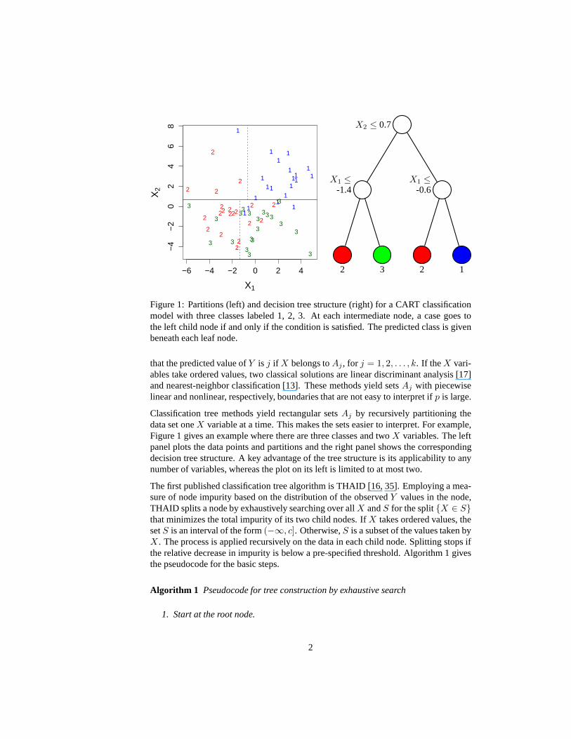
Figure 1: Partitions (left) and decision tree structure (right) for a CART classificationmodel with three classes labeled 1, 2, 3. At each intermediate node, a case goes tothe left child node if and only if the condition is satisfied. The predicted class is givenbeneath each leaf node.

that the predicted value ofY is j if X belongs toAj , for j = 1, 2, . . . , k. If theX vari-ables take ordered values, two classical solutions are linear discriminant analysis [17]and nearest-neighbor classification [13]. These methods yield setsAj with piecewiselinear and nonlinear, respectively, boundaries that are not easy to interpret ifp is large.

Classification tree methods yield rectangular setsAj by recursively partitioning thedata set oneX variable at a time. This makes the sets easier to interpret. For example,Figure 1 gives an example where there are three classes and two X variables. The leftpanel plots the data points and partitions and the right panel shows the correspondingdecision tree structure. A key advantage of the tree structure is its applicability to anynumber of variables, whereas the plot on its left is limited to at most two.

The first published classification tree algorithm is THAID [16, 35]. Employing a mea-sure of node impurity based on the distribution of the observedY values in the node,THAID splits a node by exhaustively searching over allX andS for the split{X ∈ S}that minimizes the total impurity of its two child nodes. IfX takes ordered values, thesetS is an interval of the form(−∞, c]. Otherwise,S is a subset of the values taken byX . The process is applied recursively on the data in each childnode. Splitting stops ifthe relative decrease in impurity is below a pre-specified threshold. Algorithm 1 givesthe pseudocode for the basic steps.

Algorithm 1 Pseudocode for tree construction by exhaustive search

1. Start at the root node.

2

2. For eachX , find the setS that minimizes the sum of the node impurities in thetwo child nodes and choose the split{X∗ ∈ S∗} that gives the minimum over allX andS.

3. If a stopping criterion is reached, exit. Otherwise, apply step 2 to each childnode in turn.

C4.5 [38] and CART [5] are two later classification tree algorithms that follow thisapproach. C4.5 uses entropy for its impurity function whileCART uses a generaliza-tion of the binomial variance called the Gini index. Unlike THAID, however, they firstgrow an overly large tree and then prune it to a smaller size tominimize an estimateof the misclassification error. CART employs ten-fold (default) cross-validation whileC4.5 uses a heuristic formula to estimate error rates. CART is implemented in the Rsystem [39] as RPART [43], which we use in the examples below.

Despite its simplicity and elegance, the exhaustive searchapproach has an undesirableproperty. Note that an ordered variable withm distinct values has(m − 1) splits ofthe formX ≤ c, and an unordered variable withm distinct unordered values has(2m−1 − 1) splits of the formX ∈ S. Therefore if everything else is equal, variablesthat have more distinct values have a greater chance to be selected. This selection biasaffects the integrity of inferences drawn from the tree structure.

Building on an idea that originated in the FACT [34] algorithm, CRUISE [21, 22],GUIDE [31] and QUEST [33] use a two-step approach based on significance tests tosplit each node. First, eachX is tested for association withY and the most significantvariable is selected. Then an exhaustive search is performed for the setS. BecauseeveryX has the same chance to be selected if each is independent ofY , this approach iseffectively free of selection bias. Besides, much computation is saved as the search forS is carried out only on the selectedX variable. GUIDE and CRUISE use chi-squaredtests, and QUEST uses chi-squared tests for unordered and analysis of variance testsfor ordered variables. CTree [18], another unbiased method, uses permutation tests.Pseudocode for the GUIDE algorithm is given in Algorithm 2. The CRUISE, GUIDEand QUEST trees are pruned the same way as CART.

Algorithm 2 Pseudocode for GUIDE classification tree construction

1. Start at the root node.

2. For each ordered variableX , convert it to an unordered variableX ′ by groupingits values in the node into a small number of intervals. IfX is unordered, setX ′ = X .

3. Perform a chi-squared test of independence of eachX ′ variable versusY on thedata in the node and compute its significance probability.

4. Choose the variableX∗ associated with theX ′ that has the smallest significanceprobability.

3

5. Find the split set{X∗ ∈ S∗} that minimizes the sum of Gini indexes and use itto split the node into two child nodes.

6. If a stopping criterion is reached, exit. Otherwise, apply steps 2–5 to each childnode.

7. Prune the tree with the CART method.

CHAID [20] employs yet another strategy. IfX is an ordered variable, its data valuesin the node are split into ten intervals and one child node is assigned to each interval.If X is unordered, one child node is assigned to each value ofX . Then CHAID usessignificance tests and Bonferroni corrections to try to iteratively merge pairs of childnodes. This approach has two consequences. First, some nodes may be split intomore than two child nodes. Second, owing to the sequential nature of the tests and theinexactness of the corrections, the method is biased towardselecting variables with fewdistinct values.

CART, CRUISE and QUEST can allow splits on linear combinations of all the orderedvariables while GUIDE can split on combinations of two variables at a time. If thereare missing values, CART and CRUISE use alternate splits on other variables whenneeded, C4.5 sends each observation with a missing value in asplit through everybranch using a probability weighting scheme, QUEST imputesthe missing values lo-cally, and GUIDE treats missing values as belonging to a separate category. All exceptC4.5 accept user-specified misclassification costs and all except C4.5 and CHAID ac-cept user-specified class prior probabilities. By default,all algorithms fit a constantmodel to each node, predictingY to be the class with the smallest misclassificationcost. CRUISE can optionally fit bivariate linear discriminant models and GUIDE canfit bivariate kernel density and nearest neighbor models in the nodes. GUIDE also canproduce ensemble models using bagging [3] and random forest[4] techniques. Table 1summarizes the features of the algorithms.

To see how the algorithms perform in a real application, we apply them to a data set onnew cars for the 1993 model year [26]. There are 93 cars and 25 variables. We let theYvariable be the type of drive train, which takes three values(rear, front, or four-wheeldrive). TheX variables are listed in Table 2. Three are unordered (manuf, type,andairbag, taking 31, 6, and 3 values, respectively), two binary-valued (manualanddomestic), and the rest ordered. The class frequencies are rather unequal: 16(17.2%) are rear, 67 (72.0%) are front, and 10 (10.8%) are four-wheel drive vehicles.To avoid randomness due to ten-fold cross-validation, we use leave-one-out (i.e.,n-fold) cross-validation to prune the CRUISE, GUIDE, QUEST, and RPART trees in thisarticle.

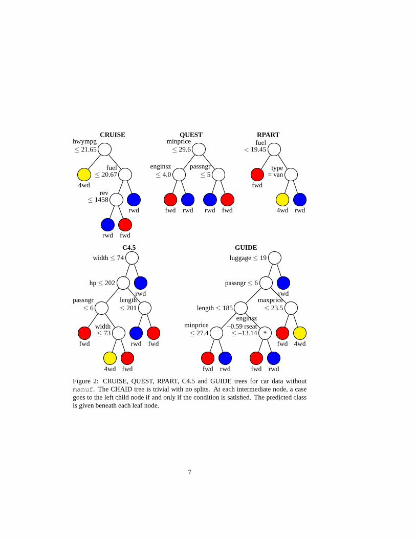
Figure 2 shows the results if the 31-valued variablemanuf is excluded. The CHAIDtree is not shown because it has no splits. The wide variety ofvariables selected in thesplits is due partly to differences between the algorithms and partly to the absence of adominantX variable. Variablepassngr is chosen by three algorithms (C4.5, GUIDEQUEST);enginsz, fuel, length, andminprice by two; andhp, hwympg,

4

Table 1 Comparison of classification tree methods. A check mark indicates pres-ence of a feature. The codes are:b = missing value branch,c = constant model,d= discriminant model,i = missing value imputation,k = kernel density model,l =linear splits,m = missing value category,n = nearest neighbor model,u = univariatesplits,s= surrogate splits,w = probability weights.

Feature C4.5 CART CHAID CRUISE GUIDE QUEST

Unbiased splits√ √ √

Split type u u,l u u,l u,l u,lBranches/split ≥2 2 ≥2 ≥2 2 2Interaction tests

√ √

Pruning√ √ √ √ √

User-specified costs√ √ √ √ √

User-specified priors√ √ √ √

Variable ranking√ √

Node models c c c c,d c,k,n cBagging & ensembles

√

Missing values w s b i,s m i

luggage, maxprice, rev, type, andwidth by one each. Variablesairbag,citympg, cylin, midprice, andrpm are not selected by any.

When GUIDE does not find a suitable variable to split a node, itlooks for a linearsplit on a pair of variables. One such split, onenginsz andrseat, occurs at thenode marked with an asterisk (*) in the GUIDE tree. Restricting the linear split to twovariables allows the data and the split to be displayed in a plot, as shown in Figure 3.Clearly, no single split on either variable alone can do as well in separating the twoclasses there.

Figure 4 shows the C4.5, CRUISE and GUIDE trees when variablemanuf is included.Now CHAID, QUEST and RPART give no splits. Comparing them with their coun-terparts in Figure 2, we see that the C4.5 tree is unchanged, the CRUISE tree has anadditional split (onmanuf), and the GUIDE tree is much shorter. This behavior isnot uncommon when there are many variables with little or no predictive power: theirintroduction can substantially reduce the size of a tree structure and its prediction ac-curacy; see, e.g., [15] for more empirical evidence.

Table 3 reports the computational times used to fit the tree models on a computer witha 2.66Ghz Intel Core 2 Quad Extreme processor. The fastest algorithm is C4.5, whichtakes milliseconds. Ifmanuf is excluded, the next fastest is RPART, at a tenth of asecond. But ifmanuf is included, RPART takes more than three hours—a105-foldincrease. This is a practical problem with the CART algorithm: becausemanuf takes31 values, the algorithm must search through230 − 1 (more than 1 billion) splits atthe root node alone. (IfY takes only two values, a computational shortcut [5, p. 101]reduces the number of searches to just 30 splits.) C4.5 is notsimilarly affected becauseit does not search for binary splits on unorderedX variables. Instead, C4.5 splits thenode into one branch for eachX value and then merges some branches after the tree

5

Table 2 Predictor variables for the car data.

Variable Description Variable Description

manuf Manufacturer (31 values) rev Engine revolutions per miletype Type (small, sporty, compact, manual Manual transmission

midsize, large, van) available (yes, no)minprice Minimum price (in $1,000) fuel Fuel tank capacity (gallons)midprice Midrange price (in $1,000) passngr Passenger capacity (persons)maxprice Maximum price (in $1,000) length Length (inches)citympg City miles per gallon whlbase Wheelbase (inches)hwympg Highway miles per gallon width Width (inches)airbag Air Bags standard (0, 1, 2) uturn U-turn space (feet)cylin Number of cylinders rseat Rear seat room (inches)enginzs Engine size (liters) luggage Luggage capacity (cu.ft.)hp Maximum horsepower weight Weight (pounds)rpm Revolutions per minute domestic Domestic (U.S./non U.S.

at maximum horsepower manufacturer)

Table 3 Tree construction times on a 2.66Ghz Intel Core 2 QuadEx-treme processor for the car data.

C4.5 CRUISE GUIDE QUEST RPART

Withoutmanuf 0.004s 3.57s 2.49s 2.26s 0.09sWith manuf 0.003s 4.00s 1.86s 2.54s 3h 2m

is grown. CRUISE, GUIDE and QUEST also are unaffected because they search ex-haustively for splits on unordered variables only if the number of values is small. If thelatter is large, these algorithms employ a technique in [34]that uses linear discriminantanalysis on dummy variables to find the splits.

6

CRUISE QUEST RPARThwympg≤ 21.65

4wd

fuel≤ 20.67

rev≤ 1458

rwd fwd

rwd

minprice≤ 29.6

enginsz≤ 4.0

fwd rwd

passngr≤ 5

rwd fwd

fuel< 19.45

fwd

type= van

4wd rwd

C4.5 GUIDE

width≤ 74

hp≤ 202

passngr≤ 6

fwd

width≤ 73

4wd fwd

length≤ 201

rwd fwd

rwd

luggage≤ 19

passngr≤ 6

length≤ 185

minprice≤ 27.4

fwd rwd

enginsz–0.59 rseat≤ –13.14 *

fwd rwd

maxprice≤ 23.5

fwd 4wd

rwd

Figure 2: CRUISE, QUEST, RPART, C4.5 and GUIDE trees for car data withoutmanuf. The CHAID tree is trivial with no splits. At each intermediate node, a casegoes to the left child node if and only if the condition is satisfied. The predicted classis given beneath each leaf node.

7

26 28 30 32 34 36

2.5

3.0

3.5

4.0

4.5

5.0

rearseat

engi

nsz

F

F

R

F

FF

F

F

R

F

F F

F

F

F

R

FR

F

R

R

F F

FF

F

R F

FR

FR

Front wheel driveRear wheel drive

Figure 3: Data and split at the node marked with an asterisk (*) in the GUIDE tree inFigure 2.

C4.5 CRUISE GUIDE

width≤ 74

hp≤ 202

passngr≤ 6

fwd

width≤ 73

4wd fwd

length≤ 201

rwd fwd

rwd

hwympg≤ 21.65

4wd

fuel≤ 20.67

rev≤ 1458

rwd

manuf

in S1

4wd

S2

rwd

S3

fwd

rwd

luggage≤ 19

fwd rwd

Figure 4: CRUISE, C4.5 and GUIDE trees for car data withmanuf included. TheCHAID, RPART and QUEST trees are trivial with no splits. SetsS1 and S2 are{Plymouth, Subaru} and{Lexus, Lincoln, Mercedes, Mercury, Volvo}, respectively,andS3 is the complement ofS1 ∪ S2.

8

Regression trees

A regression tree is similar to a classification tree, exceptthat theY variable takesordered values and a regression model is fitted to each node togive the predicted val-ues ofY . Historically, the first regression tree algorithm is AID [36], which appearedseveral years before THAID. The AID and CART regression treemethods follow Al-gorithm 1, with the node impurity being the sum of squared deviations about the meanand the node prediction the sample mean ofY . This yields piecewise constant models.Although they are simple to interpret, the prediction accuracy of these models oftenlags behind that of models with more smoothness. It can be computationally impracti-cable, however, to extend this approach to piecewise linearmodels, because two linearmodels (one for each child node) must be fitted for every candidate split.

M5’ [44], an adaptation of a regression tree algorithm due toQuinlan [37], uses amore computationally efficient strategy to construct piecewise linear models. It firstconstructs a piecewise constant tree and then fits a linear regression model to the datain each leaf node. Since the tree structure is the same as thatof a piecewise constantmodel, the resulting trees tend to be larger than those from other piecewise linear treemethods. GUIDE [27] uses classification tree techniques to solve the regression prob-lem. At each node, it fits a regression model to the data and computes the residuals.Then it defines a class variableY ′ taking values 1 or 2, depending on whether the signof the residual is positive or not. Finally it applies Algorithm 2 to theY ′ variable tosplit the node into two. This approach has three advantages:(i) the splits are unbiased,(ii) only one regression model is fitted at each node, and (iii) because it is based onresiduals, the method is neither limited to piecewise constant models nor to the leastsquares criterion. Table 4 lists the main features of CART, GUIDE and M5’.

Table 4 Comparison of regression tree methods. A check mark indicates presenceof a feature. The codes are:a = missing value category,c = constant model,g = globalmean/mode imputation,l = linear splits,m = multiple linear model,p = polynomialmodel,r = stepwise linear model,s = surrogate splits,u = univariate splits,v = leastsquares,w = least median of squares, quantile, Poisson, and proportional hazards.

Feature CART GUIDE M5’

Unbiased splits√

Split type u,l u uBranches/split 2 2 ≥2Interaction tests

√

Pruning√ √ √

Variable importance ranking√ √

Node models c c,m,p,r c,rMissing value methods s a gLoss criteria v v,w vBagging & ensembles

√

9

To compare CART, GUIDE and M5’ with ordinary least squares (OLS) linear regres-sion, we apply them to some data on smoking and pulmonary function in children [40].The data, collected from 654 children aged 3–19, give the forced expiratory volume(FEV, in liters), gender (sex, M/F), smoking status (smoke, Y/N), age (years), andheight (ht, inches) of each child. Using an OLS model for predictingFEV that in-cludes all the variables, Kahn [19] finds thatsmoke is the only one not statisticallysignificant. He also finds a significantage-smoke interaction ifht is excluded, butnot if ht and its square are both included. This problem with interpreting OLS modelsoften occurs when collinearity is present (the correlationbetween age and height is0.8).

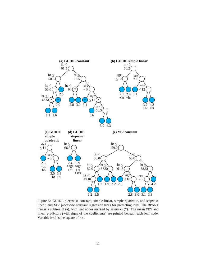
Figure 5 shows five regression tree models: (a) GUIDE piecewise constant (with sam-ple mean ofY as the predicted value in each node), (b) GUIDE best simple linear(with a linear regression model involving only one predictor in each node), (c) GUIDEbest simple quadratic regression (with a quadratic model involving only one predictorin each node), (d) GUIDE stepwise linear (with a stepwise linear regression model ineach node), and (e) M5’ piecewise constant. The CART tree (from RPART) is a sub-tree of (a), with six leaf nodes marked by asterisks (*). In the piecewise polynomialmodels (b) and (c), the predictor variable is found independently in each node, andnon-significant terms of the highest orders are dropped. Forexample for model (b) inFigure 5, a constant is fitted in the node containing females taller than 66.2, becausethe linear term forht is not significant at the 0.05 level. Similarly, two of the three leafnodes in model (c) are fitted with first degree polynomials inht because the quadraticterms are not significant. Since the nodes, and hence the domains of the polynomials,are defined by the splits in the tree, the estimated regression coefficients typically varybetween nodes.

Because the total model complexity is shared between the tree structure and the setof node models, the complexity of a tree structure often decreases as the complexityof the node models increases. Therefore the user can choose amodel by trading offtree structure complexity against node model complexity. Piecewise constant modelsare mainly used for the insights their tree structures provide. But they tend to havelow prediction accuracy, unless the data are are sufficiently informative and plentifulto yield a tree with many nodes. The trouble is that the largerthe tree, the harder it isto derive insight from it. Trees (a) and (e) are quite large, but because they split almostexclusively onht, we can infer from the predicted values in the leaf nodes thatFEVincreases monotonically withht.

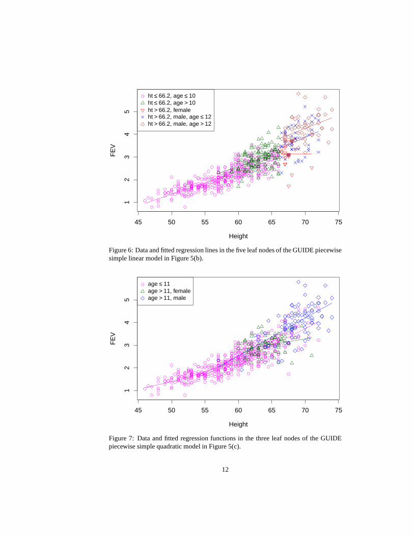
The piecewise simple linear (b) and quadratic (c) models reduce tree complexity with-out much loss (if any) of interpretability. Instead of splitting the nodes,ht now servesexclusively as the predictor variable in each node. This suggests thatht has stronglinear and possibly quadratic effects. On the other hand, the splits onage andsexpoint to interactions between them andht. These interactions can be interpreted withthe help of Figures 6 and 7, which plot the data values ofFEV andht and the fittedregression functions, with a different symbol and color foreach node. In Figure 6, theslope ofht is zero for the group of females taller than 66.2 inches, but it is constantand non-zero across the other groups. This indicates a three-way interaction involvingage, ht andsex. A similar conclusion can be drawn from Figure 7, where thereare

10

(a) GUIDE constant (b) GUIDE simple linearht≤61.5

ht≤58.5

ht≤55.0

ht ≤48.5 *

1.1 1.6

*2.0

*2.5

ht ≤66.5

ht ≤64 *

2.8 3.0

sex= F

*3.1

age≤11 *

3.6

ht ≤68.5

3.9 4.3

ht≤66.2

age≤10

2.1+ht

2.9+ht

sex= F

3.1

age≤12

3.7+ht

4.2+ht

(c) GUIDE (d) GUIDE (e) M5’ constantsimple stepwisequadratic linear

age≤11

2.3–ht

+ht2

sex= F

3.0+ht

3.9+ht

ht≤66.5

2.4+age+ht

3.9+age+ht+sex

ht ≤59.0

ht≤55.0

ht≤52.0

ht ≤49.0

1.2 1.5

1.7

ht≤57.5

1.9 2.2

ht ≤66.0

ht≤61.5

2.5

age≤10

2.8 3.0

ht≤68.5

sex= F

3.1 3.8

4.2

Figure 5: GUIDE piecewise constant, simple linear, simple quadratic, and stepwiselinear, and M5’ piecewise constant regression trees for predicting FEV. The RPARTtree is a subtree of (a), with leaf nodes marked by asterisks (*). The meanFEV andlinear predictors (with signs of the coefficients) are printed beneath each leaf node.Variableht2 is the square ofht.

11

45 50 55 60 65 70 75

12

34

5

Height

FE

V

ht ≤ 66.2, age ≤ 10ht ≤ 66.2, age > 10ht > 66.2, femaleht > 66.2, male, age ≤ 12ht > 66.2, male, age > 12

Figure 6: Data and fitted regression lines in the five leaf nodes of the GUIDE piecewisesimple linear model in Figure 5(b).

45 50 55 60 65 70 75

12

34

5

Height

FE

V

age ≤ 11age > 11, femaleage > 11, male

Figure 7: Data and fitted regression functions in the three leaf nodes of the GUIDEpiecewise simple quadratic model in Figure 5(c).

12

1 2 3 4 5

12

34

5

(a) GUIDE constant

Predicted FEV

Obs

erve

d F

EV

1 2 3 4 51

23

45

(b) GUIDE simple linear

Predicted FEV

Obs

erve

d F

EV

1 2 3 4 5

12

34

5

(c) GUIDE simple quadratic

Predicted FEV

Obs

erve

d F

EV

1 2 3 4 5

12

34

5

(d) GUIDE stepwise linear

Predicted FEV

Obs

erve

d F

EV

1 2 3 4 5

12

34

5

(e) Linear model

Predicted FEV

Obs

erve

d F

EV

1 2 3 4 5

12

34

5

(f) Linear+height^2

Predicted FEV

Obs

erve

d F

EV

Figure 8: Observed versus predicted values for the tree models in Figure 5 and twoordinary least squares models.

only three groups, with the group of children aged 11 or belowexhibiting a quadraticeffect ofht on FEV. For children above age 11, the effect ofht is linear, but maleshave, on average, about a half liter moreFEV than females. Thus the effect ofsexseems to be due mainly to children older than 11 years. This conclusion is reinforcedby the piecewise stepwise linear tree in Figure 5(d), where astepwise linear model isfitted to each of the two leaf nodes.Age andht are selected as linear predictors inboth leaf nodes, butsex is selected only in the node corresponding to children tallerthan 66.5 inches, seventy percent of whom are above 11 years old.

Figure 8 plots the observed versus predicted values of the four GUIDE models andtwo OLS models containing all the variables, without and with the square of height.The discreteness of the predicted values from the piecewiseconstant model is obvious,as is the curvature in plot (e). The piecewise simple quadratic model in plot (c) isstrikingly similar to plot (f) where the OLS model includesht-squared. This suggeststhat the two models have similar prediction accuracy. Model(c) has an advantage overmodel (f), however, because the former can be interpreted through its tree structure andthe graph of its fitted function in Figure 7.

This example shows that piecewise linear regression tree models can be valuable inproviding visual information about the roles and relative importance of the predictorvariables. For more examples, see [23, 30].

13

Conclusion

Based on published empirical comparisons of classification tree algorithms,GUIDE appears to have, on average, the highest prediction accuracy andRPART the lowest, although the differences are not substantial for univariatesplits [31]. RPART trees often have fewer leaf nodes than those of CRUISE,GUIDE and QUEST, while C4.5 trees often have the most by far. If linear com-bination splits are used, CRUISE and QUEST can yield accuracy as high as thebest non-tree methods [21, 22, 24]. The computational speed of C4.5 is almostalways the fastest while RPART can be fast or extremely slow, with the latter oc-curring when Y takes more than two values and there are unordered variablestaking many values. (Owing to its coding, the RPART software cannot acceptunordered variables with more than thirty-two values.) GUIDE piecewise linearregression tree models typically have higher prediction accuracy than piece-wise constant models. Empirical results [32] show that the accuracy of thepiecewise linear trees can be comparable to that of spline-based methods andensembles of piecewise constant trees.

Owing to space limitations, other approaches and extensions are not discussedhere. For likelihood and Bayesian approaches, see [12, 42] and [10, 14], re-spectively. For Poisson and logistic regression trees, see [8, 29] and [6, 28],respectively. For quantile regression trees, see [9]. For regression trees ap-plicable to censored data, see [1, 2, 11, 25, 41]. Asymptotic theory for theconsistency of the regression tree function and derivative estimates may befound in [7, 8, 23]. The C source code for C4.5 may be obtained fromhttp://www.rulequest.com/Personal/. RPART may be obtained fromhttp://www.R-project.org. M5’ is part of the WEKA [44] package athttp://www.cs.waikato.ac.nz/ml/weka/. Software for CRUISE, GUIDEand QUEST may be obtained from http://www/stat.wisc.edu/∼loh/.

References

[1] H. Ahn. Tree-structured exponential regression modeling. Biometrical Journal,36:43–61, 2007.

[2] H. Ahn and W.-Y. Loh. Tree-structured proportional hazards regression model-ing. Biometrics, 50:471-485, 1994.

[3] L. Breiman. Bagging predictors. Machine Learning, 24:123–140, 1996.

[4] L. Breiman. Random forests. Machine Learning, 45:5–32, 2001.

[5] L. Breiman, J. H. Friedman, R. A. Olshen, and C. J. Stone. Classification andRegression Trees. CRC Press, 1984.

[6] K.-Y. Chan and W.-Y. Loh. LOTUS: An algorithm for building accurate and com-prehensible logistic regression trees. Journal of Computational and GraphicalStatistics, 13:826–852, 2004.

14

[7] P. Chaudhuri, M.-C. Huang, W.-Y. Loh, and R. Yao. Piecewise-polynomial re-gression trees. Statistica Sinica, 4:143-167, 1994.

[8] P. Chaudhuri, W.-D. Lo, W.-Y. Loh, and C.C. Yang. Generalized regressiontrees. Statistica Sinica, 5:641-666, 1995.

[9] P. Chaudhuri and W.-Y. Loh. Nonparametric estimation of conditional quantilesusing quantile regression trees. Bernoulli, 8:561–576, 2002.

[10] H. A. Chipman, E. I. George, and R. E. McCulloch. Bayesian CART modelsearch (with discussion). Journal of the American Statistical Association, 93:935–960, 1998.

[11] H. J. Cho and S. M. Hong. Median regression tree for analysis of censoredsurvival data. IEEE Transactions on Systems, Man, and Cybernetics, Part A,383:715–726, 2008.

[12] A. Ciampi. Generalized regression trees. Computational Statistics and DataAnalysis, 12:57–78, 1991.

[13] T. Cover and P. Hart. Nearest neighbor pattern classification. IEEE Transac-tions on Information Theory, 13(1):21–27, 1967.

[14] D. G. T. Denison, B. K. Mallick, and A. F. M. Smith. A Bayesian CART algo-rithm. Biometrika, 85(2):362–377, 1998.

[15] K. Doksum, S. Tang, and K.-W. Tsui. Nonparametric variable selection: TheEARTH algorithm. Journal of the American Statistical Association, 103(484):1609–1620, 2008.

[16] A. Fielding and C. A. O’Muircheartaigh. Binary segmentation in survey analy-sis with particular reference to AID. The Statistician, 25:17–28, 1977.

[17] R. A. Fisher. The use of multiple measurements in taxonomic problems. Annalsof Eugenics, 7:179–188, 1936.

[18] T. Hothorn, K. Hornik, and A. Zeileis. Unbiased recursive partitioning: A condi-tional inference framework. Journal of Computational and Graphical Statistics,15(3):651–674, 2006.

[19] M. Kahn. An exhalent problem for teaching statis-tics. Journal of Statistics Education, 13(2), 2005.www.amstat.org/publications/jse/v13n2/datasets.kahn.html.

[20] G. V. Kass. An exploratory technique for investigating large quantities of cate-gorical data. Applied Statistics, 29:119-127, 1980.

[21] H. Kim and W.-Y. Loh. Classification trees with unbiased multiway splits. Jour-nal of the American Statistical Association, 96:589–604, 2001.

15

[22] H. Kim and W.-Y. Loh. Classification trees with bivariate linear discriminantnode models. Journal of Computational and Graphical Statistics, 12:512–530,2003.

[23] H. Kim, W.-Y. Loh, Y.-S. Shih, and P. Chaudhuri. Visualizable and interpretableregression models with good prediction power. IIE Transactions, 39:565-579,2007.

[24] T.-S. Lim, W.-Y. Loh, and Y.-S. Shih. A comparison of prediction accuracy, com-plexity, and training time of thirty-three old and new classification algorithms.Machine Learning, 40:203–228, 2000.

[25] M. LeBlanc and J. Crowley. Relative risk trees for censored survival data. Bio-metrics, 48(2):411–424, 1992.

[26] R. H. Lock. 1993 New car data. Journal of Statistics Education, 1(1), 1993.www.amstat.org/publications/jse/v1n1/datasets.lock.html

[27] W.-Y. Loh. Regression trees with unbiased variable selection and interactiondetection. Statistica Sinica, 12:361–386, 2002.

[28] W.-Y. Loh. Logistic regression tree analysis. In Handbook of Engineering Statis-tics, H. Pham (ed.), Springer, 537–549, 2006.

[29] W.-Y. Loh. Regression tree models for designed experiments. Second E.L. Lehmann Symposium, Institute of Mathematical Statistics Lecture Notes-Monograph Series, 49:210-228, 2006.

[30] W.-Y. Loh. Regression by parts: Fitting visually interpretable models withGUIDE. In Handbook of Data Visualization, C. Chen, W. Hardle, and A. Unwin(eds.), Springer, 447-469, 2008.

[31] W.-Y. Loh. Improving the precision of classification trees. Annals of AppliedStatistics, 3:1710–1737, 2009.

[32] W.-Y. Loh, C.-W. Chen and W. Zheng. Extrapolation errors in linear modeltrees. ACM Transactions on Knowledge Discovery from Data, 1(2), 2007.

[33] W.-Y. Loh and Y.-S. Shih. Split selection methods for classification trees. Sta-tistica Sinica, 7:815–840, 1997.

[34] W.-Y. Loh and N. Vanichsetakul. Tree-structured classification via generalizeddiscriminant analysis (with discussion). Journal of the American Statistical As-sociation, 83:715–728, 1988.

[35] R. Messenger and L. Mandell. A modal search technique for predictive nominalscale multivariate analysis. Journal of the American Statistical Association, 67:768–772, 1972.

[36] J. N. Morgan and J. A. Sonquist. Problems in the analysis of survey data, anda proposal. Journal of the American Statistical Association, 58:415–434, 1963.

16

[37] J. R. Quinlan. Learning with continuous classes. Proceedings of the 5th Aus-tralian Joint Conference on Artificial Intelligence, 343–348, 1992.

[38] J. R. Quinlan. C4.5: Programs for Machine Learning. Morgan Kaufmann, SanMateo, 1993.

[39] R Development Core Team. R: A Language and Environment for StatisticalComputing. R Foundation for Statistical Computing, Vienna, Austria, 2009.

[40] B. Rosner. Fundamentals of Biostatistics, 5th edition. Duxbury, Pacific Grove,1999.

[41] M. R. Segal. Regression trees for censored data. Biometrics, 44:35–47, 1988.

[42] X. Su, M. Wang, and J. Fan. Maximum likelihood regression trees. Journal ofComputational and Graphical Statistics, 13:586–598, 2004.

[43] T. M. Therneau and B. Atkinson. RPART: Recursive partitioning. R port by B.Ripley. R package version 3.1-41, 2008.

[44] I. Witten and E. Frank. Data Mining: Practical Machine Learning Tools andTechniques, 2nd edition. Morgan Kaufmann, San Francisco, 2005.

Further Reading

E. Alpaydin. Introduction to Machine Learning, 2nd edition, MIT Press, 2010.

Notes

CART R© is a registered trademark of California Statistical Software, Inc.

17