This is a preprint version of the paper accepted for publication in Language Learning.

Calculating the relative importance of multiple regression predictor variables using dominance

analysis and random forests

Atsushi Mizumoto (Kansai University, Osaka, Japan)

Abstract:

Researchers often make claims regarding the importance of predictor variables in multiple regression

analysis by comparing standardized regression coefficients (standardized beta coefficients). This

practice has been criticized as a misuse of multiple regression analysis. As a remedy, I highlight the

use of dominance analysis and random forest, a machine learning technique, in this method showcase

article to accurately determine predictor importance in multiple regression analysis. To demonstrate

the utility of dominance analysis and random forest, I reproduced the results of an empirical study

and applied these analytical procedures. The results reconfirmed that multiple regression analysis

should always be accompanied by dominance analysis and random forest to identify the unique

contribution of individual predictors while considering correlations among predictors. A web

application to facilitate the use of dominance analysis and random forest among second language

researchers is also introduced.

Keywords: multiple regression analysis; predictor importance; relative importance; dominance

analysis; random forest

Author Note:

I would like to thank Dr. Kristopher Kyle and Dr. Scott Crossley, Associate Editors of Language

Learning, and the four anonymous reviewers for their very helpful suggestions in improving the

quality of this paper. Writing this paper was supported by JSPS KAKENHI Grant Numbers

21H00553 and 20H01284. On a personal note, I would like to dedicate this paper to Dr. Hiroaki

“Keiroh” Maeda, who pointed out the misuse of standardized beta in interpreting the causal

relationship between predictor variables and the criterion variable in the early 2000s (Maeda, 2004).

Regrettably, he passed away on October 10, 2014, at the age of 40. Because I would not be who I am

today without his guidance, let me write this message to him here. “Keiroh-sensei, I’m sorry it took

so long to deliver your message. I hope you like it.”

1

1. The Problem

Multiple regression analysis has been used extensively in second language (L2) studies as an

intermediate-level statistical technique (Khany & Tazik, 2019). This correlation-based technique is

used to examine the relationship between multiple predictor variables (PVs, or the independent

variables) and a single criterion variable (CV, or the dependent variable) (Jeon, 2015). Its primary

purpose is to develop the best model, often with a linear equation, to predict the CV using a set of

PVs. In the process of generating the best fitting model with the highest explanatory power (i.e., the

amount of variance in the CV explained by the set of PVs: R2), it is also possible to assess the

relative importance or contribution of each PV to the overall effect (R2) by comparing the

standardized beta (β) coefficients. L2 researchers often make theoretical and pedagogical claims

based on the magnitude of the standardized beta coefficients, although their use as an index of

predictor importance is now considered a misuse of multiple regression analysis (Karpen, 2017).

This paper addresses this pervasive problem in L2 studies and highlights the use of dominance

analysis, one method of relative importance analysis, along with random forests as alternatives to

standardized beta coefficients to facilitate better interpretation of predictor importance.

The crux of this problem in L2 studies can be portrayed in the following example. Table 1

presents the correlation and standardized beta coefficients from a mock study (adapted from Maeda,

2004). In this hypothetical study (N = 100), we are interested in investigating the contribution of

specific skills to students’ speaking ability. Thus, the CV is “Speaking,” and the PVs are

2

“Vocabulary,” “Grammar,” “Writing,” and “Reading.” The overall variance explained (R2) is .47

(95% CI [.31, .57]). This means that 47% of the variance of the CV can be predicted from the PVs

(the predictive power of the model is 47%), and the remaining variance, or 53%, is unexplained by

the model.

We first examine the simple correlation coefficients, which are also called zero-order or

bivariate correlations, between the CV (i.e., Speaking) and each of the PVs. We can evaluate the

strength of the effect of each PV on the CV using simple correlation/regression because it is a one-

to-one comparison (see the left gray column in Table 1). It is also the starting point of any analysis.

However, this method does not consider the correlations among PVs that are likely present in reality.

Therefore, multiple regression is more appropriate and necessary to fully describe the relationship

between the CV and PVs while accounting for the shared variance among the PVs (Plonsky &

Oswald, 2017).

Table 1

Correlations and Standardized Beta Coefficients in a Mock Study (Adapted from Maeda, 2004)

Variables R

β p Speaking Vocabulary Grammar Writing Reading

Speaking ― ― ―

Vocabulary .62 ― .47 < .001

Grammar .43 .67 ― -.19 .10

Writing .56 .55 .67 ― .31 .02

Reading .61 .72 .65 .79 ― .15 .30 Note. N = 100, R2 = .47 (95% CI [.31, .57])

3

The standardized beta coefficients (β) obtained from a multiple regression analysis (see the

right gray column in Table 1) describe the direct relationship between the CV and each PV while

controlling for the indirect effects of the other PVs. As the standardized beta coefficient of a PV

represents the mean change of the CV given a one-unit (i.e., standard deviation) shift in the PV, it is

often used to compare the relative strength of the CVs in the regression model. In the example above,

Vocabulary has the largest standardized beta coefficient (β = .47). Thus, a standard deviation

increase of one in Vocabulary leads to a standard deviation expected score change of 0.47 in

Speaking (the PV) while the effects of the other PVs are controlled (i.e., all intercorrelations between

PVs are zero).

However, we notice that the magnitude of the standardized beta coefficients of Reading (β

= .15) and Grammar (β = -.19) differs in comparison to their correlation coefficients (r = .61 and .43,

respectively). This phenomenon is counterintuitive, but it is known as a suppression (or suppressor)

effect and often occurs in multiple regression analysis (Hair et al., 2019). A suppression effect arises

when one of the PVs (i.e., Grammar) is more strongly correlated with the other PVs (e.g.,

Vocabulary) than with the CV (Speaking).

Mathematically, the suppression effect is relatively easy to explain. In a situation where the CV

(Y) is explained by the two PVs (X1 and X2), the equation below shows how the standardized beta

coefficient for X1 can be derived from the correlations among them. The denominator of the equation

4

being the same (as there are only two predictors in this specific example), assuming that both the

correlation between Y and X2 and that between X1 and X2 are positive and larger than the correlation

between Y and X1, the standardized beta coefficient (β1) will be negative despite an initial positive

association in a simple correlation with Y.

!! = $"#! − $"#"$#!#"

1 −$#!#"$

The same situation happens with the regression result in Table 1 and the negative standardized

beta coefficient for Grammar (β = -.19), suggesting that Grammar has a negative effect on Speaking

and can be considered a statistical artifact. Put another way, when considering the effect of Grammar

on Speaking, much of the variance shared by these variables can be accounted for by the other PVs

that highly or moderately correlate with Grammar and Speaking. If the indirect effects of these PVs

are removed, what is left (i.e., correlations of the residuals) does not accurately show the variable

importance of Grammar. Without realizing such a statistical artifact, unwary researchers may ignore

PVs that have lower or negative standardized beta coefficients; this may result in a belief that

weighed PVs that remain in the regression model are more important than the other PVs.

Figure 1 further illustrates the relationship between the simple correlation coefficients and the

standardized beta coefficients in a path model (Oswald, 2021). As described in Figure 1, the

suppression effect persists and cannot be solved using standardized parameter estimates in structural

5

equation modeling (SEM), an advanced statistical technique that is well suited to modeling and

handling measurement errors. The same applies to SEM with latent variables (Maassen & Bakker,

2001).

Figure 1

The Relationship Between Correlations and Standardized Beta Coefficients in a Path Model

(Oswald, 2021). CC BY-SA 4.0.

6

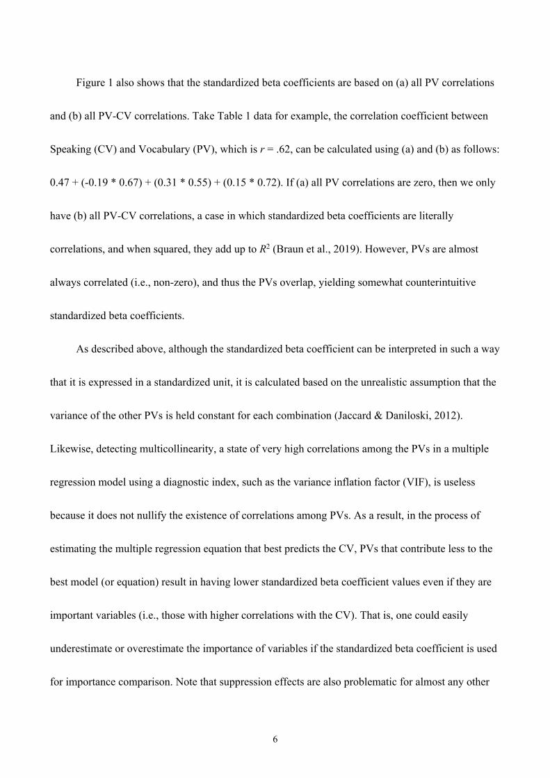
Figure 1 also shows that the standardized beta coefficients are based on (a) all PV correlations

and (b) all PV-CV correlations. Take Table 1 data for example, the correlation coefficient between

Speaking (CV) and Vocabulary (PV), which is r = .62, can be calculated using (a) and (b) as follows:

0.47 + (-0.19 * 0.67) + (0.31 * 0.55) + (0.15 * 0.72). If (a) all PV correlations are zero, then we only

have (b) all PV-CV correlations, a case in which standardized beta coefficients are literally

correlations, and when squared, they add up to R2 (Braun et al., 2019). However, PVs are almost

always correlated (i.e., non-zero), and thus the PVs overlap, yielding somewhat counterintuitive

standardized beta coefficients.

As described above, although the standardized beta coefficient can be interpreted in such a way

that it is expressed in a standardized unit, it is calculated based on the unrealistic assumption that the

variance of the other PVs is held constant for each combination (Jaccard & Daniloski, 2012).

Likewise, detecting multicollinearity, a state of very high correlations among the PVs in a multiple

regression model using a diagnostic index, such as the variance inflation factor (VIF), is useless

because it does not nullify the existence of correlations among PVs. As a result, in the process of

estimating the multiple regression equation that best predicts the CV, PVs that contribute less to the

best model (or equation) result in having lower standardized beta coefficient values even if they are

important variables (i.e., those with higher correlations with the CV). That is, one could easily

underestimate or overestimate the importance of variables if the standardized beta coefficient is used

for importance comparison. Note that suppression effects are also problematic for almost any other

7

form of relative importance indices. Partial or semi-partial correlations and changes in R2 also suffer

from the same limitation because they treat PVs as uncorrelated; as such, these indices do not

accurately reflect predictor importance (Karpen, 2017).

In the same line of discussion, standardized beta coefficients obtained from regularized

(penalized) regression, which uses alternative fitting procedures such as ridge regression (Hoerl &

Kennard, 1970), also do not make up an adequate predictor importance index. Regularized regression

is known to be effective for dealing with (a) correlated PVs and (b) a case where the number of

variables exceeds that of observations (cases) in the sample (Hair et al., 2019). In such a situation,

overfitting may occur. Overfitting (or overtraining) is a phenomenon where a model fits the training

data on which a model is built too well and fails to replicate the same performance on the test or

unseen data. In contrast to the ordinary least squares (OLS) estimates, on which a normal regression

model is based and which tend to suffer overfitting, regularized regression (also known as shrinkage

or constrained) methods shrink the estimated coefficients (e.g., standardized beta) toward zero, based

on a tuning parameter λ (lambda), relative to the OLS estimates. As a result, regularized regression

can yield better prediction accuracy and model interpretability than can the OLS estimates (James et

al., 2013). However, standardized beta coefficients obtained by applying regularized regression do

not dramatically differ from those calculated using the OLS estimates. In fact, standardized beta

coefficients applying ridge regression to the data presented in Table 1 are regularized, but they are

still similar to those using the OLS estimates (regularized betas for Vocabulary = .37; Grammar =

8

-.10; Writing = .24; Reading = .19, see online supplimentary material for the result of ridge

regression). It can thus be concluded that using regularized regression such as ridge regression may

increase prediction accuracy, but interpreting the regularized standardized beta coefficients regarding

predictor importance is still not a solution but a problem.

The examples in this section clearly indicate that one cannot rely on standardized beta

coefficients to determine predictor importance. Unfortunately, the misuse of standardized beta

coefficients in multiple regression analysis to determine important predictors has continued to this

day in the L2 research community. Therefore, the purpose of this showcase article is to call for

greater attention to L2 researchers’ misuse of multiple regression analysis and to draw readers’

attention to simple alternatives, dominance analysis and random forest, each of which has been

suggested and shown to be effective in other fields. By using such alternatives, L2 researchers are

expected to be able to better interpret variable importance in multiple regression analysis.

In the following sections, first, the solution is described. I demonstrate the effectiveness of

applying the solution to real-world problems by presenting an empirical example. Next, I introduce

an R-based web application that will enable readers to trace the results and explore the analysis in a

hands-on manner.

R version 4.0.3 (R Core Team, 2021) was used in the analyses. To ensure reproducibility and

transparency in the data analysis (Larson-Hall & Plonsky, 2015), all data and R code used in this

study are available in the IRIS repository (https://www.iris-

9

database.org/iris/app/home/detail?id=york:940279) and the Open Science Framework

(https://osf.io/uxdwh/). Furthermore, the R code can be accessed on Google Colaboratory

(https://bit.ly/3kV45pf), an online cloud-based environment that requires no setup to use. Readers

can run and examine the code and obtain the same results without even installing R and related

packages on their computer.

2. Methods for Determining Predictor Importance

2.1. Relative Importance Metrics

As demonstrated in the previous section, the standardized beta coefficient is not a proper

measure of predictor importance. In the past decade in other research fields, researchers who

recognized this problem have increasingly turned to relative importance analysis as a supplement for

regression analysis (Tonidandel & LeBreton, 2011). Relative importance analysis, also known as

“key driver analysis” in marketing research (Garver & Williams, 2020), is an umbrella term for any

technique to uncover the contributions of correlated predictors in a regression model and estimate

their importance. Relative importance analysis “produces superior estimates of correlated predictors’

importance in both simulation studies and primary studies” (Karpen, 2017, p. 84).

Several researchers have compared a range of relative importance metrics. In addition to

standardized beta coefficients (beta weight) and zero-order correlation coefficients, Table 2

summarizes relative importance measures reported in a guidebook of variable importance (Nathans

et al., 2012). As these metrics represent different perspectives on the data structure in a regression

10

model, no single relative importance metric is sufficient to fully describe the relative importance of

variables. For this reason, researchers need to select and report an appropriate variable importance

metric that suits the purpose of their research.

2.2. Dominance Analysis

Among the relative importance metrics in Table 2, dominance analysis (Budescu, 1993) and

relative weight analysis (Johnson, 2000) are the most commonly used and reported as the

recommended procedures for identifying the relative importance of PVs (Stadler et al., 2017). In the

field of L2 research, Larson-Hall (2016) introduced a method to compute the relative importance

metric (i.e., dominance analysis) using the relaimpo package of R (Grömping, 2006). However,

relative importance analysis has yet to be utilized in L2 research except for a few recent reports (e.g.,

Kyle et al., 2021), primarily because researchers are unaware of it as a viable alternative to

appropriately estimate predictor importance. As discussed earlier, correlations among PVs cause the

problem of inflating or deflating the standardized beta coefficients. That is, in an unrealistic situation

in which PVs are not correlated at all, standardized beta coefficients are a precise measure of

predictor importance. However, for real-world data, dominance analysis or relative weight analysis

could be utilized to effectively address correlations among PVs.

11

Table 2

Metrics of Relative Importance, Their Purpose, and Other Characteristics

Metric Purpose Effect Other Characteristics Zero-order correlation

Identifies magnitude and direction of the relationship between the PV and CV without considering any other PVs Direct See Figure 1

Standardized beta Identifies contribution of each PV to the CV with holding all other PVs constant Total Equivalent to correlation

if PVs uncorrelated Product measure (Pratt measure)

Partitions the regression effect into nonoverlapping partitions based on multiplying the beta of each PV with its respective correlation with the PV

Direct Total Always total R2

Structure coefficient

Identifies how much variance in the predicted scores of the CV can be attributed to each PV Direct Can identify a suppressor

Commonality analysis

Identifies how much variance in the PV is uniquely explained by each possible PV set; yields unique and common effects that, respectively, identify variance unique to one PV and multiple PVs

Total Always total R2; Can identify suppressor or multicollinearity

Dominance analysis

Indicates whether one PV contributes more variance than another PV, either (a) across all possible submodels (i.e., complete dominance) or (b) on average across models of all-possible-subset sizes (i.e., conditional dominance); averaging conditional dominance weights yields general dominance weights

Direct Total Partial

Always total R2; Can identify suppressor

Relative weight Identifies variable importance based on method that addresses multicollinearity by creating variables’ uncorrelated “counterparts” Total Always total R2

Note. Adapted from Hair et al. (2019), Nathans et al. (2012), and Nimon and Oswald (2013). PV = predictor variable (independent variable); CV = criterion variable (dependent variable); Direct (effect) = variable importance when measured in isolation from other PVs; Total (effect) = variable importance when contributions of all other PVs have been accounted for; Partial (effect) = variable importance when contribution to regression models of a specific subset or subsets of other PVs have been accounted for. All-possible-subsets regression is not included because it is not strictly a measure of relative importance; instead, it serves as a base for commonality and dominance analysis (Nimon & Oswald, 2013).

12

Dominance analysis (DA), also known as Shapley value regression, estimates the relative

importance of predictors by examining the change in R2 of the regression model from adding one

predictor to all possible combinations of the other predictors. For example, if the model has three

predictors (A, B, and C), the possible combinations are: (1) No predictors other than the intercept (R2

= 0), (2) A only, (3) B only, (4) C only, (5) A and B, (6) A and C, (7) B and C, and (8) A, B, and C.

By calculating the weighted average of those combinations, general dominance weight can be

obtained. General dominance weight can thus directly reflect the predictor’s importance by itself and

in combination with the other predictors in the model. DA is computationally intensive, especially

when more than 10 predictors are involved, because as the number of predictors increases

(Tonidandel & LeBreton, 2011), the computational demand increases exponentially.

To overcome this computational expense, relative weight analysis (RWA) was developed as an

alternative to DA. RWA and DA have been reported to produce extremely similar results when

applied to the same data (Lebreton et al., 2004). RWA transforms the correlated PVs into new

orthogonal (uncorrelated) variables, that are, at the same time, maximally correlated with the original

PVs using a principal components approach (Johnson, 2000). These transformed counterparts of PVs

are then used for regression to predict the CV. Finally, relative weights are computed by rescaling

the standardized beta coefficients calculated in the final step to the original variables. As the new

orthogonal variables are not correlated with each other, the standardized beta coefficients (i.e.,

relative weights) obtained in this way are directly comparable to assess predictor importance.

13

Of the two metrics, DA and RWA, I will focus on DA as a recommended relative importance

method in this showcase article, as suggested by Braun et al. (2019) and Stadler et al. (2017). This is

because RWA was considered a viable alternative to DA but has now been heavily criticized on

mathematical grounds (Thomas et al., 2014). In addition, considering the fact that RWA was

developed to approximate the results of DA, if there is no problem with computational expense, DA

should be the first choice for researchers. In fact, there is enough computational power today to

perform DA in a typical regression analysis, and DA can also be applied to determine the relative

importance of predictors in hierarchical linear models (HLM), a more advanced form of traditional

linear regression models (Luo & Azen, 2013).

To provide a non-mathematical description of DA, I will explain it using data from the mock

study in Table 1. Table 3 shows the results of applying DA to the data presented in Table 1. The

correlations (r) and standardized beta coefficients (β) are copied, so they are the same as those in

Table 1. The next column shows “Dominance Weight.” Dominance weights can be compared to one

another as R2 to examine which variable contributes more than the others to the entire regression

model. The sum of dominance weights is equal to R2 (R2 = .474). This feature is informative because

it can be interpreted as an estimate of relative effect size (Tonidandel & LeBreton, 2015), which is

not the case for standardized beta coefficients. The dominance weights also have rescaled weights

calculated from the metric of the proportion of explained variance (e.g., Dominance weight of

Vocabulary: 0.176 / 0.474 × 100 = 37.13). As these weights are expressed as percentages, they can

14

be easily interpreted to investigate which variable contributes more/less to the entire regression

model. The next column, “95% CI,” reports the lower and upper bounds of confidence intervals (CI)

for the dominant weight of all PVs. CIs are calculated based on bootstrapping procedures using the

boot package (Canty & Ripley, 2021) and the yhat package (Nimon et al., 2021). The 95% CI values

indicate that if samples are extracted from the population 100 times and, for each time, the

confidence interval is computed, approximately 95 of the 100 confidence intervals would include the

population parameter (in this case, the dominance weight). The next column “Rank” shows the rank

order of PVs in accordance with the magnitude of their dominance weight. It should be noted that,

since dominance weights can never be zero or negative because they are scaled according to the

variance explained (R2), the confidence intervals tend to be positively skewed (Tonidandel &

LeBreton, 2015).

The R code used to obtain the results presented here is based on Nimon and Oswald (2013),

and it enables users to compute and compare a range of relative importance indices to one another

(such as those shown in Table 2) along with their associated bootstrapped confidence intervals. The

online supplimentary material of this article lists all such results.

15

Table 3

Correlations, Standardized Beta Coefficients, and Corresponding Dominance Weights

Variables r β Dominance Weight (%) 95% CI

Rank Lower Upper

Vocabulary .62 .47* .176 (37.13%) .090 .267 1

Grammar .43 -.19 .052 (10.97%) .029 .104 4

Writing .56 .31* .114 (24.05%) .056 .184 3

Reading .61 .15 .132 (27.85%) .063 .214 2

Total .474 (100%)

Note. Criterion variable is Speaking. N = 100, R2 = .47 (95% CI [.31, .57]), *p < .05 (see Table 1 for exact p-values). The dominance weights are shown to three decimal places to accurately calculate total R2.

As for dominance weight rankings, the rank order of weights contains sampling error variance

in the same way that the dominance weights themselves contain those errors. This causes the rank

order to change easily, thereby leading to unstable estimates of the magnitudes and rank orderings of

the dominance weights (Braun et al., 2019). As researchers often rank order PVs by their dominance

weights and treat PVs with higher ranks as more important, the existence of sampling error is a

caveat to remember when presenting and interpreting the rank order of weights. Thus, Braun et al.

recommend reporting the average rank order obtained across bootstrapped replications along with

associated 95% confidence intervals (see Braun et al., 2019 for more details).

By inspecting the dominance weights, it can be seen that the dominance weight of the PV

“Vocabulary” (.176 / 37.13%) shows a balanced importance that partitions the whole variance

explained (R2) while considering the correlations among PVs. The inconsistency in the order of

16

importance when interpreting importance using correlations and standardized beta coefficients is

solved with dominance weight; in this case, Reading (.132 / 27.85%) contributes a little more than

Writing (.114 / 24.05%) to Speaking. Grammar, which was given a negative standardized beta

coefficient (β = -.19), can be safely interpreted as the variable that contributes the least to the model,

given that it has the lowest dominance weight (.052 / 10.97%) among all the PVs. It is worth noting

here that the fact that Grammar has the lowest dominance weight is unrelated to the fact that its

corresponding β is negative.

Figure 2 shows the dominance weights and their corresponding 95% CIs in descending order

from the PV with the largest dominance weight (i.e., Vocabulary) to that with the smallest

dominance weight (i.e., Grammar).

17

Figure 2

Dominance Weights and Corresponding 95% Confidence Intervals

Note. Horizontal error bars show 95% confidence intervals computed from 10,000 bootstrapped

replications. * indicates that the confidence interval does not contain 0 (p < .05).

18

As CIs for all pairs of PVs are comparable to each other, these data can be used to assess statistical

difference (the alpha level was set at 0.05). That is, it is possible to investigate which variable, of the

two PVs, has a statistically larger dominance weight. In this case, Vocabulary and Reading have

larger dominance weights than does Grammar. For other combinations, a statistically significant

difference was not found, indicating that the dominance weights of pairs of Vocabulary-Reading,

Vocabulary-Writing, Reading-Writing, and Writing-Grammar do not differ substantially and that

their CIs overlap to the extent that their weights are similar in magnitude.

As can be observed in this example, researchers can make a balanced judgment of the

importance of predictors by employing DA. Compared to standardized beta coefficients, which are a

“flawed” measure of predictor importance, DA allows for a more intuitive and substantive

interpretation of predictor importance.

Although DA can provide researchers with additional information on predictor importance,

which is otherwise inaccessible in traditional multiple regression analysis, it is not a cure for issues

inherent in multiple regression analysis and, thus, has some limitations (Johnson, 2000). First, DA

cannot account for sampling and measurement errors, as is true of other analyses (Braun et al., 2019;

Tonidandel & LeBreton, 2011). Second, although DA was invented to deal with correlations among

PVs, it cannot rectify multicollinearity when it is caused by two or more variables measuring the

same construct (i.e., construct redundancy) (Stadler et al., 2017). Third, DA is not a replacement for

multiple regression analysis for selecting the best set of PVs for the regression formula. That is, DA

19

is an indispensable supplement to multiple regression analysis for determining predictor importance,

but not the other way around. Finally, DA cannot be used as a tool to provide evidence of causation

(Garver & Williams, 2020). With these limitations in mind, DA should be used as a complement to

the standardized beta coefficients in multiple regression analysis.

2.3. Feature Selection with Machine Learning

Another approach to determining predictor importance is to utilize feature selection methods

from machine learning. Machine learning is a subfield of artificial intelligence (AI) that uses data

and algorithms to imitate the way humans learn with the goal of gradually improving the accuracy of

automated systems. Feature selection is a critical task in machine learning because an explicit model

equation, such as that available in multiple regression analysis (i.e., Y = B0 + B1X1 + B2X2 + B3X3

+ . . . + BnXn + e), is not available in this case. Thus, variable importance is the only means of

investigating what drives the model and what is inside the “black box” (Grömping, 2015).

Variable importance metrics from machine learning methods can be computed using the

function “varImp” of the caret package in R (Kuhn, 2021). The name “caret” is an acronym for

“classification and regression training.” The caret package implements over 200 machine learning

models using other R packages. It streamlines and automates standard processes of machine learning

tasks such as classification and regression. Another popular and newer R package focusing on

machine learning is mlr3 (Lang et al., 2019). This package is known as an “ecosystem” because it is

a unified, object-oriented framework designed to accommodate numerous machine learning tasks,

20

more so than is the caret package, with a variety of learners (i.e., algorithms), feature and model

selection tools, and model assessment capabilities, all of which are supported by advanced

visualization tools.

Of the hundreds of machine learning models available, I describe random forest (Breiman,

2001) in this article. This is because random forest has been suggested as an approach that produces

more accurate estimates of predictor importance than do standardized beta coefficients (Karpen,

2017). Indeed, random forest is the machine learning method for which variable importance is best

researched (Grömping, 2015). Furthermore, random forests have been reported to outperform other

competing data classification models in terms of accuracy (Fernandez-Delgado et al., 2014) and in

selecting critical features (Chen et al., 2020) in large-scale simulation studies.

While the use of dominance analysis alone for the purpose of improving the interpretation of

predictor importance, as demonstrated in the previous section, may be sufficient to obtain valuable

information, additional use of random forest enables researchers to gain further information on

predictor importance. First, by using random forest, researchers can double-check the result of

predictor importance obtained through dominance analysis. If the results (or predictor rankings) of

the dominance analysis and random forest differ, it is plausible that the data being analyzed do not

meet the assumptions of multiple regression analysis. Since random forest is a non-parametric

machine learning model, if assumptions for multiple regression (i.e., linear model) are not met, this

method will provide more accurate results (Liakhovitski et al., 2010). Second, by using random

21

forest, researchers can obtain another piece of information for judging whether a variable is indeed

important or not from a different perspective. Dominance analysis and random forest are derived

from two completely different analytical paradigms, and as such, their algorithms are unrelated in all

aspects (e.g., while the variance is the key determinant of the predictor importance in the regression,

random forest reduces the variance of the variables in regression). That being the case, random forest

can be quite useful as an adjunct to dominance analysis, as the results in most cases agree, and the

two approaches can support each other when closely examining predictor importance. Furthermore,

with the simulation approach adapted in this study (see the later part of this section), it is possible to

determine which predictor is useful and meaningful for predicting the outcome. For these reasons, in

this article, I suggest using random forest in addition to dominance analysis.

Random forest is a non-parametric machine learning method for both classification (i.e.,

categorical outcome variable) and regression (i.e., continuous outcome variable). It is an evolved

version of a decision tree. As its name suggests, random forest creates more than one decision tree by

repeating the random sampling (bootstrapping) of the predictors and then aggregating the result in a

procedure known as bagging (bootstrap aggregating) or an ensemble learning method (see Figure 3).

Because it uses aggregations of data, the random forest method outperforms a single decision tree,

and it is robust to overfitting. Nevertheless, if the data set is too small or contains too much noise,

overfitting can be an issue. Random forest also has methods that are available to address missing

22

data and balancing errors in datasets in which classes are imbalanced. In short, random forest models

tend to be more accurate and generalizable than classic decision trees.

One feature of random forest which makes random forest unique and distinctive as a tool to

detect variable importance is referred to as split-variable randomization. In split-variable

randomization, every time variable importance is evaluated (i.e., a split is to be performed), only a

limited subset of predictors is selected at random, and the best ones are chosen in random forest. In

this way, the importance of each predictor is assessed in all steps (i.e., nodes and splits) in the

process of building trees and forests. Then, estimates of the relative importance of each predictor

variable can be obtained through averaging the values across all trees for each predictor. For this

reason, variable importance calculated from random forest is accurate, and correlations among

predictors do not greatly influence the estimate of variable importance in random forest, in contrast

to multiple regression analysis. However, very highly correlated predictors may still distort the

accuracy and estimates of variable importance. After all, variable importance is conditional on all the

variables in the model and the nature of the model itself.

23

Figure 3

How Random Forest Works

Training Data

Sampling 1

Modeling

Result 1

Voting in classification / Averaging in regression

Predicted Data

tree1

Sampling 2

Modeling

Result 2

tree2

Sampling m

Modeling

Result m

・・・

・・・

・・・

・・・

treem

Random Sampling

24

The most important thing to consider in a machine learning method such as random forest is

how much prediction accuracy will be achieved. To achieve a higher level of prediction accuracy in

machine learning, hyperparameter tuning is vital. A hyperparameter is a value, or a model argument,

to be set before the machine learning process begins. In random forest, hyperparameters include

values such as tree depth, the number of trees, and the number of predictors sampled at each split.

Improper hyperparameter tuning can lead to overfitting. If overfitting occurs, the prediction accuracy

of unknown data will decrease. Therefore, a method called cross-validation is always necessary to

avoid overfitting and to evaluate the prediction accuracy.

Cross-validation is a method of randomly dividing sample data into training data and test data,

creating a model with the training data, and then using the test data to evaluate the prediction

accuracy of the model. The most basic method is called the hold-out (or validation set) method. This

is a simple method that first splits the training and test data in a ratio of 8:2 or 7:3, typically with

more training data than the test data, and then validates the results. The drawback of this method is

that, depending on how the data are split, the results may differ, and the accuracy may decrease if the

sample size is small. Leave-one-out cross-validation (LOOCV) addresses the hold-out method’s

limitation. In the LOOCV method, one sample is used as the test data, and the rest of the sample is

used as the training data to build the model. This process is then repeated as many times as the

number of items in the sample, and the average of all the results is calculated. LOOCV can be used

25

when the sample size is small, but it could be computationally expensive when the sample size is

large (although it is not too much of a problem with modern computer performance). An alternative

to LOOCV is the k-fold cross-validation method. In the k-fold method, the sample is divided into k

groups of approximately equal size, and the first one is used as the test data with the remaining k-1

being used as training data. This method is repeated k times, and the estimates are cross-validated by

averaging all the results. Compared to LOOCV, k-fold requires less computation and is reported to

be as accurate as LOOCV (James et al., 2013; Jarvis & Crossley, 2012).

Random forest evaluates prediction accuracy (or error) using an approach called OOB (out-of-

bag) error estimation, which is different from the abovementioned cross-validation methods. In

random forest, each decision tree is created by resampling all the data with some overlap of the data

being allowed (as shown in Figure 3), and the extracted data are used as training data for creating a

decision tree. The tree-building process is repeated with the aforementioned resampling method,

bootstrapping (LaFlair et al., 2015). Every time bootstrapping is executed, unused data (about 1/3 of

the sample) always remain in the original data. This is called the out-of-bag (OOB) data. The OOB

data can then be used to check the accuracy of the prediction performance. It has been reported that

the OOB estimate produce a similar error estimate to other cross-validation methods with less

computation (Breiman, 2001). Cross-validation is, in a sense, built into random forest, and there is no

need for further cross-validation except for by comparing prediction performance with other machine

learning algorithms.

26

This is why, to ensure the appropriateness of random forest in the next empirical illustration, I

examined MAE (mean absolute error), RMSE (root mean squared error), and R2 for the empirical

example to confirm that the prediction of the random forest model was better than or almost equal to

that of other equally powerful machine learning models that are often compared in the literature (e.g.,

neural networks, support vector machine: SVM, and eXtreme Gradient Boosting: XGBoost) by

performing cross-validation (see online supplementary material for details).

One caveat should be mentioned regarding the use of the estimates of variable importance from

random forest as a companion to the standardized beta coefficients in multiple regression analysis.

Researchers should verify whether the use of random forest is valid. Although random forest is

reported to be one of the best classifiers in machine learning (Fernandez-Delgado et al., 2014), this

was not the case in Jarvis (2011), in which linear discriminant analysis outperformed random forest

in terms of accuracy. Depending on the data used for machine learning, there may be better

algorithms. For this reason, the accuracy of the prediction model should always be cross validated,

and the variable importance metric specific to the selected model should be reported.

Figure 4 displays the variable importance plot of random forest using data from the mock study

(Table 1). The ordinary random forest variable importance does not show which predictor is useful

and meaningful for predicting the outcome. Thus, in this article, I used the Boruta package in R

(Kursa & Rudnicki, 2010) to conduct a further accurate estimation of variable importance. Boruta is

a novel feature ranking and selection algorithm based on random forest. It runs random forest many

27

times (maximum 100 times by default), which is why the results are represented by the boxplots in

Figure 4. In the same way that random forest is much more accurate than a single decision tree, the

Boruta algorithm in general yields more precise estimates of predictor importance than does an

ordinary random forest procedure. Boruta has rarely been used in L2 studies, but it can be utilized to

select important variables to be included in a regression model, as is reported in Crosthwaite et al.

(2020).

Figure 4

Variable Importance Plot Obtained from Random Forest (Using the Boruta Algorithm)

28

By comparing Figure 4 to Table 3 (and Figure 2), the result of random forest (Boruta)

corroborates that of dominance analysis. That is, Vocabulary is the most important predictor,

followed by Speaking and Writing, which are very similar in importance. Grammar is the least

important predictor, with the lower limit of the 95% confidence interval being close to zero in Figure

4. Note that “shadowMax,” “shadowMean,” and “shadowMin” (boxplots in blue) are created by

randomly shuffling the original predictor values; thus, they are “nonsense” variables. If any predictor

variable importance is below that of one of those shadow variables, the predictor is judged as

unimportant. Predictors (“Attributes” in Figure 4) that are significantly better than the shadow

variables by binomial statistical hypothesis test are marked as “Confirmed” and can be regarded as

important predictors. In this case, all variables are “Confirmed” (box plots in light green). Some

predictors may not be subject to a clear decision and are marked as “Tentative.” In this way, the

Boruta algorithm makes the decision regarding predictor importance much easier with reference to

the unique shadow variables.

3. Empirical Illustration

In the previous section, I presented dominance analysis and random forest, and described the

superiority of them over standardized beta coefficients for determining the relative importance or

contribution made by each of the PVs with respect to the CV. Since the example provided was based

on a mock study, how useful dominance analysis and random forests are for real-world data was not

29

verified; therefore, in this section, I have applied dominance analysis and random forest to an already

published study through a reproduction of data analysis. By doing so, I demonstrate how dominance

analysis and random analysis can be utilized in addition to conventional multiple regression analysis

to augment the interpretation of predictor importance.

3.1. Selection of the Primary Study

After many failed attempts to reproduce the results of multiple regression analysis (see the

reason below), the recent study by Goh et al. (2020) was selected. These analyses could be

reproduced because the authors of this primary study properly reported the necessary details to

reproduce the results of multiple regression analysis (Plonsky & Ghanbar, 2018); namely, they

reported the following information:

(1) Correlation matrix (for all correlations between the PVs and CV)

(2) Sample size

(3) Means

(4) Standard deviations

A correlation matrix is always necessary to retrieve the results of the multiple regression

analysis. Some studies have reported only part of the whole correlation matrix (e.g., only the

correlations between the PVs and not those with the CV) or non-parametric correlations (e.g., Hessel,

2015); this partial reporting makes it impossible to retrieve the results reported with parametric

procedures. The sample size has a direct impact on the accuracy of the estimation. For example,

30

confidence intervals become narrower as the sample size increases and wider as the sample size

decreases. This should always be reported to make statistical inferences possible. If the means and

standard deviations are reported, the unstandardized coefficient (Β) can be computed; for this reason,

reporting them is good practice (Norris et al., 2015; Plonsky & Ghanbar, 2018).

In the process of reproducing published study results from reported descriptive statistics, I

realized that the problem of low reproducibility was derived from the fact that too often, raw data

and analysis code are not published in a public repository such as IRIS (Marsden et al., 2016).

Although provision of data and code has been encouraged in the L2 research field in recent years to

promote transparency (Larson-Hall & Plonsky, 2015; Marsden et al., 2019), many L2 researchers

may be reluctant to share their raw data (Plonsky et al., 2015). For instance, a recent study by Nicklin

and Plonsky (2020) once again highlighted the need for and importance of data sharing for the

purpose of reanalysis.

Data sharing is one of the open science practices that more researchers should be aware of.

Open science practices, which increase the transparency and openness of the research process, have

been promoted and increasingly implemented in response to the low reproducibility of research in

the field of psychology (Open Science Collaboration, 2012, 2015). Likewise, open science practices

(e.g., preregistration, registered reports, open materials, raw data and code sharing, and open access

and preprints) have gained attention in the field of L2 research (Marsden & Plonsky, 2018; Plonsky,

in press). Although the sharing of raw data is recommended as one open science practice, as it

31

stands, this choice is up to the individual researcher. As robust, credible, and transparent, high-

quality research is only possible when reproducibility is guaranteed (Gass et al., 2020, p. 252), high

impact journals should make the sharing of raw data mandatory. In fact, Applied Psycholinguistics,

beginning January 2022, requires all authors to make the analysis code and data openly available via

a trusted repository (https://www.cambridge.org/core/journals/applied-

psycholinguistics/information/instructions-contributors). Other journals should follow suit to pursue

research transparency and open science in the L2 field.

Another reason why data sharing is important is due to the nature of multiple regression

analysis. In multiple regression, the variance explained (R2) and the model itself are susceptible to

change depending on the PVs used. This makes it difficult or impossible to compare results obtained

from primary studies using different PVs. Since many L2 studies using multiple regression interpret

the variable importance with standardized beta coefficients, as shown in the following example,

theories and pedagogical implications drawn from the results of those studies may be subject to

reanalysis. With the spread of the open science practices including raw data sharing, such secondary

analyses will be facilitated and conducted to develop more precise theory and practice.

3.2. Selected Primary Study (Goh et al., 2020)

Goh et al. (2020) investigated the extent to which Chinese EFL students’ SAT essay writing

scores could be predicted from eight linguistic features (or micro features) such as basic text features

(e.g., word count), reliability, cohesion, and lexical diversity, which were extracted from students’

32

essays. They divided all 268 essays collected from the participants into a 200-essay training set and a

68-essay test set. They used stepwise multiple regression analysis to search for the best prediction

model for the SAT essay writing score, using eight linguistic features as PVs, and examined the

relative importance of PVs using standardized beta coefficients. Accordingly, it is worth comparing

the results of Goh et al. (2020) with those obtained using dominant analysis (DA).

Two of the eight PVs, both of which were lexical diversity indices (frequency of SAT words

and academic words in the essay), were not included in the final model because they had

insignificant R2 change in stepwise regression analysis (Goh et al., 2020, p. 470). The result of the

stepwise regression model using the 200-essay training set showed that the six PVs were able to

predict 62.6% of the SAT essay score. Using the 68-essay test set for cross-validation, Goh et al.

reported that the six predictors explained 53.5% of the total variance in SAT essay scores and argued

that the model they produced using stepwise regression analysis was valid.

Table 4 provides the correlations and standardized beta coefficients reported by Goh et al.

(2020). Based on these results, Goh et al. argued that three length-related features (i.e., word count,

the Coleman-Liau readability index, and the number of words per sentence) were the top three most

important variables for predicting the SAT writing score. They attributed this result to the tendency

that “human markers favor better readability and a longer essay with a more complex sentence

structure to deliver the argument and opinion” (p. 471).

33

The next three features (see Entry column in Table 4) in order of reported importance were (4)

the number of commas per sentence (Commas), (5) the normalized linking word frequency (Linking

words), and (6) the normalized stop word frequency (stop words). By referring to the standardized

beta coefficients for each PV, Goh et al. offered an explanation. Regarding (4) Commas (β = -.21),

they assumed that comma splices (e.g., combining two independent clauses with a comma instead of

conjunctions), which is a common error in Chinese EFL learners, were the cause of this negative

standardized beta coefficient. As a pedagogical implication, they suggested that teachers should

instruct learners on how to eliminate the unnecessary use of commas, including comma splices.

Concerning (5) linking words (β = .12), Goh et al. reemphasized the importance of using more

linking words appropriately to construct a longer sentence. Being able to write a longer sentence

leads to the first three length-related features: more word counts, possibly higher readability, and a

higher number of words per sentence. The final linguistic feature in the regression model was (6)

stop words (β = -.10). As English stop words are commonly used simple function words (e.g., the, to,

he), they do not carry much information. Therefore, Goh et al. suggested that students should limit

their use of stop words to the minimum level required.

34

Table 4

Correlations and Standardized Beta Coefficients as Reported in Goh et al. (2020)

Variables R

β Entry 1 2 3 4 5 6 7

1 Essay score ― ― ― 2 Word count .67 ― .49 1 3 CLI .41 .18 ― .20 2 4 Commas .02 .05 .21 ― -.21 4 5 Stop words -.35 -.28 -.32 -.03 ― -.10 6 6 Linking words .35 .24 .34 .22 -.13 ― .12 5 7 Words/sentence .45 .31 .43 .47 -.22 .33 ― .27 3

Note. N = 267 for correlations, n = 200 for standardized beta coefficients. Stepwise multiple regression analysis: R2 = .62. Entry is the order of variables entered into the stepwise regression analysis model. CLI = Coleman-Liau readability index, Commas = Number of commas per sentence, Stop words = Stop word frequency normalized to word count, Linking words = Linking word frequency normalized to word count, Words/sentence = Number of words per sentence.

Goh et al. (2020) employed stepwise multiple regression analysis because their primary

purpose was to build the best regression model with the highest predictive power possible. This

method is also known as “statistical” regression analysis. As the name implies, the selection of PVs

in such stepwise regression analysis is purely based on statistical assessment, which often causes

problems and should be used with prudence (see Plonsky & Ghanbar, 2018 for details). Jeon (2015)

contended that when stepwise multiple regression is chosen over other multiple regression

procedures, “the observed relative importance of a PV should be considered with caution” (p. 143).

Considering the several significant problems inherent in the use of stepwise regression analysis,

Nathans et al. (2012) advised against its use for assessing variable importance. Accordingly, standard

35

multiple regression was used to reproduce the analysis of Goh et al. (2020); then, DA was applied to

these data.

Table 5 presents the results of the reproduction and DA conducted using the data from Goh et

al. (2020). The same interpretation of the original results of Goh et al. can be made for the three

length-related features (i.e., word count, CLI, and the number of words per sentence), accounting for

82.10% of the total R2 (.60) of these three PVs (53.67%, 12.21%, and 16.22%, respectively). Of the

other three PVs (i.e., Commas, Stop words, and Linking words), the number of linking words was of

relative importance, with 8.03% rescaled dominant weight. Similarly, the number of stop words was

assigned a value of 7.86%. Along with their correlations (r = .35, -.35) with the CV (SAT Essay

Score), it is reasonable to consider that the number of linking words and stop words were important

predictors contributing to the CV, as suggested by Goh et al.

Meanwhile, the number of commas per sentence (Commas) had a much lower dominance

weight (.018 / 3.01%) than other PVs, although this PV was the fourth important variable (out of six)

in the stepwise multiple regression reported by Goh et al. (2020). Thus, the reason for the

disagreement in predictor importance deserves close inspection. As Goh et al. noted, the number of

commas per sentence was a “suppressor variable in the regression model” (p. 472). As such, its

standardized beta coefficient was inflated and negative (β = -.21). However, Goh et al. carefully

considered this variable (i.e., Commas) because it was the fourth most important variable, after the

three most important length-related features. It was this misinterpretation of standardized beta

36

coefficients that led Goh et al. to overestimate the importance of this specific PV and suggest that

students should use fewer commas in their writing. However, as can be seen in the DA result, it is

clear that the magnitude of this PV (Commas) was simply a statistical artifact resulting from the

process of calculating standardized beta coefficients.

Table 5

Dominance Analysis Applied to the Data from Goh et al. (2020)

Variables r Stepwise

β β p

Dominance Weight (%)

95% CI Rank

Lower Upper Word count .67 .49 .52 < .001 .315 (52.67%) .231 .392 1 CLI .41 .20 .19 < .001 .073 (12.21%) .034 .127 3 Commas .02 -.21 -.19 < .001 .018 (3.01%) .007 .049 6 Stop words -.35 -.10 -.08 .10 .047 (7.86%) .017 .090 5 Linking words .35 .12 .11 .03 .048 (8.03%) .015 .103 4 Words/sentence .45 .27 .24 < .001 .097 (16.22%) .050 .158 2

Total .598 (100) Note. The criterion variable was SAT Essay Score. N = 200, R2 = .60 (95% CI [.50, .65]). β values obtained from stepwise regression were reported in the original study (Goh et al., 2020). R2 and β were recalculated using standard multiple regression.

Figure 5 displays the dominance weights and their corresponding 95% CIs in descending order

from the PV with the largest dominance weight (i.e., Word count) to that with the smallest

dominance weight (i.e., Commas). The comparisons of PVs suggest that the dominance weights of

the three length-related features (i.e., Word count, Words/sentence, and CLI) have statistically larger

weights than Commas. This result corroborates the finding that the predictor importance of Commas

is negligible.

37

Figure 5

Dominance Weights and Corresponding 95% Confidence Intervals

Note. Horizontal error bars show 95% confidence intervals computed from 10,000 bootstrapped

replications. * indicates that the confidence intervals does not contain 0 (p < .05).

38

Figure 6 presents the variable importance plot obtained from applying random forest with the

Boruta algorithm. Again, this supports the DA result; the variable importance of the number of

commas per sentence (Commas) was “tentative” (boxplot in yellow), indicating that the predictor

Commas was not important according to the random forest approach. It is worth mentioning that the

predictors’ relative importance of DA and random forest generally agree, suggesting the robustness

of the amalgamated approach.

Figure 6

Variable Importance Plot for the Data from Goh et al. (2020)

39

The dominance weight of Commas was close to zero in magnitude, and its importance as a

predictor was trivial. The problem of Commas being overrated as an important predictor was simply

because Goh et al. (2020) interpreted its importance using its standardized beta coefficient. As

witnessed in this empirical example, one cannot trust the face value of the standardized beta

coefficients as a measure of predictor importance. Therefore, such coefficients should always be

supplemented by dominance analysis and random forest, which enable more informed judgments and

provide further insight concerning the true contribution of predictors to the multiple regression

model.

Why is the misinterpretation of the importance of the predictor a critical issue? This is because

erroneous theories and pedagogical implications may have evolved as a result of the misuse of

multiple regression analysis. The misinterpretation of predictor importance occurred for only one

variable (i.e., Commas) in Goh et al. (2020). In other cases, the entire multiple regression model may

be called into question if researchers fall into the trap of using only standardized beta coefficients

without utilizing dominance analysis and random forest.

It should be noted that the authors, reviewers, or editors of the original study are not to be

blamed. As long as the use of multiple regression analysis for determining important predictors is

warranted in the L2 research field, there is nothing wrong with this practice. Rather, the authors

should be commended for their good reporting practices, which made the current reproduction of

40

their data analysis possible. As mentioned earlier, most L2 studies fail to report the information

needed to reproduce their results.

The misuse of standardized beta coefficients in multiple regression analysis for identifying

important predictors has penetrated deep into L2 research. Even when researchers obtain

misleadingly small (i.e., attenuated) standardized beta coefficients for PVs that have moderate

correlations with the CV, they may not question this fact. Therefore, the current status is alarming

because theories and pedagogical implications may be presented based on the misuse of multiple

regression analysis. The empirical example in this section has demonstrated that interpreting

standardized beta coefficients to determine predictor importance does more harm than good and that

standardized beta coefficients should always be reported along with dominance and random forest

analyses. To reiterate, it is the dominance analysis that can correctly partition the predicted variance

(R2) to each PV and assist in better understanding how each PV uniquely, and in combination with

other PVs, contributes to the CV, which is impossible to determine using standardized beta

coefficients. For this reason, dominance analysis accompanied by random forest can help in the

development of sound theories and pedagogical implications.

4. An R-based Web Application

To facilitate further the use of dominance analysis (DA) and random forest methods in L2

studies, I developed an R-based web application (Figure 7). It is accessible online for free

41

(https://langtest.jp/shiny/relimp/). In this R-based web application, which has an intuitive interface,

users can experience the procedures described in this paper, which will help develop the user’s initial

understanding of dominance analysis and random forest methods. With DA, users can compute

bootstrapped confidence intervals around the individual dominance weights, and statistical

significance tests comparing predictors are also available. Random forest with the Boruta algorithm

can also be implemented in the web application, although running the bootstrap iterations can be

time consuming.

Users can supply their own datasets by copying and pasting the data from a spreadsheet (see

Mizumoto & Plonsky, 2016 for an introduction to this web application). The web application can

handle both raw data and a correlation matrix as input. When a correlation matrix is used as the

input, the program automatically generates raw data with the same correlation coefficients because

computing confidence intervals or statistical significance tests requires such data. As long as the

original data meet the assumption of a multivariate normal distribution, theoretically, the simulated

and actual datasets should produce the same results when used for statistical analysis. Users can thus

conduct secondary analysis such as that performed in this study.

The R code used to develop this web application is the same as the code used in the analyses

reported in this showcase article. If users are interested in finding out more about the R code used in

the web application, they can refer to the online supplementary material of this paper.

42

Figure 7

A Screenshot of the R-based Web Application

43

5. Conclusion

Researchers have repeatedly noted that standardized beta coefficients should be interpreted

with care. Although there are a few researchers (e.g. Kyle et al., 2021) who understand the problem

and appropriately use relative importance metrics to provide a valid interpretation of predictor

importance, it appears that most researchers in the field are not explicitly aware of the issue.

Consequently, incorrect interpretation of standardized beta coefficients continues to this day. In this

showcase article, I highlighted the use of dominance analysis and random forest as solutions to the

misuse of standardized beta coefficients and illustrated that such methods can enable researchers to

more accurately understand the roles that predictors play in multiple regression models, in contrast to

using standardized beta coefficients.

I demonstrated how dominance analysis and random forest can be combined, instead of

interpreting standardized beta coefficients, to identify predictor importance by applying such

methods to a recently published study in the L2 research field. In addition, to make dominance

analysis and random forest available to more researchers, I developed an R-based web application

that is accessible to anyone.

I hope that this showcase article will help reduce the misuse of multiple regression analysis to

identify important predictors in L2 research. Reviewers and editors can refer to this paper and guide

authors to the appropriate method (i.e., dominance analysis and random forest) when their

44

interpretations may be erroneous. We can now stop ignoring this perpetuating problem in L2

research and keep moving forward in methodological reform (Marsden & Plonsky, 2018) with a

better understanding of predictor importance.

References

Braun, M. T., Converse, P. D., & Oswald, F. L. (2019). The accuracy of dominance analysis as a metric to assess relative importance: The joint impact of sampling error variance and measurement unreliability. Journal of Applied Psychology, 104(4), 593–602. https://doi.org/10.1037/apl0000361

Breiman, L. (2001). Random forests. Machine Learning, 45(1), 5–32. https://doi.org/10.1023/A:1010933404324

Budescu, D. V. (1993). Dominance analysis: A new approach to the problem of relative importance of predictors in multiple regression. Psychological Bulletin, 114(3), 542–551. https://doi.org/10.1037/0033-2909.114.3.542

Canty, A., & Ripley, B. (2021). boot: Bootstrap R (S-PLUS) functions (R package version 1.3-28) [Computer software]. https://CRAN.R-project.org/package=boot

Chen, R.-C., Dewi, C., Huang, S.-W., & Caraka, R. E. (2020). Selecting critical features for data classification based on machine learning methods. Journal of Big Data, 7(1), 52. https://doi.org/10.1186/s40537-020-00327-4

Crosthwaite, P., Storch, N., & Schweinberger, M. (2020). Less is more? The impact of written corrective feedback on corpus-assisted L2 error resolution. Journal of Second Language Writing, 49, 100729. https://doi.org/10.1016/j.jslw.2020.100729

Fernandez-Delgado, M., Cernadas, E., Barro, S., & Amorim, D. (2014). Do we need hundreds of classifiers to solve real world classification problems? Journal of Machine Learning Research, 15, 3133–3181. https://jmlr.org/papers/volume15/delgado14a/delgado14a.pdf

Garver, M. S., & Williams, Z. (2020). Utilizing relative weight analysis in customer satisfaction research. International Journal of Market Research, 62(2), 158–175. https://doi.org/10.1177/1470785319859794

Gass, S., Loewen, S., & Plonsky, L. (2020). Coming of age: The past, present, and future of quantitative SLA research. Language Teaching, 54(2), 1–14. https://doi.org/10.1017/S0261444819000430

45

Goh, T.-T., Sun, H., & Yang, B. (2020). Microfeatures influencing writing quality: The case of Chinese students’ SAT essays. Computer Assisted Language Learning, 33(4), 455–481. https://doi.org/10.1080/09588221.2019.1572017

Grömping, U. (2006). Relative importance for linear regression in R: The package relaimpo. Journal of Statistical Software, 17(1). https://doi.org/10.18637/jss.v017.i01

Grömping, U. (2015). Variable importance in regression models. Wiley Interdisciplinary Reviews: Computational Statistics, 7(2), 137–152. https://doi.org/10.1002/wics.1346

Hair, J. F., Babin, B. J., Anderson, R. E., & Black, W. C. (2019). Multivariate data analysis (8th ed.). Cengage.

Hessel, G. (2015). From vision to action: Inquiring into the conditions for the motivational capacity of ideal second language selves. System, 52, 103–114. https://doi.org/10.1016/j.system.2015.05.008

Hoerl, A. E., & Kennard, R. W. (1970). Ridge regression: Biased estimation for nonorthogonal problems. Technometrics, 42(1), 80–86. https://doi.org/10.1080/00401706.2000.10485983

Jaccard, J., & Daniloski, K. (2012). Analysis of variance and the general linear model. In H. Cooper, P. M. Camic, D. L. Long, A. T. Panter, D. Rindskopf, & K. J. Sher (Eds.), APA handbook of research methods in psychology, Vol 3: Data analysis and research publication (pp. 163–190). American Psychological Association. https://doi.org/10.1037/13621-008

James, G., Witten, D., Hastie, T., & Tibshirani, R. (2013). An introduction to statistical learning: With applications in R. Springer New York. https://doi.org/10.1007/978-1-4614-7138-7

Jarvis, S. (2011). Data mining with learner corpora: Choosing classifiers for L1 detection. In F. Meunier, S. De Cock, G. Gilquin, & M. Paquot (Eds.), Studies in Corpus Linguistics (Vol. 45, pp. 127–154). John Benjamins. https://doi.org/10.1075/scl.45.10jar

Jarvis, S., & Crossley, S. A. (Eds.). (2012). Approaching language transfer through text classification: Explorations in the detection-based approach. Multilingual Matters. https://doi.org/10.21832/9781847696991

Jeon, E. H. (2015). Multiple regression. In L. Plonsky, Advancing quantitative methods in second language research (pp. 131–158). Routledge.

Johnson, J. W. (2000). A heuristic method for estimating the relative weight of predictor variables in multiple regression. Multivariate Behavioral Research, 35(1), 1–19. https://doi.org/10.1207/S15327906MBR3501_1

Karpen, S. C. (2017). Misuses of regression and ANCOVA in educational research. American Journal of Pharmaceutical Education, 81(8), 6501. https://doi.org/10.5688/ajpe6501

Khany, R., & Tazik, K. (2019). Levels of statistical use in applied linguistics research articles: From 1986 to 2015. Journal of Quantitative Linguistics, 26(1), 48–65. https://doi.org/10.1080/09296174.2017.1421498

Kuhn, M. (2021). caret: Classification and regression training (R package version 6.0-88) [Computer software]. https://github.com/topepo/caret/

46

Kursa, M. B., & Rudnicki, W. R. (2010). Feature selection with the Boruta package. Journal of Statistical Software, 36(11). https://doi.org/10.18637/jss.v036.i11

Kyle, K., Crossley, S. A., & Jarvis, S. (2021). Assessing the validity of lexical diversity indices using direct judgements. Language Assessment Quarterly, 18(2), 154–170. https://doi.org/10.1080/15434303.2020.1844205

LaFlair, G. T., Egbert, J., & Plonsky, L. (2015). A practical guide to bootstrapping descriptive statistics, correlations, t tests, and ANOVAs. In L. Plonsky, Advancing quantitative methods in second language research (pp. 46–77). Routledge.

Lang, M., Binder, M., Richter, J., Schratz, P., Pfisterer, F., Coors, S., Au, Q., Casalicchio, G., Kotthoff, L., & Bischl, B. (2019). mlr3: A modern object-oriented machine learning framework in R. Journal of Open Source Software, 4(44), 1903. https://doi.org/10.21105/joss.01903

Larson-Hall, J. (2016). A guide to doing statistics in second language research using SPSS and R (2nd ed.). Routledge.

Larson-Hall, J., & Plonsky, L. (2015). Reporting and interpreting quantitative research findings: What gets reported and recommendations for the field. Language Learning, 65(S1), 127–159. https://doi.org/10.1111/lang.12115

Lebreton, J. M., Ployhart, R. E., & Ladd, R. T. (2004). A monte carlo comparison of relative importance methodologies. Organizational Research Methods, 7(3), 258–282. https://doi.org/10.1177/1094428104266017

Liakhovitski, D., Bryukhov, Y., & Conklin, M. (2010). Relative importance of predictors: Comparison of random forests with Johnson’s relative weights. Model Assisted Statistics and Applications, 5(4), 235–249. https://doi.org/10.3233/MAS-2010-0172

Luo, W., & Azen, R. (2013). Determining predictor importance in hierarchical linear models using dominance analysis. Journal of Educational and Behavioral Statistics, 38(1), 3–31. https://doi.org/10.3102/1076998612458319

Maassen, G. H., & Bakker, A. B. (2001). Suppressor variables in path models: Definitions and interpretations. Sociological Methods & Research, 30(2), 241–270. https://doi.org/10.1177/0049124101030002004

Maeda, H. (2004). Test kessekisha no mikomiten no yosoku: Kaiki bunseki [Predicting the expected score of absent test takers: Regression analysis]. In H. Maeda & K. Yamamori (Eds.), Eigo kyoshi no tameno kyoiku data bunseki nyumon [Introduction to educational data analysis for English teachers] (pp. 73–81). Taishukan Shoten.

Marsden, E., Crossley, S., Ellis, N., Kormos, J., Morgan‐Short, K., & Thierry, G. (2019). Inclusion of research materials when submitting an article to Language Learning. Language Learning, 69(4), 795–801. https://doi.org/10.1111/lang.12378

47

Marsden, E., Mackey, A., & Plonsky, L. (2016). The IRIS repository: Advancing research practice and methodology. In A. Mackey & E. Marsden (Eds.), Advancing methodology and practice: The IRIS repository of instruments for research into second languages (pp. 1–21). Routledge.

Marsden, E., & Plonsky, L. (2018). Data, open science, and methodological reform in second language acquisition research. In A. Gudmestad & A. Edmonds (Eds.), Critical reflections on data in second language acquisition (pp. 219–228). John Benjamins. https://doi.org/10.1075/lllt.51.10mar

Mizumoto, A., & Plonsky, L. (2016). R as a lingua franca: Advantages of using R for quantitative research in applied linguistics. Applied Linguistics, 37(2), 284–291. https://doi.org/10.1093/applin/amv025

Nathans, L. L., Oswald, F. L., & Nimon, K. F. (2012). Interpreting multiple linear regression: A guidebook of variable importance. Practical Assessment, Research, and Evaluation, 17(9), 1–19. https://doi.org/10.7275/5FEX-B874

Nicklin, C., & Plonsky, L. (2020). Outliers in L2 research in applied linguistics: A synthesis and data re-analysis. Annual Review of Applied Linguistics, 40, 26–55. https://doi.org/10.1017/S0267190520000057

Nimon, K. F., & Oswald, F. L. (2013). Understanding the results of multiple linear regression: Beyond standardized regression coefficients. Organizational Research Methods, 16(4), 650–674. https://doi.org/10.1177/1094428113493929

Nimon, K. F., Oswald, F. L., & Roberts, K. J. (2021). yhat: Interpreting regression effects (R package version 2.0-3) [Computer software]. https://CRAN.R-project.org/package=yhat

Norris, J. M., Plonsky, L., Ross, S. J., & Schoonen, R. (2015). Guidelines for reporting quantitative methods and results in primary research: Guidelines for reporting quantitative methods. Language Learning, 65(2), 470–476. https://doi.org/10.1111/lang.12104

Open Science Collaboration. (2012). An open, large-scale, collaborative effort to estimate the reproducibility of psychological science. Perspectives on Psychological Science, 7(6), 657–660. https://doi.org/10.1177/1745691612462588

Open Science Collaboration. (2015). Estimating the reproducibility of psychological science. Science, 349(6251), aac4716. https://doi.org/10.1126/science.aac4716

Oswald, F. L. (2021, June 19). Regression illustrated.jpg. Fred Oswald’s Quick Files. https://osf.io/adnj2

Plonsky, L. (in press). Open science in applied linguistics. John Benjamins. Plonsky, L., Egbert, J., & Laflair, G. T. (2015). Bootstrapping in applied linguistics: Assessing its

potential using shared data. Applied Linguistics, 36(5), 591–610. https://doi.org/10.1093/applin/amu001

Plonsky, L., & Ghanbar, H. (2018). Multiple regression in L2 research: A methodological synthesis and guide to interpreting R2 values. The Modern Language Journal, 102(4), 713–731. https://doi.org/10.1111/modl.12509

48

R Core Team. (2021). R: A language and environment for statistical computing (4.1.2) [Computer software]. https://www.r-project.org/

Stadler, M., Cooper-Thomas, H. D., & Greiff, S. (2017). A primer on relative importance analysis: Illustrations of its utility for psychological research. Psychological Test and Assessment Modeling, 59(4), 381–403.

Thomas, D. R., Zumbo, B. D., Kwan, E., & Schweitzer, L. (2014). On Johnson’s (2000) relative weights method for assessing variable importance: A reanalysis. Multivariate Behavioral Research, 49(4), 329–338. https://doi.org/10.1080/00273171.2014.905766

Tonidandel, S., & LeBreton, J. M. (2011). Relative importance analysis: A useful supplement to regression analysis. Journal of Business and Psychology, 26(1), 1–9. https://doi.org/10.1007/s10869-010-9204-3

Tonidandel, S., & LeBreton, J. M. (2015). RWA Web: A free, comprehensive, web-based, and user-friendly tool for relative weight analyses. Journal of Business and Psychology, 30(2), 207–216. https://doi.org/10.1007/s10869-014-9351-z