regression project 1

NON LINEAR REGRESSION (PROJECT REPORT1)

Submitted by: GAURAV RANJANM.SC (2YRS) ROLL

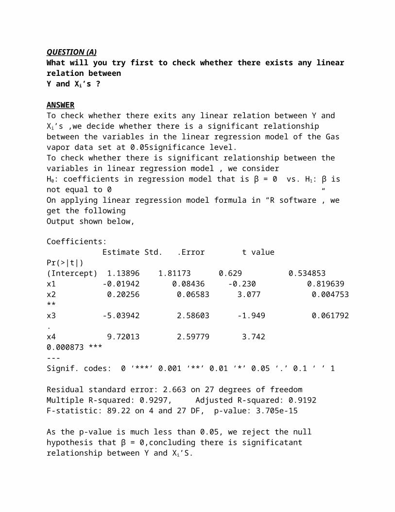
QUESTION (A)What will you try first to check whether there exists any linear relation betweenY and Xi’s ?

ANSWERTo check whether there exits any linear relation between Y and Xi’s ,we decide whether there is a significant relationship between the variables in the linear regression model of the Gas vapor data set at 0.05significance level.To check whether there is significant relationship between the variables in linear regression model , we consider H0: coefficients in regression model that is β = 0 vs. H1: β is not equal to 0On applying linear regression model formula in “R software”, we get the following Output shown below,

Coefficients: Estimate Std. .Error t value Pr(>|t|) (Intercept) 1.13896 1.81173 0.629 0.534853 x1 -0.01942 0.08436 -0.230 0.819639 x2 0.20256 0.06583 3.077 0.004753** x3 -5.03942 2.58603 -1.949 0.061792. x4 9.72013 2.59779 3.742 0.000873 ***---Signif. codes: 0 ‘***’ 0.001 ‘**’ 0.01 ‘*’ 0.05 ‘.’ 0.1 ‘ ’ 1

Residual standard error: 2.663 on 27 degrees of freedomMultiple R-squared: 0.9297, Adjusted R-squared: 0.9192 F-statistic: 89.22 on 4 and 27 DF, p-value: 3.705e-15

As the p-value is much less than 0.05, we reject the null hypothesis that β = 0,concluding there is significatant relationship between Y and Xi’S.

Now,our second approach is Graphics displays of relationship between observed values “Y” and predictor variables “Xi’s”. T hisis just a two-dimensional array of two dimensionalplots,where(except for the diagonal) each frame contains a scatter diagram.Thus,each plot is an attempt to shed light on the relationship between a pair of variables, which gives a sense of linearity or non linearity of the relationship and some awareness of how the individual data points are arrangedover the region.If data points are symmetrically scattered arounddiagonal line in graph panel ,we can sense there is linear relationship between observed “Y”and predictor variables “XI’S”.

Graphical display is shown among observed “Y”and predictor variables “XI’S”

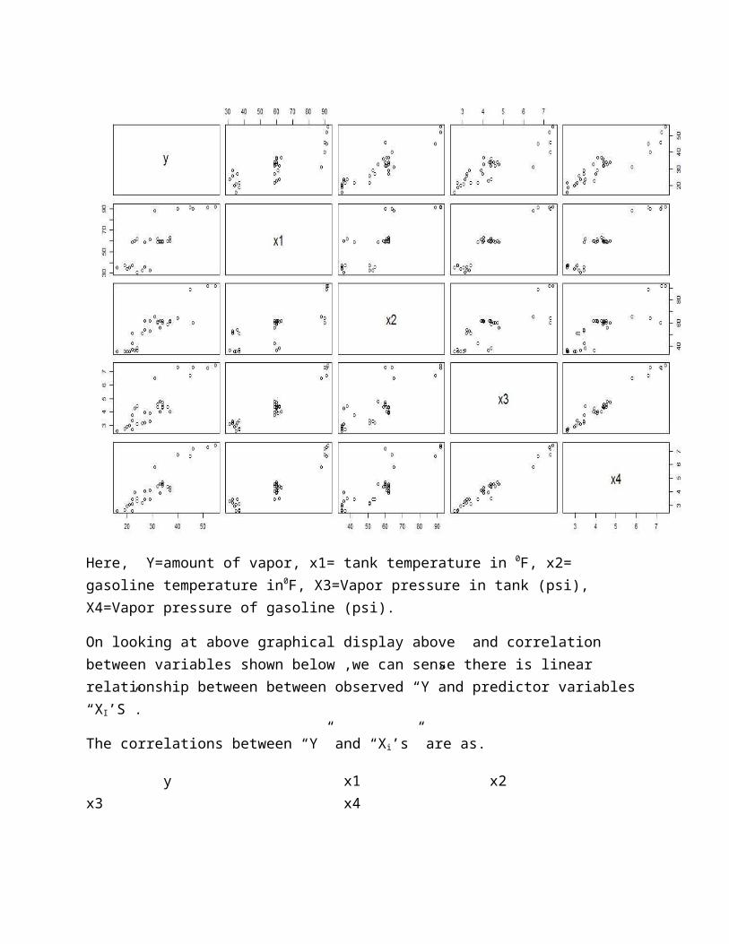
Here, Y=amount of vapor, x1= tank temperature in 0F, x2= gasoline temperature in0F, X3=Vapor pressure in tank (psi), X4=Vapor pressure of gasoline (psi).

On looking at above graphical display above and correlation between variables shown below ,we can sense there is linear relationship between between observed “Y”and predictor variables “XI’S”.

The correlations between “Y” and “Xi’s” are as. y x1 x2 x3 x4

y 1.0000000 0.8260665 0.9093507 0.8650301 0.9213333.

QUESTION(B)

Suppose “y” depends on all the “Xi’s” in linear fashion ,find thebest possible prediction equation based on data .

ANSWER

On applying linear regression model to gas vapor datasets,

We get coefficients terms for intercept and predictor variables as

(Intercept) x1 x2 x3 x4

1.13896410 -0.01942314 0.20256230 -5.03942079 9.72013344

Therefore our best possible prediction equation based on assumption of “y” depends on all the “Xi’s” in linear fashion is,

Y=1.13896410 -0.01942314 X1+0.20256230 X2 -5.03942079X3+9.72013344 X4.

With Multiple R-squared: 0.9297, The coefficient of determination R2 is a measure of the global fit of the model. Specifically, R2 is an element of [0, 1] and represents the proportion of variability in Y that may be attributed to some linear combination of the predictors in Xi’s.

QUESTION(C) Find the confidence band for each of the parameters.

ANSWER

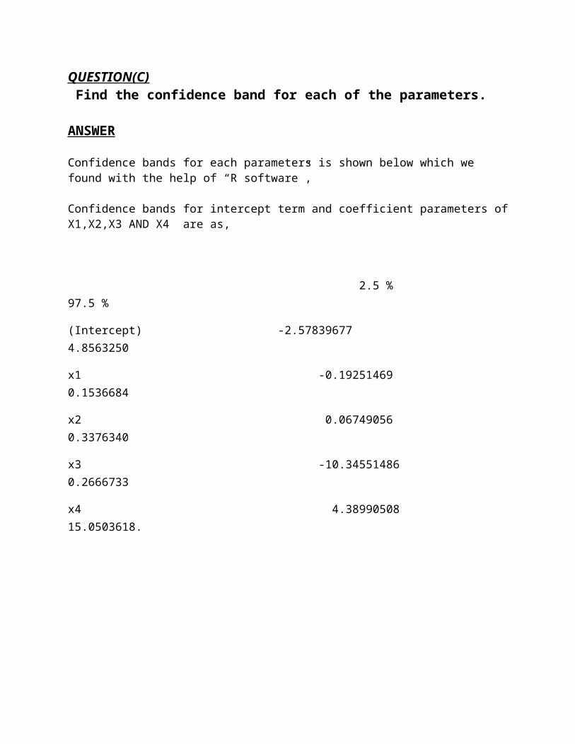
Confidence bands for each parameters is shown below which we found with the help of “R software”,

Confidence bands for intercept term and coefficient parameters ofX1,X2,X3 AND X4 are as,

2.5 % 97.5 %

(Intercept) -2.57839677 4.8563250

x1 -0.19251469 0.1536684

x2 0.06749056 0.3376340

x3 -10.34551486 0.2666733

x4 4.38990508 15.0503618.

QUSTION(D)State the model assumptions you are making to obtain (b) and (c) and verify whether they are satisfying or no.

ANSWERThe following assumptions that I have made in order to obtain (b)and(c) are as follows:

1) The relationship between the “ Y” and the “Xis” is linear,atleast approximately.

2) The error term has constant variance.3) The errors are uncorrelated.4) The errors are normally distributed.

Verifications:

1) The relationship between the “ Y” and the “Xis” is linear,atleast approximately.

I have already shown above in question (a), that the relationship between “Y “ and the “Xi’s” is linear.

2) The error term has constant variance

We use score test also known as “BREUSCH-PAGAN TEST” for non constant “error” variance test,For which we computes a score test of the null hypothesis of constant error variance against the alternative that the error variance changes with the level ofthe response (fitted values), or with a linear combination of predictors.

Null hypothesis: error term has constant variance

Atlternative hypothesis: error term has not constant variance.

Non-constant Variance Score Test

Variance formula: ~ fitted.values

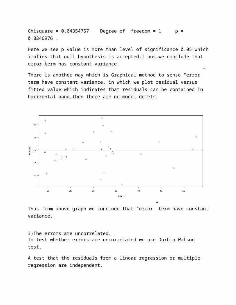
Chisquare = 0.04354757 Degree of freedom = 1 p = 0.8346976 .

Here we see p value is more than level of significance 0.05 whichimplies that null hypothesis is accepted.T hus,we conclude that error term has constant variance.

There is another way which is Graphical method to sense “error” term have constant variance, in which we plot residual versus fitted value which indicates that residuals can be contained in horizontal band,then there are no model defets.

Thus from above graph we conclude that “error” term have constantvariance.

3)The errors are uncorrelated.To test whether errors are uncorrelated we use Durbin Watson test.

A test that the residuals from a linear regression or multiple regression are independent.

In this test, Darbin Watson statistic is applied to the residuals from least squares regressions, and developed bounds tests for the null hypothesis that the errors are serially uncorrelated against the alternative that they follow a first order autoregressive process.

Null hypothesis: errors are serially uncorrelated.

Alternative hypothesis: They follow a first order autoregressive process.Using “R software” we get darbin Watson test values as

lag Autocorrelation D-W Statistic p-value

1 -0.1772921 2.309197 0.354.

We see p-value is greater than level of significance 0.05 ,thus our null hypothesis that errors are serially uncorrelated is accepted.

4)The errors are normally distributed.

For this we plot QQ plot between standardized residuals and normal scores in order to conclude errors are normally distributed.

http://en.wikipedia.org/wiki/Autoregressive

http://en.wikipedia.org/wiki/Null_hypothesis

http://en.wikipedia.org/wiki/Ordinary_least_squares

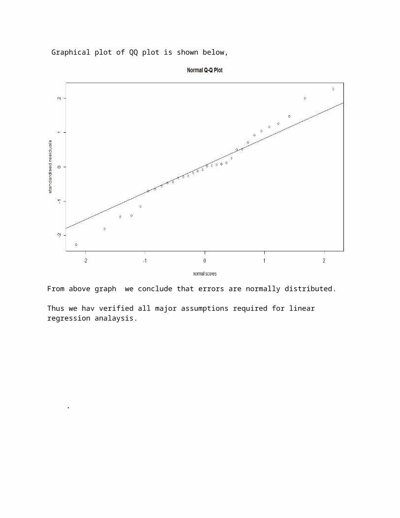
Graphical plot of QQ plot is shown below,

From above graph we conclude that errors are normally distributed.

Thus we hav verified all major assumptions required for linear regression analaysis.

.

QUESTION(E)

Find the best possible model using AIC approach.

ANSWER

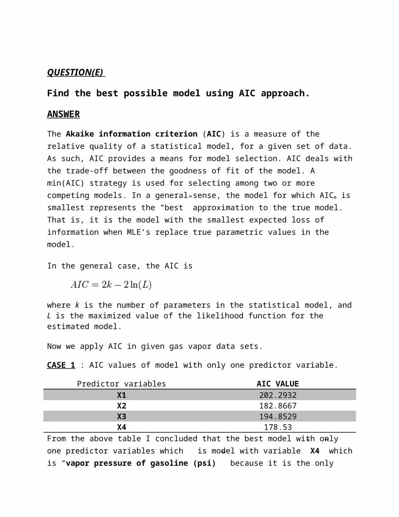
The Akaike information criterion (AIC) is a measure of the relative quality of a statistical model, for a given set of data.As such, AIC provides a means for model selection. AIC deals withthe trade-off between the goodness of fit of the model. A min(AIC) strategy is used for selecting among two or more competing models. In a general sense, the model for which AICm issmallest represents the “best” approximation to the true model. That is, it is the model with the smallest expected loss of information when MLE’s replace true parametric values in the model.

In the general case, the AIC is

where k is the number of parameters in the statistical model, andL is the maximized value of the likelihood function for the estimated model.

Now we apply AIC in given gas vapor data sets.

CASE 1 : AIC values of model with only one predictor variable.

Predictor variables AIC VALUEX1 202.2932X2 182.8667X3 194.8529X4 178.53

From the above table I concluded that the best model with only one predictor variables which is model with variable” X4” whichis “vapor pressure of gasoline (psi)” because it is the only

http://en.wikipedia.org/wiki/Likelihood_function

http://en.wikipedia.org/wiki/Statistical_model

http://en.wikipedia.org/wiki/Parameter

http://en.wikipedia.org/wiki/Goodness_of_fit

http://en.wikipedia.org/wiki/Statistical_model

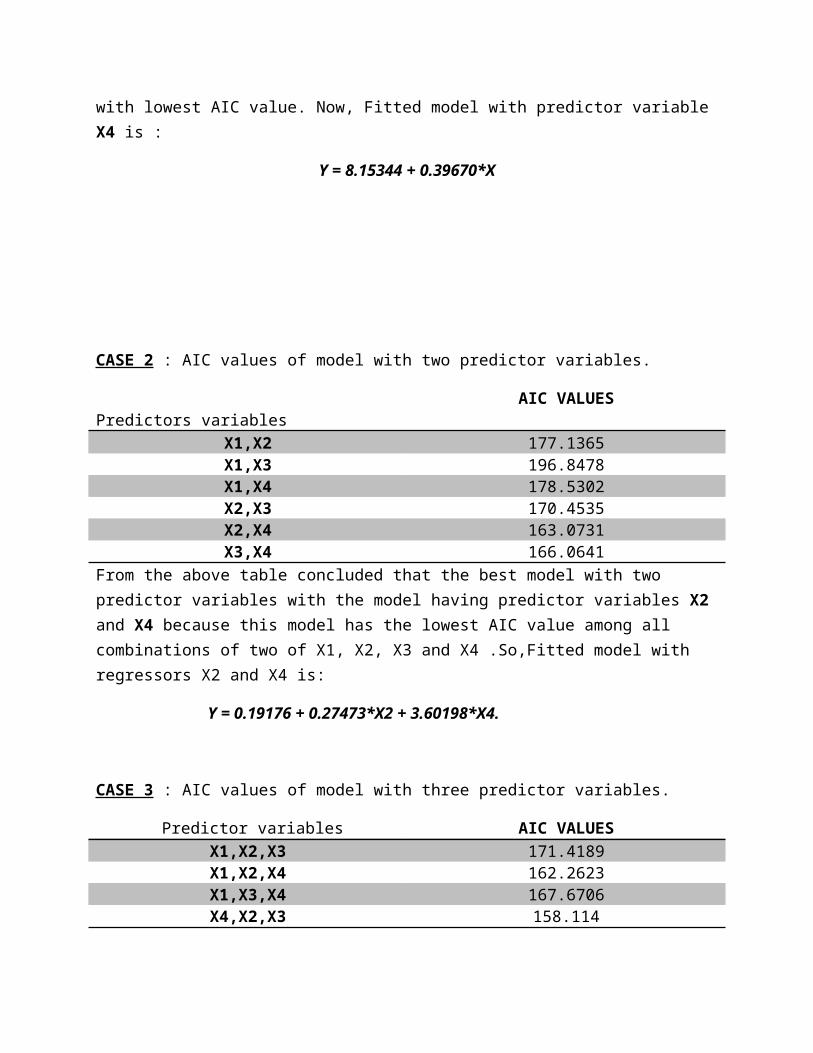
with lowest AIC value. Now, Fitted model with predictor variable X4 is :

Y = 8.15344 + 0.39670*X

CASE 2 : AIC values of model with two predictor variables.

Predictors variables

AIC VALUES

X1,X2 177.1365X1,X3 196.8478X1,X4 178.5302X2,X3 170.4535X2,X4 163.0731X3,X4 166.0641

From the above table concluded that the best model with two predictor variables with the model having predictor variables X2 and X4 because this model has the lowest AIC value among all combinations of two of X1, X2, X3 and X4 .So,Fitted model with regressors X2 and X4 is:

Y = 0.19176 + 0.27473*X2 + 3.60198*X4.

CASE 3 : AIC values of model with three predictor variables.

Predictor variables AIC VALUESX1,X2,X3 171.4189X1,X2,X4 162.2623X1,X3,X4 167.6706X4,X2,X3 158.114

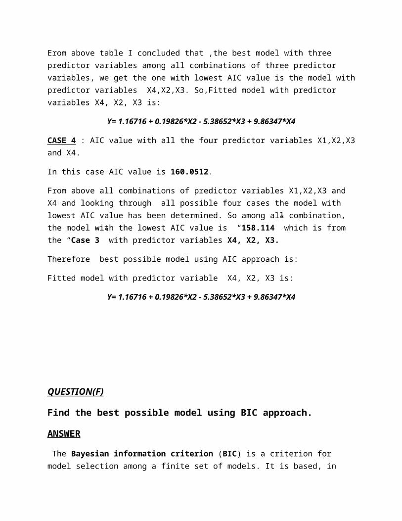
Erom above table I concluded that ,the best model with three predictor variables among all combinations of three predictor variables, we get the one with lowest AIC value is the model withpredictor variables X4,X2,X3. So,Fitted model with predictor variables X4, X2, X3 is:

Y= 1.16716 + 0.19826*X2 - 5.38652*X3 + 9.86347*X4

CASE 4 : AIC value with all the four predictor variables X1,X2,X3and X4.

In this case AIC value is 160.0512.

From above all combinations of predictor variables X1,X2,X3 and X4 and looking through all possible four cases the model with lowest AIC value has been determined. So among all combination, the model with the lowest AIC value is “158.114” which is from the “Case 3” with predictor variables X4, X2, X3.

Therefore best possible model using AIC approach is:

Fitted model with predictor variable X4, X2, X3 is:

Y= 1.16716 + 0.19826*X2 - 5.38652*X3 + 9.86347*X4

QUESTION(F)

Find the best possible model using BIC approach.

ANSWER

The Bayesian information criterion (BIC) is a criterion for model selection among a finite set of models. It is based, in

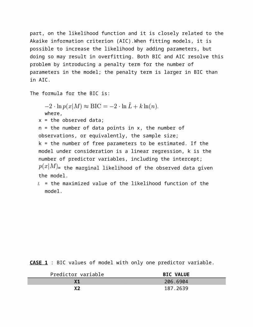
http://en.wikipedia.org/wiki/Model_selection

part, on the likelihood function and it is closely related to theAkaike information criterion (AIC).When fitting models, it is possible to increase the likelihood by adding parameters, but doing so may result in overfitting. Both BIC and AIC resolve thisproblem by introducing a penalty term for the number of parameters in the model; the penalty term is larger in BIC than in AIC.

The formula for the BIC is:

where,x = the observed data;n = the number of data points in x, the number of observations, or equivalently, the sample size;k = the number of free parameters to be estimated. If the model under consideration is a linear regression, k is the number of predictor variables, including the intercept;

= the marginal likelihood of the observed data given the model.

= the maximized value of the likelihood function of the model.

CASE 1 : BIC values of model with only one predictor variable.

Predictor variable BIC VALUEX1 206.6904X2 187.2639


http://en.wikipedia.org/wiki/Marginal_likelihood

http://en.wikipedia.org/wiki/Overfitting

http://en.wikipedia.org/wiki/Akaike_information_criterion


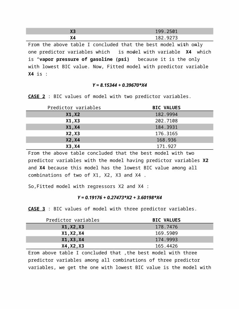
X3 199.2501X4 182.9273

From the above table I concluded that the best model with only one predictor variables which is model with variable” X4” whichis “vapor pressure of gasoline (psi)” because it is the only with lowest BIC value. Now, Fitted model with predictor variable X4 is :

Y = 8.15344 + 0.39670*X4

CASE 2 : BIC values of model with two predictor variables.

Predictor variables BIC VALUESX1,X2 182.9994X1,X3 202.7108X1,X4 184.3931X2,X3 176.3165X2,X4 168.936X3,X4 171.927

From the above table concluded that the best model with two predictor variables with the model having predictor variables X2 and X4 because this model has the lowest BIC value among all combinations of two of X1, X2, X3 and X4 .

So,Fitted model with regressors X2 and X4 :

Y = 0.19176 + 0.27473*X2 + 3.60198*X4

CASE 3 : BIC values of model with three predictor variables.

Predictor variables BIC VALUESX1,X2,X3 178.7476X1,X2,X4 169.5909X1,X3,X4 174.9993X4,X2,X3 165.4426

Erom above table I concluded that ,the best model with three predictor variables among all combinations of three predictor variables, we get the one with lowest BIC value is the model with

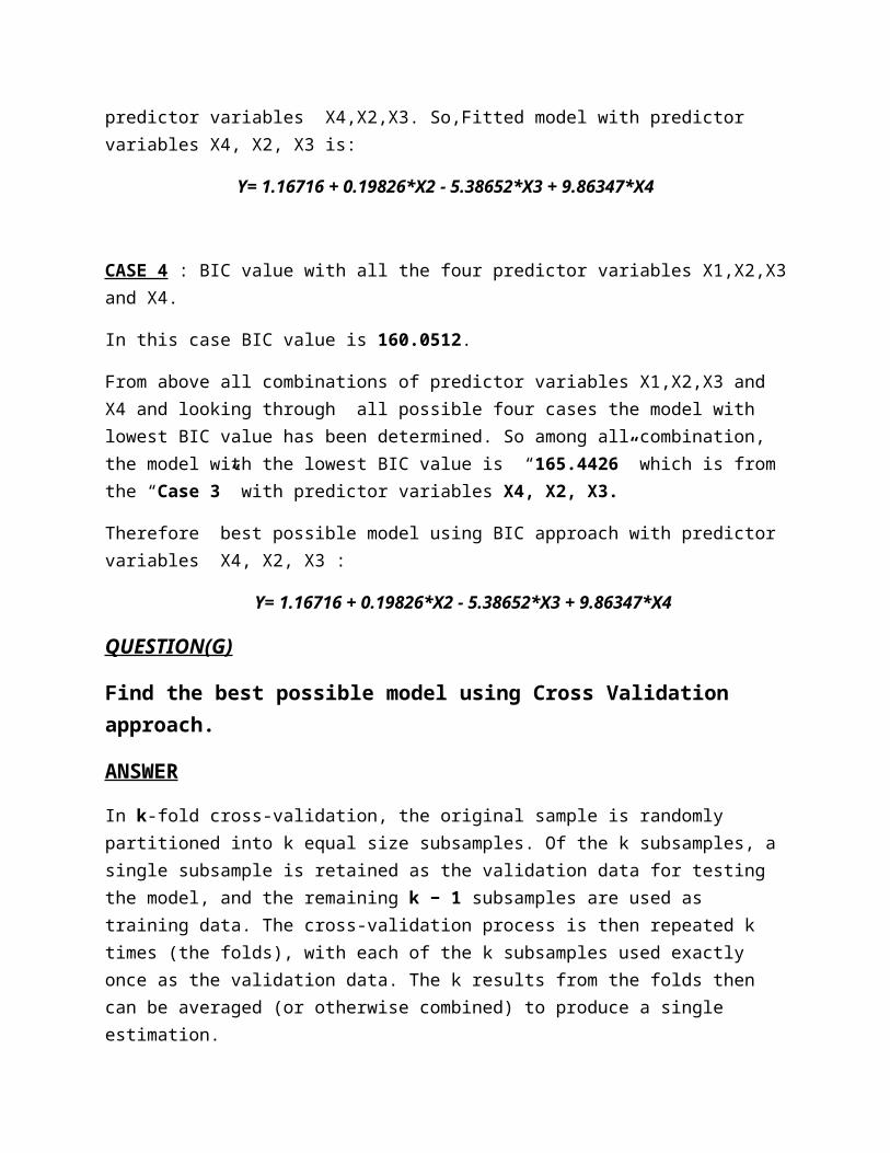
predictor variables X4,X2,X3. So,Fitted model with predictor variables X4, X2, X3 is:

Y= 1.16716 + 0.19826*X2 - 5.38652*X3 + 9.86347*X4

CASE 4 : BIC value with all the four predictor variables X1,X2,X3and X4.

In this case BIC value is 160.0512.

From above all combinations of predictor variables X1,X2,X3 and X4 and looking through all possible four cases the model with lowest BIC value has been determined. So among all combination, the model with the lowest BIC value is “165.4426” which is from the “Case 3” with predictor variables X4, X2, X3.

Therefore best possible model using BIC approach with predictor variables X4, X2, X3 :

Y= 1.16716 + 0.19826*X2 - 5.38652*X3 + 9.86347*X4

QUESTION(G)

Find the best possible model using Cross Validation approach.

ANSWER

In k-fold cross-validation, the original sample is randomly partitioned into k equal size subsamples. Of the k subsamples, a single subsample is retained as the validation data for testing the model, and the remaining k − 1 subsamples are used as training data. The cross-validation process is then repeated k times (the folds), with each of the k subsamples used exactly once as the validation data. The k results from the folds then can be averaged (or otherwise combined) to produce a single estimation.

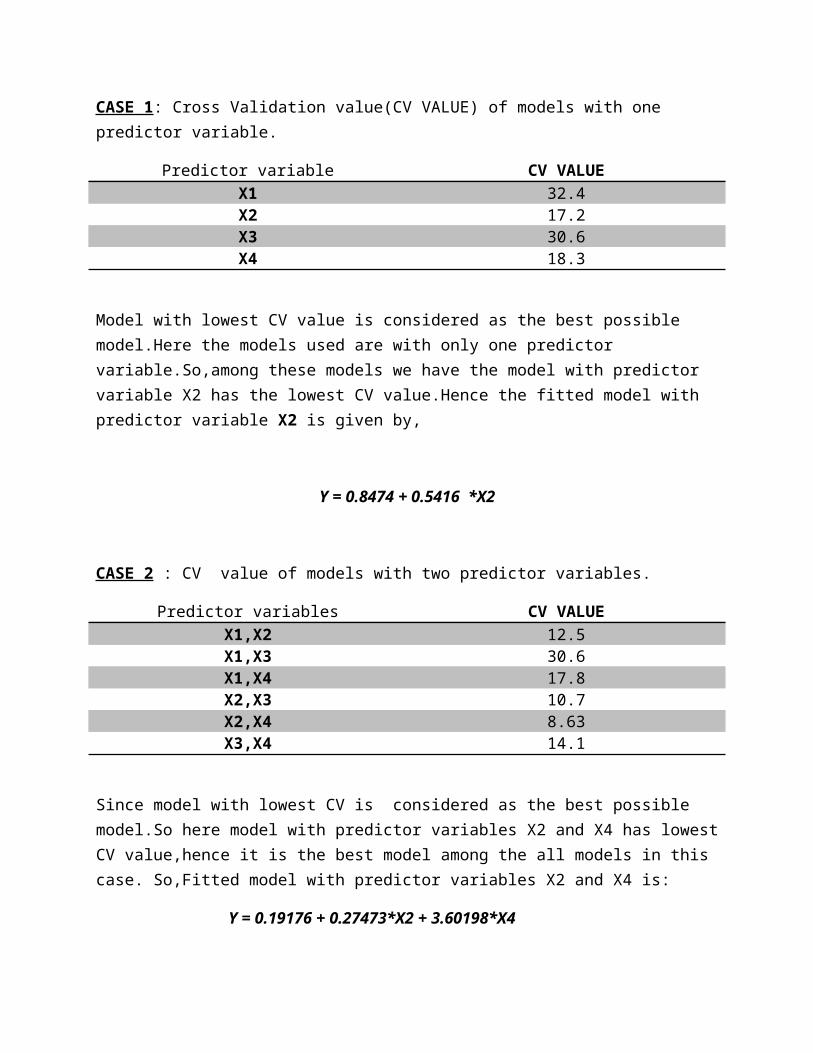
CASE 1: Cross Validation value(CV VALUE) of models with one predictor variable.

Predictor variable CV VALUEX1 32.4X2 17.2X3 30.6X4 18.3

Model with lowest CV value is considered as the best possible model.Here the models used are with only one predictor variable.So,among these models we have the model with predictor variable X2 has the lowest CV value.Hence the fitted model with predictor variable X2 is given by,

Y = 0.8474 + 0.5416 *X2

CASE 2 : CV value of models with two predictor variables.

Predictor variables CV VALUEX1,X2 12.5X1,X3 30.6X1,X4 17.8X2,X3 10.7X2,X4 8.63X3,X4 14.1

Since model with lowest CV is considered as the best possible model.So here model with predictor variables X2 and X4 has lowestCV value,hence it is the best model among the all models in this case. So,Fitted model with predictor variables X2 and X4 is:

Y = 0.19176 + 0.27473*X2 + 3.60198*X4

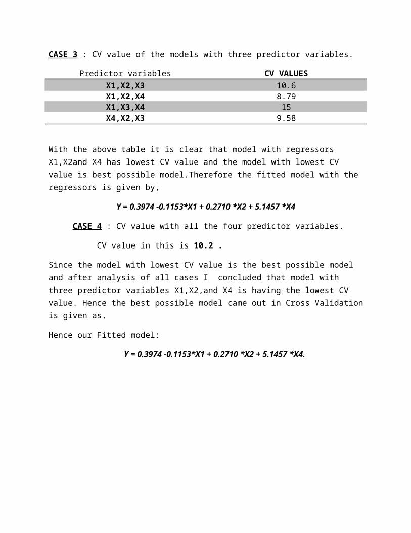
CASE 3 : CV value of the models with three predictor variables.

Predictor variables CV VALUESX1,X2,X3 10.6X1,X2,X4 8.79X1,X3,X4 15X4,X2,X3 9.58

With the above table it is clear that model with regressors X1,X2and X4 has lowest CV value and the model with lowest CV value is best possible model.Therefore the fitted model with the regressors is given by,

Y = 0.3974 -0.1153*X1 + 0.2710 *X2 + 5.1457 *X4

CASE 4 : CV value with all the four predictor variables.

CV value in this is 10.2 .

Since the model with lowest CV value is the best possible model and after analysis of all cases I concluded that model with three predictor variables X1,X2,and X4 is having the lowest CV value. Hence the best possible model came out in Cross Validationis given as,

Hence our Fitted model:

Y = 0.3974 -0.1153*X1 + 0.2710 *X2 + 5.1457 *X4.

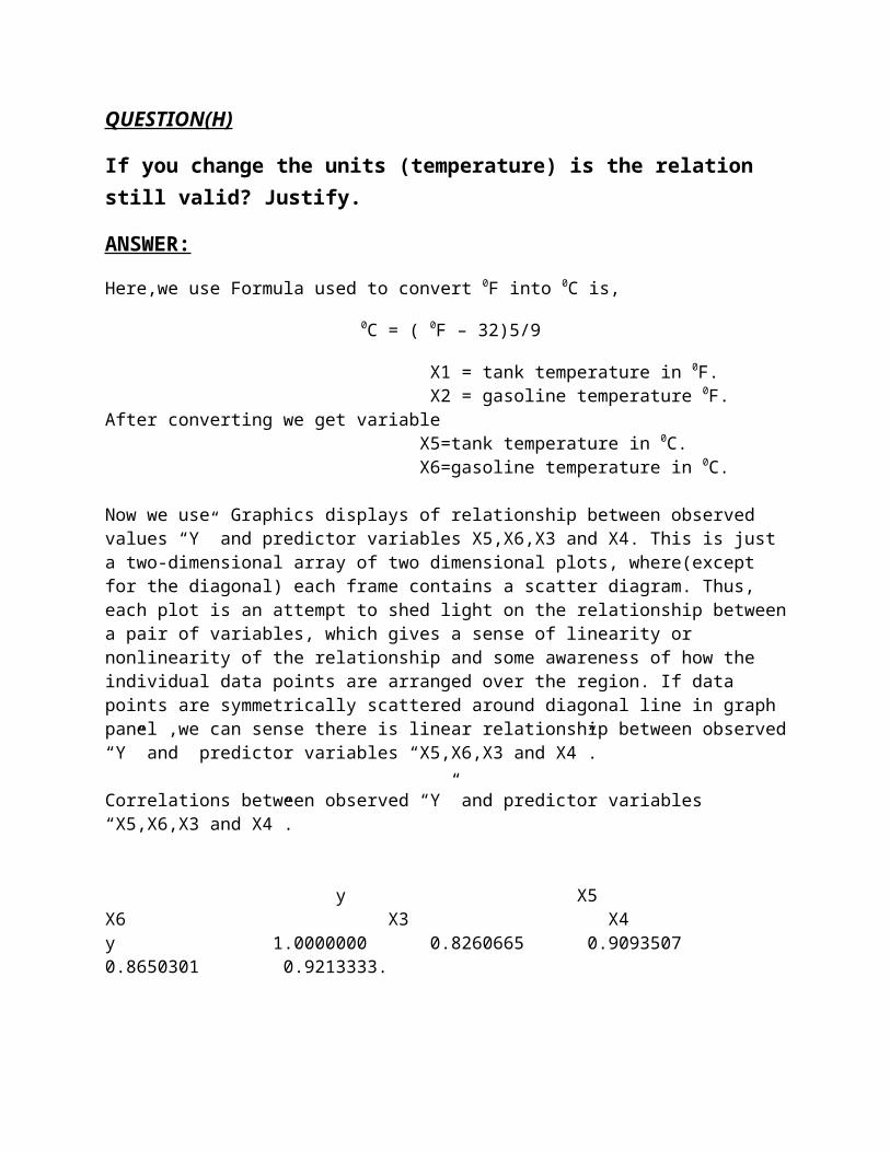
QUESTION(H)

If you change the units (temperature) is the relation still valid? Justify.

ANSWER:

Here,we use Formula used to convert 0F into 0C is,

0C = ( 0F – 32)5/9

X1 = tank temperature in 0F. X2 = gasoline temperature 0F.After converting we get variable X5=tank temperature in 0C. X6=gasoline temperature in 0C.

Now we use Graphics displays of relationship between observed values “Y” and predictor variables X5,X6,X3 and X4. This is just a two-dimensional array of two dimensional plots, where(except for the diagonal) each frame contains a scatter diagram. Thus, each plot is an attempt to shed light on the relationship betweena pair of variables, which gives a sense of linearity or nonlinearity of the relationship and some awareness of how the individual data points are arranged over the region. If data points are symmetrically scattered around diagonal line in graph panel ,we can sense there is linear relationship between observed“Y” and predictor variables “X5,X6,X3 and X4”.

Correlations between observed “Y” and predictor variables “X5,X6,X3 and X4”.

y X5 X6 X3 X4y 1.0000000 0.8260665 0.9093507 0.8650301 0.9213333.

Here, Y=amount of vapor, x5= tank temperature in 0C, x2= gasoline temperature in0C, X3=Vapor pressure in tank (psi), X4=Vapor pressure of gasoline (psi).

On looking at graphical display shown below of relationship between observed variable “Y”and predictor variables “X5,X6,X3 and X4” and high correlations between “Y”and predictor variables “X5,X6,X3 and X4”,shows there still exits linear relationship between “Y”and predictor variables “X5,X6,X3 and X4”.

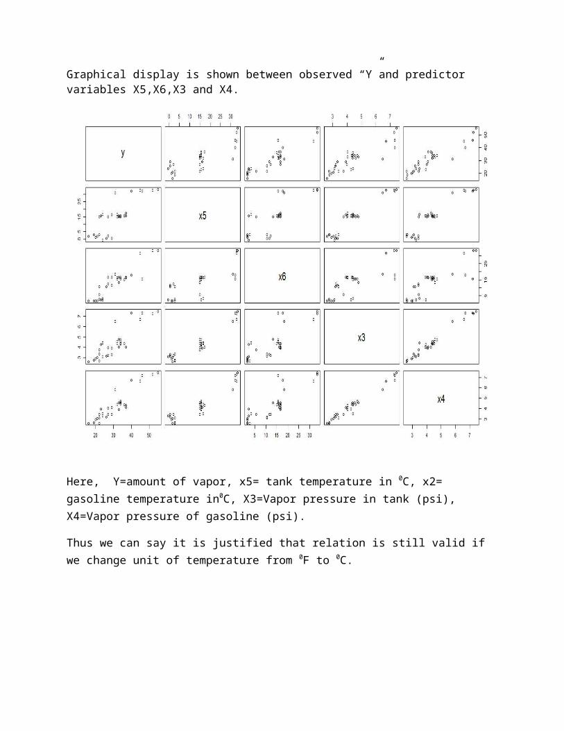
Graphical display is shown between observed “Y”and predictor variables X5,X6,X3 and X4.

Here, Y=amount of vapor, x5= tank temperature in 0C, x2= gasoline temperature in0C, X3=Vapor pressure in tank (psi), X4=Vapor pressure of gasoline (psi).

Thus we can say it is justified that relation is still valid if we change unit of temperature from 0F to 0C.

Appendix:

Here we used “R 3.0.1 software” and packages for regression analysis of given gas vapor data sets.

Pacakages include “DAAG”, “car”, and “MASS”.

plot(gasvapor) code for scatterplot matrix

cor(gasvapor) code for correlation between Y and Xi’s

gas.fit=lm(y~x1+x2+x3+x4,data=gasvapor) code for fitting of model

confint(gas.fit,level=0.95 ) code for confidence band

ncvTest(fit) code for showing error term has constant variance.

q<-gas.fit$fitted code forgetting fitted value form fitting model

zx<-gas.fit$residuals code for getting residuals value form fitting model

Plot(q,zx) code for plotting residual vs. fitted value. abline(h=0,lwd=2)

durbinWatsonTest(fi code for showing errors are uncorrelated.

code for showing error term is normally distributed

zx1<-rstandard(gas.fit)

> qqnorm(zx1,ylab="standardised residuals",xlab="normal scores")

> qqline(zx1)

code used for AIC approach

gasfit1=lm(y~x1,data=gasvapor)

AIC(gasfit1)


AIC(gasfit2)


AIC(gasfit3)


AIC(gasfit4)

gasfit2.1=lm(y~x1+x2,data=gasvapor)

AIC(gasfit2.1)


AIC(gasfit2.2)


AIC(gasfit2.3)


AIC(gasfit2.4)


AIC(gasfit2.5)


AIC(gasfit2.6)

gasfit3.1=lm(y~x1+x2+x3,data=gasvapor)

AIC(gasfit3.1)


AIC(gasfit3.2)


AIC(gasfit3.3)


AIC(gasfit3.4)

AIC(gas.fit)

code used for BIC approach

BIC(gas.fit)

BIC(gasfit1)

BIC(gasfit2)

BIC(gasfit3)

BIC(gasfit4)

BIC(gasfit2.1)

BIC(gasfit2.2)

BIC(gasfit2.3)

BIC(gasfit2.4)

BIC(gasfit2.5)

BIC(gasfit2.6)

BIC(gasfit3.1)

BIC(gasfit3.2)

BIC(gasfit3.3)

BIC(gasfit3.4)

code used for Cross Validation

cv1.1=CVlm(df=gasvapor,form.lm=formula(y~x1))




cv2.1=CVlm(df=gasvapor,form.lm=formula(y~x1+x2))






cv3.1=CVlm(df=gasvapor,form.lm=formula(y~x1+x2+x3))




cv4.0=CVlm(df=gasvapor,form.lm=formula(y~x1+x2+x3+x4))

code for converting 0F into 0C

X5=5*(x1-32)/9

X6=5*(x2-32)/9

code for Changed after unit conversion dataset into data frame

gasvapor1=data.frame(y,x5,x6,x3,x4)

code for checking relationship in part (h)

plot(gasvapor1)

cor(gasvapor1)

regression project 1

Documents

Transcript of regression project 1