Multiple scale finite element methods

INTERNATIONAL JOURNAL FOR NUMERICAL METHODS IN ENGINEERING, VOL. 32,969-990 (1991)

MULTIPLE SCALE FINITE ELEMENT METHODS *

WING KAM LIU,' YAN ZHANG' AND MARTIN R. RAMIREZG

Northwestern University, Department of Mechanical Engineering, Evanston, IL 60208, U.S.A.

SUMMARY New temporal and spatial discretization methods are developed for multiple scale structural dynamic problems. The concept of fast and slow time scales is introduced for the temporal discretization. The required time step is shown to be dependent only on the slow time scale, and therefore, large time steps can be used for high frequency problems. To satisfy the spatial counterpart of the requirement on time step constraint, finite-spectral elements and finite wave elements are developed. Finite-spectral element methods combine the usual finite elements with the fast convergent spectral functions to obtain a faster convergence rate; whereas, finite wave elements are developed in parallel to the temporal shifting technique. Therefore, the spatial resolution is increased substantially. These methods are especially applicable to structural acoustics and linear space structures. Numerical examples are presented to illustrate the effectiveness of these methods.

1. INTRODUCTION

Traditionally, researchers in computational analysis have concentrated on bringing more detail into their structural system models, but have ignored the multi-time and multi-spatial scales inherent in the structural response. To obtain resolution of medium frequencies, finite element meshes consisting of several thousand structural and continuum elements are necessary. To resolve the time scale problem, either a very small integration time step is required or if modal superposition is used, a large number of structural eigenmodes is needed. These solutions often require hours of computer time on even the latest supercomputers. This severely limits the usefulness of these computations since their use in the design process is almost impossible.

Conversely, researchers in structural design and analysis have concentrated on the modelling of various structural components, usually via lumped parameters, but have often used drastic simplifications so that the multi-scale problem is eliminated. The accuracy of these methods is limited to the very low end of the spectrum, however.

There are two basic types of methods for dealing with transient structural dynamics problems: (1) modal superposition, and (2) direct integration. In modal superposition methods, the structural dynamics equations or matrix equations of motion are diagonalized by using the eigenvalues and eigenvectors. These eigenvalues and eigenvectors correspond to the natural frequencies and modes. In direct integration, the matrix equations are integrated using a numerical step-by-step procedure without transformation of the equations. In linear analysis, the

*The support of this research by the ONR Contract N00014-87-K-0756 and the NSF Grant EET-8806347 is gratefully acknowledged + Professor *Graduate assistant Currently Asst. Professor, The Johns Hopkins University, Department of Civil Engineering, Baltimore, MD 21218, USA

0029-598 1 /9 1 / 130969-22$11 .OO 0 1991 by John Wiley & Sons, Ltd.

Received 25 May 1990 Revised 19 September I990

970 W. K. LIU, Y. ZHANG AND M. R. RAMIREZ

choice of method depends on the frequency content of the response and on which portion of the frequency response is of interest.

In modal superposition procedures, the most critical and time-consuming aspect of the computation is the determination of the eigenvalues and eigenvectors. There are a number of eigenvalue methods used in practice. 1,9 Methods such as vector iteration, Jacobi, Householder-QR-inverse iteration, subspace iteration, Rayleigh-Ritz reduction, Lanczos algorithms and reduced basis techniques are available. However, as higher values of frequencies are considered, owing to higher modal density, the extraction of eigenmodes can become very difficult and expensive. The modal equations of motion can be solved in closed form for linear combina- tions of simple loads. For a general loading, computation becomes quite lengthy.

Direct time integration methods play an important role in the computer simulation of linear and non-linear problems. Basically, there are two general classes of direct integration methods: (1) implicit integration, and (2) explicit i n t eg ra t i~n .~ .~ Both methods are developed from difference formulas that relate the accelerations, velocities and displacements. Implicit algorithms, some of which are unconditionally stable, permit large time steps, but the cost per step is high and storage requirements tend to increase dramatically with the size of the mesh. On the other hand, explicit algorithms, which are conditionally stable, tend to be inexpensive per step and require less storage than implicit algorithms; but numerical stability requires the size of the time step to be inversely proportional to the highest frequency of the finite element mesh so they are quite ineffective for the study of long-duration response in the medium frequency range. Hybrid methods, such as implicit-explicit nodal partitions, implicit-explicit mesh partitions, staggered solution procedures, mixed-time integration, and unconditionally stable explicit and implicit-explicit time integration algorithms2"0, 11, 13-17 ,26 h ave been proposed to improve the efficiency of direct time integrations. For a complete review of these methods, see Reference 3.

In the high frequency end, methods which in this paper are referred to as asymptotic methods, such as ray methods,' asymptotic expansions,' WKBJ approximation,'8 method of averaging,'* subspace projection method^,^*^,'^ etc., are sufficient to accurately predict the response. In the low frequency spectrum, methods which in this paper are referred to as structural dynamics methods, such as implicit time integration, modal analysis, and reduced basis techniques, are suitable.

Some methods, such as matched asymptotic expansions, methods of multiple scales, primary and secondary systems approaches,12, 21,25 and matching asymptotic and structural dynamics methods," have been proposed to simultaneously achieve the attributes of both asymptotic methods and structural dynamics methods. Most of these methods are aimed at special classes of problems, and in most situations they are not applicable to complex structures. Furthermore, the engineering literature in this area is quite limited, and little success has been reported in structural dynamics applications.

In multiple scale problems of linear structures, tbe response can be viewed as a superposition of components with a wide frequency spectrum. Therefore, both structural dynamics methods and asymptotic methods are not efficient for this type of problem. In this paper, these difficulties are overcome by decomposing the response into fast and slow time scales using temporal shifting. The slow time scale is solved by the direct time integration method with a reasonably large time step. The total response is then recovered via the sampling theorem and superposition. The temporal shifting technique has been implemented in other works for medium frequency problem^.^^,^^ As higher frequencies are being sampled the mesh needs to be augmented in its ability to resolve higher wave numbers, thus finite-spectral elements and finite wave elements are developed.

MULTIPLE SCALE FINITE ELEMENT METHODS 971

In Section 2, motivation and preliminaries of the proposed methods are presented. In Section 3, the new weak form for the dynamic analysis of the multiple scale problems is formulated. The medium frequency response is first decomposed into two scales, a fast time scale and a slow time scale. The solution of the slow time scale and recovery of the response are then outlined. The finite-spectral element formulation which employs the standard finite element shape functions and the modified spectral functions is presented in Section 4. The finite wave element formulation is then given in Section 5. Finally, some numerical examples are discussed in Section 6.

2. MOTIVATION AND PRELIMINARIES

In direct time integration of a linear structural dynamics problem, the time step can be determined by the accuracy required in the highest frequency of i n t e r e ~ t . ~ , ~ , ~ * ' ~ * ~ ~ Using the highest frequency to set the time step leads traditional structural dynamics methods to be quite inefficient for higher frequencies. In a different respect, modal analysis methods become intract- able for problems having high modal density.

It is highly desirable to solve the dynamic response in a selected frequency band effectively for computational economy. A further consideration from an engineering standpoint is that the response is sometimes needed within a particular frequency range only (usually in the medium frequency region) or a set of ranges. The response can then be obtained by the superposition of the solutions in several frequency bands.

The objective is to find uBr(x, t ) , a component of the displacement u(x, t), with the frequency content B, :

(1) B, = [rAo - Ao/2, rAo i- Ao/2] for r 3 112

where Aw and rAoi are the bandwidth and the centre of the band, respectively. The Fourier transform of uBr(x, t ) is

UBr(x, w) = U(x, w) for OE B, and UBr(x, o) = 0.0 for w#B, (2) where U(x, w) is the Fourier transform of u(x, t) .

uBr(x, t ) will be solved in the time domain directly. As r is often quite large in medium frequency problems, the finite element mesh must be sufficiently fine, i.e. the spatial counterpart of the requirement on time step refinement. Numerical methods need to be developed which are able to address the following issues:

(a) relaxation of time step constraints for the numerical integration; (b) satisfy spatial discretization requirements effectively by implementation of special elements.

To address issue (a), the frequency shifting and sampling techniques are employed to decom- pose the response into fast and slow scale components. The slow scale component uB(x, t ) has the frequency content

B = [ - Aw/2, A0/2] (3) The following steps are performed to obtain uB(x, t ) and then uBp(x, t ) :

1. Suppose the frequency content of u(x, t ) is shifted by rAw which results in a new function us(x, t) in the time domain as

u(x, t ) = eirAmtus(x, t ) (4)


where i = gives

- 1. To verify the above statement, using the shifting theorem6 in equation (3)

U(x, o) = utx, t)e-’@‘ddt = us(x, t)e”Aate-iat dt = U’(X,O - ~ A w ) (5) Ira I:w where U5(x, o) is the Fourier transform of us(x, t ) .

2, Two modified window functions w”t) and w B ( t ) of frequency bands and time steps -

B = ( [ - A - o/2 , Ahwj21, AF] and B = ([ - A o / 2 , A a / 2 ] , At> (6)

WE(,) = 1.0 €or W E B and WE(,) = 0.0 for w $ B (7)

are introduc~d, respectively. The choice of Am, Ahw, At and A t will depend on the type of application. The Fourier transform of wB(t ) , denoted by WB(o), has the usual property

and similarly for the window function wB(t ) . However, in numerical computation, us(x, t ) is first convolved with d ( t j in the time domain with a time step AF to obtain uBfx, t ) as

u”x, t ) = w”(t)**uS(x, t ) (8) According to the convolution theorem: u”x, t ) has the frequency band B.

sampled values of u E ( x , t ) by the sampling theorem: namely 3. The continuous function P(X, t j can be uniquely determined from knowledge of the

M

m = O P ( x , t ) = 2 us(,, mAt)wB(t - mAt) (9)

where M + 1 is the number of sampling points; and At is the sampling rate which satisfies the relation

2n At < - Ats

AW

Since wB has the frequency band B, aliasing will occur if equation (loa) is violated. Similarly, AF is chosen such that

AFG- At, m

and m is a real number. 4. The desired displacement component uBr(x, t ) is obtained as

uBrfx, t ) = Re(eirAufGs(x, t ) ) (1 1) where Re(z) recovers the real part of complex z. In the above equation, uBF(x, t) is decomposed into two time scales: a fast time scale eirAwt and a siow time scale P f x , t ) .

~ e ~ a ~ ~ ~ ~

1. In equation (91, as M goes to 00, Pfx, t ) approaches uBp(x, t). 2. The sampling theorem plays an important role in this study. As shown later, uBfx, mdt ) will

be solved only at selected discretized points, but UB(x, t> is available at any time t by equation (9), which makes the evaluation of uBr(x, t ) with a given frequency spectrum in equation (1 1) possible.

3. In steps 2 and 3, one can set B = B and obtain a simple formulation. But in this study, the


bandwidth A 0 is chosen such that A 0 2 Aw for reasons that will be discussed in the next section.

4. When these equations are used in the finite element analysis, some steps are carried out explicitly and some implicitly; therefore a new formulation of the FEM has emerged.

The medium frequency response can hardly be solved without addressing issue (b), because for this type of problem the finite element mesh often needs more spatial resolution than is readily provided by usual finite element methods. Two techniques are proposed in this paper. One is to use the usual finite element approximation in combination with higher order spectral functions. The key to the success of this spatial discretization is that the spectral functions satisfy homogeneous boundary conditions and that they are superimposed onto the finite element mesh which satisfies the essential boundary conditions. Another technique is to utilize the finite wave element. The shape functions of each element are constructed in relation to the centre of frequency band B,. They effectively span a subspace in which medium frequency response occurs.

3. FORMULATION OF MULTI-SCALE PROBLEMS

The weak form of the equations of motion can be written as

&(6u, 27) + V(6u, 2;) + X ( 6 u , u ) =/(Su, p ) (12) where A(., .), V(., .), Y(., .) and/(., .) are the usual mass, damping, stiffness and force assembly operators, respectively; 6u, u and p are the test function, trial function and forcing function, respectively; a superposed dot designates time differentiation.

The techniques introduced in the previous section are used. For each B, of interest, let

p(x, t ) = eirAwfps(x, t )

A S ( & , t i S ) + VS(6u, 22) + ,XS(6u, us) = f S ( B u , p S )

(13)

(14)

and substitute equations (4) and (13) into equation (12), yielding a new weak form

where

M y 62.4, 2) = A( 6u, tiS)

Vs(6u, 2;') = V(6u, 2) + 2irAwA(bu, 2;')

X s ( 6 u , us) = X ( 6 u , us) + irAwV(bu, u s ) - (rAw)' A ( 6 u , us) (15)

/"du, PSI =/(h pS)

To discretize equation (14) by the finite element approximation, the trial and test functions must be defined. The trial function is

Us(X, t ) = 1 NA(X, rAOJ)u>(t) (16) A

where NA( x, rAw) are the global shape functions (correspondingly, we employ lower case subscripts for element shape functions) which are dependent on the frequency content of B,; this will be discussed further in the next two sections. u>( t ) are the time varying nodal values. The test function is constructed as

974 W. K. LIU, Y. ZHANG A N D M. R. RAMIREZ

where 8uA(t ) are the nodal variations. Substituting equations (16) and (17) into equation (14) and then convolving both sides by the window function WE( t), gives the system of equations

(18) MSiS + CS&# + K S u & = pB

where Ms = [M>,] = A ( N A , N , )

Cs = [C>B] = %(&, N B ) f 2irAwk(NA, N B )

KS = [K>B] = X ( N A , NB) + irAw%(N,, NB) - (TAU)' A ( N A , A',)

= ( u Z ( t ) ) = {u>(t)**wB(t)) (19) UB = ( z i $ ( t ) } = (;>(tj**Wqt))

i iB = (ii!(t)} = {ii>(t)**wB(t))

PB = ( P $ ( t ) > =p(NA, p"t)**wB(t))

All matrices are still symmetric and banded. But some matrices are complex. Equation (18) can be solved by conventional implicit integration methods, such as the Newmark implicit method.

To obtain pB, the convolution of p"(t) and wB(t) is carried out effectively by using an FFT,4 whereas u>( t ) , t i>(t) and ii>(t) are automatically windowed in the direct time integration and sampled thereafter. According to equation (9), one has

M

m = O u B ( t ) z C uB(mAt)wB(t - mAt) (20)

where M is the total number of time steps used in integrating the slow time component. M + 1 is equal to the number of sampling points and At is defined in equation (10). It is noted that u B ( t ) is strictly in the frequency band B, as desired.

The reason for using a larger window, wB(t), in equation (19) than the response, wB(t), is that forcing components outside the frequency band B also contribute to the total response uB(t). The primary purpose of the present analysis is to obtain the response in the medium frequency band resulting from any loading which may significantly affect it. The bandwidths A 6 and Aw are arbitrary and can be set according to the problem characteristics or the response being sought. It is indeed possible to perform the converse operation to what is specifically addressed in this paper; setting A 6 < Aw will yield a broader response for a more specifically bandlimited loading. In arriving at a complete spectrum (all bands subjected to all bands in the loading) the results from the two approaches would be the same given the principle of superposition for linear structures. It is computationally feasible to do the present case using a large bandwidth for equation (19) since the time step need only be restricted to avoid aliasing and provide sufficient accuracy.

where m - 200.9 With uB(tj available at any time t from equation (20), uBr(t) is obtained as

uB'(t) = Re(eirAW'uB(t)) (221 In the steady-state case, equation (18) can be interpreted in the frequency domain. Applying the

Fourier transform to both sides of equation (18), the resulting equation is

HS(w)UB(~) = PB(w) (23)


where UB(o) and PB(w) are the Fourier transform of uB and pB respectively; )Is(@) is related to the familiar matrix transfer function, is given by

H”(w) = - w2Ms + ioCs + Ks (24)

uB( t ) is recovered by the inverse Fourier transformation:

[Hs(w)]-’PB(w)eim‘dw

However, it is not an easy task to evaluate equation (25), even though the integration i s performed only over 8, since [H”((w)l-’ has to be constructed for each w over B. With the exception of problems with low modal density, it is preferable to employ equation (18) in the time domain, instead of equation (25).

4. THE FINITE-SPECTRAL ELEMENTS FOR SPATIAL DISCRETIZATION

The essential and natural boundary conditions can easily be incorporated by the standard finite element shape functions and the convergence rate in the form of energy norm is obtained asz4

(26) X ( u - uh,u - Uh) < Ch2‘k-”’jlullk,

where u and uh are the exact and approximate solutions, respectively; h is the mesh size; 2m is the order of the differential equation; k - 1 is the degree of the shape function; C is a constant. To improve the approximation, one can refine the mesh h or increase the degree of the shape function k - 1. The latter approach is valuable for medium frequency problems, but appropriate higher order polynomials are not always easy to find. High order spectral functions have been observed to have a fast convergence rate, however, with some simple boundary conditions,’*’’ If the high order spectral functions are combined with the finite element shape functions, it may improve the convergence properties while retaining the flexibility of the finite element method. Based on this idea, the new element is developed by combining two sets of shape functions: a set of finite element shape functions which satisfy the required continuities; and another set of spectral functions which satisfy homogeneous boundary conditions. The trial function can then be expressed by

P 4

a = 1 a = 1 u ( t ) = C Na(x)ua(t) + t: Np+a(X)up+a(t) (27)

where N , ( x ) for a = 1, . . . , p are the usual finite element shape functions; N p + . ( x ) for a = 1, . . . , q are the spectral functions; ua( t ) are the generalized co-ordinates. The number of spectral functions q will depend on both the frequency band B, and the element size h. The element can be viewed as a higher order finite element; however, the convergence properties are much better than the classical h version having the same number of degrees of freedom, provided the appropriate spectral functions are employed. This approach has been studied in other works with different spectral f~nct ions.~

Well known for their fast convergence properties, Chebyshev polynomials are considered for constructing the spectral functions. The Chebyshev polynomial of degree n, denoted by q(l), is defined as (see Appendix I)

~ ( C O S 6 ) = cos(n6) (28)

976

thus,

W. K. LIU, Y. ZHANG A N D M. R. RAMIREZ

G(5) = 1

T(5) = 5 (29)

T,+,(5) = 251",(5) - 1"-1(t) for = 4 2 , . . . where 5 E [ - 1.0, 1.01. Two important properties of the Chebyshev polynomials are

T,( Jr 1) = ( Jr 1)n (30) and

The polynomials described above do not satisfy the homogeneous conditions at 5 = 2 1, so some manipulations are necessary upon the required continuities. Two important classes of the one dimensional element are developed in the natural co-ordinate system 5,

5 € [ - 1.0, 1.01

4.1. The C' finite-spectral element

element; they are also used here as the first set of shape functions, namely In the finite element method, Lagrange polynomials are often employed to form the Co

N a ( < ) = L,P-'(t) for a = 1, . . . , p (32) and

Lz- ' ( t )= fi (5 - < b ) / b = l fi b # a ( ( a - <a) (33) b = l b # a

where the 5, denote the locations of the nodes in the 5 co-ordinate system. In equation (33), p 2 2 is necessary to guarantee the continuity at the interfaces of the element.

The second set of shape functions is a series of spectral functions composed of the Chebyshev polynomials (see Appendix 11):

Equation (34a) satisfies the homogeneous conditions at the end points. That is,

N p + , ( t ) = 0.0 at 5 = t- 1 (35) which can be verified by equation (30).

As noted, the complete shape functions consist of two sets of independent polynomials. As spectral functions converge faster than Lagrange polynomials, it is recommended that only two linear Lagrange polynomials are used as the first set of shape functions to impose the continuity condition, that is


and the rest of the shape functions are the spectral functions as defined in equation (34) with p = 2.

Remarks:

1. For two or three dimensional problems, the elements can be constructed with the aid of one dimensional shape functions via the product rule, which is the standard technique in the finite element method.

2. The assembly procedure is quite similar to that of the element with internal nodes.

4.2. The C finite-spectral element

The C' shape functions are constructed in natural co-ordinates by imposing continuities, not only at the end points of the function, but also on its first derivative. The Hermite cubics are employed for the first set of shape functions, which gives

N , ( 5 ) = 1 - $( 1 + 5), + a( 1 + o3 N 3 ( 5 ) = ~ ( 1 + 5 ) 2 - $ ( 1 + 5 ) 3 N4(5)= - + ( 1 + 5 ) 2 + * ( 1 + 5 ) 3

N 2 ( 5 ) = ( 1 + 5) - (1 + 5 ) 2 +:(I + 51, (37)

where N , and N , are associated with the nodal value and its first derivative at 5 = - 1, and N , and N4 are associated with the nodal value and its first derivative at 5 = 1. The continuities at the end points are already guaranteed. The spectral functions have to be constructed so that their functions are derivatives vanish at the end points. Using the properties of the Chebyshev polynomials, let

and examining the boundary conditions at the end points by equations (30) and (31), one has

A complete higher order C' finite-spectral element is obtained by combining equations (37) and (38) (see Appendix 111).

5. FINITE WAVE ELEMENTS

The finite wave elements are developed based on the concept of frequency band solutions. As the response is sought for in a selected frequency band, it is desirable to construct a variational subspace which contains the appropriate wave number rAk, corresponding to the selected frequency band centred at rAo. The wave number k and the frequency o are generally related as

where c is the wave speed of the medium. Analogous to temporal shifting, which relaxes the time step restriction, the elements with spatial shifting are constructed so that the resolution of the spatial discretization will depend on the bandwidth Ak instead of the centre of the band rAk. In this paper, finite wave elements are presented for rod and beam elements. It should also provide some insight on the development of other structural and continuum elements.


5. I. The finite wave rod element

Wave propagation in an elastic rod is governed by the equation

82U(X, t) at2

= p A

where A, E and p are the area of cross-section, Young's modulus and density, respectively. The wave speed is -

c = J"- P

To establish us(x , t ) , rewrite equation (4) as

u(x, t) = eirAwtus(x, t) (43) Corresponding to the shift in time, spatial shifts are made which result in the finite wave element.

Considering the eth rod element, the trial function is written as

.. - where the shape functions are given by

and the nodal values lt; = (u:, u,)T

correspond to travelling waves in two directions. This element, in comparison with the usual linear rod element, has two degrees of freedom at

each node which account for the waves travelling in two directions; the shape functions and the nodal values are complex. Using the weak form of equation (41), the element mass and stiffness matrices for a rod can be constructed explicitly.

The eth element mass matrix is 1

[Mzb] = d" (N, , Nb) = A p (N,)TNbJdt for a, b = 1,2 (46) Il where J is

The eth element stiffness matrix can be written as

[KZb] = &'-"(No, Nb) = AE J: (2)T 2 J d t for a, b = 1,2

The element matrices are 4 x 4 symmetric and complex.

5.2. The finite wave element of a beam

The equation of motion of a beam is


where w(x, t) is the deflection of the beam and Z is the cross-section moment of inertia. The velocity of the wave is dependent on the frequency, therefore the bending beam is a dispersive medium:

Similarly, the finite wave element for a beam can be developed. The spatial discretization should be applied to ws( x, t ) with the corresponding spatial shift in wave number. Let

w(x, t ) = eirAwrws(x, t ) (51)

then the trial function for ws can be constructed around the wave number rAk. The general wave form in an elastic beam can be expressed in a linear combination of four terms: e-ikx, eikx, e-kx, and ekx. The last two exponential terms, having little effect in high frequency response, can be ignored. Therefore ws is expressed as

2

a = l w s = 1 NawS,

with

(534

i53b)

eirAkx N e-irAkx N eirAkx N, = [Nza-le-irAkx N2a- I > 2a 9 2a 1 WS, = (wf, w,2, S f , 6,2)= for a = 1,2

where N , to N4 are the usual beam shape functions defined in equation (37). Instead of the usual 2 degrees of freedom at each node, the finite wave element has 4 degrees of freedom at each node. The first two and the last two correspond to the deflection and rotation, respectively. The mass and stiffness matrices are constructed from the weak form of equation (49).

The eth element mass matrix is 1

[MEb] = Ae(Na, Nb) = Ap (Na)TN,Jdt for a, b = 1,2 (54) Il and the eth element stiffness matrix is written as

[KEb] = Xe(Na, Nb) = EZ (s)T"iy dx2 J d r for a, b = 1,2 (55)

The resulting element matrices are 8 x 8, complex and symmetric.

6. NUMERICAL EXAMPLES

The new methods developed in the previous sections have been tested by numerical experiments. Two examples are selected to demonstrate the validity and efficiency of these new methods. In the first example, the various time and spatial discretizations are applied to the medium frequency response of an elastic bar. In the second example, the methods are applied to the medium frequency response of an elastic beam.

In the following examples, the window function

sin( * ( t 2 - m A f ) wB(t - mAL\t) = AL\t

n(t - mAi)


L = 1,000 A = 10

E = 500,000 p = 0.005

Figure 1. The elastic bar of example 1

60000

40000

20000

M

0

-20000

-40000

-60000 0.000 0.025 0.050 0.075 0,100 0.125 0.150 0.175 0.200

Time t

0 100 200 3 0 0 400 500 600 700 Frequency f

Figure 2. The external loading function

MULTIPLE SCALE FINITE ELEMENT METHODS 98 1

is employed in equation (20) for sampling and the time step AF is chosen according to equation (21). The time integration is carried out by the Newmark method with y = 0-5, f i = 0.25. Both problems are undamped and use a bandwidth A 6 = %/At.

6.1. The medium frequency response of an elastic bur

The problem statement for the elastic bar is depicted in the Figure 1. The system parameters of the problem are: L = 1000, A = 10, E = 500000, p = 0005. The forcing function is of the form

Figure 2 shows p ( t ) in = 3000.0 rad/s (477.5 Hz) frequency content, and is

the time and frequency domains with p o = 1000, to = 0.1 s, w, and A u P = 300-0 rad/s. The loading is characterized by its banded chosen such that a typical medium frequency type of simulation is

obtained. It is well understood that the dominant response will occur in the frequency band w = w, and Aw = Am,. Using the methods introduced in this paper, the response can be solved in various ways, all of which are compared with the standard finite element method.

In cases a and b, respectively (Table I), the finite element method and finite-spectral element method are employed to solve the response due to the loading given above. The spatial and temporal discretizations are summarized in Table I. For the finite-spectral element method, six spectral functions are used in each element. Note that the number of equations necessary to be solved in the finite element case was over twice that in the finite-spectral element approach owing to the higher resolution capabilities of the spectral function. The midspan displacement, obtained by the finite-spectral-element method, is shown in Figure 3, which is identical to the one obtained by the standard finite element method.

In case c the same problem is solved using the wave element and numerical integration with frequency shifting. Both the number of elements and the time step are determined by the bandwidth of the frequency band A w by equation (21). The bandwidths are chosen to capture the response in a certain band of interest; Aw = 300 rad/s and A 6 = 6000 rad/s. Therefore, the computational requirements for spatial and temporal resolution are reduced significantly (see

Table I. Summary of results for the rod example

Case a b C d

Frequency band B, (see equation (1))

Spatial discretization

Time integration Time step [ratio] No. of time steps No. of elements No. of spectral fnc. No. of equations

~ ____

r = 10 Aw = 300 radjs

FEM _ _ _ _ _ _ - ~ _ _ _

unshifted

2000 600

0.0001 Cl.01

600

r = 10 Aw = 300 rad/s

Finite-spectral

unshifted o.Oo01 [ 1.01

2000 40

6 280

- ~ ~ _ _ _ _ _

r = 10 Aw = 300 rad/s

r = 19.5 and 203 Am = 150 rad/s

Wave element

shifted

100 50

0.002 [20]

100

Finite-spectral

shifted 0004 [40]

50 40 6

280


0 100 200 3 0 0 400 500 600 7 0 0

Frequency f

Figure 3. The midspan displacement of rod (case b of example 1)

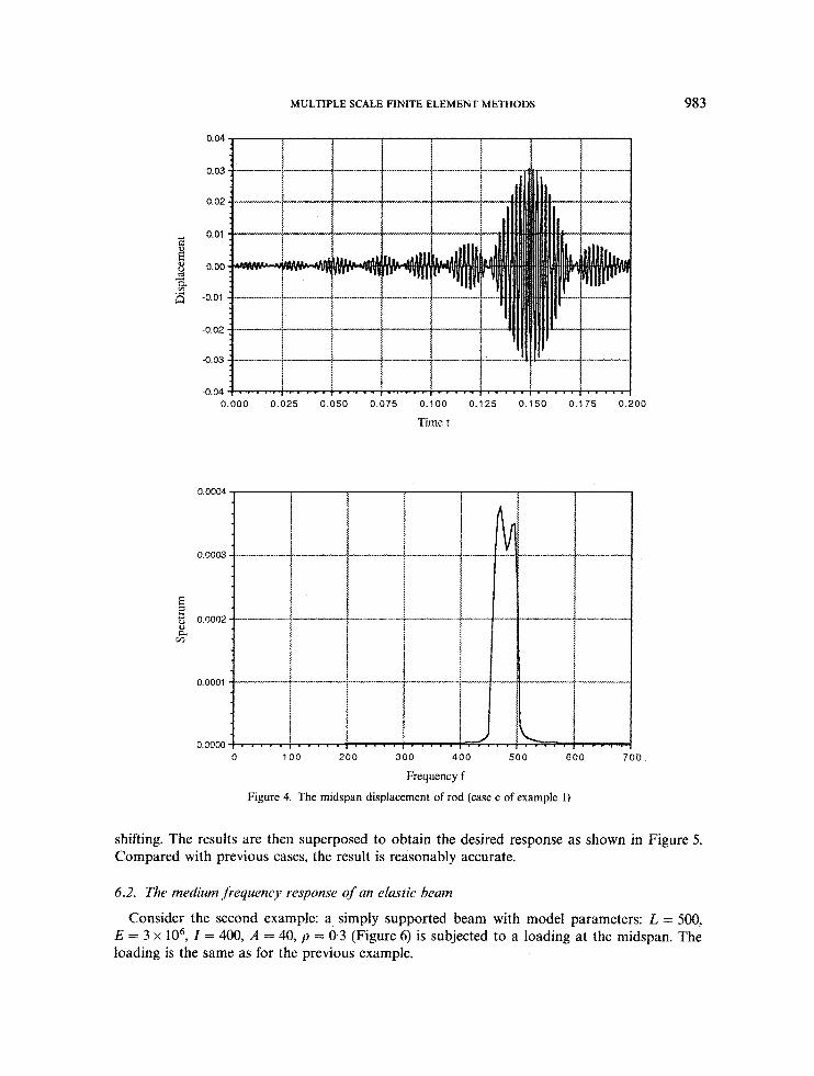
Table I). Figure 4 depicts the midspan displacement in the time and frequency domains. As noted, the result is sufficiently accurate in comparison with case b (see Figure 3).

In order to examine the effect of superposition of band solutions, the band of interest is divided into two bands, namely B19.5 = [2850,3000] and B,,., = [3000,3150]. Using the finite-spectral element for spatial discretization, each band is solved separately by numerical integration with


00

Time t

100 200 300 400 500 600 7 0 0

Frequency f

Figure 4. The midspan displacement of rod (case c of example 1)

shifting. The results are then superposed to obtain the desired response as shown in Figure 5. Compared with previous cases, the result is reasonably accurate.

6.2. The medium frequency response of an elastic beam

Consider the second example: a simply supported beam with model parameters: L = 500, E = 3 x lo6, I = 400, A = 40, p = 0.3 (Figure 6) is subjected to a loading at the midspan. The loading is the same as for the previous example.

0 04

0 03

0 02

0 01

0 00

-0 01

-0 02

-0 03

-0 04 0 0 0 0 0 0 2 5 0 0 5 0 0 0 7 5 0 100 0 125 0 150 0 175 0 2 0 0

Time t

0 100 200 300 400 5 0 0 6 0 0 700

Frequency f Figure 5. The midspan displacement of rod (case d of example 1)

L = 500.0 E = 3,000,000.0 I = 400.0

A = 40.0 r = 0.3

Figure 6. The simply supported beam of example 2

0.000 0.025 0.050 0.075 0.100 0.125 0.150 0.175 0.200

Time t

0 100 200 300 400 500 6 0 0 7 0 0

Frequency f

Figure 7. The midspan displacement of beam (case b of example 2)

Table 11. Summary of results for the beam example

Case a b C d

Frequency band B, r = SO r = 10 r = SO r = 195 and 205 (see equation (1)) Aw = 300 rad/s Aw = 300 rad/s Aw = 300 rad/s Aw = 150 rad/s

Spatial FEM Finite-spectral Wave element Finite-spectral

Time integration unshifted unshifted shifted shifted Time step [ratio] 0~0001 p.01 0.0001 c1.01 0.002 [20] 0.004 [40] No. of time steps 2000 2000 100 50 No. of elements 300 30 60 30 No. of spectral fnc. 6 6 No. of equations 600 240 240 240

discretization


0 000 0 025 0 050 0 075 0 100 0 125 0 150 0 175 0 200

Time t

0 100 2 0 0 300 400 5 0 0 6 0 0 700

Frequency f

Figure 8. The midspan displacement of beam (case c of example 2)

The finite-spectral-element method is used in cases b and d (see Table 11); the wave element method is used in case c. In comparison with case a (the standard finite element method), the total number of equations is reduced significantly. In case c, the response is obtained by integration with shifting, and thus, the time step is relaxed. Case d is similar to the previous example of the rod. Two bands are solved separately and the results are superposed. Comparing results obtained

MULTIPLE SCALE FINITE ELEMENT METHODS

0.000 0.025 0.050 0.075 0.100 0.125 0.150 0.175 0.200

Time t

0 100 2 0 0 ) 400 5 0 0 600

987

10

Frequency f

Figure 9. The midspan displacement of beam (case d of example 2)

in cases b and c (see Figures 6, 7 and 8), the accuracy of the band solution is found to be satisfactory. Results for case d are presented in Figure 9.

7. CONCLUSIONS

In temporal discretization, the method combines techniques of sampling analysis with direct time integration and demonstrates some significant advantages with regard to reduction in the


number of time steps necessary for a simulation. The implementation of such a method presents new features. The solution of each frequency component is independent, so it is well suited for parallel computing. The spectral approaches yield a significant reduction in the number of elements necessary for a simulation while the frequency shifting yields a reduction in the number of time steps required in a simulation.

Future research directions to address are: the choice of bands, since they can be quite important in the resulting accuracy of the response; and the issue of frequency content effect in setting the time step. This may prove to be a rational way of selecting the time step to ensure reasonable accuracy.

APPENDIX I

Clzebysheu polynomials

Chebyshev polynomials denoted by T,( 0, such that 5 E [ - 1.0,1*0], are defined as

T,(cos 6) = cos(n6)

thus

G(5) = 1

T, (5 ) = 5 r,(t) = 252 - 1

G(5) = 4t3 - 35 G(5) = 8t4 - 852 + 1 T,(O = 1655 - 2053 + 55 &(l) = 32t6 - 48t4 + 185' - 1 q(5) = 64t7 - 1125' + 56t3 - 75 &(<) = 1285' - 256c6 + 160t4 - 325' + 1 &(<) = 256c9 - 57617 + 4325' - 120t3 + 95

K O ( ( ) = 512t10 - 12805' + 1120t6 - 400t4 + 505' - 1

T , 1 ( 5 ) = 1024<l1 - 2816t9 + 2816t7 - 12325' + 220r3 - 115 T , 2 ( 5 ) = 20485l' - 61445" + 69125' - 3584t6 + 840t4 - 725' + 1

or

APPENDIX I1

MULTIPLE SCALE FINITE ELEMENT METHODS

where

989

For the case of p = 2:

N 3 ( t ) = 252 - 2

N4(5) = 4t3 - 45 N5(5) = 8 t 4 - 8t2

N6(5) = 16t5 - 20t3 + 45

N7(5) = 3216 - 48t4 + 18t2 - 2

Ns( t ) = 64t7 - 112t5 + 56t3 - 8 t

N9(5) = 1285' - 25616 + 160t4 - 32t2

N I O ( ~ ) = 256t9 - 576t7 + 432t5 - 120t3 + 8t

Nll(5) = 5125" - 1280t8 + 1120t6 - 400t4 + 50t2 - 2

APPENDIX I11

The C1 spectral function

for a = 1,2, . . . Therefore


REFERENCES

1. K. J. Bathe and E. L. Wilson, Numerical Methods in Finite Element Analysis, Prentice-Hall, Englewood Cliffs, N.J.,

2. T. Belytschko and R. Mullen, ‘Stability of explicit-implicit mesh partitions in time integration’, Int. j . numer. methods

3. T. Belytschko, B. Engelmann and W. K. Liu, ‘A review of recent developments in time integration’, State-of-the-Art

4. T. Belytschko, J. Fish and A. Bayliss, ‘The spectral patch-superposition for finite element with high gradients’, Comp.

5. C. M . Bender and S . A. Orszag, Advanced Mathematical Methods for Scientists and Engineers, McGraw-Hill, New

6. E. 0, Brigham, The Fast Fourier Transform, Prentice-Hall, Englewood Cliffs, N.J., 1974. 7. G. M. Fix, ‘Hybrid finite element methods’, SIAM Rev., 18, 460-484 (19%). 8. D. Gottlieb and S . A. Orszag, Numerical Analysis of Spectral Methods: Theory and Applicatons, SIAM, New York,

9. T. J. R. Hughes, The Finite Element Method, Prentice-Hall, Englewood Cliffs, N.J., 1987.

1976.

eng., 12, 1575-1586 (1979).

Surveys on Computational Mechanics, ASME, New York, 1989, pp, 185-199.

Methods Appl. Mech. Eng., to appear.

York, 1978.

1977.

10. T. J. R. Hughes and W. K. Liu, ‘Implicit-explicit finite elements in transient analysis: Stability theory’, J . Appl. Mech.,

11 . T. J. R. Hughes and W. K. Liu, ‘Implicit-explicit finite elements in transient analysis: Implementation and numerical

12. T. Igusa and A. Der Kiureghian, ‘Dynamic response of multiply supported secondary systems’, J . Eng. Mech. ASCE,

13. W. K. Liu, ‘Development of mixed time partition procedures for thermal analysis of structures’, Int. j . numer. methods

14. W. K. Liu and Y. F. Zhang, ‘Unconditionally stable implicit-explicit algorithms for coupled thermal stress waves’,

15. W. K. Liu, T. Belytschko and K. C. Park, Innovative Methods for Nonlinear Problems, Pineridge Press, Swansea, U.K.,

16. W. K. Liu, T. Belytschko and Y. F. Zhang, ‘Implementation and accuracy of mixed-time implicit-explicit methods for

17. W. K. Liu, T. Belytschko and Y. F. Zhang, ‘Partitioned rational Runge Kutta for parabolic systems’, Int. j . nullper.

18. A. H. Nayfeh, Perturbation Methods, Wiley Interscience, New York, 1969. 19. A. T. Patera, ‘Spectral element method for fluid dynamics: Laminar flow in channel expansion’, J . Comp. Phys., 54,

20. M. R. Ramirez and T. Belytschko, ‘An expert system for setting timesteps for dynamic finite element programs’, Eng.

21. J. L. Sackman and J. M. Kelly, ‘Seismic analysis of internal equipment and components in structures’, Eng. Struct., I,

22. C. Soize, ‘Medium frequency linear vibrations of anisotropic elastic structures’, Rech. Aerosp., 1983. 23. C. Soize and D. R. Ohayon, Private communication, ONERA, France, 1987. 24. G. Strang and G. J. Fix, An Analysis of the Finite Element Method, Prentice-Hall, Englewood Cliffs, N.J., 1973. 25. Y. Zhang and R. S. Harichandran, ‘Eigenproperties of classically damped MDOF composite system’, J . Eng. Mech.

26. Y. Zhang and R. S. Harichandran, ‘Implicit subdomain integration for dynamic analysis of large-scale structural

45, 371-374 (1978).

examples’, J . Appl. Mech., 45, 375-378 (1978).

111, 20-40 (1985).

eng., 19, 125-140 (1983).

Comp. Struct., 17, 371-374 (1983).

1984.

structural dynamics’, Comp. Struct., 19, 521-530 (1984).

methods eng., 20, 1581-1597 (1984).

468-488 (1984).

Comp., 5, 205-219 (1989).

179-190 (1979).

ASCE, 115, 1515-1526 (1989).

systems’, Comp. Methods Appl. Mech. Eng., to appear.

Multiple scale finite element methods

Documents

Transcript of Multiple scale finite element methods