finite element models and experimental validation - POLITesi

POLITECNICO DI MILANO

School of Industrial and Information Engineering

Master Degree in

Mechanical Engineering

Study of tyre-rim interaction:

finite element models and experimental validation

Relatore: Gianpiero MASTINU

Correlatore: Federico Maria BALLO

Master Degree Thesis

Filippo Galli

Student ID: 835951

Contents

1 Introduction 81.1 Functions and geometry of the alu-

minium alloy rim . . . . . . . . . . . 8

1.2 Standard code for car wheel . . . . 10

1.3 The aluminium alloy rim manufac-turing processes . . . . . . . . . . . . 10

1.4 Aim of this thesis . . . . . . . . . . . 11

1.5 Outline . . . . . . . . . . . . . . . . . 12

2 Actual techniques of car rim design - Stateof the art 142.1 Static case . . . . . . . . . . . . . . . 14

2.2 Optimization of the rim shape . . . 20

2.3 Fatigue analysis . . . . . . . . . . . . 22

3 Experimental campaign 283.1 Aim of the experiment . . . . . . . . 28

3.2 Structure of the campaign . . . . . . 28

3.3 Description of the tested wheel . . . 29

3.4 The experimental bench . . . . . . . 30

3.5 Description of used instruments . . 34

3.6 Evaluation of the radial sti�ness ofthe wheel . . . . . . . . . . . . . . . . 40

3.7 Evaluation of the lateral sti�ness ofthe wheel . . . . . . . . . . . . . . . . 41

3.8 E�ect of the in�ation pressure onthe stress/strain state of the rim . . 42

1

3.9 E�ect of radial and lateral load onthe stress/strain state of the rim . . 44

3.10 Summary of experimental campaign 52

4 FE models 534.1 Complete Model . . . . . . . . . . . 54

4.1.1 Rim . . . . . . . . . . . . . . 54

4.1.2 Tire . . . . . . . . . . . . . . 56

4.1.3 Assembly, Interactions andConstraints . . . . . . . . . . 59

4.1.4 Load steps . . . . . . . . . . . 62

4.1.5 Simulated loadcases . . . . . 63

4.2 Intermediate model . . . . . . . . . . 64

4.2.1 Parts . . . . . . . . . . . . . . 64

4.2.2 Load steps . . . . . . . . . . . 64


4.3 Simpli�ed model . . . . . . . . . . . 69

4.3.1 Part and material . . . . . . 69

4.3.2 Boundary conditions and loads 69


5 Analysis of results and comparison amongmodels 785.1 Validation of assigned material prop-

erties . . . . . . . . . . . . . . . . . . 78

5.2 Analysis of the stress/strain �eld onthe wheel . . . . . . . . . . . . . . . . 82

5.3 Comparison between models . . . . 89

6 Conclusions 91

2

List of Figures

1 Aluminium alloy rim parts and parameters . . . . . . . . . . . . 82 Di�erent o�ets . . . . . . . . . . . . . . . . . . . . . . . . . . . . 93 PCD illustration . . . . . . . . . . . . . . . . . . . . . . . . . . . 94 Example of a code on an aluminium alloy car rim . . . . . . . . . 105 Scheme of a cast mold for an aluminium alloy rim . . . . . . . . 116 The reference directions . . . . . . . . . . . . . . . . . . . . . . . 147 A schematic showing the load induced by tire inner pressure. . . 158 Cosine loading function . . . . . . . . . . . . . . . . . . . . . . . 169 Boussinesq loading function . . . . . . . . . . . . . . . . . . . . . 1610 Eye-bar loading function . . . . . . . . . . . . . . . . . . . . . . 1711 Tire analytical model with a distributed load and free-body dia-

gram of a portion ds of the curved beam [6] . . . . . . . . . . . . 1812 Tyre model used in [6] and node sets for load application . . . . 1913 Distributed nodal reaction forces acting on the rim in radial (left)

and axial (right) directions: 200/70 R17 rear tire, in�ation pres-sure 1.8 bar, and vertical load 2950 N. [6] . . . . . . . . . . . . . 19

14 Rim FE model subdivided in 2 domains . . . . . . . . . . . . . . 2015 Results of optimization . . . . . . . . . . . . . . . . . . . . . . . . 2116 Loads application for �nal veri�cation . . . . . . . . . . . . . . . 2117 Layout of wheel rotary fatigue test . . . . . . . . . . . . . . . . . 2318 Radial fatigue test machine . . . . . . . . . . . . . . . . . . . . . 2319 The biaxial fatigue load test machine . . . . . . . . . . . . . . . . 2420 Example of a real biaxial test . . . . . . . . . . . . . . . . . . . . 2421 3D model of the biaxial wheel test system: (a) whole model; (b)

cut view of the model. . . . . . . . . . . . . . . . . . . . . . . . . 2522 FEM of the biaxial wheel test system (for strength analysis). . . 2623 Global view of the experimental bench . . . . . . . . . . . . . . . 2824 The rim used for the experiment . . . . . . . . . . . . . . . . . . 2925 Dimensions of used tire . . . . . . . . . . . . . . . . . . . . . . . 3026 Calibration turret . . . . . . . . . . . . . . . . . . . . . . . . . . . 3127 Vertical guide . . . . . . . . . . . . . . . . . . . . . . . . . . . . . 3128 Assembly showing plates, guides and rollers. . . . . . . . . . . . . 3229 Calibration turret, where all components are visible . . . . . . . 3230 Wheel support . . . . . . . . . . . . . . . . . . . . . . . . . . . . 3331 Adaptation �ange . . . . . . . . . . . . . . . . . . . . . . . . . . . 3332 S.G. properties from HBM catalogue . . . . . . . . . . . . . . . . 3433 S.G. rosette properties from HBM catalogue . . . . . . . . . . . . 3534 Strain gauges positions . . . . . . . . . . . . . . . . . . . . . . . . 3635 Half-bridge layout . . . . . . . . . . . . . . . . . . . . . . . . . . 3636 Compensation plate . . . . . . . . . . . . . . . . . . . . . . . . . 3737 6-axis load cell . . . . . . . . . . . . . . . . . . . . . . . . . . . . 3938 Lateral �Celesco� . . . . . . . . . . . . . . . . . . . . . . . . . . . 3939 Di�erent loading curves with the evaluated sti�nesses . . . . . . 41

3

40 Lateral displacement- Lateral force curve, in�ation pressure 4.5bar, Loadcase 1 . . . . . . . . . . . . . . . . . . . . . . . . . . . . 41

41 Measurements in the di�erent channels under the e�ect of in�at-ing pressure . . . . . . . . . . . . . . . . . . . . . . . . . . . . . . 42

42 Biaxial test, Pressure 4.5 bar, Orientation 0° . . . . . . . . . . . . 4643 Biaxial test, Pressure 4.5 bar, Orientation 36° . . . . . . . . . . . 4744 Vertical load time history, In�ation pressure 2.5 bar, Orientation

0° . . . . . . . . . . . . . . . . . . . . . . . . . . . . . . . . . . . . 5145 Model of the rim . . . . . . . . . . . . . . . . . . . . . . . . . . . 5446 Particulars of half-rim where the strain gauges partitions are visible 5547 Picture of the meshed assembly . . . . . . . . . . . . . . . . . . . 5548 C3D10 tet. element . . . . . . . . . . . . . . . . . . . . . . . . . . 5649 Particular of the rim with a thiker mesh in the S.G. areas . . . . 5650 Tire pro�le . . . . . . . . . . . . . . . . . . . . . . . . . . . . . . 5751 FE model cross section where all parts are highlighted . . . . . . 5852 C3D8 hex. element . . . . . . . . . . . . . . . . . . . . . . . . . . 5953 Half-section of the meshed tire . . . . . . . . . . . . . . . . . . . 5954 Assembly . . . . . . . . . . . . . . . . . . . . . . . . . . . . . . . 6055 Contact surfaces . . . . . . . . . . . . . . . . . . . . . . . . . . . 6156 Assembly picture, where RP and constrains are highlighted . . . 6157 In�ating pressure application . . . . . . . . . . . . . . . . . . . . 6258 Tire 2-D model, where in�ation pressure and maximum displace-

ment constraint are applied . . . . . . . . . . . . . . . . . . . . . 6559 Tire 3-D model, with the encastre boundary conditions highlighted. 6560 Tire-rim interaction surface where the encastre is loacated . . . . 6661 Example of a path where resultant lateral and radial forces are

computed . . . . . . . . . . . . . . . . . . . . . . . . . . . . . . . 6662 Reaction forces per unit length at the tire-rim interface . . . . . 6763 Nodes for the application of the resultant reactions forces on the

tire beads. . . . . . . . . . . . . . . . . . . . . . . . . . . . . . . 6864 View of the rim model, whose material has been assigned . . . . 6965 View of the constrained rim . . . . . . . . . . . . . . . . . . . . . 7066 Dimensions involved in in�ation pressure load . . . . . . . . . . . 7167 Pressure lateral load on the rim �ange. . . . . . . . . . . . . . . . 7168 Surface where in�ating pressure acts directly . . . . . . . . . . . 7269 Lateral schematic view of the wheel, useful to calculate the load-

ing arc . . . . . . . . . . . . . . . . . . . . . . . . . . . . . . . . . 7370 View of the rim where the arc ±50°is highlighted on the bead

seat and on the �ange . . . . . . . . . . . . . . . . . . . . . . . . 7471 Radial load applied on the inner and outer beas seats . . . . . . 7572 View where the C-SYS used in the Analytical �eld is highlighted 7673 Lateral loads acting on the inner and outer �anges . . . . . . . . 7674 Example of a radial displacement of the tire-plate contact point

in the 'Complete Model' . . . . . . . . . . . . . . . . . . . . . . . 7875 Example of vertical reaction force . . . . . . . . . . . . . . . . . . 7976 Loading curves in the di�erent cases . . . . . . . . . . . . . . . . 79

4

77 Simulated and experimental lateral loading curves, 'Loadcase 1',pressure 4.5 bar . . . . . . . . . . . . . . . . . . . . . . . . . . . . 80

78 Particular of the wheel deformation under lateral load, �CompleteModel� . . . . . . . . . . . . . . . . . . . . . . . . . . . . . . . . . 81

79 Local C-SYS . . . . . . . . . . . . . . . . . . . . . . . . . . . . . 8280 Strain E11 on a strain gauge base . . . . . . . . . . . . . . . . . . 8381 Deformed shape and displacements due to radial load . . . . . . 88

5

List of Tables

1 Ki evaluated for each strain gauge . . . . . . . . . . . . . . . . . 382 Technical data of the 6-axis load cell . . . . . . . . . . . . . . . . 383 Loading points and radial sti�nesses . . . . . . . . . . . . . . . . 404 Strain induced by 4.5 bar in�ating pressure . . . . . . . . . . . . 435 Read strains for the analyzed loadcases, orientation 0° . . . . . . 456 Read strains for the analyzed loadcases, orientation 36° . . . . . 477 Read strains for the analysed loadcases, orientation 72° . . . . . . 488 Read strains for the analyzed loadcases, orientation 108° . . . . . 499 Read strains for the analyzed loadcases, orientation 144° . . . . . 4910 Read strains for the analyzed loadcases, orientation 180° . . . . . 5011 Read strains for the analyzed loadcases, in�ation pressure 2.5 bar,

orientation 0° . . . . . . . . . . . . . . . . . . . . . . . . . . . . . 5012 Material properties of the tire structure ( from [21, 22]) . . . . . 5813 Geometric properties of reinforcements (from [21, 22]). . . . . . . 5814 Radial sti�ness of the wheel . . . . . . . . . . . . . . . . . . . . . 8015 Lateral sti�ness of the wheel . . . . . . . . . . . . . . . . . . . . . 8016 Vertical loadcase, Pressure 4.5 bar, orientation 0° . . . . . . . . . 8417 Loadcase 1, Pressure 4.5 bar, orientation 0° . . . . . . . . . . . . 8418 Loadcase 3, Pressure 4.5 bar, Orientation 0° . . . . . . . . . . . . 8519 Loadcase 1, Pressure 4.5 bar, Orientation 36° . . . . . . . . . . . 8520 Loadcase 3, Pressure 4.5 bar, Orientation 36° . . . . . . . . . . . 8621 Vertical Loadcase, Pressure 2.5 bar, Orientation 0° . . . . . . . . 8622 E�ect of in�ation pressure, using �Simpli�ed Model� . . . . . . . 87

6

Abstract

This thesis deals with the design of aluminium alloy car wheel. It is focused onhow di�erent loads are transferred from the tire to the rim. In particular, thecase of biaxial load (i.e. radial and lateral) is analyzed. Three di�erent FiniteElements models have been developed. They are charachterized by di�erentlevels of complexity: the simplest model, consists only in the rim. The loadsare directly applied on a loading arc, whose extension depends on the actualdeformation of the tire under the loads. Vertical and lateral loads are applied bymeans of a cosine function. It is also the most interesting one, because the anal-ysis is very fast and a few input parameters are required. The second presentedmodel is more detailed and involves both the rim and the tire. The reactionson the tire-rim interface are obtained by applying the radial and lateral loadsand the in�ation pressure to the tire. Then, they are moved to the bead seatsto evaluate the stress/strain �eld of the wheel. The most complete developedmodel is made up of the rim, coupled with the in�ated tire in a single assem-bly. The loads are provided through the contact with a rigid plane, simulatingthe real condition of a car running on an asphalt road. A lot of information isrequired to carry out a simulation using these last two models. A very powerfulcomputer is needed, as well.

The accuracy of the developed models is discussed and validated by com-paring the strain �eld of the rim with measured experimental values. For thispurpose, an experimental bench is built for reproducing exactly the load condi-tions simulated through FEA. The strains on the surface of the component aremeasured thanks to some strain gauges placed both on the spokes and on therim channel. These values are, then, compared with the simulated ones in thesame positions.

At last, possible applications are suggested for each model, especially for thesimplest one, being su�ciently reliable, fast and easy to set at the same time.

Keywords: wheel, rim, tire, ABAQUS, tire-rim interface, stress/strain �eld.

7

1 Introduction

1.1 Functions and geometry of the aluminium alloy rim

The aluminium alloy car rim has various technical functions. It connects thecar hub with the tire, and it must keep also the in�ation pressure, since tubelesstire are nowadays widespread. Being in such a position, it has to withstanda great number of loads, as the car own weight, the loads generated while itis rolling, while a traction/braking torque is impressed, or a bending torquethat is generated while the car is running into a curve. In addition to these, itshould provide also a proper aeration to the components of the hub (for examplebrakes) to avoid their overheating. The design of the component must take intoaccount all these aspects and is, therefore, a very hard and expensive task. Thealuminium rim, thanks to the material properties, allows to achieve a betterweight/resistance ratio then the steel one and it is, for this fact object of agreat number of studies and researches, like this one. Before starting with thethesis it is important to keep in mind the di�erent parts that make the rim upand their names; they will be mentioned lots of times. There are also di�erentparameters which a�ect the design, like the rim channe width, the O�set or ET,and the PCD, that is a�ected by the number, the diameter and the distance ofthe �xing holes. Fig.1.

Figure 1: Aluminium alloy rim parts and parameters

The rim channel

The channel is the portion of the rim where the tire is �xed 1. Its pro�lesare de�ned by the standard ETRTO (European Tires and Rims Technical Or-ganization): H (Hump), FH (Flat Hump), EH2 (Extemdemd Hump), EH2+(Extended Hump for Flat Tires). The tire width depends, of course, on the therim pro�le one, whose dimensions, for every di�erent rim diameters, are de�nedby ETRTO, as well. Wrong dimensions may lead to poor adhesion between thetire and the rim, or a problem in in�ation phase or in maintaining a stable airpressure.

8

The o�set (ET)

The o�set is the distance, in millimeters, between the contact surface betweenthe hub and the rim, and the axis of the rim itself. It can be positive, nullor negative (Fig.2). Having the same rim width, the wheel can be protudedoutward or inward by changing the o�set. However, a too low ET can lead to ahigh wear of bearings and suspension parts, or it can even negatively a�ect thecar handling.

Figure 2: Di�erent o�ets

The PCD

PCD (Pitch Circle Diameter) refers to the number, position and distance of therim �xing holes. Every aluminium alloy rim is characterized by a number ofholes, whose centers are located at a certain distance from the center of thewhole rim.. It is a very important parameter, as it allows the rim componentto �x properly to the hub.

Figure 3: PCD illustration

9

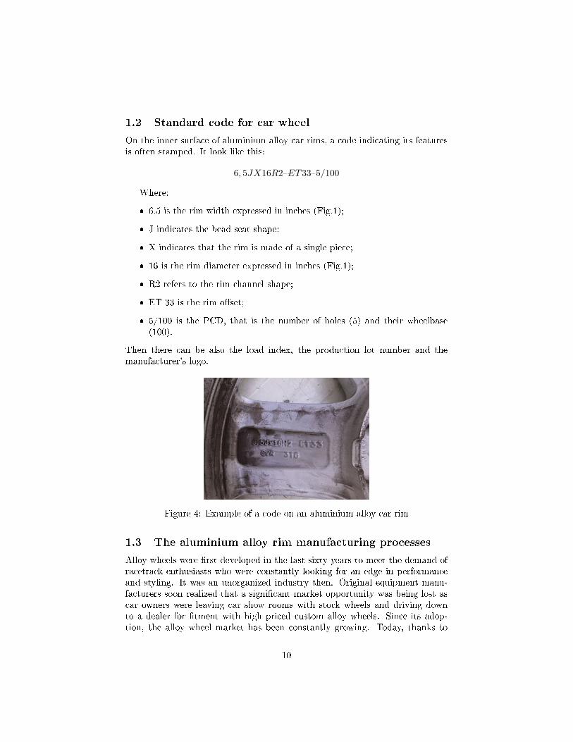
1.2 Standard code for car wheel

On the inner surface of aluminium alloy car rims, a code indicating its featuresis often stamped. It look like this:

6, 5JX16R2�ET33�5/100

Where:

� 6,5 is the rim width expressed in inches (Fig.1);

� J indicates the bead seat shape;

� X indicates that the rim is made of a single piece;

� 16 is the rim diameter expressed in inches (Fig.1);

� R2 refers to the rim channel shape;

� ET 33 is the rim o�set;

� 5/100 is the PCD, that is the number of holes (5) and their wheelbase(100).

Then there can be also the load index, the production lot number and themanufacturer's logo.

Figure 4: Example of a code on an aluminium alloy car rim

1.3 The aluminium alloy rim manufacturing processes

Alloy wheels were �rst developed in the last sixty years to meet the demand ofracetrack enthusiasts who were constantly looking for an edge in performanceand styling. It was an unorganized industry then. Original equipment manu-facturers soon realized that a signi�cant market opportunity was being lost ascar owners were leaving car show rooms with stock wheels and driving downto a dealer for �tment with high priced custom alloy wheels. Since its adop-tion, the alloy wheel market has been constantly growing. Today, thanks to

10

a more sophisticated and environmentally conscious consumer, the use of alloywheels has become increasingly relevant. With this increased demand came newdevelopments in design, technology and manufacturing processes to produce asuperior with a wide variety of designs. The key to an have a good alloy wheelis the quality of the casting. The casting integrity depends on the process used.Wheels have been made using various casting techniques such as sand casting;gravity die casting, centrifugal, squeeze and low pressure die casting. Sand andgravity castings are less controllable operations and have problem with blowholes and shrinkages. Hence these wheels are generally not preferred by inter-national OEMs. Centrifugal and squeeze casting yields a good quality wheel, buthave the disadvantage of being unable to manufacture non-axis metric designwheels. Such a technology has not become popular. Low pressure die casting(Fig.5) allows precise control during the casting and cooling cycle. Signi�cantlyreducing cavities, porosity and uneven shrinkage. This technology is amenableto large scale production and automation, and is today considered as the stateof the art technology for manufacture of alloy wheels. Low pressure die castingare incorporated by most of the world's leading rims suppliers.

Figure 5: Scheme of a cast mold for an aluminium alloy rim

1.4 Aim of this thesis

Automotive wheels have complicated geometry and they must satisfy manifolddesign criteria, such as style, weight, manufacturability, and performance. Inaddition to a fascinating wheel style, wheel design also needs to accomplish a lotof engineering objectives including some necessary performance and durabilityrequirements (sub.1.1). Moreover, in order to ensure driving performances andgood road handling characteristics, the wheel must be as light as possible [2, 7].Nowadays, reduction in wheel weight is a major concern in wheel industry1. Forwheel manufacturers, reduction in wheel weight means a reduction in material

1All the great advantages of a car lightweight design can be found in [2]

11

cost. In order to reduce the manufacturing cost, wheel weight must be min-imized, while wheel must still have enough mechanical performance to su�ernormal or severe driving conditions. Traditionally, wheel design and develop-ment is very time consuming, because it needs a number of tests and designiterations before going into production. In modern industry, how to shorten de-velopment time and to reduce the number of times of test are important issues.In order to achieve the above objectives, computer aided engineering (CAE) isa useful tool and it has been recently introduced in the wheel design.

This study is, therefore, aimed to develop and compare di�erent FE modelsto better simulate the transmission of loads from the tire to the rim during thedesign of the component. It is a critical point, as, generally, the resultant forcesthe wheel has to endure are known, but how they are transmitted and distributedat the tire/rim interface is very di�cult to understand, because of the in�uenceof the in�ation pressure and of the geometry of the tire. In fact the tire is avery complex system, made of di�erent materials, sometimes with highly non-linear behaviour, and it is coupled to the rim thanks to the beads. Therefore, adeep knowledge of this aspect is absolutely necessary to provide a more reliableanalysis of the state of stress/strain of the rim, allowing an optimized design ableto accomplish the more and more demanding requests in term of performance,lightweight, reliability and optimal design of the market, perhaps reducing costsand time, which, for di�erent reasons, may be unsustainable.

1.5 Outline

Chapter 2 is dedicated to the literature review and to the actual methodsadopted to analyze the resistance properties of the component. It is subdividedin three subsections: the �rst one shows how to deal with the di�erent types ofstatic loads, which the wheel can be subjected to, in a FE analysis, according towhat has been studied so far. Therefore, di�erent methods for the application ofthe loads due to the car's own weight and to the in�ating pressure are presented.In second one a shape optimization problem is brie�y described, highlightingthe reason why a study of a more realistic way to apply the loads may lead tobetter results. The third subsection is dedicated to the dynamic analysis: theactual standard tests (cornering fatigue test, radial test and biaxial test) aredescribed together with the actual attempts to simulate them through a FEsoftware. As in the previous cases, both the positive and negative sides of theactual procedures for testing the component are presented, showing how thisresearch can achieve better results in an easier way.

In Chapter 3 the experiment that is set to investigate how radial and lat-eral loads a�ects the stress/strain �eld of the rim is carefully described. At �rstthe components used and all the equipment are presented. Some pages are ded-icated to the calibration of the instruments, like the strain gauges, and to thepreparation of the experimental bench. At last all the needed data are collectedand processed: the in�uence of in�ation pressure, of radial and lateral load onthe stress/strain �eld of the rim are investigated by collecting the values coming

12

from the di�erent strain gauges in di�erent loadcases. The radial sti�ness of thewheel is then calculated for di�erent in�ation pressures. All these data will beused to develop and validate the three FE model presented later.

In Chapter 4 all the developed FE models, featured by di�erent level of com-plexity, are presented,. The �rst one is a very detailed model because boththe tire and the rim are reproduced and put together in a very heavy assem-bly. A lot of parameters are needed, above all the tire structure and materialproperties must be known. This may represent a limit since the knowledge ofthem is, sometimes, di�cult, expensive and time consuming. In addition tothis its computational time is very long and a powerful hardware is compul-sory. Then, another model is described, where stresses/strains in the rim areanalyzed separately. This reduces the computational time, but require a morecareful evaluation of the nodal reaction forces in the tire/rim interaction area.Being the tire present in the model, all the parameters involved must be known,as well. Therefore, a simpler FE model, consisting in the only rim with theloads directly applied on it, is developed and described in details. The analysisin this case is much faster, easier and cheaper; for these reasons the attentiondedicated to its setting is high.

Chapter 5 is dedicated to the presentation, processing and discussion of thedi�erent outputs of the simulations. At �rst the procedure adopted to set themodels, check the reliability and the verify the consistency of the various param-eters involved is described. Then, after the simulations have been performed,the strains in the gauges spots are collected, listed and compared to the ex-perimental values to check the validity of the models. Di�erent loadcases areobserved and the in�uence of each di�erent load is analyzed by looking at theobtained values. The very last part of the chapter is about the comparisonbetween the models, the advantages or disadvantages of each one with respectto the others are described there.

The �nal Chapter 6 contains the summary of the whole study and of theresults obtained; it aims to better focus the reader's attention on the innovationand bene�ts that such an analysis has introduced in the design of the car rims.At last a few pages are spent to describe possible applications and improvementsof the presented models.

13

2 Actual techniques of car rim design - State ofthe art

2.1 Static case

To understand how the loads are tranferred from the ground to the rim, passingthrough the tire, the study of the static case (i.e. where the car is not moving),plays a central role. Such a situation will be carefully described and simulatedin this thesis, but di�ent examples of similar analysis are already present in thescienti�c environment. [1, 3]

Figure 6: The reference directions

At �rst it is necessary to de�ne what loads are acting when the wheel isstatically standing the weight of the car: basically the in�ating pressure of thetire and the weight of the car itself2 are acting. Now let's have a look on howthey have been simulated by scienti�c community so far:

In�ation pressure

It is the inner tire pressure that withstands the weight of the car, but it also pro-vide the required load to mantain itself inside the room between the rim channeland the tire, by pushing the beads into their seats and against the �anges. Thisgenerates an additional load on the rim that can not be neglected. Accordingto [1], air pressure is a constant load having little to no relation to rotation ofthe automobile wheel unit. In a three-dimensional analysis, the stress-inducedon the non-axisymmetrically shaped disc is assumed to be negligible. Conse-quently, an axisymmetric analysis is adequate for purposes of calculating theinduced stress under the in�uence of tire air pressure. The in�ation pressureacts directly on the outer side of the aluminium alloy rim and indirectly on its�ange, by pushing the beads.

2As matter of fact, it can be assumed that the weight of the car is divided on front andrear axis following a certain ratio given by the manufacturer and equally distributed on rightand left wheel

14

Figure 7: A schematic showing the load induced by tire inner pressure.

The air pressure, pressing on the sidewalls of the tire, generates the lateralload, which acts in an axial direction. This load varies according to the type oftire, its aspect ratio of the cross section , and its reinforcements [4]. Consideringthe pro�le of the cross section of the tire and rim assembly, shown in A schematicshowing the load induced by tire inner pressure., the axial component of theforce (Wp), which results from an in�ation of the tire (P0) is calculated usingthe relations:

Wp = π(a2=r2f )P0 [N ] (1)

Where a is the design radius of the tire and rf is the radius at the loadingpoint on the rim �ange. Since the axial load is supported by the tread of thetire and the rim �ange, approximately a half of the load is assumed to be loadedonto each part[1]. Thus, the load on a unit circumferential length of the rim�ange (Tf ) is expressed as:

Tf =Wp

2Ö2ÖπÖrf= (a2 − r2f )

P0

4Örf[N/m] (2)

Radial load

After having applied a vertical load to the wheel, the tire undergoes a deforma-tion depending on its radial sti�ness. The bead is, therefore, pressed againstthe bead-seat. To evaluate the magnitude and the distribution of this pressureis rather complex, but in the scienti�c licterature there are di�erent solutions:

� Cosine loading function (CLF)[1] suggests to apply a cosine function on the bead seats that looks like:

Wr = W0cos

(π

2

ϕ

ϕ0

)[N/m2] (3)

Where ϕ0 depends on the tire deformation and so on its radial sti�ness,but a value of 40° is suggested for common applications. By integrating

15

that function along the whole arc a analytical expression to W0 comes:

W0 =Wπ

4brbϕ0[N/m2] (4)

Where rbis the radius of the bead and b is the width of the bead seat.

Figure 8: Cosine loading function

� Boussinesq loading function (BLF)This solution[3] reproduces the tensions and deformations generated by aforce orthogonally applied to a surface in an ideal, continuous, homoge-neous, isotropic, linear elastic and weightless semi-space. The analyticalsolution, which can be implemented in a numerical model, looks like:

ϕ(r, ϑ) = =K

2rsinϑ (5)

By integrating the function along the pro�le, the constantK can be found:

K =P

π(6)

Where P is the vertical load acting on the wheel.

Figure 9: Boussinesq loading function

16

� Eye-bar loading function (ELF)This model considers the pressure distribution usually exchanged betweena round shaped rod and a hub, without any interspace. The load per unitlength distribution on the beads is:

W = 2r

π/2ˆ

0

qcosϑdϑ [N ] (7)

The maximum stress (i.e. for ϑ = 0) is:

qmax =2W

πr[N/m] (8)

Figure 10: Eye-bar loading function

Other analytical and numerical solutions

More detailed analytical and numerical solutions are presented and carefullydescribed in [6] for motor-bike wheel. The reaction forces acting on the wheel rimwhen a vertical load is applied are explicitly computed. The model is depictedin Fig.11a and consists of an external deformable curved beam connected to thewheel rim by means of linear springs. The linear springs are actually modeled asa distributed spring (sti�ness per unit of length). The wheel rim is assumed as arigid body; therefore, the internal ring is �xed to the ground. The model, whenloaded by a vertical load, is symmetric with respect to a vertical axis passingthrough the center of the tire. The curved beam accounts for the bendingsti�ness of the tread, described by the parameter EJ . k [N/mm2] is the residualradial sti�ness per unit of length of the tire carcass. In the radial sti�ness k, thesti�ening e�ect of the in�ation pressure is also considered. EJ and k representthe physical properties of the tire and, therefore, their numerical values havebeen identi�ed for the actual tire under consideration[6]. After an analysis ofthe equilibrium equations on a portion ds de�ned by an in�nitesimal angle dφof a general curved beam (Fig.11b), an analytical relation, for the most realisticcase considered (i.e. with the vertical load applies as a distributed pressure),

17

follows this relation:

d5u

dφ5+ 2

d3u

dφ3+

(1 +

k(u)r4

EJ+

r4

EJ

dk(u)

duu

)du

dφ+

r4

EJ

dq(φ)

dφ= 0 (9)

It can be solved considering its own boundary conditions which take into accountthe load applied, the symmetry of the wheel, its geometry and so on. In theformula9, u is the radial displacement, k is the tire residual sti�ness, EJ ar thematerial parameter of the radial curved beam simulating the tire section, q isthe load distribution and φ is the considered angle.

(a) Wheel analytical model (b) In�nitesimal portion of beam

Figure 11: Tire analytical model with a distributed load and free-body diagramof a portion ds of the curved beam [6]

On the other hand a numerical model has been developed, using the sameidea of the analytical one. A 3D FE model of tire is generated thanks to thesweep extrusion of the 2D axisymmetric pro�le, previously deformed by itsin�ation pressure. Thus, the 3D model is constrained in the beads with anencastre and both radial and lateral loads are applied to it, by pushing a rigidplate radially and laterally to simulate the contact with the asphalt. The nodalreaction forces are, then, evaluated, summed up along the beads and transferredto the bead seats on the rim surface (Fig.12). The stress/strain �eld of the rimis, under these loads, obtained.

18

Figure 12: Tyre model used in [6] and node sets for load application

In Fig. 13, there are some examples of the the two di�erent solutions com-pared for the same load.

Figure 13: Distributed nodal reaction forces acting on the rim in radial (left)and axial (right) directions: 200/70 R17 rear tire, in�ation pressure 1.8 bar, andvertical load 2950 N. [6]

Later in the report, these ideas will be applied also to a car wheel anddiscussed in detail.

Other studies can be found in the literature about the simulation and predic-tion of the contact forces generated at tyre road interaction (for instance the wellknown book by Pacejka [7]). In few papers, however, the tire rim/interactionis investigated. In many other cases, the load acting on the tire are roughlyestimated by too simple distributions: in [8], for example, the vertical load issimply applied in two reference points, coupled to an arc of the wheel circumfer-ence. No time is dedicated to investigate the width of the arc or the distributionof those forces. As it will be shown later, this approach can lead to an overes-timation of the stresses/strains in some sections of the component if they arelocated in a too narrow arc, or to an unrealistic deformed shape if the arc is toowider. In other cases, like [9], the same load is applied as a non-better-de�ned�pressure at the rim�. Therefore, a dedicated study is needed to look into thisaspect, in order to estimate the stress/strain �eld and the deformed shape ofthe car component in the realistic way possible.

19

2.2 Optimization of the rim shape

To supply to the always increasing requests of lightweight design, one step be-yond can be done by choosing materials with better resistance to mass ra-tios. However, a signi�cant mass reduction (till 50 % of the total mass) can beachieved by giving a clever shape to the wheel. [8] suggests a procedure: the rimis subdivided in 2 domains, the one that should be optimized, which constitutesthe optimization design space, consisting in the hub and in the spokes sectionand the one that should not, that is the rim channel (Fig.14).

Figure 14: Rim FE model subdivided in 2 domains

A topological optimization is, then, implemented by following these steps.

1. De�nition of a CAD model of the solid wheel

2. De�nition of the marerial that will compose the wheel

3. Implementation of the optimization algorithm. At �rst, the radial load isapplied: the resultant forces is simply divided in two di�erent punctualforces and applied in two reference points as in Fig.14. Those points are,then, coupled to an arc of the wheel circumference, located on the beadseats surfaces. An encastre constraints is, then, placed in the hub. Theoptimization procedure is, now, performed, using one of the structuraloptimization algorithms already included in an ABAQUS solver, like HY-PERMESH, aimed to reduce the material used, being, at the same timeable to resist to the applied loads. The useless material is, in this way,removed and the �nal shape is obtained (Fig.15)

20

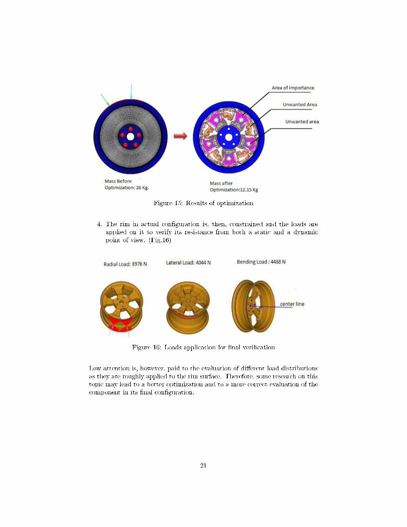
Figure 15: Results of optimization

4. The rim in actual con�guration is, then, constrained and the loads areapplied on it to verify its resistance from both a static and a dynamicpoint of view. (Fig.16)

Figure 16: Loads application for �nal veri�cation

Low attention is, however, paid to the evaluation of di�erent load distributionsas they are roughly applied to the rim surface. Therefore, some research on thistopic may lead to a better optimization and to a more correct evaluation of thecomponent in its �nal con�guration.

21

2.3 Fatigue analysis

The �rst dictionary de�nition of fatigue deals with weariness from labor orexertion for tired material. The appropriate de�nition is the tendency of amaterial to break under repeated cyclic loading at a stress considered lowerthan the tensile strength in a static test. Fatigue cracks can terminate theusefulness of a structure or component by more ways than just fracture. Fatigueresistance must be, therefore, carefully evaluated for all the components andstructures subjected to repeated loading conditions. It is one of the most di�cultdesign issue to solve. Experience has shown that large percentage of structuralfailures are attributed to fatigue and as a result, it is an aspect which has beenand will continue to be the main object of some researches. Related loadingsof a component or structure and stresses that are not dangerous if staticallydistibuted, may cause a crack or racks to form. Under cyclic loading thesecracks may continue to grow and cause a failure, when the remaining structurecan no longer carry the loads. The mechanism of crack formation and growthis called fatigue. The dramatic examples of fatigue failures include the �rst twocornet jet aircraft and the Point Pleasant `Silver Bridge', which cause numerousfatalities and signi�cance property damage, because of the many service failures,the design of components and structures subjected to repeated loadings mustconsider fatigue performance. All of them are particular structures designed forminimum weight.

As the wheel is subjected to a cyclic load due to its rolling and bending, afatigue analysis is absolutely necessary to estabilish the safety of the component.Up to now, there are di�erent tests that are performed to investigate this aspectbut they are rather expensive and time-consuming, since, for example, a realwheel must be manufactured for doing such an experiment. Therefore, to createa simple and quick model able to reproduce the actual state of stress/strain ofthe rim can be very helpful and it may sempli�cate also dynamic analysis. Themodels that will be developed later can be easily adopted also in this case, asit will not be di�cult to simulate the rotation of the wheel, too.

Here the most important dynamic tests are presented, together with someattempts of simulation.

Cornering fatigue test

This test simulates a load that the wheel has to withstand while the car is run-ning. In fact, in its movement around the semi-axle, it is subjected to bendingload due to the car weight and to the friction between the tire and the ground.In the rotary fatigue test, a wheel was spun to bear a moment to simulate theprocess of turning corner continued the wheel's ability bearing the moment. Ac-cording to the rotary fatigue test conditions, speci�ed in the SAE test procedure[14], a wheel was mounted on a rotating table, a shaft was attached to the centerof the wheel where a constant normal force was applied as shown in .

22

Figure 17: Layout of wheel rotary fatigue test

The standard says that the rim must resist to, at least, 100000 cycles andthe test can be considered past only if, by using the searching-�uid technique,no cracks are present. In addition to this, no evident deformations must bepresent and the bolts that keep the rim �xed must not be loosened, as well.

Radial fatigue test

This test aims to reproduce the load that the car weight generates on the wheel,during the whole life of the component. Due to the rotation of the wheel, theload is, obviously, cyclic, and it can cause a fatigue failure if the component isnot designed properly. Di�erently from the test previously described, the loadis, now, radial: as shown in Fig. 18, the rim, on which a tire is mounted, isbolted on the test bench. A driven drum is pressed against the wheel, in orderto generate the force de�ned by the standard for that speci�c category of wheel,and it starts rotating at a speed between 40 and 60 km/h.

Figure 18: Radial fatigue test machine

According to the standard, the wheel must withstand to 500000 cycles andthe test can be considered past only if, by using the searching-�uid technique, nocracks are present. In addition to this no evident deformations must be presentand the bolts that keep the rim �xed must not be loosened, as well.

23

Biaxial fatigue load test

This test is de�ned by standards [14, 15]. It represents the most completedynamic test since the wheel, while it is in-service, is subjected to di�erentloads at the same time, for example the radial one, due to the car own weight,the lateral one due to friction between the tire and the ground in the curves.The biaxial wheel test machine for commercial vehicle is illustrated in Fig. 19.It consists in the wheel assembly, driving drum, radial/lateral load actuators,kinematic links, main frame, servomotor and so on. The drum is driven bythe servomotor, and two inside curbs of the drum are designed to contact withthe tire side wall for reaction of lateral load. The wheel assembly is installedon a dummy vehicle axle inside the driving drum and is rotated by the drumwhile loaded by the actuators through kinematic links. The LBF load program(Eurocycle) [15], including 98 loading events describing radial load, lateral loadand wheel revolutions, running in a computer is repeated until test terminationas speci�ed in the standard ES3.23.

Figure 19: The biaxial fatigue load test machine

Figure 20: Example of a real biaxial test

24

According to the standard, the component must survive to a certain numberof cycles, presenting no cracks or small cracks, depending on the design life ofthe wheel, the material and so on.

Simulation of fatigue behaviour

To simulate these tests, in the simplest way possible, can lead to a great moneyand time saving; in fact, some procedure for such simulations are already presentin the scienti�c literature as for example in [11, 12].

[11] carries out a fatigue analysis of a aluminium rim under radial load usingthe software ANSYS. The FE model is carefully described; however, the loads,which are put directly on the rim, are roughly estimated and not explained indetail. This aspect could lead to a incorrect evaluation of the stress/strain stateinside the rim.

[12] presents a very detailed simulation of the biaxial fatigue load test (sub.[15]).

Figure 21: 3D model of the biaxial wheel test system: (a) whole model; (b) cutview of the model.

By using the software ABAQUS, a �nite element model (FEM) of a rotat-ing drum and kinematic link for applying the loads in the biaxial wheel testmachine, are created for reproducing the strength analysis of the wheel underinvestigation. The drum and loading frame are assumed to be rigid bodies butother parts are set to be elastic. The spoke and rim are, instead, modeled us-ing improved tetrahedron element with intermediate node (C3D10I). Because ofthe incompressible property of the rubber material, the tire is discretized usinghexahedral-hybrid element with reduced integration (C3D8HR). The tire-wheelassembly tilts with a proper camber angle, given by each loading condition. Thecalculation process of the camber angle of wheel under biaxial loads containstwo steps. At the �rst step, the lateral loader is connected to the loading frameby the two-force bar and the radial load is applied to the wheel. As shown inFig.21, the lateral loader is �xed on all six degrees of freedom (DOFs) at ref-erence point 1 (RP-1, built at the end point of lateral loader), and the loading

25

frame is free on DOF of Z axis but constrained on other DOFs at RP-2 (built atmid-point of radial loading frame). Radial load is applied on the loading frameat RP-2. The second step is to maintain the radial load and apply the lateralload to the wheel. In this step, the constraints on X axis and rotational DOFsof the loading frame and the X-axis DOF of lateral loader are released. At thisstatus, the wheel simultaneously undertakes the given radial and lateral loads.

Figure 22: FEM of the biaxial wheel test system (for strength analysis).

The strength analysis of wheel under biaxial loads has been carried out inthree steps. In the �rst step, the loading frame is �xed at RP-3 (the samelocation as RP-2) and the air pressure is applied to the inside of wheel andtire (the positions of RP-3 and RP-4 are shown in Fig.22). The air pressureis set to 0.9 MPa according to the standard [15]. The second step consists inthe application of the radial force. In this step, the Z-axis DOF of the loadingframe is released and the radial force is applied at RP-3. Under the action ofthe radial force, the wheel assembly and the loading frame move in the radialdirection till the tire touches the drum and the contact force between the tireand drum is equal to the radial force. In the last step, the radial force ismaintained at RP-3 and the lateral load is applied on the loading frame at RP-4, on the same horizontal line in order to avoid extra bending moment acting onwheel at the contact position. The location of RP-4 is de�ned each time afterhaving carried out the analysis of step 2. To simulate the cyclical load duringa complete revolution of the wheel, the total angular displacement has beendiscretized in 10 parts (36° in between each position) and the same analysis hasbeen carried out in each position. Regarding the material properties, the spokeand rim of wheel are both made of steel, while the tire rubber is assumed to bein compressible elastic material, and compressive stresses cannot be calculated

26

with displacement �elds. The isotropic hyperelastic Mooney�Rivlin materialmodel is used to depict the tire.The form of the Mooney�Rivlin3 model [16]is:

U = C10(I1-3) + C01(I2-3) +1

D1(Jel − 1)2 (10)

Where C10 = 30, C01 = 0,D1 = 0 are chosen for �tting the load-de�ectioncurve of the tire in the article.

After all the simulation the fatigue analysis has been performed and can befound in [12].

This FE model is very detailed and the analysis is very precise. However,being the model made up of di�erent parts, lots of input parameters are requiredand the computational time seems to be very long, especially considering thatthe whole revolution of the wheel should be simulated. In addition to this, ithas not been veri�ed if the tire itself is able to properly transmit the loads fromthe drum to the rim. In this context, an analysis on the load transmission at thetire-rim interaction surface is absolutely necessary in order to, at least, validatethe already existing models or allow the development of simpler ones able toreduce the computational time and the inputs required (for example Mooney-Rivlin parameters). Of course it must be reasonably reliable at the same time.

3Since it is the same model used for the rubber in the developed models, the meaning ofall the coe�cients will be explained later.

27

3 Experimental campaign

3.1 Aim of the experiment

This experiment is set in order to collect the largest possible number of data,regarding stress/strain distribution inside a road-vehicle rim, while it is sub-jected to radial and lateral loads in addition to the one due to the in�ationpressure of the tire. These data will be, then, used to develop and validate dif-ferent FE models created with the software ABAQUS to simulate, in the mostrealistic way possible, the behaviour of the tire-rim assembly used during theexperiment.

Figure 23: Global view of the experimental bench

3.2 Structure of the campaign

The aim of this subsection is to brie�y show how the experiment prepared andperformed. In this thesis the campaign is described as follows: at �rst the com-ponents (the rim and the tire), provided by the OEM for the test are presented(sub.3.5). Then the construction of the experimental bench is explained, focus-ing the reader's attention on its two main sub-assemblies, called Calibration

28

Turret and Wheel Support (sub.3.4). In the following subsection all theinstruments of measurement used during the test are described, together withtheir own calibration procedure (sub.3.5): 11 strain gauges for investigating itsstrain �eld, a 6-axis cell to get the magnitude of the forces and torques appliedto the wheel in any moment and two displacement transducer �Celesco� to knowthe radial and lateral displacement of the contact plate. At last, the results ofthe test are shown and analyzed: the evaluation of the radial sti�ness of thewheel for di�erent in�ation pressures (2.1 bar, 2.5 bar, 3.0 bar and 4.5 bar),foundamental for de�ning the material parameters in the FE models, is inves-tigated (sub.3.6). Then the e�ects of the in�ation pressure (sub.3.8) and theradial and biaxial loads (sub.3.9)on the stress/strain state of the rim are sepa-rately investigated for di�erent wheel orientations. The output values comingfrom each strain gauge are listed in tables and compared.

3.3 Description of the tested wheel

Rim

The component provided for the test is a 19' rim developed for a middle-sizedSUV. As shown in Fig.24, the rim has 5 pairs of spokes with 5 holes in betweeneach couple, to bolt the component to the car hub, or, in this case, to the turretfor the test. It is an aluminium alloy rim with some silicon and magnesiumin the alloy metals4 (AlSiMg7): the intermetallic compounds have a sphericalstructure and they improve the mechanical resistance of the material. As thegreatest part of aluminium alloy rim it has been manufactured with the tech-nuque of low pressure die casting. This manufacturing technique may involvethe presence of porosities and defects, which a�ect the mechanical behaviour ofthe component, above all the fatigue resistance, as they are preferential sitesof crack initiation [17]; however, in this analysis, the aim is to validate somemodels able to reproduce the behaviour of the component on macroscopic scale,neglecting all the aspects that such impurities imply in microscopic scale. It hasalso a positive o�set of 57 mm.

Figure 24: The rim used for the experiment

4The material properties will be analyzed and discussed in the Chapter Models)

29

Tyre

Before the provided tire has been mounted on the rim, the shape of its pro�leis precisely investigated using a tracker. It is, then, drawn using a dedicatedsoftware (Fig.25). It will be used later for creating a FE model of the tire itself(4).

Figure 25: Dimensions of used tire

3.4 The experimental bench

In this subsection the bench layout and its construction is described in detail.The whole bench can be considered as made up of two sub-assemblies:

� the Calibration Turret, whose purpose is to apply (and also measure)the desired radial and lateral loads to the wheel.

� the Wheel Support, for maintainig the wheel �xed during the test, anallowing di�erent test con�gurations.

For simplicity they are described separately.

Calibration turret

The role of this part is providing (and also measuring) the loads to the wheel.For doing that, the rough contact plate, placed just on the six-axis load cell,must be able to translate radially, longitudinally and laterally with respect tothe wheel, so that a known displacement could be given to the contact surface.This sub-assembly is rather complex and must be built very carefully, verifyingthe alignment of the di�erent parts that are able to move on the guides Fig.26.

30

Figure 26: Calibration turret

The �rst movement possible is the vertical one, that is also radial withrespect to the rim. It is allowed thanks to two rollers mounted on verticalguides, which are �xed on supports. Fig.27. The contact surface between rollerand guides has been lubricated and the alignment between the two roller hasbeen veri�ed.

Figure 27: Vertical guide

Two L-shape pro�les, bolted on the vertical rollers, are the support for two300 ∗ 300 ∗ 20mm steel plates on which linear guides and rollers are mountedto allow also longitudinal and lateral displacements (Fig. 28). The horizon-tal guides and rollers are INA KWVE30 [20]. It must be notice that theparallelism between the guides has been strictly veri�ed during the mounting.

31

Figure 28: Assembly showing plates, guides and rollers.

On them the previously mentioned 6-axis load cell is placed. To provide theloads, a hydraulic jack is installed below this stack of plates for the radial one,while an endless screw is linked plate under the cell for the lateral one (Fig.29).

Figure 29: Calibration turret, where all components are visible

Wheel support

The task of this assembly is to substain the wheel, after the load application,without allowing any signi�cant displacement of the component, that coulda�ect the measurements.

32

Figure 30: Wheel support

To �x the wheel, an already available big �ange has been used, while an�adaptation� one has been manufactured with 10 equally spaced M14 holes to�x the rim in �ve ( plus �ve symmetric ones) di�erent orientations, with arelative rotation of 36°[12] to simulate the load application along a completerevolution of the component (Fig.31). This can be useful for performing afatigue resistance assessment of the component as it will be described.

Figure 31: Adaptation �ange

33

3.5 Description of used instruments

In this subsection all the instruments used in the test and previously mentionedin the description of the experimental bench are presented, together with theircalibration and their working conditions.

Strain gauges

In order to get the exact strains in some di�erent and signi�cant positions onthe rim surface, a total number of 12 HBM gauges [18], connected to as manychannels, are used. 9 of them are LY13-3/120, whose temperature responsematches to used aluminium with coe�cient α = 23 ∗ 10−6[1/K] . The otherones are displaced to compose a strain rosette and they are from RY93-3/120series with the same thermal deformation properties. All their features anddimensions are shown in the following tables from HBM catalogue.5

Figure 32: S.G. properties from HBM catalogue

5All other information can be found in the HBM catalogue

34

Figure 33: S.G. rosette properties from HBM catalogue

The strain gauges of interest are sticked to the rim in the following positions:

� The S.G., named est.2, is placed parallel to the spoke direction at half ofits radial length, on the rim outer face.

� The S.G., named est.3, is placed parallel to the spoke direction at 1/4 ofits radial length, on the rim outer face.

� The S.G., named est.5, is placed parallel to the spoke direction at half ofits radial length, on the rim inner face.

� The S.G. rosette, named ros. A-B-C, made up of 3 strain gauges, re-spectively oriented at 0°, 45°, 90° with respect the spoke direction; it isplaced at the beginning of the spoke, closed to the hub, on the rim innersurface.

� The S.G, named est.7, est.8, est.9, est.10, est.11, are placed on theinner surface of the rim channel, in axial direction. Est.7 is placed exactlyin the middle of the two reference spokes (where the other s.g. are placed)and the following ones are circumferentially located, spaced of an angulardistance of 9° with respect to the previous one

35

Figure 34: Strain gauges positions

Each gauge is linked, through a wire, to a control unit, which controls themeasurements. A speci�c terminal, then, allows to save the data so that theycould be processed and analyzed. All of them have a half-bridge layout, asshown in Fig.35, where one gauge is placed on the rim in its own position (A),while the other one is on a plate made of the same material (C), to compensatethe temperature deformation (Fig.36). The voltmeter and the grounding areboth located in the control unit.

Figure 35: Half-bridge layout

Other information about Half-Bridge layout or calibration can be found in[19].

36

Figure 36: Compensation plate

All the gauges needed to be calibrated in order to get the own constants ofeach one, allowing more precision in the measurements. Therefore, the �rst step,before the bench mounting, consists in the calibration through Shunt Resistance.These are the actual parameters used:

� Supply Voltage E0 = 2.5 [V ]

� Gain Factor G = 2 [µε/V ]

� Shunt Resistance properties Vm = G ∗ E0

4 ∗4RR = 1000 [µε]

The Gain Factor given by the producer HBM is 2 but it can slightly change inthe di�erent gauges; so, in order to obtain more precise measurements, a properconstant K for each one must be calculated.

Remembering the characteristic formulation for the half-bridge layout:

Vm = G ∗ E0

4∗ 4RR

(11)

By applying a known Shunt Resistance, with a known Vm,shunt the actualVm can be read. The only unknown is the actual Gi for the speci�c gauges. Sothe constant Ki can be evaluated as:

Ki =GiG

(12)

And so the (11) can be rewritten as:

Vm = Ki ∗G ∗E0

4∗ 4RR

(13)

Using the provided Gain Factor and multiplying each channel by its ownevaluated constant. At last, by multiplying the acquired signal from each chan-nel, where the default G.F. is implemented, by its own constant, the value ofstrain read should be more correct.

37

Gauge Ki

A 0.9859B 0.9858C 0.98525 0.98492 0.98473 0.98467 0.98508 0.98499 0.983910 0.985211 0.9842

Table 1: Ki evaluated for each strain gauge

6-axis load cell

To evaluate the state of stress/strain inside the rim it is important to know inreal time the nature and the magnitude of the load impressed to the wheel. Forperforming such a task a 6-axis load cell developed by 'Politecnico di Milano'[13], is placed just under the rough steel plate that is in contact with the tire. Itis able to measure the forces and moments that are provided to the tire when avertical and/or lateral displacement is applied to the plates. Its properties areshown in 2;

Table 2: Technical data of the 6-axis load cell

The cell is connected to 6 channels. It collects the data together with thestrain gauges, giving exactly as output the values of forces and moments inevery acquisition time.

38

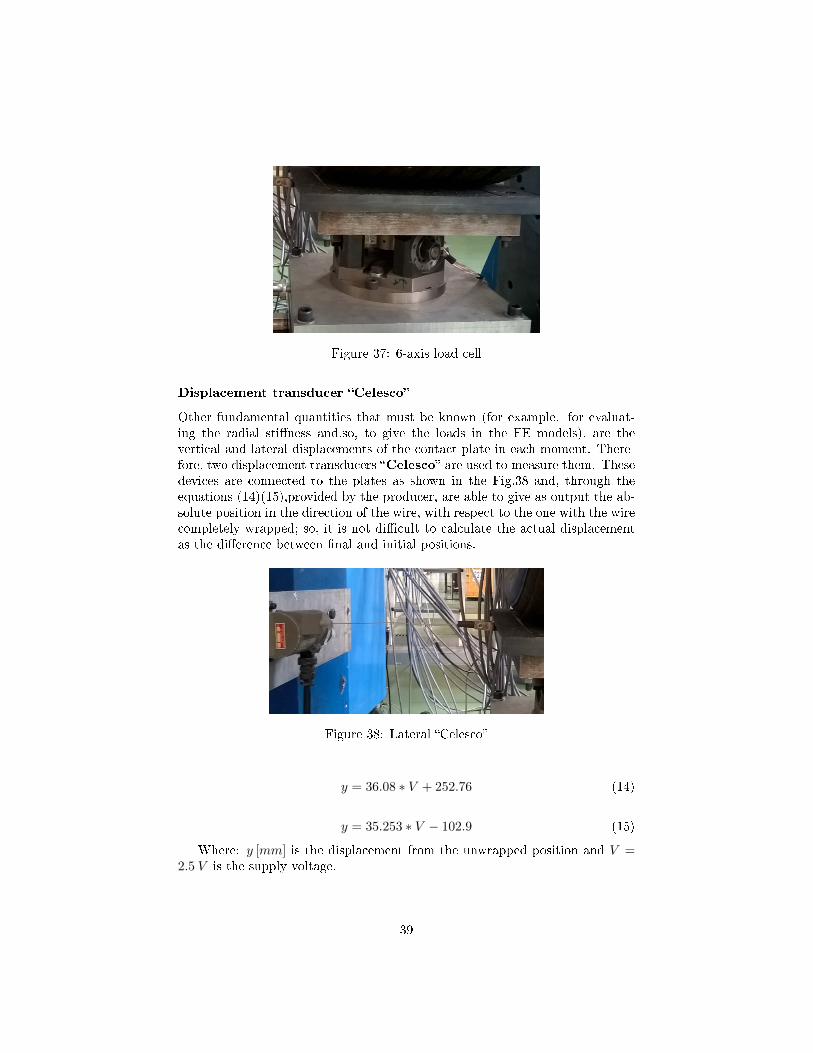
Figure 37: 6-axis load cell

Displacement transducer �Celesco�

Other fundamental quantities that must be known (for example. for evaluat-ing the radial sti�ness and,so, to give the loads in the FE models), are thevertical and lateral displacements of the contact plate in each moment. There-fore, two displacement transducers �Celesco� are used to measure them. Thesedevices are connected to the plates as shown in the Fig.38 and, through theequations (14)(15),provided by the producer, are able to give as output the ab-solute position in the direction of the wire, with respect to the one with the wirecompletely wrapped; so, it is not di�cult to calculate the actual displacementas the di�erence between �nal and initial positions.

Figure 38: Lateral �Celesco�

y = 36.08 ∗ V + 252.76 (14)

y = 35.253 ∗ V − 102.9 (15)

Where: y [mm] is the displacement from the unwrapped position and V =2.5 V is the supply voltage.

39

3.6 Evaluation of the radial sti�ness of the wheel

This paragraph is focused on the evaluation of the radial sti�ness of the wheel.The wheel, during the test is mounted in � position 0° �, that is with the spokeswhere the gauges are placed, oriented perfectly downward; however, it has beenveri�ed that the position does not a�ect the sti�ness of the wheel signi�cantly.Then a radial load is applied to the wheel. This procedure has been repeated fordi�erent in�ating pressures: 4.5 bar, 3.0 bar, 2.5 bar and 2.1 bar. To performthe task, it is necessary to plot vertical forces measured by the cell on the y-axis,as function of the vertical displacement of the plate on the x-axis. The collecteddata are, therefore, processed, considering only the loading cycles, from whenthe contact plate touches the tire, up to the maximum measured force. In theFig.39, the loading cycles of the tested cases are extracted from the completetime histories and plotted together.

Being the measurements linearly distributed, each sti�ness comes from thesimple relation 166:

Krad =Forcerad−final − Forcerad−initial

Displacementrad−final −Displacementrad−initial(16)

In Tab.3, the coordinates of the points are extracted for each pressure caseand the correspondent radial sti�ness is presented, then the di�erent loadingcurves are compared in Fig.39.

Pressure [bar] Initial point Final point Sti�ness [N/mm]

4.5 (323.7 ; 18.42) (346 ; 9918) 443.933.0 (324.2 ; 16.19) (352.4 ; 9724) 344.252.5 (324.6 ; 8.08) (355.4 ; 9341) 303.022.1 (325 ; 31.15) (358 ; 9914) 275.24

Table 3: Loading points and radial sti�nesses

6For being precise the loading curve should be interpolate with a straight line and itsangular coe�cient would give the sti�ness; nevertheless, it comes out from the data that islinear and the procedure can be, therefore, simpli�ed

40

Figure 39: Di�erent loading curves with the evaluated sti�nesses

3.7 Evaluation of the lateral sti�ness of the wheel

The procedure described in sub.3.6 can be used to evaluate also the lateralsti�ness of the wheel. As it comes out from Fig.40, its the lateral behaviour islinear, as well. Therefore the lateral sti�ness is calculated using the followingrelation (eq.17):

Klat =Forcelat−final − Forcelat−initial

Displacementlat−final −Displacementlat−initial(17)

The application of Klat is rather complicated, since it is also a�ected, di�er-ently from Krad, by the actual radial load acting on the wheel. For this reasonit is calculated only for the �Loadcase 1�, which will be later described, at thein�ation pressure of 4.5 bar. The calculation can, however, be done in the sameway for other in�ation pressures or vertical loads.

Figure 40: Lateral displacement- Lateral force curve, in�ation pressure 4.5 bar,Loadcase 1

41

3.8 E�ect of the in�ation pressure on the stress/strainstate of the rim

After the evaluation of the radial sti�ness, the attention is forcused on how thein�ating pressure a�ects the stress/strain state of the rim. This test consistsin in�ating the tire from a pressure of 0 bar to the pressure of 4.5 bar, andmonitoring how the strains vary inside the rim during such a pressure ramp,without any other load applied ( Fig. 41a, 41b, 41c).

(a) E�ect of pressure on S.G. A,B,C,5 (b) E�ect of pressure on S.G. 2,3

(c) E�ect of pressure on S.G. 7,8,9,10,11

Figure 41: Measurements in the di�erent channels under the e�ect of in�atingpressure

The strain induced in each strain gauge by the pressure of 4.5 bar is reportedin the 4. They are all expressed in microstrain7,

7microstrain is µε = [ mµm

] = [mm

× 106]

42

Channel 4µεS.G. A 10S.G. B 2S.G. C -2S.G. 5 8S.G. 2 -69S.G. 3 -79S.G. 7 320S.G. 8 314S.G. 9 308S.G. 10 308S.G. 11 309

Table 4: Strain induced by 4.5 bar in�ating pressure

It can be notice that the maximum in�uence is on the channel, where hightensile strains are induced, while on the spokes the e�ect of in�ating pressureis very low and most of the times negligible. In addition to this, the valuesmeasured in the di�erent strain gauges, follow almost linear path, except for thecases in Fig.41a, where the values are almost negligible. Therefore, to evaluatethe e�ect under di�erent pressures, it is enough to properly scale all these values.

43

3.9 E�ect of radial and lateral load on the stress/strainstate of the rim

This subsection is focused on how the radial and lateral loads a�ect the stress/strainstate of the rim. Di�erent loadcases have been tested using the devices describedin sub.3.4: the in�uence of radial load has been evaluated with di�erent in�at-ing pressure, and those data are used both to calculate the radial sti�ness andto analyze the stress/strain �eld inside the rim. All those measurements havebeen carried out with the wheel in position 0° (i.e. with the spokes with gaugesoriented downward as in sub.3.4). The strain seen by each strain gauge is plot asfunction of time, together with the vertical and lateral force applied in each testthanks to the 6-axis load cell. Then, �xing the in�ating pressure at the valueof 4.5 bar, the test is repeated, this time adding a lateral load to the radialone, whose e�ects have been already observed. This last test has been repeatedat the 5 di�erent positions, to simulate the behaviour of the wheel while it isrotating, getting a su�cient amount of data to carry out also dynamic analysis,since, as written in subs.1.4, the aim of this study is to develop FE models ableto reproduce the stress/strain �eld of the rim, under the e�ect of biaxial load, tomake both static and dynamic analysis faster and easier. At least two loadcasesmeasurements are reported in the Tabs. 5,7,8,9,10, for each wheel orientationlayout: one when it is subjected to a rather low radial load and to a lateral one,and one with an higher radial one is applied, together with the lateral.; theywill be called �Loadcase 1� and �Loadcase 3�, because they are the �rst andthe third loading cycles in the time history. For some of them also a pure radialloadcase has been tested to better understand the in�uence of each e�ect sepa-rately. Some measurements are, in addition to this, used to check the validityof the developed model (sec. 4,5); for them the whole time history is plotted,since, sometimes, values in between the mentioned loadcases are needed.

44

Biaxial loadcase with pressure 4.5 bar and orientation 0°

In Tab.5, the values read in each strain gauge are listed for the 3 loadcases thatwill be used to develop the FE models. For sake of simplicity, from this point onthe will be call Vertical Loadcase, Loadcase 1, Loadcase 3, and these are theirfeatures:

� Vertical Loadcase: in�ating pressure 4.5 bar, vertical load 12990 N

� Loadcase 1: in�ating pressure 4.5 bar, vertical load 5500 N, lateral load3500 N

� Loadcase 3: in�ating pressure 4.5 bar, vertical load 14500 N, lateral load3100 N

Vertical Loadcase Loadcase 1 Loadcase 34µε 4µε 4µε

S.G. A -410 120 -221S.G. B -166 51 -86S.G. C 128 -37 70S.G. 5 -422 65 -281S.G. 2 283 -191 105S.G. 3 212 -222 25S.G. 7 415 330 409S.G. 8 400 321 388S.G. 9 367 310 355S.G. 10 340 300 320S.G. 11 310 292 290

Table 5: Read strains for the analyzed loadcases, orientation 0°

45

(a) Load history (b) E�ect of loads on S.G. A,B,C,5

(c) E�ect of loads on S.G. 2,3 (d) E�ect of loads on S.G. 7,8,9,10,11

Figure 42: Biaxial test, Pressure 4.5 bar, Orientation 0°


� Loadcase 1, 36°: in�ating pressure 4.5 bar, vertical load 6000 N, lateralload 3700 N


46

Loadcase 1, 36° Loadcase 3, 36°4µε 4µε

S.G. A 109 -205S.G. B 32 -138S.G. C -34 62S.G. 5 79 -186S.G. 2 -184 98S.G. 3 -217 16S.G. 7 299 306S.G. 8 304 337S.G. 9 309 370S.G. 10 321 403S.G. 11 337 424


(a) Load history (b) E�ect of loads on S.G. A,B,C,5


Figure 43: Biaxial test, Pressure 4.5 bar, Orientation 36°

47





S.G. A 108 74S.G. B 41 -15S.G. C -32 -26S.G. 5 89 139S.G. 2 -179 -182S.G. 3 -194 -197S.G. 7 304 263S.G. 8 294 253S.G. 9 286 249S.G. 10 287 268S.G. 11 294 296

Table 7: Read strains for the analysed loadcases, orientation 72°



� Loadcase 3, 108°: in�ating pressure 4.5 bar, vertical load 15900 N,lateral load 3000 N

48


S.G. A 52 158S.G. B 27 52S.G. C -15 -51S.G. 5 48 223S.G. 2 -122 -266S.G. 3 -128 -243S.G. 7 319 308S.G. 8 310 288S.G. 9 299 267S.G. 10 294 255S.G. 11 290 245






S.G. A -26 71S.G. B -6 44S.G. C 10 -23S.G. 5 -29 89S.G. 2 -37 -150S.G. 3 -47 -145S.G. 7 324 341S.G. 8 318 329S.G. 9 312 315S.G. 10 310 305S.G. 11 310 296




49



S.G. A -62 -7S.G. B -29 1S.G. C 23 4S.G. 5 -71 -33S.G. 2 6 -19S.G. 3 -6 -37S.G. 7 323 293S.G. 8 317 288S.G. 9 311 283S.G. 10 310 285S.G. 11 310 289


Vertical loadcase with pressure 2.5 bar and orientation 0°

� Vertical loadcase, 180°: in�ating pressure 2.5 bar, vertical load 8750N,

Vertical loadcase, 0°4µε

S.G. A -279S.G. B -113S.G. C 88S.G. 5 -286S.G. 2 206S.G. 3 161S.G. 7 247S.G. 8 235S.G. 9 216S.G. 10 195S.G. 11 174

Table 11: Read strains for the analyzed loadcases, in�ation pressure 2.5 bar,orientation 0°

50

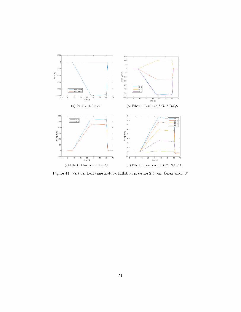
(a) Resultant forces (b) E�ect of loads on S.G. A,B,C,5


Figure 44: Vertical load time history, In�ation pressure 2.5 bar, Orientation 0°

51

3.10 Summary of experimental campaign

In this chapter, it has been shown in details the experiment equipment, showingthe most signi�cant features of each component and the phase of preparationof the experimental bench (subs. 3.3, 3.4, 3.5). After this part, the experimentitself has been presented together with the most important results and dataachieved, which can be brie�y summarized in: the e�ect of the pressure (sub.3.8) and applied loads (sub. 3.9) on the stress/strain state of the rim, and theevaluation of the radial sti�ness of the wheel (sub. 3.6). These results are,as said, very important, since they can allow to understand how the wheel isdeformed, where the most stressed areas are (sub. 5.3) and can be integratedin the development of analytical FE models of the wheel to check their validityby comparing the outputs of the models with the real measured ones or usingthem to set the di�erent material properties of the parts of the wheelset, forexample its radial sti�ness will be used for setting the parameters of the rubberforming the tire (sec. 4, sub. 5.1).

52

4 FE models

This section is focused on the FE models developed to numerically reproducethe stress/strain state of the rim, while a biaxial load (sub.3.9) is provided tothe wheel. The crucial point of this research is to evaluate in detail the tire-riminteraction, that means how the tire transmits the loads to the rim. As input,the magnitudes of the radial and lateral forces are known, and they are appliedthrough a sti� steel plate, to simulate exactly the e�ect of the car own weightand of the friction force that occurs while the car is running into a curve. Thein�ating air pressure, together with the tire itself, withstands the loads andthey both contribute to their transmission to the rim in the bead-bead seatcontact area. However, to simulate how this happens is an hard task and , forthis purpose, di�erent models are suggested, featured by di�erent complexityand precision. At �rst the most complex one, where all the parts are modelledan put together, is shown. For sake of simplicity from this point on it will becalled Complete Model. Then, adapting what has been studied in [6] for amotorbike component to the actual car wheel, another model is suggested. Inthis case, the load is impressed to the tire though the same rigid plate, andthe nodal reaction forces that are generated in the constrained beads are thentransferred on the bead-seats of the rim, whose stress state is analyzed withsuch input forces. This model will be called Intermediate Model. Finally,the loads are put directly on the rim, neglecting the in�uence of tire (and theparameters necessary to its description), which is not present in this case. Theanalysis is much simpler and faster in this case, so this model will be calledSimpli�ed Model.

53

4.1 Complete Model

The aim of this sub-section is to develop an ABAQUS FE-model as close aspossible to the real wheel subjected to radial and lateral load in in-service con-dition. The parameters required to described every di�erent material involved,as also every contact between parts, must be investigated. This aspect mayrepresent the biggest limit of the model since such information is often hard tocollect or not available at all. In addition to this fact, its computational time isthe longest between all the models developed, because of its the huge numberof nodes and highly non-linear material involved. Therefore, a very powerfulcomputer must be used to perform such a simulation.

4.1.1 Rim

The 3-D model of the rim has been provided directly by the OEM and it hasbeen imported in ABAQUS as an IGES �le. Its dimensions and geometry areexactly the same real component used in the experimental campaign 3. It is theexact 3-D of the real component: as shown in Fig. 45, it is very detailed witha lot of curvatures and narrow �llets.

Figure 45: Model of the rim

As it is symmetric, in order to reduce the computational time, it has beensectioned along a vertical symmetry plane, and just half of the part is considered.Then, its surface has been partitioned in the locations of the strain gauges (seesub. 3.5). The dimensions of the highlighted partitions are exactly the same ofthe bases of the gauges (Fig.32, 33, 46), to get the more realistic value possible.

54

(a) Partition S.G. 2,3 (b) Partition S.G. 7,8,9,10,11,5, A-B-C

Figure 46: Particulars of half-rim where the strain gauges partitions are visible

The aluminium alloy rim is completely made of the alloy AlSiMg7, as toldby the manufacturer. As in this test only small deformations occur, for whatconcerns the rim, to de�ne the material properties, it is enough to set the YoungModulus (E) and the Poisson ratio (ν):

EAlSiMg7 = 73GPa νAlSiMg7 = 0.33

Figure 47: Picture of the meshed assembly

Since this part is very detailed with sharp �llet and complicated geometry, itis partitioned using quadratic tetrahedron elements (type C3D10)8, followinga free meshing technique, that is the only possible solution (Fig.48 ).

8For more detailed theoretical information about �nite elements see [16]

55

Figure 48: C3D10 tet. element

The seed size is assigned for having an as regular as possible mesh, butnot being too small at the same time, otherwise the computational time wouldincrease a lot; so, a seed of 6.5 mm has been assigned to the whole part, butthe strain gauge spots, where there are 1.5 mm seeds. The mesh is, therefore,thicker in the strain gauges sites, since in those areas more points are needed tocompute the average strain, comparable with the experimental measurements.(Fig. 47, 49)

Figure 49: Particular of the rim with a thiker mesh in the S.G. areas

4.1.2 Tire

The tire model has been created using the sweep extrusion technique. The sec-tion has been drawn following the geometry of the provided component (Fig.25),then it has been imported in a CAD software and, �nally, it has been extrudedalong a semi-circunference path. The tread pattern has been, therefore, simpli-�ed, maintaing just the 4 main circunferential grooves, in order to have a moreregular mesh, which will allow better results and a lower computational time.Then partitions are introduced in the pro�le sketch and,then, extended to thewhole 3D model by means of sweep for, basically, two purposes:

56

� To allow the use of di�erent materials for the di�erent sections of the tire(for example the rubber used for manufacture the tread is di�erent fromthe one used for the sidewall).

� To have a regular mesh, expecially in the spots closed to curved pro�les.

Figure 50: Tire pro�le

The tire is a very complex sub-system, made of various material with theirown orientations, interacting with themselves. Since this model must reproducethe component in the most realistic way possible, all the di�erent plies havebeen considered. Fig.51 shows the FE model of the tyre and the structuralcomponents are highlighted. The tire beads and the rubber structure have beenmodeled by homogeneous material. The rubber structure is divided in threemain parts, namely the sidewall, the undertread and the tread. A Mooney-Rivlin model has been employed for describing the rubber material property.For the sidewall and the undertread the same parameters have been employed.Tire reinforcements have been included and modelled by means of rebar layersembedded in the tire carcass. A 90° textile body ply was embedded in the wholecross section and a 20 degree steel belt was added in the tire tread. Referencevalues available in the licterature [16, 21, 22] have been considered for materialparameters and for the geometric properties of the reinforcements. In sub.5.1,the radial sti�ness of the wheel FE model will be compared with the one of thereal component (see subs.3.6) for checking the validity of the assigned materialproperties. Tab. 12, 13 summarize the material properties and the geometricproperties of the sections and reinforcements respectively.

57

Figure 51: FE model cross section where all parts are highlighted

Material type Value

Bead Isotropic E = 210GPa ν = 0.30° ply Isotropic E = 210GPa ν = 0.390° ply Isotropic E = 5GPa ν = 0.4

Sidewall and Undertread Mooney-Rivlin C10 = 0.14MPa C01 = 0.43MPaTread Mooney-Rivlin C10 = 0.80MPa C01 = 1.80MPa

Table 12: Material properties of the tire structure ( from [21, 22])

Distance between wires Area per wire

±20° ply 1mm 0.20mm2

90° body ply 1mm 0.40mm2

Table 13: Geometric properties of reinforcements (from [21, 22]).

This part is meshed using linear hexahedron elements (type C3D8RH),following a sweep meshing tecnique (Fig.52)9.


58

Figure 52: C3D8 hex. element

The seed size and the previously created partitions are aimed to have an asregular as possible mesh, but not being too small at the same time, otherwisethe computational time would increase a lot and convergence problems mayoccur (Fig. 53).

Figure 53: Half-section of the meshed tire

4.1.3 Assembly, Interactions and Constraints

The rim and the tire are put together in an assembly and coaxially placed. A3-D rigid planar surface has been created to simulate the very sti� (compared tothe tire) rough steel plate for the transmission of di�erent loads and it is addedto the assembly, perpendicular to the symmetry plane and far enough from the

59

center of the wheel (that is also the origin of the global C-SYS) for not to haveinteraction with other parts in the initial phase (Fig. 54). It is meshed usingwide linear quadrilateral elements (type R3D4), following a structured meshingtechnique (Fig.47).

Figure 54: Assembly

Then, all the interaction between surfaces are de�ned to avoid the materialcompenetration and generate friction in the contact areas:

1. Contact without friction between the bead and the bead seat10 (Fig. 55a)It avoids the compenetration between the tire and the rim in radial direc-tion. No friction is assigned to this area to allow the relative slip betweenthe parts in the in�ating phase. Even if in the real case friction is present,and so a force is generated there, in this model the friction is located onlyin the rim �ange; this should not a�ect the results because all the forcein axial direction generated by the air pressure is, anyway, retained bythe contact with the �ange. A Surface-to-Surface contact with normalbehaviour and a no friction coe�cient is used.

2. Contact with friction between the sidewall and the rim �ange (Fig. 55b)It avoids that the beads go beyond the rim �ange, maintaining the airpressure inside the tire. It is a Surface-to-Surface contact with both normaland tangential behaviour and a friction coe�cient µ = 0.5, which is enoughfor this purpose.

10In Fig. 55a, an interference between the tire and the rim is present, therefore, it will beremoved during the �rst simulation step, when the beads are moved inward to avoid possiblecomputational errors due to this aspect.

60

3. Contact with friction between the rigid plate and the tire (Fig. 55c)It avoids the compenetration between the plate and the tire, allowing theload transmission. It is a Surface-to-Surface contact with both normaland tangential behaviour and a friction coe�cient µ = 1.2, which repro-duces the friction with the rough plate, which is comparable with the onebetween tire and asphalt.

(a) Surfaces involved in contact 1 (b) Surfaces involved incontact 2

(c) Surfaces involved in contact 3

Figure 55: Contact surfaces

During the experiment the wheel was bolted in the 5 holes of the hub; thisgenerates an encastre. To reproduce this constraint, the surface in contact withthe �ange is coupled with the reference point RP1, and all the 6 degrees offreedom of RP1 are constrained. A similar procedure is used also for moving tothe planar surface against the tire, in fact it is rigidly coupled with a referencepoint RP placed in its center and the desired desplacement is easily applied toit. In addition to this, considering just half of the wheel, symmetry constraintsmust be applied in the surfaces sectioned by the symmetry plane. Fig. 56

Figure 56: Assembly picture, where RP and constrains are highlighted

61

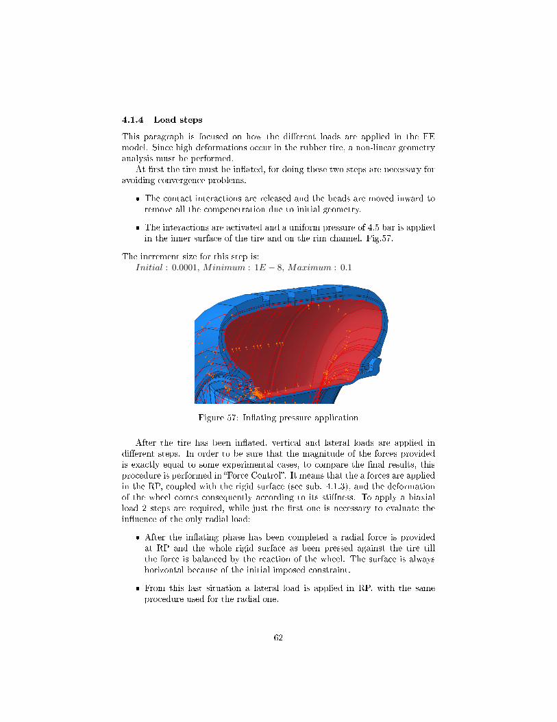
4.1.4 Load steps

This paragraph is focused on how the di�erent loads are applied in the FEmodel. Since high deformations occur in the rubber tire, a non-linear geometryanalysis must be performed.

At �rst the tire must be in�ated, for doing these two steps are necessary foravoiding convergence problems.

� The contact interactions are released and the beads are moved inward toremove all the compenetration due to initial geometry.

� The interactions are activated and a uniform pressure of 4.5 bar is appliedin the inner surface of the tire and on the rim channel. Fig.57.

The increment size for this step is:Initial : 0.0001, Minimum : 1E − 8, Maximum : 0.1

Figure 57: In�ating pressure application

After the tire has been in�ated, vertical and lateral loads are applied indi�erent steps. In order to be sure that the magnitude of the forces providedis exactly equal to some experimental cases, to compare the �nal results, thisprocedure is performed in �Force Control�. It means that the a forces are appliedin the RP, coupled with the rigid surface (see sub. 4.1.3), and the deformationof the wheel comes consequently according to its sti�ness. To apply a biaxialload 2 steps are required, while just the �rst one is necessary to evaluate thein�uence of the only radial load:

� After the in�ating phase has been completed a radial force is providedat RP and the whole rigid surface as been pressed against the tire tillthe force is balanced by the reaction of the wheel. The surface is alwayshorizontal because of the initial imposed constraint.

� From this last situation a lateral load is applied in RP, with the sameprocedure used for the radial one.

62

The increment size for these steps is:Initial : 0.01, Minimum : 1E − 7, Maximum : 0.1

4.1.5 Simulated loadcases

Following these simple steps 3 loadcases are simulated, which can be directlycompared with the available experimental data (see subs. 3.9):

1. Vertical Loadcase, 4.5 bar, 0°: in�ating pressure 4.5 bar, verticalload 12990 N, orientation 0° (i.e. with the spoke where the gauges areapplied placed downward)

2. Loadcase 1, 4.5 bar, 0°: in�ating pressure 4.5 bar, vertical load 5500N, lateral load 3500 N, orientation 0° (i.e. with the spoke where thegauges are applied placed downward)



Of course the magnitude of the loads has to be divided by two since half wheelhas been considered.

63

4.2 Intermediate model

This FE model is built adapting what has already been studied in [6], for whatconcerns the numerical analysis, to the considered car tire and rim. It hasnamed �Intermediate� since the analysis is not as complex as the one describedin subs. 4.1, being the components studied separately, as it will be shown. Lessinformation and computational time are required. However, also in this casethe mechanical characteristics of the rim and, above all, of the tire must beknown. This fact may represent a limit, because, as said, the knowledge ofthese parameters (for example the rubber features) and data, sometimes, mayrequire a lot of time or it may not be possible at all. In addition to this, all theoutputs of each steps must be carefully processed before they could be appliedto the following one and allow, in this way, the proceeding of the simulation.For example some time must be spent to get the reaction forces in the beads,sum them up in each set of node and translate them on the rim (subs.4.2.2).For these reasons, in the following subs.4.3, a simpler model, with less inputsrequired, will be developed again.

4.2.1 Parts

The tire and rim properties and geometry used in this model are the same ofthe ones described in subs. 4.1.1, 4.1.2. The descriptions of the components andall the parameters involved in their characterization can be, therefore, found inthose sub-sections. Since the computational time is smaller in this case, thewhole components are considered instead of their half. To provide the radialand lateral loads to the tire, the same rigid plate, whose properties are listedin subs. 4.1.3, is used. However, a sligthly di�erent approach is followed inthis case to get, at last, the stress/strain �eld inside the rim caused by bothbiaxial and radial loads. The procedure is described in detail in the followingsub. 4.2.2.

4.2.2 Load steps

In�ation pressure

The �rst simulation consists in the in�ation of the tire. A 2-D axisymmetricFEM model is built for this purpose from the section experimentally obtained.Its geometry, layers and material properties are the same of the previouslydescribed 3-D �Complete Model�. The cross section of the tire is constrainedat the tire-rim interface and a uniform in�ating pressure is applied at the innersurface. During this step the position of the constrained surface can translatelaterally, till its displacement is equal to the rim �ange width (see Fig. 58).Therefore, once the in�ation pressure is applied, it undergoes some seformationtill it reaches its �nal deformed shape.

64

Figure 58: Tire 2-D model, where in�ation pressure and maximum displacementconstraint are applied

Application of radial and lateral loads on the tire

In the following step, after the in�ation procedure has been completed, a 3-Dmodel is generated by extruding the deformed 2-D axisymmetric model (Fig.59)along a circular path.

Figure 59: Tire 3-D model, with the encastre boundary conditions highlighted.

The tire is, then, constrained in the tire-rim interaction surface with anencastre because, once the beads have reached their seats, their movement isfully denied (Fig.59, 60). It is, then, partitioned using the same linear brickelements (type C3D8RH)11, and following a sweep meshing tecnique, as before.It must be underlined, now, that, thanks to the sweep geometry and partitiontechnique adopted, the elements in each section are repeated with the sameshape along the whole circunference. This aspect will be rather helpful to obtain,through a MATLAB code, the reaction forces in radial and lateral directionsalong the tire-rim interface (Fig.61)


65

Figure 60: Tire-rim interaction surface where the encastre is loacated

A uniform pressure is applied on the inner surface and the rigid plate, whosefeatures are the same presented in subs.4.1.3 for the �Complete Model�, is pushedagainst the tire and then laterally pulled, by applying a force in the referencepoit RP, rigidly coupled to the whole plate surface. Its desplacement, as before,depends on the impressed force and on the radial sti�ness of the wheel.

The increment size for these steps is:Initial : 0.01, Minimum : 1E − 7, Maximum : 0.1

Evaluation of the reaction forces in the tire-rim interface and appli-cation of them on the rim

The outputs of interest in the previous step are the nodal reaction forces in theconstrained tire-rim interface. By knowing the layout of the �.dat� output �le,and the orientation of each element of the interface, the nodal reaction forcesare extracted and the resultants in X,Y and Z directions are computed for eachlayer, creating paths as the one shown in Fig. 61. This procedure is, then,repeated for each layer, on both the two beads.

Figure 61: Example of a path where resultant lateral and radial forces arecomputed

Then they are divided per the length of the elements obtaining forces perunit length [N/mm], and, after being converted in polar coordinates, they areplotted to observe their distributions (Fig.62). It is clear that they act on an arc

66

what is wider than ±40° one described in[1]. This consideration will be usefullater, in the development of a simpler FE model (subs.4.3).

Figure 62: Reaction forces per unit length at the tire-rim interface

These forces per unit length are, then, multiplied by the length of the ele-ments of interest of the rim surface. The radial forces are, thus, put on a nodeset located on the bead seats, while the lateral ones on the �anges as suggestedin [6] (Fig. 63).

The model is, for this last step, a fully linear model, since it consists onlyin the aluminium rim, which undergoes only small deformations in the elastic�eld. Also in this case it is encastred by connecting the rear suface of the hubarea to a reference point RP1, whose degrees of freedom are fully constrained(see. Fig. 65).

67

Figure 63: Nodes for the application of the resultant reactions forces on the tirebeads.


Following the previously illustrated procedure, the same loadcases analysed withthe �Complete Model� are simulated, to have a direct comparison between themodels and the available experimental data (see subs. 3.9):





68

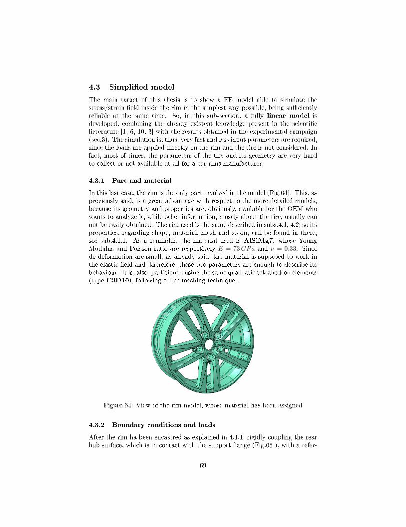
4.3 Simpli�ed model

The main target of this thesis is to show a FE model able to simulate thestress/strain �eld inside the rim in the simplest way possible, being su�cientlyreliable at the same time. So, in this sub-section, a fully linear model isdeveloped, combining the already existent knowledge present in the scienti�clicterature [1, 6, 10, 3] with the results obtained in the experimental campaign(sec.3). The simulation is, thus, very fast and less input parameters are required,since the loads are applied directly on the rim and the tire is not considered. Infact, most of times, the parameters of the tire and its geometry are very hardto collect or not available at all for a car rims manufacturer.

4.3.1 Part and material

In this last case, the rim is the only part involved in the model (Fig.64). This, aspreviously said, is a great advantage with respect to the more detailed models,because its geometry and properties are, obviously, available for the OEM whowants to analyze it, while other information, mostly about the tire, usually cannot be easily obtained. The rim used is the same described in subs.4.1, 4.2; so itsproperties, regarding shape, material, mesh and so on, can be found in there,see sub.4.1.1. As a reminder, the material used is AlSiMg7, whose YoungModulus and Poisson ratio are respectively E = 73GPa and ν = 0.33. Sincede deformation are small, as already said, the material is supposed to work inthe elastic �eld and, therefore, these two parameters are enough to describe itsbehaviour. It is, also, partitioned using the same quadratic tetrahedron elements(type C3D10), following a free meshing technique.

Figure 64: View of the rim model, whose material has been assigned

4.3.2 Boundary conditions and loads

After the rim ha been encastred as explained in 4.1.1, rigidly coupling the rearhub surface, which is in contact with the support �ange (Fig.65 ), with a refer-

69

ence point RP1, whose six d.o.f. are constrained, the loads are applied. This is,undoubtedly, the most interesting aspect of this model, since, as it will be ex-plained in sec.5, how the loads are applied greatly a�ects the stress/strain �eldof the rim. The applied loads are subdivided in 3 di�erent families: pressureload, radial load and lateral load. For being as clear as possible, each onewill be presented in its own paragraph and, meanwhile, a few words are spentabout the evaluation of the loaded arc, as well. This is not just a report layoutmatter, in fact, since the model is fully linear ( and so the superimposition ofe�ects principle is valid), each load can be applied separately and the resultante�ect can be summed at the end, generating the di�erent loadcases of interest.

Figure 65: View of the constrained rim

Pressure load

As it comes out from the experiment in subs.3.8, the in�ation pressure a�ectsthe stress/strain �eld of the rim considerably. To take into account its in�uence,what has been studied in [1, 6] has been considered and adapted to the actualgeometry. The air pressure, pressing on the sidewalls of the tire, pushes thebeads against the rim �anges, generating a lateral load, which is directed in anaxial direction. Considering the pro�le of the cross section of wheel describedin sec.2 and shown Fig.66, the axial component of the force (Wp), which resultsfrom an in�ation of the tire (P0) is calculated using the relations:

Wp = π(a2-r2f )× P0 [N ]

where a is the design radius of the tire, and rf is the radius at the loadingpoint on the rim �ange. Since the axial load is supported by the tread of the tireand the rim �ange, approximately a half of the load is assumed to be loadedonto each part[1].

70

Figure 66: Dimensions involved in in�ation pressure load

Thus, the load on a unit circumferential length of the rim �ange (Tf ) isexpressed as:

Tf =Wp


P0

4Örf[N/mm]

In the real situation all the external surface of the beads is pressed against therim �ange. The exchanged force does not act only on a linear set of nodes. Toreproduce this aspect, the axial contribution of the in�ating pressure is appliedon the whole vertical surface of the rim �ange as a Uniform Pressure (Fig.67); therefore, the previous formulation has been slightly modi�ed in:

Pf =Wp


P0

4Örf × hf[MPa] (18)

where rf is now the average radius of the loaded circular sector of the �angeand hf is its height.

Figure 67: Pressure lateral load on the rim �ange.

71

However, the in�ation pressure acts on the outer surface of the rim channel,too; this time it acts directly on it. It is, therefore, applied on the whole outerpart of the rim again as a Uniform Pressure (Fig.68).

Figure 68: Surface where in�ating pressure acts directly

Following this procedure, two cases are simulated:

� In�ation pressure of 4.5 bar

� In�ation pressure of 2.5 bar

Loaded arc evaluation

What is developed in this subsection gets some ideas from[1, 6] and revisitsthem in order to obtain a stress/strain �eld as closed as possible to the real onefrom experimental measurements (sec.3).

In both the articles the load has been, reasonably, applied in the bead seats;so, this procedure is followed also here. However, the arcs which the loadsact on are di�erent: in [1] an arc of ±40° has been suggested, while it has beendemostrated in [6], from both an analytical and numerical point of view (Fig.13),that the forces are distibuted on a wider arc. Therefore, a simple procedure isdeveloped for calculating the best arc on which to apply the loads. Consideringa wheel, where the tire has a radius a and a rim, with the bead seats located ata distancerb from the center (Fig.69). After the application a force, by pressinga plate against the tread, the tire undergoes a deformation, and the lateralprojection of its print is called ltire. The maximun displacement takes place inthe central contact point and it is named drad.

72

Figure 69: Lateral schematic view of the wheel, useful to calculate the loadingarc

ltire is, then, projected on the bead seat circunference, and the angle in thecenter that de�nes such a chord is the actual load angle, from this point oneach symmetric half will be called θ, and the arc it describes is the arc ±θ. It,therefore, depends on the applied radial load and on the radial sti�ness(that can be easily obtained for example using Pacejka's �Magic Formula� [7])of the wheel, which is the only parameters necessary for setting the model. Theadvantages of such a model are, then, evident.

The radial sti�nesses for the simulations are taken from the one obtainedfrom the experiment (subs.3.6):

Krad4.5 = 443.93 [N/mm]

Krad2.5 = 303.02 [N/mm]

The displacement is, then, calculated:

drad =Force

Krad[mm] (19)

The half angle in the center of the circunference of radius a is:

θa = arccos(a− drad

a) (20)

The length ltire can be obtained with the �Chord Theorem�:

ltire = 2a× sin(2θa2

) (21)

From this each half of the load angle, θ0 is:

73

θ0 = arcsin(ltire/2

rb) (22)

The values obtained strictly following this procedure are, then, increasedof about 20%, since it has been observed (sub.5.1) that the loads are, oth-erwise, concentrated too much on the spokes inside the arc, giving too highstrains/stresses. Both the experimental results and [6] con�rm that the tire dis-tribution action is wider than what comes out of this mathematical formulation.

For the di�erent loadcases analyzed the following arcs are, therefore, used:

� Pressure 4.5 bar, high loads ( > 12900 N), θ0 = ±50° (Fig.70)

� Pressure 4.5 bar, low loads (5500 N), θ0 = ±30°

� Pressure 2.5 bar, load 8750 N, θ0 = ±45°

Figure 70: View of the rim where the arc ±50°is highlighted on the bead seatand on the �ange

Radial load

In [1] the radial load is applied by mean of a distibuted cosine function on thearc of interest. On each element, a nodal force, that is parallel to the directionof the resultant force, is acting (Fig.8). Since in [6] such a load is supposed toact in radial direction, this load is applied using a Pressure on the bead seats.For de�nition, in ABAQUS, a pressure is perpenducular to surface which it actson (Fig.71).

74

Figure 71: Radial load applied on the inner and outer beas seats

The magnitude of the load follows a cosine distribution, which is simplyimplementable through an Analytical Field. Its formulation comes from [1]and it is adapted to the actual case so that it could take into account the di�erentdirection pf the distributed force.

From 3 the pressure in each point, that depends on its angular position θ:

Wr = W0 × cos(π

2

θ

θ0

)[MPa] (23)

Where W0is the maximum amplitude of the pressure.By knowing W , which is the total load applied, W0 can be easily calculated

in MATLAB, using symbolic variables, from:

W = b

θ0ˆ

−θ0

W0 × rb × cos(π

2θ0θ)× cos(θ)× dθ [N ] (24)

Where b is the width of the bead seats and rb, as said, is its radius.OnceW0has been evaluated for each di�erent loadcase, eq.23 is implemented

in ABAQUS, using the formulation:

Wr = W0 × cos(π

2

atan(X/Z)

θ0

)[MPa] (25)

Where X is the horizontal coordinate in the rim plane and Z is the vertical onein the global reference system (global C-SYS) located in the center fo the part.For the cases with di�erent wheel orientation an additional C-SYS must becreated, having the same origin of the global one but properly rotated (Fig.72).

75

Figure 72: View where the C-SYS used in the Analytical �eld is highlighted

Lateral load

Both the common sense and [6] suggest to apply the lateral load on a nodeset located on the rim �ange. Since in Fig.13, the radial and axial loads havemore or less the same distributions and act on a similar arc, the axial load isapplied as a Pressure on the same �ange surface where the lateral componentof in�ating pressure is acting. However it acts just on the arc calculated fromeq.22 with the actual radial force (Fig.70), and for reproducing its distributionin the simplest way possible, the same cosine function, implemented throughthe same Analytical �eld (eq.23), is adopted.

Figure 73: Lateral loads acting on the inner and outer �anges


Because of the simplicity of the model and its short computational time, di�erentloadcases are simulated, in order to have a wide number of results to comparewith the other developed models and with the available experimental data:


76



4. Loadcase 1, 4.5 bar, 36°: in�ating pressure 4.5 bar, vertical load 5970N, lateral load 3700 N, orientation 36° (with respect to the position 0°)

5. Loadcase 3, 4.5 bar, 36°: in�ating pressure 4.5 bar, vertical load15600 N, lateral load 2700 N, orientation 36° (with respect to the po-sition 0°)


77

5 Analysis of results and comparison among mod-els

This chapter is dedicated to the analysis of the outputs of the di�erent models.They are compared with the experimental data collected and organized in sec.3.At �rst the procedure adopted to check the validity of the material propertiespreviously assigned in ABAQUS is shown (sub.5.1 ). The radial and lateralsti�nesses are calculated and compared with the real ones, coming from theexperiment. Then, the outputs of the simulation are analyzed and the strainsmeasured in the strain gauges spots are collected and compared with the ex-perimental data of the same loadcases. Some considerations are, at last, doneabout the advantages and disadvantages of each model. The main achieved goalcan be the good reliability of the �Simpli�ed Model�. In most of situations, itcan be easily implemented, making the design phase faster and easier.

5.1 Validation of assigned material properties

Comparison between real and simulated sti�nesses

The check, performed to verify that the assigned material properties are reliable,consists in the radial sti�esses calculation and comparison between the wheelmodelled in ABAQUS (descrived in the 'Complete Model' subsection 4.1) andthe one really tested in the lab (subs.3.6). The procedure is rather simple: inboth the cases the radial force impressed to the contact plate (on the y-axis) isplotted as function of the radial displacement of the plate itself (on the x-axis),after the contact with the tire (Fig.61). In the case of the experiment the forcescome directly from the 6-axis load cell placed below the steel contact plate,while in the FEM it is read as a reaction force in the only constraint point RP1(4.1).

Figure 74: Example of a radial displacement of the tire-plate contact point inthe 'Complete Model'

78

Figure 75: Example of vertical reaction force

The points on the curves in this way obtained, which are in all the caseslinear, are interpolated and the angular coe�cient represents the radial sti�nessof the wheel.

Figure 76: Loading curves in the di�erent cases

The sti�nesses are, then, listed in Tab.14, in order to do a direct comparison:

79

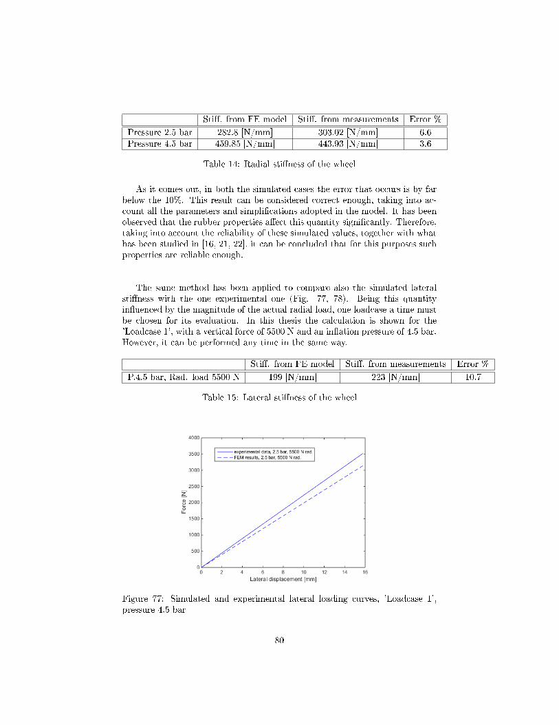
Sti�. from FE model Sti�. from measurements Error %

Pressure 2.5 bar 282.8 [N/mm] 303.02 [N/mm] 6.6Pressure 4.5 bar 459.85 [N/mm] 443.93 [N/mm] 3.6

Table 14: Radial sti�ness of the wheel

As it comes out, in both the simulated cases the error that occurs is by farbelow the 10%. This result can be considered correct enough, taking into ac-count all the parameters and simpli�cations adopted in the model. It has beenobserved that the rubber properties a�ect this quantity signi�cantly. Therefore,taking into account the reliability of these simulated values, together with whathas been studied in [16, 21, 22], it can be concluded that for this purposes suchproperties are reliable enough.

The same method has been applied to compare also the simulated lateralsti�ness with the one experimental one (Fig. 77, 78). Being this quantityin�uenced by the magnitude of the actual radial load, one loadcase a time mustbe chosen for its evaluation. In this thesis the calculation is shown for the'Loadcase 1', with a vertical force of 5500 N and an in�ation pressure of 4.5 bar.However, it can be performed any time in the same way.

Sti�. from FE model Sti�. from measurements Error %

P.4.5 bar, Rad. load 5500 N 199 [N/mm] 223 [N/mm] 10.7

Table 15: Lateral sti�ness of the wheel

Figure 77: Simulated and experimental lateral loading curves, 'Loadcase 1',pressure 4.5 bar

80

(a) Only Infating Pressure

(b) Radial + Lateral loads

Figure 78: Particular of the wheel deformation under lateral load, �CompleteModel�

Also in this case the absolute error committed, with respect to the real value,is about 10 %. It is considered reliable enough and it con�rms, another time,that the assigned material properties are correct for this application.

81

5.2 Analysis of the stress/strain �eld on the wheel

E�ect of the di�erent loadcases

After each model has been set, the simulations are performed. The computa-tional time, as said, is much longer in the 'Complete Model' and 'IntermediateModel', with respect to the 'Simpli�ed' one, which is fully linear and easy toset. This is undoubtedly a great advantage of it.

So, the strains (E) in strain gauge spots, which have been previously par-titioned on the rim surface (subs. 4.1.1), are read for the di�erent loadcasespresented in sec.4. Of course, in each comparison the rim must be subjected tothe same loads in all the models used as, also, in the experiment.

The procedure is simple: in each partition a local Coordinate System (C-SYS), whose x-axis is parallel to the respective strain gauges measurementdirection, is placed (Fig.79).

Figure 79: Local C-SYS

Then, for each gauge, the whole strain �eld is transformed following the localreference system and the strains in the x-direction (E11) of the surface nodesunder the strain gauge base are averaged (Fig.80 ), getting, �nally, the actualoutputs that can be compared with the experimental collected data. For thestrain rosette 2 reference systems are used: one orientated as A, which allowsalso to get the C strain by reading E22, and one directed as B, that is rotated45° with respect to A direction.

82

Figure 80: Strain E11 on a strain gauge base

The procedure is repeated for each strain gauge site, getting, in this way,a rather clear view of the strain �eld of the component. These results, forthe di�erent loadcases, are then reported in the Tables 16, 17, 18, 19, 20, 21,together with the values coming from the experiments, in order to facilitate thecomparisons (sub.5.3). All the results are expressed in microstrain12.

12microstrain is µε = [ mµm

] = [mm

× 106]

83

Experimental Simpli�ed Model Intermediate model Complete Model

est 2 283 411 319 304est 3 212 311 231 218est 7 415 454 413 419est 8 400 442 404 410est 9 367 412 381 387est 10 340 367 351 357est 11 310 314 320 326est 5 -422 -555 -462 -454A -410 -527 -440 -436B -166 -164 -206 -143C 128 127 108 99

Table 16: Vertical loadcase, Pressure 4.5 bar, orientation 0°

Experiment Simpli�ed Model Intermediate model Complete Model

est 2 -191 -97 -147 -185est 3 -222 -148 -205 -239est 7 330 374 355 348est 8 321 364 351 344est 9 310 339 342 336est 10 300 315 332 328est 11 292 300 322 318est 5 65 -25 12 40A 120 43 81 103B 51 24 35 30C -37 -10 -20 -26

Table 17: Loadcase 1, Pressure 4.5 bar, orientation 0°

84

Experiment Simpli�ed Model Intermediate model Complete Model


Table 18: Loadcase 3, Pressure 4.5 bar, Orientation 0°

Experiment Simpli�ed Model

est 2 -184 -107est 3 -217 -158est 7 299 298est 8 304 317est 9 309 347est 10 321 378est 11 337 384est 5 79 20A 109 27B 32 -18C -34 -14


85

Experiment Simpli�ed Model

est 2 98 198est 3 16 100est 7 306 309est 8 337 361est 9 370 407est 10 403 442est 11 424 448est 5 -186 -269A -205 -311B -138 -46C 62 61


Experiment Simpli�ed Model Intermediate Model Complete Model


Table 21: Vertical Loadcase, Pressure 2.5 bar, Orientation 0°

86

E�ect of the in�ation pressure

Using the �Simpli�ed Model�, which is a fully linear model, the e�ects of thedi�erent loads have been applied separately and, then, summed up. Therefore,considering only the in�ation pressure e�ect on the strain �eld of the rim, a com-parison can be done between the simulated and the measured values (Tab.22),being the data already available for both the cases:

Experimental Numerical

est 2 -69 -58est 3 -79 -69est 7 320 347est 8 314 347est 9 308 347est 10 308 349est 11 309 349est 5 8 8A 10 9B 2 4C -2 -3

(a) 4.5 bar

Experimental Numerical

est 2 -38 -31est 3 -44 -38est 7 178 195est 8 175 195est 9 171 195est 10 171 195est 11 171 195est 5 4 2A 5 4B 1 2C -1 -1

(b) 2.5 bar

Table 22: E�ect of in�ation pressure, using �Simpli�ed Model�

Like in the previously analyzed cases, the strains are correctly simulated bythe model. The error committed is very low and this is an additional proof ofthe validity of the developed model. Therefore, for lots of application this is thebest tradeo� between precision of results and simplicity of implementation.

Analysis of results

Considering all the presented results, some considerations about the stress/strainstate of the wheel can be done.

When the wheel is in position 0°, for every di�erent loadcases, a radial loadintroduces some tension on the outer surface of the spokes (read by the straingauges 2 and 3) and some compression on the inner one (read by the straingauges 5, A and B), along the spoke direction. On the other hand the lateralone, which is pulling the rim outward, has an opposite behaviour. In fact theabsolute values read by s.g. 2, 3, 5, A, B, and C are, always, smaller whena biaxial load is applied wit respect to the case of purely radial load. Thepredominance of one or the other, depends on the magnitudes of the appliedloads and cannot be easily guessed before the analysis has been performed. Thee�ect of radial load on the measured spokes is supposed to be lower as the wheelis rotated. Both considering the values listed in Tab.20, for the position 36°, andthe deformed shape of the wheel (Fig.81), the magnitude of the read strains is

87

lower than the ones read in position 0°. This trend continues till the situation isreversed far away from the loading arc in horizontal position, where the spokesbehave in an opposite way. In this last case to undestand the in�uence of lateralload is not easy and a simulation must be carried out.

(a) Displacement in radial direction,U3

(b) Displacements in lateral direction, U2

Figure 81: Deformed shape and displacements due to radial load

88

Regarding the rim channel, looking at the results listed in Tab.22, it can beconcluded that the tensile strains read by the strain gauges 7, 8, 9, 10, and 11are mostly due to the in�ation pressure, which acts directly on the rim outersurface and indirectly on the rim �ange, by pushing the beads against it. A smalltensile contribution is added by the radial load, whose magnitude is decreasinggetting far from the vertical axis, as shown in both the cases at 0° and 36°. Thee�ect of lateral load is minimum and it is limitated to small compressive strainsinside the loading arc.

It is also important to spend a few words about the loading arc width.The procedure described in sub.4.3, is developed taking into account what hasbeen studied in [1, 6]. Nevertheless, using the �Simpli�ed Model�, it has beenobserved that the values are getting worse and worse as the arc is di�erentfrom the calculated one. If it is less wide the strains on the spokes are moreoverestimated, getting far from the real ones. On the other hand, if it is bigger,the the values read on the rim channel follow a wrong distribution: they arebigger far away from the vertical axis than near it. This can lead to a wrongevaluation of the deformed shape and of the stress �eld of the rim. To con�rmthis fact, the case with the orientation at 36° is simulated, as well. The behaviourof the wheel is the same. Therefore, it can be concluded that, using such a simplemodel, with such a load distribution, the procedure for calculating the loadingarc is the best possible choice.

5.3 Comparison between models

The Tables presented in sub.5.2 allow to compare the di�erent models betweeneach other.

Those values tell immediately that the �Complete Model� and �IntermediateModel� outputs are very reliable for what concerns the strain �eld evaluationinside the rim. In all the simulated loadcases, with in�ation pressure of 4.5 and2.5 bar and with both radial and biaxial load, the absolute error committedwith respect the experimental measurements is lower than 10 %. Therefore,if a very precise analysis is required, both of them can be used, provided thatall necessary information (like for example the tire structure, geometry andmaterial properties) are known and a powerful computer in available, since thesimulation can be rather heavy from a computational point of view.

If, for any reason, they cannot be implemented, for example the tire prop-erties are not known, or a su�ciently powerful hardware is not available, or,simply, a faster and easier analysis is needed, the �Simpli�ed Model� is the onlypossible choice.

However, in this last case, the stresses/strains are slighty overestimated, tilla maximum of 30 % in some points on the spokes, while on the rim channelthe values are very close to the real ones, sometimes even closer than the onesobtained with the more complex models. Considering that the time required forsetting the model and performing the simulation is negligible with respect to themore realistic cases, the �Simpli�ed Model� is the best model to reproduce thestress/strain �eld of the wheel in most of common applications. This justi�es

89

the detailed research around it and it can be easily adopted to simulate the testdescribed in sub.2.3.

The �Simpli�ed Model�, however, as it comes out for example from Tab.16,overestimates mosty the e�ect of radial loads. The simulation of situationslike Loadcase 1 (Tab.17), where lateral and lateral load are small in magnitudeand comparable between each other, can lead to an underestimation of thetotal stress/strain �eld on the surface of the spokes. However, in this case thestress/strain magnitude is very small and this should not constitute a problem.For more severe loadcases, to which the component is supposed to resist, it ismore restrictive than other models.

The comparison between real and simulated values allows, also, to be con-scious of the reliability of the outputs during the design of the wheel or theoptimization of its shape.

90

6 Conclusions

The analysis of the stress/strain state of the automotive alloy wheel, founda-mental in the design phase, is a very hard task. It has a complicated geometryand it has to withstand di�erent loads. Therefore, it is performed through someexpensive and time-consuming experimental tests or through rough calculations.The development of accurate models will provide advantage in terms of moneyand time saving. Three di�erent numerical models for simulating the stressstate on the rim under the e�ect of combined vertical and lateral loads, havebeen developed.

1. The �Complete Model� is made up of of the rim, coupled with the tire ina single assembly. The simulation consists in various steps: at �rst thetire is in�ated by adding a pressure on its inner surface and on the outerrim channel. The vertical and lateral loads are, now, applied to the wheelby radially pushing a rigid plate against the tire and, then, by pullingit axially. In this model there are a lots of nodes and highly non-linearmaterials. The computational time of the simulation is, therefore, verylong. In addition to this, a lots of parameters, not always available, arerequired to set it.

2. In the �Intermediate Model�, the behaviour of the tire and of the rim is an-alyzed separately. The in�ation phase is performed on the axial-symmetricmodel of the tire. The 3D of the part is generated by sweep extruding the2D defomed shape. It is, then, encastred in the beads. The radial andlateral loads are applied using the same rigid plate mentioned before. Thenodal reaction forces are computed and, in a second step, translated to thebead seats. The stress/strain �eld of the rim is, �nally, obtained thanksto a fully linear simulation of the so-loaded part. The computational timeis lower than the �Complete Model�; however, a more detailed process-ing of the intermediate results is required. All the parameters needed tocharacterize tire and rim must be known, as well.

3. The �Simpli�ed Model� involves only the alloy rim. The load generatedby the in�ation pressure is applied using a uniform pressure on the �angesand on the rim outer surface. For the vertical and lateral loads a pres-sure, distributed as a cosine function on a calculated loaded arc, is used.The model is very easy to set and a few parameters are required: it issu�cient to have a CAD of the wheel, to know the elastic properties ofthe aluminium, to roughly estimate the radial sti�ness of the wheel andto know the magnitude of the applied loads. The computational time isnegligible compared to the other two models.

An experimental bench is built to reproduce the simulated loadcases. Somestrain gauges are placed both on the rim channel and on the spokes. Themeasured strains are, then, compared to the simulated ones to check the validityand accuracy of the models.

91

Using the �Completed Model� and �Intermediate Model� the error committedis, in any case, lower than 10 %. So, provided that all the parameters andinstruments required by such simulations are available, the actual stress/strain�eld of the rim can be estimated in a very precise way. Their implementation isnot always possible; so a �Simpli�ed Model� is developed, as well. It sometimesoverestimates the actual strain state of the rim, till a maximum of 30 % in somepoints the spokes, while on the rim channel may be even more accurate thanthe other two. Nevertheless, in most of common applications, this last model isthe best choice. In fact, the �Simpli�ed Model� represents in most of situationsthe best trade o� between computational time and required parameters on onehand and reliability of results on the other.

In conclusion, if a manufacturer wants to achieve very high-performancecomponents, he should spend more time and money implementing one of themore detailed models. Otherwise, using the simplest one, a reliable and correctanalysis can be equally performed in a cheaper and easier way, by taking intoaccount the error committed in the safaty coe�cient de�nition. However, inall the cases, lots of money and time can be saved using FE analysis thanexperimentally testing a real wheel.

92

References

[1] Stearns J, Srivatsan T, Prakash A, Lam P (2004) Modeling the mechani-cal response of an aluminium alloy automotive rim. Materials Science andEngineering

[2] Road and O�-Road Vehicle System Dynamics Handbook; GianpieroMastinu, Manfred Ploechl

[3] Samuel Onoriode Igbudu, David Abimbola Fadare. Comparison of LoadingFunctions in the Modelling of Automobile Aluminium Alloy Wheel underStatic Radial Load. Scienti�c Research Publishing, 2015.

[4] V. Grubisic, Automotive Wheels: Method and Procedure for Optimal De-sign and Testing, SAE Technical Paper, Series no. 830-135, 1983, p. 20.

[5] Ballo F, Gobbi M, Mastinu G, Previati G, Zerboni R (2015) Motorcycletire modeling. In: Proc. of the ASME 2015 IDETC/CIE 2015, Boston,Massachussetts, USA

[6] Gobbi M, Ballo F, Mastinu G, Previati G (2016) Motorcycle tire modelingfor the study of tire-rim interaction. Journal of Mechanical Design

[7] Pacejka H (2012) Tyre and vehicle dynamics, Third edition. Butterworth-Heinemann, Oxford.

[8] Das S (2014) Design and weight optimization of aluminum alloy wheel.International Journal of Scientic and Research Publications 4:1-12

[9] Raju PR, Satyanarayana B, Ramji K, Babu KS (2007) Evaluation of fa-tigue life of aluminium alloy wheels under radial loads. Engineering FailureAnalysis 14:791-800

[10] Stearns J, Srivatsan T, Gao X, Lam P (2006) Understanding the in�uence ofpressure and radial loads on stress and displacement response of a rotatingbody: The automobile wheel. International Journal of Rotating Machinery2006:1-8, DOI 10.1155/IJRM/2006/60193

[11] Wang L, Chen Y, Wang C, Wang Q (2011) Fatigue life analysis of alu-minium wheels by simulation of rotary fatigue test. Journal of MechanicalEngineering 57:31-39, DOI 10.5445/sv-jme.2009.046

[12] Xiaofei Wan,Yingchun Shan, Xiandong Liu, Haixia Wang, Jiegong Wang;Simulation of biaxial wheel test and fatigue life estimation considering thein�uence of tire and wheel camber, 2015.

[13] Ballo F, Gobbi M, Mastinu G, Previati G (2014) Advances in force andmoments measurements by an innovative six-axis load cell. ExperimentalMechanics

93

[14] SAE J328 Revised 1994: Wheels-Passenger car and truck performance re-quirements and test procedures.

[15] EUWA Standard ES3.23. Biaxial fatigue test for truck wheels, Germany-2006.

[16] Abaqus/Standard user's manual.

[17] C.Bosi, G.R. Garagnani, R. Tovo: Fatigue properties of a cast aluminiumalloy for rims of car wheels

[18] https://www.hbm.com/en/2073/strain-gauge-catalog/

[19] B.Saggin, Appunti di Misure Meccaniche e Termiche, Politecnico di Milano

[20] http://medias.schae�er.com/medias/it!hp.info/KWVE..-B

[21] Alkan V, Karamihas S, Anlas G (2011) Finite element modeling of statictire enveloping characteristics. International Journal of Automotive Tech-nology 12:529{535, DOI 0.1007/s1223901100624

[22] Tonuk E, Unlusoy Y (2001) Prediction of automobile tire cornering forcecharacteristics by nite element modeling and analysis. Computers andStructures 79:1219-1232

[23] M.M. De Benedictis, Progettazione a fatica di un cerchione automobilisticoin lega di alluminio, Politecnico di Milano, 2015

94

Acronyms

FEA FEA (�nite element analysis) is a numerical technique for �nding ap-proximate solutions to boundary value problems for partial di�erential equa-tions. It is also referred to as �nite element method (FEM). It subdivides alarge problem into smaller, simpler parts that are called �nite elements. Thesimple equations that model these �nite elements are then assembled into alarger system of equations that models the entire problem. FEA then uses vari-ational methods from the calculus of variations to approximate a solution byminimizing an associated error function. FEA as applied in engineering is acomputational tool for performing engineering analysis. It includes the use ofmesh generation techniques for dividing a complex problem into small elements,as well as the use of software program coded with FEM algorithm. FEA is agood choice for analyzing problems over complicated domains (like cars and oilpipelines), when the domain changes (as during a solid state reaction with amoving boundary), when the desired precision varies over the entire domain, orwhen the solution lacks smoothness.

ABAQUS Abaqus FEA (formerly ABAQUS) is a software suite for �niteelement analysis and computer-aided engineering, originally released in 1978.The name and logo of this software are based on the abacus calculation tool.The Abaqus product suite consists of �ve core software products:

1) Abaqus/CAE, or "Complete Abaqus Environment" (a backronym with anobvious root in Computer-Aided Engineering). It is a software application usedfor both the modeling and analysis of mechanical components and assemblies(pre-processing) and visualizing the �nite element analysis result. A subsetof Abaqus/CAE including only the post-processing module can be launchedindependently in the Abaqus/Viewer product.

2) Abaqus/Standard, a general-purpose Finite-Element analyzer that em-ploys implicit integration scheme (traditional).

3) Abaqus/Explicit, a special-purpose Finite-Element analyzer that employsexplicit integration scheme to solve highly nonlinear systems with many complexcontacts under transient loads.

4)Abaqus/CFD, a Computational Fluid Dynamics software application whichprovides advanced computational �uid dynamics capabilities with extensive sup-port for preprocessing and postprocessing provided in Abaqus/CAE.

5) Abaqus/Electromagnetic, a Computational electromagnetics software ap-plication which solves advanced computational electromagnetic problems.

MATLAB MATLAB (matrix laboratory) is a multi-paradigm numerical com-puting environment and fourth-generation programming language. A propri-etary programming language developed by MathWorks, MATLAB allows matrixmanipulations, plotting of functions and data, implementation of algorithms,creation of user interfaces, and interfacing with programs written in other lan-guages, including C, C++, C#, Java, Fortran and Python.

95

SAE SAE International, initially established as the Society of Automotive En-gineers, is a U.S.-based, globally active professional association and standardsdeveloping organization for engineering professionals in various industries. Prin-cipal emphasis is placed on transport industries such as automotive, aerospace,and commercial vehicles. SAE International has more than 127,000 membersglobally. Membership is granted to individuals, not through companies. Asidefrom its standardization e�orts, SAE International also devotes resources toprojects and programs professional certi�cation, and collegiate design competi-tions.

ETRTO The European Tyre and Rim Technical Organisation (ETRTO) ex-ists to specify and harmonise sizes of rims and their associated pneumatic tyresacross the European Union. ETRTO sizes apply to rims for vehicles of all types,including bicycles. The great advantage of ETRTO sizing is that it is unam-biguous; previously, nominal dimensions were used which were interpreted indi�erent ways by di�erent countries and manufacturers causing problems forthe end user. ETRTO works together with the International Organization forStandardization (ISO) to develop relevant standards.

96

finite element models and experimental validation - POLITesi

Documents

Transcript of finite element models and experimental validation - POLITesi