1

i) Professor, School of Engineering, University of Newcastle, NSW 2308, Australia (Daichao.Sheng＠newcastle.edu.au).ii) Associate Professor, Graduate School of International Development and Cooperation, Hiroshima University, Japan.iii) Professor, Institut fuer Baumechanik und Numerische Mechanik, University of Hannover, Germany.

The manuscript for this paper was received for review on March 6, 2006; approved on November 22, 2007.Written discussions on this paper should be submitted before September 1, 2008 to the Japanese Geotechnical Society, 4-38-2, Sengoku,Bunkyo-ku, Tokyo 112-0011, Japan. Upon request the closing date may be extended one month.

1

SOILS AND FOUNDATIONS Vol. 48, No. 1, 1–14, Feb. 2008Japanese Geotechnical Society

FINITE ELEMENT ANALYSIS OF ENLARGED ENDPILES USING FRICTIONAL CONTACT

DAICHAO SHENGi), HARUYUKI YAMAMOTOii) and PETER WRIGGERSiii)

ABSTRACT

This paper presents a modiˆed ˆnite element formulation of frictional contact for soil-pile interaction. This modi-ˆed formulation is based on smoothed discretisation of the pile surface using B ÁEZIER polynomials. The ˆnite elementcode based on this formulation is then used to analyse the loading of piles with enlarged ends of diŠerent shapes. Verysimple material models are used to represent the behaviour of the soil and the pile. The numerical predictions are com-pared with the laboratory measurements. It is demonstrated that the new ˆnite element formulation can producereasonable results for the pile loading problem that involves large interfacial sliding and surface separation.

Key words: enlarged end piles, ˆnite element method, frictional contact, smooth discretisation (IGC: E12/E13/K7)

INTRODUCTION

Numerical modelling of installation and loading ofpiles and cone penetration tests are generally challengingbecause the soil-structure interfaces usually involve largedeformation, large frictional sliding, large variation ofmaterial stiŠness and surface separation and reclosure.There has been quite some research on analysing piledriving and pile loading. However, existing methods ofsimulation either neglect the pile and directly impose adisplacement ˆeld onto the soil, or use interface elementsto represent the soil-pile interaction. In the former case,the true displacement ˆeld that the soil experiences is notknown and thus has to be assumed. In the latter case, in-terface elements can only be used for small deformationand can not handle surface separation and re-closure. Onthe other hand, the approach using contact constraints torepresent the soil-structure interaction is not limited tothe shortcomings of existing methods. More recent stu-dies on soil-structure interaction using contact con-straints have achieved some interesting results (Sheng etal., 2005, 2006). However, contact constraints are verydi‹cult to apply to surface with sharp corners. The sud-den change of the surface norm often leads to numericaloscillation and even analysis breakdown (Simo andMeschke, 1993; Sheng et al., 1995).

Non-displacement piles with enlarged ends are oftenused in foundation engineering to increase the end bear-ing of the pile capacity. Numerical modelling of thesepiles is very useful for understanding and estimating thepile bearing capacity, but is further challenged by possi-ble mesh distortion caused by the enlarged pile ends.

This paper presents a ˆnite element formulation offrictional contact for analysing piles with enlarged ends.It ˆrst presents a modiˆed formulation based on smoothdiscretisation of the pile surface. The new formulation isthen used to analyse a series of laboratory tests carriedout for enlarged end piles with diŠerent end shapes andunder diŠerent overburden pressures.

SMOOTH DISCRETISATION OF FRICTIONALCONTACT

The ˆnite element formulation of frictional contact forsoil-structural interfaces follows that by Sheng et al.(2006). In this study, one important modiˆcation is madeto the existing formulation. For penetration problems,using straight segments with sharp corners for thepenetrating body tends to cause mesh tangling and oscil-lation (Sheng et al., 1995). It is thus proposed here tosmooth the pile surface. A smooth discretisation basedon the B ÁEZIER polynomials is therefore presented in thispaper. To put this smooth discretisation into context, wehave to brie‰y recall the ˆnite element formulation basedon the penalty method.

Kinematics at the InterfaceConsider a system of solid bodies in contact. Contact

kinematics state that for any admissible displacement,there is no inter-penetration between any two bodies. Thenormal contact constraints can be represented as

gNÆ0 (1)

where gN is the gap between the two bodies. In large

2

Fig. 1. Deˆnition of closest point projection

2 SHENG ET AL.

deformation mechanics this gap is computed by a closestpoint projection of a point on the boundary of one body(body 2, called the slave surface S, Fig. 1), to the surfaceof the other body (body 1, called the master surface M ).This leads to the formula

gN＝(xs－ šxs)･ šn (2)

where xs is the current coordinates of the slave node, thebar describes the closest point projection on the mastersurface, and šn is the normal vector of the master surfaceat the projection point.

For frictional contact one has to describe the relativetangential motion at the contact interface between thetwo bodies. This can be performed by deˆning the rela-tive tangential velocity as

·gT＝ddt

s[1－ šn○× šn](xs－ šxs)t (3)

Penalty Method and Coulomb FrictionUsing the penalty method for normal contact yields the

relationship

tN＝eNgN (4)

where tN is the normal component of the traction vectorat the contact interface, eN is a penalty parameter for thenormal contact, and gN is the gap deˆned in Eq. (2). Inthe case of frictionless contact this is the only stress at thecontact interface.

In the case of frictional contact, the tangential compo-nent of the traction vector at 2D contact interface is

tTn＝{eT(gTn－gslTn–1)

m･tNn

for stick, if eT(gTn－gslTn–1)Ãm･tNn

for slip, otherwise(5)

where tTn is the tangential component of the traction attime level tn, eT is a penalty parameter for the tangentialcontact, gTn is the total tangential gap at tn, gsl

Tn–1 is the slippart of the tangential gap at tn-1, tNn is the normal compo-nent of the traction at tn. Note that Eq. (5) can also beused to detect the modes of the tangential movement.

Finite Element Formulation of Frictional ContactThe principle of virtual work states that if du are vir-

tual displacement ˆelds satisfying the displacementboundary conditions, then equilibrium is satisˆed pro-vided

SaØ－fV a

deTs dV＋fV a

duTb dV＋fSas

duTt dS»＋fS c

(tNdgN＋tTdgT)dS＝0 (6)

where de denotes the variation of the strain tensor, s isthe stress tensor, b is the body force vector, t is the dis-tributed force acting on the boundary Ss of the volume V,dgN and dgT are the virtual normal and tangential gap, re-spectively, and the summation is over the number of bo-dies. When ˆnite deformations are considered, the stressand strain measures in will depend on the conˆguration(volume and boundaries) used. For an updated Lagran-gian formulation as used in this paper, the readers mayrefer to Nazem et al. (2006) for details.

When the penalty method is used, the normal and tan-gential tractions can be replaced by the normal and tan-gential gap functions using Eq. (4) and (5), respectively,which can in turn be expressed as functions of the dis-placements. To solve the weak form (6), we must ˆrst dis-cretise the domain as well as the contact interfaces. In thefollowing, we consider the discretisation of contact inter-faces that undergo large sliding motions such as those oc-curring in the pile penetration process.

Smooth Discretisation of the Contact SurfacesOne approach that is widely used in nonlinear ˆnite ele-

ment simulation of contact problems is the so-callednode-to-segment contact element as depicted in Fig. 2.Here, contact constraint is enforced for each slave nodewhile the master surface is discretised into straight orcurved, smooth segments. The formulation for straightdiscretisation of master surface can be found in Wriggers(2002) or Sheng et al. (2006). In pile penetration prob-lems, using straight segments for the pile surface tends tocause mesh tangling and it is thus preferable to usesmooth segments. We now present a smooth discretisa-tion of the master surface using B ÁEZIER polynomials.

Assume that the discrete slave node xs comes into con-tact with the master segment x1－x2, as shown in Fig. 2.We then need the neighbouring nodes x0 and x3 to deˆne acomplete interpolation between x1 and x2. For that we usetwo interpolating polynomials, deˆned by two mid-nodes(midway between the two master nodes) and two tangentvectors. The mid-nodes x01 and x12 represent end-points ofthe polynomial, while the tangent vectors, x1－x0 and x2－x1 are deˆned by a line between the master surface nodes.The geometry so deˆned is called the 1st interpolation ofthe active segment deˆned by nodes x1 and x2. The 2nd in-terpolation is deˆned by the end points x12 and x23 and thetangents x2－x1 and x3－x2. The polynomial which has theminimum distance to the slave node xs must be chosen asthe active one. The selection is based on the value of thesurface coordinate on the segment x2－x1, and this valueis computed from

h＝(xs－x1)･x2－x1

¿x2－x1¿2 0ÃhÃ1 (7)

3

Fig. 2. Node-to-segment contact: smooth discretisation of the mastersurface, j7[－1, ＋1]

3ENLARGED END PILES USING FRICTIONAL CONTACT

Since the mid point x12 is located at h＝ 12 we can deˆne

the 1st interpolation by hÃ12 and the 2nd interpolation by

hÀ 12 . The relevant interpolation is used to calculate the

contact residual and the associated tangent matrix. Forsimplicity, we suppose that the second polynomial de-ˆned by x12 and x23 is closer to the slave node, thus all vec-tors and matrices are described with respect to this inter-polation. The interpolation can now be deˆned as

x(j)＝B1(j)x12＋B2(j)x＋12＋B3(j)x－

23＋B4(j)x23 (8)

where the standard B ÁEZIER interpolation functions aregiven in the APPENDIX.

Observe that the interpolation is with respect to thesegment x12－x23 in the coordinate j7[－1, ＋1]. It lies inthe convex hull spanned by the nodes x12, x＋

12, x－23 and x23,

where x＋12 and x－

23 are on the tangent x12－x2 and x23－x2,respectively (see Fig. 2), and deˆned by

x＋12＝x12＋

a2

(x2－x12), x－23＝x23＋

a2

(x2－x23)

The parameter a speciˆes how far the nodes x＋12 and x－

23

are away from the nodes x12 and x23, respectively. FordiŠerent values of a, the shape of the surface interpola-tion changes. In the limit for aª0, we obtain an almost‰at segment. However, the corner region between adja-cent segments is still C1 continuous. Since the shape of thesurface changes during the ˆnite deformation process, acould be adapted as the calculation proceeds. We foundin our analysis that a good choice is a＝1/6.

Since x12＝12 (x1＋x2) and x23＝

12 (x2＋x3) we can deˆne in

this case the following interpolation and its derivative

x(j)＝3

Si＝1

B̃i(j)xi, x, j(j)＝3

Si＝1

B̃i, j(j)xi. (9)

Since the boundary is not straight, it is not possible toobtain a closed form solution for the projection of the

slave node xs onto the master surface. Hence an iterativealgorithm has to be used.

For convenience, let a bar on top of a quantity denotethat it is evaluated at the projection point j̃ or ji＋1. Start-ing from the nonlinear equation which deˆnes the solu-tion point j with minimal distance between the slave nodeand the master segment

[xs－ šxs(j )]･ šxs, j(j )＝0 (10)

we can devise a Newton algorithm by solving thelinearised form

sšxs, j(ji)･ šxs, j(ji)－[xs－xs(ji)]･ šxs, jj(ji)tDji＋1

＝[xs－xs(ji)]･ šxs, j(ji)

ji＋1＝ji＋Dji＋1 (11)

This yields ji＋1 as the location of the normal projection ofthe slave node on to the master surface. It will also bedenoted by j̃ in the following.

A good choice for a starting value of this iteration isprovided by the projection onto the straight line deˆnedby x2 and x1. Noting －1ÃjÃ＋1, we then have

j0＝2(xs－x1)･(x2－x1)(x2－x1)･(x2－x1)

－1 (12)

The expression for the gap and its variation are now

gNs＝«xs－3

Si＝1

B̃i(j̃ )xi$･ šn,

dgNs＝«dus－3

Si＝1

B̃i(j̃ )dui$･n (13)

where du is the variation of displacements. The variationis easily expressed in matrix form as

dgNs＝d ãuTs BN(j̃ )＝〈duT

s , duT1, duT

2, duT3〉

šn－B̃1(j̃ ) šn－B̃2(j̃ ) šn－B̃3(j̃ ) šn

(14)

Using the ˆnite element formulation of the gap variation,the residual connected with the smooth B ÁEZIER approxi-mation can be stated. For the penalty method, the weakform of the normal contact

fSc

tNdgNdS＝fSc

eNgNdgNdS

is approximated by

Cc＝fSc

tNdgNdS＝fSc

eNgNdgNdS

§nc

Ss＝1

d ãuTs [eNAsgNsBN(j̃ )]. (15)

This leads to the vector form of the contact residual forone slave node s and the associated segment

FcNs＝eNAsgNsBN(j̃ ). (16)

The linearisation of (15) is given by

44 SHENG ET AL.

DCN§nc

Ss＝1

eNAs(dgNsDgNs＋gNsDgNs)＝nc

Ss＝1

d ãuTs (KNsD ãus)

(17)

where the tangent matrix for one slave node s is given

KNs＝eNAssBN(j̃ )(BN(j̃ ))T－gNs[BN, j(j̃ )(Bj(j̃ ))T

＋Bj(j̃ )(BN, j(j̃ ))T＋b̃jjBj(j̃ )(Bj(j̃ ))T

－gNs

¿ šxs, j¿2 [BN, j(j̃ )＋b̃jjBj(j̃ )][BN, j(j̃ )

＋b̃jjBj(j̃ )]T]t (18)

which is based on the smooth B ÁEZIER formulation fornormal contact. The undeˆned quantities in Eq. (18) aregiven in the APPENDIX.

Note that, for small deformations, one can neglect allterms in (18) which are multiplied by the gap gN. Thisyields a simple expression for the tangent matrix of fric-tionless smooth contact related to the slave node s and theassociated segment, according to

KlinNs＝eNAsBN(j̃)BN(j̃)T (19)

In case of frictional contact we have to distinguish be-tween stick and slip. This can be done by the evaluationof the slip condition (5). Here we restrict ourselves to theclassical Coulomb law. Over a time increment Dt＝tn＋1－tn, the incremental tangential displacement is givenby ·gTDt＝DgT. The vector of the incremental tangentialdisplacement follows Eq. (3) and is given by the change ofthe surface coordinate j in the time step as

DgTn＋1＝(jn＋1－jn)& šxs

&j＝(jn＋1－jn) šxs, j(jn＋1) (20)

Using this relation the trial stress follows from Eq. (5)

ttrTn＋1＝tTn＋eTDgTn＋1 (21)

Using now the slip criterion for Coulomb's law

fn＋1＝¿ttrTn＋1¿＋meNgNn＋1Ã0 (22)

we can distinguish between slip and stick. For fn＋1º0 wehave stick. In that case, the tangential force at the contactpoint is given by

tTn＋1＝ttrTn＋1 (23)

In the case of slip ( fn＋1Æ0) and for the Coulomb law, thetangential force is given by

tTn＋1＝meNgNn＋1ntrTn＋1

withntr

Tn＋1＝sign (jn＋1－jn) ša(jn＋1) (24)

In the case of tangential contact, the weak form

fSc

tT･dgTdS

is approximated by the sum

CT＝fSc

tT･dgTdS§nc

Ss＝1

dgTs･tTn＋1As (25)

Since tTn＋1 is given for the stick case by (21) and for the

slip case by (24), we only have to compute the variation ofthe relative tangential displacement. This variation fol-lows Eq. (20) and can be computed by

dgTs＝dj šxs, j(j )＝d ãuTs sH－1

jj [BT(j̃ )＋gNsBN, j(j̃ )]tšxs, j(j )

＝d ãuTs Bj(j̃ ) šxs, j(j ) (26)

An explicit expression for the residual can then be ob-tained. Noting that the tangential force can be written astTn＋1＝gn＋1 ša(jn＋1) where

stick: gn＋1＝eT(jn＋1－jn)¿ šxs, j(jn＋1)¿ (27)

slip: gn＋1＝－meNgNn＋1 sign (jn＋1－jn) (28)

ša(jn＋1)＝šxs, j(jn＋1)

¿ šxs, j(jn＋1)¿

The residual can be written as

CT§nc

Ss＝1

dj šxs, j(jn＋1)･gn＋1 ša(jn＋1)As

＝d ãuTs Bj(j̃)¿ šxs, j(jn＋1)¿gn＋1As (29)

We can derive the matrix form from the previous equa-tion for one slave node s

FcTs＝¿ šxs, j(jn＋1)¿gn＋1AsBj(jn＋1) (30)

In the case of small penetrations, the term gN in Eq. (A6)for Bj(jn＋1) can be neglected and the formulation (30)simpliˆes to

FclinTs ＝gn＋1AsBT(jn＋1) (31)

where BT is given in the APPENDIX. The linearisation ofthe residual in (29) leads to the tangent matrix for thelinear case. We now have to distinguish between the stickcase, which yields the symmetric matrix

KstTs＝eTAsB̃T(jn＋1)(BT(jn＋1))T (32)

and the slip case which furnishes

KslTs＝－meN sign (jn＋1－jn)AsB̃T(jn＋1)(BN(jn＋1))T. (33)

Global EquationsCombining Eqs. (6), (15) and (25) leads to the global

set of equations

SaØ－fV a

deTs dV＋fV a

duTb dV＋fSas

duTt dS»＋fSc

(tNdgN＋tTdgT)dS

＝dUT(G(U)＋FcN(U)＋Fc

T(U))

＝dUT(G(U)＋Gc(U))＝dUTR(U)＝0 (34)

where U is used in place of u to indicate the discretisedglobal displacement ˆeld, G(U) denotes the domain con-tributions to the residual vector, Gc(U) denotes the con-tact contributions given by (16) and (30), and R(U) is theglobal residual vector.

The global tangent matrix is obtained by linearising

5

Fig. 3. Finite element meshes (a typical element is shown at the lower right corner)

5ENLARGED END PILES USING FRICTIONAL CONTACT

(34) at a given U according to

K(U)＝&R(U)

&U＝

&(G(U)＋Gc(U))&U

＝(Kep(U)＋KNs(U)＋KTs(U)) (35)

where Kep is the tangent stiŠness matrix due to theelastoplastic domains, and KNs and KTs are the tangentmatrices due to the normal and tangential contact whichare given by Eqs. (18), (32) and (33).

The nonlinear systems of equations deˆned by (35) canthen be solved by the Newton-Raphson scheme presentedin Sheng et al. (2006).

SIMULATION OF PILE TESTS IN SANDY SOILS

A series of laboratory tests have been carried out, tostudy the eŠects of end shape and overburden pressure onthe bearing capacity of piles with enlarged ends and tostudy the sand particle movement around the pile tip(Yamamoto et al., 2000). The results from these tests canconveniently be used to validate the numerical methodpresented above.

In the laboratory tests carried out by Yamamoto et al.,steel piles with enlarged ends are buried in a sandy soilcontained in a large tank whose diameter is about 10¿15times the pile diameter. These piles were wrapped withthin Te‰on sheets along their shafts, to reduce the shaftfriction. Such a steel pile was ˆrst hung at the centre ofthe tank. The tank was then ˆlled by Toyoura sand usinga sand-spreader assembly method which ensures the sand

is uniformly ˆlled to a relative density of about 90z.Such an experimental setup approximates the installingof non-displacement piles. In addition, a set of surchargepressures were applied to the sand surface, to simulatestress conditions at diŠerent ground depths. To reducethe boundary friction and hence to transfer the appliedsurcharge pressures uniformly to all depths in the sand,two thin Te‰on sheets were adhered to the inner wall ofthe steel tank with silicon-grease layers. Load cells placedat diŠerent depths conˆrmed the uniform distribution ofstresses in the sand. Finally, the pile was pushed steadilydown in the sand to a certain displacements, to simulatethe loading of the pile.

The boundary conditions and the ˆnite element meshesused for these tests are shown in Fig. 3. Four-noded ele-ments with 4 integration points are used. The pile with acone angle of 1809or a ‰at end is approximated by a coneangle of 1709, to facilitate the numerical simulation. Thegeometry of the enlarged pile head is shown in Fig. 4. Tosimulate the experimental setup of the tests, the pile is ini-tially in contact with the weightless soil. A pressure loadis then applied to the soil top surface, while the pile is al-lowed to settle vertically with the soil. This step is used toestablish an initial stress ˆeld in the soil that is inequilibrium with the boundary conditions. Once the ini-tial stresses are set up, all displacements in the soil and thepile are set to zero. The pile is then pushed down in thesoil by prescribing a vertical displacement of 50 mm atthe pile top. The load-displacement curves of the pile areobtained from this loading step.

The behaviour of the Toyoura sand is represented by a

6

Fig. 4. Pile head conˆguration with smoothed cornersFig. 5. Yield function in the deviatoric plane for the smoothed Mohr-

Coulomb model

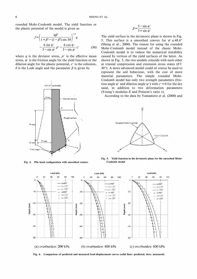
Fig. 6. Comparison of predicted and measured load-displacement curves (solid lines: predicted; dots: measured)

6 SHENG ET AL.

rounded Mohr-Coulomb model. The yield function orthe plastic potential of the model is given as

f＝Ø 4b4

1＋b4－(1－b4) sin 3u»1/4

q

－6 sin q?

3－sin q?p?－

6 cos q?

3－sin q?c? (36)

where q is the deviator stress, p? is the eŠective meanstress, q? is the friction angle for the yield function or thedilation angle for the plastic potential, c? is the cohesion,u is the Lode angle and the parameter b is given by

b＝3－sin q?

3＋sin q?

The yield surface in the deviatoric plane is shown in Fig.5. This surface is a smoothed convex for q?Ã48.69(Sheng et al., 2000). The reason for using the roundedMohr-Coulomb model instead of the classic Mohr-Coulomb model is to reduce the numerical instabilitycaused by vertices of the yield surfaces of the latter. Asshown in Fig. 5, the two models coincide with each otherat triaxial compression and extension stress states (u309). A more advanced model could of course be used torepresent the soil behaviour, with the cost of morematerial parameters. The simple rounded Mohr-Coulomb model has only two strength parameters (fric-tion angle q? and dilation angle c?) with c?＝0 for the drysand, in addition to two deformation parameters(Young's modulus E and Poisson's ratio n).

According to the data by Yamamoto et al. (2000) and

7

Fig. 7. Deformed mesh and stress contours (srr: radial stress; szz: vertical stress; srz: shear stress; suu: circumferential stress; cone angle 609; over-burden＝200 kPa)

7ENLARGED END PILES USING FRICTIONAL CONTACT

Li and Yamamoto (2005), the friction angle (at criticalstate) of the sand is 309, with a dilation angle of 159. ThePoisson ratio of the soil is assumed to be 0.333, whichcorresponds to a K0 value of 0.5. The Young modulus ofthe soil that best ˆts one of the experimental load-displacement curves is about 98 MPa (see discussionabout Fig. 6) and therefore a rounded-up value of 100MPa is used in all the analysis.

The steel pile is assumed to be elastic with a Young'smodulus of 200 GPa and Poisson's ratio of 0.3. The pilesurface is smoothed according to Fig. 4, with the smooth-ing parameter a setting to 1/6. The soil-pile interface isassumed to be smooth along the pile shaft (above point Ain Fig. 4), but rough along the pile end (below point A inFig. 4) with a soil-pile interfacial frictional angle of 309.

In the simulation, the penalty parameters for normal

and tangential contact are both set to 109 kN/m3, i.e.about 200 times of the soil stiŠness divided by the thick-ness of the soil elements close to the pile. Test runs indi-cate that this value can be reduced or increased by oneorder of magnitude, without causing much change of thenumerical results. The prescribed displacement at the pilehead, i.e. 50 mm penetration, is applied in 1000 equal in-crements. The Newton-Raphson scheme (Sheng et al.,2006) is used to solve the global equations within each in-crement. All the analyses are carried out using the ˆniteelement code SNAC, developed at the University of New-castle over the last 10 years or so.

NUMERICAL RESULTS AND DISCUSSION

In the tests carried out by Yamamoto et al. (2000), a

8

Fig. 7. Cont. Deformed mesh and stress contours (srr: radial stress; szz: vertical stress; srz: shear stress; suu: circumferential stress; cone angle 609;overburden＝200 kPa)

8 SHENG ET AL.

load transducer was placed in the pile head, with the pileshaft wrapped with thin layers of Te‰on sheets. The loadsmeasured at the transducer are then plotted against thesettlement of the pile. In the numerical simulation, thepile is pushed into the soil by prescribed displacements atthe pile head. The vertical reaction forces at the pile headare the summed up to the pile load. The pile loads socomputed are plotted against the pile penetration in Fig.6, where the measured pile loads are also shown. As men-tioned above, one soil parameter, Young's modulus E,was best ˆtted to match the experimental load-displace-ment for the pile with a cone angle of 1209and an over-burden pressure of 400 kPa. The best-ˆtted value (E＝97MPa) was then rounded up to 100 MPa and used in allthe other analyses. In general, the computed load-displacement curves are very close to the experimental

curves. The maximum discrepancy between the computedand measured loads is about 6.4z which occurs for thecase of the pile with a cone angle of 1809and the soil withan overburden of 600 kPa. A noticeable diŠerence be-tween the computed and measured load-displacementcurves is that the former seems to be less aŠected by thecone angle. The curves for the pile with a cone angle of1209were best predicted by the numerical model (Fig.6(a)–(c)). The predicted loads for the pile with a cone an-gle of 609are generally larger than the correspondingmeasured values (Fig. 6(a), 6(c)), whereas the loads forthe pile with a cone angle of 1809are smaller than themeasured values (Fig. 6(a), 6(c)).

Figure 7 shows the deformed meshes and stress con-tours for the pile with a cone angle of 609and the over-burden pressure of 200 kPa. For each stress component,

9

Fig. 8. Plastic strain contours (eprr: plastic radial strain; ep

zz: plastic vertical strain; epuu: plastic circumferential strain; ep

rz: shear strain; cone angle1209; overburden＝200 kPa)

9ENLARGED END PILES USING FRICTIONAL CONTACT

the contours are plotted at three speciˆc penetrationdepths. We ˆrst notice that the pile was successfullypushed into soil and large relative sliding occurs along thepile-soil interface, particularly along the pile shaft wherethe interface is frictionless. Along the upper part of thepile end (part AB in Fig. 4), the soil seems to move down-wards together with the pile and no large cavity is left be-hind the pile. This pattern of deformation is caused by

the friction of the interface and the vertical compressivepressure applied at the soil surface. Along the pile surfaceBCDE, some relative sliding between the soil and the pileoccurs, which has caused some slight distortion of a fewsoil elements just below the pile end (Fig. 7(c)). In gener-al, the deformed meshes show a reasonable deformationpattern of the soil as the pile is pushed in.

The contours of radial stress (srr) in Fig. 7(a)–(c) show

10

Fig. 9. Active plastic zones (cone angle 1209; overburden＝200 kPa)

10 SHENG ET AL.

that this stress has increased from an initial homogeneousvalue of －100 kPa to somewhere between 4000–10000kPa in the elements just beneath the pile end. The com-pressive stress is taken as positive in all the stress con-tours. The stress bulb under the pile end increases as thepile penetrates, as expected. In the pile, the highest radialstress occurs at the pile shaft and is around 20000 kPa.The lowest srr in the pile occurs at the pile conical tip andis around 7500 kPa. No tensile radial stresses are ob-served in the pile.

The contours of the vertical stress (szz) are shown inFig. 7(d)–(f). The maximum compressive stresses in thesoil occur in the elements just below the pile end. At thepenetration depth of 45 mm, the maximum vertical stressin the soil is around －10000 kPa. The vertical stresses inthe pile vary between 10000–40000 kPa, with the highestvertical stress in the pile shaft (around 40000 kPa) and thelowest in the pile end (around 10000 kPa).

The circumferential (hoop) stress (suu) distributions inthe soil and the pile show similar patterns as the radialstress distributions. This stress varies between 3500–7000in the soil elements just beneath the pile end (Fig.7(g)–(i)), less signiˆcant compared to srr and szz. In thepile, the maximum circumferential stress is around 18000kPa in the pile shaft and the minimum 5000 kPa in thepile end. The maximum shear stress (srz) in the soil isaround 4000 kPa, in the soil elements beneath the pileend (Fig. 7(j)–(l)). The maximum shear stress in the pile isaround 5000 kPa, near point A where the pile surfacechanges from smooth to frictional.

The contours of plastic strains at the penetration depthof 45 mm are shown in Fig. 8. Again, compressive strainsare taken as positive. The plastic radial strain in the soilnear the pile changes from tension near the pile tip (pointE), to compression near points D, C and B, and to a ten-sion again near point A. The plastic vertical strain in the

soil changes from compression beneath the pile tip to ten-sion along the side CBA. The hoop strain is in tension inthe soil beneath the pile end, but in compression aroundpoint A. The active plastic zones are shown in Fig. 9. Theactive plastic zone initially expands until it reaches the topand bottom boundaries (Fig. 9(a)–(b)), and is then deac-tivated from above and below due to the boundary con-straints (Fig. 9(c)).

The stress and strain contours for the pile with a coneangle of 1209are plotted over the deformed meshes atpenetration depth of 21 mm in Fig. 10. We see that thesoil elements beneath the pile end and around the pileshoulder are more distorted than the case for the pile witha cone angle of 609. Again, large relative sliding occursalong the pile shaft and along the surface BA. However,very little relative sliding occurs along the pile end (thesegment CDE in Fig. 4). The maximum radial, verticaland circumferential stresses in the soil again occur in theelements just beneath the pile conical end. The maximumradial, vertical and circumferential stresses in the pileagain occurs in the pile shaft. The radial stress in the piletip (point E) smaller than those at points D and C. Theplastic radial strain ep

rr in the soil changes from tensionbeneath the pile end (near point D), to compression nearpoint B and then to tension near point A. The plastic ver-tical strain ep

zz changes from compression beneath the pileend EDC) to tension above the pile shoulder (CBA). Theplastic circumferential strain changes from tension belowEDC to compression along BA.

For the pile with a cone angle of 1809, the deformedmeshes shown in Fig. 11 are also distorted, particularlyfor the elements near the corner of the pile ends. Thismesh distortion is due to the Updated Lagrangianmethod used in the analysis. It may even cause somesmall negative radial displacements at the axis of symmet-ry. To overcome such mesh distortion, more advanced

11

Fig. 10. Deformed mesh and stress and strain contours (srr: radial stress; szz: vertical stress; suu: circumferential stress; radial plastic strain; epzz: ver-

tical plastic strain; epuu : circumferential strain; cone angle 1209; overburden＝200 kPa)

11ENLARGED END PILES USING FRICTIONAL CONTACT

methods, such as the Arbitrary Lagrangian-Eulerianmethod (Nazem et al., 2006), may have to be used.Figures 11 also show some element overlapping near thecorner of the pile end (position C in Fig. 4). This overlap-ping is partly due to the relatively coarse linear elementsused, and partly due to the smoothing of the pile surfacearound the corner. In theory the mesh should be kept asˆne as possible, particularly around the pile where strainis large. However, a very ˆne mesh may not be able toproduce a numerical solution, due to possibly severemesh distorion.

The maximum values of srr, szz and suu in the soil inFig. 11 are higher than those observed for the piles with acone angle of 609or 1209. The stress distributions in thesoil are of similar patterns as those with a cone angle of

609and 1209. As for the pile with a conical end of 1209,the radial stress in the pile centre (point E) is lower thanthose near the edge of then end (point C), indicating thepotential of tensile cracking at the centre. Indeed, theradial stress at point E can evolve to a negative value.This tensile radial stress is not shown in Fig. 11(a) due tothe low resolution of the stress contours. The results con-ˆrm the experimental observation that a concrete or ce-ment pile with a ‰at end may develop tensile cracks at itscentre, which is the exact reason that a conical end is usu-ally used instead. The plastic strain contours in Fig.11(d)–(f) show similar patterns as those in Fig. 8 and Fig.10.

Figure 12 shows the deformed mesh and the zoom-upof pile-soil surface for the pile with a cone angle of 609.

12

Fig. 11. Deformed mesh and stress contours (srr: radial stress; szz: vertical stress; srz: shear stress; suu: circumferential stress; cone angle 1809;overburden＝200 kPa)

12 SHENG ET AL.

In this ˆgure, large relative sliding along the pile-soil in-terface can be noticed. The magniˆed part of the meshclearly shows the surface separation and re-closure be-tween the soil and the pile (Fig. 12(b)). Such an interfa-cial behaviour can not be modelled with interface or jointelements.

Another note that should be made here is the possibleparticle crushing caused by the high stresses generatedbeneath the pile end. The maximum mean stresses in thesoil are in the order of 10000 kPa, which is su‹cient tocause particle crushing of the sand. To take into accountthe crushing phenomenon, we will have to use more ad-vanced soil models that will eventually need more materi-al parameters. Such elaboration should in theory lead tomore reliable results if the material parameters could beestimated with conˆdence. On the other hand, we have in

this paper used a simple soil model and back-estimatedone key material parameter and have achieved satisfacto-ry results. The back-estimated parameter (in this case theYoung modulus of the soil) may not represent the truevalue of the soil, but re‰ects the combined eŠects of theother facts such as particle crushing. Such a simpliˆed ap-proach can of course be very useful if we can carry outthe back-estimation with conˆdence.

CONCLUSIONS

This paper presents a modiˆed formulation of frictioncontact for the soil-pile interaction. The modiˆed formu-lation is based on the smooth discretisation of the pilesurface using the B ÁEZIER polynomials. The ˆnite elementmodel based on this new formulation is then used to ana-

13

Fig. 12. Zoom-up of the deformed mesh, showing pile-soil separation (penetration depth: 45 mm)

13ENLARGED END PILES USING FRICTIONAL CONTACT

lyse pile loading tests in Toyoura sand. The steel pileshave enlarged ends with diŠerent shapes and are modelledas an elastic material. The Toyoura sand is modelled by arounded Mohr-Coulomb model. It is demonstrated that,even with the simpliˆed approach to model the soil andpile behaviour, the new ˆnite element formulation is ableto produce reasonable results for the pile loading prob-lem. Such a problem involves large interfacial sliding andsurface separation and would be very di‹cult to solveotherwise.

The numerical analysis presented in this paper can beimproved in a number of aspects. For example, more ad-vanced numerical algorithms can be used to tackle themesh distortion problem associated with large deforma-tion. The constitutive model used for the soil is too sim-plistic and more advanced models, particularly those withthe capability to model particle crushing, can be incorpo-rated into the analysis. In addition, the soil analysed inthis study is assumed to be completely dry. In the future,coupled analysis that takes into account both deforma-tion and pore pressure generation/dissipation can be de-veloped and applied. Formulation incorporating impactelements can also be developed to tackle dynamic loadingof piles.

ACKNOWLEDGEMENT

The research carried out in this paper is sponsored bythe Australian Research Council (ARC) DiscoveryProject (DP0557161), which also includes a visiting grantto support the visit of the second author (H. Yamamoto)

to the University of Newcastle during October andNovember of 2005. This ˆnancial support from ARC isappreciated.

REFERENCES

1) Li, W., Ikeda, K., Yamamoto, H. and Tominga, K. (2003): Meas-urement of soil displacement around pile tip by digital image analy-sis, Geotechnical Engineering in Urban Construction (eds. by Yu,Y. and Akagi, H.), Tsinghua University Press, Beijing, China,393–400.

2) Li, W. and Yamamoto, H. (2005): Numerical analysis on soil be-haviour around pile-tip under vertical load, Journal of Structuraland Construction Engineering (Transaction of AIJ), 51B, 147–157.

3) Nazem, M., Sheng, D. and Carter, J. P. (2006): Stress integrationand meshing reˆnement for large deformation in geomechanics, In-ternational Journal for Numerical Methods in Engineering, 65,1002–1027.

4) Sheng, D., Axelsson, K. and Magnusson, O. (1997): Stress andstrain ˆelds around a penetrating cone, Numerical Models in Geo-mechanics (eds. by Pietruszczak, S. and Pande, G. N.), Balkema,Rotterdam, 653–660.

5) Sheng, D., Sloan, S. W. and Yu, H. S. (2000): Aspects of ˆnite ele-ment implementation of critical state models, ComputationalMechanics, 26, 185–196.

6) Sheng, D. and Sloan, S. W. (2001): Load stepping methods for crit-ical state models, International Journal for Numerical Methods inEngineering, 50, 67–93.

7) Sheng, D., Eigenbrod, K. D. and Wriggers, P. (2005): Finite ele-ment analysis of pile installation using large-slip frictional contact,Computers and Geotechnics, 32(1), 17–26.

8) Sheng, D., Sun, D. A. and Matsuoka (2006): Cantilever sheet-pilewall modelled by frictional contact, Soils and Foundations, 46(1),29–37.

9) Simo, J. C. and Meschke, G. (1993): A new class of algorithms for

1414 SHENG ET AL.

classical plasticity extended to ˆnite strains. Application to ge-omaterials, Computational Mechanics, 11(4), 253–278.

10) Wriggers, P. (2002): Computational Contact Mechanics, JohnWiley & Sons, Chichester.

11) Yamamoto, H., Xu, T. and Tominaga, K. (2000): EŠects of over-burdening pressures and end shapes on bearing capacities of under-reamed end piles, Developments in Geotechnical Engineering (eds.by Balasubramaniam, A. S. et al.), Asian Institute of Technology,Bangkok, Thailand, 255–261.

APPENDIX: B ÁEZIER INTERPOLATIONFUNCTIONS

The standard B ÁEZIER polynomials are given as follows

B1(j )＝18

(1－j )3

B2(j )＝38

(1－j )2(1＋j )

B3(j )＝38

(1－j )(1＋j )2

B4(j )＝18

(1＋j )3 (A1)

When we use the special interpolation deˆned in Fig. 1,the B ÁEZIER interpolation is based on three nodes with theinterpolation functions

B̃1(j )＝12

[B1(j )＋(1－a)B2(j )]

B̃2(j )＝12

[B1(j )＋(1＋a)(B2(j )＋B3(j ))＋B4(j )]

B̃3(j )＝12

[B4(j )＋(1－a)B3(j )] (A2)

Further functions used in the stiŠness matrices:

BN(j̃ )＝

šn－B̃1(j̃ ) šn－B̃2(j̃ ) šn－B̃3(j̃ ) šn

(A3)

BN, j(j̃ )＝

0B̃1, j(j̃ ) šnB̃2, j(j̃ ) šnB̃3, j(j̃ ) šn

(A4)

BT(j̃ )＝

šxs, j

－B̃1(j̃ ) šxs, j

－B̃2(j̃ ) šxs, j

－B̃3(j̃ ) šxs, j

(A5)

Bj(j̃ )＝H－1jj [BT(j̃ )＋gNsBN, j(j̃ )] (A6)

H－1jj ＝( ša11－gNs šn1･ šx1

, jj)－1 (A7)

ša11＝ šx1, j(j̃)･ šx1

, j(j̃) (A8)

b̃1jj＝ šx1

, jj･ šn1 (A9)