Computers and Structures 88 (2010) 1239–1247

Contents lists available at ScienceDirect

Computers and Structures

journal homepage: www.elsevier .com/locate /compstruc

Finite element analysis of laterally loaded fin piles

J.-R. Peng, M. Rouainia *, B.G. ClarkeSchool of Civil Engineering and Geosciences, Newcastle University, Newcastle upon Tyne, NE1 7RU, UK

a r t i c l e i n f o

Article history:Received 13 August 2009Accepted 5 July 2010Available online 23 August 2010

Keywords:Fin pilesMonopilesMohr–Coulomb soil model3D finite element modelsCapacity of laterally loaded pilesEfficiency of fins

0045-7949/$ - see front matter � 2010 Elsevier Ltd. Adoi:10.1016/j.compstruc.2010.07.002

* Corresponding author. Tel.: +44 191 222 3608; faE-mail address: M.Rouainia@ncl.ac.uk (M. Rouaini

a b s t r a c t

A three-dimensional analysis of laterally loaded fin piles is presented. The behaviour of fin piles is diffi-cult to explain using simple pile–soil theories or two dimensional numerical analyses because of the com-plicated geometry of the piles. In this study, a nonlinear 3D analysis with an elastic plastic soil model, anelastic pile material and interface elements are used to model the pile–soil interaction. Experimental dataconfirmed that the predicted behaviour of a monopile was acceptable leading to a more detailed study ofthe impact of fins upon the lateral resistance. The stress distribution within the pile and the deformationof the fin pile are presented. The increase in resistance gained by placing fins on a pile is illustrated byplotting the lateral resistance against displacement of the pile head for various geometries of the pile.This is expressed as the efficiency of the fins which is the ratio of the lateral resistance of a fin pile to thatof a monopile with the same core diameter where the lateral resistance is defined as the resistance at adisplacement of 10% of the pile diameter. The efficiency of the piles increases as the length of the fins; theincrease is independent of the loading direction relative to the fins.

� 2010 Elsevier Ltd. All rights reserved.

1. Introduction

The challenges of tackling climate change and ensuring thesecurity of energy supply has led the world in a quest to developalternative sources of renewable energy. There are various sourcesof renewable energy, such as tidal, wave, solar, but one of the mostpromising sources is wind energy. The fastest growing sector inwind energy has been onshore wind farms but there is now anincreasing demand for offshore wind farms because they offer anumber of advantages over onshore wind farms. The constructionof offshore wind farms is more challenging than onshore windfarms because of the environment which creates a different con-struction regime and a different set of loading conditions. Onshorepiles are usually used to transmit large vertical loads from thesuperstructure through weaker subsoil into the underlying bearingstrata. Horizontal loads acting on pile foundations are often ig-nored as, in many cases; they are much smaller than the verticalloads. Foundations for offshore structures, however, withstand sig-nificant environmental loads from waves, currents and wind givingrise to lateral loads that could be up to one third of the verticalloads [10]. The significant increase in offshore wind farms hasled to the use of large diameter monopiles to resist both gravityloads and significant environmental loads transmitted from thesuperstructure. For example, a 3 MW wind turbine which has aweight of over 154T in 25 m of water will be supported by a pilewith a diameter of 6 m and an embedded length of 20 m [3]. Allen

ll rights reserved.

x: +44 191 222 3522.a).

[1] suggested that the cost of manufacture, transport and installa-tion could be reduced by using fins to enhance the lateral resis-tance of the upper layers of soil rather than rely on transmittingthe lateral load to depth. Peng et al. [7] showed from a series of1G model tests that this was the case. Many FDM and FEM com-puter codes such as LPILE, SWM, FLAC, PLAXIS and ABAQUS havebeen successfully used in the study of laterally loaded circular piles[2,4,6,9,11,12]. Developments in interface elements, constitutivemodels for soils including nonlinearity, and developments in pilegeometries and loading conditions now enable real environmentalconditions and non-standard pile geometries to be modelled moreaccurately. This paper presents 3D computer simulations of later-ally loaded fin piles to explore the effect of fin dimensions on theirload bearing capacity in sand. It should be noted that the numericalanalyses were carried out using the standard Mohr–Coulomb mod-el in order to assess the potential of fin piles to reduce foundationcosts.

2. Methodology

2.1. Material properties

The sand was assumed to be a linear elastic perfectly plasticmaterial. A non-associated Mohr–Coulomb constitutive modelwas assumed to govern the soil behaviour for which the materialparameters are well established in geotechnical engineering prac-tice. The yield function, f , and the plastic potential, g, are given bythe following equations in terms of invariants:

1240 J.-R. Peng et al. / Computers and Structures 88 (2010) 1239–1247

f ¼ p0 sin u0 þffiffiffiffiJ2

pcos h�

ffiffiffiffiJ2

3

rsin u sin h� c0 cos u0 ð1Þ

g ¼ p0 sin wþffiffiffiffiJ2

pcos h�

ffiffiffiffiJ2

3

rsin w sin h ð2Þ

where /0 the effective friction angle, w is the dilatancy angle and c0

is the effective cohesion. In the above expressions J2 ¼ 12 SijSij is the

second invariant of the deviator stress withsij ¼ rij � p0dij; p0 ¼ 1

3 rii is the mean pressure and h is the Lode’s an-gle given by

h ¼ 13

sin�1 �3ffiffiffi3p

2J2

J3=23

!with J3 ¼

SijSjkSkiij

3ð3Þ

where J3 is the third invariant of deviator stress.

Fig. 1. A schematic diagram of a fin pile.

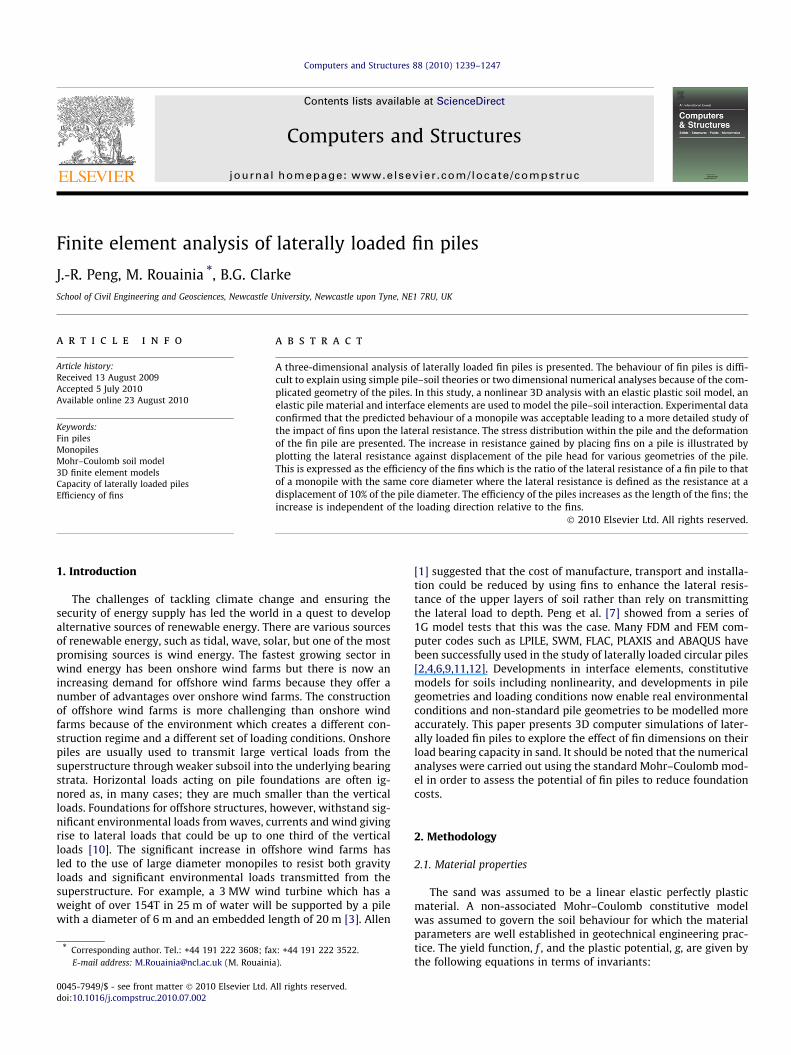
Fig. 2. The finite element used to model the laterally loaded pile and sand showing (a) thpile); and (b) 3D view of the fin pile. (For interpretation of the references in colour in th

An elasto-plastic analysis under drained conditions was used tomodel the full scale and laboratory scale piles with the yield of thesand, defined by the Mohr–Coulomb model, being the upper limitto the elastic behaviour of the sand. In the full scale analysis, theelastic soil properties, corresponding to medium dense sand, wereassumed to be: Poisson’s ratio ts = 0.33, and dry unit weightcs = 16.5 kN/m3. The Mohr–Coulomb model had an effective fric-tion angle /0 = 35o, dilatancy angle w = 0� and effective cohesivestrength c0 = 0 kPa. In order to account for the variation in soilproperties with depth, Young’s modulus was assumed to increaselinearly according to:

ESðZÞ ¼ ES0 þ Esin cðz� z0Þ ð4Þ

where ES0 is Young’s modulus at the soil at depth z0 and Esinc is theincrease of Young’s modulus per unit of depth. For the full scalesimulations, it was assumed that ES0 = 10 MPa at the surface and arate of increase Esinc = 1 MPa/m. The two values are chosen to givea value of 30 MPa [5] at a depth of 20 m. It was assumed that thepile was installed in a normally consolidated sand with Ko = 0.42.It should be noted that interface elements were applied betweenthe soil and the pile in order to model the soil–pile interaction.Along the pile the strength reduction factor of the interface (Rinter)is set to 0.65 which is typical of sand steel interfaces. This factor re-lates the interface properties to the strength properties of a soillayer as follows:

tan ui ¼ Rint tan u0 ð5ÞCi ¼ Rintc0

wi ¼ 0 if Rint < 1 otherwise wi ¼ w

where /i, ci and w are the friction angle, cohesion and dilatancy an-gle of the interface, respectively. The piles and the fins, shown inFig. 1, were assumed to be linear elastic mild steel material whichhas typical properties of Young’s modulus, Ep = 200 GPa, Poisson’sratio, tp = 0.3, and unit weight, cp = 78 kN/m3. The yield of steelwas not considered in this study. The same parameters were usedfor modelling the laboratory scale piles as those used for the fullscale piles with the exception of the modulus of elasticity of thesand, ES. The stiffness of the sand used in the laboratory tests wasmeasured directly with a volume displacement pressuremeter de-signed and built to determine the in situ stiffness of the laboratory

e full a three-dimensional mesh (the red arrow show the loading direction of the finis figure legend, the reader is referred to the web version of this article.)

J.-R. Peng et al. / Computers and Structures 88 (2010) 1239–1247 1241

soil [8]. The pressuremeter was embedded in the sand prior to car-rying out an expansion test at a constant rate of increase of pres-sure. The analysis of the resulting applied pressure cavity straincurve gave an average ES of about 1200 kPa. For the laboratory scalesimulations, Young’s modulus was also assumed to increase linearlywith depth with ES0 = 0.75 MPa at the surface and a rate of increaseEsinc = 0.4 kN/m2/mm. The two values are chosen to give a correctvalue of ES = 1200 kPa at a depth of 0.5 m.

2.2. The 3D geometry of the embedded pile and the 3D soil mesh

The three-dimensional finite element program, PLAXIS-3D waschosen to model the pile and the sand. The boundary is a cube withsides of 22.5 times the diameter of the pile and a depth 2.5 timesthe pile length. The geometry of a three-dimensional model of apile embedded in soil is shown in Fig. 2. The bottom boundarywas fixed against movements in all directions, whereas the ‘ground

Table 1Properties of the piles.

Parameter Model pile Full scale pile

Material Steel SteelModulus of elasticity 200 GPa 200 GPaLength 400 mm 40 mOuter diameter 44.5 mm 4 mWall thickness 2.1 mm 50 mmFin wall thickness 2.9 mm 50 mm

Table 2Geometry of the piles.

Pile code Fin length Fin width Moment of inertia Cross sectional area

MPS 0 mm 0 mm 64262 mm4 286 mm2

FPS210 100 mm 20 mm 210658 mm4 541 mm2

FPS220 200 mm 20 mm 210658 mm4 541 mm2

FPS240 400 mm 20 mm 210658 mm4 541 mm2

MPF 0 m 0 m 1.21 m4 0.62 m2

FPF210 10 m 2 m 3.08 m4 1.02 m2

FPF220 20 m 2 m 3.08 m4 1.02 m2

FPF240 40 m 2 m 3.08 m4 1.02 m2

The moment of inertia (calculated in line with the fins) and cross sectional area(calculated in line with the fins) are based on the section including the fins

Table 3The specifications of the models used in the finite element analyses.

Pile code Pilecharacteristics

Loadingdirection

Interfacecoefficient

Wallthickness(m)

Scale

MPF normala 0.65 0.05 FullFPF210 Normal Fins in line 0.65 0.05 FullFPF220 Normal Fins in line 0.65 0.05 FullFPF240 Normal Fins in line 0.65 0.05 FullMPS Normal Fins in line 0.65 0.002 SmallFPS210 Normal Fins in line 0.65 0.002 SmallFPS220 Normal Fins in line 0.65 0.002 SmallFPS240 Normal Fins in line 0.65 0.002 SmallFPS210_45 Normal 45o to fins 0.65 0.002 SmallFPS210_22 Normalb Fine in line 0.65 0.002 SmallFPS210_M Fins in middle Fins in line 0.65 0.002 SmallFPS210_B Fins at base Fins in line 0.65 0.002 SmallFPS210_L1 Lp = 375 mm Fins in line 0.65 0.002 SmallFPS210_L2 Lp = 350 mm Fins in line 0.65 0.002 SmallMPS_6 Dp = 66 mm Fins in line 0.65 0.002 SmallMPS_8 Dp = 89 mm Fins in line 0.65 0.002 Small

a Core diameter 4 m for full scale piles; 40 mm for laboratory scale piles.b 22 mm wide fins.

surface’ was free to move in all directions. The vertical boundarieswere fixed against movements in the direction normal to them.This geometry approximated that used by Peng et al. [7] in their1G laboratory tests on model piles. The model piles were 1/100ththe size of a typical monopile, that is 44.5 mm in diameter withan embedded length of 400 mm (see Table 1). The tank was990 mm wide creating a ratio of pile diameter to tank width of1:20. The bottom of the 400 m long model pile was 600 mm abovethe base of the tank. Results of the laboratory tests showed thatthere was little or no movement of the pile base. The pile wasset in the middle of the cube of soil, with the pile flush with thetop of the cube. The mesh was automatically generated from thesoftware package and consisted of �3000 elements and �9000nodes. The soil mesh was based on 15-node wedge elements whichare generated from 6-node triangular elements. Shell elementswere used to model the thin walled pile, the fins and pile/sandinterface.

2.3. The pile dimensions

The dimensions of the piles used in the laboratory tests and thenumerical analyses are given in Tables 2 and 3. The piles were ana-lysed to allow comparisons to be made with the results of the lab-

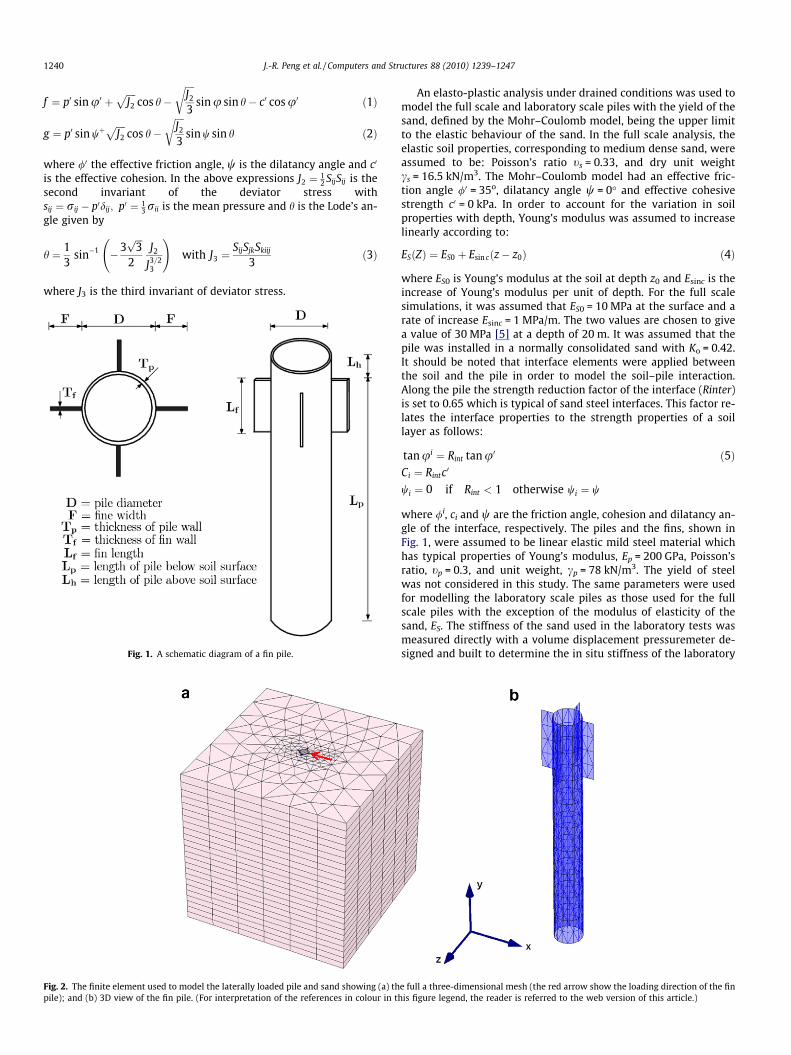
Fig. 3. The pile head displacement curves (P–Y curves) from the analyses of (a) thefull scale piles and (b) the model piles.

1242 J.-R. Peng et al. / Computers and Structures 88 (2010) 1239–1247

oratory tests on the model piles and to make predictions of the fullscale pile behaviour. The laboratory monopile (MPS) was a hollowcircular steel pile with a diameter of 44.5 mm, an embedded lengthof 0.4 m and a wall thickness of 2.1 mm. The laboratory fin piles

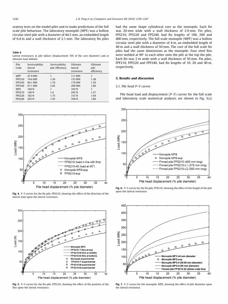
Table 4Lateral resistances at pile failure (displacement 10% of the core diameter) and atultimate load defined.

PileCode

Serviceabilitylateralresistance

Serviceabilitypile efficiency

Ultimatelateralresistance

Ultimatepileefficiency

MPF 47.9 MN 1 111 MN 1FPF210 74.6 MN 1.56 153 MN 1.38FPF220 84.1 MN 1.76 176 MN 1.59FPF240 97.1 MN 2.02 209 MN 1.89MPS 104 N 1 192 N 1FPS210 146 N 1.4 245 N 1.27FPS220 182 N 1.75 315 N 1.64FPS240 203 N 1.95 358 N 1.86

Fig. 4. P–Y curves for the fin pile, FPS210, showing the effect of the direction of thelateral load upon the lateral resistance.

Fig. 5. P–Y curves for the fin pile, FPS210, showing the effect of the position of thefins upon the lateral resistance.

had the same shape cylindrical core as the monopile. Each finwas 20 mm wide with a wall thickness of 2.9 mm. Fin piles,FPS210, FPS220 and FPS240, had fin lengths of 100, 200 and400 mm, respectively. The full scale monopile (MPF) was a hollowcircular steel pile with a diameter of 4 m, an embedded length of40 m and a wall thickness of 50 mm. The core of the full scale finpiles had the same dimensions as the monopile. Four steel finswere welded at 90� to each other onto the pile at the top the pile.Each fin was 2 m wide with a wall thickness of 50 mm. Fin piles,FPF210, FPF220 and FPF240, had fin lengths of 10, 20 and 40 m,respectively.

3. Results and discussion

3.1. Pile head P–Y curves

Pile head load and displacement (P–Y) curves for the full scaleand laboratory scale numerical analyses are shown in Fig. 3(a)

Fig. 6. P–Y curves for the fin pile, FPS210, showing the effect of the length of the pileupon the lateral resistance.

Fig. 7. P–Y curves for the monopile, MPS, showing the effect of pile diameter uponthe lateral resistance.

J.-R. Peng et al. / Computers and Structures 88 (2010) 1239–1247 1243

and (b), respectively. The ultimate load was taken at the pointwhere the P–Y curve tends to a straight line which is defined as achange in slope of less than 0.05 MN/m; the pile failure load wastaken as a displacement of 10% of the pile diameter. Movementsof this magnitude could damage the structure; hence the use ofdisplacement to define failure. Table 4 shows lateral loads at theultimate load and at the pile failure state for each pile. The increasein resistances, expressed as pile efficiency of the fin piles expressedas a ratio of the resistance of the monopile at both the pile failureand ultimate conditions are also presented in Table 4. It shows thatthe percentage increase in lateral capacity at pile failure exceedsthat for the ultimate load for a given fin dimension; that is the effi-ciency of the piles is greater at lower loads. The efficiency of thesmall, laboratory scale piles is less than that of the full scale modelthough, as with the full scale piles, the efficiency is greater at lowerloads. Such a difference in efficiency between the full scale and lab-oratory scale piles could arise from the use of different ratios of pileto soil stiffness and is not necessarily a function of the size of pile.

The numerical analyses on laboratory scale piles were carriedout to compare the results with those from laboratory tests [8]to demonstrate that the analyses gave acceptable results. The pilehead P–Y curves generated from the numerical analyses of a finnedpile using PLAXIS-3D have been compared with that of a model testshowing that the numerical method can be used to predict pileperformance though the accuracy could be improved at displace-ments exceeding 10% of the pile diameter for the fin pile FPS220.It can be seen from Fig. 3(b) that when the lateral displacementat the top of the pile is 10% of the core diameter, the predicted loadfrom the model test are 112, 140 and 170 N for MPS, FPS210 andFPS220, respectively, are similar to that predicted by the numericalanalyses. In practice the pile is not going to move more than 10% ofits diameter which suggests that the numerical analysis is anacceptable model of the pile behaviour.

One issue that has to be considered is the direction of the envi-ronmental loads in relation to the direction of the fins. Fig. 4 showsthat, for the laboratory scale fin pile, FPS210, the P–Y curves whenthe load is applied at 45� to the fins is in excess of that when theload is applied at 0� to the major fin axis. However, they are bothin excess of the monopile by at least 30%. The increase in load car-rying capacity at 45� is possibly due to the increased moment of

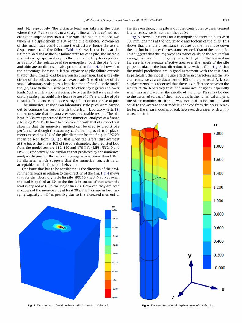
Fig. 8. The contours of total horizontal displacements of the soil.

inertia even though the pile width that contributes to the increasedlateral resistance is less than that at 0�.

Fig. 5 shows P–Y curves for a monopile and three fin piles with100 mm long fins at the top, middle and bottom of the piles. Thisshows that the lateral resistance reduces as the fins move downthe pile but in all cases the resistance exceeds that of the monopile.This suggests that the improved resistance could be the result of anaverage increase in pile rigidity over the length of the fins and anincrease in the average effective area over the length of the pileperpendicular to the load direction. It is evident from Fig. 5 thatthe model predictions are in good agreement with the test data.In particular, the model is quite effective in characterising the lat-eral resistance at a displacement of 10% of the pile head. At largerdisplacements, it is observed that there is a difference between theresults of the laboratory tests and numerical analyses, especiallywhen fins are placed at the middle of the piles. This may be dueto the assumed values of shear modulus. In the numerical analysis,the shear modulus of the soil was assumed to be constant andequal to the average shear modulus derived from the pressureme-ter test; the shear modulus of soil, however, decreases with an in-crease in strain.

Fig. 9. The contours of total displacements of the fin pile.

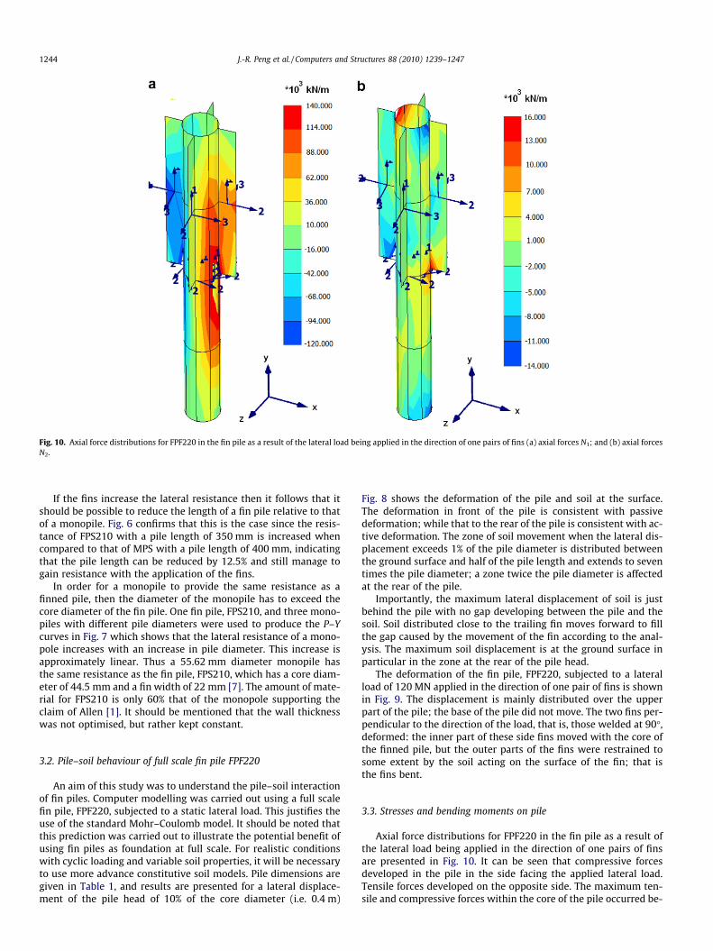
Fig. 10. Axial force distributions for FPF220 in the fin pile as a result of the lateral load being applied in the direction of one pairs of fins (a) axial forces N1; and (b) axial forcesN2.

1244 J.-R. Peng et al. / Computers and Structures 88 (2010) 1239–1247

If the fins increase the lateral resistance then it follows that itshould be possible to reduce the length of a fin pile relative to thatof a monopile. Fig. 6 confirms that this is the case since the resis-tance of FPS210 with a pile length of 350 mm is increased whencompared to that of MPS with a pile length of 400 mm, indicatingthat the pile length can be reduced by 12.5% and still manage togain resistance with the application of the fins.

In order for a monopile to provide the same resistance as afinned pile, then the diameter of the monopile has to exceed thecore diameter of the fin pile. One fin pile, FPS210, and three mono-piles with different pile diameters were used to produce the P–Ycurves in Fig. 7 which shows that the lateral resistance of a mono-pole increases with an increase in pile diameter. This increase isapproximately linear. Thus a 55.62 mm diameter monopile hasthe same resistance as the fin pile, FPS210, which has a core diam-eter of 44.5 mm and a fin width of 22 mm [7]. The amount of mate-rial for FPS210 is only 60% that of the monopole supporting theclaim of Allen [1]. It should be mentioned that the wall thicknesswas not optimised, but rather kept constant.

3.2. Pile–soil behaviour of full scale fin pile FPF220

An aim of this study was to understand the pile–soil interactionof fin piles. Computer modelling was carried out using a full scalefin pile, FPF220, subjected to a static lateral load. This justifies theuse of the standard Mohr–Coulomb model. It should be noted thatthis prediction was carried out to illustrate the potential benefit ofusing fin piles as foundation at full scale. For realistic conditionswith cyclic loading and variable soil properties, it will be necessaryto use more advance constitutive soil models. Pile dimensions aregiven in Table 1, and results are presented for a lateral displace-ment of the pile head of 10% of the core diameter (i.e. 0.4 m)

Fig. 8 shows the deformation of the pile and soil at the surface.The deformation in front of the pile is consistent with passivedeformation; while that to the rear of the pile is consistent with ac-tive deformation. The zone of soil movement when the lateral dis-placement exceeds 1% of the pile diameter is distributed betweenthe ground surface and half of the pile length and extends to seventimes the pile diameter; a zone twice the pile diameter is affectedat the rear of the pile.

Importantly, the maximum lateral displacement of soil is justbehind the pile with no gap developing between the pile and thesoil. Soil distributed close to the trailing fin moves forward to fillthe gap caused by the movement of the fin according to the anal-ysis. The maximum soil displacement is at the ground surface inparticular in the zone at the rear of the pile head.

The deformation of the fin pile, FPF220, subjected to a lateralload of 120 MN applied in the direction of one pair of fins is shownin Fig. 9. The displacement is mainly distributed over the upperpart of the pile; the base of the pile did not move. The two fins per-pendicular to the direction of the load, that is, those welded at 90�,deformed: the inner part of these side fins moved with the core ofthe finned pile, but the outer parts of the fins were restrained tosome extent by the soil acting on the surface of the fin; that isthe fins bent.

3.3. Stresses and bending moments on pile

Axial force distributions for FPF220 in the fin pile as a result ofthe lateral load being applied in the direction of one pairs of finsare presented in Fig. 10. It can be seen that compressive forcesdeveloped in the pile in the side facing the applied lateral load.Tensile forces developed on the opposite side. The maximum ten-sile and compressive forces within the core of the pile occurred be-

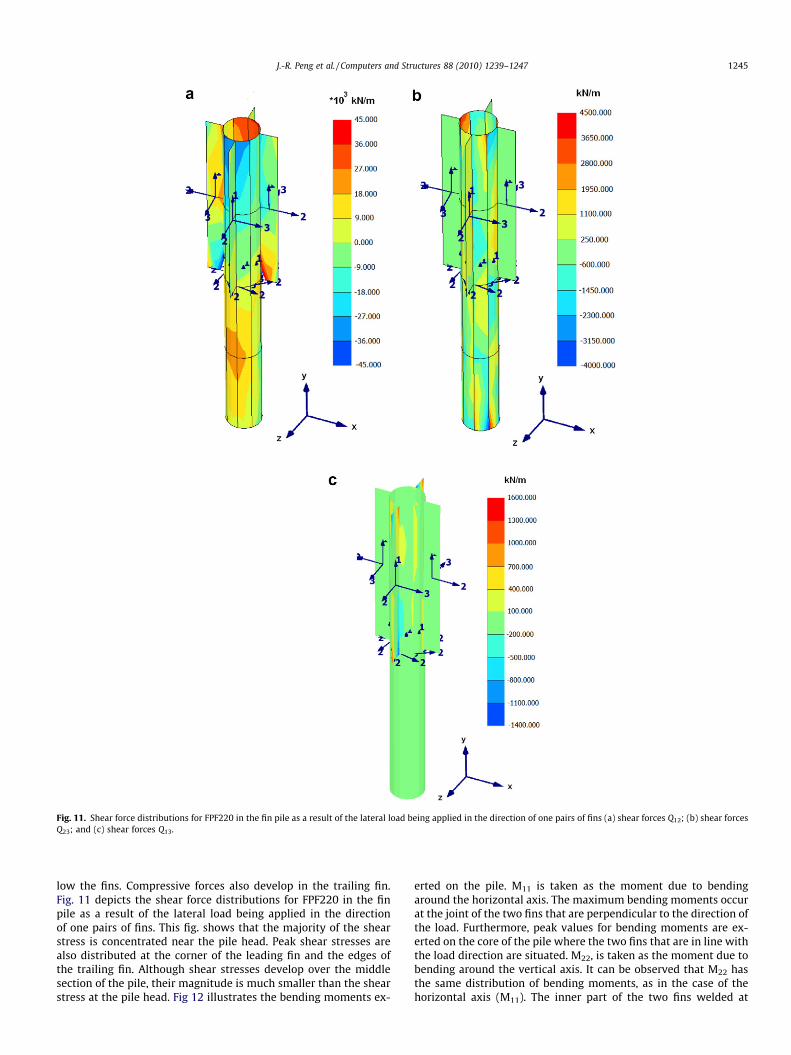
Fig. 11. Shear force distributions for FPF220 in the fin pile as a result of the lateral load being applied in the direction of one pairs of fins (a) shear forces Q12; (b) shear forcesQ23; and (c) shear forces Q13.

J.-R. Peng et al. / Computers and Structures 88 (2010) 1239–1247 1245

low the fins. Compressive forces also develop in the trailing fin.Fig. 11 depicts the shear force distributions for FPF220 in the finpile as a result of the lateral load being applied in the directionof one pairs of fins. This fig. shows that the majority of the shearstress is concentrated near the pile head. Peak shear stresses arealso distributed at the corner of the leading fin and the edges ofthe trailing fin. Although shear stresses develop over the middlesection of the pile, their magnitude is much smaller than the shearstress at the pile head. Fig 12 illustrates the bending moments ex-

erted on the pile. M11 is taken as the moment due to bendingaround the horizontal axis. The maximum bending moments occurat the joint of the two fins that are perpendicular to the direction ofthe load. Furthermore, peak values for bending moments are ex-erted on the core of the pile where the two fins that are in line withthe load direction are situated. M22, is taken as the moment due tobending around the vertical axis. It can be observed that M22 hasthe same distribution of bending moments, as in the case of thehorizontal axis (M11). The inner part of the two fins welded at

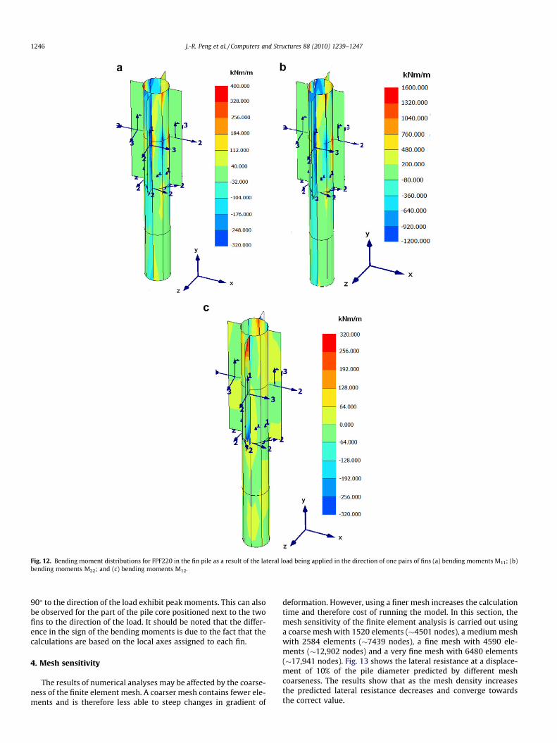
Fig. 12. Bending moment distributions for FPF220 in the fin pile as a result of the lateral load being applied in the direction of one pairs of fins (a) bending moments M11; (b)bending moments M22; and (c) bending moments M12.

1246 J.-R. Peng et al. / Computers and Structures 88 (2010) 1239–1247

90� to the direction of the load exhibit peak moments. This can alsobe observed for the part of the pile core positioned next to the twofins to the direction of the load. It should be noted that the differ-ence in the sign of the bending moments is due to the fact that thecalculations are based on the local axes assigned to each fin.

4. Mesh sensitivity

The results of numerical analyses may be affected by the coarse-ness of the finite element mesh. A coarser mesh contains fewer ele-ments and is therefore less able to steep changes in gradient of

deformation. However, using a finer mesh increases the calculationtime and therefore cost of running the model. In this section, themesh sensitivity of the finite element analysis is carried out usinga coarse mesh with 1520 elements (�4501 nodes), a medium meshwith 2584 elements (�7439 nodes), a fine mesh with 4590 ele-ments (�12,902 nodes) and a very fine mesh with 6480 elements(�17,941 nodes). Fig. 13 shows the lateral resistance at a displace-ment of 10% of the pile diameter predicted by different meshcoarseness. The results show that as the mesh density increasesthe predicted lateral resistance decreases and converge towardsthe correct value.

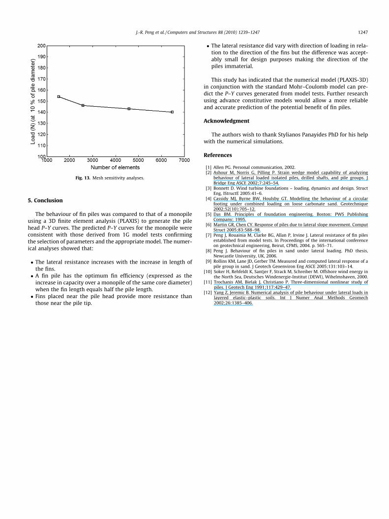
Fig. 13. Mesh sensitivity analyses.

J.-R. Peng et al. / Computers and Structures 88 (2010) 1239–1247 1247

5. Conclusion

The behaviour of fin piles was compared to that of a monopileusing a 3D finite element analysis (PLAXIS) to generate the pilehead P–Y curves. The predicted P–Y curves for the monopile wereconsistent with those derived from 1G model tests confirmingthe selection of parameters and the appropriate model. The numer-ical analyses showed that:

� The lateral resistance increases with the increase in length ofthe fins.� A fin pile has the optimum fin efficiency (expressed as the

increase in capacity over a monopile of the same core diameter)when the fin length equals half the pile length.� Fins placed near the pile head provide more resistance than

those near the pile tip.

� The lateral resistance did vary with direction of loading in rela-tion to the direction of the fins but the difference was accept-ably small for design purposes making the direction of thepiles immaterial.

This study has indicated that the numerical model (PLAXIS-3D)in conjunction with the standard Mohr–Coulomb model can pre-dict the P–Y curves generated from model tests. Further researchusing advance constitutive models would allow a more reliableand accurate prediction of the potential benefit of fin piles.

Acknowledgment

The authors wish to thank Stylianos Panayides PhD for his helpwith the numerical simulations.

References

[1] Allen PG. Personal communication, 2002.[2] Ashour M, Norris G, Pilling P. Strain wedge model capability of analyzing

behaviour of lateral loaded isolated piles, drilled shafts, and pile groups. JBridge Eng ASCE 2002;7:245–54.

[3] Bonnett D. Wind turbine foundations – loading, dynamics and design. StructEng, IStructE 2005:41–6.

[4] Cassidy MJ, Byrne BW, Houlsby GT. Modelling the behaviour of a circularfooting under combined loading on loose carbonate sand. Geotechnique2002;52(10):705–12.

[5] Das BM. Principles of foundation engineering. Boston: PWS PublishingCompany; 1995.

[6] Martin GR, Chen CY. Response of piles due to lateral slope movement. ComputStruct 2005;83:588–98.

[7] Peng J, Rouainia M, Clarke BG, Allan P, Irvine J. Lateral resistance of fin pilesestablished from model tests. In Proceedings of the international conferenceon geotechnical engineering, Beirut, CFMS, 2004. p. 565–71.

[8] Peng J. Behaviour of fin piles in sand under lateral loading. PhD thesis,Newcastle University, UK, 2006.

[9] Rollins KM, Lane JD, Gerber TM. Measured and computed lateral response of apile group in sand. J Geotech Geoenviron Eng ASCE 2005;131:103–14.

[10] Soker H, Rehfeldt K, Santjer F, Strack M, Schreiber M. Offshore wind energy inthe North Sea, Deutsches Windenergie-Institut (DEWI), Wihelmshaven, 2000.

[11] Trochanis AM, Bielak J, Christiano P. Three-dimensional nonlinear study ofpiles. J Geotech Eng 1991;117:429–47.

[12] Yang Z, Jeremic B. Numerical analysis of pile behaviour under lateral loads inlayered elastic–plastic soils. Int J Numer Anal Methods Geomech2002;26:1385–406.