BEHAVIOR OF PILES IN LATERALLY SPREADING GROUND DURING EARTHQUAKES - REPORT FOR PDS02

CENTER FOR GEOTECHNICAL MODELING REPORT NO. UCD/CGMDR-00/06

BEHAVIOR OF PILES IN LATERALLY SPREADING GROUND DURING EARTHQUAKES - REPORT FOR PDS02

BY P. SINGH R.W. BOULANGER B.L. KUTTER

Research supported by the California Department of Transportation under Contract Number 59A0162. The intention of this report is to make the data available to interested researchers. While great effort has been made to accurately report the results, the results herein are subject to revision. Please see the conditions and limitations within.

DEPARTMENT OF CIVIL & ENVIRONMENTAL ENGINEERING COLLEGE OF ENGINEERING UNIVERSITY OF CALIFORNIA AT DAVIS DECEMBER, 2000

i

BEHAVIOR OF PILES IN LATERALLY SPREADING GROUND DURING

EARTHQUAKES – CENTRIFUGE DATA REPORT FOR PDS02

P. Singh, R. W. Boulanger, and B. L. Kutter Center for Geotechnical Modeling Data Report UCD/CGMDR-00/06

Date: December, 2000 Date of testing: August, 2000 Project:

Behavior of Piles in Laterally Spreading Ground during Earthquakes

Contract number: 59A0162 Sponsor(s): Caltrans Previous reports in this test series:

UCD/CGM/DR-00/05

ACKNOWLEDGMENTS This model test was funded by Caltrans under the direction of Abbas Abghari. The contents of this report do not necessarily represent a policy of that agency nor endorsement by the state government. The authors would like to acknowledge the suggestions and assistance of Abbas Abghari, Hideo Nakajima, Dan Wilson, Chad Justice, Tom Coker, Tom Kohnke, and Tejasbaba. The model tests were performed using the large geotechnical centrifuge at UC Davis. Development of this centrifuge was supported primarily by the National Science Foundation, NASA and the University of California. Additional support was obtained from Tyndall Air Force Base, the Naval Civil Engineering Laboratory and Los Alamos National Laboratories. The large shaker was funded by the California Department of Transportation, the Obayashi Corporation, the National Science Foundation and the University of California. CONDITIONS AND LIMITATIONS Permission is granted for the use of these data for publications in the open literature, provided that the authors and sponsors are properly acknowledged. It is essential that the authors be consulted prior to publication to discuss errors or limitations in the data not known at the time of the release of this report. In particular, there may be later releases of this report. Questions about this report may be directed by email to [email protected].

TABLE OF CONTENTS

COVER PAGE ......................................................................................................................................................i

CONFIGURATION OF THE TEST ....................................................................................................................1

MODEL PREPARATION....................................................................................................................................2

SOIL PROPERTIES.............................................................................................................................................2

PILE PROPERTIES .............................................................................................................................................5

SCALE FACTORS...............................................................................................................................................5

ORGANIZATION OF PLOTS FROM DATA ACQUISITION SYSTEM..........................................................6

INSTRUMENTATION AND MEASUREMENTS .............................................................................................8

KNOWN LIMITATIONS OF RECORDED DATA AND MODEL..................................................................13

REFERENCES ..................................................................................................................................................14

APPENDIX A: DESCRIPTION OF CENTRIFUGE FACILITIES .................................................................A-1

1

CONFIGURATION OF THE TEST This is the second test in a series to study the behavior of pipe piles in laterally spreading ground during earthquakes. This test focuses on the interaction of a pile-group and soil during lateral spreading. A pile group, consisting of six piles of 0.69-m outer-diameter prototype steel pipe piles, was modeled using aluminum tubing of diameter 1.9 cm (0.75 in.) and aluminum pile cap. The soil profile was prepared with a 0.75 cm thick coarse sand layer, an 11-cm thick deposit of over-consolidated clay overlying a 11.5-cm thick loose sand (Dr= 28%) layer, overlying dense sand (Dr = 83%). All of the layers were built to a slope of 3o. A �river� channel was cut through the surface deposit across the short dimension (east-west direction) of the model container at the north end of the container. The riverbank was built at a slope of 25o. Model container FSB2 was used. The model layout is shown in Figure 1. A total of three shaking events were applied to the model at a centrifugal acceleration of 36.2 g. The shaking was applied transverse to the river channel in the north-south direction. Two of the three shaking events consisted of scaled versions of the ground motion recorded at 80 m depth at Port Island in the 1995 Great Hanshin Awaji Earthquake. The shaking events in this test were numbered as PDS02_01 through PDS02_03. The sequence of motions is tabulated in Table 1. Centrifuge: 9 m radius centrifuge at UC Davis Model Container: Flexible Shear Beam 2 (FSB2) Centrifugal Acceleration: 36.2 g Pore Fluid: Water Table 1:Ground Motion Sequence

Event ID Name of Motion Peak Base Acc.

Model (g)

Time Date Input Motion

File

Amp. Factor

D to A Freq. (Hz)

Spin up --- 13:25 8/03/00 --- --- --- PDS02_01 Step Wave 1.7 16:45 8/03/00 Step 2.0 4000 Spin down --- 16:55 8/03/00 --- --- ---

Spin up --- 18:38 8/03/00 --- --- --- PDS02_02 Small Kobe 14 21:54 8/03/00 Kobe0807 2.2 2000 PDS02_03 Large Kobe 60 22:33 8/03/00 Kobe0807 7.0 2000 Spin down --- 00:30 8/04/00 --- --- ---

2

MODEL PREPARATION The dense and loose sand layers were placed by dry pluviation. A barrel pluviator was used to achieve 28% relative density in the loose sand layer. Slurry consisting of reconstituted bay mud was prepared with a mixer, placed on the loose sand surface, and a consolidation press was used to consolidate the clay layer. A vacuum pressure of 10 kPa was applied at the bottom of the container to remove any water that may have entered the sand layer due to consolidation of the clay. The clay layer was placed and consolidated in two lifts under a vertical stress of 100 kPa. After consolidation, the river channel was carved into the required slope with the help of a thin metal wire. The model was then flooded with CO2 gas and placed under a vacuum of 25 in. Hg in order to remove the air in the sand. Water was dripped slowly in to the evacuated model until the water level reached the desired height, which required approximately 13 hours. A 0.75 cm thick layer of Monterey sand was spread on top of clay to protect it from drying. A sheet-aluminum rectangle with dimensions 25.5 X 15.5 X 6 cm, was pressed into the clay, and the clay inside of the rectangle was excavated. Piles were driven using a drop hammer. Each pile was driven in 5 cm at a time, and the pile cap was progressively slid down over the piles as they were driven. A plumb line and spirit level were used to ensure that piles were driven in vertically. The bucket was tilted at an angle of 0.75o to ensure that the piles were close to vertical during the shakes. The bucket was at an angle of 1.2o from the horizontal while spinning. The pile cap was lowered into the excavation, such that it was horizontal and its top was flush with the clay surface on the southern side. Plaster was placed in between the pile cap and sheet-aluminum rectangle. Thus the effective dimensions of the pile cap were 25.5 X 15.5 X 6 cm. SOIL PROPERTIES Some of the soil properties of the sand and clay are summarized in Table 2. The range in relative density is based on the variability in repeated maximum and minimum density measurements according to ASTM D4253-83 and D4254-83. A Dr of 28% for the loose sand and 83% for the dense sand is obtained using data by Woodward-Clyde (1997), which were the standards used in this test, and a Dr of 26% for loose sand and 70% for dense sand is obtained using data by Earth Technology Corporation (Arulmoli et at. 1991).

3

Table 2: Some properties of the soils Parameter

Dense Sand

Layer Loose Sand

Layer Clay layer

Soil type Nevada sand Nevada sand Bay Mud Specific gravity1 2.644 2.644 2.65 Mean grain size, D50 (mm) 0.17 0.17 - Coefficient of uniformity, CU 1.64 1.64 - Maximum dry unit weight, γmax (kN/m3) 16.79-17.33 16.79-17.33 - Minimum dry unit weight, γmin (kN/m3) 13.87-14.0 13.87-14.0 - Relative density (%) 70-83 26-28 - Saturated unit weight (kN/m3) 20.0 19.1 15.5 Permeability2 (cm/sec) 3.2 x 10-3 - - PL - - 35-40 LL - - 88-93 Pre-consolidation pressure (kPa) - - 100 Water content (after consolidation) (%) - - 62.9-63.7 Undrained shear strength, cu (after consolidation) (kPa)

- - 15-18

Shear wave velocities were measured in flight at 38.1 g using horizontal shear wave hammers consisting of a ball bearing inside an evacuated metal tube. The ball bearing moves from one side of the tube to the other when the vacuum pressure on one side of the tube is changed, which generates a vertically propagating shear wave. Measured velocities are presented in Table 3. Shear wave velocities in the intervals A7 � A8 and A8 � A9 could not be determined because instrument A8 moved east from its location. Table 3: Shear Wave Velocities

Accelerometer Interval

Depth Interval

(cm)

Vertical Distance Between

Accelerometers (cm)

Soil Type Average Shear Wave

Velocity (m/s)

A5 - A6 58.4 - 34.4 24 Dense Sand 240 A6 - A7 34.4 - 28.4 6.0 Dense Sand 241 A7 - A9 28.4 - 19.1 9.3 Loose Sand 134

The p-wave velocities were measured at 1-g prior t spin-up to determine the degree of saturation of the model. The average p-wave velocity in the model was measured to be 800 m/s. The p-wave velocity is expected to increase during spin-up due to the increase in solubility of air into water at increased pressure. A pocket torvane was used to measure the shear strength of clay. Shear strengths, measured after consolidation of the first layer of clay, varied from 15 kPa on south side of the slope, to 18 kPa on north side. The shear strength obtained after the second lift was 18 kPa. Shear 1 Cruz (1995) and Chen (1995) 2 Chen (1995)

4

strengths of 17.2 � 20 kPa were obtained in 4 tests after the end of centrifuge testing. These results are summarized in Table 4. Water content results for clay are summarized in Table 5. Table 4(a): Vane-shear tests after consolidation 1. Shear strengths after consolidation of first lift

x (cm) y (cm) Cu (kPa) 40 20 18

82.5 20 18 120 20 15

2. Shear strengths after consolidation of second lift x (cm) y (cm) Cu (kPa)

40 20 18 82.5 20 18 120 20 18

Table 4(b): Vane-shear tests after the shaking events

Location x (cm) y (cm) Depth (cm)

Cu (kPa)

115 23 03 18 115 23 1.5 20 115 23 3.1 17.2 115 23 7.0 20

Notes: Vane shear tests were performed between 2 to 2.5 hours after start of spin down. Depth is measured from top of the clay surface. X and Y coordinates are measured from the top north-west corner of the container to approximately the center of the vane-shear test pits. Table 5: Water content of clay

Time Water Content (%)

After consolidation: first lift 63.7 After consolidation: second lift 62.9

After the shaking events 69.2 After the shaking events 70.3

T-bar (bar penetrometer) tests were also performed on clay after the spinning down. A T-bar of diameter 9 mm and length 31 mm was used for the tests. The results are presented in Table 6. These results are based on a bar factor value of 10.5, as recommended by Randolph and Houlsby (1984). Details of the bar penetrometer testing are presented in Stewart and Randolph (1991).

5

Table 6: Shear strength of clay after spinning down, using the T-bar device Shear strength (kPa)

Site 1 Site 2 Depth (cm) (x, y) cm = (110, 40) (x, y) cm = (145, 60)

0.64 7.9 10.7 1.27 8.2 10.7 1.91 8.9 11.1 2.54 9.0 11.3 3.18 9.5 10.4 3.81 10.7 9.8 4.45 11.0 10.1 5.08 13.7 10.4 5.72 14.7 11.0 6.35 14.7 11.3 6.99 14.7 11.3 7.62 14.3 10.5 8.25 13.4 10.7 8.89 12.8 11.0 9.53 13.1 11.6

10.16 13.7 12.1 Notes: Depth is measured from the top of clay surface. PILE PROPERTIES A pile-group of six piles, each of outer diameter 1.91 cm and wall thickness 0.09 cm, made of aluminum 6061-T6, was tested in PDS02. The piles have Young�s Modulus, E = 68.9 Gpa, and yield strength, σyield of 216 Mpa. Three of these piles were made by modifying the piles used for PDS01. All piles except the pile on the south-west corner of the group were 41 cm long below the pile-cap. The pile on the south-west corner extended 43 cm below the pile cap in order to accommodate a strain gauge. Strain gages were affixed to three piles to measure the bending moments (Figures 2 to 4). The other three piles were equipped with strain gages to measure the axial and shear strains (Figures 5). The pile cap for pile group was made of Aluminum, and was of the dimensions 24 X 14 X 6 cm. (Figure 6). The piles were covered by shrink-wrap to prevent gauges from getting wet. Pile tips were made of plastic and the tip angle was 60o. SCALE FACTORS All data presented in this report is in prototype scale, unless otherwise explicitly stated. Table 7 lists factors that were used to convert the data to prototype scale. Table 7: Scale factors used to convert the model data to prototype units

Quantity Prototype Dimension / Model Dimension Time (dynamic) 36.2/1

Displacement, Length 36.2/1 Acceleration, Gravity 1/36.2

Pressure, Stress 1/1 Permeability *

*The permeability of the prototype soil would be 36.2 times greater than that indicated in Table 2.

6

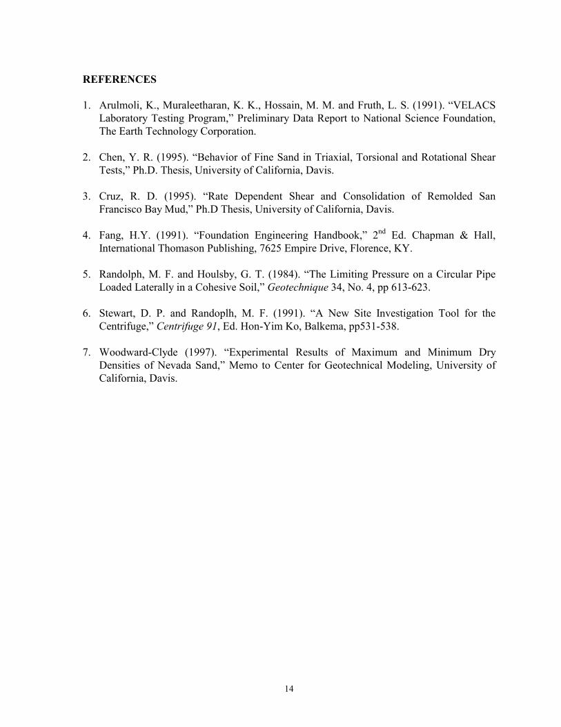
ORGANIZATION OF PLOTS FROM DATA ACQUISITION SYSTEM The data for the shaking events (refer to Table 1 for event names) is reproduced on 18 pages of time histories as described in Table 8. The first set of plots is for the Step wave. Note that some of the instruments do not record a strong enough response, to the Step wave, to be seen above the instrument noise level. Data from PDS02_02 was recorded for a period of 9 seconds at three different sampling frequencies. Data was collected at 2000 Hz for 1 second, 200 Hz for next 2 seconds, and at 20 Hz for the remaining 6 seconds. However, only the first second of data has been plotted since the shaking takes place during this time. The lowermost plot on each page is the base acceleration for that shaking event. Note that the scale for the base acceleration is the same as all of the accelerometers, but that the scale for the base acceleration is not correct when plotted with all other non-acceleration data. The �units-per-tick� definition doesn�t apply to the base acceleration record when plotted with non-acceleration data, and the base acceleration is included simply as a time reference. Table 8: Organization of data

Instrument Number Description Page

P1, P3, P4 Vertical pore-pressure array: north of pile-group 1 P5 � P10 Vertical pore-pressure array: south of pile-group 2

P11 � P14 Pore pressures in loose sand, around the pile-group 3 A1 � A4 Vertical array of horizontal accelerations: north of pile-group 4

A5 � A10 Vertical array of horizontal accelerations: south of pile-group 5 A11, A15, A16, A17 Accelerations in loose sand, east and west shakers, and on ring 2 of the

model container 6

A12 � A14 Vertical array of vertical accelerations 7 NWM2 � NWM6 Moments in north-west pile 8

NWM7 � NWM11 Moments in north-west pile 8a NEA1, NES2, NES3,

NEA4 Axial and shear loads in north-east pile 9

CWA1, CWS2, CWS3, CWA4

Axial and shear loads in central-west pile 10

CEM2 � CEM5 Moments in central-east pile 11 SWM2 � SWM7 Moments in south-west pile 12

SWM8 � SWM12 Moments in south-west pile 12a SEA1, SES2, SES3,

SEA4 Axial and shear loads in south-east pile 13

L1, L2, L13, L14 Displacements of ring 2 and 3 of container, horizontal displacement of pile group

14

L3 � L5, L8, L9 Horizontal displacement of clay 15 L6, L7, L10 � L12 Vertical displacement of clay and pile cap 16 Notation: A � Accelerometer P � Pore water pressure transducer L � Displacement Transducer NWM, CEM, SWM � Moment gauge (full) bridge on north-west, central-east or south-west pile NEA, CWA, SEA � Axial gauge (full) bridge on north-east, central-west or south-east pile NES, CWS, SES � Shear gauge (full) bridge on north-west, central-east or south-west pile

7

Data of PDS02_03 was lost as the online computer froze before the data could be written to a file. However, the readings before and after the shake were recorded, and are presented in Table 9. Table 9. Instrument readings before and after PDS02_03

Instrument Before PDS02_03 After PDS02_03 Difference Units NWM2 -1517.19 -1786.59 -269.40 kN-m NWM3 -1000.65 -1204.58 -203.93 kN-m NWM4 -8.82 -168.69 -159.86 kN-m NWM5 -0.75 -82.51 -81.76 kN-m NWM6 1.37 31.26 29.88 kN-m NWM7 -7.90 83.04 90.94 kN-m NWM8 -5.84 160.91 166.75 kN-m NWM9 -8.01 190.40 198.41 kN-m

NWM10 7.80 188.97 181.17 kN-m NWM11 8.48 135.47 126.99 kN-m CEM2 4.64 -141.43 -146.06 kN-m CEM3 4.30 -154.18 -158.48 kN-m CEM4 7.10 -21.16 -28.26 kN-m CEM5 -5.35 29.12 34.47 kN-m SWM2 2.53 -168.56 -171.09 kN-m SWM3 4.01 -180.41 -184.41 kN-m SWM4 -2.36 -201.23 -198.87 kN-m SWM5 6.19 -184.41 -190.60 kN-m SWM6 -4.36 -146.96 -142.59 kN-m SWM7 -1.31 -61.93 -60.62 kN-m SWM8 1.86 11.07 9.21 kN-m SWM9 -0.08 60.10 60.18 kN-m

SWM10 6.08 196.24 190.16 kN-m SWM11 -7.88 171.24 179.13 kN-m SWM12 0.57 27.45 26.87 kN-m NEA1 5.43 -159.60 -165.02 kN NES2 0.75 139.76 139.02 kN NES3 -0.44 49.81 50.25 kN NEA4 6.12 90.10 83.98 kN CWS2 1.65 24.59 22.94 kN CWS3 -0.31 34.70 35.00 kN CWA4 -0.95 211.72 212.67 kN SEA1 -2.69 259.06 261.75 kN SES2 -5.01 -21.00 -15.99 kN SES3 -2.43 33.25 35.68 kN SEA4 -6.56 12.91 19.47 kN

L1 -0.54 9.43 9.97 mm L2 -2.08 -2.17 -0.09 mm L3 0.12 -952.54 -952.67 mm L4 -0.90 -1.21 -0.31 mm L5 0.94 -461.31 -462.25 mm L6 0.47 642.82 642.34 mm L7 -0.40 -646.09 -645.69 mm L8 0.38 559.88 559.50 mm L9 0.33 843.33 843.00 mm

L10 0.16 580.86 580.70 mm L11 -0.47 -55.33 -54.85 mm L12 0.29 89.97 89.68 mm L13 1.66 515.87 514.21 mm L14 -0.66 535.47 536.13 mm

Note: The readings after PDS02_03 were recorded approximately an hour after the shaking.

8

INSTRUMENTATION AND MEASUREMENTS The centrifuge facilities and instrumentation system are briefly described in Appendix A. Instrumentation and facilities used in this test but not described in Appendix A are described below. All of the accelerometers were placed pointing south. Accelerometers were oriented such that a positive acceleration is towards the north end of the container. Linear potentiometers and LVDTs were placed as shown in Figure 1. For linear potentiometers, a negative displacement refers to a retraction of the shaft of the instrument into the housing, and a positive displacement refers to an extension of the shaft out of the housing. LVDTs follow an opposite sign convention. In the model, L13 and L14 are LVDTs and L1 through L12 are linear potentiometers. Table 10 shows the position of the piles with reference to the top-north-west corner of the model. The initial locations of the instruments with their sensitivity, channel numbers and channel gains are given in Table 11. The coordinates for the instrument locations, listed in Table 11(a) are referenced from the top-north-west corner of the model container. Locations of strain gauges on any pile are referenced from the bottom tip of the respective pile. The instrument locations of the model are shown in Figure 1. Piles with strain gauges are shown in Figures 2 to 5. Table 10: Location of pile tips with respect to the origin (top-north-west corner of container)

Pile X (cm) Y (cm) Z (cm) NE 58 35.4 55.4 NW 58 43.4 55.4 CE 66 35.4 55.4 CW 66 43.4 55.4 SE 74 35.4 55.4 SW 74 43.4 57.4

Notes: Location of strain gauges on the piles is measured with bottom tip of the piles as reference.

9

Table 11(a): Instrumentation Details - pore pressure transducers, accelerometers, displacement transducers * Instrument locations are measured from top-North-West corner of the container

Instrument Location*

Instr. Instr. Instr. x y z Instr. Sensitivity Bucket DT Calib. Factor Calib. Factor

Name Type No. (cm) (cm) (cm) Range & Units Gain Gain w/o DT Gain Prototype

P1 PWP 10041 30 39.4 58.4 100 psi 8110 kPa/V 100 2 81.10 kPa/V 81.10 kPa/V

P2 PWP 7368 31 39 36.3 50 psi 3976 kPa/V 100 2 39.76 kPa/V 39.76 kPa/V

P3 PWP 1330 26.9 37.2 25.23 50 psi 3758 kPa/V 100 2 37.58 kPa/V 37.58 kPa/V



P6 PWP 7370 114.2 39 34.6 50 psi 3900 kPa/V 100 2 39.00 kPa/V 39.00 kPa/V




P10 PWP 10034 90 27 12 100 psi 8224 kPa/V 100 2 82.24 kPa/V 82.24 kPa/V





L1 Displ 202 Ring 2, south end 2" 5.04 mm/V 1 2 5.04 mm/V 182.34 mm/V

L2 Displ 212 Ring 3, south end 2" 5.11 mm/V 1 2 5.11 mm/V 184.84 mm/V

L3 Displ 207 Horizontal, south-east of pile-gr. 2" 5.07 mm/V 1 2 5.07 mm/V 183.53 mm/V

L4 Displ 209 Horizontal, south of pile-gr. 2" 5.06 mm/V 1 2 5.06 mm/V 183.03 mm/V

L5 Displ 211 Horizontal, south-west of pile-gr. 2" 5.08 mm/V 1 2 5.08 mm/V 183.79 mm/V

L6 Displ 214 Vertical, south-east of pile-gr. 2" 5.06 mm/V 1 2 5.06 mm/V 183.24 mm/V

L7 Displ 201 Vertical, south-west of pile-gr. 2" 5.06 mm/V 1 2 5.06 mm/V 183.03 mm/V

L8 Displ 419741 Horizontal, north-east of pile-gr. 2" 5.75 mm/V 1 2 5.75 mm/V 208.15 mm/V

L9 Displ 419740 Horizontal, north-west of pile-gr. 2" 5.92 mm/V 1 2 5.92 mm/V 214.27 mm/V

L10 Displ 401 Vertical, north-east of pile-gr. 4" 10 mm/V 1 2 10.04 mm/V 363.30 mm/V

L11 Displ 102 Vertical, on south end of pile cap 1" 2.52 mm/V 1 2 2.52 mm/V 91.22 mm/V

L12 Displ 101 Vertical, on north end of pile cap 1" 2.54 mm/V 1 2 2.54 mm/V 91.95 mm/V

L13 Displ 419167 Horizontal, on NW pile 2" 6.09 mm/V 1 2 6.09 mm/V 220.57 mm/V

L14 Displ 469051 Horizontal, on NE pile 2" 6.16 mm/V 1 2 6.16 mm/V 222.92 mm/V

A1 Acc 21043 40 39.4 58.4 100g 19.1 g/V 1 2 19.08 g/V 0.53 g/V

A2 Acc 21055 40.4 36.5 33.88 100g 19.5 g/V 1 2 19.49 g/V 0.54 g/V

A3 Acc 21323 41.4 37.3 24.75 100g 21.3 g/V 1 2 21.28 g/V 0.59 g/V

A4 Acc 5599 40 37.6 14 100g 19.1 g/V 1 2 19.05 g/V 0.53 g/V

A5 Acc 21044 100 38.6 58.4 100g 18.6 g/V 1 2 18.62 g/V 0.51 g/V

A6 Acc 21056 101.3 38.1 34.46 100g 18.2 g/V 1 2 18.25 g/V 0.50 g/V

A7 Acc 21063 102.6 42.8 28.46 100g 19.8 g/V 1 2 19.76 g/V 0.55 g/V

A8 Acc 21319 -- -- -- 100g 19.2 g/V 1 2 19.16 g/V 0.53 g/V

A9 Acc 21051 100.3 40.5 19.09 100g 19.2 g/V 1 2 19.19 g/V 0.53 g/V

A10 Acc 21061 100 39.6 11 100g 20.2 g/V 1 2 20.20 g/V 0.56 g/V

A11 Acc 21071 61.4 59.1 22.81 100g 18.8 g/V 1 2 18.83 g/V 0.52 g/V

A12 Acc 21046 130 39 43.99 100g 18.7 g/V 1 2 18.73 g/V 0.52 g/V

A13 Acc 21065 130.4 39.5 34.53 100g 18.2 g/V 1 2 18.18 g/V 0.50 g/V

A14 Acc 21322 134.8 38 20.85 100g 20 g/V 1 2 19.96 g/V 0.55 g/V

A15 Acc 3202 North-East, Shaker Table 50g 9.71 g/V 1 2 9.71 g/V 0.27 g/V

A16 Acc 3948 North-West, Shaker Table 50g 9.45 g/V 1 2 9.45 g/V 0.26 g/V

A17 Acc 5276 Container, Ring -2 50g 9.56 g/V 1 2 9.56 g/V 0.26 g/V

10

Table 11(b): Instrumentation Details - Strain Gauges * Locations of strain gauges are measured upwards from bottom of the pile those are installed on.

Location* Instr. Instr. z Sensitivity Bucket DT Calib. Factor Calib. Factor Name Type (cm) & Units Gain Gain w/o DT Gain Prototype

NWM1 Moment 39.7 0.000057 V/lb-in 100 2 0.02 kN-m/V 940.6 kN-m/V NWM2 Moment 36.4 0.000057 V/lb-in 100 2 0.02 kN-m/V 940.6 kN-m/V NWM3 Moment 33.1 0.000057 V/lb-in 100 2 0.02 kN-m/V 940.6 kN-m/V NWM4 Moment 29.7 0.000057 V/lb-in 100 2 0.02 kN-m/V 940.6 kN-m/V NWM5 Moment 25.6 0.000057 V/lb-in 100 2 0.02 kN-m/V 940.6 kN-m/V NWM6 Moment 21.5 0.000057 V/lb-in 100 2 0.02 kN-m/V 940.6 kN-m/V NWM7 Moment 17.2 0.000057 V/lb-in 100 2 0.02 kN-m/V 940.6 kN-m/V NWM8 Moment 14.7 0.000057 V/lb-in 100 2 0.02 kN-m/V 940.6 kN-m/V NWM9 Moment 12.2 0.000057 V/lb-in 100 2 0.02 kN-m/V 940.6 kN-m/V

NWM10 Moment 9.7 0.000057 V/lb-in 100 2 0.02 kN-m/V 940.6 kN-m/V NWM11 Moment 6 0.000057 V/lb-in 100 2 0.02 kN-m/V 940.6 kN-m/V SWM1 Moment 41.5 0.000057 V/lb-in 100 2 0.02 kN-m/V 940.6 kN-m/V SWM2 Moment 39 0.000057 V/lb-in 100 2 0.02 kN-m/V 940.6 kN-m/V SWM3 Moment 36.5 0.000057 V/lb-in 100 2 0.02 kN-m/V 940.6 kN-m/V SWM4 Moment 34 0.000057 V/lb-in 100 2 0.02 kN-m/V 940.6 kN-m/V SWM5 Moment 29.9 0.000057 V/lb-in 100 2 0.02 kN-m/V 940.6 kN-m/V SWM6 Moment 25.8 0.000057 V/lb-in 100 2 0.02 kN-m/V 940.6 kN-m/V SWM7 Moment 21.5 0.000057 V/lb-in 100 2 0.02 kN-m/V 940.6 kN-m/V SWM8 Moment 19 0.000057 V/lb-in 100 2 0.02 kN-m/V 940.6 kN-m/V SWM9 Moment 16.5 0.000057 V/lb-in 100 2 0.02 kN-m/V 940.6 kN-m/V

SWM10 Moment 14 0.000057 V/lb-in 100 2 0.02 kN-m/V 940.6 kN-m/V SWM11 Moment 10.3 0.000057 V/lb-in 100 2 0.02 kN-m/V 940.6 kN-m/V SWM12 Moment 4 0.000057 V/lb-in 100 2 0.02 kN-m/V 940.6 kN-m/V CEM1 Moment 39.5 0.000057 V/lb-in 100 2 0.02 kN-m/V 940.6 kN-m/V CEM2 Moment 34.5 0.000057 V/lb-in 100 2 0.02 kN-m/V 940.6 kN-m/V CEM3 Moment 25.4 0.000057 V/lb-in 100 2 0.02 kN-m/V 940.6 kN-m/V CEM4 Moment 17 0.000057 V/lb-in 100 2 0.02 kN-m/V 940.6 kN-m/V CEM5 Moment 12 0.000057 V/lb-in 100 2 0.02 kN-m/V 940.6 kN-m/V NEA1 Axial 40 0.000010 V/lb 500 2 0.91 kN/V 1190.0 kN/V NES2 Shear 39 0.000034 V/lb 500 2 0.26 kN/V 343.0 kN/V NES3 Shear 24 0.000034 V/lb 500 2 0.26 kN/V 343.0 kN/V NEA4 Axial 23 0.000010 V/lb 500 2 0.91 kN/V 1190.0 kN/V CWA1 Axial 40 0.000010 V/lb 500 2 0.91 kN/V 1190.0 kN/V CWS2 Shear 39 0.000034 V/lb 500 2 0.26 kN/V 343.0 kN/V CWS3 Shear 24 0.000034 V/lb 500 2 0.26 kN/V 343.0 kN/V CWA4 Axial 23 0.000010 V/lb 500 2 0.91 kN/V 1190.0 kN/V SEA1 Axial 40 0.000010 V/lb 500 2 0.91 kN/V 1190.0 kN/V SES2 Shear 39 0.000034 V/lb 500 2 0.26 kN/V 343.0 kN/V SES3 Shear 24 0.000034 V/lb 500 2 0.26 kN/V 343.0 kN/V SEA4 Axial 23 0.000010 V/lb 500 2 0.91 kN/V 1190.0 kN/V

11

The electronic data for this test are contained in two ASCI files: pds02_01.prn Step wave pds02_02.prn Small Kobe For these files, the columns and corresponding instruments are summarized in Table 12. Due to malfunctioning of certain accelerometers or the channels these were plugged into, the channel list was changed after the Step wave. Table 12: Channel list for the events PDS02_01 and PDS02_02.

Column No. Step Wave (PDS02_01) Small Kobe (PDS02_02) 0 Time Time 1 P14 P14 2 NWM2 NWM2 3 NWM3 NWM3 4 NWM4 NWM4 5 NWM5 NWM5 6 NWM6 NWM6 7 NWM7 NWM7 8 NWM8 NWM8 9 NWM9 NWM9

10 NWM10 NWM10 11 NWM11 NWM11 12 SEA1 SEA1 13 SES2 SES2 14 SES3 SES3 15 SEA4 SEA4 16 NEA1 NEA1 17 NES2 NES2 18 NES3 NES3 19 NEA4 NEA4 20 P8 P8 21 CWS2 CWS2 22 CWS3 CWS3 23 CWA4 CWA4 24 SWM5 SWM5 25 SWM6 SWM6 26 SWM7 SWM7 27 SWM8 SWM8 28 SWM9 SWM9 29 SWM10 SWM10 30 SWM11 SWM11 31 SWM12 SWM12 32 L1 L1 33 L2 L2 34 L3 L3 35 L4 L4 36 L5 L5 37 L6 L6 38 L7 L7 39 L8 L8

12

40 L9 L9 41 L10 L10 42 L11 L11 43 L12 L12 44 L13 L13 45 L14 L14 46 P9 P9 47 P10 P10 48 P13 P13 49 SWM2 SWM2 50 SWM3 SWM3 51 SWM4 SWM4 52 P12 P12 53 CEM2 CEM2 54 CEM3 CEM3 55 CEM4 CEM4 56 CEM5 CEM5 57 P1 P1 58 P11 P11 59 P3 P3 60 P4 P4 61 P5 P5 62 P6 P6 63 P7 P7 64 A1 A1 65 A2 A2 66 A3 A3 67 A4 A4 68 A5 A5 69 A6 A6 70 A7 A7 71 A8 A8 72 A9 A9 73 A10 A10 74 A11 A15 75 A12 A16 76 A13 A17 77 A14 A14 78 A15 A11 79 A16 A12 80 A17 A13

Vertical black sand columns were put in sand to observe the deformation pattern. Noodles were used to observe the relative movement between clay and sand, and to observe if any strain was generated within the clay layer. A horizontal strip of black sand was put in loose sand to observe the effect of the pile group on the loose sand. Flexible chains were used to measure displacement and deformation pattern at the top of the clay. Figures 7 to 9 show these markers before and after the test.

13

KNOWN LIMITATIONS OF RECORDED DATA AND MODEL The shaker did not send a signal back to the onboard computer after the big Kobe shake. The onboard computer froze, and was shut down. The data for PDS02_03 was not saved to a file, and was lost. Only the final offsets of the instruments after an hour of the shake could be recorded, when the onboard computer was re-booted. The second big Kobe shake, PDS02_04, was planned but could not take place since the shaker was not responding. The shear strength of clay recorded after the centrifuge test may not be indicative of the clay strength after shaking since the vane-shear and T-bar tests were performed approximately 2 hours after spinning down. All acceleration time histories in the electronic data files are raw recordings. Proper filtering and signal processing is required to obtain velocities, transient displacements, and other features of the dynamic response. Some instruments show a change in the steady voltage signal when the sampling frequency is changed (i.e. after shaking, as described previously). These �steps� in the data should be ignored. The vacuum chamber used during consolidation in the mechanical press was found to be empty of water. Around 19 gallons of water, which came out of the clay during consolidation, was retained in the sand, whereas it should have been drawn into the vacuum chamber. This could have obstructed uniform saturation of the sand. Instruments NWM1, CWA1, CEM1, and SWM1 were found to have big offsets when plugged into in the amplifier channels. This could be due to the loads generated by tightening the pile cap. It may be noted that these gauges were placed only 1 cm below the cap, and it was difficult to place the cap exactly since it was sitting in the excavation in clay. These four instruments were not plugged in during the test. Instruments A14, A15, A16 and A17 gave erroneous data after the Step wave. These instruments were thus replaced and the new instruments were also plugged into different amplifier channels. The channel gain list was subsequently changed. Location of A8 could not be determined since the instrument moved after the measurements were made, and the location was not re-measured. L10, the vertical linear pot on clay, did not work properly during PDS02_02. Instrument L2 did not show any recorded motion during PDS02_02, and was probably dead.

14

REFERENCES 1. Arulmoli, K., Muraleetharan, K. K., Hossain, M. M. and Fruth, L. S. (1991). �VELACS

Laboratory Testing Program,� Preliminary Data Report to National Science Foundation, The Earth Technology Corporation.

2. Chen, Y. R. (1995). �Behavior of Fine Sand in Triaxial, Torsional and Rotational Shear

Tests,� Ph.D. Thesis, University of California, Davis. 3. Cruz, R. D. (1995). �Rate Dependent Shear and Consolidation of Remolded San

Francisco Bay Mud,� Ph.D Thesis, University of California, Davis. 4. Fang, H.Y. (1991). �Foundation Engineering Handbook,� 2nd Ed. Chapman & Hall,

International Thomason Publishing, 7625 Empire Drive, Florence, KY. 5. Randolph, M. F. and Houlsby, G. T. (1984). �The Limiting Pressure on a Circular Pipe

Loaded Laterally in a Cohesive Soil,� Geotechnique 34, No. 4, pp 613-623. 6. Stewart, D. P. and Randoplh, M. F. (1991). �A New Site Investigation Tool for the

Centrifuge,� Centrifuge 91, Ed. Hon-Yim Ko, Balkema, pp531-538. 7. Woodward-Clyde (1997). �Experimental Results of Maximum and Minimum Dry

Densities of Nevada Sand,� Memo to Center for Geotechnical Modeling, University of California, Davis.

1.2° North South

165

A17

L 3-5L 13,14

A11 A14

A13

A12

78.7

A5

A6

A7

A10

A1

A2

A3A8A9

A11

A 5-10A 1-4 A12, 13, 14

A4 P10

P3

P2

P12P4 P11

P13P14

P9P8

P7

P6

P5P1

P11

P14 P 5-9

P 1-4

P12

P13, 10

L12

L11

L9

L13

L14

L10

L8

L5

L7

L4

L6

L3

L 1,2

DenseSand

LooseSand

ClayL 8,9

L2

L1

All dimensions in cm

Figure 1: PDS02 Layout

L 6,7L11L12

24

Monterey Sand


Figure 2: North-West pile

4.1

3.7

4.3

2.5

2.5

4.1

2.5

6

Pile cap

Outer Diameter 1.91 cmWall thickness 0.09 cm

3.3

3.3

3.4

Figure 3: Central-East pile

9.1

8.4

12

5


Pile cap

5

41

56


Figure 4: South-west pile


Pile cap

4.1

4


3.7

6.3

2.5

4.3

2.5

2.5

2.5

2.5

4.1

2.5

Shear gauge

Axial gauge

Shear gauge

Axial gauge

24

41 40

Figure 5: Axial and Shear Gauges on North-East, Central-West, and South-East piles

Outer diameter 1.91 cmWall thickness 0.09 cm

Pile cap

63


1

1

15

4

12

20

2.1

5.9

10.1

13.9

18.1

21.924 25

.7

6

3

1

1411

3

Figure 6: Pile cap

Aluminum sheet

South

Origin

North

Figure 7: Cross-section west of pile group (approximately at y = 20 cm) showing movement of noodles in clay and loose sand

Position of noodles before the test

Position of noodles after the test

xx/20

Scale: 0 to x: 25 cm (model scale)

South

Origin

North

Figure 8: Cross-section at center (approximately at y = 39 cm) showing clay and loose sand deformation pattern

Position of black sand columns after the test

Position of noodles before the test

Position of black sand columns before the test

Position of noodles after the test

x/2 xScale: 0 to x: 25 cm

0

Figure 9: Deformation pattern in clay using chain markers, and in loose sand using black sand strip

Chains in Clay, Before Test

Chains in Clay, After Test

Black Sand Strip in Sand, Before Test

Black Sand Strip in Sand, After Test

Scale: 0 to x: 25 cm (model scale)

0 x/2 x

DATA PLOTS:

PDS02

each_tick 0.45= inst_from_top "P4" "P3" "P1" "AB"( )=units

0 5 10 15 20 25 30 35Time (sec)

Lege

nd a

nd sc

ale

abov

epk_to_pk 2.22 2.11 3.37 1.22( )=

file "PDS02_01.prn"= page "1"=

each_tick 0.79= inst_from_top "P10" "P9" "P8" "P7" "P6" "P5" "AB"( )=units

0 5 10 15 20 25 30 35Time (sec)

Lege

nd a

nd sc

ale

abov

epk_to_pk 3.01 2.07 1.36 2.22 2.09 3.72 1.22( )=


each_tick 0.47= inst_from_top "P14" "P13" "P12" "P11" "AB"( )=units

0 5 10 15 20 25 30 35Time (sec)

Lege

nd a

nd sc

ale

abov

epk_to_pk 3.25 1.73 1.52 1.57 1.22( )=


each_tick 0.18= inst_from_top "A4" "A3" "A2" "A1" "AB"( )=units

0 5 10 15 20 25 30 35Time (sec)

Lege

nd a

nd sc

ale

abov

epk_to_pk 0.97 0.77 0.57 0.45 0.87( )=


each_tick 0.27= inst_from_top "A10" "A9" "A8" "A7" "A6" "A5" "AB"( )=units

0 5 10 15 20 25 30 35Time (sec)

Lege

nd a

nd sc

ale

abov

epk_to_pk 1.43 0.79 0.75 0.57 0.50 0.40 0.87( )=



0 5 10 15 20 25 30 35Time (sec)

Lege

nd a

nd sc

ale

abov

epk_to_pk 1.75 0.40 1.60 0.74 0.87( )=


each_tick 0.29= inst_from_top "A14" "A13" "A12" "AB"( )=units

0 5 10 15 20 25 30 35Time (sec)

Lege

nd a

nd sc

ale

abov

epk_to_pk 4.44 0.22 0.17 0.87( )=


each_tick 20.19= inst_from_top "NWM6" "NWM5" "NWM4" "NWM3" "NWM2" "AB"( )=units

0 5 10 15 20 25 30 35Time (sec)

Lege

nd a

nd sc

ale

abov

epk_to_pk 45.93 82.67 78.08 32.15 98.75 60.79( )=



0 5 10 15 20 25 30 35Time (sec)

Lege

nd a

nd sc

ale

abov

epk_to_pk 39.04 32.15 39.04 22.96 27.56 60.79( )=

file "PDS02_01.prn"= page "8a"=

each_tick 22.39= inst_from_top "NEA4" "NES3" "NES2" "NEA1" "AB"( )=units

0 5 10 15 20 25 30 35Time (sec)

Lege

nd a

nd sc

ale

abov

epk_to_pk 139.46 19.26 84.58 139.46 60.79( )=


each_tick 9.73= inst_from_top "CWA4" "CWS3" "CWS2" "AB"( )=units

0 5 10 15 20 25 30 35Time (sec)

Lege

nd a

nd sc

ale

abov

epk_to_pk 11.72 28.47 90.44 60.79( )=


each_tick 12.56= inst_from_top "CEM5" "CEM4" "CEM3" "CEM2" "AB"( )=units

0 5 10 15 20 25 30 35Time (sec)

Lege

nd a

nd sc

ale

abov

epk_to_pk 27.56 20.67 84.97 52.82 60.79( )=


each_tick 22.65= inst_from_top "SWM7" "SWM6" "SWM5" "SWM4" "SWM3" "SWM2" "AB"( )=units

0 5 10 15 20 25 30 35Time (sec)

Lege

nd a

nd sc

ale

abov

epk_to_pk 29.85 59.71 91.86 57.41 27.56 119.42 60.79( )=


each_tick 10.77= inst_from_top "SWM12" "SWM11" "SWM10" "SWM9" "SWM8" "AB"( )=units

0 5 10 15 20 25 30 35Time (sec)

Lege

nd a

nd sc

ale

abov

epk_to_pk 25.26 32.15 32.15 32.15 27.56 60.79( )=

file "PDS02_01.prn"= page "12a=

each_tick 19.35= inst_from_top "SEA4" "SES3" "SES2" "SEA1" "AB"( )=units

0 5 10 15 20 25 30 35Time (sec)

Lege

nd a

nd sc

ale

abov

epk_to_pk 110.40 28.47 98.82 84.26 60.79( )=


each_tick 1.69= inst_from_top "L14" "L13" "L2" "L1" "AB"( )=units

0 5 10 15 20 25 30 35Time (sec)

Lege

nd a

nd sc

ale

abov

epk_to_pk 7.08 8.08 4.96 7.12 6.08( )=


each_tick 1.83= inst_from_top "L9" "L8" "L5" "L4" "L3" "AB"( )=units

0 5 10 15 20 25 30 35Time (sec)

Lege

nd a

nd sc

ale

abov

epk_to_pk 8.37 5.08 4.94 6.70 4.93 6.08( )=



0 5 10 15 20 25 30 35Time (sec)

Lege

nd a

nd sc

ale

abov

epk_to_pk 3.82 3.56 9.75 5.81 7.61 6.08( )=


each_tick 7.40= inst_from_top "P4" "P3" "P1" "AB"( )=units

0 5 10 15 20 25 30 35

Time (sec)

Leg

end

and

scal

e ab

ove

pk_to_pk 2.82 28.99 95.04 18.59( )=


each_tick 19.31= inst_from_top "P10" "P9" "P8" "P7" "P6" "P5" "AB"( )=units

0 5 10 15 20 25 30 35Time (sec)

Lege

nd a

nd sc

ale

abov

epk_to_pk 5.22 53.18 68.24 70.28 74.08 67.69 37.17( )=


each_tick 13.56= inst_from_top "P14" "P13" "P12" "P11" "AB"( )=units

0 5 10 15 20 25 30 35Time (sec)

Lege

nd a

nd sc

ale

abov

epk_to_pk 75.68 36.14 57.76 57.67 37.17( )=



0 5 10 15 20 25 30 35Time (sec)

Lege

nd a

nd sc

ale

abov

epk_to_pk 0.46 0.32 0.38 0.44 0.37( )=


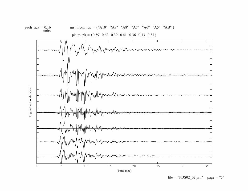
each_tick 0.16= inst_from_top "A10" "A9" "A8" "A7" "A6" "A5" "AB"( )=units

0 5 10 15 20 25 30 35Time (sec)

Lege

nd a

nd sc

ale

abov

epk_to_pk 0.59 0.62 0.39 0.41 0.36 0.33 0.37( )=



0 5 10 15 20 25 30 35Time (sec)

Lege

nd a

nd sc

ale

abov

epk_to_pk 0.42 0.41 0.35 0.38 0.37( )=


each_tick 0.05= inst_from_top "A14" "A13" "A12" "AB"( )=units

0 5 10 15 20 25 30 35Time (sec)

Lege

nd a

nd sc

ale

abov

epk_to_pk 0.13 0.22 0.22 0.37( )=



0 5 10 15 20 25 30 35Time (sec)

Lege

nd a

nd sc

ale

abov

epk_to_pk 982.90 647.61 383.51 858.89 1.58 103× 557.59( )=



0 5 10 15 20 25 30 35Time (sec)

Lege

nd a

nd sc

ale

abov

epk_to_pk 220.46 392.70 546.56 734.88 895.63 557.59( )=

file "PDS02_02.prn"= page "8a"=

each_tick 248.21= inst_from_top "NEA4" "NES3" "NES2" "NEA1" "AB"( )=units

0 5 10 15 20 25 30 35Time (sec)

Lege

nd a

nd sc

ale

abov

epk_to_pk 1.87 103× 331.62 555.22 1.55 103× 557.59( )=


each_tick 82.20= inst_from_top "CWA4" "CWS3" "CWS2" "AB"( )=units

0 5 10 15 20 25 30 35Time (sec)

Lege

nd a

nd sc

ale

abov

epk_to_pk 90.44 338.32 580.34 557.59( )=


each_tick 204.81= inst_from_top "CEM5" "CEM4" "CEM3" "CEM2" "AB"( )=units

0 5 10 15 20 25 30 35Time (sec)

Lege

nd a

nd sc

ale

abov

epk_to_pk 567.23 909.41 668.28 1.29 103× 557.59( )=


each_tick 322.90= inst_from_top "SWM7" "SWM6" "SWM5" "SWM4" "SWM3" "SWM2" "AB"( )=units

0 5 10 15 20 25 30 35Time (sec)

Lege

nd a

nd sc

ale

abov

epk_to_pk 969.12 845.11 505.23 617.76 1.11 103× 1.70 103× 557.59( )=


each_tick 170.16= inst_from_top "SWM12" "SWM11" "SWM10" "SWM9" "SWM8" "AB"( )=units

0 5 10 15 20 25 30 35Time (sec)

Lege

nd a

nd sc

ale

abov

epk_to_pk 140.09 413.37 583.31 718.80 861.18 557.59( )=

file "PDS02_02.prn"= page "12a=

each_tick 238.15= inst_from_top "SEA4" "SES3" "SES2" "SEA1" "AB"( )=units

0 5 10 15 20 25 30 35Time (sec)

Lege

nd a

nd sc

ale

abov

epk_to_pk 1.73 103× 352.56 649.84 1.37 103× 557.59( )=


each_tick 37.38= inst_from_top "L14" "L13" "L2" "L1" "AB"( )=units

0 5 10 15 20 25 30 35Time (sec)

Lege

nd a

nd sc

ale

abov

epk_to_pk 206.81 205.71 5.42 109.51 185.86( )=



0 5 10 15 20 25 30 35Time (sec)

Lege

nd a

nd sc

ale

abov

epk_to_pk 648.67 511.74 477.42 283.75 219.11 185.86( )=



0 5 10 15 20 25 30 35Time (sec)

Lege

nd a

nd sc

ale

abov

epk_to_pk 25.37 24.94 1.04 103× 90.71 61.29 185.86( )=


APPENDIX A:CENTER FOR GEOTECHNICAL MODELING March 2000

CENTER DIRECTORS:James A. Cheney 1983-1989I. M. Idriss 1989-1996Bruce L. Kutter 1996-

FACILITY MANAGEMENT:Bruce L. Kutter 1983-1990 Managing Director

1990-1996 Associate DirectorD. P. Stewart 1995-1997 Facility ManagerD. W. Wilson 1997- Facility Manager

DESCRIPTION OF CENTRIFUGE FACILITIES

9 m CENTRIFUGE AND SHAKER

In 1978, in response to a broad agency announcement from NSF, UC Davis collaboratedwith NASA to propose the development of a large geotechnical centrifuge facility. The proposalwas successful, and the centrifuge was constructed and installed at the NASA Ames ResearchCenter. The centrifuge was first operated at NASA Ames in early 1984. In 1987, NASAdisassembled the centrifuge and hauled it to UC Davis. Using funds from Tyndall AFB, LosAlamos National Laboratories, the National Science Foundation and the University of California,the centrifuge was installed and operated on a concrete slab in the open air in 1988; in thisconfiguration, the maximum acceleration that could be achieved was 19 g. NSF then funded theconstruction of an enclosure around the centrifuge, which was completed in December 1989 andallowed the centrifuge to achieve accelerations of 50 g. From 1990-1995, a large amount ofeffort was expended to raise funds, design, and develop an earthquake simulation capability forthe large centrifuge. The shaker development was supported by NSF, Caltrans, the ObayashiCorporation, and the University of California. In April 1995, the first proof tests of the shakerwere conducted at a centrifugal acceleration of 50 g. In 1996, the focus of the Center finallyshifted from facility development to utilization of the shaker and centrifuge facilities.

This centrifuge, in terms of radius (9.1 m to bucket floor), maximum payload mass(5000 kg), and available bucket area (4.0 m2) is one of the largest geotechnical centrifuges in theworld. At present, the centrifuge is limited to centrifugal accelerations up to 40 g. Thecentrifuge capacity in terms of the maximum acceleration multiplied by the maximum payload is40 g x 5000 kg = 200 g-tonnes.

The data acquisition system on the centrifuge is kept up to date by continual upgrades tothe data acquisition systems. Low level signals are conditioned with instrumentation amplifiersat the end of the centrifuge arm. Commercially available programmable gain, programmablecutoff frequency anti-aliasing amplifiers mounted at the center of the centrifuge are used prior todigitization. At present the system has a capability to digitize over 100 channels of data at about2000 samples per second per channel. The digitization takes place onboard the centrifuge by acommercial data acquisition board (Data Translations DT2839) installed in a standard personalcomputer. The data is stored on a conventional hard disk on the centrifuge computer and then

transmitted to another computer in the control room via an Ethernet network and remote controlsoftware.

Some specifications of the large servo-hydraulic shaker are summarized here; a moredetailed description is given by Kutter et al. (1994). For a rigid shaking mass of 2700 kg (modelplus container), the actuators, operating with 3500 psi (24 MPa) oil pressure theoretically havethe capacity to produce 14 g shaking accelerations at frequencies up to 200 Hz. In practice, muchlarger accelerations (up to 40 g) can be obtained because the models do not behave like a rigidmass at high frequencies. The maximum absolute shaking velocity is about 1 m/s and the strokeis 2.5 cm peak to peak. To achieve this, two pairs of single acting actuators provide a net peakactuator force of 400 kN. One actuator pair is mounted on each side of the model container.Each actuator pair (patented by Team Corporation) consists of two-single-acting actuators boltedon opposite sides of a two-stage servo-valve block.

The actuators are controlled by a conventional closed loop feedback control system. Asimple correction scheme is used to precondition the command signal to improve the coherenceand frequency content of the shaking table motions. In addition to step waves, sine waves andsine sweeps, simulations of ground motions recorded in a number of different earthquakes havebeen produced in the shaker.

Two flexible shear beam containers (FSB1, and FSB2) and a rigid container withwindows (RC1) are available. FSB2 and RC1 have dimensions of approximately1.7 x 0.8 x 0.5 m (Length by Width by Height), with the shaking in the direction of the length.FSB1 has dimensions of about 1.7 x 0.7 x 0.6 m. The FSB containers consist of a stack ofrectangular rings of aluminum tubing and rubber. The rubber is flexible in shear, which allowsthe container to deform with the soil. The stiffness of the rubber is designed to make the naturalfrequency of the container (as a shear beam) to be less than the natural frequency of a soil layer.

In the Fall of 2000, UC Davis received a $4.6 million grant from the National ScienceFoundation (NSF), as a part of the Network for Earthquake Engineering Simulation (NEES)program, to upgrade and enhance the large centrifuge and become a NEES host facility. Theupgrades include an in-flight robot, new sensor equipment, modifications to allow operations upto 80-g, a new hinged-plate container, a biaxial horizontal/vertical shaker, tele-observation andtele-operation capabilities, data visualization capabilities, and in-flight tomographic imaging andgeophysical tools. These upgrades will be operational in 2004.www.eng.nsf.gov/nees/default.htm

SCHAEVITZ CENTRIFUGE AND SHAKER

The 1 m radius centrifuge can carry 90 kg models to 100 g or 27 kg models to 175 g. Thecentrifuge is equipped with a servo-hydraulic actuator which is capable of simulating earthquake-like motions to the base of the model container during flight. The shaker has been used to studythe dynamic behavior of retaining structures, liquefiable soil layers, response of soft soil sites,soil-pile-structure interaction, flow slides, embankments and port structures. Over a thousandmodel earthquakes have been produced by this shaker, and it was the primary focus of thecentrifuge modeling efforts of the faculty at UCD until completion of the large shaker in 1995.

The shaker on the 1 m centrifuge has a model container with dimensions 0.56 x 0.28 x0.18 m. The shaker, capable of producing 30 g shaking accelerations is designed to operate atcentrifuge accelerations up to 100 g. A computer outside the centrifuge is used to control theshaker and to acquire data from the experiment. Sixteen channels of data can be digitized at ratesup to 2500 samples per second per channel. Sixteen variable gain amplifiers for strain gage type

instruments and eight variable gain charge amplifiers for accelerometers are mounted on thecentrifuge to improve the signal to noise ratio.

This centrifuge is equipped with four hydraulic rotary joints which may be used forhydraulic oil, water supply, or compressed gas. On board accumulators store energy incompressed gas to provide the short burst of high power required to produce large flow rates ofhigh pressure oil to for the shaker. The hydraulic system has also been used to apply static loadsto foundations and other mechanisms on the centrifuge.

FURTHER INFORMATION

Anyone interested in using or collaborating in the use of the centrifuge facilities is encouraged tocontact:

Bruce L. Kutter, Director, Center for Geotechnical ModelingDepartment of Civil and Environmental EngineeringUniversity of CaliforniaDavis CA 95616Tel: 916 752 8099Fax: 916 752 7872email: [email protected]

REFERENCES

Kutter, B.L., Li, X.S., Sluis, W., and Cheney, J.A. (1991) "Performance and Instrumentation ofthe Large Centrifuge at UC Davis", Centrifuge 91, Ko and McLean (eds.), Balkema, Rotterdam.

Kutter, B.L., Idriss, I.M., Kohnke, T., Lakeland, J., Li, X.S., Sluis, W., Zeng, X., Tauscher, R.C.,Goto, Y. Kubodera, I., (1994) "Design of a Large Earthquake Simulator at UC Davis, Centrifuge94, Leung, Lee, and Tan (eds.), Balkema, Rotterdam, pp. 169-175.

BEHAVIOR OF PILES IN LATERALLY SPREADING GROUND DURING EARTHQUAKES - REPORT FOR PDS02

Documents

Transcript of BEHAVIOR OF PILES IN LATERALLY SPREADING GROUND DURING EARTHQUAKES - REPORT FOR PDS02