FINITE ELEMENT MODELING OF AN INFLATABLE WING
149
University of Kentucky University of Kentucky UKnowledge UKnowledge University of Kentucky Master's Theses Graduate School 2007 FINITE ELEMENT MODELING OF AN INFLATABLE WING FINITE ELEMENT MODELING OF AN INFLATABLE WING Johnathan Rowe University of Kentucky, [email protected] Right click to open a feedback form in a new tab to let us know how this document benefits you. Right click to open a feedback form in a new tab to let us know how this document benefits you. Recommended Citation Recommended Citation Rowe, Johnathan, "FINITE ELEMENT MODELING OF AN INFLATABLE WING" (2007). University of Kentucky Master's Theses. 475. https://uknowledge.uky.edu/gradschool_theses/475 This Thesis is brought to you for free and open access by the Graduate School at UKnowledge. It has been accepted for inclusion in University of Kentucky Master's Theses by an authorized administrator of UKnowledge. For more information, please contact [email protected].
-
Upload
khangminh22 -
Category
Documents
-
view
4 -
download
0
Transcript of FINITE ELEMENT MODELING OF AN INFLATABLE WING

University of Kentucky University of Kentucky
UKnowledge UKnowledge
University of Kentucky Master's Theses Graduate School
2007
FINITE ELEMENT MODELING OF AN INFLATABLE WING FINITE ELEMENT MODELING OF AN INFLATABLE WING
Johnathan Rowe University of Kentucky, [email protected]
Right click to open a feedback form in a new tab to let us know how this document benefits you. Right click to open a feedback form in a new tab to let us know how this document benefits you.
Recommended Citation Recommended Citation Rowe, Johnathan, "FINITE ELEMENT MODELING OF AN INFLATABLE WING" (2007). University of Kentucky Master's Theses. 475. https://uknowledge.uky.edu/gradschool_theses/475
This Thesis is brought to you for free and open access by the Graduate School at UKnowledge. It has been accepted for inclusion in University of Kentucky Master's Theses by an authorized administrator of UKnowledge. For more information, please contact [email protected].

ABSTRACT OF THESIS
FINITE ELEMENT MODELING OF AN INFLATABLE WING
Inflatable wings provide an innovative solution to unmanned aerial vehicles requiring small packed volumes, such as those used for military reconnaissance or extra-planetary exploration. There is desire to implement warping actuation forces to change the shape of the wing during flight to allow for greater control of the aircraft. In order to quickly and effectively analyze the effects of wing warping strategies on an inflatable wing, a finite element model is desired. Development of a finite element model which includes woven fabric material properties, internal pressure loading, and external wing loading is presented. Testing was performed to determine material properties of the woven fabric, and to determine wing response to static loadings. The modeling process was validated through comparison of simplified inflatable cylinder models to experimental test data. Wing model response was compared to experimental response, and modeling changes including varying material property models and mesh density studies are presented, along with qualitative wing warping simulations. Finally, experimental and finite element modal analyses were conducted, and comparisons of natural frequencies and mode shapes are presented.
KEYWORDS: Finite Elements, Inflatable Wings, Unmanned Aerial Vehicle, Modal
Analysis, Internal Pressurization
Johnathan Rowe
August 7, 2007

FINITE ELEMENT MODELING OF AN INFLATABLE WING
By
Johnathan Michael Rowe
Dr. Suzanne Weaver Smith Director of Thesis
Dr. L. Scott Stephens
Director of Graduate Studies August 7, 2007

RULES FOR THE USE OF THESES
Unpublished theses submitted for the Master’s degree and deposited in the University of Kentucky Library are as a rule open for inspection, but are to be used only with due regard to the rights of the authors. Bibliographical references may be noted, but quotations or summaries of parts may be published only with the permission of the author, and with the usual scholarly acknowledgments. Extensive copying of publication of the thesis in whole or in part also requires the consent of the Dean of the Graduate School of the University of Kentucky. A library that borrows this thesis for use by its patrons is expected to secure the signature of each user. Name Date ________________________________________________________________________ ________________________________________________________________________ ________________________________________________________________________ ________________________________________________________________________ ________________________________________________________________________ ________________________________________________________________________ ________________________________________________________________________ ________________________________________________________________________ ________________________________________________________________________ ________________________________________________________________________ ________________________________________________________________________ ________________________________________________________________________ ________________________________________________________________________

THESIS
Johnathan Michael Rowe
The Graduate School
University of Kentucky
2007

FINITE ELEMENT MODELING OF AN INFLATABLE WING
_________________________________
THESIS __________________________________
A thesis submitted in partial fulfillment of the
requirements for the degree of Master of Science in the College of Engineering at the
University of Kentucky
By
Johnathan Michael Rowe
Lexington, Kentucky
Director: Dr. Suzanne Weaver Smith, Associate Professor of Mechanical Engineering
Lexington, Kentucky
2007

ACKNOWLEDGMENTS
I would like to thank my advisor Dr. Suzanne Smith for offering me such a
challenging research project, and for offering guidance and insight throughout the course
of my research. Through her role as my advisor she has helped me grow substantially as
an engineer over the past few years.
The author would like to acknowledge Stephen Scarborough and Matt MacKusick at
ILC Dover for performing experimental testing of the Vectran material and providing the
data from those experiments. Thanks go to David Miller for performing additional
experimental tests on the wings.
Former co-worker Dr. Jonathan Black must be acknowledged for his help in
performing the experimental modal analysis and performing modal parameter estimation
using the X-Modal software. Thanks to Andrew Simpson for his general knowledge of
the wings, his help with performing experimental testing, and the use of his discount card
for free drinks at Jimmy Johns.
Funding for this research was provided by a grant from The Kentucky Science and
Engineering Foundation and also by fellowships from the Kentucky Space Grant
Consortium and the Center for Computational Sciences at the University of Kentucky.
I must thank my parents, Kenzie and Beverly Rowe for their love and support
throughout both my undergraduate and graduate careers, without which I would not be
where I am today.
Finally, thanks must be given to The Crystal Method for recording Vegas, which
served as excellent background music during the writing of this thesis.
iii

TABLE OF CONTENTS
ACKNOWLEDGMENTS .......................................................................................................................III
TABLE OF CONTENTS ....................................................................................................................... IV
LIST OF TABLES................................................................................................................................. VII
LIST OF FIGURES..............................................................................................................................VIII
CHAPTER 1: INTRODUCTION..............................................................................................................1
1.1 MOTIVATION ...................................................................................................................................2
1.2 OBJECTIVES .....................................................................................................................................3
1.3 OVERVIEW OF THESIS ......................................................................................................................4
CHAPTER 2: BACKGROUND................................................................................................................5
2.1 EARLY INFLATABLE WING TECHNOLOGY........................................................................................5
2.2 RECENT DEVELOPMENTS IN INFLATABLE WING TECHNOLOGY .......................................................7
2.3 MORPHING INFLATABLE WINGS ....................................................................................................12
2.4 PREVIOUS ANALYTICAL MODELING OF INFLATABLE STRUCTURES ...............................................13
2.5 PREVIOUS MODELING OF INFLATABLE STRUCTURES USING FINITE ELEMENTS .............................15
2.6 PREVIOUS EXPERIMENTAL TESTING OF INFLATABLE STRUCTURES ...............................................16
2.7 DESCRIPTION OF TEST ARTICLE.....................................................................................................16
CHAPTER 3: STATIC EXPERIMENTAL TESTING...........................................................................20
3.1 TENSILE TESTING OF VECTRAN STRIPS...........................................................................................20
3.2 SHEAR TESTING OF INFLATABLE CYLINDERS ................................................................................21
3.3 PRELIMINARY STATIC BENDING TESTS..........................................................................................24
3.3.1 Experimental Set-up ..............................................................................................................24
3.3.2 Wing Stiffness Calculations...................................................................................................28
3.4 REVISED WING BENDING TESTS ....................................................................................................29
3.5 WING TWIST TESTS .......................................................................................................................36
iv

3.5.1 Experimental Results.............................................................................................................36
3.5.2 Wing Torsional Stiffness Calculations ..................................................................................40
CHAPTER 4: FINITE ELEMENT MODELING OF STATIC LOAD CASES .....................................42
4.1 FE ANALYSIS OF SHEAR TEST CYLINDERS ....................................................................................43
4.2 FE MODEL OF INFLATABLE WINGS................................................................................................48
4.2.1 FE Model Geometry..............................................................................................................48
4.2.2 Mesh Convergence................................................................................................................50
4.2.3 Material Models ....................................................................................................................51
4.2.4 Application of Loads .............................................................................................................53
4.3 FE SIMULATIONS OF STATIC LOADS ..............................................................................................54
4.3.1 Wing Bending........................................................................................................................54
4.3.2 Wing Twist.............................................................................................................................61
4.4 SIMULATION OF WING WARPING...................................................................................................64
CHAPTER 5: EXPERIMENTAL AND FE MODAL ANALYSES.......................................................71
5.1 EXPERIMENTAL MODAL ANALYSIS ...............................................................................................71
5.1.1 Test Setup ..............................................................................................................................71
5.1.2 Signal Processing and Typical Results .................................................................................75
5.1.3 Modal Parameter Identification............................................................................................79
5.2 FE MODAL ANALYSIS....................................................................................................................84
5.2.1 Model Description and Solution Process..............................................................................84
5.2.2 Linear Pressurization Results ...............................................................................................85
5.2.3 Nonlinear Pressurization Results..........................................................................................86
CHAPTER 6: SUMMARY .....................................................................................................................91
6.1 DETAILED SUMMARY.....................................................................................................................91
6.2 CONTRIBUTIONS ............................................................................................................................93
6.3 FUTURE WORK ..............................................................................................................................93
v

APPENDIX A: ANSYS BATCH FILE COMMANDS ..........................................................................95
APPENDIX B: ADDITIONAL EXPERIMENTAL TEST DATA.......................................................119
REFERENCES ......................................................................................................................................131
VITA .....................................................................................................................................................135
vi

LIST OF TABLES
Table 3.1 – Initial Young’s moduli determined from tensile testing of urethane coated Vectran. ................21
Table 3.2 – Experimentally determined values of shear moduli of urethane-coated Vectran .......................24
Table 4.1 – Vectran material properties used in the cylinder model .............................................................44
Table 4.2 – Initial material properties used in FE model ..............................................................................52
Table 4.3 – Loadings applied for each wing warping analysis......................................................................66
Table 5.1 - Natural frequencies and mode shapes seen in frequency range, 15 psi internal pressure ...........80
Table 5.2 – Estimated wing damped natural frequencies and damping ........................................................83
Table 5.3 – Wing undamped natural frequencies and damping ....................................................................83
Table 5.4 – FE predictions of wing natural frequencies, linear pressure solution.........................................86
Table 5.5 – Percent error from experimental in linearly applied pressure FE resonant frequencies .............86
Table 5.6 – FE predictions of wing modes and natural frequencies calculated using non-linear pressure
solution, linear orthotropic material model..........................................................................................89
Table 5.7 – FE predictions of wing modes and natural frequencies calculated using, non-linear pressure
solution, nonlinear isotropic material model........................................................................................89
vii
LIST OF FIGURES
Figure 1.1 – Conceptual configuration of a Mars glider employing inflatable wings .....................................2
Figure 2.1 – Model GA-468 Goodyear Inflatoplane .......................................................................................6
Figure 2.2 – Apteron R/C UAV designed by ILC Dover [17] ........................................................................6
Figure 2.3 – Deployment and inflation sequence of NASA Dryden's I-2000 UAV........................................8
Figure 2.4 – BIG BLUE II glider after recovery with rigidized wings............................................................9
Figure 2.5 – High-altitude deployment of inflatable wing, April 30, 2005 ...................................................10
Figure 2.6 – AIRCAT UAV with inflatable wings........................................................................................11
Figure 2.7 – BIG BLUE V glider, just before high-altitude launch. .............................................................12
Figure 2.8 – Low pressure inflatable wings with attached warping mechanism. ..........................................13
Figure 2.9 – In-flight photo of inflatable wing aircraft with servo actuated wing warping...........................13
Figure 2.10 – Close up view of wing tip. ......................................................................................................17
Figure 2.11 – Inflatable wing components. (Image provided by ILC Dover) ...............................................18
Figure 2.12 – Inflatable wings in packed and deployed configurations. (Image provided by ILC Dover) ...19
Figure 2.13 – Wing dimensions. (Image provided by ILC Dover)................................................................19
Figure 3.1 – Uninflated shear test cylinder and shear test setup. (Images provided by ILC Dover) .............22
Figure 3.2 – Shear stress-strain diagram for cylinder with longitudinal warp...............................................23
Figure 3.3 – Shear stress-strain diagram for cylinder with hoop warp..........................................................24
Figure 3.4 – Measurement points for initial bending test ..............................................................................25
Figure 3.5 – Wing bending test set-up...........................................................................................................26
Figure 3.6 – Inflatable wing tip deflection results.........................................................................................26
Figure 3.7 – Flexural rigidity of wing. ..........................................................................................................29
Figure 3.8 – Bending test set-up....................................................................................................................30
Figure 3.9 – Vertical wing deflections, 15 psig internal pressure. ................................................................32
Figure 3.10 – Vertical deflection at wing tip after applying and removing 11.24 lbf loading.......................32
Figure 3.11 – Wing deflections, 4.5 lbf tip load over a range of internal pressures ......................................34
Figure 3.12 – Comparison between bending tests, deflections at wing tip shown. .......................................35
Figure 3.13 – Average vertical wing tip deflections and standard deviations of inflatable wings ................36
viii

Figure 3.14 – Wing under 7.01 lb couple forces for twist loading and 25 psig internal pressure. ................37
Figure 3.15 – Wing deflections, 15 psig internal pressure. ...........................................................................38
Figure 3.16 – Wing deflections, 82.4 lb-in applied torque. ...........................................................................39
Figure 3.17 – Angle of twist of wing for 82.4 lb-in applied torque...............................................................39
Figure 3.18 – Torsional rigidity of wing for 10 psig internal pressure..........................................................41
Figure 3.19 – Torsional rigidity of wing for 82.3 lb-in torque applied at wing tip........................................41
Figure 4.1 – FE model of inflatable test cylinders with coarse (left) and fine (right) meshes.......................44
Figure 4.2 – Comparison of results from cylinder with longitudinal warp, 1 psi internal pressure...............45
Figure 4.3 – Comparison of results from cylinder with hoop warp, 1 psi internal pressure..........................46
Figure 4.4 – Wing dimensions in inches .......................................................................................................49
Figure 4.5 – Meshed inflatable wing model ..................................................................................................50
Figure 4.6 – Mesh densities...........................................................................................................................51
Figure 4.7 – Tensile test stress-strain diagrams for both material directions. ...............................................53
Figure 4.8 – Material model used in the FE model. ......................................................................................53
Figure 4.9 – Comparison of experimental and FE wing deflection results ...................................................56
Figure 4.10 – Comparison of experimental and FE wing deflection results..................................................57
Figure 4.11 – Deflected wing shape for 15-psi pressurization and 11.2-lbf tip load.....................................58
Figure 4.12 – Comparison of experimental and FE wing bending results for 10 psi, deflection at wing tip
shown...................................................................................................................................................60
Figure 4.13 – Comparison of experimental and FE wing bending results for 15 psi, deflection at wing tip
shown...................................................................................................................................................60
Figure 4.14 – Comparison of angle of twist at wing tip, negative twist applied. ..........................................62
Figure 4.15 – Deflected wing shape for 15-psi pressurization and 82.4-lb-in tip load..................................63
Figure 4.16 – Comparison of experimental and FE angle of twist at wing tip due to applied torques ..........64
Figure 4.17 – Locations of applied moments on underside of wing..............................................................66
Figure 4.18 – Analysis 1 resulting deflections. Scale increased by 5X.........................................................68
Figure 4.19 – Analysis 2 resulting deflections. Scale increased by 5X.........................................................68
Figure 4.20 – Analysis 3 resulting deflections. Scale increased by 5X.........................................................69
ix

Figure 4.21 – Predicted wing deflections vs. number of servos ....................................................................69
Figure 4.22 – Analysis 4 resulting deflections. Scale increased by 5X.........................................................70
Figure 4.23 – Analysis 5 resulting deflections. Scale increased by 5X.........................................................70
Figure 5.1 – Block diagram of experimental test setup .................................................................................72
Figure 5.2 – Photo of test setup showing placement of accelerometers ........................................................73
Figure 5.3 – Locations of excitation test points on the wing. Note that excitation points 9 and 10 are also
measurement locations of accelerometers............................................................................................73
Figure 5.4 – FRFs of wing at both measurement points due to excitation at point 4, with wing internal
pressure of 15 psi .................................................................................................................................75
Figure 5.5 – FRF plots comparing 10 and 30 average tests, 20 psig, Sensor 1 .............................................76
Figure 5.6 – FRF plots comparing 10 and 30 average tests, 20 psig, Sensor 1 .............................................76
Figure 5.7 – FRF plots demonstrating reciprocity, 5 psig .............................................................................78
Figure 5.8 – FRF plots demonstrating reciprocity, 25 psig ...........................................................................78
Figure 5.9 – Consistency diagram for modal testing using PTD method......................................................79
Figure 5.10 – Residue results for the FRF at measurement Point 9 and excitation Point 3...........................82
Figure 5.11 – Experimentally determined mode shapes, 15 psig internal pressure.......................................82
Figure 5.12 – Comparison between estimated wing natural frequencies from experimental modal testing
and predicted natural frequencies from FE modal analysis with linear pressurization solution ..........86
Figure 5.13 – FE predicted mode shapes using adjusted nonlinear isotropic material model and mesh
density of 69,750 DOF.........................................................................................................................90
x

CHAPTER 1: INTRODUCTION
An Unmanned Aerial Vehicle (UAV) is any aircraft that does not have a pilot
onboard. Instead, UAV’s are controlled from a remote location through the use of radio-
control (RC), or by an onboard autopilot system. The most common uses of UAV’s are
by the military for surveillance or reconnaissance missions. Use of UAV’s has the benefit
of allowing missions to be completed without risking human lives. In addition, by
removing the pilot element from the overall flight mission equation, UAV’s allow for
more freedom in mission objectives, such as the ability to lengthen flight times. Also,
UAV’s have the potential to be less expensive than standard aircraft, as no
accommodations are needed for an onboard pilot, for example, lesser environmental or
atmospheric accommodations are needed for high-altitude flight. UAV sizes range from
very large to micro [1]. The focus of this thesis is on the class of small (~ 6 ft wingspan)
UAVs.
In addition to military uses, another application that a UAV is especially well suited
for is extra-planetary exploration, most specifically Mars. A Mars airplane would allow
for a more detailed view of the planet’s surface than a satellite, yet can cover a larger area
than a rover. One major challenge in deployment of a Mars glider is the problem of
getting such an aircraft to Mars to be deployed. The concept of inflatable wings provides
a unique solution to the problem of stowing an aircraft in a small volume. The wings can
be packed in a deflated state in a volume many times smaller than the final deployed
volume of the wings, and then once the aircraft is released from the launch vehicle, the
1
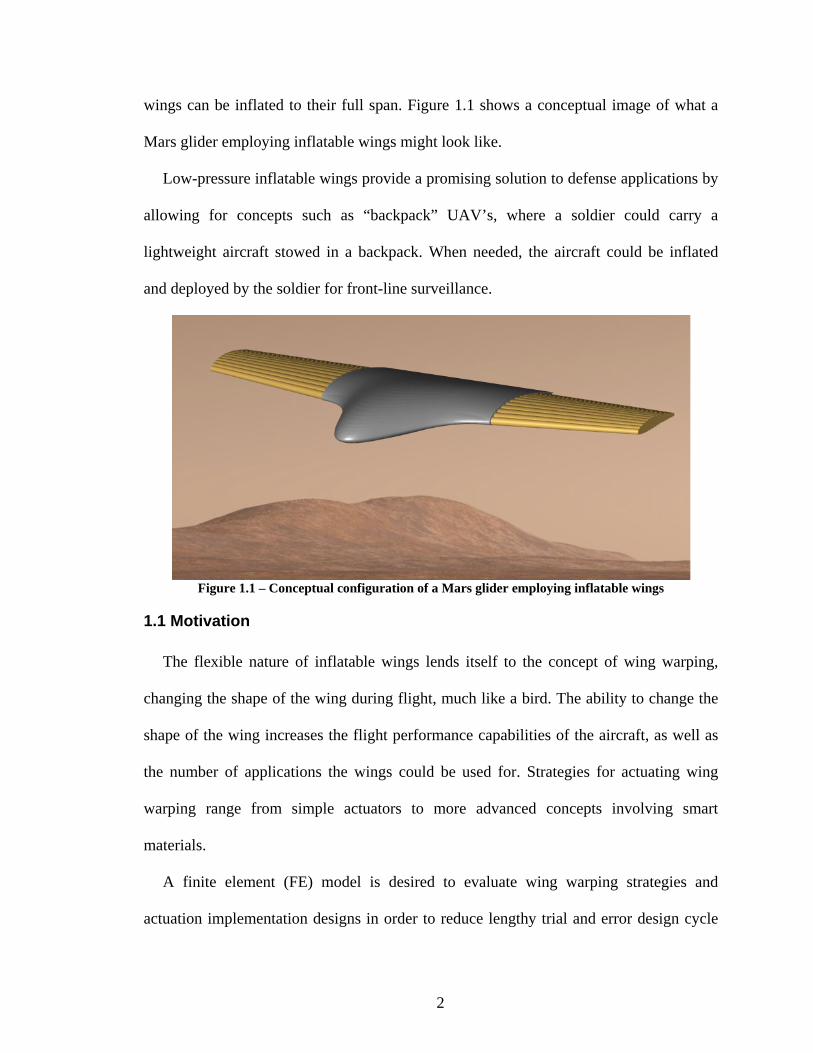
wings can be inflated to their full span. Figure 1.1 shows a conceptual image of what a
Mars glider employing inflatable wings might look like.
Low-pressure inflatable wings provide a promising solution to defense applications by
allowing for concepts such as “backpack” UAV’s, where a soldier could carry a
lightweight aircraft stowed in a backpack. When needed, the aircraft could be inflated
and deployed by the soldier for front-line surveillance.
Figure 1.1 – Conceptual configuration of a Mars glider employing inflatable wings
1.1 Motivation
The flexible nature of inflatable wings lends itself to the concept of wing warping,
changing the shape of the wing during flight, much like a bird. The ability to change the
shape of the wing increases the flight performance capabilities of the aircraft, as well as
the number of applications the wings could be used for. Strategies for actuating wing
warping range from simple actuators to more advanced concepts involving smart
materials.
A finite element (FE) model is desired to evaluate wing warping strategies and
actuation implementation designs in order to reduce lengthy trial and error design cycle
2

times. Ultimately, the interest in the development of a finite element model of inflatable
wings lies in the desire for the ability to predict responses of the wings to combined-
loading situations including applied aerodynamic loads from wind tunnel or actual flight
testing and forces applied to change the shape of the wings. Of course in order to predict
unknown responses, the model of such a complex structural system must first be
validated through comparisons of results from FE analyses and experiments, which is
where the majority of the focus of this thesis lies. For this complex system, phased
validation is necessary, ranging from material properties and simpler pressurization
models, to static response to external loads, and finally to dynamic response.
1.2 Objectives
Therefore, the objectives for this research are outlined as follows:
• Determine the response of an inflatable wing.
o Investigate the material properties of Vectran.
o Perform experimental tests on the wing to determine static response to
bending and torsion loads.
o Determine dynamic characteristics of the wing through an experimental
modal analysis.
• Develop a FE model that can be used to predict wing response.
o Combine methods previously used to model inflatable structures and
morphing inflatable wings.
o Validate the model through comparison of FE simulations and
experimental results.
o Use the FE model to predict responses to wing warping loads.
3

1.3 Overview of Thesis
In this thesis, Chapter 2 provides a literature review of previous work on inflatable
wings, as well as previous attempts to model inflatable structures, using both analytical
and FE methods. Material property testing performed by the wing manufacturer is
discussed in Chapter 3, along with static testing performed on the wing for this research.
Chapter 4 discusses the FE modeling process of the inflatable wing, as well as FE
simulations to static load cases. Chapter 5 gives a description of experimental modal
testing performed on the wing, as well as FE predictions of the natural frequencies and
mode shapes of the wing. Finally, Chapter 6 presents a summary of the work contained
herein as well as possibilities for future work.
4

CHAPTER 2: BACKGROUND
Inflatable structures provide unique solutions for designs requiring small packed
volumes. The concept of inflatable wings was developed decades ago, but a new cycle of
research and innovation is underway. New missions are being considered, requiring
unique packaging solutions and employing new materials to address previous concerns.
Inflatable wing technology is being studied as an alternative for small UAVs providing
packaging advantages and opportunities for wing warping or morphing [2-5].
Development of morphing technology for inflatable wings is of interest because it allows
for adjustments to be made to the profile of the wing during flight, thus enlarging the
flight envelope for the aircraft. New materials address previous concerns about punctures
and deflation. Wings can be constructed of rigidizable fabric composites that harden after
deployment and exposure to UV radiation or of rugged woven materials to prevent
damage [6-9]. Inflatable wing technology is also being studied as a feasible option for
extra-planetary exploration, particularly for Mars [10, 11]. To date, four successful high-
altitude balloon experiments have demonstrated deployment of inflatable wings at low
density, low temperature conditions [12-15].
2.1 Early Inflatable Wing Technology
An early example of inflatable aircraft technology is the Goodyear Inflatoplane.
Goodyear Aircraft Company designed and built this aircraft as a plane that could be
dropped uninflated from an aircraft to downed pilots behind enemy lines. The pilot could
then inflate the plane and use it to escape. The aircraft was able to be inflated using less
pressure than a car tire in approximately five minutes. The project began in 1956 and was
5

finally cancelled in 1973. Twelve Inflatoplanes were built during the course of the project
[16].
Figure 2.1 – Model GA-468 Goodyear Inflatoplane
Inflatable wings were developed for an unmanned aircraft in the 1970’s by ILC Dover
with the Apteron R/C plane shown in Figure 2.2. The wingspan of the Apteron was 5.1 ft,
and the aircraft had a total weight of 7 lbs. Propulsion was provided by a 0.5 HP engine,
and elevons provided control.
Figure 2.2 – Apteron R/C UAV designed by ILC Dover [17]
6

2.2 Recent Developments in Inflatable Wing Technology
ILC Dover has more recently resumed efforts on inflatable wing technology, and has
developed many inflatable and inflatable/rigidizable wings which have been documented
extensively elsewhere [5, 8, 9, 12-14, 18-20]. Inflation pressures are generally low,
ranging from 7 to 27 psig. ILC Dover is the manufacturer of the wings considered in this
thesis.
In 2001, NASA Dryden successfully demonstrated in-flight deployment of an
inflatable wing aircraft followed by a successful low-altitude glide. The I-2000 UAV
employed wings developed by Vertigo Inc. for use by the U.S. Navy. The wings were
constructed of cylindrical, inflatable spanwise spars that ran from wingtip to wingtip,
with a wingspan of 64 in. and a chord length of 7.25 in [4]. The wings were designed for
inflation pressures ranging from 150 psi to 300 psi. Figure 2.3 shows the release and
inflation sequence of the UAV.
7

Figure 2.3 – Deployment and inflation sequence of NASA Dryden's I-2000 UAV
Work has been done at the University of Kentucky to verify the feasibility of
inflatable wing technology for use on a planetary scout aircraft; most notably, an
inflatable wing “scout” glider for Mars exploration. The BIG BLUE project (Baseline
Inflatable-wing Glider Balloon Launched Unmanned Experiment) is an undergraduate
program at the University of Kentucky in which high-altitude tests are conducted by
sending inflatable wings to roughly 100,000 ft on weather balloons. At this altitude, the
atmospheric density is similar to that seen at flight level on Mars. Each year, a new group
of students participated in the project, with a high-altitude balloon launch or other major
flight test being the final goal each Spring. To date, there have been five BIG BLUE
mission groups, with four of those culminating in high-altitude balloon launches, each
increasing in complexity toward a final high-altitude flight mission. For the final mission,
8

the end goal was to inflate the wings during ascent, allow the wings to cure, and then
when the balloon reached critical altitude , the gliders would fly back to a designated
landing location [12, 15].
The first two years of the BIG BLUE project proved the feasibility of inflatable/UV-
rigidizable wings. The BIG BLUE I balloon launch marked the first time that this
technology had been demonstrated. The wings considered in these projects were designed
by the University of Kentucky in conjunction with ILC Dover, and contained a UV-
curable resin so that after the wings were inflated, internal pressurization was only
required for approximately 20 minutes while the resin cured and the wings became rigid.
Figure 2.4 – BIG BLUE II glider after recovery with rigidized wings
9

Beginning with BIG BLUE 3 in 2005, the focus of the project moved from
inflatable/rigidizable to purely inflatable wing technology. BIG BLUE 3 culminated with
a successful high-altitude balloon launch with the sole purpose of testing the design of an
inflation system to inflate the wings at high-altitude, and maintain pressure as the wings
returned to earth under a parachute. The wings considered during this project – the same
wings that are the focus of the research in the later chapters of this thesis – are described
in Section 2.7. Figure 2.5 shows the deployment of the wing at an altitude of
approximately 98,000 ft [13]. The following year, BIG BLUE 4 did not culminate in a
high altitude balloon launch as previous years had. The focus that year was to take the
successes of the previous year and develop an unmanned aerial vehicle utilizing inflatable
wings. The AIRCAT UAV with inflatable wings is shown in Figure 2.6.
Figure 2.5 – High-altitude deployment of inflatable wing, April 30, 2005
10
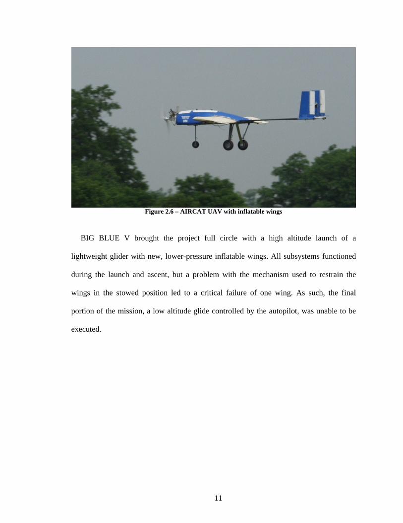
Figure 2.6 – AIRCAT UAV with inflatable wings
BIG BLUE V brought the project full circle with a high altitude launch of a
lightweight glider with new, lower-pressure inflatable wings. All subsystems functioned
during the launch and ascent, but a problem with the mechanism used to restrain the
wings in the stowed position led to a critical failure of one wing. As such, the final
portion of the mission, a low altitude glide controlled by the autopilot, was unable to be
executed.
11

Figure 2.7 – BIG BLUE V glider, just before high-altitude launch.
2.3 Morphing Inflatable Wings
Extensive research has been conducted at the University of Kentucky by Jacob and
Simpson on developing UAV’s with inflatable wings and varying methods of wing
warping [2, 3, 6, 7, 19-28]. An effective summary of this testing will be presented in
Simpson’s PhD Dissertation, published in 2007 [29].
An inflatable wing constructed of urethane coated nylon is shown in Figure 2.8 with
an early method of actuating warping for roll control. This wing, manufactured by ILC
Dover, is currently undergoing testing at the University of Kentucky to explore warping
capabilities and flight performance as shown in Figure 2.9.
12

Figure 2.8 – Low pressure inflatable wings with attached warping mechanism.
Figure 2.9 – In-flight photo of inflatable wing aircraft with servo actuated wing warping.
2.4 Previous Analytical Modeling of Inflatable Structures
Some understanding of response of inflatable wings can be gained through analytical
models and experimental studies of static loading and deployment response of inflated
cylinders and of spacecraft structures composed of inflated cylinders [30-33]. Main et al.
developed an analytical model for inflatable cylinder beam bending which closely
correlated to experimental testing [31]. This model expanded on previous work by
13
accounting for the beam fabric’s biaxial stress state, and its effect on the onset of
wrinkling. The model also accounts for the bending behavior of the beam after wrinkling
has occurred.
Analytical models for the response of inflated cylinders have been developed for the
prediction of static and dynamic response of inflating beams and for aeroelastic response
of inflatable wings for UAVs [34, 35]. Analytical modeling approaches have also been
applied to inflatable torus structures [36].
Researchers at NASA Dryden developed an analytical prediction of beam bending as a
supplemental effort to the I-2000 UAV [4]. In order to validate this analytical model,
comparisons to experimental testing were performed. This experimental testing showed
that over the range of pressures tested (150-300 psig) the initial slope of the load-
deflection curve was equivalent until the onset of wrinkling. In effect, it was seen that the
benefit of higher wing pressure is to expand the pre-wrinkle load range. The analytical
models developed correlated well to the experimental bending results, though other types
of loading were not considered. A finite element approach was also considered, but
results were not presented.
In Griffith’s Master’s thesis, work is presented on an experimental modal analysis of
an inflatable torus, as well as analytical methods to predict natural frequencies and mode
shapes [36]. One method of estimating natural frequencies considered by Griffith was the
use of circular ring models including bulk properties for the inflated system. It was found
that a finite element approach incorporating shell elements and prestress effects from
internal pressure loading was more accurate than using the analytical ring models. In
order to develop an accurate circular ring model, the frequency-dependent dynamic
14
modulus of the structure is needed, thus limiting the usefulness of this method as a pre-
test model.
2.5 Previous Modeling of Inflatable Structures using Finite Elements
FE models of inflatable/rigidizable wings were created previously by Usui as part of
the design effort for the wings used in the BIG BLUE II project at the University of
Kentucky [15]. The wings considered in this analysis contained a resin that would harden
the wings when exposed to UV radiation. Once the wings were rigidized, internal
pressure was no longer required. As the rigidized state was the flight state of these wings,
the FE models included material properties of the rigidized wings and did not include
internal wing pressures. These models included external aerodynamic loading as
distributed loads with appropriate spanwise and chordwise profiles. The wing models
developed by Usui are similar in concept to those considered in the later chapters of this
thesis. The FE modeling work done by Usui was an important reference for the work
contained in this thesis, and the general idea was to take the methodology used by Usui
and expand it to model wings that required internal pressurization to maintain their shape.
Previous FE modeling of an inflatable structure which includes internal pressurization
was performed by Griffith at the University of Kentucky.[36] FE modal analyses of an
inflatable Kapton torus were performed with natural frequencies and mode shapes being
correlated to experimental results. Two FE models were created for this purpose, one
modeling the torus with beam elements and using bulk properties for the inflated system,
and one modeling the torus with shell elements and performing a two-step solution
process: first applying internal pressure loading to the model, and then performing a
modal analysis incorporating these prestress effects. Griffith found that using this FE
15

shell modeling approach, the natural frequencies of the torus can be modeled within 30%
of those found experimentally. In fact, many frequencies were predicted more accurately
than this 30% error value. The FE shell modeling approach was of most interest as a pre-
test model, since it required no prior knowledge of the structure’s dynamic modulus.
2.6 Previous Experimental Testing of Inflatable Structures
Experimental static testing has been performed previously on circular inflatable
beams.
Experimental modal testing has also been conducted on inflatable structures. Slade et
al. performed a modal analysis on an inflatable solar concentrator. The test was
performed in both ambient and vacuum conditions [37]. Successful modal tests have also
been conducted on an inflatable kapton torus. Song et al. and Griffith successfully used
acoustic excitation to identify natural frequencies and mode shapes [36, 38].
2.7 Description of Test Article
The wing considered herein is manufactured by ILC Dover and consists of a gas-
retaining polyurethane bladder contained inside a porous external structural restraint. The
restraint is composed of a silicone-coated plain weave vectran fabric with a yarn count of
53x53. The yarns are made from 200 x 2 ply denier (400 denier total in each yarn)
Vectran HS fiber. The breaking strength of the fabric is approximately 900 lbs/inch, with
a coated fabric weight of 8.5 oz/yd2. Restraint thickness is 0.013 in.
The two yarn orientations of a woven fabric are referred two as warp and fill. The
warp yarn direction of the fabric generally has a higher modulus the fill yarns must be
woven in and out of the warp fibers, making it more likely for the fill yarns to be crimped
16

or damaged. For the wing, the warp direction of the fabric restraint is oriented parallel to
the wing span and the fill direction is oriented parallel to the wing chord. The fabric of
the internal spars is also oriented with the warp direction parallel to the wing span.
The inflatable wing is designed such that constant internal wing pressure is required to
maintain the wing shape. Design pressure is 27 psig (an order of magnitude less than the
Dryden wing), though the wing has been successfully flight tested at values down to 5
psig with sufficient wing stiffness for low speed applications carrying small, low mass
payloads. Most recently, the wings have been flight tested at the University of Kentucky
at internal pressures ranging from 12-18 psig. The design uses internal span-wise spars
separating inflation cavities to help maintain structural stiffness at lower internal
pressures. The outer restraint and internal spars are constructed from high-strength
Vectran woven fabric. Figure 2.11 shows the components of the wing.
Wing construction is completed by sewing the internal spars to the external restraint,
and sewing the external restraint edges together along the wing trailing edge and the wing
tip. This results in spanwise seams along the trailing edge and wing tip. A close up view
of the rounded, seamed wing tip is shown in Figure 2.10.
Figure 2.10 – Close up view of wing tip.
17

The wing is constructed in semi-span sections that can be attached to an aircraft
fuselage. Construction of the wings is such that the wings can be stored in volumes much
smaller than the deployed wing volume. Figure 2.12 compares the deployed wing volume
to the packed wing volume. The wing profile is based around a NACA 4318 with a 4
degree incidence angle. The taper ratio is 0.65 with an aspect ratio of 5.39 and a full span
of approximately 6 ft. Wing dimensions are shown in Figure 2.13.
Figure 2.11 – Inflatable wing components. (Image provided by ILC Dover)
18

Figure 2.12 – Inflatable wings in packed and deployed configurations. (Image provided by ILC Dover)
Figure 2.13 – Wing dimensions. (Image provided by ILC Dover)
19

CHAPTER 3: STATIC EXPERIMENTAL TESTING
In order to construct and validate a finite element model, experimental data is needed.
This chapter presents the static experimental testing that was performed on the wings as
well as material samples. Material testing was performed at ILC Dover to support
manufacturing efforts, but is used here to determine constitutive properties. Tensile tests
on strips of the Vectran wing restraint material were conducted to determine Young’s
Modulus properties, along with tests on inflatable cylinders to determine the shear
modulus of the material. For this thesis, static experimental testing was performed on the
wings to determine response to bending and torsion loads applied at the wing tip.
3.1 Tensile testing of Vectran strips
The Vectran material tested was a urethane coated 2x2 basket weave fabric with a
thread count per inch of 48x48. The yarns were made from 400 denier Vectran HS fiber.
The breaking strength of the fabric was approximately 950 lbs/inch with a coated fabric
weight of 9.2 oz/yd2. Sample strips of the material measuring 10 in. long and 2 in. wide
were placed in tension in an Instron universal testing machine and tested using Federal
standard test method 191-5104 "Ravel Strip Tensile." Strips were tested at a speed of 12
inches per minute to failure. The material was tested in both fiber orientations. Five
samples of the warp direction and five samples of the fill direction were tested. The load-
versus-deflection data was recorded and graphed to determine a tensile modulus in both
directions. The ultimate load of each sample was also recorded during the testing.
Resulting Young’s moduli from the testing are presented in Table 3.1. The fill-direction
modulus for the urethane-coated Vectran is 10.3% less than the warp direction. When the
20

finite element modeling process began, the only available tensile data was the data seen
in Table 3.1 for the urethane-coated Vectran.
Table 3.1 – Initial Young’s moduli determined from tensile testing of urethane coated Vectran.
Young’s Modulus, E Coating Warp Direction Fill Direction
Urethane 1360 ksi 1220 ksi
3.2 Shear Testing of Inflatable Cylinders
This section details a shear test performed to determine the shear modulus of the
Vectran material. The test was conducted at ILC Dover, but is included in detail here
because of its importance for this effort. The Vectran material tested was a urethane
coated 2x2 basket weave fabric with a thread count per inch of 48x48. The yarns were
made from 400 denier Vectran HS fiber. The breaking strength of the fabric was
approximately 950 lbs/inch with a coated fabric weight of 9.2 oz/yd2. It should be noted
that the material of the inflatable wings is silicone-coated Vectran, and as such, proves
less stiff than the Vectran samples used in this test. Without available test data using
silicone-coated material, it was determined that resulting properties could be used with a
reduction factor applied to approximate the material properties of the silicone-coated
Vectran in the wings.
Two inflatable cylinders as shown in Figure 3.1 were used in the test, one with
longitudinal warp fibers and one with longitudinal fill (hoop warp) fiber orientations.
Each cylinder was loaded onto a test rig, with the coated side of the material on the inside
of the cylinder, and the ends were clamped. Figure 3.1 shows this test set-up. The
cylinder was then proof inflated to 40 psig +/-1 psig and this pressure was held for 2
minutes +/-3 seconds. The rate of inflation during this process did not exceed 5 psig/sec.
21

Figure 3.1 – Uninflated shear test cylinder and shear test setup. (Images provided by ILC Dover) Once this initial set-up was complete, the cylinder was inflated to 1 psig and torques
from 1 ft*lb to 9 ft*lb were applied to the cylinder in increments of 1 ft*lb, and angular
displacement was recorded for each loading case. This process was then repeated for
cylinder inflation pressures of 5, 10, and 20 psig. Then the entire above procedure was
repeated for the second cylinder. Results of the tests are presented respectively in Figure
3.2 and Figure 3.3.
Shear stresses and strains were calculated from the experimental data using the
following equations[39]:
J
Tc=τ (3-1)
Lcφγ = (3-2)
Where: τ = shear stress
γ = shear strain T = applied torque c = radius of cylinder J = cylinder moment of inertia φ = angular displacement
L = Length of cylinder.
22

The shear modulus is the slope of the shear stress versus shear strain curve. Results for
both fiber orientations show that the shear modulus increases with increased internal
pressure. Results for both orientations also show a slight trend to softening under larger
stress, although a linear approximation is reasonable. At the lower pressures, the two
orientations have similar results, but the longitudinal warp test shows higher moduli than
the longitudinal fill (hoop warp) orientation. Table 3.2 lists the resulting shear moduli for
both fiber orientations, calculated by taking the slope of the best fit line through the data
points in Figure 3.2 and Figure 3.3.
Longitudinal Warp Shear Modulus
0
10
20
30
40
50
60
70
80
90
100
0 0.002 0.004 0.006 0.008 0.01 0.012 0.014 0.016 0.018 0.02
Shear Strain
Shea
r Stre
ss, p
si
1 psig5 psig10 psig20 psig
Figure 3.2 – Shear stress-strain diagram for cylinder with longitudinal warp
23

Hoop Warp Shear Modulus
0
10
20
30
40
50
60
70
80
90
100
0 0.002 0.004 0.006 0.008 0.01 0.012 0.014 0.016 0.018 0.02
Shear Strain
Shea
r Stre
ss, p
si
1 psig5 psig10 psig20 psig
Figure 3.3 – Shear stress-strain diagram for cylinder with hoop warp
Table 3.2 – Experimentally determined values of shear moduli of urethane-coated Vectran Shear Modulus, ksi Internal Pressure, psi Longitudinal Warp Longitudinal Fill
1 4598 4554 5 6223 5771 10 8514 7491 20 11383 10345
3.3 Preliminary Static Bending Tests
3.3.1 Experimental Set-up
An experimental test measuring wing deflection due to cantilever bending was
performed to determine wing response. The wing was mounted to a rigid test stand as
shown in Figure 3.5, and upward vertical loads ranging from 2.25 lbf to 11.24 lbf (10 N
to 50 N) were applied to the wing tip in increments of 2.25 lbf (10 N). Loads were
applied at a location 1.5 inches from the inflated wing tip, inboard of the wing-tip seam
24

and transition region seen in Figure 3.5, and at a chord location 4.5 inches from the
leading edge, coinciding with a spar location. This load placement was used to minimize
twisting of the wing during the bending test. Also, because the load was applied at a
spar/restraint interface, local deformation was minimized.
Loading was applied using a force sensor mounted on a precision linear stage. Stage
height was increased until the desired loading was output from the sensor. A small rod
was connected to the sensor to apply the load to the wing. The circular contact area
between wing and rod had a diameter of 0.25 in. Internal wing pressures of 10, 15, and 20
psig were tested. Vertical deflections were recorded at 3 points shown in Figure 3.4: 1)
wing tip at the point of load application, 2) wing tip at the leading edge, and 3) 18 inches
from wing root (midpoint of semi-span) at the trailing edge. Vertical deflections were
measured using a linear scale, taking initial location due to internal pressure and no tip
load as reference.
Figure 3.4 – Measurement points for initial bending test
Measurement point 1
Measurements were taken using the wing seam as a reference. Figure 3.6 shows
resulting vertical deflections at measurement Point 1 due to loads applied at the wing tip
for all internal pressures tested. These results are representative of those of the other
measurement points. As the bending test was being performed, no noticeable twist was
evident in the wing. Vertical deflections of both measurement points at the wing tip were
25

very similar for all pressure cases, showing that twisting of the wing was minimized
during this bending test.
Figure 3.5 – Wing bending test set-up.
Bending Deflection at Point 1
0
2
4
6
8
10
12
0.000 1.000 2.000 3.000 4.000 5.000
Vertical Deflection, in
Appl
ied
load
, lbf
10 psig15 psig20 psig10 psig unloading15 psig unloading20 psig unloading
Figure 3.6 – Inflatable wing tip deflection results.
26

The bending test results show slightly softening behavior, as the load/deflection slope
gradually decreases with increased load and deflection. The softening trend is more
pronounced for the lowest pressure of 10 psig. Still, for all three pressures, a linear
approximation of the incremental loading response is reasonable. As expected, wing
deflection decreased with increasing internal pressure. For the highest loading case of
11.24 lbf, the highest internal pressure case, 20 psig, had a resulting wing tip deflection
60% of the wing tip deflection for the lowest internal pressure case, 10 psig. At an
internal pressure of 15 psig, deflection at the wing tip was 71% of deflection for the 10
psig case. Note that while the wing stiffens with internal pressure, the increase in stiffness
seen between 10 and 15 psig is larger than that seen between 15 and 20 psig.
Note that there are two deflection values corresponding to the applied load of 0 lbf for
each pressure case. The first measurement taken at 0 lbf applied load was the reference
point from which all deflections were measured and so is recorded here as 0 inches.
When the wing was unloaded after applying the final largest load, the wing did not return
to its original position. For the lowest pressure of 10 psig, the wing tip returned to a point
nearly 1 inch from its original position; for the higher pressures of 15 and 20 psig, the
wing tip returned to a position approximately 0.5 inches from the original position.
Increasing internal pressure decreased this hysteresis effect. Note that this set of
experiments did not include incremental unloading of the wing, so the full hysteresis
effect was not determined from this test. Another series of experiments were conducted
which provide more insight into the hysteresis of the system; these tests are documented
in Section 3.4.
27

3.3.2 Wing Stiffness Calculations
The following results could be used for future design considerations, or by researchers
interested in developing equivalent beam models of the inflatable wings.
Treating the wing as a linearly elastic cantilever beam with a tip load, the flexural
rigidity of the wing can be calculated from Equation (3-3).[39]
∆
=3
3FLEI (3-3)
Where: EI = Flexural Rigidity F = Applied Tip Load L = Beam Length ∆= Beam deflection at tip Wing flexural rigidity results are plotted in Figure 3.7 for the three pressures
considered. As expected, the wing rigidity increased with internal pressure. Further, the
rigidity decreased with increased load consistent with the softening trend seen in the
force-deflection data. For the highest pressure, 20 psig, the rigidity decreased by
approximately 30% over the load range; for the lowest pressure, 10 psig, the wing rigidity
decreased by nearly half over the load range.
28

Flexural Rigidity of Wing (Pt 1 as reference)
0.E+00
2.E+04
4.E+04
6.E+04
8.E+04
1.E+05
1.E+05
0 2 4 6 8 10 12
Applied Tip Load, lbf
Win
g Fl
exur
al R
igid
ity, l
b*in
2
10 psig15 psig20 psig
Figure 3.7 – Flexural rigidity of wing.
3.4 Revised Wing Bending Tests
Previous experimental bending tests of the wing measured vertical deflections at only
three points on the wing; two points on the wing tip, and one at the mid-span of the
trailing edge. To more fully observe the response of the wing, additional bending tests
were conducted, with vertical deflections measured at multiple positions along the span
of the wing along both the leading and trailing edges. The set-up for this test is shown in
Figure 3.8. The wing was mounted to a rigid test stand, and upward tip loadings were
applied to the wing one inch from the wing tip using a pulley/weight system. Loads were
transferred to the wing by affixing strips of Vectran to the wing with RTV 157 silicone
rubber sealant. After loading was applied to the wing, a linear scale was used to measure
the vertical deflection of multiple points along the span of the wing with the unloaded
inflated state of the wing taken as reference. Loadings of 2.25 lbf to 11.24 lbf (10 N to 50
29

N) were applied to the wing in increments of 2.25 lbf (10 N). After the maximum loading
was applied, the wing loading was reduced to 6.74 lbf and then fully removed and
deflections were measured at each state to determine the amount of hysteresis present in
the system. This process was performed at wing pressures of 10, 15, and 20 psig.
Figure 3.8 – Bending test set-up.
Figure 3.9 shows the vertical deflection of points along the span of the wing for tip
loadings spanning this range, for an internal pressure case of 15 psig. Data sets plotted
with square markers represent deflections as the wing was incrementally loaded with
increasing loadings, while data sets plotted with triangular markers correspond to the
wing displacements as the wing was unloaded. Note that when the wing was unloaded
from a tip load of 11.24 lbf to 6.74 lbf, the wing did not return to the same position as
when it was initially loaded, and actually remained with more deflection than the 8.99 lbf
loading had caused. Also, when fully unloaded, the wing did not return to its original
unloaded position. It in fact returned to a deflected position very near to that seen with a
30

tip loading of 4.50 lbf, with the wing tip returning to a position 1.25 inches above the
original unloaded position. This hysteresis poses a challenge when attempting to model
the wing, as the finite element model does not have the same “memory” that the actual
wing material has.
In order to see how long the wing remains in a deflected state after loading is
removed, the wing was inflated to 15 psig, loaded with a tip load of 11.24 lbf (50 N), and
then unloaded. Vertical deflections at the leading and trailing edge of the wing tip were
measured at the time of unloading and every 60 seconds afterward for 5 minutes, and
then a final measurement of the vertical deflection was taken 10 minutes after the wing
was unloaded. Resulting deflections are plotted vs. time in Figure 3.10. Figure 3.10
shows that after 10 minutes, the deflection at the wing tip position decreases by only
approximately 0.5 in, to a deflection of approximately 0.75 in from the original position.
During the course of this test, wing pressure slowly decreased from 15 psig to 11 psig at
the time of the final data points due to a small leak in the inflation system setup. This
decrease in pressure may account for the small change in position during the 10-minute
test.
31

15 psi Bending Data - Trailing Edge
0.0
0.5
1.0
1.5
2.0
2.5
3.0
3.5
4.0
4.5
0 5 10 15 20 25 30 35 40
Semi-span Station, in
Ver
tical
Def
lect
ion,
in
2.25 lbf4.5 lbf6.74 lbf8.99 lbf11.24 lbf6.74 lbf *0 lbf *
Figure 3.9 – Vertical wing deflections, 15 psig internal pressure.
*Corresponds to wing location while being unloaded from highest applied loading
Wing loaded with 11.24 lb tip force
Wing inflated, before loading applied
Figure 3.10 – Vertical deflection at wing tip after applying and removing 11.24 lbf loading
32

Figure 3.11 shows the vertical deflections along the span of the wing for internal
pressures of 10, 15, and 20 psig. This plot shows, as expected, that wing stiffness
increases with increasing internal pressure, and shows that the wing deflection is higher
near the tip of the wing. Note that for all cases, the trailing edge deflection is higher than
the leading edge deflection, with the difference at the wing tip being approximately 0.25
in. When conducting the test, deflections along the leading edge were measured first,
from wing tip to wing root, and then deflections along the trailing edge were measured,
from wing tip to wing root. Readings began immediately after loads were applied. After
the test was completed and the data analyzed, the difference in deflection between
leading and trailing edges was interesting, because there was no visible twist in the wing
during the test. Upon further inspection, it was found that after load is applied to the wing
tip, the wing continues to deflect upward approximately 0.25 in. over the next 45 to 60
seconds, though this deflection occurs slowly and was not easily noticeable during the
test. Since leading edge measurements were taken first every time, by the time the trailing
edge measurements were taken, this deflection had already occurred, producing the
disparity in the results seen in Figure 3.11.
33

Vertical Deflections - Wing Tip Load of 4.5 lbf
0.0
0.5
1.0
1.5
2.0
2.5
0 5 10 15 20 25 30 35 40
Semi-Span Station, in
Verti
cal D
efle
ctio
n, in Leading Edge 10 psi
Trailing Edge 10 psiLeading Edge 15 psiTrailing Edge 15 psiLeading Edge 20 psiTrailing Edge 20 psi
Figure 3.11 – Wing deflections, 4.5 lbf tip load over a range of internal pressures
It must also be noted that the wing used in this bending test is not the same wing that
was used in the previous bending tests from Section 3.3. Figure 3.12 shows a comparison
between tip deflections for the two wings over the range of internal pressures and tip
loadings tested. Square data points correspond to the previously tested wing; while
diamond shaped points correspond to the wing tested here. These wings are manufactured
in the same manner, to the same specifications, but the wing response varies significantly.
Between the times that each wing was tested, the current wing has been flight tested on
aircraft, mounted and unmounted numerous times, and has been handled extensively by
many students for other research projects. When this, along with the inherent variations
in such a complex system constructed of a woven fabric, is taken into account such
differences are not unexpected. At the lowest pressure of 10 psig, with the highest applied
tip load of 11.24 lbf (50 N), the deflection at the wing tip was in test 2 was seen to be
approximately 1.6 in larger than that seen in test 1 for the same loading case, a 33%
34
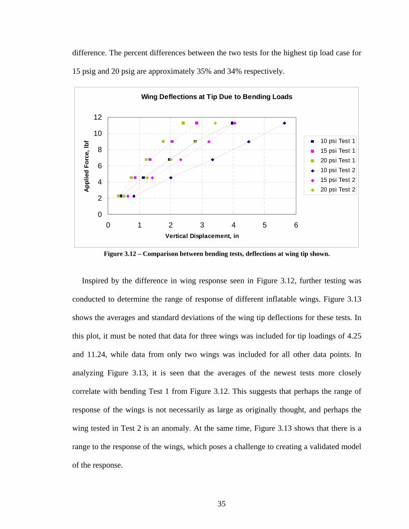
difference. The percent differences between the two tests for the highest tip load case for
15 psig and 20 psig are approximately 35% and 34% respectively.
Wing Deflections at Tip Due to Bending Loads
0
2
4
6
8
10
12
0 1 2 3 4 5 6Vertical Displacement, in
Appl
ied
Forc
e, lb
f 10 psi Test 115 psi Test 120 psi Test 110 psi Test 215 psi Test 220 psi Test 2
Figure 3.12 – Comparison between bending tests, deflections at wing tip shown.
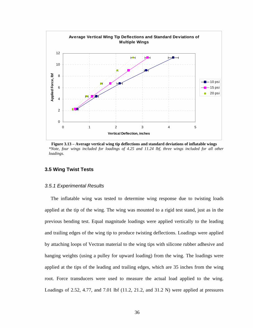
Inspired by the difference in wing response seen in Figure 3.12, further testing was
conducted to determine the range of response of different inflatable wings. Figure 3.13
shows the averages and standard deviations of the wing tip deflections for these tests. In
this plot, it must be noted that data for three wings was included for tip loadings of 4.25
and 11.24, while data from only two wings was included for all other data points. In
analyzing Figure 3.13, it is seen that the averages of the newest tests more closely
correlate with bending Test 1 from Figure 3.12. This suggests that perhaps the range of
response of the wings is not necessarily as large as originally thought, and perhaps the
wing tested in Test 2 is an anomaly. At the same time, Figure 3.13 shows that there is a
range to the response of the wings, which poses a challenge to creating a validated model
of the response.
35
Average Vertical Wing Tip Deflections and Standard Deviations of Multiple Wings
0
2
4
6
8
10
12
0 1 2 3 4 5
Vertical Deflection, inches
App
lied
Forc
e, lb
f
10 psi
15 psi
20 psi
Figure 3.13 – Average vertical wing tip deflections and standard deviations of inflatable wings
*Note, four wings included for loadings of 4.25 and 11.24 lbf, three wings included for all other loadings.
3.5 Wing Twist Tests
3.5.1 Experimental Results
The inflatable wing was tested to determine wing response due to twisting loads
applied at the tip of the wing. The wing was mounted to a rigid test stand, just as in the
previous bending test. Equal magnitude loadings were applied vertically to the leading
and trailing edges of the wing tip to produce twisting deflections. Loadings were applied
by attaching loops of Vectran material to the wing tips with silicone rubber adhesive and
hanging weights (using a pulley for upward loading) from the wing. The loadings were
applied at the tips of the leading and trailing edges, which are 35 inches from the wing
root. Force transducers were used to measure the actual load applied to the wing.
Loadings of 2.52, 4.77, and 7.01 lbf (11.2, 21.2, and 31.2 N) were applied at pressures
36

ranging from 10 to 25 psig, in increments of 5 psig. With the 11.75-inch chord-wise
separation between the applied vertical loads, the applied moments are 29.6, 56.0, and
82.4 lb-in, respectively. Both clockwise and counterclockwise twisting loads were
examined. Figure 3.14 shows the wing pressurized to 25 psig with applied loadings of
7.01 lbf (31.2 N) upward at the wing tip leading edge and downward at the wing tip
trailing edge.
Figure 3.14 – Wing under 7.01 lb couple forces for twist loading and 25 psig internal pressure. Vertical deflection was measured at several points along the span of the wing at the
leading and trailing edges. Results are shown in Figure 3.15 for a counterclockwise
twisting load and internal pressure of 15 psig. Clockwise loading results are not shown
but Figure 3.15 is representative of the negative of the deflections for clockwise loading.
In Figure 3.15, the leading edge vertical deflection under twisting load is seen to be less
than that of the trailing edge. Note that data points corresponding to 0 lbf loading are
deflections after the largest loading was removed, again showing hysteresis in the wing
response. The leading edge shows only small final displacements along the span after
37

unloading. However, the trailing edge shows final unloaded displacements similar to the
lowest loading and increasingly larger along the span to the wing tip. Incremental
unloading was not measured. Figure 3.16 presents the dependence of the wing deflections
on internal pressure. The deflections of the leading and trailing edges are larger for
smaller internal pressures. The difference among the leading edge deflections over the
range of all the pressures is much smaller than that of the trailing edge deflections. In
addition to the hysteresis of the system that is evident from Figure 3.15, it can be seen
from both results that the trailing edge of the wing is less stiff than the leading edge for
all load cases.
15 psi Internal Pressure
-3.5
-3.0
-2.5
-2.0
-1.5
-1.0
-0.5
0.0
0.5
1.0
1.5
0 5 10 15 20 25 30 35 40
Semi-span Station (in)
Verti
cal D
efle
ctio
n (in
) Trailing Edge 2.5 lbfTrailing Edge 4.8 lbfTrailing Edge 7.0 lbfTrailing Edge 0 lbf *Leading Edge 2.5 lbfLeading Edge 4.8 lbfLeading Edge 7.0 lbfLeading Edge 0 lbf *
Figure 3.15 – Wing deflections, 15 psig internal pressure.
*Corresponds to deflections after all loading removed, not before loading applied
38

82.4 lb-in Torque Loading Applied at Wing Tip
-4.0
-3.0
-2.0
-1.0
0.0
1.0
2.0
0 5 10 15 20 25 30 35 40
Semi-span Station, in
Vert
ical
Def
lect
ion,
in
Trailing Edge 10 psigTrailing Edge 15 psigTrailing Edge 20 psigTrailing Edge 25 psigLeading Edge 10 psigLeading Edge 15 psigLeading Edge 20 psigLeading Edge 25 psig
Figure 3.16 – Wing deflections, 82.4 lb-in applied torque.
Angle of Twist, 82.4 lb-in Applied Torque at Wing Tip
0.0
5.0
10.0
15.0
20.0
25.0
30.0
0 5 10 15 20 25 30 35 40
Semi-span Station, in
Ang
le o
f Tw
ist,
degr
ees
10 psig15 psig20 psig25 psig
Figure 3.17 – Angle of twist of wing for 82.4 lb-in applied torque.
Figure 3.17 shows the angle of twist vs. semi-span station due to an applied torque of
82.4 lb-in, for all tested pressure cases. This figure shows the angle of twist due to a
39

counterclockwise torque load on the wing (leading edge deflected upward, trailing edge
deflected downward). Clockwise torque results are similar. In Figure 3.17, the angle of
twist was calculated using the local chord length and measured deflections of the leading
and trailing edges.
3.5.2 Wing Torsional Stiffness Calculations
The following results could be used for future design considerations, or by researchers
interested in developing equivalent beam models of the inflatable wings.
Similar to the bending results above, treating the wing as a linearly elastic cantilever
beam with a torque load at the tip, the flexural rigidity of the wing can be calculated from
Equation (3-4).[39]
φ
TLGI p = (3-4)
Where: GIp = Torsional rigidity T = Applied torque load L = Beam length φ = Angle of twist The resulting torsional rigidity calculations are plotted in Figure 3.18, for the three
torque loadings considered and an internal pressure of 10 psig. The results vary for each
loading and pressure similarly for each point along the semi-span of the wing; however,
due to the scales of Figure 3.18 and Figure 3.19, this is not evident. However, if each
span location is plotted separately, results resemble those near the wing root in Figure
3.18 and Figure 3.19.
40

10 psig Internal Wing Pressure CCW Twist
0
200000
400000
600000
800000
1000000
1200000
0 5 10 15 20 25 30 35 40
Semi-span Station, in
Tors
iona
l Rig
idity
, lb*
in2
29.6 lb-in56.0 lb-in82.4 lb-in
Figure 3.18 – Torsional rigidity of wing for 10 psig internal pressure.
82.4 lb-in Applied Torque CCW Twist
0
200000
400000
600000
800000
1000000
1200000
1400000
1600000
1800000
2000000
0 5 10 15 20 25 30 35 40
Semi-span Station, in
Tors
iona
l Rig
idity
, lb*
in2
10 psig15 psig20 psig25 psig
Figure 3.19 – Torsional rigidity of wing for 82.3 lb-in torque applied at wing tip.
41

CHAPTER 4: FINITE ELEMENT MODELING OF STATIC LOAD CASES
This chapter details the efforts of simulating static load cases on the inflatable wing
and presents comparisons of these simulations to the experimental tests discussed in
Chapter 3.
The process of developing the FE model of the wing began with a previous
“pathfinder” model by Nathan Coulombe, defined and evaluated as part of an
undergraduate independent study course. His model was constructed using shell elements
with Young’s modulus material properties discussed in Section 3.1 for the Urethane-
coated Vectran. The pathfinder model proved too stiff when compared to experimental
results. The test data discussed in Section 3.2 was sent to UK by ILC Dover, and simpler
models of inflatable test cylinders were considered to determine the validity of the
modeling approach.
After these models were validated through comparisons with experimental data, focus
shifted back to the wing model, and correlation of the FE model to experimental static
loading. Initially, a linear orthotropic material model with different Young’s Moduli in
the warp and fill directions was considered, with final “effective” moduli being
determined by modifying the moduli values and comparing FE simulations to
experimental results. This process led to the conclusion that the FE model was in general
too stiff. Subsequently, the mesh density of the model was varied to first verify that the
model was meshed sufficiently to reach a converged solution, and then to reduce solution
time. These mesh density studies were conducted in parallel with models incorporating a
nonlinear isotropic material model that more closely resembles the true stress-strain
curves of the Vectran material.
42

It should be noted that the order of presentation throughout this chapter is not
necessarily chronological. Also note that the term “model” in this section refers to the FE
model, and when referring to material data models, the term “material model” will be
used. All pressures are gage pressure.
4.1 FE Analysis of Shear Test Cylinders
For validation purposes, finite element models of the urethane-coated test cylinders
were created using ANSYS (version 8.0). The goal here was to use these models to
simulate the shear modulus tests discussed in Section 3.2. A cylindrical model was
created using single-layer orthotropic shell elements (SHELL181) for the surface of the
cylinder. The length of the model was 15 inches, corresponding to the distance between
the two end clamps on the test stand. Nodes at the “fixed” end of the cylinder were
constrained in all directions. Multipoint constraint (MPC184) elements were used to
apply the load torque on the opposite end of the cylinder. Constraint elements were
attached to the free end of the cylinder and to a master node (for torque application)
located two inches beyond the end of the cylinder on the centerline. Also, models with
both coarse and fine meshes were created. With all constraints applied, the coarse model
contained 385 nodes and 2166 DOF, while the fine model contained 1861 nodes and
10,806 DOF. These finite element meshes are shown in Figure 4.1.
Two models were created, corresponding to the two test cylinders. One model had
warp material properties in the longitudinal direction, and fill properties in the hoop
direction, while the other model had the directions of these two material property
orientations interchanged. The same basic model was used for both test cylinders, with
43

only the longitudinal- and hoop-direction material properties different between them. A
linear orthotropic material model was used, with the properties shown in Table 4.1.
Figure 4.1 – FE model of inflatable test cylinders with coarse (left) and fine (right) meshes
Table 4.1 – Vectran material properties used in the cylinder model Material Property
Value
Fill Modulus 1.22 MsiWarp Modulus 1.36 MsiShear Modulus Variable*
Thickness 0.013 in*For each case, the appropriate shear modulus was used from the test data
depending on the internal pressure applied to the model.
For each case of different pressure loading, the solution process represents the
experimental sequence. First, internal pressure loading was applied to the cylinder, and
the nonlinear static solution was obtained. Once this solution was obtained, the
appropriate torque was applied to the master node at the free end of the cylinder. The
model was solved again, including the stress-stiffening effects of the pressure solution.
For both solution steps, a nonlinear analysis was performed to account for large
deflections and stress stiffening.
44

Comparisons between the results of the FE analyses and the experimental data for an
internal pressure of 1 psi can be seen in Figure 4.2 and Figure 4.3. In these figures,
circumferential displacement, the distance any point at the cylinder tip travels in the
direction of the circumference of the cylinder, is plotted to allow for ease of comparison
of experimental to FE results. These results are representative of results at higher
pressures.
Longitudinal Warp Results - 1 psig Internal Pressure
0.00
20.00
40.00
60.00
80.00
100.00
120.00
0.00 0.05 0.10 0.15 0.20 0.25 0.30 0.35
Circumferential displacement, in
Appl
ied
Torq
ue, i
n*lb
Exp. DataFEA Coarse MeshFEA Fine Mesh
Figure 4.2 – Comparison of results from cylinder with longitudinal warp, 1 psi internal pressure
45

Hoop Warp Results - 1 psig Internal Pressure
0.00
20.00
40.00
60.00
80.00
100.00
120.00
0.00 0.05 0.10 0.15 0.20 0.25 0.30 0.35
Circumferential Displacement, in
Appl
ied
Torq
ue, i
n*lb
Exp. DataFEA Coarse MeshFEA Fine Mesh
Figure 4.3 – Comparison of results from cylinder with hoop warp, 1 psi internal pressure.
There proved to be little difference between the fine and course FE model results. It
was therefore determined that a course mesh would be sufficient and would reduce
solution times. In both orientations, the FE model results have slopes that generally
correlate to those of the plotted experimental data.
For the longitudinal warp orientation and loads greater than 30 in-lb, the FE analysis
angular deflection results are greater than the experimental data by a near constant
difference. Both the experimental and FE results for the longitudinal warp orientation are
linear or nearly so. For the longitudinal fill (hoop warp) orientation in Figure 4.3, the
experimental data shows a nonlinear softening trend, so the FE model and experimental
results do not correlate as well for all load cases at this lowest pressure. A linear
approximation for the moduli appears to be less accurate for fill shear modulus, as can be
seen from the experimental data.
Also, the experimental data shows an initial angular deflection of the cylinder even
when no torque has been applied. Initial twist was in the same direction as the loading.
For the longitudinal fill cylinder, initial twist ranged from 2.2 – 5.0 degrees, and
46

decreased as pressure increased. For the longitudinal warp cylinder, initial twist ranged
from 5.6 – 6.4 degrees, and increased as pressure increased. Initial twist in the cylinders
may be due to initial twist in the cylinder during test set-up, or may possibly come from
inherent properties of the weave in the Vectran. This initial twist was not present in the
FE results. For comparison between experimental deflection and FE deflection, the initial
twist was subtracted from the loaded twist.
Furthermore, it is important to note that when the model is loaded with pressure only,
the computed radial deflection of the cylinder in all cases is much less than the radial
deflection recorded experimentally. Knowing that the radial deflection of the cylinder FE
models due to pressure loading did not match the radial deflection seen in the laboratory
testing, various factors were applied to reduce the Young’s moduli in the warp and fill
directions in the FE model, until the radial deflection of the model matched the radial
deflection seen in laboratory testing.
The fact that the urethane coating of the test cylinders would make the material more
stiff than the silicone-coated Vectran used in the wings also motivated determination of a
reduction factor to apply to the cylinder material properties to be used in the inflatable
wing model. For correlation of the radial deflections, the urethane-coated Young’s
moduli were reduced to 25% of the values used for the initial model.
Although a few questions remain for the correlation of the cylinder model to the
available data, the correlation seen in Figure 4.2 and Figure 4.3 is sufficient for use in the
initial FE model of the internally pressurized Vectran wing.
47

4.2 FE Model of Inflatable Wings
4.2.1 FE Model Geometry
ANSYS finite element software was used to create the finite element model of the
inflatable wing. The profile of the wing root was initially modeled in ProEngineer™ from
cross section drawings provided by ILC Dover, shown in Figure 4.4. This profile was
imported into ANSYS, and the resulting keypoint locations were recorded. These
keypoint locations were then included in an ANSYS batch file (See Appendix A) to
remove the step of importing a geometry file each time the model was created.
For modeling purposes, an assumption was made that each inflated section of the wing
had a cross section shape composed of circular arcs for the external restraint and straight
lines for the internal spars. The cross-section of the wing tapers linearly along the span
from the root to the tip, so the complete geometry was created in ANSYS by scaling
down the root profile to create the tip profile, then “connecting” the two profiles with
areas that create the external restraint and internal spar areas. Rather than trying to
reproduce the detail for the rounded seamed tip of the wing, a flat end was meshed to
allow pressure forces to stiffen the restraint elements along the span-wise direction. The
actual wing has a nominal semi-span of 36 in. with leading and trailing edge lengths of
35 in. For the FE model, due to the simplification of modeling a flat wing tip, the semi-
span length for the wing, including both leading and trailing edges, is 36 in. The seams
present in the wing were not included in the FE model. Rather, the internal spars were
modeled with a rigid connection to the external restraint. The internal bladder was not
included in the FE model. Because the internal volume of the bladder is larger than the
48

internal volume of the restraint, an assumption was made that the two layers would align
and act as one, and the Vectran material properties would dominate wing response.
The geometry was then meshed as shown in Figure 4.5. ANSYS shell (SHELL181)
elements were used. These are four-node elements with six degrees of freedom per node
and are suitable for thin to moderately-thick shell structures [40]. An element thickness
value of 0.013 in. was used, which is the nominal thickness of the Vectran fabric. As seen
in Figure 4.5, the FE mesh was created such that spanwise mesh density increases toward
the wing tip, with the element length at the tip being ½ the element length at the root.
Spanwise elements were created using the mapped mesh option in ANSYS, while the flat
wing tip area was meshed with a free mesh. As in the physical wing, the wing tip area
was connected only to the external restraint and not to the internal spars. This initial
model contained 17,681 elements and 16,887 nodes. All nodes at the wing root were
constrained in all DOF, simulating the cantilever mount configuration. After these
constraints were applied, the initial model contained 100,428 DOF.
Figure 4.4 – Wing dimensions in inches
49

Figure 4.5 – Meshed inflatable wing model
4.2.2 Mesh Convergence
From the initial correlation comparisons, it was seen that the FE model proved stiffer
than the wing. In order to confirm that the model mesh contained enough DOFs to reach
a converged solution and that the mesh density was not artificially stiffening the model, a
finer mesh was constructed. This fine mesh contained 139,866 DOF, a 39% increase from
the 100,428 DOF in the original model. This model was solved for a loading case of 10
psi internal pressure and an upward bending tip load of 11.24 lbf (50 N). For both linear
and nonlinear material models, the finer mesh showed no change in the deflection results,
thus the original mesh was determined to be sufficient for obtaining static solutions.
Once it was seen that increasing the mesh density had no effect on the solution, a more
coarse mesh was considered in an effort to reduce solution computation time. This coarse
model contained 69,750 DOF after all constraints were applied. When this mesh was
considered along with the linear material model, the solver failed to converge to a
solution, even after increasing the number of solution iteration substeps. However, the
nonlinear material model did converge with this coarse mesh to the same result as seen
50
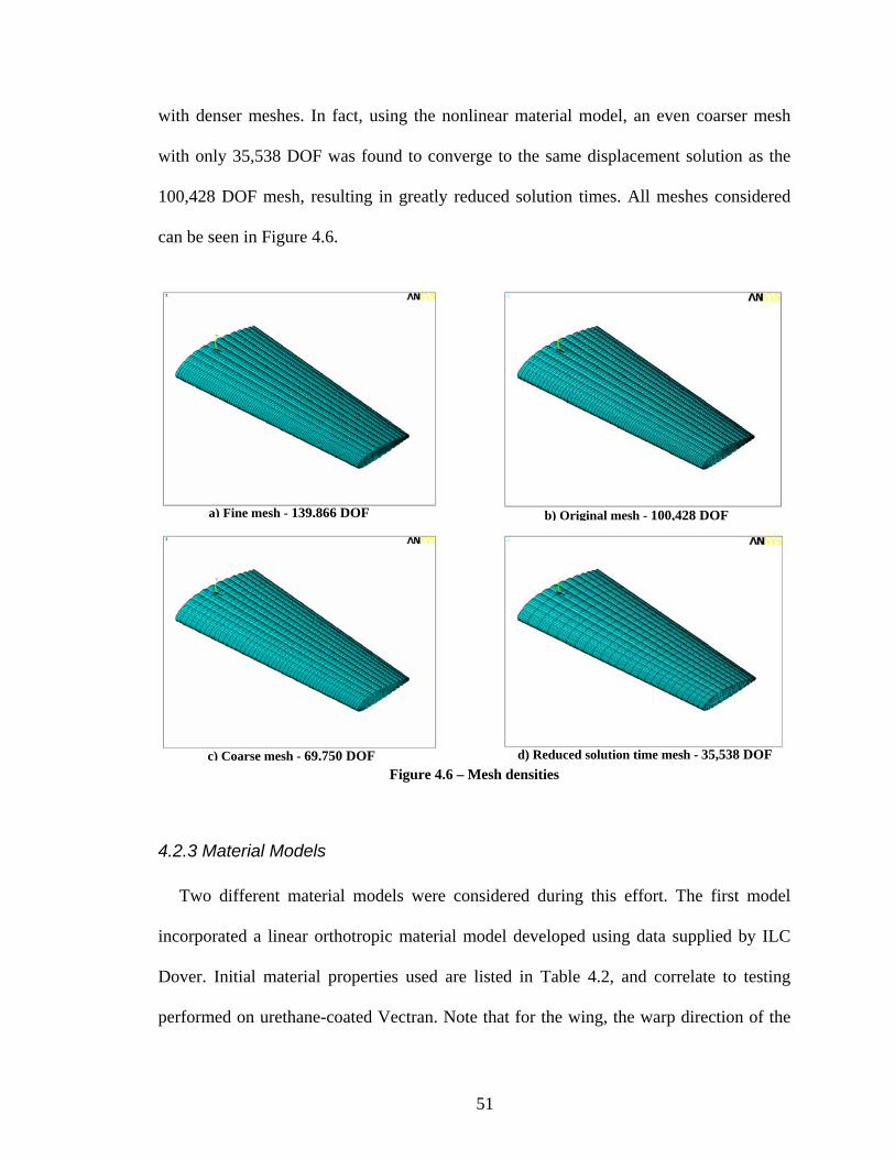
with denser meshes. In fact, using the nonlinear material model, an even coarser mesh
with only 35,538 DOF was found to converge to the same displacement solution as the
100,428 DOF mesh, resulting in greatly reduced solution times. All meshes considered
can be seen in Figure 4.6.
a) Fine mesh - 139,866 DOF b) Original mesh - 100,428 DOF
d) Reduced solution time mesh - 35,538 DOF c) Coarse mesh - 69,750 DOFFigure 4.6 – Mesh densities
4.2.3 Material Models
Two different material models were considered during this effort. The first model
incorporated a linear orthotropic material model developed using data supplied by ILC
Dover. Initial material properties used are listed in Table 4.2, and correlate to testing
performed on urethane-coated Vectran. Note that for the wing, the warp direction of the
51

fabric restraint is oriented parallel to the wing span and the fill direction is oriented
parallel to the wing chord. The fabric of the internal spars is also oriented with the warp
direction parallel to the wing span. At the time of initial model creation, the urethane
coating material properties were the only data available, though it was later determined
that the wings were actually constructed of silicone-coated Vectran, and that the different
coatings can have a large effect on the material properties. Using the urethane material
properties, the model initially proved too stiff, and effective moduli were determined
through FE bending load simulations. This process, including determination of effective
moduli, is discussed in detail in Section 4.3.1.1.
Table 4.2 – Initial material properties used in FE model Material Property
Value
Fill Modulus 1.22e3 ksiWarp Modulus 1.36e3 ksiShear Modulus 200 ksi
Upon revisiting the tensile test data of the Vectran material, it was seen that the full
stress-strain curves for the warp and fill directions of the fabric are nonlinear, so a second
material model was developed for use in the FE model. Figure 4.7 shows the full stress
strain curves obtained from tensile testing, with five strips of Vectran being tested in each
of the warp and fill directions. Because the stress-strain curves in Figure 4.7 are similar
(neglecting outlier fill sample 1), the nonlinear isotropic material model shown in Figure
4.8 was developed for use in the FE model. The multilinear curve shown was used to
allow for ease of input into the FE model.
52

Figure 4.7 – Tensile test stress-strain diagrams for both material directions.
0 0.02 0.04 0.06 0.08 0.1 0.12 0.140
0.5
1
1.5
2
2.5
3
3.5x 10
4 Nonlinear Material Model for FE Analysis
Strain
Stre
ss, p
si
Figure 4.8 – Material model used in the FE model.
4.2.4 Application of Loads
The model solution process consisted of two steps. First, before applying external
loads to the wing model, internal pressure was applied. All nodes at the wing root were
constrained in all DOF, and pressure loading was applied outward to the elements
53

comprising the external surfaces to simulate the pressurization of the wings. This
includes the wing tip area. Initially, four different cases were to be considered: 10, 15, 20
and 25 psi. The Newton-Raphson nonlinear solver was used to compute static response to
account for large deflections and stress stiffening. For pressures higher than 15 psi, this
pressure solution failed to converge, even after increasing the number of iteration
substeps used.
Once the internal pressure loading solution was obtained, external loadings were
applied and subsequent solutions were computed, for both external bending loads and
external twisting loads.
4.3 FE Simulations of Static Loads
4.3.1 Wing Bending
After the initial pressurization analysis converged, an upward vertical force was
applied at the node corresponding to the location of the applied force in the experimental
bending test, and vertical deflection results were obtained at nodes corresponding to
measurement locations from the experimental bending test. Application of the internal
pressure loading caused initial deflections to the wing, and these positions were
subtracted from the final loading deflections to determine the calculated displacements
for comparison to experimental results.
4.3.1.1 Linear Orthotropic Material Model
In Figure 4.9, applied load vs. vertical deflection is plotted for an internal pressure of
10 psi. Data from two experimental tests was available for initial comparisons. Due to the
lengthy solution time of each FE analysis, in the following sequence, material properties
were adjusted to obtain correlation of the model for the lowest wing tip loading case
54

before the model solution was computed for higher tip loadings. The initial finite element
model used a linear orthotropic material model, with urethane-coated warp and fill
moduli and shear modulus as determined from experimental testing. Loads were applied,
and this model did not converge to a solution. The large difference between E = 1.36e3
ksi and G = 15 ksi was thought to be a problem, so a temporary shear modulus of G =
200 ksi was used in the FE model to achieve initial convergence. This adjusted shear
model proved to be more stiff than the wing was seen to be through experimental testing,
so a reduction factor was applied to the material properties to obtain “effective” moduli
for the model. Because the Young’s moduli would affect the stiffness of the wing in
bending more than the shear modulus, the Young’s moduli were reduced while shear
modulus was initially kept constant at 200 ksi.
Results of various modulus factors are also shown in Figure 4.9 for 10 psi internal
wing pressure and 2.25 lbf loading, highlighted in the plot. It was found that a value of
25% of the original Young’s modulus still proved too stiff, while 5% was too soft.
Correlation to experimental results was achieved for this load case with a modulus
reduced to 8% of the urethane test value. After results matched well for this case, the
model solution was computed for higher tip loadings using the same 8% reduced
modulus. Finally, with converging solutions at this lower Young’s moduli, the shear
modulus was reduced from 200 ksi to 20 ksi, much closer to the value found from
material testing. However, as can be seen in Figure 4.9, this change had only a minimal
effect on the final calculated deflections. In examining Figure 4.9 it can be seen that for
an internal wing pressure of 10 psi, FE and experimental results matched well only for tip
loadings below 4.5 lbf and diverged significantly after that.
55

Figure 4.9 – Comparison of experimental and FE wing deflection results
In Figure 4.10, results for bending deflections of a wing with internal pressure 15 psi
are shown. It is seen that for this case, FE results actually match well with experimental
results. However, it should be noted that FE results for 10 psi and 15 psi are nearly
equivalent. Thus, it is seen that the bending stiffness of the wing model does not increase
with pressure as the actual wing does. A shear modulus of 50 ksi was used for the 15 psi
case to enable convergence of the solution, but as noted previously, varying the shear
modulus has only a minimal effect on the deflection results. Also, higher pressures of 20
and 25 psi did not converge to a solution, even after using larger shear modulus values
and applying a higher number of solution iterations. However, it should be noted that
wing warping strategies being investigated are most effective at lower wing inflation
pressures, so modeling capability in this achievable pressure range is preferred for
research on this topic.
56

Deflection at Point 1 - 15 psig Internal Pressure
0
2
4
6
8
10
12
-0.500 0.000 0.500 1.000 1.500 2.000 2.500 3.000
Vertical Deflection, in
Appl
ied
Load
, lbf
ExperimentalFEA E=8% G=50 ksi
Figure 4.10 – Comparison of experimental and FE wing deflection results.
Although results were mixed for correlation of the FE model of the inflated wing to
experimental results, important characteristics were accurately modeled. For example,
Figure 4.11 is the resulting deflected shape with 15 psi inflation pressure and 11.2 lbf tip
force. As expected, the maximum deflection occurs at the tip with a characteristic beam-
bending profile along the span. As with the experiment, no twisting is seen in the
deflected result.
Note also that at the time of the initial modeling effort, only urethane-coated Vectran
moduli were available, so a reduced modulus was determined for the wing. After this was
completed, Young’s moduli for the silicone-coated material became available and were
seen to be 20% of that of the urethane-coated material. The reduced moduli determined
through the validation effort ranged from 5% – 25% of the urethane-coated moduli, with
8% providing the best correlation for 10 psi internal pressure and 2.25 tip loading.
57
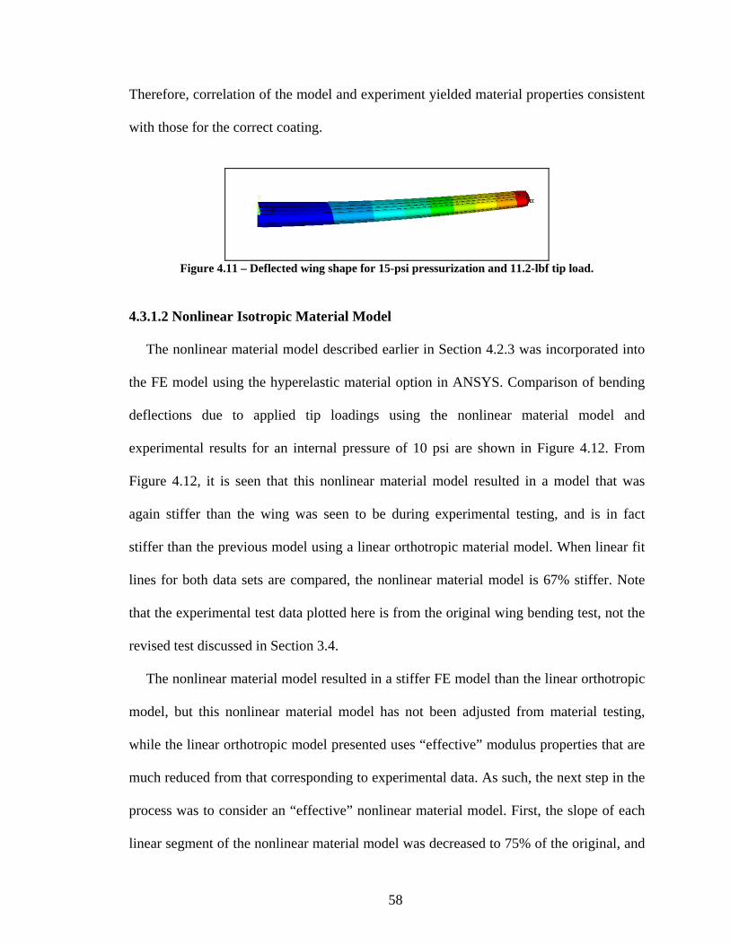
Therefore, correlation of the model and experiment yielded material properties consistent
with those for the correct coating.
Figure 4.11 – Deflected wing shape for 15-psi pressurization and 11.2-lbf tip load.
4.3.1.2 Nonlinear Isotropic Material Model
The nonlinear material model described earlier in Section 4.2.3 was incorporated into
the FE model using the hyperelastic material option in ANSYS. Comparison of bending
deflections due to applied tip loadings using the nonlinear material model and
experimental results for an internal pressure of 10 psi are shown in Figure 4.12. From
Figure 4.12, it is seen that this nonlinear material model resulted in a model that was
again stiffer than the wing was seen to be during experimental testing, and is in fact
stiffer than the previous model using a linear orthotropic material model. When linear fit
lines for both data sets are compared, the nonlinear material model is 67% stiffer. Note
that the experimental test data plotted here is from the original wing bending test, not the
revised test discussed in Section 3.4.
The nonlinear material model resulted in a stiffer FE model than the linear orthotropic
model, but this nonlinear material model has not been adjusted from material testing,
while the linear orthotropic model presented uses “effective” modulus properties that are
much reduced from that corresponding to experimental data. As such, the next step in the
process was to consider an “effective” nonlinear material model. First, the slope of each
linear segment of the nonlinear material model was decreased to 75% of the original, and
58

10 psi internal pressure and bending loads were simulated. To reduce solution processing
time, the coarse FE mesh containing 69,750 DOF was used for these analyses. The
reduced solution time 35,538 DOF mesh failed to converge to a solution when this
adjusted material model was used. The results for this material model are also plotted in
Figure 4.12. From this plot it can be seen that this material model more closely models
the response of the wing compared with the original nonlinear material model, but still
proves 18% stiffer than the linear orthotropic model over the range of pressures
considered. However, this difference in the adjusted and original nonlinear models is less
than the difference between the original and “effective” linear material models, so the
nonlinear model more closely correlates to what was seen during material testing.
Figure 4.13 shows a comparison of bending deflections due to applied tip loadings
using the nonlinear material model and experimental results for an internal pressure of 15
psi. Of important note for this pressure case is that the modified nonlinear material model
resulted in a FE model that actually deflected farther than the wing deflected
experimentally, and in fact deflected farther than the FE model under 10 psi internal
pressure. It should be noted that the 10 psi cases were computed using a coarser mesh
than the 15 psi case because the 15 psi case failed to converge to a solution using a mesh
coarser than the original mesh. Initially, this was thought to be the cause of the modified
material model causing these larger deflections. However, when the 10 psi case was re-
computed with the original mesh, the results did not change, so the mesh density is not
the reason for this softening effect in the 15 psi case. With this result, no further
adjustment of the nonlinear material model was considered.
59

Deflection at Wing Tip - 10 psig Internal Pressure
0
2
4
6
8
10
12
-1.000 0.000 1.000 2.000 3.000 4.000 5.000
Vertical Deflection, in
App
lied
Load
, lbf
Exp Test 1
FEA Linear OrthotropicMaterialFEA Nonlinear IsotropicMaterialFEA Nonlinear Isotropic, 75%of Original
Figure 4.12 – Comparison of experimental and FE wing bending results for 10 psi, deflection at wing tip shown.
Deflection at Point 1 - 15 psig Internal Pressure
0
2
4
6
8
10
12
0.000 0.500 1.000 1.500 2.000 2.500 3.000 3.500
Vertical Deflection, in
Appl
ied
Load
, lbf
Experimental
FEA Linear Orthotropic Material
FEA Nonlinear Isotropic Material
FEA Nonlinear Isotropic Material75%
Figure 4.13 – Comparison of experimental and FE wing bending results for 15 psi, deflection at wing tip shown
60

4.3.2 Wing Twist
Starting with the correlated wing models from the previous section, computed FE
model deflections were compared to experimental results for torsion loading. Similarly to
the case of modeling wing bending, the process of modeling an inflatable wing under a
wing tip torsion load began with applying internal pressure to the FE model. After the
internal pressure loading converged to a solution, vertical loads were applied to nodes at
the leading and trailing edges of the FE model in opposite vertical directions to create the
torsion load applied in laboratory testing. Vertical forces of 2.52, 4.77, and 7.01 lbf were
analyzed in separate cases. Vertical deflection results were obtained for nodes along the
leading and trailing edges of the FE model, at semi-span stations corresponding to
measurement points from the experimental torsion test.
4.3.2.1 Linear Orthotropic Material Model
Figure 4.14 shows a comparison between experimental measurements and FE
predictions of the angle of twist at the wing tip due to an applied torque Both 10 psi and
15 psi results are included, for both experimental data and FE results. The angle of twist
was computed using the calculated deflections of the leading and trailing edge points.
The results show that the inflatable wing FE model is also too stiff in torsion. While for
the wing bending case, at 15 psi internal pressure, FE and experimental models correlated
well, this is not the case for torsion loading at the same internal pressure. FE models of
both 10 and 15 psi cases were found to deflect much less than expected from
experimental testing. For 10 psi internal pressure, computed angle of twist at the wing tip
was on average only 16% of experimentally determined angle of twist. For 15 psi,
computed results on average were 29% of experimental.
61

While the deflection magnitudes from the FE analysis are less than those seen in the
experimental testing of the wing, the deformed plot in Figure 4.15 shows that the FE
model deflected shape does generally match the deflected shape seen in laboratory
testing. Most notably, it can be seen in Figure 4.15 that the trailing edge deflects more
than the leading edge, which, can clearly be seen from Figure 3.14 to be the case for the
actual wing under load as well.
The same material model and material properties used in the FE model for the bending
test were used for the torsion loading case, with one exception: when a positive (trailing
edge upward, leading edge downward) torsion load was applied to the wing, at 10 psi,
using a shear modulus of 20 ksi, the model failed to converge to a solution. As such, the
shear modulus was increased to 50 ksi for this loading case. Just as for the wing bending
case, internal pressures higher than 15 psi failed to converge to a solution.
Angle of Twist at Wing Tip
0.0
10.0
20.0
30.0
40.0
50.0
60.0
70.0
80.0
90.0
0.000 5.000 10.000 15.000 20.000 25.000
Angle of Twist, degrees
Appl
ied
Torq
ue, l
b-in
Experimental 10 psi Experimental 15 psi FEA 10 psiFEA 15 psi
Figure 4.14 – Comparison of angle of twist at wing tip, negative twist applied.
62

Figure 4.15 – Deflected wing shape for 15-psi pressurization and 82.4-lb-in tip load.
*results scaled X 2 for clarity.
4.3.2.2 Nonlinear Isotropic Material Model
Torque loadings were also modeled using the two nonlinear isotropic models. Figure
4.16 shows the resulting angle of twist at the wing tip due to applied torques of 29.6 and
82.4 lb-in, at a wing inflation pressure of 10 psi. Similarly to the bending cases, the linear
orthotropic model most closely estimates the experimental results, and the adjusted
nonlinear isotropic model is more accurate than the original nonlinear isotropic model.
63

Angle of Twist at Wing Tip
0.0
10.0
20.0
30.0
40.0
50.0
60.0
70.0
80.0
90.0
0.000 5.000 10.000 15.000 20.000 25.000
Angle of Twist, degrees
App
lied
Torq
ue, l
b-in Experimental
FEA Linear Orthotropic Material
FEA Nonlinear Isotropic Material
FEA Nonlinear Isotropic Material,75% of Original
Figure 4.16 – Comparison of experimental and FE angle of twist at wing tip due to applied torques
4.4 Simulation of Wing Warping
One objective of this effort is to develop a model which can be used to evaluate wing
warping actuation designs. Figure 2.8 shows an example of a wing warping technique
applied to a low pressure inflatable wing. One or more servos are mounted to the wing in
a manner to actuate motion of the trailing edge. Warping designs and associated wind
tunnel studies are included in the research conducted by Simpson [29]. Rather than
applying a moment to an aileron for roll control, the moment is applied directly to the
wing, changing the wing profile as seen in Figure 2.8. Inspired by this method of wing
warping, the FE model was used to simulate wing response to moment loadings applied
by multiple servos along the span of the wing.
For this simulation, the reduced solution time mesh containing 35,538 DOF was used
in order to keep solution computation time to a minimum. The nonlinear isotropic
64

material model was used. As in previous simulations, two load steps were considered, the
first step was two apply internal pressure, and the second step was to apply the moment
loadings. Figure 4.17 presents the locations of the applied moments. Note that area
normals for the elements are reversed here only for ease of visualization, and in the
analysis, the element area normals were oriented similarly to the other elements on the
wing. Each “patch” area contains 30 elements, and 48 nodes. Moments of 8 lb-in were
applied to the areas by applying moments of 0.167 lb-in to each node.
The load patterns considered are listed in Table 4.3. Moments are applied in the global
X-direction, with the global X-axis being perpendicular to the wing cross section with
positive orientation being the direction from the wing root toward the wing tip. As such, a
negative moment acts as a servo “pulling” the trailing edge downward similar to the
deformation shown in Figure 2.8, while a positive moment acts as a servo “pushing” the
trailing edge upward.
65

Patch 2
Patch 1 + X dir.
Patch 3
Bottom of Wing Shown
Figure 4.17 – Locations of applied moments on underside of wing
Table 4.3 – Loadings applied for each wing warping analysis Analysis Patch 1 Patch 2 Patch 3
1 - 8 lb-in 0 0 2 - 8 lb-in - 8 lb-in 0 3 - 8 lb-in - 8 lb-in - 8 lb-in 4 + 8 lb-in + 8 lb-in + 8 lb-in 5 - 8 lb-in + 8 lb-in - 8 lb-in
The analyses are intended as a qualitative demonstration of how the wing model can
be used to predict response to warping forces. Further modification of the model is
needed to accurately predict wing deflections, as the model as is proves too stiff in
response to static loads. Figure 4.18 shows the resulting deflected shape of the wing from
a negative moment applied at Patch 1 only. As expected, the resulting shape shows the
wing tip trailing edge deflecting downward, much like the example in Figure 2.8. The
66

results shown here have been scaled up by 5X to effectively show the deflection at the
trailing edge, due to the over-stiffness of the model and the relative scale of the deflection
with respect to the overall dimensions of the wing. Figure 4.19 shows the resulting
deflection of the wing with negative moments applied at Patch 1 and Patch 2, while
Figure 4.20 shows the same for negative moments applied at all three Patches. The
resulting deflection at the wing tip trailing edge is plotted vs. the number of servos
considered in Figure 4.21.
Resulting wing deflection from Analysis 4, with positive moments applied at all three
Patch locations, is shown in Figure 4.22.
Figure 4.23 shows the deflected wing trailing edge shape resulting from Analysis 5
with negative moments applied at Patches 1 and 3 and a positive moment applied at Patch
2. Note the curvature of the trailing edge that can be obtained by using three servos to
apply loadings to the wing simultaneously.
67

Figure 4.18 – Analysis 1 resulting deflections. Scale increased by 5X.
Figure 4.19 – Analysis 2 resulting deflections. Scale increased by 5X.
68

Figure 4.20 – Analysis 3 resulting deflections. Scale increased by 5X.
Trailing Edge Deflection of Wing Tip
00.020.040.060.080.1
0.120.140.160.18
0 1 2 3
Number of Servos
Def
lect
ion,
inch
es
4
Trailing Edge Deflection of Wing Tip
00.020.040.060.080.1
0.120.140.160.18
0 1 2 3
Number of Servos
Def
lect
ion,
inch
es
4
Figure 4.21 – Predicted wing deflections vs. number of servos
69
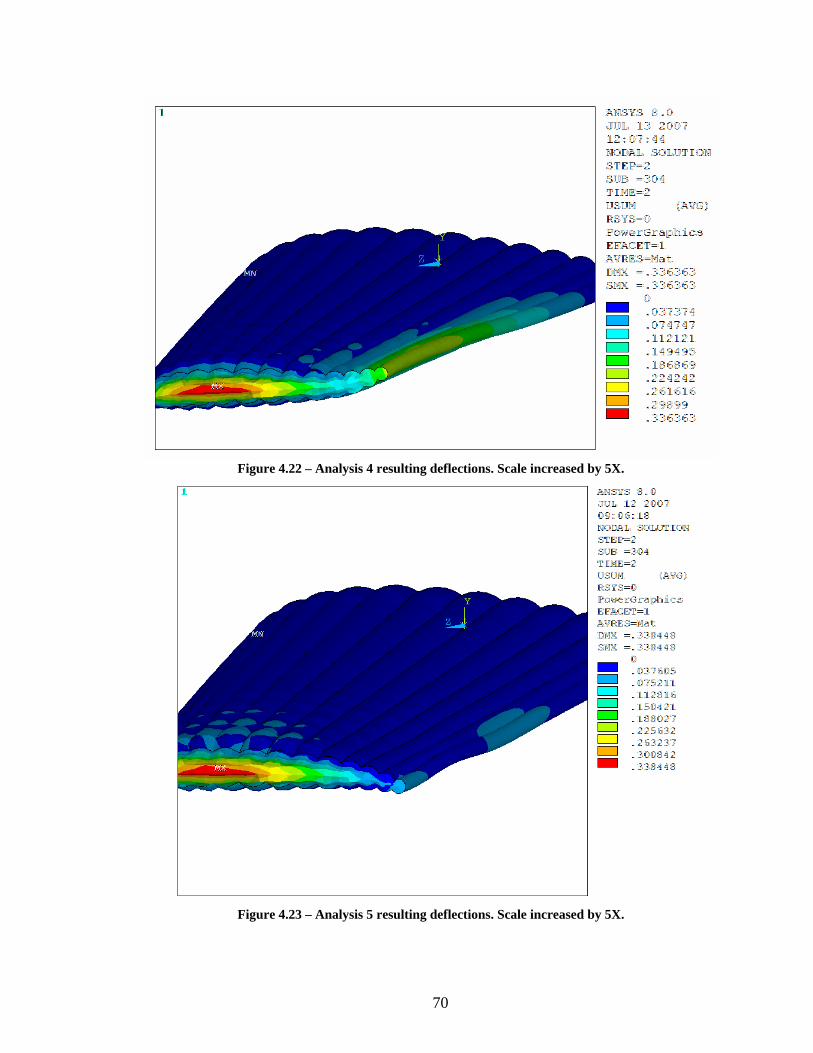
Figure 4.22 – Analysis 4 resulting deflections. Scale increased by 5X.
Figure 4.23 – Analysis 5 resulting deflections. Scale increased by 5X.
70

CHAPTER 5: EXPERIMENTAL AND FE MODAL ANALYSES
As inflatable wings do not have any rigid structural components, internal pressure is
required to maintain the airfoil profile. Thus, aeroelasticity of inflatable wings is of great
interest due to the wings flexibility. A major research area in the field of aeroelasticity is
flutter. Aeroplane Monthly defines flutter as “…the unstable oscillation caused by
interaction between aerodynamic forces, elastic reactions in the structure and the force of
inertia [41].” Flutter has the potential to increase without bounds given the right
conditions. In order to create a model that can be used to investigate these aeroelastic
phenomena the wing finite element model was adapted and vibrational testing was
conducted on the inflatable wings for model validation of structural dynamic response.
In this chapter, a verified finite element method modal analysis of an inflatable wing is
presented, beginning with experimental determination of vibrational characteristics of the
wing. Additionally, a discussion of the finite element model and solution processes is
presented, including both linear and non-linear applications of internal pressure loadings.
Finally, finite element results are compared to results of the experimental testing to
evaluate the model.
5.1 Experimental Modal Analysis
5.1.1 Test Setup
Even though the test article is a unique structural system, a standard experimental
modal analysis was conducted at first to determine if alternate testing approaches would
be required. A schematic of the test set-up is shown in Figure 5.1. A series of
cantilevered modal tests were performed to determine the vibrational characteristics of
71

the inflated wing under various internal pressures. The wing semi-span was mounted at
the root to a rigid test stand as shown in Figure 5.2. Small, lightweight uniaxial
accelerometers were secured to the Vectran restraint surface with silicone rubber
adhesive. These were located at the wing tip at two locations as shown in Figure 5.2: 1)
near the mid-chord of the wing and 2) near the trailing edge. These accelerometer
locations were chosen so that both bending and torsional vibrations could be recorded.
Impulse excitation was used for the modal testing by striking the wing with an impact
hammer. Inputs were applied at 10 locations on the wing as indicated in Figure 5.3,
including at the locations of the two accelerometers for driving-point measurements. The
test was repeated at wing pressures of 5, 10, 15, 20, and 25 psig.
Figure 5.1 – Block diagram of experimental test setup
72

Figure 5.2 – Photo of test setup showing placement of accelerometers
7
8
9
10
1
2
3
4
5
6
Figure 5.3 – Locations of excitation test points on the wing. Note that excitation points 9 and 10 are also measurement locations of accelerometers
73

Frequency Response Functions (FRFs), including magnitude and phase, and the
coherence of each input/output pair were calculated and recorded in universal file format
data files using a Zonic Medallion multichannel data acquisition system and signal
analyzer software. For the data acquisition and signal processing, a sampling frame size
of 2048 was used, along with a bandwidth frequency of 500 Hz, resulting in a frame
period of 1.6 seconds, with a frequency resolution of 0.625 Hz. Ten averages were used
at each measurement point. An exponential window was also used for processing of the
Fast Fourier Transforms (FFTs) used to compute the FRFs.
Typical FRF and coherence results for two simultaneous response measurements are
presented in Figure 5.4. This result is for a wing pressure of 15 psi, impulsive input at
Point 4 and measured acceleration response at both locations. The two sensors are located
so as to identify different modes of response, including bending and torsional modes.
Therefore, these FRFs are not expected to be identical. In the coherence plots, results
above 200 Hz are seen to degrade, while results below 200 Hz are good. For the
remainder of this chapter, results will be presented for the range 0 to 200 Hz, rather than
the full data range of 0 to 500 Hz.
74

0 100 200 300 400 50010
-2
100
102
Mag
nitu
de
Frequency Response Function
0 100 200 300 400 500-5
0
5
Phas
e
0 100 200 300 400 5000
0.5
1
Frequency, Hz
Coh
eren
ce
MidpointTrailing Edge
Figure 5.4 – FRFs of wing at both measurement points due to excitation at point 4, with wing internal pressure of 15 psi
5.1.2 Signal Processing and Typical Results
In order to determine the appropriate number of averages to use, tests were conducted
using thirty averages with results compared to those of tests using ten averages. Figure
5.5 and Figure 5.6 show the FRFs and coherances of the wing inflated to 20 psig with
impulsive input applied at test location 2. In Figure 5.5 and Figure 5.6, the blue data
represents the test using ten averages, while the red data represents the test using thirty
averages. For the frequency range of interest, (0 to ~200 Hz), there is essentially no
difference between the two results. The results shown in Figure 5.5 and Figure 5.6 are
representative of results for other input points and all wing pressures. From this study, it
75
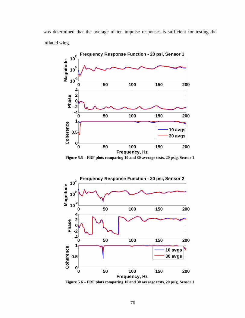
was determined that the average of ten impulse responses is sufficient for testing the
inflated wing.
0 50 100 150 20010
-2
100
102
Mag
nitu
de
Frequency Response Function - 20 psi, Sensor 1
0 50 100 150 200-4-2024
Phas
e
0 50 100 150 2000
0.5
1
Frequency, Hz
Coh
eren
ce
10 avgs30 avgs
Figure 5.5 – FRF plots comparing 10 and 30 average tests, 20 psig, Sensor 1
0 50 100 150 20010
-2
100
102
Mag
nitu
de
Frequency Response Function - 20 psi, Sensor 2
0 50 100 150 200-4-2024
Phas
e
0 50 100 150 2000
0.5
1
Frequency, Hz
Coh
eren
ce 10 avgs30 avgs
Figure 5.6 – FRF plots comparing 10 and 30 average tests, 20 psig, Sensor 1
76

In conducting the test, when driving point measurements were recorded, the bottom of
the wing was struck with the impulse hammer beneath the sensors. With this data,
reciprocity can be examined to evaluate the linearity of the wing response. Figure 5.7
shows the FRF measurements recorded at each measurement point due to an input at the
other measurement point for an internal pressure of 5 psig, while Figure 5.8 shows the
same for an internal pressure of 25 psig. In each of these Figures, the blue plot represents
the accelerometer located at the midpoint of the wing chord and the red plot represents
the accelerometer located near the trailing edge. It can be seen that the FRFs correlate
reasonably well for the 5 psig case at frequencies up to approximately 120 Hz, at which
point the magnitude and phase show slight differences. The coherence, however, shows
distinct differences above 120 Hz.
Figure 5.8 shows that for the case of an internal wing pressure of 25 psig, the
reciprocal FRFs match nearly exactly up to approximately 150 Hz, and reasonably well
from 150 Hz - 200 Hz, the end of the frequency range of interest. This evaluation showed
that reciprocity of the wing response is maintained at all pressures, with only slight
differences at the higher end of the frequency range of interest. Especially for low
pressures, expectations from modal tests of other inflated structures were that reciprocity
would not hold.
77

0 50 100 150 20010
-2
100
102
Mag
nitu
de
Frequency Response Function, 5 psig
0 50 100 150 200-4-2024
Phas
e
0 50 100 150 2000
0.5
1
Frequency, Hz
Coh
eren
ce
Figure 5.7 – FRF plots demonstrating reciprocity, 5 psig
0 50 100 150 20010
-2
100
102
Mag
nitu
de
Frequency Response Function, 25 psig
0 50 100 150 200-4-2024
Phas
e
0 50 100 150 2000
0.5
1
Frequency, Hz
Coh
eren
ce
Figure 5.8 – FRF plots demonstrating reciprocity, 25 psig
78
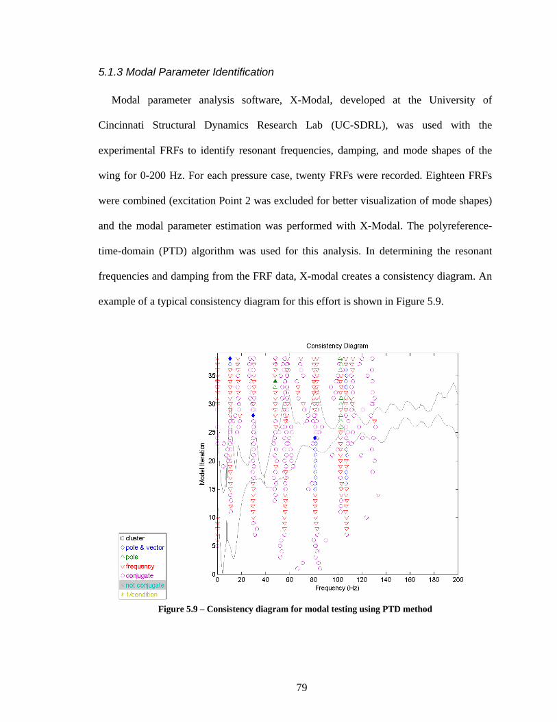
5.1.3 Modal Parameter Identification
Modal parameter analysis software, X-Modal, developed at the University of
Cincinnati Structural Dynamics Research Lab (UC-SDRL), was used with the
experimental FRFs to identify resonant frequencies, damping, and mode shapes of the
wing for 0-200 Hz. For each pressure case, twenty FRFs were recorded. Eighteen FRFs
were combined (excitation Point 2 was excluded for better visualization of mode shapes)
and the modal parameter estimation was performed with X-Modal. The polyreference-
time-domain (PTD) algorithm was used for this analysis. In determining the resonant
frequencies and damping from the FRF data, X-modal creates a consistency diagram. An
example of a typical consistency diagram for this effort is shown in Figure 5.9.
Figure 5.9 – Consistency diagram for modal testing using PTD method
79

In this analysis, four modes of the cantilevered wing were extracted, which include the
first and second bending modes and the first and second torsional modes. Figure 5.10
shows the residue results for a measurement sensor at Point 9 and excitation at Point 3
comparing the PTD results using the estimated modes to the experimental data. Note that
other peak frequencies are seen in the consistency diagram but are not selected for
identification in Figure 5.9. The frequencies and mode shapes for all modes in the
frequency range are included in Table 5.1. The FE model only predicts the first and
second bending and torsion modes of the wing, and does not predict the modes between
which are combination modes including both bending and torsion. Because of this, only
the first and second bending and torsion mode shapes are considered further.
Table 5.1 - Natural frequencies and mode shapes seen in frequency range, 15 psi internal pressure Mode Frequency Description
1 10.6 Hz 1st bending 2 17.3 Hz Combination mode 3 30.0 Hz 1st torsion 4 48.1 Hz 2nd bending 5 58.3 Hz Combination mode 6 71.3 Hz "Tail-flapping" mode 7 81.2 Hz 2nd torsion 8 106.8 Hz High-order combination mode
For inflation at 15 psig, Figure 5.11 shows four mode shapes correlating to the four
bending and torsion frequencies. Note that the mode shapes seen are classical
cantilevered beam first and second bending and first and second torsional modes.
Table 5.2 summarizes the damped resonant frequencies and percent of critical
damping for each of the pressure cases considered. In reviewing these frequencies, it is
seen that for all modes, the frequencies increase with pressure, with the exception of the
second bending mode. The frequency of the second bending mode at 10 psi was 52.8 Hz,
slightly larger than for the 15psi and 20 psi cases, 48.1 Hz and 51.9 Hz, respectively.
80
As seen in Figure 5.9, modal identification is user-dependent. All results herein were
processed in a consistent manner by the author, but as is typical of all modal
identification, some variation in results is expected. In general, however, the identified
frequencies follow expected trends, with the wing stiffening with increased pressure.
Also, note that for all pressure cases, the first torsional mode occurs at a lower frequency
than the second bending mode. The modes are listed out of order of occurrence in Table
5.2 for ease of comparison with FE results.
Note also that high damping percentages were identified for all modes. In each case,
identified damping fell in the range of 4% to 10% modal damping. This is not unexpected
for an inflatable structure.[37]
Table 5.3 lists the undamped natural frequencies of the system. These were calculated
from the damped natural frequencies and damping ratios extracted from the X-Modal
analysis by rearranging and using Equation (5-1). While the difference between the
undamped and damped natural frequencies is not large, the FE models presented below
do not include damping, so it is important to use undamped natural frequencies for model
correlation.
21 ζωω −= nd (5-1)
81

82
Figure 5.10 – Residue results for the FRF at measurement Point 9 and excitation Point 3
Figure 5.11 – Experimentally determined mode shapes, 15 psig internal pressure
a) First bending mode
c) First torsional mode
b) Second bending mode
d) Second torsional mode

83
Table 5.2 – Estimated wing damped natural frequencies and damping 5 psi 10 psi 15 psi 20 psi 25 psi
Mode Frequency/Damping Frequency/Damping Frequency/Damping Frequency/Damping Frequency/Damping1st Bending 9.1 Hz 8.1 % 10.2 Hz 6.9 % 10.7 Hz 6.3 % 11.1 Hz 6.4 % 11.2 Hz 6.7 % 2nd Bending 44.4 Hz 6.1 % 52.8 Hz 5.6 % 48.1 Hz 5.9 % 51.9 Hz 5.7 % 54.8 Hz 4.9 % 1st Torsion 23.6 Hz 9.8 % 28.8 Hz 5.7 % 29.9 Hz 5.5 % 31.8 Hz 5.8 % 33.0 Hz 4.9 % 2nd Torsion 62.5 Hz 7.1 % 76.8 Hz 4.6 % 81.3 Hz 5.2 % 86.5 Hz 6.0 % 91.0 Hz 4.5 %
Table 5.3 – Wing undamped natural frequencies and damping 5 psi 10 psi 15 psi 20 psi 25 psi
Mode Frequency/Damping Frequency/Damping Frequency/Damping Frequency/Damping Frequency/Damping1st Bending 9.1 Hz 8.1 % 10.2 Hz 6.9 % 10.7 Hz 6.3 % 11.1 Hz 6.4 % 11.2 Hz 6.7 % 2nd Bending 44.5 Hz 6.1 % 52.9 Hz 5.6 % 48.2 Hz 5.9 % 52.0 Hz 5.7 % 54.9 Hz 4.9 % 1st Torsion 23.7 Hz 9.8 % 28.8 Hz 5.7 % 29.9 Hz 5.5 % 31.9 Hz 5.8 % 33.0 Hz 4.9 % 2nd Torsion 62.7 Hz 7.1 % 76.9 Hz 4.6 % 81.4 Hz 5.2 % 86.7 Hz 6.0 % 91.1 Hz 4.5 %

5.2 FE Modal Analysis
5.2.1 Model Description and Solution Process
The FE model described in Section 4.2 was used to perform a modal analysis of the
inflatable wing. Mass was not previously included in the model for simulation of static
loadings, but for dynamic response, mass properties are needed. Density for the model
was determined by dividing the weight of the wing by the element volume of the model.
The resulting density used for the analysis was 2.65e-4 lb*s2/in4. Note that the weight of
the wing includes material clamped at the root for wing mounting. This material is not
included in the FE model, so this density is slightly higher than the combined-material
areal density for the wing. Damping was not included in the model.
Two solution processes were considered when conducting the FE modal analysis. In
the first analysis, internal pressure loadings were applied, a static solution was computed
using a linear solver, and a subsequent modal analysis was performed including prestress
effects from the pressure loading. The Block-Lanczos solver in ANSYS was used for the
modal analysis. In this first analysis, only the “effective” linear orthotropic material
model was considered, because inclusion of the nonlinear material model requires the use
of a nonlinear solver.
In the second analysis, a nonlinear solver was used to compute the internal pressure
solution, and a modal analysis was computed using the prestress effects from the internal
pressurization. Again, the modal solution was computed using the Block-Lanczos solver.
Both the “effective” linear orthotropic and the modified nonlinear isotropic material
models were considered using this analysis process.
84
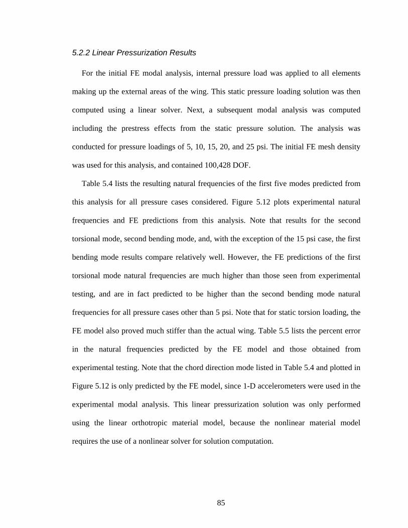
5.2.2 Linear Pressurization Results
For the initial FE modal analysis, internal pressure load was applied to all elements
making up the external areas of the wing. This static pressure loading solution was then
computed using a linear solver. Next, a subsequent modal analysis was computed
including the prestress effects from the static pressure solution. The analysis was
conducted for pressure loadings of 5, 10, 15, 20, and 25 psi. The initial FE mesh density
was used for this analysis, and contained 100,428 DOF.
Table 5.4 lists the resulting natural frequencies of the first five modes predicted from
this analysis for all pressure cases considered. Figure 5.12 plots experimental natural
frequencies and FE predictions from this analysis. Note that results for the second
torsional mode, second bending mode, and, with the exception of the 15 psi case, the first
bending mode results compare relatively well. However, the FE predictions of the first
torsional mode natural frequencies are much higher than those seen from experimental
testing, and are in fact predicted to be higher than the second bending mode natural
frequencies for all pressure cases other than 5 psi. Note that for static torsion loading, the
FE model also proved much stiffer than the actual wing. Table 5.5 lists the percent error
in the natural frequencies predicted by the FE model and those obtained from
experimental testing. Note that the chord direction mode listed in Table 5.4 and plotted in
Figure 5.12 is only predicted by the FE model, since 1-D accelerometers were used in the
experimental modal analysis. This linear pressurization solution was only performed
using the linear orthotropic material model, because the nonlinear material model
requires the use of a nonlinear solver for solution computation.
85

Table 5.4 – FE predictions of wing natural frequencies, linear pressure solution Mode 5 psi 10 psi 15 psi 20 psi 25 psi
1st Bending 13.0 Hz 21.7 Hz 31.0 Hz 20.0 Hz 22.1 Hz *Mode in chord direction 33.1 Hz 34.1 Hz 34.6 Hz 34.8 Hz 35.5 Hz
2nd Bending 49.8 Hz 55.6 Hz 61.1 Hz 63.3 Hz 69.2 Hz 1st Torsion 44.4 Hz 60.2 Hz 70.4 Hz 73.3 Hz 77.2 Hz 2nd Torsion 71.9 Hz 84.6 Hz 94.1 Hz 105.5 Hz 112.2 Hz
Table 5.5 – Percent error from experimental in linearly applied pressure FE resonant frequencies Mode 5 psi 10 psi 15 psi 20 psi 25 psi
1st Bending 42.9% 112.7% 189.7% 80.2% 97.3%2nd Bending 11.9% 5.1% 26.8% 21.7% 26.0%1st Torsion 87.3% 109.0% 135.5% 129.8% 133.9%2nd Torsion 14.7% 10.0% 15.6% 21.7% 23.2%
0 5 10 15 20 25 300
20
40
60
80
100
120
Internal Pressure, psig
Freq
uenc
y, H
z
Linear FEA and X-modal Results
Figure 5.12 – Comparison between estimated wing natural frequencies from experimental modal testing and predicted natural frequencies from FE modal analysis with linear pressurization solution
5.2.3 Nonlinear Pressurization Results
Next, the modal analysis was performed using a nonlinear solver to compute the static
pressure preloading. Internal pressure loading was again applied to the external areas of
86

the wing model, with a nonlinear solver being used to compute this static pressure
solution. The initial FE mesh density was used for this analysis, and contained 100,428
DOF. When including prestress effects from a nonlinear static solution in an ANSYS
modal analysis, the standard commands cannot be used. Instead of using the standard
SOLVE command to perform the modal analysis, the following string of commands must
be used [40].
/SOLU ANTYPE,MODAL PSTRESS,ON MODOPT,LANB,10 MXPAND,10 PSOLVE,EIGLANB FINISH /SOLU EXPASS,ON PSOLVE,EIGEXP FINISH
Table 5.6 lists the resulting natural frequency predictions for the 10 and 15 psi cases,
along with the percent error in the predicted frequencies from those seen in experimental
testing, for a model incorporating the linear orthotropic material model. Higher pressure
loading solutions failed to converge. For all cases, the nonlinear pressurization solution
predicts the experimental natural frequencies more accurately than the linear
pressurization solution. The largest error seen is 40.8%, for the 15 psi first torsion mode,
whereas the linear pressurization solution had an error of 109.0% for this case. It is
interesting to note that for the 10 psi case, the first torsional frequency is under-predicted
by only 1%, but for the 15 psi case, the first torsional frequency is over-predicted by
40.8%. For the 10 psi case, this mode is the most accurately predicted, but for the 15 psi
87

case it is the prediction with the highest error. It is also of note that for the 10 psi case, the
model underpredicts all natural frequencies, indicating a model that is too soft. This is in
contrast to static loading cases, where the model continually proved too stiff.
Finally, the same nonlinear pressurization solution process was used with a model
incorporating the adjusted nonlinear isotropic material model for 10 psi, and these results
along with the percent error from experimental results, are listed in Table 5.7. The
intermediate FE mesh density was used for this analysis, and contained 69,750 DOF.
Note that when compared with the linear orthotropic material model results, the nonlinear
material model more accurately predicts all modes except for the 1st torsion mode. This is
an interesting result, since static loadings were more accurately modeled using the linear
orthotropic material model. The wing mode shapes predicted from this analysis are seen
in Figure 5.13. These mode shapes match those extracted from the experimental modal
analysis shown in Figure 5.11. Only 10 psi results are available using this analysis
process. When this analysis process was implemented with an internal pressure case of 15
psi, the modal analysis did not return natural frequency predictions.
When the results for the two material models are compared for the 10 psi case, the first
and second bending and second torsional frequencies are more accurately predicted by
the adjusted nonlinear material model, and are all predicted to within 10% of the
experimental values. Only the first torsional frequency is more accurately predicted by
the “effective” linear material model, and this is in fact the most accurate prediction out
of all FE cases. It is interesting to note that for static loadings, the “effective” linear
orthotropic material model was more accurate, while here for the modal analysis, the
nonlinear isotropic material model was generally more accurate.
88

Table 5.6 – FE predictions of wing modes and natural frequencies calculated using non-linear pressure solution, linear orthotropic material model
Mode 10 psi 15 psi % Error, 10 psi % Error, 15 psi 1st Bending 9.1 Hz 9.2 Hz -10.8% -14.0% 1st Torsion 28.5 Hz 42.1 Hz -1.0% 40.8%
*Mode in chord direction 32.6 Hz 36.8 Hz N/A N/A 2nd Bending 42.7 Hz 46.3 Hz -19.3% -3.9% 2nd Torsion 69.2 Hz 92.2 Hz -10.0% 13.3%
Table 5.7 – FE predictions of wing modes and natural frequencies calculated using, non-linear pressure solution, nonlinear isotropic material model
Mode FEA 10 psi % Error, 10 psi 1st Bending 9.9 Hz -2.9% 1st Torsion 34.1 Hz 18.4%
*Mode in chord direction 38.7 Hz N/A 2nd Bending 48.0 Hz -9.3% 2nd Torsion 81.5 Hz 6.0%
89

a) First bending mode b) First torsional mode
d) Second torsional mode c) Second bending mode
Figure 5.13 – FE predicted mode shapes using adjusted nonlinear isotropic material model and mesh density of 69,750 DOF
90

CHAPTER 6: SUMMARY
6.1 Detailed Summary
Initial material properties were determined from testing performed by ILC Dover, and
these tests and resulting material properties were presented. Additionally, static testing
was performed on the wing to determine wing response to bending and twisting loads and
provide a means to validate a FE model. Bending tests were performed, and it was found
that nominally equivalent wings respond with wide variation. In addition, responses to
torsion loads at the wing tip were investigated. In all static tests, a high level of hysteresis
was evident in the wing.
A finite element model of an inflatable wing was developed using ANSYS FE
software. Modeling concepts were validated by first creating FE models of inflatable
Vectran cylinders and simulating a shear modulus test. The FE model of the inflatable
wing included nonlinear solutions to internal pressure loading and external force loading.
A two-step analysis procedure was implemented in the wing model, with internal
pressurization being applied in one solution, and a subsequent solution step where
external loadings were applied.
Both linear orthotropic and nonlinear isotropic material models were considered. An
“effective” linear orthotropic material model was found to correlate well to low tip force
bending loads at 10 psi internal pressure, and for tip loads up to 11.24 lbf for internal
pressure of 15 psi. Little difference was seen between resulting bending deflections
between the 10 psi and 15 psi solutions. An adjusted nonlinear isotropic material model
proved stiffer than the “effective” linear orthotropic model for the 10 psi case. However,
when an internal pressure of 15 psi was considered, the resulting bending deflections in
91

the model were actually greater than those seen in laboratory testing. The linear
orthotropic material model showed little difference between two pressure solutions,
underpredicting deflections compared to experimental results. The nonlinear isotropic
material model provided substantially different deflections for different pressures, but
overpredicted deflections compared with 15 psi experimental values.
Mesh density studies were conducted and it was found that when using the nonlinear
isotropic material model, a much more coarse mesh could be used to obtain solutions for
an internal pressure of 10 psi. This mesh resulted in greatly reduced solution times.
Dynamic response of the wing was investigated through an experimental modal
analysis. A standard impact hammer test was conducted with two output accelerometers
and nine input locations. Unexpected results from this experimental test were the clean
FRF’s from an inflatable structure, and the fact that the reciprocity of the system was
good. Previous inflatable programs suggested that neither of these would be true. From
this test, wing natural frequencies and mode shapes were identified.
Two types of FE modal analyses were considered, with one obtaining the pressure
preloading solution using a linear solver, while the second used a nonlinear solver. It was
found that the linear pressurization solution predicted the second bending and second
torsion natural frequencies relatively well, but errors in predicting the first bending and
especially the first torsion mode were much higher. The nonlinear pressurization solution
generally predicted all four natural frequencies, first and second bending and first and
second torsion more accurately, though only low internal pressure solutions converged.
The fundamental frequency of the wing was most accurately predicted using the
92

nonlinear pressurization solution process and the nonlinear isotropic material model, with
and error less than 3%.
6.2 Contributions
Contributions to the community from this work are:
• Static wing response to bending and torsion loads has been documented from
experimental testing
• Natural frequencies and mode shapes of an inflatable wing have been
determined through an experimental modal analysis. Impact hammer testing
was shown to be an effective method for conducting such tests.
• A finite element model of an inflatable wing was created
o Material properties were explored, and reduction factors were
determined and applied to experimental tensile test material data.
o Wing warping forces were modeled qualitatively.
o FE predictions of natural frequencies and mode shapes shows promise
that the model can be used to effectively model dynamic wing
response.
• Overall, the FE modeling processes documented herein provide a valuable
reference for future modeling of inflatable wings.
6.3 Future Work
An area for further studies is adjustment of the FE model to include properties of the
internal bladder. Current material properties are based on the Vectran material only. It
may be possible to develop a hybrid material model that more accurately models the
93

response of the wing. Related to this, testing of other wings constructed of only one layer
of urethane-coated nylon would provide data for a system comparable to the bladder.
Comparisons of the response of such a wing to the Vectran wings would lead to
determining whether the bladder or the Vectran restraint dominates wing response.
An alternative option would be to apply the FE methodology herein to wings
constructed of urethane-coated nylon. This would also lead to a determination of the level
that the bladder dominates the wing response.
Another possible area for future work is conducting tests to determine modulus
properties of the fabric while inflated. Perhaps the reason that the model continually
proves too stiff for static loading is the reliance on material properties of Vectran strips. It
may be that the restraint stiffness does not dominate wing response.
Investigation into other element types that would better model the stress-stiffening
effects of the internal pressurization is also recommended. The current model does not
effectively stiffen with increasing pressure. This could also lead to possible ways to
include hysteresis and creep in the model.
Other forms of wing warping in addition to modeling servo moments could also be
considered. Modeling wing response to application of smart materials would be
beneficial, though work to increase the model’s accuracy is recommended first.
94

APPENDIX A: ANSYS BATCH FILE COMMANDS
The following batch commands were used to create the finite element model of the
inflatable wing. Three material models are included. For linear orthotropic material
properties, the parameters defined at the beginning of the file are used. Nonlinear
isotropic material models are also included, but as printed are commented out. To use
either nonlinear material model, the comments from that section must be removed and the
linear orthotropic section should be commented out. Commands for three mesh densities
are included, with the two coarser meshes currently commented out. When changing the
mesh density, the load application nodes must also be changed, and these changes are
also included as comments. Three solution files are included, separated below by lines of
“#######,” and each is clearly labeled at the beginning.
Also included is a sample batch input file for simulating wing warping. This file
begins on Page 107.
! This file creates the geometry and mesh for the inflatable wing model. /filname, FILENAME /prep7 ! define parameters e_fill= 1.22e6*.08 e_warp= 1.36e6*.08 shear_mod= 20e3 int_press= 10 tip_load= 2.2481 ! change view for interactive mode /VIEW,1,1 ! create root keypoints K, 1, 0.000000, -0.5595000, 8.500500, K, 2, 0.000000, 0.9758637E-01, 8.100849,
95

K, 3, 0.000000, -1.296945, 7.821943, K, 4, 0.000000, 0.5779612, 7.401153, K, 5, 0.000000, -1.471254, 6.991310, K, 6, 0.000000, 1.033980, 6.337101, K, 7, 0.000000, -1.538836, 5.970979, K, 8, 0.000000, 1.346173, 5.036847, K, 9, 0.000000, -1.552504, 4.796735, K,10, 0.000000, 1.444189, 3.545226, K,11, 0.000000, -1.491011, 3.460233, K,12, 0.000000, 1.407859, 1.817772, K,13, 0.000000, -1.416350, 1.829688, K,14, 0.000000, 1.294533, 0.1071999, K,15, 0.000000, -1.354123, 0.1718821, K,16, 0.000000, 1.096033, -1.502466, K,17, 0.000000, -1.254139, -1.418965, K,18, 0.000000, 0.8318012, -3.047054, K,19, 0.000000, -1.127290, -2.946888, K,20, 0.000000, 0.5584566, -4.482636, K,21, 0.000000, -1.022033, -4.381605, K,22, 0.000000, 0.2928351, -5.730581, K,23, 0.000000, -0.9289871, -5.642207, K,24, 0.000000, 0.1400362E-01, -6.823949, K,25, 0.000000, -0.8221342, -6.755400, K,26, 0.000000, -0.2273438, -7.744520, K,27, 0.000000, -0.7510242, -7.692574, K,28, 0.000000, -0.5235000, -8.500500, K,29, 0.000000, -0.1749602, 8.392741, K,30, 0.000000, 0.4109251, 7.801201, K,31, 0.000000, 0.9285751, 6.921547, K,32, 0.000000, 1.340398, 5.723125, K,33, 0.000000, 1.577005, 4.302984, K,34, 0.000000, 1.667131, 2.676428, K,35, 0.000000, 1.597981, 0.9461363, K,36, 0.000000, 1.433291, -0.7269837, K,37, 0.000000, 1.214384, -2.317608, K,38, 0.000000, 0.9521861, -3.813790, K,39, 0.000000, 0.6656415, -5.157691, K,40, 0.000000, 0.3926820, -6.338282, K,41, 0.000000, 0.1293430, -7.346110, K,42, 0.000000, -0.1175397, -8.223535, K,43, 0.000000, -0.9431758, -8.182687, K,44, 0.000000, -1.021820, -7.241836, K,45, 0.000000, -1.115986, -6.221881, K,46, 0.000000, -1.214917, -5.029577, K,47, 0.000000, -1.326415, -3.682717, K,48, 0.000000, -1.431923, -2.202952,
96

K,49, 0.000000, -1.534564, -0.6380242, K,50, 0.000000, -1.615368, 0.9921470, K,51, 0.000000, -1.666754, 2.635204, K,52, 0.000000, -1.665784, 4.121857, K,53, 0.000000, -1.663397, 5.385171, K,54, 0.000000, -1.607600, 6.488050, K,55, 0.000000, -1.470940, 7.424868, K,56, 0.000000, -1.060565, 8.305049, ! create root lines LARC, 1, 2, 29 LARC, 2, 4, 30 LARC, 4, 6, 31 LARC, 6, 8, 32 LARC, 8, 10, 33 LARC, 10, 12, 34 LARC, 12, 14, 35 LARC, 14, 16, 36 LARC, 16, 18, 37 LARC, 18, 20, 38 LARC, 20, 22, 39 LARC, 22, 24, 40 LARC, 24, 26, 41 LARC, 26, 28, 42 LARC, 28, 27, 43 LARC, 27, 25, 44 LARC, 25, 23, 45 LARC, 23, 21, 46 LARC, 21, 19, 47 LARC, 19, 17, 48 LARC, 17, 15, 49 LARC, 15, 13, 50 LARC, 13, 11, 51 LARC, 11, 9, 52 LARC, 9, 7, 53 LARC, 7, 5, 54 LARC, 5, 3, 55 LARC, 3, 1, 56 ! create component of constrained lines CM,l_root_constr,LINE ! create spar lines LSTR, 2, 3 LSTR, 4, 5 LSTR, 6, 7
97

LSTR, 8, 9 LSTR, 10, 11 LSTR, 12, 13 LSTR, 14, 15 LSTR, 16, 17 LSTR, 18, 19 LSTR, 20, 21 LSTR, 22, 23 LSTR, 24, 25 LSTR, 26, 27 ! create component of all root lines CM,l_root,LINE ! create tip profile by scaling down root lines LSSCALE,all,,,.65,.65,.65,,0,0 ! unselect root lines CMSEL,U,l_root ! move tip profile to proper location LGEN,,all,,,36,0,0,,,1 CM,l_tip,LINE ALLSEL,all ! create restraint/spar lines LSTR, 1, 57 LSTR, 2, 58 LSTR, 4, 59 LSTR, 6, 60 LSTR, 8, 61 LSTR, 10, 62 LSTR, 12, 63 LSTR, 14, 64 LSTR, 16, 65 LSTR, 18, 66 LSTR, 20, 67 LSTR, 22, 68 LSTR, 24, 69 LSTR, 26, 70 LSTR, 28, 71 LSTR, 27, 72 LSTR, 25, 73 LSTR, 23, 74
98

LSTR, 21, 75 LSTR, 19, 76 LSTR, 17, 77 LSTR, 15, 78 LSTR, 13, 79 LSTR, 11, 80 LSTR, 9, 81 LSTR, 7, 82 LSTR, 5, 83 LSTR, 3, 84 ! create restraint areas AL, 1, 84, 42, 83 AL, 2, 85, 43, 84 AL, 3, 86, 44, 85 AL, 4, 87, 45, 86 AL, 5, 88, 46, 87 AL, 6, 89, 47, 88 AL, 7, 90, 48, 89 AL, 8, 91, 49, 90 AL, 9, 92, 50, 91 AL, 10, 93, 51, 92 AL, 11, 94, 52, 93 AL, 12, 95, 53, 94 AL, 13, 96, 54, 95 AL, 14, 97, 55, 96 AL, 15, 98, 56, 97 AL, 16, 99, 57, 98 AL, 17, 100, 58, 99 AL, 18, 101, 59, 100 AL, 19, 102, 60, 101 AL, 20, 103, 61, 102 AL, 21, 104, 62, 103 AL, 22, 105, 63, 104 AL, 23, 106, 64, 105 AL, 24, 107, 65, 106 AL, 25, 108, 66, 107 AL, 26, 109, 67, 108 AL, 27, 110, 68, 109 AL, 28, 83, 69, 110 ! create spar areas AL, 29, 84, 70, 110 AL, 30, 85, 71, 109 AL, 31, 86, 72, 108 AL, 32, 87, 73, 107
99

AL, 33, 88, 74, 106 AL, 34, 89, 75, 105 AL, 35, 90, 76, 104 AL, 36, 91, 77, 103 AL, 37, 92, 78, 102 AL, 38, 93, 79, 101 AL, 39, 94, 80, 100 AL, 40, 95, 81, 99 AL, 41, 96, 82, 98 ! create keypoints for tip spline KL, 70, .5,, KL, 71, .5,, KL, 72, .5,, KL, 73, .5,, KL, 74, .5,, KL, 75, .5,, KL, 76, .5,, KL, 77, .5,, KL, 78, .5,, KL, 79, .5,, KL, 80, .5,, KL, 81, .5,, KL, 82, .5,, ! create tip spline KSEL,S,KP,,57 KSEL,A,KP,,71 KSEL,A,KP,,86,97,1 BSPLIN,all, ALLSEL,all ! create wing tip areas LSEL,S,LINE,,42,55,1 LSEL,A,LINE,,111 AL,all LSEL,S,LINE,,56,69,1 LSEL,A,LINE,,111 AL,all ALLSEL, all
100

! create components !wing endcap ASEL,S,AREA,,42,43,1 CM,a_endcap,AREA !wing restraint ASEL,S,AREA,,1,28,1 CM,a_restraint,AREA !internal spars ASEL,S,AREA,,29,41,1 CM,a_spars,AREA !endseam line LSEL,S,LINE,,111 CM,l_endseam,LINE !lines at wing tip CMSEL,S,l_tip CMSEL,A,l_endseam CM,l_tip,LINE ! Reverse area normals CMSEL,S,a_endcap CMSEL,A,a_restraint AREVERSE,all,0 ALLSEL, all ! Define Element type and real constants ET,1,SHELL181 R,1,.013,,,,,, RMORE,,,,,,, ! define linear orthotropic material properties MPTEMP,,,,,,,, MPTEMP,1,0 MPDATA,EX,1,,e_warp MPDATA,EY,1,,e_fill MPDATA,EZ,1,,e_fill MPDATA,PRXY,1,, MPDATA,PRYZ,1,, MPDATA,PRXZ,1,, MPDATA,GXY,1,,shear_mod MPDATA,GYZ,1,,shear_mod
101

MPDATA,GXZ,1,,shear_mod ! define nonlinear isotropic material properties (100% of testing) ! MPTEMP,,,,,,,, ! MPTEMP,1,0 ! MPDATA,EX,1,,e_fill ! *CREATE,file1.UNIA ! 0 0 ! 0.058268908 2915 ! 0.072320662 5375 ! 0.086177696 11990 ! 0.122217633 39550 ! *END ! TBFT,EADD,1,UNIA,file1.UNIA ! /DELETE,file1.UNIA ! TBFT,FADD,1,HYPER,MOON,3 ! TBFT,SOLVE,1,HYPER,MOON,3,1 ! TBFT,FSET,1,HYPER,MOON,3 ! define nonlinear isotropic material properties (75% of testing) ! MPTEMP,,,,,,,, ! MPTEMP,1,0 ! MPDATA,EX,1,,e_fill ! *CREATE,file1.UNIA ! 0 0 ! 0.058268908 2186.25 ! 0.072320662 4031.25 ! 0.086177696 8992.5 ! 0.122217633 29662.5 ! *END ! TBFT,EADD,1,UNIA,file1.UNIA ! /DELETE,file1.UNIA ! TBFT,FADD,1,HYPER,MOON,3 ! TBFT,SOLVE,1,HYPER,MOON,3,1 ! TBFT,FSET,1,HYPER,MOON,3 ! Set mesh sizing for warp direction CMSEL,U,L_ROOT CMSEL,U,L_TIP LESIZE,all,,,72,0.5,1,,,0 ! original mesh ! LESIZE,all,,,50,.5,1 , , ,0 !coarse mesh ! LESIZE,all,,,25,.5,1 , , ,0 !reduced solution time mesh ALLSEL,ALL
102

! mesh restraint and spars CMSEL,U,A_ENDCAP amesh, all ! mesh endcap CMSEL,S,l_endseam LESIZE,all, , ,70,.5,1 , , ,0 ! original mesh ! LESIZE,all, , ,50,.5,1 , , ,0 ! coarse mesh ! LESIZE,all, , ,30,.5,1 , , ,0 ! reduced solution time mesh ALLSEL,ALL CMSEL,S,A_ENDCAP amesh, all ALLSEL, ALL ! create bending tip force component on bottom NSEL,S,NODE,,9053 ! original mesh ! NSEL,S,NODE,,6326 ! coarse mesh ! NSEL,S,NODE,,3227 ! reduced solution time mesh CM,n_tip_load_up,NODE ALLSEL,ALL ! Save database as certain filename SAVE !###################################################### ! Solution commands for bending loads ! set solution options /SOLU NLGEOM,ON NSUBST,1000,7500,150 LNSRCH,ON ! OUTRES,ERASE ! OUTRES,ALL,10 ! apply constraints on root CMSEL,S,l_root_constr DL,all, ,ALL, ! apply internal pressure CMSEL,S,a_restraint
103

CMSEL,A,a_endcap SFA,all,1,PRES,int_press ALLSEL,ALL SSTIF,ON SOLVE ! apply tip load CMSEL,S,n_tip_load_up F,all,FY,tip_load ALLSEL,ALL SSTIF,ON SOLVE FINISH !/exit, nosave !###################################################### ! Solution commands for linear pressurization modal analysis ! assign results file ! /ASSIGN,RST, ! set solution options /SOLU ! apply constraints on root CMSEL,S,l_root_constr DL,all, ,ALL, ! apply internal pressure CMSEL,S,a_restraint CMSEL,A,a_endcap SFA,all,1,PRES,int_press ALLSEL,ALL PSTRES,ON SOLVE FINISH
104

/SOLU ANTYPE,MODAL MODOPT,LANB,10 PSTRES,ON SOLVE FINISH !/exit, nosave !###################################################### ! Solution commands for nonlinear pressurization modal analysis ! set solution options /SOLU NLGEOM,ON NSUBST,1500,10000,150 LNSRCH,ON ! OUTRES,ERASE ! OUTRES,ALL,25 PSTRESS,ON ! apply constraints on root CMSEL,S,l_root_constr DL,all, ,ALL,
105

! apply internal pressure CMSEL,S,a_restraint CMSEL,A,a_endcap SFA,all,1,PRES,int_press ALLSEL,ALL SOLVE FINISH /SOLU ANTYPE,MODAL PSTRESS,ON MODOPT,LANB,10 MXPAND,10 PSOLVE,EIGLANB FINISH /SOLU EXPASS,ON PSOLVE,EIGEXP FINISH !/exit, nosave
106

! The following file creates and solves the FE model of the FASM wing with applied wing warping forces. /filname, warp_1 /prep7 ! define parameters int_press= 10 warp_mom= 8 ! change view for interactive mode /VIEW,1,1 ! create root keypoints K, 1, 0.000000, -0.5595000, 8.500500, K, 2, 0.000000, 0.9758637E-01, 8.100849, K, 3, 0.000000, -1.296945, 7.821943, K, 4, 0.000000, 0.5779612, 7.401153, K, 5, 0.000000, -1.471254, 6.991310, K, 6, 0.000000, 1.033980, 6.337101, K, 7, 0.000000, -1.538836, 5.970979, K, 8, 0.000000, 1.346173, 5.036847, K, 9, 0.000000, -1.552504, 4.796735, K,10, 0.000000, 1.444189, 3.545226, K,11, 0.000000, -1.491011, 3.460233, K,12, 0.000000, 1.407859, 1.817772, K,13, 0.000000, -1.416350, 1.829688, K,14, 0.000000, 1.294533, 0.1071999, K,15, 0.000000, -1.354123, 0.1718821, K,16, 0.000000, 1.096033, -1.502466, K,17, 0.000000, -1.254139, -1.418965, K,18, 0.000000, 0.8318012, -3.047054, K,19, 0.000000, -1.127290, -2.946888, K,20, 0.000000, 0.5584566, -4.482636, K,21, 0.000000, -1.022033, -4.381605, K,22, 0.000000, 0.2928351, -5.730581, K,23, 0.000000, -0.9289871, -5.642207, K,24, 0.000000, 0.1400362E-01, -6.823949, K,25, 0.000000, -0.8221342, -6.755400, K,26, 0.000000, -0.2273438, -7.744520, K,27, 0.000000, -0.7510242, -7.692574, K,28, 0.000000, -0.5235000, -8.500500, K,29, 0.000000, -0.1749602, 8.392741, K,30, 0.000000, 0.4109251, 7.801201, K,31, 0.000000, 0.9285751, 6.921547, K,32, 0.000000, 1.340398, 5.723125,
107

K,33, 0.000000, 1.577005, 4.302984, K,34, 0.000000, 1.667131, 2.676428, K,35, 0.000000, 1.597981, 0.9461363, K,36, 0.000000, 1.433291, -0.7269837, K,37, 0.000000, 1.214384, -2.317608, K,38, 0.000000, 0.9521861, -3.813790, K,39, 0.000000, 0.6656415, -5.157691, K,40, 0.000000, 0.3926820, -6.338282, K,41, 0.000000, 0.1293430, -7.346110, K,42, 0.000000, -0.1175397, -8.223535, K,43, 0.000000, -0.9431758, -8.182687, K,44, 0.000000, -1.021820, -7.241836, K,45, 0.000000, -1.115986, -6.221881, K,46, 0.000000, -1.214917, -5.029577, K,47, 0.000000, -1.326415, -3.682717, K,48, 0.000000, -1.431923, -2.202952, K,49, 0.000000, -1.534564, -0.6380242, K,50, 0.000000, -1.615368, 0.9921470, K,51, 0.000000, -1.666754, 2.635204, K,52, 0.000000, -1.665784, 4.121857, K,53, 0.000000, -1.663397, 5.385171, K,54, 0.000000, -1.607600, 6.488050, K,55, 0.000000, -1.470940, 7.424868, K,56, 0.000000, -1.060565, 8.305049, ! create root lines LARC, 1, 2, 29 LARC, 2, 4, 30 LARC, 4, 6, 31 LARC, 6, 8, 32 LARC, 8, 10, 33 LARC, 10, 12, 34 LARC, 12, 14, 35 LARC, 14, 16, 36 LARC, 16, 18, 37 LARC, 18, 20, 38 LARC, 20, 22, 39 LARC, 22, 24, 40 LARC, 24, 26, 41 LARC, 26, 28, 42 LARC, 28, 27, 43 LARC, 27, 25, 44 LARC, 25, 23, 45 LARC, 23, 21, 46 LARC, 21, 19, 47 LARC, 19, 17, 48
108

LARC, 17, 15, 49 LARC, 15, 13, 50 LARC, 13, 11, 51 LARC, 11, 9, 52 LARC, 9, 7, 53 LARC, 7, 5, 54 LARC, 5, 3, 55 LARC, 3, 1, 56 ! create component of constrained lines CM,l_root_constr,LINE ! create spar lines LSTR, 2, 3 LSTR, 4, 5 LSTR, 6, 7 LSTR, 8, 9 LSTR, 10, 11 LSTR, 12, 13 LSTR, 14, 15 LSTR, 16, 17 LSTR, 18, 19 LSTR, 20, 21 LSTR, 22, 23 LSTR, 24, 25 LSTR, 26, 27 ! create component of all root lines CM,l_root,LINE ! create tip profile by scaling down root lines LSSCALE,all,,,.65,.65,.65,,0,0 ! unselect root lines CMSEL,U,l_root ! move tip profile to proper location LGEN,,all,,,36,0,0,,,1 CM,l_tip,LINE ALLSEL,all ! create restraint/spar lines LSTR, 1, 57 LSTR, 2, 58
109

LSTR, 4, 59 LSTR, 6, 60 LSTR, 8, 61 LSTR, 10, 62 LSTR, 12, 63 LSTR, 14, 64 LSTR, 16, 65 LSTR, 18, 66 LSTR, 20, 67 LSTR, 22, 68 LSTR, 24, 69 LSTR, 26, 70 LSTR, 28, 71 LSTR, 27, 72 LSTR, 25, 73 LSTR, 23, 74 LSTR, 21, 75 LSTR, 19, 76 LSTR, 17, 77 LSTR, 15, 78 LSTR, 13, 79 LSTR, 11, 80 LSTR, 9, 81 LSTR, 7, 82 LSTR, 5, 83 LSTR, 3, 84 ! create restraint areas AL, 1, 84, 42, 83 AL, 2, 85, 43, 84 AL, 3, 86, 44, 85 AL, 4, 87, 45, 86 AL, 5, 88, 46, 87 AL, 6, 89, 47, 88 AL, 7, 90, 48, 89 AL, 8, 91, 49, 90 AL, 9, 92, 50, 91 AL, 10, 93, 51, 92 AL, 11, 94, 52, 93 AL, 12, 95, 53, 94 AL, 13, 96, 54, 95 AL, 14, 97, 55, 96 AL, 15, 98, 56, 97 AL, 16, 99, 57, 98 AL, 17, 100, 58, 99 AL, 18, 101, 59, 100
110

AL, 19, 102, 60, 101 AL, 20, 103, 61, 102 AL, 21, 104, 62, 103 AL, 22, 105, 63, 104 AL, 23, 106, 64, 105 AL, 24, 107, 65, 106 AL, 25, 108, 66, 107 AL, 26, 109, 67, 108 AL, 27, 110, 68, 109 AL, 28, 83, 69, 110 ! create spar areas AL, 29, 84, 70, 110 AL, 30, 85, 71, 109 AL, 31, 86, 72, 108 AL, 32, 87, 73, 107 AL, 33, 88, 74, 106 AL, 34, 89, 75, 105 AL, 35, 90, 76, 104 AL, 36, 91, 77, 103 AL, 37, 92, 78, 102 AL, 38, 93, 79, 101 AL, 39, 94, 80, 100 AL, 40, 95, 81, 99 AL, 41, 96, 82, 98 ! create keypoints for tip spline KL, 70, .5,, KL, 71, .5,, KL, 72, .5,, KL, 73, .5,, KL, 74, .5,, KL, 75, .5,, KL, 76, .5,, KL, 77, .5,, KL, 78, .5,, KL, 79, .5,, KL, 80, .5,, KL, 81, .5,, KL, 82, .5,, ! create tip spline KSEL,S,KP,,57 KSEL,A,KP,,71
111

KSEL,A,KP,,86,97,1 BSPLIN,all, ALLSEL,all ! create wing tip areas LSEL,S,LINE,,42,55,1 LSEL,A,LINE,,111 AL,all LSEL,S,LINE,,56,69,1 LSEL,A,LINE,,111 AL,all ALLSEL, all ! create components !a_endcap ASEL,S,AREA,,42,43,1 CM,a_endcap,AREA !A_RESTRAINT ASEL,S,AREA,,1,28,1 CM,a_restraint,AREA !A_SPARS ASEL,S,AREA,,29,41,1 CM,a_spars,AREA !L_ENDSEAM LSEL,S,LINE,,111 CM,l_endseam,LINE !L_TIP CMSEL,S,l_tip CMSEL,A,l_endseam CM,l_tip,LINE ! Reverse area normals CMSEL,S,a_endcap CMSEL,A,a_restraint AREVERSE,all,0 ALLSEL, all
112

! Define Element type and real constants ET,1,SHELL181 R,1,.013,,,,,, RMORE,,,,,,, ! define material properties *CREATE,file1.UNIA 0 0 0.058268908 2915 0.072320662 5375 0.086177696 11990 0.122217633 39550 *END TBFT,EADD,1,UNIA,file1.UNIA /DELETE,file1.UNIA TBFT,FADD,1,HYPER,MOON,3 TBFT,SOLVE,1,HYPER,MOON,3,1 TBFT,FSET,1,HYPER,MOON,3 ! Set mesh sizing for warp direction CMSEL,U,L_ROOT CMSEL,U,L_TIP LESIZE,all,,,25,0.5,1,,,0 ALLSEL,ALL ! mesh CMSEL,U,A_ENDCAP amesh, all ! mesh endcap CMSEL,S,l_endseam LESIZE,all, , ,30,.5,1 , , ,0 ALLSEL,ALL CMSEL,S,A_ENDCAP amesh, all !create "servo" patches !patch 1 NSEL,S,NODE,,1977 NSEL,A,NODE,,2010 NSEL,A,NODE,,2011 NSEL,A,NODE,,2237 NSEL,A,NODE,,2238 NSEL,A,NODE,,2239
113

NSEL,A,NODE,,2240 NSEL,A,NODE,,2241 NSEL,A,NODE,,2242 NSEL,A,NODE,,2243 NSEL,A,NODE,,2244 NSEL,A,NODE,,2268 NSEL,A,NODE,,2269 NSEL,A,NODE,,2431 NSEL,A,NODE,,2432 NSEL,A,NODE,,2433 NSEL,A,NODE,,2434 NSEL,A,NODE,,2435 NSEL,A,NODE,,2436 NSEL,A,NODE,,2437 NSEL,A,NODE,,2438 NSEL,A,NODE,,2439 NSEL,A,NODE,,2440 NSEL,A,NODE,,2441 NSEL,A,NODE,,2442 NSEL,A,NODE,,2443 NSEL,A,NODE,,2444 NSEL,A,NODE,,2445 NSEL,A,NODE,,2446 NSEL,A,NODE,,2447 NSEL,A,NODE,,2448 NSEL,A,NODE,,2449 NSEL,A,NODE,,2450 NSEL,A,NODE,,2451 NSEL,A,NODE,,2475 NSEL,A,NODE,,2476 NSEL,A,NODE,,2615 NSEL,A,NODE,,2616 NSEL,A,NODE,,2617 NSEL,A,NODE,,2618 NSEL,A,NODE,,2619 NSEL,A,NODE,,2620 NSEL,A,NODE,,2621 NSEL,A,NODE,,2622 NSEL,A,NODE,,2623 NSEL,A,NODE,,2624 NSEL,A,NODE,,2625 NSEL,A,NODE,,2626 CM,patch_1,NODE ALLSEL, ALL
114

!patch 2 NSEL,S,NODE,,2005 NSEL,A,NODE,,2006 NSEL,A,NODE,,2007 NSEL,A,NODE,,2263 NSEL,A,NODE,,2264 NSEL,A,NODE,,2265 NSEL,A,NODE,,2396 NSEL,A,NODE,,2397 NSEL,A,NODE,,2398 NSEL,A,NODE,,2399 NSEL,A,NODE,,2400 NSEL,A,NODE,,2401 NSEL,A,NODE,,2402 NSEL,A,NODE,,2403 NSEL,A,NODE,,2404 NSEL,A,NODE,,2405 NSEL,A,NODE,,2406 NSEL,A,NODE,,2407 NSEL,A,NODE,,2408 NSEL,A,NODE,,2409 NSEL,A,NODE,,2410 NSEL,A,NODE,,2411 NSEL,A,NODE,,2412 NSEL,A,NODE,,2413 NSEL,A,NODE,,2414 NSEL,A,NODE,,2415 NSEL,A,NODE,,2416 NSEL,A,NODE,,2470 NSEL,A,NODE,,2471 NSEL,A,NODE,,2472 NSEL,A,NODE,,2585 NSEL,A,NODE,,2586 NSEL,A,NODE,,2587 NSEL,A,NODE,,2588 NSEL,A,NODE,,2589 NSEL,A,NODE,,2590 NSEL,A,NODE,,2591 NSEL,A,NODE,,2592 NSEL,A,NODE,,2593 NSEL,A,NODE,,2594 NSEL,A,NODE,,2595 NSEL,A,NODE,,2596 NSEL,A,NODE,,2597 NSEL,A,NODE,,2598
115

NSEL,A,NODE,,2599 NSEL,A,NODE,,2600 NSEL,A,NODE,,2601 NSEL,A,NODE,,2602 CM,patch_2,NODE ALLSEL, ALL !patch 3
NSEL,S,NODE,,2000 NSEL,A,NODE,,2001 NSEL,A,NODE,,2002 NSEL,A,NODE,,2258 NSEL,A,NODE,,2259 NSEL,A,NODE,,2260 NSEL,A,NODE,,2361 NSEL,A,NODE,,2362 NSEL,A,NODE,,2363 NSEL,A,NODE,,2364 NSEL,A,NODE,,2365 NSEL,A,NODE,,2366 NSEL,A,NODE,,2367 NSEL,A,NODE,,2368 NSEL,A,NODE,,2369 NSEL,A,NODE,,2370 NSEL,A,NODE,,2371 NSEL,A,NODE,,2372 NSEL,A,NODE,,2373 NSEL,A,NODE,,2374 NSEL,A,NODE,,2375 NSEL,A,NODE,,2376 NSEL,A,NODE,,2377 NSEL,A,NODE,,2378 NSEL,A,NODE,,2379 NSEL,A,NODE,,2380 NSEL,A,NODE,,2381 NSEL,A,NODE,,2465 NSEL,A,NODE,,2466 NSEL,A,NODE,,2467 NSEL,A,NODE,,2555 NSEL,A,NODE,,2556 NSEL,A,NODE,,2557 NSEL,A,NODE,,2558 NSEL,A,NODE,,2559 NSEL,A,NODE,,2560
116

NSEL,A,NODE,,2561 NSEL,A,NODE,,2562 NSEL,A,NODE,,2563 NSEL,A,NODE,,2564 NSEL,A,NODE,,2565 NSEL,A,NODE,,2566 NSEL,A,NODE,,2567 NSEL,A,NODE,,2568 NSEL,A,NODE,,2569 NSEL,A,NODE,,2570 NSEL,A,NODE,,2571 NSEL,A,NODE,,2572 CM,patch_3,NODE ALLSEL, ALL ! create tip force component on bottom NSEL,S,NODE,,3227 CM,n_tip_load_up,NODE ALLSEL,ALL ! Save database SAVE !###################################################### ! Solution ! set solution options /SOLU NLGEOM,ON NSUBST,2000,20000,300 LNSRCH,ON ! apply constraints on root CMSEL,S,l_root_constr DL,all,,ALL, ! apply internal pressure CMSEL,S,a_restraint CMSEL,A,a_endcap SFA,all,1,PRES,int_press ALLSEL,ALL
117

SSTIF,ON SOLVE SAVE,nonlin_matl_10psi_soln,db !! apply patch 1 load CMSEL,S,patch_1 F,all,MX,-warp_mom/48 ALLSEL,ALL !! apply patch 1 load ! CMSEL,S,patch_2 ! F,all,MX,-warp_mom/48 ! ALLSEL,ALL !! apply patch 1 load ! CMSEL,S,patch_3 ! F,all,MX,-warp_mom/48 ! ALLSEL,ALL SSTIF,ON SOLVE FINISH !/exit, nosave
118

APPENDIX B: ADDITIONAL EXPERIMENTAL TEST DATA
This appendix includes experimental data of multiple wings. Each wing is labeled by
its serial number.
Bending Data, Internal pressure of 10 psi:
119
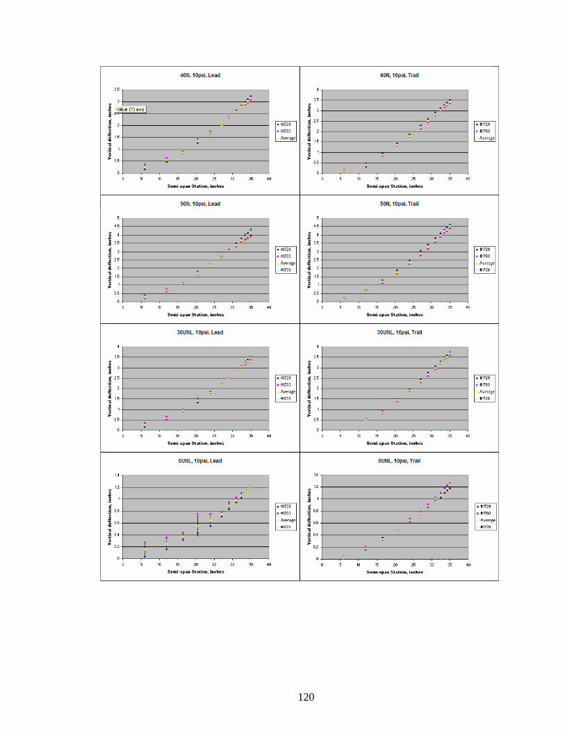
120

Bending Data, Internal pressure of 15 psi:
121

122

Bending Data, Internal pressure of 20 psi:
123

124

Torsion Data, Internal pressure of 10 psi:
125

126

Torsion Data, Internal pressure of 15 psi:
127

128

Torsion Data, Internal pressure of 20 psi:
129

130

REFERENCES
1. 2007 Worldwide UAV Roundup, in Supplement to Aerospace America. 2007.
2. Jacob, J.D., A.D. Simpson, and S. Smith, Design and Flight Testing of Inflatable Wings with Wing Warping. SAE Transactions Journal of Aerospace, 2005: p. pp. 1306-1315.
3. Simpson, A., A. Santhanakrishnan, J. Jacob, and S. Smith, Flying on Air: UAV Flight Testing with Inflatable Wing Technology, in 3rd “Unmanned Unlimited” Technical Conference, Workshop and Exhibit. 2004, AIAA: Chicago, Illinois.
4. Murray, J., et al., Ground and Flight Evaluation of a Small-Scale Inflatable-Winged Aircraft, in 40th Aerospace Sciences Meeting & Exhibit. 2002, AIAA: Reno, NV.
5. Cadogan, D., T. Smith, F. Uhelsky, M. MacKusick, Morphing Inflatable Wing Development for Compact Package Unmanned Aerial Vehicles, in 45th AIAA/ASME/ASCE/AHS/ASC Structures, Structural Dynamics and Materials Conference. 2004, AIAA: Palm Springs, California.
6. Simpson, A., M. Usui, S. Smith, and J.D. Jacob, Aeromechanics of Inflatable Wings, in AIAA 34th Fluid Dynamics Conference. 2004, AIAA: Portland, OR.
7. Simpson, A.D., M. Usui, S.W. Smith, J.D. Jacob, Development and Flight Testing of a UAV with Inflatable-Rigidizable Wings, in 42nd AIAA Aerospace Sciences Meeting and Exhibit. 2004, AIAA: Reno, NV.
8. Cadogan, D., T. Smith, R. Lee, S. Scarborough, D. Graziosi, Inflatable and Rigidizable Wing Components for Unmanned Aerial Vehicles, in 44th AIAA/ASME/ASCE/AHS/ASC Structures, Structural Dynamics and Materials Conference. 2003, AIAA Norfolk, VA.
9. Allred, R., A. Hoyt, L. Harrah, P. McElroy, S. Scarborough, D. Cadogan, Light Curing Rigidizable Inflatable Wing, in 45th AIAA/ASME/ASCE/AHS/ASC Structures, Structural Dynamics and Materials Conference. 2004, AIAA: Palm Springs, CA.
10. Smith, S.C., et. al., The Design of the Canyon Flyer, an Airplane for Mars Exploration, in 42nd AIAA Aerospace Sciences Meeting and Exhibit. 2000, AIAA: Reno NV.
11. Robotic Access to Planetary Surfaces, NASA Science Mission Directorate.
12. Kearns, J., M. Usui, S. Smith, S. Scarborough, T. Smith, D. Cadogan, Development of UV-Curable Inflatable Wings for Low Density Flight Applications, in 5th AIAA Gossamer Spacecraft Forum. 2004, AIAA: Palm Springs, CA.
131
13. Smith, S.W., J.D. Jacob, R. Jones, S. Scarborough and D. Cadogan, A High-Altitude Test of Inflatable Wings for Low-Density Flight Applications, in 7th AIAA Gossamer Spacecraft Forum. 2006, AIAA: Newport, RI.
14. Usui, M., J.D. Jacob, S.W. Smith, S. Scarborough and D. Cadogan, Second Generation Inflatable/RigidizableWings for Low-Density Applications, in 6th AIAA Gossamer Spacecraft Forum. 2005, AIAA: Austin, TX.
15. Usui, M., Design of Inflatable-Rigidizable Wings for Low-Density Flight Applications, in Dept. of Mechanical Engineering. 2004, University of Kentucky: Lexington, KY.
16. http://www.nasm.si.edu/research/aero/aircraft/goodyear_xao.htm.
17. http://www.ilcdover.com/products/aerospace_defense/uavwings.htm.
18. Cadogan, D., et al., Recent Development and Test of Inflatable Wings, in AIAA SDM Conference. 2006, AIAA: Newport, Rhode Island.
19. Jacob, J.D., S.W. Smith, D. Cadogan and S. Scarborough, Expanding the Small UAV Design Space with Inflatable Wings, in SAE AeroTech Congress and Exhibition. 2007, SAE: Los Angeles, CA.
20. Jacob, J.D., S.W. Smith, D. Cadogan and S. Scarborough, Inflatable Wings as a UAV Design Alternative, in AUVSI Unmanned Systems North America 2007. 2007: Washington DC.
21. Jacob, J.D., A.D. Simpson, and S.W. Smith, Design and Flight Testing of Inflatable Wings with Wing Warping, in SAE World Aerospace Congress. 2005, SAE: Dallas, Texas.
22. Simpson, A., J.D. Jacob and S.W. Smith, Flight Control of a UAV with Inflatable Wings with Wing Warping, in 24th AIAA Applied Aerodynamics Conference. 2006, AIAA: San Francisco, California.
23. Simpson, A., N. Coulombe, J.D. Jacob, and S.W. Smith, Morphing of Inflatable Wings, in AIAA SDM Adaptive Structures Conference. 2005: Austin, TX.
24. Simpson, A., O.Rawashdeh., J.D. Jacob, J.E. Lumpp, W.T. Smith and S.W. Smith, BIG BLUE II: Mars Aircraft Prototype with Inflatable-Rigidizable Wings, in AIAA Unmanned Unlimited Conference. 2004: Chicago, IL.
25. Simpson, A.D., J.M. Rowe, S.W. Smith and J.D. Jacob, Aeroelastic Deformation and Buckling of Inflatable Wings Under Dynamic Loads, in 48th AIAA/ASME/ASCE/AHS/ASC Structures, Structural Dynamics, and Materials Conference. 2007, AIAA: Honolulu, Hawaii.
132

26. Simpson, A.D., S.W. Smith and J.D. Jacob, Aeroelastic Behavior of Inflatable Wings: Wind Tunnel and Flight Testing, in 45th Aerospace Sciences Meeting. 2007, AIAA: Reno, Nevada.
27. Simpson, A.D., J.D. Jacob and S.W. Smith, Inflatable and Warpable Wings for Meso-Scale UAVs, in AIAA Infotech@Aerospace Conference. 2005: Arlington, Virginia.
28. Simpson, A.D., et. al., BIG BLUE: A High-Altitude UAV Demonstrator of Mars Airplane Technology, in IEEE Aerospace Conference: Big Sky, MT.
29. Simpson, A., Design and Performance of UAVs with Inflatable Wings, in Mechanical Engineering. 2007, University of Kentucky: Lexington, KY.
30. Campbell, J.E., S.W. Smith, J.A. Main, and J. Kearns, Staged Microgravity Deployment of a Pressurizing Scale Model Spacecraft. AIAA Journal of Spacecraft and Rockets, 2004. Vol. 41(No. 4): p. 534-542.
31. Main, J.A., P.S. Peterson, A.M. Strauss, Beam-Type Bending of Space-Based Inflated Membrane Structures. Journal of Aerospace Engineering, 1995. Vol. 8(No. 2 ): p. 120-125.
32. Smith, S.W., and J.A. Main, Modeling the Deployment of Inflating Space Structures. Gossamer Spacecraft: Membrane/Inflatable Structures Technologies for Space Applications, 2001: p. 203-241.
33. Welch, A.L., and S.W. Smith, Experimental Results Regarding Two-Dimensional Deployment of Inflatable Beams, in 4th AIAA SDM Gossamer Spacecraft Forum. 2003, AIAA: Norfolk, Virginia.
34. Rendall, C.Chang., P. Marzocca, E. Bollt and P. Zamankhan, Aeroelastic Behavior of a Non-rigidizable Inflatable UAV Wing, in 47th AIAA/ASME/ASCE/AHS/ASC Structures, Structural Dynamics, and Materials Conference. 2006, AIAA: Newport, Rhode Island.
35. Rendall, C.Cormier., P. Marzocca, and R. Jha, Static, Buckling and Dynamic Behavior of Inflatable Beams, in 47th AIAA/ASME/ASCE/AHS/ASC Structures, Structural Dynamics, and Materials Conference. 2006, AIAA: Newport, Rhode Island.
36. Griffith, D.T., Experimental and Analytical Modal Analyses of an Inflated Thin Film Torus, in Dept. of Mechanical Engineering. 2000, University of Kentucky: Lexington, KY.
37. Slade, K.N., M. L. Tinker, J. O. Lassiter, and R. Engberg, Dynamics of an Inflatable Structure in Vacuum and Ambient Conditions. AIAA Journal, 2001. Vol. 39(No. 5): p. 894-901.
133

38. Song, H., S.W. Smith, and J.A. Main, Dynamic Testing of an Inflatable, Self-Supporting, Unpressurized Thin-Film Torus. Journal of Guidance, Control, and Dynamics, 2006. Vol. 29(No. 4): p. 839-845.
39. Gere, J.M., and S.P. Timoshenko, Mechanics of Materials. 4th ed. 1997, Park Plaza, Boston: PWS Publishing Co.
40. ANSYS 8.0 Documentation. 2003, SAS IP, Inc.
41. http://www.aeroplanemonthly.com/glossary/.
134

VITA
Johnathan Michael Rowe Birthplace:
Somerset, KY, September 8, 1982
Education: University of Kentucky, Lexington, KY B.S. in Mechanical Engineering, with a Minor in Mathematics
Experience:
Graduate Research Assistant, University of Kentucky, Aug. 2005-Present. Cooperative Education Student FE Analyst, Belcan Corporation, West Palm Beach, FL, May – Aug., 2003, and Jan. – Aug. 2004.
Honors and Awards:
- Recipient of Fellowship from the Kentucky Space Grant Consortium - Recipient of Fellowship from the Center for Computational Sciences at UK - Student Member AIAA, SEM - Member Order of the Engineer
Publications:
- Rowe, J.M., Smith, S.W., Challenges of Modeling Inflatable Wings, AIAA-2007-1848, 48th AIAA/ASME/ASCE/AHS/ASC Structures, Structural Dynamics & Materials Conference, 8th AIAA Gossamer Spacecraft Forum, April 23-26, 2007, Honolulu, Hawaii
- Rowe, J.M., Smith, S.W., Simpson, A.D, Jacob, J.D., Preliminary Modal Analysis of
Inflatable Wings, Paper No. 194, 25th SEM IMAC Conference, February 19-22, 2007, Orlando, Florida
- Rowe, J.M., Smith, S.W., Simpson, A.D, Jacob, J.D., Scarborough, S.E. Development of a
Finite Element Model of Warping Inflatable Wings, AIAA-2006-1697, 47th AIAA/ASME/ASCE/AHS/ASC Structures, Structural Dynamics & Materials Conference, 7th AIAA Gossamer Spacecraft Forum, May 1-4, 2006, Newport, Rhode Island
Presentations:
- AIRCAT: Development of Unmanned Aerial Vehicle Technology, presented as part of the William Maxwell Reed Mechanical Engineering Seminar series at the University of Kentucky, November 3, 2005
135