ÉCOLE DOCTORALE SCIENCES DES MÉTIERS DE L’INGÉNIEUR

Laboratoire PIMM – Campus de Paris

THÈSE

présentée par : Juan Miguel ALVAREZ PALACIO

soutenue le : 10 mars 2020

pour obtenir le grade de : Docteur d’HESAM Université

préparée à : École Nationale Supérieure d’Arts et Métiers

Spécialité : Robotique et Automatique

Control of an ultra-lightweight inflatable

arm driven by fabric pneumatic actuators

THÈSE dirigée par :

M. Etienne BALMES et M. Nazih MECHBAL

et co-encadrée par :

M. Eric MONTEIRO et M. Alain RIWAN

Jury

M. Fethi BEN OUEZDOU , Professeur des Universités, LISV, UVSQ, Université Paris-Saclay Président

M. Faiz BEN AMAR, Professeur des Universités, ISIR, Sorbonne Université Rapporteur

Mme Hélène CHANAL, Maitre de Conférences HDR, Sigma Clermont, Université Clermont Auvergne Rapporteur

M. Etienne BALMES, Professeur des Universités, PIMM, Arts et Métiers, HESAM Université Examinateur

M. Nazih MECHBAL, Professeur des Universités, PIMM, Arts et Métiers, HESAM Université Examinateur

M. Eric MONTEIRO, Maitre de Conférences , PIMM, Arts et Métiers, HESAM Université Examinateur

M. Alain RIWAN, Ingénieur chercheur, Service de Robotique Interactive, CEA LIST Examinateur

M. Christian DURIEZ, Directeur de Recherche, DEFROST, Inria Invité

M. Sébastien VOISEMBERT, Ingénieur, Warein SAS Invité

T

H

È

S

E

Insistir, persistir y nunca desistir

Remerciements

Je souhaite, tout d’abord, remercier l’ensemble des membres du jury : Hélène Chanal et Faiz Ben Amar qui ont accepté la pénible tâche de rapporter ce mémoire de thèse, à Fethi Ben Ouezdou qui a assumé le rôle de président de jury et à Christian Duriez qui a chaleureusement accepté d’assister à la soutenance. Les échanges avec vous tous ont été très enrichissants au niveau scientifique certes, mais aussi et surtout sur le plan humain.

Je remercie particulièrement mon directeur de thèse, Nazih Mechbal, qui m’a encouragé à faire cette thèse à l’issue de mon Master robotique. Nazih a veillé à ce que je puisse travailler dans les meilleures conditions, et a toujours été présent pour me remonter le moral lorsqu’il n’était pas au plus haut.

Rien de ce travail n’aurait été possible sans l’encadrement d’Eric Monteiro et d’Alain Riwan. Alain avait cette idée folle des robots gonflables depuis plusieurs années et m’a convaincu de faire ma thèse sur ce sujet. Il m’a aidé à voir les choses de manière plus pragmatique. Avec Eric, j’ai acquis l’habitude de rédiger des documents de travail, de me remettre en question pour revenir aux causes et sortir des faux problèmes. Il a été un véritable moteur pendant la dure étape de rédaction.

Merci également à Etienne Balmes qui, même s’il me suivait de loin, était toujours disponible pour m’écouter, signer un papier, ou tout simplement pour savoir comment j’allais. Je ne pourrais pas manquer de remercier Sébastien Voisembert qui a été présent à différents moments importants de ma thèse, qui était toujours disponible pour répondre aux questions techniques sur le robot ou pour réparer chaque vérin que j’explosais. J’admire profondément sa capacité à concevoir et à inventer des choses hors du commun.

Avoir l’opportunité de travailler pendant quatre ans au sein du CEA et des Arts et Métiers constitue une expérience très enrichissante. Le CEA m’a fourni un cadre exceptionnel pour développer cette recherche et m’a apporté aussi de merveilleuses rencontres. Au début de ma thèse quand je n’avais pas encore de bureau fixe, Dominique, Fahres, Jean-Marie et Maxime m’ont chaleureusement accueilli et intégré dans le bureau d’études. Grâce à Dominique, nous étions toujours au courant des derniers films lors des pauses café. Les échanges avec Nolwenn et Frank étaient aussi très riches et intéressants, et la qualité scientifique et humaine de Matthieu m’a inspiré tout au long de cette expérience. Les remarques pertinentes de Florian m’ont aidé à améliorer la présentation de mes travaux.

Au niveau administratif, je remercie Yann Perrot de m’avoir accueilli au sein du LRI. Je ne peux pas manquer de remercier Elodie pour sa disponibilité et réactivité à tout moment, Marie et Anaïs pour leurs support et conseils, Martine pour son insistance sur la sécurité sur le poste de travail. Dans l’atelier je remercie particulièrement Benoît Perochon, inlassable dans son travail et qui ajoutait toujours une pépite pour décontracter l’ambiance.

Les échanges avec Didier, Philippe et Pascal ont été aussi très instructifs quant au développement des cartes des centrales inertielles. J’ai pu rencontrer des personnes provenant de différents laboratoires, notamment le LSI. Je tiens énormément à remercier Claude Andriot, Vincent et Arthur pour leur disponibilité et leur esprit de partage quand j’ai eu besoin de leurs conseils et leur matériel. Je n’oublierais pas toute l’équipe de doctorants, stagiaires et ingénieurs qui ont permis de vivre cette aventure dans une ambiance conviviale, je pense notamment à Vaiyee, Anthony, Jose, Djibril, Selma, aux trois Benoits (Milville, Belleville et Tankoano), Baptiste, Adrien, Olivier, Katleen, Thibauld, Marie-Charlotte, Laura, Emeline, Benjamin, et aux anciens Alex et Davinson. J’ai une pensée pour mes co-bureaux Susana et Oscar, l’équipe latino, qui ont corrigé quelques parties de ce travail, et avec qui j’ai pu partager des après-midis à chanter, mais aussi d’autres moments moins joyeux, cela permettait de relativiser pour continuer à avancer. Ugo et Bassem sont arrivés peu après pour apporter chacun à sa manière de la joie ; je vous souhaite plein de succès pour la suite de vos thèses. J’ai une pensée spéciale pour Nolwenn, qui m’a accompagné jusqu’au bout, même dans la distance depuis son départ au Canada. A Hernán y a Adriana, que también fueron un gran soporte en la última etapa del doctorado, les deseo lo mejor bien sea aquí o en Colombia.

L’ENSAM a été mon deuxième lieu de travail, et beaucoup de personnes ont contribué à ce que mon expérience soit la meilleure possible. Farida et Christophe qui étaient réactifs pour n’importe quelle demande administrative. Je n’oublierai pas les bons moments avec Sebastián, Justine, Morgane, Sarah, Maxime, Nico, Tanguy, et Samira. Les essais de traction avec Alain, au sourire constant et à la recherche de solutions. J’ai rencontré aussi beaucoup

de personnes dans la Halle 3. Zaid, Maxime et Emmanuel avec qui j’ai partagé une grande partie de cette aventure. J’admire la capacité d’Emmanuel à trouver l’équilibre entre son travail, sa famille et sa chorale. Avec Matthias et William, ils ont tous dû supporter mes moments de folie en fin d’après-midi. Les anciens doctorants Meriem et Guillaume qui nous montraient le chemin qui nous attendait. Une nouvelle armée des doctorants arriveraient avec Nassim, Quentin (merci parce que vous avez assuré la logistique du pot de thèse), Shuanling, Xixi, Hadrien Pinault et Postorino, Raphael, Florian, Erika, et les médecins Fred et Thibauld, avec qui j’ai la chance de continuer à partager des déjeuners sur des sujets assez variés. Christophe et Jacques qui ont toujours dépanné mes problèmes informatiques. J’apprécie les échanges scientifiques avec Mikhail, l’envie de transmettre de Marc, la disponibilité de Philippe, et la bonne ambiance d’Imade et Lounès.

Je ne pourrais pas manquer de remercier Alexis et Fabien qui m’ont donné l’opportunité de me mettre à l’épreuve en tant que prof à l’ISEP, vos conseils m’ont aidé à grandir et à apprécier d’avantage le métier d’enseignant. Je remercie Fabien qui a pu venir me soutenir.

Je remercie profondément tous les membres de Paris XV, des personnes avec un autre regard de la vie. Je pense à Benjamin et Sophie qui m’ont guidé dans la dernière période de ma thèse, Charline, Vero, Corinne, Anthony, Angel, Tristan, avec qui je partage le sentier de la sagesse. Isabelle, Jean Pierre, Pascal qui sont toujours là pour me guider et me montrer une autre façon de voir la vie, et Stéphane, qui m’inspire toujours à donner le meilleur de moi-même, merci d’être venu me soutenir. Je n’oublierai pas Catrina et Louisa avec qui j’ai noué un lien fort d’amitié.

En la distancia y lejos de casa, los amigos también son familia y se convierten en un pilar muy importante para seguir teniendo un pedacito del país y de la cultura en donde sea que uno esté. Desde que comenzó mi aventura en Francia he conocido gratas personas, y aunque en los últimos meses fue difícil verlos, cada vez que nos encontramos me llenan de buenos recuerdos. Gracias Estefa, Tony, Julien, Juan Pa, Manu, Goro, Jenni, Delia, Alex, Arthur, Germain, Nori, H, Aleja, Daniela, Nico, Cris y Camilo. Y a aquellos que ya se encuentran lejos pero siempre presentes en mi mente, David, Pipe, Sofi, Luis y Freddy. A Vero que estuvo siempre ahí, apoyándome y acompañándome en los momentos más difíciles y que pudo dejar su trabajo de lado para venir a la presentación. Y mis amigos que conozco desde que estaba en la universidad en Colombia y que ahora también se encuentran de este lado del océano, Camilo, Sebastián y particularmente Sebas Rendón y Adriana que estuvieron muy cerca y a quienes deseo lo mejor para sus doctorados que están por terminar.

Je remercie Maria avec qui je partage la colocation depuis bientôt trois ans, qui a supporté mes journées de travail et mon état d’esprit fluctuant. Nous nous sommes encouragés mutuellement et nous devons être fiers d’avoir réussi chacun notre projet malgré toutes les difficultés. Mes remerciements vont aussi à Anne qui m’écrivait régulièrement pour savoir comment j’allais et à Sara, qui m’a aidé à me changer les idées quand j’en ai eu le plus besoin.

Agradezco profundamente a Mélanie, quien me ha apoyado y guiado en decisiones importantes desde que estaba en Colombia planeando terminar mis estudios en Francia. Tu disponibilidad y tus consejos siempre han sido muy valiosos para mí. También agradezco a Luz Elena y a Gilles que me dieron un gran apoyo mientras vivían en París e incluso cuando debieron partir, y a Gabriel por su amistad. Je ne peux pas oublier la famille Lapalus, ma première semaine en France chez vous a été suffisante pour construire un lien fort qui perdure encore aujourd’hui, merci de m’accueillir toujours avec la même douceur, vous êtes aussi des acteurs de cette réussite.

No podría terminar sin agradecer a mi familia, a mis papás Juan Guillermo y Victoria por su amor incondicional, por darme la mejor educación que pudieron, por inculcarme la responsabilidad, la honestidad, el respeto y la humildad, por apoyarme en cada proyecto que he emprendido, por acompañarme de cerca y de lejos en todos los momentos alegres y en otros más amargos. A Sebas, por tantas visitas para darme un aliento y asegurarse que todo estaba bien, a Juanri y a Juanda por hacerme reír con todas sus ocurrencias y haberme acompañado de cerca y de lejos. A todas mis tías, tíos y primos por recibirme calurosamente cada vez que he vuelto a Colombia, y especialmente a Lina por sus ganas de saber como estaba y por todos sus consejos.

Je ferme ce chapitre de ma vie avec beaucoup d’enseignements, je ne suis pas le même que celui qui commençait cette thèse il y a quatre ans. Et c’est peut-être ceci le plus précieux de toute cette expérience, l’opportunité de me connaitre, de me mettre à l’épreuve et de découvrir tout un tas choses que je n’aurais jamais cru pouvoir faire. La thèse, plus qu’un titre ou un diplôme, m’a donné de nouvelles ressources pour affronter de nouveaux défis.

Je vous en serai reconnaissant le restant de ma vie.

Contents

List of figures ...................................................................................................................... v

List of tables....................................................................................................................... ix

List of symbols .................................................................................................................... xi

List of acronyms ............................................................................................................... xiii

Résumé étendu .................................................................................................................. xv

Chapter 1 Introduction ....................................................................................................... 1

1.1 Robotics for exploration and inspection ............................................................. 1

1.2 Robotics for nuclear applications ...................................................................... 4

1.3 Inflatable robots, a technological breakthrough .................................................. 8

1.3.1 Advantages ...............................................................................................8

1.3.2 Current challenges ....................................................................................9

1.4 Contributions ................................................................................................ 10

1.5 Outline ......................................................................................................... 11

Chapter 2 State of the art ................................................................................................ 13

2.1 Inflatable structures ....................................................................................... 14

2.1.1 Ground applications ................................................................................ 15

2.1.2 Aerospatial applications ........................................................................... 18

2.2 Soft robotics ................................................................................................. 23

2.2.1 Materials ................................................................................................ 23

2.2.2 Actuation ............................................................................................... 24

2.2.3 Structure ................................................................................................ 25

2.2.4 Applications ............................................................................................ 28

2.3 Ultra-light inflatable arm ................................................................................ 32

2.3.1 Complete structure ................................................................................. 32

2.3.2 Joint ....................................................................................................... 33

2.3.3 Joint actuation ....................................................................................... 34

2.3.4 Inflatable actuator ................................................................................... 35

2.4 Conclusions ................................................................................................... 36

Chapter 3 Inflatable actuator............................................................................................. 37

3.1 State of the art ............................................................................................. 38

3.1.1 Expansion ............................................................................................... 38

3.1.2 Contraction ............................................................................................ 39

ii Contents

3.1.3 Bending .................................................................................................. 41

3.1.4 Other types ............................................................................................ 42

3.2 Actuator description ...................................................................................... 43

3.3 Cylindrical actuator ....................................................................................... 44

3.3.1 Analytical model ..................................................................................... 44

3.3.2 Experimental characterization ................................................................. 48

3.3.3 Instability ............................................................................................... 49

3.4 Conical actuator ........................................................................................... 51

3.4.1 Analytical model ..................................................................................... 51

3.4.2 Experimental Characterization ................................................................. 55

3.4.3 Finite elements analysis ........................................................................... 58

3.5 Conclusions .................................................................................................. 66

Chapter 4 Sensors for inflatable robots .............................................................................. 69

4.1 Introduction ................................................................................................. 70

4.2 State of the art ............................................................................................ 71

4.2.1 Resistive sensors ..................................................................................... 71

4.2.2 Capacitive stretch sensors ....................................................................... 74

4.2.3 Fiber optic sensors .................................................................................. 75

4.2.4 MEMS inertial sensors ............................................................................ 76

4.2.5 External sensors ...................................................................................... 77

4.3 Sensor choice ............................................................................................... 78

4.4 Background notions: Rigid body rotation ........................................................ 79

4.4.1 Quaternion definition .............................................................................. 79

4.4.2 Unit quaternions as rotation operators ..................................................... 80

4.5 Proposed approaches ..................................................................................... 82

4.5.1 Perturbed magnetic sensors ..................................................................... 82

4.5.2 Relative orientation data fusion ............................................................... 89

4.6 Relative orientation between rigid bodies ........................................................ 99

4.7 Conclusions ................................................................................................. 100

Chapter 5 Modeling and control of the inflatable joint ....................................................... 103

5.1 Introduction ................................................................................................ 104

5.2 Setup description ......................................................................................... 106

5.3 Model of the driving circuit .......................................................................... 107

5.3.1 Mechanical subsystem ........................................................................... 107

5.3.2 Pneumatic chambers ............................................................................. 108

5.3.3 Valve .................................................................................................... 112

5.3.4 Pipe ..................................................................................................... 114

Contents iii

5.3.5 Complete model .................................................................................... 115

5.4 Position control ........................................................................................... 117

5.4.1 Related works ....................................................................................... 117

5.4.2 Sliding mode approach .......................................................................... 117

5.4.3 Three-modes controller ......................................................................... 118

5.4.4 Five-modes controller ............................................................................ 119

5.5 Experimental results .................................................................................... 120

5.5.1 3 modes Controller ................................................................................ 120

5.6 Conclusions ................................................................................................. 121

Chapter 6 Conclusions .................................................................................................... 123

6.1 Conclusions ................................................................................................. 123

6.1.1 Analysis, modelling, and characterization of inflatable actuators based on

simultaneous eversion and retraction ................................................................ 124

6.1.2 Development of a shape sensing means for deformable structures ........... 125

6.1.3 Position control of an inflatable joint ..................................................... 125

6.2 Perspectives ................................................................................................ 126

6.2.1 Structure .............................................................................................. 126

6.2.2 Actuator ............................................................................................... 126

6.2.3 Sensor .................................................................................................. 127

6.2.4 Control ................................................................................................. 128

Appendix A Rigid body rotation ......................................................................................... 129

A.1 Rotation matrix ........................................................................................... 129

A.2 Euler angles ................................................................................................ 130

A.3 Quaternions ................................................................................................ 131

A.3.1 History and definition ............................................................................ 132

A.3.2 Relations and Operations ...................................................................... 132

A.3.3 Unit quaternions as rotation operators ................................................... 136

A.3.4 Quaternion time derivative .................................................................... 140

References ..................................................................................................................... 143

List of figures

Figure 1 Bras à fort élancement développés par le CEA .......................................................... xvii

Figure 2 Démonstration du bras ultraléger gonflable ................................................................ xix

Figure 3 Principe de fonctionnement de l’actionneur pneumatique gonflable............................ xxii

Figure 4 Représentation 3D de l'actionneur cylindrique. ........................................................ xxiii

Figure 5 Coupe longitudinale de l'actionneur cylindrique. ....................................................... xxiii

Figure 6 Analyse statique de l’actionneur cylindrique. ............................................................ xxiv

Figure 7 Relation Pression – force de l’actionneur cylindrique. ............................................... xxiv

Figure 8 Instabilité observée dans le prototype d’actionneur cylindrique. ................................. xxv

Figure 9 Section longitudinale de l'actionneur conique ........................................................... xxvi

Figure 10 Test et résultats de l’actionneur conique ............................................................... xxvii

Figure 11 Paramétrisation de la géométrie de l’actionneur ..................................................... xxvii

Figure 12 Étapes de la simulation par éléments finis ............................................................. xxviii

Figure 13 Comparaison des résultats de simulation et expérimentaux ..................................... xxix

Figure 14 Concept de la solution proposée pour le capteur articulaire ..................................... xxx

Figure 15 Schéma du modèle d'un capteur magnétique et d'un aimant ................................... xxx

Figure 1.1 Robotics in spatial applications. ............................................................................... 2

Figure 1.2 Marine and medicine applications of remote handling robots ..................................... 3

Figure 1.3 Robotics to support nuclear disasters. ....................................................................... 4

Figure 1.4 Decontamination and inspection robots in nuclear plants. ......................................... 5

Figure 1.5 Snake-like robot from OC Robotics .......................................................................... 6

Figure 1.6 Long-reach manipulators from CEA. ......................................................................... 7

Figure 1.7 Demonstration of the Ultralight inflatable arm. ......................................................... 9

Figure 2.1 Material, geometry, loads and inner pressure in inflatable structures. ........................ 14

Figure 2.2 Types of inflatable structures in civil applications..................................................... 15

Figure 2.3 Examples of single layer inflatable structures. .......................................................... 16

Figure 2.4 Examples of structures with inflatable beams ........................................................... 17

Figure 2.5 Tensairity®.structures. ............................................................................................ 17

Figure 2.6 Greenhouse with air-inflated double-layer cover ........................................................ 18

Figure 2.7 Inflatable structures as means of air transport. ........................................................ 19

Figure 2.8 Inflatable wings. ...................................................................................................... 20

Figure 2.9 Inflatable satellites and antennas. ............................................................................ 21

Figure 2.10 Inflatable habitats for spatial missions. .................................................................. 22

Figure 2.11 Young’s modulus of different materials. ................................................................. 24

Figure 2.12 Different approaches to drive robots with inflatable links. ....................................... 26

Figure 2.13 Examples of continuum robots. ............................................................................. 27

Figure 2.14 Soft robotic grippers. ............................................................................................ 28

vi List of figures

Figure 2.15 Robots with inflatable bodies for HMI applications. ............................................... 29

Figure 2.16 Soft robotics in medical applications. .................................................................... 30

Figure 2.17 Inflatable robots for inspection tasks. .................................................................... 31

Figure 2.18 Prototype of the Ultra-lightweight inflatable arm. .................................................. 32

Figure 2.19 Architecture of the long-range inflatable robot. ...................................................... 33

Figure 2.20 Pneumatic diagram of the driving system .............................................................. 35

Figure 2.21 Prototype of the inflatable actuator ...................................................................... 36

Figure 3.1 Classification of flexible fluidic actuators ................................................................. 38

Figure 3.2 Examples of expansion actuators ............................................................................. 39

Figure 3.3 Contraction actuators with deformable membrane. .................................................. 40

Figure 3.4 Applications of contraction actuators ...................................................................... 40

Figure 3.5 Rearranging membrane actuators. ........................................................................... 41

Figure 3.6 Twisting and vacuum-powered actuators. ................................................................ 42

Figure 3.7 Working principle of the inflatable actuator............................................................ 43

Figure 3.8 3D representation of the cylindrical actuator ........................................................... 44

Figure 3.9 Longitudinal section of the actuator. ....................................................................... 45

Figure 3.10 Static analysis of the cylindrical actuator. .............................................................. 47

Figure 3.11 Experimental setup to test the cylindrical actuator. ............................................... 48

Figure 3.12 Position – Pressure static characteristic of the cylindrical actuator. ........................ 49

Figure 3.13 Pressure – force static characteristic of the cylindrical actuator. ............................. 49

Figure 3.14 Instability problem of the cylindrical actuator. ....................................................... 50

Figure 3.15 3D representation of the conical actuator .............................................................. 51

Figure 3.16 Longitudinal section of the actuator. ..................................................................... 52

Figure 3.17 Static analysis of the conical actuator. .................................................................. 53

Figure 3.18 Position – force static characteristic of the conical actuator. .................................. 56

Figure 3.19 Position – pressure static characteristic of the conical actuator. ............................. 57

Figure 3.20 3D model of a quarter of the actuator. .................................................................. 59

Figure 3.21 Non-linear behavior of the tensile response ............................................................ 60

Figure 3.22 Workflow of the construction of the model for FE analysis..................................... 61

Figure 3.23 Simulation workflow. ............................................................................................ 63

Figure 3.24 Velocity and pressure profiles in FE simulations. .................................................... 64

Figure 3.25 Comparison of experimental and FE results at constant pressure. ........................... 65

Figure 3.26 Comparison experimental and FE results at constant load. ..................................... 66

Figure 4.1 Conventional position sensors in robotics ................................................................. 70

Figure 4.2 Resistive sensors. .................................................................................................... 72

Figure 4.3 Liquid metal sensors. .............................................................................................. 73

Figure 4.4 Capacitive sensors. ................................................................................................. 75

Figure 4.5 Inertial Sensors based on MEMS ............................................................................. 77

Figure 4.6 Motion capture technologies. .................................................................................. 78

Figure 4.7 Representation of the action of the quaternion operator .......................................... 80

Figure 4.8 Relative orientation between frames in the space. .................................................... 81

List of figures vii

Figure 4.9 Concept of the proposed solution ............................................................................ 82

Figure 4.10 Diagram of the model of a fixed magnetic sensor ................................................... 83

Figure 4.11 Magnetic flux density ............................................................................................ 85

Figure 4.12 Mock-up constructed to validate the model. .......................................................... 86

Figure 4.13 Magnetic flux density measured ............................................................................. 87

Figure 4.14 Comparison between the actual measure and the estimation .................................. 87

Figure 4.15 Test in the inflatable joint ..................................................................................... 88

Figure 4.16 Results in the inflatable joint. ................................................................................ 89

Figure 4.17 Graphical representation of the proposed algorithm. ............................................... 93

Figure 4.18 Validation of orientation estimation ....................................................................... 95

Figure 4.19 Relative orientations between rigid body, sensor and reference frames .................... 97

Figure 4.20 Calibration of the relative rotation between the inertial and reference frames. ......... 98

Figure 4.21 Calibration of the relative orientation between the sensor and body frames. ............ 98

Figure 5.1 Main components of air compressed installations. .................................................. 104

Figure 5.2 Solenoid and proportional valves ........................................................................... 105

Figure 5.3 Mockup for test and validation of control strategies ............................................... 106

Figure 5.4 Pneumatic diagram of the actuation system .......................................................... 107

Figure 5.5 Representation of restriction with variable cross area ............................................. 112

Figure 5.6 Parameter identification of the model of a solenoid valve ....................................... 113

Figure 5.7 Pneumatic pipe notations. ..................................................................................... 114

Figure 5.8 Moody chart ......................................................................................................... 115

Figure 5.9 Block diagram of the driving system ...................................................................... 116

Figure 5.10 Structure of the three sliding mode controller ...................................................... 119

Figure 5.11 Experimental results using a 3 modes controller. .................................................. 121

Figure A.1 Representation of the action of the quaternion operator ........................................ 137

Figure A.2 Relative orientation between frames in the space................................................... 140

List of tables

Table 2.1 Mechanical properties of some of the most employed fibers ...................................... 24

Table 3.1 Construction parameter values of the tested actuator prototype ................................ 55

Table 3.2 Values of the material properties employed in the model ........................................... 60

Table 3.3 Properties of the injected gas ................................................................................... 62

Table 3.4 Parameter values of the model geometry employed in finite elements simulations ..... 63

Table 4.1 Assessment criteria for the sensor choice, based on the references reviewed above ..... 79

Table 5.1 Possible combinations of the states of four solenoid valves ...................................... 118

Table 5.2 Modes selection in the three modes controller ......................................................... 119

Table 5.3 Modes selection in the five modes controller using the inflating profile .................... 120

Table 5.4 Modes selection in the five modes controller using the venting profile ...................... 120

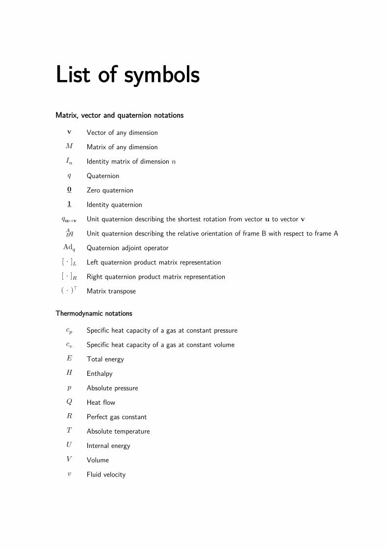
List of symbols

Matrix, vector and quaternion notations

𝐯 Vector of any dimension

𝑀 Matrix of any dimension

𝐼𝑛 Identity matrix of dimension 𝑛

𝑞 Quaternion

𝟎 Zero quaternion

𝟏 Identity quaternion

𝑞𝐮↦𝐯 Unit quaternion describing the shortest rotation from vector 𝐮 to vector 𝐯

𝑞𝐵𝐴 Unit quaternion describing the relative orientation of frame B with respect to frame A

Ad𝑞 Quaternion adjoint operator

[ ⋅ ]𝐿 Left quaternion product matrix representation

[ ⋅ ]𝑅 Right quaternion product matrix representation

( ⋅ )⊺ Matrix transpose

Thermodynamic notations

𝑐𝑝 Specific heat capacity of a gas at constant pressure

𝑐𝑣 Specific heat capacity of a gas at constant volume

𝐸 Total energy

𝐻 Enthalpy

𝑝 Absolute pressure

𝑄 Heat flow

𝑅 Perfect gas constant

𝑇 Absolute temperature

𝑈 Internal energy

𝑉 Volume

𝑣 Fluid velocity

xii List of symbols

𝛾 Heat capacity ratio

𝜆 Friction coefficient

𝜇 Fluid dynamic viscosity

𝜌 Fluid density

Other notations

𝑥 ̇ First time derivative of variable 𝑥

List of acronyms

AHRS Attitude and Heading Reference System

AIA Articulated Inspection Arm

CAD Computer Aided Design

CEA The French Alternative Energies and Atomic Energy Commission

FBG Fiber Bragg Gratings

FEA Finite Elements Analysis

FFA Flexible Fluidic Actuator

FOIM Fiber Optic Intensity Modulation

HMI Human Machine Interaction

IMU Inertial Measurement Unit

MARG Magnetic Angular Rate Gravity sensor

MEMS Micro-electromechanical Systems

MRI Magnetic Resonance Imaging

PAC Articulated Carrier for Cell Inspection

PWM Pulse Width Modulation

RMSE Root Mean Square Error

SMA Shape Memory Alloy

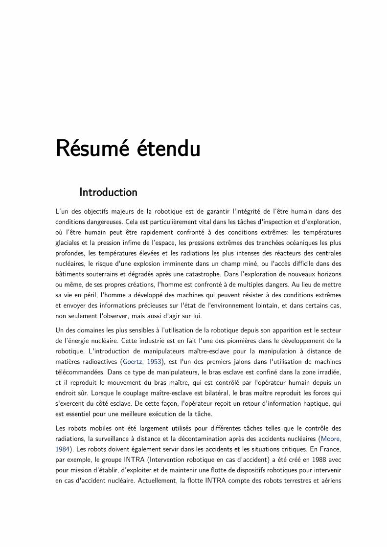
Résumé étendu

Introduction

L’un des objectifs majeurs de la robotique est de garantir l'intégrité de l’être humain dans des

conditions dangereuses. Cela est particulièrement vital dans les tâches d'inspection et d'exploration,

où l’être humain peut être rapidement confronté à des conditions extrêmes: les températures

glaciales et la pression infime de l’espace, les pressions extrêmes des tranchées océaniques les plus

profondes, les températures élevées et les radiations les plus intenses des réacteurs des centrales

nucléaires, le risque d'une explosion imminente dans un champ miné, ou l'accès difficile dans des

bâtiments souterrains et dégradés après une catastrophe. Dans l'exploration de nouveaux horizons

ou même, de ses propres créations, l'homme est confronté à de multiples dangers. Au lieu de mettre

sa vie en péril, l'homme a développé des machines qui peuvent résister à des conditions extrêmes

et envoyer des informations précieuses sur l'état de l'environnement lointain, et dans certains cas,

non seulement l'observer, mais aussi d'agir sur lui.

Un des domaines les plus sensibles à l’utilisation de la robotique depuis son apparition est le secteur

de l’énergie nucléaire. Cette industrie est en fait l'une des pionnières dans le développement de la

robotique. L'introduction de manipulateurs maître-esclave pour la manipulation à distance de

matières radioactives (Goertz, 1953), est l'un des premiers jalons dans l'utilisation de machines

télécommandées. Dans ce type de manipulateurs, le bras esclave est confiné dans la zone irradiée,

et il reproduit le mouvement du bras maître, qui est contrôlé par l'opérateur humain depuis un

endroit sûr. Lorsque le couplage maître-esclave est bilatéral, le bras maître reproduit les forces qui

s'exercent du côté esclave. De cette façon, l'opérateur reçoit un retour d'information haptique, qui

est essentiel pour une meilleure exécution de la tâche.

Les robots mobiles ont été largement utilisés pour différentes tâches telles que le contrôle des

radiations, la surveillance à distance et la décontamination après des accidents nucléaires (Moore,

1984). Les robots doivent également servir dans les accidents et les situations critiques. En France,

par exemple, le groupe INTRA (Intervention robotique en cas d'accident) a été créé en 1988 avec

pour mission d'établir, d'exploiter et de maintenir une flotte de dispositifs robotiques pour intervenir

en cas d'accident nucléaire. Actuellement, la flotte INTRA compte des robots terrestres et aériens

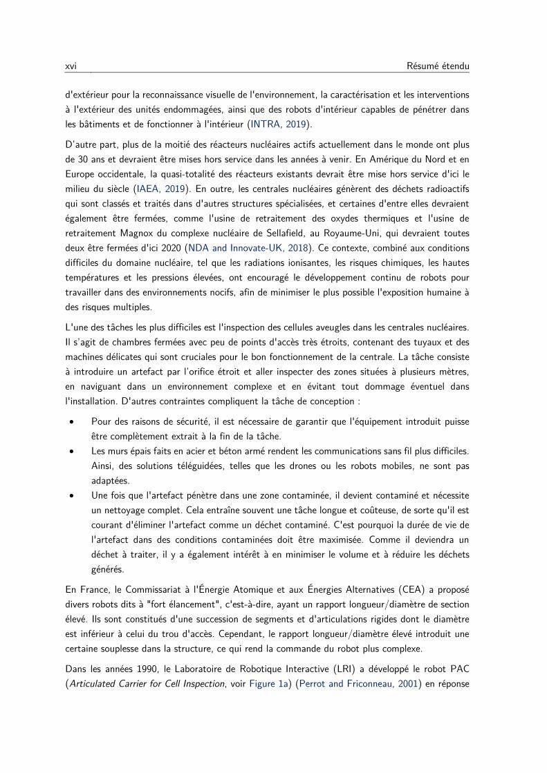
xvi Résumé étendu

d'extérieur pour la reconnaissance visuelle de l'environnement, la caractérisation et les interventions

à l'extérieur des unités endommagées, ainsi que des robots d'intérieur capables de pénétrer dans

les bâtiments et de fonctionner à l'intérieur (INTRA, 2019).

D’autre part, plus de la moitié des réacteurs nucléaires actifs actuellement dans le monde ont plus

de 30 ans et devraient être mises hors service dans les années à venir. En Amérique du Nord et en

Europe occidentale, la quasi-totalité des réacteurs existants devrait être mise hors service d'ici le

milieu du siècle (IAEA, 2019). En outre, les centrales nucléaires génèrent des déchets radioactifs

qui sont classés et traités dans d'autres structures spécialisées, et certaines d'entre elles devraient

également être fermées, comme l'usine de retraitement des oxydes thermiques et l'usine de

retraitement Magnox du complexe nucléaire de Sellafield, au Royaume-Uni, qui devraient toutes

deux être fermées d'ici 2020 (NDA and Innovate-UK, 2018). Ce contexte, combiné aux conditions

difficiles du domaine nucléaire, tel que les radiations ionisantes, les risques chimiques, les hautes

températures et les pressions élevées, ont encouragé le développement continu de robots pour

travailler dans des environnements nocifs, afin de minimiser le plus possible l'exposition humaine à

des risques multiples.

L'une des tâches les plus difficiles est l'inspection des cellules aveugles dans les centrales nucléaires.

Il s’agit de chambres fermées avec peu de points d'accès très étroits, contenant des tuyaux et des

machines délicates qui sont cruciales pour le bon fonctionnement de la centrale. La tâche consiste

à introduire un artefact par l’orifice étroit et aller inspecter des zones situées à plusieurs mètres,

en naviguant dans un environnement complexe et en évitant tout dommage éventuel dans

l'installation. D'autres contraintes compliquent la tâche de conception :

• Pour des raisons de sécurité, il est nécessaire de garantir que l'équipement introduit puisse

être complètement extrait à la fin de la tâche.

• Les murs épais faits en acier et béton armé rendent les communications sans fil plus difficiles.

Ainsi, des solutions téléguidées, telles que les drones ou les robots mobiles, ne sont pas

adaptées.

• Une fois que l'artefact pénètre dans une zone contaminée, il devient contaminé et nécessite

un nettoyage complet. Cela entraîne souvent une tâche longue et coûteuse, de sorte qu'il est

courant d'éliminer l'artefact comme un déchet contaminé. C'est pourquoi la durée de vie de

l'artefact dans des conditions contaminées doit être maximisée. Comme il deviendra un

déchet à traiter, il y a également intérêt à en minimiser le volume et à réduire les déchets

générés.

En France, le Commissariat à l'Énergie Atomique et aux Énergies Alternatives (CEA) a proposé

divers robots dits à "fort élancement", c'est-à-dire, ayant un rapport longueur/diamètre de section

élevé. Ils sont constitués d'une succession de segments et d'articulations rigides dont le diamètre

est inférieur à celui du trou d'accès. Cependant, le rapport longueur/diamètre élevé introduit une

certaine souplesse dans la structure, ce qui rend la commande du robot plus complexe.

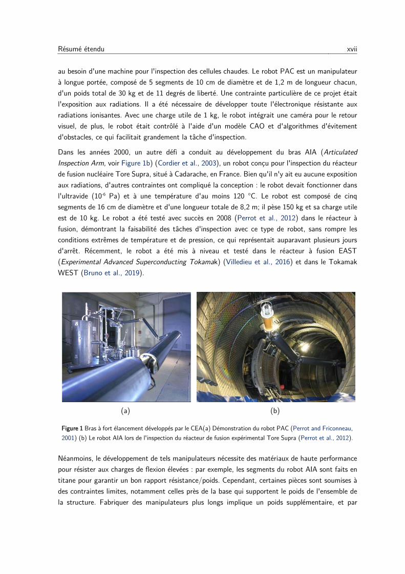
Dans les années 1990, le Laboratoire de Robotique Interactive (LRI) a développé le robot PAC

(Articulated Carrier for Cell Inspection, voir Figure 1a) (Perrot and Friconneau, 2001) en réponse

Résumé étendu xvii

au besoin d'une machine pour l'inspection des cellules chaudes. Le robot PAC est un manipulateur

à longue portée, composé de 5 segments de 10 cm de diamètre et de 1,2 m de longueur chacun,

d'un poids total de 30 kg et de 11 degrés de liberté. Une contrainte particulière de ce projet était

l'exposition aux radiations. Il a été nécessaire de développer toute l'électronique résistante aux

radiations ionisantes. Avec une charge utile de 1 kg, le robot intégrait une caméra pour le retour

visuel, de plus, le robot était contrôlé à l'aide d'un modèle CAO et d'algorithmes d'évitement

d'obstacles, ce qui facilitait grandement la tâche d'inspection.

Dans les années 2000, un autre défi a conduit au développement du bras AIA (Articulated

Inspection Arm, voir Figure 1b) (Cordier et al., 2003), un robot conçu pour l'inspection du réacteur

de fusion nucléaire Tore Supra, situé à Cadarache, en France. Bien qu'il n'y ait eu aucune exposition

aux radiations, d'autres contraintes ont compliqué la conception : le robot devait fonctionner dans

l'ultravide (10-6 Pa) et à une température d'au moins 120 °C. Le robot est composé de cinq

segments de 16 cm de diamètre et d'une longueur totale de 8,2 m; il pèse 150 kg et sa charge utile

est de 10 kg. Le robot a été testé avec succès en 2008 (Perrot et al., 2012) dans le réacteur à

fusion, démontrant la faisabilité des tâches d'inspection avec ce type de robot, sans rompre les

conditions extrêmes de température et de pression, ce qui représentait auparavant plusieurs jours

d'arrêt. Récemment, le robot a été mis à niveau et testé dans le réacteur à fusion EAST

(Experimental Advanced Superconducting Tokamak) (Villedieu et al., 2016) et dans le Tokamak

WEST (Bruno et al., 2019).

(a) (b)

Figure 1 Bras à fort élancement développés par le CEA(a) Démonstration du robot PAC (Perrot and Friconneau,

2001) (b) Le robot AIA lors de l'inspection du réacteur de fusion expérimental Tore Supra (Perrot et al., 2012).

Néanmoins, le développement de tels manipulateurs nécessite des matériaux de haute performance

pour résister aux charges de flexion élevées : par exemple, les segments du robot AIA sont faits en

titane pour garantir un bon rapport résistance/poids. Cependant, certaines pièces sont soumises à

des contraintes limites, notamment celles près de la base qui supportent le poids de l'ensemble de

la structure. Fabriquer des manipulateurs plus longs implique un poids supplémentaire, et par

xviii Résumé étendu

conséquent, des matériaux qui résistent aux charges dérivées, en gardant à l'esprit que le diamètre

du segment doit rester inchangé pour entrer par le même orifice d'accès. L'optimisation des

propriétés des matériaux a été poussée à ses limites, et la marge d'amélioration est très faible en

rapport à l’investissement nécessaire.

Les robots gonflables, une rupture technologique

Le principal problème dans la conception de manipulateurs plus longs est le poids. Pour contourner

cette barrière, le Service de Robotique Interactive du CEA travaille depuis 2011 sur un nouveau

concept de manipulateur : un bras ultraléger gonflable (Voisembert et al., 2011). Il est constitué

d'une chambre à air cylindrique, articulée en différents points, donnant lieu à une succession de

segments et de liaisons de type rotule. Constitué d'une membrane fine très résistante, il est léger,

et la pression interne lui confère une rigidité suffisante pour supporter son poids.

Avantages

Un robot avec une structure gonflable présente plusieurs avantages :

• Des liens plus longs peuvent être obtenus avec un minimum de masse supplémentaire. Cela

signifie que des manipulateurs plus longs peuvent être obtenus pour avoir un volume de

travail plus important.

• Les coûts de fabrication peuvent être réduits de manière impressionnante, car les matériaux

utilisés sont moins spécialisés et moins chers.

• La compressibilité de l'air confère de la souplesse à l'ensemble de la structure. C'est une

caractéristique vitale dans un manipulateur destiné à effectuer des tâches d'inspection dans

des environnements délicats, car il peut entrer en collision ou s'appuyer sur l'environnement

sans risque de l’endommager.

• Une structure gonflable a un volume réduit lorsqu'elle n'est pas gonflée. Cette propriété

est particulièrement avantageuse pour le transport, car la structure peut être emballée dans

un volume réduit et déployée rapidement pour une intervention. Mais elle est également

avantageuse pour son élimination : lorsqu'il travaille dans une zone contaminée, le robot

finit lui aussi par être contaminé, et il peut finir comme un déchet supplémentaire. Son

volume réduit garantit qu'il représentera une part minimale des déchets générés.

Le coût réduit ainsi que la facilité de transport et de déploiement pourraient élargir le champ

d’applications. Le transfert technologique du cas particulier du domaine nucléaire vers d'autres

secteurs pourrait devenir possible.

La faisabilité de ce type de manipulateurs a été démontrée par (Voisembert, 2012) et renforcée par

de multiples brevets (Riwan and Voisembert, 2011; Voisembert, 2015; Voisembert, 2018). Le

développement continu de ces travaux a permis un partenariat entre le CEA et Warein, une

entreprise française spécialisée dans la fabrication de tissus techniques. Fruit de cette collaboration,

Résumé étendu xix

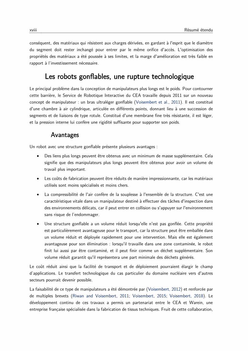
la faisabilité d’un prototype dont la structure et les actionneurs sont faits en tissu a pu être validée

(voir Figure 2). La longueur totale de la structure ainsi que le nombre de segments et d’articulations

sont adaptables selon le besoin, et le tout peut être emballé dans un sac à dos pour faciliter le

transport.

(a) (b)

Figure 2 Démonstration du bras ultraléger gonflable (a) Démonstration du bras ultraléger gonflable dans

l’inspection du fuselage d’un avion (b) Inspection en environnement industriel.

Même si les matériaux employés ne sont pas encore conformes aux exigences nucléaires,

l’application d’un tel robot dans d'autres domaines a prouvé son efficacité. En 2015, un prototype

a été utilisé pour inspecter le fuselage d'un avion (DGA, 2015), démontrant son utilité dans

l'inspection de grandes surfaces. Son application pourrait se rependre dans d'autres secteurs où la

mobilité et l'agilité sont des facteurs clés, comme l'inspection d'objets suspects et le déminage, le

diagnostic d’ouvrages civils, ou même dans d'autres domaines où des structures gonflables sont

actuellement utilisées, comme les structures nomades pour les événements, le camping et les

divertissements.

Défis actuels

Malgré les nombreux avantages annoncés dans la dernière section, certains aspects ont entravé la

massification des robots ultralégers :

• La contrainte absolue de légèreté impose des choix sur les composants et la disposition du

système. Le mode de fonctionnement a totalement évolué par rapport à celui présenté dans

(Voisembert et al., 2011). Actuellement, chaque articulation est actionnée par deux

actionneurs pneumatiques textiles (décrits dans le chapitre 3), inventés et brevetés par

Warein. Ces actionneurs garantissent un rapport force/poids très important, mais étant

donné qu’ils n'ont pas encore été largement utilisés, leur comportement n'a jamais été

caractérisé.

• D'autre part, la commande du robot demeure une architecture en boucle ouverte. Cela

signifie que l'opérateur doit contrôler le gonflage et le dégonflage de chaque actionneur

xx Résumé étendu

pour entraîner une rotation dans chaque articulation. Il en résulte une tâche fastidieuse et

difficile, car l'opérateur doit avoir en permanence une vue directe sur l'ensemble du robot,

ce qui n’est pas garanti lors de l'inspection d'environnements confinés. L'absence d’une

commande en boucle fermée est principalement liée à l'absence d'un capteur de position,

qui est un élément crucial pour avoir le retour de l'état actuel du robot et appliquer les

corrections nécessaires pour atteindre la configuration désirée. En outre, les capteurs

classiques utilisés dans les robots rigides ne sont adaptés ni aux surfaces souples et

déformables ni aux articulations qui ne présentent pas d'axes de rotation bien définis.

Un autre obstacle au développement de la commande en boucle fermée est la nature du système

d'entraînement : la dynamique des systèmes pneumatiques est plus lente que celle de leurs

homologues électriques. De plus, le pneumatique présente un comportement fortement non linéaire.

Ces deux faits complexifient la synthèse d'un contrôleur, mais d'autres choix y contribuent

également :

• Pour contrôler le gonflage et le dégonflage de chaque actionneur, il a été décidé d'installer

un système d'électrovannes au lieu de servovalves. Ce choix a été basé sur deux critères :

le coût et le poids. Les électrovannes ont un mécanisme plus simple que les servovalves.

Elles sont donc plus légères et ne nécessitent pas de composants aussi coûteux que ceux

utilisés dans les servovalves. Alors qu'une servovalve coûte entre une centaine et un millier

de dollars et pèse quelques centaines de grammes, une électrovalve 2/2 voies peut coûter

quelques dizaines de dollars et peser quelques dizaines de grammes. Cependant, la nature

divergente de l'entrée (ouverte ou fermée) rend les lois de contrôle continu traditionnelles

inutiles, et des problèmes tels que la commutation à haute fréquence (chattering) peuvent

apparaître, réduisant considérablement la durée de vie de la vanne.

• L'emplacement des vannes et des capteurs pose une autre difficulté : Afin de maintenir la

structure aussi légère que possible, les vannes et les capteurs de pression sont situés à la

base du robot. Un tuyau assure la connexion entre chaque actionneur de la structure et la

vanne et le capteur de pression correspondants à la base du robot. La longueur de ces

tuyaux n'est pas négligeable. Par exemple, si le robot a une longueur totale de 6 m, des

tuyaux de 5 m de long seront nécessaires pour alimenter les actionneurs sur le dernier

maillon. L'actionnement et les mesures non colocalisées introduisent des pertes et des

retards ; il faut y remédier avec soin pour garantir la stabilité du contrôleur.

• Enfin, la souplesse inhérente à la structure gonflable doit être prise en compte afin de

contrôler la position de l'effecteur final le plus précisément possible, et d'atténuer les effets

des déformations et d’éventuelles vibrations.

Contributions

Le domaine de la robotique gonflable est vaste, car il reformule les bases de la robotique

conventionnelle sous tous ses aspects, en allant de l'actionnement et de la détection à la

Résumé étendu xxi

modélisation, l'identification et le contrôle. Ce travail de thèse vise à complémenter le travail déjà

effectué sur le bras gonflable. Ainsi, plusieurs développements théoriques et technologiques sont

proposés pour la mise en service opérationnelle du robot. Trois points que nous considérons comme

fondamentaux pour poursuivre le développement de la robotique gonflable et qui participeront à

réduire l'écart entre la recherche en laboratoire et sa mise en œuvre et son fonctionnement réels

sont abordés :

• La modélisation et la caractérisation d'un nouveau type d'actionneur pour les robots

gonflables qui respectent la contrainte de légèreté, mais qui, en même temps, peuvent

délivrer des forces importantes et effectuer le mouvement important.

• La proposition d'une approche de mesure basée sur l'utilisation d'un réseau de capteurs

MARG (Magnetic, Angle Rate, and Gravity). La solution répond aux contraintes des robots

gonflables, à savoir : elle n'affecte pas la conformité naturelle de la structure où elle est

intégrée. Enfin, elle est légère et peu coûteuse.

• La validation de schémas de commande adaptés au contrôle en position des articulations

du robot.

Organisation du manuscrit

L'organisation de ce travail de thèse est décrite ci-après :

Le chapitre 2 présente un état de l'art des structures gonflables, leurs avantages et leurs applications

actuelles. Il examine les développements en cours dans le domaine de la robotique souple, ses

avancées et les défis actuels. Enfin, il détaille la structure du robot gonflable étudié dans ces travaux

et compare ses caractéristiques avec d'autres robots trouvés dans la littérature.

Le chapitre 3 commence par l'état de l'art des actionneurs pneumatiques. Ensuite, il décrit les

actionneurs qui sont employés dans chaque articulation du robot. Tout d'abord, un prototype de

forme cylindrique est présenté, détaillant son principe de fonctionnement, une étude simplifiée de

sa cinématique et de la génération de force, ainsi que la caractérisation expérimentale. Ensuite, un

problème d'instabilité de ce concept est introduit et motive l'étude d'un autre concept de forme

conique. Comme dans le premier cas, une étude géométrique et une statique sont réalisées et

comparées aux résultats expérimentaux. Puis, la mise en œuvre d'une analyse par éléments finis

est présentée ainsi que les résultats de simulation obtenus.

Le chapitre 4 présente un état de l'art des capteurs de position qui ont été proposés dans d'autres

domaines et qui peuvent être utiles dans le contexte de la robotique souple et gonflable. Ensuite,

le problème de la mesure de la position articulaire entre deux corps est abordé à travers deux

approches : La première consiste à estimer l'angle entre deux corps à l'aide d'un magnétomètre à

trois axes fixé dans l'un des corps et perturbé par un aimant permanent fixé dans l'autre. Cette

approche n'a pas donné de bons résultats, ce qui a motivé l'exploration d'une deuxième approche,

exploitant les mesures de capteurs supplémentaires, à savoir les accéléromètres et les gyroscopes.

Cette méthode est basée sur l'estimation de l'orientation relative entre deux corps en utilisant des

xxii Résumé étendu

mesures vectorielles correspondantes dans des référentiels différents. Le contexte mathématique

des représentations des rotations dans l'espace est décrit, en accordant une importance particulière

à la représentation par quaternions. Cela servira de base à l'introduction d'un algorithme pour

l'estimation de l'orientation relative entre deux corps dans l'espace.

Le chapitre 5 présente le modèle dynamique du système d'actionnement, une approche du contrôle

de la position d'une articulation gonflable par le biais d'un contrôleur de mode d'élingage.

Enfin, le chapitre 6 présente les conclusions générales de ce travail de recherche et indique quelques

orientations et suggestions pour aborder d'éventuels travaux futurs.

Actionneur

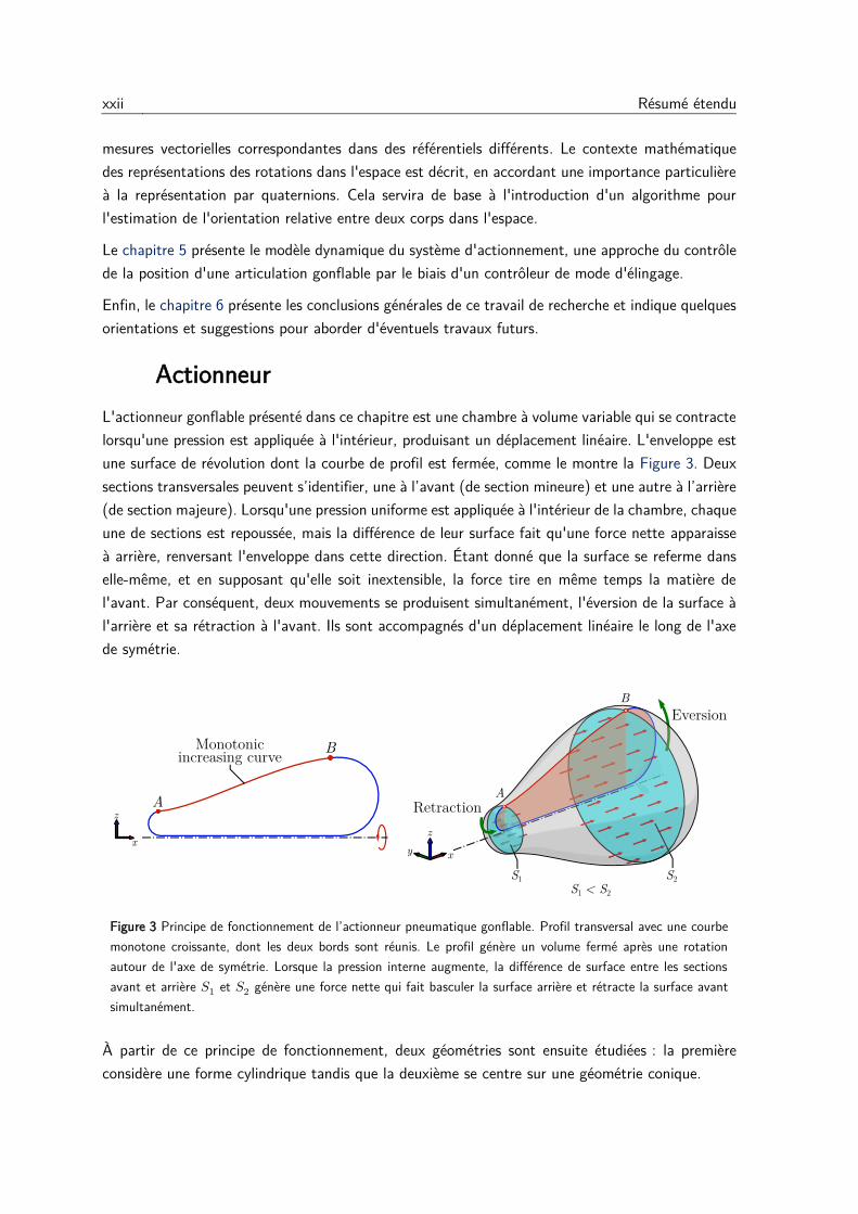
L'actionneur gonflable présenté dans ce chapitre est une chambre à volume variable qui se contracte

lorsqu'une pression est appliquée à l'intérieur, produisant un déplacement linéaire. L'enveloppe est

une surface de révolution dont la courbe de profil est fermée, comme le montre la Figure 3. Deux

sections transversales peuvent s’identifier, une à l’avant (de section mineure) et une autre à l’arrière

(de section majeure). Lorsqu'une pression uniforme est appliquée à l'intérieur de la chambre, chaque

une de sections est repoussée, mais la différence de leur surface fait qu'une force nette apparaisse

à arrière, renversant l'enveloppe dans cette direction. Étant donné que la surface se referme dans

elle-même, et en supposant qu'elle soit inextensible, la force tire en même temps la matière de

l'avant. Par conséquent, deux mouvements se produisent simultanément, l'éversion de la surface à

l'arrière et sa rétraction à l'avant. Ils sont accompagnés d'un déplacement linéaire le long de l'axe

de symétrie.

Figure 3 Principe de fonctionnement de l’actionneur pneumatique gonflable. Profil transversal avec une courbe

monotone croissante, dont les deux bords sont réunis. Le profil génère un volume fermé après une rotation

autour de l'axe de symétrie. Lorsque la pression interne augmente, la différence de surface entre les sections

avant et arrière 𝑆1 et 𝑆2 génère une force nette qui fait basculer la surface arrière et rétracte la surface avant

simultanément.

À partir de ce principe de fonctionnement, deux géométries sont ensuite étudiées : la première

considère une forme cylindrique tandis que la deuxième se centre sur une géométrie conique.

Résumé étendu xxiii

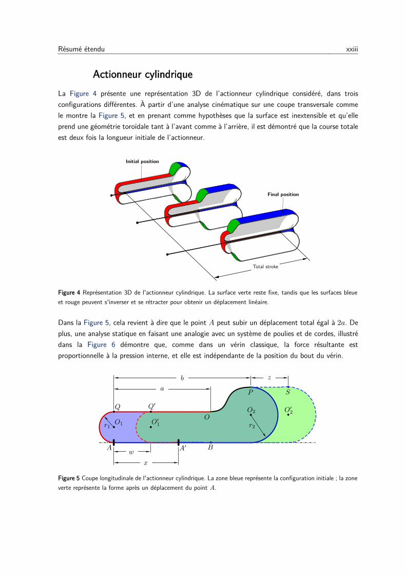
Actionneur cylindrique

La Figure 4 présente une représentation 3D de l’actionneur cylindrique considéré, dans trois

configurations différentes. À partir d’une analyse cinématique sur une coupe transversale comme

le montre la Figure 5, et en prenant comme hypothèses que la surface est inextensible et qu’elle

prend une géométrie toroïdale tant à l’avant comme à l’arrière, il est démontré que la course totale

est deux fois la longueur initiale de l’actionneur.

Figure 4 Représentation 3D de l'actionneur cylindrique. La surface verte reste fixe, tandis que les surfaces bleue

et rouge peuvent s'inverser et se rétracter pour obtenir un déplacement linéaire.

Dans la Figure 5, cela revient à dire que le point 𝐴 peut subir un déplacement total égal à 2𝑎. De

plus, une analyse statique en faisant une analogie avec un système de poulies et de cordes, illustré

dans la Figure 6 démontre que, comme dans un vérin classique, la force résultante est

proportionnelle à la pression interne, et elle est indépendante de la position du bout du vérin.

Figure 5 Coupe longitudinale de l'actionneur cylindrique. La zone bleue représente la configuration initiale ; la zone

verte représente la forme après un déplacement du point 𝐴.

xxiv Résumé étendu

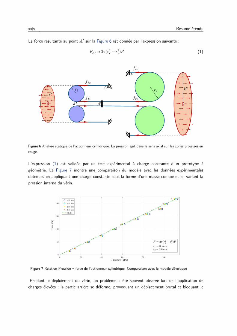
La force résultante au point 𝐴′ sur la Figure 6 est donnée par l’expression suivante :

𝐹𝐴′ ≈ 2𝜋(𝑟22 − 𝑟1

2)𝑃 (1)

Figure 6 Analyse statique de l’actionneur cylindrique. La pression agit dans le sens axial sur les zones projetées en

rouge.

L’expression (1) est validée par un test expérimental à charge constante d’un prototype à

géométrie. La Figure 7 montre une comparaison du modèle avec les données expérimentales

obtenues en appliquant une charge constante sous la forme d’une masse connue et en variant la

pression interne du vérin.

Figure 7 Relation Pression – force de l’actionneur cylindrique. Comparaison avec le modèle développé

Pendant le déploiement du vérin, un problème a été souvent observé lors de l'application de

charges élevées : la partie arrière se déforme, provoquant un déplacement brutal et bloquant le

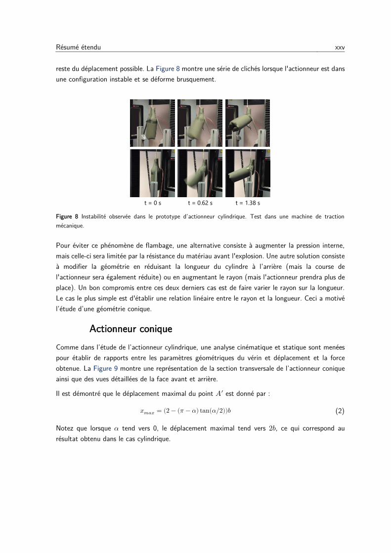
Résumé étendu xxv

reste du déplacement possible. La Figure 8 montre une série de clichés lorsque l'actionneur est dans

une configuration instable et se déforme brusquement.

Figure 8 Instabilité observée dans le prototype d’actionneur cylindrique. Test dans une machine de traction

mécanique.

Pour éviter ce phénomène de flambage, une alternative consiste à augmenter la pression interne,

mais celle-ci sera limitée par la résistance du matériau avant l'explosion. Une autre solution consiste

à modifier la géométrie en réduisant la longueur du cylindre à l’arrière (mais la course de

l'actionneur sera également réduite) ou en augmentant le rayon (mais l'actionneur prendra plus de

place). Un bon compromis entre ces deux derniers cas est de faire varier le rayon sur la longueur.

Le cas le plus simple est d'établir une relation linéaire entre le rayon et la longueur. Ceci a motivé

l’étude d’une géométrie conique.

Actionneur conique

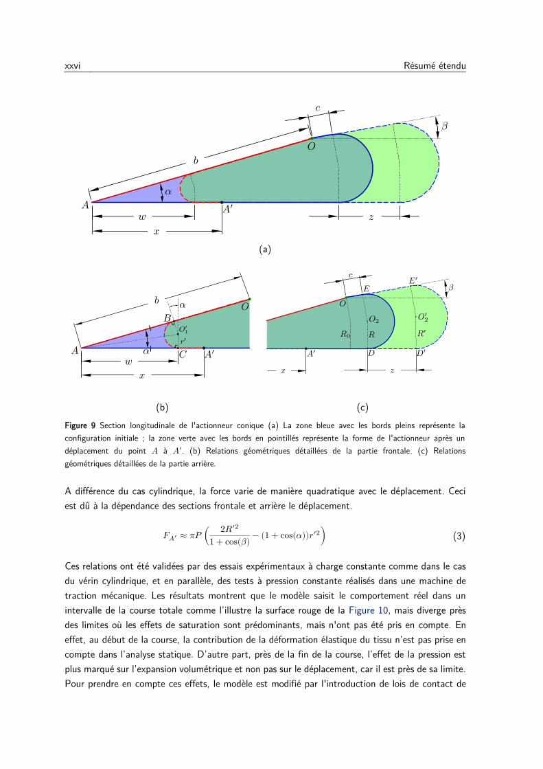
Comme dans l’étude de l’actionneur cylindrique, une analyse cinématique et statique sont menées

pour établir de rapports entre les paramètres géométriques du vérin et déplacement et la force

obtenue. La Figure 9 montre une représentation de la section transversale de l’actionneur conique

ainsi que des vues détaillées de la face avant et arrière.

Il est démontré que le déplacement maximal du point 𝐴′ est donné par :

𝑥𝑚𝑎𝑥 = (2 − (𝜋 − 𝛼) tan(𝛼 2⁄ ))𝑏 (2)

Notez que lorsque 𝛼 tend vers 0, le déplacement maximal tend vers 2𝑏, ce qui correspond au

résultat obtenu dans le cas cylindrique.

xxvi Résumé étendu

(a)

(b) (c)

Figure 9 Section longitudinale de l'actionneur conique (a) La zone bleue avec les bords pleins représente la

configuration initiale ; la zone verte avec les bords en pointillés représente la forme de l'actionneur après un

déplacement du point 𝐴 à 𝐴′. (b) Relations géométriques détaillées de la partie frontale. (c) Relations

géométriques détaillées de la partie arrière.

A différence du cas cylindrique, la force varie de manière quadratique avec le déplacement. Ceci

est dû à la dépendance des sections frontale et arrière le déplacement.

𝐹𝐴′ ≈ 𝜋𝑃 (2𝑅′2

1 + cos(𝛽)− (1 + cos(𝛼))𝑟′2) (3)

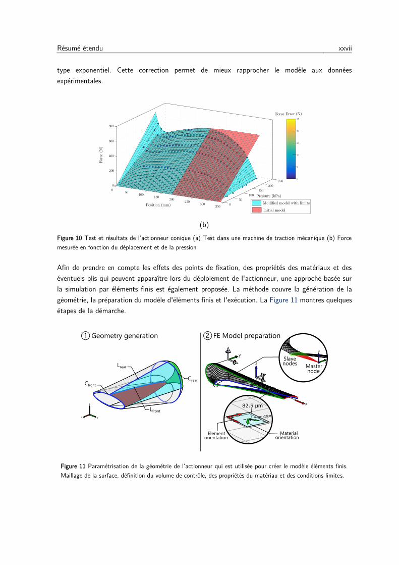
Ces relations ont été validées par des essais expérimentaux à charge constante comme dans le cas

du vérin cylindrique, et en parallèle, des tests à pression constante réalisés dans une machine de

traction mécanique. Les résultats montrent que le modèle saisit le comportement réel dans un

intervalle de la course totale comme l’illustre la surface rouge de la Figure 10, mais diverge près

des limites où les effets de saturation sont prédominants, mais n'ont pas été pris en compte. En

effet, au début de la course, la contribution de la déformation élastique du tissu n’est pas prise en

compte dans l’analyse statique. D’autre part, près de la fin de la course, l’effet de la pression est

plus marqué sur l’expansion volumétrique et non pas sur le déplacement, car il est près de sa limite.

Pour prendre en compte ces effets, le modèle est modifié par l'introduction de lois de contact de

Résumé étendu xxvii

type exponentiel. Cette correction permet de mieux rapprocher le modèle aux données

expérimentales.

(b)

Figure 10 Test et résultats de l’actionneur conique (a) Test dans une machine de traction mécanique (b) Force

mesurée en fonction du déplacement et de la pression

Afin de prendre en compte les effets des points de fixation, des propriétés des matériaux et des

éventuels plis qui peuvent apparaître lors du déploiement de l'actionneur, une approche basée sur

la simulation par éléments finis est également proposée. La méthode couvre la génération de la

géométrie, la préparation du modèle d'éléments finis et l'exécution. La Figure 11 montres quelques

étapes de la démarche.

Figure 11 Paramétrisation de la géométrie de l’actionneur qui est utilisée pour créer le modèle éléments finis.

Maillage de la surface, définition du volume de contrôle, des propriétés du matériau et des conditions limites.

xxviii Résumé étendu

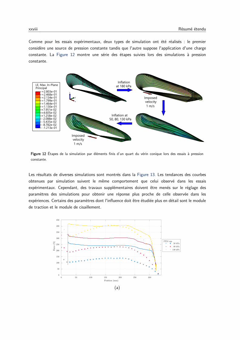
Comme pour les essais expérimentaux, deux types de simulation ont été réalisés : le premier

considère une source de pression constante tandis que l'autre suppose l'application d'une charge

constante. La Figure 12 montre une série des étapes suivies lors des simulations à pression

constante.

Figure 12 Étapes de la simulation par éléments finis d’un quart du vérin conique lors des essais à pression

constante.

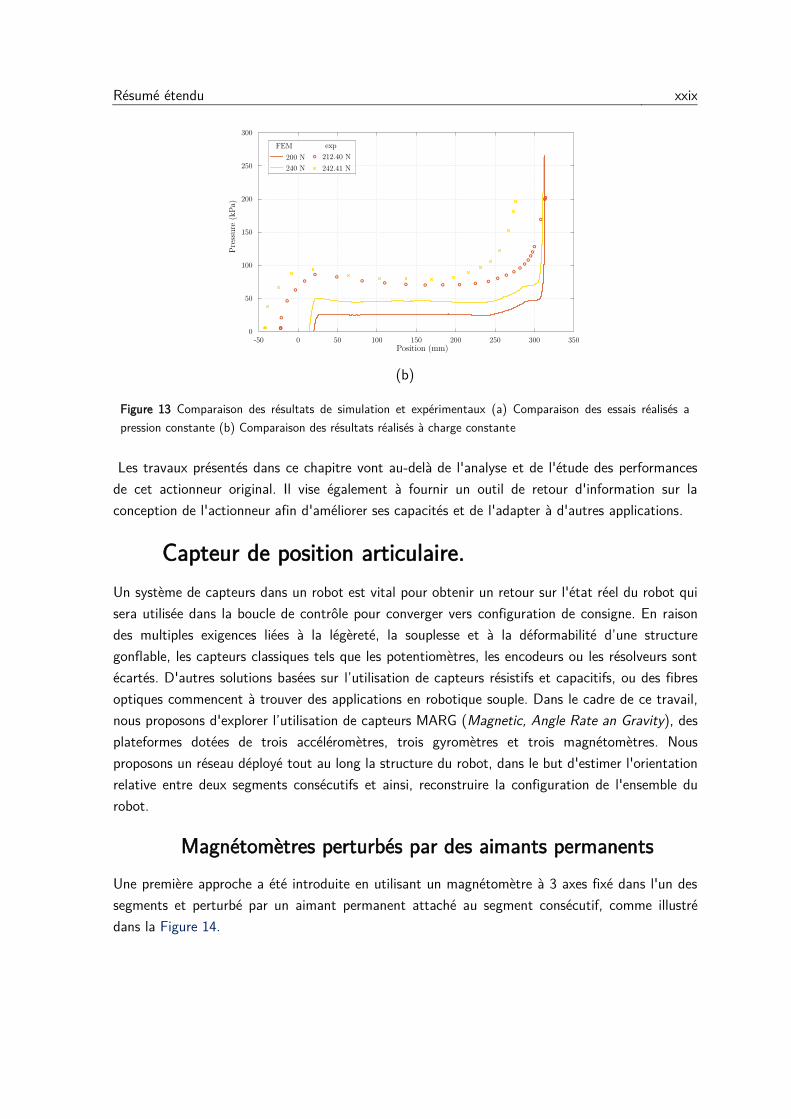
Les résultats de diverses simulations sont montrés dans la Figure 13. Les tendances des courbes

obtenues par simulation suivent le même comportement que celui observé dans les essais

expérimentaux. Cependant, des travaux supplémentaires doivent être menés sur le réglage des

paramètres des simulations pour obtenir une réponse plus proche de celle observée dans les

expériences. Certains des paramètres dont l'influence doit être étudiée plus en détail sont le module

de traction et le module de cisaillement.

(a)

Résumé étendu xxix

(b)

Figure 13 Comparaison des résultats de simulation et expérimentaux (a) Comparaison des essais réalisés a

pression constante (b) Comparaison des résultats réalisés à charge constante

Les travaux présentés dans ce chapitre vont au-delà de l'analyse et de l'étude des performances

de cet actionneur original. Il vise également à fournir un outil de retour d'information sur la

conception de l'actionneur afin d'améliorer ses capacités et de l'adapter à d'autres applications.

Capteur de position articulaire.

Un système de capteurs dans un robot est vital pour obtenir un retour sur l'état réel du robot qui

sera utilisée dans la boucle de contrôle pour converger vers configuration de consigne. En raison

des multiples exigences liées à la légèreté, la souplesse et à la déformabilité d’une structure

gonflable, les capteurs classiques tels que les potentiomètres, les encodeurs ou les résolveurs sont

écartés. D'autres solutions basées sur l’utilisation de capteurs résistifs et capacitifs, ou des fibres

optiques commencent à trouver des applications en robotique souple. Dans le cadre de ce travail,

nous proposons d'explorer l’utilisation de capteurs MARG (Magnetic, Angle Rate an Gravity), des

plateformes dotées de trois accéléromètres, trois gyromètres et trois magnétomètres. Nous

proposons un réseau déployé tout au long la structure du robot, dans le but d'estimer l'orientation

relative entre deux segments consécutifs et ainsi, reconstruire la configuration de l'ensemble du

robot.

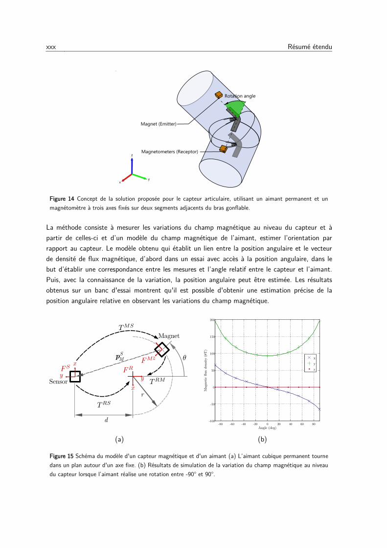
Magnétomètres perturbés par des aimants permanents

Une première approche a été introduite en utilisant un magnétomètre à 3 axes fixé dans l'un des

segments et perturbé par un aimant permanent attaché au segment consécutif, comme illustré

dans la Figure 14.

xxx Résumé étendu

Figure 14 Concept de la solution proposée pour le capteur articulaire, utilisant un aimant permanent et un

magnétomètre à trois axes fixés sur deux segments adjacents du bras gonflable.

La méthode consiste à mesurer les variations du champ magnétique au niveau du capteur et à

partir de celles-ci et d’un modèle du champ magnétique de l’aimant, estimer l’orientation par

rapport au capteur. Le modèle obtenu qui établit un lien entre la position angulaire et le vecteur

de densité de flux magnétique, d’abord dans un essai avec accès à la position angulaire, dans le

but d’établir une correspondance entre les mesures et l’angle relatif entre le capteur et l’aimant.

Puis, avec la connaissance de la variation, la position angulaire peut être estimée. Les résultats

obtenus sur un banc d'essai montrent qu'il est possible d'obtenir une estimation précise de la

position angulaire relative en observant les variations du champ magnétique.

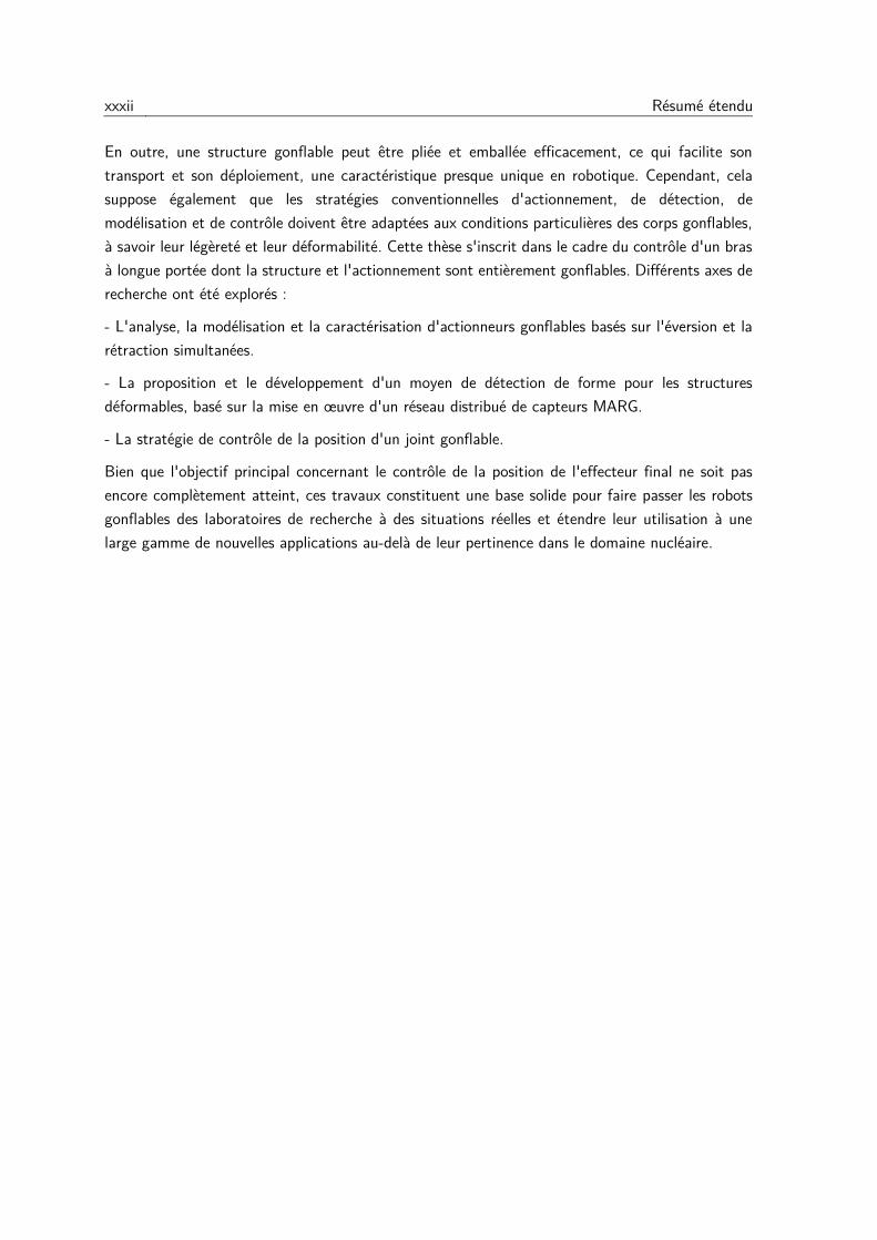
(a) (b)

Figure 15 Schéma du modèle d'un capteur magnétique et d'un aimant (a) L’aimant cubique permanent tourne

dans un plan autour d'un axe fixe. (b) Résultats de simulation de la variation du champ magnétique au niveau

du capteur lorsque l’aimant réalise une rotation entre -90° et 90°.

Résumé étendu xxxi

La mise en œuvre sur le robot gonflable a été plus difficile, car les supports sur lesquels le capteur

et l'aimant étaient fixés étaient déformés par l'actionnement des articulations, ce qui affectait la

répétabilité des mesures du capteur. Les travaux futurs pourraient être orientés dans deux

directions.

Afin de tirer pleinement profit de toutes les mesures disponibles dans chaque capteur MARG, une

approche d'orientation relative a été développée. Elle introduit une nouvelle solution fermée pour

l'estimation de l'orientation à partir de deux ensembles d'observations vectorielles, ce qui peut être

considéré comme une généralisation d'une méthode existante. L'amélioration repose sur

l'indépendance des vecteurs de référence choisis, il est donc possible d'estimer directement

l'orientation relative entre deux trames mobiles, au lieu de déterminer leur orientation absolue par

rapport à une trame fixe et de trouver ensuite la rotation relative. L'approche prend également en

compte l'estimation de l'orientation relative à partir des mesures du taux d'angle dans les deux

cadres mobiles. Enfin, les deux estimations sont fusionnées dans une structure de filtre

complémentaire, ce qui permet d'obtenir une estimation plus fiable. L'approche a été validée par

simulation, mais la mise en œuvre expérimentale est en attente et fera partie des travaux futurs.

Les développements ultérieurs pourraient être axés sur l'étalonnage du capteur en fonction de

l'orientation relative du corps. Notre travail s'est concentré sur l'estimation de l'orientation, mais

l'estimation de la position pourrait également être envisagée. Le principal problème de l'estimation

de la position à l'aide de capteurs inertiels est la dérive dans le temps, due à l'intégration de signaux

bruyants. Cependant, étant donné que les capteurs sont attachés aux maillons d'une chaîne série

au lieu d'êtres flottants, des contraintes cinématiques sont introduites et qui pourraient être

exploitées conjointement avec le modèle géométrique et cinématique du robot, pour obtenir une

estimation robuste aux effets dynamiques. Le principe de cette approche est décrit dans (Kok et

al., 2014 ; Laidig et al., 2017).

Bien que les deux méthodes proposées puissent paraître disjonctives, elles sont complémentaires.

L'utilisation d'un aimant permanent comme source de référence magnétique plus fiable pourrait

être intégrée dans l'estimation de l'orientation relative, car l'un de ses points forts est qu'aucune

connaissance préalable du champ de référence n'est nécessaire. Pour obtenir un champ magnétique

plus uniforme en utilisant des aimants permanents, il pourrait être intéressant d'expérimenter avec

d'autres arrangements d'aimants, par exemple, le réseau de Halbach (Halbach, 1981) qui augmente

le champ magnétique d'un côté du réseau tout en annulant le champ proche de zéro de l'autre

côté.

Conclusions

La robotique souple est un domaine en plein développement et en expansion. Bien que l'attention

se porte principalement vers les robots souples en élastomères, un autre domaine prometteur est

lié aux robots gonflables. Leur légèreté intrinsèque et leur souplesse en font des candidats appropriés

pour les applications où une interaction sûre avec l'environnement est capitale, comme la

collaboration homme-robot, la manipulation robotique ou l'inspection d'environnements dangereux.

xxxii Résumé étendu

En outre, une structure gonflable peut être pliée et emballée efficacement, ce qui facilite son

transport et son déploiement, une caractéristique presque unique en robotique. Cependant, cela

suppose également que les stratégies conventionnelles d'actionnement, de détection, de

modélisation et de contrôle doivent être adaptées aux conditions particulières des corps gonflables,

à savoir leur légèreté et leur déformabilité. Cette thèse s'inscrit dans le cadre du contrôle d'un bras

à longue portée dont la structure et l'actionnement sont entièrement gonflables. Différents axes de

recherche ont été explorés :

- L'analyse, la modélisation et la caractérisation d'actionneurs gonflables basés sur l'éversion et la

rétraction simultanées.

- La proposition et le développement d'un moyen de détection de forme pour les structures

déformables, basé sur la mise en œuvre d'un réseau distribué de capteurs MARG.

- La stratégie de contrôle de la position d'un joint gonflable.

Bien que l'objectif principal concernant le contrôle de la position de l'effecteur final ne soit pas

encore complètement atteint, ces travaux constituent une base solide pour faire passer les robots

gonflables des laboratoires de recherche à des situations réelles et étendre leur utilisation à une

large gamme de nouvelles applications au-delà de leur pertinence dans le domaine nucléaire.

Chapter 1

Introduction

Be practical as well as generous in your

ideals. Keep your eyes on the stars, but

remember to keep your feet on the ground

― Theodore Roosevelt

Contents

1.1 Robotics for exploration and inspection................................................................. 1

1.2 Robotics for nuclear applications .......................................................................... 4

1.3 Inflatable robots, a technological breakthrough ...................................................... 8

1.3.1 Advantages ................................................................................................... 8

1.3.2 Current challenges ........................................................................................ 9

1.4 Contributions ................................................................................................... 10

1.5 Outline ............................................................................................................ 11

1.1 Robotics for exploration and inspection

One of the goals of robotics since its early days has been to ensure human integrity under risky

conditions. This is particularly relevant in inspection and exploration tasks, where human access

may be required under extreme conditions. From the freezing temperatures and the vacuum of the

space, the extreme pressures of the deepest ocean trenches, the intense radiation and high

temperatures of nuclear energy plants, to the risk of an imminent explosion in a mined field, or the

difficult access in subterranean and post-disaster degraded buildings, human faces multiple dangers

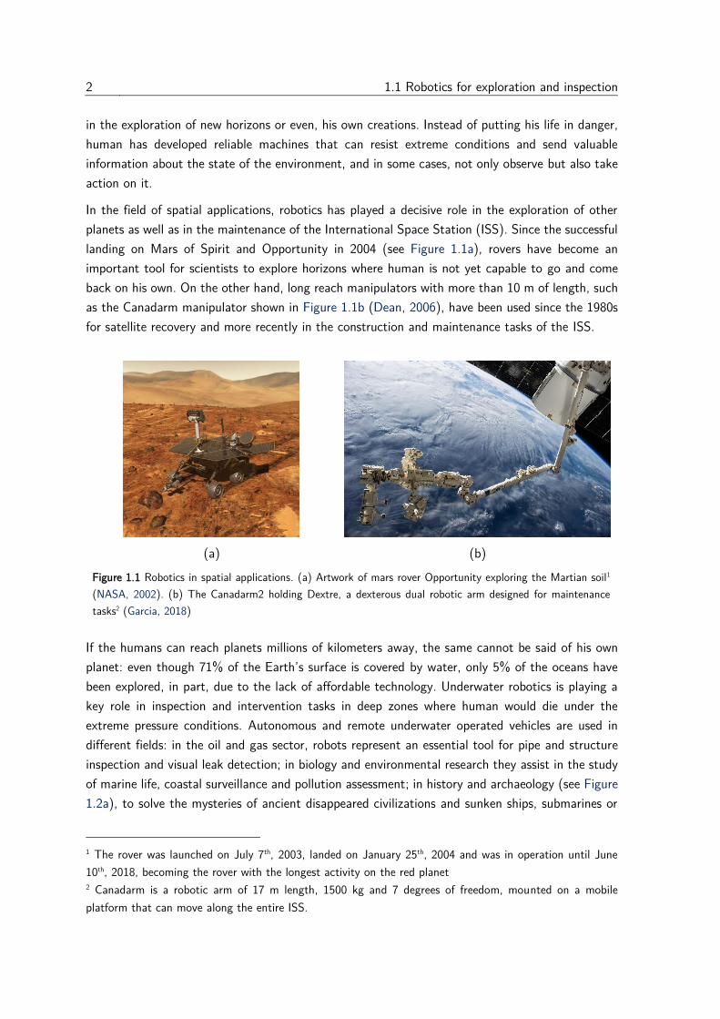
2 1.1 Robotics for exploration and inspection

in the exploration of new horizons or even, his own creations. Instead of putting his life in danger,

human has developed reliable machines that can resist extreme conditions and send valuable

information about the state of the environment, and in some cases, not only observe but also take

action on it.

In the field of spatial applications, robotics has played a decisive role in the exploration of other

planets as well as in the maintenance of the International Space Station (ISS). Since the successful

landing on Mars of Spirit and Opportunity in 2004 (see Figure 1.1a), rovers have become an

important tool for scientists to explore horizons where human is not yet capable to go and come

back on his own. On the other hand, long reach manipulators with more than 10 m of length, such

as the Canadarm manipulator shown in Figure 1.1b (Dean, 2006), have been used since the 1980s

for satellite recovery and more recently in the construction and maintenance tasks of the ISS.

(a) (b)

Figure 1.1 Robotics in spatial applications. (a) Artwork of mars rover Opportunity exploring the Martian soil1

(NASA, 2002). (b) The Canadarm2 holding Dextre, a dexterous dual robotic arm designed for maintenance

tasks2 (Garcia, 2018)

If the humans can reach planets millions of kilometers away, the same cannot be said of his own

planet: even though 71% of the Earth’s surface is covered by water, only 5% of the oceans have

been explored, in part, due to the lack of affordable technology. Underwater robotics is playing a

key role in inspection and intervention tasks in deep zones where human would die under the

extreme pressure conditions. Autonomous and remote underwater operated vehicles are used in

different fields: in the oil and gas sector, robots represent an essential tool for pipe and structure

inspection and visual leak detection; in biology and environmental research they assist in the study

of marine life, coastal surveillance and pollution assessment; in history and archaeology (see Figure

1.2a), to solve the mysteries of ancient disappeared civilizations and sunken ships, submarines or

1 The rover was launched on July 7th, 2003, landed on January 25th, 2004 and was in operation until June

10th, 2018, becoming the rover with the longest activity on the red planet 2 Canadarm is a robotic arm of 17 m length, 1500 kg and 7 degrees of freedom, mounted on a mobile

platform that can move along the entire ISS.

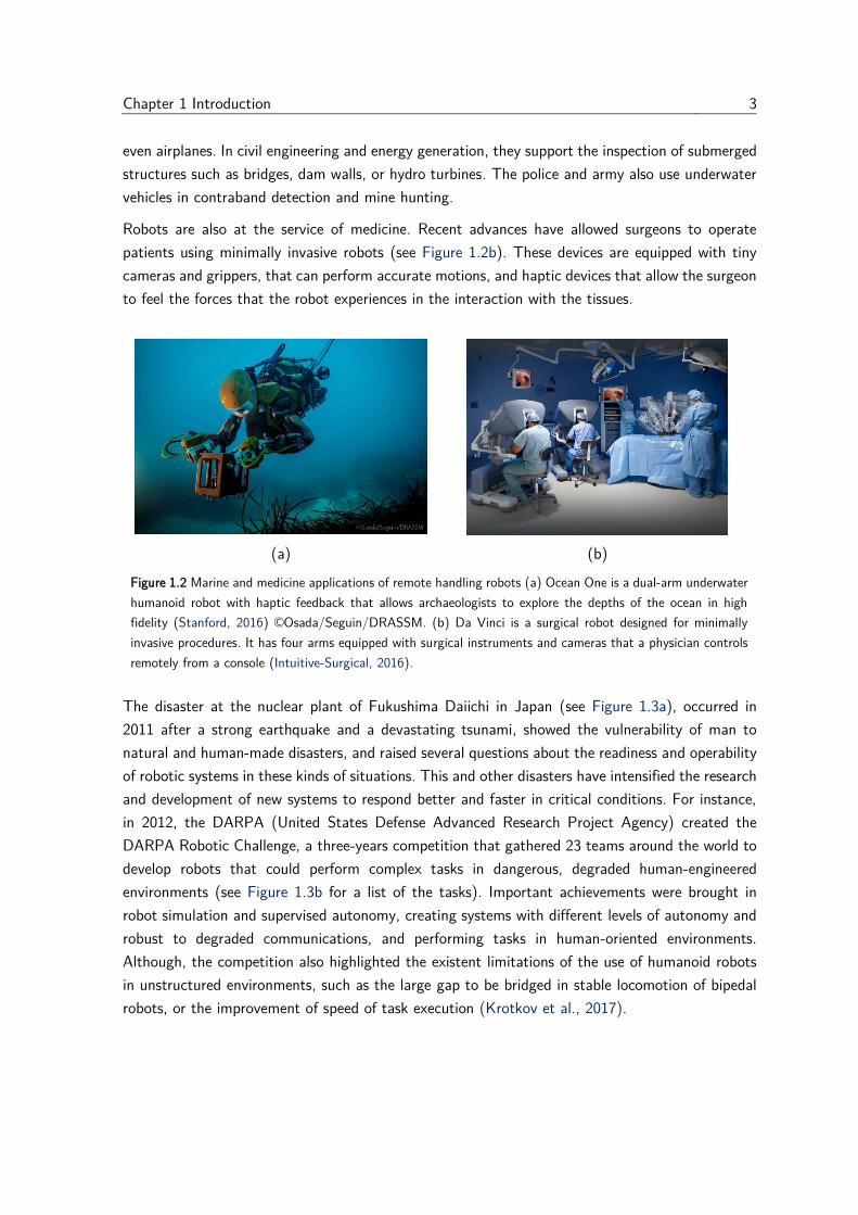
Chapter 1 Introduction 3

even airplanes. In civil engineering and energy generation, they support the inspection of submerged

structures such as bridges, dam walls, or hydro turbines. The police and army also use underwater

vehicles in contraband detection and mine hunting.

Robots are also at the service of medicine. Recent advances have allowed surgeons to operate

patients using minimally invasive robots (see Figure 1.2b). These devices are equipped with tiny

cameras and grippers, that can perform accurate motions, and haptic devices that allow the surgeon

to feel the forces that the robot experiences in the interaction with the tissues.

(a) (b)

Figure 1.2 Marine and medicine applications of remote handling robots (a) Ocean One is a dual-arm underwater

humanoid robot with haptic feedback that allows archaeologists to explore the depths of the ocean in high

fidelity (Stanford, 2016) ©Osada/Seguin/DRASSM. (b) Da Vinci is a surgical robot designed for minimally

invasive procedures. It has four arms equipped with surgical instruments and cameras that a physician controls

remotely from a console (Intuitive-Surgical, 2016).

The disaster at the nuclear plant of Fukushima Daiichi in Japan (see Figure 1.3a), occurred in

2011 after a strong earthquake and a devastating tsunami, showed the vulnerability of man to

natural and human-made disasters, and raised several questions about the readiness and operability

of robotic systems in these kinds of situations. This and other disasters have intensified the research

and development of new systems to respond better and faster in critical conditions. For instance,

in 2012, the DARPA (United States Defense Advanced Research Project Agency) created the

DARPA Robotic Challenge, a three-years competition that gathered 23 teams around the world to

develop robots that could perform complex tasks in dangerous, degraded human-engineered

environments (see Figure 1.3b for a list of the tasks). Important achievements were brought in

robot simulation and supervised autonomy, creating systems with different levels of autonomy and

robust to degraded communications, and performing tasks in human-oriented environments.

Although, the competition also highlighted the existent limitations of the use of humanoid robots

in unstructured environments, such as the large gap to be bridged in stable locomotion of bipedal

robots, or the improvement of speed of task execution (Krotkov et al., 2017).

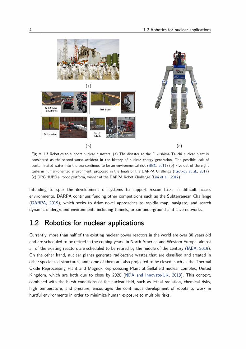
4 1.2 Robotics for nuclear applications

(a)

(b) (c)

Figure 1.3 Robotics to support nuclear disasters. (a) The disaster at the Fukushima Taiichi nuclear plant is

considered as the second-worst accident in the history of nuclear energy generation. The possible leak of

contaminated water into the sea continues to be an environmental risk (BBC, 2011) (b) Five out of the eight

tasks in human-oriented environment, proposed in the finals of the DARPA Challenge (Krotkov et al., 2017)

(c) DRC-HUBO+ robot platform, winner of the DARPA Robot Challenge (Lim et al., 2017)

Intending to spur the development of systems to support rescue tasks in difficult access

environments, DARPA continues funding other competitions such as the Subterranean Challenge

(DARPA, 2019), which seeks to drive novel approaches to rapidly map, navigate, and search

dynamic underground environments including tunnels, urban underground and cave networks.

1.2 Robotics for nuclear applications

Currently, more than half of the existing nuclear power reactors in the world are over 30 years old

and are scheduled to be retired in the coming years. In North America and Western Europe, almost

all of the existing reactors are scheduled to be retired by the middle of the century (IAEA, 2019).

On the other hand, nuclear plants generate radioactive wastes that are classified and treated in

other specialized structures, and some of them are also projected to be closed, such as the Thermal

Oxide Reprocessing Plant and Magnox Reprocessing Plant at Sellafield nuclear complex, United

Kingdom, which are both due to close by 2020 (NDA and Innovate-UK, 2018). This context,

combined with the harsh conditions of the nuclear field, such as lethal radiation, chemical risks,

high temperature, and pressure, encourages the continuous development of robots to work in

hurtful environments in order to minimize human exposure to multiple risks.

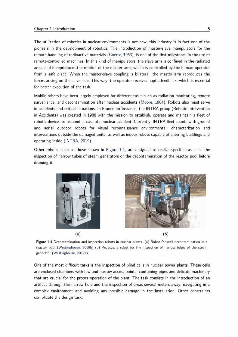
Chapter 1 Introduction 5

The utilization of robotics in nuclear environments is not new, this industry is in fact one of the

pioneers in the development of robotics. The introduction of master-slave manipulators for the

remote handling of radioactive materials (Goertz, 1953), is one of the first milestones in the use of

remote-controlled machines. In this kind of manipulators, the slave arm is confined in the radiated

area, and it reproduces the motion of the master arm, which is controlled by the human operator

from a safe place. When the master-slave coupling is bilateral, the master arm reproduces the

forces arising on the slave side. This way, the operator receives haptic feedback, which is essential

for better execution of the task.

Mobile robots have been largely employed for different tasks such as radiation monitoring, remote

surveillance, and decontamination after nuclear accidents (Moore, 1984). Robots also must serve

in accidents and critical situations. In France for instance, the INTRA group (Robotic Intervention

in Accidents) was created in 1988 with the mission to establish, operate and maintain a fleet of

robotic devices to respond in case of a nuclear accident. Currently, INTRA fleet counts with ground

and aerial outdoor robots for visual reconnaissance environmental, characterization and

interventions outside the damaged units, as well as indoor robots capable of entering buildings and

operating inside (INTRA, 2019).

Other robots, such as those shown in Figure 1.4, are designed to realize specific tasks, as the

inspection of narrow tubes of steam generators or the decontamination of the reactor pool before

draining it.

(a) (b)

Figure 1.4 Decontamination and inspection robots in nuclear plants. (a) Robot for wall decontamination in a

reactor pool (Westinghouse, 2019b) (b) Pegasys, a robot for the inspection of narrow tubes of the steam

generator (Westinghouse, 2019a)

One of the most difficult tasks is the inspection of blind cells in nuclear power plants. These cells

are enclosed chambers with few and narrow access points, containing pipes and delicate machinery

that are crucial for the proper operation of the plant. The task consists in the introduction of an

artifact through the narrow hole and the inspection of areas several meters away, navigating in a

complex environment and avoiding any possible damage in the installation. Other constraints

complicate the design task:

6 1.2 Robotics for nuclear applications

− For safety, it is required to guarantee that the introduced equipment can be completely

extracted at the end of the task.

− The thick steel re-enforced concrete walls complicate wireless communications. Thus,

solutions such as drones or untethered mobile robots are not suitable.

− Once the artifact enters in a contaminated area, it becomes contaminated and requires

a complete cleanup. It often results in an expensive and time-consuming task, so it is

common to dispose of the artifact as contaminated waste. For this reason, the artifact

lifespan in contaminated conditions must be maximized. As it will become a waste to

treat, there is also an interest to minimize its volume and reduce the generated waste.

This set of constraints and requirements has been addressed through different approaches:

OC Robotics is a British company that provides a robotic solution for the inspection of confined

and hazardous environments. It consists of a snake-like robot, composed of a series of connected

links and driven by wire ropes from the base of the robot. One of the models (OCRobotics, 2019)

is made of 12 links, and a total of 24 DDL. With a payload of 10 kg, it is possible to attach a wide

variety of tools to the end effector, such as a camera, a gripper or even a laser cutter. However,

the articulated length is limited to 3 m, which reduces the work volume.

Figure 1.5 Snake-like robot from OC Robotics , integrated with an inspection camera and lights tools

(OCRobotics, 2019)

In France, the Alternative and Atomic Energy Commission (CEA) has proposed various robots with

"high slenderness", i.e., having a high length to cross-section diameter ratio. They consist of a

succession of rigid segments and joints with a smaller diameter than the access hole. Equipped

with more than six orthogonal rotation axes, the kinematic redundancy allows avoiding obstacles

and inspecting every corner of the cell. However, the high length-to-diameter ratio introduces

flexibility in the structure, making the robot control more complex.

In the 1990s, the LRI (Interactive Robotics Laboratory) developed PAC (Articulated Carrier for

Cell Inspection, see Figure 1.6a) (Perrot and Friconneau, 2001) in response to an expressed need

of a machine for hot cell inspection. PAC is a long-range robot, consisting of 5 segments of 10 cm

diameter and 1.2 m length each, a total weight of 30 kg, and 11 degrees of freedom. A particular

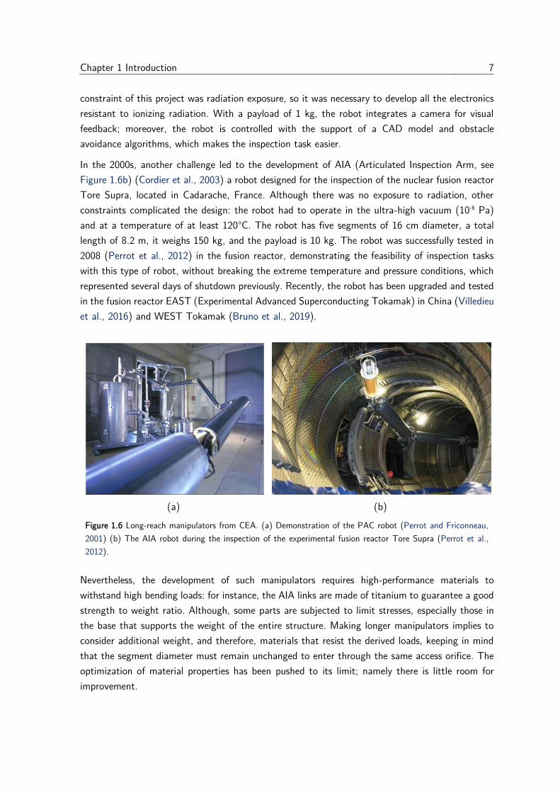
Chapter 1 Introduction 7

constraint of this project was radiation exposure, so it was necessary to develop all the electronics

resistant to ionizing radiation. With a payload of 1 kg, the robot integrates a camera for visual

feedback; moreover, the robot is controlled with the support of a CAD model and obstacle

avoidance algorithms, which makes the inspection task easier.

In the 2000s, another challenge led to the development of AIA (Articulated Inspection Arm, see

Figure 1.6b) (Cordier et al., 2003) a robot designed for the inspection of the nuclear fusion reactor

Tore Supra, located in Cadarache, France. Although there was no exposure to radiation, other

constraints complicated the design: the robot had to operate in the ultra-high vacuum (10-6 Pa)

and at a temperature of at least 120°C. The robot has five segments of 16 cm diameter, a total

length of 8.2 m, it weighs 150 kg, and the payload is 10 kg. The robot was successfully tested in

2008 (Perrot et al., 2012) in the fusion reactor, demonstrating the feasibility of inspection tasks

with this type of robot, without breaking the extreme temperature and pressure conditions, which

represented several days of shutdown previously. Recently, the robot has been upgraded and tested

in the fusion reactor EAST (Experimental Advanced Superconducting Tokamak) in China (Villedieu

et al., 2016) and WEST Tokamak (Bruno et al., 2019).

(a) (b)

Figure 1.6 Long-reach manipulators from CEA. (a) Demonstration of the PAC robot (Perrot and Friconneau,

2001) (b) The AIA robot during the inspection of the experimental fusion reactor Tore Supra (Perrot et al.,

2012).

Nevertheless, the development of such manipulators requires high-performance materials to

withstand high bending loads: for instance, the AIA links are made of titanium to guarantee a good

strength to weight ratio. Although, some parts are subjected to limit stresses, especially those in

the base that supports the weight of the entire structure. Making longer manipulators implies to

consider additional weight, and therefore, materials that resist the derived loads, keeping in mind

that the segment diameter must remain unchanged to enter through the same access orifice. The

optimization of material properties has been pushed to its limit; namely there is little room for

improvement.

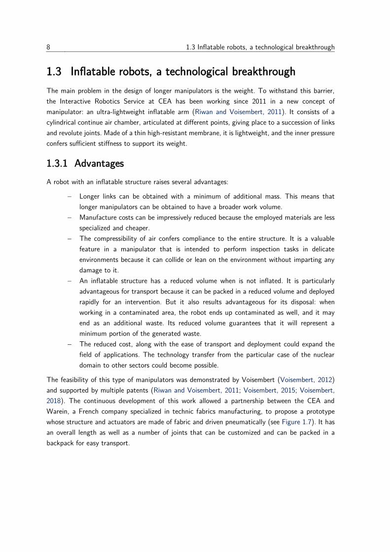
8 1.3 Inflatable robots, a technological breakthrough

1.3 Inflatable robots, a technological breakthrough

The main problem in the design of longer manipulators is the weight. To withstand this barrier,

the Interactive Robotics Service at CEA has been working since 2011 in a new concept of

manipulator: an ultra-lightweight inflatable arm (Riwan and Voisembert, 2011). It consists of a

cylindrical continue air chamber, articulated at different points, giving place to a succession of links

and revolute joints. Made of a thin high-resistant membrane, it is lightweight, and the inner pressure

confers sufficient stiffness to support its weight.

1.3.1 Advantages

A robot with an inflatable structure raises several advantages:

− Longer links can be obtained with a minimum of additional mass. This means that

longer manipulators can be obtained to have a broader work volume.

− Manufacture costs can be impressively reduced because the employed materials are less

specialized and cheaper.

− The compressibility of air confers compliance to the entire structure. It is a valuable

feature in a manipulator that is intended to perform inspection tasks in delicate

environments because it can collide or lean on the environment without imparting any

damage to it.

− An inflatable structure has a reduced volume when is not inflated. It is particularly

advantageous for transport because it can be packed in a reduced volume and deployed

rapidly for an intervention. But it also results advantageous for its disposal: when

working in a contaminated area, the robot ends up contaminated as well, and it may

end as an additional waste. Its reduced volume guarantees that it will represent a

minimum portion of the generated waste.

− The reduced cost, along with the ease of transport and deployment could expand the

field of applications. The technology transfer from the particular case of the nuclear

domain to other sectors could become possible.

The feasibility of this type of manipulators was demonstrated by Voisembert (Voisembert, 2012)

and supported by multiple patents (Riwan and Voisembert, 2011; Voisembert, 2015; Voisembert,

2018). The continuous development of this work allowed a partnership between the CEA and

Warein, a French company specialized in technic fabrics manufacturing, to propose a prototype

whose structure and actuators are made of fabric and driven pneumatically (see Figure 1.7). It has

an overall length as well as a number of joints that can be customized and can be packed in a

backpack for easy transport.

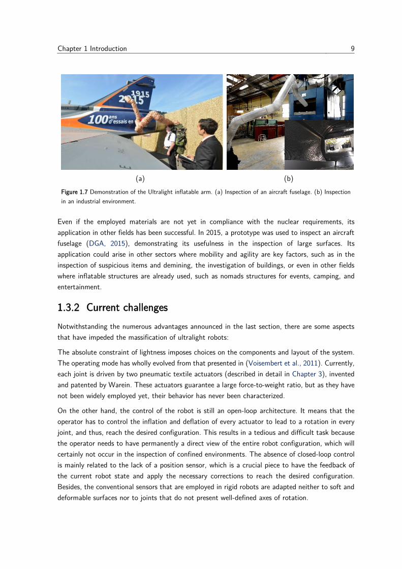
Chapter 1 Introduction 9

(a) (b)

Figure 1.7 Demonstration of the Ultralight inflatable arm. (a) Inspection of an aircraft fuselage. (b) Inspection

in an industrial environment.

Even if the employed materials are not yet in compliance with the nuclear requirements, its

application in other fields has been successful. In 2015, a prototype was used to inspect an aircraft

fuselage (DGA, 2015), demonstrating its usefulness in the inspection of large surfaces. Its

application could arise in other sectors where mobility and agility are key factors, such as in the

inspection of suspicious items and demining, the investigation of buildings, or even in other fields

where inflatable structures are already used, such as nomads structures for events, camping, and

entertainment.

1.3.2 Current challenges

Notwithstanding the numerous advantages announced in the last section, there are some aspects

that have impeded the massification of ultralight robots:

The absolute constraint of lightness imposes choices on the components and layout of the system.

The operating mode has wholly evolved from that presented in (Voisembert et al., 2011). Currently,

each joint is driven by two pneumatic textile actuators (described in detail in Chapter 3), invented

and patented by Warein. These actuators guarantee a large force-to-weight ratio, but as they have

not been widely employed yet, their behavior has never been characterized.

On the other hand, the control of the robot is still an open-loop architecture. It means that the

operator has to control the inflation and deflation of every actuator to lead to a rotation in every

joint, and thus, reach the desired configuration. This results in a tedious and difficult task because

the operator needs to have permanently a direct view of the entire robot configuration, which will

certainly not occur in the inspection of confined environments. The absence of closed-loop control

is mainly related to the lack of a position sensor, which is a crucial piece to have the feedback of

the current robot state and apply the necessary corrections to reach the desired configuration.

Besides, the conventional sensors that are employed in rigid robots are adapted neither to soft and

deformable surfaces nor to joints that do not present well-defined axes of rotation.

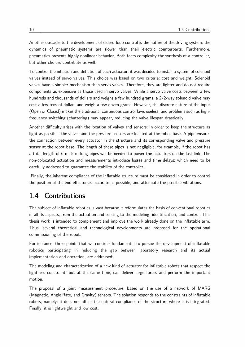
10 1.4 Contributions

Another obstacle to the development of closed-loop control is the nature of the driving system: the

dynamics of pneumatic systems are slower than their electric counterparts. Furthermore,

pneumatics presents highly nonlinear behavior. Both facts complexify the synthesis of a controller,

but other choices contribute as well:

To control the inflation and deflation of each actuator, it was decided to install a system of solenoid

valves instead of servo valves. This choice was based on two criteria: cost and weight. Solenoid

valves have a simpler mechanism than servo valves. Therefore, they are lighter and do not require

components as expensive as those used in servo valves. While a servo valve costs between a few

hundreds and thousands of dollars and weighs a few hundred grams, a 2/2-way solenoid valve may

cost a few tens of dollars and weigh a few dozen grams. However, the discrete nature of the input

(Open or Closed) makes the traditional continuous control laws useless, and problems such as high-

frequency switching (chattering) may appear, reducing the valve lifespan drastically.

Another difficulty arises with the location of valves and sensors: In order to keep the structure as

light as possible, the valves and the pressure sensors are located at the robot base. A pipe ensures

the connection between every actuator in the structure and its corresponding valve and pressure

sensor at the robot base. The length of these pipes is not negligible, for example, if the robot has

a total length of 6 m, 5 m long pipes will be needed to power the actuators on the last link. The

non-colocated actuation and measurements introduce losses and time delays; which need to be

carefully addressed to guarantee the stability of the controller.

Finally, the inherent compliance of the inflatable structure must be considered in order to control

the position of the end effector as accurate as possible, and attenuate the possible vibrations.

1.4 Contributions

The subject of inflatable robotics is vast because it reformulates the basis of conventional robotics

in all its aspects, from the actuation and sensing to the modeling, identification, and control. This

thesis work is intended to complement and improve the work already done on the inflatable arm.

Thus, several theoretical and technological developments are proposed for the operational

commissioning of the robot.

For instance, three points that we consider fundamental to pursue the development of inflatable

robotics participating in reducing the gap between laboratory research and its actual

implementation and operation, are addressed:

The modeling and characterization of a new kind of actuator for inflatable robots that respect the

lightness constraint, but at the same time, can deliver large forces and perform the important

motion.

The proposal of a joint measurement procedure, based on the use of a network of MARG

(Magnetic, Angle Rate, and Gravity) sensors. The solution responds to the constraints of inflatable

robots, namely: it does not affect the natural compliance of the structure where it is integrated.

Finally, it is lightweight and low cost.

Chapter 1 Introduction 11

This work led to two communications in conferences with review committee and one paper

submitted to a peer-reviewed journal:

J. M. Álvarez-Palacio, A. Riwan, N. Mechbal, E. Monteiro, and S. Voisembert. ‘A Novel Inflatable

Actuator for Inflatable Robotic Arms’. In 2017 IEEE International Conference on Advanced

Intelligent Mechatronics (AIM), 88–93, 2017.

J. M. Álvarez-Palacio, A. Riwan, N. Mechbal, E. Monteiro, and S. Voisembert. ‘A Novel Inflatable

Joint with Position Estimation Using Perturbed Magnetometers’. In 2019 IEEE/ASME

International Conference on Advanced Intelligent Mechatronics (AIM), 1133–38, 2019.

J. M. Álvarez-Palacio, A. Riwan, N. Mechbal, E. Monteiro, and S. Voisembert. ‘A Novel Inflatable

Actuator based on Simultaneous Eversion - Retraction’. Submitted to Soft Robotics, peer-reviewed

journal.

1.5 Outline

The organization of this thesis is described hereafter:

Chapter 2 presents a state of the art of inflatable structures, their advantages and current

applications. It takes a look of ongoing development in soft robotics, its advancements and current

challenges. Finally, it details the structure of the inflatable robot studied in this thesis and compares

its features with other existent robots found in the literature.

Chapter 3 starts with the state of the art of pneumatic actuators. Then, it describes the actuators

that are employed in every joint of the robot. First, a prototype with a cylindrical shape is presented,

detailing its working principle, a simplified study of its kinematics and force generation, as well as

the experimental characterization. A drawback of instability with this concept is introduced and

motivates the study of another concept with a conical shape. As in the first case, a geometric and

static study is carried on, and compared to experimental results. The simplified study does not

capture specific features related to properties of the material employed or the folds and wrinkles

that appear inexorably. This motivated the implementation of a finite elements analysis, which is

also presented as well as the simulation results.

Chapter 4 presents a state of the art of position sensors that have been proposed in other fields

and that may be useful in the context of soft and inflatable robotics. Then, the problem of articular

position measurement between two bodies is addressed through two approaches: The first one

estimates the angle between two bodies using a three-axis magnetometer fixed in one of the bodies

and perturbed by a permanent magnet fixed in the other one. This approach did not report

successful results, which motivated the exploration of a second approach, exploiting the measures

of additional sensors, namely, accelerometers and gyroscopes. This method is based on the

estimation of relative orientation between two bodies using corresponding vector measurements in

different frames. The mathematical background about the representations of rotations in the space

is described, giving particular importance to the representation through quaternions. This will set

12 1.5 Outline

the basis for the introduction of an algorithm for the estimation of relative orientation between

two bodies in the space.

Chapter 5 introduces the dynamic model of the actuation system, an approach to the position

control of one inflatable joint through a Sliding Mode Controller.

Finally, Chapter 6 presents the general conclusions of this research work and points out some

directions and suggestions to address potential future work.

Chapter 2

State of the art

Not to know what has been transacted in former

times is to be always a child. If no use is made

of the labors of past ages, the world must

remain always in the infancy of knowledge

― Marcus Tullius Cicero

Contents

2.1 Inflatable structures .......................................................................................... 14

2.1.1 Ground applications .................................................................................... 15

2.1.2 Aerospatial applications .............................................................................. 18

2.2 Soft robotics .................................................................................................... 23

2.2.1 Materials .................................................................................................... 23

2.2.2 Actuation ................................................................................................... 24

2.2.3 Structure .................................................................................................... 25

2.2.4 Applications ................................................................................................ 28

2.3 Ultra-light inflatable arm ................................................................................... 32

2.3.1 Complete structure ..................................................................................... 32

2.3.2 Joint .......................................................................................................... 33

2.3.3 Joint actuation ........................................................................................... 34

2.3.4 Inflatable actuator ...................................................................................... 35

2.4 Conclusions ...................................................................................................... 36

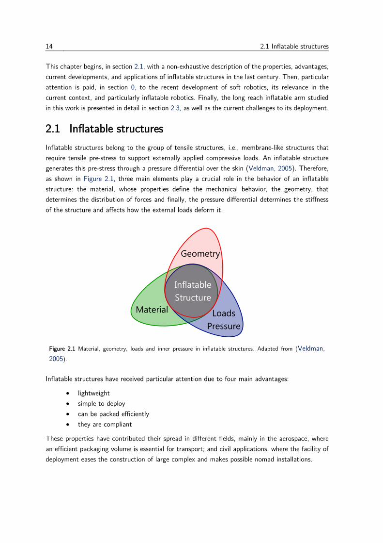
14 2.1 Inflatable structures

This chapter begins, in section 2.1, with a non-exhaustive description of the properties, advantages,

current developments, and applications of inflatable structures in the last century. Then, particular

attention is paid, in section 0, to the recent development of soft robotics, its relevance in the

current context, and particularly inflatable robotics. Finally, the long reach inflatable arm studied

in this work is presented in detail in section 2.3, as well as the current challenges to its deployment.

2.1 Inflatable structures

Inflatable structures belong to the group of tensile structures, i.e., membrane-like structures that

require tensile pre-stress to support externally applied compressive loads. An inflatable structure

generates this pre-stress through a pressure differential over the skin (Veldman, 2005). Therefore,

as shown in Figure 2.1, three main elements play a crucial role in the behavior of an inflatable

structure: the material, whose properties define the mechanical behavior, the geometry, that

determines the distribution of forces and finally, the pressure differential determines the stiffness

of the structure and affects how the external loads deform it.

Figure 2.1 Material, geometry, loads and inner pressure in inflatable structures. Adapted from (Veldman,

2005).

Inflatable structures have received particular attention due to four main advantages:

• lightweight

• simple to deploy

• can be packed efficiently

• they are compliant

These properties have contributed their spread in different fields, mainly in the aerospace, where

an efficient packaging volume is essential for transport; and civil applications, where the facility of

deployment eases the construction of large complex and makes possible nomad installations.

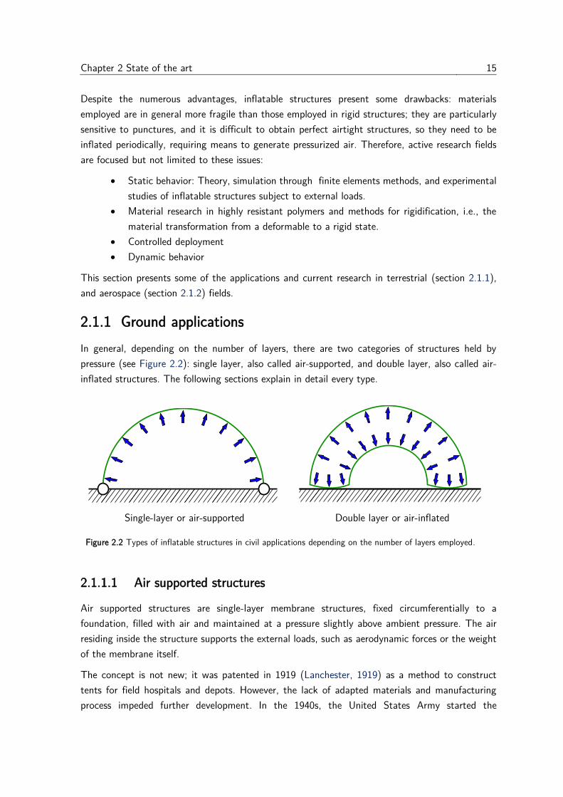
Chapter 2 State of the art 15

Despite the numerous advantages, inflatable structures present some drawbacks: materials

employed are in general more fragile than those employed in rigid structures; they are particularly

sensitive to punctures, and it is difficult to obtain perfect airtight structures, so they need to be

inflated periodically, requiring means to generate pressurized air. Therefore, active research fields

are focused but not limited to these issues:

• Static behavior: Theory, simulation through finite elements methods, and experimental

studies of inflatable structures subject to external loads.

• Material research in highly resistant polymers and methods for rigidification, i.e., the

material transformation from a deformable to a rigid state.

• Controlled deployment

• Dynamic behavior

This section presents some of the applications and current research in terrestrial (section 2.1.1),

and aerospace (section 2.1.2) fields.

2.1.1 Ground applications

In general, depending on the number of layers, there are two categories of structures held by

pressure (see Figure 2.2): single layer, also called air-supported, and double layer, also called air-

inflated structures. The following sections explain in detail every type.

Single-layer or air-supported Double layer or air-inflated

Figure 2.2 Types of inflatable structures in civil applications depending on the number of layers employed.

2.1.1.1 Air supported structures

Air supported structures are single-layer membrane structures, fixed circumferentially to a

foundation, filled with air and maintained at a pressure slightly above ambient pressure. The air

residing inside the structure supports the external loads, such as aerodynamic forces or the weight

of the membrane itself.

The concept is not new; it was patented in 1919 (Lanchester, 1919) as a method to construct

tents for field hospitals and depots. However, the lack of adapted materials and manufacturing

process impeded further development. In the 1940s, the United States Army started the

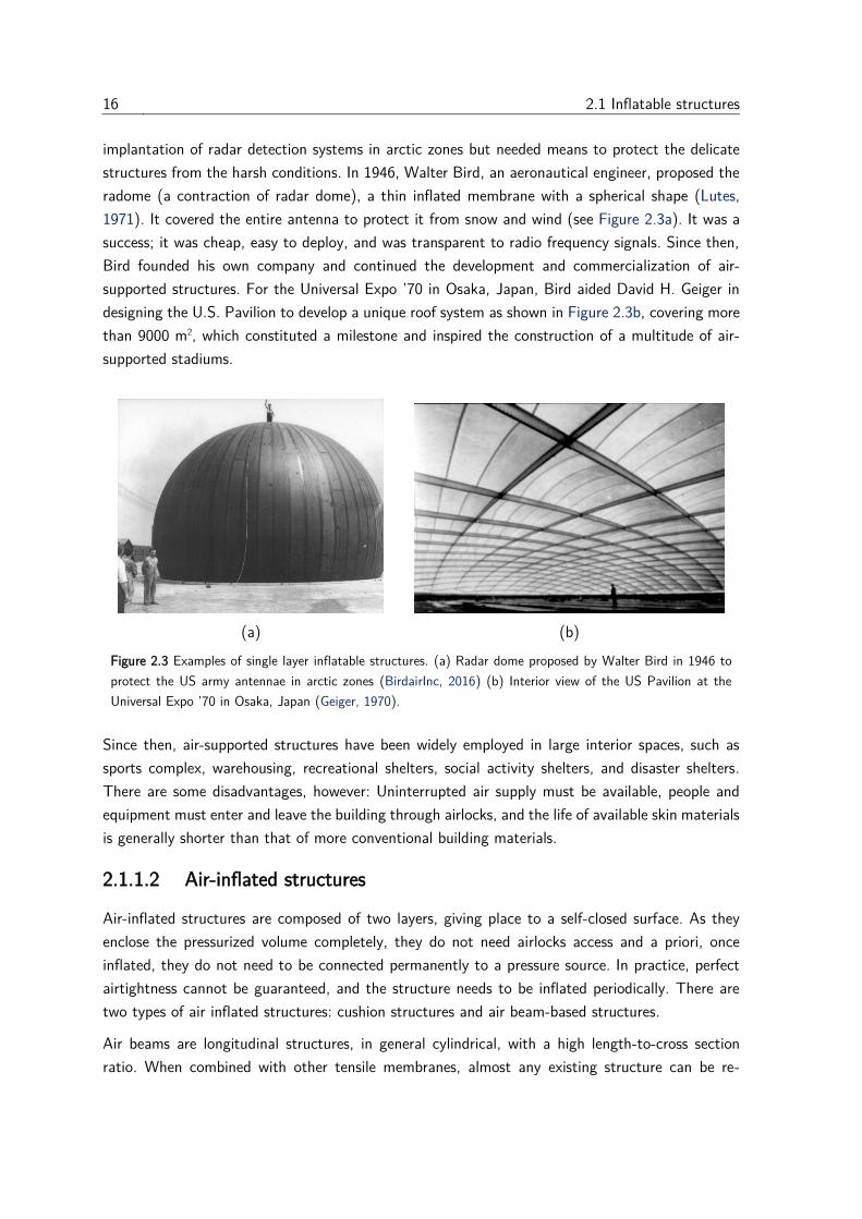
16 2.1 Inflatable structures

implantation of radar detection systems in arctic zones but needed means to protect the delicate

structures from the harsh conditions. In 1946, Walter Bird, an aeronautical engineer, proposed the

radome (a contraction of radar dome), a thin inflated membrane with a spherical shape (Lutes,

1971). It covered the entire antenna to protect it from snow and wind (see Figure 2.3a). It was a

success; it was cheap, easy to deploy, and was transparent to radio frequency signals. Since then,

Bird founded his own company and continued the development and commercialization of air-

supported structures. For the Universal Expo ’70 in Osaka, Japan, Bird aided David H. Geiger in

designing the U.S. Pavilion to develop a unique roof system as shown in Figure 2.3b, covering more

than 9000 m2, which constituted a milestone and inspired the construction of a multitude of air-

supported stadiums.

(a) (b)

Figure 2.3 Examples of single layer inflatable structures. (a) Radar dome proposed by Walter Bird in 1946 to

protect the US army antennae in arctic zones (BirdairInc, 2016) (b) Interior view of the US Pavilion at the

Universal Expo ’70 in Osaka, Japan (Geiger, 1970).

Since then, air-supported structures have been widely employed in large interior spaces, such as

sports complex, warehousing, recreational shelters, social activity shelters, and disaster shelters.

There are some disadvantages, however: Uninterrupted air supply must be available, people and

equipment must enter and leave the building through airlocks, and the life of available skin materials

is generally shorter than that of more conventional building materials.

2.1.1.2 Air-inflated structures

Air-inflated structures are composed of two layers, giving place to a self-closed surface. As they

enclose the pressurized volume completely, they do not need airlocks access and a priori, once

inflated, they do not need to be connected permanently to a pressure source. In practice, perfect

airtightness cannot be guaranteed, and the structure needs to be inflated periodically. There are

two types of air inflated structures: cushion structures and air beam-based structures.

Air beams are longitudinal structures, in general cylindrical, with a high length-to-cross section

ratio. When combined with other tensile membranes, almost any existing structure can be re-

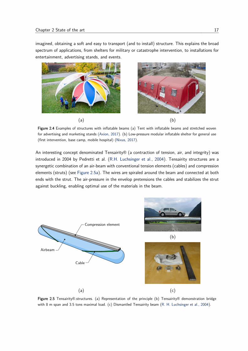
Chapter 2 State of the art 17

imagined, obtaining a soft and easy to transport (and to install) structure. This explains the broad

spectrum of applications, from shelters for military or catastrophe intervention, to installations for

entertainment, advertising stands, and events.

(a) (b)

Figure 2.4 Examples of structures with inflatable beams (a) Tent with inflatable beams and stretched woven

for advertising and marketing stands (Axion, 2017). (b) Low-pressure modular inflatable shelter for general use

(first intervention, base camp, mobile hospital) (Nixus, 2017).

An interesting concept denominated Tensairity® (a contraction of tension, air, and integrity) was

introduced in 2004 by Pedretti et al. (R.H. Luchsinger et al., 2004). Tensairity structures are a

synergetic combination of an air-beam with conventional tension elements (cables) and compression

elements (struts) (see Figure 2.5a). The wires are spiraled around the beam and connected at both

ends with the strut. The air-pressure in the envelop pretensions the cables and stabilizes the strut

against buckling, enabling optimal use of the materials in the beam.

(b)

(a) (c)

Figure 2.5 Tensairity®.structures. (a) Representation of the principle (b) Tensairity® demonstration bridge

with 8 m span and 3.5 tons maximal load. (c) Dismantled Tensairity beam (R. H. Luchsinger et al., 2004).

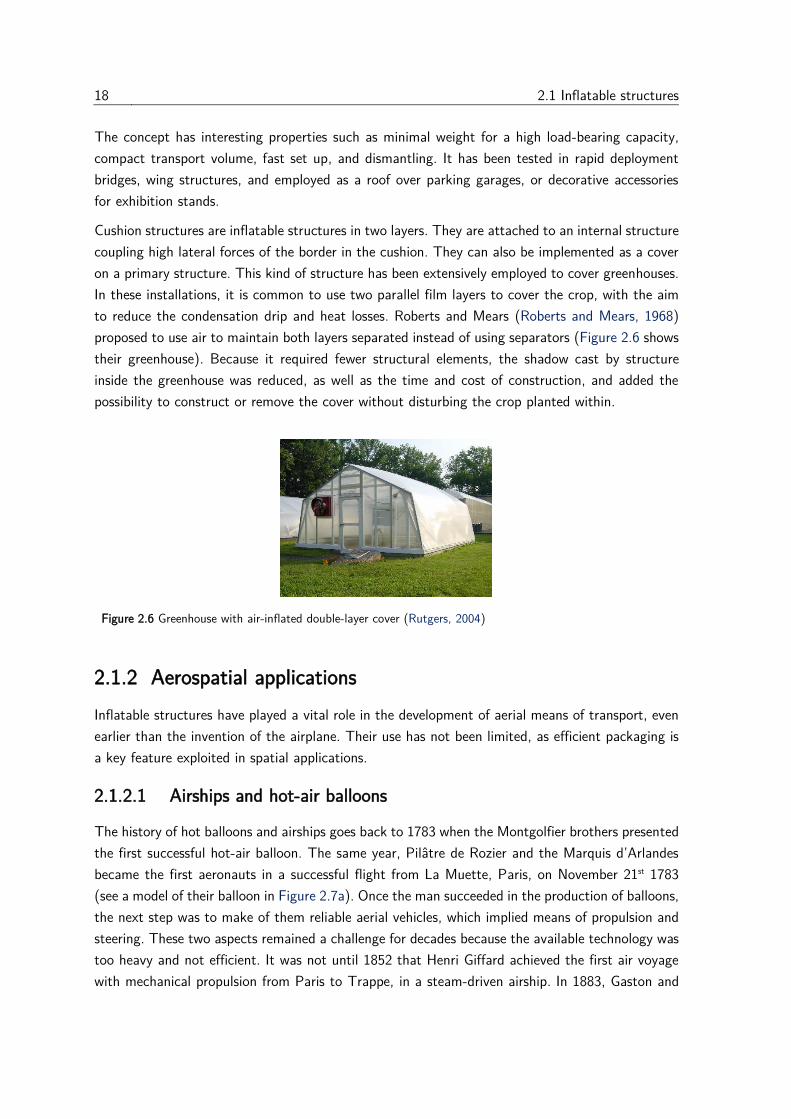
18 2.1 Inflatable structures

The concept has interesting properties such as minimal weight for a high load-bearing capacity,

compact transport volume, fast set up, and dismantling. It has been tested in rapid deployment

bridges, wing structures, and employed as a roof over parking garages, or decorative accessories

for exhibition stands.

Cushion structures are inflatable structures in two layers. They are attached to an internal structure

coupling high lateral forces of the border in the cushion. They can also be implemented as a cover

on a primary structure. This kind of structure has been extensively employed to cover greenhouses.

In these installations, it is common to use two parallel film layers to cover the crop, with the aim

to reduce the condensation drip and heat losses. Roberts and Mears (Roberts and Mears, 1968)

proposed to use air to maintain both layers separated instead of using separators (Figure 2.6 shows

their greenhouse). Because it required fewer structural elements, the shadow cast by structure

inside the greenhouse was reduced, as well as the time and cost of construction, and added the

possibility to construct or remove the cover without disturbing the crop planted within.

Figure 2.6 Greenhouse with air-inflated double-layer cover (Rutgers, 2004)

2.1.2 Aerospatial applications

Inflatable structures have played a vital role in the development of aerial means of transport, even

earlier than the invention of the airplane. Their use has not been limited, as efficient packaging is

a key feature exploited in spatial applications.

2.1.2.1 Airships and hot-air balloons

The history of hot balloons and airships goes back to 1783 when the Montgolfier brothers presented

the first successful hot-air balloon. The same year, Pilâtre de Rozier and the Marquis d’Arlandes

became the first aeronauts in a successful flight from La Muette, Paris, on November 21st 1783

(see a model of their balloon in Figure 2.7a). Once the man succeeded in the production of balloons,

the next step was to make of them reliable aerial vehicles, which implied means of propulsion and

steering. These two aspects remained a challenge for decades because the available technology was

too heavy and not efficient. It was not until 1852 that Henri Giffard achieved the first air voyage

with mechanical propulsion from Paris to Trappe, in a steam-driven airship. In 1883, Gaston and

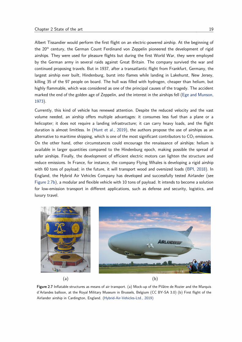
Chapter 2 State of the art 19

Albert Tissandier would perform the first flight on an electric-powered airship. At the beginning of

the 20th century, the German Count Ferdinand von Zeppelin pioneered the development of rigid

airships. They were used for pleasure flights but during the first World War, they were employed

by the German army in several raids against Great Britain. The company survived the war and

continued proposing travels. But in 1937, after a transatlantic flight from Frankfurt, Germany, the

largest airship ever built, Hindenburg, burst into flames while landing in Lakehurst, New Jersey,

killing 35 of the 97 people on board. The hull was filled with hydrogen, cheaper than helium, but

highly flammable, which was considered as one of the principal causes of the tragedy. The accident

marked the end of the golden age of Zeppelin, and the interest in the airships fell (Ege and Munson,

1973).

Currently, this kind of vehicle has renewed attention. Despite the reduced velocity and the vast

volume needed, an airship offers multiple advantages: it consumes less fuel than a plane or a

helicopter; it does not require a landing infrastructure; it can carry heavy loads, and the flight

duration is almost limitless. In (Hunt et al., 2019), the authors propose the use of airships as an

alternative to maritime shipping, which is one of the most significant contributors to CO2 emissions.

On the other hand, other circumstances could encourage the renaissance of airships: helium is

available in larger quantities compared to the Hindenburg epoch, making possible the spread of

safer airships. Finally, the development of efficient electric motors can lighten the structure and

reduce emissions. In France, for instance, the company Flying Whales is developing a rigid airship

with 60 tons of payload; in the future, it will transport wood and oversized loads (BPI, 2018). In

England, the Hybrid Air Vehicles Company has developed and successfully tested Airlander (see

Figure 2.7b), a modular and flexible vehicle with 10 tons of payload. It intends to become a solution

for low-emission transport in different applications, such as defense and security, logistics, and

luxury travel.

(a) (b)

Figure 2.7 Inflatable structures as means of air transport. (a) Mock-up of the Pilâtre de Rozier and the Marquis

d’Arlandes balloon, at the Royal Military Museum in Brussels, Belgium (CC BY-SA 3.0) (b) First flight of the

Airlander airship in Cardington, England. (Hybrid-Air-Vehicles-Ltd., 2019)

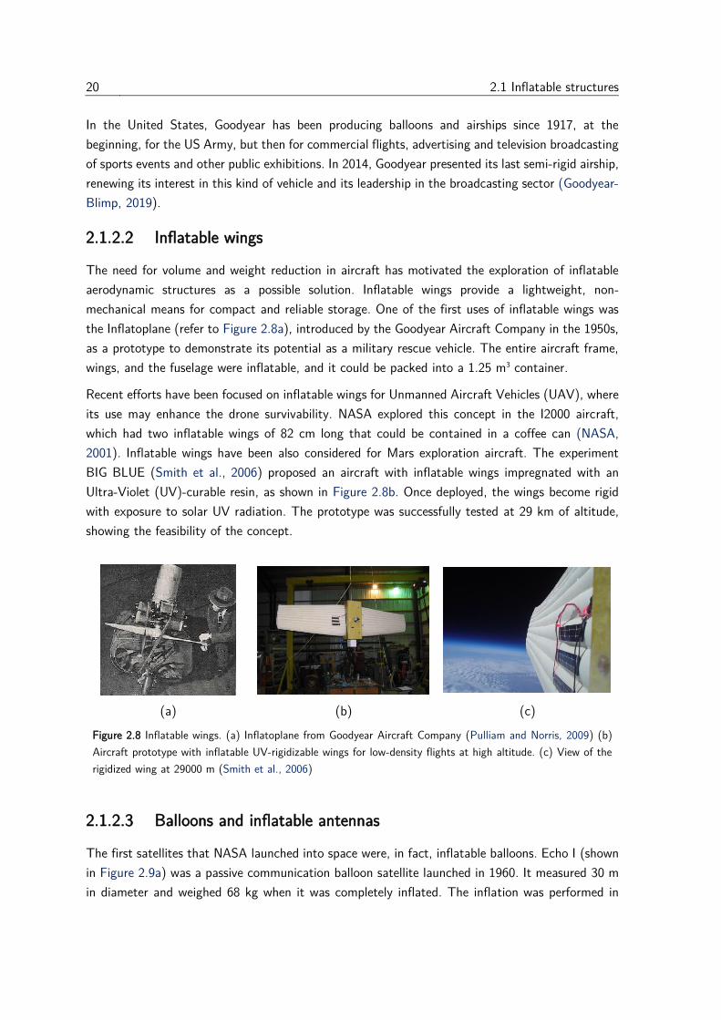
20 2.1 Inflatable structures

In the United States, Goodyear has been producing balloons and airships since 1917, at the

beginning, for the US Army, but then for commercial flights, advertising and television broadcasting

of sports events and other public exhibitions. In 2014, Goodyear presented its last semi-rigid airship,

renewing its interest in this kind of vehicle and its leadership in the broadcasting sector (Goodyear-

Blimp, 2019).

2.1.2.2 Inflatable wings

The need for volume and weight reduction in aircraft has motivated the exploration of inflatable

aerodynamic structures as a possible solution. Inflatable wings provide a lightweight, non-

mechanical means for compact and reliable storage. One of the first uses of inflatable wings was

the Inflatoplane (refer to Figure 2.8a), introduced by the Goodyear Aircraft Company in the 1950s,

as a prototype to demonstrate its potential as a military rescue vehicle. The entire aircraft frame,

wings, and the fuselage were inflatable, and it could be packed into a 1.25 m3 container.

Recent efforts have been focused on inflatable wings for Unmanned Aircraft Vehicles (UAV), where

its use may enhance the drone survivability. NASA explored this concept in the I2000 aircraft,

which had two inflatable wings of 82 cm long that could be contained in a coffee can (NASA,

2001). Inflatable wings have been also considered for Mars exploration aircraft. The experiment

BIG BLUE (Smith et al., 2006) proposed an aircraft with inflatable wings impregnated with an

Ultra-Violet (UV)-curable resin, as shown in Figure 2.8b. Once deployed, the wings become rigid

with exposure to solar UV radiation. The prototype was successfully tested at 29 km of altitude,

showing the feasibility of the concept.

(a) (b) (c)

Figure 2.8 Inflatable wings. (a) Inflatoplane from Goodyear Aircraft Company (Pulliam and Norris, 2009) (b)

Aircraft prototype with inflatable UV-rigidizable wings for low-density flights at high altitude. (c) View of the

rigidized wing at 29000 m (Smith et al., 2006)

2.1.2.3 Balloons and inflatable antennas

The first satellites that NASA launched into space were, in fact, inflatable balloons. Echo I (shown

in Figure 2.9a) was a passive communication balloon satellite launched in 1960. It measured 30 m

in diameter and weighed 68 kg when it was completely inflated. The inflation was performed in

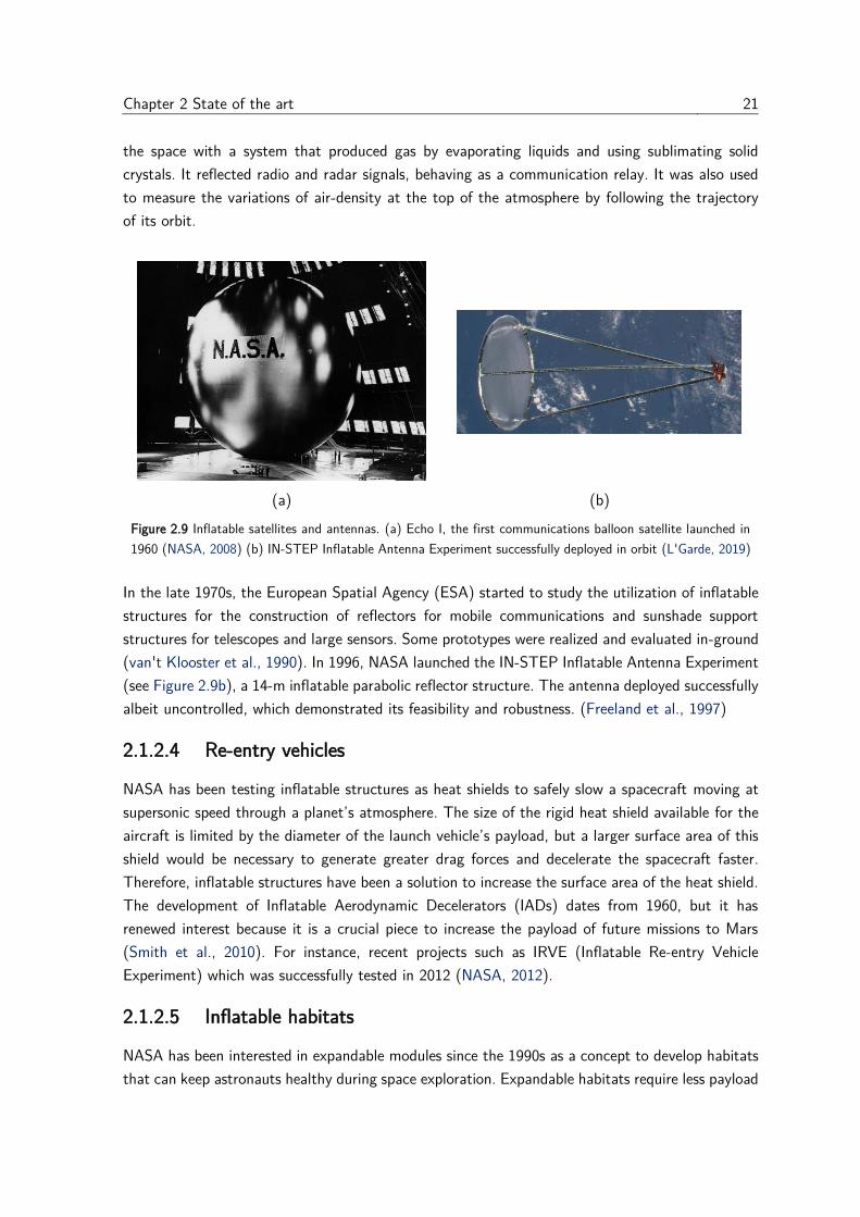
Chapter 2 State of the art 21

the space with a system that produced gas by evaporating liquids and using sublimating solid

crystals. It reflected radio and radar signals, behaving as a communication relay. It was also used

to measure the variations of air-density at the top of the atmosphere by following the trajectory

of its orbit.

(a) (b)

Figure 2.9 Inflatable satellites and antennas. (a) Echo I, the first communications balloon satellite launched in

1960 (NASA, 2008) (b) IN-STEP Inflatable Antenna Experiment successfully deployed in orbit (L'Garde, 2019)

In the late 1970s, the European Spatial Agency (ESA) started to study the utilization of inflatable

structures for the construction of reflectors for mobile communications and sunshade support

structures for telescopes and large sensors. Some prototypes were realized and evaluated in-ground

(van't Klooster et al., 1990). In 1996, NASA launched the IN-STEP Inflatable Antenna Experiment

(see Figure 2.9b), a 14-m inflatable parabolic reflector structure. The antenna deployed successfully

albeit uncontrolled, which demonstrated its feasibility and robustness. (Freeland et al., 1997)

2.1.2.4 Re-entry vehicles

NASA has been testing inflatable structures as heat shields to safely slow a spacecraft moving at

supersonic speed through a planet’s atmosphere. The size of the rigid heat shield available for the

aircraft is limited by the diameter of the launch vehicle’s payload, but a larger surface area of this

shield would be necessary to generate greater drag forces and decelerate the spacecraft faster.

Therefore, inflatable structures have been a solution to increase the surface area of the heat shield.

The development of Inflatable Aerodynamic Decelerators (IADs) dates from 1960, but it has

renewed interest because it is a crucial piece to increase the payload of future missions to Mars

(Smith et al., 2010). For instance, recent projects such as IRVE (Inflatable Re-entry Vehicle

Experiment) which was successfully tested in 2012 (NASA, 2012).

2.1.2.5 Inflatable habitats

NASA has been interested in expandable modules since the 1990s as a concept to develop habitats

that can keep astronauts healthy during space exploration. Expandable habitats require less payload

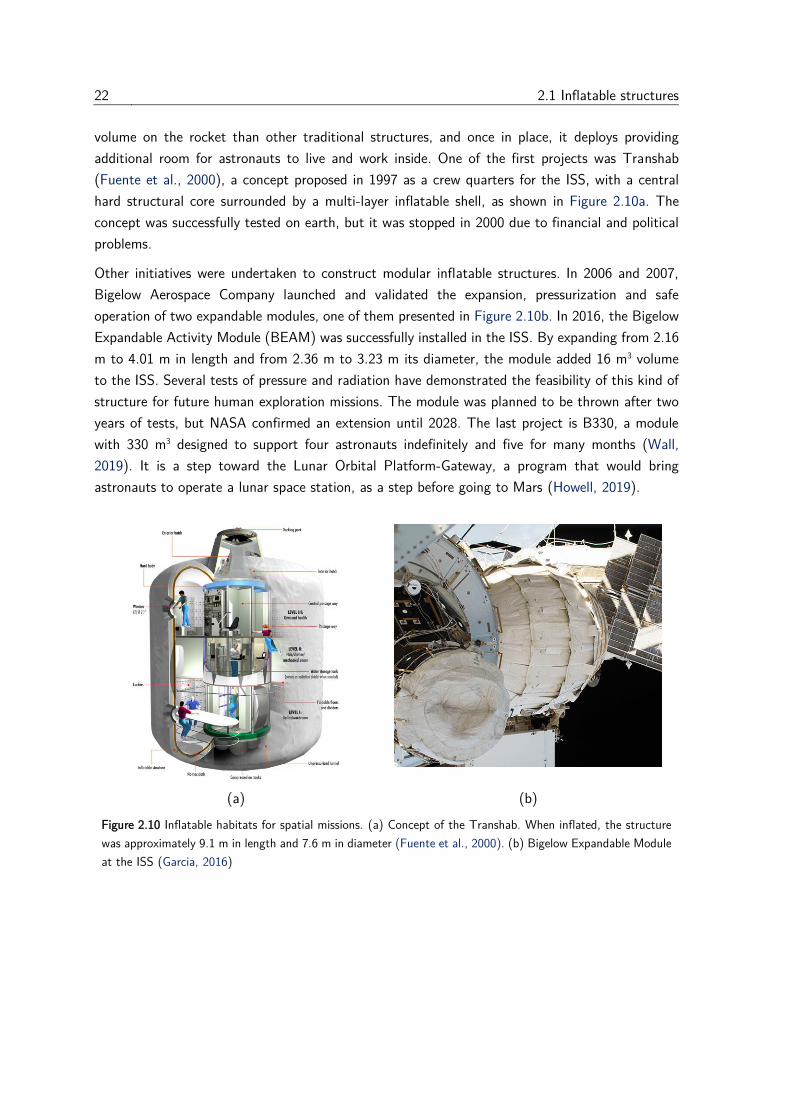
22 2.1 Inflatable structures

volume on the rocket than other traditional structures, and once in place, it deploys providing

additional room for astronauts to live and work inside. One of the first projects was Transhab

(Fuente et al., 2000), a concept proposed in 1997 as a crew quarters for the ISS, with a central

hard structural core surrounded by a multi-layer inflatable shell, as shown in Figure 2.10a. The

concept was successfully tested on earth, but it was stopped in 2000 due to financial and political

problems.

Other initiatives were undertaken to construct modular inflatable structures. In 2006 and 2007,

Bigelow Aerospace Company launched and validated the expansion, pressurization and safe

operation of two expandable modules, one of them presented in Figure 2.10b. In 2016, the Bigelow

Expandable Activity Module (BEAM) was successfully installed in the ISS. By expanding from 2.16

m to 4.01 m in length and from 2.36 m to 3.23 m its diameter, the module added 16 m3 volume

to the ISS. Several tests of pressure and radiation have demonstrated the feasibility of this kind of

structure for future human exploration missions. The module was planned to be thrown after two

years of tests, but NASA confirmed an extension until 2028. The last project is B330, a module

with 330 m3 designed to support four astronauts indefinitely and five for many months (Wall,

2019). It is a step toward the Lunar Orbital Platform-Gateway, a program that would bring

astronauts to operate a lunar space station, as a step before going to Mars (Howell, 2019).

(a) (b)

Figure 2.10 Inflatable habitats for spatial missions. (a) Concept of the Transhab. When inflated, the structure

was approximately 9.1 m in length and 7.6 m in diameter (Fuente et al., 2000). (b) Bigelow Expandable Module

at the ISS (Garcia, 2016)

Chapter 2 State of the art 23

2.2 Soft robotics

One of the advantages of inflatable structures mentioned at the beginning of the last section is

their intrinsic compliance. The ability to adapt the shape to the applied forces has been a catalyst

in recent developments, and particularly, soft robotics.

What does it mean “soft”? It may be a relative concept; a piece of steel may be considered soft

compared to a diamond, whereas it will be regarded as rigid in other situations, all depend on what

is compared to. The concept of “soft” or “rigid” is related to a property of materials, the elastic

modulus, that can be measured and compared. The elastic modulus describes the force needed to

induce a reversible deformation of the material. In the robotics context, the question is addressed

from the point of view of human-robot interaction. Therefore, the term “soft” is applied to

materials whose elastic module is in the range of that of biological tissues. Soft robots are defined

as systems capable of autonomous behavior, that are primarily composed of materials with moduli

in the interval of that of soft organic materials. (Rus and Tolley, 2015).

Although soft robotics is a relatively young field of research, it has become in the last years a

trending topic in the science community, because it opens a path to versatile robots that can adapt

easily to different environments and tasks, unlike conventional robots with rigid bodies that are

excellent in well-defined tasks but difficult to adjust to new situations (Trimmer, 2013).

It also aims to relieve some of the complexity of robot control, introducing intelligence on the

hardware side. It means that a significant part of the motion programming is already “coded” in

the robot design, obtaining natural movements and adapted shapes that are highly difficult to

achieve even with accurate sensors and advanced control algorithms.

2.2.1 Materials

As pointed out before, soft robots are made of materials whose elastic modulus is similar to that

of biological tissues. Figure 2.11 presents the elastic modulus of different biological and synthetic

materials. In general, materials such as rubber, silicone elastomer, polyethylene, have an elastic

modulus below 1 GPa and exhibit considerable compliance under normal loading conditions.

The availability of advanced organic elastomers with low elastic moduli and high extensibility has

become really effective recently. Materials such as metals or ceramics were well known in ancient

civilizations, but extensible materials, e.g., natural rubber, even if it is ancient, it was not vulcanized

into a resilient rubber until the 19th century, and the properties are still not appropriate for soft

structures (Polygerinos et al., 2017). Recent advances in the synthesis and characterization of

elastomeric polymers such as siloxane-based polymers (especially polydimethylsiloxane (PDMS)

(Lötters et al., 1997) have allowed their wide adoption in soft lithography, microfluidics, and soft

robotics.

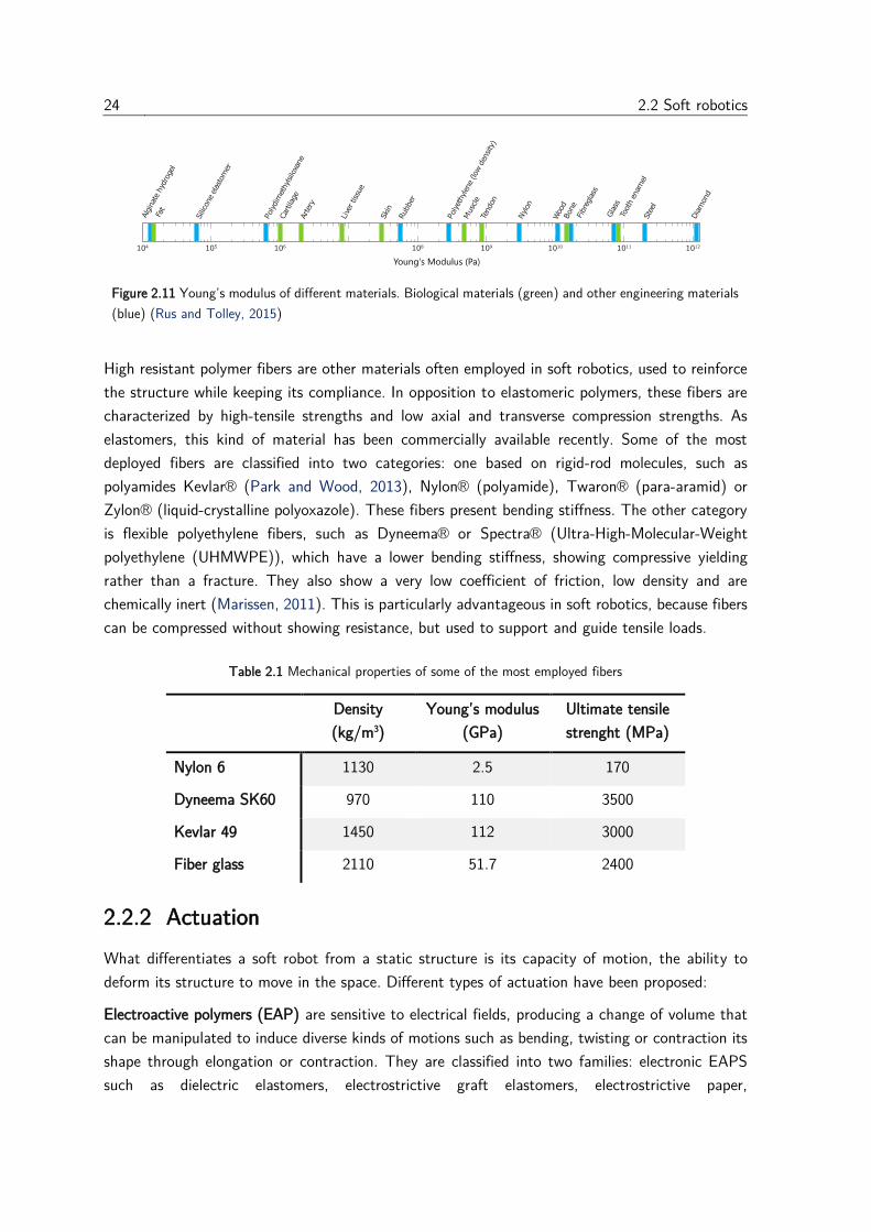
24 2.2 Soft robotics

Figure 2.11 Young’s modulus of different materials. Biological materials (green) and other engineering materials

(blue) (Rus and Tolley, 2015)

High resistant polymer fibers are other materials often employed in soft robotics, used to reinforce

the structure while keeping its compliance. In opposition to elastomeric polymers, these fibers are

characterized by high-tensile strengths and low axial and transverse compression strengths. As

elastomers, this kind of material has been commercially available recently. Some of the most

deployed fibers are classified into two categories: one based on rigid-rod molecules, such as

polyamides Kevlar® (Park and Wood, 2013), Nylon® (polyamide), Twaron® (para-aramid) or

Zylon® (liquid-crystalline polyoxazole). These fibers present bending stiffness. The other category

is flexible polyethylene fibers, such as Dyneema® or Spectra® (Ultra-High-Molecular-Weight

polyethylene (UHMWPE)), which have a lower bending stiffness, showing compressive yielding

rather than a fracture. They also show a very low coefficient of friction, low density and are

chemically inert (Marissen, 2011). This is particularly advantageous in soft robotics, because fibers

can be compressed without showing resistance, but used to support and guide tensile loads.

Table 2.1 Mechanical properties of some of the most employed fibers

Density

(kg/m3)

Young’s modulus

(GPa)

Ultimate tensile

strenght (MPa)

Nylon 6 1130 2.5 170

Dyneema SK60 970 110 3500

Kevlar 49 1450 112 3000

Fiber glass 2110 51.7 2400

2.2.2 Actuation

What differentiates a soft robot from a static structure is its capacity of motion, the ability to

deform its structure to move in the space. Different types of actuation have been proposed:

Electroactive polymers (EAP) are sensitive to electrical fields, producing a change of volume that

can be manipulated to induce diverse kinds of motions such as bending, twisting or contraction its

shape through elongation or contraction. They are classified into two families: electronic EAPS

such as dielectric elastomers, electrostrictive graft elastomers, electrostrictive paper,

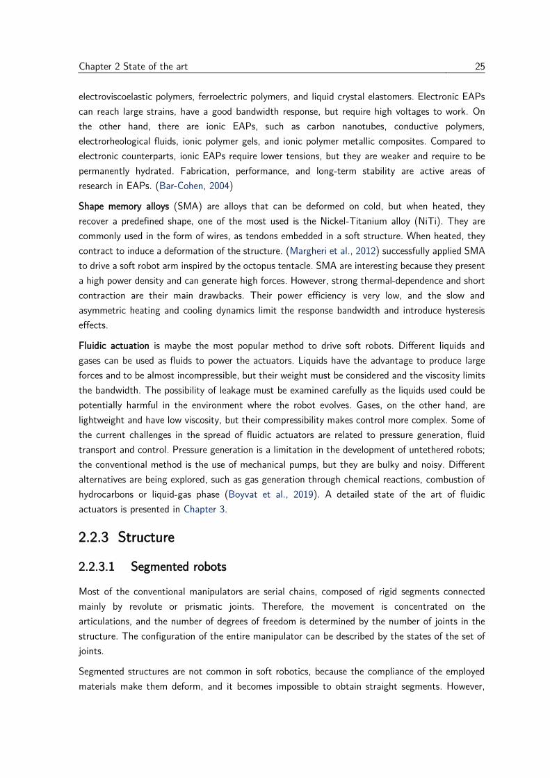
Chapter 2 State of the art 25

electroviscoelastic polymers, ferroelectric polymers, and liquid crystal elastomers. Electronic EAPs

can reach large strains, have a good bandwidth response, but require high voltages to work. On

the other hand, there are ionic EAPs, such as carbon nanotubes, conductive polymers,

electrorheological fluids, ionic polymer gels, and ionic polymer metallic composites. Compared to

electronic counterparts, ionic EAPs require lower tensions, but they are weaker and require to be

permanently hydrated. Fabrication, performance, and long-term stability are active areas of

research in EAPs. (Bar-Cohen, 2004)

Shape memory alloys (SMA) are alloys that can be deformed on cold, but when heated, they

recover a predefined shape, one of the most used is the Nickel-Titanium alloy (NiTi). They are

commonly used in the form of wires, as tendons embedded in a soft structure. When heated, they

contract to induce a deformation of the structure. (Margheri et al., 2012) successfully applied SMA

to drive a soft robot arm inspired by the octopus tentacle. SMA are interesting because they present

a high power density and can generate high forces. However, strong thermal-dependence and short

contraction are their main drawbacks. Their power efficiency is very low, and the slow and

asymmetric heating and cooling dynamics limit the response bandwidth and introduce hysteresis

effects.

Fluidic actuation is maybe the most popular method to drive soft robots. Different liquids and

gases can be used as fluids to power the actuators. Liquids have the advantage to produce large

forces and to be almost incompressible, but their weight must be considered and the viscosity limits

the bandwidth. The possibility of leakage must be examined carefully as the liquids used could be

potentially harmful in the environment where the robot evolves. Gases, on the other hand, are

lightweight and have low viscosity, but their compressibility makes control more complex. Some of

the current challenges in the spread of fluidic actuators are related to pressure generation, fluid

transport and control. Pressure generation is a limitation in the development of untethered robots;

the conventional method is the use of mechanical pumps, but they are bulky and noisy. Different

alternatives are being explored, such as gas generation through chemical reactions, combustion of

hydrocarbons or liquid-gas phase (Boyvat et al., 2019). A detailed state of the art of fluidic

actuators is presented in Chapter 3.

2.2.3 Structure

2.2.3.1 Segmented robots

Most of the conventional manipulators are serial chains, composed of rigid segments connected

mainly by revolute or prismatic joints. Therefore, the movement is concentrated on the

articulations, and the number of degrees of freedom is determined by the number of joints in the

structure. The configuration of the entire manipulator can be described by the states of the set of

joints.

Segmented structures are not common in soft robotics, because the compliance of the employed

materials make them deform, and it becomes impossible to obtain straight segments. However,

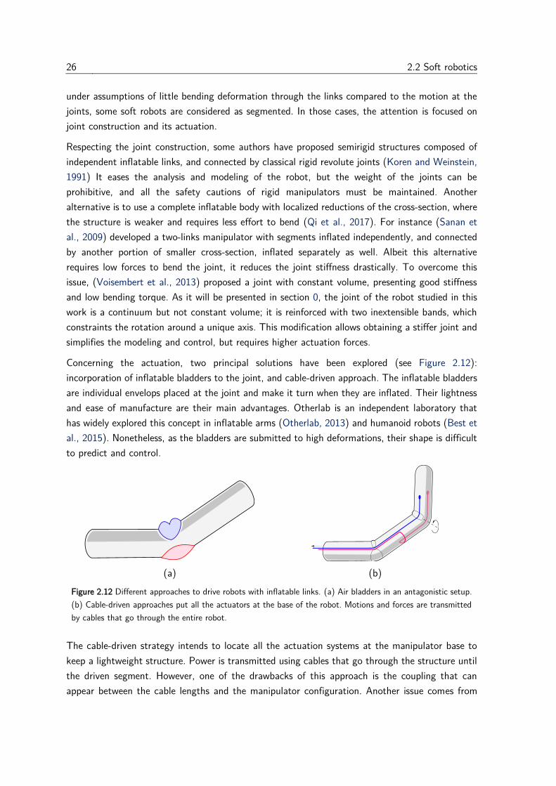
26 2.2 Soft robotics

under assumptions of little bending deformation through the links compared to the motion at the

joints, some soft robots are considered as segmented. In those cases, the attention is focused on

joint construction and its actuation.

Respecting the joint construction, some authors have proposed semirigid structures composed of

independent inflatable links, and connected by classical rigid revolute joints (Koren and Weinstein,

1991) It eases the analysis and modeling of the robot, but the weight of the joints can be

prohibitive, and all the safety cautions of rigid manipulators must be maintained. Another

alternative is to use a complete inflatable body with localized reductions of the cross-section, where

the structure is weaker and requires less effort to bend (Qi et al., 2017). For instance (Sanan et

al., 2009) developed a two-links manipulator with segments inflated independently, and connected

by another portion of smaller cross-section, inflated separately as well. Albeit this alternative

requires low forces to bend the joint, it reduces the joint stiffness drastically. To overcome this

issue, (Voisembert et al., 2013) proposed a joint with constant volume, presenting good stiffness

and low bending torque. As it will be presented in section 0, the joint of the robot studied in this

work is a continuum but not constant volume; it is reinforced with two inextensible bands, which

constraints the rotation around a unique axis. This modification allows obtaining a stiffer joint and

simplifies the modeling and control, but requires higher actuation forces.

Concerning the actuation, two principal solutions have been explored (see Figure 2.12):

incorporation of inflatable bladders to the joint, and cable-driven approach. The inflatable bladders

are individual envelops placed at the joint and make it turn when they are inflated. Their lightness

and ease of manufacture are their main advantages. Otherlab is an independent laboratory that

has widely explored this concept in inflatable arms (Otherlab, 2013) and humanoid robots (Best et

al., 2015). Nonetheless, as the bladders are submitted to high deformations, their shape is difficult

to predict and control.

(a) (b)

Figure 2.12 Different approaches to drive robots with inflatable links. (a) Air bladders in an antagonistic setup.

(b) Cable-driven approaches put all the actuators at the base of the robot. Motions and forces are transmitted

by cables that go through the entire robot.

The cable-driven strategy intends to locate all the actuation systems at the manipulator base to

keep a lightweight structure. Power is transmitted using cables that go through the structure until

the driven segment. However, one of the drawbacks of this approach is the coupling that can

appear between the cable lengths and the manipulator configuration. Another issue comes from

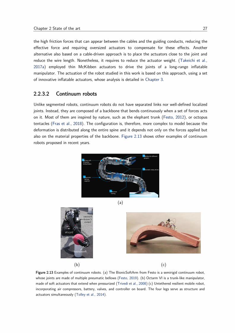
Chapter 2 State of the art 27

the high friction forces that can appear between the cables and the guiding conducts, reducing the

effective force and requiring oversized actuators to compensate for these effects. Another

alternative also based on a cable-driven approach is to place the actuators close to the joint and

reduce the wire length. Nonetheless, it requires to reduce the actuator weight. (Takeichi et al.,

2017a) employed thin McKibben actuators to drive the joints of a long-range inflatable

manipulator. The actuation of the robot studied in this work is based on this approach, using a set

of innovative inflatable actuators, whose analysis is detailed in Chapter 3.

2.2.3.2 Continuum robots

Unlike segmented robots, continuum robots do not have separated links nor well-defined localized

joints. Instead, they are composed of a backbone that bends continuously when a set of forces acts

on it. Most of them are inspired by nature, such as the elephant trunk (Festo, 2012), or octopus

tentacles (Fras et al., 2018). The configuration is, therefore, more complex to model because the

deformation is distributed along the entire spine and it depends not only on the forces applied but

also on the material properties of the backbone. Figure 2.13 shows other examples of continuum

robots proposed in recent years.

(a)

(b) (c)

Figure 2.13 Examples of continuum robots. (a) The BionicSoftArm from Festo is a semirigid continuum robot,

whose joints are made of multiple pneumatic bellows (Festo, 2019). (b) Octarm VI is a trunk-like manipulator,

made of soft actuators that extend when pressurized (Trivedi et al., 2008) (c) Untethered resilient mobile robot,

incorporating air compressors, battery, valves, and controller on board. The four legs serve as structure and

actuators simultaneously (Tolley et al., 2014).

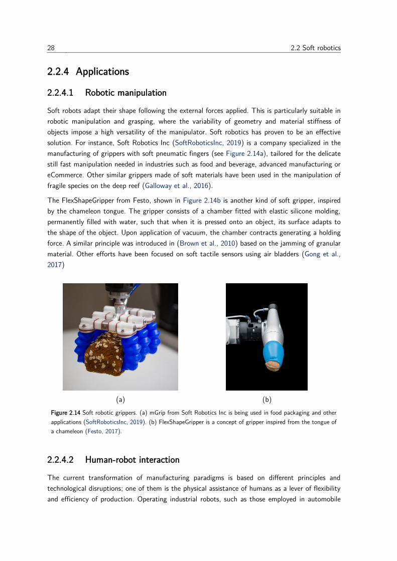
28 2.2 Soft robotics

2.2.4 Applications

2.2.4.1 Robotic manipulation

Soft robots adapt their shape following the external forces applied. This is particularly suitable in

robotic manipulation and grasping, where the variability of geometry and material stiffness of

objects impose a high versatility of the manipulator. Soft robotics has proven to be an effective

solution. For instance, Soft Robotics Inc (SoftRoboticsInc, 2019) is a company specialized in the

manufacturing of grippers with soft pneumatic fingers (see Figure 2.14a), tailored for the delicate

still fast manipulation needed in industries such as food and beverage, advanced manufacturing or

eCommerce. Other similar grippers made of soft materials have been used in the manipulation of

fragile species on the deep reef (Galloway et al., 2016).

The FlexShapeGripper from Festo, shown in Figure 2.14b is another kind of soft gripper, inspired

by the chameleon tongue. The gripper consists of a chamber fitted with elastic silicone molding,

permanently filled with water, such that when it is pressed onto an object, its surface adapts to

the shape of the object. Upon application of vacuum, the chamber contracts generating a holding

force. A similar principle was introduced in (Brown et al., 2010) based on the jamming of granular

material. Other efforts have been focused on soft tactile sensors using air bladders (Gong et al.,

2017)

(a) (b)

Figure 2.14 Soft robotic grippers. (a) mGrip from Soft Robotics Inc is being used in food packaging and other

applications (SoftRoboticsInc, 2019). (b) FlexShapeGripper is a concept of gripper inspired from the tongue of

a chameleon (Festo, 2017).

2.2.4.2 Human-robot interaction

The current transformation of manufacturing paradigms is based on different principles and

technological disruptions; one of them is the physical assistance of humans as a lever of flexibility

and efficiency of production. Operating industrial robots, such as those employed in automobile

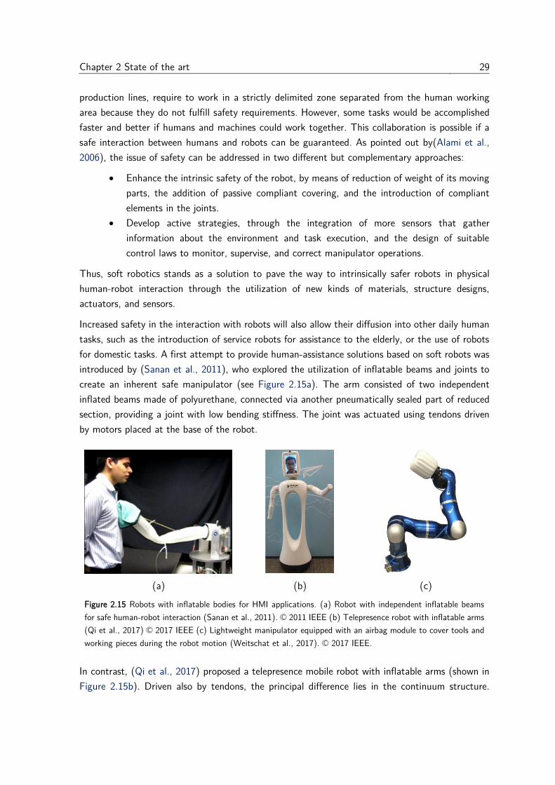
Chapter 2 State of the art 29

production lines, require to work in a strictly delimited zone separated from the human working

area because they do not fulfill safety requirements. However, some tasks would be accomplished

faster and better if humans and machines could work together. This collaboration is possible if a

safe interaction between humans and robots can be guaranteed. As pointed out by(Alami et al.,

2006), the issue of safety can be addressed in two different but complementary approaches:

• Enhance the intrinsic safety of the robot, by means of reduction of weight of its moving

parts, the addition of passive compliant covering, and the introduction of compliant

elements in the joints.

• Develop active strategies, through the integration of more sensors that gather

information about the environment and task execution, and the design of suitable

control laws to monitor, supervise, and correct manipulator operations.

Thus, soft robotics stands as a solution to pave the way to intrinsically safer robots in physical

human-robot interaction through the utilization of new kinds of materials, structure designs,

actuators, and sensors.

Increased safety in the interaction with robots will also allow their diffusion into other daily human

tasks, such as the introduction of service robots for assistance to the elderly, or the use of robots

for domestic tasks. A first attempt to provide human-assistance solutions based on soft robots was

introduced by (Sanan et al., 2011), who explored the utilization of inflatable beams and joints to

create an inherent safe manipulator (see Figure 2.15a). The arm consisted of two independent

inflated beams made of polyurethane, connected via another pneumatically sealed part of reduced

section, providing a joint with low bending stiffness. The joint was actuated using tendons driven

by motors placed at the base of the robot.

(a) (b) (c)

Figure 2.15 Robots with inflatable bodies for HMI applications. (a) Robot with independent inflatable beams

for safe human-robot interaction (Sanan et al., 2011). © 2011 IEEE (b) Telepresence robot with inflatable arms

(Qi et al., 2017) © 2017 IEEE (c) Lightweight manipulator equipped with an airbag module to cover tools and

working pieces during the robot motion (Weitschat et al., 2017). © 2017 IEEE.

In contrast, (Qi et al., 2017) proposed a telepresence mobile robot with inflatable arms (shown in

Figure 2.15b). Driven also by tendons, the principal difference lies in the continuum structure.

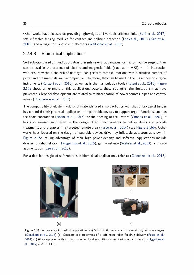
30 2.2 Soft robotics

Other works have focused on providing lightweight and variable stiffness links (Stilli et al., 2017),

soft inflatable sensing modules for contact and collision detection (Lee et al., 2013) (Kim et al.,

2018), and airbags for robotic end effectors (Weitschat et al., 2017).

2.2.4.3 Biomedical applications

Soft robotics based on fluidic actuators presents several advantages for micro-invasive surgery: they

can be used in the presence of electric and magnetic fields (such as in MRI), run in interaction

with tissues without the risk of damage, can perform complex motions with a reduced number of

parts, and the materials are biocompatible. Therefore, they can be used in the main body of surgical

instruments (Ranzani et al., 2015), as well as in the manipulation tools (Rateni et al., 2015). Figure

2.16a shows an example of this application. Despite these strengths, the limitations that have

prevented a broader development are related to miniaturization of power sources, pipes and control

valves (Polygerinos et al., 2017).

The compatibility of elastic modulus of materials used in soft robotics with that of biological tissues

has extended their potential application in implantable devices to support organ functions, such as

the heart contraction (Roche et al., 2017), or the opening of the urethra (Chonan et al., 1997). It

has also aroused an interest in the design of soft micro-robots to deliver drugs and provide

treatments and therapies in a targeted remote area (Fusco et al., 2014) (see Figure 2.16b). Other

works have focused on the design of wearable devices driven by inflatable actuators as shown in

Figure 2.16c, taking advantage of their high power density and softness. Applications include

devices for rehabilitation (Polygerinos et al., 2015), gait assistance (Wehner et al., 2013), and force

augmentation (Lee et al., 2018).

For a detailed insight of soft robotics in biomedical applications, refer to (Cianchetti et al., 2018).

(b)

(a) (c)

Figure 2.16 Soft robotics in medical applications. (a) Soft robotic manipulator for minimally invasive surgery

(Cianchetti et al., 2018) (b) Concepts and prototypes of a soft micro-robot for drug delivery (Fusco et al.,

2014) (c) Glove equipped with soft actuators for hand rehabilitation and task-specific training (Polygerinos et

al., 2015) © 2015 IEEE.

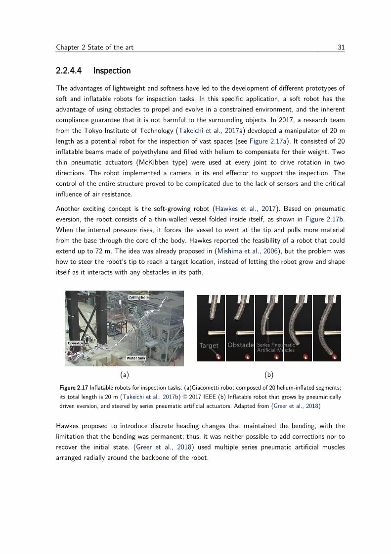
Chapter 2 State of the art 31

2.2.4.4 Inspection

The advantages of lightweight and softness have led to the development of different prototypes of

soft and inflatable robots for inspection tasks. In this specific application, a soft robot has the

advantage of using obstacles to propel and evolve in a constrained environment, and the inherent

compliance guarantee that it is not harmful to the surrounding objects. In 2017, a research team

from the Tokyo Institute of Technology (Takeichi et al., 2017a) developed a manipulator of 20 m

length as a potential robot for the inspection of vast spaces (see Figure 2.17a). It consisted of 20

inflatable beams made of polyethylene and filled with helium to compensate for their weight. Two

thin pneumatic actuators (McKibben type) were used at every joint to drive rotation in two

directions. The robot implemented a camera in its end effector to support the inspection. The

control of the entire structure proved to be complicated due to the lack of sensors and the critical

influence of air resistance.

Another exciting concept is the soft-growing robot (Hawkes et al., 2017). Based on pneumatic

eversion, the robot consists of a thin-walled vessel folded inside itself, as shown in Figure 2.17b.

When the internal pressure rises, it forces the vessel to evert at the tip and pulls more material

from the base through the core of the body. Hawkes reported the feasibility of a robot that could

extend up to 72 m. The idea was already proposed in (Mishima et al., 2006), but the problem was

how to steer the robot's tip to reach a target location, instead of letting the robot grow and shape

itself as it interacts with any obstacles in its path.

(a) (b)

Figure 2.17 Inflatable robots for inspection tasks. (a)Giacometti robot composed of 20 helium-inflated segments;

its total length is 20 m (Takeichi et al., 2017b) © 2017 IEEE (b) Inflatable robot that grows by pneumatically

driven eversion, and steered by series pneumatic artificial actuators. Adapted from (Greer et al., 2018)

Hawkes proposed to introduce discrete heading changes that maintained the bending, with the

limitation that the bending was permanent; thus, it was neither possible to add corrections nor to

recover the initial state. (Greer et al., 2018) used multiple series pneumatic artificial muscles

arranged radially around the backbone of the robot.

Series PneumaticArti cial Muscles

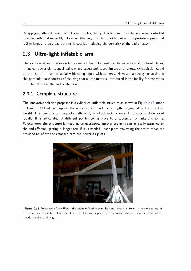
32 2.3 Ultra-light inflatable arm

By applying different pressures to those muscles, the tip direction and the extension were controlled

independently and reversibly. However, the length of the robot is limited, the prototype presented

is 2 m long, and only one bending is possible, reducing the dexterity of the end effector.

2.3 Ultra-light inflatable arm

The solution of an inflatable robot came out from the need for the inspection of confined places,

in nuclear power plants specifically, where access points are limited and narrow. One solution could

be the use of unmanned aerial vehicles equipped with cameras. However, a strong constraint in

this particular case consists of assuring that all the material introduced in the facility for inspection

must be retired at the end of the task.

2.3.1 Complete structure

The innovative solution proposed is a cylindrical inflatable structure as shown in Figure 2.18, made

of Dyneema® that can support the inner pressure and the strengths originated by the structure

weight. The structure can be packed efficiently in a backpack for ease of transport and deployed

rapidly. It is articulated at different points, giving place to a succession of links and joints.

Furthermore, the structure is modular, using zippers, another segment can be easily attached to

the end effector, getting a longer arm if it is needed. Inner pipes traversing the entire robot are

provided to inflate the attached arm and power its joints.

Figure 2.18 Prototype of the Ultra-lightweight inflatable arm. Its total length is 10 m, it has 6 degrees of

freedom, a cross-section diameter of 30 cm. The last segment with a smaller diameter can be detached to

modulate the total length.

Chapter 2 State of the art 33

2.3.2 Joint

Every joint has a rotation range of 180° approximately. It is constructed using two symmetric and

inextensible bands that maintain two consecutive cylindrical links close one to the other (refer to

Figure 2.19). This approach differs from a previous concept (Voisembert et al., 2013) that proposed

a joint with constant volume that changes its geometry from a straight cylinder to a quarter of

torus. The utilization of inextensible bands brings closer both links, reducing the dislocation problem

that appears under loading. Furthermore, as the length of the joint is reduced, the rotation

concentrates around a single axis, which simplifies the geometric and kinematic model of the entire

structure enormously.

Figure 2.19 Architecture of the long-range inflatable robot. Every joint is driven by two inflatable actuators put

in an antagonistic setup to turn in both directions.

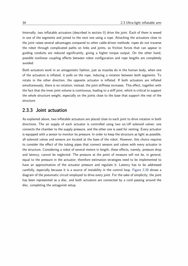
34 2.3 Ultra-light inflatable arm

Internally, two inflatable actuators (described in section 0) drive the joint. Each of them is sewed

in one of the segments and joined to the next one using a rope. Attaching the actuators close to

the joint raises several advantages compared to other cable-driven methods: ropes do not traverse

the robot through complicated paths on links and joints, so friction forces that can appear in

guiding conduits are reduced significantly, giving a higher torque output. On the other hand,

possible nonlinear coupling effects between robot configuration and rope lengths are completely

avoided.

Both actuators work in an antagonistic fashion, just as muscles do in the human body, when one

of the actuators is inflated, it pulls on the rope, inducing a rotation between both segments. To

rotate in the other direction, the opposite actuator is inflated. If both actuators are inflated

simultaneously, there is no rotation; instead, the joint stiffness increases. This effect, together with

the fact that the inner joint volume is continuous, leading to a stiff joint, which is critical to support

the whole structure weight, especially on the joints close to the base that support the rest of the

structure.

2.3.3 Joint actuation

As explained above, two inflatable actuators are placed close to each joint to drive rotation in both

directions. The air supply of each actuator is controlled using two on/off solenoid valves: one

connects the chamber to the supply pressure, and the other one is used for venting. Every actuator

is equipped with a sensor to monitor its pressure. In order to keep the structure as light as possible,

all solenoid valves and sensors are located at the base of the robot. However, this choice requires

to consider the effect of the tubing pipes that connect sensors and valves with every actuator in

the structure. Considering a robot of several meters in length, these effects, namely, pressure drop

and latency, cannot be neglected. The pressure at the point of measure will not be, in general,

equal to the pressure in the actuator; therefore estimation strategies need to be implemented to

have an approximation of the actuator pressure and regulate it. Latency has to be addressed

carefully, especially because it is a source of instability in the control loop. Figure 2.20 shows a

diagram of the pneumatic circuit employed to drive every joint. For the sake of simplicity, the joint

has been represented as a disc, and both actuators are connected by a cord passing around the

disc, completing the antagonist setup.

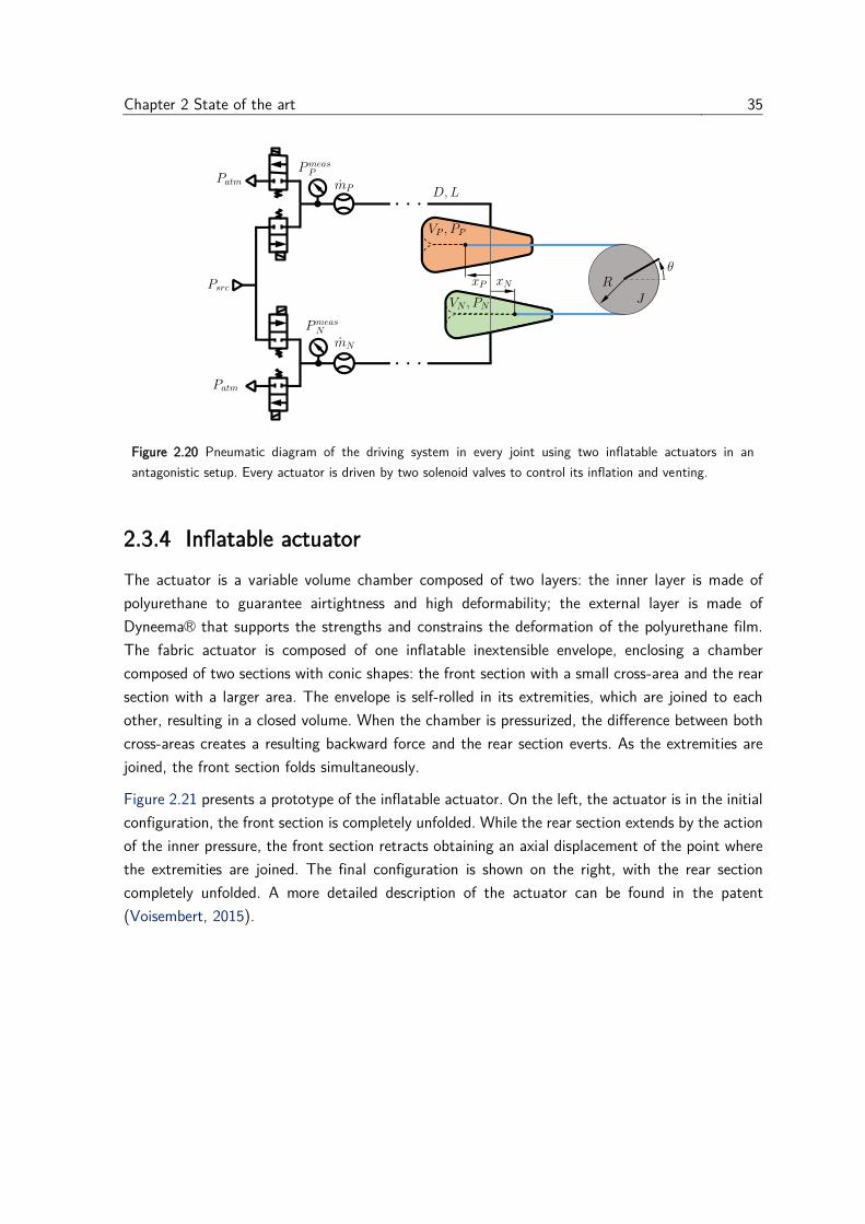
Chapter 2 State of the art 35

Figure 2.20 Pneumatic diagram of the driving system in every joint using two inflatable actuators in an

antagonistic setup. Every actuator is driven by two solenoid valves to control its inflation and venting.

2.3.4 Inflatable actuator

The actuator is a variable volume chamber composed of two layers: the inner layer is made of

polyurethane to guarantee airtightness and high deformability; the external layer is made of

Dyneema® that supports the strengths and constrains the deformation of the polyurethane film.

The fabric actuator is composed of one inflatable inextensible envelope, enclosing a chamber

composed of two sections with conic shapes: the front section with a small cross-area and the rear

section with a larger area. The envelope is self-rolled in its extremities, which are joined to each

other, resulting in a closed volume. When the chamber is pressurized, the difference between both

cross-areas creates a resulting backward force and the rear section everts. As the extremities are

joined, the front section folds simultaneously.

Figure 2.21 presents a prototype of the inflatable actuator. On the left, the actuator is in the initial

configuration, the front section is completely unfolded. While the rear section extends by the action

of the inner pressure, the front section retracts obtaining an axial displacement of the point where

the extremities are joined. The final configuration is shown on the right, with the rear section

completely unfolded. A more detailed description of the actuator can be found in the patent

(Voisembert, 2015).

36 2.4 Conclusions

Figure 2.21 Prototype of the inflatable actuator in three different configurations.

2.4 Conclusions

Inflatable structures have evolved quickly in the last century. This development has been motivated

by four simple but powerful features: inflatable structures are lightweight, they can be packed

efficiently, they are easy to deploy, and they are soft. Thus, these kinds of structures have found

numerous applications, from shelters, greenhouses, and nomad platforms to lightweight means of

transport, and is a promising solution for future spatial missions and habitats on other planets.

The development of this field has also benefited from advances in synthesis, characterization, and

production of lighter and more resistant materials.

On the other hand, soft robotics is a field in a rapid expansion that aims to design, model, create,

and control robots made of compliant materials. These robots are not as precise as their rigid

counterparts; instead, they are versatile, adapting quickly to a variety of situations and tasks where

conventional robots still fail. Soft robotics is opening new horizons in a wide range of fields, such

as human-robot interaction, delicate manipulation, minimally invasive surgery, or inspection of

confined and hazardous environments.

The advancement of soft robotics lies on different research axes: development of more effective

materials, new kinds of lightweight and reliable actuators, sensors adapted to deformable structures,

as well as modeling and control of continuum deformable bodies. Coming chapters intend to

contribute in the study of new lightweight actuators, sensors and control strategies, adapted for a

long-range inflatable manipulator whose first application is the inspection of confined environments,

but not restricted to it. On the other hand, soft robotics is a field in a rapid expansion that aims

to design, model, create, and control robots made of compliant materials. These robots are not as

precise as their rigid counterparts; instead, they are versatile, adapting quickly to a variety of

situations and tasks where conventional robots still fail. Soft robotics is opening new horizons in a

wide range of fields, such as human-robot interaction, delicate manipulation, minimally invasive

surgery, or inspection in confined and hazardous environments.

Chapter 3

Inflatable actuator

Our nature consists in motion; complete rest is

death

― Blaise Pascal

Contents

3.1 State of the art ................................................................................................ 38

3.1.1 Expansion ................................................................................................... 38

3.1.2 Contraction ................................................................................................ 39

3.1.3 Bending ...................................................................................................... 41

3.1.4 Other types ................................................................................................ 42

3.2 Actuator description.......................................................................................... 43

3.3 Cylindrical actuator ........................................................................................... 44

3.3.1 Analytical model ......................................................................................... 44

3.3.2 Experimental characterization ..................................................................... 48

3.3.3 Instability ................................................................................................... 49

3.4 Conical actuator ............................................................................................... 51

3.4.1 Analytical model ......................................................................................... 51

3.4.2 Experimental Characterization ..................................................................... 55

3.4.3 Finite elements analysis ............................................................................... 58

3.5 Conclusions ...................................................................................................... 66

This chapter presents, first, a state of the art of actuators for soft robotics. Then, the concept of

the inflatable actuator employed in the long-range inflatable arm is described, and two different

geometries (cylindrical and conical) are analyzed in detail, establishing analytical models of the

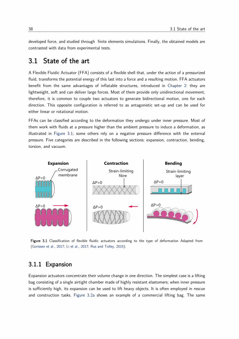
38 3.1 State of the art

developed force, and studied through finite elements simulations. Finally, the obtained models are

contrasted with data from experimental tests.

3.1 State of the art

A Flexible Fluidic Actuator (FFA) consists of a flexible shell that, under the action of a pressurized

fluid, transforms the potential energy of this last into a force and a resulting motion. FFA actuators

benefit from the same advantages of inflatable structures, introduced in Chapter 2: they are

lightweight, soft and can deliver large forces. Most of them provide only unidirectional movement,

therefore, it is common to couple two actuators to generate bidirectional motion, one for each

direction. This opposite configuration is referred to as antagonistic set-up and can be used for

either linear or rotational motion.

FFAs can be classified according to the deformation they undergo under inner pressure. Most of

them work with fluids at a pressure higher than the ambient pressure to induce a deformation, as

illustrated in Figure 3.1; some others rely on a negative pressure difference with the external

pressure. Five categories are described in the following sections: expansion, contraction, bending,

torsion, and vacuum.

Figure 3.1 Classification of flexible fluidic actuators according to the type of deformation Adapted from

(Gorissen et al., 2017; Li et al., 2017; Rus and Tolley, 2015).

3.1.1 Expansion

Expansion actuators concentrate their volume change in one direction. The simplest case is a lifting

bag consisting of a single airtight chamber made of highly resistant elastomers; when inner pressure

is sufficiently high, its expansion can be used to lift heavy objects. It is often employed in rescue

and construction tasks. Figure 3.2a shows an example of a commercial lifting bag. The same

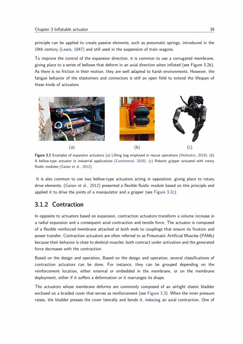
Chapter 3 Inflatable actuator 39

principle can be applied to create passive elements, such as pneumatic springs, introduced in the

19th century (Lewis, 1847) and still used in the suspension of train wagons.

To improve the control of the expansion direction, it is common to use a corrugated membrane,

giving place to a series of bellows that deform in an axial direction when inflated (see Figure 3.2b).

As there is no friction in their motion, they are well adapted to harsh environments. However, the

fatigue behavior of the elastomers and connectors is still an open field to extend the lifespan of

these kinds of actuators.

(a) (b) (c)

Figure 3.2 Examples of expansion actuators (a) Lifting bag employed in rescue operations (Holmatro, 2019). (b)

A bellow-type actuator in industrial applications (Continental, 2019). (c) Robotic gripper actuated with rotary

fluidic modules (Gaiser et al., 2012).

It is also common to use two bellow-type actuators acting in opposition, giving place to rotary

drive elements. (Gaiser et al., 2012) presented a flexible fluidic module based on this principle and

applied it to drive the joints of a manipulator and a gripper (see Figure 3.2c).

3.1.2 Contraction

In opposite to actuators based on expansion, contraction actuators transform a volume increase in

a radial expansion and a consequent axial contraction and tensile force. The actuator is composed

of a flexible reinforced membrane attached at both ends to couplings that ensure its fixation and

power transfer. Contraction actuators are often referred to as Pneumatic Artificial Muscles (PAMs)

because their behavior is close to skeletal muscles: both contract under activation and the generated

force decreases with the contraction.

Based on the design and operation, Based on the design and operation, several classifications of

contraction actuators can be done. For instance, they can be grouped depending on the

reinforcement location, either external or embedded in the membrane, or on the membrane

deployment, either if it suffers a deformation or it rearranges its shape.

The actuators whose membrane deforms are commonly composed of an airtight elastic bladder

enclosed on a braided cover that serves as reinforcement (see Figure 3.3). When the inner pressure

raises, the bladder presses the cover laterally and bends it, inducing an axial contraction. One of

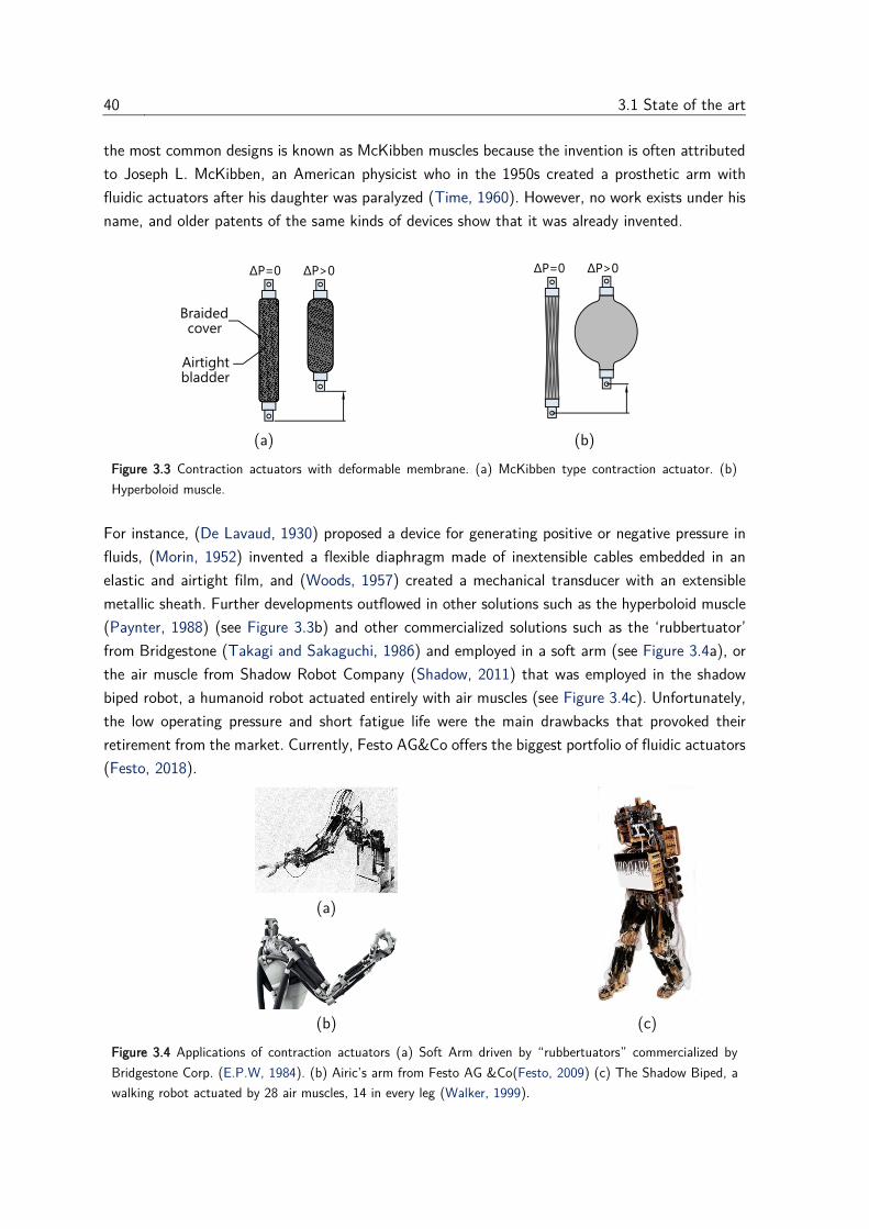
40 3.1 State of the art

the most common designs is known as McKibben muscles because the invention is often attributed

to Joseph L. McKibben, an American physicist who in the 1950s created a prosthetic arm with

fluidic actuators after his daughter was paralyzed (Time, 1960). However, no work exists under his

name, and older patents of the same kinds of devices show that it was already invented.

(a) (b)

Figure 3.3 Contraction actuators with deformable membrane. (a) McKibben type contraction actuator. (b)

Hyperboloid muscle.

For instance, (De Lavaud, 1930) proposed a device for generating positive or negative pressure in

fluids, (Morin, 1952) invented a flexible diaphragm made of inextensible cables embedded in an

elastic and airtight film, and (Woods, 1957) created a mechanical transducer with an extensible

metallic sheath. Further developments outflowed in other solutions such as the hyperboloid muscle

(Paynter, 1988) (see Figure 3.3b) and other commercialized solutions such as the ‘rubbertuator’

from Bridgestone (Takagi and Sakaguchi, 1986) and employed in a soft arm (see Figure 3.4a), or

the air muscle from Shadow Robot Company (Shadow, 2011) that was employed in the shadow

biped robot, a humanoid robot actuated entirely with air muscles (see Figure 3.4c). Unfortunately,

the low operating pressure and short fatigue life were the main drawbacks that provoked their

retirement from the market. Currently, Festo AG&Co offers the biggest portfolio of fluidic actuators

(Festo, 2018).

(a)

(b) (c)

Figure 3.4 Applications of contraction actuators (a) Soft Arm driven by “rubbertuators” commercialized by

Bridgestone Corp. (E.P.W, 1984). (b) Airic’s arm from Festo AG &Co(Festo, 2009) (c) The Shadow Biped, a

walking robot actuated by 28 air muscles, 14 in every leg (Walker, 1999).

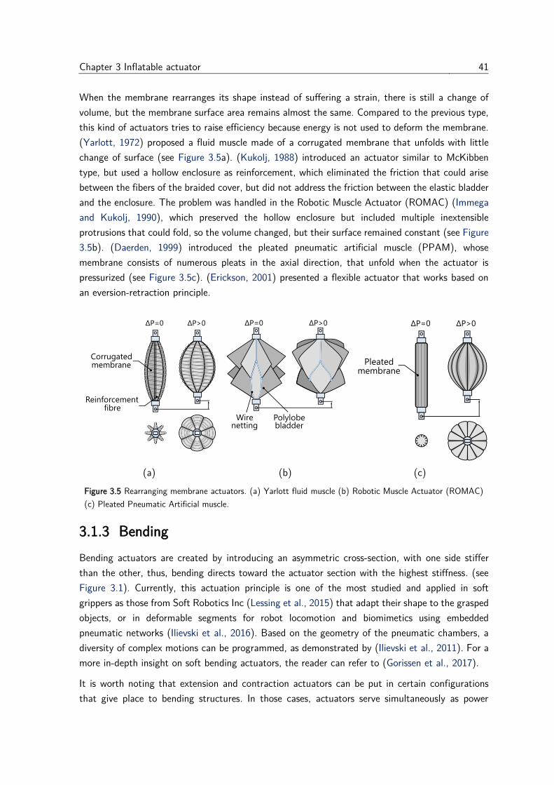
Chapter 3 Inflatable actuator 41

When the membrane rearranges its shape instead of suffering a strain, there is still a change of

volume, but the membrane surface area remains almost the same. Compared to the previous type,

this kind of actuators tries to raise efficiency because energy is not used to deform the membrane.

(Yarlott, 1972) proposed a fluid muscle made of a corrugated membrane that unfolds with little

change of surface (see Figure 3.5a). (Kukolj, 1988) introduced an actuator similar to McKibben

type, but used a hollow enclosure as reinforcement, which eliminated the friction that could arise

between the fibers of the braided cover, but did not address the friction between the elastic bladder

and the enclosure. The problem was handled in the Robotic Muscle Actuator (ROMAC) (Immega

and Kukolj, 1990), which preserved the hollow enclosure but included multiple inextensible

protrusions that could fold, so the volume changed, but their surface remained constant (see Figure

3.5b). (Daerden, 1999) introduced the pleated pneumatic artificial muscle (PPAM), whose

membrane consists of numerous pleats in the axial direction, that unfold when the actuator is

pressurized (see Figure 3.5c). (Erickson, 2001) presented a flexible actuator that works based on

an eversion-retraction principle.

(a) (b) (c)

Figure 3.5 Rearranging membrane actuators. (a) Yarlott fluid muscle (b) Robotic Muscle Actuator (ROMAC)

(c) Pleated Pneumatic Artificial muscle.

3.1.3 Bending

Bending actuators are created by introducing an asymmetric cross-section, with one side stiffer

than the other, thus, bending directs toward the actuator section with the highest stiffness. (see

Figure 3.1). Currently, this actuation principle is one of the most studied and applied in soft

grippers as those from Soft Robotics Inc (Lessing et al., 2015) that adapt their shape to the grasped

objects, or in deformable segments for robot locomotion and biomimetics using embedded

pneumatic networks (Ilievski et al., 2016). Based on the geometry of the pneumatic chambers, a

diversity of complex motions can be programmed, as demonstrated by (Ilievski et al., 2011). For a

more in-depth insight on soft bending actuators, the reader can refer to (Gorissen et al., 2017).

It is worth noting that extension and contraction actuators can be put in certain configurations

that give place to bending structures. In those cases, actuators serve simultaneously as power

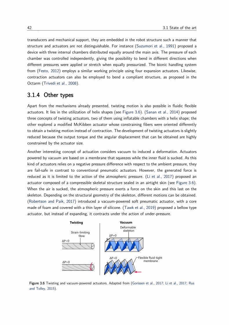
42 3.1 State of the art

transducers and mechanical support, they are embedded in the robot structure such a manner that

structure and actuators are not distinguishable. For instance (Suzumori et al., 1991) proposed a

device with three internal chambers distributed equally around the main axis. The pressure of each

chamber was controlled independently, giving the possibility to bend in different directions when

different pressures were applied or stretch when equally pressurized. The bionic handling system

from (Festo, 2012) employs a similar working principle using four expansion actuators. Likewise,

contraction actuators can also be employed to bend a compliant structure, as proposed in the

Octarm (Trivedi et al., 2008).

3.1.4 Other types

Apart from the mechanisms already presented, twisting motion is also possible in fluidic flexible

actuators. It lies in the utilization of helix shapes (see Figure 3.6). (Sanan et al., 2014) proposed

three concepts of twisting actuators, two of them using inflatable chambers with a helix shape; the

other explored a modified McKibben actuator whose constraining fibers were oriented differently

to obtain a twisting motion instead of contraction. The development of twisting actuators is slightly

reduced because the output torque and the angular displacement that can be obtained are highly

constrained by the actuator size.

Another interesting concept of actuation considers vacuum to induced a deformation. Actuators

powered by vacuum are based on a membrane that squeezes while the inner fluid is sucked. As this

kind of actuators relies on a negative pressure difference with respect to the ambient pressure, they

are fail-safe in contrast to conventional pneumatic actuators. However, the generated force is

reduced as it is limited to the action of the atmospheric pressure. (Li et al., 2017) proposed an

actuator composed of a compressible skeletal structure sealed in an airtight skin (see Figure 3.6).

When the air is sucked, the atmospheric pressure exerts a force on the skin and this last on the

skeleton. Depending on the structural geometry of the skeleton, different motions can be obtained.

(Robertson and Paik, 2017) introduced a vacuum-powered soft pneumatic actuator, with a core

made of foam and covered with a thin layer of silicone. (Tawk et al., 2019) proposed a bellow type

actuator, but instead of expanding, it contracts under the action of under-pressure.

Figure 3.6 Twisting and vacuum-powered actuators. Adapted from (Gorissen et al., 2017; Li et al., 2017; Rus

and Tolley, 2015).

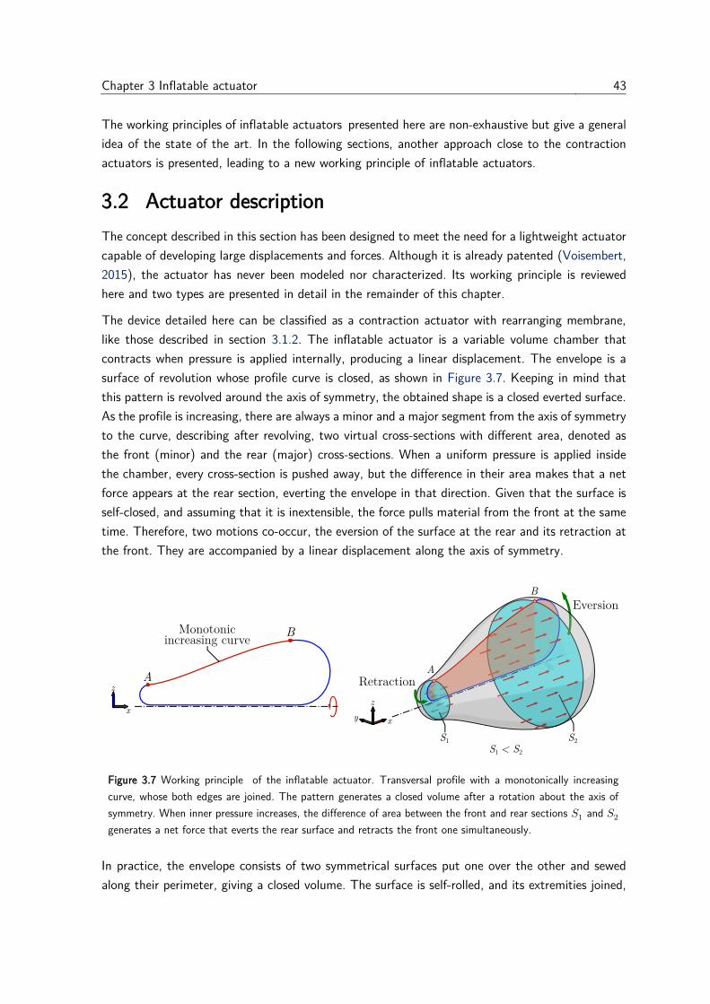
Chapter 3 Inflatable actuator 43

The working principles of inflatable actuators presented here are non-exhaustive but give a general

idea of the state of the art. In the following sections, another approach close to the contraction

actuators is presented, leading to a new working principle of inflatable actuators.

3.2 Actuator description

The concept described in this section has been designed to meet the need for a lightweight actuator

capable of developing large displacements and forces. Although it is already patented (Voisembert,

2015), the actuator has never been modeled nor characterized. Its working principle is reviewed

here and two types are presented in detail in the remainder of this chapter.

The device detailed here can be classified as a contraction actuator with rearranging membrane,

like those described in section 3.1.2. The inflatable actuator is a variable volume chamber that

contracts when pressure is applied internally, producing a linear displacement. The envelope is a

surface of revolution whose profile curve is closed, as shown in Figure 3.7. Keeping in mind that

this pattern is revolved around the axis of symmetry, the obtained shape is a closed everted surface.

As the profile is increasing, there are always a minor and a major segment from the axis of symmetry

to the curve, describing after revolving, two virtual cross-sections with different area, denoted as

the front (minor) and the rear (major) cross-sections. When a uniform pressure is applied inside

the chamber, every cross-section is pushed away, but the difference in their area makes that a net

force appears at the rear section, everting the envelope in that direction. Given that the surface is

self-closed, and assuming that it is inextensible, the force pulls material from the front at the same

time. Therefore, two motions co-occur, the eversion of the surface at the rear and its retraction at

the front. They are accompanied by a linear displacement along the axis of symmetry.

Figure 3.7 Working principle of the inflatable actuator. Transversal profile with a monotonically increasing

curve, whose both edges are joined. The pattern generates a closed volume after a rotation about the axis of

symmetry. When inner pressure increases, the difference of area between the front and rear sections 𝑆1 and 𝑆2

generates a net force that everts the rear surface and retracts the front one simultaneously.

In practice, the envelope consists of two symmetrical surfaces put one over the other and sewed

along their perimeter, giving a closed volume. The surface is self-rolled, and its extremities joined,

44 3.3 Cylindrical actuator

where a string is also sewed that will transfer the force and displacement. The membrane is made

of two layers: A film of polyurethane makes the chamber airtight, while a woven fiber shell made

of Dyneema® constrains the deformation and supports the strengths.

Depending on the shape of the surface, different geometries can be obtained. The rest of this

chapter focus on the study of two cases: cylindrical and conic shapes.

3.3 Cylindrical actuator

In this case, the front and rear sections are cylinders that have different radii to keep a constant

difference of cross-areas that creates the pulling force. Figure 3.8 presents a 3D representation of

the actuator. On the left, the actuator is in the initial configuration, the front section, colored in

red, is wholly everted. While the rear section everts by the action of the resultant force, the front

section retracts obtaining an axial displacement of the point where the extremities are joined. The

final configuration is shown on the right, the rear section colored in blue is completely everted.

Figure 3.8 3D representation of the cylindrical actuator in its initial and final configurations. The green surface

stays fixed, while the blue and red surfaces can evert and retract to obtain a linear displacement.

3.3.1 Analytical model

In a standard pneumatic cylinder, the expressions relating volume, inner pressure, force, and tip

position are well known. For an inflatable chamber such as that shown in Figure 3.8, the following

question arises: can we obtain similar expressions that will be helpful for modeling and simulation

of the driving setup? This section develops a geometric study to find relations between the volume

and the tip displacement, as well as static analysis to get a relationship between the transferred

force, the tip position, and internal pressure. For that, the following assumptions are made:

• The chamber is axisymmetric for any tip displacement. Thus, the analysis of the

transversal section is enough to describe the behavior of the entire volume.

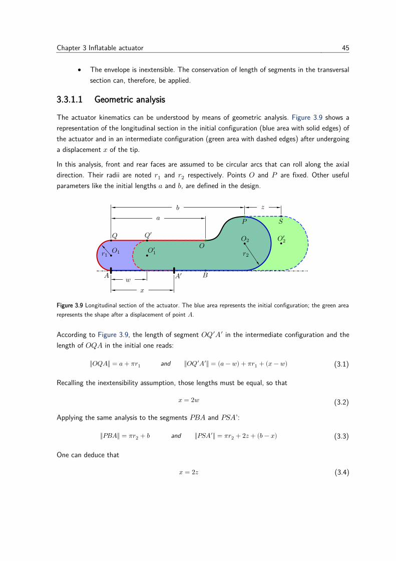
Chapter 3 Inflatable actuator 45

• The envelope is inextensible. The conservation of length of segments in the transversal

section can, therefore, be applied.

3.3.1.1 Geometric analysis

The actuator kinematics can be understood by means of geometric analysis. Figure 3.9 shows a

representation of the longitudinal section in the initial configuration (blue area with solid edges) of

the actuator and in an intermediate configuration (green area with dashed edges) after undergoing

a displacement 𝑥 of the tip.

In this analysis, front and rear faces are assumed to be circular arcs that can roll along the axial

direction. Their radii are noted 𝑟1 and 𝑟2 respectively. Points 𝑂 and 𝑃 are fixed. Other useful

parameters like the initial lengths 𝑎 and 𝑏, are defined in the design.

Figure 3.9 Longitudinal section of the actuator. The blue area represents the initial configuration; the green area

represents the shape after a displacement of point 𝐴.

According to Figure 3.9, the length of segment 𝑂𝑄′𝐴′ in the intermediate configuration and the

length of 𝑂𝑄𝐴 in the initial one reads:

‖𝑂𝑄𝐴‖ = 𝑎 + 𝜋𝑟1 and ‖𝑂𝑄′𝐴′‖ = (𝑎 − 𝑤) + 𝜋𝑟1 + (𝑥 − 𝑤) (3.1)

Recalling the inextensibility assumption, those lengths must be equal, so that

𝑥 = 2𝑤 (3.2)

Applying the same analysis to the segments 𝑃𝐵𝐴 and 𝑃𝑆𝐴’:

‖𝑃𝐵𝐴‖ = 𝜋𝑟2 + 𝑏 and ‖𝑃𝑆𝐴′‖ = 𝜋𝑟2 + 2𝑧 + (𝑏 − 𝑥) (3.3)

One can deduce that

𝑥 = 2𝑧 (3.4)

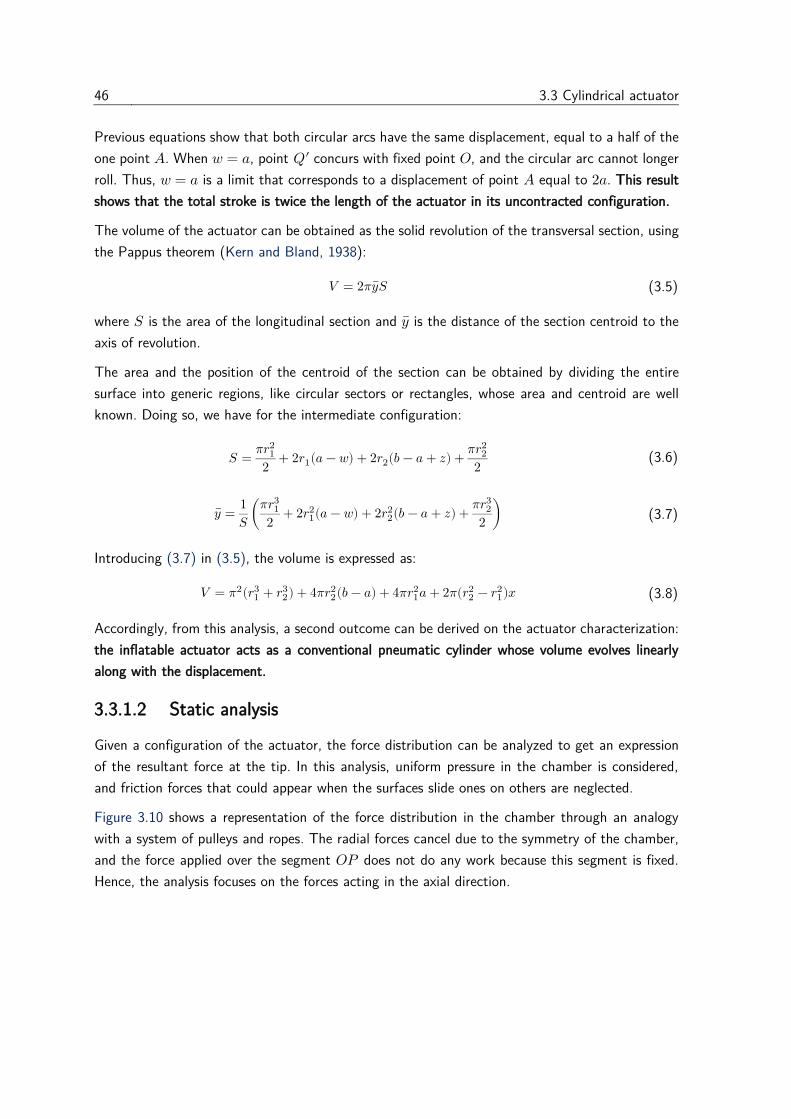
46 3.3 Cylindrical actuator

Previous equations show that both circular arcs have the same displacement, equal to a half of the

one point 𝐴. When 𝑤 = 𝑎, point 𝑄′ concurs with fixed point 𝑂, and the circular arc cannot longer

roll. Thus, 𝑤 = 𝑎 is a limit that corresponds to a displacement of point 𝐴 equal to 2𝑎. This result

shows that the total stroke is twice the length of the actuator in its uncontracted configuration.

The volume of the actuator can be obtained as the solid revolution of the transversal section, using

the Pappus theorem (Kern and Bland, 1938):

𝑉 = 2𝜋𝑦�̅� (3.5)

where 𝑆 is the area of the longitudinal section and 𝑦 ̅is the distance of the section centroid to the

axis of revolution.

The area and the position of the centroid of the section can be obtained by dividing the entire

surface into generic regions, like circular sectors or rectangles, whose area and centroid are well

known. Doing so, we have for the intermediate configuration:

𝑆 =𝜋𝑟12

2+ 2𝑟1(𝑎 − 𝑤) + 2𝑟2(𝑏 − 𝑎 + 𝑧) +

𝜋𝑟22

2 (3.6)

𝑦 ̅ =1

𝑆(𝜋𝑟13

2+ 2𝑟1

2(𝑎 − 𝑤) + 2𝑟22(𝑏 − 𝑎 + 𝑧) +

𝜋𝑟23

2) (3.7)

Introducing (3.7) in (3.5), the volume is expressed as:

𝑉 = 𝜋2(𝑟13 + 𝑟2

3) + 4𝜋𝑟22(𝑏 − 𝑎) + 4𝜋𝑟1

2𝑎 + 2𝜋(𝑟22 − 𝑟1

2)𝑥 (3.8)

Accordingly, from this analysis, a second outcome can be derived on the actuator characterization:

the inflatable actuator acts as a conventional pneumatic cylinder whose volume evolves linearly

along with the displacement.

3.3.1.2 Static analysis

Given a configuration of the actuator, the force distribution can be analyzed to get an expression

of the resultant force at the tip. In this analysis, uniform pressure in the chamber is considered,

and friction forces that could appear when the surfaces slide ones on others are neglected.

Figure 3.10 shows a representation of the force distribution in the chamber through an analogy

with a system of pulleys and ropes. The radial forces cancel due to the symmetry of the chamber,

and the force applied over the segment 𝑂𝑃 does not do any work because this segment is fixed.

Hence, the analysis focuses on the forces acting in the axial direction.

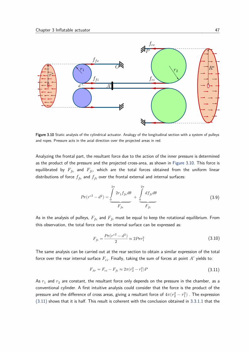
Chapter 3 Inflatable actuator 47

Figure 3.10 Static analysis of the cylindrical actuator. Analogy of the longitudinal section with a system of pulleys

and ropes. Pressure acts in the axial direction over the projected areas in red.

Analyzing the frontal part, the resultant force due to the action of the inner pressure is determined

as the product of the pressure and the projected cross-area, as shown in Figure 3.10. This force is

equilibrated by 𝐹𝑓𝑒 and 𝐹𝑓𝑖, which are the total forces obtained from the uniform linear

distributions of force 𝑓𝑓𝑒 and 𝑓𝑓𝑖 over the frontal external and internal surfaces:

𝑃𝜋(𝑟∗2 − 𝑑2) =∫ 2𝑟1𝑓𝑓𝑒𝑑𝜃

2𝜋

0⏟

𝐹𝑓𝑒

+ ∫ 𝑑𝑓𝑓𝑖𝑑𝜃

2𝜋

0⏟

𝐹𝑓𝑖

(3.9)

As in the analysis of pulleys, 𝐹𝑓𝑒 and 𝐹𝑓𝑖 must be equal to keep the rotational equilibrium. From

this observation, the total force over the internal surface can be expressed as:

𝐹𝑓𝑖 =𝑃𝜋(𝑟∗2 − 𝑑2)

2≈ 2𝑃𝜋𝑟1

2 (3.10)

The same analysis can be carried out at the rear section to obtain a similar expression of the total

force over the rear internal surface 𝐹𝑟𝑖. Finally, taking the sum of forces at point 𝐴′ yields to:

𝐹𝐴′ = 𝐹𝑟𝑖 − 𝐹𝑓𝑖 ≈ 2𝜋(𝑟22 − 𝑟1

2)𝑃 (3.11)

As 𝑟1 and 𝑟2 are constant, the resultant force only depends on the pressure in the chamber, as a

conventional cylinder. A first intuitive analysis could consider that the force is the product of the

pressure and the difference of cross areas, giving a resultant force of 4𝜋(𝑟22 − 𝑟1

2) . The expression

(3.11) shows that it is half. This result is coherent with the conclusion obtained in 3.3.1.1 that the

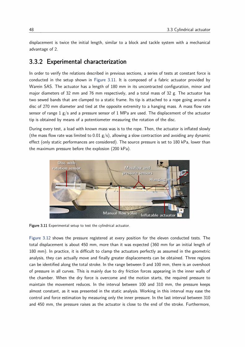
48 3.3 Cylindrical actuator

displacement is twice the initial length, similar to a block and tackle system with a mechanical

advantage of 2.

3.3.2 Experimental characterization

In order to verify the relations described in previous sections, a series of tests at constant force is

conducted in the setup shown in Figure 3.11. It is composed of a fabric actuator provided by

Warein SAS. The actuator has a length of 180 mm in its uncontracted configuration, minor and

major diameters of 32 mm and 76 mm respectively, and a total mass of 32 g. The actuator has

two sewed bands that are clamped to a static frame. Its tip is attached to a rope going around a

disc of 270 mm diameter and tied at the opposite extremity to a hanging mass. A mass flow rate

sensor of range 1 g/s and a pressure sensor of 1 MPa are used. The displacement of the actuator

tip is obtained by means of a potentiometer measuring the rotation of the disc.

During every test, a load with known mass was is to the rope. Then, the actuator is inflated slowly

(the mass flow rate was limited to 0.01 g/s), allowing a slow contraction and avoiding any dynamic

effect (only static performances are considered). The source pressure is set to 180 kPa, lower than

the maximum pressure before the explosion (200 kPa).

Figure 3.11 Experimental setup to test the cylindrical actuator.

Figure 3.12 shows the pressure registered at every position for the eleven conducted tests. The

total displacement is about 450 mm, more than it was expected (360 mm for an initial length of

180 mm). In practice, it is difficult to clamp the actuators perfectly as assumed in the geometric

analysis, they can actually move and finally greater displacements can be obtained. Three regions

can be identified along the total stroke. In the range between 0 and 100 mm, there is an overshoot

of pressure in all curves. This is mainly due to dry friction forces appearing in the inner walls of

the chamber. When the dry force is overcome and the motion starts, the required pressure to

maintain the movement reduces. In the interval between 100 and 310 mm, the pressure keeps

almost constant, as it was presented in the static analysis. Working in this interval may ease the

control and force estimation by measuring only the inner pressure. In the last interval between 310

and 450 mm, the pressure raises as the actuator is close to the end of the stroke. Furthermore,

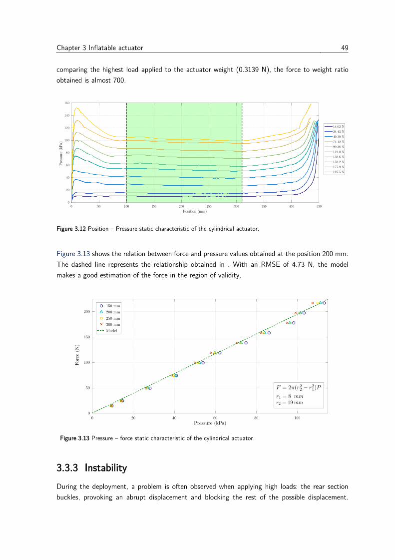
Chapter 3 Inflatable actuator 49

comparing the highest load applied to the actuator weight (0.3139 N), the force to weight ratio

obtained is almost 700.

Figure 3.12 Position – Pressure static characteristic of the cylindrical actuator.

Figure 3.13 shows the relation between force and pressure values obtained at the position 200 mm.

The dashed line represents the relationship obtained in . With an RMSE of 4.73 N, the model

makes a good estimation of the force in the region of validity.

Figure 3.13 Pressure – force static characteristic of the cylindrical actuator.

3.3.3 Instability

During the deployment, a problem is often observed when applying high loads: the rear section

buckles, provoking an abrupt displacement and blocking the rest of the possible displacement.

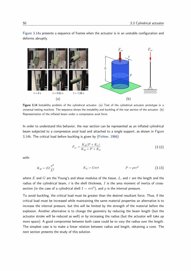
50 3.3 Cylindrical actuator

Figure 3.14a presents a sequence of frames when the actuator is in an unstable configuration and

deforms abruptly.

(a) (b)

Figure 3.14 Instability problem of the cylindrical actuator. (a) Test of the cylindrical actuator prototype in a

universal testing machine. The sequence shows the instability and buckling of the rear section of the actuator. (b)

Representation of the inflated beam under a compressive axial force.

In order to understand this behavior, the rear section can be represented as an inflated cylindrical

beam subjected to a compressive axial load and attached to a single support, as shown in Figure

3.14b. The critical load before buckling is given by (Fichter, 1966)

𝐹𝑐𝑟 =𝐾𝐵(𝑃 +𝐾𝑆)

𝐾𝐵 + 𝑃 +𝐾𝑆 (3.12)

with:

𝐾𝐵 = 𝐸𝐼𝜋2

𝐿2 𝐾𝑆 = 𝐺𝜋𝑟𝑡 𝑃 = 𝑝𝜋𝑟2 (3.13)

where 𝐸 and 𝐺 are the Young’s and shear modulus of the tissue, 𝐿, and 𝑟 are the length and the

radius of the cylindrical beam, 𝑡 is the shell thickness, 𝐼 is the area moment of inertia of cross-

section (in the case of a cylindrical shell 𝐼 = 𝜋𝑟𝑡3), and 𝑝 is the internal pressure.

To avoid buckling, the critical load must be greater than the desired resultant force. Thus, if the

critical load must be increased while maintaining the same material properties an alternative is to

increase the internal pressure, but this will be limited by the strength of the material before the

explosion. Another alternative is to change the geometry by reducing the beam length (but the

actuator stroke will be reduced as well) or by increasing the radius (but the actuator will take up

more space). A good compromise between both cases could be to vary the radius over the length.

The simplest case is to make a linear relation between radius and length, obtaining a cone. The

next section presents the study of this solution.

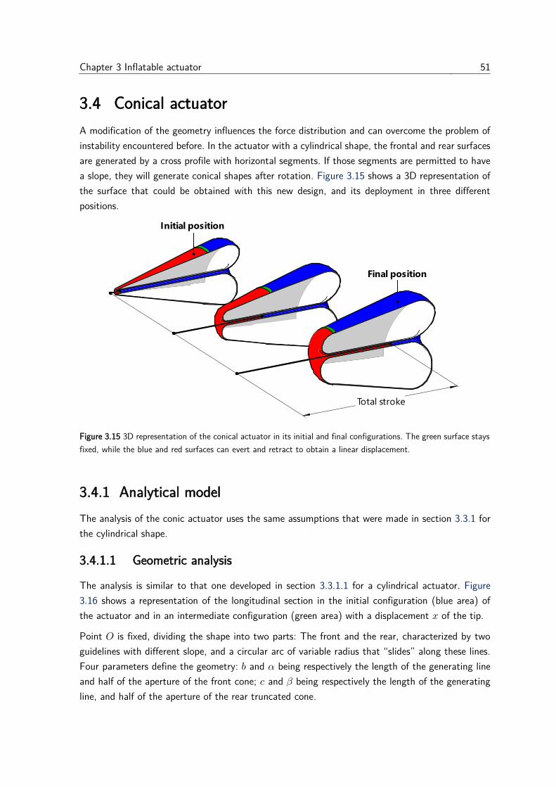
Chapter 3 Inflatable actuator 51

3.4 Conical actuator

A modification of the geometry influences the force distribution and can overcome the problem of

instability encountered before. In the actuator with a cylindrical shape, the frontal and rear surfaces

are generated by a cross profile with horizontal segments. If those segments are permitted to have

a slope, they will generate conical shapes after rotation. Figure 3.15 shows a 3D representation of

the surface that could be obtained with this new design, and its deployment in three different

positions.

Figure 3.15 3D representation of the conical actuator in its initial and final configurations. The green surface stays

fixed, while the blue and red surfaces can evert and retract to obtain a linear displacement.

3.4.1 Analytical model

The analysis of the conic actuator uses the same assumptions that were made in section 3.3.1 for

the cylindrical shape.

3.4.1.1 Geometric analysis

The analysis is similar to that one developed in section 3.3.1.1 for a cylindrical actuator. Figure

3.16 shows a representation of the longitudinal section in the initial configuration (blue area) of

the actuator and in an intermediate configuration (green area) with a displacement 𝑥 of the tip.

Point 𝑂 is fixed, dividing the shape into two parts: The front and the rear, characterized by two

guidelines with different slope, and a circular arc of variable radius that “slides” along these lines.

Four parameters define the geometry: 𝑏 and 𝛼 being respectively the length of the generating line

and half of the aperture of the front cone; 𝑐 and 𝛽 being respectively the length of the generating

line, and half of the aperture of the rear truncated cone.

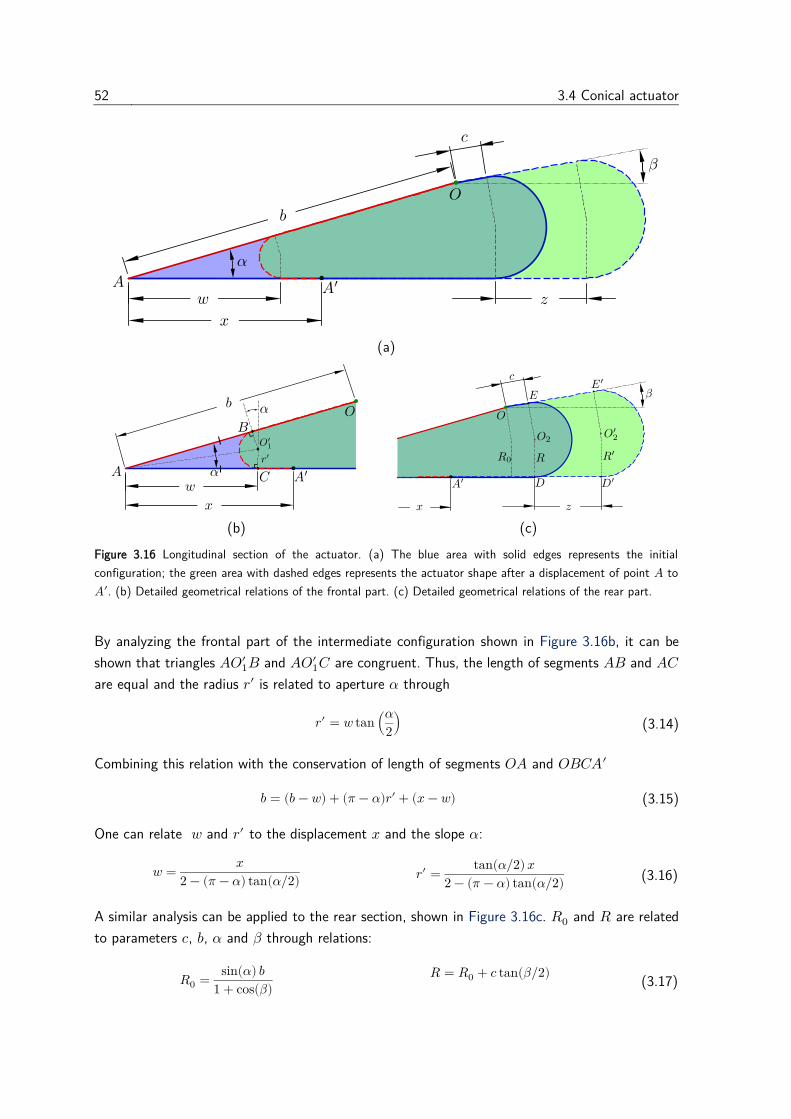
52 3.4 Conical actuator

(a)

(b) (c)

Figure 3.16 Longitudinal section of the actuator. (a) The blue area with solid edges represents the initial

configuration; the green area with dashed edges represents the actuator shape after a displacement of point 𝐴 to

𝐴′. (b) Detailed geometrical relations of the frontal part. (c) Detailed geometrical relations of the rear part.

By analyzing the frontal part of the intermediate configuration shown in Figure 3.16b, it can be

shown that triangles 𝐴𝑂1′𝐵 and 𝐴𝑂1

′𝐶 are congruent. Thus, the length of segments 𝐴𝐵 and 𝐴𝐶

are equal and the radius 𝑟′ is related to aperture 𝛼 through

𝑟′ = 𝑤 tan (𝛼

2) (3.14)

Combining this relation with the conservation of length of segments 𝑂𝐴 and 𝑂𝐵𝐶𝐴′

𝑏 = (𝑏 − 𝑤) + (𝜋 − 𝛼)𝑟′ + (𝑥 − 𝑤) (3.15)

One can relate 𝑤 and 𝑟′ to the displacement 𝑥 and the slope 𝛼:

𝑤 =𝑥

2 − (𝜋 − 𝛼) tan(𝛼 2⁄ ) 𝑟′ =

tan(𝛼 2⁄ ) 𝑥

2 − (𝜋 − 𝛼) tan(𝛼 2⁄ ) (3.16)

A similar analysis can be applied to the rear section, shown in Figure 3.16c. 𝑅0 and 𝑅 are related

to parameters 𝑐, 𝑏, 𝛼 and 𝛽 through relations:

𝑅0 =sin(𝛼) 𝑏

1 + cos(𝛽)

𝑅 = 𝑅0 + 𝑐 tan(𝛽/2) (3.17)

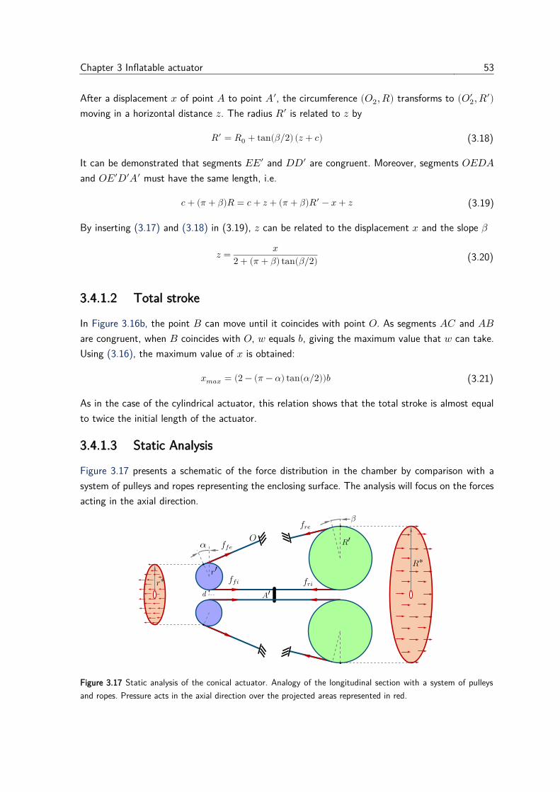
Chapter 3 Inflatable actuator 53

After a displacement 𝑥 of point 𝐴 to point 𝐴′, the circumference (𝑂2, 𝑅) transforms to (𝑂2′ , 𝑅′)

moving in a horizontal distance 𝑧. The radius 𝑅′ is related to 𝑧 by

𝑅′ = 𝑅0 + tan(𝛽/2) (𝑧 + 𝑐) (3.18)

It can be demonstrated that segments 𝐸𝐸′ and 𝐷𝐷′ are congruent. Moreover, segments 𝑂𝐸𝐷𝐴

and 𝑂𝐸′𝐷′𝐴′ must have the same length, i.e.

𝑐 + (𝜋 + 𝛽)𝑅 = 𝑐 + 𝑧 + (𝜋 + 𝛽)𝑅′ − 𝑥 + 𝑧 (3.19)

By inserting (3.17) and (3.18) in (3.19), 𝑧 can be related to the displacement 𝑥 and the slope 𝛽

𝑧 =𝑥

2 + (𝜋 + 𝛽) tan(𝛽 2⁄ ) (3.20)

3.4.1.2 Total stroke

In Figure 3.16b, the point 𝐵 can move until it coincides with point 𝑂. As segments 𝐴𝐶 and 𝐴𝐵

are congruent, when 𝐵 coincides with 𝑂, 𝑤 equals 𝑏, giving the maximum value that 𝑤 can take.

Using (3.16), the maximum value of 𝑥 is obtained:

𝑥𝑚𝑎𝑥 = (2 − (𝜋 − 𝛼) tan(𝛼 2⁄ ))𝑏 (3.21)

As in the case of the cylindrical actuator, this relation shows that the total stroke is almost equal

to twice the initial length of the actuator.

3.4.1.3 Static Analysis

Figure 3.17 presents a schematic of the force distribution in the chamber by comparison with a

system of pulleys and ropes representing the enclosing surface. The analysis will focus on the forces

acting in the axial direction.

Figure 3.17 Static analysis of the conical actuator. Analogy of the longitudinal section with a system of pulleys

and ropes. Pressure acts in the axial direction over the projected areas represented in red.

54 3.4 Conical actuator

As in the analysis of the cylindrical shape, the resultant force due to the action of the inner pressure

is determined as the product of the pressure and the projected cross-area, as illustrated in Figure

3.17. This force is equilibrated by the projections (𝐹𝑓𝑒)∥ along the symmetry axis of 𝐹𝑓𝑒 and 𝐹𝑓𝑖,

which are the total forces obtained from the uniform linear distributions of force 𝑓𝑓𝑒 and 𝑓𝑓𝑖 over

the frontal external and internal surfaces:

𝑃𝜋(𝑟∗2 − 𝑑2) =∫ 2𝑟′𝑓𝑓𝑒 cos 𝛼 𝑑𝜃

2𝜋

0⏟

(𝐹𝑓𝑒)∥

+ ∫ 𝑑𝑓𝑓𝑖𝑑𝜃

2𝜋

0⏟

𝐹𝑓𝑖

(3.22)

Due to the circular symmetry, 𝛼 does not depend on 𝜃 and comes out of the integral. As in the

analysis of pulleys, the magnitude of 𝐹𝑓𝑒 and 𝐹𝑓𝑖 must be equal to keep the rotational equilibrium.

Therefore, the total force over the internal surface can be expressed as:

𝐹𝑓𝑖 =𝑃𝜋(𝑟∗2 − 𝑑2)

2(1 + cos𝛼) (3.23)

By applying the same analysis at the rear part, one can obtain:

𝐹𝑟𝑖 =𝑃𝜋(𝑅∗2 − 𝑑2)

2(1 + cos 𝛽) (3.24)

The radii 𝑟∗ and 𝑅∗ are related to 𝑟′ and 𝑅′ through:

𝑟∗ = (1 + cos𝛼)𝑟′ + 𝑑 and 𝑅∗ = 2𝑅′ + 𝑑 (3.25)

Finally, the sum of forces at point 𝐴′ yields to:

𝐹𝐴′ = 𝐹𝑟𝑖 − 𝐹𝑓𝑖 ≈ 𝜋𝑃 (2𝑅′2

1 + cos 𝛽− (1 + cos𝛼)𝑟′2) (3.26)

Note that when both 𝛼 and 𝛽 tend to zero, it remains to the cylindrical case studied before, and

the resultant force would be equal to 2𝜋𝑃(𝑅′2 − 𝑟′2), which agrees with the previous result

obtained in (3.11). Introducing the expressions for 𝑟′ and 𝑅′ found in section 3.4.1.1, the resultant

force is related to the displacement 𝑥 by a quadratic function:

𝐹𝑅(𝑃 , 𝑥) = 𝜋𝑃 (𝑎2𝑥2 + 𝑎1𝑥 + 𝑎0) (3.27)

Where

𝑎2 =4 tan2(𝛽 2⁄ )

(cos 𝛽 + 1)((𝜋 − 𝛽) tan(𝛽 2⁄ ) + 2)2−(cos(𝛼) + 1) tan2(𝛼 2⁄ )

((𝜋 − 𝛼) 𝑡𝑎𝑛(𝛼 2⁄ ) − 2)2

𝑎1 =8 tan(𝛽 2⁄ ) sin(𝛼) 𝑏

(cos(𝛽) + 1)2((𝜋 − 𝛽) tan(𝛽 2⁄ ) + 2) 𝑎0 =

4 sin2(𝛼) 𝑏2

(cos(𝛽) + 1)3

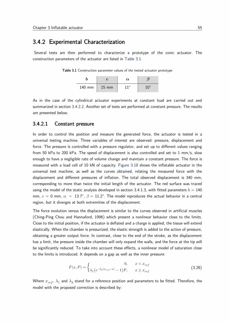
Chapter 3 Inflatable actuator 55

3.4.2 Experimental Characterization

Several tests are then performed to characterize a prototype of the conic actuator. The

construction parameters of the actuator are listed in Table 3.1.

Table 3.1 Construction parameter values of the tested actuator prototype

𝒃 𝒄 𝜶 𝜷

140 mm 15 mm 11° 10°

As in the case of the cylindrical actuator experiments at constant load are carried out and

summarized in section 3.4.2.2. Another set of tests are performed at constant pressure. The results

are presented below.

3.4.2.1 Constant pressure

In order to control the position and measure the generated force, the actuator is tested in a

universal testing machine. Three variables of interest are observed: pressure, displacement and

force. The pressure is controlled with a pressure regulator, and set up to different values ranging

from 50 kPa to 200 kPa. The speed of displacement is also controlled and set to 1 mm/s, slow

enough to have a negligible rate of volume change and maintain a constant pressure. The force is

measured with a load cell of 10 kN of capacity. Figure 3.18 shows the inflatable actuator in the

universal test machine, as well as the curves obtained, relating the measured force with the

displacement and different pressures of inflation. The total observed displacement is 340 mm,

corresponding to more than twice the initial length of the actuator. The red surface was traced

using the model of the static analysis developed in section 3.4.1.3, with fitted parameters 𝑏 = 140

mm, 𝑐 = 0 mm, 𝛼 = 13.7°, 𝛽 = 11.2°. The model reproduces the actual behavior in a central

region, but it diverges at both extremities of the displacement.

The force evolution versus the displacement is similar to the curves observed in artificial muscles

(Ching-Ping Chou and Hannaford, 1996) which present a nonlinear behavior close to the limits.

Close to the initial position, if the actuator is deflated and a charge is applied, the tissue will extend

elastically. When the chamber is pressurized, the elastic strength is added to the action of pressure,

obtaining a greater output force. In contrast, close to the end of the stroke, as the displacement

has a limit, the pressure inside the chamber will only expand the walls, and the force at the tip will

be significantly reduced. To take into account these effects, a nonlinear model of saturation close

to the limits is introduced. It depends on a gap as well as the inner pressure:

𝐹(𝑥, 𝑃 ) = {0, 𝑥 < 𝑥𝑟𝑒𝑓

𝜆1(𝑒−𝜆2(𝑥𝑟𝑒𝑓−𝑥) − 1)𝑃 , 𝑥 ≥ 𝑥𝑟𝑒𝑓

(3.28)

Where 𝑥𝑟𝑒𝑓 , 𝜆1 and 𝜆2 stand for a reference position and parameters to be fitted. Therefore, the

model with the proposed correction is described by:

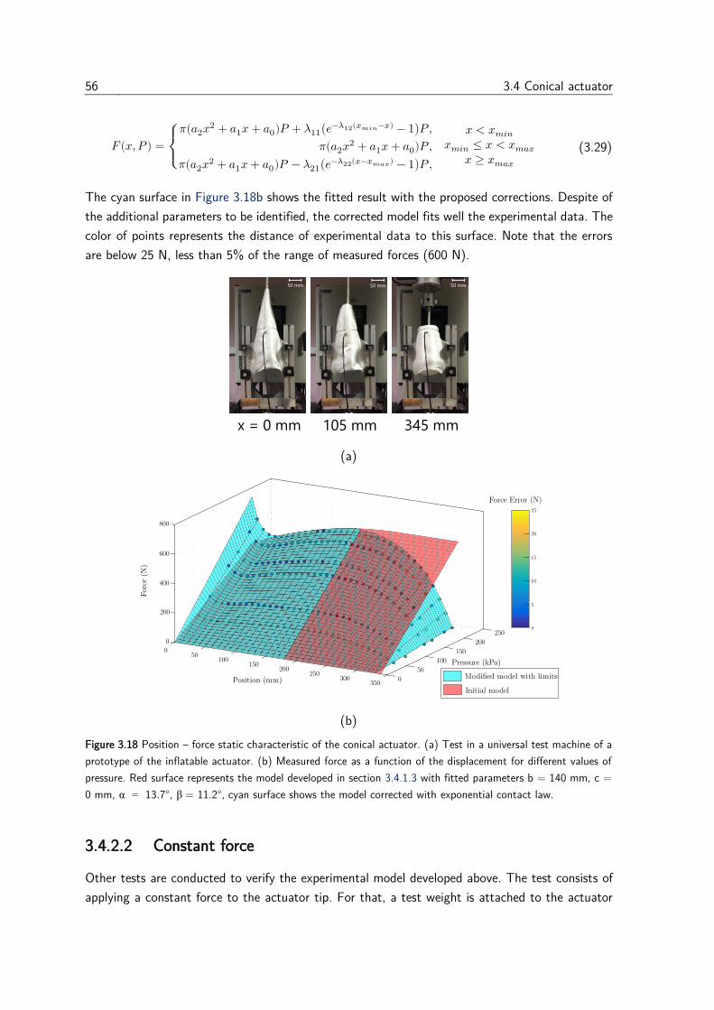
56 3.4 Conical actuator

𝐹(𝑥, 𝑃 ) =

{

𝜋(𝑎2𝑥

2 + 𝑎1𝑥 + 𝑎0)𝑃 + 𝜆11(𝑒−𝜆12(𝑥𝑚𝑖𝑛−𝑥) − 1)𝑃 ,

𝜋(𝑎2𝑥2 + 𝑎1𝑥 + 𝑎0)𝑃 ,

𝜋(𝑎2𝑥2 + 𝑎1𝑥 + 𝑎0)𝑃 − 𝜆21(𝑒

−𝜆22(𝑥−𝑥𝑚𝑎𝑥) − 1)𝑃 ,

𝑥 < 𝑥𝑚𝑖𝑛𝑥𝑚𝑖𝑛 ≤ 𝑥 < 𝑥𝑚𝑎𝑥𝑥 ≥ 𝑥𝑚𝑎𝑥

(3.29)

The cyan surface in Figure 3.18b shows the fitted result with the proposed corrections. Despite of

the additional parameters to be identified, the corrected model fits well the experimental data. The

color of points represents the distance of experimental data to this surface. Note that the errors

are below 25 N, less than 5% of the range of measured forces (600 N).

(a)

(b)

Figure 3.18 Position – force static characteristic of the conical actuator. (a) Test in a universal test machine of a

prototype of the inflatable actuator. (b) Measured force as a function of the displacement for different values of

pressure. Red surface represents the model developed in section 3.4.1.3 with fitted parameters b = 140 mm, c =

0 mm, α = 13.7°, β = 11.2°, cyan surface shows the model corrected with exponential contact law.

3.4.2.2 Constant force

Other tests are conducted to verify the experimental model developed above. The test consists of

applying a constant force to the actuator tip. For that, a test weight is attached to the actuator

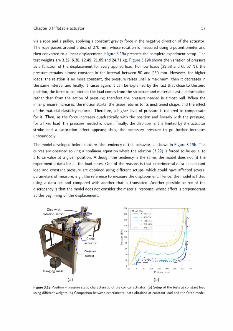
Chapter 3 Inflatable actuator 57

via a rope and a pulley, applying a constant gravity force in the negative direction of the actuator.

The rope passes around a disc of 270 mm, whose rotation is measured using a potentiometer and

then converted to a linear displacement. Figure 3.19a presents the complete experiment setup. The

test weights are 3.32, 6.38, 12.49, 21.65 and 24.71 kg. Figure 3.19b shows the variation of pressure

as a function of the displacement for every applied load. For low loads (32.58 and 65.57 N), the

pressure remains almost constant in the interval between 50 and 250 mm. However, for higher

loads, the relation is no more constant, the pressure raises until a maximum, then it decreases in

the same interval and finally, it raises again. It can be explained by the fact that close to the zero

position, the force to counteract the load comes from the structure and material elastic deformation

rather than from the action of pressure; therefore the pressure needed is almost null. When the

inner pressure increases, the motion starts, the tissue returns to its unstrained shape, and the effect

of the material elasticity reduces. Therefore, a higher level of pressure is required to compensate

for it. Then, as the force increases quadratically with the position and linearly with the pressure,

for a fixed load, the pressure needed is lower. Finally, the displacement is limited by the actuator

stroke and a saturation effect appears; thus, the necessary pressure to go further increases

unboundedly.

The model developed before captures the tendency of this behavior, as shown in Figure 3.19b. The

curves are obtained solving a nonlinear equation where the relation (3.29) is forced to be equal to

a force value at a given position. Although the tendency is the same, the model does not fit the

experimental data for all the load cases. One of the reasons is that experimental data at constant

load and constant pressure are obtained using different setups, which could have affected several

parameters of measure, e.g., the reference to measure the displacement. Hence, the model is fitted

using a data set and compared with another that is translated. Another possible source of the

discrepancy is that the model does not consider the material response, whose effect is preponderant

at the beginning of the displacement.

(a) (b)

Figure 3.19 Position – pressure static characteristic of the conical actuator. (a) Setup of the tests at constant load

using different weights (b) Comparison between experimental data obtained at constant load and the fitted model.

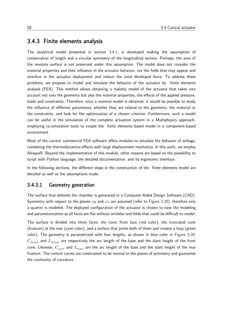
58 3.4 Conical actuator

3.4.3 Finite elements analysis

The analytical model presented in section 3.4.1, is developed making the assumption of

conservation of length and a circular symmetry of the longitudinal section. Perhaps, the area of

the revolute surface is not preserved under this assumption. The model does not consider the

material properties and their influence in the actuator behavior, nor the folds that may appear and

interfere in the actuator deployment and reduce the total developed force. To address these

problems, we propose to model and simulate the behavior of the actuator by finite elements

analysis (FEA). This method allows obtaining a realistic model of the actuator that takes into

account not only the geometry but also the material properties, the effects of the applied pressure,

loads and constraints. Therefore, once a nominal model is obtained, it would be possible to study

the influence of different parameters, whether they are related to the geometry, the material or

the constraints, and look for the optimization of a chosen criterion. Furthermore, such a model

can be useful in the simulation of the complete actuation system in a Multiphysics approach,

employing co-simulation tools to couple the finite elements based model in a component-based

environment.

Most of the current commercial FEA software offers modules to simulate the behavior of airbags,

combining the thermodynamics effects with large displacement mechanics. In this work, we employ

Abaqus®. Beyond the implementation of this module, other reasons are based on the possibility to

script with Python language, the detailed documentation, and its ergonomic interface.

In the following sections, the different steps in the construction of the finite elements model are

detailed as well as the assumptions made.

3.4.3.1 Geometry generation

The surface that delimits the chamber is generated in a Computer-Aided Design Software (CAD).

Symmetry with respect to the planes 𝑥𝑦 and 𝑥𝑧 are assumed (refer to Figure 3.20), therefore only

a quarter is modeled. The deployed configuration of the actuator is chosen to ease the modeling

and parameterization as all faces are flat without wrinkles and folds that could be difficult to model.

The surface is divided into three faces: the conic front face (red color), the truncated cone

(frustum) at the rear (cyan color), and a surface that joints both of them and creates a loop (green

color). The geometry is parametrized with four lengths, as shown in blue color in Figure 3.20:

𝐶𝑓𝑟𝑜𝑛𝑡 and 𝐿𝑓𝑟𝑜𝑛𝑡 are respectively the arc length of the base and the slant height of the front

cone. Likewise, 𝐶𝑟𝑒𝑎𝑟 and 𝐿𝑟𝑒𝑎𝑟 are the arc length of the base and the slant height of the rear

frustum. The control curves are constrained to be normal to the planes of symmetry and guarantee

the continuity of curvature.

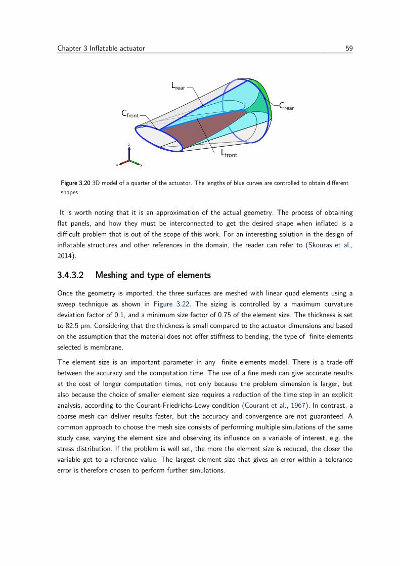
Chapter 3 Inflatable actuator 59

Figure 3.20 3D model of a quarter of the actuator. The lengths of blue curves are controlled to obtain different

shapes

It is worth noting that it is an approximation of the actual geometry. The process of obtaining

flat panels, and how they must be interconnected to get the desired shape when inflated is a

difficult problem that is out of the scope of this work. For an interesting solution in the design of

inflatable structures and other references in the domain, the reader can refer to (Skouras et al.,

2014).

3.4.3.2 Meshing and type of elements

Once the geometry is imported, the three surfaces are meshed with linear quad elements using a

sweep technique as shown in Figure 3.22. The sizing is controlled by a maximum curvature

deviation factor of 0.1, and a minimum size factor of 0.75 of the element size. The thickness is set

to 82.5 µm. Considering that the thickness is small compared to the actuator dimensions and based

on the assumption that the material does not offer stiffness to bending, the type of finite elements

selected is membrane.

The element size is an important parameter in any finite elements model. There is a trade-off

between the accuracy and the computation time. The use of a fine mesh can give accurate results

at the cost of longer computation times, not only because the problem dimension is larger, but

also because the choice of smaller element size requires a reduction of the time step in an explicit

analysis, according to the Courant-Friedrichs-Lewy condition (Courant et al., 1967). In contrast, a

coarse mesh can deliver results faster, but the accuracy and convergence are not guaranteed. A

common approach to choose the mesh size consists of performing multiple simulations of the same

study case, varying the element size and observing its influence on a variable of interest, e.g. the

stress distribution. If the problem is well set, the more the element size is reduced, the closer the

variable get to a reference value. The largest element size that gives an error within a tolerance

error is therefore chosen to perform further simulations.

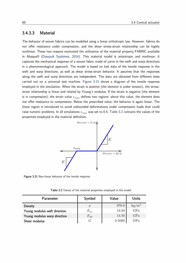
60 3.4 Conical actuator

3.4.3.3 Material

The behavior of woven fabrics can be modelled using a linear orthotropic law. However, fabrics do

not offer resistance under compression, and the shear stress-strain relationship can be highly

nonlinear. These two reasons motivated the utilization of the material property FABRIC available

in Abaqus® (Dassault Systèmes, 2014). This material model is anisotropic and nonlinear; it

captures the mechanical response of a woven fabric made of yarns in the weft and warp directions

in a phenomenological approach. The model is based on test data of the tensile response in the

weft and warp directions, as well as shear stress-strain behavior. It assumes that the responses

along the weft and warp directions are independent. The data are obtained from different tests

carried out on a universal test machine. Figure 3.21 shows a diagram of the tensile response

employed in the simulation. When the strain is positive (the element is under tension), the stress-

strain relationship is linear and related by Young’s modulus. If the strain is negative (the element

is in compression), the strain value 𝜖𝑚𝑖𝑛 defines two regions: above this value, the element does

not offer resistance to compression. Below the prescribed value, the behavior is again linear. The

linear region is introduced to avoid unbounded deformations under compression loads that could

raise numeric problems. In all simulations 𝜖𝑚𝑖𝑛 was set to 0.5. Table 3.2 contains the values of the

properties employed in the material definition.

Figure 3.21 Non-linear behavior of the tensile response

Table 3.2 Values of the material properties employed in the model

Parameter Symbol Value Units

Density 𝜌 970.0 kg/m3

Young modulus weft direction 𝐸11 13.50 GPa

Young modulus warp direction 𝐸22 14.50 GPa

Shear modulus 𝐺 0.5000 GPa

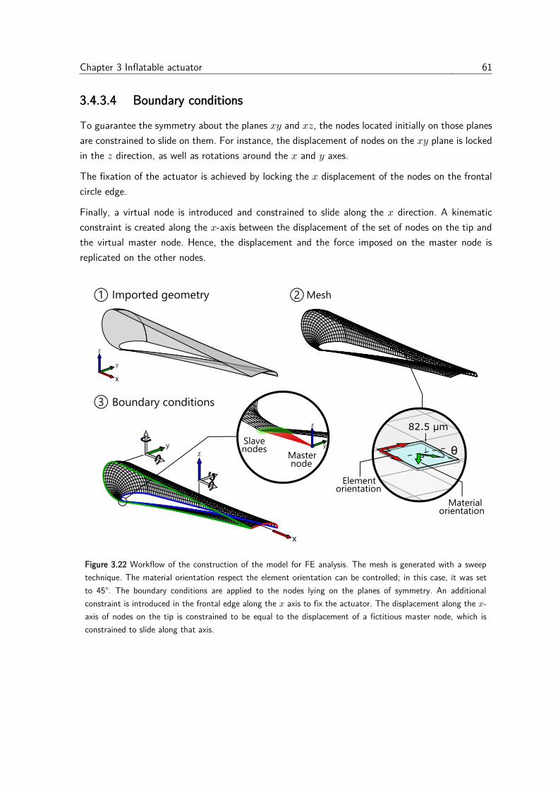
Chapter 3 Inflatable actuator 61

3.4.3.4 Boundary conditions

To guarantee the symmetry about the planes 𝑥𝑦 and 𝑥𝑧, the nodes located initially on those planes

are constrained to slide on them. For instance, the displacement of nodes on the 𝑥𝑦 plane is locked

in the 𝑧 direction, as well as rotations around the 𝑥 and 𝑦 axes.

The fixation of the actuator is achieved by locking the 𝑥 displacement of the nodes on the frontal

circle edge.

Finally, a virtual node is introduced and constrained to slide along the 𝑥 direction. A kinematic

constraint is created along the 𝑥-axis between the displacement of the set of nodes on the tip and

the virtual master node. Hence, the displacement and the force imposed on the master node is

replicated on the other nodes.

Figure 3.22 Workflow of the construction of the model for FE analysis. The mesh is generated with a sweep

technique. The material orientation respect the element orientation can be controlled; in this case, it was set

to 45°. The boundary conditions are applied to the nodes lying on the planes of symmetry. An additional

constraint is introduced in the frontal edge along the 𝑥 axis to fix the actuator. The displacement along the 𝑥-

axis of nodes on the tip is constrained to be equal to the displacement of a fictitious master node, which is

constrained to slide along that axis.

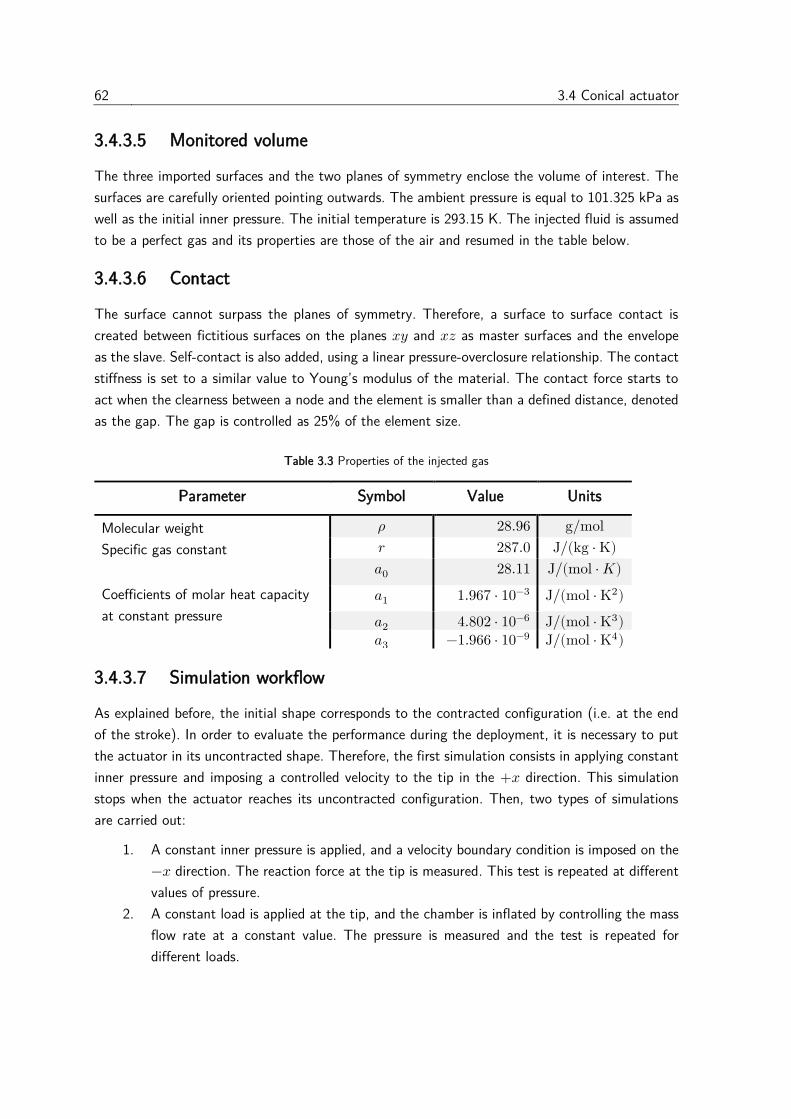
62 3.4 Conical actuator

3.4.3.5 Monitored volume

The three imported surfaces and the two planes of symmetry enclose the volume of interest. The

surfaces are carefully oriented pointing outwards. The ambient pressure is equal to 101.325 kPa as

well as the initial inner pressure. The initial temperature is 293.15 K. The injected fluid is assumed

to be a perfect gas and its properties are those of the air and resumed in the table below.

3.4.3.6 Contact

The surface cannot surpass the planes of symmetry. Therefore, a surface to surface contact is

created between fictitious surfaces on the planes 𝑥𝑦 and 𝑥𝑧 as master surfaces and the envelope

as the slave. Self-contact is also added, using a linear pressure-overclosure relationship. The contact

stiffness is set to a similar value to Young’s modulus of the material. The contact force starts to

act when the clearness between a node and the element is smaller than a defined distance, denoted

as the gap. The gap is controlled as 25% of the element size.

Table 3.3 Properties of the injected gas

Parameter Symbol Value Units

Molecular weight 𝜌 28.96 g/mol

Specific gas constant 𝑟 287.0 J/(kg ⋅ K)

Coefficients of molar heat capacity

at constant pressure

𝑎0 28.11 J/(mol ⋅ 𝐾)

𝑎1 1.967 ⋅ 10−3 J/(mol ⋅ K2)

𝑎2 4.802 ⋅ 10−6 J/(mol ⋅ K3) 𝑎3 −1.966 ⋅ 10−9 J/(mol ⋅ K4)

3.4.3.7 Simulation workflow

As explained before, the initial shape corresponds to the contracted configuration (i.e. at the end

of the stroke). In order to evaluate the performance during the deployment, it is necessary to put

the actuator in its uncontracted shape. Therefore, the first simulation consists in applying constant

inner pressure and imposing a controlled velocity to the tip in the +𝑥 direction. This simulation

stops when the actuator reaches its uncontracted configuration. Then, two types of simulations

are carried out:

1. A constant inner pressure is applied, and a velocity boundary condition is imposed on the

−𝑥 direction. The reaction force at the tip is measured. This test is repeated at different

values of pressure.

2. A constant load is applied at the tip, and the chamber is inflated by controlling the mass

flow rate at a constant value. The pressure is measured and the test is repeated for

different loads.

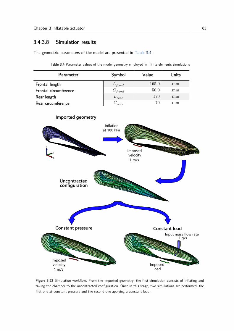
Chapter 3 Inflatable actuator 63

3.4.3.8 Simulation results

The geometric parameters of the model are presented in Table 3.4.

Table 3.4 Parameter values of the model geometry employed in finite elements simulations

Parameter Symbol Value Units

Frontal length 𝐿𝑓𝑟𝑜𝑛𝑡 165.0 mm

Frontal circumference 𝐶𝑓𝑟𝑜𝑛𝑡 50.0 mm

Rear length 𝐿𝑟𝑒𝑎𝑟 170 mm

Rear circumference 𝐶𝑟𝑒𝑎𝑟 70 mm

Figure 3.23 Simulation workflow. From the imported geometry, the first simulation consists of inflating and

taking the chamber to the uncontracted configuration. Once in this stage, two simulations are performed, the

first one at constant pressure and the second one applying a constant load.

64 3.4 Conical actuator

The mesh size was set to 3 mm, giving a total of 2014 nodes and 1876 membrane elements,

representing a total of 6097 degrees of freedom, including Lagrange multipliers for contact. The

first simulation of inflation at 180 kPa followed by a controlled motion at a constant velocity of 1

m/s allows obtaining the geometry with the front face deployed and the rear surface everted. From

this configuration, the first set of tests consists in raising the pressure from the atmospheric pressure

to a constant value. This transition is performed rapidly (in 0.01 s, see Figure 3.24) because the

transient response is not of interest in this analysis. Then, the tip starts to move with a velocity of

1 m/s, and the reaction force is measured at the same point. The motion is maintained during

0.415 s, completing a total displacement of 300 mm. Once stopped, the inner pressure regains the

atmospheric value. This protocol is repeated for the following values of source pressures: 50, 80

and 130 kPa.

Figure 3.24 Velocity and pressure profiles in FE simulations.

Figure 3.25 shows the results relating the measured force to the displacement. As only a quarter

of the surface is considered, and making the assumption that the behaviour is equal in the other

quarters, the force obtained is four times higher. Therefore, the results of the force are multiplied

by 4. Note that the curves do not start at 0 mm but at 22.5 mm. The reason is that in the first

step, when the actuator is put in the initial configuration, forcing a displacement until 0 mm caused

high strains and stresses in elements close to the tip. Therefore, the total displacement has to be

reduced to get a stable geometry for the following step.

=P

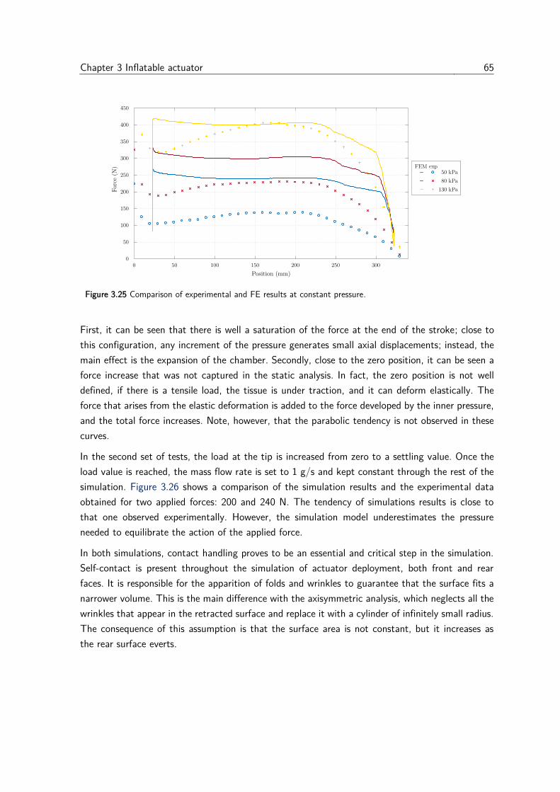
Chapter 3 Inflatable actuator 65

Figure 3.25 Comparison of experimental and FE results at constant pressure.

First, it can be seen that there is well a saturation of the force at the end of the stroke; close to

this configuration, any increment of the pressure generates small axial displacements; instead, the

main effect is the expansion of the chamber. Secondly, close to the zero position, it can be seen a

force increase that was not captured in the static analysis. In fact, the zero position is not well

defined, if there is a tensile load, the tissue is under traction, and it can deform elastically. The

force that arises from the elastic deformation is added to the force developed by the inner pressure,

and the total force increases. Note, however, that the parabolic tendency is not observed in these

curves.

In the second set of tests, the load at the tip is increased from zero to a settling value. Once the

load value is reached, the mass flow rate is set to 1 g/s and kept constant through the rest of the

simulation. Figure 3.26 shows a comparison of the simulation results and the experimental data

obtained for two applied forces: 200 and 240 N. The tendency of simulations results is close to

that one observed experimentally. However, the simulation model underestimates the pressure

needed to equilibrate the action of the applied force.

In both simulations, contact handling proves to be an essential and critical step in the simulation.

Self-contact is present throughout the simulation of actuator deployment, both front and rear

faces. It is responsible for the apparition of folds and wrinkles to guarantee that the surface fits a

narrower volume. This is the main difference with the axisymmetric analysis, which neglects all the

wrinkles that appear in the retracted surface and replace it with a cylinder of infinitely small radius.

The consequence of this assumption is that the surface area is not constant, but it increases as

the rear surface everts.

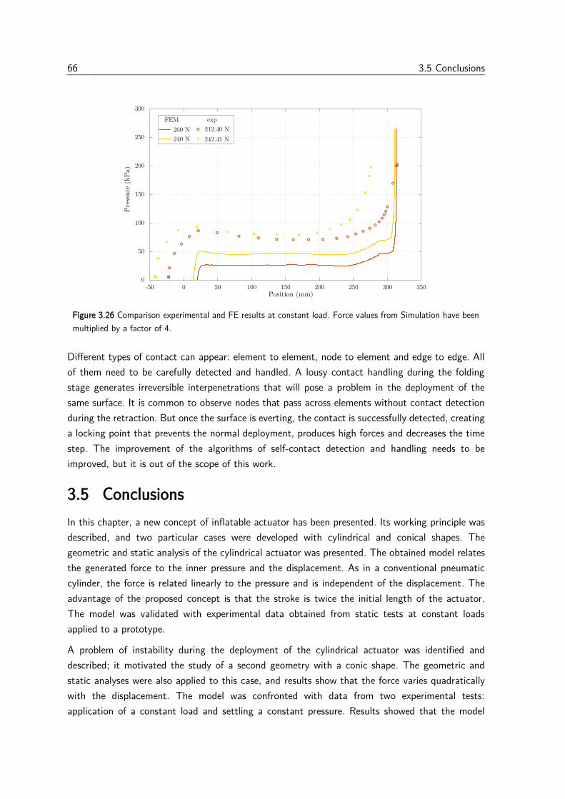
66 3.5 Conclusions

Figure 3.26 Comparison experimental and FE results at constant load. Force values from Simulation have been

multiplied by a factor of 4.

Different types of contact can appear: element to element, node to element and edge to edge. All

of them need to be carefully detected and handled. A lousy contact handling during the folding

stage generates irreversible interpenetrations that will pose a problem in the deployment of the

same surface. It is common to observe nodes that pass across elements without contact detection

during the retraction. But once the surface is everting, the contact is successfully detected, creating

a locking point that prevents the normal deployment, produces high forces and decreases the time

step. The improvement of the algorithms of self-contact detection and handling needs to be

improved, but it is out of the scope of this work.

3.5 Conclusions

In this chapter, a new concept of inflatable actuator has been presented. Its working principle was

described, and two particular cases were developed with cylindrical and conical shapes. The

geometric and static analysis of the cylindrical actuator was presented. The obtained model relates

the generated force to the inner pressure and the displacement. As in a conventional pneumatic

cylinder, the force is related linearly to the pressure and is independent of the displacement. The

advantage of the proposed concept is that the stroke is twice the initial length of the actuator.

The model was validated with experimental data obtained from static tests at constant loads

applied to a prototype.

A problem of instability during the deployment of the cylindrical actuator was identified and

described; it motivated the study of a second geometry with a conic shape. The geometric and

static analyses were also applied to this case, and results show that the force varies quadratically

with the displacement. The model was confronted with data from two experimental tests:

application of a constant load and settling a constant pressure. Results showed that the model

Chapter 3 Inflatable actuator 67

captures the behavior in a range of the total stroke, but diverges close to the limits where the

saturation effects are predominant but were not taken into account. The model was modified by

introducing contact-like exponential laws that fitted better experimental data.

In order to take into account the effects of fixation points, material properties and possible folds

that can appear during the actuator deployment, an approach based on finite elements simulation

was proposed. The method covered the geometry generation, the finite elements model preparation

and the execution. Like in the experimental tests, two types of simulations were carried out: the

first one considered a constant pressure while the other one assumed the application of a constant

force. Results showed that the tendencies of the curves obtained by simulation follow the same

behavior observed in experimental tests. However, further work needs to focus on the parameter

tuning of finite elements simulations to obtain a response closer to that one observed in

experiments. Some of the parameters whose influence needs to be explored in more detail are the

tensile and shear modulus. As proposed in section 3.4.3.3, the material responses (tensile and

shear) can be defined by non-linear stress-strain relationships. Furthermore, it is possible to define

different loading and unloading curves to include hysteresis effects. The modification of these curves

can have a significant impact and improve the results obtained. Further experimental campaigns

in the characterization of the material could be carried out to have a better estimation of these

properties. It would be suitable to use specialized equipment for tissue characterization, such as a

biaxial testing machine.

The refinement of the finite elements model will be a key step to continue multiple developments:

by modifying the properties of the elements on the edges, the behavior of the sewings could be

taken into account and analyze their effect in the stress concentration. Another axis of development

is the optimization of the shape: as it was introduced in the actuator description, the curve that

generates the volume is required to be monotonically increasing. We have explored constant and

linear curves, but other shapes could be explored to improve the force-displacement characteristic.

The study of the geometry of the rear surface, joining the actuator tip to the major surface, has

been skipped in this work, but it plays a critical role, for instance, in the shape determination of

the rear cross-section when the actuator is inflated completely.

Evidence shows that the majority of leakages and failures are located close to the sewings. One of

the reasons is that the woven polyethylene fibers are very smooth and can slide easily one over the

others, especially those close to the sewings where the stress concentration is higher. When two

parallel fibers slide, they leave a series of hollows (such as in a strainer) where the airtight inner

layer will accommodate by the effect of the pressure. The holes do not disappear after venting,

and they become stress raisers for the inner layer.

The work presented in this chapter goes beyond the analysis and study of the performance of this

original actuator. It is also intended to provide a tool for feedback on the design of the actuator in

order to improve its capabilities and adapt it to other applications.

Chapter 4

Sensors for inflatable robots

All our knowledge begins with the senses, proceeds

then to the understanding, and ends with reason.

There is nothing higher than reason

― Immanuel Kant, Critique of Pure Reason

Contents

4.1 Introduction ..................................................................................................... 70

4.2 State of the art ................................................................................................ 71

4.2.1 Resistive sensors ......................................................................................... 71

4.2.2 Capacitive stretch sensors ........................................................................... 74

4.2.3 Fiber optic sensors ...................................................................................... 75

4.2.4 MEMS inertial sensors ................................................................................ 76

4.2.5 External sensors .......................................................................................... 77

4.3 Sensor choice ................................................................................................... 78

4.4 Background notions: Rigid body rotation ............................................................ 79

4.4.1 Quaternion definition .................................................................................. 79

4.4.2 Unit quaternions as rotation operators ......................................................... 80

4.5 Proposed approaches......................................................................................... 82

4.5.1 Perturbed magnetic sensors ......................................................................... 82

4.5.2 Relative orientation data fusion ................................................................... 89

4.6 Relative orientation between rigid bodies ............................................................ 99

4.7 Conclusions ..................................................................................................... 100

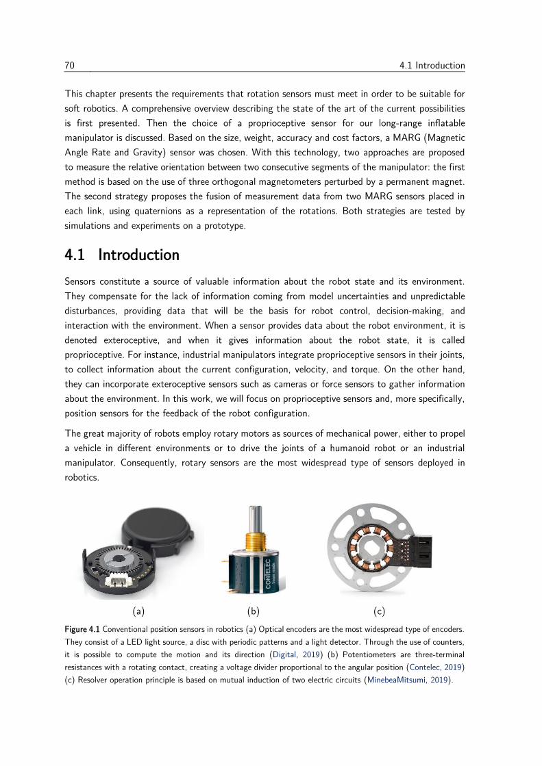
70 4.1 Introduction

This chapter presents the requirements that rotation sensors must meet in order to be suitable for

soft robotics. A comprehensive overview describing the state of the art of the current possibilities

is first presented. Then the choice of a proprioceptive sensor for our long-range inflatable

manipulator is discussed. Based on the size, weight, accuracy and cost factors, a MARG (Magnetic

Angle Rate and Gravity) sensor was chosen. With this technology, two approaches are proposed

to measure the relative orientation between two consecutive segments of the manipulator: the first

method is based on the use of three orthogonal magnetometers perturbed by a permanent magnet.

The second strategy proposes the fusion of measurement data from two MARG sensors placed in

each link, using quaternions as a representation of the rotations. Both strategies are tested by

simulations and experiments on a prototype.

4.1 Introduction

Sensors constitute a source of valuable information about the robot state and its environment.

They compensate for the lack of information coming from model uncertainties and unpredictable

disturbances, providing data that will be the basis for robot control, decision-making, and

interaction with the environment. When a sensor provides data about the robot environment, it is

denoted exteroceptive, and when it gives information about the robot state, it is called

proprioceptive. For instance, industrial manipulators integrate proprioceptive sensors in their joints,

to collect information about the current configuration, velocity, and torque. On the other hand,

they can incorporate exteroceptive sensors such as cameras or force sensors to gather information

about the environment. In this work, we will focus on proprioceptive sensors and, more specifically,

position sensors for the feedback of the robot configuration.

The great majority of robots employ rotary motors as sources of mechanical power, either to propel

a vehicle in different environments or to drive the joints of a humanoid robot or an industrial

manipulator. Consequently, rotary sensors are the most widespread type of sensors deployed in

robotics.

(a) (b) (c)

Figure 4.1 Conventional position sensors in robotics (a) Optical encoders are the most widespread type of encoders.

They consist of a LED light source, a disc with periodic patterns and a light detector. Through the use of counters,

it is possible to compute the motion and its direction (Digital, 2019) (b) Potentiometers are three-terminal

resistances with a rotating contact, creating a voltage divider proportional to the angular position (Contelec, 2019)

(c) Resolver operation principle is based on mutual induction of two electric circuits (MinebeaMitsumi, 2019).

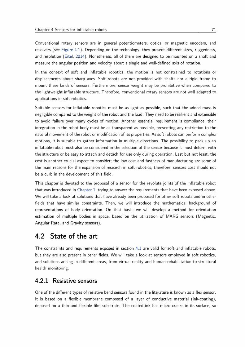
Chapter 4 Sensors for inflatable robots 71

Conventional rotary sensors are in general potentiometers, optical or magnetic encoders, and

resolvers (see Figure 4.1). Depending on the technology, they present different sizes, ruggedness,

and resolution (Eitel, 2014). Nonetheless, all of them are designed to be mounted on a shaft and

measure the angular position and velocity about a single and well-defined axis of rotation.

In the context of soft and inflatable robotics, the motion is not constrained to rotations or

displacements about sharp axes. Soft robots are not provided with shafts nor a rigid frame to

mount these kinds of sensors. Furthermore, sensor weight may be prohibitive when compared to

the lightweight inflatable structure. Therefore, conventional rotary sensors are not well adapted to

applications in soft robotics.

Suitable sensors for inflatable robotics must be as light as possible, such that the added mass is

negligible compared to the weight of the robot and the load. They need to be resilient and extensible

to avoid failure over many cycles of motion. Another essential requirement is compliance: their

integration in the robot body must be as transparent as possible, preventing any restriction to the

natural movement of the robot or modification of its properties. As soft robots can perform complex

motions, it is suitable to gather information in multiple directions. The possibility to pack up an

inflatable robot must also be considered in the selection of the sensor because it must deform with

the structure or be easy to attach and detach for use only during operation. Last but not least, the

cost is another crucial aspect to consider; the low cost and fastness of manufacturing are some of

the main reasons for the expansion of research in soft robotics; therefore, sensors cost should not

be a curb in the development of this field.

This chapter is devoted to the proposal of a sensor for the revolute joints of the inflatable robot

that was introduced in Chapter 1, trying to answer the requirements that have been exposed above.

We will take a look at solutions that have already been proposed for other soft robots and in other

fields that have similar constraints. Then, we will introduce the mathematical background of

representations of body orientation. On that basis, we will develop a method for orientation

estimation of multiple bodies in space, based on the utilization of MARG sensors (Magnetic,

Angular Rate, and Gravity sensors).

4.2 State of the art

The constraints and requirements exposed in section 4.1 are valid for soft and inflatable robots,

but they are also present in other fields. We will take a look at sensors employed in soft robotics,

and solutions arising in different areas, from virtual reality and human rehabilitation to structural

health monitoring.

4.2.1 Resistive sensors

One of the different types of resistive bend sensors found in the literature is known as a flex sensor.

It is based on a flexible membrane composed of a layer of conductive material (ink-coating),

deposed on a thin and flexible film substrate. The coated-ink has micro-cracks in its surface, so

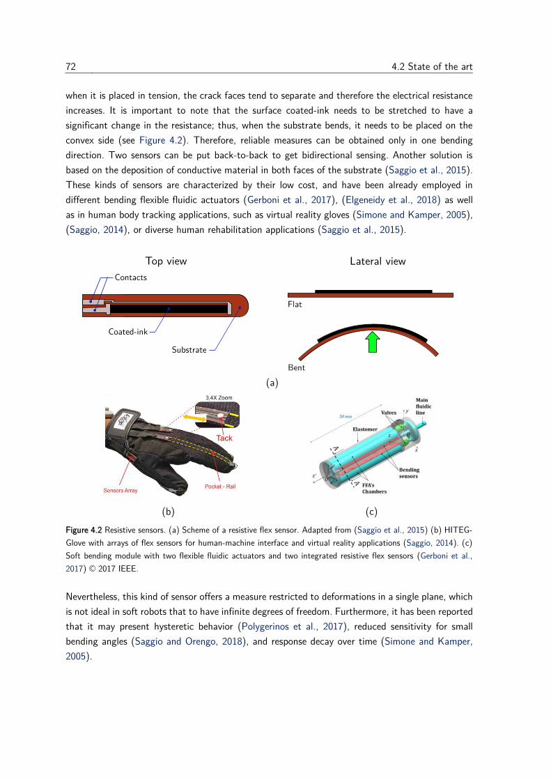
72 4.2 State of the art

when it is placed in tension, the crack faces tend to separate and therefore the electrical resistance

increases. It is important to note that the surface coated-ink needs to be stretched to have a

significant change in the resistance; thus, when the substrate bends, it needs to be placed on the

convex side (see Figure 4.2). Therefore, reliable measures can be obtained only in one bending

direction. Two sensors can be put back-to-back to get bidirectional sensing. Another solution is

based on the deposition of conductive material in both faces of the substrate (Saggio et al., 2015).

These kinds of sensors are characterized by their low cost, and have been already employed in

different bending flexible fluidic actuators (Gerboni et al., 2017), (Elgeneidy et al., 2018) as well

as in human body tracking applications, such as virtual reality gloves (Simone and Kamper, 2005),

(Saggio, 2014), or diverse human rehabilitation applications (Saggio et al., 2015).

(a)

(b) (c)

Figure 4.2 Resistive sensors. (a) Scheme of a resistive flex sensor. Adapted from (Saggio et al., 2015) (b) HITEG-

Glove with arrays of flex sensors for human-machine interface and virtual reality applications (Saggio, 2014). (c)

Soft bending module with two flexible fluidic actuators and two integrated resistive flex sensors (Gerboni et al.,

2017) © 2017 IEEE.

Nevertheless, this kind of sensor offers a measure restricted to deformations in a single plane, which

is not ideal in soft robots that to have infinite degrees of freedom. Furthermore, it has been reported

that it may present hysteretic behavior (Polygerinos et al., 2017), reduced sensitivity for small

bending angles (Saggio and Orengo, 2018), and response decay over time (Simone and Kamper,

2005).

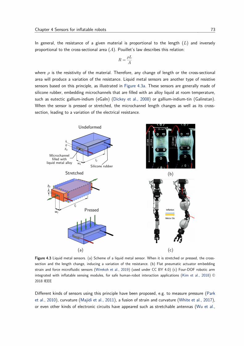
Chapter 4 Sensors for inflatable robots 73

In general, the resistance of a given material is proportional to the length (𝐿) and inversely

proportional to the cross-sectional area (𝐴). Pouillet’s law describes this relation:

𝑅 =𝜌𝐿

𝐴

where 𝜌 is the resistivity of the material. Therefore, any change of length or the cross-sectional

area will produce a variation of the resistance. Liquid metal sensors are another type of resistive

sensors based on this principle, as illustrated in Figure 4.3a. These sensors are generally made of

silicone rubber, embedding microchannels that are filled with an alloy liquid at room temperature,

such as eutectic gallium-indium (eGaIn) (Dickey et al., 2008) or gallium-indium-tin (Galinstan).

When the sensor is pressed or stretched, the microchannel length changes as well as its cross-

section, leading to a variation of the electrical resistance.

(b)

(a) (c)

Figure 4.3 Liquid metal sensors. (a) Scheme of a liquid metal sensor. When it is stretched or pressed, the cross-

section and the length change, inducing a variation of the resistance. (b) Flat pneumatic actuator embedding

strain and force microfluidic sensors (Wirekoh et al., 2019) (used under CC BY 4.0) (c) Four-DOF robotic arm

integrated with inflatable sensing modules, for safe human-robot interaction applications (Kim et al., 2018) ©

2018 IEEE

Different kinds of sensors using this principle have been proposed, e.g. to measure pressure (Park

et al., 2010), curvature (Majidi et al., 2011), a fusion of strain and curvature (White et al., 2017),

or even other kinds of electronic circuits have appeared such as stretchable antennas (Wu et al.,

74 4.2 State of the art

2015). One of the advantages of this sensor is the direct integration in soft actuators as a strain

or pressure sensor (Wirekoh et al., 2019), or in the robot structure, to gather information of the

environment through touch (Yin et al., 2017) or contact and impact detection (Kim et al., 2018).

However, there are still certain limitations on the applicability of liquid metal sensors to soft

robotics. Fabrication of microchannels is challenging, it relies on methods such as photolithography

or specialized printing hardware that can be costly and time-consuming. Although their relative

response in terms of resistance is reliable, the absolute variation between the unbent and the fully

bent configuration remains small, due to the high conductivity of eGaIn. Therefore, the sensor

sensitivity to noise is still high. On the other hand, most of these sensors are completely wired in

eGaIn; thus, any external stimulus applied out of the sensitive area will induce a change in the

geometry and could be interpreted as a strain. Finally, in applications such as minimally invasive

surgery, the use of eGaIn raises a problem of biocompatibility. Therefore, other conductive liquids

such as saline solutions have been explored(Russo et al., 2015).

4.2.2 Capacitive stretch sensors

Capacitance variations in a deformable structure is another way to measure strains. A capacitor is

composed of two conductive layers separated by an insulator material known as dielectric; when a

potential difference (voltage) is applied to both plates, a concentration of opposite electric charges

appears on every side. The capacitance is the ratio between the electrical charge in plates and the

applied tension. In a plate capacitor, the capacitance is related to the geometry and properties of

the electrodes by

𝐶 = 𝜖𝑟𝜖0𝐴

𝑑

where 𝐴 and 𝑑 are respectively the area of overlap and the separation between two electrodes, 𝜖𝑟

is the dielectric constant, and 𝜖0 is the electric constant (Hayt and Buck, 2001). Hence, any change

of the area or the separation between both electrodes will result in a variation of the capacitance.

An approach to create capacitive sensors is to use stretchable electrodes, separated by an elastomer

film as dielectric. When stretched, the electrodes and the dielectric deform, electrodes approach

one to the other, and the overlap area changes, modifying the capacitance as well. This approach,

known as dielectric elastomer sensors (DES) is not new, in 1880 Röntgen had already employed

natural rubber with sprayed-on electrostatic charges to study the effects of electric fields in

elastomer deformations (Röntgen, 1880), giving the basis of current dielectric elastomer actuators

(DEAs) (Pelrine et al., 2000). The dielectric is often made of silicone elastomer as well as the

electrodes, and the conductivity is assured embedding conductive carbon particles (carbon black

powder) (Rosset and Shea, 2013). The low elastic modulus of silicone (around 1 MPa) leads to

highly stretchable sensors that impart minimal change on the impedance of the structure where

deformation is measured. Moreover, dielectric elastomer sensors have shown better performances

than resistive sensors in terms of reliable signals over long periods and no hysteresis effects

(Litteken, 2017). Dielectric elastomer sensors are already produced and commercialized in

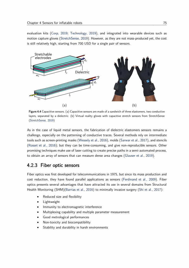
Chapter 4 Sensors for inflatable robots 75

evaluation kits (Corp, 2019; Technology, 2019), and integrated into wearable devices such as

motion capture gloves (StretchSense, 2019). However, as they are not mass-produced yet, the cost

is still relatively high, starting from 700 USD for a single pair of sensors.

(a) (b)

Figure 4.4 Capacitive sensors. (a) Capacitive sensors are made of a sandwich of three elastomers, two conductive

layers, separated by a dielectric. (b) Virtual reality gloves with capacitive stretch sensors from StretchSense

(StretchSense, 2019)

As in the case of liquid metal sensors, the fabrication of dielectric elastomers sensors remains a

challenge, especially on the patterning of conductive traces. Several methods rely on intermediate

tools such as screen-printing masks (Wessely et al., 2016), molds (Sarwar et al., 2017), and stencils

(Rosset et al., 2016); but they can be time-consuming, and give non-reproducible sensors. Other

promising techniques make use of laser cutting to create precise paths in a semi-automated process,

to obtain an array of sensors that can measure dense area changes (Glauser et al., 2019).

4.2.3 Fiber optic sensors

Fiber optics was first developed for telecommunications in 1975, but since its mass production and

cost reduction, they have found parallel applications as sensors (Ferdinand et al., 2009). Fiber

optics presents several advantages that have attracted its use in several domains from Structural

Health Monitoring (SHM)(Barrias et al., 2016) to minimally invasive surgery (Shi et al., 2017):

• Reduced size and flexibility

• Lightweight

• Immunity to electromagnetic interference

• Multiplexing capability and multiple parameter measurement

• Good metrological performances

• Non-toxicity and biocompatibility

• Stability and durability in harsh environments

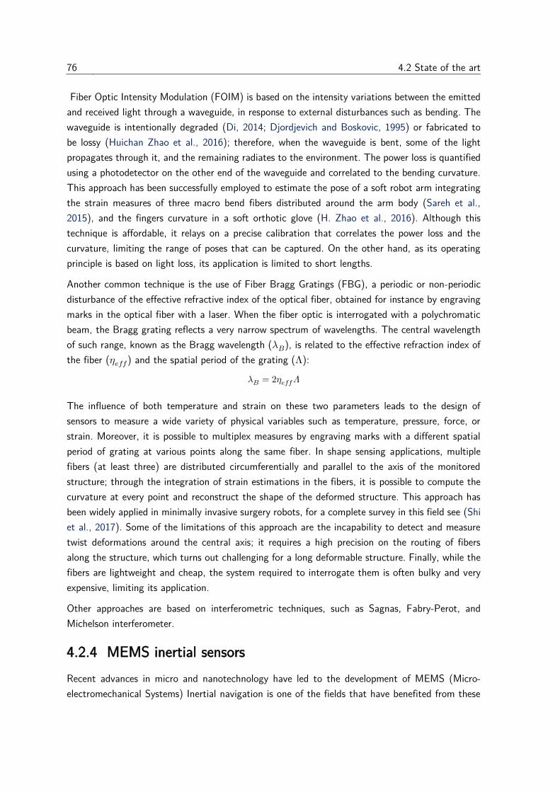
76 4.2 State of the art

Fiber Optic Intensity Modulation (FOIM) is based on the intensity variations between the emitted

and received light through a waveguide, in response to external disturbances such as bending. The

waveguide is intentionally degraded (Di, 2014; Djordjevich and Boskovic, 1995) or fabricated to

be lossy (Huichan Zhao et al., 2016); therefore, when the waveguide is bent, some of the light

propagates through it, and the remaining radiates to the environment. The power loss is quantified

using a photodetector on the other end of the waveguide and correlated to the bending curvature.

This approach has been successfully employed to estimate the pose of a soft robot arm integrating

the strain measures of three macro bend fibers distributed around the arm body (Sareh et al.,

2015), and the fingers curvature in a soft orthotic glove (H. Zhao et al., 2016). Although this

technique is affordable, it relays on a precise calibration that correlates the power loss and the

curvature, limiting the range of poses that can be captured. On the other hand, as its operating

principle is based on light loss, its application is limited to short lengths.

Another common technique is the use of Fiber Bragg Gratings (FBG), a periodic or non-periodic

disturbance of the effective refractive index of the optical fiber, obtained for instance by engraving

marks in the optical fiber with a laser. When the fiber optic is interrogated with a polychromatic

beam, the Bragg grating reflects a very narrow spectrum of wavelengths. The central wavelength

of such range, known as the Bragg wavelength (𝜆𝐵), is related to the effective refraction index of

the fiber (𝜂𝑒𝑓𝑓) and the spatial period of the grating (Λ):

𝜆𝐵 = 2𝜂𝑒𝑓𝑓𝛬

The influence of both temperature and strain on these two parameters leads to the design of

sensors to measure a wide variety of physical variables such as temperature, pressure, force, or

strain. Moreover, it is possible to multiplex measures by engraving marks with a different spatial

period of grating at various points along the same fiber. In shape sensing applications, multiple

fibers (at least three) are distributed circumferentially and parallel to the axis of the monitored

structure; through the integration of strain estimations in the fibers, it is possible to compute the

curvature at every point and reconstruct the shape of the deformed structure. This approach has

been widely applied in minimally invasive surgery robots, for a complete survey in this field see (Shi

et al., 2017). Some of the limitations of this approach are the incapability to detect and measure

twist deformations around the central axis; it requires a high precision on the routing of fibers

along the structure, which turns out challenging for a long deformable structure. Finally, while the

fibers are lightweight and cheap, the system required to interrogate them is often bulky and very

expensive, limiting its application.

Other approaches are based on interferometric techniques, such as Sagnas, Fabry-Perot, and

Michelson interferometer.

4.2.4 MEMS inertial sensors

Recent advances in micro and nanotechnology have led to the development of MEMS (Micro-

electromechanical Systems) Inertial navigation is one of the fields that have benefited from these

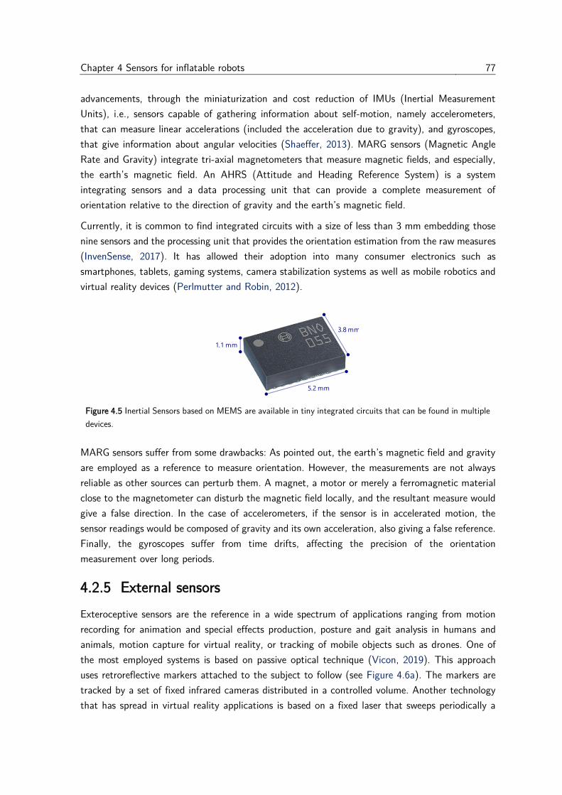
Chapter 4 Sensors for inflatable robots 77

advancements, through the miniaturization and cost reduction of IMUs (Inertial Measurement

Units), i.e., sensors capable of gathering information about self-motion, namely accelerometers,

that can measure linear accelerations (included the acceleration due to gravity), and gyroscopes,

that give information about angular velocities (Shaeffer, 2013). MARG sensors (Magnetic Angle

Rate and Gravity) integrate tri-axial magnetometers that measure magnetic fields, and especially,

the earth’s magnetic field. An AHRS (Attitude and Heading Reference System) is a system

integrating sensors and a data processing unit that can provide a complete measurement of

orientation relative to the direction of gravity and the earth’s magnetic field.

Currently, it is common to find integrated circuits with a size of less than 3 mm embedding those

nine sensors and the processing unit that provides the orientation estimation from the raw measures

(InvenSense, 2017). It has allowed their adoption into many consumer electronics such as

smartphones, tablets, gaming systems, camera stabilization systems as well as mobile robotics and

virtual reality devices (Perlmutter and Robin, 2012).

Figure 4.5 Inertial Sensors based on MEMS are available in tiny integrated circuits that can be found in multiple

devices.

MARG sensors suffer from some drawbacks: As pointed out, the earth’s magnetic field and gravity

are employed as a reference to measure orientation. However, the measurements are not always

reliable as other sources can perturb them. A magnet, a motor or merely a ferromagnetic material

close to the magnetometer can disturb the magnetic field locally, and the resultant measure would

give a false direction. In the case of accelerometers, if the sensor is in accelerated motion, the

sensor readings would be composed of gravity and its own acceleration, also giving a false reference.

Finally, the gyroscopes suffer from time drifts, affecting the precision of the orientation

measurement over long periods.

4.2.5 External sensors

Exteroceptive sensors are the reference in a wide spectrum of applications ranging from motion

recording for animation and special effects production, posture and gait analysis in humans and

animals, motion capture for virtual reality, or tracking of mobile objects such as drones. One of

the most employed systems is based on passive optical technique (Vicon, 2019). This approach

uses retroreflective markers attached to the subject to follow (see Figure 4.6a). The markers are

tracked by a set of fixed infrared cameras distributed in a controlled volume. Another technology

that has spread in virtual reality applications is based on a fixed laser that sweeps periodically a

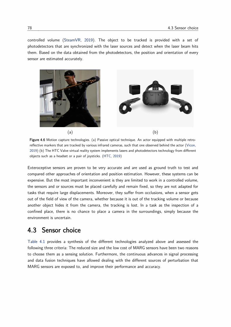
78 4.3 Sensor choice

controlled volume (SteamVR, 2019). The object to be tracked is provided with a set of

photodetectors that are synchronized with the laser sources and detect when the laser beam hits

them. Based on the data obtained from the photodetectors, the position and orientation of every

sensor are estimated accurately.

(a) (b)

Figure 4.6 Motion capture technologies. (a) Passive optical technique. An actor equipped with multiple retro-

reflective markers that are tracked by various infrared cameras, such that one observed behind the actor (Vicon,

2019) (b) The HTC Valve virtual reality system implements lasers and photodetectors technology from different

objects such as a headset or a pair of joysticks. (HTC, 2019)

Exteroceptive sensors are proven to be very accurate and are used as ground truth to test and

compared other approaches of orientation and position estimation. However, these systems can be

expensive. But the most important inconvenient is they are limited to work in a controlled volume,

the sensors and or sources must be placed carefully and remain fixed, so they are not adapted for

tasks that require large displacements. Moreover, they suffer from occlusions, when a sensor gets

out of the field of view of the camera, whether because it is out of the tracking volume or because

another object hides it from the camera, the tracking is lost. In a task as the inspection of a

confined place, there is no chance to place a camera in the surroundings, simply because the

environment is uncertain.

4.3 Sensor choice

Table 4.1 provides a synthesis of the different technologies analyzed above and assessed the

following three criteria: The reduced size and the low cost of MARG sensors have been two reasons

to choose them as a sensing solution. Furthermore, the continuous advances in signal processing

and data fusion techniques have allowed dealing with the different sources of perturbation that

MARG sensors are exposed to, and improve their performance and accuracy.

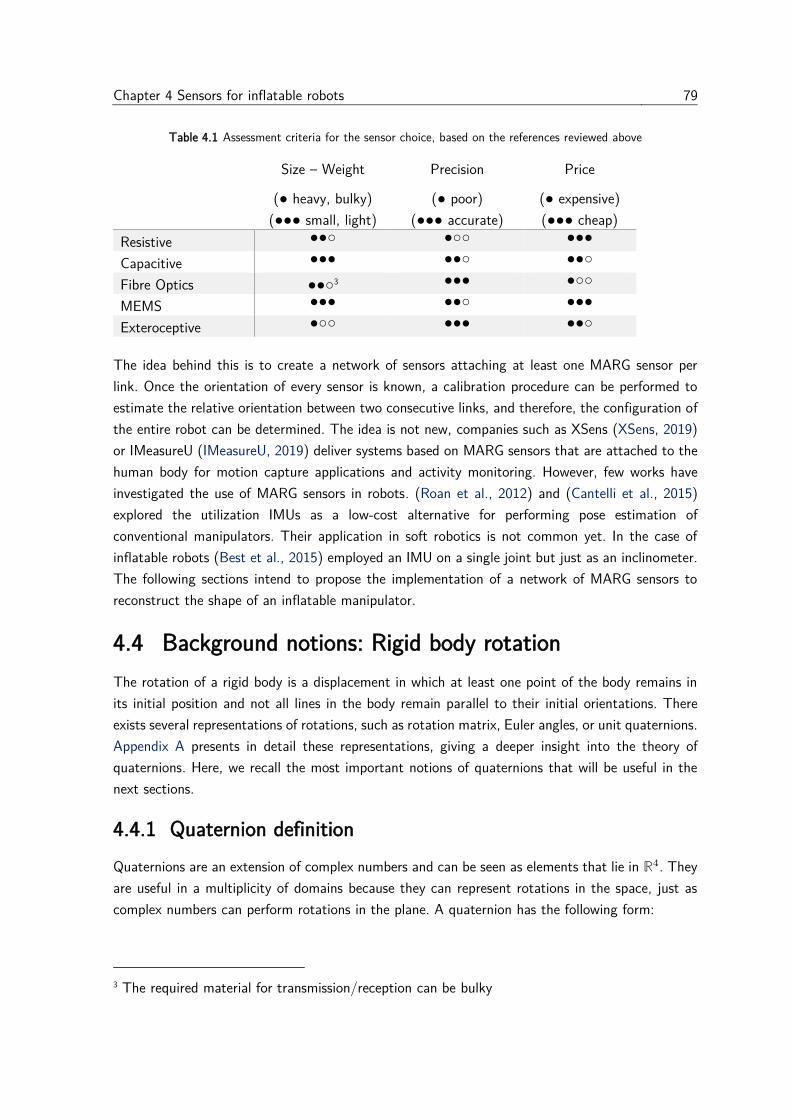
Chapter 4 Sensors for inflatable robots 79

Table 4.1 Assessment criteria for the sensor choice, based on the references reviewed above

Size – Weight

(● heavy, bulky)

(●●● small, light)

Precision

(● poor)

(●●● accurate)

Price

(● expensive)

(●●● cheap)

Resistive ●●○ ●○○ ●●●

Capacitive ●●● ●●○ ●●○

Fibre Optics ●●○3 ●●● ●○○

MEMS ●●● ●●○ ●●●

Exteroceptive ●○○ ●●● ●●○

The idea behind this is to create a network of sensors attaching at least one MARG sensor per

link. Once the orientation of every sensor is known, a calibration procedure can be performed to

estimate the relative orientation between two consecutive links, and therefore, the configuration of

the entire robot can be determined. The idea is not new, companies such as XSens (XSens, 2019)

or IMeasureU (IMeasureU, 2019) deliver systems based on MARG sensors that are attached to the

human body for motion capture applications and activity monitoring. However, few works have

investigated the use of MARG sensors in robots. (Roan et al., 2012) and (Cantelli et al., 2015)

explored the utilization IMUs as a low-cost alternative for performing pose estimation of

conventional manipulators. Their application in soft robotics is not common yet. In the case of

inflatable robots (Best et al., 2015) employed an IMU on a single joint but just as an inclinometer.

The following sections intend to propose the implementation of a network of MARG sensors to

reconstruct the shape of an inflatable manipulator.

4.4 Background notions: Rigid body rotation

The rotation of a rigid body is a displacement in which at least one point of the body remains in

its initial position and not all lines in the body remain parallel to their initial orientations. There

exists several representations of rotations, such as rotation matrix, Euler angles, or unit quaternions.

Appendix A presents in detail these representations, giving a deeper insight into the theory of

quaternions. Here, we recall the most important notions of quaternions that will be useful in the

next sections.

4.4.1 Quaternion definition

Quaternions are an extension of complex numbers and can be seen as elements that lie in ℝ4. They

are useful in a multiplicity of domains because they can represent rotations in the space, just as

complex numbers can perform rotations in the plane. A quaternion has the following form:

3 The required material for transmission/reception can be bulky

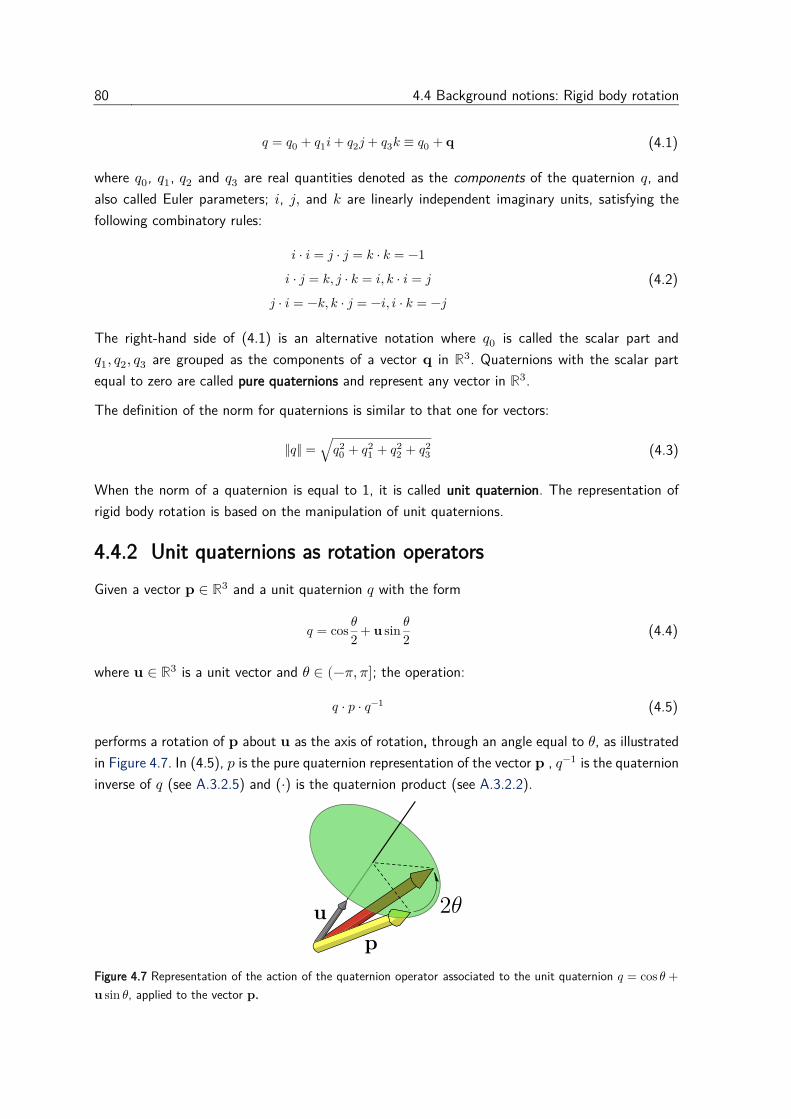
80 4.4 Background notions: Rigid body rotation

𝑞 = 𝑞0 + 𝑞1𝑖 + 𝑞2𝑗 + 𝑞3𝑘 ≡ 𝑞0 + 𝐪 (4.1)

where 𝑞0, 𝑞1, 𝑞2 and 𝑞3 are real quantities denoted as the components of the quaternion 𝑞, and

also called Euler parameters; 𝑖, 𝑗, and 𝑘 are linearly independent imaginary units, satisfying the

following combinatory rules:

𝑖 ⋅ 𝑖 = 𝑗 ⋅ 𝑗 = 𝑘 ⋅ 𝑘 = −1

𝑖 ⋅ 𝑗 = 𝑘, 𝑗 ⋅ 𝑘 = 𝑖, 𝑘 ⋅ 𝑖 = 𝑗

𝑗 ⋅ 𝑖 = −𝑘, 𝑘 ⋅ 𝑗 = −𝑖, 𝑖 ⋅ 𝑘 = −𝑗

(4.2)

The right-hand side of (4.1) is an alternative notation where 𝑞0 is called the scalar part and

𝑞1, 𝑞2, 𝑞3 are grouped as the components of a vector 𝐪 in ℝ3. Quaternions with the scalar part

equal to zero are called pure quaternions and represent any vector in ℝ3.

The definition of the norm for quaternions is similar to that one for vectors:

‖𝑞‖ = √𝑞02 + 𝑞1

2 + 𝑞22 + 𝑞3

2 (4.3)

When the norm of a quaternion is equal to 1, it is called unit quaternion. The representation of

rigid body rotation is based on the manipulation of unit quaternions.

4.4.2 Unit quaternions as rotation operators

Given a vector 𝐩 ∈ ℝ3 and a unit quaternion 𝑞 with the form

𝑞 = cos𝜃

2+ 𝐮 sin

𝜃

2 (4.4)

where 𝐮 ∈ ℝ3 is a unit vector and 𝜃 ∈ (−𝜋, 𝜋]; the operation:

𝑞 ⋅ 𝑝 ⋅ 𝑞−1 (4.5)

performs a rotation of 𝐩 about 𝐮 as the axis of rotation, through an angle equal to 𝜃, as illustrated

in Figure 4.7. In (4.5), 𝑝 is the pure quaternion representation of the vector 𝐩 , 𝑞−1 is the quaternion

inverse of 𝑞 (see A.3.2.5) and (⋅) is the quaternion product (see A.3.2.2).

Figure 4.7 Representation of the action of the quaternion operator associated to the unit quaternion 𝑞 = cos 𝜃 +

𝐮 sin 𝜃, applied to the vector 𝐩.

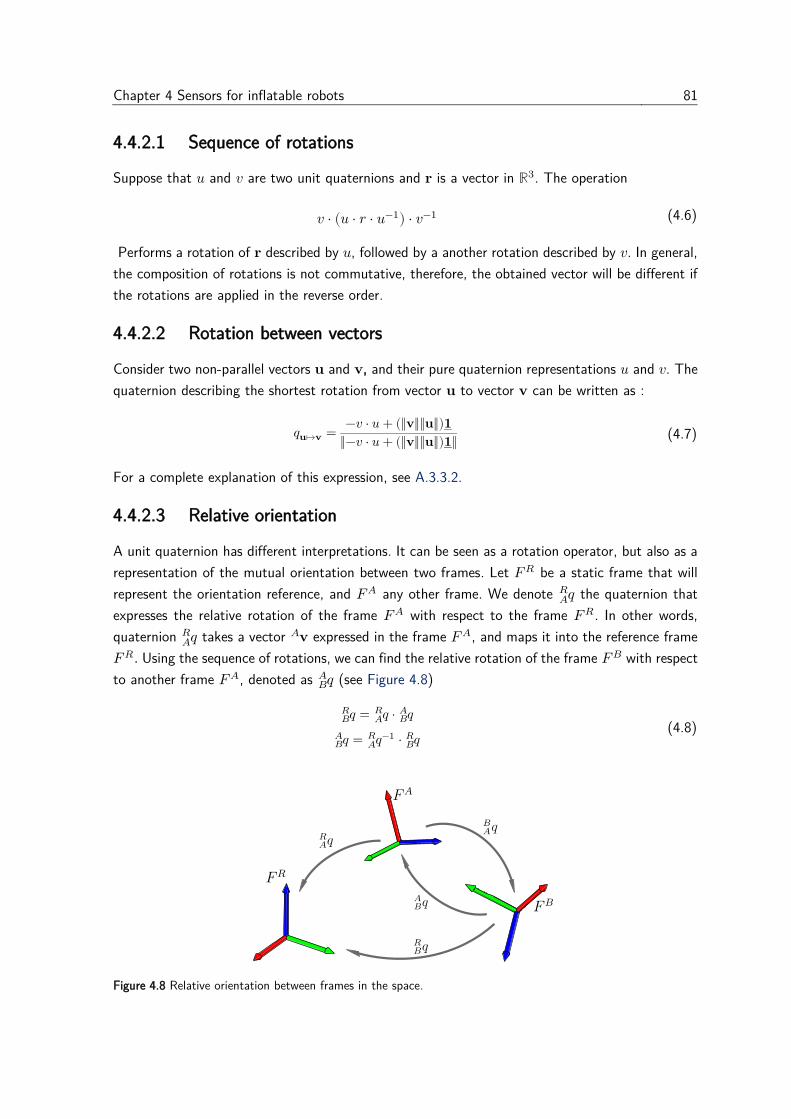
Chapter 4 Sensors for inflatable robots 81

4.4.2.1 Sequence of rotations

Suppose that 𝑢 and 𝑣 are two unit quaternions and 𝐫 is a vector in ℝ3. The operation

𝑣 ⋅ (𝑢 ⋅ 𝑟 ⋅ 𝑢−1) ⋅ 𝑣−1 (4.6)

Performs a rotation of 𝐫 described by 𝑢, followed by a another rotation described by 𝑣. In general,

the composition of rotations is not commutative, therefore, the obtained vector will be different if

the rotations are applied in the reverse order.

4.4.2.2 Rotation between vectors

Consider two non-parallel vectors 𝐮 and 𝐯, and their pure quaternion representations 𝑢 and 𝑣. The

quaternion describing the shortest rotation from vector 𝐮 to vector 𝐯 can be written as :

𝑞𝐮↦𝐯 =−𝑣 ⋅ 𝑢 + (‖𝐯‖‖𝐮‖)𝟏

‖−𝑣 ⋅ 𝑢 + (‖𝐯‖‖𝐮‖)𝟏‖ (4.7)

For a complete explanation of this expression, see A.3.3.2.

4.4.2.3 Relative orientation

A unit quaternion has different interpretations. It can be seen as a rotation operator, but also as a

representation of the mutual orientation between two frames. Let 𝐹𝑅 be a static frame that will

represent the orientation reference, and 𝐹𝐴 any other frame. We denote 𝑞𝐴𝑅 the quaternion that

expresses the relative rotation of the frame 𝐹𝐴 with respect to the frame 𝐹𝑅. In other words,

quaternion 𝑞𝐴𝑅 takes a vector 𝐯

𝐴 expressed in the frame 𝐹𝐴, and maps it into the reference frame

𝐹𝑅. Using the sequence of rotations, we can find the relative rotation of the frame 𝐹𝐵 with respect

to another frame 𝐹𝐴, denoted as 𝑞𝐵𝐴 (see Figure 4.8)

𝑞𝐵𝑅 = 𝑞𝐴

𝑅 ⋅ 𝑞𝐵𝐴

𝑞𝐵𝐴 = 𝑞𝐴

𝑅 −1 ⋅ 𝑞𝐵𝑅

(4.8)

Figure 4.8 Relative orientation between frames in the space.

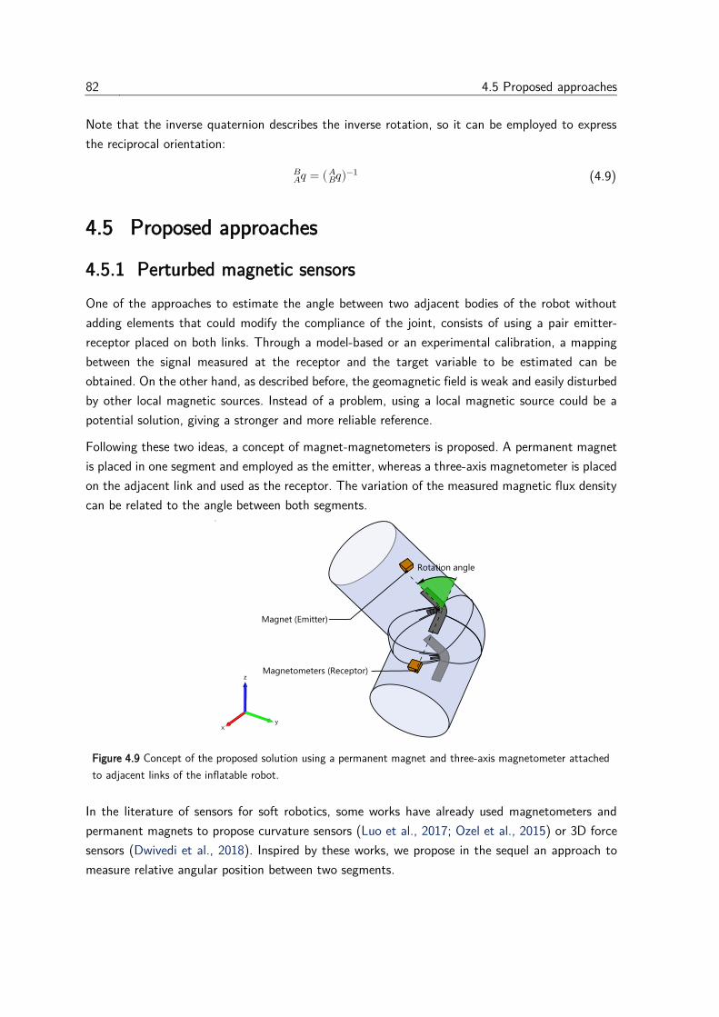
82 4.5 Proposed approaches

Note that the inverse quaternion describes the inverse rotation, so it can be employed to express

the reciprocal orientation:

𝑞𝐴𝐵 = ( 𝑞𝐵

𝐴 )−1 (4.9)

4.5 Proposed approaches

4.5.1 Perturbed magnetic sensors

One of the approaches to estimate the angle between two adjacent bodies of the robot without

adding elements that could modify the compliance of the joint, consists of using a pair emitter-

receptor placed on both links. Through a model-based or an experimental calibration, a mapping

between the signal measured at the receptor and the target variable to be estimated can be

obtained. On the other hand, as described before, the geomagnetic field is weak and easily disturbed

by other local magnetic sources. Instead of a problem, using a local magnetic source could be a

potential solution, giving a stronger and more reliable reference.

Following these two ideas, a concept of magnet-magnetometers is proposed. A permanent magnet

is placed in one segment and employed as the emitter, whereas a three-axis magnetometer is placed

on the adjacent link and used as the receptor. The variation of the measured magnetic flux density

can be related to the angle between both segments.

Figure 4.9 Concept of the proposed solution using a permanent magnet and three-axis magnetometer attached

to adjacent links of the inflatable robot.

In the literature of sensors for soft robotics, some works have already used magnetometers and

permanent magnets to propose curvature sensors (Luo et al., 2017; Ozel et al., 2015) or 3D force

sensors (Dwivedi et al., 2018). Inspired by these works, we propose in the sequel an approach to

measure relative angular position between two segments.

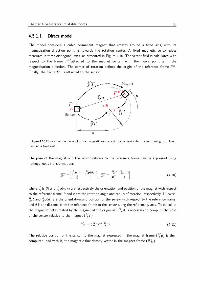
Chapter 4 Sensors for inflatable robots 83

4.5.1.1 Direct model

The model considers a cubic permanent magnet that rotates around a fixed axis, with its

magnetization direction pointing towards the rotation center. A fixed magnetic sensor gives

measures in three orthogonal axes, as presented in Figure 4.10. The vector field is calculated with

respect to the frame 𝐹𝑀attached to the magnet center, with the 𝑧-axis pointing in the

magnetization direction. The center of rotation defines the origin of the reference frame 𝐹𝑅.

Finally, the frame 𝐹𝑆 is attached to the sensor.

Figure 4.10 Diagram of the model of a fixed magnetic sensor and a permanent cubic magnet turning in a plane

around a fixed axis.

The pose of the magnet and the sensor relative to the reference frame can be expressed using

homogeneous transformations:

𝑇𝑀𝑅 = [

𝑅𝑀𝑅 (𝜃) 𝐩𝑀

𝑅 (𝜃, 𝑟)

𝟎3⊺ 1

] 𝑇𝑆𝑅 = [

𝑅𝑆𝑅 𝐩𝑆

𝑅 (𝑑)

𝟎3⊺ 1

] (4.10)

where 𝑅𝑀𝑅 (𝜃) and 𝐩𝑀

𝑅 (𝜃, 𝑟) are respectively the orientation and position of the magnet with respect

to the reference frame, 𝜃 and 𝑟 are the rotation angle and radius of rotation, respectively. Likewise,

𝑅𝑆𝑅 and 𝐩𝑆

𝑅 (𝑑) are the orientation and position of the sensor with respect to the reference frame,

and 𝑑 is the distance from the reference frame to the sensor along the reference 𝑦-axis. To calculate

the magnetic field created by the magnet at the origin of 𝐹𝑆, it is necessary to compute the pose

of the sensor relative to the magnet ( 𝑇𝑆𝑀 ):

𝑇𝑆𝑀 = ( 𝑇𝑀

𝑅 )−1( 𝑇𝑆𝑅 ) (4.11)

The relative position of the sensor to the magnet expressed in the magnet frame ( 𝐩𝑆𝑀 ) is then

computed, and with it, the magnetic flux density vector in the magnet frame (𝐁𝑀𝑆 ).

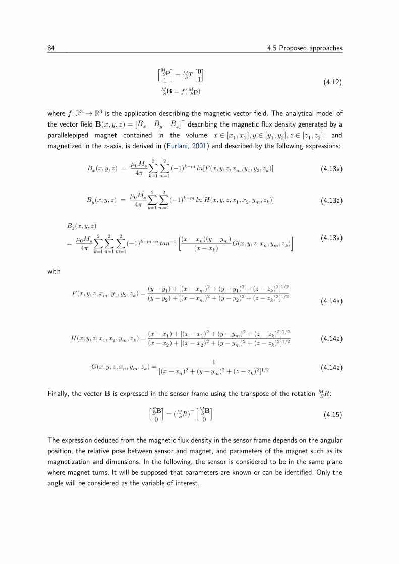
84 4.5 Proposed approaches

[ 𝐩𝑆𝑀

1] = 𝑇𝑆

𝑀 [𝟎1]

𝐁𝑆𝑀 = 𝑓( 𝐩𝑆

𝑀 )

(4.12)

where 𝑓: ℝ3 → ℝ3 is the application describing the magnetic vector field. The analytical model of

the vector field 𝐁(𝑥, 𝑦, 𝑧) = [𝐵𝑥 𝐵𝑦 𝐵𝑧]⊺ describing the magnetic flux density generated by a

parallelepiped magnet contained in the volume 𝑥 ∈ [𝑥1, 𝑥2], 𝑦 ∈ [𝑦1, 𝑦2], 𝑧 ∈ [𝑧1, 𝑧2], and

magnetized in the 𝑧-axis, is derived in (Furlani, 2001) and described by the following expressions:

𝐵𝑥(𝑥, 𝑦, 𝑧) = 𝜇0𝑀𝑠4𝜋∑∑(−1)𝑘+𝑚 𝑙𝑛[𝐹 (𝑥, 𝑦, 𝑧, 𝑥𝑚, 𝑦1, 𝑦2, 𝑧𝑘)]

2

𝑚=1

2

𝑘=1

(4.13a)

𝐵𝑦(𝑥, 𝑦, 𝑧) = 𝜇0𝑀𝑠4𝜋∑∑(−1)𝑘+𝑚 𝑙𝑛[𝐻(𝑥, 𝑦, 𝑧, 𝑥1, 𝑥2, 𝑦𝑚, 𝑧𝑘)]

2

𝑚=1

2

𝑘=1

(4.13a)

𝐵𝑧(𝑥, 𝑦, 𝑧)

= 𝜇0𝑀𝑠4𝜋∑∑∑(−1)𝑘+𝑚+𝑛 𝑡𝑎𝑛−1 [

(𝑥 − 𝑥𝑛)(𝑦 − 𝑦𝑚)

(𝑥 − 𝑥𝑘)𝐺(𝑥, 𝑦, 𝑧, 𝑥𝑛, 𝑦𝑚, 𝑧𝑘)]

2

𝑚=1

2

𝑛=1

2

𝑘=1

(4.13a)

with

𝐹(𝑥, 𝑦, 𝑧, 𝑥𝑚, 𝑦1, 𝑦2, 𝑧𝑘) =(𝑦 − 𝑦1) + [(𝑥 − 𝑥𝑚)

2 + (𝑦 − 𝑦1)2 + (𝑧 − 𝑧𝑘)

2]1 2⁄

(𝑦 − 𝑦2) + [(𝑥 − 𝑥𝑚)2 + (𝑦 − 𝑦2)

2 + (𝑧 − 𝑧𝑘)2]1 2⁄

(4.14a)

𝐻(𝑥, 𝑦, 𝑧, 𝑥1, 𝑥2, 𝑦𝑚, 𝑧𝑘) =(𝑥 − 𝑥1) + [(𝑥 − 𝑥1)

2 + (𝑦 − 𝑦𝑚)2 + (𝑧 − 𝑧𝑘)

2]1 2⁄

(𝑥 − 𝑥2) + [(𝑥 − 𝑥2)2 + (𝑦 − 𝑦𝑚)

2 + (𝑧 − 𝑧𝑘)2]1 2⁄

(4.14a)

𝐺(𝑥, 𝑦, 𝑧, 𝑥𝑛, 𝑦𝑚, 𝑧𝑘) =1

[(𝑥 − 𝑥𝑛)2 + (𝑦 − 𝑦𝑚)

2 + (𝑧 − 𝑧𝑘)2]1 2⁄

(4.14a)

Finally, the vector 𝐁 is expressed in the sensor frame using the transpose of the rotation 𝑅𝑆𝑀 :

[ 𝐁𝐵𝑆

0] = ( 𝑅𝑆

𝑀 )⊺ [ 𝐁𝑆𝑀

0] (4.15)

The expression deduced from the magnetic flux density in the sensor frame depends on the angular

position, the relative pose between sensor and magnet, and parameters of the magnet such as its

magnetization and dimensions. In the following, the sensor is considered to be in the same plane

where magnet turns. It will be supposed that parameters are known or can be identified. Only the

angle will be considered as the variable of interest.

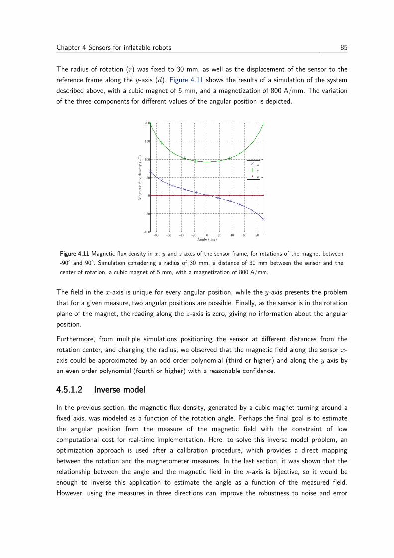
Chapter 4 Sensors for inflatable robots 85

The radius of rotation (𝑟) was fixed to 30 mm, as well as the displacement of the sensor to the

reference frame along the 𝑦-axis (𝑑). Figure 4.11 shows the results of a simulation of the system

described above, with a cubic magnet of 5 mm, and a magnetization of 800 A/mm. The variation

of the three components for different values of the angular position is depicted.

Figure 4.11 Magnetic flux density in 𝑥, 𝑦 and 𝑧 axes of the sensor frame, for rotations of the magnet between

-90° and 90°. Simulation considering a radius of 30 mm, a distance of 30 mm between the sensor and the

center of rotation, a cubic magnet of 5 mm, with a magnetization of 800 A/mm.

The field in the 𝑥-axis is unique for every angular position, while the 𝑦-axis presents the problem

that for a given measure, two angular positions are possible. Finally, as the sensor is in the rotation

plane of the magnet, the reading along the 𝑧-axis is zero, giving no information about the angular

position.

Furthermore, from multiple simulations positioning the sensor at different distances from the

rotation center, and changing the radius, we observed that the magnetic field along the sensor 𝑥-

axis could be approximated by an odd order polynomial (third or higher) and along the 𝑦-axis by

an even order polynomial (fourth or higher) with a reasonable confidence.

4.5.1.2 Inverse model

In the previous section, the magnetic flux density, generated by a cubic magnet turning around a

fixed axis, was modeled as a function of the rotation angle. Perhaps the final goal is to estimate

the angular position from the measure of the magnetic field with the constraint of low

computational cost for real-time implementation. Here, to solve this inverse model problem, an

optimization approach is used after a calibration procedure, which provides a direct mapping

between the rotation and the magnetometer measures. In the last section, it was shown that the

relationship between the angle and the magnetic field in the x-axis is bijective, so it would be

enough to inverse this application to estimate the angle as a function of the measured field.

However, using the measures in three directions can improve the robustness to noise and error

86 4.5 Proposed approaches

model, as it will be shown in section 4.5.1.3. Thus, three polynomials can be obtained, relating the

magnetic field in every direction with the angle:

�̂�(𝜃) = [�̂�𝑥(𝜃) �̂�𝑦(𝜃) �̂�𝑧(𝜃)]⊺ (4.16)

To estimate the angle from a measure of the magnetic field in three directions, a set of three

nonlinear equations with only one unknown, i.e., the angle, must be solved. To solve this over-

constrained problem, a gradient descent method is employed. The cost function to be minimized

is the following mean squared relative error

1

3∑ (

𝐵𝑖𝑚𝑒𝑎𝑠 − �̂�𝑖(𝜃)

𝐵𝑖𝑟𝑎𝑛𝑔𝑒 )

2

𝑖 ∈ {𝑥,𝑦,𝑧}

(4.17)

where 𝐵𝑖𝑚𝑒𝑎𝑠 are the vector components of the measured magnetic field, and 𝐵𝑖

𝑟𝑎𝑛𝑔𝑒 is the range

of measures along the axis 𝑖, obtained during the calibration procedure. To initialize the algorithm

at the time step 𝑘, a good guess is the estimation computed at time step 𝑘 − 1, supposing that

there are not abrupt changes in the angular position. For the first time step 𝑘 = 0, the root of the

equation �̂�𝑥 −𝐵𝑥𝑚𝑒𝑎𝑠 = 0 constitutes a good initial guess.

4.5.1.3 Experimental Results

Test in a mockup

To validate the model described in section III, a simple mockup was constructed with non-

ferromagnetic materials, namely wood and plastic (see Figure 4.12). The employed sensor was a

Bosch BNO055, with three orthogonal magnetometers. The measurement range along the local x

and y axis is ±1300 µT (13 bits resolution) and along z axis ±2500 µT (15 bits resolution). The

sample rate was fixed to 30 Hz, the maximal sample rate of the magnetometers. The sensor was

connected to an Arduino Zero board by I2C bus. The angular position was measured with a

potentiometer, using an AD converter of 10 bits of resolution. The magnet utilized was a 5 mm

neodymium cube, with a magnetization of 800 A/mm approximately.

Figure 4.12 Mock-up constructed to validate the model. The three-axis magnetometer is oriented as shown by

axes 𝑥 and 𝑦. Parameters 𝑑 and 𝑟 correspond to the distance to the center of rotation and the radius, as defined

previously in the diagram of Figure 4.10.

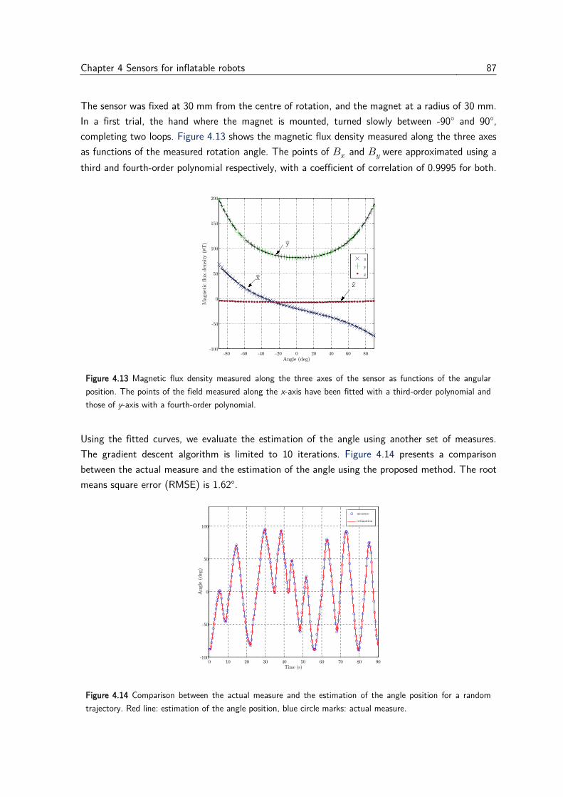
Chapter 4 Sensors for inflatable robots 87

The sensor was fixed at 30 mm from the centre of rotation, and the magnet at a radius of 30 mm.

In a first trial, the hand where the magnet is mounted, turned slowly between -90° and 90°,

completing two loops. Figure 4.13 shows the magnetic flux density measured along the three axes

as functions of the measured rotation angle. The points of 𝐵𝑥 and 𝐵𝑦 were approximated using a

third and fourth-order polynomial respectively, with a coefficient of correlation of 0.9995 for both.

Figure 4.13 Magnetic flux density measured along the three axes of the sensor as functions of the angular

position. The points of the field measured along the x-axis have been fitted with a third-order polynomial and

those of y-axis with a fourth-order polynomial.

Using the fitted curves, we evaluate the estimation of the angle using another set of measures.

The gradient descent algorithm is limited to 10 iterations. Figure 4.14 presents a comparison

between the actual measure and the estimation of the angle using the proposed method. The root

means square error (RMSE) is 1.62°.

Figure 4.14 Comparison between the actual measure and the estimation of the angle position for a random

trajectory. Red line: estimation of the angle position, blue circle marks: actual measure.

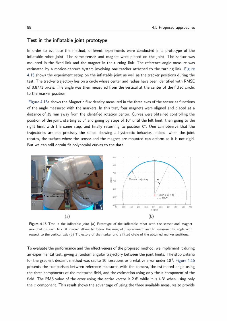
88 4.5 Proposed approaches

Test in the inflatable joint prototype

In order to evaluate the method, different experiments were conducted in a prototype of the

inflatable robot joint. The same sensor and magnet were placed on the joint. The sensor was

mounted in the fixed link and the magnet in the turning link. The reference angle measure was

estimated by a motion-capture system involving one tracker attached to the turning link. Figure

4.15 shows the experiment setup on the inflatable joint as well as the tracker positions during the

test. The tracker trajectory lies on a circle whose center and radius have been identified with RMSE

of 0.8773 pixels. The angle was then measured from the vertical at the center of the fitted circle,

to the marker position.

Figure 4.16a shows the Magnetic flux density measured in the three axes of the sensor as functions

of the angle measured with the markers. In this test, four magnets were aligned and placed at a

distance of 35 mm away from the identified rotation center. Curves were obtained controlling the

position of the joint, starting at 0° and going by steps of 10° until the left limit, then going to the

right limit with the same step, and finally returning to position 0°. One can observe that the

trajectories are not precisely the same, showing a hysteretic behavior. Indeed, when the joint

rotates, the surface where the sensor and the magnet are mounted can deform as it is not rigid.

But we can still obtain fit polynomial curves to the data.

(a) (b)

Figure 4.15 Test in the inflatable joint (a) Prototype of the inflatable robot with the sensor and magnet

mounted on each link. A marker allows to follow the magnet displacement and to measure the angle with

respect to the vertical axis (b) Trajectory of the marker and a fitted circle of the obtained marker positions.

To evaluate the performance and the effectiveness of the proposed method, we implement it during

an experimental test, giving a random angular trajectory between the joint limits. The stop criteria

for the gradient descent method was set to 10 iterations or a relative error under 10-3. Figure 4.16

presents the comparison between reference measured with the camera, the estimated angle using

the three components of the measured field, and the estimation using only the 𝑥 component of the

field. The RMS value of the error using the entire vector is 2.6° while it is 4.3° when using only

the 𝑥 component. This result shows the advantage of using the three available measures to provide

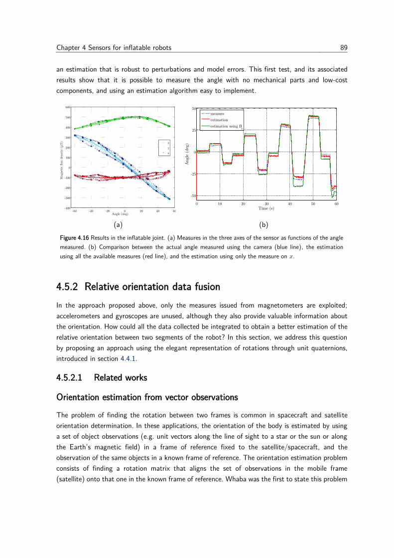
Chapter 4 Sensors for inflatable robots 89

an estimation that is robust to perturbations and model errors. This first test, and its associated

results show that it is possible to measure the angle with no mechanical parts and low-cost

components, and using an estimation algorithm easy to implement.

(a) (b)

Figure 4.16 Results in the inflatable joint. (a) Measures in the three axes of the sensor as functions of the angle

measured. (b) Comparison between the actual angle measured using the camera (blue line), the estimation

using all the available measures (red line), and the estimation using only the measure on 𝑥.

4.5.2 Relative orientation data fusion

In the approach proposed above, only the measures issued from magnetometers are exploited;

accelerometers and gyroscopes are unused, although they also provide valuable information about

the orientation. How could all the data collected be integrated to obtain a better estimation of the

relative orientation between two segments of the robot? In this section, we address this question

by proposing an approach using the elegant representation of rotations through unit quaternions,

introduced in section 4.4.1.

4.5.2.1 Related works

Orientation estimation from vector observations

The problem of finding the rotation between two frames is common in spacecraft and satellite

orientation determination. In these applications, the orientation of the body is estimated by using

a set of object observations (e.g. unit vectors along the line of sight to a star or the sun or along

the Earth’s magnetic field) in a frame of reference fixed to the satellite/spacecraft, and the

observation of the same objects in a known frame of reference. The orientation estimation problem

consists of finding a rotation matrix that aligns the set of observations in the mobile frame

(satellite) onto that one in the known frame of reference. Whaba was the first to state this problem

90 4.5 Proposed approaches

(Wahba, 1965), seeking for an optimal orthogonal matrix that minimizes a least square loss

function using 𝑛 (𝑛 ≥ 2) unit vector pairs:

𝑀 = argmin∑ ‖𝐯𝑖∗ −𝑀𝐯𝑖‖

2𝑛

𝑖=1

Where 𝐯𝑖∗ is the object observation 𝑖 in the mobile frame, and 𝐯𝑖 is the observation of the same

object in the reference frame. Since then, several algorithms have been proposed, classified into

two approaches (Wertz, 1978):

Deterministic methods consider a minimal set of observations (two pairs) and find a closed solution

by solving a set of non-linear equations. They often guarantee a solution and require minimal a

priori information to give an estimation. Therefore, they are commonly used to compute an initial

estimation. However, as they use minimal information, they have low immunity to noise. Some of

the existing algorithms are TRIAD (Lerner, 1978), Euler-2 (Mortari, 1995) or the algorithm

proposed by (Horn, 1987).

Optimal methods consider more than two observations, they can combine larger quantities of data

to compute an optimal estimate based on the minimization of a cost function, as proposed by

Wahba. Multiple optimization algorithms have been proposed, using quaternions such as the q-

method (Keat, 1977), QUEST (Quaternion Estimator) (Shuster and Oh, 1981), FOAM (Fast

Optimal Matrix Algorithm) (Markley, 1988) or Euler-n (Mortari, 1995).

State estimation methods are a particular subset of optimal methods correct estimates successively.

In contrast with deterministic methods, state estimation approaches can diverge, need an accurate

initialization, and the results are not always easy to interpret. However, these methods can provide

statistically optimal solutions and combine data from different sources.

Actually, both methods are employed in a complementary fashion. As deterministic methods require

minimal a priori information, they are commonly used to compute an initial estimation that is then

employed by a state estimation method. State estimation outputs can be compared to deterministic

methods to ensure that the solution has not diverged.

In orientation estimation using MARG (Magnetic, Angle Rate, and Gravity) sensors, only a set of

two vectors is considered: one pointing in the direction of the gravity, and another one, pointing

towards the magnetic field of the earth. Hence, the accelerometer gives information about the

inclination, while the magnetometer provides information about the heading. As it represents the

case of a minimal set of observations, the utilization of deterministic algorithms is more appropriate

than optimization approaches that can be slow to converge.

A common approach to pose estimation using the gravitational and magnetic fields as observation

vectors decomposes the problem in two parts: first, find the rotation that aligns the accelerometer

observation with the gravity reference vector. Then, align the rotated magnetometer measure to

its reference, while keeping aligned the accelerometer observation to its reference. This method

ensures a decoupled effect of disturbances in the estimation: if the magnetometer is disturbed, the

Chapter 4 Sensors for inflatable robots 91

influence will affect only the estimated rotation in a horizontal plane, and the inclination estimation

will remain untouched. Based on this approach, (Madgwick et al., 2011) proposed a complementary

filter between a quaternion estimation obtained from the integration of gyroscope measures, and a

second estimation obtained from accelerometer and magnetometer measures using a gradient

descent approach. (Valenti et al., 2015) proposed an algebraic exact solution of the same decoupled

problem, provided that the vector set in the reference frame is relatively simple (the reference

vector of gravity points in the 𝑧 direction and magnetic field lies on the 𝑥𝑧 plane), so the system

of non-linear equations is reduced to simpler expressions that can be solved analytically.

In this work, we propose an extension of this approach, considering any minimal set of non-collinear

vectors. This will be the basis to develop an estimator of the relative orientation between two

frames, which considers that both of them are mobile and the vector observations in every frame

will variate over time.

4.5.2.2 Problem formulation

Let 𝐹 1 and 𝐹 2 be two different frames in the space, whose relative orientation is required to be

estimated, denoted by the unit quaternion 𝑞21 . On the other hand, 𝐠 and 𝐦 are two unit vectors,

non-collinear and static with respect to an inertial frame. The observations of 𝐠 from frames 𝐹 1

and 𝐹 2 are denoted 𝐠 1 and 𝐠

2 respectively. Likewise, 𝐦 1 and 𝐦

2 denote the vector observations

of 𝐦 in both frames. Note that the exact directions of 𝐠 and 𝐦 are not required; the only

requirement is that both sets of observations correspond to the same vectors. The problem of

relative orientation consists to find a rotation that aligns the vector observations 𝐠 2 and 𝐦

2 into

𝐠 1 and 𝐦

1 .

In the particular studied case, vectors 𝐠 and 𝐦 represent the direction of gravity and earth magnetic

field, and 𝐹 1 and 𝐹 2 are frames attached to two adjacent bodies in a serial manipulator. In this

case, the requirement that both sets of observations correspond to the same vectors is not always

guaranteed. For instance, the magnetic field can be easily perturbed locally, and the measure in

one of the frames will not correspond to the same vector as measured in the other frame. In the

case of accelerometer measures, if one of the frames suffers an acceleration, the measure will be

the vector sum of the gravity and the applied acceleration, giving a false observation of the

reference vector. But if we suppose that both frames are accelerated in a similar fashion or

perturbed uniformly by an external magnetic field, as it could happen in two adjacent bodies of a

serial manipulator, the resulting observations will be close to the same vector.

4.5.2.3 Proposed solution

Following the approach presented before, a first rotation must align the observed gravity vector in

frame 𝐹 2 to the one observed in 𝐹 1, namely 𝐠 2 to 𝐠

1 . Applying the expression for the rotation

between vectors presented in (4.7), the unit quaternion that aligns both vectors is given by:

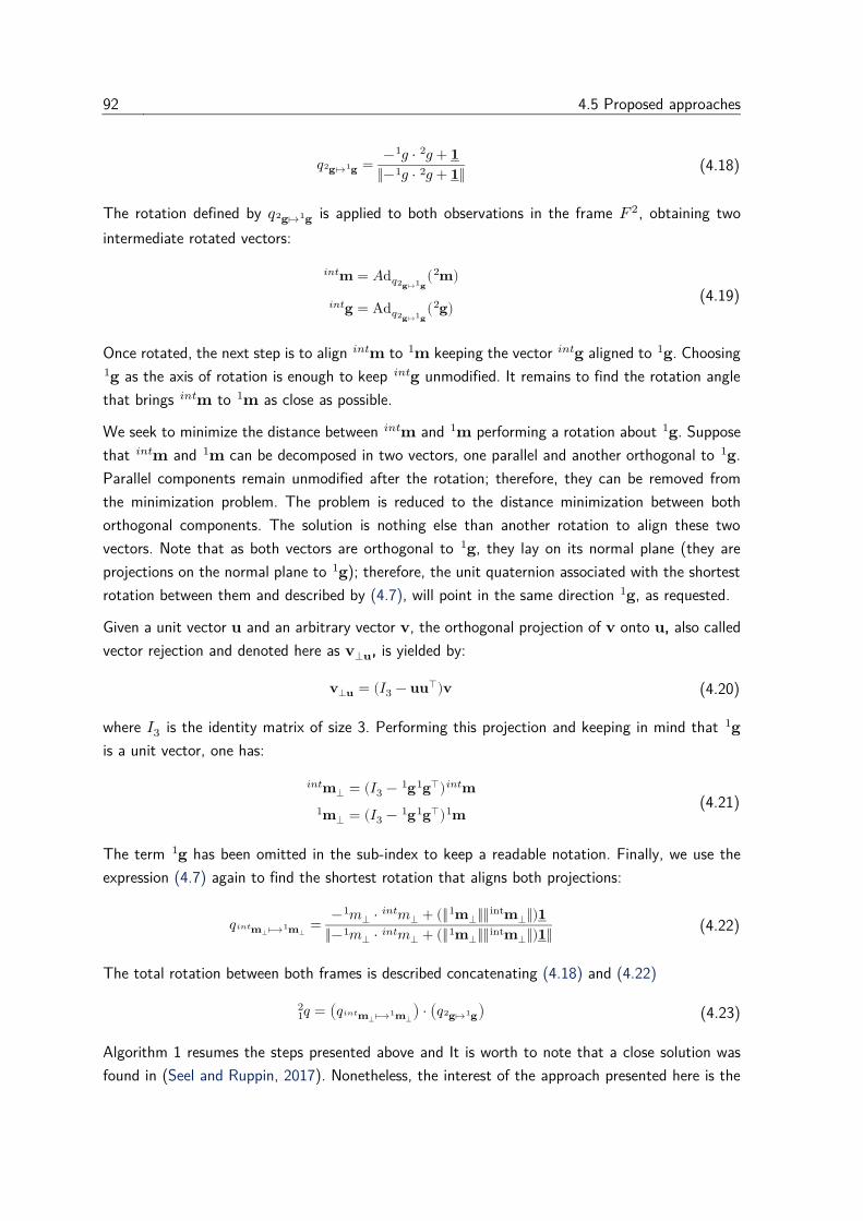
92 4.5 Proposed approaches

𝑞 𝐠 2 ↦ 𝐠 1 =− 𝑔 1 ⋅ 𝑔

2 + 𝟏

‖− 𝑔 1 ⋅ 𝑔

2 + 𝟏‖ (4.18)

The rotation defined by 𝑞 𝐠 2 ↦ 𝐠 1 is applied to both observations in the frame 𝐹 2, obtaining two

intermediate rotated vectors:

𝐦 𝑖𝑛𝑡 = 𝐴d𝑞

𝐠 2 ↦ 𝐠

1( 𝐦 2 )

𝐠 𝑖𝑛𝑡 = Ad𝑞

𝐠 2 ↦ 𝐠

1( 𝐠 2 )

(4.19)

Once rotated, the next step is to align 𝐦 𝑖𝑛𝑡 to 𝐦

1 keeping the vector 𝐠 𝑖𝑛𝑡 aligned to 𝐠

1 . Choosing

𝐠 1 as the axis of rotation is enough to keep 𝐠

𝑖𝑛𝑡 unmodified. It remains to find the rotation angle

that brings 𝐦 𝑖𝑛𝑡 to 𝐦

1 as close as possible.

We seek to minimize the distance between 𝐦 𝑖𝑛𝑡 and 𝐦

1 performing a rotation about 𝐠 1 . Suppose

that 𝐦 𝑖𝑛𝑡 and 𝐦

1 can be decomposed in two vectors, one parallel and another orthogonal to 𝐠 1 .

Parallel components remain unmodified after the rotation; therefore, they can be removed from

the minimization problem. The problem is reduced to the distance minimization between both

orthogonal components. The solution is nothing else than another rotation to align these two

vectors. Note that as both vectors are orthogonal to 𝐠 1 , they lay on its normal plane (they are

projections on the normal plane to 𝐠 1 ); therefore, the unit quaternion associated with the shortest

rotation between them and described by (4.7), will point in the same direction 𝐠 1 , as requested.

Given a unit vector 𝐮 and an arbitrary vector 𝐯, the orthogonal projection of 𝐯 onto 𝐮, also called

vector rejection and denoted here as 𝐯⊥𝐮, is yielded by:

𝐯⊥𝐮 = (𝐼3 − 𝐮𝐮⊺)𝐯 (4.20)

where 𝐼3 is the identity matrix of size 3. Performing this projection and keeping in mind that 𝐠 1

is a unit vector, one has:

𝐦⊥ 𝑖𝑛𝑡 = (𝐼3 − 𝐠

1 𝐠 1 ⊺) 𝐦

𝑖𝑛𝑡

𝐦⊥ 1 = (𝐼3 − 𝐠

1 𝐠 1 ⊺) 𝐦

1 (4.21)

The term 𝐠 1 has been omitted in the sub-index to keep a readable notation. Finally, we use the

expression (4.7) again to find the shortest rotation that aligns both projections:

𝑞 𝐦⊥ 𝑖𝑛𝑡 ⟼ 𝐦⊥

1 =− 𝑚⊥ 1 ⋅ 𝑚⊥

𝑖𝑛𝑡 + (‖ 𝐦⊥ 1 ‖‖ 𝐦⊥

int ‖)𝟏

‖− 𝑚⊥ 1 ⋅ 𝑚⊥

𝑖𝑛𝑡 + (‖ 𝐦⊥ 1 ‖‖ 𝐦⊥

int ‖)𝟏‖ (4.22)

The total rotation between both frames is described concatenating (4.18) and (4.22)

𝑞12 = (𝑞 𝐦⊥

𝑖𝑛𝑡 ⟼ 𝐦⊥ 1 ) ⋅ (𝑞 𝐠 2 ↦ 𝐠 1 ) (4.23)

Algorithm 1 resumes the steps presented above and It is worth to note that a close solution was

found in (Seel and Ruppin, 2017). Nonetheless, the interest of the approach presented here is the

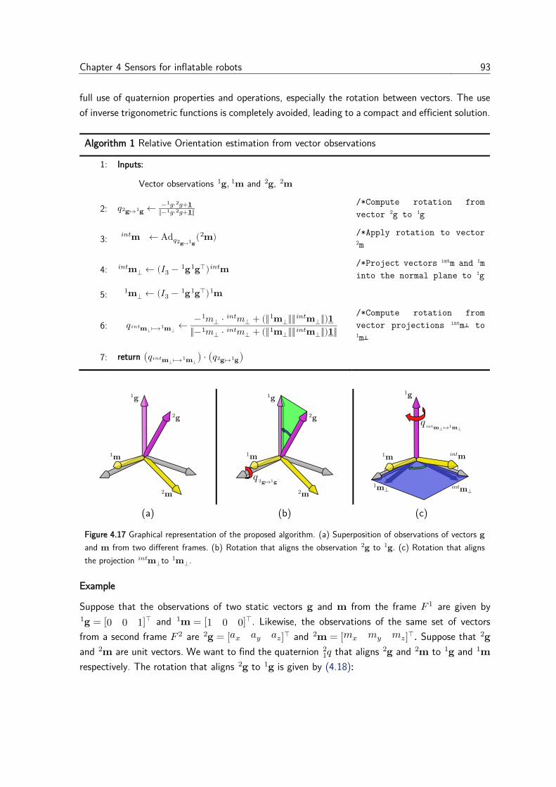
Chapter 4 Sensors for inflatable robots 93

full use of quaternion properties and operations, especially the rotation between vectors. The use

of inverse trigonometric functions is completely avoided, leading to a compact and efficient solution.

Algorithm 1 Relative Orientation estimation from vector observations

1: Inputs:

Vector observations 𝐠 1 , 𝐦

1 and 𝐠 2 , 𝐦

2

2: 𝑞 𝐠 2 ↦ 𝐠 1 ←− 𝑔 1 ⋅ 𝑔 2 +𝟏

‖− 𝑔 1 ⋅ 𝑔 2 +𝟏‖

/*Compute rotation from

vector 2g to 1g

3: 𝐦 𝑖𝑛𝑡 ← Ad𝑞

𝐠 2 ↦ 𝐠

1( 𝐦 2 ) /*Apply rotation to vector

2m

4: 𝐦⊥ 𝑖𝑛𝑡 ← (𝐼3 − 𝐠

1 𝐠 1 ⊺) 𝐦

𝑖𝑛𝑡 /*Project vectors intm and 1m

into the normal plane to 1g

5: 𝐦⊥ 1 ← (𝐼3 − 𝐠

1 𝐠 1 ⊺) 𝐦

1

6: 𝑞 𝐦⊥ 𝑖𝑛𝑡 ⟼ 𝐦⊥

1 ←− 𝑚⊥ 1 ⋅ 𝑚⊥

𝑖𝑛𝑡 + (‖ 𝐦⊥ 1 ‖‖ 𝐦⊥

𝑖𝑛𝑡 ‖)𝟏

‖− 𝑚⊥ 1 ⋅ 𝑚⊥

𝑖𝑛𝑡 + (‖ 𝐦⊥ 1 ‖‖ 𝐦⊥

𝑖𝑛𝑡 ‖)𝟏‖

/*Compute rotation from

vector projections intm┴ to 1m┴

7: return (𝑞 𝐦⊥ 𝑖𝑛𝑡 ⟼ 𝐦⊥

1 ) ⋅ (𝑞 𝐠 2 ↦ 𝐠 1 )

(a) (b) (c)

Figure 4.17 Graphical representation of the proposed algorithm. (a) Superposition of observations of vectors 𝐠

and 𝐦 from two different frames. (b) Rotation that aligns the observation 𝐠 2 to 𝐠

1 . (c) Rotation that aligns

the projection 𝐦 𝑖𝑛𝑡

⊥to 𝐦 1⊥.

Example

Suppose that the observations of two static vectors 𝐠 and 𝐦 from the frame 𝐹 1 are given by

𝐠 1 = [0 0 1]⊺ and 𝐦

1 = [1 0 0]⊺. Likewise, the observations of the same set of vectors

from a second frame 𝐹 2 are 𝐠 2 = [𝑎𝑥 𝑎𝑦 𝑎𝑧]⊺ and 𝐦

2 = [𝑚𝑥 𝑚𝑦 𝑚𝑧]⊺. Suppose that 𝐠 2

and 𝐦 2 are unit vectors. We want to find the quaternion 𝑞1

2 that aligns 𝐠 2 and 𝐦

2 to 𝐠 1 and 𝐦

1

respectively. The rotation that aligns 𝐠 2 to 𝐠

1 is given by (4.18):

94 4.5 Proposed approaches

𝑞 𝐠 2 ↦ 𝐠 1 =− 𝑔 1 ⋅ 𝑔

2 + 𝟏

‖− 𝑔 1 ⋅ 𝑔

2 + 𝟏‖=

1

√2(𝑎𝑧 + 1)[

𝑎𝑧 + 1𝑎𝑦−𝑎𝑥0 ]

(4.24)

There is a singularity at 𝑎𝑧 = −1. In this situation, vectors 𝐠 1 and 𝐠

2 point in opposite directions,

one pointing up and the other one pointing down. Therefore, the solution is not unique.

This rotation is applied to the magnetometer reading, obtaining an intermediate vector 𝐥:

𝐥 = Ad𝑞𝐠 2 ↦ 𝐠

1( 𝐦 2 ) = [𝑙𝑥 𝑙𝑦 𝑙𝑧]

⊺

The next step is to compute the projections of 𝐥 and 𝐦 1 onto the normal plane of 𝐠

1 . In this

particular case, 𝐦 1 is orthogonal to 𝐠

1 , therefore the vector and its projection are the same.

𝐥⊥ = (𝐼3 − 𝐠 1 𝐠 1 ⊺)𝐥 = [

1 0 00 1 00 0 0

]

[ 𝑙𝑥𝑙𝑦𝑙𝑧] =[ 𝑙𝑥𝑙𝑦0]

𝐦 1⊥ = 𝐦

1 = [1 0 0]⊺

We denote Γ = 𝑙𝑥2 + 𝑙𝑦

2 the square of the norm of the projection 𝐥⊥. The rotation that aligns 𝐥⊥ to

𝐦 1⊥ is described by:

𝑞𝐥⊥⟼ 𝐦⊥ 1 =

− 𝑚⊥ 1 ⋅ 𝑙⊥ + (‖ 𝐦⊥

1 ‖‖𝐥⊥‖)𝟏

‖− 𝑚⊥ 1 ⋅ 𝑙⊥ + (‖ 𝐦⊥

1 ‖‖𝐥⊥‖)𝟏‖=

1

√(𝑙𝑥 +√Γ)2+ 𝑙𝑦2

[

𝑙𝑥 +√Γ

00−𝑙𝑦 ]

After simplification,

𝑞𝐥⊥⟼ 𝐦⊥ 1 =

[ √𝑙𝑥 +

√𝛤

20 0

−𝑙𝑦

√2(𝛤 + 𝑙𝑥√𝛤)]

⊺

(4.25)

Note that the components 𝑞1 and 𝑞2 of the quaternion 𝑞𝐥⊥⟼ 𝐦⊥ 1 are zero, which means that it

performs a rotation around the 𝑧-axis, parallel to 𝐠 1 , as expected. Finally, both expressions (4.24)

and (4.25) are concatenated to obtain the total orientation. These expressions are similar to those

obtained in (Valenti et al., 2015).

Results

To test the effectiveness of the method, a simulation similar to the one presented in (Valenti et

al., 2015) was carried out. A mobile frame is aligned initially with the global frame, then, three

consecutive rotations of 2𝜋 radians are performed around the principal axes 𝑥, 𝑦 and 𝑧 at a rate

of 2𝜋/5 𝑟𝑎𝑑/𝑠. The absolute orientation of the mobile frame is measured with a perfect sensor.

The local acceleration and magnetic field observations are obtained by rotating the global

Chapter 4 Sensors for inflatable robots 95

normalised vectors of gravity and magnetic field. In order to show that the method does not require

that reference vectors lay on principal axes, the following vectors were used as reference:

𝐠 1 = (1

√3⁄ )[1 1 −1]⊺

𝐦 1 = (2

√5⁄ )[1 0 1 2⁄ ]⊺

Both of them are unit vectors but they are not orthogonal. The observations are introduced into

the estimator, and the output is finally compared with the perfect measure, as shown in Figure

4.18.

(a)

(b)

Figure 4.18 Validation of orientation estimation (a) Simulation performing three rotations of 2𝜋 radians around

principal axes 𝑥, 𝑦 and 𝑧. Solid lines are the components of the orientation obtained from the perfect sensor,

dashed lines are the components of the estimated orientation. (b) XYZ Euler angles of the orientation.

Note how the estimated quaternion follows the perfect measure when the component 𝑞0 is positive,

even if the reference vectors do not lay in principal axes nor are mutually orthogonal. When 𝑞0 hits

0, the vector components jump between positive and negative values. The reason is that the

estimation represents the shortest rotation, therefore the component 𝑞0 remains positive whereas

the vector components present discontinuities, indicating that the rotation axis alternates its

direction.

96 4.5 Proposed approaches

4.5.2.4 Derivative of the inverse quaternion

Take the definition of the quaternion inverse for a unit quaternion and derivate w.r.t time:

𝑞 ⋅ 𝑞−1 = 𝑞−1 ⋅ 𝑞 = 𝟏

𝑑(𝑞 ⋅ 𝑞−1)

𝑑𝑡= 𝟎

(4.26)

Using the derivative of a product and the quaternion derivative (see A.3.4):

𝑑𝑞

𝑑𝑡⋅ 𝑞−1 + 𝑞 ⋅

𝑑𝑞−1

𝑑𝑡= 𝟎

𝑑𝑞−1

𝑑𝑡= −𝑞−1 ⋅

𝑑𝑞

𝑑𝑡⋅ 𝑞−1 = −𝑞−1 ⋅ (

1

2𝑞 ⋅ 𝑤 ℒ ) ⋅ 𝑞−1

𝑑𝑞−1

𝑑𝑡= −1

2𝑤 ℒ (𝑡) ⋅ 𝑞−1(𝑡)

(4.27)

Likewise, it can be demonstrated that the derivative of the inverse quaternion with the angle rate

vector expressed in the global frame, is given by:

𝑑𝑞−1

𝑑𝑡= −1

2𝑞−1(𝑡) ⋅ 𝑤

𝒲 (𝑡) (4.28)

4.5.2.5 Derivative of relative quaternion

The derivative of the quaternion 𝑞𝐵𝐴 representing the orientation of a frame 𝐹𝐵 relative to a frame

𝐹𝐴 can be obtained applying the chain rule:

𝑑( 𝑞𝐵𝐴 )

𝑑𝑡=𝑑( 𝑞𝐴𝑅 −1 ⋅ 𝑞𝐵

𝑅 )

𝑑𝑡

𝑑( 𝑞𝐵𝐴 )

𝑑𝑡=𝑑( 𝑞𝐴𝑅 −1)

𝑑𝑡⋅ 𝑞𝐵𝑅 + 𝑞𝐴

𝑅 −1 ⋅𝑑( 𝑞𝐵𝑅 )

𝑑𝑡 (4.29)

Replacing (A.42) and (4.28) in (4.29):

𝑑( 𝑞𝐵𝐴 )

𝑑𝑡= −1

2𝑤𝐴 𝐴 ⋅ 𝑞𝐴

𝑅 −1 ⋅ 𝑞𝐵𝑅 + 𝑞𝐴

𝑅 −1 ⋅ (1

2𝑞𝐵𝑅 ⋅ 𝑤𝐵

𝐵 )

𝑑( 𝑞𝐵𝐴 )

𝑑𝑡=1

2(

𝑞𝐴𝑅 −1 ⋅ 𝑞𝐵

𝑅⏟

𝑞𝐵𝐴

⋅ 𝑤𝐵 𝐵 − 𝑤𝐴

𝐴 ⋅ 𝑞𝐴𝑅 −1 ⋅ 𝑞𝐵

𝑅⏟

𝑞𝐵𝐴 )

𝑑( 𝑞𝐴𝐵 )

𝑑𝑡=1

2( 𝑞𝐵𝐴 ⋅ 𝑤𝐵

𝐵 − 𝑤𝐴 𝐴 ⋅ 𝑞𝐵

𝐴 ) (4.30)

Therefore, the derivative of the quaternion representing a relative orientation between two mobile

frames depends on itself and the rotation velocities of every frame expressed in the local

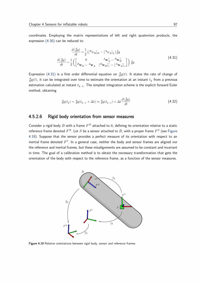
Chapter 4 Sensors for inflatable robots 97

coordinates. Employing the matrix representations of left and right quaternion products, the

expression (4.30) can be reduced to:

𝑑( 𝑞𝐵𝐴 )

𝑑𝑡=1

2([ 𝑤𝐵 𝐵 ]𝑅 − [ 𝑤𝐴

𝐴 ]𝐿) 𝑞𝐵𝐴

𝑑( 𝑞𝐵𝐴 )

𝑑𝑡=1

2([

0 𝐰𝐴⊺

𝐴 − 𝐰𝐵

⊺ 𝐵

𝐰𝐵 𝐵 − 𝐰𝐴

𝐴 [ 𝐰𝐵 𝐵 ]×

⊺ − [ 𝐰𝐴 𝐴 ]×

]) 𝑞𝐵𝐴

(4.31)

Expression (4.31) is a first order differential equation on 𝑞𝐵𝐴 (𝑡). It states the rate of change of

𝑞𝐵𝐴 (𝑡), it can be integrated over time to estimate the orientation at an instant 𝑡𝑘 from a previous

estimation calculated at instant 𝑡𝑘−1. The simplest integration scheme is the explicit forward Euler

method, obtaining

𝑞𝐵𝐴 (𝑡𝑘) = 𝑞𝐵

𝐴 (𝑡𝑘−1 +∆𝑡) ≈ 𝑞𝐵𝐴 (𝑡𝑘−1) + ∆𝑡

𝑑( 𝑞𝐵𝐴 )

𝑑𝑡 (4.32)

4.5.2.6 Rigid body orientation from sensor measures

Consider a rigid body 𝐵 with a frame 𝐹𝐵 attached to it, defining its orientation relative to a static

reference frame denoted 𝐹𝑅. Let 𝑆 be a sensor attached to 𝐵, with a proper frame 𝐹𝑆 (see Figure

4.19). Suppose that the sensor provides a perfect measure of its orientation with respect to an

inertial frame denoted 𝐹 𝐼 . In a general case, neither the body and sensor frames are aligned nor

the reference and inertial frames, but these misalignments are assumed to be constant and invariant

in time. The goal of a calibration method is to obtain the necessary transformation that gets the

orientation of the body with respect to the reference frame, as a function of the sensor measures.

Figure 4.19 Relative orientations between rigid body, sensor and reference frames

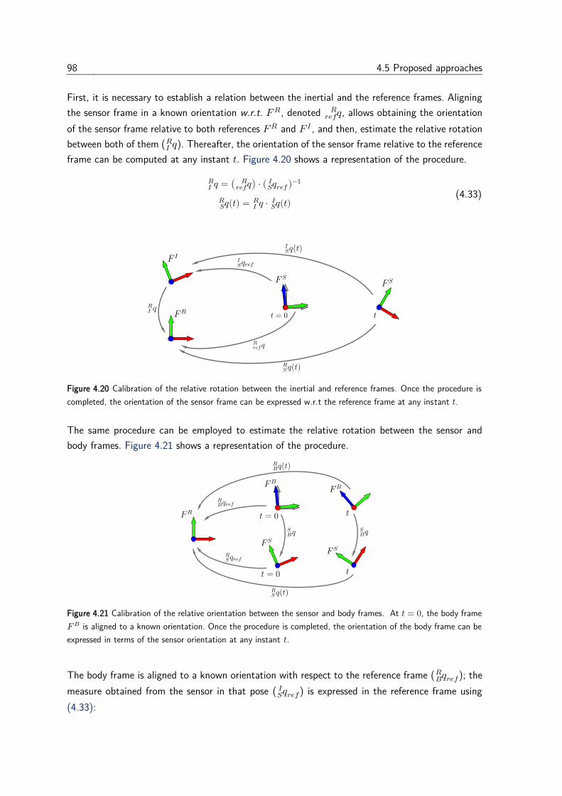
98 4.5 Proposed approaches

First, it is necessary to establish a relation between the inertial and the reference frames. Aligning

the sensor frame in a known orientation w.r.t. 𝐹𝑅, denoted 𝑞𝑟𝑒𝑓𝑅 , allows obtaining the orientation

of the sensor frame relative to both references 𝐹𝑅 and 𝐹 𝐼 , and then, estimate the relative rotation

between both of them ( 𝑞𝐼 𝑅 ). Thereafter, the orientation of the sensor frame relative to the reference

frame can be computed at any instant 𝑡. Figure 4.20 shows a representation of the procedure.

𝑞𝐼 𝑅 = ( 𝑞𝑟𝑒𝑓

𝑅 ) ⋅ ( 𝑞𝑟𝑒𝑓𝑆𝐼 )−1

𝑞𝑆𝑅 (𝑡) = 𝑞𝐼

𝑅 ⋅ 𝑞𝑆𝐼 (𝑡)

(4.33)

Figure 4.20 Calibration of the relative rotation between the inertial and reference frames. Once the procedure is

completed, the orientation of the sensor frame can be expressed w.r.t the reference frame at any instant 𝑡.

The same procedure can be employed to estimate the relative rotation between the sensor and

body frames. Figure 4.21 shows a representation of the procedure.

Figure 4.21 Calibration of the relative orientation between the sensor and body frames. At 𝑡 = 0, the body frame

𝐹𝐵 is aligned to a known orientation. Once the procedure is completed, the orientation of the body frame can be

expressed in terms of the sensor orientation at any instant 𝑡.

The body frame is aligned to a known orientation with respect to the reference frame ( 𝑞𝑟𝑒𝑓𝐵𝑅 ); the

measure obtained from the sensor in that pose ( 𝑞𝑟𝑒𝑓𝑆𝐼 ) is expressed in the reference frame using

(4.33):

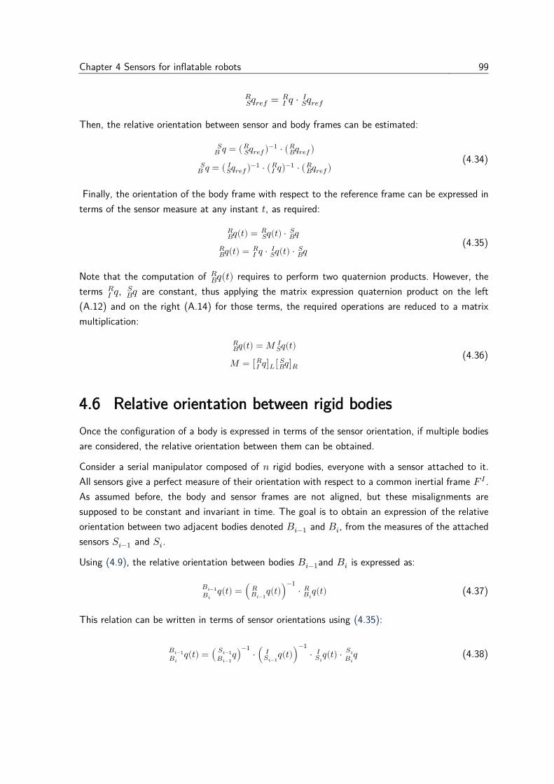
Chapter 4 Sensors for inflatable robots 99

𝑞𝑟𝑒𝑓𝑆𝑅 = 𝑞𝐼

𝑅 ⋅ 𝑞𝑟𝑒𝑓𝑆𝐼

Then, the relative orientation between sensor and body frames can be estimated:

𝑞𝐵 𝑆 = ( 𝑞𝑟𝑒𝑓𝑆

𝑅 )−1 ⋅ ( 𝑞𝑟𝑒𝑓𝐵𝑅 )

𝑞𝐵 𝑆 = ( 𝑞𝑟𝑒𝑓𝑆

𝐼 )−1 ⋅ ( 𝑞𝐼 𝑅 )−1 ⋅ ( 𝑞𝑟𝑒𝑓𝐵

𝑅 ) (4.34)

Finally, the orientation of the body frame with respect to the reference frame can be expressed in

terms of the sensor measure at any instant 𝑡, as required:

𝑞𝐵𝑅 (𝑡) = 𝑞𝑆

𝑅 (𝑡) ⋅ 𝑞𝐵𝑆

𝑞𝐵𝑅 (𝑡) = 𝑞𝐼

𝑅 ⋅ 𝑞𝑆𝐼 (𝑡) ⋅ 𝑞𝐵

𝑆 (4.35)

Note that the computation of 𝑞𝐵𝑅 (𝑡) requires to perform two quaternion products. However, the

terms 𝑞𝐼 𝑅 , 𝑞𝐵

𝑆 are constant, thus applying the matrix expression quaternion product on the left

(A.12) and on the right (A.14) for those terms, the required operations are reduced to a matrix

multiplication:

𝑞𝐵𝑅 (𝑡) = 𝑀 𝑞𝑆

𝐼 (𝑡)

𝑀 = [ 𝑞𝐼 𝑅 ]𝐿[ 𝑞𝐵

𝑆 ]𝑅 (4.36)

4.6 Relative orientation between rigid bodies

Once the configuration of a body is expressed in terms of the sensor orientation, if multiple bodies

are considered, the relative orientation between them can be obtained.

Consider a serial manipulator composed of 𝑛 rigid bodies, everyone with a sensor attached to it.

All sensors give a perfect measure of their orientation with respect to a common inertial frame 𝐹 𝐼 .

As assumed before, the body and sensor frames are not aligned, but these misalignments are

supposed to be constant and invariant in time. The goal is to obtain an expression of the relative

orientation between two adjacent bodies denoted 𝐵𝑖−1 and 𝐵𝑖, from the measures of the attached

sensors 𝑆𝑖−1 and 𝑆𝑖.

Using (4.9), the relative orientation between bodies 𝐵𝑖−1and 𝐵𝑖 is expressed as:

𝑞𝐵𝑖

𝐵𝑖−1 (𝑡) = ( 𝑞𝐵𝑖−1𝑅 (𝑡))

−1

⋅ 𝑞𝐵𝑖𝑅 (𝑡) (4.37)

This relation can be written in terms of sensor orientations using (4.35):

𝑞𝐵𝑖

𝐵𝑖−1 (𝑡) = ( 𝑞𝐵𝑖−1

𝑆𝑖−1 )−1⋅ ( 𝑞𝑆𝑖−1𝐼 (𝑡))

−1

⋅ 𝑞𝑆𝑖𝐼 (𝑡) ⋅ 𝑞

𝐵𝑖

𝑆𝑖 (4.38)

100 4.7 Conclusions

It may be convenient to express the relative orientation at an instant 𝑡 with respect to a reference

configuration of the serial manipulator, in which the orientation of every segment is known. For

instance, in serial manipulators, there is a reference configuration where all joint variables are equal

to zero, and body frames are defined following a convention, for instance, the Denavit-Hartenberg

parameterisation. Thus, when the bodies are aligned in that configuration, the obtained relative

orientations are entity quaternions, and subsequent rotations are measured w.r.t that configuration.

Furthermore, as the body orientations in that configuration are known, they can be used as the

orientation reference ( 𝑞𝑟𝑒𝑓𝐵𝑖𝑅 ) to estimate the sensor to body rotation, described in the last section.

The relative orientation from the reference configuration is defined as follows:

Using (4.38) in (4.39), the complete expression of the relative orientation between two bodies is

obtained in terms of the sensor measures:

This expression can be reduced to a matrix multiplication: group the product of the first three

constant terms in an auxiliary quaternion 𝑢, and denote 𝑣 the constant term at the end. Then use

the matrix representation of left and right quaternion product for 𝑢 and 𝑣 respectively:

𝑞𝑖(𝑡) = 𝑊( 𝑞(𝑡)𝑆𝑖

𝑆𝑖−1 )

𝑊 = [𝑢]𝐿[𝑣]𝑅 (4.41)

Note the simplification of the notation employed in the product of sensor measures: 𝑞(𝑡)𝑆𝑖

𝑆𝑖−1

represents the relative orientation of the sensor 𝑆𝑖 w.r.t the sensor 𝑆𝑖−1. Therefore, it is not

required to know the absolute orientation of every sensor, but rather their relative configuration.

4.7 Conclusions

As conventional manipulators, inflatable robots also need a system of sensors to get feedback of

the actual robot state that will be used in the control loop to converge towards a setpoint. Due to

multiple requirements related to lightness, compliance, and deformability, conventional sensors such

as potentiometers, encoders or resolvers are discarded. Other solutions based on resistive and

capacitive sensing, fiber optics, and exteroceptive sensing are starting to find applications in soft

robotics. In this work, we decided to explore MARG sensors, proposing a network of such sensors

deployed through the entire inflatable structure, intending to estimate the orientation of every link

and thus, the configuration of the whole robot.

𝑞𝑖(𝑡) = ( 𝑞𝑟𝑒𝑓𝐵𝑖

𝐵𝑖−1 )−1

𝑞𝐵𝑖

𝐵𝑖−1 (𝑡)

𝑞𝑟𝑒𝑓𝐵𝑖

𝐵𝑖−1 = ( 𝑞𝑟𝑒𝑓𝐵𝑖−1𝑅 )

−1⋅ ( 𝑞𝑟𝑒𝑓𝐵𝑖𝑅 )

(4.39)

𝑞𝑖(𝑡) = ( 𝑞𝑟𝑒𝑓𝐵𝑖𝑅 )

−1⋅ ( 𝑞𝑟𝑒𝑓𝐵𝑖−1𝑅 ) ⋅ ( 𝑞

𝐵𝑖−1

𝑆𝑖−1 )−1

⏟ 𝑢

⋅ ( 𝑞𝑆𝑖−1𝐼 (𝑡))

−1

⋅ 𝑞𝑆𝑖𝐼 (𝑡)

⏟

𝑞(𝑡)𝑆𝑖

𝑆𝑖−1

⋅ 𝑞𝐵𝑖

𝑆𝑖

⏟𝑣

(4.40)

Chapter 4 Sensors for inflatable robots 101

A first approach was introduced using a 3-axis magnetometer fixed in one of the segments and

perturbed by a permanent magnet attached to the consecutive link. The results performed in a test

bed showed that it is possible to get an accurate estimation of the relative angular position by

observing the variations of the magnetic field. The implementation on the inflatable robot was

more difficult because the supports to which the sensor and magnet were attached were deformed

due to the actuation of the joints, which affected the sensor repeatability of the measures. Future

work could be steered in two directions: The first one could consider the utilization of more sensors,

which would raise more information and improve the robustness of the approach. This consideration

has been used in (Kortier et al., 2015) where the authors proposed an interesting method using a

constellation of magnetometers perturbed by a mobile permanent magnet that had also attached an

inertial sensor. The study aimed to estimate the relative pose of a user’s hand (where the permanent

magnet was attached), and his trunk (which supported the sensor constellation), and showed good

results of the estimation of position and orientation of the hand. The second direction could be focused

on the implementation of alternatives to the mapping between magnetic field readings and angular

position. Here we proposed a simple method based on a gradient descent algorithm, but other

approaches can be explored such as neural networks or machine learning techniques, which can tackle

measures subjected to hysteresis phenomena in a better way. For instance, (Han et al., 2018) proposed

a recurrent neural network for estimating the magnitude and the location of contact pressure in a

microfluidic soft sensor, which also presented hysteretic behavior.

In order to take full advantage of all the available measures in every MARG sensor, a relative orientation

approach was developed. It introduces a new closed solution for orientation estimation from two sets

of vector observations, which can be seen as a generalization of an existing method. The improvement

lies on the independence of the chosen reference vectors, therefore, it is possible to estimate the relative

orientation between two mobile frames directly, instead of determining their absolute orientation w.r.t

a fixed frame and then finding the relative rotation. The approach also considers the relative orientation

estimation from angle rate measurements in both mobile frames. Finally, both estimations are fused in

a complementary filter structure, leading to a more reliable estimation. The approach was validated

through simulation but the experimental implementation is pending which will be part of future work.

Further developments could be focused on the calibration of the sensor to body relative orientation.

Our work focused on orientation estimation but position estimation could also be considered. The main

problem of position estimation using inertial sensors is the drift over time, due to the integration of

noisy signals. However, given that the sensors are attached to the links of a serial chain instead of being

free-floating, there are kinematic constraints that are introduced, which could be exploited jointly with

the geometrical and kinematic model of the robot, to get an estimation robust to dynamical effects.

The principle of this approach can be found in (Kok et al., 2014; Laidig et al., 2017).

Although both proposed methods may appear disjunctive, they are complementary. The use of a

permanent magnet as a more reliable magnetic reference source could be integrated into the estimation

of relative orientation because one of its strengths is that no prior knowledge about the reference field

is required. To get a more uniform magnetic field using permanent magnets, it could be interesting to

experiment with other magnet arrangements, for instance, the Halbach array (Halbach, 1981) that

102 4.7 Conclusions

increases the magnetic field on one side of the array while canceling the field near to zero on the other

side.

Finally, the proliferation of fiber optic sensors applications could lead to a cost reduction and become

an affordable solution for shape sensing systems. It would be an important step in the development of

a robot immune to electromagnetic fields and maybe, ionizing radiation. Moreover, the development of

specific fiber optic that can support repetitive fold and unfold could be valuable research thematics in

terms of materials development and aging and durability studies too.

Chapter 5

Modeling and control of the

inflatable joint

Everything should be as simple as possible,

but no simpler

― Albert Einstein (Attributed by Roger Sessions)

Contents

5.1 Introduction ......................................................................................................... 104

5.2 Setup description ................................................................................................. 106

5.3 Model of the driving circuit ................................................................................... 107

5.3.1 Mechanical subsystem .................................................................................... 107

5.3.2 Pneumatic chambers ...................................................................................... 108

5.3.3 Valve ............................................................................................................ 112

5.3.4 Pipe .............................................................................................................. 114

5.3.5 Complete model ............................................................................................ 115

5.4 Position control.................................................................................................... 117

5.4.1 Related works ................................................................................................ 117

5.4.2 Sliding mode approach ................................................................................... 117

5.4.3 Three-modes controller .................................................................................. 118

5.4.4 Five-modes controller ..................................................................................... 119

5.5 Experimental results ............................................................................................. 120

5.5.1 3 modes Controller ........................................................................................ 120

5.6 Conclusions ......................................................................................................... 121

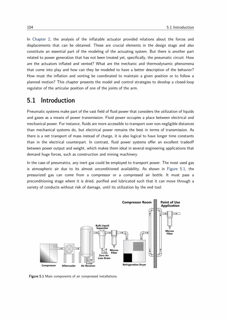
104 5.1 Introduction

In Chapter 2, the analysis of the inflatable actuator provided relations about the forces and

displacements that can be obtained. These are crucial elements in the design stage and also

constitute an essential part of the modeling of the actuating system. But there is another part

related to power generation that has not been treated yet, specifically, the pneumatic circuit. How

are the actuators inflated and vented? What are the mechanic and thermodynamic phenomena

that come into play and how can they be modeled to have a better description of the behavior?

How must the inflation and venting be coordinated to maintain a given position or to follow a

planned motion? This chapter presents the model and control strategies to develop a closed-loop

regulator of the articular position of one of the joints of the arm.

5.1 Introduction

Pneumatic systems make part of the vast field of fluid power that considers the utilization of liquids

and gases as a means of power transmission. Fluid power occupies a place between electrical and

mechanical power. For instance, fluids are more accessible to transport over non-negligible distances

than mechanical systems do, but electrical power remains the best in terms of transmission. As

there is a net transport of mass instead of charge, it is also logical to have longer time constants

than in the electrical counterpart. In contrast, fluid power systems offer an excellent tradeoff

between power output and weight, which makes them ideal in several engineering applications that

demand huge forces, such as construction and mining machinery.

In the case of pneumatics, any inert gas could be employed to transport power. The most used gas

is atmospheric air due to its almost unconditioned availability. As shown in Figure 5.1, the

pressurized gas can come from a compressor or a compressed air bottle. It must pass a

preconditioning stage where it is dried, purified and lubricated such that it can move through a

variety of conducts without risk of damage, until its utilization by the end tool.

Figure 5.1 Main components of air compressed installations.

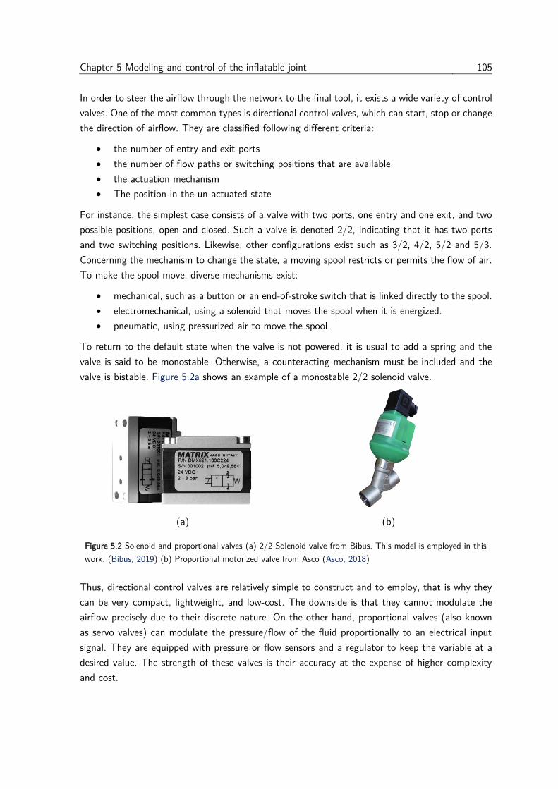
Chapter 5 Modeling and control of the inflatable joint 105

In order to steer the airflow through the network to the final tool, it exists a wide variety of control

valves. One of the most common types is directional control valves, which can start, stop or change

the direction of airflow. They are classified following different criteria:

• the number of entry and exit ports

• the number of flow paths or switching positions that are available

• the actuation mechanism

• The position in the un-actuated state

For instance, the simplest case consists of a valve with two ports, one entry and one exit, and two

possible positions, open and closed. Such a valve is denoted 2/2, indicating that it has two ports

and two switching positions. Likewise, other configurations exist such as 3/2, 4/2, 5/2 and 5/3.

Concerning the mechanism to change the state, a moving spool restricts or permits the flow of air.

To make the spool move, diverse mechanisms exist:

• mechanical, such as a button or an end-of-stroke switch that is linked directly to the spool.

• electromechanical, using a solenoid that moves the spool when it is energized.

• pneumatic, using pressurized air to move the spool.

To return to the default state when the valve is not powered, it is usual to add a spring and the

valve is said to be monostable. Otherwise, a counteracting mechanism must be included and the

valve is bistable. Figure 5.2a shows an example of a monostable 2/2 solenoid valve.

(a) (b)

Figure 5.2 Solenoid and proportional valves (a) 2/2 Solenoid valve from Bibus. This model is employed in this

work. (Bibus, 2019) (b) Proportional motorized valve from Asco (Asco, 2018)

Thus, directional control valves are relatively simple to construct and to employ, that is why they

can be very compact, lightweight, and low-cost. The downside is that they cannot modulate the

airflow precisely due to their discrete nature. On the other hand, proportional valves (also known

as servo valves) can modulate the pressure/flow of the fluid proportionally to an electrical input

signal. They are equipped with pressure or flow sensors and a regulator to keep the variable at a

desired value. The strength of these valves is their accuracy at the expense of higher complexity

and cost.

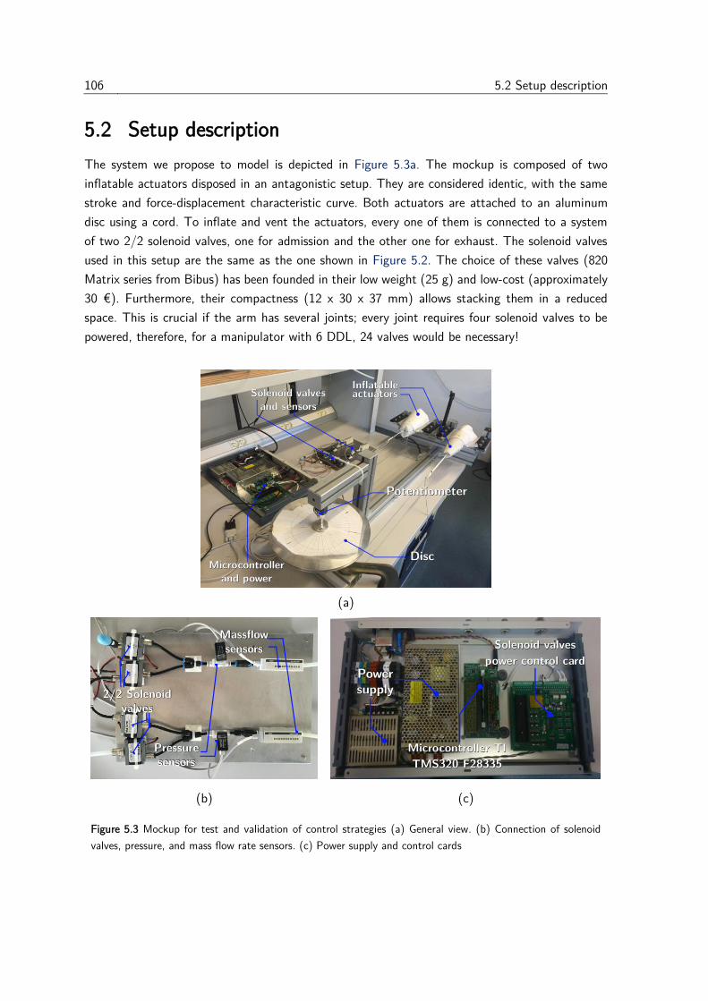
106 5.2 Setup description

5.2 Setup description

The system we propose to model is depicted in Figure 5.3a. The mockup is composed of two

inflatable actuators disposed in an antagonistic setup. They are considered identic, with the same

stroke and force-displacement characteristic curve. Both actuators are attached to an aluminum

disc using a cord. To inflate and vent the actuators, every one of them is connected to a system

of two 2/2 solenoid valves, one for admission and the other one for exhaust. The solenoid valves

used in this setup are the same as the one shown in Figure 5.2. The choice of these valves (820

Matrix series from Bibus) has been founded in their low weight (25 g) and low-cost (approximately

30 €). Furthermore, their compactness (12 x 30 x 37 mm) allows stacking them in a reduced

space. This is crucial if the arm has several joints; every joint requires four solenoid valves to be

powered, therefore, for a manipulator with 6 DDL, 24 valves would be necessary!

(a)

(b) (c)

Figure 5.3 Mockup for test and validation of control strategies (a) General view. (b) Connection of solenoid

valves, pressure, and mass flow rate sensors. (c) Power supply and control cards

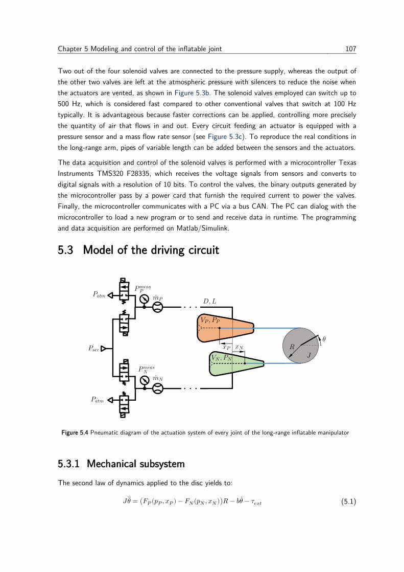
Chapter 5 Modeling and control of the inflatable joint 107

Two out of the four solenoid valves are connected to the pressure supply, whereas the output of

the other two valves are left at the atmospheric pressure with silencers to reduce the noise when

the actuators are vented, as shown in Figure 5.3b. The solenoid valves employed can switch up to

500 Hz, which is considered fast compared to other conventional valves that switch at 100 Hz

typically. It is advantageous because faster corrections can be applied, controlling more precisely

the quantity of air that flows in and out. Every circuit feeding an actuator is equipped with a

pressure sensor and a mass flow rate sensor (see Figure 5.3c). To reproduce the real conditions in

the long-range arm, pipes of variable length can be added between the sensors and the actuators.

The data acquisition and control of the solenoid valves is performed with a microcontroller Texas

Instruments TMS320 F28335, which receives the voltage signals from sensors and converts to

digital signals with a resolution of 10 bits. To control the valves, the binary outputs generated by

the microcontroller pass by a power card that furnish the required current to power the valves.

Finally, the microcontroller communicates with a PC via a bus CAN. The PC can dialog with the

microcontroller to load a new program or to send and receive data in runtime. The programming

and data acquisition are performed on Matlab/Simulink.

5.3 Model of the driving circuit

Figure 5.4 Pneumatic diagram of the actuation system of every joint of the long-range inflatable manipulator

5.3.1 Mechanical subsystem

The second law of dynamics applied to the disc yields to:

𝐽𝜃 ̈ = (𝐹𝑃 (𝑝𝑃 , 𝑥𝑃 ) − 𝐹𝑁 (𝑝𝑁 , 𝑥𝑁 ))𝑅 − 𝑏𝜃̇− 𝜏𝑒𝑥𝑡 (5.1)

108 5.3 Model of the driving circuit

where 𝐽 and 𝑅 are the inertia and radius of the pulley, 𝐹 is the force exerted by every actuator

as a function of the inner pressure 𝑝 and its position 𝑥, 𝑏 is the viscous friction coefficient 𝜏𝑒𝑥𝑡 is

the sum of all external torques. Subindices 𝑃 and 𝑁 denote positive and negative to clarify the

direction in which every actuator drives the joint. As it was shown in Chapter 3, the force developed

by every actuator depends on the pressure and the position. The model developed in Chapter 3 is

employed here. It is worth to note that the zero position is in the middle of the stroke. Noting the

total stroke of every actuator as 𝐿, the position employed in this model and that one used in

Chapter 3 are related through:

𝑥𝑃 = 𝑥 −𝐿

2 (5.2)

The relation between the angular displacement and the linear displacements of each actuator is

described through the arc length:

𝑥𝑃 = 𝑅𝜃 𝑥𝑁 = −𝑅𝜃 (5.3)

5.3.2 Pneumatic chambers

The evolution of the volume, pressure, and temperature in every actuator are intrinsically linked

and their evolution can be studied and modelled through a thermodynamic analysis. It will be

assumed that:

• The air behaves as a perfect gas

• The kinetic energy inside the chamber is negligible respect to the kinetic energy of the

fluid at input and output ports

• The work exchange is reversible

• The distribution of mass, pressure, and temperature inside the chamber is uniform

The actuator can be considered as an open system; the envelope delimits a control volume that

exchanges heat and mechanical work with the environment, for instance, by displacing an object,

changing its shape, or suffering a displacement caused by an external force. On the other hand,

the exchange of mass must be also considered, it can come from inlet and outlet mass flow or

possible leakages. The principle of energy conservation in an open system takes into account not

only the exchange of energy in the form of heat and work but also the energy that gets in and out

due to the mass exchange (Wark and Richards, 1999):

𝑑𝐸𝑐𝑣𝑑𝑡= �̇�𝑐𝑣 + �̇�𝑐𝑣 + �̇�𝑖 (ℎ𝑖 +

𝑣𝑖2

2+ 𝑔𝑧𝑖) − �̇�𝑜 (ℎ𝑜 +

𝑣𝑜2

2+ 𝑔𝑧𝑜) (5.4)

𝐸𝑐𝑣 is the total energy of the control volume, �̇�𝑐𝑣 is the net rate of heat transfer into the control

volume, �̇�𝑐𝑣 is the rate of work done into the control volume, �̇� is the mass flow rate, ℎ is the

specific enthalpy, 𝑣 is the speed of the gas, 𝑔 is the gravitational acceleration and 𝑧 the heigh

respect to an arbitrary reference. Subindices 𝑖 and 𝑜 stand for input and output, and 𝑐𝑣 for the

Chapter 5 Modeling and control of the inflatable joint 109

control volume. Considering a homogeneous distribution of gas in the control volume, the total

energy comprising the internal, kinetic and potential energy, can be written as:

𝐸𝑐𝑣 = 𝑚𝑐𝑣 (𝑢𝑐𝑣 +1

2𝑣 ̅2 + 𝑔𝑧)̅ (5.5)

However, the speed of the gas inside the chamber (𝑣)̅ is negligible compared to the speed close to

the input and output ports, and its contribution to the total energy can be discarded. Furthermore,

the change of potential energy is minimal in this case; thus, the associated terms in expressions

(5.4) and (5.5) can be neglected. With these assumptions, the expression (5.4) reduces to:

𝑑(𝑚𝑐𝑣𝑢𝑐𝑣)

𝑑𝑡= �̇�𝑐𝑣 + �̇�𝑐𝑣 + �̇�𝑖 (ℎ𝑖 +

𝑣𝑖2

2) − �̇�𝑜 (ℎ𝑜 +

𝑣𝑜2

2) (5.6)

In a thermodynamic system, the enthalpy is defined as the sum of the internal energy (𝑈) and

the amount of work required to take the system to its volume and pressure conditions :

𝐻 = 𝑈 + 𝑝𝑉 (5.7)

Likewise, the specific enthalpy (ℎ) describes the total enthalpy per unit of mass in a thermodynamic

system:

ℎ = 𝑢 + 𝑝𝑉

𝑚 (5.8)

Where 𝑢 is the specific internal energy. In order to get an expression for 𝑢, let us recall the concept

of specific heat capacity of a substance. It is defined as an intrinsic property that relates the amount

of heat required to induce a unit change of temperature in a unit mass of the substance. The heat

capacity depends on the thermodynamic process. Imagine a cylinder that is heated and consider

two situations:

• The piston can slide such that the pressure remains constant (this is called an isobaric

process) while the gas inside is heated. The heat added to the system contributes not

only to increase the gas temperature but also generates work due to the gas expansion.

In this case, the specific heat capacity is denoted 𝑐𝑝.

• The piston is fixed such that the volume remains constant (this is called an isochoric

process). Given that there is no possible expansion, the produced work is zero and the

heat supplied contributes entirely to the change of the internal energy. In this case, the

specific heat capacity at constant volume is denoted 𝑐𝑣.

When considering a perfect gas, the internal energy is a function of a unique independent variable,

the temperature. Therefore, the specific internal energy is given by the product of its specific heat

capacity at constant volume and its change of temperature:

𝑢 = 𝑐𝑣(𝑇 − 𝑇0) (5.9)

110 5.3 Model of the driving circuit

Both heat capacities are related through the heat capacity ratio (𝛾):

𝛾 =𝑐𝑝𝑐𝑣

(5.10)

For instance, ideal monoatomic gases have a heat capacity ratio of 1.667, while for diatomic gases

it is 1.4, very close to the ratio of dry air.

Under the assumption of perfect gas; the general gas equation states a relation between pressure,

volume, mass and temperature:

𝑝𝑉 = 𝑚𝑟𝑇 (5.11)

Where 𝑝 is the pressure of the gas, 𝑉 the volume, 𝑚 the total mass of gas, 𝑇 the absolute

temperature and 𝑟 the universal gas constant specific to the considered gas. It is determined by

the ratio of the ideal gas constant 𝑅 (8.314 J/(K·mol)) and the molar mass of the considered gas.

For instance, the molar mass for dry air is 28.96 g/mol; thus, the specific gas constant is 287.0

J/(K·kg).

Furthermore, in the case of a perfect gas, both specific heat capacities 𝑐𝑣 and 𝑐𝑝 are related through

the Mayers relation:

𝑐𝑝 − 𝑐𝑣 = 𝑟 (5.12)

Other expressions can be obtained using (5.12) in (5.8), (5.9) and (5.10):

𝑐𝑣 =𝑟

𝛾 − 1 𝑐𝑝 =

𝛾𝑟

𝛾 − 1 (5.13)

ℎ = 𝑐𝑝𝑇 − 𝑐𝑣𝑇0 (5.14)

With these relations, the total energy in the control volume is rewritten and differentiated w.r.t

time:

𝑑(𝑚𝑐𝑣𝑢𝑐𝑣)

𝑑𝑡=𝑑

𝑑𝑡(𝑚𝑐𝑣𝑐𝑣(𝑇𝑐𝑣 − 𝑇0)) =

𝑑

𝑑𝑡(𝑐𝑣𝑟𝑝𝑐𝑣𝑉𝑐𝑣) − �̇�𝑐𝑣𝑐𝑣𝑇0 (5.15)

Where 𝑝𝑐𝑣, 𝑉𝑐𝑣 and �̇�𝑐𝑣 correspond to the pressure, the volume and the mass flow rate in the

control volume. This last term is equal to the difference between the input and the output mass

flow rates, namely �̇�𝑖 − �̇�𝑜. Introducing (5.14) and (5.15) into (5.6), it yields to:

𝑑

𝑑𝑡(𝑐𝑣𝑟𝑝𝑐𝑣𝑉𝑐𝑣) = �̇�𝑐𝑣 + �̇�𝑐𝑣 + �̇�𝑖 (𝑐𝑝𝑇𝑖 +

𝑣𝑖2

2) − �̇�𝑜 (𝑐𝑝𝑇𝑜 +

𝑣𝑜2

2) (5.16)

Where 𝑇𝑖 and 𝑇𝑜 are the temperatures of the air at the inlet and the outlet, respectively. By

considering a uniform distribution of temperature, it can be assumed that the temperature at the

outlet is equal to the temperature inside the chamber, namely 𝑇𝑜 = 𝑇𝑐𝑣. Assuming that the work

Chapter 5 Modeling and control of the inflatable joint 111

done into the control volume is reversible, its rate of change can be linked directly to the volume

change:

�̇�𝑐𝑣 = −𝑝𝑉�̇�𝑣 (5.17)

In a pneumatic system, most of the energy is furnished from the fluid pressure, more than the

kinetic energy that can have the fluid. Therefore, in this particular case, the terms related to the

kinetic energy in the expression (5.16) can be neglected, and it is reduced to:

𝑝�̇�𝑣𝑉𝑐𝑣 = (𝛾 − 1)�̇�𝑐𝑣 − 𝛾𝑝𝑐𝑣𝑉�̇�𝑣 + 𝛾𝑟(�̇�𝑖𝑇𝑖) − 𝛾𝑟(�̇�𝑜𝑇𝑐𝑣) (5.18)

𝑝�̇�𝑣 =𝛾

𝑉𝑐𝑣((𝛾 − 1)

𝛾�̇�𝑐𝑣 − 𝑝𝑐𝑣𝑉�̇�𝑣 + 𝑟�̇�𝑖𝑇𝑖 − 𝑟�̇�𝑜𝑇𝑐𝑣) (5.19)

Multiples cases can be considered depending on the type of thermodynamic process:

• In an adiabatic process, there is no heat exchange, therefore (5.19) reduces to:

𝑝�̇�𝑣 =𝛾

𝑉𝑐𝑣(−𝑝𝑐𝑣𝑉�̇�𝑣 + 𝑟�̇�𝑖𝑇𝑖 − 𝑟�̇�𝑜𝑇𝑐𝑣) (5.20)

• In an isentropic process, not only there is no heat exchange, but the temperature is the

same at the inlet and inside the chamber, namely 𝑇𝑖 = 𝑇𝑐𝑣:

𝑝̇𝑐𝑣 =𝛾

𝑉𝑐𝑣(−𝑝𝑐𝑣𝑉�̇�𝑣 + 𝑟𝑇𝑐𝑣�̇�) (5.21)

• In an isothermal process, the temperature remains constant and 𝑇𝑖 = 𝑇𝑐𝑣. By

differentiating the general gas equation (5.11) w.r.t time, and considering that the time

derivative of the temperature is null, it follows:

𝑝̇𝑉 + 𝑝𝑉 ̇ = �̇�𝑟𝑇 (5.22)

Rearranging the terms:

𝑝̇𝑐𝑣 =1

𝑉𝑐𝑣(−𝑝𝑐𝑣𝑉�̇�𝑣 + 𝑟𝑇𝑐𝑣�̇�) (5.23)

In the rest of the analysis, it will be considered that the chambers follow an isentropic process,

therefore, only the expression (5.20) will be employed.

In Chapter 3, the expression relating the volume and the linear displacement was obtained. Once

again, in order to use this expression, the change of reference has to be considered employing (5.2).

Finally, the pressure dynamics in every actuator is described by:

𝑝�̇� ,𝑁 =𝛾

𝑉𝑃,𝑁(𝑥𝑃,𝑁)(−𝑝𝑃,𝑁𝑉�̇� ,𝑁(𝑥𝑃,𝑁) + 𝑟𝑇𝑃,𝑁�̇�𝑃,𝑁) (5.24)

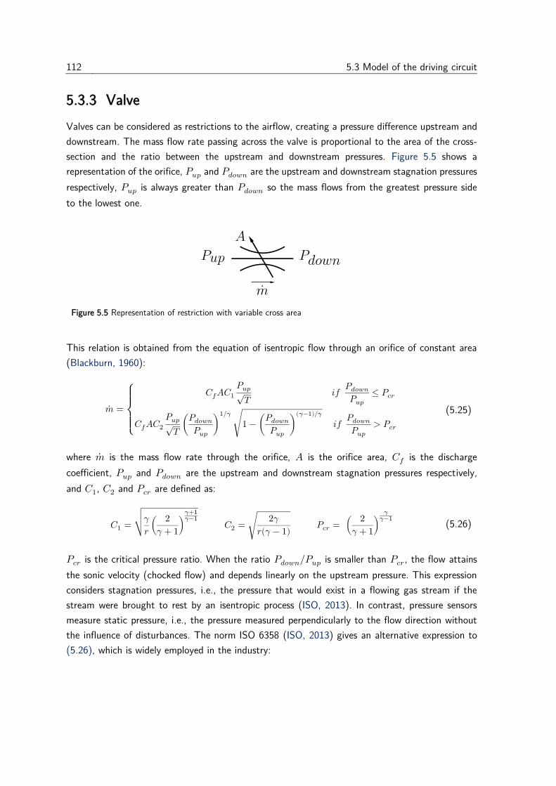
112 5.3 Model of the driving circuit

5.3.3 Valve

Valves can be considered as restrictions to the airflow, creating a pressure difference upstream and

downstream. The mass flow rate passing across the valve is proportional to the area of the cross-

section and the ratio between the upstream and downstream pressures. Figure 5.5 shows a

representation of the orifice, 𝑃𝑢𝑝 and 𝑃𝑑𝑜𝑤𝑛 are the upstream and downstream stagnation pressures

respectively, 𝑃𝑢𝑝 is always greater than 𝑃𝑑𝑜𝑤𝑛 so the mass flows from the greatest pressure side

to the lowest one.

Figure 5.5 Representation of restriction with variable cross area

This relation is obtained from the equation of isentropic flow through an orifice of constant area

(Blackburn, 1960):

�̇� =

{

𝐶𝑓𝐴𝐶1𝑃𝑢𝑝√𝑇

𝑖𝑓 𝑃𝑑𝑜𝑤𝑛𝑃𝑢𝑝

≤ 𝑃𝑐𝑟

𝐶𝑓𝐴𝐶2𝑃𝑢𝑝√𝑇(𝑃𝑑𝑜𝑤𝑛𝑃𝑢𝑝)1/𝛾

√1−(𝑃𝑑𝑜𝑤𝑛𝑃𝑢𝑝)(𝛾−1)/𝛾

𝑖𝑓 𝑃𝑑𝑜𝑤𝑛𝑃𝑢𝑝

> 𝑃𝑐𝑟

(5.25)

where �̇� is the mass flow rate through the orifice, 𝐴 is the orifice area, 𝐶𝑓 is the discharge

coefficient, 𝑃𝑢𝑝 and 𝑃𝑑𝑜𝑤𝑛 are the upstream and downstream stagnation pressures respectively,

and 𝐶1, 𝐶2 and 𝑃𝑐𝑟 are defined as:

𝐶1 =√

𝛾

𝑟(2

𝛾 + 1)

𝛾+1𝛾−1 𝐶2 = √

2𝛾

𝑟(𝛾 − 1) 𝑃𝑐𝑟 = (

2

𝛾 + 1)

𝛾𝛾−1

(5.26)

𝑃𝑐𝑟 is the critical pressure ratio. When the ratio 𝑃𝑑𝑜𝑤𝑛 𝑃𝑢𝑝⁄ is smaller than 𝑃𝑐𝑟, the flow attains

the sonic velocity (chocked flow) and depends linearly on the upstream pressure. This expression

considers stagnation pressures, i.e., the pressure that would exist in a flowing gas stream if the

stream were brought to rest by an isentropic process (ISO, 2013). In contrast, pressure sensors

measure static pressure, i.e., the pressure measured perpendicularly to the flow direction without

the influence of disturbances. The norm ISO 6358 (ISO, 2013) gives an alternative expression to

(5.26), which is widely employed in the industry:

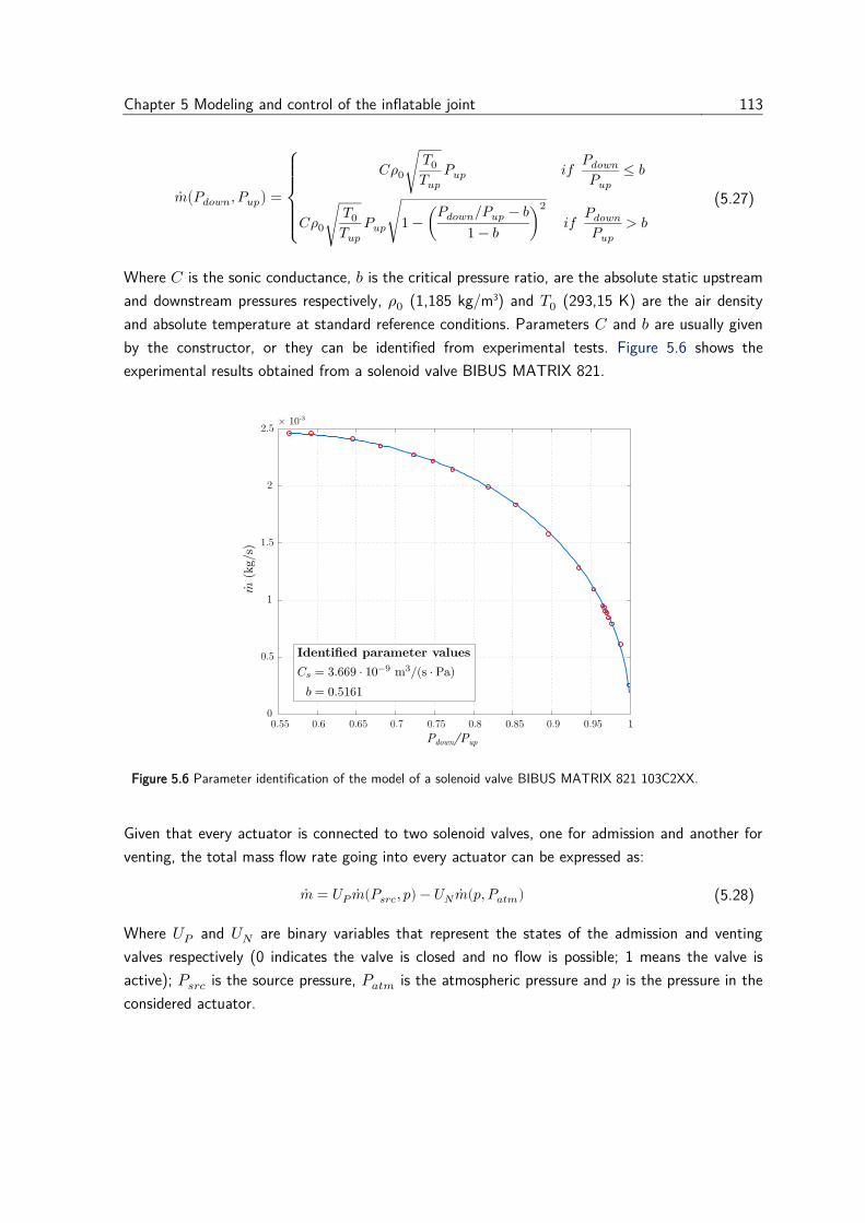
Chapter 5 Modeling and control of the inflatable joint 113

�̇�(𝑃𝑑𝑜𝑤𝑛, 𝑃𝑢𝑝) =

{

𝐶𝜌0√𝑇0𝑇𝑢𝑝𝑃𝑢𝑝 𝑖𝑓

𝑃𝑑𝑜𝑤𝑛𝑃𝑢𝑝

≤ 𝑏

𝐶𝜌0√𝑇0𝑇𝑢𝑝𝑃𝑢𝑝√1 −(

𝑃𝑑𝑜𝑤𝑛 𝑃𝑢𝑝⁄ − 𝑏

1 − 𝑏)

2

𝑖𝑓 𝑃𝑑𝑜𝑤𝑛𝑃𝑢𝑝

> 𝑏

(5.27)

Where 𝐶 is the sonic conductance, 𝑏 is the critical pressure ratio, are the absolute static upstream

and downstream pressures respectively, 𝜌0 (1,185 kg/m3) and 𝑇0 (293,15 K) are the air density

and absolute temperature at standard reference conditions. Parameters 𝐶 and 𝑏 are usually given

by the constructor, or they can be identified from experimental tests. Figure 5.6 shows the

experimental results obtained from a solenoid valve BIBUS MATRIX 821.

Figure 5.6 Parameter identification of the model of a solenoid valve BIBUS MATRIX 821 103C2XX.

Given that every actuator is connected to two solenoid valves, one for admission and another for

venting, the total mass flow rate going into every actuator can be expressed as:

�̇� = 𝑈𝑃 �̇�(𝑃𝑠𝑟𝑐, 𝑝) − 𝑈𝑁�̇�(𝑝, 𝑃𝑎𝑡𝑚) (5.28)

Where 𝑈𝑃 and 𝑈𝑁 are binary variables that represent the states of the admission and venting

valves respectively (0 indicates the valve is closed and no flow is possible; 1 means the valve is

active); 𝑃𝑠𝑟𝑐 is the source pressure, 𝑃𝑎𝑡𝑚 is the atmospheric pressure and 𝑝 is the pressure in the

considered actuator.

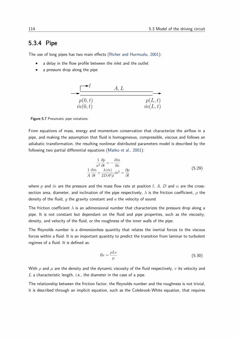
114 5.3 Model of the driving circuit

5.3.4 Pipe

The use of long pipes has two main effects (Richer and Hurmuzlu, 2001):

• a delay in the flow profile between the inlet and the outlet

• a pressure drop along the pipe

Figure 5.7 Pneumatic pipe notations.

From equations of mass, energy and momentum conservation that characterize the airflow in a

pipe, and making the assumption that fluid is homogeneous, compressible, viscous and follows an

adiabatic transformation, the resulting nonlinear distributed parameters model is described by the

following two partial differential equations (Matko et al., 2001):

1

𝑎2𝜕𝑝

𝜕𝑡= −𝜕�̇�

𝜕𝑥1

𝐴

𝜕�̇�

𝜕𝑡+𝜆(�̇�)

2𝐷𝐴2𝜌 ̅�̇�2 =

𝜕𝑝

𝜕𝑙

(5.29)

where 𝑝 and �̇� are the pressure and the mass flow rate at position 𝑙; 𝐴, 𝐷 and 𝛼 are the cross-

section area, diameter, and inclination of the pipe respectively, 𝜆 is the friction coefficient, 𝜌 the

density of the fluid, 𝑔 the gravity constant and 𝑎 the velocity of sound.

The friction coefficient 𝜆 is an adimensional number that characterizes the pressure drop along a

pipe. It is not constant but dependant on the fluid and pipe properties, such as the viscosity,

density, and velocity of the fluid, or the roughness of the inner walls of the pipe.

The Reynolds number is a dimensionless quantity that relates the inertial forces to the viscous

forces within a fluid. It is an important quantity to predict the transition from laminar to turbulent

regimes of a fluid. It is defined as:

𝑅𝑒 =𝜌𝐿𝑣

𝜇 (5.30)

With 𝜌 and 𝜇 are the density and the dynamic viscosity of the fluid respectively, 𝑣 its velocity and

𝐿 a characteristic length, i.e., the diameter in the case of a pipe.

The relationship between the friction factor, the Reynolds number and the roughness is not trivial,

it is described through an implicit equation, such as the Colebrook-White equation, that requires

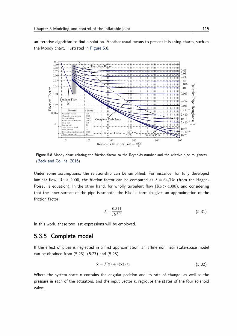
Chapter 5 Modeling and control of the inflatable joint 115

an iterative algorithm to find a solution. Another usual means to present it is using charts, such as

the Moody chart, illustrated in Figure 5.8.

Figure 5.8 Moody chart relating the friction factor to the Reynolds number and the relative pipe roughness

(Beck and Collins, 2016)

Under some assumptions, the relationship can be simplified. For instance, for fully developed

laminar flow, Re < 2000, the friction factor can be computed as 𝜆 = 64 Re⁄ (from the Hagen-

Poiseuille equation). In the other hand, for wholly turbulent flow (Re > 4000), and considering

that the inner surface of the pipe is smooth, the Blasius formula gives an approximation of the

friction factor:

𝜆 =0.314

𝑅𝑒1 4⁄ (5.31)

In this work, these two last expressions will be employed.

5.3.5 Complete model

If the effect of pipes is neglected in a first approximation, an affine nonlinear state-space model

can be obtained from (5.23), (5.27) and (5.28):

�̇� = 𝑓(𝐱) + 𝑔(𝐱) ⋅ 𝐮 (5.32)

Where the system state 𝐱 contains the angular position and its rate of change, as well as the

pressure in each of the actuators, and the input vector 𝐮 regroups the states of the four solenoid

valves:

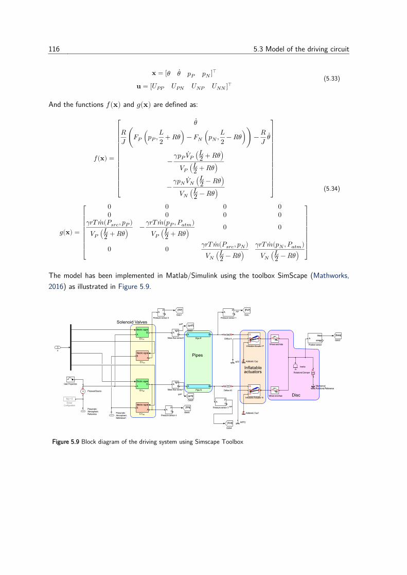
116 5.3 Model of the driving circuit

𝐱 = [𝜃 𝜃 ̇ 𝑝𝑃 𝑝𝑁 ]⊺

𝐮 = [𝑈𝑃𝑃 𝑈𝑃𝑁 𝑈𝑁𝑃 𝑈𝑁𝑁 ]⊺

(5.33)

And the functions 𝑓(𝐱) and 𝑔(𝐱) are defined as:

𝑓(𝐱) =

[

𝜃 ̇

𝑅

𝐽(𝐹𝑃 (𝑝𝑃 ,

𝐿

2+ 𝑅𝜃) − 𝐹𝑁 (𝑝𝑁 ,

𝐿

2− 𝑅𝜃))−

𝑅

𝐽𝜃 ̇

−𝛾𝑝𝑃𝑉�̇� (

𝐿2 + 𝑅𝜃)

𝑉𝑃 (𝐿2 + 𝑅𝜃)

−𝛾𝑝𝑁𝑉�̇� (

𝐿2 − 𝑅𝜃)

𝑉𝑁 (𝐿2 − 𝑅𝜃) ]

𝑔(𝐱) =

[

0 0 0 00 0 0 0

𝛾𝑟𝑇 �̇�(𝑃𝑠𝑟𝑐, 𝑝𝑃 )

𝑉𝑃 (𝐿2 + 𝑅𝜃)

−𝛾𝑟𝑇 �̇�(𝑝𝑃 , 𝑃𝑎𝑡𝑚)

𝑉𝑃 (𝐿2 + 𝑅𝜃)

0 0

0 0𝛾𝑟𝑇 �̇�(𝑃𝑠𝑟𝑐, 𝑝𝑁)

𝑉𝑁 (𝐿2 − 𝑅𝜃)

𝛾𝑟𝑇 �̇�(𝑝𝑁 , 𝑃𝑎𝑡𝑚)

𝑉𝑁 (𝐿2 − 𝑅𝜃) ]

(5.34)

The model has been implemented in Matlab/Simulink using the toolbox SimScape (Mathworks,

2016) as illustrated in Figure 5.9.

Figure 5.9 Block diagram of the driving system using Simscape Toolbox

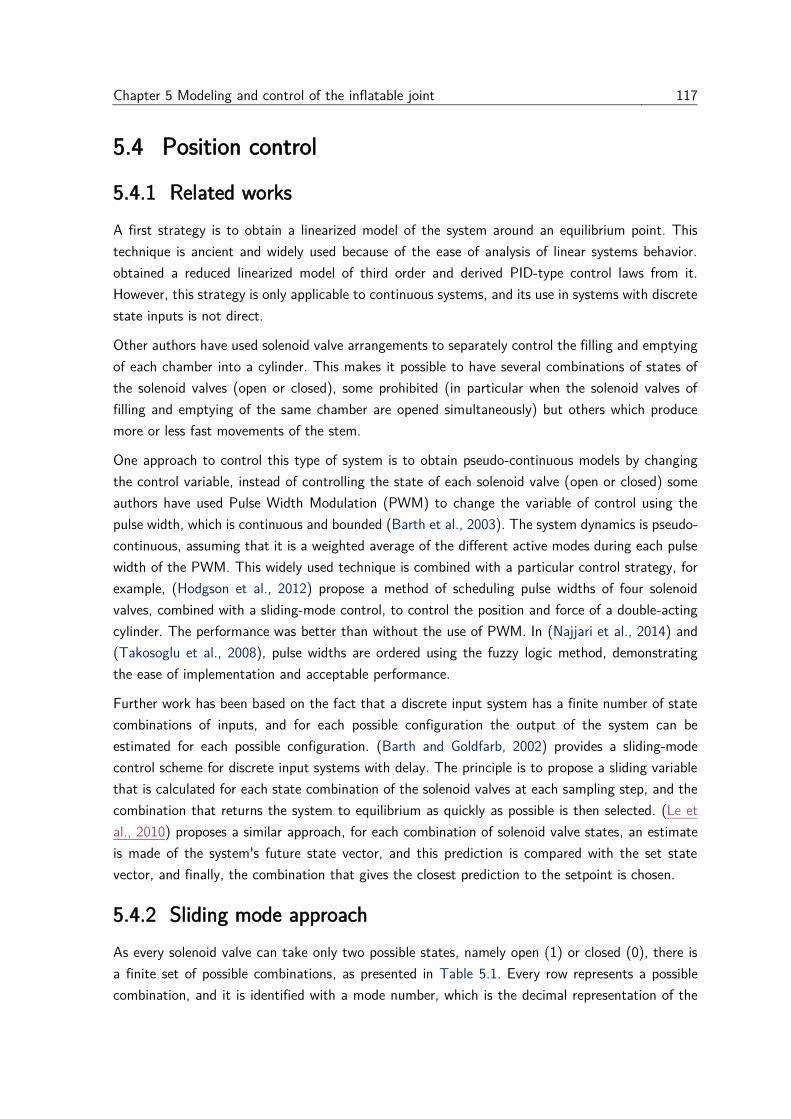
Chapter 5 Modeling and control of the inflatable joint 117

5.4 Position control

5.4.1 Related works

A first strategy is to obtain a linearized model of the system around an equilibrium point. This

technique is ancient and widely used because of the ease of analysis of linear systems behavior.

obtained a reduced linearized model of third order and derived PID-type control laws from it.

However, this strategy is only applicable to continuous systems, and its use in systems with discrete

state inputs is not direct.

Other authors have used solenoid valve arrangements to separately control the filling and emptying

of each chamber into a cylinder. This makes it possible to have several combinations of states of

the solenoid valves (open or closed), some prohibited (in particular when the solenoid valves of

filling and emptying of the same chamber are opened simultaneously) but others which produce

more or less fast movements of the stem.

One approach to control this type of system is to obtain pseudo-continuous models by changing

the control variable, instead of controlling the state of each solenoid valve (open or closed) some

authors have used Pulse Width Modulation (PWM) to change the variable of control using the

pulse width, which is continuous and bounded (Barth et al., 2003). The system dynamics is pseudo-

continuous, assuming that it is a weighted average of the different active modes during each pulse

width of the PWM. This widely used technique is combined with a particular control strategy, for

example, (Hodgson et al., 2012) propose a method of scheduling pulse widths of four solenoid

valves, combined with a sliding-mode control, to control the position and force of a double-acting

cylinder. The performance was better than without the use of PWM. In (Najjari et al., 2014) and

(Takosoglu et al., 2008), pulse widths are ordered using the fuzzy logic method, demonstrating

the ease of implementation and acceptable performance.

Further work has been based on the fact that a discrete input system has a finite number of state

combinations of inputs, and for each possible configuration the output of the system can be

estimated for each possible configuration. (Barth and Goldfarb, 2002) provides a sliding-mode

control scheme for discrete input systems with delay. The principle is to propose a sliding variable

that is calculated for each state combination of the solenoid valves at each sampling step, and the

combination that returns the system to equilibrium as quickly as possible is then selected. (Le et

al., 2010) proposes a similar approach, for each combination of solenoid valve states, an estimate

is made of the system's future state vector, and this prediction is compared with the set state

vector, and finally, the combination that gives the closest prediction to the setpoint is chosen.

5.4.2 Sliding mode approach

As every solenoid valve can take only two possible states, namely open (1) or closed (0), there is

a finite set of possible combinations, as presented in Table 5.1. Every row represents a possible

combination, and it is identified with a mode number, which is the decimal representation of the

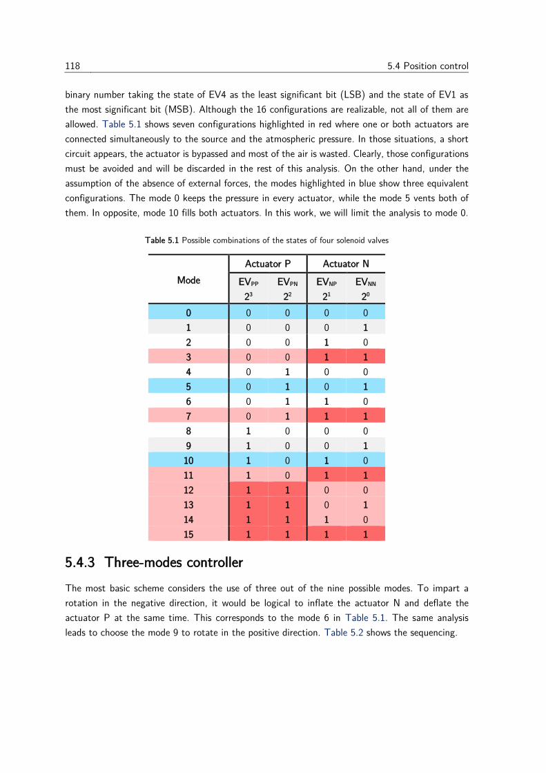
118 5.4 Position control

binary number taking the state of EV4 as the least significant bit (LSB) and the state of EV1 as

the most significant bit (MSB). Although the 16 configurations are realizable, not all of them are

allowed. Table 5.1 shows seven configurations highlighted in red where one or both actuators are

connected simultaneously to the source and the atmospheric pressure. In those situations, a short

circuit appears, the actuator is bypassed and most of the air is wasted. Clearly, those configurations

must be avoided and will be discarded in the rest of this analysis. On the other hand, under the

assumption of the absence of external forces, the modes highlighted in blue show three equivalent

configurations. The mode 0 keeps the pressure in every actuator, while the mode 5 vents both of

them. In opposite, mode 10 fills both actuators. In this work, we will limit the analysis to mode 0.

Table 5.1 Possible combinations of the states of four solenoid valves

Mode

Actuator P Actuator N

EVPP

23

EVPN

22

EVNP

21

EVNN

20

0 0 0 0 0

1 0 0 0 1

2 0 0 1 0

3 0 0 1 1

4 0 1 0 0

5 0 1 0 1

6 0 1 1 0

7 0 1 1 1

8 1 0 0 0

9 1 0 0 1

10 1 0 1 0

11 1 0 1 1

12 1 1 0 0

13 1 1 0 1

14 1 1 1 0

15 1 1 1 1

5.4.3 Three-modes controller

The most basic scheme considers the use of three out of the nine possible modes. To impart a

rotation in the negative direction, it would be logical to inflate the actuator N and deflate the

actuator P at the same time. This corresponds to the mode 6 in Table 5.1. The same analysis

leads to choose the mode 9 to rotate in the positive direction. Table 5.2 shows the sequencing.

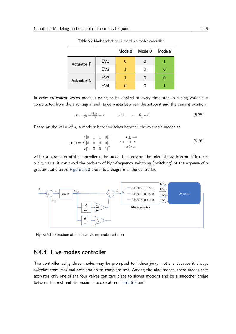
Chapter 5 Modeling and control of the inflatable joint 119

Table 5.2 Modes selection in the three modes controller

Mode 6 Mode 0 Mode 9

Actuator P EV1 0 0 1

EV2 1 0 0

Actuator N EV3 1 0 0

EV4 0 0 1

In order to choose which mode is going to be applied at every time step, a sliding variable is

constructed from the error signal and its derivates between the setpoint and the current position.

𝑠 = 𝑒̈𝜔2+ 2𝜉𝑒̇𝜔+ 𝑒 with 𝑒 = 𝜃𝑐 − 𝜃 (5.35)

Based on the value of 𝑠, a mode selector switches between the available modes as:

𝐮(𝑠) =

{

[0 1 1 0]⊺

[0 0 0 0]⊺

[1 0 0 1]⊺

𝑠 ≤ −𝜖−𝜖 < 𝑠 < 𝜖 𝑠 ≥ 𝜖

(5.36)

with 𝜖 a parameter of the controller to be tuned. It represents the tolerable static error. If it takes

a big, value, it can avoid the problem of high-frequency switching (switching) at the expense of a

greater static error. Figure 5.10 presents a diagram of the controller.

Figure 5.10 Structure of the three sliding mode controller

5.4.4 Five-modes controller

The controller using three modes may be prompted to induce jerky motions because it always

switches from maximal acceleration to complete rest. Among the nine modes, there modes that

activates only one of the four valves can give place to slower motions and be a smoother bridge

between the rest and the maximal acceleration. Table 5.3 and

𝑑

𝑑𝑡

System𝑒 𝑠

+++-

Mode 0 [0 0 0 0]

Mode 6 [0 1 1 0]

Mode 9 [1 0 0 1]

𝜃𝑚𝑒𝑠

𝜃𝑐

𝑑

𝑑𝑡

+

EVPP

EVPN

EVNP

EVNN

2

1

𝑓𝑖𝑙𝑡𝑒𝑟𝑒𝑓𝑖𝑙𝑡

Mode selector

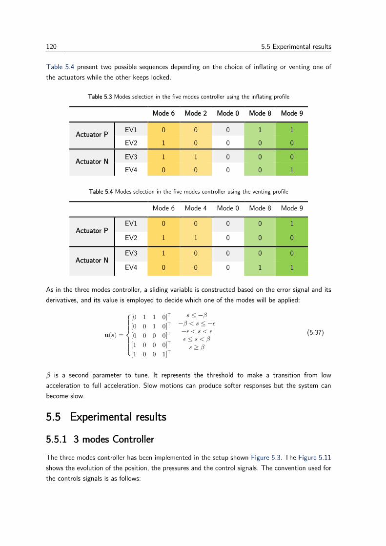
120 5.5 Experimental results

Table 5.4 present two possible sequences depending on the choice of inflating or venting one of

the actuators while the other keeps locked.

Table 5.3 Modes selection in the five modes controller using the inflating profile

Mode 6 Mode 2 Mode 0 Mode 8 Mode 9

Actuator P EV1 0 0 0 1 1

EV2 1 0 0 0 0

Actuator N EV3 1 1 0 0 0

EV4 0 0 0 0 1

Table 5.4 Modes selection in the five modes controller using the venting profile

Mode 6 Mode 4 Mode 0 Mode 8 Mode 9

Actuator P EV1 0 0 0 0 1

EV2 1 1 0 0 0

Actuator N EV3 1 0 0 0 0

EV4 0 0 0 1 1

As in the three modes controller, a sliding variable is constructed based on the error signal and its

derivatives, and its value is employed to decide which one of the modes will be applied:

𝐮(𝑠) =

{

[0 1 1 0]⊺

[0 0 1 0]⊺

[0 0 0 0]⊺

[1 0 0 0]⊺

[1 0 0 1]⊺

𝑠 ≤ −𝛽

−𝛽 < 𝑠 ≤ −𝜖−𝜖 < 𝑠 < 𝜖𝜖 ≤ 𝑠 < 𝛽

𝑠 ≥ 𝛽

(5.37)

𝛽 is a second parameter to tune. It represents the threshold to make a transition from low

acceleration to full acceleration. Slow motions can produce softer responses but the system can

become slow.

5.5 Experimental results

5.5.1 3 modes Controller

The three modes controller has been implemented in the setup shown Figure 5.3. The Figure 5.11

shows the evolution of the position, the pressures and the control signals. The convention used for

the controls signals is as follows:

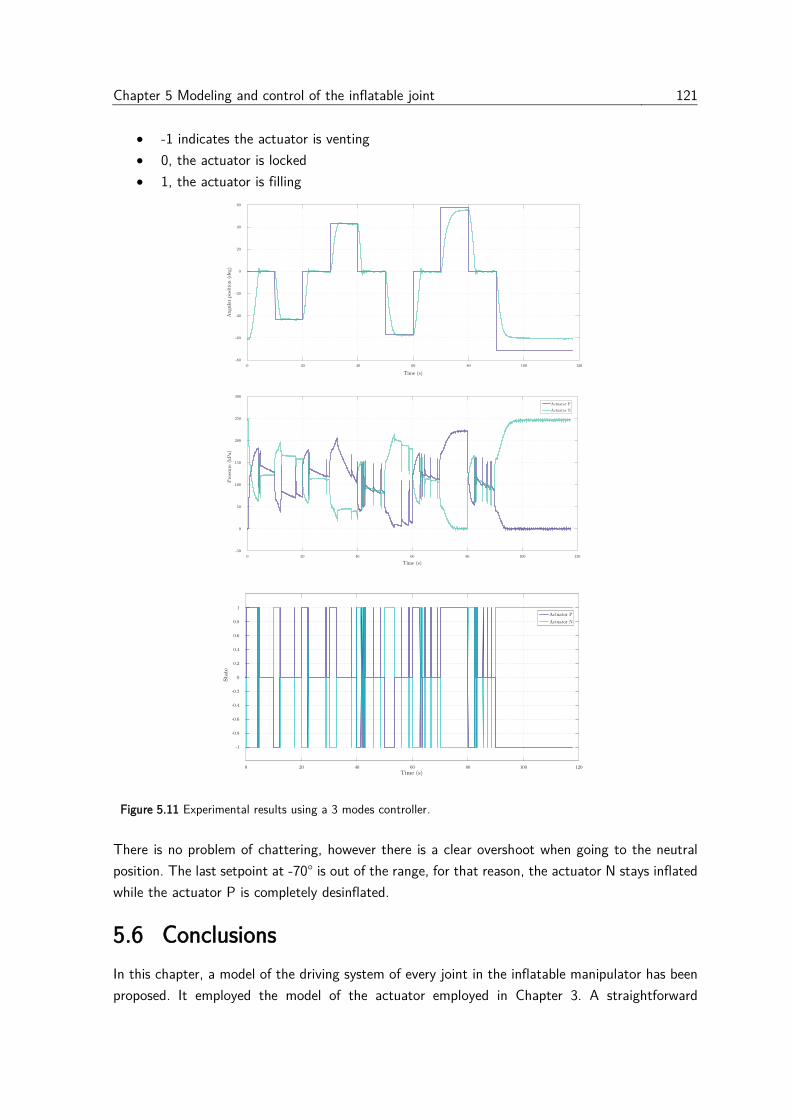
Chapter 5 Modeling and control of the inflatable joint 121

• -1 indicates the actuator is venting

• 0, the actuator is locked

• 1, the actuator is filling

Figure 5.11 Experimental results using a 3 modes controller.

There is no problem of chattering, however there is a clear overshoot when going to the neutral

position. The last setpoint at -70° is out of the range, for that reason, the actuator N stays inflated

while the actuator P is completely desinflated.

5.6 Conclusions

In this chapter, a model of the driving system of every joint in the inflatable manipulator has been

proposed. It employed the model of the actuator employed in Chapter 3. A straightforward

122 5.6 Conclusions

approach was proposed, through the implementation and validation of an existing control strategy

based on sliding mode control. The different control structures were validated in a mockup using

a rigid disc and a prototype of the inflatable joint. The results show that the implemented strategy

is effective and robust in spite of their simplicity.

Chapter 6

Conclusions

The discipline of writing something down is the

first step toward making it happen

― Lee Lacocca

Contents

6.1 Conclusions .....................................................................................................123

6.1.1 Analysis, modelling, and characterization of inflatable actuators based on

simultaneous eversion and retraction .................................................................... 124

6.1.2 Development of a shape sensing means for deformable structures ............... 125

6.1.3 Position control of an inflatable joint ......................................................... 125

6.2 Perspectives ....................................................................................................126

6.2.1 Structure .................................................................................................. 126

6.2.2 Actuator ................................................................................................... 126

6.2.3 Sensor ...................................................................................................... 127

6.2.4 Control ..................................................................................................... 128

6.1 Conclusions

Soft robotics is a field in full development and expansion. Although most of the attention is

currently addressed to soft robots made of elastomers, another promising field is related to

inflatable robots. Their intrinsic lightness and compliance make them suitable candidates for

applications where safe interaction with the environment is capital, such as human-robot

collaboration, robotic manipulation or the inspection of hazardous environments. Furthermore, an

inflatable structure can be folded and packed efficiently, easing its transportation and deployment,

124 6.1 Conclusions

which is a feature almost unique in robotics. However, it also supposes that conventional strategies

of actuation, sensing, modeling, and control require to be adapted to the particular conditions of

inflatable bodies, namely, lightness and deformability. This thesis falls within the scope of the

control of a long-range arm whose structure and actuation are entirely inflatable. Different axes of

research were explored:

• The analysis, modeling, and characterization of inflatable actuators based on simultaneous

eversion and retraction.

• The proposition and development of a shape sensing means for deformable structures,

based on the implementation of a distributed network of MARG sensors.

• The control strategy of the position of an inflatable joint.

Although the primary objective concerning the position control of the end effector is not completely

met yet, this work constitutes a solid base for bringing inflatable robots from research laboratories

to real situations and spread their utilization in a wide range of new applications beyond their

pertinence in the nuclear field.

6.1.1 Analysis, modelling, and characterization of inflatable

actuators based on simultaneous eversion and retraction

We analyzed a new concept of inflatable actuator based on the principle of simultaneous eversion

and retraction. Two different geometries were considered: cylindrical and conical. In both cases,

we showed that the total stroke is almost twice the initial length, and the force developed is well

distributed through a great portion of the stroke. Both features represent true strengths in contrast

with the most common pneumatic artificial muscles, whose stroke is only a portion of the initial

length, and the force decreases severely with the contraction.

We developed a simple model of the force based on a static and geometric analysis, and we

contrasted it with experimental data. We showed that the model developed is representative of the

behavior, however as it lacks of other considerations concerning the envelope material or the

boundary conditions, the predicted force diverges in the regions close to the actuator limits. The

use of exponential contact laws enhanced the model, but it remains specific to a particular

experimental case, and we could not go further in its evaluation with other prototypes. Instead, we

proposed a more accurate model approach by means of finite elements analysis. The proposed

framework goes from the parametric generation of the geometry to the FE model simulation. In

contrast to the analytical model, simulation results showed, close to the stroke limits, good

agreement of the developed force with experimental data. Furthermore, it reproduced the apparition

of folds and wrinkles whose effects were not considered in the previous analysis. However, further

development is needed to obtain a nominal model that reproduces the behavior in the integrity of

the stroke and not only at its boundaries.

Chapter 6 Conclusions 125

6.1.2 Development of a shape sensing means for deformable

structures

We proposed and implemented a method to estimate the configuration of the inflatable arm. The

approach is based on the utilization of a distributed network of MARG sensors through the entire

arm. This solution responds to different requirements involving lightness, adaptability to deformable

structures, and low cost.

The first stage exploiting sensor data addressed the utilization of permanent magnets perturbing

magnetometers, and the estimation of the relative angular position between two segments of the

arm based on the variation of the measured magnetic field. We could show that under controlled

conditions, the estimation converges to the real measure. Moreover, the fusion of the three available

measures from the magnetometer aims to provide an estimate more robust to different kinds of

perturbations. Experiments in a prototype of the inflatable joint confirmed that the use of three

measures provided an estimate more precise than using only one of the inputs. However, those

tests also showed that the surfaces where the magnet and the sensor are attached, can suffer from

deformations, and they have an essential effect the proposed method is not robust to.

The second stage proposed the fusion of the rest of the available measures, namely, the readings

coming from the accelerometers and gyroscopes. The approach is based on the utilization of

quaternions as an efficient representation of solid rotations. The generalization of an existing

method to estimate an orientation from a minimal set of vector observations was introduced.

Thereafter, it allowed establishing the relative orientation between two mobile frames directly,

without requiring a fixed reference frame. Simultaneously, intending to exploit the gyroscopes

measures, another development drove to a relationship between the relative rotation between two

mobile frames and their rotation velocity. This approach was validated through simulation. It needs

to be tested in a real situation.

6.1.3 Position control of an inflatable joint

The model of the inflatable actuator, as well as the method of the relative orientation between two

segments of the robot, are the bricks to propose the position control of every joint of the inflatable

arm. A straightforward approach was proposed, through the implementation and validation of a

control strategy based on sliding mode control. The different control structures demonstrated to

be effective and robust in spite of their simplicity.

With the aim to overcome the problem of non-colocalization between the pressure sensors and the

actuators, an observer was proposed. It will be useful in the implementation of more complex

control structures that need full knowledge of the state to control the position and the stiffness of

the joint.

126 6.2 Perspectives

6.2 Perspectives

Soft robotics looks for adapting robotics towards more natural interactions, which involves

rethinking every aspect of a robotic device, from the hardware side, actuation, sensing and

transmission of data and power, to the software part, including the modeling of deformable bodies,

the identification techniques as well as the control strategies. The path to go through is still long

but surely exciting. Soft robotics will continue to gather people from transverse (apparently

disjoined) domains, as engineers, mathematicians, biologists, chemists, architects, designers, to

work around a common goal: learn from nature to imagine and create more natural robots.

6.2.1 Structure

The structure could be redesigned introducing an arborescent shape instead of a single serial chain.

Such a structure would take advantage of its compliance and take support on the environment

without the risk of damage. This idea has already been proposed in (Lastinger et al., 2019) and

the novelty would reside in the completely inflatable feature.

Flexible electronics is an active research field. One could think about embedding the circuits and

sensors in the fabric that delimits the structure or even the actuators. It could enable the direct

integration of pressure sensors in the actuators and avoid the problem of non-colocation; or even

the integration of other kinds of sensors in the structure, to measure proximity, strain or

temperature, without adding lots of additional cables. It allows us to imagine the creation of a

complex “skin and nervous system”, making an analogy with the human body.

6.2.2 Actuator

Further experimental campaigns in the characterization of the material could be carried out to

have a better estimation of its properties. It would be suitable to use specialized equipment for

tissue characterization, such as a biaxial testing machine. Other experimental tests could be carried

out to determine the resistance to fatigue and the lifespan of the actuator.

The refinement of the finite elements model will be a key step to pursue multiple developments:

by modifying the properties of the elements on the edges, the behavior of the sewing could be

taken into account in order to analyze their effect in the stress concentration. Another axis of

development is the optimization of the shape: as it was introduced in the actuator description, the

curve that generates the volume is required to be monotonically increasing. We have explored

constant and linear curves, but other shapes could be explored to improve the force-displacement

characteristic. The study of the geometry of the rear surface, joining the actuator tip to the major

surface, has been skipped in this work, but it plays a critical role, for instance, in the shape

determination of the rear cross-section when the actuator is inflated completely.

Chapter 6 Conclusions 127

The finite elements model will also be useful in simulations of the entire antagonistic system, in

order to optimize the positioning and attachment of the actuators, their interaction with the

structure, and would be the framework to test other control strategies in simulation.

Although the geometry generation of the actuator has been automatized, it remains approximative.

The process of obtaining flat panels and how they must be interconnected to get the desired shape

when inflated, is not a trivial problem. Further work could be based in (Skouras et al., 2014) to

obtain flat patterns from a 3D model of the desired inflated shape. Another interesting approach

could be based on the utilization of new computational techniques to generate knitted surfaces

from 3D models (Vidya Narayanan, 2018). It could lead to the fabrication of actuators without

sewings, avoiding the stress concentration.

6.2.3 Sensor

Concerning the strategy using permanent magnets as more reliable magnetic sources, future work

could be steered in three directions:

The first one could consider the utilization of more sensors, which would raise more information

and improve the robustness of the proposed approach. An interesting method is described in

(Kortier et al., 2015). The authors made use of a constellation of multiple magnetometers

perturbed by a mobile permanent magnet that had also attached an inertial sensor. The study

aimed to estimate the relative pose of a user’s hand (where the permanent magnet was attached),

and his trunk (which supported the sensor constellation) and showed good results of the estimation

of position and orientation of the hand.

The second direction could be focused on the implementation of alternatives to the mapping

between magnetic fields readings and angular position. Here we proposed a simple method based

on a gradient descent algorithm, but other approaches can be explored such as neural networks or

machine learning techniques, which can tackle measures subjected to hysteresis phenomena in a

better way. For instance, (Han et al., 2018) proposed a recurrent neural network for estimating

the magnitude and the location of contact pressure in a microfluidic soft sensor, which also

presented hysteretic behavior.

The third direction would explore other arrangements of magnets in order to focalize the magnetic

field in a better way, for instance, the Halbach array (Halbach, 1981) that increases the magnetic

field on one side of the array while canceling the field near to zero on the other side.

In the other hand, the second approach proposing the fusion of measures from two consecutive

MARG sensors needs to be validated experimentally. It is plausible that, as in the first case, the

rotation estimate does not follow the trajectory of a perfect revolute joint. To overcome this

problem, advanced processing techniques of quaternions could be implemented, such as quaternion

filtering or geodesic projection.

Further developments could be focused on the calibration of the sensor to body relative orientation.

Our work focused on orientation estimation but position estimation could also be considered. The

128 6.2 Perspectives

main problem of position estimation using inertial sensors is the time drift, due to the double

integration of noisy signals. However, given that the sensors are attached to the links of a serial

chain instead of being free-floating, several kinematic constraints are introduced, which could be

exploited jointly with the geometrical and kinematic model of the robot, to get an estimation robust

to dynamical effects. (Kok et al., 2014; Laidig et al., 2017) present the principle of this approach.

Finally, the proliferation of fiber optic sensors applications could lead to a cost reduction and

become an affordable solution for shape sensing systems. It would be an important step in the

development of an inspection arm immune to electromagnetic fields and maybe, ionizing radiation.

6.2.4 Control

There are multiple directions to address future work

The estimation of the pressure could lead to the implementation of control strategies to control

the pressure in every actuator and construct a controller capable of guaranteeing a position and

an estimated stiffness simultaneously. This would be the basis to force control techniques applied

to inflatable robotics.

The pressure estimator could be a tool towards the development of techniques for the detection

and quantification of leakages in the actuators, which is a crucial step to implement fault-tolerant

control techniques and guarantee the integrity and operation of the entire robot until the end of

the task. A first approach could be inspired by (Wilson et al., 2017), where authors proposed

adapting the stiffness of an inflatable joint to reduce the mass flow rate of the leak.

The development of a static model of the entire structure, taking into account the joint limits and

stiffness, as well as the buckling limit of the links, would be a first step to the synthesis of trajectory

path planning strategies, guaranteeing the stability of the whole structure.

Finally, the employment of the measures issued from accelerometers could lead to perform dynamic

analysis of the structure, with the aim to introduce control strategies to damp vibratory effects.

Appendix A

Rigid body rotation

In this section, we present the mathematical notations referring to the rotations in the space of

rigid bodies, and the most common representations of rotations, giving a deeper insight into the

theory of quaternions.

A rotation is a displacement in which at least one point of a rigid body remains in its initial position

and not all lines in the body remain parallel to their initial orientations.

Consider an orthonormal frame of reference 𝐹𝑅. The unit vectors 𝐱, 𝐲, 𝐳 are the frame axes.

Consider a free rigid body and another orthonormal frame 𝐹𝐵 attached to it, with unit vectors 𝐱′,

𝐲′, 𝐳′ as frame axes. These vectors can be expressed as linear combinations of the vectors of the

reference frame:

𝐱′ = 𝑥𝑥′ 𝐱 + 𝑥𝑦

′ 𝐲 + 𝑥𝑧′ 𝐳

𝐲′ = 𝑦𝑥′ 𝐱 + 𝑦𝑦

′𝐲 + 𝑦𝑧′𝐳

𝐳′ = 𝑧𝑥′ 𝐱 + 𝑧𝑦

′𝐲 + 𝑧𝑧′𝐳

(A.1)

Where the scalars 𝑥𝑖′, 𝑦𝑖′, 𝑧𝑖′ 𝑖 ∈ {𝑥, 𝑦, 𝑧} are the direction cosines of the axes of the frame 𝐹𝐵 with

respect to the reference frame 𝐹𝑅.

A.1 Rotation matrix

The expression (A.1) can be written in a more compact form stacking the vectors 𝐱′, 𝐲′, 𝐳′ as the

columns of a matrix 𝑅, termed rotation matrix:

𝑅 = [𝐱′ 𝐲′ 𝐳′] =

[ 𝑥𝑥′ 𝑦𝑥

′ 𝑧𝑥′

𝑥𝑦′ 𝑦𝑦

′ 𝑧𝑦′

𝑥𝑧′ 𝑦𝑧

′ 𝑧𝑧′] =

[ 𝐱′ ⋅ 𝐱 𝐲′ ⋅ 𝐱 𝐳′ ⋅ 𝐱

𝐱′ ⋅ 𝐲 𝐲′ ⋅ 𝐲 𝐳′ ⋅ 𝐲

𝐱′ ⋅ 𝐳 𝐲′ ⋅ 𝐳 𝐳′ ⋅ 𝐲] (A.2)

130 A.2 Euler angles

Given that vectors 𝐱′, 𝐲′, 𝐳′ are mutually orthonormal, the columns of the matrix 𝑅 (denoted here

as 𝑟1, 𝑟2,𝑟3) are too. It follows that

𝑟𝑖⊺𝑟𝑗 = {

0, 𝑖 ≠ 𝑗

1, 𝑖 = 𝑗 (A.3)

This property can be written as

𝑅𝑅⊺ = 𝑅⊺𝑅 = 𝐼3 (A.4)

From this, it follows

𝑑𝑒𝑡(𝑅) = ±1 (A.5)

If the frame is right-handed, the determinant is equal to +1. The set of all 3 × 3 matrices which

satisfy the property in (A.4), and det(𝑅) = +1 is denoted 𝑆𝑂(3). (𝑆𝑂 for Special Orthogonal;

special refers to the fact that det(𝑅) = +1).

Rotation matrix has three geometrical meanings (Sciavicco and Siciliano, 2000):

• It describes the mutual orientation between two frames; its column vectors are the

direction cosines of the axes of the rotating frame with respect to the original frame.

• It represents the coordinate transformation between the coordinates of a point expressed

in two different frames.

• It is the operator that allows rotating a vector in the same frame.

Considering rotation matrix as an operator, elementary rotations can be obtained by rotating about

any of the principal axes 𝑥, 𝑦 or 𝑧 through an angle 𝜃:

𝑅𝑥(𝜃) = [1 0 00 cos 𝜃 − sin 𝜃0 sin 𝜃 cos 𝜃

]

𝑅𝑦(𝜃) = [cos 𝜃 0 sin 𝜃0 1 0

− sin 𝜃 0 cos 𝜃

]

𝑅𝑧(𝜃) = [cos 𝜃 − sin 𝜃 0sin 𝜃 cos 𝜃 00 0 1

]

(A.6)

The main drawback of the rotation matrix is their superabundance, they have nine scalars but the

condition of orthogonality introduces six constraints among them, so they are not independent. It

follows that three parameters would be sufficient to describe the orientation of a body. This fact

motivated other representations of rotations in terms of a reduced number of parameters.

A.2 Euler angles

This representation consists of describing the orientation of a frame respect to a fixed reference as

a sequence of three elementary rotations while guaranteeing that two successive rotations are not

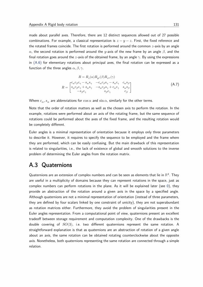
Appendix A Rigid body rotation 131

made about parallel axes. Therefore, there are 12 distinct sequences allowed out of 27 possible

combinations. For example, a classical representation is 𝑧 − 𝑦 − 𝑧. First, the fixed reference and

the rotated frames coincide. The first rotation is performed around the common 𝑧-axis by an angle

𝛼, the second rotation is performed around the 𝑦-axis of the new frame by an angle 𝛽, and the

final rotation goes around the 𝑧-axis of the obtained frame, by an angle 𝛾. By using the expressions

in (A.6) for elementary rotations about principal axes, the final rotation can be expressed as a

function of the three angles 𝛼, 𝛽, 𝛾.

𝑅 = 𝑅𝑧(𝛼)𝑅𝑦′(𝛽)𝑅𝑧′′(𝛾)

𝑅 = [

𝑐𝛼𝑐𝛽𝑐𝛾 − 𝑠𝛼𝑠𝛾 −𝑐𝛼𝑐𝛽𝑠𝛾 − 𝑠𝛼𝑐𝛾 𝑐𝛼𝑠𝛽𝑠𝛼𝑐𝛽𝑐𝛾 + 𝑠𝛼𝑠𝛾 −𝑠𝛼𝑐𝛽𝑠𝛾 + 𝑐𝛼𝑐𝛾 𝑠𝛼𝑠𝛽−𝑠𝛽𝑐𝛾 𝑠𝛽𝑐𝛾 𝑐𝛽

] (A.7)

Where 𝑐𝛼, 𝑠𝛼 are abbreviations for cos 𝛼 and sin 𝛼, similarly for the other terms.

Note that the order of rotation matters as well as the chosen axis to perform the rotation. In the

example, rotations were performed about an axis of the rotating frame, but the same sequence of

rotations could be performed about the axes of the fixed frame, and the resulting rotation would

be completely different.

Euler angles is a minimal representation of orientation because it employs only three parameters

to describe it. However, it requires to specify the sequence to be employed and the frame where

they are performed, which can be easily confusing. But the main drawback of this representation

is related to singularities, i.e., the lack of existence of global and smooth solutions to the inverse

problem of determining the Euler angles from the rotation matrix.

A.3 Quaternions

Quaternions are an extension of complex numbers and can be seen as elements that lie in ℝ4. They

are useful in a multiplicity of domains because they can represent rotations in the space, just as

complex numbers can perform rotations in the plane. As it will be explained later (see 0), they

provide an abstraction of the rotation around a given axis in the space by a specified angle.

Although quaternions are not a minimal representation of orientation (instead of three parameters,

they are defined by four scalars linked by one constraint of unicity), they are not superabundant

as rotation matrices either. Furthermore, they avoid the problem of singularities present in the

Euler angles representation. From a computational point of view, quaternions present an excellent

tradeoff between storage requirement and computation complexity. One of the drawbacks is the

double covering of 𝑆𝑂(3), i.e. two different quaternions represent the same rotation. A

straightforward explanation is that as quaternions are an abstraction of rotation of a given angle

about an axis, the same rotation can be obtained rotating counterclockwise about the opposite

axis. Nonetheless, both quaternions representing the same rotation are connected through a simple

relation.

132 A.3 Quaternions

Here, we intend to give some of the main concepts of quaternions properties and operations that

will be useful in further analysis. For a more in-depth description of this mathematical tool, the

reader is invited to refer to (Kuipers, 2002).

A.3.1 History and definition

William Rohan Hamilton introduced quaternions in XIX century. He was fascinated by the role that

complex numbers have as rotation operators in the plane. He wanted to find something equivalent

to represent rotations in the space. For years, he tried to invent an algebra of “triplets”, without

success. In 1843, he discovered that the answer was a four-dimension division algebra that he called

quaternions. From 1843 to 1850 he published 18 instalments in the Philosophical Magazine,

describing his work about quaternions (Hamilton, 1844).

Quaternions are considered as an extension of complex numbers. A quaternion has the following

form:

𝑞 = 𝑞0 + 𝑞1𝑖 + 𝑞2𝑗 + 𝑞3𝑘 ≡ 𝑞0 + 𝒒 (A.8)

where 𝑞0, 𝑞1, 𝑞2 and 𝑞3 are real quantities denoted as the components of the quaternion 𝑞, and

also called Euler parameters; 𝑖, 𝑗, and 𝑘 are linearly independent imaginary units, satisfying the

following combinatory rules:

𝑖 ⋅ 𝑖 = 𝑗 ⋅ 𝑗 = 𝑘 ⋅ 𝑘 = −1

𝑖 ⋅ 𝑗 = 𝑘, 𝑗 ⋅ 𝑘 = 𝑖, 𝑘 ⋅ 𝑖 = 𝑗

𝑗 ⋅ 𝑖 = −𝑘, 𝑘 ⋅ 𝑗 = −𝑖, 𝑖 ⋅ 𝑘 = −𝑗

(A.9)

A common notation of quaternions is the vector form as proposed in the right hand of (A.8), where

𝑞0 is called the scalar part and 𝑞1, 𝑞2, 𝑞3 are grouped as the components of a vector 𝐪 in ℝ3. This

notation will be useful when considering the geometrical interpretation of the action of quaternions.

Note that any vector 𝐩 ∈ ℝ3 can be represented as a quaternion with a null scalar part. Quaternions

with the scalar part equal to zero are called pure quaternions.

A.3.2 Relations and Operations

A.3.2.1 Equality and Addition

Given two quaternions 𝑢 and 𝑣:

𝑢 = 𝑢0 + 𝑢1𝑖 + 𝑢2𝑗 + 𝑢3𝑘

𝑣 = 𝑣0 + 𝑣1𝑖 + 𝑣2𝑗 + 𝑣3𝑘

They are said to be equal if and only if

𝑢0 = 𝑣0 𝑢1 = 𝑣1 𝑢2 = 𝑣2 𝑢3 = 𝑣3

Appendix A Rigid body rotation 133

The addition of their corresponding components defines the sum of two quaternions:

𝑢 + 𝑣 = (𝑢0 + 𝑣0) + (𝑢1 + 𝑣1)𝑖 + (𝑢2 + 𝑣2)𝑗 + (𝑢3 + 𝑣3)𝑘 (A.10)

The sum of two quaternions results in another quaternion. Moreover, addition is commutative and

associative. There exists a zero quaternion (𝟎) that added to any other quaternion results in the

same quaternion. Likewise, for any quaternion there exists a negative quaternion such that the

addition of both of them gives the zero quaternion:

𝑞 + 𝟎 = 𝑞

𝑞 + (−𝑞) = 𝟎

with

𝟎 = 0 + 0𝑖 + 0𝑗 + 0𝑘 = 0 + 𝟎

−𝑞 = −𝑞0 − 𝑞1𝑖 − 𝑞2𝑗 − 𝑞3𝑘 ≡ −𝑞0 − 𝐪

A.3.2.2 Product

The product of a quaternion 𝑞 by a scalar 𝑐 is defined in the same manner as in ℝ3: every

component of the quaternion is multiplied by the scalar 𝑐. The product of two quaternions considers

the relations introduced in (A.9). Consider again two quaternions 𝑢 and 𝑣 as denoted above. Their

product is developed as follows:

𝑢 ⋅ 𝑣 = (𝑢0 + 𝑢1𝑖 + 𝑢2𝑗 + 𝑢3𝑘) ⋅ (𝑣0 + 𝑣1𝑖 + 𝑣2𝑗 + 𝑣3𝑘)

(A.11)

= (𝑢0𝑣0 − 𝑢1𝑣1 − 𝑢2𝑣2 − 𝑢3𝑣3) +

(𝑢0𝑣1 + 𝑢1𝑣0 + 𝑢2𝑣3 − 𝑢3𝑣2)𝑖 +

(𝑢0𝑣2 − 𝑢1𝑣3 + 𝑢2𝑣0 + 𝑢3𝑣1)𝑗 +

(𝑢0𝑣3 + 𝑢1𝑣2 − 𝑢2𝑣1 + 𝑢3𝑣0)𝑘

The product of two quaternions results in another quaternion. It holds the associative property,

but contrary to addition, it is not commutative. There exists an identity quaternion (𝟏) satisfying

that the product of any quaternion with it returns the same quaternion:

𝑞 ⋅ 𝟏 = 𝟏 ⋅ 𝑞 = 𝑞

with

𝟏:= 1 + 0𝑖 + 0𝑗 + 0𝑘 = 1 + 𝟎

Quaternions can also be expressed as tuples of four elements, and the product (A.11) can be

written using the algebra of matrices. Let 𝑤 be the quaternion obtained from the product 𝑢 ⋅ 𝑣:

𝑤 = 𝑢 ⋅ 𝑣 = 𝑤0 +𝑤1𝑖 + 𝑤2𝑗 + 𝑤3𝑘

𝑤 can be rewritten in a matrix form as:

134 A.3 Quaternions

𝑤 = [𝑢]𝐿𝑣

[

𝑤0𝑤1𝑤2𝑤3]

=

[

𝑢0 −𝑢1 −𝑢2 −𝑢3𝑢1 𝑢0 −𝑢3 𝑢2𝑢2 𝑢3 𝑢0 −𝑢1𝑢3 −𝑢2 𝑢1 𝑢0]

[

𝑣0𝑣1𝑣2𝑣3]

= [𝑢0 −𝐮⊺

𝐮 𝑢0𝐼3 + [𝐮]×] 𝑣 (A.12)

Where 𝐼3 is the identity matrix of size 3, and [𝐮]× is the skew-symmetric matrix representing the

cross product of vector 𝐮:

𝐮 × 𝐯 = [𝐮]×𝐯 =

[ 0 −𝑢3 𝑢2𝑢3 0 −𝑢1−𝑢2 𝑢1 0 ]

[

𝑣1𝑣2𝑣3

] (A.13)

Given that quaternion product is non-commutative, it is important to clarify the order of operands:

sub-index 𝐿 in [𝑢]𝐿 means that it is the matrix representation of the quaternion product of 𝑢 on

the left of 𝑣. Another matrix can be obtained for the product on the right:

𝑤 = [𝑣]𝑅𝑢

[

𝑤0𝑤1𝑤2𝑤3]

=

[

𝑣0 −𝑣1 −𝑣2 −𝑣3𝑣1 𝑣0 𝑣3 −𝑣2𝑣2 −𝑣3 𝑣0 𝑣1𝑣3 𝑣2 −𝑣1 𝑣0]

[

𝑢0𝑢1𝑢2𝑢3]

= [𝑣0 −𝐯⊺

𝐯 𝑣0𝐼3 + [𝐯]×⊺] 𝑢 (A.14)

[𝑣]𝑅 is the matrix representation of the quaternion product of 𝑣 on the right of 𝑢.

In the vector form, it can be demonstrated that the product of two quaternions is obtained as:

𝑢 ⋅ 𝑣 = (𝑢0𝑣0 − 𝐮 ⋅ 𝐯) + (𝑢0𝐯 + 𝑣0𝐮 + 𝐮 × 𝐯) (A.15)

Where operators (⋅) and (×) are respectively the dot and cross product of vectors in ℝ3.

A.3.2.3 Complex Conjugate

In the same manner, as complex numbers have conjugate, it is also defined for quaternions. Given

a quaternion

𝑞 = 𝑞0 + 𝑞1𝑖 + 𝑞2𝑗 + 𝑞3𝑘

The complex conjugate of 𝑞, denoted 𝑞∗, is defined as

𝑞∗ = 𝑞 = 𝑞0 − 𝑞1𝑖 − 𝑞2𝑗 − 𝑞3𝑘 = 𝑞0 − 𝐪 (A.16)

It can be demonstrated that the conjugate of the quaternion product is equal to the product of

the individual conjugates in reverse order:

(𝑢 ⋅ 𝑣) = 𝑣∗ ⋅ 𝑢∗ (A.17)

Appendix A Rigid body rotation 135

A.3.2.4 Norm

We can define a norm for quaternions, in the same manner as for complex numbers. The norm of

a quaternion 𝑞, is a scalar denoted ‖𝑞‖, defined as:

‖𝑞‖ = √𝑞∗ ⋅ 𝑞 = √𝑞02 + 𝑞1

2 + 𝑞22 + 𝑞3

2 (A.18)

Quaternions whose norm is equal to 1 are called unit or normalized quaternions.

The norm of the product of two quaternions is equal to the product of their norms:

‖𝑢 ⋅ 𝑣‖ = ‖𝑢‖‖𝑣‖ (A.19)

A.3.2.5 Inverse

Any quaternion 𝑞 (different to the zero quaternion) has an inverse: another quaternion denoted

𝑞−1, such that their product in any order is equal to the identity quaternion.

𝑞 ⋅ 𝑞−1 = 𝑞−1 ⋅ 𝑞 = 𝟏

𝑞−1 can be computed as:

𝑞−1 =𝑞∗

‖𝑞‖2 (A.20)

Note that if 𝑞 is a unit quaternion, its conjugate is also its inverse.

A.3.2.6 Quaternion square root

The square root of a quaternion 𝑞 is defined as the quaternion 𝑤 that satisfies the following

equation:

𝑤2 = 𝑤 ⋅ 𝑤 = 𝑞 (A.21)

From the quaternion product, a set of four nonlinear equations are obtained, with the four

components of 𝑤 as unknowns:

𝑤02 − 𝑤1

2 −𝑤22 − 𝑤3

2 = 𝑞0

2𝑤0𝑤1 = 𝑞1

2𝑤0𝑤2 = 𝑞2

2𝑤0𝑤3 = 𝑞3

If 𝑞 is a unit quaternion, it implies that 𝑤 is also a unit quaternion. In that case, the equations can

be simplified, and a closed solution is obtained:

136 A.3 Quaternions

[

𝑤0𝑤1𝑤2𝑤3]

=

1

√2(𝑞0 + 1)[

𝑞0 + 1𝑞1𝑞2𝑞3 ]

(A.22)

Moreover, by developing the term in the square root, it can be found that it corresponds to the

norm of the quaternion in the right-hand side:

2(𝑞0 + 1) = 2𝑞0 + 2

= 2𝑞0 + 1 + 𝑞02 + 𝑞1

2 + 𝑞22 + 𝑞3

2

= (𝑞0 + 1)2 + 𝑞1

2 + 𝑞22 + 𝑞3

2

From this last observation, the square root of a unit quaternion can be written in a compact form:

𝑞1 2⁄ =𝑞 + 𝟏

‖𝑞 + 𝟏‖ (A.23)

The square root of a unit quaternion has an interesting geometrical interpretation that will be

explained soon (see A.3.3.1).

A.3.2.7 Quaternion adjoint operator

The adjoint operator of a unit quaternion 𝑞 is a transformation that takes a vector 𝐱 ∈ ℝ3 and

transforms it into another vector:

𝐴𝑑𝑞: ℝ3 → ℝ3 𝒙 ↦ 𝑞 ⋅ 𝑥 ⋅ 𝑞−1 (A.24)

The adjoint operator holds the following properties:

Linearity: For any two vectors 𝐮, 𝐯 ∈ ℝ3 and any scalar 𝑐 ∈ ℝ:

Ad𝑞(𝐮 + c𝐯) = Ad𝑞(𝐮) + cAd𝑞(𝐯)

Norm invariance: For any vector 𝐮 ∈ ℝ3, its norm is invariant under the application of the adjoint

operator:

‖Ad𝑞(𝐮)‖ = ‖𝐮‖

A.3.3 Unit quaternions as rotation operators

At this point, the main operations and properties of quaternions have been presented. As we said

at the beginning of this section, the interest on quaternions (and more precisely unit quaternions)

is related to their capacity to represent rotations in the space. The demonstration of the following

theorem is out of the scope of this text; the reader can refer to (Kuipers, 2002) for more details.

Theorem: Given a vector 𝐩 ∈ ℝ3 and a unit quaternion 𝑞 with the form

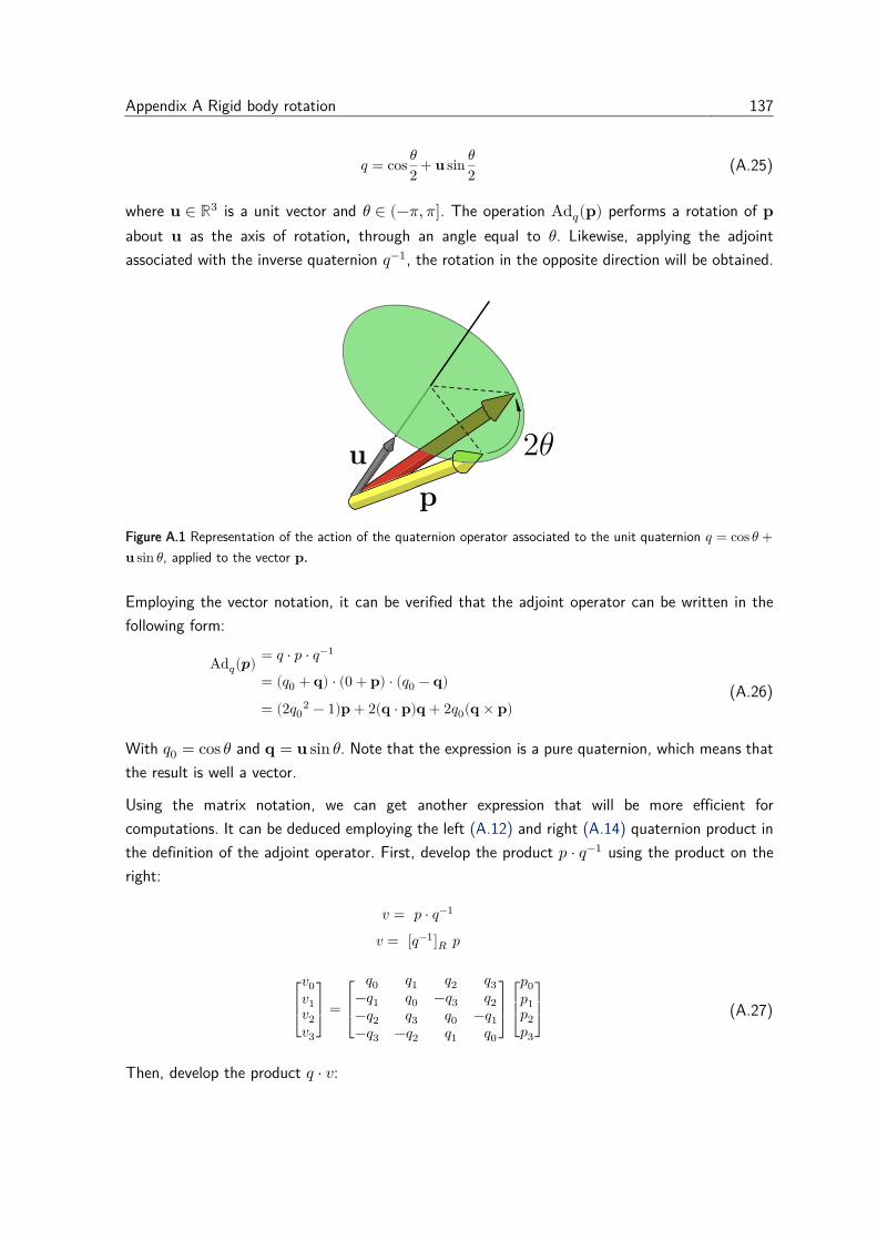
Appendix A Rigid body rotation 137

𝑞 = cos𝜃

2+ 𝐮 sin

𝜃

2 (A.25)

where 𝐮 ∈ ℝ3 is a unit vector and 𝜃 ∈ (−𝜋, 𝜋]. The operation Ad𝑞(𝐩) performs a rotation of 𝐩

about 𝐮 as the axis of rotation, through an angle equal to 𝜃. Likewise, applying the adjoint

associated with the inverse quaternion 𝑞−1, the rotation in the opposite direction will be obtained.

Figure A.1 Representation of the action of the quaternion operator associated to the unit quaternion 𝑞 = cos 𝜃 +

𝐮 sin 𝜃, applied to the vector 𝐩.

Employing the vector notation, it can be verified that the adjoint operator can be written in the

following form:

Ad𝑞(𝒑) = 𝑞 ⋅ 𝑝 ⋅ 𝑞−1

= (𝑞0 + 𝐪) ⋅ (0 + 𝐩) ⋅ (𝑞0 − 𝐪)

= (2𝑞02 − 1)𝐩 + 2(𝐪 ⋅ 𝐩)𝐪 + 2𝑞0(𝐪 × 𝐩)

(A.26)

With 𝑞0 = cos 𝜃 and 𝐪 = 𝐮 sin 𝜃. Note that the expression is a pure quaternion, which means that

the result is well a vector.

Using the matrix notation, we can get another expression that will be more efficient for

computations. It can be deduced employing the left (A.12) and right (A.14) quaternion product in

the definition of the adjoint operator. First, develop the product 𝑝 ⋅ 𝑞−1 using the product on the

right:

𝑣 = 𝑝 ⋅ 𝑞−1

𝑣 = [𝑞−1]𝑅 𝑝

[

𝑣0𝑣1𝑣2𝑣3]

=

[

𝑞0 𝑞1 𝑞2 𝑞3−𝑞1 𝑞0 −𝑞3 𝑞2−𝑞2 𝑞3 𝑞0 −𝑞1−𝑞3 −𝑞2 𝑞1 𝑞0]

[

𝑝0𝑝1𝑝2𝑝3]

(A.27)

Then, develop the product 𝑞 ⋅ 𝑣:

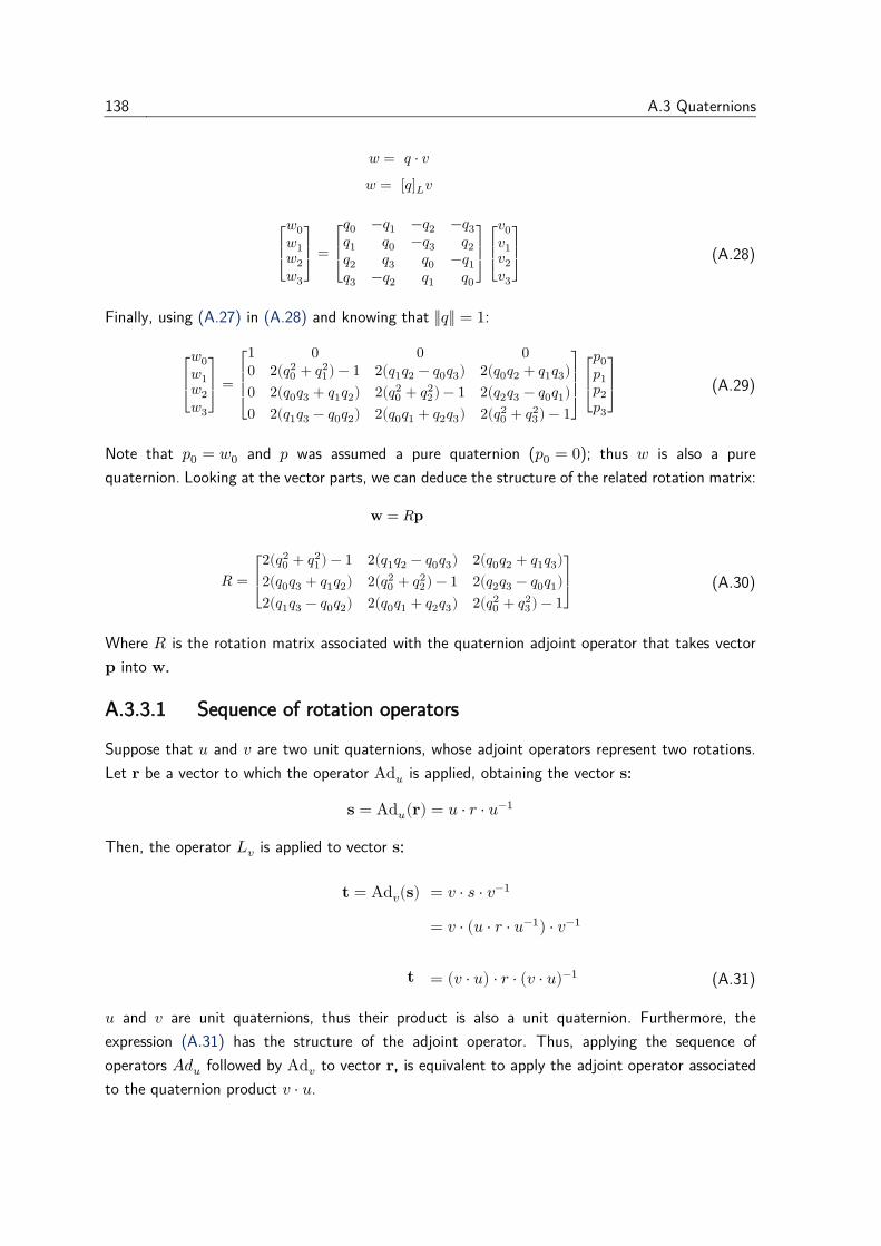
138 A.3 Quaternions

𝑤 = 𝑞 ⋅ 𝑣

𝑤 = [𝑞]𝐿𝑣

[

𝑤0𝑤1𝑤2𝑤3]

=

[

𝑞0 −𝑞1 −𝑞2 −𝑞3𝑞1 𝑞0 −𝑞3 𝑞2𝑞2 𝑞3 𝑞0 −𝑞1𝑞3 −𝑞2 𝑞1 𝑞0]

[

𝑣0𝑣1𝑣2𝑣3]

(A.28)

Finally, using (A.27) in (A.28) and knowing that ‖𝑞‖ = 1:

[

𝑤0𝑤1𝑤2𝑤3]

=

[

1 0 0 00 2(𝑞0

2 + 𝑞12) − 1 2(𝑞1𝑞2 − 𝑞0𝑞3) 2(𝑞0𝑞2 + 𝑞1𝑞3)

0 2(𝑞0𝑞3 + 𝑞1𝑞2) 2(𝑞02 + 𝑞2

2) − 1 2(𝑞2𝑞3 − 𝑞0𝑞1)

0 2(𝑞1𝑞3 − 𝑞0𝑞2) 2(𝑞0𝑞1 + 𝑞2𝑞3) 2(𝑞02 + 𝑞3

2) − 1]

[

𝑝0𝑝1𝑝2𝑝3]

(A.29)

Note that 𝑝0 = 𝑤0 and 𝑝 was assumed a pure quaternion (𝑝0 = 0); thus 𝑤 is also a pure

quaternion. Looking at the vector parts, we can deduce the structure of the related rotation matrix:

𝐰 = 𝑅𝐩

𝑅 =

[

2(𝑞02 + 𝑞1

2) − 1 2(𝑞1𝑞2 − 𝑞0𝑞3) 2(𝑞0𝑞2 + 𝑞1𝑞3)

2(𝑞0𝑞3 + 𝑞1𝑞2) 2(𝑞02 + 𝑞2

2) − 1 2(𝑞2𝑞3 − 𝑞0𝑞1)

2(𝑞1𝑞3 − 𝑞0𝑞2) 2(𝑞0𝑞1 + 𝑞2𝑞3) 2(𝑞02 + 𝑞3

2) − 1]

(A.30)

Where 𝑅 is the rotation matrix associated with the quaternion adjoint operator that takes vector

𝐩 into 𝐰.

A.3.3.1 Sequence of rotation operators

Suppose that 𝑢 and 𝑣 are two unit quaternions, whose adjoint operators represent two rotations.

Let 𝐫 be a vector to which the operator Ad𝑢 is applied, obtaining the vector 𝐬:

𝐬 = Ad𝑢(𝐫) = 𝑢 ⋅ 𝑟 ⋅ 𝑢−1

Then, the operator 𝐿𝑣 is applied to vector 𝐬:

𝐭 = Ad𝑣(𝐬) = 𝑣 ⋅ 𝑠 ⋅ 𝑣−1

= 𝑣 ⋅ (𝑢 ⋅ 𝑟 ⋅ 𝑢−1) ⋅ 𝑣−1

𝐭 = (𝑣 ⋅ 𝑢) ⋅ 𝑟 ⋅ (𝑣 ⋅ 𝑢)−1 (A.31)

𝑢 and 𝑣 are unit quaternions, thus their product is also a unit quaternion. Furthermore, the

expression (A.31) has the structure of the adjoint operator. Thus, applying the sequence of

operators 𝐴𝑑𝑢 followed by Ad𝑣 to vector 𝐫, is equivalent to apply the adjoint operator associated

to the quaternion product 𝑣 ⋅ 𝑢.

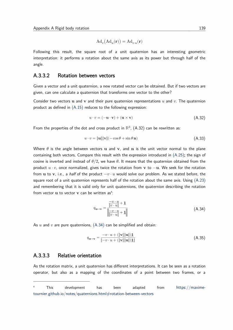
Appendix A Rigid body rotation 139

Ad𝑣(Ad𝑢(𝐫)) = Ad𝑣⋅𝑢(𝐫)

Following this result, the square root of a unit quaternion has an interesting geometric

interpretation: it performs a rotation about the same axis as its power but through half of the

angle.

A.3.3.2 Rotation between vectors

Given a vector and a unit quaternion, a new rotated vector can be obtained. But if two vectors are

given, can one calculate a quaternion that transforms one vector to the other?

Consider two vectors 𝐮 and 𝐯 and their pure quaternion representations 𝑢 and 𝑣. The quaternion

product as defined in (A.15) reduces to the following expression:

𝑢 ⋅ 𝑣 = (−𝐮 ⋅ 𝐯) + (𝐮 × 𝐯) (A.32)

From the properties of the dot and cross product in ℝ3, (A.32) can be rewritten as:

𝑢 ⋅ 𝑣 = ‖𝐮‖‖𝐯‖(− cos 𝜃 + sin 𝜃 𝐧) (A.33)

Where 𝜃 is the angle between vectors 𝐮 and 𝐯, and 𝐧 is the unit vector normal to the plane

containing both vectors. Compare this result with the expression introduced in (A.25); the sign of

cosine is inverted and instead of 𝜃 2⁄ , we have 𝜃. It means that the quaternion obtained from the

product 𝑢 ⋅ 𝑣, once normalized, gives twice the rotation from 𝐯 to −𝐮. We seek for the rotation

from 𝐮 to 𝐯, i.e., a half of the product −𝑣 ⋅ 𝑢 would solve our problem. As we stated before, the

square root of a unit quaternion represents half of the rotation about the same axis. Using (A.23)

and remembering that it is valid only for unit quaternions, the quaternion describing the rotation

from vector 𝐮 to vector 𝐯 can be written as4:

𝑞𝐮↦𝐯 =

−𝑣 ⋅ 𝑢‖𝑣 ⋅ 𝑢‖

+ 𝟏

‖−𝑣 ⋅ 𝑢‖𝑣 ⋅ 𝑢‖

+ 𝟏‖ (A.34)

As 𝑢 and 𝑣 are pure quaternions, (A.34) can be simplified and obtain:

𝑞𝐮↦𝐯 =−𝑣 ⋅ 𝑢 + (‖𝐯‖‖𝐮‖)𝟏

‖−𝑣 ⋅ 𝑢 + (‖𝐯‖‖𝐮‖)𝟏‖ (A.35)

A.3.3.3 Relative orientation

As the rotation matrix, a unit quaternion has different interpretations. It can be seen as a rotation

operator, but also as a mapping of the coordinates of a point between two frames, or a

4 This development has been adapted from https://maxime-

tournier.github.io/notes/quaternions.html#rotation-between-vectors

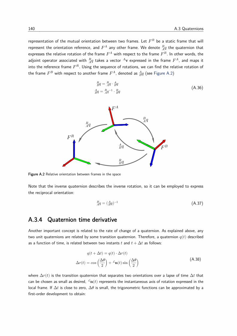
140 A.3 Quaternions

representation of the mutual orientation between two frames. Let 𝐹𝑅 be a static frame that will

represent the orientation reference, and 𝐹𝐴 any other frame. We denote 𝑞𝐴𝑅 the quaternion that

expresses the relative rotation of the frame 𝐹𝐴 with respect to the frame 𝐹𝑅. In other words, the

adjoint operator associated with 𝑞𝐴𝑅 takes a vector 𝐯

𝐴 expressed in the frame 𝐹𝐴, and maps it

into the reference frame 𝐹𝑅. Using the sequence of rotations, we can find the relative rotation of

the frame 𝐹𝐵 with respect to another frame 𝐹𝐴, denoted as 𝑞𝐵𝐴 (see Figure A.2)

𝑞𝐵𝑅 = 𝑞𝐴

𝑅 ⋅ 𝑞𝐵𝐴

𝑞𝐵𝐴 = 𝑞𝐴

𝑅 −1 ⋅ 𝑞𝐵𝑅

(A.36)

Figure A.2 Relative orientation between frames in the space

Note that the inverse quaternion describes the inverse rotation, so it can be employed to express

the reciprocal orientation:

𝑞𝐴𝐵 = ( 𝑞𝐵

𝐴 )−1 (A.37)

A.3.4 Quaternion time derivative

Another important concept is related to the rate of change of a quaternion. As explained above, any

two unit quaternions are related by some transition quaternion. Therefore, a quaternion 𝑞(𝑡) described

as a function of time, is related between two instants 𝑡 and 𝑡 + ∆𝑡 as follows:

𝑞(𝑡 + ∆𝑡) = 𝑞(𝑡) ⋅ ∆𝑟(𝑡)

∆𝑟(𝑡) = 𝑐𝑜𝑠(∆𝜃

2) + 𝐧

ℒ (𝑡) sin (∆𝜃

2)

(A.38)

where ∆𝑟(𝑡) is the transition quaternion that separates two orientations over a lapse of time ∆𝑡 that

can be chosen as small as desired, 𝐧 ℒ (𝑡) represents the instantaneous axis of rotation expressed in the

local frame. If ∆𝑡 is close to zero, ∆𝜃 is small, the trigonometric functions can be approximated by a

first-order development to obtain:

Appendix A Rigid body rotation 141

∆𝑟(𝑡) = 1 + 𝐧 ℒ (𝑡)

∆𝜃

2

𝑞(𝑡 + ∆𝑡) = 𝑞(𝑡) ⋅ (1 + 𝐧 ℒ (𝑡)

∆𝜃

2)

𝑞(𝑡 + ∆𝑡) − 𝑞(𝑡) = 𝑞(𝑡) ⋅ 𝑛 ℒ (𝑡)

∆𝜃

2

(A.39)

This result is employed in the definition of the derivative:

𝑑𝑞

𝑑𝑡= 𝑙𝑖𝑚𝛥𝑡→0

𝑞(𝑡 + ∆𝑡) − 𝑞(𝑡)

∆𝑡

𝑑𝑞

𝑑𝑡= 𝑙𝑖𝑚𝛥𝑡→0

𝑞(𝑡) ⋅ 𝑛 ℒ (𝑡)∆𝜃

2∆𝑡

(A.40)

Let 𝐰 ℒ (𝑡) be the vector that points in the same direction as 𝐧

ℒ (𝑡) with magnitude equal to the angle

rate:

𝐰 ℒ (𝑡) = 𝑙𝑖𝑚

𝛥𝑡→0𝐧 ℒ (𝑡)

∆𝜃

∆𝑡= 𝐧 ℒ (𝑡)𝜃 ̇

𝑞 ̇=𝑑𝑞

𝑑𝑡=1

2𝑞(𝑡) ⋅ 𝑤

ℒ (𝑡)

(A.41)

It is possible to develop a similar analysis but considering that the instantaneous axis of rotation is

expressed in the world instead of the local frame. In that case, the quaternion time derivative is expressed

as:

𝑞 ̇=𝑑𝑞

𝑑𝑡=1

2𝑤

𝒲 (𝑡) ⋅ 𝑞(𝑡) (A.42)

Where 𝑤 𝒲 (𝑡) is the instantaneous axis of rotation expressed in the world frame. Note that (A.41) and

(A.42) give explicit expressions of the quaternion derivative, but they are first-order differential

equations because the derivative depends on the quaternion itself.

References

Alami, R., Albu-Schaeffer, A., Bicchi, A., Bischoff, R., Chatila, R., Luca, A. D., . . . Villani, L.

(2006). Safe and dependable physical human-robot interaction in anthropic domains: State

of the art and challenges. Paper presented at the 2006 IEEE/RSJ International Conference

on Intelligent Robots and Systems.

Asco. (2018). Porportional Valves Product Index. Retrieved from https://www.asco.com/en-

gb/Pages/solenoid-valve-series-202-posi.aspx?flt=e30=#/#flt=e30%3D

Axion. (2017, 2017). Large Inflatable Event Dome inspired by nature. axion4event.com. Retrieved

from https://www.axion4event.com/inflatable-event-tents/flower-inflatable-dome

Bar-Cohen, Y. (2004). Electroactive Polymer (EAP) Actuators as Artificial Muscles: Reality,

Potential, and Challenges, Second Edition (Y. Bar-Cohen Ed.). 1000 20th Street,

Bellingham, WA 98227-0010 USA: SPIE.

Barrias, A., Casas, J. R., & Villalba, S. (2016). A Review of Distributed Optical Fiber Sensors for

Civil Engineering Applications. Sensors, 16(5). doi:https://doi.org/10.3390/s16050748

Barth, E. J., & Goldfarb, M. (2002). A Control Design Method for Switching Systems With

Application to Pneumatic Servo Systems.

Barth, E. J., Zhang, J., & Goldfarb, M. (2003). Control Design for Relative Stability in a PWM-

Controlled Pneumatic System. Journal of Dynamic Systems, Measurement, and Control,

125(3), 504-508. doi:10.1115/1.1591810

BBC. (2011, 2011-12-26). Fukushima accident: disaster response failed - report. BBC News.

Beck, S., & Collins, R. (2016, 2017-05-26). Moody Diagram. Retrieved from

https://commons.wikimedia.org/wiki/File:Moody_EN.svg

Best, C. M., Wilson, J. P., & Killpack, M. D. (2015). Control of a pneumatically actuated, fully

inflatable, fabric-based, humanoid robot. Paper presented at the 2015 IEEE-RAS 15th

International Conference on Humanoid Robots (Humanoids).

Bibus. (2019). Electrovalves série 820. Retrieved from https://www.bibusfrance.fr/produits-

solutions/pneumatique/vannes-hautes-frequences/matrix-serie-820/

BirdairInc. (2016). Who is Birdair? - Company history. Birdair. Retrieved from

http://www.birdair.com/about/company-history

144 References

Blackburn, J. F. R., Grehard; Shearer, J. Lowen. (1960). Fluid Power Control (J. F. Blackburn, G.

Reethof, & J. L. Shearer Eds.). New York; London: The MIT Press.

Boyvat, M., Vogt, D. M., & Wood, R. J. (2019). Ultrastrong and High-Stroke Wireless Soft

Actuators through Liquid–Gas Phase Change. Advanced Materials Technologies, 4(2),

1800381. doi:10.1002/admt.201800381

BPI, F. (2018, 2018-03-07). Le projet LCA60T, piloté par FLYING WHALES, bénéficie d’une aide

de 25 millions d’euros dans le cadre du Programme d’Investissements d’Avenir (PIA) opéré

par Bpifrance. bpiFrance servir l'avenir. Retrieved from https://presse.bpifrance.fr/le-

projet-lca60t-pilote-par-flying-whales-beneficie-dune-aide-de-25-millions-deuros-dans-le-

cadre-du-programme-dinvestissements-davenir-pia-opere-par-bpifrance/

Brown, E., Rodenberg, N., Amend, J., Mozeika, A., Steltz, E., Zakin, M. R., . . . Jaeger, H. M.

(2010). Universal robotic gripper based on the jamming of granular material. Proceedings

of the National Academy of Sciences, 107(44), 18809-18814.

doi:10.1073/pnas.1003250107

Bruno, V., Allegretti, L., Barbuti, A., Bremond, S., Cheng, Y., Dechelle, C., . . . Zheng, L. (2019).

WEST regular in-vessel Inspections with the Articulated Inspection Arm robot. Fusion

Engineering and Design, 146, 115-119. doi:10.1016/j.fusengdes.2018.11.050

Cantelli, L., Muscato, G., Nunnari, M., & Spina, D. (2015). A Joint-Angle Estimation Method for

Industrial Manipulators Using Inertial Sensors. IEEE/ASME Transactions on Mechatronics,

20(5), 2486-2495. doi:10.1109/TMECH.2014.2385940

Chonan, S., Jiang, Z. W., Tani, J., Orikasa, S., Tanahashi, Y., Takagi, T., . . . Tanikawa, J.

(1997). Development of an artificial urethral valve using SMA actuators. Smart Materials

and Structures, 6(4), 410. doi:10.1088/0964-1726/6/4/004

Cianchetti, M., Laschi, C., Menciassi, A., & Dario, P. (2018). Biomedical applications of soft

robotics. Nature Reviews Materials, 3(6), 143-153. doi:10.1038/s41578-018-0022-y

Contelec. (2019, 2019). Potentiometer conductive plastic, cermet, contactless and non-contacting

sensors. Contelec AG.

Continental. (2019, 2019). Air Actuator for Pneumatics. Retrieved from https://www.continental-

industry.com/en/Solutions/Suspension-Anti-Vibration/Machines-Equipment/Air-

Actuators-Pneumatics

Cordier, J. J., Friconneau, J. P., Gargiulo, L., Grisolia, C., Palmer, J. D., Perrot, Y., & Samaille,

F. (2003). Articulated inspection arm for ITER, a demonstration in the Tore Supra

tokamak. Paper presented at the 20th IEEE/NPSS Symposium on Fusion Engineering,

2003.

Corp, P. H. (2019, 2019). Electroactive Polymer Technology Monitors Movement and Stretch -

EAP Sensor Evaluation Kits.

Courant, R., Friedrichs, K., & Lewy, H. (1967). On the Partial Difference Equations of

Mathematical Physics. IBM Journal of Research and Development, 11(2), 215-234.

doi:10.1147/rd.112.0215

Daerden, F. (1999). Conception and Realization of Pleated Pneumatic Artificial Muscles and their

Use as Compliant Actuation Elements. (PhD), Free University of Brussels, Brussels.

References 145

DARPA. (2019, 2019). Subterranean Challenge. Subterranean Challenge. Retrieved from

www.subtchallenge.com

Dassault Systèmes, S. C. (2014). Fabric Materials. In Abaqus Analysis User's Manual (Vol. 3, pp.

23.24-21-23.24.21-20). Johnston, RI, USA.

De Lavaud, D. S. (1930). Germany Patent No. DE503775 (C). Patent.

Dean, B. (2006, September 2006). NASA - Space Shuttle Canadarm Robotic Arm Marks 25 Years

in Space.

DGA. (2015, June 15 2015). BULLE, un robot en textile à grande élongation pour intervenir

rapidement et sans risques sur les aéronefs.

Di, H. (2014). Sensing principle of fiber-optic curvature sensor. Optics & Laser Technology, 62,

44-48. doi:10.1016/j.optlastec.2014.02.009

Dickey, M. D., Chiechi, R. C., Larsen, R. J., Weiss, E. A., Weitz, D. A., & Whitesides, G. M.

(2008). Eutectic Gallium-Indium (EGaIn): A Liquid Metal Alloy for the Formation of Stable

Structures in Microchannels at Room Temperature. Advanced Functional Materials, 18(7),

1097-1104. doi:10.1002/adfm.200701216

Digital, U. (2019, 2019). E8T Miniature Optical Kit Encoder. US Digital®.

Djordjevich, A., & Boskovic, M. (1995). Curvature gauge. Sensors and Actuators A: Physical,

51(2), 193-198. doi:10.1016/0924-4247(95)01222-2

Dwivedi, A., Ramakrishnan, A., Reddy, A., Patel, K., Ozel, S., & Onal, C. D. (2018). Design,

Modeling, and Validation of a Soft Magnetic 3-D Force Sensor. IEEE Sensors Journal,

18(9), 3852-3863. doi:10.1109/JSEN.2018.2814839

E.P.W. (1984). Rubber muscles take robotics one step further. Rubber Developments, 37(4), 3.

Ege, L. A. T., & Munson, K. (1973). Balloons and airships, 1783-1973. London: Blandford Press.

Eitel, E. (2014, May 07 2014). Basics of Rotary Encoders: Overview and New Technologies.

Machine Design.

Elgeneidy, K., Lohse, N., & Jackson, M. (2018). Bending angle prediction and control of soft

pneumatic actuators with embedded flex sensors – A data-driven approach. Mechatronics,

50, 234-247. doi:10.1016/j.mechatronics.2017.10.005

Erickson, J. R. (2001). US6223648 (B1). Patent.

Ferdinand, P., Magne, S., Laffont, G., Dewynter, V., Maurin, L., Prudhomme, C., . . . Maguis, S.

(2009). Optical Fiber Sensors from Laboratory to Field Trials: Applications and Trends at

CEA LIST. Fiber and Integrated Optics, 28(1), 81-107. doi:10.1080/01468030802272559

Festo. (2009, 2009). Airic's Arm: Robot arm with Fluidic Muscles. Retrieved from

https://www.festo.com/group/en/cms/10247.htm

Festo. (2012, 2019). Bionic Handling Assistant. Bionic Learning Network. Retrieved from

https://www.festo.com/group/en/cms/10241.htm

Festo. (2017, 2017). FlexShapeGripper: Gripping modelled on a chameleon’s tongue.

FlexShapeGripper. Retrieved from

https://www.festo.com/net/SupportPortal/Files/367915/Festo_FlexShapeGripper_en.pd

f

Festo. (2018). Fluidic Muscles DMSP Catalog. In (pp. 9-15).

146 References

Festo. (2019, 2019). BionicSoftArm Modular pneumatic lightweight robot. Festo Innovation and

technology. Retrieved from

https://www.festo.com/net/SupportPortal/Files/597075/Festo_BionicSoftArm_en.pdf

Fichter, W. B. (1966). A theory for inflated thin-wall cylindrical beams. Retrieved from

Fras, J., Noh, Y., Macias, M., Wurdemann, H., & Althoefer, K. (2018). Bio-Inspired Octopus

Robot Based on Novel Soft Fluidic Actuator. Paper presented at the 2018 IEEE

International Conference on Robotics and Automation (ICRA), Brisbane, Australia.

Freeland, R. E., Bilyeu, G. D., Veal, G. R., Steiner, M. D., & Carson, D. E. (1997). Large inflatable

deployable antenna flight experiment results. Acta Astronautica, 41(4), 267-277.

doi:10.1016/S0094-5765(98)00057-5

Fuente, H. d. l., Raboin, J., Valle, G., & Spexarth, G. (2000). TransHab - NASA's large-scale

inflatable spacecraft. In 41st Structures, Structural Dynamics, and Materials Conference

and Exhibit.

Furlani, E. P. (2001). Chapter 4 - Permanent Magnet Applications. In E. P. Furlani (Ed.),

Permanent Magnet and Electromechanical Devices (pp. 207-333). San Diego: Academic

Press.

Fusco, S., Sakar, M. S., Kennedy, S., Peters, C., Bottani, R., Starsich, F., . . . Nelson, B. J.

(2014). An Integrated Microrobotic Platform for On-Demand, Targeted Therapeutic

Interventions. Advanced Materials, 26(6), 952-957. doi:10.1002/adma.201304098

Gaiser, I., Wiegand, R., Ivlev, O., Andres, A., Breitwieser, H., Schulz, S., & Bretthauer, G. (2012).

Compliant Robotics and Automation with Flexible Fluidic Actuators and Inflatable

Structures. Smart Actuation and Sensing Systems - Recent Advances and Future

Challenges. doi:10.5772/51866

Galloway, K. C., Becker, K. P., Phillips, B., Kirby, J., Licht, S., Tchernov, D., . . . Gruber, D. F.

(2016). Soft Robotic Grippers for Biological Sampling on Deep Reefs. Soft Robotics, 3(1),

23-33. doi:10.1089/soro.2015.0019

Garcia, M. (2016, 2016-09-29). BEAM Open Today for Tests – Space Station. NASA Space

Station. Retrieved from https://blogs.nasa.gov/spacestation/2016/09/29/beam-open-

today-for-tests/

Garcia, M. (2018, 2018-10-23T18:17-04:00). Special Purpose Dextrous Manipulator. NASA.

Geiger, D. (1970). U.S. Pavilion at EXPO 70 Features Air-Supported Cable Roof. Paper presented

at the Civil Engineering ASCE.

Gerboni, G., Diodato, A., Ciuti, G., Cianchetti, M., & Menciassi, A. (2017). Feedback Control of

Soft Robot Actuators via Commercial Flex Bend Sensors. IEEE/ASME Transactions on

Mechatronics, 22(4), 1881-1888. doi:10.1109/TMECH.2017.2699677

Glauser, O., Panozzo, D., Hilliges, O., & Sorkine-Hornung, O. (2019). Deformation Capture via

Soft and Stretchable Sensor Arrays. ACM Trans. Graph., 38(2), 16:11–16:16.

doi:10.1145/3311972

Goertz, R. C. (1953). US2632574A. Patent.

Gong, D., He, R., Yu, J., & Zuo, G. (2017). A pneumatic tactile sensor for co-operative robots.

Sensors (Switzerland), 17(11). doi:10.3390/s17112592

References 147

Goodyear-Blimp. (2019, 2019). Relive History. Goodyear Blimp. Retrieved from

https://www.goodyearblimp.com/relive-history/#page/71

Gorissen, B., Reynaerts, D., Konishi, S., Yoshida, K., Kim, J.-W., & Volder, M. D. (2017). Elastic

Inflatable Actuators for Soft Robotic Applications. Advanced Materials, 29(43), 1604977.

doi:10.1002/adma.201604977

Greer, J. D., Morimoto, T. K., Okamura, A. M., & Hawkes, E. W. (2018). A Soft, Steerable

Continuum Robot That Grows via Tip Extension. Soft Robotics, 6(1), 95-108.

doi:10.1089/soro.2018.0034

Halbach, K. (1981). Physical and optical properties of rare earth cobalt magnets. Nuclear

Instruments and Methods in Physics Research, 187(1), 109-117. doi:10.1016/0029-

554X(81)90477-8

Hamilton, W. R. (1844). On Quaternions, or on a new System of Imaginaries in Algebra. The

London, Edinburgh and Dublin Philosophical Magazine and Journal of Science, 92.

Han, S., Kim, T., Kim, D., Park, Y.-L., & Jo, S. (2018). Use of Deep Learning for Characterization

of Microfluidic Soft Sensors. IEEE Robotics and Automation Letters, 3(2), 873-880.

doi:10.1109/LRA.2018.2792684

Hawkes, E. W., Blumenschein, L. H., Greer, J. D., & Okamura, A. M. (2017). A soft robot that

navigates its environment through growth. Science Robotics, 2(8), eaan3028.

doi:10.1126/scirobotics.aan3028

Hayt, W., & Buck, J. (2001). Engineering Electromagnetics (6th edition ed.): McGraw-Hill

Education.

Hodgson, S., Le, M. Q., Tavakoli, M., & Pham, M. T. (2012). Improved tracking and switching

performance of an electro-pneumatic positioning system. Mechatronics, 22(1), 1-12.

doi:10.1016/j.mechatronics.2011.10.007

Holmatro. (2019, 2019). Lifting bags. Holmatro.

Horn, B. K. P. (1987). Closed-form Solution of Absolute Orientation Using Unit Quaternions.

Journal of the Optical Society of America A, 4(4), 629-642.

Howell, E. (2019, 2019-01-16). Lunar Orbital Platform-Gateway: NASA's Proposed Lunar Space

Station. Space.com. Retrieved from https://www.space.com/43018-lunar-orbital-platform-

gateway.html

HTC. (2019). VIVE Virtual Reality System. Products: VIVE. Retrieved from

https://www.vive.com/us/product/vive-virtual-reality-system/

Hunt, J. D., Byers, E., Balogun, A.-L., Leal Filho, W., Colling, A. V., Nascimento, A., & Wada,

Y. (2019). Using the jet stream for sustainable airship and balloon transportation of cargo

and hydrogen. Energy Conversion and Management: X, 3, 100016.

doi:10.1016/j.ecmx.2019.100016

Hybrid-Air-Vehicles-Ltd. (2019, 2019-09-03). Airlander 10 first flight. Hybrid Air Vehicles Media

library. Retrieved from https://www.hybridairvehicles.com/news-and-media/media-

library/

IAEA. (2019). Energy, Electricity and Nuclear Power Estimates for the Period up to 2050. Vienna:

International Atomic Energy Agency.

148 References

Ilievski, F., Chen, X., Mazzeo, A. D., Whitesides, G. M., Shepherd, R. F., Martinez, R. V., . . .

Nie, Z. (2016). United States Patent No. US9464642 (B2). Patent.

Ilievski, F., Mazzeo, A. D., Shepherd, R. F., Chen, X., & Whitesides, G. M. (2011). Soft Robotics

for Chemists. Angewandte Chemie International Edition, 50(8), 1890-1895.

doi:10.1002/anie.201006464

IMeasureU. (2019). IMU Step Remove the guesswork from an injured athlete's Return-to-Play

journey. Retrieved from https://imeasureu.com/imu-step/

Immega, G., & Kukolj, M. (1990). United States Patent No. US4939982 (A). Patent.

INTRA. (2019, 2019). Groupe INTRA. Groupe INTRA Who are we? Retrieved from

https://www.groupe-intra.com/eng

Intuitive-Surgical. (2016, 2016). Da Vinci Robot. Robots: Your Guide to the World of Robotics.

Retrieved from https://robots.ieee.org/robots/davinci/

InvenSense. (2017, 2017-02-06). ICM-20948 datasheet. World’s Lowest Power 9-Axis MEMS

MotionTracking™ Device. Retrieved from http://www.invensense.com/wp-

content/uploads/2016/06/DS-000189-ICM-20948-v1.3.pdf

ISO. (2013). ISO 6358-1:2013, Pneumatic fluid power — Determination of flow-rate characteristics

of components using compressible fluids — Part 1: General rules and test methods for

steady-state flow (1 ed.).

Keat, J. E. (1977). Analysis of Least-Squares Attitude Determination Routine DOAOP (CSC/TM-

77/6034). Retrieved from Greenbelt:

Kern, W. F., & Bland, J. R. (1938). Solid Mensuration: With Proofs: J. Wiley & Sons, Incorporated.

Kim, T., Yoon, S. J., & Park, Y.-L. (2018). Soft Inflatable Sensing Modules for Safe and Interactive

Robots. IEEE Robotics and Automation Letters, 3(4), 3216-3223.

doi:10.1109/LRA.2018.2850971

Kok, M., Hol, J. D., & Schön, T. B. (2014). An optimization-based approach to human body

motion capture using inertial sensors. IFAC Proceedings Volumes, 47(3), 79-85.

doi:10.3182/20140824-6-ZA-1003.02252

Koren, Y., & Weinstein, Y. (1991). 5065640. Patent.

Kortier, H. G., Antonsson, J., Schepers, H. M., Gustafsson, F., & Veltink, P. H. (2015). Hand

Pose Estimation by Fusion of Inertial and Magnetic Sensing Aided by a Permanent Magnet.

IEEE Transactions on Neural Systems and Rehabilitation Engineering, 23(5), 796-806.

doi:10.1109/TNSRE.2014.2357579

Krotkov, E., Hackett, D., Jackel, L., Perschbacher, M., Pippine, J., Strauss, J., . . . Orlowski, C.

(2017). The DARPA Robotics Challenge Finals: Results and Perspectives. Journal of Field

Robotics, 34, 229-240. doi:10.1002/rob.21683

Kuipers, J. B. (2002). Quaternions and Rotation Sequences: A Primer with Applications to Orbits,

Aerospace, and Virtual Reality: Princeton University Press.

Kukolj, M. (1988). United States Patent No. US4733603 (A). Patent.

L'Garde. (2019). Antennas. L'Garde Smart space technology. Retrieved from

http://www.lgarde.com/antennas-2/

References 149

Laidig, D., Schauer, T., & Seel, T. (2017). Exploiting kinematic constraints to compensate

magnetic disturbances when calculating joint angles of approximate hinge joints from

orientation estimates of inertial sensors. Paper presented at the IEEE International

Conference on Rehabilitation Robotics.

Lanchester, F. W. (1919). United States Patent No. US1302182A. Patent.

Lastinger, M. C., Verma, S., Kapadia, A. D., & Walker, I. D. (2019). TREE: A Variable Topology,

Branching Continuum Robot. Paper presented at the 2019 International Conference on

Robotics and Automation (ICRA).

Le, M. Q., Pham, M. T., Tavakoli, M., & Moreau, R. (2010). Development of a hybrid control for

a pneumatic teleoperation system using on/off solenoid valves. Paper presented at the

2010 IEEE/RSJ International Conference on Intelligent Robots and Systems.

Lee, S., Kim, J., Baker, L., Long, A., Karavas, N., Menard, N., . . . Walsh, C. (2018). Autonomous

multi-joint soft exosuit with augmentation-power-based control parameter tuning reduces

energy cost of loaded walking. Journal of NeuroEngineering and Rehabilitation, 15, 9.

doi:https://doi.org/10.1186/s12984-018-0410-y

Lee, S., Nozawa, H., Kim, J.-I., & Inoue, K. (2013). Fundamental experiments on an air-cushion-

based force-sensing device for soft physical human–robot interaction. IEEJ Transactions

on Electrical and Electronic Engineering, 8(5), 529-534. doi:10.1002/tee.21890

Lerner, G. M. (1978). Three-Axis Attitude Determination. In J. R. Wertz (Ed.), Spacecraft Attitude

Determination and Control (pp. 217-277). Dordrecht: Springer Netherlands.

Lessing, J. A., Knopf, R. R., & Mclellan, N. (2015). WO2015191585 (A1). W. I. P. Organization

Patent.

Lewis, J. (1847). 4965. Patent.

Li, S., Vogt, D. M., Rus, D., & Wood, R. J. (2017). Fluid-driven origami-inspired artificial muscles.

Proceedings of the National Academy of Sciences, 114(50), 13132-13137.

doi:10.1073/pnas.1713450114

Lim, J., Lee, I., Shim, I., Jung, H., Joe, H. M., Bae, H., . . . Oh, J.-H. (2017). Robot System of

DRC-HUBO+ and Control Strategy of Team KAIST in DARPA Robotics Challenge Finals.

Journal of Field Robotics, 34(4), 802-829. doi:10.1002/rob.21673

Litteken, D. A. (2017). Evaluation of Strain Measurement Devices for Inflatable Structures.

Lötters, J. C., Lotters, J. C., Olthuis, W., Veltink, P. H., & Bergveld, P. (1997). The mechanical

properties of the rubber elastic polymer polydimethylsiloxane for sensor applications.

Journal of Micromechanics and Microengineering, 7(3), 145-147. doi:10.1088/0960-

1317/7/3/017

Luchsinger, R. H., Pedretti, A., Pedretti, M., & Steingruber, P. (2004). The new structural concept

Tensairity: Basic principles. Paper presented at the 2nd, Structural engineering, mechanics

and computation, Cape Town, South Africa.

Luchsinger, R. H., Pedretti, A., Steingruber, P., & Pedretti, M. (2004). Light Weight Structures

with Tensairity®. Paper presented at the IASS Anual Symposia: Shell and Spacial

Structures from Models to Realizations.

150 References

Luo, M., Skorina, E. H., Tao, W., Chen, F., Ozel, S., Sun, Y., & Onal, C. D. (2017). Toward

Modular Soft Robotics: Proprioceptive Curvature Sensing and Sliding-Mode Control of Soft

Bidirectional Bending Modules. Soft Robotics, 4(2), 117-125. doi:10.1089/soro.2016.0041

Lutes, D. A. (1971, 2009-10-31). CBD-137. Air-Supported Structures - NRC-CNRC. National

Research Council Canada. Retrieved from http:/www.nrc-

cnrc.gc.ca/eng/ibp/irc/cbd/building-digest-137.html

Madgwick, S. O. H., Harrison, A. J. L., & Vaidyanathan, R. (2011). Estimation of IMU and MARG

orientation using a gradient descent algorithm. Paper presented at the 2011 IEEE

International Conference on Rehabilitation Robotics.

Majidi, C., Kramer, R., & Wood, R. J. (2011). A non-differential elastomer curvature sensor for

softer-than-skin electronics. Smart Materials and Structures, 20(10), 105017.

doi:10.1088/0964-1726/20/10/105017

Margheri, L., Laschi, C., & Mazzolai, B. (2012). Soft robotic arm inspired by the octopus: I. From

biological functions to artificial requirements. Bioinspiration & Biomimetics, 7(2), 025004.

doi:10.1088/1748-3182/7/2/025004

Marissen, R. (2011). Design with Ultra Strong Polyethylene Fibers. Materials Sciences and

Applications, 2(5), 720-726. doi:10.4236/msa.2011.25042

Markley, F. L. (1988). Attitude determination using vector observations - A fast optimal matrix

algorithm. The Journal of the Astronautical Sciences, 36(3), 245-258.

Mathworks. (2016). SimScape Toolbox. Retrieved from

https://www.mathworks.com/help/physmod/simscape/

Matko, D., Geiger, G., & Werner, T. (2001). Modelling of the Pipeline as a Lumped Parameter

System. AUTOMATIKA: časopis za automatiku, mjerenje, elektroniku, računarstvo i

komunikacije, 42.(3-4), 177-188.

MinebeaMitsumi. (2019, 2019). Rotation angle sensor (resolver) for EV/HEV drive motor.

Mishima, D., Aoki, T., & Hirose, S. (2006). Development of Pneumatically Controlled Expandable

Arm for Search in the Environment with Tight Access. In S. i. Yuta, H. Asama, E. Prassler,

T. Tsubouchi, & S. Thrun (Eds.), Field and Service Robotics: Recent Advances in Reserch

and Applications (pp. 509-518). Berlin, Heidelberg: Springer Berlin Heidelberg.

Moore, T. (1984, November 1984). Robots Join the Nuclear Workforce. EPRI Journal, 6-17.

Morin, A.-H. (1952). France Patent No. FR1003449 (A). Patent.

Mortari, D. (1995). EULER-2 and EULER-n Algorithms for Attitude Determination from Vector

Observations. Paper presented at the IFAC Conference.

Najjari, B., Barakati, S. M., Mohammadi, A., Futohi, M. J., & Bostanian, M. (2014). Position

control of an electro-pneumatic system based on PWM technique and FLC. ISA

Transactions, 53(2), 647-657. doi:10.1016/j.isatra.2013.12.023

NASA. (2001, 2001-07-09). Inflatable wing flights prove concept. NASA Dryden News Releases.

Retrieved from https://www.nasa.gov/centers/dryden/news/NewsReleases/2001/01-

46_pf.html

NASA. (2002, October 1 2002). Mars Exploration Rovers Artist's Concept 2 – NASA’s Mars

Exploration Program. Mars Exploration Program.

References 151

NASA. (2008, 2015-02-27T10:58-05:00). Echo, NASA's First Communications Satellite. NASA.

Retrieved from https://www.nasa.gov/multimedia/imagegallery/image_feature_559.html

NASA. (2012, 2013-06-06T17:28-04:00). IRVE-3: Inflatable Heat Shield a Splashing Success.

NASA. Retrieved from

https://www.nasa.gov/directorates/spacetech/game_changing_development/HIAD/irve

3-success.html

NDA, & Innovate-UK. (2018, 31-01-18). Robots compete in nuclear decommissioning challenge.

GOV.UK. Retrieved from https://www.gov.uk/government/news/robots-compete-in-

nuclear-decommissioning-challenge

Nixus. (2017, 2017). PGK - Low pressure modular inflatable shelter. nixus2protect. Retrieved from

https://nixus2protect.com/inflatable-military-tents/military-tent-pgk/

OCRobotics. (2019, 2018). Series II, X125 Snake-arm Robot. Retrieved from

http://www.ocrobotics.com/technology-/series-ii-x125-system/

Otherlab. (2013, 2013-09-30). M3 Robots. Otherlab Projects. Retrieved from

https://www.otherlab.com/blog-posts/m3-robots

Ozel, S., Keskin, N. A., Khea, D., & Onal, C. D. (2015). A precise embedded curvature sensor

module for soft-bodied robots. Sensors and Actuators A: Physical, 236, 349-356.

doi:10.1016/j.sna.2015.09.041

Park, Y.-L., Majidi, C., Kramer, R., Bérard, P., & Wood, R. J. (2010). Hyperelastic pressure

sensing with a liquid-embedded elastomer. Journal of Micromechanics and

Microengineering, 20(12), 125029. doi:10.1088/0960-1317/20/12/125029

Park, Y., & Wood, R. J. (2013). Smart pneumatic artificial muscle actuator with embedded

microfluidic sensing. Paper presented at the 2013 IEEE SENSORS.

Paynter, H. M. (1988). United States Patent No. US4721030 (A). Patent.

Pelrine, R., Kornbluh, R., Pei, Q., & Joseph, J. (2000). High-Speed Electrically Actuated

Elastomers with Strain Greater Than 100%. Science, 287(5454), 836-839.

doi:10.1126/science.287.5454.836

Perlmutter, M., & Robin, L. (2012). High-performance, low cost inertial MEMS: A market in

motion! Paper presented at the Proceedings of the 2012 IEEE/ION Position, Location and

Navigation Symposium.

Perrot, Y., & Friconneau, J. P. (2001). Development of a long reach articulated carrier for

inspection in spent fuel management facilities. Paper presented at the ANS 9th Topical

Meeting on Robotics and Remote Systems.

Perrot, Y., Gargiulo, L., Houry, M., Kammerer, N., Keller, D., Measson, Y., . . . Verney, A. (2012).

Long-reach articulated robots for inspection and mini-invasive interventions in hazardous

environments: Recent robotics research, qualification testing, and tool developments.

Journal of Field Robotics, 29(1), 175-185. doi:10.1002/rob.20422

Polygerinos, P., Correll, N., Morin, S. A., Mosadegh, B., Onal, C. D., Petersen, K., . . . Shepherd,

R. F. (2017, 2017/12/01). Soft Robotics: Review of Fluid‐Driven Intrinsically Soft Devices;

Manufacturing, Sensing, Control, and Applications in Human‐Robot Interaction. Advanced

Engineering Materials.

152 References

Polygerinos, P., Galloway, K. C., Savage, E., Herman, M., Donnell, K. O., & Walsh, C. J. (2015).

Soft robotic glove for hand rehabilitation and task specific training. Paper presented at the

2015 IEEE International Conference on Robotics and Automation (ICRA).

Pulliam, W., & Norris, R. (2009). Historical Perspective on Inflatable Wing Structures. Paper

presented at the 50th AIAA/ASME/ASCE/AHS/ASC Structures, Structural Dynamics,

and Materials Conference.

Qi, R., Khajepour, A., Melek, W. W., Lam, T. L., & Xu, Y. (2017). Design, Kinematics, and

Control of a Multijoint Soft Inflatable Arm for Human-Safe Interaction. IEEE Transactions

on Robotics, PP(99), 1-16. doi:10.1109/TRO.2016.2647231

Ranzani, T., Gerboni, G., Cianchetti, M., & Menciassi, A. (2015). A bioinspired soft manipulator

for minimally invasive surgery. Bioinspiration & Biomimetics, 10(3), 035008.

doi:10.1088/1748-3190/10/3/035008

Rateni, G., Cianchetti, M., Ciuti, G., Menciassi, A., & Laschi, C. (2015). Design and development

of a soft robotic gripper for manipulation in minimally invasive surgery: a proof of concept.

Meccanica, 50(11), 2855-2863. doi:10.1007/s11012-015-0261-6

Richer, E., & Hurmuzlu, Y. (2001). A High Performance Pneumatic Force Actuator System Part

1 - Nonlinear Mathematical Model.

Riwan, A., & Voisembert, S. (2011). WO2011151343 A1. Patent.

Roan, P., Deshpande, N., Wang, Y., & Pitzer, B. (2012). Manipulator state estimation with low

cost accelerometers and gyroscopes. Paper presented at the 2012 IEEE/RSJ International

Conference on Intelligent Robots and Systems.

Roberts, W. J., & Mears, D. R. (1968). Double covering a film greenhouse using air to separate

the layers. Paper presented at the Proc. Nat. Agr. Plastic Conf.

Robertson, M. A., & Paik, J. (2017). New soft robots really suck: Vacuum-powered systems

empower diverse capabilities. Science Robotics, 2(9), 11. doi:10.1126/scirobotics.aan6357

Roche, E. T., Horvath, M. A., Wamala, I., Alazmani, A., Song, S.-E., Whyte, W., . . . Walsh, C.

J. (2017). Soft robotic sleeve supports heart function. Science Translational Medicine,

9(373), eaaf3925. doi:10.1126/scitranslmed.aaf3925

Röntgen, W. C. (1880). Ueber die durch Electricität bewirkten Form- und Volumenänderungen von

dielectrischen Körpern. Annalen der Physik, 247(13), 771-786.

doi:10.1002/andp.18802471304

Rosset, S., Araromi, O. A., Schlatter, S., & Shea, H. R. (2016). Fabrication Process of Silicone-

based Dielectric Elastomer Actuators. Journal of Visualized Experiments : JoVE(108).

doi:10.3791/53423

Rosset, S., & Shea, H. R. (2013). Flexible and stretchable electrodes for dielectric elastomer

actuators. Applied Physics A, 110(2), 281-307. doi:10.1007/s00339-012-7402-8

Rus, D., & Tolley, M. T. (2015). Design, fabrication and control of soft robots. Nature, 521(7553),

467-475. doi:10.1038/nature14543

Russo, S., Ranzani, T., Liu, H., Nefti-Meziani, S., Althoefer, K., & Menciassi, A. (2015). Soft and

Stretchable Sensor Using Biocompatible Electrodes and Liquid for Medical Applications.

Soft Robotics, 2(4), 146-154. doi:10.1089/soro.2015.0011

References 153

Rutgers, U. (2004, 2004-06-4). ASAE Historic Landmark Dedication. Rutgers Bioresource

Engineering. Retrieved from http://horteng.envsci.rutgers.edu/asaelandmark.htm

Saggio, G. (2014). A novel array of flex sensors for a goniometric glove. Sensors and Actuators A:

Physical, 205, 119-125. doi:10.1016/j.sna.2013.10.030

Saggio, G., & Orengo, G. (2018). Flex sensor characterization against shape and curvature changes.

Sensors and Actuators A: Physical. doi:10.1016/j.sna.2018.02.035

Saggio, G., Riillo, F., Sbernini, L., & Quitadamo, L. R. (2015). Resistive flex sensors: a survey.

Smart Materials and Structures, 25(1), 013001. doi:10.1088/0964-1726/25/1/013001

Sanan, S., Lynn, P. S., & Griffith, S. T. (2014). Pneumatic Torsional Actuators for Inflatable

Robots. Journal of Mechanisms and Robotics, 6(3), 031003-031003.

doi:10.1115/1.4026629

Sanan, S., Moidel, J. B., & Atkeson, C. G. (2009). Robots with inflatable links. Paper presented

at the 2009 IEEE/RSJ International Conference on Intelligent Robots and Systems.

Sanan, S., Ornstein, M. H., & Atkeson, C. G. (2011). Physical human interaction for an inflatable

manipulator. Paper presented at the 2011 Annual International Conference of the IEEE

Engineering in Medicine and Biology Society.

Sareh, S., Noh, Y., Li, M., Ranzani, T., Liu, H., & Althoefer, K. (2015). Macrobend optical sensing

for pose measurement in soft robot arms. Smart Materials and Structures, 24(12), 125024.

doi:10.1088/0964-1726/24/12/125024

Sarwar, M. S., Dobashi, Y., Preston, C., Wyss, J. K. M., Mirabbasi, S., & Madden, J. D. W.

(2017). Bend, stretch, and touch: Locating a finger on an actively deformed transparent

sensor array. Science Advances, 3(3), e1602200. doi:10.1126/sciadv.1602200

Sciavicco, L., & Siciliano, B. (2000). Kinematics. In L. Sciavicco & B. Siciliano (Eds.), Modelling

and Control of Robot Manipulators (pp. 21-77). London: Springer London.

Seel, T., & Ruppin, S. (2017). Eliminating the Effect of Magnetic Disturbances on the Inclination

Estimates of Inertial Sensors. IFAC-PapersOnLine, 50(1), 8798-8803.

doi:10.1016/j.ifacol.2017.08.1534

Shadow. (2011). Shadow 30mm Air Muscle - Specification. In.

Shaeffer, D. K. (2013). MEMS inertial sensors: A tutorial overview. IEEE Communications

Magazine, 51(4), 100-109. doi:10.1109/MCOM.2013.6495768

Shi, C., Luo, X., Qi, P., Li, T., Song, S., Najdovski, Z., . . . Ren, H. (2017). Shape Sensing

Techniques for Continuum Robots in Minimally Invasive Surgery: A Survey. IEEE

Transactions on Biomedical Engineering, 64(8), 1665-1678.

doi:10.1109/TBME.2016.2622361

Shuster, M. D., & Oh, S. D. (1981). Three-axis attitude determination from vector observations.

Journal of Guidance and Control, 4(1), 70-77. doi:10.2514/3.19717

Simone, L. K., & Kamper, D. G. (2005). Design considerations for a wearable monitor to measure

finger posture. Journal of NeuroEngineering and Rehabilitation, 2, 5. doi:10.1186/1743-

0003-2-5

154 References

Skouras, M., Thomaszewski, B., Kaufmann, P., Garg, A., Bickel, B., Grinspun, E., & Gross, M.

(2014). Designing Inflatable Structures. ACM Trans. Graph., 33(4), 63:61–63:10.

doi:10.1145/2601097.2601166

Smith, B. P., Tanner, C. L., Mahzari, M., Clark, I. G., Braun, R. D., & Cheatwood, F. M. (2010).

A historical review of Inflatable Aerodynamic Decelerator technology development. Paper

presented at the 2010 IEEE Aerospace Conference, Big Sky, MT, USA.

Smith, S., Jacob, J., Jones, R., Scarborough, S., & Cadogan, D. (2006). A High-Altitude Test of

Inflatable Wings for Low-Density Flight Applications. Paper presented at the 47th

AIAA/ASME/ASCE/AHS/ASC Structures, Structural Dynamics, and Materials

Conference, New Port, Rhode Island.

SoftRoboticsInc. (2019, 2019). Introducing mGrip. mGrip kits, circular and parallel. Retrieved from

https://static1.squarespace.com/static/58af472d20099ee6574a92ad/t/5c54ccb80d92972

aee158bee/1549061304603/mGrip+Sales+Sheet+-+800129+rev.+A.pdf

Stanford. (2016, 2016). Ocean One lands on Moon. Stanford Robotics Lab. Retrieved from

https://cs.stanford.edu/group/manips/ocean-one.html#

SteamVR. (2019, 2019-10-14). Tracking SteamVR. Tracking SteamVR. Retrieved from

https://partner.steamgames.com/vrlicensing#Tracking

Stilli, A., Grattarola, L., Feldmann, H., Wurdemann, H. A., & Althoefer, K. (2017). Variable

Stiffness Link (VSL): Toward inherently safe robotic manipulators. Paper presented at the

2017 IEEE International Conference on Robotics and Automation (ICRA), Singapore.

StretchSense. (2019, 2019). MoCap Pro Glove. StretchSense. Retrieved from

stretchsensed.wpengine.com/product/multi-knuckle-splay-glove-pair/

Suzumori, K., Iikura, S., & Tanaka, H. (1991). Development of flexible microactuator and its

applications to robotic mechanisms. Paper presented at the 1991 IEEE International

Conference on Robotics and Automation Proceedings, Sacramento, USA.

Takagi, T., & Sakaguchi, Y. (1986). Japan Patent No. US4615260 (A). Patent.

Takeichi, M., Suzumori, K., Endo, G., & Nabae, H. (2017a). Development of a 20-m-long

Giacometti arm with balloon body based on kinematic model with air resistance. Paper

presented at the 2017 IEEE/RSJ International Conference on Intelligent Robots and

Systems (IROS).

Takeichi, M., Suzumori, K., Endo, G., & Nabae, H. (2017b). Development of Giacometti Arm

With Balloon Body. IEEE Robotics and Automation Letters, 2(2), 951-957.

doi:10.1109/LRA.2017.2655111

Takosoglu, J. E., Dindorf, R. F., & Laski, P. A. (2008). Rapid prototyping of fuzzy controller

pneumatic servo-system. The International Journal of Advanced Manufacturing

Technology, 40(3-4), 349-361. doi:10.1007/s00170-007-1349-5

Tawk, C., Spinks, G. M., in het Panhuis, M., & Alici, G. (2019). 3D Printable Vacuum-Powered

Soft Linear Actuators. Paper presented at the 2019 IEEE/ASME International Conference

on Advanced Intelligent Mechatronics (AIM), Hong kong.

Technology, L. (2019, 2019). Stretch sensors kit ideal for body motion capture. LEAP Technology.

References 155

Time, i. (1960, 1960-03-14). Artificial muscle helps paralysis victims regain use of hand. Life

Magazine, 48, 2.

Tolley, M. T., Shepherd, R. F., Mosadegh, B., Galloway, K. C., Wehner, M., Karpelson, M., . . .

Whitesides, G. M. (2014). A Resilient, Untethered Soft Robot. Soft Robotics, 1(3), 213-

223. doi:10.1089/soro.2014.0008

Trimmer, B. (2013). A Journal of Soft Robotics: Why Now? Soft Robotics, 1(1), 1-4.

doi:10.1089/soro.2013.0003

Trivedi, D., Dienno, D., & Rahn, C. D. (2008). Optimal, Model-Based Design of Soft Robotic

Manipulators. Journal of Mechanical Design, 130(9), 091402-091402.

doi:10.1115/1.2943300

Valenti, R. G., Dryanovski, I., & Xiao, J. (2015). Keeping a Good Attitude: A Quaternion-Based

Orientation Filter for IMUs and MARGs. Sensors, 15(8), 19302-19330.

doi:10.3390/s150819302

van't Klooster, K., Rits, W., Pagana, E., Mantica, P. G., & Bernasconi, M. C. (1990). An inflatable

parabolic reflector antenna - Its realisation and electrical predictions. ESA Journal, 14, 211-

216.

Veldman, S. L. (2005). Design and Analysis Methodologies for Inflated Beams. (PhD Doctoral),

TU Delft, Delft, the Netherlands. repository.tudelft.nl database.

Vicon. (2019, 2019). What is Motion Capture? Vicon. Retrieved from

https://www.vicon.com/about-us/what-is-motion-capture/

Vidya Narayanan, L. A., Jessica Kate Hodgins, Stelian Coros, James L. McCann. (2018).

Automatic Machine Knitting of 3D Meshes. ACM Transactions on Graphics (TOG), 37(3),

15. doi:https://doi.org/10.1145/3186265

Villedieu, E., Bruno, V., Pastor, P., Gargiulo, L., Song, Y. T., Cheng, Y., . . . Shi, S. S. (2016).

An Articulated Inspection Arm for fusion purposes. Fusion Engineering and Design, 109-

111, 1480-1486. doi:10.1016/j.fusengdes.2015.11.048

Voisembert, S. (2012). Conception et modélisation d'un bras d'inspection robotisé ultraléger.

(phdthesis), Arts et Métiers ParisTech, tel.archives-ouvertes.fr database.

Voisembert, S. (2015). WO/2015/118085. Patent.

Voisembert, S. (2018). France Patent No. FR3057486A1. Patent.

Voisembert, S., Mechbal, N., Riwan, A., & Aoussat, A. (2013). Design of a Novel Long-Range

Inflatable Robotic Arm: Manufacturing and Numerical Evaluation of the Joints and

Actuation. Journal of Mechanisms and Robotics, 5(4), 045001-045001.

doi:10.1115/1.4025025

Voisembert, S., Riwan, A., Mechbal, N., & Barraco, A. (2011). A novel inflatable robot with

constant and continuous volume. Paper presented at the 2011 IEEE International

Conference on Robotics and Automation (ICRA).

Walker, R. (1999, 1999). Shadow Project: Shadow Biped. The Shadow Biped. Retrieved from

http://www.shadow.org.uk/projects/biped.shtml

156 References

Wall, M. (2019, 2019-09-13). NASA Puts Bigelow Aerospace's Giant Inflatable Space Habitat

Prototype to the Test (Photos). Space.com. Retrieved from

https://www.space.com/bigelow-aerospace-space-habitat-nasa-test.html

Wark, K., & Richards, D. E. (1999). Thermodynamics (6 ed.): WCB/McGraw-Hill.

Wehner, M., Quinlivan, B., Aubin, P. M., Martinez-Villalpando, E., Baumann, M., Stirling, L., . .

. Walsh, C. (2013). A lightweight soft exosuit for gait assistance. Paper presented at the

2013 IEEE International Conference on Robotics and Automation.

Weitschat, R., Vogel, J., Lantermann, S., & Höppner, H. (2017). End-effector airbags to accelerate

human-robot collaboration. Paper presented at the 2017 IEEE International Conference on

Robotics and Automation (ICRA), Singapore, Singapore.

Wertz, J. R. (1978). Spacecraft Attitude Determination and Control (J. R. Wertz Ed.): Springer

Netherlands.

Wessely, M., Tsandilas, T., & Mackay, W. E. (2016). Stretchis: Fabricating Highly Stretchable

User Interfaces.

Westinghouse. (2019a, 2019). Pegasys. Steam Generator Services.

Westinghouse. (2019b, 2019). Underwater Decontamination Robot. Reactor Services.

White, E. L., Case, J. C., & Kramer, R. K. (2017). Multi-mode strain and curvature sensors for

soft robotic applications. Sensors and Actuators A: Physical, 253, 188-197.

doi:10.1016/j.sna.2016.11.031

Wilson, J. P., Best, C. M., & Killpack, M. D. (2017). Variable stiffness adaptation to mitigate

system failure in inflatable robots. Paper presented at the 2017 IEEE International

Conference on Robotics and Automation (ICRA).

Wirekoh, J., Valle, L., Pol, N., & Park, Y.-L. (2019). Sensorized, Flat, Pneumatic Artificial Muscle

Embedded with Biomimetic Microfluidic Sensors for Proprioceptive Feedback. Soft

Robotics. doi:10.1089/soro.2018.0110

Woods, J. E. (1957). United States Patent No. US2789580 (A). Patent.

Wu, Z., Hjort, K., & Jeong, S. H. (2015). Microfluidic Stretchable Radio-Frequency Devices.

Proceedings of the IEEE, 103(7), 1211-1225. doi:10.1109/JPROC.2015.2395716

XSens. (2019). Motion Capture. Retrieved from https://www.xsens.com/motion-capture

Yarlott, J. M. (1972). United States Patent No. US3645173 (A). Patent.

Yin, J., Santos, V. J., & Posner, J. D. (2017). Bioinspired flexible microfluidic shear force sensor

skin. Sensors and Actuators A: Physical, 264, 289-297. doi:10.1016/j.sna.2017.08.001

Zhao, H., Jalving, J., Huang, R., Knepper, R., Ruina, A., & Shepherd, R. (2016). A Helping Hand:

Soft Orthosis with Integrated Optical Strain Sensors and EMG Control. IEEE Robotics

Automation Magazine, 23(3), 55-64. doi:10.1109/MRA.2016.2582216

Zhao, H., O’Brien, K., Li, S., & Shepherd, R. F. (2016). Optoelectronically innervated soft

prosthetic hand via stretchable optical waveguides. Science Robotics, 1(1), eaai7529.

doi:10.1126/scirobotics.aai7529

Juan Miguel ALVAREZ PALACIO

Control of an ultra-lightweight

inflatable arm driven by fabric

pneumatic actuators

Résumé

C r v l d hè c c r l dél c d d’u r ul r lé r l l , actionné par des

vér u u l . D u u l u é , l C r à l’E r A u u E r

Renouvelables (CEA), en partenariat avec l’ r r W r SAS, dév l u c c v d r

robotisé gonflable pour l’ c on en milieu contraint, dont tous les composants de la structure, y compris

les actionneurs, sont fait en tissu. La contrainte de légèreté impose des nouveaux défis qui ont des conséquences

sur le contrôle commande : l c ur u l é ’ t jamais été étudiés ni caractérisés, les capteurs

articulaires utilisés traditionnellement en robotique ne sont pas adaptés à ce type de structure, les capteurs de

pression sont éloignés des actionneurs, et le caractère non linéaire des circuits pneumatiques ainsi que les

l l é d l ruc ur c l l c d d l d l’ r r l du r . L

première contribution de cette thèse est liée à la modélisation et la caractérisation des actionneurs utilisés, en

confrontant une approche analytique et numérique basée sur des simulations par éléments finis, avec des

ré ul ér u . L d u è c r u c c r l r d’u c pteur articulaire, basée sur

l’u l d’u ré u d c r l r ll l cé ur chaque segment du bras. Dans ce cadre, une

é h d d’ d’ r r l v r d u r èr é é r é u l l r l d

quaternions. F l , l c d d’u d r cul du r ré l é v c l’ lé ion

d’u c d r d l . C ré ul uvr d uv ll r c v d l’ ru

et le contrôle de robots intrinsèquement surs, qui pourront avoir un grand impact non seulement dans la

r u d’ c u d l’ r c v c l’hu .

Mots clés : Robotique souple, actionneur pneumatique, éléments finis, centrale inertielle, fusion de données,

modes glissants.

Abstract

This thesis work concerns the modeling and control of an ultra-light inflatable arm, powered by pneumatic

textile cylinders. In recent years, the French Atomic Energy and Renewable Energy Commission (CEA), in

partnership with Warein SAS, has been developing an innovative concept of inflatable robotic arms for

inspection in a restricted environment, with all the components of the structure, including the actuators, made

of fabric. The constraint of lightness imposes new challenges that have consequences on the control strategy:

the actuators have never been studied nor characterized, the joint sensors traditionally used in robotics are not

adapted to this type of structure, the pressure sensors are far from the actuators, and the non-linear nature of

the pneumatic circuits, as well as the flexibility of the structure, make it more complex to control the position

of the robot's end-effector. The first contribution of this thesis is related to the modeling and characterization

of the actuators, by comparing an analytical model and numerical approach based on finite elements

simulations with experimental results. The second contribution concerns the proposal of a joint sensor, based

on the use of a network of Inertial Measurement Units (IMU) placed on each segment of the arm. In this

context, a method for estimating the relative orientation between two bodies was proposed using the quaternion

formalism. Finally, the control of one of the robot joints is carried out with the implementation of a sliding

mode control. These results open new perspectives in the instrumentation and control of intrinsically safe

robots, which will have a significant impact not only on inspection robotics but also on close interaction with

humans.

Keywords: Soft robotics, soft inflatable actuator, finite elements analysis, MARG sensors, data fusion, sliding

mode control.