ablation radioguidee des masses renales - Thèses
139
AIX-MARSEILLE UNIVERSITE ECOLE DOCTORALE ED 251 Sciences de l’Environnement Laboratoire d’Imagerie Interventionnelle et Expérimentale EA4264 Thèse présentée pour obtenir le grade universitaire de docteur Spécialité : Environnement et Santé ABLATION RADIOGUIDEE DES MASSES RENALES Par Philippe SOUTEYRAND Soutenue le 18 décembre 2015 devant le jury : Mr le Professeur N. GRENIER Université de Bordeaux Président, Rapporteur Mr le Professeur O. ROUVIERE Université de Lyon Rapporteur Mr le Professeur JM. BARTOLI Aix Marseille Université Examinateur Mr le Professeur C. CHAGNAUD Aix Marseille Université Examinateur Mr le Professeur G. SOULEZ Université de Montréal Directeur de thèse Mr le Professeur V. VIDAL Aix Marseille Université Directeur de thèse
-
Upload
khangminh22 -
Category
Documents
-
view
0 -
download
0
Transcript of ablation radioguidee des masses renales - Thèses

AIX-MARSEILLEUNIVERSITE
ECOLEDOCTORALEED251Sciencesdel’Environnement
Laboratoired’ImagerieInterventionnelleetExpérimentaleEA4264
Thèseprésentéepourobtenirlegradeuniversitairededocteur
Spécialité:EnvironnementetSanté
ABLATIONRADIOGUIDEEDES
MASSESRENALES
ParPhilippeSOUTEYRAND
Soutenuele18décembre2015devantlejury:
MrleProfesseurN.GRENIERUniversitédeBordeauxPrésident,Rapporteur
MrleProfesseurO.ROUVIEREUniversitédeLyonRapporteur
MrleProfesseurJM.BARTOLIAixMarseilleUniversitéExaminateur
MrleProfesseurC.CHAGNAUDAixMarseilleUniversitéExaminateur
MrleProfesseurG.SOULEZUniversitédeMontréalDirecteurdethèse
MrleProfesseurV.VIDALAixMarseilleUniversitéDirecteurdethèse

Remerciements
Agathe,Clément,Jules,Arthuret…
Pourmongrand-pèrePierreSouteyrandquicroyaitplusquenoustousaux
progrèsdelarecherchemédicaleenFranceetauCHU.
Les institutions qui ont financé nos travaux: la Fondation Santé Sport et
Environnementd’Aix-MarseilleUniversité,laSociétéFrançaisedeRadiologieet
la Société d’Imagerie Génito-urinaire, le Réseau de Bio-Imagerie du Québec
(RBIQ)etleFondsdeRechercheFranceCanada.

Remerciements

1
Tabledesmatières
Tabledesmatières....................................................................................................................1
Listedespublications................................................................................................................2
Tabledesannexesetdesillustrations.......................................................................................3
Résumé......................................................................................................................................4
Abstract.....................................................................................................................................5
Introduction...............................................................................................................................6
Lecancerdurein......................................................................................................................8
Laradiofréquencerénale........................................................................................................10
Lesremaniementstissulairesettomodensitométriquesinduitsparlaradiofréquence.........12
NotreexpériencecliniqueenRFA–lesscoresmorphométriques..........................................13
Notreexpérienceclinique..................................................................................................14
LesscoresmorphométriquesetlaRFA...............................................................................14
Développementd’unmodèledetumeurrénaleanimale.......................................................17
Modèlevivantdetumeurrénaleanimale..........................................................................17
Modèleinertedetumeurrénaleanimale...........................................................................25
Modélisationdynamiquedureinparuneapprochedetypemorphing.................................29
DescriptiondesmouvementsdureinenIRM........................................................................32
Trackingdurein......................................................................................................................37
Conclusion-perspectives........................................................................................................41
Bibliographie............................................................................................................................43
Publicationsenrapportaveclathèse.....................................................................................45
Conférences en rapport avec la thèse.....................................................................................103
Abréviations..........................................................................................................................103
Annexes.................................................................................................................................104

2
Tabledesannexesetdesfigures
Annexe1:classificationOMSdestumeursdurein
Annexe2:critèresdéfinissantlegradenucléairedeFührman
Annexe3:classificationTNMdescarcinomesrénaux
Annexes4/5:notionstechniquesenRFAetexempledeprotocoledechauffe
Annexes6/7:articlesdePH.Rolland(nanotubes)etV.Leonardi(morphing)
Figures1/2:lesscoresPADUAetR.E.N.A.L.
Figure3:CalculduC-index
Figure4:lesdifférentstypeshistologiquesimplantés
Figure5:tauxsanguintotaldeTacrolimusdansles24heuresquisuiventsoningestion
Figure6:exempledezoned’implantationsurlesscannersdesurveillance
Figure7:aspectmacroscopiquedesreinsexplantés
Figure8:réactioninflammatoiresurlesited’implantationdel’agrégattumoral
Figures9et10:coïlsenplatineetenacierembolisés
Figure11:embolisationdesegmentsrénauxparduCuraspon
Figure12:échantillonsdemélangedeChitosanetdechélatesdegadolinium
Figure13:pôleinférieurdureinemboliséparunmélangeChitosan-chélatedegadolinium
Figure14:enregistrementducyclerespiratoire
Figure15:exempledesegmentationdurein
Figure16:étudedesmouvementsdureindécomposésentranslationetenrotation
Figures 17 et 18: résultatsdesmesuresde translationetde rotationdes reinsdans les3
planschez10volontairessains
Figure19:exemplederecalageetd’analysedesrésultats
Figure 20: recalage2D/3Davec laCCet la fonctiond’optimisationSimplexdes imagettes
sous-échantillonnéesavecunepyramideLaplacienne
Figure21:recalage2D/3DaveclaCCetlafonctiond’optimisationSimplexd’uneimageflash
Figure22:lesrésultatsdecorrélationenmodifiantlesparamètresduplandel’imagetteet
enintégrantunerotationaurein

3
Publicationsenrapportaveclathèse
I. Souteyrand P, Chagnaud C, Lechevallier E, André M. Radiofrequency ablation of
kidneytumors.ProgUrol.2013Nov;23(14):1163-7
II. SouteyrandP,CohenF,Daniel L, LechevallierE,ChagnaudC,RollandPH,AndréM,
VidalV.Pathologicalfeaturesofradiofrequencyablation(RFA)renalscarCT-imaging
inaswinemodel.ProgUrol.2013Feb;23(2):105-12
III. Souteyrand P, André M, Lechevallier E, Giorgi R, Chagnaud C, Boissier R. Using
morphometric scores to predict RFA complications in renal tumors under 4cm.
SoumisJournalofUrology
IV. DesmotsF,SouteyrandP,MarcianoS,LechevallierE,ZinkJV,ChagnaudC,AndréM.
Morphometric scores for kidney tumours: use in current practice. Diagn Interv
Imaging.2013Jan;94(1):116-8.doi:10.1016/j.diii.2012.07.001.Epub2012Dec13
V. SouteyrandP;ChungW;DeGuiseJ;MariJL;LeonardiV;OliviéD;VidalV;SoulezG.A
MRIDescriptionofKidneyMotion.SoumisJournalofMagneticResonanceImaging
VI. ChungW,SouteyrandP,SoulezG,ChartrandG,CressonT,MariJL,DeGuiseJ.Slice-
to-volume registration for kidney guided interventions using MRI. En cours de
relectureavantsoumissionTransactionsBiomedicalEngineering

4
Résumé
La prise en charge thérapeutique des tumeurs rénales a considérablement évolué ces
dernièresannéesavec l’avènementdetraitementsmini-invasifs (commelaradiofréquence
percutanée)quioptimisentl’épargnenéphronique,amélioreleconfortdupatientavecune
efficacitéoncologiquecomparableauxtraitementschirurgicauxderéférence.Laprochaine
étapeseraitdeproposerdestraitementstranscutanés(HIFU,radiothérapiestéréotaxique…)
aussiperformantsavecunemorbi-mortalitéoptimisée.
L’objectif des travaux réalisés au Laboratoire d’Imagerie Interventionnelle et
Expérimentale du Centre Européen de Recherche en Imagerie Médicale (Aix-Marseille
Université) et au Centre de Recherche du Centre Hospitalo-Universitaire de Montréal
(UniversitédeMontréal),pourlathèseetlamobilité,étaitdedévelopperunealternativeà
la radiofréquence rénale percutanée que nous utilisons en pratique clinique à Marseille
depuisplusde10ansetquiafaitsespreuves.Cettealternativedoitpermettredetraiterdes
masses rénales avec un niveau d’efficacité et un taux de complications au minimum
identiqueà laRFA,parapplication transcutanéed’agentsphysiques sansabordpercutané
(projet KiTTKidneyTrackingTumor). Cela passe par lamise au point d’une technique de
détectionentempsréeldelamasserénale.
Nousavonspudévelopperunalgorithmederepéragefiablequidoitencoreêtreoptimisé
(rapiditédecalcul)etêtrevalidésurunmodèlequin’estpasencoredisponible.Lestravaux
d’optimisationetdevalidationdesalgorithmesdesegmentation,defonctiondeméritede
corrélationcroiséeassociéeàlafonctiond’optimisationSimplex,sontencoursdanslecadre
d’unecollaborationinternationalefranco-canadienneauLIIEetauLIO.
Mêmesinousn’avonspasencore lapossibilitédeproposerce typede traitement,nos
travaux permettent de s’en approcher pour pouvoir les proposer dans les prochaines
années.
Motsclés:rein,cancer,traitement,IRM

5
Abstract
Thetherapeuticmanagementof renal tumorshaschangedconsiderably inrecentyears
withtheadventofminimallyinvasivetherapies(suchaspercutaneousradiofrequency)that
maximizenephronsavings,improvespatientcomfortwithefficiencycomparabletosurgical
oncology treatments reference. The next step would be to propose transcutaneous
treatment (HIFU, stereotactic radiotherapy ...) as efficient with optimized morbidity and
mortality.
TheobjectiveofthisworkinthecontextoftheLIIEofCERIMED(Aix-MarseilleUniversité)
andCRCHUM(UniversitédeMontréal)wastodevelopanalternativetopercutaneousrenal
radiofrequency we use in clinical practiceMarseille for over 10 years and has proved its
worth.Thisalternativemustbecapableoftreatingrenalmasseswithalevelofeffectiveness
andcomplicationratesatleastequaltotheRFA,byapplyingtranscutaneousphysicalagents
without percutaneous approach (project KITT (Kidney Tracking Tumor)). This requires the
designoftechnicalpointdetectioninrealtimeoftherenaltumor.
Wewereabletodevelopareliableidentificationalgorithmthathasyettobeoptimized
(speed of calculation) and be validated on a model that is not yet available. Work
optimization and validation of segmentation algorithms, cross correlation merit function
associated with Simplex optimization function, are underway as part of an international
collaborationtoFrench-CanadianLIIEandLIO.
Even ifwehavenottheopportunitytoofferthistypeoftreatment,ourworkallowsto
approachinordertooffertheminthecomingyears.
Keywords:kidney,cancer,treatment,MRI

6
Ablationradioguidéedesmassesrénales-introduction
L’incidence et la mortalité des cancers du rein se stabilisent en France et dans les pays
occidentaux [1]. Avec l’évolution des techniques d’imagerie, le profil des tumeurs du rein
diagnostiquées a aussi évolué [2]. Elles sont le plus souvent de découverte fortuite alors
qu’elles sont asymptomatiques. Parce que le recours aux examens d’imagerie est plus
fréquentetqu’ilssontplusperformants,ellessontpluspetitesaudiagnosticqu’auparavant.
L’avènement de la biopsie percutanée radioguidée par l’échographie ou la fluoroscopie a
permis de confirmer le diagnostique histologique de cancer du rein sans exérèse de la
masse, avec un faible taux de complications. La biopsie a une place bien définie dans
l’algorithmedepriseenchargedesmassesrénales[3]:touteslesmassesrénalesdenature
indéterminée. Parallèlement la prise en charge des cancers du rein a évolué. La chirurgie
radicale(néphrectomie)parlombotomien’estpluslaseulealternativethérapeutique:sous
certainesconditions,onpeutproposerunenéphrectomiepartielleouunethermo-ablation
percutanée.
Laconjonctionde l’améliorationde laprécisionde l’imageriederepérage,de lapossibilité
d’avoir un diagnostique de certitude sans chirurgie d’exérèse et de la petite taille de
certaines masses a permis le développement et la validation des techniques de thermo-
ablationpercutanéedesmasses rénalescomme la radiofréquence (RFA)et lacryoablation
(CR). Ces techniques peuvent dans certaines indications se substituer au traitement
chirurgical.Ellespeuventsefaireenlaparoscopieousousguidageradiologique.
L’objectifdestravauxréalisésauLaboratoired’ImagerieInterventionnelleetExpérimentale
(LIIE) du Centre Européen de Recherche en Imagerie Médicale (CERIMED – Aix-Marseille
Université) était de développer une alternative à la radiofréquence percutanée que nous
utilisons en pratique clinique àMarseille depuis plus de 10 ans et qui a fait ses preuves.
Cettealternativedoitpermettredetraiterdesmassesrénalesavecunniveaud’efficacitéet
un taux de complications au minimum identique à la RFA, par application transcutanée
d’agentsphysiquessansabordpercutané.Mêmesinousn’avonspasencorelapossibilitéde
proposer ce type de traitement, nos travaux doivent permettre de s’en approcher pour
pouvoirlesproposerdanslesprochainesannées.
Ilss’intègrentdansleprojetKiTT(KidneyTrackingTumor)initiéparlaFondationSanté,Sport
et Environnement d’Aix-Marseille Université. L’objectif de KiTT était de développer une
méthode de suivi en temps réel d’une tumeur rénale sans préjuger d’une modalité
d’imagerienid’unefinalitédiagnostiqueouthérapeutique.Avecl’intégrationderadiologues
dansl’équipe,l’objectifaévoluéversladéveloppementd’untraitementdesmassesrénales
«non invasif»c’estàdiresansabordpercutané.D’unprojetd’ingénierie,KiTTestdevenu
unprogrammeintégrantunecomposantecliniqueàlacomposanteinformatiqueinitiale.

7
Les2premièrespartiesdecettethèsereplacent lecancerdureinet laRFArénaledans le
contexteactuel.MêmesilaRFAétaitdéjàproposécommetraitement,etqu’elleavaitfaitla
preuvedesonefficacitéclinique,nousavonsanalysé(3èmepartie)leseffetstissulairesdela
RFA sur le parenchyme rénal sur un modèle animal, et corrélé ces remaniements
histologiques,notammentlanécrose,avecl’aspectenscanner.Undesobjectifssecondaires
decetteétudeétaitd’associerlaRFAetd’autresagentspouroptimiserencoreletraitement.
L’adjonction par voie endovasculaire de nanotubes dans le rein devait permettre de
potentialiserl’actiond’agentsphysiquesexternespourréaliserdestumorectomies.
Laquatrièmepartiedecettethèsereprendlestravauxcliniquesavecl’étudeprétraitement
descancersdureinparlesscoresmorphométriques,quecesoitenbilanpréopératoiremais
aussi avant une RFA. Nous avons comparé notre expérience clinique en RFA avec les
données de la littérature: l’analyse rétrospective des suivis des patients ayant bénéficiés
d’uneRFAdansnotreserviceamontrél’efficacitéoncologiquedelaRFA.
Danslemêmetemps,nousavonsessayédedévelopperunmodèleanimaldetumeurrénale.
L’intérêt de ce modèle serait de pouvoir tester un vivo la précision des traitements
transcutanéssurlerein:HIFU,radiothérapie…Lesdifférentesétapesdeceprotocolesont
décrites dans la 5ème partie de la thèse. Comme toutes les équipes qui travaillent
actuellementsurceprojet,nousn’avonspasréussiàdéveloppercemodèle.Pourpalliercet
échec,nousavonschoisidesimulerdescibles,processusquenousdétaillons.
Les 6ème et 7ème partie traitent de la segmentation du rein et de la description des
mouvements du rein en IRM. Avec l’aide des équipes de l’Université de Montréal, nous
avonspuutiliseretoptimiserunde leursalgorithmesde segmentationquinousapermis
de:
-décrirelesmouvementsphysiologiquesdureinetsuivreentempsréelcesmouvements;
-mettreaupointunlogicieldetrackingdureinentempsréelenIRMetlevalider.
Ce logiciel en développement, l’accélération des temps de traitements et des acquisitions
IRMnous laissentenvisagerdenombreusesperspectivesdetravaux:suivreentempsréel
les mouvements du rein pour délivrer, par voie externe, un agent (HIFU, radiothérapie
stéréotaxique…)capablededétruirecettecible.Cestravauxsontencoursàl’Universitéde
Montréaldanslecadred’unecoopérationinternationaleavecAix-MarseilleUniversité.
Ce travailde thèse«ablation radioguidéedesmasses rénales»s’articuleautourduprojet
KiTT,cofinancéparlaFondationSanté,SportetEnvironnementd’Aix-MarseilleUniversité,la
SociétéFrançaisedeRadiologieet la Sociétéd’ImagerieGénito-urinaire, leRéseaudeBio-
Imagerie du Québec (RBIQ) et le Fonds de Recherche France Canada. Il a été réalisé à
MarseilleetàMontréaldanslecadred’uneannéedemobilité.

8
1. Lecancerdurein
1.1. Epidémiologie
L’incidenceducancerdureinenFranceestestiméeà10125casen2009[4].Ilreprésenteenviron3%destumeursmalignesdel’adulte.SonincidenceenFranceetauxEtats-Unis[5-7] est en augmentation depuis une trentaine d’années, en rapport avec un nombre plusimportantdedécouvertesfortuites.
Ilestdeuxfoisplusfréquentchezl’homme.L’âgemoyendudiagnosticsesitueà65ans.Lenombrededécèsestimésen2009estde3830.Cechiffreestenbaisse,enpartieliéeàunedécouverteplusprécocedecescancers.Eneffet,lasurvierelativeà5ansestglobalementde 63 % [8]. Pour un stade localisé (58 % des diagnostics), elle passe à 90 %. Le pic demortalitésesitueentre75et85ans.Cette augmentation de l’incidence est d’origine multifactorielle: amélioration desperformances de l’imagerie diagnostique (sensibilité de 91% de l’échographie dans ladétectionducancerdureinavecunespécificitéde96%[9])etaugmentationdesfacteursderisque de développer un cancer du rein corrélée au vieillissement de la population (HTA,obésité,insuffisancerénaleoutransplantationrénale[10]).Lacroissancedunombred’actesd’imagerie, notamment des scanners et des échographies de l'appareil urinaire [Rapportd'activitéCCAMdécembre2008],participeprobablementàl'augmentationdel'incidencedudiagnosticdetumeursasymptomatiques(60à70%destumeursdurein[11]).Les facteurs de risque reconnus sont la dialyse depuis plus de 3 ans (qui entraîne unedysplasie multi kystique et des carcinomes tubulopapillaires), l’obésité et le tabagisme.L’hypertensionartérielle,l’expositionàl’amianteetaucadmiumsontsuspectéesd’êtredesfacteursderisque. Ilexistedes formesfamilialeshéréditairesdont laplus fréquenteest lamaladiedeVonHippel-Lindau.
On comprend que le profil des patients et des tumeurs rénales découvertes se soientmodifiés: découverteprécocedepetitesmasses rénales asymptomatiques, diminutiondel'âgemoyendespatientsaumomentdudiagnostic(62ansenmoyenne),etaugmentationdescomorbiditésdepatientsâgés.
1.2. Diagnosticclinique,biologiqueetradiologiqueLamajorité des cancers du rein est diagnostiquée alors qu’ils sont asymptomatiques, lorsd’examensradiologiques.La lombalgie, l’hématurie, la masse abdominale, les syndromes paranéoplasiques ou lessignes secondaires aux métastases (osseuses ou pulmonaires) sont des symptômes d’unstade avancé de la maladie. L’examen clinique est peu contributif. Le bilan biologiquecomporte une créatininémie pour calculer sa Clairance, reflet de la fonction rénale, undosagedel’hémoglobine,desLDHetunecalcémiecorrigée.L’échographie(avecdoppler)estsouventlepremierexamenàévoquerlediagnosticquiest

9
secondairement confirmé par scanner et / ou IRM (avec injection IV de produit decontraste): ilsconfirment laprésenced’unemasserénale, rehaussée.Lebiland’extensionlocaleetàdistance(envahissementganglionnaire,vasculaire,desorganesdevoisinageetdureincontrolatéral,métastasespulmonaires…)peutêtreréalisédanslemêmetemps.L’avènementde laponction-biopsie rénale sousguidageéchographiqueou fluoroscopique[12]permetlediagnostichistologiqueavantl’exérèse.
1.3. Histologie,classificationTNMLaclassificationOMSde2004distingue les tumeurs rénalesbénignesetmalignes (Annexe1).85%descancersdureinsontreprésentésparlescarcinomesàcellulesrénales(CCR).Lesautres types histologiques sont les cancers papillaires type 1 et 2 (10-15%) et les cancerschromophobes (4-5%). La classification des cancers du rein se fait sur des critèreshistologiquesetgénétiquesetledegréd’agressivitéestévaluéselonlescritèresdeFührman(Annexe2).LesCCRreprésentent lagrandemajoritédescancersdureinde l’adulte.Cinqautrestypeshistologiquesetdenombreuxsous-typeshistologiquesconstituentles15%restants.Seulela prise en charge des CCR est détaillée dans cette partie, les autres types histologiquespeuventfairel’objetdeprisesenchargespécialisées.Plusieurs classifications comme la TNM (Annexe 3) et des systèmes pronostiques ounomogrammessontdécrits.NousdécrivonsplusloinlesscoresmorphométriquesPADUA,lescoreR.E.N.A.L.etleC-Indexquiontunintérêtpourprédirelerisquedecomplicationsperetpost-opératoires.
1.4. BiopsiedestumeursdureinLa biopsie rénale guidéepar l’imagerie (échographieou scanner) a uneplacebiendéfiniedanslapriseencharge[12]:
• Contextedecancerextrarénalconnu:distinctionentreuncancerdureinprimitifetunemétastase;
• Suspicion de cancer rénal non extirpable (localement avancé et/ou multimétastatique), cancer du rein métastatique quand une néphrectomie n’est pasenvisagée;
• Tumeurspourlesquellesuntraitementablatifestenvisagé;
• Patientsaveccomorbiditésnotables:déterminationdurapportbénéfice/risqued’untraitementvslasurveillanceactive;
• Tumeursrénalessurreinunique;
Lesindicationsdeprincipepourlespetitestumeursrénalessolides(<4cm)indéterminéesparl’imagerierestentdiscutéesquandunenéphrectomiepartiellepremièreestpossible.

10
Laméthodologiehabituelleest:vérifier lebilandecoagulation, lastérilitédesurineset latension artérielle, chez un patient hospitalisé ou en ambulatoire, réaliser au moins 2prélèvementsavecuneaiguillede18Gauges.
Les résultats sont excellents avec une sensibilité / spécificité > 90 %, un taux de biopsiecontributivede80%,unedéterminationexactedutypehistologiquedans80-90%etunedéterminationexactedugradedeFührmandans50-75%.
Les complicationssont peu fréquentes et exceptionnellement graves [13] : décès 0,02%,saignement0,3%.Ladouleurpost-biopsierestelaprincipalecomplication.
1.5. Traitementsactuels
Quelque soit le traitement proposé, la prise en charge estmultidisciplinaire avec décisionlorsd’uneRéuniondeConcertationPluridisciplinaire(RCP).
Le traitement de référence du cancer du rein localisé est la chirurgie par voieconventionnelleoulaparoscopique,totaleoupartielleselonlescaractéristiquesdelalésion[12].Encasdecancerdureinmétastatique,lapriseenchargepeutassocieruntraitementanti-angiogénique.
Ilyaeucesdernièresannéesundéveloppementdelachirurgieconservatrice(néphrectomiepolaire,tumorectomie)pour2raisons:
-de nécessité (préservation optimisée du parenchyme rénal): rein unique,insuffisancerénalechronique,maladiedeVonHippel-Lindau…
-deprincipe:faiblestade/situationanatomiquefavorable.
Les tumeurs exophytiques de moins de 4cm [11] sont la principale indication desnéphrectomiespartielles(néphrectomieélargiepourlestumeursintraparenchymateusesetsinusales)avecunesurvieidentiqueparrapportàlanéphrectomieélargie[14].
Les traitements mini-invasifs (cryothérapie, radiofréquence, ultra-sons, micro-ondes) sontenvisageables depuis l’avènement de la néphrectomie partielle. Ces traitements sont destechniquesd'ablation(paroppositionauxtechniquesd'exérèse)indiquéespourlestumeursdemoinsde4cm.Lanécessitéd’avoirunepreuvehistologiquepourengager letraitementoncologique [10] et l’accès à des techniques d’imagerie de repérage fiable renforcentl’intérêtdelathermo-ablation.

11
2. Laradiofréquencerénale[I]
La radiofréquence (RFA) est un de ces traitements mini-invasifs[I: Souteyrand P et al.Radiofrequency ablation of kidney tumors. Prog Urol. 2013 Nov]: elle consiste en uneablation thermique de la tumeur par excitation moléculaire par un courant de RF,responsable d’une nécrose de coagulation (Annexe 4 : notions techniques enradiofréquence).
Ondistingue2typesd’indicationspourlaRFA:
1. Lesindicationsdenécessité
masse tissulaire de moins de 40mm, non sinusale, remplissant au moins une de cesconditions:
! >70anset/oufacteursdecomorbidité,
! reinuniqueet/oufonctionrénalealtérée,
! néoplasieadjacenteet/oulocalisationsbilatérales,
! cancerhéréditaire(VHL).
2. Les indications électives: c’est à dire où l’on propose ce traitement sur les seulescaractéristiquesdelatumeur(<4cm,nonsinusale).
Les indications de nécessité ont pu être élargies aux indications électives parce que lesrésultats [15] et le taux de complications [16] étaient équivalents à ceux de la chirurgiepartielle.Laréussiteestessentiellementcorréléeàlatailledelalésioninitiale[15].
L’efficacitédutraitementestévaluéeenimagerieparl’absencederehaussementsignificatifaprèsinjectiondeproduitdecontraste[17].
L’expérience des RFA rénales de notre centre est rapportée dans la partie 4 maisl’organisationd’uneprocéduredeRFAestrelativementstandardisée:
-unebiopsiepréalabledoitconfirmerlediagnosticdecancerrénal,ladécisiondetraitementestpriseenRCP;
-lepatientestsurveillésousanesthésiegénérale,parfoissousneuro-analgésie,
-l’aiguilledeRFAestpositionnéesousguidagedel’imagerie(fluoroscopieplusfréquemmentqu’échographie),
-ladestructionthermiquedelacible(exempledeprotocoleenAnnexe5).
-la surveillance en imagerie post-RFA suit les recommandations post néphrectomiespartielles:scannerrénalou IRM(avec injectiondeproduitdecontraste)à3,6et12moispuisannuellementaprèslaRFA,pendant10ans.

12
3. Lesremaniementstissulairesettomodensitométriquesinduitsparla
radiofréquence[II]
LaRFAaprouvésonefficacitéoncologiquedansdenombreusespublicationsavecunsuccèscarcinologiqueéquivalentàlachirurgie.
Mais, sielleaprouvésonefficacitésur leplande l’imagerie (absencederehaussementetd’évolutivitédetaillede lazoned’ablation(ZA)), lesremaniementsqu’elle induitn’avaientpasencoreétédécrits.
C’est ce que nous avons fait en condition expérimentale animale [II: Souteyrand P et al.Pathological features of radiofrequency ablation renal scar CT-imaging in a swine model.
ProgUrol.2013Feb]:corréler,avecduparenchymerénalsaindeporc, l’évolutiondans le
tempsdelaZAauscanneraveclesremaniementshistologiques.
Les porcs anesthésiés ont subi des RFA aux pôles des reins puis ils ont été surveillés enscanner (sansetavec injectiondeproduitde contraste)et lesZAontétéétudiéesparunpathologistespécialiséaudécoursdelaprocédureouplusieurssemainesaprès.
Cetteétudeamisenévidencedesremaniementstissulaireshétérogènesdansleurformeetleur distribution: des tissus ischémiés, inflammatoires,mésenchymateux ou nécrosés auxlimites nettes ou flous, et une surexpression de l’apoptose. Ces remaniementsanatomopathologiques n’ont pas pu tous être corrélés formellement avec leur aspecttomodensitométrique.
Ces résultats ont remis en cause certaines notions sur la RFA rénale comme l’intérêt ducontrôle tomodensitométrique post-RFA pour prédire le succès thérapeutique, le délai dupremiercontrôledesurveillanceetlerehaussementdelaZAcommecritèresd’insuffisancedetraitement.Elleproposaitdedifférerau-delàd’unmoisaprèslaRFAlepremiercontrôletomodensitométrique,d’associersystématiquement l’étudedurehaussementde laZAà larépartitiondurehaussementetàlaprogressionvolumétrique.
Encasdediscordanceentrel’évolutiondetailleetlerehaussementdelaZA,onproposeunesurveillancerapprochéeet/ouunebiopsiede laZA.Lespatientspeuventalorsbénéficierd’uncomplémentdetraitementparRFAouparchirurgie.
Lamise en évidenced’une réactiond’apoptose induite par la RF au sein de tissus sains àdistance de la zone de traitement signifiait que la nécrose secondaire à l'élévation de latempératurelocalen'étaitpeutêtrepaslaseulevoiededestructiontissulaireetouvraitdenouvellesvoiesderecherche.
DansleprolongementdecetteétudeauLIIE,PHRollandetal[Annexe6]ontdémontréquel’associationdenanotubes(multi-walledcarbonnanotubes(MWCNT)),deMarsembol(non-adherent, lipophilicembolicagent)etdeRFAentrainait ladémarcation laplusnetteentreles cellules viables et les cellules apoptotiques. Sans les nanotubes, cette limite était plusfloue.Lànonplus,lemécanismed’actiondesondesdeRFAetdesnanotubesn’apaspuêtreidentifié mais cela ouvre la voie à des applications: embolisation sélective de massestumorales hyper vascularisées puis application externe d’agents physiques pour entraineruneapoptoseetunenécrosetissulairehypersélective.

13
4. NotreexpériencecliniqueenRFA–lesscoresmorphométriques[III,IV]
4.1. Notre expérience clinique [III: Souteyrand P et al. Using morphometric scores topredictRFAcomplicationsinrenaltumorsunder4cm.SoumisJournalofUrology]
160patientsontbénéficiéd’uneradiofréquencerénalepourcancerces10dernièresannéesdanslesservicesderadiologiedel’AssistancePubliquedesHôpitauxdeMarseille.
Tous lespatientsontvuenconsultationunurologueetunradiologue,ontbénéficiéd’unebiopsieradioguidéeavantqueladécisiondetraitementaitétévalidéeenRCP.LeDrAndréaréalisé la majorité de ces traitements, et a supervisé ceux pour lequel il n’était pasl’opérateurprincipal.Lesprocéduressousanesthésiegénéraleonttoutesétécontrôléesparscanner.
Les résultats de notre série sont développés dans l’article qui évalue les scoresmorphométriques pour la RFA,mais ils confirment ceux de la littérature que ce soit pourl’efficacitédelaRFAàcourtetàlongtermeetpourletauxdecomplications[18].Les160patientstraitéssurcettepériodeontétéincluspour180RFA:145patientsonteuuneRFApour une lésion, 10 patients ont eu plusieurs RFA pour différentes lésions, 5 patients ontbénéficiéd’une2°RFAsurlaZApourrécidiveoutraitementincomplet.Pour les 10 patients qui ont eu des RFA pour différentes lésions (synchrones oumétachrones), 7 ont été traités pour 2 lésions, 2 pour 3 lésions et un pour 5 lésions. Lescaractéristiquesdespatientstraitéssontrésuméesdansl’article.
Trente complications ont été identifiées (7.22%): 7 mineures (Clavien I–II dont 3 pourdouleurs au point de ponction et 4 hématomes) et 6 majeures (Clavien III–IV–V dont 4obstructionsurétéralesdrainéeset2décès).Undécèsestliéàuneruptured’anévrismedel’aorteabdominalelelendemaindelaRFA.Lesecondestconsécutifàunedéfaillancemulti-viscérale48heuresaprèslaRFA:lefacteurderisquequel’onaitidentifiéétaitlemaintiendutraitementanti-angiogéniquependantlaprocédure(lepatientn’avaitpasinterrompuletraitementquiestcontreindiquépendantlaRFA).
Le suivi moyen en scanner et / ou IRM était de 25.5 mois (rythme 3, 6 et 12mois puisannuellement).Lasurveillanceavaitmontréuntraitementefficacepour132/180procéduresdeRFA(73%)pour2traitementsincompletset1récidivesurlaZA(1.7%).Dansles35autrescas (19.4%), il n’y avait pas eu de récidive sur la ZA mais l’apparition de nouvelleslocalisations rénalesouàdistanceet les2décèsdans les suites immédiatesde laRFA.10patientssontexcluscarlasurveillancepostRFAétaitinférieureà6mois.
Lesqualitésparticulièresdenotresériesontl’homogénéitédepriseenchargedespatientsdepuisquenousproposons ces traitements: unpetitnombred’opérateursexpérimentés,touteslesprocéduresréaliséesselonlamêmetechniqueavecunguidagefluoroscopiqueetunesurveillancerigoureuseparscanneret/ouIRM.
Les résultats ont confirmé que la RFA est une technique efficace pour le traitement des
tumeurs rénales (T1a ≤ 4 cm): la RFA peut être proposée comme traitement électif enalternativeauxtraitementschirurgicaux,avecdesrésultatsoncologiquesidentiques.

14
4.2. LesscoresmorphométriquesetlaRFA[III,IV]
Lesscoresmorphométriques(SM)[IV:DesmotsF,SouteyrandPetal.Morphometricscores
forkidneytumours:useincurrentpractice.DiagnIntervImaging.2013Jan]quiévaluentla
complexitédestumeursrénalesàpartirduscanneroudel’IRMontprouvéqu’ilsétaientdes
indicateursprédictifsfiablesetreproductiblesdescomplicationsperetpost-opératoiresde
lanéphrectomiepartielle[19,20].
Les scores PADUA (Figure 1) et R.E.N.A.L. (Figure 2) sont calculés en tenant compte de la
tailledelatumeur,desapositionauxpôlesrénaux,desaprofondeuretdesesrapportsavec
lesystèmecollecteuretlesinus[21-23].LeC-index(Figure3)estlerésultatdurapportdela
distanceentrelescentresdelatumeuretdurein,aveclerayondelatumeur[24].
Figures1et2:scoresPADUAetR.E.N.A.L.

15
Figure3.CalculduC-indexparlerapportdeladistancedes2centres(C)diviséparlerayondelamasse.
Ces scoresontdéjàétéétudiéspour la thermo-ablation rénale,mais laplupartdu temps,
sansdistinctionentrel’abordpercutanéoulaparoscopique,nientrelaRFAetlacryoablation
(CR).SeulSchmitt[25]suggèrequelescoreR.E.N.A.L.préditlerisquedecomplicationspéri
etpost-opératoiresdeRFArénale.Lesautresauteurs[26-28]nemontrentpasderelation.
L’objectif principal de notre étude [III: Souteyrand P et al. Usingmorphometric scores to
predict RFA complications in renal tumors under 4cm. Soumis Journal of Urology] était
d’évaluersilesSMavaientunintérêtpourprédirelerisquedecomplicationdesRFArénales
radioguidées?Nousavonsconfrontéces3 scoresà la sériedepatients traitésdansnotre
centreparRFA.
L’objectif secondaire était de proposer une optimisation des scores pour les traitements
ablatifs percutanés en adaptant le critère de taille tumorale et en tenant compte
notammentdelapositionantéro-postérieuredelatumeurquiestrapportéedanslesscores
PADUAetR.E.N.A.L.maisquinemodifiepasleursvaleurs.
Lesrésultatsdes3scoresetleurcorrélationauxcomplicationsontretrouvédesmoyennes
descoresde6.5pourPADUA(5–10),6pourR.E.N.A.L.(4–10),et3.4pourC-index(0.9–12.8).
Pourlesscoresmodifiés,lesmoyennesdesscoresétaientde4.4(3-7)pourPADUA-modifié,
8.1(6-12)pourPADUA-RFA,3.5(2-6)pourRENAL-modifiéet8.6(6-13)pourRENAL-RFA.
Il n’y avait pas d’association significative entre la présence de complications et le score
R.E.N.A.L. (p=0.11), PADUA (0.18) et C-index (0.67) ni entre les scores et la gravité des
complications(p=0.27,0.32et0.89).Lesmoyennesdesscoresétaientplusélevéesencasde
complications(7mineurespourunemoyennepourR.E.N.A.L.6.4,PADUA6.7etC-index3,et
6majeures (moyennes respectives 6.8, 7.2 et 4.3).Mais les différences de cesmoyennes
selonqu’ilyaitoupasdescomplicationsn’étaientpasimportantes.Iln’yavaitpasnonplus

16
derelationstatistiqueentrelesscoresmodifiés(PADUA-modifiedp=0.27,PADUA-RFA0.39,
RENAL-modifié 0.38 et RENAL-RFA 0.32), les paramètres qui composent ces scores
indépendamment les uns des autres ou entre les catégories de groupes de risque (low,
intermediateandhigh)etlescomplicationsaigües.
LesSMainsique lescritèresdecesscoresétudiés indépendammentn’ontpasde relation
avec les complications aigües donc ils ne permettent pas de prédire le risque de
complicationspourlaRFArénaleradioguidée.
Mêmesionmodifielesscoresousionprendencomptedanslescorelapositionantérieure
/postérieureetenadaptantlecritèredetaille(0<3cm/3–4cm/<4cm)delatumeur,ces
scoresnepermettentpasdeprédirelerisquedecomplicationaigüe.
LesSMconnusetvalidéspourlachirurgiepartiellen’ontpasprouvéleurintérêtpourlaRFA
rénaleradioguidée.L’adaptationdesscoresPADUAetRENALaveclamodificationducritère
detailleetl’intégrationdelapositionantérieureoupostérieuredelatumeurnepermettent
pasnonplusdeprédirelerisquedecomplicationsdesRFArénalespercutanées.

17
5.Développementd’unmodèledetumeurrénaleanimale
5.1.Modèlevivantdetumeurrénaleanimale(travauxréalisésauLIIE)
La principale critique faite aux travaux sur la corrélation histo-radiologique et les
remaniementsinduitsparlaRFAétaitl’absencedecancerdureindenotremodèle.
Lecancerdurein leplusfréquent, leCCR,enplusdedéformer leparenchymenormal,est
hypervascularisé:cettenéo-angiogénèsepeutmodifier lecomportementet leseffetsdes
ondesderadiofréquence(maisaussidel’«ice-ball»delaCR).Lesmassesrénalesquel’on
traitesontgénéralementcorticalesetpassinusalesdoncàdistancedesvaisseauxpyéliques:
ledébitet lesvolumesdesangsontmoins importantsetons’attendàunrefroidissement
limité. L’exemple des radiofréquences hépatiques à proximité des veines sus hépatiques
illustre ce refroidissement par l’afflux de sang: en cas d’extrême proximité, on peut-être
amené à occlure temporairement, par voie vasculaire, la veine sus hépatique au contact
pourquelatempératurepuissemonter.
L’absence de cible tumorale est préjudiciable mais il n’existe pas de modèle animal de
tumeur rénale humaine que l’on puisse utiliser pour la RFA. Le seulmodèle animal est le
«VX2» [29] implantésur les reinsde lapins: les reinsde lapinsont troppetitspoursubir
une RFA sans atteinte des organes adjacents. Ce modèle n’est pas «stable», la tumeur
évoluanttropvite(envahissementlocorégional).D’ailleursMunvern’avaitexplantélesreins
qu’aumaximum15joursaprèslaRFA.
LestentativesdegreffestumoralessursourisNudeousurratsEkersn’ontjusqu’àprésent
pasdonnéde résultats significatifs. Les seulsmodèlesexistants sontdesmodèlespseudo-
tumoraux réalisésàpartirde substances inertes : agarose («Toour knowledgeno reliable
renaltumormodelexiststoevaluateprocedureefficacy»[30]),gélatineouhydrocolloïdes
[31]ouparinjectiondelysattumoraldanslereindechien[32].
Nous avons donc essayé de développer dans le cadre du laboratoire LIIE (anciennement
L2PTV) au sein de CERIMED, un modèle de tumeur rénale animale. L’objectif n’était pas
seulementdeconfirmer lesremaniementshistologiquesprécédemmentdécrits,maisaussi
de permettre d’avoir une cible pour valider le logiciel de tracking du rein développé
parallèlement. Ce modèle aurait de multiples voies d’application pour la recherche
thérapeutique:
• Expérimentation et perfectionnement des techniques mini-invasives chirurgicales
et/ouradiologiques,
• Expérimentationetsurveillancedesdifférentesthérapiesmoléculaires,
• Pharmacologie:connaissanceetmaîtrisedesposologiesminimalesefficaceseteffets
indésirables.

18
Lemodèleanimalchoisiestceluiqui ressemble leplusà l’homme(poursonanatomie, sa
position,savascularisationetsaphysiologie) lereindecochon[33]quiesthabituellement
utilisépourlachirurgieexpérimentaleurologique.
Ces travaux ont bien entendu été réalisées en accord avec les comités d’éthiques de
l’université, les soinsenaccordavec le«Guidepour l’utilisationet les soinsd’animauxde
laboratoire»[34],etavecleconsentementdespatientspourlesprélèvementstissulaires.
5.1.a.Matérielsetméthode:implantationdestumeurs
Les protocoles d’anesthésie générale, de surveillance per et post-opératoire étaient ceux
décrits dans la littérature, ils sont détaillés dans l’article sur la Corrélation
anatomopathologie–tomodensitométrie[II].
Les techniques d’implantation ont été utilisées chacune sur les 2 pôles des 2 reins de 20
cochonssoit80sitesd’implantation.
• La1ère techniqueconsistaità implanterunagrégatdecarcinomerénalhumain fraisen
sous capsulaire. L’abord était chirurgical abdominal, à ciel ouvert. Pour la 2ème série,
l’agrégataétéimplantéparvoiechirurgicaleensituationcortico-médullaire.Pourla3ème
série, l’agrégat a été implanté en situation sous capsulaire par ponction radioguidée
(scanner et échographie) Pour la dernière série, l’agrégat a aussi été implanté sous
guidageradiologiquemaisensituationcortico-médullaire.Cesméthodesd’implantation
ontétéchoisiespourleurfacilitéetleurreproductibilité.
Comptetenudel’implantationimmédiatedugreffontumoraletafindenepasmodifier
lescaractéristiquestumorales,laconservationdesgreffonstumorauxsefaisaitdansdu
sérumphysiologiqueglacéexclusifsansmilieudeculture.
• Choixdestumeurs implantées:ellesétaientprélevéessurdespiècesdenéphrectomie
totale chez des patients traités par l’équipe médicale du service d’urologie du Pr
Coulange. Les histologies des tumeurs étaient connues avant d’être implantées parce
elles avaient toutes été biopiées, et que le diagnostic avait été confirmé sur la pièce
d’exérèse. Le prélèvement (>1cm3) était organisé en collaboration avec
l’anatomopathologiste (Pr L. Daniel) en post-opératoire immédiat, avant leur
conditionnement pour l’examen pathologique: tous les types histologiques ont été
prélevés (carcinome à cellules conventionnelles, tubulo-papillaire, chromophobe et
urothélial)(Figure4).

19
Figure4:lesdifférentstypeshistologiquesdetumeurshumainesimplantées.
• Soins post-opératoires: les animaux étaient replacés en box collectif selon leurs
conditionsdeviehabituellesavecaccès libreà l’eauetà l’alimentation.Lasurveillance
cliniqueportaitsurl’étatgénéral,lareprisedel’alimentationetd’untransitsatisfaisants
et la cicatrisation. La surveillance (biologiqueeten imagerie)était réaliséedemanière
régulière.
En cas de mauvais état général, les animaux étaient sacrifiés après réalisation d’une
échographie et d’un scanner rénal avec injection de produit de contraste; les reins
implantésétaientprélevésetadressésenanatomopathologiepouranalyse.
• LesporcsontétésacrifiésparinjectionIVd’unbolusde15mgdemidazolametde25mg
dechlorpromazineavec20mldeKCl15%.Lesreinsprélevésétaientfixésdansduformol
pendant48heures.
• Lemêmepathologiste spécialiste de la pathologie rénale a examiné les reins prélevés
avec une colorationhématoxyline-éosine-safran (HES) et par un marqueur immuno-
histochimique, l'anti-CD10 (unmarqueurdesborduresenbrossedes tubescontournés
proximaux).
• Iln’yavaitpasd’étudestatistiqueprévue,seulementuneétudedescriptive.
5.1.b.Choixd’uneimmunosuppression
Compte tenu du concept de xénogreffe tumorale avec implantation de tumeur humaine,
l’introductionetlesmodalitésd’uneimmunosuppressionontétédiscutéesenconcertation
avec les équipes d’oncologie et de néphrologie et en tenant compte des résultats de la
littérature[35].
Le choix de la ciclosporine comme molécule immunosuppressive agissant sur l’ILA2 était
justifié par analogie avec lemécanisme de rejet de greffe humaine faisant intervenir une

20
cascade de cytokines associant demanière prédominante l’ILA2. Par ailleurs, le travail de
référence de modèle de greffe tumorale sur modèle canin a été réalisé avec
immunosuppression par Ciclosporine selon des posologies de 25mg/kg deux fois par jour
pendant 6 mois [36]. La posologie initiale de l’étude a été choisie par analogie avec les
posologieshumainesd’immunosuppressionentransplantationrénale(4-10mk/kg)soitune
dose de 10mg/kg deux fois par jour. Cette dose a été adaptée car les premiers dosages
montraientdestaux10foissupérieursauxobjectifs.
La surveillance de l’efficacité de l’immunosuppression a été faite selon les modalités de
surveillanced’immunosuppressiondetransplantationrénalehumaine:dosagesanguindela
ciclosporinémieà12heuresdelaprécédenteinjectionjusteavantl’injectionsuivanteavec
uneciclosporinémiecibleà100ng/ml.Comptetenudesdifficultés techniquesdesdosages
sanguins, lesdosagesn’ontpaspuêtreréalisésaussi régulièrementquerecommandé.Les
adaptationsdeposologieontétéfaitesselonlesrésultatsdesdosagesdeciclosporinémie.
Le second immunosuppresseur utilisé pour remplacer la Ciclosporine est le Tacrolimus
(fujimycine). Son principal avantage est sa facilité d’utilisation (et son coût inférieur): un
cycle avec une prise quotidienne per os pendant 5 jours suivi d’une fenêtre de 48h sans
immunosuppresseur. La surveillanceétait assuréepar lamesurede la tacroliémie totaleà
24h(cible15-20ng/ml)(Figure3).IlavaitcommeavantagesparrapportàlaCiclosporinesa
surveillanceplussimple,undosagedanslesangquasi-constant,etl’absenced’effetdélétère
sur la cicatrisation. C’est d’ailleurs l’immunosuppresseur de référence pour les patients
transplantésrénaux.
Figure5:schémaillustrantletauxsanguintotaldeTacrolimusdansles24heuresqui
suiventsoningestion.Lacourbebleuemetenévidencel’accumulationduTacrolimus
au5èmejouraprès5joursdeprisequotidienne.

21
5.1.c.Surveillanceenimageriedudéveloppementdestumeurs
Trois tomodensitométries (TDM) ont été réaliséesen apnée sous anesthésie générale
(scanner Philips Tomoscan N monobarrette ou GE Discover 750 HD) : la première en
contraste spontané avant l’implantation et immédiatement après pour vérifier l’absence
d’anomaliemorphologiquerénaleoudecomplication.LesdeuxTDMdesurveillanceontété
réalisées plusieurs semaines après l’implantation et immédiatement avant le sacrifice des
porcsetl’examenpathologiquedesreins,sansetaprèsinjection(1,5cc/kgparinjection)àla
phasecorticaleetnéphrographiquepourétudierlaforme,levolumeetlerehaussementdes
zones d’implantation et s’assurer de l’absence de complication locorégionale. Un
rehaussement significatif (>20UH) laissait présager la viabilité de la zone d’implantation,
d’éliminersanécroseetd’espérerlaprisedel’allogreffedescellulestumorales.
5.1.d.Résultats
Les 8 premiers porcs ont bénéficié de la Ciclosporine, les 12 derniers du Tacrolimus. Les
xénogreffes ont été réalisées avec des tumeurs d’histologies habituelles. Une tumeur
d’origineurothélialeaégalementété implantéepourcomparersonagressivitéparrapport
auxtumeursparenchymateuses.
Iln’yapaseudedécèsprécoceenrapportavecl’implantationnil’anesthésiemais2porcs
décédés avant la date prévue d’explantation (entre 12 et 20 semaines): ils sont décédés
sansétiologie retrouvéemais avecunealtérationbrutalede leurétat général. Leurs reins
ontaussiétéexplantéspouranalysepathologique.
LesTDMontpermisdedistinguer2typesdezonesd’implantation:
-descicatricessous la formededéfectderehaussementpar rapportauparenchymerénal
sain,sansrehaussementsignificatif(Figure6a);
-deszones±densesavantinjection,quiserehaussaientsignificativement(>20UH)(Figure6betc).
Figure6:exempledezoned’implantationsurlesscannersdesurveillance.
a. cicatrice avec infarctus – b et c. la même zone d’implantation sans et aprèsinjection,spontanémentdensemaisquiserehausse(25UH).

22
Un pathologiste avait analysé les 80 zones d’implantation tumoraleet décrit
systématiquementdesremaniementsdefibrose,ycomprislorsqu’onsuspectaituneprisede
lagreffe tumoralemacroscopiquement (syndromedemasse)ousur lesscanners (prisede
contraste).Ilexistaitdefaçoninconstantedesremaniementsinflammatoiresoudenécrose
adjacents à cette fibrose (Figure7).Aucune cellule tumoralehumaineni néo-angiogénèse
n’avaitétévisualiséesurleslames(Figure8).
Figure7:aspectmacroscopiquedesreinsexplantés.
Figure8:réactioninflammatoiresurlesited’implantationdel’agrégattumoral
5.1.e.Discussion
Unedesprincipaleslimitesdenotreétudeestladuréedesurveillancerelativementcourte
(≤6mois)comptetenudelavitessedecroissancedescancersdurein(<1cm/an)[37].Dans
la mesure où nous n’avons pas mis en évidence de rehaussement au scanner ni de
vascularisationdes zones implantées, il paraît peuprobableque les agrégats tumoraux se
soientimplantésetqu’onaitpuavoirunecroissancedetaillesurdesscannersplustardifs.
La seconde critique concerne l’effectif. Même si environ 80 implantations ont pu être
réaliséessur20porcs,nousn’avonspaspudéfinirunprotocolerigoureux:lesécueilsliésau
choix de la technique d’implantation, à l’immunosuppression, ont limité le nombre
d’implantationdansdesconditionsoptimales.

23
Nousn’avonspas réussi à implanterde tumeur rénalehumaineauporc,mais ces travaux
nousontpermisdeprogresserdansplusieursdomaines:
-l’immunosuppression,
-l’implantationdematérielexogènedanslereinparvoietranscutanée,
-le développement demodèle de tumeurs humaines chez l’animal pour d’autres organes
quelerein.
• L’immunosuppression:
Ellenousa semblé indispensable: l’analysehistologiqueamontréque toutes les tumeurs
implantées étaient lysées, avec une réaction immunitaire qui entrainait une infiltration
lymphocytaire, des phénomènes de fibrose et de nécrose. Cette inflammation non
spécifique correspondauxmécanismesphysiologiquesde l’inflammation faisant intervenir
descytokinespro-fibrosantes.Cetteréactiondefibroseestmiseenévidencequellequesoit
lanaturehistologiquedelatumeurprimitiveetl’étatd’immunitédel’animal.
AveclaCiclosporine,nousavonsrencontrédenombreusesdifficultés(2prisesquotidiennes,
adaptation de la dose pour obtenir le taux sérique cible, difficultés de cicatrisation…). Le
Tacrolimusaétéd’utilisationbeaucoupfacile,puisqu’avecuneprisequotidiennependant5
jours, nous avons obtenu des taux sanguins dans la fourchette cible pendant la semaine.
Nous n’avons plus eu de problème de cicatrisationmais cette notion est à prendre avec
précaution, puisque le changement de technique d’implantation (uniquement par voie
radiologiqueaulieud’unealternance)coïncidaitaveclechangementd’immunosuppresseur.
• L’implantationdumatérieldanslerein:
L’intérêt de l’abord chirurgical était d’implanter les plus volumineux fragments tumoraux,
alorsquepourl’injectionpercutanéedelatumeurfragmentée,nousavonsutilisélecoaxial
15Ga utilisé pour les biopsies rénales médicales percutanée. L’avantage de l’abord
percutanéétait lacicatrisationdupointd’abord,alorsqueplusieurscicatriceschirurgicales
se sont surinfectées, ce qui a nécessité des soins locaux et une antibiothérapie IV. Les
problèmesdecicatrisationontétémissurlecomptedel’immunosuppression.
Parailleurs,lorsdespremièresprocédures,nousavonsimplantédesagglomératscellulaires
en sous capsulaire et en profondeur à la jonction cortico-médullaire: le matériel en
profondeur n’a pas été visualisé ni sur les scanners intermédiaires, ni sur les lames
histologiques. Il n’y avait pas ou très peu de réaction de fibrose de ces sites. Les 3
hypothèsesquenousavonsévoquéessont:lepassagedumatérieldansl’appareilurinaire,
sadissémination(parvoiehématogène),uneréactionderejetde l’organismeplus intense
qu’enpériphériedurein?

24
5.1.f.Quelquessuccès…etdesperspectives
Ces expérimentations s’intégraient dans l’implantation sur le porc de tumeurs humaines
danslerein,maisaussilefoie,lepancréasetlaprostate.Lesrésultatsn’ontpasencoreété
publiésmais,chezcertainsanimaux,destumeurshépatiques,pancréatiquesetprostatiques
ontétéimplantéesavecsuccès.Cequiprouvequenousmaitrisonsl’immunosuppressionet
laxénogreffe.
Endébutd’annéeprochaine,unesériedenouvellesexpérimentationsvadébuter:
• les tumeurs humaines seront toujours prélevées sur les pièces chirurgicales de
néphrectomieenperopératoire.Commecespatientsaurontbénéficiéd’unebiopsie,un
échantillonnagedesdifférenteshistologies serautilisépour les implantations, etnous
utiliseronsdifférentsgrades(pourprivilégierlestumeursagressives);
• les tumeurs seront implantées en percutané sous guidage radiologique (scanner +
échographie)danslecortexrénaldeporcs;
• lesnouvellesaiguillesd’injectionontétédéveloppéespour lachirurgie réparatrice (Pr
Magalon –Thiebaud©): elles sont utilisées pour l’injection autologue de graisse (des
patients séropositifs sous thérapie ayant des lipodystrophies). Avec ces aiguilles,
l’implantationdegraisseestoptimisée,leslobulesdegraissenesontpasdétruits;
• le protocole d’immunosuppressionpar Tacrolimus sera celui utilisé pour les dernières
expérimentationsquenousmaitrisons;
• si l’étatgénéraldesanimaux lepermet, ilsserontsurveillésen imagerieparscanner±
échographieà1,3moisetavantd’êtresacrifiésà6moisetà1an;
• l’examenanatomopathologiqueseraassuréparl’équipeduPrL.Daniel.
En créant des cibles rénales, nous pourrions valider la précision de notre algorithme de
segmentation, valider la précision des HIFU ou des autres agents externes délivrés sur le
rein:ledéveloppementdecetteciblenoussembletoujoursd’actualité.

25
5.2.Modèleinertedetumeurrénaleanimale(travauxréalisésauCRCHUM)
Parcequenoussavionsqueledéveloppementd’unmodèlevivantdetumeurrénaleseraitcompliqué,nousavonsenparallèletravaillélamiseaupointd’unmodèleinertedetumeur.un modèle «vivant» de tumeur rénale aurait l’avantage de permettre d’analyser lesremaniements induits par exemple par les HIFU , un modèle inerte serait suffisant pourvaliderletrackingd’uneciblerénale.
L’objectif d’un telmodèle aurait été: une facilité de développement pour une utilisationimmédiatesansattendreledéveloppementd’unetumeur.Puisquel’objectifestdesuivreentempsréellesmouvementsdureinenIRM,ildoitêtrevisibleenIRM.Iln’yapasdemodèlesimilairedécritdanslalittérature.
Avant la revue descriptive des techniques utilisées sur des porcs anesthésiés, nous avonsdéfinilesqualitésquedevraitavoircettecible:
-positiondanslerein:ellenedoitpassedéplacerdanslereindansletemps;
-taille: lesmassesrénalesaccessiblesàuntraitementdethermo-ablationmesurentmoinsde4cm,cequiconstituela limitesupérieurequel’onsefixe.Commenotreobjectifestdetraiterdesmassesrénalesavecuneprécisionde5mm,valeurdenotre l’approximationdenotrealgorithmedesegmentation[38],lacibledoitmesureraumoins1cmdediamètre.
5.2.a.matériel
-matérield’embolisation:parvoieendovasculaire,différentsagentsontétédéposésenavaldel’artèrepréourétro-pyélique:coïlsenplatine(Figure9),enacier(Figure10),Curaspon,Chitosan…Ilsavaienttousétélarguésetnes’étaientpasmobiliséssurlescontrôles.
-injectionpercutanéed’unmarqueur:sousguidageéchographiqueetfluoroscopique,nousavons injectédans lecortexoudans lamédullairedureinunmélangedeCurasponoudeChitosanetdegadoliniumquiformaitunemassesurlecontrôleimmédiat.
-créationd’unecicatrice:desinfarctusparembolisationsélectiveontétéinduits:leproduitd’embolisationinjectéformaitune1ère ciblemais leseffetssecondairesvasculaires induitsvisiblesenIRM(Figure11).Lacicatriceétaitlacible,paslematérielembolisé(1erstests).
Figure9:coïlenplatineembolisédans lereindroitd’unporc,nonvisiblesur l’IRM(T1DIXONopp).

26
Figure10:coïlsenacier(stainlesssteel)visiblessurlesimagesd’angiographies,lesreconstructionstomodensitométriquesetlesséquencesIRM(T1DIXONoppetFLASHtrufiFreeBreathing)oùellesartefactentl’examen(«lescibles»rénalesnesontpasexploitables).
Figure 11: embolisation de segments rénaux par du Curaspon mélangé à deschélates de gadolinium. La zone embolisée est visible en hypersignal sur la lèvremédialedureingauchesurl’imageaxialeT1maisn’estplusvisibleaprès30minutessurlesséquencescoronalesFLASH.
5.2.b.concentrationdeschélatesdegadolinium
Pourlesciblesquin’avaientpasdesignaldistinctifauparenchymerénaladjacent(Curaspon,Chitosan), nous les avonsmélangéesavecdes chélatesdegadolinium.Pourdéterminer laconcentrationdegadoliniumnécessairepourquela«cible»soitvisibleenIRM,nousavons

27
testé différentes concentrations de gadolinium avec les séquences IRM définies pour leprotocole KiTT de description des mouvements du rein. Notre référence était laconcentration utilisée pour les arthro-IRM puisque l’injection associe du produitanesthésique,ducontrasteàbased’iode(pourl’injectionsousscopie)etducontrasteàbasede chélate de gadolinium. Si on ne dispose pas des produits spécifiques (ARTIREM), lemélange associe une dilution 1:200 pour obtenir une concentration de 2.5mM enmélangeant0.1ccdegadoliniumavec10ccdecontrastenonioniqueet10ccd’anesthésique(quenousavonsremplacépardusérumphysiologique).
Sur ces exemples (Figure 12), on peut voir la modification du signal des échantillons enfonction de la concentration en chélate de gadolinium. L’aspect hétérogène est du auChitosan,quiestunsupportdegélatine.
L’équipe du Pr Sophie Lerouge (Laboratoire de biomatériaux endovasculaires (LBeV),CRCHUM) a assuré le mélange du Chitosan avec les concentrations de gadoliniumdéterminées.Pourlesembolisationsdesporcs,nousavionschoisi2concentrationsà0.1et1%.
Figure12:échantillonsdemélangedeChitosanetdechélatesdegadoliniumà0.01,0.1,1et10%(etduNaCL0.9%)surunecoupeIRM(FLASH).
5.2.c.résultatsdesprocédures
Sur les contrôlesper-procédure, tous les«dispositifs»ontété implantésavec succès. Lesrésultatsn’ontpasétéconvaincants(Figure13):
-lesinfarctuscréésn’étaientpasassezvisiblessurlesIRMdecontrôle(avecnosséquences)réaliséesdanslesheuresquisuivaient.
-lescoïlsn’étaientsoitpasvisibles(troppetit),soitengendraienttropd’artefactspourqu’ilspuissentêtredélimitéspourdéfinirunecible.
-lesmatérielspositionnésenpercutanéonttousdisparus,ennelaissantquasimentaucunetrace.Ont-ilsétémétabolisés?Sont-ilspartisdanslacirculationvasculaireoudanslesvoiesurinaires?

28
Figure13:lepôleinférieurdureinaétéemboliséparunmélangedeChitosanetdechélatede gadolinium [1%] commeon le voit sur l’angiographie.Uneheure après,l’IRM(T1DIXON)étaitnormale,leterritoireembolisén’étaitpasdifférenciédurestedureinetleproduitdecontrasten’étaitplusvisualisé.
5.2.d.conclusiondumodèleanimaldetumeurrénaleinerte
Aucune des techniquesmises enœuvre n’a permis de remplir les objectifs de notre cible(ciblefixe,bienlimitée,stabledansletemps).
Soit le matériel n’est pas visible (immédiatement après son positionnement, ou aprèsquelquesminutes),soitilengendretropd’artefactpourdéterminerunecible.
Lechoixdepositionnerunballonparvoieendovasculaireaétéécarté:lesballonslargablesnesontpasaccessibles(rareté),etiln’estpaspossibledelaisserunballonenplaceavecsasondeporteuse.
Pourtesteretvaliderlesuivid’uneciblerénallorsdelarespiration,nousnepouvons,pourl’instant,quelasimulerinformatiquement.

29
6.Modélisationdynamiquedureinparuneapprochedetypemorphing
[ConférencesA-F,Annexe7]
Latechniquededescriptiondesmouvementsdureinestdéveloppéedanslapartie7mais,
nous avons exploré une autre voie avant d’utiliser la segmentation du rein à différents
momentsducyclerespiratoireavecuneapprochedetypemorphing.Elledevaitpermettre
unemodélisationdynamique.
CestravauxontétéréalisésauLIIEencollaborationavecV.Leonardide l’équipeduLSIS–
UMRCNRS7296(Aix-MarseilleUniversité)dirigéeparM.DanieletJLMari:j’aipuinitierle
projet en tant que radiologue référent (notamment pour le protocole d’acquisitions des
donnéestomodensitométriques)avantmonannéedemobilitéauCanada.
Quatreétapesontéténécessairespourcetteapproche:
-d’abord,uneméthodologiedesegmentationdu reinqui s’appuyait surunecroissancederégionsemi-automatique.
-ensuite une reconstruction 3D du rein qui reposait sur la résolution d’une équation dePoissonpourobtenirunmodèlestatiquedurein.
-puisl’implémentationd’uneméthodedemeshmorphing(transformationprogressived’unmaillageàunautre)pourpermettreuneapprochedemodélisationdynamique.
-enfin, l’adjonction de contraintes de courbures discrètes pour améliorer la modélisationdynamique.
Lesimageriesétaientréaliséesenscanner.
6.1.Extractiondescontoursdurein[A,B]
Laméthodedesegmentationsemi-automatiquequiextraitlescontoursdureins’appuiesuruneapprocheparcroissancederégioninitialiséemanuellementparunegrainesurlacouchemédiane.Lesapproximationssontéliminéesparl’analysedeshistogrammesdesrégions.Lesprincipalesdifficultéssontduesà la juxtapositiond’organesdedensitésvoisinesàcelledurein.
La principale lacune de cetteméthode est l’utilisation exclusive des niveaux de gris pourextraire lescontours.Plutôtqu’analyserdeshistogrammesdeniveauxdegris,uneanalysedetextureseraitpluspertinentepuisqu’elleseraitplusprécisepourdétecter les interfacesentrelesorganesetqu’ellepermettraitdesegmenterunetumeurduparenchymerénal.

30
6.2.Constructiond’unmodèle3Dstatiquedurein:lareconstructiondesurfacedePoisson
[A,B]
Lasurfaceàreconstruireestexpriméecommeunesolutiond’uneéquationdePoissoncequipermet de basculer du domaine de la géométrie à celui de l’analyse vectorielle où larésolution de ce type d’équation est connu. Cette technique rapide et entièrementautomatique (si «l’octree» est correctement déterminé en avant) permet de s’affranchirdeséventuelleserreursdesegmentation.
6.3.Modélisationdynamiquedureinetsuividetumeur[Annexe7,C]
L’originalité de notre méthode est qu’elle repose sur une approche entièrementgéométrique : le mesh morphing. Elle est rapide et ne nécessite que trois modèlescorrespondantsàtroisphasesrespiratoires:laphased’inspiration,laphased’expirationetunephase intermédiaire. Les résultatsobtenussontaussidenaturegéométriquepuisqu’ils’agitd’unmodèle3Danimé:lemouvementetlesdéformationspeuventêtreétudiéssousn’importe quel angle alors que certaines méthodes n’offrent que la possibilité d’unevisualisation2D.Silatumeurestexophytiqueoudéformelescontoursdurein,commeelleestaussianimée,ilestpossibledeconnaîtresapositionàtoutmoment.
Maiscette techniqueestperformantepourévaluer levolumedu reindanssonensemble,sansréelledistinctiondelatumeur.Ledeuxièmefacteurlimitantdecettesolutiontechniqueestladuréedecalcul:40secondessontnécessairespourgénérerle«méta-maillage»pournotremodèle.Cesimprécisionssontunfreinpourleciblaged’unecible.
6.4.Morphingcontraintparcourburesdiscrètes[D,E]
Danslecadredemasseexophytique,onpeutaffinerlaprécisionderepérageenétudiantles«courburesdesexcroissances»del’envelopperénale.
Cestechniquessontdécritesdans[D,E]maisonpeutregretterleurslimites:
-les tumeurs ne sont pas détectées, si elles ne sont pas exophytiques ou corticales
périphériques,siellessontdansunerégionconcave,
-larésolutiondumaillage(desimages)doitêtredequalitésuffisantepourlimiter letemps
decalcul.

31
6.5.Conclusion
Lescontraintestechniquesmisesenévidencenepermettentpasd’envisageruntrackingdureinetsurtoutd’unemasserénaledefaçonfiableparmorphing.
Finalement,leprincipedel’approchedesmouvementsdureinparmodélisationdynamiqueest la focalisation sur la déformation de la cible pour étudier les variations d’aires, devolumesoudecourburesà lasurface.Nousavonsbesoind’unsuividureinquisefocaliseplutôtsurlapositiondel’objetdansl’espaceetsesdéplacements.
Nousnoussommesdoncorientéssuruneapprochede recalaged’unvolume3Dprécisetrobuste(partie7)àpartird’acquisitionsrapides2D:cestravauxsontréalisésdanslecadred’une collaboration internationale LIIE - Aix-MarseilleUniversité / Centre de Recherche duCHU de Montréal – Laboratoire de Recherche en Imagerie et Orthopédie et École deTechnologieSupérieuredel’UniversitédeMontréal.
Pourobtenir lemeilleurcompromis résolutionspatiale– résolution temporelle,nousnoussommes orientés vers des acquisitions en IRM qui ont les avantages de pouvoir êtrerépétées (dans le cadre d’un traitement long) et de permettre un monitoring de latempératuredelazonetraitée(thermographieper-IRM).

32
7.DescriptiondesmouvementsdureinenIRM[V]
Lereinsedéplacelorsdesmouvementsrespiratoires.Cesdéplacementsontdéjàfaitl’objetdedescriptionsmaisilsn’ontjamaisétéétudiésenIRM.
L’intérêtdecetteanalyse[V:SouteyrandP;ChungW;DeGuiseJ;MariJL;LeonardiV;OliviéD; Vidal V; Soulez G. A MRI Description of Kidney Motion. Soumis Journal of MagneticResonance Imaging]étaitde corréler lesmouvementsde translationdans les3plans voiravecunerotationouuneéventuelledéformationrénale.Doit-ontenircomptedetouteslescomposantesdecesmouvements?
LesaspectstechniquessontdétaillésdansV.
7.1.Matérielsetméthodes(travauxréalisésauCRCHUM)
DesIRMontétéréaliséesenapnéeà5momentsducyclerespiratoirechezdesvolontairessainspourobtenirunvolumeen3Ddechaquereinselonleprotocole:
! 5phasesducyclerespiratoiredifférentes(Figure14)-10volontairessains
! 3D T1 VIBE sequencing DIXON (TR 4.34 / TE 1.35 (opposed phase), FOV 308*380,Matrix195*320,Slicethickness3mm)
! Skyra3TSiemensMedical–CRCHUMMontréalCanada
Figure14:enregistrementducyclerespiratoireàpartird’unesangleabdominale.Lecontrôledelarespirationestdoncprospectifetrétrospectif.

33
7.1.a.l’algorithmedesegmentationduvolumerénal
Lesvolumessontsegmentésparunalgorithmedéveloppéaulaboratoire[39]:initialementutilisépoursegmenterlefoiesurdesscannersavecinjectiondeproduitdecontraste,ilaétéadaptépourl’IRMetlerein[38].LesséquencesIRMontétédéveloppéespourpermettrelameilleuresegmentationpossibleavecladuréecommecontrainte:lesacquisitionsétantenapnée,ellesdevaientdurermoinsde10secondes.
Ils’agitd’unesegmentationsemi-automatiquequipeutêtrecorrigéeencasd’erreuretquipermetd’obtenirunmaillagesurfacique3D(techniquedéveloppéedanslapartie7.1.a[39]etlaFigure15).
Figure15:exempledesegmentationdurein-a:àpartirdelaséquenceVIBE3DT1DIXON(opp),obtentionduvolumerénalen3Dquiestcontourédans2plans(lignesrouges).-b:levolumeMESHextrapolé.
Manuellementetdans2plans, l’opérateurmarquent lacapsuledureinavec3ou4pointspuis le logiciel génère un volume par interpolation variationnelle. Ces courbes dans deuxplans servent de contraintes. Les points reliant le contour sont automatiquement liés parunesplineCatmull-Rom.Ladeuxièmeétapeestlasegmentationproprementditequiconsisteàidentifierlafrontièredel’organe.Elleestcomposéedetroisphases:-uneoptimisationdumaillageLaplaciennepermetlarelocationdespointsquinesontpasàleurplace,-un modèle d’appariement identifie les points cibles correspondant à la délimitation del’organe,-lemodèlegéométriqueestdéforméitérativementparoptimisationLaplaciennejusqu’àcequ’ilconvergeverslafrontièredel’organe.A chaque étape, l’opérateur peut corrigermanuellement les erreurs de segmentation. LemaillageMESHduvolumegénéréestexportéauformat.vkt.

34
7.1.b.étudedesmouvementsdurein(Figure16)
-translation:
àpartirdechaquevolume,lebarycentreétaitdéterminéavecl’équation:
où!représentelapositiondubarycentred’unmaillage3D;Nreprésentelenombredesommetsdanslemaillage3D;Creprésentelapositiond’unsommetdanslemaillage3D.
Latranslationdesbarycentresentre2points1et2étaitétudiéedansles3plans:T=C1–C2
-rotation:un systèmede référence (axesprincipauxdumodèle surfacique)était insérédans chaquemodèledereinsdans lesdifférentesséquencespourextraire lesrotationsparrapportauxaxesdessystèmesderéférence.L’originedeceréférentielplacéaubarycentredumodèlesurfacique et l’orientation des axes étaient positionnées en fonction des longueurscaractéristiquesàpartirdel’originedechaquesommetavecl’équation:
oùAreprésentelesaxesprincipauxdumaillage;Nlenombretotaldesommetsdumaillage;mlamassed’unsommetdumaillage;rladistancequisépareunsommetaubarycentredumaillage.
Àpartirdel’algèbrematricielle,ilétaitpossiblededéterminerlamatricederotation[R]quipermetdepasserd’unsystèmederéférenceàunautreavecl’équation:
où [AE] représente le système de référence placé dans la séquence en expirationmaximale;[R]lamatricederotationpourpasserde[A_I]à[A_E];[AI]lesystèmederéférenceplacédanslaséquenceeninspirationmaximale.

35
Figure16:décompositiondesmouvementsdureinentranslationetenrotation
7.1.c.étudedesdéformationsdurein
Lesdéformations(volumetricoverlaperrorVOE)entrel’inspirationI(deepinspirationmesh)etl’expirationE(deepexpirationmesh)maximalessontanalyséesparlaformule[40]:
⏐E∩I⏐
VOE(E,I)=1–⎯⎯⎯×100%
⏐E∪I⏐
Une VOE de 0% correspond à un chevauchement parfait entre les segmentations alorsqu’uneVOEde100%correspondàuneabsencecomplètedeleurchevauchement.

36
7.2.Résultatsetdiscussion
Ledétaildesrésultatsesttranscritdansl’articleenannexe,etdanslesfigures17et18.
Figures17et18:résultatsdesmesuresdetranslationetderotationdesreinsdansles3planschez10volontairessains
Lesmouvementsdureinsontlasynthèsedetranslationsdansles3plansdel’espace,avecunetranslationprépondérantedansleplancoronal,etd’unerotation.
Il n’a pas été réalisé d’étude statistique pour modéliser les mouvements en fonction decaractéristiquesmorphologiques ou démographiques comme le sexe, l’âge, le BMI … Destendances se dégagent: les déplacements cranio-caudaux sont plus amples chez les plusgrandspatientsalorsqu’aucunetendancenesedégageconcernantlarotation.
Commedécritdans l’article, lereindoitêtreconsidérécommeunobjetrigide,c’estàdirequinesedéformepas.Comptetenudelaprécisiondenotrealgorithmedesegmentation,nousn’avonspuenapporterlapreuvestatistiquemaislalittératurevadanscesens.
Ilestdoncnécessairepoursuivreen temps réeluneciblesurun reinaucoursd’uncyclerespiratoiredeprendreencomptelacomplexitédesesdéplacementsdansles3plansainsiqued’unepartde rotation,etpas seulementde la composantemajoritairede translationcranio-caudale.

37
8.Trackingdurein
ArticlerédigéconjointementavecWendyChung,étudianteenMasterauCRCHUM,encours
derelectureavantsoumissionàTransactionsBiomedicalEngineering[VI].
Parce qu’ils associent translations et rotations, les mouvements du rein sont complexes.
Nousavonsdéveloppéunalgorithmequirecalelevolumerénal3Dacquisenprétraitement
surdesacquisitionsen2Drapides(FLASH).
Ilestencoursdevalidationsurlesdonnéesdeporcsanesthésiésetventiléspourcontrôler
leurrespiration.
8.1.Simulations
Troisparamètresontétéétudiés:
-leplanoptimaldesacquisitions2Dpourlerecalage?
-l’algorithmepeut-ilcorrigerunmouvementdupatient(autrequelarespiration)?
-peut-on «dégrader» la qualité de nos images FLASH sans compromettre le
recalage(l’objectifétantdediminuerleurtempsd’acquisition)?
L’algorithme utilisait la fonction mérite par la corrélation croisée (CC) pour effectuer un
recalageparintensitéencombinaisonavecunalgorithmed’optimisationdeSimplex.
Lafonctionméritedecorrélationcroiséeaétécomparéeàlafonctionmérited’information
mutuelle (IM)pour s’assurerqu’elle était plusperformante: ces 2 fonctions sontutilisées
danslerecalaged’images[41-43].
8.1.a. première simulation: quel plan pour l’acquisition 2D? Un déplacement du patient
peut-ilêtrecompensé?
Danslamesureoùlerecalagesefaitparintensité,etquelesintensitésdescontourssontles
mêmesdansles3plans,lechoixduplannedevraitpasinfluencerlaqualitédurecalage.
Apartirduvolumedureinestextraitune image2Dquiest rognéepournegarderque le
rein: c’est «l’imagette» qui servira de référence. Des imagettes dans les 3 plans sont
sélectionnées.
L’étaped’initialisation consiste à positionner l’imagette où l’erreur de recalage est la plus
faibledans le volume3D. L’algorithmepar les fonctionsdemériteCCou IMdétermine la
positionoptimaledel’imagetteenlatranslatantenx,yet/ouz.
Puisl’algorithmeappliquelafonctiond’optimisationdeSimplexeninclinantl’imagettepour
affiner lacorrélation.Poursimulerunautredéplacementque la translationphysiologique,
unerotationduvolumeestappliquéepourtesterlacorrélationdurecalage.

38
8.1.b.deuxièmesimulation:peut-ongagnerdutempsd’acquisitionendégradantlesimages2D?
LesséquencesFLASHquenousutilisonspermettenten0,9sd’obtenir2plansdecoupeavecune résolution spatiale suffisante pour contourer le rein. En diminuant le tempsd’acquisition,estcequeladiminutiondelarésolutionn’estpastropimportantepouraltérerlerecalageduvolume3D?
Une pyramide Laplacienne est appliquée sur les imagettes: ce filtre retire les hautesfréquencesdel’image,lescaractéristiquesprincipalessontatténuées[44](Figure11).
8.1.c.troisièmesimulation:peut-onrecalerlevolumeàpartirdesimagesFLASH2D?
Uneséquence3DetuneséquenceFLASHdansdifférentsplansontétéréaliséespendantlamêmeapnée:lerecalageaétévalidésurcessériesenapnée(Figure12).
8.2.Résultats
Le résultat du recalage était analysé par la méthode du damier: l’image issue de lasuperpositiondesdeuximages(l’imagettederéférenceetcelledéterminéedanslevolumeparl’algorithme)étaitdiviséeenplusieurscarreauxidentiques(Figures19,20et21)[45].Lafigure22résumelesrésultatsdecorrélation.
Figure19:Exemplederecalageetd’analysedesrésultats:lesindicesdecorrélationétaientmesurésà0,99àgauchepourlafonctiondeCCetà0,66pourlafonctionIM(pourdestempsdetraitementparl’algorithmede11,39et12,07srespectivement).

39
Figure 20: recalage 2D/3D avec la CC et la fonction d’optimisation Simplex desimagettessous-échantillonnéesavecunepyramideLaplacienne.
Figure 21: recalage 2D/3D avec la CC et la fonction d’optimisation Simplex d’uneimageflashprovenantd’unvolontaireetdesonacquisition3D.Lesdivergentessontentouréesenrose.
Figure22:lesrésultatsdecorrélationsontrapportésenmodifiantlesparamètresduplande l’imagette eten intégrantune rotationau rein. Le tempsde traitementdel’imageestassociéaucoefficientdecorrélation.

40
Nosrésultatssontenaccordaveclalittérature:lafonctiondeméritedecorrélationcroiséeassociéeàl’optimisationdeSimplexestsupérieureàcelled’informationmutuelle[46]danstouteslesconfigurations:elleestperformantequelquesoitleplandel’image2D[42],avecuneimage2Ddégradée[45]ouencasdemouvementsdupatient.Ellepermetunrecalagefiableduvolumerénal3DàpartirdesimagesFLASH2Dd’unvolontairesain.
8.3.ConclusionEn combinant la fonction demérite de corrélation croisée avec la fonction d’optimisationSimplexdansMatlab,nouspouvonsrecalerprécisémentlevolumedureinàpartird’imageen2D.Laprochaineétape consiste à accélérer ce recalage (qui durequelques secondes) tout endiminuantencoreletempsd’acquisitiondesséquences2D:-le rein a été segmenté dans sa totalité. Peut-on ne segmenter qu’une partie du rein quiinclue lacible?Celapourraitnouspermettredediminuernotrechampd’explorationpourgagnerdutempsdetraitementdesdonnées.-tous les calculs ont été réalisés sur des ordinateurs de bureau: l’implémentation desalgorithmessurdesordinateursdédiésàcescalculsdoitpermettredediminuerletempsdetraitement. D’autres voies sont en cours de développement pour optimiser le suivi d’unetumeurrénaleentempsréel.Notreprocessusderecalage2D/3Destfiableàplusde90%danslaconfigurationactuelle(qualitéd’image,duréedetraitementdesdonnées…).EncombinantlesdonnéesFLASHen2D(parpaires)avecunmodèle3Ddureinobtenuenamontprécédemment,l’objectifserade calculerunmaillage4Ddu rein, avec contrôleetestimationde l’erreuretde ladérive(drift): on obtiendrait la construction d’un modèle géométrique rénal 4D par fusion decoupesIRMflash.CestravauxsontencoursavecNilsOlofsson,étudiantenthèseencotutelleETSMontréal/
Aix-MarseilleUniversité.

41
9.Conclusion-perspectives
La prise en charge thérapeutique des tumeurs rénales a considérablement évolué ces
dernièresannéesavec l’avènementdetraitementsmini-invasifs (commelaradiofréquence
percutanée)quioptimisentl’épargnenéphronique,amélioreleconfortdupatientavecune
efficacitéoncologiquecomparableauxtraitementschirurgicauxderéférence.
La prochaine étape sera de proposer des traitements transcutanés (HIFU, radiothérapie
stéréotaxique…)aussi performantsavecunemorbi-mortalitéoptimisée.Celapassepar la
miseaupointdetechniquededétectionentempsréeldelatumeurrénale.
Ces travaux nous ont permis de développer une algorithme de repérage fiable qui doit
encoreêtreoptimisé(rapiditédecalcul)etêtrevalidésurunmodèle(animal?virtuel?)qui
n’estpasencoredisponible.Lestravauxd’optimisationdesalgorithmesdesegmentation,de
fonctiondeméritedecorrélationcroiséeassociéeàlafonctiond’optimisationSimplex,sont
en cours dans le cadre d’une collaboration internationale franco-canadienne au LIIE et au
LIO.Enfonctiondel’avancéedecestravaux,jedevraimerendreauCRCHUMauprintemps
pourtesteretvaliderlesalgorithmesavecdesséquencesIRMoptimisées.
LeprojetKiTTaévoluépuisquesonobjectifactuelestdedélivrerunagentdedestruction
tissulaire sur une cible rénale avec une précision de ± 2.5mm. Dès que l’algorithme
permettradedéterminerprécisément lapositionde la tumeur (enpratiquesoncentre), il
faudra pouvoir communiquer ses coordonnées pour appliquer l’agent physique de
destruction.
LesHIFUavaientnosfaveurscommeagentdestructeur:plusieurséquipeslesutilisentpour
le traitement de fibromes utérins, de tumeurs osseuses … des cibles immobiles. Pour le
traitementdesmassesrénales, il fautdisposerd’uneméthodedetrackingdecettemasse,
déterminer les paramètres d’application des HIFU (durée, impulsions et niveaux de
puissance pour détruire la région ciblée) avant d’envisager des essais contrôlés
multicentriques.AveclenouvelHôpitalSaintLucdeMontréaletleCentredeRecherchedu
CHU deMontréal, nous disposons de plates-formes IRM de dernière génération. Dans le
cadredudéveloppementdes traitementsde radiologie interventionnelle, il aétéenvisagé
d’acquérir la technologie des HIFU. Une IRM va être installée à CERIMED en 2016: cette
plateformepeutêtreassociéeauxHIFU...

42
La radiothérapie conventionnelle n’était pas considérée comme un traitement curatif du
cancer du rein. Avec le développement de la radiothérapie stéréotaxique, on pourrait
imaginerqueladélivranced’unedosesignificativedegraysuruneciblerénalepuisseêtre
efficace.Ledépartementderecherchederadiologiedel’UniversitédeMontréaldirigéparle
Pr G. Soulez regroupe la radiologie et la radio-oncologie: une collaboration pourrait
s’envisagerpourassociertrackingdureinetradiothérapiestéréotaxique?
GrâceàlacréationduDépartementHospitalo-UniversitaireduPôled’ImagerieMédicalede
l’AP-HM, nous préparons un projet d’offre Recherche Hospitalo-Universitaire en santé
(RHU): le projet KiTT pourrait rentrer dans ce cadre «de recherche avec un potentiel de
transfert rapide vers l'industrie ou vers la société (…) de plateformes technologiques (…)
privilégiant lesnouvellesmodalitésdepriseen charge thérapeutique, les traitementsplus
efficacesetmieuxtolérés».
UnedemandedesubventionauRBIQpour leprogrammeRéseautage internationalesten
cours pour permettre de financer les échanges dans le cadre de notre collaboration
universitaireMarseille/Montréal.
Début2016,unenouvelleséried’implantationsdetumeurrénalehumainechez leporcva
débuter avec des protocoles optimisés (immunosuppression, préparation et injection de
l’agrégat):pourrat’ondisposerdecemodèledetumeuren2016ou2017pourvalidernos
algorithmesetenvisagerdestraitements«non-invasifs»desmassesrénales?Nousgardons
lapossibilitédemodéliserinformatiquementuneciblerénale.
Tous ces travaux rentrent dans le cadre du projet de développement de l’imagerie
interventionnelleenuro-radiologieetdanslesautresspécialitésauseinduPôled’Imagerie
de l’Assistance Publique des Hôpitaux de Marseille. L’embolisation de prostate, les
procédures (radiofréquence, cryoablation, micro-ondes, HIFU…) sous guidage scanner et
IRM(dontuneIRMàchampouvert,desIRMdehautchamp3ToudesIRMàlargetunnel)
doiventnouspermettrederesterenpointeenuro-radiologieinterventionnelle.

43
Bibliographie
(1) LjungbergBetal.TheEpidemiologyofRenalCellCarcinoma.Europeanurology,60(2011),615-621.(2) B.Escudier,C.Porta,M.Schmidinger,F.Algaba,J.J.Patard,V.Khoo,T.EisenandA.HorwichRenalCell
Carcinoma:ESMOClinicalPracticeGuidelines.AnnOncol(2014)25(suppl3):iii49-iii56.(3) J.-J.Patardetal.Recommandationsenonco-urologie2013duCCAFU:Cancerdurein.ProgUrol,2013,
23,RecommandationS177-S204,suppl.2(4) (Projectionsdel’incidenceetdelamortalitéparcancerenFranceen2009.Donnéesdisponiblessurle
site de l’INVs.http://www.invs.sante.fr/applications/cancers/projections2009/rapport_projections_nationales_cancer_2009.pdf
(5) ChowWH, Devesa SS,Warren JL, Fraumeni JF Jr. Rising incidence of renal cell cancer in the UnitedStates.JAMA.1999May5;281(17):1628-1631.
(6) JemalA,SiegelR,WardE,HaoY,XuJ,MurrayT,ThunMJ.Cancerstatistics,2008.CACancerJClin.2008Mar-Apr;58(2):71-96.
(7) JJRambeaud.ProgUrol.2007;17(1Suppl.1):134-135.(8) (SurvieattenduedespatientsatteintsdecancersenFrance:étatdeslieux–avril2010.Disponiblesurle
sitedel’INCa:http://www.e-cancer.fr/les-soins/4211-survie-des-patientsatteints-de-cancers-en-france-linca-dresse-un-etat-des-lieux).
(9) FicarraV,NovaraG,LafrateM,CapellaroL,BrattiE,ZattoniF,ArtibaniW.ProposalforreclassificationoftheTNMstagingsysteminpatientswithlocallyadvanced(pT3-4)renalcellcarcinomaaccordingtothecancerrelatedoutcome.Eur.Urol.2007;51:722-731.
(10) MejeanA,Correas JM,EscudierB,deFromontM,LangH, Long JA,NeuzilletY,Patard JJ,PiechaudT.[Kidneytumors].ProgUrol.2007Nov;17(6):1101-44.
(11) MéjeanA, AndréM,Doublet JD, Fendler JP, de FromontM,HélénonO, LangH,Négrier S, Patard JJ,PiéchaudT;ComitédeCancérologiede l'AssociationFrançaised'Urologie. [Kidney tumors].ProgUrol.2004Nov;14(4Suppl1):997,999-1035
(12) J.-J. Patard, H. Baumert, J.-M. Corréas, B. Escudier, H. Lang, J.-A. Long, Y. Neuzillet, P. Paparel,L.Poissonnier,N.Rioux-Leclercq,M. Soulié.RecommandationsenOnco-Urologie2010 : Cancerdu rein.ProgrèsenUrologie(2010),20Suppl.4,S319–S339
(13) AtwellTD,SpanbauerJC,McMenomyBP,StocklandAH,HesleyGK,SchleckCD,HarmsenWS,WelchTJ.TheTimingandPresentationofMajorHemorrhageAfter18,947Image-GuidedPercutaneousBiopsies.AJRAmJRoentgenol.2015Jul;205(1):190-5.doi:10.2214/AJR.14.13002
(14) AllafME,Bhayani SB,RogersC,Varkarakis I, LinkRE, Inagaki T, Jarrett TW,Kavoussi LR. Laparoscopicpartialnephrectomy:evaluationoflong-termoncologicaloutcome.JUrol.2004Sep;172(3):871-873.
(15) MéjeanA,Correas JM,EscudierB,deFromontM,LangH, Long JA,NeuzilletY,Patard JJ,PiechaudT.[Kidneytumors].ProgUrol.2007Nov;17(6):1101-1144.
(16) D.A.Gervais,R.S.Arellano,P.R.Mueller.PercutaneousRadiofrequencyAblationofRenalCellCarcinoma.EurRadiol.2005May;15(5):960-7.
(17) Inderbir Gill IS, Hsu TH, Fox RL,Matamoros A,Miller CD, Leveen RF, GruneMT, SungGT, FidlerME.Laparoscopicandpercutaneousradiofrequencyablationofthekidney:acuteandchronicporcinestudy.Urology.2000Aug1;56(2):197-200.
(18) AtwellTD,CarterRE,SchmitGD,CarrCM,BoorjianSA,CurryTB,ThompsonRH,KurupAN,WeisbrodAJ,ChowGK, LeibovichBC,CallstromMR,PattersonDE.Complications following573percutaneous renalradiofrequency and cryoablation procedures. J Vasc Interv Radiol. 2012 Jan;23(1):48-54. doi:10.1016/j.jvir.2011.09.008.Epub2011Oct28.
(19) Samplaski MK, Hernandez A, Gill IS, et al. C-index is associated with functional outcomes afterlaparoscopicpartialnephrectomy.JUrol.2010.184(6):2259-63.
(20) HewMN,BaseskiogluB,BarwariK,etal.CriticalappraisalofthePADUAclassificationandassessmentoftheR.E.N.A.L.nephrometryscoreinpatientsundergoingpartialnephrectomy.JUrol.2011.186(1):42-6.
(21) Kutikov A andUzzo RG. The R.E.N.A.L. nephrometry score: a comprehensive standardized system forquantitatingrenaltumorsize,locationanddepth.JUrol2009;182:844-53.
(22) MatthewN.Simmons,ChristinaB.Ching,MaryK. Samplaski,ChinHyongPark, Inderbir S.Gill. KidneyTumorLocationMeasurementUsing theC IndexMethod.The JournalofUrology,Vol.183,May2010,1708-1713.
(23) Christopher J. Weight, Thomas D. Atwell, Robert T. Fazzio, Simon P. Kim, McCabe Kenny.A

44
MultidisciplinaryEvaluationofInter-ReviewerAgreementoftheNephrometryScoreandthePredictionofLong-TermOutcomes.JUrol,Vol.186,October2011,1223-1228.
(24) SimmonsMN, Ching CB, SamplaskiMK, et al. Kidney tumor locationmeasurement using the C indexmethod.JUrol.2010.183(5):1708-13.
(25) Schmit GD, Thompson RH, Kurup AN et al. Usefulness of R.E.N.A.L. nephrometry scoring system forpredictingoutcomesandcomplicationsofpercutaneousablationof751renaltumors.JUrol2013;189:30–5
(26) ChangX, LiuT,ZhangF,QianC, JiC,ZhaoX, LiuG,GuoH,ThecomparisonofR.E.N.A.L.,PADUAandCentrality Index score in predicting perioperative outcomes and complications following laparoscopicradiofrequencyablationofrenaltumors,TheJournalofUrology(2015),doi:10.1016/j.juro.2015.03.095.
(27) Seideman CA, Gahan J, Weaver M, Olweny EO, Richter M, Chan D, Cadeddu JA. Renal tumournephrometryscoredoesnotcorrelatewith theriskof radiofrequencyablationcomplications.BJU Int.2013Dec;112(8):1121-4.doi:10.1111/bju.12276.
(28) Okhunov Z, Shapiro EY, Moreira DM et al. R.E.N.A.L. nephrometry score accurately predictscomplicationsfollowinglaparoscopicrenalcryoablation.JUrol2012;188:1796–800
(29) Munveretal,Urology2002;60:170(30) TaylorGD,JohnsonDB,HoggDC,CaddedduJA.Developmentofarenaltumormimicmodelforlearning
minimallyinvasivenephronsparingsurgicaltechniques.JUrol2004;172(1):382-5(31) EunD, Bahndan A, Boris R, Rogers CG. A novel technique for creating solid renal pseudotumors and
renal vein-inferior vena caval pseudothrombus in a porcine and cadaveric model. J Urol 2008;180(4):1510-4
(32) RadiofrequencyAblation:Effectofsurroundingtissuecompositiononcoagulationnecrosisinacaninetumormodel.Muneebetal.Radiology,2003
(33) Bagetti Filho HJ, Pereira-Sampaio MA, Favorito LA, Sampaio FJ. Pig kidney: Anatomical relationshipsbetweentherenalvenousarrangementandthekidneycollectingsystem.JUrol2008;179:1627A30
(34) Guideforthecareanduseof laboratoryanimals. Instituteof laboratoryanimalressources.Comissiononlifesciences.Council.NR.WashingtonD.C.1996.Nationalacademypress
(35) Granger DN, Korthuis RJ. Physiologic mechanisms of postischemic tissue injury. Annual review ofphysiology1995;57:311A32
(36) RadiofrequencyAblation:Effectofsurroundingtissuecompositiononcoagulationnecrosisinacaninetumormodel.Muneebetal.Radiology,2003
(37) CrispenPL, ViterboR, Fox EB, et al. Delayed interventionof sporadic renalmasses undergoing activesurveillance.Cancer2008;112:1051-79
(38) GotraA,ChartrandG,Massicotte-TisluckK,Morin-RoyF,Vandenbroucke-MenuF,deGuiseJA,TangA.Validation of a Semiautomated Liver Segmentation Method Using CT for Accurate Volumetry. AcadRadiol.2015Apr20.pii:S1076-6332(15)00131-2.doi:10.1016/j.acra.2015.03.010.
(39) GChartrand, T Cresson, R Chav, AGotra, A Tang, J DeGuise. Semi-automated liver CT segmentationusingLaplacianmeshes.BiomedicalImaging(ISBI),2014IEEE11thInternationalSymposiumon,641-644
(40) Heimann T, van Ginneken B, Styner MA, et al. Comparison and evaluation of methods for liversegmentationfromCTdatasets.IEEETransMedImaging2009;28(8):1251–1265
(41) Birkfellner Wolfgang, Michael Figl, Bergmann Helmar. Stochastic rank correlation for slice-to-volumeregistrationoffluoroCT/CTimaging.In:MedicalImaging.InternationalSocietyforOpticsandPhotonics,2007.p.650937-650937-5.
(42) Frühwald, Laura, Joachim Kettenbach,Michael Figl, Johann Hummel, Helmar Bergmann, etWolfgangBirkfellner. 2009. « A comparative study onmanual and automatic slice-to-volume registration of CTimages».EuropeanRadiology,vol.19,n!11,p.2647-2653.
(43) Fei, Baowei, J.L.Duerk,D.T. Boll, J.S. Lewin, etD.L.Wilson.April 2003b. « Slice-to-volume registrationanditspotentialapplicationtointerventionalMRI-guidedradio-frequencythermalablationofprostatecancer».MedicalImaging,IEEETransactionson,vol.22,n°4,p.515-525.
(44) Burt, P.J. et E.H. Adelson. Apr 1983. « The Laplacian Pyramid as a Compact Image Code ».Communications,IEEETransactionson,vol.31,n!4,p.532-540
(45) Fei, Baowei, Jeffrey L. Duerk, Daniel T. Boll, Jonathan S. Lewin, et David L.Wilson. 2003. « Slice-to-volumeregistrationanditspotentialapplicationtointerventionalMRI-guidedradio-frequencythermalablationofprostatecancer».IEEETransactionsonMedicalImaging,vol.22,n!4,p.515–525
(46) W.Birkfellner,M.Figl,J.Kettenbach,J.Hummel,P.Homolka,R.Schernthaner,T.Nau,H.Bergmann:“2D/3DSlicetoVolumeRegistrationanditsApplicationonFluoroscopicCTImages”,MedPhys34(1),
246255,(2007)

45
Publicationsenrapportaveclathèse
I. Souteyrand P, Chagnaud C, Lechevallier E, Andre M. Radiofrequency ablation ofkidneytumors.ProgUrol.2013Nov;23(14):1163-7
II. SouteyrandP,CohenF,Daniel L, LechevallierE,ChagnaudC,RollandPH,AndreM,VidalV.Pathologicalfeaturesofradiofrequencyablation(RFA)renalscarCT-imaginginaswinemodel.ProgUrol.2013Feb;23(2):105-12
III. Souteyrand P, André M, Lechevallier E, Giorgi R, Chagnaud C, Boissier R. Usingmorphometric scores to predict RFA complications in renal tumors under 4cm.SoumisJournalofUrology
IV. DesmotsF,SouteyrandP,MarcianoS,LechevallierE,ZinkJV,ChagnaudC,AndréM.Morphometric scores for kidney tumours: use in current practice. Diagn IntervImaging.2013Jan;94(1):116-8.doi:10.1016/j.diii.2012.07.001.Epub2012Dec13
V. SouteyrandP;ChungW;DeGuiseJ;MariJL;LeonardiV;OliviéD;VidalV;SoulezG.AMRIDescriptionofKidneyMotion.SoumisJournalofMagneticResonanceImaging
VI. ChungW,SouteyrandP,SoulezG,ChartrandG,CressonT,MariJL,DeGuiseJ.Slice-to-volume registration for kidney guided interventions using MRI. En cours derelectureavantsoumissionTransactionsBiomedicalEngineering

Author's personal copy
Progrès en urologie (2013) 23, 1163—1167
Disponible en ligne sur
www.sciencedirect.com
Destruction par radiofréquence destumeurs du rein. Note technique
Radiofrequency ablation of kidney tumours
P. Souteyrand a,∗, C. Chagnaud a, É. Lechevallierb,M. Andre a
a Service de radiologie, hôpital Conception, AP—HM, 147, boulevard Baille, 13385 Marseille
cedex 05, Franceb Service d’urologie, hôpital Conception, AP—HM, 147, boulevard Baille, 13385 Marseille
cedex 05, France
Recu le 1er juillet 2013 ; accepté le 3 juillet 2013
L’épidémiologie des cancers du rein s’est modifiée depuis plusieurs années avec, notam-ment, une augmentation de son incidence de 30 % en 15 ans. Deux des raisons de cetteaugmentation sont les progrès de l’imagerie (scanner et échographie) et la multiplicationdu nombre d’examens. Par ailleurs, 80 % des cancers du rein sont aujourd’hui de découvertefortuite [1]. La population vieillit, les patients à traiter aussi.
Tous ces facteurs ont nécessité le développement d’alternatives thérapeutiques cura-tives aux traitements chirurgicaux « traditionnels » (la néphrectomie élargie). Ils doiventêtre au moins aussi efficace et épargner au maximum le capital néphronique des patients.La première avancée thérapeutique a été le développement et la validation de la néphrec-tomie partielle. Plus récemment, des techniques ablatives comme la radiofréquence (RF)ou la cryoablation ont été proposés.
Le principe technique de la radiofréquence
Le principe technique de la RF est l’application d’un courant alternatif (Fig. 1) àhaute fréquence par le biais d’une électrode introduite directement dans la tumeur(Fig. 2). L’électrode est positionnée sous guidage scanner (ou échographique dans cer-taines équipes). Le courant sinusoïdal est responsable d’une agitation ionique qui, parfriction, échauffe les tissus jusqu’à dépasser les 60 ◦C : il entraîne une mort cellulaireimmédiate par destruction thermique.
∗ Auteur correspondant.Adresse e-mail : [email protected] (P. Souteyrand).
1166-7087/$ — see front matter © 2013 Elsevier Masson SAS. Publié par Elsevier Masson SAS.http://dx.doi.org/10.1016/j.purol.2013.07.003

Author's personal copy
1164 P. Souteyrand et al.
Figure 1. Mise d’une électrode est introduite directement dansla tumeur. L’application d’un courant alternatif à haute fréquenceest responsable d’une agitation ionique qui, par friction, échauffeles tissus jusqu’à dépasser les 60 ◦C.
Pourquoi la radiofréquence peut êtreconsidérée comme un traitement curatif ?
D’abord, parce que la chirurgie partielle est un traitementvalidé. Ensuite, parce que les moyens de guidage en ima-gerie sont suffisamment précis pour positionner les aiguillesde RF dans la tumeur, tout en s’assurant de ne pas léser lesorganes ou les structures vasculaires, urinaires ou digestivesvoisines. Enfin, parce que les biopsies rénales (radioguidées)permettent aux anatomopathologistes de faire le diagnosticformel de cancer du rein sur les prélèvements.
Quelles sont les indications de laradiofréquence ?
Initialement, la RF étaient réservée aux patients inopé-rables, âgés ou avec un rein unique. Les indications ont étéélargies avec des résultats équivalents à la chirurgie par-tielle [2]. Le principal facteur prédictif de l’efficacité dutraitement est la taille de la lésion à traiter : Zagoria [3] a
Figure 2. Exemple d’une aiguille de radiofréquence LeVeen (Bos-ton Scientific®) parapluie : une fois l’aiguille en place, les baleinessont déployées ce qui permet d’englober la masse à traiter.
montré qu’il n’y avait pas de récidive pour des masses demoins de 4 cm.
On distingue deux types d’indications :• les indications de nécessité, pour des masses tissulaires
de moins de 40 mm, non sinusales, remplissant au moinsune de ces conditions :◦ supérieur à 70 ans et/ou facteurs de comorbidité,◦ rein unique et/ou fonction rénale altérée,◦ néoplasie associée et/ou localisations bilatérales,◦ cancer héréditaire (Von Hippel Lindau) ;
• les indications électives, par choix du médecin ou dupatient (les masses doivent mesurées moins de 40 mm,non sinusales).
Quelles sont les contre-indications de laradiofréquence ?
Elles correspondent aux « non-indications » (masse de plusde 4 cm, situation sinusale), aux contre-indications del’anesthésie générale (même si certains les réalisent sousneuro-analgésie), à la position en décubitus ventral prolongé(certaines insuffisances respiratoires) et aux contre-indications aux gestes percutanés (TP < 60 %, TCA > 2 foisle témoin, plaquettes < 50 000). Les anti-angiogéniquesdoivent être arrêtés mais le délai ne fait pas consensus.
Quel doit-être le bilan préopératoire ?
Le traitement curatif par RF doit être validé en Réunion deconcertation pluridisciplinaire. Le radiologue rencontre lepatient en consultation pré-RF pour lui expliquer le traite-ment, les risques et la surveillance : son consentement estrecueilli.
Outre une consultation d’anesthésie, le patient béné-ficie du même bilan que pour une néphrectomie :bilan d’hémostase (TP-TCA-plaquettes) et examen cyto-bactériologique des urines pour éliminer une infectionurinaire.
Pour tous les traitements ablatifs comme la RF, lediagnostic histologique doit être confirmé par une biopsieradioguidée (généralement par scanner, parfois sous écho-graphie) avant le traitement.
Déroulement de la procédure deradiofréquence et surveillance ?
Le patient est hospitalisé en urologie en moyenne deux nuits(en préopératoire et 24 heures après la RF). Le traitementse déroule dans le service de radiologie au scanner avec uneéquipe d’anesthésiste : le patient a été au préalable préparécomme pour une néphrectomie (toilette bétadinée, à jeundepuis plus de six heures), puis il est endormi et positionnésur la table de scanner en décubitus ventral. L’examendébute par un repérage de la lésion (scanner avec injec-tion de produit de contraste). L’asepsie, la surveillance,l’installation du patient et des champs opératoires suiventles mêmes standards qu’au bloc.
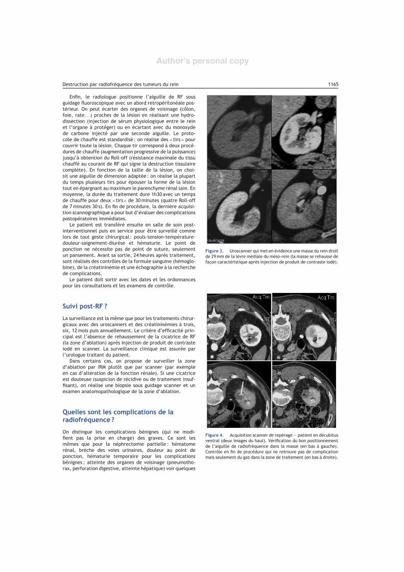
Author's personal copy
Destruction par radiofréquence des tumeurs du rein 1165
Enfin, le radiologue positionne l’aiguille de RF sousguidage fluoroscopique avec un abord retropéritonéale pos-térieur. On peut écarter des organes de voisinage (côlon,foie, rate. . .) proches de la lésion en réalisant une hydro-dissection (injection de sérum physiologique entre le reinet l’organe à protéger) ou en écartant avec du monoxydede carbone injecté par une seconde aiguille. Le proto-cole de chauffe est standardisé : on réalise des « tirs » pourcouvrir toute la lésion. Chaque tir correspond à deux procé-dures de chauffe (augmentation progressive de la puissance)jusqu’à obtention du Roll-off (résistance maximale du tissuchauffé au courant de RF qui signe la destruction tissulairecomplète). En fonction de la taille de la lésion, on choi-sit une aiguille de dimension adaptée : on réalise la plupartdu temps plusieurs tirs pour épouser la forme de la lésiontout en épargnant au maximum le parenchyme rénal sain. Enmoyenne, la durée du traitement dure 1h30 avec un tempsde chauffe pour deux « tirs » de 30 minutes (quatre Roll-offde 7 minutes 30 s). En fin de procédure, la dernière acquisi-tion scannographique a pour but d’évaluer des complicationspostopératoires immédiates.
Le patient est transféré ensuite en salle de soin post-interventionnel puis en service pour être surveillé commelors de tout geste chirurgical : pouls-tension-température-douleur-saignement-diurèse et hématurie. Le point deponction ne nécessite pas de point de suture, seulementun pansement. Avant sa sortie, 24 heures après traitement,sont réalisés des contrôles de la formule sanguine (hémoglo-bine), de la créatininémie et une échographie à la recherchede complications.
Le patient doit sortir avec les dates et les ordonnancespour les consultations et les examens de contrôle.
Suivi post-RF ?
La surveillance est la même que pour les traitements chirur-gicaux avec des uroscanners et des créatininémies à trois,six, 12 mois puis annuellement. Le critère d’efficacité prin-cipal est l’absence de rehaussement de la cicatrice de RF(la zone d’ablation) après injection de produit de contrasteiodé en scanner. La surveillance clinique est assurée parl’urologue traitant du patient.
Dans certains cas, on propose de surveiller la zoned’ablation par IRM plutôt que par scanner (par exempleen cas d’altération de la fonction rénale). Si une cicatriceest douteuse (suspicion de récidive ou de traitement insuf-fisant), on réalise une biopsie sous guidage scanner et unexamen anatomopathologique de la zone d’ablation.
Quelles sont les complications de laradiofréquence ?
On distingue les complications bénignes (qui ne modi-fient pas la prise en charge) des graves. Ce sont lesmêmes que pour la néphrectomie partielle : hématomerénal, brèche des voies urinaires, douleur au point deponction, hématurie temporaire pour les complicationsbénignes ; atteinte des organes de voisinage (pneumotho-rax, perforation digestive, atteinte hépatique) voir quelques
Figure 3. Uroscanner qui met en évidence une masse du rein droitde 29 mm de la lèvre médiale du méso-rein (la masse se rehausse defacon caractéristique après injection de produit de contraste iodé).
Figure 4. Acquisition scanner de repérage — patient en décubitusventral (deux images du haut). Vérification du bon positionnementde l’aiguille de radiofréquence dans la masse (en bas à gauche).Contrôle en fin de procédure qui ne retrouve pas de complicationmais seulement du gaz dans la zone de traitement (en bas à droite).

Author's personal copy
1166 P. Souteyrand et al.
Figure 5. Échographie de contrôle à 24 h : pas de complication locale, le rein est vascularisé en doppler.
exceptionnelles complications létales (embolie pulmonairesmassives. . .).
Intérêts de la radiofréquence rénale etcomparaison par rapport à la chirurgiepartielle
Son efficacité oncologique est de 90 à 95 % [4], ce qui estéquivalent à la chirurgie partielle. Par contre son effica-cité fonctionnelle est supérieure puisque la diminution dudébit de filtration glomérulaire (le reflet de son fonctionne-ment) est de moins de 2 % contre 30 % pour les néphrectomiespartielles. Cette variation ne dépend pas de la taille de latumeur contrairement aux néphrectomies partielles [5]. Letaux de complications bénignes et graves est similaire pourles deux techniques 3,1 et 1,25 %. La durée d’hospitalisationest par ailleurs raccourcie (deux jours au lieu de cinq enmoyenne).
Figure 6. Échographie de contrôle à 18 mois.
Un exemple
Une masse du rein droit de 29 mm est découverte de faconfortuite sur un scanner (Fig. 3) chez un homme de 81 anssans antécédent. Il a bénéficié d’une biopsie rénale scan-noguidée qui a confirmée le diagnostic de carcinome àcellules conventionnelles de grade II de Führman. Le traite-ment curatif par RF a été validé en Réunion de concertationpluridisciplinaire. En consultation pré-RF, son consentementa été recueilli. Le patient a été traité sous anesthé-sie générale et avec un guidage fluoroscopique (Fig. 4)selon les protocoles de chauffe habituels. Il a été hospita-lisé 24 heures en urologie avec un contrôle échographiqueavant la sortie (Fig. 5) pour éliminer des complications.La surveillance s’est déroulé normalement avec, sur lescanner à 18 mois (Fig. 6), une cicatrice de 20 mm quine se rehaussait pas, ce qui attestait d’un traitementefficace.
En conclusion
La RF est une alternative thérapeutique fiable qui complètel’arsenal thérapeutique proposé à l’urologue puisque lesrésultats carcinologiques sont validés. C’est un traitementpour des patients non opérables (indication de nécessité)mais aussi une solution qui peut être choisie par le patient(indication élective).
Cette technique moderne et fiable ne bénéfice d’aucunfinancement, ce qui la réserve pour l’instant à des centresréférents. Sa reconnaissance par les autorités de tutelledevrait permettre de la diffuser plus largement.
Déclaration d’intérêts
Les auteurs déclarent ne pas avoir de conflits d’intérêts enrelation avec cet article.
Références
[1] Méjean A, André M, Doublet JD, Fendler JP, de Fromont M, Hélé-non O, et al. Kidney tumors. Prog Urol 2004;14(4 Suppl. 1):997[999—1035].

Author's personal copy
Destruction par radiofréquence des tumeurs du rein 1167
[2] Mejean A, Correas JM, Escudier B, de Fromont M, Lang H, LongJA, et al. Kidney tumors. Prog Urol 2007;17(6):1101—44.
[3] Zagoria RJ, Pettus JA, Rogers M, Werle DM,Childs D, Leyendecker JR. Long-term outcomesafter percutaneous radiofrequency ablation forrenal cell carcinoma. Urology 2011;77(6):1393—7,http://dx.doi.org/10.1016/j.urology.2010.12.077 [Epub2011 Apr 13].
[4] Gervais DA, Arellano RS, Mueller PR. Percutaneous radio-frequency ablation of renal cell carcinoma. Eur Radiol2005;15(5):960—7 [Epub 2005 Mar 9].
[5] Pettus JA, Werle DM, Saunders W, Hemal A, Kader AK, ChildsD, et al. Percutaneous radiofrequency ablation does not affectglomerular filtration rate. J Endourol 2010;24(10):1687—91,http://dx.doi.org/10.1089/end.2010.0029.

Disponible en ligne sur
www.sciencedirect.com
ARTICLE ORIGINAL
Cicatrice de radiofréquence rénale : corrélationsanatomopathologiques-tomodensitométriques chezle porc. Applications pratiques pour le suivi enimagerie!
Pathological features of radiofrequency ablation (RFA) renal scar CT-imaging ina swine model
P. Souteyrand a,∗, F. Cohenb, L. Danielb,É. Lechevallier c, C. Chagnaud a, P.H. Rollandd,M. Andre a, V. Vidald
a Servide de radiologie, hôpital Conception, AP—HM, 147, boulevard Baille, 13385 Marseille
cedex 05, Franceb Service de radiologie, hôpital Timone, AP—HM, 13005 Marseille, Francec Service d’urologie, hôpital Conception, AP—HM, 147, boulevard Baille, 13385 Marseille
cedex 05, Franced Laboratoire de physiopathologie et de thérapie vasculaire (L2PTV), faculté de médecine,
université Aix Marseille, 13005 Marseille, France
Recu le 20 juin 2012 ; accepté le 1er octobre 2012
MOTS CLÉSRadiofréquence ;Scanner ;Anatomopathologie ;Traitement ablatif
RésuméObjectifs. — Étudier la viabilité tissulaire et identifier les mécanismes d’action de la radiofré-quence (RF) à partir d’une confrontation imagerie—anatomopathologie de lésions de RF rénaleun mois après traitement sur un modèle porcin.Matériels et méthodes. — Vingt-quatre lésions de RF ont été réalisées sur six porcs anesthé-siés (traitement aux deux pôles des deux reins) avec des aiguilles LeVeen 2 cm sous guidagetomodensitométrique. Quatre semaines après traitement, les cicatrices étaient contrôlées enscanner, les reins explantés étudiés en anatomopathologie et en immuno-histochimie.Résultats. — Dix-neuf zones d’ablation (ZA) ont été étudiées en anatomopathologie et en TDM(volume, morphologie, rehaussement, cavitation) quatre semaines après RF. Une ZA abcédée
! Niveau de preuve : 3.∗ Auteur correspondant.
Adresse e-mail : [email protected] (P. Souteyrand).
1166-7087/$ — see front matter © 2012 Elsevier Masson SAS. Tous droits réservés.http://dx.doi.org/10.1016/j.purol.2012.10.004

106 P. Souteyrand et al.
était exclue des résultats ; quatre ZA n’ont pu être analysées en raison du décès précoce d’unporc pendant l’anesthésie. L’histologie des ZA décrivait un aspect hétérogène associant deszones de nécrose, d’ischémie et une surexpression de l’apoptose dans 50 % des ZA. Une nécrosedes ZA était constante en histologie alors que leur rehaussement était variable voire significatif(> 10 UH).Conclusion. — Un mois après traitement, l’examen anatomopathologique des ZA a mis enévidence des destructions tissulaires hétérogènes par différents mécanismes sans viabilité tis-sulaire centrale. Si l’examen TDM post-RF à un mois est utile pour dépister des complicationsiatrogènes, il ne peut prédire l’efficacité du traitement car des lésions ischémiques évolutivesdes ZA persistent. Les contrôles initiaux doivent donc être réalisés au moins trois mois après laRF.© 2012 Elsevier Masson SAS. Tous droits réservés.
KEYWORDSRadiofrequency;CT-scans;Pathology;Ablation techniques
SummaryPurpose. — To analyze the changes in vicinal kidney parenchyma after percutaneous RFA.Materials et methods. — Twenty-four CT-guided RFA procedures were performed on six pigsusing 2 cm LeVeen coaxial needles. We studied volume, morphology, cavitation and enhance-ment of the ablation zones (AZ) before and after the procedure on contrast-injected CT-scans.The kidneys were removed four weeks later and studied in the path lab.Results. — All the procedures were successfully completed. Four weeks later, the CT-scans sho-wed AZ that were either clearly circumscribed or with unclear borders, heterogenous areasassociating necrosis and infarct tissue and mesenchyma showing a process of apoptosis aroundthe edges. A treatment considered as incomplete on the CT-scan (presenting as an enhan-cement) was always associated with necrosis on the histology slides, although the necroticareas behaved in various different ways on the CT-scan after injection of contrast medium: anenhancement of more than 10 HU did not mean that no necrotic tissue was present.Conclusion. — RFA causes heterogenous tissue changes, associating necrotic and ischemic zonesand an apoptotic reaction. The mechanisms of these changes and their therapeutic significanceshould be studied. CT-scans performed immediately after RFA procedure and one month laterare not predictive of the efficacy of the treatment because an enhancement of the AZ does notmean that it is not necrotic. The value of a CT-scan performed one month after the procedureis debatable, because the tissue remodeling that occurs in the kidneys is not definitive at thistime-point.© 2012 Elsevier Masson SAS. All rights reserved.
Introduction
La radiofréquence (RF) est une technique d’ablation ther-mique tumorale par excitation moléculaire par un courantde RF, responsable d’une nécrose de coagulation.
Ses résultats [1] et ses taux de complications [2] équiva-lents à la chirurgie partielle ont permis de définir sa placedans le traitement des tumeurs rénales [3]. L’efficacité dutraitement est évaluée en imagerie par l’absence de rehaus-sement significatif après injection de produit de contraste[4], sans qu’il n’y ait jamais eu de confrontation entrel’imagerie et les lésions histologiques pour valider ce cri-tère.
De nombreuses équipes pratiquent un premier contrôle à24—48 heures ou à mois [5] alors qu’il n’existe pas de consen-sus pour le délai de ces contrôles [6]. Les résultats de cettecorrélation imagerie-histologie de la zone d’ablation (ZA)devaient permettre de préciser l’utilité du contrôle tomo-densitométrique (TDM) précoce en prenant l’histologie enréférence, ainsi que la valeur du rehaussement de la ZA.
Notre étude a eu pour objectif d’analyser la ZA deRF rénale sur un modèle animal, le rein de porc, pourconfronter, pour la première fois, l’aspect TDM de la ZA auxremaniements histologiques induits.
Matériels et méthodes
Le Comité d’éthique pour l’expérimentation animale deMarseille a autorisé cette étude prospective qui s’est dérou-lée sur trois mois.
Protocole de radiofréquence et TDM
Le modèle animal expérimental choisi était le rein sain deporc : il n’existe pas de modèle animal de tumeur rénale,et le rein de porc a une anatomie et une physiologie prochedu rein humain. Le même opérateur a réalisé à chaque pôlede chaque rein de six porcs mâles (race Pietrin, Blossin SA,13-Aubagne, France) (six mois, 40 ± 3 kg) le même protocolede RF que celui pratiqué chez l’Humain pour le traitementdes tumeurs rénales : les porcs sous anesthésie générale,intubés et ventilés, étaient installés en décubitus ventraldans le scanner, les quatre électrodes de retour reliées augénérateur (RF3000® Boston Scientific), une voie veineusepériphérique assurant les apports liquidiens, de médica-ments et du produit de contraste. Le positionnement desaiguilles (Needle LeVeen Superslim® 2 cm Boston Scientific)et le déploiement des baleines dans le cortex rénal étaientcontrôlés en échographie et en TDM.

La cicatrice de RF rénale : aspects anatomopathologiques et tomodensitométriques 107
Les protocoles de chauffe ont suivi les algorithmes propo-sés par le constructeur : paliers de 10 W toutes les minutes àpartir de 20 W jusqu’à obtention d’un premier Roll-off, sui-vie d’une séquence identique jusqu’au deuxième Roll-off (endébutant à la moitié de la puissance du premier Roll-off).
Trois TDM ont été réalisées (en apnée sous anesthésiegénérale) : la première en contraste spontané avant la RF, lesdeux TDM de surveillance immédiatement après la RF (j0) età quatre semaines (j28), sans et après injection (1,5 mL/kgpar injection) au temps néphrographique [7] pour étudierla forme, le volume (obtenu en multipliant les trois plusgrands diamètres par 0,55) et le rehaussement des ZA ets’assurer de l’absence de complication locorégionale. Laphase néphrographique a été privilégiée parce qu’elle cor-respond au délai de référence pour la surveillance des RFrénales [8]. Un rehaussement de moins de 10 UH après injec-tion a été considéré comme un succès en TDM [9,10] ; lanécessité de pratiquer une nouvelle RF en cas de rehausse-ment n’était pas considérée comme un échec mais commeun traitement incomplet [11].
Les porcs ont été sacrifiés quatre semaines après laséance de RF par injection intraveineuse d’un bolus de 15 mgde midazolam et de 25 mg de chlorpromazine avec 20 mLde KCl 15 %. Les reins prélevés étaient fixés dans du formolpendant 48 heures.
Le délai de quatre semaines avait été choisi parce que,dans la littérature [8,12], les lésions histologiques sontconsidérées comme définitives à cette date. Il s’agit du délairecommandé pour le premier contrôle tomodensitométriquede l’efficacité du traitement [5]. Goldberg [13] a défini lazone de parenchyme traité comme la ZA, sans préjuger desa nature histologique.
Examen anatomopathologique
Le même pathologiste spécialiste de la pathologie rénalea examiné les reins prélevés avec une colorationhématoxyline-éosine-safran (HES) et par deux marqueursimmuno-histochimiques, l’anti-CD10 (un marqueur des bor-dures en brosse des tubes contournés proximaux) et laPurified Rabbit Anti-Active Caspase-3 (une anticaspase mar-queur de l’apoptose).
Analyse statistique
Les résultats ont été rapportés en accord avec les Stan-dards for Reporting of Diagnostic Accuracy Criteria (STARD)[14]. Les variables quantitatives ont été exprimées médiane[intervalle interquartile], les variables qualitatives enpourcentage. Après la phase descriptive, une analysecomparative a été conduite à l’aide de tests du Chi2 ou testsexacts de Fisher pour les variables qualitatives, et de testsnon paramétriques (Mann-Whitney, Rho de Spearman) pourles variables quantitatives. Pour tous les tests bilatéraux,une valeur du degré de signification p inférieure à 0,05 a étéconsidérée comme statistiquement significative. Les don-nées statistiques ont été traitées avec le logiciel SPSS V15.
Résultats
Toutes les sessions de RF se sont correctement dérouléesavec obtention des deux Roll-off. Les porcs n’ont pas eu
Figure 1. Scanner de contrôle après la radiofréquence (j0) : lescanner met en évidence comme l’examen macroscopique (Fig. 4)un défaut de rehaussement triangulaire à base périphérique corti-cale qui correspond à un infarctus rénal.
d’altération de l’état général. Un porc est décédé à lafin de la RF des complications de l’anesthésie : ses reinsont été explantés tout de suite après la RF pour êtreexaminés en anatomopathologie. Les autres reins ont étéexplantés quatre semaines après la RF. Les RF des six porcsont donc permis l’étude de 23 ZA : quatre ZA « aiguës » àj0 et 19 « chroniques » à j28 (Tableau 1). Les deux seulescomplications tardives ont été un abcès d’une ZA (excluedes résultats) et une pneumopathie d’inhalation.
TDM post-RF (j0)
La morphologie du défaut de rehaussement des ZA était tri-angulaire à base périphérique corticale dans 84 % (16/19)(Fig. 1) et rondes pour les trois autres ZA. Le rehausse-ment médian des 19 zones étudiées était de 6 UH [3—11]et 26,3 % des ZA se rehaussaient précocement (> 10 UH)de facon homogène et diffuse. Le volume médian des ZAétait de 3,6 cm3 [2,8—4,4]. Des remaniements de cavitation(bulles de densité gazeuse) induits par la RF existaient dans69,4 % des ZA (Fig. 2).
TDM quatre semaines après la radiofréquence
Nous avons retenu dix traitements complets soit 52 % desuccès, huit traitements incomplets (48 %) (Fig. 3) et unabcès de la ZA communiquant avec un abcès du psoas. Lerehaussement médian des ZA était de 9 UH [5—21], leurvolume médian à j28 de 3,2 cm3 [2,6—4,4]. Ces rehausse-ments étaient tous diffus et homogène dans les ZA.
Figure 2. Scanner en fin de procédure avec des remaniements decavitation des deux zones d’ablation.

108 P. Souteyrand et al.
Tableau 1 Tableau des résultats des scanners de contrôle et des examens histologiques.
Scanner Anatomopathologie
Cochon Reht j0 Reht j28 Vol j0 Vol j28 Nécrose Zonemésenchymateuse
Ischémie
827.1 7 50 2,4 2,9 1 0 1827.2 3 80 1,9 1,8 1 0 1827.3 54 39 2,5 1,7 1 0 1827.4 130 59 1,3 2,1 1 0 1828 Mort j0 1 0 1829.1 1 14 2,4 4,3 1 1 1829.2 3 8 3,2 2,9 1 1 1829.3 2 15 1,6 1,8 1 1 1829.4 1 15 5,3 3,1 1 1 1830.1 6 8 2,6 1,7 1 1 1830.2 4 2 1,9 1,7 1 1 1830.3 6 4 2,1 2,1 1 1 1830.4 X X X X 1 1 1831.1 8 Abcès 1,3 Abcès 1 0 1831.2 7 7 3 3,9 1 0 1831.3 16 9 2,5 2,5 1 0 1831.4 5 3 1,6 2,1 1 0 1832.1 0 15 2,9 0,9 1 1 1832.2 12 6 2,7 1,7 1 1 1832.3 4 4 1,9 1,2 1 1 1832.4 11 5 4,2 2,1 1 1 1Moyenne
[déviation std]14 [30,3] 19 HU [22,5] 3,73 [1,46] 3,5 [1,35]
Reht : rehaussement ; Vol : volume ; j0, j28 : jour 0, jour 28 ; X : as de mesure.827.1 : cochon 827, pôle sup. rein droit.827.2 : cochon 827, pôle inf. rein droit.827.3 : cochon 827, pôle sup. rein gauche.827.4 : cochon 827, pôle inf. rein gauche.
L’examen anatomopathologique des zonesd’ablation immédiatement après laradiofréquence
Cet examen a décrit en macroscopie une zone circulaireou triangulaire blanchâtre, correspondant à la ZA (Fig. 4).L’examen histologique des quatre ZA a mis en évidence uneaugmentation de l’éosinophilie cytoplasmique, une perte denetteté des limites cellulaires, un aspect flou des noyaux,une hémorragie interstitielle et sur le trajet de l’aiguille,une infiltration inflammatoire et de la nécrose (dans cer-tains cas un hématome sous-capsulaire ou périrénal). Il yavait aussi une coagulation intravasculaire dans les tissusremaniés. Le marquage de l’apoptose par l’anticaspase étaitpositif, principalement dans la nécrose, mais aussi en péri-phérie de la nécrose.
La répartition de ces lésions était hétérogène au sein desZA. Sur certaines lames, il y avait un enchevêtrement dezones de nécrose, d’infiltrats inflammatoires et de tissussains, alors que sur d’autres lames, les zones étaient trèsbien limitées, comme coupées au couteau (Fig. 5). Dansune ZA, des zones tissulaires mixtes ou au contraire biendifférenciées pouvaient coexister, sans que l’on ait pu sys-tématiser leur répartition.
L’examen anatomopathologique des zonesd’ablation quatre semaines après laradiofréquence
Cet examen a décrit trois zones :• des zones de nécrose (centrale ou périphérique) qui asso-
ciaient perte de l’architecture tissulaire, disparition desnoyaux, pycnose, déformations cellulaires et ruptures desmembranes. Elles correspondaient à de la nécrose de coa-gulation typique (Fig. 6) ;
• des tissus en ischémie ou en souffrance, caractériséspar une coagulation intra-vasculaire, des noyaux irrégu-liers, mais une architecture conservée, dans 100 % desZA ;
• une zone mésenchymateuse inconstante, (50 % des ZAétudiées) correspondant à du tissu fibro-conjonctif, sesituait entre la zone de nécrose et les tissus enischémie.
En immuno-histochimie, la surexpression de l’anti-caspase dans les différentes zones témoignait d’uneapoptose induite par la RF. Cette réaction était constantedans 100 % des ZA, visible en périphérie des ZA et au centreoù elle prédominait.

La cicatrice de RF rénale : aspects anatomopathologiques et tomodensitométriques 109
Discussion
Notre étude avait pour objectif principal d’étudier la via-bilité tissulaire après RF et comme objectif secondaired’identifier les mécanismes d’action de la RF par uneconfrontation histologique et tomodensitométrique (TDM)de lésions de RF rénale un mois après traitement sur unmodèle porcin.
Les objectifs et le matériel de l’étude nous imposaientdes limites de choix du modèle expérimental car ces expé-riences n’étaient pas réalisables sur des tumeurs chezdes humains puisqu’elles auraient imposé deux anesthésies(pour la RF et pour la néphrectomie), sans bénéfice cli-nique pour le patient. Les tirs de RF étaient réalisés sur duparenchyme rénal sain de porc parce qu’il n’existait pas demodèle tumoral rénal animal. Notre modèle nous imposaitdonc deux contraintes majeures : extrapoler les résultatsdu porc vers l’humain mais aussi des tissus sains aux tissustumoraux. La seconde limite expérimentale résidait dans ladurée de l’étude limitée à un mois car notre objectif était
de montrer qu’à cette période les remaniements tissulairesn’étaient pas définitivement constitués et pouvaient évo-luer. Une étude plus longue aurait pu permettre d’analyserles remaniements secondaires à la RF au-delà (à trois, six et12 mois comme les contrôles TDM de surveillance).
En tomodensitométrie, les critères de réussite reconnusreposent sur un rehaussement de la ZA inférieur à 10UHaprès injection de produit de contraste [9,10]. Ce critèrede réussite a été défini par analogie avec les études desuivi des tumeurs hépatiques traitées par RF, bien qu’aucuneétude histologique pour le rein n’a jamais été réaliséepour le prouver [15]. Clark parlait même de critère arbi-traire [10]. La persistance d’une réaction inflammatoire(ou d’un tissu de granulation déjà décrit après RF hépa-tique [16]) 4 semaines après traitement était une hypothèsesans preuve histologique. Sur ces examens d’imagerie, leslimites des remaniements tissulaires des ZA à j0 étaientsoit floues avec des plages transitionnelles de composanteshistologiques mixtes (associant tissus sains, nécrotiques etinflammatoires) soit nettes, comme « coupées au couteau ».
Figure 3. Scanners quatre semaines après la radiofréquence. Exemples de mesures de ROI : absence de rehaussement (48 puis 51 UH < 10)qui signe un traitement efficace (1) et un traitement incomplet où le rehaussement (36 puis 64 UH > 10) est significatif (2).

110 P. Souteyrand et al.
Figure 3. (Suite ).
On pouvait alors penser que l’hétérogénéité des rema-niements tissulaires était due à l’association de deuxmécanismes : une ischémie induisant des limites très nettes(par thrombose vasculaire), et l’effet thermique des ondesde RF responsable de limites plus floues. L’analyse tomo-densitométrique du volume de la zone de traitement parrapport au volume théorique de l’ellipsoïde (le volumeenglobé par les baleines d’une aiguille de LeVeen de 2 cmest approximativement de 3,3 cm3) mettait en évidence unezone d’hypodensité de 3,6 cm3 à j0, et de 3,2 cm3 à j28.L’existence d’un infarctus dépassant la zone de traitementthéorique expliquait le volume supérieur de l’hypodensité àj0 au volume théorique traité. La diminution de volume desZA entre j0 et j28 s’expliquait par la rétraction parenchyma-teuse et la résorption de l’œdème.
Les corrélations anatomoradiologique, ont mis en évi-dence un mois après traitement par RF, des zones d’ischémieet de nécrose qui correspondaient en TDM à des imagesd’infarctus hypodenses, triangulaires, à base périphériquecorticale et aux contours bien limités. Ces zones avaientété mises en évidence par Gill [4] qui décrivait déjà la
dévascularisation de la zone traitée en artériographie sanspreuve histologique de l’infarctus tissulaire. L’élévation dela chaleur locale pouvait induire des zones de nécrose pardestruction cellulaire et des zones d’ischémie par destruc-tion des pédicules artériels afférents.
Sur des contrôles TDM très précoce, alors que Lui [17]suggérait, la possibilité de rehaussement dans du tissunécrotique, notre étude prouvait que dans 26 % des cas ilexistait à j0 des rehaussements significatifs dans la ZA alorsque ces zones contenaient sur l’analyse histologique défini-tive des zones de nécrose non viables.
La persistance des tissus en ischémie dans 100 % desZA à j28 était surprenante car on pouvait s’attendre à uneévolution vers une nécrose ou vers une re-perfusion. La per-sistance de tissus en ischémie à un mois signifiait que lesremaniements post-RF n’étaient pas définitivement consti-tués.
Si l’absence de rehaussement pouvait être considéréecomme un critère de réussite du traitement (puisqu’il étaittoujours corrélé à de la nécrose), le rehaussement de la ZAà un mois ne pouvait être considéré comme un échec : le

La cicatrice de RF rénale : aspects anatomopathologiques et tomodensitométriques 111
Figure 4. Aspect macroscopique de la zone d’ablation immédiatement après la radiofréquence : coupes axiale et sagittale d’un rein :infarctus rénal à base périphérique corticale (flèche blanche) et hématome péri-capsulaire (flèche noire) secondaire à la ponction parl’aiguille de radiofréquence. Il s’agit d’un des reins du porc 828 explanté immédiatement après la procédure de radiofréquence.
Figure 5. Zone d’ablation étudiée en immuno-histochimie avec le marqueur de l’apoptose : les régions colorées en marron sont marquéespar l’anticaspase 3 et témoignent de phénomènes d’apoptose. On distingue sur les deux lames (zoom × 100 et × 200) : 1- tissu rénal sainassocié à une souffrance des tubes (qui correspond à l’ischémie), 2- zone mésenchymateuse, 3- nécrose tissulaire, 4- coagulation intravasculaire, 5- marquage nucléaire de l’apoptose.
Figure 6. Lames des zones d’ablation 4 semaines après la procédure (coloration HES, zoom × 50 et × 100) : 1- nécrose tissulaire, 2- zonemésenchymateuse, 3- tissu rénal sain associé à une souffrance des tubes (qui correspond à l’ischémie).

112 P. Souteyrand et al.
rehaussement de la ZA devait être considéré en associationavec la progression volumétrique [8] et l’hétérogénéité durehaussement.
L’élément le plus étonnant était la découverte dezones d’apoptose de distribution hétérogène puisqu’iln’existait aucune répartition topographique systématisablede l’apoptose : le marquage était d’une facon prévisiblepositif au centre mais aussi en périphérie de la zone detraitement, distinct des zones probables d’élévation de latempérature, dans des tissus sains. L’ischémie et la chaleurinduite n’étaient donc probablement pas les seuls méca-nismes de destruction cellulaire induits par la RF sauf sil’on pouvait considérer une répartition inhomogène de latempérature avec des zones d’échauffement sub-critiquesou d’autres phénomènes de dénaturation protéique parl’application locale d’ondes électromagnétiques à hautesfréquences et hautes énergies.
Conclusion
Cette étude a mis en évidence des remaniements tissulaireshétérogènes dans leur forme et leur distribution : des tissusen ischémie, inflammatoires, mésenchymateux ou nécro-sés aux limites nettes ou flous, et une surexpression del’apoptose. Ces remaniements anatomopathologiques n’ontpas pu tous être corrélés formellement avec leur aspecttomodensitométriques. Ces résultats ont remis en questiondes dogmes sur la RF rénale comme l’intérêt du contrôletomodensitométrique post-RF, le délai du premier contrôlede surveillance et le rehaussement de la ZA comme critèred’insuffisance de traitement.
Elle proposait de différer au-delà d’un mois après la RF lepremier contrôle tomodensitométrique, d’associer systéma-tiquement l’étude du rehaussement de la ZA à la répartitiondu rehaussement et à la progression volumétrique.
La mise en évidence d’une réaction d’apoptose induitepar la RF au sein de tissus sain à distance de la zone detraitement signifiait que la nécrose secondaire à l’élévationde la température locale n’était peut être pas la seule voiede destruction tissulaire et ouvrait de nouvelles voies derecherche.
Déclaration d’intérêts
Les auteurs déclarent ne pas avoir de conflits d’intérêts enrelation avec cet article.
Références
[1] Méjean A, Correas JM, Escudier B, de Fromont M, Lang H, LongJA, et al. Kidney tumors. Prog Urol 2007;17(6):1101—44.
[2] Gervais DA, Arellano RS, Mueller PR. Percutaneous radio-frequency ablation of renal cell carcinoma. Eur Radiol2005;15(5):960—7.
[3] Méjean A, André M, Doublet JD, Fendler JP, de Fromont M,Hélénon O, et al. Kidney tumors. Prog Urol 2004;14(4 Suppl.1):999—1035.
[4] Inderbir Gill IS, Hsu TH, Fox RL, Matamoros A, Miller CD,et al. Laparoscopic and percutaneous radiofrequency abla-tion of the kidney: acute and chronic porcine study. Urology2000;56(2):197—200.
[5] Goldberg SN, Gazelle GS, Compton CC, Mueller PR, TanabeKK. Treatment of intrahepatic malignancy with radiofre-quency ablation: radiologic-pathologic correlation. Cancer2000;88(11):2452—63.
[6] Venkatesan AM, Wood BJ, Gervais DA. Percutaneous ablation inthe kidney. Radiology 2011;261(2):375—91.
[7] Debra A, Gervais, Francis J, McGovern, Ronald S, Arellano W,et al. Renal cell carcinoma: clinical experience and technicalsuccess with radio-frequency ablation of 42 tumors. Radiology2003;226:417—24.
[8] Wile GE, Leyendecker JR, Krehbiel KA, Dyer RB, Zagoria RJ. CTand MR imaging after imaging-guided thermal ablation of renalneoplasms. Radiographics 2007;27(2):325—39.
[9] Bossuyt PM, Reitsma JB, Bruns DE, et al. Towards complete andaccurate reporting of studies of diagnostic accuracy: the STARDInitiative. Radiology 2003;226:24—8.
[10] Zagoria RJ, Traver MA, Werle DM, Perini M, Hayasaka S, ClarkPE. Oncologic efficacy of CT-guided percutaneous radiofre-quency ablation of renal cell carcinomas. AJR Am J Roentgenol2007;189(2):429—36.
[11] Clark TW, Millward SF, Gervais DA, Goldberg SN, Grassi CJ,Kinney TB, et al. Reporting standards for percutaneous ther-mal ablation of renal cell carcinoma. J Vasc Interv Radiol2006;17(10):1563—70.
[12] Gervais DA, McGovern FJ, Arellano RS, McDougal WS, Muel-ler PR. Renal cell carcinoma: clinical experience and technicalsuccess with radiofrequency ablation of 42 tumors. Radiology2003;226(2):417—24.
[13] de Baere T, Kuoch V, Smayra T, Dromain C, Cabrera T,Court B, et al. Radiofrequency ablation of renal cell car-cinoma: preliminary clinical experience. J Urol 2002;167(5):1961—4.
[14] Goldberg SN, Grassi CJ, Cardella JF, Charboneau JW, Dodd3rd GD, Dupuy DE, et al. Image-guided tumor ablation: stan-dardization of terminology and reporting criteria. Radiology2005;235(3):728—39.
[15] Goldberg SN, Solbiati L, Hahn PF, et al. Radio-frequencytumor ablation using a clustered electrode technique: resultsin animals and patients with liver metastases. Radiology1998;209:371—9.
[16] Rowland IJ, Rivens I, Chen L, Lebozer CH, Collins DJ, terHaar GR, et al. MRI study of hepatic tumours following highintensity focused ultrasound surgery. Br J Radiol 1997;70:144—53.
[17] Lui KW, Gervais DA, Arellano RA, Mueller PR. Radiofre-quency ablation of renal cell carcinoma. Clin Radiol 2003;58:905—13.

1
Using morphometric scores
to predict RFA complications in renal tumors under 4cm
Purpose: Morphometric scores (MS) can predict the risk of acute intraoperative and
perioperative complications for partial nephrectomies performed for renal tumors.
Radiofrequency (RFA) is an alternative to surgery for those low-grade renal tumors less than
4cm, yet few studies have assessed the value of MS for this ablative technique.
Are MS predictors for the risk of complications after RFA for kidney tumors ?
Materiels and Methods: We identified those patients who received RFA for kidney tumors in our
institution since 2005. The MS (R.E.N.A.L., PADUA and C-Index) and the modified
morphometric scores (MRFS) took into account tumor position and size adaptation criteria. These
were established retrospectively and acute and late complications were reported according to
Clavien classifications.
The relationships between MS and any complications were analyzed by the chi-squared and
Fischer tests.
Results: 160 patients underwent 180 renal RFA treatments (mean follow-up: 25.5 months [1-
106]). There was a single RFA done for 145 patients and multiple RFAs were done for 15
patients in either simultaneous or several staggered treatments. The MS medians were six [5-10]
for PADUA, six [4-10] for R.E.N.A.L., and 2.95 [0.9-12.8] for the C-index. The MRSF medians
were four [3-7] for modified_PADUA, eight [6-12] for PADUA-RFA, four [2-6] for
modified_R.E.N.A.L. and nine [6-13] for R.E.N.A.L.-RFA.

2
There were 13 complications reported (7.22%): seven minor (Clavien I-II) and six major (Clavien
III-IV-V).
There was no correlation between MS and MRSF and the occurrence of any complications
(PADUA, RENAL and C-index: p = 0.32, 0.27 and 0.89).
Conclusions: The known and validated MS for partial surgery did not permit any predictions for
risk after a renal RFA. In particular, neither the size nor the position was a discriminant for
predicting any risk of complications.
Authors:
Philippe Souteyrand MD¹, 2
, Marc André MD¹, Eric Lechevallier MD3, Roch Giorgi MD PhD
4, 5,
6, Christophe Chagnaud MD¹, Romain Boissier MD
3.
1Department of Radiology, Hôpital La Conception APHM, 147 boulevard Baille, 13005
Marseille, France.
²Aix-Marseille Université, LIIE - Laboratoire d'Imagerie Interventionnelle Expérimentale EA
4264, 13005, Marseille, France ³Service de chirurgie urologique, Hôpital La Conception,
Marseille, France. 4Aix-Marseille Université, UMR_S 912 (SESSTIM), IRD, 13385 Marseille, France.
5INSERM, UMR_S 912 (SESSTIM), 13385 Marseille, France.
6APHM, Hôpital Timone, Service Biostatistique et Technologies de l’Information et de la
Communication, 13005, Marseille, France.

3
Manuscript
Introduction
The role of renal radiofrequency (RFA) is defined [1] with results in terms of efficiency, [2] and
complications [3] and is equivalent to those obtained in partial nephrectomies done for renal
masses of 4cm or less.
Nephrometry scoring systems quantify the complexity of renal tumors and are both reliable and
reproducible predictors of pre and postoperative complications of partial nephrectomies [4, 5, 6]
by using pre-operative computed tomography or magnetic resonance imaging. The R.E.N.A.L.
and PADUA scores are validated systems that characterize renal masses based on size, depth, and
their location in relationship to the collecting system or the renal sinus, and polarity [7, 8, 9].
R.E.N.A.L. nephrometry scoring consists of: Radius (tumor size as maximal diameter),
Exophytic/endophytic properties of the tumor, Nearness of the tumor’s deepest portion to the
collecting system or sinus, Anterior (a)/posterior (p) descriptor and the Location relative to the
polar line.
PADUA scoring (Preoperative Aspects and Dimensions Used for an Anatomical classification)
consists of the tumor’s anterior or posterior face, its longitudinal and rim locations, its
relationship to the sinus and urinary collecting system, its percentage of tumor deepening into the
kidney, and its maximal diameter in centimeters.
The C-index was developed to characterize tumor centrality based on the distance ratio between
the tumor, the kidney center and the tumor radius [10].

4
These scores have already been studied for renal thermal ablation, but for the most part, with no
distinction between the percutaneous or laparoscopic access, or between RFA and cryoablation
(CR). Only Schmitt [11] suggests that the R.E.N.A.L. nephrometry scoring system predicts perio-
and post-operative complications in patients undergoing percutaneous renal ablation. Other
authors [12, 13, 14] show no relationship.
Our main objective was to evaluate if morphometric scores played a role in predicting the risk
of complications with renal RFA. We compared these three scores to the series of patients treated
in our center by scanner guided RFA.
Our secondary objective was to propose an optimization of scores for percutaneous ablative
treatments by adapting the tumor size criteria and taking into account the antero-posterior
position of the tumor, which is reported in PADUA and R.E.N.A.L. scores but does not alter
these scores values.

5
Materials and Methods
Our ethics committee gave consent for the retrospective use of the clinical, laboratory and
imaging data of these patients.
All patients treated in our center by renal RFA between January 1st 2005 and December 31st
2014 have been included in this study. The indications for RFA validated by the Tumor Board
respected the following recommendations: clinical T1a (≤4.0 cm) enhancing renal mass after
percutaneous renal mass core biopsy [1].
The MS were calculated by either a preoperative computed tomography (CT) or an MRI. The
criteria viewed as crucial before performing an RFA was the tumor’s depth and position. Because
we wanted to propose an adaptation of PADUA and R.E.N.A.L scores to percutaneous renal
ablative treatments, we independently analyzed and associated the MS and its variables: 1) tumor
position, 2) tumor depth, and 3) the relationship to the renal sinus or collecting system in order to
compare them to the risks of acute complications. The combination of these three parameters
determined the modified-PADUA and modified-R.E.N.A.L scores.
We also proposed two other modified scores: PADUA-RFA and R.E.N.A.L-RFA where two
variables have been modified:
1) size, as suggested by Gahan [15]: 1 score ≤ 3cm / 3cm <2 score ≤ 4cm / 4cm <score 3;
2) position of the posterior tumor (p) score 1 / anterior (a) score 2.

6
For the R.E.N.A.L. and PADUA systems, the scores were totaled and further categorized into
low- (4-6 for R.E.N.A.L. and 6-7 for PADUA), moderate- (7-9 / 8-9) or high-complexity (10-
12/10-13) groups for risk stratification.
The C-index system was further categorized into low complexity (C-index score≥2.5), and high
complexity scores (C-index score <2.5) according to the study of Samplaski and his colleagues
[16].
All RFA were performed under CT-control using general anesthesia with a bipolar RF generator
(RF3000 ® Boston Scientific) and needles (LeVeen Needle ® Boston Scientific). Acute
complications were identified, and classified according to the Clavien-Dindo system [17].
Patients were followed up with CT or MRI imaging with sequences before and after contrast
injection along with acquisitions and reconstruction in the three plans, at 3, 6, and 12 months and
then annually for 10 years [18].
The commonly accepted criteria for success combine size evolution, enhancement of the ablation
zone (AZ) [19], as well as the emergence of new kidney locations or. In case of doubt for a
recurrence, a CT-controlled biopsy was performed. Treatments were only considered effective if
monitoring is longer than six months; otherwise they were excluded from the results.
The examinations were reviewed by the same radiologist (senior imaging uro-nephrology
specialist) on OsiriX software V6.5.2 with results reported on an Excel spreadsheet. Statistical

7
analysis was performed using the R software (version 3.1.0) with a p value <0.05 regarded as
statistically significant.
The continuous variables were described by their mean, standard deviation, and 1st and 3rd
quartile. The categorical variables were described by their numbers and percentage. The effect of
those factors associated with binary acute complications and their efficacy was tested by the chi-
squared test, or Fisher’s exact probability test, for categorical variables, and by the non-
parametric U test of Mann-Whitney for continuous variables. The effect of factors associated
with acute complications coded in three modalities was tested by the chi-squared test or the
probability of Fisher’s exact test for categorical variables, and by the non-parametric Kruskal
Wallis for continuous variables.

8
Results
The 160 patients treated were included in 180 RFA’s overall: 145 patients underwent RFA for an
injury, 10 patients underwent RFA for several different lesions, and five patients received a 2°
RFA on the AZ for a recurrence or for an incomplete treatment.
Of the 10 patients having an RFA for different lesions (synchronous or metachronous), seven
were treated for two lesions; two for three lesions and one for five lesions.
The characteristics of those treated patients are summarized in table 1: 180 tumors were treated
on 111 men and on 49 women. The mean age was 69 (22-86) and the majority were treated for
clear renal cell carcinomas (117-65%).
There were 13 (7.22%) complications identified (table 1). Seven of these were minor (Clavien I-
II classification): three with pain at the probe site and four with a limited hematoma. There were
six major complications (Clavien III-IV-V classifications): four with ureteral obstructions
(percutaneous nephrostomy or ureteral probe). These included two deaths: one due to a ruptured
abdominal aortic aneurysm the day following the RFA and the second from secondary multiple
organ failure 48 hours after RFA. The risk factor was identified as the maintenance of the anti-
angiogenic treatment during the procedure (the patient had not interrupted the treatment which is
contraindicated during RFA).
The results of the three scores and their correlation with complications are reported in table 2.
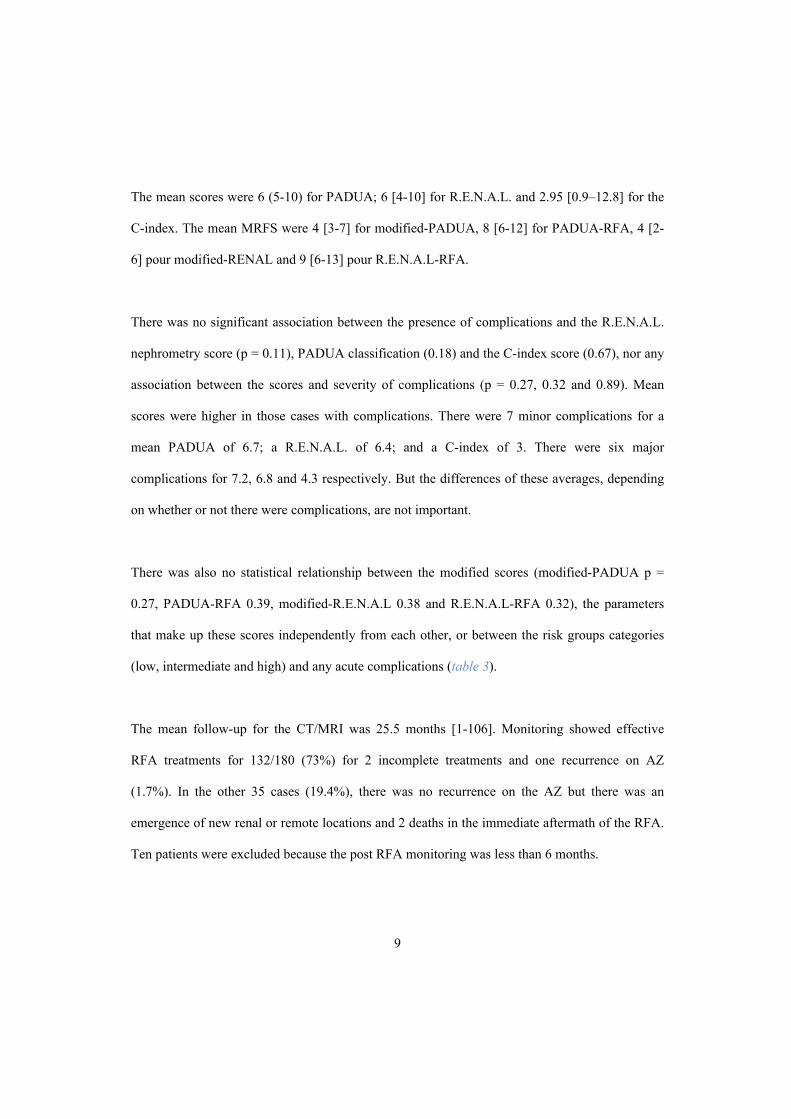
9
The mean scores were 6 (5-10) for PADUA; 6 [4-10] for R.E.N.A.L. and 2.95 [0.9–12.8] for the
C-index. The mean MRFS were 4 [3-7] for modified-PADUA, 8 [6-12] for PADUA-RFA, 4 [2-
6] pour modified-RENAL and 9 [6-13] pour R.E.N.A.L-RFA.
There was no significant association between the presence of complications and the R.E.N.A.L.
nephrometry score (p = 0.11), PADUA classification (0.18) and the C-index score (0.67), nor any
association between the scores and severity of complications (p = 0.27, 0.32 and 0.89). Mean
scores were higher in those cases with complications. There were 7 minor complications for a
mean PADUA of 6.7; a R.E.N.A.L. of 6.4; and a C-index of 3. There were six major
complications for 7.2, 6.8 and 4.3 respectively. But the differences of these averages, depending
on whether or not there were complications, are not important.
There was also no statistical relationship between the modified scores (modified-PADUA p =
0.27, PADUA-RFA 0.39, modified-R.E.N.A.L 0.38 and R.E.N.A.L-RFA 0.32), the parameters
that make up these scores independently from each other, or between the risk groups categories
(low, intermediate and high) and any acute complications (table 3).
The mean follow-up for the CT/MRI was 25.5 months [1-106]. Monitoring showed effective
RFA treatments for 132/180 (73%) for 2 incomplete treatments and one recurrence on AZ
(1.7%). In the other 35 cases (19.4%), there was no recurrence on the AZ but there was an
emergence of new renal or remote locations and 2 deaths in the immediate aftermath of the RFA.
Ten patients were excluded because the post RFA monitoring was less than 6 months.

10
Discussion
Our series was consistent with published RFA series for the distribution of tumor type, size, and
complication rates as well as for long-term results [20].
There were 13 complications identified: 7 minor complications (Clavien I-II) and 6 major
complications (Clavien III-IV-V). There was no significant association between complications
and MS.
Chang [12] also found no association between the scores and complications; however those RFA
were performed laparoscopically. Seidman [13] also found no association between the scores and
complications, but he only analyzed RFA R.E.N.A.L scores without any distinction between a
laparoscopic or a percutaneous approach.
Surprisingly, Schmit [11] suggests that the R.E.N.A.L. nephrometry scoring system predicts
perioperative and postoperative complications in patients undergoing percutaneous R.E.N.A.L.
ablation but without any distinction for RFA and cryoablation (CR).
Okhunov [14] showed that the R.E.N.A.L. score is predictive of cryoablation complications for
small renal masses. There are no publications studying only percutaneous RF scores and
complications.
There are several arguments to explain the lack of any association between the scores and the risk
of acute complications:

11
-the 1st score factor is tumor size with the first level at 4 cm. For RFA, this factor is "1" since it
deals with masses ≤ 4 cm (T1a) and, according to the recommendations of the American
Urological Association (AUA) [1], lesions greater than 4cm are at risk for a sub-optimal
treatment.
Besides, Gahan [15] has already proposed adapting an "m-R.E.N.A.L" modified score where he
adjusts size limit factors (3 and 4 cm rather than 4 and 7 cm) with an improvement in the
performance score.
- According to the AUA [1], an RFA is contraindicated if the sinus or the collector system is
invaded: a 2nd PADUA and R.E.N.A.L factor is stable at 1.
The R.E.N.A.L. and PADUA scores characterized those renal masses that were based, in
particular, on an anterior vs posterior plane. While this factor does not change the score, it is a
fundamental criterion for recommending an RFA. The crucial criteria to consider before
performing an RFA are the tumor depth, position and size. In order to propose PADUA and
R.E.N.A.L score adaptations for renal percutaneous ablative treatments, we independently
analyzed and associated variables: 1) tumor position, 2) tumor depth, and 3) the relationship to
renal sinuses or collective systems, so as to compare the risk of acute complications. The
combination of the three parameters determined both the modified-PADUA and the modified-
R.E.N.A.L scores, which we then compared for risk complications by linking both scores.
To highlight the "location" criterion, which was reported but not recognized for both the PADUA
and R.E.N.A.L. scores, we integrated it with the Gahan score [15] (which modifies the tumor size
criterion) in order to obtain the PADUA-RFA and R.E.N.A.L-RFA scores. Regardless of the

12
independent parameters taken or the modified scores, there is no association to the risk of
complications.
This study has several limitations worth discussing. First, it is limited by the fact that data were
retrospectively analyzed and only one radiologist calculated scores. We considered that these
scores were reproducible and consistent with the literature [9]. Additionally, patients were
selected based on a tumor size not exceeding 4cm, but this size limit was imposed by the RFA
[1].
Conclusion
The PADUA, R.E.N.A.L. and C-index classifications all fail to predict acute complications
associated with RFA treatments. Notably neither tumor size nor position was a discriminant in
predicting the risk of complications. The adaptation of PADUA and R.E.N.A.L. scores along
with criteria modification of size and the integration of the anterior or posterior position of the
tumor do not predict the risk of complications of percutaneous renal RFA. The results of our
study confirmed that RFA is a safe method to treat kidney tumors (clinical T1a ≤4.0 cm). RFA
may be recommended as an elective treatment alternative to surgery and obtains identical
oncological results.

13
References
1. Campbell SC, Novick AC, Belldegrun A, et al. Guideline for management of the clinical
T1 renal mass. J Urol. 2009. 182(4): 1271-9
2. Méjean A, Correas JM, Escudier B, de Fromont M, Lang H, Long JA, Neuzillet Y, Patard
JJ, Piechaud T. [Kidney tumors]. Prog Urol. 2007 Nov;17(6): 1101-1144.
3. D.A. Gervais, R.S. Arellano, P.R. Mueller. Percutaneous Radiofrequency Ablation of
Renal Cell Carcinoma. Eur Radiol. 2005 May;15(5): 960-7.
4. Samplaski MK, Hernandez A, Gill IS, et al. C-index is associated with functional
outcomes after laparoscopic partial nephrectomy. J Urol. 2010. 184(6): 2259-63.
5. Ficarra V, Novara G, Secco S, Macchi V, Porzionato A, De Caro R, Artibani W.
Preoperative aspects and dimensions used for an anatomical (PADUA) classification of
renal tumours in patients who are candidates for nephron-sparing surgery. Eur Urol. 2009
Nov;56(5):786-93. doi: 10.1016/j.eururo.2009.07.040. Epub 2009 Aug 4.
6. Hew MN, Baseskioglu B, Barwari K, et al. Critical appraisal of the PADUA classification
and assessment of the R.E.N.A.L. nephrometry score in patients undergoing partial
nephrectomy. J Urol. 2011. 186(1): 42-6.
7. Kutikov A and Uzzo RG. The R.E.N.A.L. nephrometry score: a comprehensive
standardized system for quantitating renal tumor size, location and depth. J Urol
2009;182:844-53.
8. Matthew N. Simmons, Christina B. Ching, Mary K. Samplaski, Chin Hyong Park,
Inderbir S. Gill. Kidney Tumor Location Measurement Using the C Index Method. The

14
Journal of Urology, Vol.183, May 2010, 1708-1713.
9. Christopher J. Weight, Thomas D. Atwell, Robert T. Fazzio, Simon P. Kim, McCabe
Kenny.A Multidisciplinary Evaluation of Inter-Reviewer Agreement of the Nephrometry
Score and the Prediction of Long-Term Outcomes. J Urol ,Vol. 186, October 2011, 1223-
1228.
10. Simmons MN, Ching CB, Samplaski MK, et al. Kidney tumor location measurement
using the C index method. J Urol. 2010. 183(5): 1708-13.
11. Schmit GD, Thompson RH, Kurup AN et al. Usefulness of R.E.N.A.L. nephrometry
scoring system for predicting outcomes and complications of percutaneous ablation of
751 renal tumors. J Urol 2013; 189: 30–5
12. Chang X, Liu T, Zhang F, Qian C, Ji C, Zhao X, Liu G, Guo H, The comparison of
R.E.N.A.L., PADUA and Centrality Index score in predicting perioperative outcomes and
complications following laparoscopic radiofrequency ablation of renal tumors, The
Journal of Urology (2015), doi: 10.1016/j.juro.2015.03.095.
13. Seideman CA, Gahan J, Weaver M, Olweny EO, Richter M, Chan D, Cadeddu JA. Renal
tumour nephrometry score does not correlate with the risk of radiofrequency ablation
complications. BJU Int. 2013 Dec;112(8):1121-4. doi: 10.1111/bju.12276.
14. Okhunov Z, Shapiro EY, Moreira DM et al. R.E.N.A.L. nephrometry score accurately
predicts complications following laparoscopic renal cryoablation. J Urol 2012; 188:
1796–800
15. Gahan JC, Richter MD, Seideman CA, Trimmer C, Chan D, Weaver M, Olweny EO,
Cadeddu JA. The performance of a modified RENAL nephrometry score in predicting
renal mass radiofrequency ablation success. Urology. 2015 Jan;85(1):125-9. doi:
10.1016/j.urology.2014.08.026. Epub 2014 Oct 18.

15
16. Samplaski MK, Hernandez A, Gill IS, et al. C-index is associated with functional
outcomes after laparoscopic partial nephrectomy. J Urol. 2010. 184(6): 2259-63.
17. Dindo D, Demartines N, Clavien PA. Classification of surgical complications: a new
proposal with evaluation in a cohort of 6336 patients and results of a survey. Ann Surg
2004; 240: 205–13
18. Goldberg SN, Gazelle GS, Compton CC, Mueller PR, Tanabe KK. Treatment of
intrahepatic malignancy with radiofrequency ablation: radiologic-pathologic correlation.
Cancer. 2000 Jun 1;88(11): 2452-2463.
19. Inderbir Gill IS, Hsu TH, Fox RL, Matamoros A, Miller CD, Leveen RF, Grune MT,
Sung GT, Fidler ME. Laparoscopic and percutaneous radiofrequency ablation of the
kidney: acute and chronic porcine study. Urology. 2000 Aug 1;56(2): 197-200.
20. Atwell TD1, Carter RE, Schmit GD, Carr CM, Boorjian SA, Curry TB, Thompson RH,
Kurup AN, Weisbrod AJ, Chow GK, Leibovich BC, Callstrom MR, Patterson DE.
Complications following 573 percutaneous renal radiofrequency and cryoablation
procedures. J Vasc Interv Radiol. 2012 Jan;23(1):48-54. doi: 10.1016/j.jvir.2011.09.008.
Epub 2011 Oct 28.

16
Figure Legends
Table 1: Patient demographics and renal tumor characteristics.
Table 2: The 3 scores and complications.
Table 3: Statistical results:
• Modified-R.E.N.A.L corresponds to R.E.N.A.L. calculated without R or N.
• R.E.N.A.L-RFA corresponds to matches modified-R.E.N.A.L score taking into account
modified size criteria and the position a / p.
• Modified-PADUA corresponds to PADUA score calculated without sinus or size.
• PADUA-RFA corresponds to modified-PADUA score taking into account the modified
size criteria and the position a / p.
• Minor complications (Clavien I-II) and major complications (Clavien III-IV-V).

RFA 180
Number of patients 160
Gender (n,%)
Male 111 (70)
Female 49 (30)
Mean (range) :
Age (years) 69 (22-86)
Tumour size (mm) 23.8 (8-40)
Tumor side (n,%)
Left 79 (48.9)
Right 101 (61.1)
Tumor location (n,%)
Anterior 68 (35.8)
Posterior 112 (62.2)
Exophytic (n,%)
>50% 93 (51.7)
<50% 69 (38.3)
Endophytic 18 (10)
Biopsy data (n,%) 180
Clear renal cell carcinoma 117 (65)
Chromophobe carcinoma 11 (6.2)
Papillary carcinoma 36 (20)
Oncocytoma 8 (4.4)
Angiomyolipoma 2 (1.1)
Other 6 (3.3)
Complications (n, %)
minor (Clavien I-II) 7 (3.9)
I 5 (2.8)
II 2 (1.1)
major (Clavien III-IV-V) 6 (3.3)
III 3 (1.7)
IV 1 (0.5)
V 2 (1.1)
Follow up (month) 25.8
Effective RFA treatments 132 (73.3)
Treatment failures 38 (21.1)
Incomplete treatment or recurrence on ZA 3 (1.7)
New location 35 (19.4)
Excluded (follow-up < 6 months) 10 (5.6)
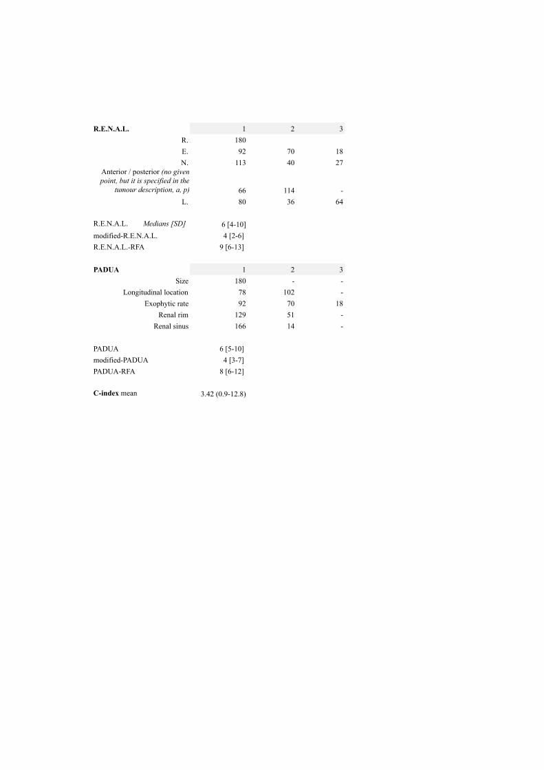
R.E.N.A.L. 1 2 3
R. 180
E. 92 70 18
N. 113 40 27
Anterior / posterior (no given
point, but it is specified in the
tumour description, a, p) 66 114 -
L. 80 36 64
R.E.N.A.L. Medians [SD] 6 [4-10]
modified-R.E.N.A.L. 4 [2-6]
R.E.N.A.L.-RFA 9 [6-13]
PADUA 1 2 3
Size 180 - -
Longitudinal location 78 102 -
Exophytic rate 92 70 18
Renal rim 129 51 -
Renal sinus 166 14 -
PADUA 6 [5-10]
modified-PADUA 4 [3-7]
PADUA-RFA 8 [6-12]
C-index mean 3.42 (0.9-12.8)

Complications
(Clavien)SD 1
st quartile median 3
rd quartileNo patients p
PADUA 0.32
None 1.24 5 6 7 167
I - II (minor) 1.25 6 7 7 7
III - IV - V (major) 0.98 7 7 7 6
PADUA-modified 0.27
None 1.13 3 4 5 167
I - II 1.25 4 5 5 7
III - IV - V 0.63 5 5 5 6
PADUA-RFA 0.39
None 1.42 7 8 9 167
I - II 1.11 7.5 8 9 7
III - IV - V 1.67 8.25 9 9 6
R.E.N.A.L. 0.27
None 1.72 4 6 7 167
I - II 1.81 5.5 6 8 7
III - IV - V 1.47 6 6.5 7.75 6
RENAL-modified 0.38
None 1.27 2 4 5 167
I - II 1.21 3 4 5 7
III - IV - V 0.89 3.25 4 4.75 6
RENAL-RFA 0.32
None 1.87 7 9 10 167
I - II 1.86 7.5 9 11 7
III - IV - V 1.97 8.25 9 10.5 6
C-INDEX 0.89
None 1.62 2.22 3 4.15 167
I - II 1.11 2.41 2.59 3.62 7
III - IV - V 4.23 2.46 2.9 3.41 6
No patients (%)
Complic
ations
(%)
p
PADUA 0.73
Low 6–7 141 (78) 11 (85)
Moderate 8–9 and High ≥10 39 (22) 2 (15)
R.E.N.A.L. 0.24
Low 4–6 111 (62) 7 (54)
Moderate 7–9 and High 10–12 69 (38) 6 (46)

Please cite this article in press as: Desmots F, et al. Morphometric scores for kidney tumours: Use in current practice.Diagnostic and Interventional Imaging (2012), http://dx.doi.org/10.1016/j.diii.2012.07.001
TECHNICAL NOTE / Genito-urinary imaging
Morphometric scores for kidney tumours: Use in
current practice
F. Desmots a, P. Souteyrand a, S. Marciano a,E. Lechevallierb, J.V. Zink a, C. Chagnaud a,M. André a,∗
a Radiology Department, Hôpital La Conception, AP—HM, 147, boulevard Baille,
13385 Marseille cedex 5, Franceb Urology Department, Hôpital La Conception, AP—HM, 147, boulevard Baille, 13385 Marseille
cedex 5, France
KEYWORDSPartial nephrectomy;Morphometric score;Cancer of the kidney;Complications
Tissue masses in the kidney discovered by chance are continuously increasing with thediffusion of imaging in cuts. They make up a very heterogeneous and progressive anato-mopathological contingent, the treatment of which has considerably changed over the past20 years, both in the pretreatment evaluation and in the surgical approach, where par-tial nephrectomy (PN) has become the standard due to its good results on the cancer andprogress in surgical techniques. PNs have been enriched by percutaneous removal treat-ments that complete the therapeutic range offered to patients. However, if PN makeskidney conservation possible with a long-term survival rate that is identical to that oflarger nephrectomise, they cause more common per- and pericomplications (19 to 25%).Currently, if there are not true tumoural prognosis factors, each patient befits in RCPfrom a personalised pre-therapeutic and therapeutic proposal that is locally adapted totechnical settings and medico-surgical teams.
Clinical interest
Like the Bosniak classification, morphometric scores give a ranking based on the size andlocation of the tumour using a CT-scan or MRI.
∗ Corresponding author.E-mail address: [email protected] (M. André).
2211-5684/$ — see front matter © 2012 Éditions francaises de radiologie. Published by Elsevier Masson SAS. All rights reserved.http://dx.doi.org/10.1016/j.diii.2012.07.001

Please cite this article in press as: Desmots F, et al. Morphometric scores for kidney tumours: Use in current practice.Diagnostic and Interventional Imaging (2012), http://dx.doi.org/10.1016/j.diii.2012.07.001
2 F. Desmots et al.
These scores were suggested by Kutikov (RENAL nephrom-etry score) and Ficcara (PADUA) in 2009 and by Simmons(C-Index) in 2010 in order to standardise series and giveradiologists the tools to make it possible to classify tissuemasses and provide information that would allow urologiststo offer suitable therapeutic choices based on objec-tive morphological data [1—3]. The first series publishedusing these classification criteria show a good interobserverreproducibility [4] and provide prognosis evaluation infor-mation on per- and perioperative morbidity [5]. This cansignificantly predict (P < 0.001) the risk of complication,while the size of the lesion or its anterior or poste-rior location taken alone (univariate analysis) does notmake it possible to conclude [1]. In addition, the mor-phometric score is an interesting piece of information forpredicting the peroperative clamping time: the higher thescore (PADUA and R.E.N.A.L.), the longer the ischaemiatime, which indirectly appreciates operative difficulties(P < 0.001) [6].
Anatomical classifications
PADUA
Preoperative Aspects and Dimensions Used for an Anatomicalclassification. This score varies from 6 to 14 (Table 1) andtakes into account five lesional anatomical characteristicsin addition to the maximum diameter. A score of 8 and 9makes it possible to identify patient groups with a risk ofcomplication 14 times higher than with scores of 6 and 7.Concerning the reproducibility of the determination of thePADUA score, the interobserver correlation is approximately73% [5].
RENAL
Radius: maximum diameter of the lesion, E: exophytic orendophytic tumour, N: nearness or tumour extension indepth. This score varies from 4 to 12 (Table 2) to which thetwo suffixes a or p for anterior or posterior are attributedand the letter h if the lesion is in contact with the veinor main artery. In this score, the maximum transverse
Table 2 RENAL morphometric score.
1 point 2 points 3 points
(R)adius (maximum diameter in cm) ≤ 4 > 4 but < 7 ≥ 7
(E)xophytic (exophytic development) ≥ 50% < 50% Entirely endophytic
(N)earness (nearness of the tumour to theurine collection system in mm)
≥ 7 > 4 but < 7 ≤ 4
(A)nterieur/Posterior No given point, but it is specified in the tumour description, a, p or x
(L)ocation (tumour location relative to polarlinesa)
Entirely above theupper polar line orbelow the lowerpolar line
The lesionexceeds thepolar lines
> 50% of the lesion exceeds apolar line or crosses the axialor medio kidney line or islocated entirely between thepolar lines
Suffix ‘‘h’’ assigned to a tumour reachingthe main artery or vein
a A diagram is available on the internet on the website www.nephrometry.com.
Table 1 Preoperative aspects and dimensions used foran anatomical classification morphometric score.
Anatomical descriptionsa Score
Longitudinal tumour location (polar)Superior/inferior 1Mean 2
Exophytic> 50% 1< 50% 2
Endophytic 3
Axial tumour locationLateral 1Medial 2
Sinus of the kidneyNot infiltrated 1Infiltrated 2
Tumour size (cm)≤ 4 14.1—7 2> 7 3
a The anterior or posterior location can be indicated with theletters (‘‘a’’ or ‘‘p’’) after the score.
diameter: R (Radius) is a statistically significant predictivemarker (P = 0.02) of the risk of complication in studies witha single variable. In multivariate studies, a RENAL scoregreater than or equal to 9 is an independent and reliable fac-tor of the risk of complication. A score of 10 to 12 increasesthe risks of major complications 5.4 times [7].
C-Index
Index that calculates the ratio of the distance of the cen-tre of the tumour to the centre of the kidney: c forthe size of the tumour: r C-index = c / r [3]. This score(Fig. 1) varies from 0 with an upper limit dependent onthe size and distance of the tumour from the centre of the

Please cite this article in press as: Desmots F, et al. Morphometric scores for kidney tumours: Use in current practice.Diagnostic and Interventional Imaging (2012), http://dx.doi.org/10.1016/j.diii.2012.07.001
Morphometric scores for kidney tumours: Use in current practice 3
Figure 1. According to Simmons [3], the distance between the two centres of the tumour and the kidney is calculated using the PythagoreanTheorem: c =
√(x2 + y2). The index is obtained by the ratio of the distances of the two centres (C) divided by the ray of the mass.
kidney. A C-index of 2.5 increases, for example, by 30% therisk of a major complication. This method appears to bemore complex to implement and requires a longer learningcurve.
Conclusion
Use of morphometric scores to evaluate kidney tumours isa more rigorous approach to their treatment, even if thesemethods remain imperfect and do not include, for example,the speed of growth and the anatomopathological Fuhrmanscore, which are currently the most commonly used pro-gnostic factors. These classifications are relatively close,and the PADUA score appears to be the easiest to imple-ment. Communication in the CT-scan and MRI reports ofa PADUA or RENAL score should make it possible to makethe prognostic evaluation of kidney tumours by radiologistsmore homogeneous. The use of this score in preoperativeevaluation of percutaneous thermal ablations remains to bedefined.
Disclosure of interest
The authors declare that they have no conflicts of interestconcerning this article.
References
[1] Ficarra V, Novara G, Secco S, Macchi V, Porzionato A, De CaroR, et al. Preoperative aspects and dimensions used for ananatomical (PADUA) classification of renal tumours in patientswho are candidates for nephron-sparing surgery. Eur Urol2009;56:786—93.
[2] Kutikov A, Uzzo RG. The R.E.N.A.L. nephrometry score: a com-prehensive standardized system for quantitating renal tumorsize, location and depth. J Urol 2009;182:844—53.
[3] Simmons MN, Ching CB, Samplaski MK, Park CH, Gill IS. Kidneytumor location measurement using the C-index method. J Urol2010;183(5):1708—13.
[4] Weight CJ, Atwell TD, Fazzio RT, Kim SP, Kenny M, Lohse CM,et al. A multidisciplinary evaluation of inter-reviewer agree-ment of the nephrometry score and the prediction of long-termoutcomes. J Urol 2011;186(4):1223—8.
[5] Hew MN, Baseskioglu B, Barwari K, Axwijk PH, Can C, Horen-blas S, et al. Critical appraisal of the PADUA classificationand assesment of the R.E.N.A.L. nephrometry score in patientsundergoing partial nephrectomy. J Urol 2011;186:42—6.
[6] Simhan J, Smaldone MC, Tsai KJ, Canter DJ, Li T, Kutikov A, et al.Objective measures of renal mass anatomic complexity predictrates of major complications following partial nephrectomy. EurUrol 2011;60(4):724—30.
[7] White MA, Haber GP, Autorino R, Khanna R, Hernandez AV,Forest S, et al. Outcomes of robotic partial nephrectomyfor renal masses with nephrometry score of ≥7. Urology2011;77(4):809—13.

FOR
PEER
REVIE
W O
NLY
A MRI Description of Kidney Motion
Journal: Journal of Magnetic Resonance Imaging
Manuscript ID Draft
Wiley - Manuscript type: Original Research
Classification:
Motion supression algorithms < Imaging technology and safety < Basic Science, Mathematical models of imaging processes < Imaging technology and safety < Basic Science, MRI Guided Therapy < Clinical Science, Lower abdomen (kidneys, retroperitoneum, colon) < Body imaging < Clinical Science
Manuscript Keywords: KIDNEY, MOVEMENT, MRI
Journal of Magnetic Resonance Imaging
Journal of Magnetic Resonance Imaging

FOR
PEER
REVIE
W O
NLY
Title:
A MRI Description of Kidney Motion.
Keywords:
MRI; kidney; movement.
Page 1 of 21
Journal of Magnetic Resonance Imaging
Journal of Magnetic Resonance Imaging
1
2
3
4
5
6
7
8
9
10
11
12
13
14
15
16
17
18
19
20
21
22
23
24
25
26
27
28
29
30
31
32
33
34
35
36
37
38
39
40
41
42
43
44
45
46
47
48
49
50
51
52
53
54
55
56
57
58
59
60

FOR
PEER
REVIE
W O
NLY
Abstract:
Objective.
Ablation therapy of renal mass by focused ultrasound requires a real time estimation of
kidney motion including rotation or deformation. The goal of this project is to analyze kidney
motion with 3D MRI.
Methods.
Ten healthy volunteers were enrolled in this study. They underwent 3D T1 weighted MR
acquisitions at different phases of the respiratory cycle with volume reformation. After
segmentation of kidney contours, kidney motion in the 3 space direction was estimated on
several critical points during different respiratory phases. Kidney rotation and deformation
was also estimated.
Results.
With the MRI semi-automated segmentation algorithm, we determined the positions of three
specific points in the kidney throughout the respiratory cycle and then described the 3D
motion of the kidney. These kidney positional shifts were more important in the cranio-caudal
direction (28.9 ±12.2mm and 23.4 ±14.7 mm for the right and left kidneys); but these were
more complex than a linear excursion since kidney rotation (X 5.9° - Y 1.3° - Z 1° on the
right, and 5.2° - 2° - 3° on the left) was also observed. Its displacement was not linear
between the two extreme positions. We do not observed significant kidney deformation
during the respiratory cycle.
Conclusion.
Our study shows the need for a 4D renal tracking, to be able to target a focal lesion in the
kidney during the respiratory cycle.
Page 2 of 21
Journal of Magnetic Resonance Imaging
Journal of Magnetic Resonance Imaging
1
2
3
4
5
6
7
8
9
10
11
12
13
14
15
16
17
18
19
20
21
22
23
24
25
26
27
28
29
30
31
32
33
34
35
36
37
38
39
40
41
42
43
44
45
46
47
48
49
50
51
52
53
54
55
56
57
58
59
60

FOR
PEER
REVIE
W O
NLY
Introduction
Kidney cancer treatments are shifting towards minimally invasive therapies [1], which prove
to be as effective as open renal surgery, but with lower morbidity, shorter hospitalizations,
reduced costs and unsurpassed patient comfort.
Beside needle radiofrequency ablation or tumorectomy guided by laparoscopy, high intensity
focused ultrasound (HIFU) has been proposed to treat small renal masses in patients with high
surgical risk [2, 3, 4]. Since the kidney is a moving target, it is important to estimate kidney
motion during the respiratory circle in order to implement appropriate motion correction
techniques.
The kidney is a richly vascularized organ that moves during respirations despite its fixations
to both the renal artery and vein and the excretory system. There is lot of variation on its
relative position with adjacent organs (liver, spleen, adrenal glands and intestines) related to
patient morphology. Under ultrasound, renal motion is visible but can only be estimated in 2D
[5]. Thus complex displacement including rotation or kidney deformation cannot be captured.
Transcutaneous ablation of a renal mass requires a very good knowledge of the kidney’s
physiologic motion during the respiration. The goal of this study is to model kidney motion
using 4D MRI acquisition combined with kidney segmentation.
Page 3 of 21
Journal of Magnetic Resonance Imaging
Journal of Magnetic Resonance Imaging
1
2
3
4
5
6
7
8
9
10
11
12
13
14
15
16
17
18
19
20
21
22
23
24
25
26
27
28
29
30
31
32
33
34
35
36
37
38
39
40
41
42
43
44
45
46
47
48
49
50
51
52
53
54
55
56
57
58
59
60

FOR
PEER
REVIE
W O
NLY
Materials and Methods
Ten healthy volunteers were recruited in this study. The only criterion for selecting volunteers
was their ability to maintain a 10 second apnea. This study was approved by our institutional
review board approval and all participants signed a written informed consent.
MR acquisition protocol
This study was conducted on a 3T magnet (Skyra, Siemens Medical, Erlangen, Germany).
T1- weighted 3D flash acquisitions were acquired in the axial plane at 5 different phases of
the respiratory cycle (deep inspiration and expiration, intermediate inspiration/expiration, and
neutral. We used a T1 VIBE sequencing DIXON (TR 4.34 / TE 1.35 (opposed phase), FOV
308*380, Matrix 195*320, Slice thickness 3mm). The acquisition time (including both
kidneys) was less than 10 seconds, which matched the requested apnea time.
The apnea requirements were explained to the volunteers prior to testing to assure maximum
cooperation.
An elastic belt containing a load-sensitive pressure sensor was affixed to the
abdominal-low thoracic wall. A continuous signal was transmitted by the belt depending on
the pressure modeled as a curve to the MRI scan monitor. The monitoring of the respiratory
motion was recorded continuously in order to analyze retrospectively the exact phase of the
respiratory cycle for each breath-hold and 3D acquisitions (Figure 1).
Page 4 of 21
Journal of Magnetic Resonance Imaging
Journal of Magnetic Resonance Imaging
1
2
3
4
5
6
7
8
9
10
11
12
13
14
15
16
17
18
19
20
21
22
23
24
25
26
27
28
29
30
31
32
33
34
35
36
37
38
39
40
41
42
43
44
45
46
47
48
49
50
51
52
53
54
55
56
57
58
59
60

FOR
PEER
REVIE
W O
NLY
Kidney segmentation
The data were processed with a semi-automated segmentation tool based on deformable 3D
models [6, 7 and 8] enabling a robust segmentation of kidney volume. Each kidney was
segmented with inclusion of the renal sinus and its contents. The technician initiated the
segmentation after manual positioning of several points (average 5) to outline the kidney on 2
or 3 axial slices. The software used DICOM data to obtain a volumetric axial, coronal and
sagittal 3D reconstruction of the kidneys (Figure 2). The software generated a mesh volume
via Laplacian optimization by extrapolating the contours (interfaces with signal differences)
to the other planes by iterative deformation [6]. Segmentation was corrected manually in each
plane if needed. The contact areas between the kidneys and liver/spleen or the psoas muscle
are those that generate the most mesh distortion. The volumes obtained were stored using
Visualisation Toolkit (VTK) format.
Analysis of kidney motion
2D displacement assessment
Three points were placed at the kidney barycenter (center of the renal volume), upper and
lower poles. The position of each point was defined by its coordinates x, y and z; the "X-
axis" being the lateral axis in the right-left direction, the "Y-axis" representing the antero-
posterior direction and the "Z-axis" being in the cranio-caudal direction. We measured the
linear distance between the two extreme positions of inspiration and maximum expiration,
then calculated the "curvilinear displacement" distance, which is the 3D distance traveled by a
point throughout the five respiratory stages.
Rotation assessment
To quantify the range of rotation, the principal axes were positioned in the volume
Page 5 of 21
Journal of Magnetic Resonance Imaging
Journal of Magnetic Resonance Imaging
1
2
3
4
5
6
7
8
9
10
11
12
13
14
15
16
17
18
19
20
21
22
23
24
25
26
27
28
29
30
31
32
33
34
35
36
37
38
39
40
41
42
43
44
45
46
47
48
49
50
51
52
53
54
55
56
57
58
59
60

FOR
PEER
REVIE
W O
NLY
reconstructed in maximum inspiration and expiration. Three vectors were traced from the
centroid of the kidney to each of the vertices of the meshes, one along the long axis of the
kidney, one along the short axis of the kidney and the latter perpendicular to the two previous
vectors. With linear algebra, we can isolate the matrix [R] from the equation [E] = [R][I],
where [T] is the rotation matrix between the reference system inserted in the kidney in
maximum expiration [E] and the one in the kidney in maximum inspiration[I].
Deformation analysis
Deformations between the different respiratory stages were computed by comparing deep
expiration and deep inspiration meshes and analyzing their differences [9].
The volumetric overlap error (VOE) is determined using the ratio of intersection and union
between two segmentations, E (deep expiration mesh) and I (deep inspiration mesh). It is
calculated as [10],
E∩I
VOE (E, I) = 1 – × 100%
E∪I
The VOE is 0% for a perfect overlap between segmentations and 100% for segmentations
without any overlap.
All the algorithms were compiled with Matlab software 2013.b (Math-Works, Natick, MA)
on an Intel Core i7-960, 3.20GHz, 12 GB RAM computer.
Data were presented as mean ± standard deviation (SD). A paired Wilcoxon (signed-rank) test
was used to compare means. P values <0.05 were taken to be statistically significant.
Statistical analyses were performed using the SSPS 21 (SPSS Inc., Chicago, IL), version
2.10.0.
Page 6 of 21
Journal of Magnetic Resonance Imaging
Journal of Magnetic Resonance Imaging
1
2
3
4
5
6
7
8
9
10
11
12
13
14
15
16
17
18
19
20
21
22
23
24
25
26
27
28
29
30
31
32
33
34
35
36
37
38
39
40
41
42
43
44
45
46
47
48
49
50
51
52
53
54
55
56
57
58
59
60

FOR
PEER
REVIE
W O
NLY
Results
Five females and five males with an average age of 26.6 [21-34] and an average height of 173
cm [155-189] were enrolled in the study. The average weight of the participants was 66 kg
[40-90] with a BMI of 25 kg/m2
[17-26.2] (Table 2).
Acquisitions in our 10 patients were technically successful with acquisition at 5 different
respiratory phases with a continuous monitoring of respiratory motion. Overall, 20 kidneys
were included in the analysis.
Table 1 summarizes the mean (averaged of 3 directions) maximal linear and curvilinear
displacements for the three points of each kidney. The kidney centroid linear displacements
was statistically higher on the left than the right side and was respectively estimated at 31.3
±11.4 mm on the right, and 25 ±14.1mm on the left (p=0.047). Curvilinear displacements
through the five respiratory phases were estimated at 37.3 ±15.6 mm on the right and
42.4±18.8mm on the left (p>0.05). For all patients the curvilinear displacements were higher
than linear displacement (p=0.005 for all comparisons).
For both kidneys, displacement was higher in the cranio-caudal Z (28.9 ±12.2mm for the right
kidney and 23.4 ±14.7 mm for the left kidneys) than lateral X (3.7±3.3 mm for the right and
5.1 ±3.6mm for the left kidneys) and anteroposterior Y (10.4±3mm for the right and 6 ±4mm
for the left kidneys) directions (p<0.05) (Figure 3a). A trend to higher displacement in the
cranio-caudal directions was observed in the right as compared to the left kidney (p=0.058).
On the average, the rotations were estimated at X 5.9° - Y 1.3° - Z 1° on the right, and 5.2° -
2° - 3° on the left kidney (right kidney SD X 9.8°, Y 5.7 and Z 5.3° (range 31.8, 18.4 and
17.6) / left kidney SD X 9.5°, Y 3.7 and Z 5.5° (range 27.7, 12.7 and 18.7)). Rotation varies
from each subject in function of the x, y and z-axis, and Figure 3b shows that rotation can
vary considerably among subjects. Nonetheless, we can deduct, from subject six, that there is
Page 7 of 21
Journal of Magnetic Resonance Imaging
Journal of Magnetic Resonance Imaging
1
2
3
4
5
6
7
8
9
10
11
12
13
14
15
16
17
18
19
20
21
22
23
24
25
26
27
28
29
30
31
32
33
34
35
36
37
38
39
40
41
42
43
44
45
46
47
48
49
50
51
52
53
54
55
56
57
58
59
60

FOR
PEER
REVIE
W O
NLY
a maximum rotation of 20 degrees and an average of 3.1° rotation. While our sample is rather
small, it appears that taller subjects have bigger rotations than do shorter subjects: in our
series, e.g., volunteers under 1.65m never had such calculated displacement exceeding 40 mm,
while those over 1.85m were always higher than 40mm (for right and left kidneys). Kidney
displacement and rotation along the three axes are illustrated in Figure 3b. The average
inspiration volumes were 107cc and 114cc for right and left kidney, 108 and 116 in
expiration: the volume decrease in expiration was not significant (p=0.093 right, p=0.169
left). There was no significant variation in kidney shapes and volumes during the respiratory
cycle (Figure 4).
Page 8 of 21
Journal of Magnetic Resonance Imaging
Journal of Magnetic Resonance Imaging
1
2
3
4
5
6
7
8
9
10
11
12
13
14
15
16
17
18
19
20
21
22
23
24
25
26
27
28
29
30
31
32
33
34
35
36
37
38
39
40
41
42
43
44
45
46
47
48
49
50
51
52
53
54
55
56
57
58
59
60

FOR
PEER
REVIE
W O
NLY
Discussion
Our study shows the complexity of kidney motion during the respiratory cycle, which
includes not only a cranio-caudal but also and antero-posterior and lateral displacement
combined with a rotation component. The last finding of this study is the absence of
deformation during the respiratory cycle. Thus we can assume the kidney is rigid enough to
avoid the use of elastic registration technique more complex to implement.
Curvilinear displacements were higher than linear displacements. These differences show that
kidney displacement is not a rectilinear displacement between the two extreme positions. The
objective was to have a better comprehension of the kidney motion before implementing
dedicated motion correction algorithm. Thus, we believe if it would be not accurate to
perform correction motion based only on two reference volumes taken in the expiratory and
inspiratory position and a basic respiratory compensation triggered by the diaphragm
excursion. This reinforces the importance of developing a real- time kidney tracking
technique.
Several authors have analyzed kidney motion due to respiration, but to our knowledge nobody
analyzes accurately the different dimensions of this complex motion, with MRI. The MRI has
the advantage to combine morphological analysis in the kidney in the three-space direction
and include volume and functional acquisitions during thermal ablation therapies [11].
Song R. et al. [12] analyzed kidney motion related to breathing in MRI. They reported a lower
kidney excursion (8.9±3.7mm) as compared to 23.4±14.7mm in our study. The amplitude
difference can be explained because theirs acquisitions were done during free breathing
whereas our acquisitions were taken in apnea in deep inspiration and expiration. Finally, in
their study Song et al, evaluate only the displacement on the cranio-caudal direction [12].
Page 9 of 21
Journal of Magnetic Resonance Imaging
Journal of Magnetic Resonance Imaging
1
2
3
4
5
6
7
8
9
10
11
12
13
14
15
16
17
18
19
20
21
22
23
24
25
26
27
28
29
30
31
32
33
34
35
36
37
38
39
40
41
42
43
44
45
46
47
48
49
50
51
52
53
54
55
56
57
58
59
60

FOR
PEER
REVIE
W O
NLY
Although Yamashita studies were specific to the kidney centroid, he demonstrated that renal
motion was independent of age, sex, height, or body weight [13]. The absence of correlation
between renal motion and BMI was also confirmed in the study of Song et al. [12]. Abhilash
[14] observed important variations of kidney motions between subjects. However, in our
study the displacement were quite consistent between subjects as shown in figure 3a.
We observed different magnitudes of kidney motion in the three axis with greater excursion in
the cranio-caudal direction as compared to lateral and antero-posterior. This is confirmed by
the study of Tipirneni et al. [16] who only studied one point with a displacement in the three
planes of space, the most important being in the coronal plane whereas other authors have
reported similar displacement in the order of 20mm m in x, y and z axis [14, 15]. Regarding
the latter studies, Doppler ultrasound was used to evaluate kidney motion and this technique
is less reliable than MRI and do not integrate the 3D excursion of the kidney.
The analysis of kidney motion should include different portion of the kidney since we
observed in our study different magnitude of motion between our 3 points of interest in the
three space directions.
Regarding kidney deformation, previous studies suggest that the kidney is a rigid object [12,
14, 15] even if deformation had never been specifically studied by mesh comparison. There
was no significant kidney deformation during the respiratory cycle. The volume variation
observed during the respiratory cycle were within the range of software precision (4.4±1.3%)
[8].
Since there is no kidney deformation, we can conclude the displacements observed in our
study are related to a more complex movement including a rotational component that was not
previously described.
Page 10 of 21
Journal of Magnetic Resonance Imaging
Journal of Magnetic Resonance Imaging
1
2
3
4
5
6
7
8
9
10
11
12
13
14
15
16
17
18
19
20
21
22
23
24
25
26
27
28
29
30
31
32
33
34
35
36
37
38
39
40
41
42
43
44
45
46
47
48
49
50
51
52
53
54
55
56
57
58
59
60

FOR
PEER
REVIE
W O
NLY
Regarding the comparison of displacement between the right and left kidney, we did not find
any meaningful differences: both kidneys moved independently with different amplitudes and
direction especially in the lateral axis. There was no synchronization between the kidney
motion of the right and left kidney.
As shown in our study kidney motion is not limited to the coronal plane. In order to improve
accuracy, the treatments using a 2D tracking such as extracorporeal lithotripsy must take into
account the different components of this motion. The absence of linearity in kidney
displacement and the presence of significant rotation must be considered. Since imaging-
guided treatments can last several minutes, continuous apnea cannot be achieved. Treatments
such as HIFU can last several hours and require an accurate estimation of kidney and tumor
position (margin of error <5 mm in all three axes). A correction based only on the cranio-
caudal direction or a respiratory gating is therefore not sufficient and specific algorithms to
precisely predict kidney and tumor positioned to be developed. This should include a
preoperative 4D modeling of renal motion and real time correction motion during the
respiratory cycle based on fast muliplanar 2D acquisitions that can be registered in the 4D
model.
There is several limitations in our study. First, a larger sample size would help determine if
rotation is an important factor to incorporate in the tracking method and, since our volunteers
were mostly slim, it would be beneficial to study subjects with higher body weight. Second,
we did not correlate the motion of kidney with the motion of the diaphragm because it was
not included in the volume of acquisition.
Page 11 of 21
Journal of Magnetic Resonance Imaging
Journal of Magnetic Resonance Imaging
1
2
3
4
5
6
7
8
9
10
11
12
13
14
15
16
17
18
19
20
21
22
23
24
25
26
27
28
29
30
31
32
33
34
35
36
37
38
39
40
41
42
43
44
45
46
47
48
49
50
51
52
53
54
55
56
57
58
59
60

FOR
PEER
REVIE
W O
NLY
Conclusion
With the MRI semi-automated segmentation algorithm, we determined the positions of three
specific points in the kidney and their excursion during the respiratory cycle to analyze the 3D
motion of the kidney.
These kidney positional shifts are certainly more important in the cranio-caudal direction;
however the anterior-posterior and medio-lateral planes must not be ignored. These are
certainly more complex than a single isolated movement with a notably kidney rotational
component. Its displacement is not linear between the two extreme positions.
With regards to transcutaneous focal treatments, we cannot simply be content with respiratory
synchronization. Our study shows the need for a 4D renal targeted "tracking", which is now
under development.
Page 12 of 21
Journal of Magnetic Resonance Imaging
Journal of Magnetic Resonance Imaging
1
2
3
4
5
6
7
8
9
10
11
12
13
14
15
16
17
18
19
20
21
22
23
24
25
26
27
28
29
30
31
32
33
34
35
36
37
38
39
40
41
42
43
44
45
46
47
48
49
50
51
52
53
54
55
56
57
58
59
60

FOR
PEER
REVIE
W O
NLY
Bibliographie
[1] Thompson RH, Atwell T, Schmit G, Lohse CM, Kurup AN, Weisbrod A, Psutka SP,
Stewart SB, Callstrom MR, Cheville JC, Boorjian SA, Leibovich BC. Comparison of partial
nephrectomy and percutaneous ablation for cT1 renal masses. Eur Urol. 2015 Feb;67(2):252-
9. doi: 10.1016/j.eururo.2014.07.021. Epub 2014 Aug 6.
[2] Hinshaw JL, Lubner MG, Ziemlewicz TJ, Lee FT Jr, Brace CL. Percutaneous tumor
ablation tools: microwave, radiofrequency, or cryoablation--what should you use and why?
Radiographics. 2014 Sep-Oct;34(5):1344-62. doi: 10.1148/rg.345140054.
[3] Luo J, Ren X, Yu T. Efficacy of extracorporeal ultrasound-guided high intensity focused
ultrasound: An evaluation based on controlled trials in China. Int J Radiat Biol. 2015
Jun;91(6):480-5. doi: 10.3109/09553002.2015.1021962. Epub 2015 Mar 28.
[4] MR-Guided Focused Ultrasound Therapy in Oncology. Med Phys. 2015 Jun;42(6):3598.
doi: 10.1118/1.4925562.
[5] Davies SC, Hill AL, Holmes RB, Halliwell M, Jackson PC. Ultrasound quantitation of
respiratory organ motion in the upper abdomen. Br J Radiol. 1994 Nov;67(803):1096-102.
[6] Chartrand, G. Cresson, T. ; Chav, R. ; Gotra, A. ; Tang, A. ; De Guise, J. SEMI-automated
liver CT segmentation using Laplacian meshes. Biomedical Imaging (ISBI), 2014 IEEE 11th
International Symposium on. April 29 2014-May 2 2014. Beijing, China.
Page 13 of 21
Journal of Magnetic Resonance Imaging
Journal of Magnetic Resonance Imaging
1
2
3
4
5
6
7
8
9
10
11
12
13
14
15
16
17
18
19
20
21
22
23
24
25
26
27
28
29
30
31
32
33
34
35
36
37
38
39
40
41
42
43
44
45
46
47
48
49
50
51
52
53
54
55
56
57
58
59
60

FOR
PEER
REVIE
W O
NLY
[7] Chav, R. Cresson, T. ; Chartrand, G. ; Kauffmann, C. ; Soulez, G. ; de Guise, J. A kidney
segmentation from a single prior shape in MRI. Biomedical Imaging (ISBI), 2014 IEEE 11th
International Symposium on. April 29 2014-May 2 2014. Beijing, China.
[8] Gotra A, Chartrand G, Massicotte-Tisluck K, Morin-Roy F, Vandenbroucke-Menu F, de
Guise JA, Tang A. Validation of a Semiautomated Liver Segmentation Method Using CT for
Accurate Volumetry. Acad Radiol. 2015 Apr 20. pii: S1076-6332(15)00131-2. doi:
10.1016/j.acra.2015.03.010.
[9] Extracting Euler Angles from a Rotation Matrix Mike Day, Insomniac Games /
Introduction aux transformations linéaires Algèbre linéaire I — MATH 1057 F Julien
Dompierre.
[10] Heimann T, van Ginneken B, Styner MA, et al. Comparison and evaluation of methods
for liver segmentation from CT datasets. IEEE Trans Med Imaging 2009; 28(8):1251–1265
[11] Quesson B, Laurent C, Maclair G, de Senneville BD, Mougenot C, Ries M, Carteret T,
Rullier A, Moonen CT. Real-time volumetric MRI thermometry of focused ultrasound
ablation in vivo: a feasibility study in pig liver and kidney. NMR Biomed. 2011
Feb;24(2):145-53. doi: 10.1002/nbm.1563. Epub 2010 Dec 3.
[12] R. Song, A. Tipirneni, P. Johnson, R. B. Loeffler, and C. M. Hillenbrand. Evaluation of
respiratory liver and kidney movement for MRI navigator gating. Journal of Magnetic
Resonance Imaging , vol. 33, pp. 143–148, Jan. 2011.
Page 14 of 21
Journal of Magnetic Resonance Imaging
Journal of Magnetic Resonance Imaging
1
2
3
4
5
6
7
8
9
10
11
12
13
14
15
16
17
18
19
20
21
22
23
24
25
26
27
28
29
30
31
32
33
34
35
36
37
38
39
40
41
42
43
44
45
46
47
48
49
50
51
52
53
54
55
56
57
58
59
60

FOR
PEER
REVIE
W O
NLY
[13] Yamashita H, Yamashita M, Futaguchi M, Takenaka R, Shibata S, Yamamoto K,
Nomoto A, Sakumi A, Kida S, Kaneko Y, Takenaka S, Shiraki T, Nakagawa K. Individually
wide range of renal motion evaluated by four-dimensional computed tomography.
Springerplus. 2014 Mar 7;3:131. doi: 10.1186/2193-1801-3-131. eCollection 2014.
[14] R. Abhilash and S. Chauhan. Respiration-induced movement correlation for synchronous
noninvasive renal cancer surgery. IEEE Trans Ultrason Ferroelectr Freq Control. 2012
Jul;59(7):1478-86.
[15] Rakkunedeth H. Abhilash and Sunita Chauhan, Respiration-Induced movement
Correlation for Synchronous Noninvasive Renal Cancer Surgery. IEEE Trans Ultrason
Ferroelectr Freq Control 2012 Jul;59(7):1478-86
[16] A. Tipirneni, R. Song, R. B. Loeffler, C. M. Hillenbrand. Evaluation of the relationship
between respiratory hepatic and renal motion using real-time MRI. Proc. Intl. Soc. Mag.
Reson. Med. 17 (2009).
[17] Peter Rogelj, Frank G. Zöllner, Stanislav Kovačič, Arvid Lundervold."Motion correction
of contrast-enhanced MRI time series of kidney". In: B. Zajc (ed.), Proceedings of the
International Electrotechnical and Computer Science Conference ERK 2007, pp.191-194.
IEEE Region 8, Slovenia section IEEE, September 2007.
Page 15 of 21
Journal of Magnetic Resonance Imaging
Journal of Magnetic Resonance Imaging
1
2
3
4
5
6
7
8
9
10
11
12
13
14
15
16
17
18
19
20
21
22
23
24
25
26
27
28
29
30
31
32
33
34
35
36
37
38
39
40
41
42
43
44
45
46
47
48
49
50
51
52
53
54
55
56
57
58
59
60

FOR
PEER
REVIE
W O
NLY
Figure 1: respiratory cycle schematics. 1a: representation of the physiological respiratory and segmentation cycles. The first curve is a theoretical
curve.
1b: Breathing cycle during apnea. Visualizing a breathing cycle in real-time confirms the actual moment of apnea. Recording the start of the 3D sequence (red line) correlates to the respiratory cycle and enables a
retrospective gating.
125x106mm (96 x 96 DPI)
Page 16 of 21
Journal of Magnetic Resonance Imaging
Journal of Magnetic Resonance Imaging
1
2
3
4
5
6
7
8
9
10
11
12
13
14
15
16
17
18
19
20
21
22
23
24
25
26
27
28
29
30
31
32
33
34
35
36
37
38
39
40
41
42
43
44
45
46
47
48
49
50
51
52
53
54
55
56
57
58
59
60

FOR
PEER
REVIE
W O
NLY
Figure 2: Mesh volume of right kidney enabling the coordinates of the superior, inferior and center poles. The technician initiated the segmentation after manual positioning of several points (red) to outline the
kidney on axial and coronal slices.
73x59mm (72 x 72 DPI)
Page 17 of 21
Journal of Magnetic Resonance Imaging
Journal of Magnetic Resonance Imaging
1
2
3
4
5
6
7
8
9
10
11
12
13
14
15
16
17
18
19
20
21
22
23
24
25
26
27
28
29
30
31
32
33
34
35
36
37
38
39
40
41
42
43
44
45
46
47
48
49
50
51
52
53
54
55
56
57
58
59
60

FOR
PEER
REVIE
W O
NLY
Figure 3: Summary of kidney centroid’s linear displacement and kidney rotations. a) Red points represent the centroid displacement in the x axis, green points in the y axis and blue points in
the z axis. b) Rotation determined by the transformation of reference placed in the maximum inspiration and expiration
sequences separated in x (Rx), y (Ry) and z (Rz). 178x143mm (96 x 96 DPI)
Page 18 of 21
Journal of Magnetic Resonance Imaging
Journal of Magnetic Resonance Imaging
1
2
3
4
5
6
7
8
9
10
11
12
13
14
15
16
17
18
19
20
21
22
23
24
25
26
27
28
29
30
31
32
33
34
35
36
37
38
39
40
41
42
43
44
45
46
47
48
49
50
51
52
53
54
55
56
57
58
59
60

FOR
PEER
REVIE
W O
NLY
Figure 3: Summary of kidney centroid’s linear displacement and kidney rotations. a) Red points represent the centroid displacement in the x axis, green points in the y axis and blue points in
the z axis.
b) Rotation determined by the transformation of reference placed in the maximum inspiration and expiration sequences separated in x (Rx), y (Ry) and z (Rz).
148x111mm (96 x 96 DPI)
Page 19 of 21
Journal of Magnetic Resonance Imaging
Journal of Magnetic Resonance Imaging
1
2
3
4
5
6
7
8
9
10
11
12
13
14
15
16
17
18
19
20
21
22
23
24
25
26
27
28
29
30
31
32
33
34
35
36
37
38
39
40
41
42
43
44
45
46
47
48
49
50
51
52
53
54
55
56
57
58
59
60

FOR
PEER
REVIE
W O
NLY
Figure 4: Right kidney - volunteer 2: anterior-posterior (AP) and posterior-anterior (PA) three-dimensional renderings comparing surface distance error between inspiration and expiration.
Areas in blue represent absence of error (perfect overlap) and areas in yellow represent surface distance
error (in mm). Small amounts of error are observed at the liver interface and along the inferior vena cava. AP, anterior-posterior; PA, posterior-anterior.
318x180mm (96 x 96 DPI)
Page 20 of 21
Journal of Magnetic Resonance Imaging
Journal of Magnetic Resonance Imaging
1
2
3
4
5
6
7
8
9
10
11
12
13
14
15
16
17
18
19
20
21
22
23
24
25
26
27
28
29
30
31
32
33
34
35
36
37
38
39
40
41
42
43
44
45
46
47
48
49
50
51
52
53
54
55
56
57
58
59
60

FOR
PEER
REVIE
W O
NLY
V
o
l
u
n
t
e
e
r
W
e
i
g
h
t
H
e
i
g
h
t
X
(lateral
)
Displa
cement
(mm)
Y
(antero
posteri
or)
Z
(cranio-
caudal
)
kg cm
Right
centroi
d
kidney
Left Right Left Right Left
1 40 153 0.3 8.2 10.1 6.9 25.8 24.2
2 72 180 1.6 1.2 7.9 3.7 21.2 15.4
3 90 185 1.9 4.1 13.8 11.9 30.6 29.8
4 82 186 4.6 4 14.4 8.2 23.2 29.4
5 70 170 7.1 2.8 12.9 10.7 25.1 24.6
6 79 185 7.4 12.4 6.6 8.3 54.5 54.2
7 45 155 1 3.6 6.4 0.8 14.4 4.5
8 56 171 1.9 6.4 11.1 6.6 33 33
9 77 189 9.7 7.8 12.7 1.8 43.3 8.2
10 49 162 1.5 0.4 8 0.7 17.9 10.4
Mean 66 �73 3.7 5.1 10.4 6.0 28.9 23.4
± SD 3.1 3.6 3.0 4.0 12.2 14.7
V
o
l
u
n
t
e
e
r
Straigh
t
displac
ement
(S)
(mm)
Curvili
gne (C)S C S C S C S C S C
TopRight
kidney
Centro
id
Botto
mTop
Left
kidney
Centro
id
Botto
m
1 24 34.9 27.7 28.0 26.5 32.7 21.9 26.2 26.4 27.5 22.2 26.4
2 20.7 24.2 22.7 23 21.6 29.1 13.5 21.9 15.9 17.4 19.3 20
3 32 42.8 33.6 37.5 36.4 41.7 37.2 47 32.3 40.2 37.5 51.7
4 29.7 61.9 27.7 47.4 30.3 64.3 36.7 56.7 30.8 51.5 31.3 57
5 24.5 29.5 29.1 33.6 28.5 38.7 29.6 38.8 26.9 28.9 35.9 39
6 58.9 74.5 55.4 71 54.9 64.2 64 73.1 56.2 57.8 52.6 61.7
7 16.6 17.5 15.7 18.5 18.8 31.3 5.2 20 5.8 19.2 4.4 22.2
8 30.8 52.9 34.9 39.8 32.1 51.1 28.8 59.9 34.2 65.8 35.9 58.5
9 49.4 57.8 46.2 53.5 46.4 59.4 13.8 82.9 11.5 75.4 13.8 72.7
10 22.9 29.7 19.7 21.2 18.8 22 11 40 10.4 40 13 43
Mean 31.0 42.6 31.3 37.3 31.4 43.5 26.2 46.7 25.0 42.4 26.6 45.2
± SD 13.3 17.6 11.4 15.6 11.2 14.6 16.4 20.3 14.1 18.8 13.8 17.2
Page 21 of 21
Journal of Magnetic Resonance Imaging
Journal of Magnetic Resonance Imaging
1
2
3
4
5
6
7
8
9
10
11
12
13
14
15
16
17
18
19
20
21
22
23
24
25
26
27
28
29
30
31
32
33
34
35
36
37
38
39
40
41
42
43
44
45
46
47
48
49
50
51
52
53
54
55
56
57
58
59
60

103
Conférencesenrapportaveclathèse
A. Leonardi V,Mari JL, Vidal V, DanielM. « 3D Reconstruction from CT-Scan Volume
Dataset–ApplicationtoKidneyModeling».DansSCCG2011,27thSpringconference
on ComputerGraphics, ACMPress Publisher, pp. 141-148. Viničné, Slovaquie, avril
2011.
B. LeonardiV,MariJL,VidalV,DanielM.«Reconstruction3DduVolumeRénalàpartir
d’Acquisitions Scanner Volumiques ». Dans Journées du Groupe de Travail en
ModélisationGéométrique,GTMG2011,pp.83-92.Grenoble,France,mars2011.
C. LeonardiV,Mari JL,VidalV,DanielM.«AMorphingApproachforKidneyDynamic
Modeling-From3DReconstructiontoMotionSimulation».Dans20thInternational
Conference in Central Europe on Computer Graphics, Visualization and Computer
Vision,WSCG2012,pp.179-187.Plzen,RépubliqueTchèque,juin2012.
D. LeonardiV,MariJL,SouteyrandP,FrandonJ,VidalV,DanielM.«RecalageContraint
parCartesdeCourburesDiscrètespourlaModélisationDynamiqueduRein».Dans
JournéesduGroupedeTravailenModélisationGéométrique,GTMG2013,pp.149-
158.Marseille,France,mars2013.
E. LeonardiV,DanielM,VidalV,MariJL.«Opérateursdemorphologiemathématiqueet
exploitationdescourburesdiscrètespour ladétectionde tumeursdansunmodèle
rénal ».Dans JournéesduGroupedeTravail enModélisationGéométrique,GTMG
2014,pp.28-33.Lyon,France,mars2014.
F. Leonardi V, Daniel M, Olofsson N, Souteyrand P, Vidal V, Mari JL. « Kidney 3D
DynamicModelingandTumorTrackingforTherapeuticTranscutaneousTreatment».
DansSurgetica2014.Chambéry,France,décembre2014.
Abréviations
AMU:Aix-MarseilleUniversité
CR:cryoablation
IRM:imagerieparrésonnancemagnétique
LIIE:Laboratoired’ImagerieMédicaleetInterventionnelle
RCP:RéuniondeConcertationPluridisciplinaire
RFA:ablationparradiofréquence
SM:scoresmorphométriques
TDM:scanner
ZA:zoned’ablation

104
Annexe1:classificationOMS2004destumeursrénales
Carcinomerénalfamilial
Tumeursàcellulesrénales
• BénignesAdénomepapillaireOncocytome
• MalignesCarcinomeàcellulesclairesCarcinomekystiquemultiloculaireàcellulesclairesCarcinomepapillairedureinCarcinomechromophobedureinCarcinomedestubescollecteursdeBelliniCarcinomemédullairedureinCarcinomeavectranslocationXp11CarcinomeassociéauneuroblastomeCarcinomefusiformetubuleuxetmucineuxCarcinomeinclassé
Tumeursmétanéphriques
AdénomemétanéphriqueAdénofibromemétanéphriqueTumeurstromalemétanéphrique
Tumeursmixtesépithélialesetmésenchymateuses
NéphromekystiqueTumeurmixteépithélialeetstromaleSarcomesynovial
Tumeursnéphroblastiques
RestesnéphrogéniquesNéphroblastomeNéphroblastomecystiquepartiellementdifférencié
Tumeursneuro-endocrines
TumeurcarcinoïdeCarcinomeneuroendocrineTumeurprimitiveneuroectodermiqueNeuroblastomePhéochromocytome
Autrestumeurs
TumeursmésenchymateusesTumeurshématopoïétiquesetlymphoïdesTumeursgerminalesTumeursmétastatiques

105
Annexe2:critèresdéfinissantlegradenucléairedeFuhrman
[H.Letourneux,V.Lindner,H.Lang,T.Massfelder,N.Meyer,C.Saussine,D.Jacqmin.Reproductibilitédugrade
nucléairedeFuhrman:Avantagesd’unregroupementendeuxgrades.ProgUrol2006;16:281-285]
Grades Taille du noyau Contour du Noyau
Nucléoles Cellules monstrueuses
Grade 1 10mm Régulier 0 ou
imperceptibles
0
Grade 2 15mm Discrètes
irrégularités
Visibles au
grossissement
X400
0
Grade 3 20mm Irrégularités
nettes
Visibles en
X100
0
Grade 4 20mm Irrégularités
nettes
Visibles en
X100
Cellules
monstrueuses
multilobées

106
Annexe3:traductiondelaclassificationTNM2009descarcinomesrénaux
(UICC)
T–TUMEURPRIMITIVE
• TX–Renseignementsinsuffisantspourclasserlatumeurprimitive
• T0–Pasdesignedetumeurprimitive
• T1–Tumeurintrarénale≤7cmdanssonplusgranddiamètre
T1a–tumeur≤4cm
T1b–tumeur>4cmet≤7cm
• T2–Tumeurintrarénale>7cmdanssonplusgranddiamètre,limitéeaurein
T2a–tumeur>7cmet<10cm
T2b–tumeur>10cm,limitéeaurein
• T3 – Tumeur étendue aux veines majeures ou aux tissus périrénaux mais sansenvahissement de la glande surrénale ipsilatérale ni dépassement du fascia deGérota
T3a – Tumeur macroscopiquement étendue à la veine rénale ou à sesbranches segmentaires (contenant des muscles) ou tumeur envahissant lagraissepérirénaleet/ouletissuadipeuxdusinusrénal(hilerénal)maissansdépassementdufasciadeGérota
T3b – Tumeur macroscopiquement étendue à la veine cave au-dessous dudiaphragme
T3c – Tumeur macroscopiquement étendue à la veine cave au-dessus dudiaphragmeouenvahissantlaparoidelaveinecave
• T4 – Tumeur étendue au-delà du fascia de Gérota (y compris l’extension parcontiguïtéàlaglandesurrénaleipsilatérale)
N–ADÉNOPATHIESRÉGIONALES
• NX–Renseignementsinsuffisantspourclasserl’atteintedesganglionslymphatiques
• N0–Pasd’atteintedesganglionslymphatiquesrégionaux
• N1–Atteinted’unseulganglionlymphatiquerégional
• N2–Atteintedeplusd’unganglionlymphatiquerégional
M–MÉTASTASESÀDISTANCE
• M0–Pasdemétastasesàdistance
• M1–Métastasesàdistance

107
Annexe4:notionstechniquesenradiofréquence(ablationthermiquepar
excitationmoléculaireparuncourantdeRF)
• Lecourantderadiofréquenceestuncourantsinusoïdalde400à500KHz.Lesrégions
traverséesparcecourantsubissentuneagitationionique,quiinduitparfrictionentre
lesparticulesunéchauffementtissulaire.Lebutestd'exposerlescellulestumoralesà
une température supérieure à 60° C qui provoque de façon quasi immédiate une
dénaturation cellulaire irréversible. Par contre, il n'est pas souhaitable d'atteindre
une température supérieure à 100° C qui, en provoquant une ébullition et une
carbonisationdestissus,augmenteleurrésistanceélectriqueetaltèrelespossibilités
dediffusiondu courant de radiofréquence, diminuant ainsi la taille de la lésionRF
induite.
• Les différents systèmes adaptent le temps de traitement et l'intensité de courant
délivré, soit en monitorant la température, soit en monitorant les variations de
résistancetissulaireentrel'électrodeetlesplaquesdedispersion(parexempleavec
leRF3000deBostonScientific).
• Laprocéduresedéroulesousanesthésiegénérale,lepatientendécubitusventralsur
la table de scanner (certaines équipes ne choisissent pas comme nous la voie
percutanéemaisplutôtlavoielaparoscopiqueoulalaparotomie).
• Toute la procédure est réalisée sous repérage de l’imagerie: on débute par un
uroscannerquipermetun repérage (masse, vaisseaux, voiesexcrétrices, structures
devoisinage),puisl’aiguilledeRFestpositionnée(extrémitéaucentredelatumeur)
etlesbaleinessontdéployéessouscontrôlefluoroscopique.
• Lechoixdelatailledel’aiguilledépenddelatailledelatumeur(diamètredel’aiguille
égalàceluidelatumeur,voirsupérieurde5mmpourcoaguler5mmdeparenchyme
sainquicorrespondaux«margesdesécurité»).
• Le repérage échographique utilisé par certaines équipes, et pour d’autres organes
(foie), nous semble moins adapté pour le rein: les phénomènes de cavitation
(dégagementdegaz)artefactentlerepérage.
• Dans certaines situations, on peut prévenir l’atteinte d’organe de voisinage en les
écartantdelazonetraitée(parinjectiondesérumphysiologique).
• L’intensité et la durée des paliers de RF suivent les recommandations du
constructeur.
Lapuissancedebaseestde20W,qu’onaugmenteparpalierde10Wtouteslesminutes
jusqu’à ce que l’augmentation brutale ne coupe le générateur («Roll-off»). La RF est
reprise30saprèsl’arrêt,à50%delapuissanceappliquéeauroll-offpuisaugmentéeavec
lesmêmespaliersjusqu’àobtenirun2èmeroll-off.

108
Annexe5:protocoledechauffepréconiséparleconstructeurpourune
aiguilledeLeVeende2cm.
Déployer à 2cm l’électrode LEVEEN™.
PROCEDURE FOIE ET REIN
ALGORHYTME pour électrode LEVEEN de 2cm uniquementREF 26-206, REF 26-206, REF 26-226, REF 26-227
Lancer le traitement : Régler la puissance à
30W. Augmenter de 10W par minute jusqu’à
60W maximum
Vérifier deploiement
complet
ROLL OFF ???Arrêter traitement.
Aiguille
complètement déployée ???
avant 5 minutes
Non
Phase 1 terminée : arrêter.Attendre 30 secondes. Redémarrer au même
endroit à 70% de la puissance du ROLL OFF
Continuer le traitement jusqu’au
ROLL OFF
FIN DU TRAITEMENT
Redémarrer à 50% de la puissance du
ROLL OFF
Oui Si pas de ROLL OFF après 5 minutes, augmenter la puissance de 10W par minutes jusqu’à 60W
maximum et attendre le ROLL OFF
Entre 5 et 15 minutes
Si pas de ROLL OFF après 5 minutes,
augmenter la puissance de 10W par
minutes jusqu’à 60W maximum
Non pas de ROLL OFFArrêt automatique après 15 minutes
Redémarrer immédiatement
à 60W

A Nanoengineered Embolic Agent for Precise Radiofrequency Ablation
PIERRE HENRI ROLLAND,1 JOEL L. BERRY,3 GUILLAUME LOUIS,1,2 LIONEL VELLY,1 VINCENT VIDAL,1,2
PAULINE BRIGE,1 VINUTA MAYAKONDA,3 and DAVID L. CARROLL4
1Experimental Interventional Imaging Laboratory, European Center for Medical Imaging Research, School of Medicine,Aix-Marseille University, Marseilles, France; 2Department of Radiology and Medical Imaging, La Timone Hospital, Marseilles,France; 3Department of Biomedical Engineering, University of Alabama at Birmingham, Birmingham, AL 35294, USA; and
4Center for Nanotechnology and Molecular Materials, Department of Physics, Wake Forest University, Winston-Salem,NC 27109, USA
(Received 13 November 2013; accepted 15 January 2014)
Associate Editor Agata A. Exner oversaw the review of this article.
Abstract—The purpose of the work is to investigate whetherthe electromagnetic properties of multi-walled carbon nano-tubes (MWCNT) in the presence of radiofrequency (RF)energy is (1) safe, and (2) improves the precision of thetherapeutic efficiency of the RF-ablation (RFA) procedure.An in vitro phantom was created for evaluating temperaturenear RF treated nanotubes. For the in vivo study, threebaboons and six pigs were submitted for RFA procedure insuperior/inferior kidney poles embolized with a non-adher-ent, lipophilic embolic agent (marsembol) with or withoutMWCNT. Tissue damage in the surrounding kill zone wasassayed through caspase-3 activation. The in vitro resultsshowed marked heat increase only in the region of thenanotubes. In vivo, necrosis/ischemic damage resulted fromRFA therapy alone, RFA plus marsembol only. In marsem-bol + MWCNT condition, dramatic disruption of cellmembranes and sub-cellular organelles was found whereasthe nuclear membranes and basal cell membranes remainedlargely intact. The marsembol vaporized under RFA andtissue fluid filled the space. This caused the MWCNT tocluster within the new aqueous environment. RFA plusmarsembol + MWCNT created a well-defined demarcationbetween healthy and apoptotic cells as evidenced by amarked reduction of caspase-3 expression. By contrast, therewas a much less defined ablation zone in the absence ofMWCNT. In conclusion, the combination of RFA plusmarsembol + MWCNT embolization delineated the killzone in vitro and in vivo. We demonstrate that MWCNTsremain in the ablation region thus minimizing their migrationto the systemic circulation.
Keywords—Radiofrequency, Ablation, Carbon nanotubes,
Embolic agent.
INTRODUCTION
Ablative therapies are required for small-sized can-
cers in order to overcome the deleterious effects of sys-
temic drugs.5,41However, ablative therapies kill healthy
tissue as well as diseased tissue. Radiofrequency abla-
tion (RFA) guided by computerized tomography (CT)
or ultrasound-guided percutaneous radio-frequency
probe ablation (RFA) is important in the primary
management of a multitude of cancers including renal
cell carcinomas (RCC). This treatment provides low
morbidity andminimal clinical impact on postoperative
renal function.1,4,7,8,14 In spite of this clinical success, it is
difficult to confine the to only cancerous tissue volumes.
Further, image-guided measurements are inadequate to
delineate the kill zone because vaporized tissue cannot
be visualizedwith thesemodalities.1,14,23Selective tumor
embolization prior to RFA is a viable means to define
the tumor margin.1,12
It is known that hyperthermic ablation of tissue is
enhanced in the presence of multi-walled carbon nano-
tubes (MWCNT). Previous results from our group
demonstrated complete tumor ablation in mice treated
with the combination of infrared radiation and
MWCNT.5,9,40,41 These nanoparticles combine the un-
ique physical properties of receiving antennas for elec-
tromagnetic energy and of transducers of energy into
marked heat generation adjacent MWCNT. For in-
stance, the average temperature of theMWCNT-loaded
subcutaneous tumor increased to 74 !C compared with
46 !C in control tumors exposed to NIR laser alone.5,9
Nanoparticle-based therapies currently face major
technical and safety challenges. One of the most impor-
tant considerations is the fate of these particles after they
have achieved their therapeutic action.9,15,25,27,36,38
Address correspondence to Joel L. Berry, Department of Bio-
medical Engineering, University of Alabama at Birmingham, Bir-
mingham, AL 35294, USA. Electronic mail: [email protected]
Annals of Biomedical Engineering (" 2014)
DOI: 10.1007/s10439-014-0977-9
" 2014 Biomedical Engineering Society
Author's personal copy

Nanotube length, diameter, impurities, functionaliza-
tion, and method of administration result in different
pathologies.20 In physiological environments, MWCNT
spontaneously form coarse agglomerates diminishing
their ability to transduce electromagnetic energy to heat.
Moreover, dispersion of MWCNT by injection into a
tumor mass requires keeping these nanoparticles from
exiting into healthy tissue.
Our laboratory has developed an embolic agent
(marsembol) that is a colloidal mixture of radiopaque
lipids and hydrophobic proteins designed to achieve effi-
cient dispersion of MWNCTs.42 The present study relies
upon in vitro and in vivo methods to test the hypothesis
that the killing zonemay be precisely delineated by highly
selective tumor embolisation with an embolic agent
doped with MWCNT that capture and focus the radio-
frequency (RF) energy within the embolized tissue while
minimally affecting the surrounding tissues. The in vitro
study revealed a marked increase in temperature in the
presence of RF that was confined to the region of the
nanotubes. This temperature increase required less time
and lower energies than without nanotubes. We further
report a similar result in the in vivo study that these
MWCNTs are not lost to the systemic circulation.
MATERIALS AND METHODS
Preparation of Embolic Agent: Marsembol and
Multi-Walled Carbon Nanotubes (MWNTs)
A gelatin-resorcinol mixture (37.5 g Rousselot 250
bloom PS acid process gelatin, 2.5 g resorcinol and
CaCl2 (1.25 g) in 48.75 mL water, gently stirred 1 h,
40 !C) was mixed with iodized lipiodol (Gerbet, Roissy,
France) (0.5:2, vol:vol). The lipiodol-loaded cross-
linked gelatin was stabilized by glutaraldehyde and
formaldehyde (0.9 and 15.5% in water) (2.5:0.1, vol:vol,
40 !C, 1 h); 100 mM glycine-chlorhydrate (5:1, vol:vol)
were added to neutralize unreacted aldehydes.42
Multi-walled carbon nanotubes (MWNTs) were pro-
ducedbychemical vapordeposition (CVD) ina two-stage
quartz furnace (hydrogen carrier gas). Ferrocine (2.7% in
toluene) was injected into the preheater (5 mL/h) and
furnace temperature ranged from 600 to 900 !C (1 h).
The resultingMWNTwere 50 nm in diameter and cut by
sonication to about 900 nm in length, and assessed for
purity by TEM (Phillips400).5,9,40,41 The aqueous
MWCNT suspension (3 mgMWNT vortexed/sonicated
five times in 0.1 mL water) was mixed with marsembol
(2.5 mL, stopcock-linked 2-syringes).9,15,25,27,36,38
In Vitro Model
Tissue phantoms were created from 8 g/100 mL
Knox gelatin and 4 g/100 mL sugar-free psyllium
hydrophilic mucilloid fiber added to boiling water and
thoroughly mixed until dissolved. Formalin solution
was added to the mixture and thoroughly mixed again,
poured into centrifuge tubes and cooled until firm.
Two cylindrical tissue models were created by
pouring 10 mL of the gelatin mixture into a centrifuge
tube and placed in the refrigerator. A small well was
created at the surface of the gelatin as a reservoir for
the embolic agent. For the first model, the well was
filled with 200 lL of marsembol. For the second
model, the well was filled with 200 lL of marsembol
and a MWCNT suspension. A clinical RF generator
(Radionics, model RFG-3C lesion generator) was used
as the RF energy source to heat the phantoms. RF
measurements were taken at two points equidistant
from the thermocouple. The first temperature probe
was placed within the well containing marsembol, and
the second temperature probe was placed directly into
the gelatin, outside the hollow oval region (Fig. 1). The
temperature of both regions was recorded simulta-
neously. Measurements were taken at four different
RF powers of 0.5, 1, 1.5, and 2 W and at 20-s intervals
for 120 s. The gelatin and marsembol were allowed to
return to room temperature before proceeding to the
next power.
Animal Model
The Provence Ethics Committee for Experimental
Research (#14, Marseilles, France) approved our
experimental protocol. The rationale for using swine
and baboon as experimental models is as follows: the
swine has a thin cortex but low-flow radial arteries
whereas the baboon has high-flow arcuate and radial
arteries but a very thick cortex compared to
humans.13,16,32 These animals served models for low-
flow and high-flow embolization regions that repre-
sent microcirculatory features in a renal carcinoma.
Three female baboon (Papio Anubis, 5–7 years old,
15–17 kg; Station de primatologie CNRS, 13790
Rousset, France) and six pigs (8 months old,
65 ± 3 kg; Blossin SA, 13-Aubagne, France) were
housed for a two-week acclimatizing period. Anes-
thesia was tiletamine 2.5 mg/kg, zolazepam 2.5 mg/kg
and atropine 50 lg (IM), and propofol 0.6 mg/kg/
10 mL (swine) or 2 mg/kg/10 mL (baboon) (IV) and
maintained with gaseous sevoflurane (1.2%) and
sufentanil (2.5 lg/kg/h). Euthanasia was 15 mg
midazolam + 25 mg chlorpromazine in 20 mL KCl
(15%), bolus IV injection.35
Radiological Procedures
Digital subtraction angiographic Stenoscop and
Fluorostar AEC Systems (GE-MS, Minneapolis,
ROLLAND et al.
Author's personal copy

USA) and Helix-CT-Scanner TomoscanM (Philips,
The Netherlands) were used.18,34 Aorto-renal angio-
grams (Hexabrix Guerbet-Inc., 25 mL, 12 mL/s
(swines), 10 mL, 10 mL/s (baboons) were obtained
through a 5F, 65 cm angiographic UFcatheter (Cordis,
Miami, FL, USA) from percutaneous access (Seldin-
ger, right-SFA, 10 cm-long standard 5F-vascular
sheath (Radiofocus Terumo Corporation, Tokyo, Ja-
pan) over 0.035 inch guide-wire (Radiofocus Terumo
Corporation, Tokyo, Japan). After an interlobular
artery (left-or-right kidney) was catheterized, selec-
tively, the embolic agent was delivered via a Rapid
Transit Microcatheter (Cordis, Miami, FL, USA) to
complete zonal embolization (1.7 ± 0.2 mL). Animals
were given CT-scans before/after the procedure with-
out/with injection (1.5 mL/kg, 90 mL 4 mL/s).
RF Treatment in Animals
One pair of return electrodes per lower limb was
connected to the generator (RF3000# Boston Scien-
tific). LeVeen Superslim# needles (2 cm, Boston Sci-
entific Corp.) percutaneously were advanced to the
desired renal cortex sites, and deployed under imaging
control. The RF protocol necessitated 10 W incre-
ments of RF power every minute from 20 W until the
first roll-off and from half the first roll-off wattage
until the second roll-off occurred.
In the swine (N = 6), the RFA treatment procedure
was applied to the inferior pole of the left and right
kidneys (previously embolized or not) as follows:
Control (RFA only) vs. RFA plus marsembol (N = 2),
control vs. RFA plus marsembol + MWCNT (N = 2)
and RFA plus marsembol vs. RFA plus marsem-
bol + MWCNT (N = 2). The same six-sites protocol
was applied to three baboons, but in both the superior
and inferior lobes in each kidney of each animals.
Pathological Examinations: Statistics
A standardized 4-h time was required for early
caspase-3 activation from the initial RFA procedure to
euthanasia. The kidneys were surgically removed and
perfused with buffered 10% formalin, then sectioned
through the center of the embolization zone, and re-
fixed 2 days later.45 Under radiological guidance and
macroscopic examination, serial sections were cut to
obtain 5 mm thick sagittal slices were obtained. These
slices encompassed the embolized zone and the
apparently unscathed adjacent kidney. Secondary sli-
ces 6–7 mm in thickness were cut at the center,
periphery, and outside of the ablation zone at 25, 50,
and 100% distance relative to the ablation zone.18,34,35
Fragments for transmission electron microscopy
(TEM) examination were re-fixed in glutaraldehyde
(2.5%, v/v) in 0.1 M cacodylate (pH 7.4) buffer for 1 h,
FIGURE 1. In vitro phantom study. Results of application of RF to the marsembol + MWCNT reservoir within the gelatin phantomshow a marked increase in temperature within the well. There is a steep gradient of temperature equidistant from the RF probe butoutside the region of the nanotubes.
A Nanoengineered Embolic Agent for Precise RFA
Author's personal copy

post-fixed in OsO4 2.4% prior progressive alcohol
dehydration. Semi-thin (1 lm) and ultra-thin (70 nm)
sections in epoxyresin Epon812 were cut with diamond
knifes (Leica UltracutE) and stained with uranyl ace-
tate (5% in water) and lead citrate (M in NaOH, 1 M).
TEM investigations were carried out on a Jeol JEM
1400 microscope (80 kV) and image recordings with
MegaView3 system (Olympus).
Pathologic and IHC exams were performed on 4 lm
serial thin sections in paraffin (56 !C Histowax,
Goteborg, Sweden) stained with hematoxylin–eosin–
safranin (HES) and Masson’s trichrome. The Histo-
stain# Kit System (streptavidin–alkaline phosphatase,
DAB chromogen) was used to detect active caspase-3
activity (Zymed Laboratories Inc., San Francisco, CA,
USA). Morphometric analysis was performed using an
automatic video analyzer Nikon Elipse H600L.18,34,35
Data treatment and statistical analyses (Kruskal–
Wallis non-parametric anova and Mann–Whitney U
test) were performed by using Systat12 (SPSS Inc.,
Chicago, IL). A non-parametric kernel density esti-
mator was preferred to rule out a functional form
on the distribution function curves. Results were
expressed as mean ± SD.18
RESULTS
In Vitro
Figure 1 shows the change in temperature between
gelatin and marsembol + MWCNTs using an RF
output of 0.5 W through 2 W up to 120 s. The tem-
perature increased with increasing power in all exper-
imental conditions, which can be accounted for by the
difference in RF susceptibilities of gelatin and mar-
sembol + MWCNTs. The difference in temperature
between the two temperature probes is most evident
at 2 W. Outside the region of the marsembol +
MWCNTs, it required six times longer to achieve the
same temperature of 52 !C.
In Vivo
Embolization and RF Treatments
The interventional protocol was successfully com-
pleted in each animal. Renal embolization was
achieved with marsembol, in the presence or absence of
MWCNTs (Fig. 2). Between the three experimental
groups, there was no statistical significance in energy
FIGURE 2. Imaging the RFA procedure. Digital angiograms of the renal artery at the inferior pole of the right kidney before (topleft) and after (top middle) embolization with MWCNT-loaded marsembol and after RF needle insertion (top right) in a porcinesubject. Renal CT-scans of the implanted RF needle (bottom, left and middle; porcine) and after embolization and RFA procedure(bottom left, baboon).
ROLLAND et al.
Author's personal copy

input or roll-off time/wattage (Table 1). However,
there was a marked tendency for the roll-off values to
be lower in the primates as compared to the swines
(p< 0.10). marsembol + MWCNTs tended to reduce
the RFA treatment time and intensity.
Multi-Walled Carbon Nanotubes and RF Treatments
Multi-walled carbon nanotubes (MWNTs) cluster
into dimensions ranging from 0.1 to 3.0 mm. In order
to disperse the clusters, the first-step was sonication
reducing the cluster size to a 20–50 lm network of
overlapping nanotubes. These networks were intro-
duced into the non-adhesive, lipophilic, and amor-
phous marsembol such that individualized MWCNTs
were dispersed and engulfed in the embolic agent
(Fig. 3). No differences were observed in delivering
marsembol with or without MWCNT through identi-
cal micro-catheters.
The transduction RF energy to heat by the presence
of MWCNTs suspended in marsembol was demon-
strated in separate experiments (Fig. 3). The marsem-
bol + MWCNT mixture and marsembol alone (50:50,
v:v) was delivered into a swine kidney and submitted to
a single-step RF therapy protocol. The procedure
caused marsembol + MWCNT to partially decom-
pose (vaporize) under the RF energy but not in mar-
sembol alone underscoring the efficiency of energy
transduction in the presence of MWCNTs.
Tissue Damage in the Ablation Zone: MWCNT Fate
Gross observation of RFA-induced tissue damage
was similar in the kidneys of the swine and the
baboons (Fig. 4; Table 1). However, there was a ten-
dency for an increased volume of the RFA kill zone in
the baboons, which is presumably to be accounted for
by the higher thickness of the baboon renal cortex, as
compared with the porcine renal cortex. Ablation
using RFA induces the usual cellular and subcellular
damage (necrotic shrinking of cellular components and
ischemic separation of epithelial cell layers from the
renal tubules) whether an embolic agent is present or
not.
Histological observation of ablated marsem-
bol + MWCNT revealed that cell damage showed
dramatic disruption and complete disorganization of
cell membranes, and sub-cellular organelles (Fig. 5).
Identical findings in the porcine and baboon kidneys
supported this observation. Specifically in the mar-
sembol + MWCNT zones, the tubule cell contents
were condensed, and the cell membrane was disag-
gregated and dispersed whereas the nuclear cell mem-
branes and basal membranes remained largely intact.
Using TEM observation of RFA-treated baboon
and swine nephron structures, it was revealed that the
marsembol + MWCNT which once resided within the
very distal arterioles was found to have largely
vaporized (Fig. 6). Some marsembol + MWCNT is-
lets remained. These marsembol + MWCNT residues
were characterized by a homogeneous gray color core
(the usual appearance of marsembol under TEM) and
a border of clustered structures having the size and
appearance of the original non-dispersed structure of
MWCNTs (Fig. 6). These marsembol + MWCNT
residues were detected in cases where the external and
nuclear membranes of renal tubules were preserved
only. Clusters of MWCNTs formed once the mar-
sembol embolic agent vaporized under RF treatment.
The marsembol vaporized under RFA and tissue fluid
filled the space. This caused the MWCNT to cluster
within the new aqueous environment. This clustering
behavior is typical of nanotubes changing from a
lipophilic environment to an aqueous environment.
Tissue Damage Outside the Ablation Zone
The extent to which the RFA procedure damaged
the surrounding tissue was investigated through
observation of the activation of apoptotic cell death.
Activation of caspase-3 was used as an early marker
(within 4 h) of apoptosis (Fig. 7). In all experimental
conditions, the expression of caspase-3 decreased dra-
matically in a volume of tissue extending outward to
twice the diameter of the ablation zone. Figure 7 fur-
ther illustrates that the level of RFA-induced apoptosis
varied depending on whether MWCNTs were present.
TABLE 1. Energy input and roll-off time/wattage in RFA procedures.
Baboon Swine
No embolization Roll-off 1: 5.5 ± 1.6 min/50 W Roll-off 1: 3.5 ± 1.4 min/50 W
Roll-off 2: 4.1 ± 1.6 min/40 W Roll-off 2: 2.5 ± 0.9 min/40 W
Marsembol Roll-off 1: 4.5 ± 1.5 min/50 W Roll-off 1: 3.4 ± 1.1 min/50 W
Roll-off 2: 3.9 ± 1.3 min/40 W Roll-off 2: 2.1 ± 0.8 min/40 W
MWCNT ± marsembol Roll-off 1: 4.1 ± 1.4 min/50 W Roll-off 1: 2.1 ± 1.0 min/50 W
Roll-off 2: 3.1 ± 1.6 min/40 W Roll-off 2: 1.5 ± 1.4 min/35 W
Kill zone volume (% kidney volume) 35.15 ± 11.28 27.28 ± 9.14
A Nanoengineered Embolic Agent for Precise RFA
Author's personal copy

All of the cells were killed inside the RFA scar
regardless of the treatment, thus no activation of cas-
pase-3 occurred. In the control and marsembol alone
treatment groups, almost all of the cells exhibited
apoptosis outside the ablation zone. The region of
apoptosis extended outward approximately 25% be-
yond the diameter of the ablation zone. No cell death
occurred beyond this region. In contrast, the presence
of marsembol + MWCNT drastically reduced the
expression of caspase-3 in all regions surrounding the
ablation zone. Results indicate that, in the presence of
MWCNT, tissue outside the ablation was spared from
apoptotic death induction.
DISCUSSION
In Vitro
Our in vitro results demonstrated that for a volume
of 5 mL of gelatin (analogous to living tissue) sur-
rounding 2.5 mL of marsembol + MWCNT solution,
a power output of 2 W, and a distance of 0.3 cm from
the thermocouple, cell necrosis would occur at
approximately 15 s from the application of RF. Con-
versely, cell necrosis would likely occur at about 75 s in
the presence of marsembol alone. Hence, marsem-
bol + MWCNT reduces the time to cell necrosis by
80%. Since the temperature was measured at two
points equidistant from the thermocouple, (the first
point in the gelatin region, and the second point in the
MWCNT region) it can be inferred that MWCNTs
concentrate RF energy, and produce a more focused
FIGURE 3. Dispersion of MWCNTs in marsembol and decomposition of MWCNT-marsembol under RFA procedure. Scanningelectron microscopic (SEM) appearance of the newly formed aggregates of MWCNT (left), followed by transmission electronmicroscopy (TEM) appearance of the MWCNT networks dispersed in aqueous medium after moderate sonication in water (middleleft), and homogeneous dispersion of MWCNT in marsembol (middle right). Under RFA protocol applied to a mixture of marsembolalone and MWCNT-loaded marsembol, marsembol vacuolized and decomposed in the presence of MWCNT, only (left).
FIGURE 4. The dissected kidneys after RF ablation. In thebaboon (top, left), the spheroid scars of the ablation zonecontained the unscathed (middle, left), and carbonized mar-sembol + MWCNT-filled vessels (middle, right). In the swine(top, right), the spheroid scarsof the ablation zone (surroundedby white dashed lines) within the thin renal cortex (Rc) aredistinct from the unscathed surrounding tissue. The 2-syrin-ges-one stopcock devices for mixing MWCNT and marsembol.
ROLLAND et al.
Author's personal copy

temperature elevation. The distance between the two
equidistant temperature probes was 0.42 cm. A
potential source of error may have occurred during the
preparation of marsembol with MWCNTs, where the
inhomogeneous dispersion of MWCNTs may have led
to MWCNTs clumping together in certain regions,
which may have caused inaccuracies in RF measure-
ments.
FIGURE 5. Microscopic features of marsembol-embolization in renal tissue. Photonic appearance of kidney tissue embolized withMWCNT-loaded marsembol before (left, the arrows indicate the distal vascular embolization, up to the distal afferent artery, notethe amorphous nature of marsembol) and after the RFA procedure (middle; note the vacuolized marsembol in arteries and thepersistent nuclear membrane in destroyed tubular cells). TEM image (right) showing tubular cell damage in the presence ofMWCNT in marsembol showing non-biologic, homogenous dot-like residual masses of MWCNT loaded marsembol.
FIGURE 6. TEM images showing the post RFA clusterization of MWCNT. The residual MWCNT-loaded masses still containednanoparticles, but, after marsembol decomposition, the clustering of MWCNT is illustrated by the surroundings of the residues byconcentric gatherings of MWCNT and MWCNT clusters.
A Nanoengineered Embolic Agent for Precise RFA
Author's personal copy

In Vivo
The present in vivo study reports an enhanced
ablation procedure combining RF, an embolic agent,
and nanoparticles. We show that RF-induced cell
death can be confined to the zone of embolization if
the embolic agent is doped with MWNTs. We also
show that these nanotubes remain largely confined to
the embolic region within the scarified tissue. This re-
sult has important implications for the preservation of
healthy tissue in the RFA procedure. Moreover, con-
finement of these nanoparticles to the ablation zone
may have positive implications for their use in clinical
practice.
The safety problem inherent in the clinical use of
MWCNTs is of major importance.6,30,43 These
MWCNTs are susceptible to release in the systemic
circulation and deposition in organs that cannot clear
or detoxify them and they have a striking resistance to
destruction and chemical alterations.
These MWCNTs naturally form stable macro-sized
clusters that preferentially deposit in lungs and kid-
neys.44 The likelihood of these clusters reaching these
end organs is minimized by the fact that ablated
tumors develop a scar that shrinks and retracts from
the normal parenchyma.21,23,29,31 It is logical to infer
that that this unique behavior of the ablated tumor
impedes passage of these nanotubes clusters into the
systemic circulation. Moreover, these nanotubes clus-
ters do not fulfill the characteristics of pathogenic fi-
bers whose toxicity can be predicted based on length,
biopersistence, and aspect ratio.26,28
Finally, the method of delineation of the kill zone is
enabling by deployment of the radiopaque marsembol
prior to RFA application. This is a major innovation
in RFA since real-time US and CT-scan imaging are
not possible during the ablation procedure. None of
the interventional radiologists in this study noticed any
problem in delivering the MWCNT-doped embolic
agent.
The basic requirement for using MWCNTs in RFA
clinical applications is that they formation of a deliv-
erable, stable, dispersed suspension. This is required
for the optimal transduction of electromagnetic energy
to heat.10,43,44 Dispersion of MWCNTs for biological
studies involves sonication to disaggregate the nano-
tubes clusters.36 The second step is to add dispersion
stabilizers11,43,44; such are phospholipids and surfac-
tant associated proteins.11,43 In our hands, MWCNTs
form highly stable dispersions in marsembol made of
aqueous collagen (an hydrophobic protein) with caged
oily iodinated lipiodol. The dispersed hydrophobic
MWCNTs are confined in the lipophilic embolic agent,
surrounded by the physiologic aqueous medium which
functions as an anti-solvent for the nanotubes dis-
persed in an hydrophobic colloidal medium. Upon
RFA-induced marsembol decomposition, the anti-sol-
vent precipitation of MWCNT occurred.6,22,33 The
eventual fate of all nanotubes is unknown within the
parameters of this study. However, we were able to
confirm that nanotubes and nanotube aggregates were
present within remnants of embolic agent after abla-
tion. This observation suggests that the embolic agent
restricts the movement of nanotubes (particularly by
circulatory pathways) only to the region of emboliza-
tion.
RF-ablation (RFA) induces a cascade of detrimen-
tal events. One important consequence is upregulation
of proangiogenic factors providing apoptosis resis-
tance.19 Perfusion-mediated vascular cooling limits the
efficiency of RFA by the so-called ‘‘heat sink effect’’
and embolized RFA regions are significantly larger
and more spherical, with a trend of less lesion vari-
ability compared with non-embolized RFA
regions.22,24,39
The experimental hypothesis for the use of
MWCNTs was these nanoparticles have unique elec-
trical properties which capture the RF waves to gen-
erate heating in the nano-object to affect temperature
rises in the surrounding cells.1–3,17,37 However, it re-
mains that the drastic restriction of the kill zone to the
area of embolization deserves further investigation. We
cannot exclude that there are ancillary killing mecha-
nisms contributing to the MWCNT therapeutic effects.
It has been shown that incubation of cells in the
presence of MWCNTs caused a dose- and time-
dependent increase in the formation of free radicals,
FIGURE 7. Apoptotic cell damage in the tissue surroundingthe ablation zone. Activation of caspase-3 along the apoptoticpathways is expressed as the percentage of the positivelystained cell nuclei. The extent of activation is plotted againstthe normalized distance from the ablation zone. Activation ofcaspase-3 was determined by immuno-histological chemistryin serial pathological slides of all kidneys.
ROLLAND et al.
Author's personal copy

the accumulation of peroxidative products, the loss of
cell viability, and antioxidant depletion.15,38 The
cytotoxicity caused by MWCNTs was generated
through oxidative stress and excessive generation of
oxidative species leading to the collapse of anti-oxidant
mechanisms and increased cell death.15,38 These data
demonstrate the marked cytotoxicity of carbonaceous
nanoparticulate materials is related to reactive oxygen
species (ROS) generation and the subsequent cellular
oxidative stress.25
CONCLUSION
The present study was a necessary pre-clinical study
to validate the safe and efficient improvement of
MWCNT-loaded embolization in the RFA therapy.
These results provide confidence to pursue optimization
of the RFA killing zone such that cell death is confined
only to themargins of the tumor. It is acknowledged that
this investigation was performed in healthy porcine and
primate kidneys, and it is unknown whether the results
reflect the human neoplastic conditions.
REFERENCES
1Ahmed, M., C. L. Brace, F. T. Lee, and S. N. Goldberg.Principles of and advances in percutaneous ablation.Radiology 258:351–369, 2011.2Ahmed, M., Z. J. Liu, K. S. Afzal, D. Weeks, S. M. Lobo,J. B. Kruskal, R. E. Lenkinski, and S. N. Goldberg.Radiofrequency ablation: effect of surrounding tissuecomposition on coagulation necrosis in a canine tumormodel. Radiology 230:761–767, 2004.3Ahmed, M., Z. J. Liu, A. N. Lukyanov, S. Signoretti, C.Horkan, W. L. Monsky, V. P. Torchilin, and S. N. Gold-berg. Combination radiofrequency ablation with intratu-moral liposomal doxorubicin: effect on drug accumulationand coagulation in multiple tissues and tumor types inanimals. Radiology 235:469–477, 2005.4Altunrende, F., R. Autorino, S. Hillyer, B. Yang, H.Laydner, M. A. White, R. Khanna, W. Isac, G. Spana, R.J. Stein, G. P. Haber, C. M. O’Malley, E. M. Remer, and J.H. Kaouk. Image guided percutaneous probe ablation forrenal tumors in 65 solitary kidneys: functional and onco-logical outcomes. J. Urol. 186:35–41, 2011.5Burke, A., X. F. Ding, R. Singh, R. A. Kraft, N. Levi-Polyachenko, M. N. Rylander, C. Szot, C. Buchanan, J.Whitney, J. Fisher, H. C. Hatcher, R. D’Agostino, N. D.Kock, P. M. Ajayan, D. L. Carroll, S. Akman, F. M. Torti,and S. V. Torti. Long-term survival following a singletreatment of kidney tumors with multiwalled carbonnanotubes and near-infrared radiation. Proc. Natl. Acad.Sci. U.S.A. 106:12897–12902, 2009.6Cheng, X., J. Zhong, J. Meng, M. Yang, F. Jia, Z. Xu, H.Kong, and H. Xu. Characterization of multiwalled carbonnanotubes dispersing in water and association with bio-logical effects. J. Nanomater. 2011:1, 2011.
7Cooperberg, M. R., C. J. Kane, K. Mallin, and P. R.Carroll. National trends in treatment of stage I renal cellcarcinoma. J. Urol. 181:319, 2009.8Cornelis, F., X. Buy, M. Andre, R. Oyen, J. Bouffard-Vercelli, A. Blandino, J. Auriol, J. M. Correas, A. Pluvi-nage, S. Freeman, S. B. Solomon, and N. Grenier. De novorenal tumors arising in kidney transplants: midterm out-come after percutaneous thermal ablation. Radiology260:900–907, 2011.9Ding, X. F., R. Singh, A. Burke, H. Hatcher, J. Olson, R.A. Kraft, M. Schmid, D. Carroll, J. D. Bourland, S. Ak-man, F. M. Torti, and S. V. Torti. Development of iron-containing multiwalled carbon nanotubes for MR-guidedlaser-induced thermotherapy. Nanomedicine 6:1341–1352,2011.
10Fraczek-Szczypta, A., E. Menaszek, and S. Blazewicz.Some observations on carbon nanotubes susceptibility tocell phagocytosis. J. Nanomater. 2011:473516, 2011.
11Gasser, M., B. Rothen-Rutishauser, H. F. Krug, P. Gehr,M. Nelle, B. Yan, and P. Wick. The adsorption of bio-molecules to multi-walled carbon nanotubes is influencedby both pulmonary surfactant lipids and surface chemistry.J. Nanobiotechnol. 8:31, 2010.
12Gebauer, B., M. Werk, E. Lopez-Haenninen, R. Felix, andP. Althaus. Radiofrequency ablation in combination withembolization in metachronous recurrent renal cancer insolitary kidney after contralateral tumor nephrectomy.Cardiovasc. Intervent. Radiol. 30:644–649, 2007.
13Gill, I. S., T. H. S. Hsu, R. L. Fox, A. Matamoros, C. D.Miller, R. F. LeVeen, M. T. Grune, G. T. Sung, and M. E.Fidler. Laparoscopic and percutaneous radiofrequencyablation of the kidney: acute and chronic porcine study.Urology 56:197–200, 2000.
14Kang, D. C., D. A. Palmer, M. Zarei, P. Shah, C. Folsom,R. J. Beyth, T. L. Stoffs, M. M. Neuberger, and P. Dahm.A systematic review of the quality of evidence of ablativetherapy for small renal masses. J. Urol. 187:44–47, 2012.
15Krug, H. F., and P. Wick. Nanotoxicology: an interdisci-plinary challenge. Angew. Chem. Int. Ed. Engl. 50:1260–1278, 2011.
16Lavoie, P., P. Metellus, L. Velly, V. Vidal, P. H. Rolland,M. Mekaouche, G. Dubreuil, and O. Levrier. Functionalcerebral venous outflow in swine and baboon: feasibility ofan intracranial venous hypertension model. J. Invest. Surg.21:323–329, 2008.
17Lee, S., and J. W. Peng. Effect of plasma treatment onelectrical conductivity and Raman spectra of carbonnanotubes. J. Phys. Chem. Solids 72:1101–1103, 2011.
18Levrier, O., C. Mekkaoui, P. H. Rolland, K. Murphy, P.Cabrol, G. Moulin, J. M. Bartoli, and C. Raybaud. Effi-cacy and low vascular toxicity of embolization with radicalversus anionic polymerization of n-butyl-2-cyanoacrylate(NBCA)—an experimental study in the swine. J. Neurora-diol. 30:95–102, 2003.
19Lewandowski, R. J., J. F. Geschwind, E. Liapi, and R.Salem. Transcatheter intraarterial therapies: rationale andoverview. Radiology 259:641–657, 2011.
20Madani, S. Y., A. Mandel, and A. M. Seifalian. A concisereview of carbon nanotube’s toxicology. Nano Rev. 4:1–14,2013.
21Margulis, V., E. D. Matsumoto, G. Lindberg, L. Tunc, G.Taylor, A. I. Sagalowsky, and J. A. Cadeddu. Acute his-tologic effects on temperature-based radiofrequency abla-tion on renal tumor pathologic interpretation. Urology64:660–663, 2004.
A Nanoengineered Embolic Agent for Precise RFA
Author's personal copy

22Matlaga, B. R., R. J. Zagoria, R. D. Woodruff, F. M.Torti, and M. C. Hall. Phase II trial of radio frequencyablation of renal cancer: evaluation of the kill zone. J. Urol.168:2401–2405, 2002.
23Matsumoto, E. D., L. Watumull, D. B. Johnson, K. Ogan,G. D. Taylor, S. Josephs, and J. A. Cadeddu. The radio-graphic evolution of radio frequency ablated renal tumors.J. Urol. 172:45–48, 2004.
24Michaels, M. J., H. K. Rhee, A. P. Mourtzinos, I. C.Summerhayes, M. L. Silverman, and J. A. Libertino.Incomplete renal tumor destruction using radio frequencyinterstitial ablation. J. Urol. 168:2406–2409, 2002.
25Murr, L. E., K. M. Garza, K. F. Soto, A. Carrasco, T. G.Powell, D. A. Ramirez, P. A. Guerrero, D. A. Lopez, and J.Venzor. Cytotoxicity assessment of some carbon nanotubesand related carbon nanoparticle aggregates and the impli-cations for anthropogenic carbon nanotube aggregates inthe environment. Int. J. Environ. Res. Public Health 2:31–42, 2005.
26Osmond-McLeod, M. J., C. A. Poland, F. Murphy, L.Waddington, H. Morris, S. C. Hawkins, S. Clark, R. Ait-ken, M. J. McCall, and K. Donaldson. Durability and in-flammogenic impact of carbon nanotubes compared withasbestos fibres. Part. Fibre Toxicol. 8:15, 2011.
27Pacurari, M., V. Castranova, and V. Vallyathan. Single-and multi-wall carbon nanotubes versus asbestos: are thecarbon nanotubes a new health risk to humans? J. Toxicol.Environ. Health A 73:378–395, 2010.
28Pacurari, M., Y. Qian, D. Porter, M. Wolfarth, Y. Wan, D.Luo, M. Ding, V. Castranova, and N. Guo. Multi-walledcarbon nanotube-induced gene expression in the mouselung: association with lung pathology. Toxicol. Appl.Pharmacol. 255:18–31, 2011.
29Polascik, T. J. Ablation of renal tumors in a rabbit modelwith interstitial saline-augmented radiofrequency en-ergy—reply by the authors. Urology 54:382–383, 1999.
30Ravichandran, P., S. Baluchamy, B. Sadanandan, R.Gopikrishnan, S. Biradar, V. Ramesh, J. C. Hall, and G. T.Ramesh. Multiwalled carbon nanotubes activate NF-kap-pa B and AP-1 signaling pathways to induce apoptosis inrat lung epithelial cells. Apoptosis 15:1507–1516, 2010.
31Rendon, R. A., M. R. Gertner, M. D. Sherar, M. R. Asch,J. R. Kachura, J. Sweet, and M. A. S. Jewett. Developmentof a radiofrequency based thermal therapy technique in anin vivo porcine model for the treatment of small renalmasses. J. Urol. 166:292–298, 2001.
32Rendon, R. A., J. R. Kachura, J. M. Sweet, M. R. Gertner,M. D. Sherar, M. Robinette, J. Tsihlias, J. Trachtenberg,H. Sampson, and M. A. S. Jewett. The uncertainty of radiofrequency treatment of renal cell carcinoma: findings atimmediate and delayed nephrectomy. J. Urol. 167:1587–1592, 2002.
33Rodemann, H. P., A. Binder, A. Burger, N. Guven, H.Loffler, and M. Bamberg. The underlying cellular mecha-nism of fibrosis. Kidney Int. Suppl. 54:S32–S36, 1996.
34Rolland, P. H., A. B. Charifi, C. Verrier, H. Bodard, A.Friggi, P. Piquet, G. Moulin, and J. M. Bartoli. Hemody-namics and wall mechanics after stent placement in swine
iliac arteries: comparative results from six stent designs.Radiology 213:229–246, 1999.
35Rolland, P. H., V. Vidal, C. Mekkaoui, M. F. Bertrand, O.Levrier, and J. M. Bartoli. Embolization-driven occlusionof the abdominal aortic aneurysmal sac as the basis ofprevention of endoleaks in a new swine model. Eur. J. Vasc.Endovasc. Surg. 31:28–35, 2006.
36Savolainen, K., L. Pylkkanen, H. Norppa, G. Falck, H.Lindberg, T. Tuomi, M. Vippola, H. Alenius, K. Hameri, J.Koivisto, D. Brouwer, D. Mark, D. Bard, M. Berges, E.Jankowska, M. Posniak, P. Farmer, R. Singh, F. Krom-bach, P. Bihari, G. Kasper, and M. Seipenbusch. Nano-technologies, engineered nanomaterials and occupationalhealth and safety—a review. Saf. Sci. 48:957–963, 2010.
37Shuba, M. V., G. Y. Slepyan, S. A. Maksimenko, and G.W. Hanson. Radiofrequency field absorption by carbonnanotubes embedded in a conductive host. J. Appl. Phys.108:114302, 2010.
38Sohaebuddin, S. K., P. T. Thevenot, D. Baker, J. W. Eaton,and L. Tang.Nanomaterial cytotoxicity is composition, size,and cell type dependent. Part. Fibre Toxicol. 7:22, 2010.
39Sommer, C., N. Kortes, S. Zelzer, F. Arnegger, U. Stampfl,N. Bellemann, T. Gehrig, F. Nickel, H. Kenngott, C.Mogler, T. Longerich, H. Meinzer, G. Richter, H. Kauc-zor, and B. Radeleff. Renal artery embolization combinedwith radiofrequency ablation in a porcine kidney model:effect of small and narrowly calibrated microparticles asembolization material on coagulation diameter, volume,and shape. Cardiovasc. Intervent. Radiol. 34:156–165, 2011.
40Terrones, M., P. M. Ajayan, F. Banhart, X. Blase, D. L.Carroll, J. C. Charlier, R. Czerw, B. Foley, N. Grobert, R.Kamalakaran, P. Kohler-Redlich, M. Ruhle, T. Seeger,and H. Terrones. N-doping and coalescence of carbonnanotubes: synthesis and electronic properties. Appl. Phys.A 74:355–361, 2002.
41Torti, S. V., F. Byrne, O. Whelan, N. Levi, B. Ucer, M.Schmid, F. M. Torti, S. Akman, J. Liu, P. M. Ajayan, O.Nalamasu, and D. L. Carroll. Thermal ablation therapeu-tics based on CN(x) multi-walled nanotubes. Int. J. Nan-omed. 2:707–714, 2007.
42Vidal, V., P. H. Rolland, L. Daniel, G. Moulin, J. M.Bartoli, and O. Levrier. Effectiveness of endovascularembolization with a collagen-based embolic agent (mar-sembol) in an animal model. J. Vasc. Interv. Radiol.21:1419–1423, 2010.
43Wang, L., V. Castranova, A. Mishra, B. Chen, R. R.Mercer, D. Schwegler-Berry, and Y. Rojanasakul. Disper-sion of single-walled carbon nanotubes by a natural lungsurfactant for pulmonary in vitro and in vivo toxicitystudies. Part. Fibre Toxicol. 7:31, 2010.
44Wirnitzer, U., B. Herbold, M. Voetz, and J. Ragot. Studieson the in vitro genotoxicity of baytubes (R), agglomeratesof engineered multi-walled carbon-nanotubes (MWCNT).Toxicol. Lett. 186:160–165, 2009.
45Yang, C., V. Kaushal, S. V. Shah, and G. P. Kaushal.Autophagy is associated with apoptosis in cisplatin injuryto renal tubular epithelial cells. Am. J. Physiol. RenalPhysiol. 294:F777–F787, 2008.
ROLLAND et al.
Author's personal copy

The Visual Computer manuscript No.(will be inserted by the editor)
Multiple reconstruction and dynamic modeling of 3D digital objectsusing a morphing approach
Application to kidney animation and tumor tracking
Valentin Leonardi · Vincent Vidal · Marc Daniel · Jean-Luc Mari
Received: date / Accepted: date
Abstract Organ segmentation and motion simulation of or-
gans can be useful for many clinical purposes such as or-
gan study, diagnostic aid, therapy planning or even tumor
destruction. In this paper we present a full workflow start-
ing from a CT-Scan resulting in kidney motion simulation
and tumor tracking. Our method is divided into three ma-
jor steps: kidney segmentation, surface reconstruction and
animation. The segmentation is based on a semi-automatic
region-growing approach that is refined to improve its re-
sults. The reconstruction is performed using the Poisson sur-
face reconstruction and gives a manifold 3-dimensional mod-
el of the kidney. Finally, the animation is accomplished by
using an automatic mesh morphing among the models pre-
viously obtained. Thus, the results are purely geometric be-
cause they are 3-dimensional (3D) animated models. More-
over, our method requires only a basic user interaction and
is fast enough to be used in a medical environment, which
satisfies our constraints. Finally, this method can be eas-
ily adapted to Magnetic Resonance Imaging (MRI) acquisi-
tion because only the segmentation part would require minor
modifications.
Keywords Geometric modeling · surface reconstruction ·
dynamic modeling · mesh morphing
Valentin Leonardi, Marc Daniel, Jean-Luc Mari
LSIS, UMR CNRS 7296
Aix-Marseille Universite
Vincent Vidal
LIIE, EA 4264
CERIMED, Aix-Marseille Universite
E-mail: [email protected]
E-mail: [email protected]
E-mail: [email protected]
E-mail: [email protected]
1 Introduction
Tumors can be treated by low-invasive approaches. The goal
is to minimize the interactions between the surrounding en-
vironment and the patient to limit the consequences of sur-
gery (incision treatment, convalescence) and their possible
complications (nosocomial infections). Kidney tumors can
be treated by radiofrequency [50]. Radiofrequency is a low-
invasive, non-surgical percutaneous heat treatment. The prin-
ciple is to locate the tumor through a CT-Scan, and to insert
a radiofrequency electrode in its center. An electric current
is then delivered, to destroy the tumor. However, there is a
chance of cancerous cell displacement when removing the
electrode.
The KiTT project (Kidney Tumor Tracking, of which
we are a part) is fully involved in this low-invasive proto-
col. Its goal is to create a totally non-invasive new approach
by transmitting radiofrequency waves using transcutaneous
method until the tumor is eradicated. The main difficulty
is keeping the wave beam continuously focused on the tu-
mor while the kidney is deformed and moves because of
the respiratory cycle. A kidney (and tumor) tracking model
is therefore necessary. Before the organ-tracking stage, we
must obtain a solid 3D model of the organ.
Thus, we present an entire workflow that aims to track
a kidney tumor and to simulate the deformation of the or-
gan from three sets of medical acquisitions. Each of these
sets is obtained for a precise breathing phase: one acquisi-
tion for the exhale phase, another acquisition for the inhale
phase and the third acquisition for the middle phase of the
respiratory cycle. For the remainder of this paper, this phase
will be referred to as the mid-cycle phase. The method pre-
sented here is divided into three major steps: the first step is
the kidney segmentation for every slice of the three acquisi-

2 Valentin Leonardi et al.
tions. Three point clouds are issued in this first step. The sec-
ond step is the reconstruction to produce three manifold 3D
models that represent the same kidney for the three differ-
ent breathing phases. We call these models M1 (the kidney
model for the inhale phase), M2 (the kidney model for the
mid-cycle phase) and M3 (the kidney model for the exhale
phase). Finally, the last step is a soft transition among the
three models to simulate the organ movements and defor-
mation. This transition is accomplished by mesh morphing
[32] between M1 and M2 and between M2 and M3.
Section 2 of this article addresses previous work on seg-
mentation and organ tracking. Section 3 introduces the whole
process of kidney tracking from three medical acquisitions
in which each step is detailed. In section 4, the results are
presented and their performances are described. Finally in
section 5, we discuss the limits of our method and perspec-
tives on how to overcome them.
The present paper is an augmented and enhanced version
of our previous study, which is described in [38].
2 Related work
2.1 Segmentation
Clustering methods aim to assign pixels to homogeneous
subsets (or clusters). The main difficulty is the cluster def-
inition (what are the conditions necessary for a pixel to be-
long to a cluster) and the number of clusters. These param-
eters can be set manually [1], [51], [30] or automatically
[37], [39]. There are several approaches for the segmen-
tation itself: a Bayes classifier [37], [39], the Expectation-
Maximization algorithm [66], Maximization A Posteriori [55],
or K-Means (or Fuzzy K-Means) [1], [51].
Strictly speaking, Markov Random Fields are not a
segmentation approach. They are used with other segmen-
tation methods to improve their results. The principle is to
model the spatial interactions between a pixel and its neigh-
borhood. Markov Random Fields are generally used with
clustering methods [29], [25], [72].
Artificial Neural Networks are not often used for seg-
mentation. Usually, they are employed as clustering meth-
ods [36], [42]. The advantage of this approach is its learn-
ing capacity through performed tasks. The more a network
is used for segmentation, the better the results. Moreover,
it is also possible to parallelize methods by using an artifi-
cial neural network and, therefore, to accelerate the compu-
tations [64].
Deformable models are widely used for segmentation.
They constitute positioning a curve next to the object to seg-
ment and then deforming the curve to make it fit the contour.
Similar to clustering methods, the main difficulty here is the
initialization. Two major approaches come from the litera-
ture: the first approach is to segment the object coarsely to
detect its contour and to fit the model on it [6], [7], [12], [21].
The second approach requires a set of deformable models
that have already been used to segment the desired object.
The model initialization is then obtained by the calculation
of a mean deformable model [10], [18], [22].
Finally, region growing approaches are often used in
medical imaging, the principle of which is to place a point
(seed) inside the object to segment (e.g., organ, tumor, bone).
This seed defines the first pixel in the region. The region
then becomes iteratively larger by adding to it the surround-
ing pixels according to a given homogeneity criterion. The
first difficulty of this approach is to define a robust seed.
There are several approaches to defining the seed automat-
ically. In [41], a seed is considered robust if the difference
between the highest and lowest gray values within its neigh-
borhood does not exceed a given threshold. Wu et al. [68]
define a Region of Interest (ROI) around the organ to seg-
ment. Then, they apply a function to every pixel in the ROI
based on the spatial and feature space distances between the
pixel, its neighborhood and the ROI contour. The seed will
be the pixel for which the function is a minimum. Finally,
Rusko et al. [59] first binarize the image and then define the
seed by successive erosion of the largest connected compo-
nent.
2.2 Organ reconstruction
Graphs can be used for organ reconstruction in order to rep-
resent interactions between two segments (the contour being
defined by several segments) close to each other but in dif-
ferent plans. The triangulation, i.e. the final surface, can ei-
ther be obtained directly by a certain path with lowest cost
[19] or indirectly by relying on the graph during the recon-
struction step in order to consider spatial interactions [27].
Slice to slice triangulation is a method widely used for
organ reconstruction. The main difficulty here is to connect
coherently two slices with different contours (abrupt shape
change, or when one contour has to be connected to several
ones). Two types of approach exist to handle this problem.
The first one is to create one or more intermediate contours
between two given slices [17,33]. The second one relies on
adding or removing points on the contours [67,9,11].

Multiple reconstruction and dynamic modeling of 3D digital objects using a morphing approach 3
Implicit surfaces are also widely used in this domain.
Implicit surfaces generated by skeleton are the most found.
It is possible to generate an implicit surface from 2D [63,
52] or 3D skeletons [4]. It is also possible to extract the sur-
face from a decomposition of the 2D contours into trape-
zoids [20].
Other approaches also exist for organ reconstruction
from 2D planar contours. Xu and Lu [69] choose to repre-
sent the surface mathematical formulation with partial dif-
ferential equations. The final surface is obtained be solv-
ing the equations through the finite difference method. Cotin
et al. [13] use simplex meshes [16] for liver reconstruction.
Simplex meshes can be viewed as a 3D active contour exten-
sion, with the particularity of a higher point density in the
high curvature zones. Mari [44] uses a multi-layered model
which considers the global shape aspect of the organ as well
as local specificities of the surface. This way, the cardiac
muscle is efficiently reconstructed.
Many reconstruction methods from a point cloud can
be applied for organ reconstruction from 2D contours. In-
deed, we just have to consider the whole set of contours in-
stead of one independently from the others. Note that the
Marching Cubes algorithm [43] is a reference in medical
volume visualization. It is still used although improvements
are sometimes necessary [2,24,65]. For a full review on 3D
reconstruction methods, the reader can refer to [40].
2.3 Tracking
Organ tracking methods are based either on mathematical
models that represent the respiratory cycle as a periodic func-
tion or on heuristics that predict future movements from the
observation and analysis of previous movements.
The most intuitive way to track an organ is to place a
marker that is highly detectable by a classic medical imag-
ing acquisition near this organ [46], [47], [49], [61], [62].
This formalism is also used in all-in-one robotic radiosurgery
systems such as the Cyberknife [45]. This type of method
requires a surgical intervention which is not suitable in our
case.
The following approaches assume that the kidney has
been segmented and reconstructed previously for two or more
phases of the respiratory cycle. Usually, only two models are
needed, but three [60] or even more [57] are sometimes nec-
essary. These extra acquisitions can be used to improve the
precision of the organ deformation. In other cases, it is not an
extra acquisition of the organ that is needed but other types
of data that are essential to the method. Hostettler et al. [26]
use the diaphragm movement to reflect it on the abdominal
organs. In [60], air, tissue and lungs must be segmented for
three acquisitions in order to obtain the organ tracking.
Deformation fields are used to understand the motion of
an organ. These fields compute the deformations that must
be applied to a given source model Ms to deform it into a
given target model Mt . The deformation field can be com-
puted using several methods such as Maximum Likelihood
/ Expectation-Maximization [56], least squares [60] or ap-
proaches based on Normalized Mutual Information [58]. De-
formations can also be applied on a mesh through a de-
formable superquadratic to obtain the movement of an organ
[8]. Additionally, deformation fields can be found through
registration methods which can be used for organ tracking.
Nicolau et al. [47] use two acquisitions: on the first acquisi-
tion, markers are used to obtain the position of the organ of
interest. Then, a second acquisition is obtained without these
markers. By analyzing the differences in the position of the
spine for both acquisitions, the registration is performed us-
ing the minimization of the Extended Projective Point Cri-
terion. In [58] two operations are performed to compute the
registration: affine transformation is used for global move-
ments, while Free-Form Deformation is used for local move-
ments. Two registration algorithms based on the optical flow
are implemented and accelerated using GPU programming
in [48] to perform image-guided radiotherapy.
Finally, as well as for the segmentation, probabilistic
approaches can also be used for organ tracking. The most
common way is to build up a database in order to study the
desired organ motion for the entire respiratory cycle through
surrogate markers. In both [5] and [54] this information is
reflected on a model of the liver by capturing the breathing
signal. A specific transformation is applied to the 3D volume
according to the respiratory phase which leads to the organ
tracking.
3 Dynamic modeling process
3.1 Overview
An overview of our entire workflow can be seen in Figure 1.
This figure shows how to obtain the kidney motion simula-
tion from 3 sets of CT-Scans or MRI via the 3 major steps
detailed in the following subsections. More details of this
overview can also be found in Algorithm 1 as pseudo-code.

4 Valentin Leonardi et al.
INPUT : Three CT-Scans acquisitions for the inhale (I1),
mid-cycle (I2) and exhale phases (I3).
For I1, I2, I3 do
2D Point : Px,y
Px,y = Coordinates of a manually defined seed for the middle
slice of Ii
Region : Ri
Ri = RegionGrowing(Px,y)
[Region-growing approach is initialized by the seed whose
location is given by Px,y]
[Pseudo-code for this function can be found in section 3.2.1]
Region : R0i
R0i = SegmentationRefinement(Ri)
[Refinement of the region Ri]
[Pseudo-code for this function can be found in section 3.2.2]
3D Model : mi
mi = PoissonSurfaceReconstruction(R0i)
[3D reconstruction of R0i. At this stage, R0
i is a point cloud]
[Pseudo-code for this function can be found in section 3.3]
end For
Metamesh : M1,2,M2,3
M1,2 = MeshMorphing(m1,m2)
M2,3 = MeshMorphing(m2,m3)
[Compute the mesh morphing between mi and m j]
[Pseudo-code for this function can be found in section 3.4]
Breathing phase : BP
If (Inhale Phase BP AND BP Mid-cycle phase) then
Display M1,2 for BP
else
Display M2,3 for BP
end If
OUTPUT : Dynamic model of a kidney for any breathing
phase
Algorithm 1: Pseudo-code for our entire workflow from
CT-Scan to dynamic kidney model
3.2 Kidney segmentation
3.2.1 First segmentation
Among the existing approaches for segmentation, we want
to use an approach that does not require any learning dataset.
Building such a set would be time- and memory-consuming.
The execution time must be compatible with a medical real-
time (or semi real-time) environment and should not exceed
one minute. The initialization must also be compatible with
a real-time constraint. A method that can be initialized au-
Fig. 1: Overview of our entire workflow: three sets of images
that result from medical imaging acquisition for the inhale,
mid-cycle and exhale phases (first line). The kidney and the
tumor are segmented for every image of these three acqui-
sitions (second line). The Poisson surface reconstruction is
then applied to the point cloud extracted from the segmen-
tation of each of the three different phases. We call the re-
sulting models M1, M2 and M3 (third line). Mesh morphing
is computed between M1 and M2 and between M2 and M3.
The results are two metameshes that allow a smooth tran-
sition from M1 to M2 and from M2 to M3 (fourth line). By
alternating the two metameshes, a full and smooth transi-
tion from M1 to M3 is possible, which results in the kidney
motion visualization (fifth line)
tomatically or manually (in this case, it should require only
a few interactions) is necessary. Thus, the approach that is
chosen is the region-growing approach. This approach does
not require a learning dataset, and the runtime is fast be-

Multiple reconstruction and dynamic modeling of 3D digital objects using a morphing approach 5
cause such methods are usually based on recursive func-
tions. Finally, the initialization which comprises defining a
point, can be performed automatically or manually (the time
needed for defining only one point is acceptable).
In our case, we use a region-growing approach that is
manually initialized; the user must define the seed with a
mouse. Only one click is necessary to segment all of the
kidney regions that are present in each image of the set. Let
I1, I2, I3, ..., IN be the images to segment (we assume that the
kidney is present in every one of them) and let I1 and IN be
both ends of the kidney. The seed is manually defined for
image IN2
and then automatically propagated to the adjacent
images (IN2 −1
et IN2 +1
) (see Figure 2.a). The propagation is
accomplished by considering the weighted barycenter of the
kidney contour on the previous image as the seed for the
current image (Figure 2.b & 2.c). The segmentation is per-
formed first for images IN2
to IN and then for images IN2
to I1.
Fig. 2: (a, left) Initial seed propagation. – (b, above right)
Kidney contour for image Ik. – (c, below right) A new seed
for image Ik+1 is calculated from the kidney contour in im-
age Ik
For each slice of the acquisition, the growing region me-
thod is the same and is detailed below. The growing is lim-
ited to an ROI which size is 30% of the image width and
is centered on the seed. This size is defined by several ex-
perimentations and is adequate to contain the whole kidney.
First, to homogenize the gray values and to reduce the pres-
ence of noise (inherent in medical images), we apply a Gaus-
sian blur of size 1. Then we evaluate the mean gray value
in a 5-pixel radius around the seed (we do not include the
extreme values). Let meanseed be this value. For each new
image Ix to segment, we know the mean gray value in every
kidney region in the previous images segmented so far. Let
meankid be this value. For each pixel p of gray value Gvp in-
side the ROI and next to the region border, we calculate the
distance between p and the seed. Using this distance we can
set a threshold thres (see Figure 3). Next, p is added to the
region if |Gvp−meanseed |< thres and |Gvp−meankid |< 30.
Thus, the region grows iteratively until no pixel can be added
anymore.
Despite the Gaussian blur, noise is still present in the
image, which leads to non-satisfactory results (Figure 4.a).
A succession of mathematical morphology operations al-
lows us to overcome this problem. The purpose of this post-
treatment is to fill holes and to eliminate the parts where
the region overflows into a second organ next to the kidney,
for which the grayscale is slightly different. To do this, we
first perform a morphological closing of size 2 followed by
an opening of size 4. Both sizes appear to be the most effi-
cient after several experimentations. Note that it is essential
to first perform the closing because, at this stage, the kidney
binary volume is composed of several small connected com-
ponents; an opening would suppress them. We can see that
the holes are filled correctly (Figure 4.b), but that the most
important overflowings are still present (Figure 4.c).
Fig. 3: The distance between the current pixel and the seed
defines the threshold. The larger the distance, the stricter the
condition that a pixel should meet to be considered a part of
the region

6 Valentin Leonardi et al.
Fig. 4: (a, left) Region growing without post-treatment. Contours that should not be considered appear because of noise. –
(b, middle) Post-treatment makes wrong contours disappear. – (c, right) Post-treatment does not allow us to suppress areas
that have important overflowing
Function RegionGrowing(2D Point P) :
For all neighbours of P, p do
If (p meets a homogeneity criterion) then
Add p to the final region
RegionGrowing(p)
end Ifend For
End
Algorithm 2: Pseudo-code of the region growing ap-
proach
3.2.2 Segmentation refinement
To improve the results and to avoid adjacent organs being
considered part of the kidney, the cumulative histogram H
for the kidney regions is computed. This histogram repre-
sents the number of appearances of each gray value in the
segmented kidney region in all of the images I1, ..., IN . H
shows a peak because the kidney has the same grayscale
range [min;max] in all of the images (Figure 5.a). The re-
finement is performed as follows. The same ROI as in 3.2.1
is defined, and we apply a Gaussian blur of size 1 to homog-
enize the gray values. Let appmax be the maximal number
of appearances of all gray values in H, and let H(Gv) be
the function that returns the number of appearances in H
for a given gray value Gv. For each pixel p inside the ROI,
the distance dist between p and the center of the ROI sets a
threshold thres according to the following formula:
thres =dist − sizeROI
4
100(1)
This expression of thres is another way to define a con-
dition which becomes stricter as the considered pixel is far
from the center of the ROI. p is considered part of the kidney
if H(Gvp) ≥ appmax(0.85+ thres). Literally, this approach
defines an acceptable threshold for the number of appear-
ances, based on optimal observed results for the set of im-
ages we processed. Gray values for which the number of
appearances in H is below this threshold are no longer con-
sidered part of the kidney. In this way, the grayscale range
[min;max] is reduced to the new range [mina f f ;maxa f f ] (Fig-
ure 5.b), which allow the less frequent gray values to be
eliminated. The less frequent gray value zone represents the
part where the region overflows into an adjacent organ (Fig-
ure 5.c & 5.d). Finally, for the same reason as in 3.2.1, we
perform a post-treatment based on mathematical morphol-
ogy operators. First, we apply a closing followed by small
particle elimination. Another closing is then applied to con-
nect the remaining connected components. Finally, a hole-
filling algorithm fills the final kidney.
Function SegmentationRefinement(Region R) :
For All pixels p of R do
If (The gray value of p is present enough in R) then
Keep p in the final region
end Ifend For
End
Algorithm 3: Pseudo-code for the segmentation refine-
ment method
3.2.3 Comparison
Some of the previous work in abdominal organ segmenta-
tion are closely related to ours: they are all recent region
growing approaches dedicated to detect borders in CT-Scan
or MRI images. Thus, a comparision between these methods
and our is relevant and presented in Table 1. It is based on

Multiple reconstruction and dynamic modeling of 3D digital objects using a morphing approach 7
Fig. 5: (a, above left). Cumulative histogram. The number
of appearances of each gray value in the kidney region is
shown. The grayscale is located between [min;max] – (b be-
low left). A threshold is set to reduce the kidney grayscale
to [mina f f ;maxa f f ] which will define the refined kidney re-
gions. – (c, above right). Segmentation showing inaccurate
results. – (d, below right). Refinement of the kidney region
shown in 5.c
the following criteria since they make up all the constraints
our medical environment imposes:
• Overall results: this is the most important aspect of the
considered methods since we make a judgement on the
segmentation quality and the precision with which bor-
ders are extracted.
• 3D: this criterion informs whether the method deals with
the entire volume of the organ or just one slice.
• Automatic: tells if the method is manual, semi-automatic
or entirely automatic.
• Execution time: when possible, informs how long it takes
to process the data and perform the segmentation.
• Type of images: tells the kind of images used as input
data (normal, contrast-enhanced, precise phase, ...).
3.3 Point cloud reconstruction
Because the output of the segmentation step is a point cloud,
it is now necessary to reconstruct it to have a triangular and
manifold model. The Poisson surface reconstruction [31] is
a recent algorithm that aims to mesh a point cloud of a model
M that has been oriented beforehand, i.e., the normal at each
point is known. There are several reasons why we use this
method: the main reason is that it is possible to compute an
approximating surface, i.e., the final surface does not fit ev-
ery point in the point cloud, but instead represents the mean
shape of the cloud. All of the methods described in section
2.2, except [63], assume that every point located in the pla-
nar slice is part of the contour, which is not the case of the
method we choose. Thus, it is very robust to noise which is
primordial in our case since medical images are noisy. Fur-
thermore, some segmentation errors that might remain are
ignored. This method also decreases the number of vertices
on the final surface (but not too radically, the resulting shape
is coherent and correct), which is helpful because the more
vertices there are, the slower the morphing methods. An-
other reason that we use this method is its fast computing
time and its automatism, which is primordial for our medi-
cal environment constraint.
The principle of the Poisson surface reconstruction is to
define an indicator function χ , that is specific to model M,
and that equals 1 for every point inside the point cloud and
0 outside. The final reconstruction is deduced from the ex-
traction of an appropriate isosurface (Figure 6). There is an
existing relation between the oriented point cloud and its
function χ: the gradient of χ is a vector field that is 0 almost
everywhere except near the surface, where it is equal to the
inward surface normal. Thus, the oriented point cloud can be
seen as samples of the gradient of χ . Computing χ amounts
to finding a function χ whose gradient best approximates a
vector field−!V that is defined by the normals at each point;
in other words, χ is a solution of−!∇ χ =
−!V . The applica-
tion of the divergence operator transforms this problem into
a classical Poisson equation: ∆ χ ⌘ ∇ ·−!∇ χ = ∇ ·
−!V .
Fig. 6: Overview of the Poisson surface reconstruction
The normal at each point of the point cloud is known,
which implies that−!V (=
−!∇ χ) is known at these points.
Nevertheless, the normals must be known for every point
p in R3. The main idea is then to find an expression for the
vector field−!V , the gradient of χ , and to deduce χ as a solu-
tion of the Poisson equation ∆ χ = ∇ ·−!V . Once χ is known,
we can extract the isosurface, which gives the final recon-
struction.

8 Valentin Leonardi et al.
Method Overall results 3D Automatic Execution time Type of images
Wu et al. [68]
Organs are well
segmented although
some of their
dishomogeneities
can lead to minor
errors
No mention of 3D
volumeFully automatic
No mention of
execution timeRegular images
Rusko et al. [59]
In cases of large
lesion, the organ is
under-segmented
although these
errors can be
eliminated using a
probabilistic model
No mention of 3D.
However a volume
segmentation is
presented in the
results section
Fully automatic
Average time of 33s
using Intel Core2
Duo 2.2 GHz
processor with 2
GB RAM
Mutli- and
single-phase
contrast-enhanced
images
Lin et al. [41]
The results section
show accurate
kidney
segmentation, but
the method has only
been tested on
healthy organs
No mention of 3D
volumeFully automatic
No mention of
execution time
No mention about
the images is made,
but the results are
presented only for
contrast-enhanced
images.
Our method
A post-treatment is
used to eliminate
small segmentation
errors, although the
important ones are
only reduced
Segmentation of the
whole kidney
volume
Semi-automatic
(only one mouse
click is necessary)
Around 60s using
Intel Core i7
processor and 4 Go
of RAM
Regular images
Table 1: Comparison between our method and other region growing approaches for abdominal organ segmentation.
Because we have an oriented point cloud that is often
noisy, we consider the gradient of the smoothed function χ ,
which result from χ convolved with a smoothing filter. Let
M be the model to reconstruct, let δM be its surface, and
let χM be its indicator function. Let−!N δM(p) be the inward
normal at point p (p 2 δM), where F(q) is a smoothing fil-
ter and Fp(q) = F(q− p) is its translation to point p. The
gradient of the smoothed indicator function is defined as:
∇(χM ⇤F)(q) =Z
δMFp(q)
−!N δM(p)d p (2)
Obviously, we cannot use this formula because we do
not know δM yet, and therefore, we cannot evaluate its in-
tegral. However, it is possible to approximate the result by
partitioning δM into distinct patches Ps according to the
initial point cloud. More precisely, an octree is defined in
such way that every point of the original point cloud falls
into a leaf, where each leaf is considered a patch Ps. Let
S be the point cloud that is composed of a set of points s,
for which the positions are s.p and the normals are s.−!N . To
each point s is associated the leaf that it falls into. The union
of the leaves approximates δM. The integral of a patch Ps
is thus approximated because the coordinates of point s.pscaled to the area of Ps:
∇(χM ⇤F)(q) = ∑s2S
R
PsFp(q)
−!N δM d p
⇡ ∑s2S |Ps|Fs.p(q)s.−!N ⌘
−!V (q)
(3)
Now that the vector field−!V has been defined, we want
to know χ such that its gradient is close to−!V , i.e., a solu-
tion to the Poisson equation ∆ χ = ∇ ·−!V . Resolving such an
equation is a well-known problem (especially in physics),
and several methods exist for this purpose, but we will not
describe them here. To obtain the desired surface δM of the
initial point cloud, it is first necessary to set an isovalue to
extract the corresponding isosurface. We choose an isovalue
whose isosurface is the closest to the initial points. This ac-
tion is performed by evaluating χ at these positions and us-
ing the mean value:
δM = {q 2 R3kχ(q) = γ} with γ =
1
kSk ∑s2S
χ(s.p) (4)
where kSk is the number of points in the initial point
cloud S. Finally, the isosurface of the indicator function is
extracted using a method similar to the adaptation of March-
ing Cubes for an octree representation.

Multiple reconstruction and dynamic modeling of 3D digital objects using a morphing approach 9
Fig. 7: Final result of a kidney point cloud (left) and its re-
construction using the Poisson surface reconstruction (right)
Function PoissonSurfaceReconstruction(Region R) :
Orient points of R
Discretize space with an octree
Compute a vector field that approximates the gradient of the
function f of the final surface
Deduce f from its gradient, (i.e., solve a Poisson equation)
Calculate the isosurface using f
End
Algorithm 4: Pseudo-code for the Poisson surface recon-
struction method
3.4 Dynamic modeling through mesh morphing
The originality of our method is that the tracking part is
based on a fully geometric approach, mesh morphing. Mesh
morphing is a method that is used to progressively trans-
form a source model Ms into a target model Mt by comput-
ing a smooth transition between the two models. Thus, here
propose a new approach that has two goals: the first goal is
the motion and deformation visualization of an organ (the
kidney in this case) under the influence of natural breathing.
The second goal results directly from the first goal and is the
tracking of part of this organ: its tumor. The advantage of
using mesh morphing is that our method is fast and requires
only three models, which correspond to the three breathing
phases the inhale phase, the mid-cycle phase and the exhale
phase. Moreover, the results obtained are fully geometric;
the output is an animated 3D model. In this way, the general
motion and all of its deformations can be studied at the same
time, where some methods offer only the possibility of a 2D
visualization. Finally, because the tumor is also animated, it
is possible to know its position at any time.
The most usual method for performing a mesh morphing
is to find a common vertex/edge/face network for both mo-
dels to compute a metamesh Mm that contains the topology
of Ms and Mt . This approach was first used by Kent et al.
in [32], in which both models are divided into small parts
(also called patches). Every part is then mapped onto the
unit disk. Most mesh morphing methods are based on disk or
other regular polygon mappings ([3], [23], [28], [34], [35]).
Unfortunately, these approaches always require either user
interaction (which can be very time consuming for some
methods) or a vertex correspondence between Ms and Mt
prior to the mesh morphing, which does not satisfy our con-
straints.
There are several ways to fully automate a mesh morph-
ing method. The most straightforward way is to map models
onto a sphere, which was first introduced in [32]. Indeed,
there is no need to divide the models anymore because they
are homeomorphic to a sphere. On the other hand, they must
be star-shaped, although the method described in [3] allows
us to solve minor covering problems. Another approach is
to use a constraint field, as described in [70].
The morphing stage must have very basic user-interac-
tions. The two models to morph are close to each other be-
cause they both come from the same kidney. Thus, the mesh
morphing method uses an automatic mesh cutting into two
patches, a unit disk mapping and a metamesh creation. We
cannot map onto a sphere because kidney models are not
star-shaped. All of these steps are described in detail be-
low. For the remainder of this paper, we will use the follow-
ing symbols: M represents a given model, Ms is the source
model and Mt is the target model. C is the connectivity be-
tween the vertices, edges and faces of M. V = {v1,v2, ...,vn}
is the position in R3 of the vertices. The edges are repre-
sented as a pair of vertices {i, j}, and the faces are repre-
sented as a triplet of vertices {i, j,k}. Finally, N(i) is the
set of vertices that are adjacent to vertex {i}, i.e., N(i) ={{ j}|{i, j} 2C}.
Mesh cutting: obtaining the tearing path
The first stage of the mesh comprises computing its princi-
pal axis. This computation can be performed by considering
only the vertices and using Principal Component Analysis
(PCA). Moreover, the PCA gives the 3 principal vectors of
the mesh; the first two and the barycenter of the mesh de-
fine the principal plane. Thus, the next stage is computing
the intersections between the edges of M and the principal
plane, defining what we call the intersected edges. In the
same way, the vertices {i, j} of an intersected edge are called
intersected vertices. This set of intersected edges is the first
stage of the final tearing path (see Figure 8).
The tearing path must be a unique loop of edges in C, i.e.
{{i1, i2},{i2, i3}, ...,{in−1, in}, {in, i1}|{ik, im}2C 8(k,m)2
[1;n]}; this set of edges is a subset of C and is called c. Thus,

10 Valentin Leonardi et al.
Fig. 8: Intersection between the kidney model and its prin-
cipal plane (in blue). The resulting tearing path is displayed
in red
two successive intersected edges must share a vertex. The
purpose of the first post-process of the intersected edges is
to remove dead-end edges from c. Such an edge has one of
its vertices not shared with any other intersected edge, i.e.,
{{i, j}|8l 2 N( j){ j, l} /2 c}. To detect such edges, we first
compute the partial adjacency list of each vertex in c. This
list is the set of adjacent vertices { j} in c to a vertex {i}, i.e.,
{{ j}|{i, j} 2 c}. A dead-end edge is then simply detected
when at least one of its vertices has only one neighbor, i.e.,
its partial adjacency list length is 1 (see Figure 9 - b). The
second post-process consists of removing local loops; the
tearing path must be a unique succession of edges, and each
vertex must be shared by two and only two edges. Because
of the partial adjacency list, vertices from which the tearing
path separates are easily detected: such vertices have at least
3 neighbors. Thus, local loops are removed as follows. Start-
ing from a 2-adjacency vertex we arbitrarily choose one of
its neighbors, repeating this process until a 3-adjacency ver-
tex is reached. During this step, each vertex is skimmed only
once to ensure that it appears at most once in the final tear-
ing path. An arbitrary neighbor of the current 3-adjacency
vertex is still chosen, but every other edge that contains the
current vertex is suppressed from c. Because such a process
creates new dead-end edges, every edge of each 2-adjacency
neighbor is recursively suppressed until the neighbor is a 3-
adjacency vertex (see Figure 9 - c,d,e). Because the current
3-adjacency vertex becomes a 2-adjacency vertex, the whole
process is repeated until we return to the first vertex.
Mapping mesh onto the unit disk
Once the tearing path has been computed, vertices are tagged
Fig. 9: Example of the post-process of a tearing path. Al-
though this example cannot exist in a real situation, it
presents all of the cases that are needed to understand how
the full post-process works. From top to bottom: (a) Origi-
nal tearing path - (b) 1-adjacency vertex detection (diamond)
and dead-end edge suppression - (c) 3 (or more)-adjacency
vertex detection (square). Starting from the pointed vertex,
an arbitrary neighbor is chosen. - (d) For a 3-adjacency ver-
tex, we still choose an arbitrary neighbor, but every other
edge is suppressed. - (e) To avoid the appearance of new
dead-end edges when edges are suppressed, recursive sup-
pression of every edge from a 2-adjacency neighbor is per-
formed. - (f) The final tearing path that is obtained after the
post-process
in three different ways. We call them tag 0, 1 and 2. Tagging
the mesh allows us to define the two parts of it that will be
mapped later. Vertices that define the tearing path are tagged
as 0. A unique arbitrary neighbor of a vertex that is tagged
as 0 is tagged as 1. We recursively tag all of its neighbors,
which causes that connected part of the mesh to be tagged
as 1. The other part of the mesh is tagged as 2. Both meshes
are then rotated in such a way that their principal planes are

Multiple reconstruction and dynamic modeling of 3D digital objects using a morphing approach 11
aligned with the xz-plane. In this way, it is possible to deter-
mine whether the parts that are tagged the same in the two
models have the same y orientation. If not, then tags 1 and 2
of one model are swapped. This step is essential because the
part of Ms that is tagged as 1 (resp. 2) will be morphed into
the part of Mt that is tagged as 1 (resp. 2) (see Figure 10).
Fig. 10: Example of two models for which the same tag has
a different y orientation. The vertices in red are tagged as
0, the vertices in cyan are tagged as 1 and the vertices in
magenta are tagged as 2
Now that every vertex is tagged, they can be mapped
onto the unit disk. Although any type of mapping is appli-
cable, we choose discrete harmonic mapping [53] because it
preserves the topology of the faces of both models as much
as possible. The most straightforward step of this mapping
is for the intersected vertices. These vertices are fixed on the
unit circle in such a way that the arc length between each
pair of successive vertices is proportional to the original
length of the edge in the mesh. For vertices that are tagged
as 1 or 2, discrete harmonic mapping (as well as other map-
ping) amounts to solving a linear system, which is described
as follows. Two distinct mappings are performed, one for
each tag. Let Vi be the vertices to map, with vertex indices i,
0 i < n tagged as 1 (resp. 2) and vertex indices i, n i < N
tagged as 0. Then, the linear system to solve is the following:
(I −Λ)
0
B
B
B
B
B
@
v1
v2
v3
...
vn−1
1
C
C
C
C
C
A
=
0
B
B
B
B
B
@
∑N−1i=n λ0,ivi
∑N−1i=n λ1,ivi
∑N−1i=n λ2,ivi
...
∑N−1i=n λn−1,ivi
1
C
C
C
C
C
A
(5)
where Λ = {λi, j} and λi, j is a coefficient that depends
on the mapping used. Here, for discrete harmonic mappings,
we have:
λi, j =
(
cotαi, j+cotβ i, j
∑ j2N(i)(cotαi, j+cotβi, j)if {i, j} 2C
0 if {i, j} /2C(6)
with αi, j =∠(i,k0, j) and βi, j =∠(i,k1, j). Edge {i, j} is
adjacent to two and only two faces because M is a triangular
mesh. Here, k0 and k1 are the two vertices that define these
faces. We call M0sN
M0tN
the mapping of Ms and Mt , for tag
N. Similarly we call {i0} a mapped vertex. Although such
a notation should not exist because only the position of the
vertices (vi) changed during the mapping, this notation will
make further expressions more straightforward.
Metamesh creation and animation: computing intersections
and barycentric coordinates
The next step is to overlay M0sN
M0tN
for both tags to compute
the metamesh. The first stage is to detect the intersections
between mapped edges. When two edges {i0, j0} 2C for M0s
and {k0, l0} 2 C for M0t cross, a new vertex is created. Two
valid definitions of this intersection point are v0i +α−!v0iv
0j and
v0k + β−−!v0kv0l . Coefficients α and β are saved along with the
new vertex. These coefficients will be necessary for interme-
diate models because they are sufficient to compute the co-
ordinates of the vertex, even when vi,v j,vk and vl are inter-
polated. This type of vertex is called an intersection vertex.
Once an intersection vertex is created, appropriate edges and
faces are also created to build the topology of the metamesh
Mm. These new edges and faces will allow Mm to combine
the topology of both Ms and Mt and to have a continuous
interpolation between the two models (see Figure 11).
Fig. 11: Example intersections between the mapped edges of
Ms (solid line) and Mt (dotted line). The intersection points
1, 2, 3 and 4 are created, as are appropriate edges (C1, 1D,
C2, 2F, ...) and faces (C12, F32, ...)
The second stage of the metamesh creation is the com-
putation of barycentric coordinates (BC) for every vertex of
Ms and Mt . To accomplish this computation, we first want to
know on which mapped face {i0, j0,k0} of M0t (resp. of M0
s)
a mapped vertex v0m of M0s (resp. M0
t ) lies on. The BC are a
unique triplet u,v,w such that v0m = uv0i+vv0j +wv0k. The face
that v0m lies on and its BC are saved. This type of vertex is
called a mesh vertex.
Thus, the metamesh is completely built and is composed
of a set of intersection vertices and mesh vertices. Interme-
diate models can now be easily obtained by interpolating

12 Valentin Leonardi et al.
the positions of the vertices. The interpolation is possible
because we know, for each of them, an initial and a final po-
sition, as follows: for a mesh vertex coming from Ms, the ini-
tial position is its position in Ms. The final position is known
from the combination of its BC and the face of Mt that it lies
on. Inversely, for a mesh vertex coming from Mt , the initial
position is known using its BC and the face of Ms that it lies
on. The final position is its natural position in Mt . For an
intersection vertex, the initial position is known because of
its α coefficient and the edge of Ms that it lies on. The final
position is computed using its β coefficient and the edge of
Mt that it lies on.
Function MeshMorphing(3D Model m1, 3D Model m2) :
For m1 and m2 do
Cut mi into two parts according to its main axis
Map both parts of mi onto the unit disk
end For
Overlap the projections of m1 and m2
Deduce and compute the final metamesh
End
Algorithm 5: Pseudo-code for the mesh morphing ap-
proach
3.5 Tracking the tumor
Tumor tracking is the second goal of our method. It is im-
portant to know the location of the tumor to adjust the wave
beam accordingly. From this perspective, there are two main
differences between the tumor and the kidney. The first dif-
ference is that the tumor is not deformed by the respiratory
cycle; it only moves with the kidney. The second difference
is that the tumor is similar to an ellipsoid. In the segmenta-
tion step, the tumor is segmented separately from the kidney
and in a such way that the center of the tumor is known. Per-
forming another mesh morphing to obtain the tumor move-
ments (i.e., its tracking), would be inappropriate because its
shape remains the same from one breathing phase to an-
other. Moreover, the cost of the computational time would
be useless. A more convenient and fast way to accomplish
the same task is to interpolate the position of the tumor be-
cause we have the coordinates of its center for the inhale,
exhale and mid-cycle phases. We can use a quadratic Bezier
curve interpolation, which gives the tumor position for inter-
mediate phases. Thus, the 3D coordinates are known at any
time, and the tumor tracking is accomplished.
3.6 First results
The first results of the motion and deformation simulation
through mesh morphing are presented in Figure 12. This ap-
proach was first tested on three meshes that have roughly
the shape of a kidney for the inhale, exhale and mid-cycle
phases. Although these three models were modeled by hand
using classic 3D modeling software (Blender) and are to-
tally artificial, they attempt to simulate the type of motion
and deformation that a real kidney shows. Because images
alone are not truly relevant for an animated result, the reader
can refer to Online Resource 1 or the following link:
http://youtu.be/G-fdO93Yb5s .
The results show a soft transition between the three mod-
els, which is what the method aims for. Although this tran-
sition is the ideal case (the models are very close to each
other, they have the same orientation and they are smoother
and flatter than real kidney models), no degenerated triangle
or non-coherent movement appears during the whole anima-
tion. Moreover, global and local deformations are well sim-
ulated, and the general motion is satisfied. The time com-
putation that is needed to obtain the dynamic model is ap-
proximately 5 seconds, which is fast and totally acceptable
for our medical environment. However, the three artificial
kidney models that we used have a moderate resolution (ap-
proximately 650 vertices, 2000 edges and 1300 faces).
4 Results of the whole method
4.1 Assessment
The results are evaluated through three sets of CT-Scan ac-
quisitions which spatial resolutions are 0.863⇥1.25⇥0.863
mm for the three of them. The kidney is present in approxi-
mately 160 slices. If we consider that we only have the slices
in which the kidney is present, the only user interactions dur-
ing the whole process are three mouse clicks, to define the
seeds that are necessary to segment the kidney for the three
sets.
Despite the refinement of the region-growing approach,
some errors are possible during the segmentation step. These
errors can occur when an organ is located right next to the
kidney or around its natural cavity, where various arteries
and veins are present. The choice of the Poisson surface re-
construction is relevant in this case. One advantage of this
method is that the final reconstruction can be more or less
accurate depending on the depth of the octree. By setting
this parameter to 5, we chose not to consider the details and
to approximate the point cloud; in other words, points com-
ing from segmentation errors will be ignored as long as they
are not frequent or are all located around the same region of

Multiple reconstruction and dynamic modeling of 3D digital objects using a morphing approach 13
Fig. 12: Motion and deformation simulation of three artificial kidney models. Global and local deformations are both satis-
fied. The source and target models are displayed in red. The intermediate models are displayed in gray
the kidney.
To obtain a full animation, two mesh morphings are per-
formed: the first morphing is between M1 and M2, and the
second is between M2 and M3, which correspond to the in-
hale, mid-cycle and exhale phases. Figures 14 and 15 present
several intermediate models that were obtained while per-
forming the morphing from M1 to M2 to M3. Because the
results are not very explicit with frozen models, an animated
version can be seen on Online Resource 2 or at the following
URL: http://youtu.be/wXanzy87pOQ.
General movement and deformation of the kidney are re-
spected. The natural rotation of the principal axis of the or-
gan is present here, as is its enlargement. However, the local
deformations are not totally satisfactory, especially for the
tumor. The tumor on the morphed kidney is absorbed into a
part of the kidney and reappears from a different part, right
next to its original location. The natural deformation would
have been a smooth displacement between these two loca-
tions, almost like a translation. This outcome is due to the
morphing method itself and a way to overcome this problem
is discussed in the next section. Although these false defor-
mations are not very noticeable, they become obvious when
the tumor is displayed: it sticks out of the kidney model (Fig-
ures 13). The spatial resolution of the acquisition can also
affect the precision of our dynamic model; a low resolution
would lead to a sparse model. As positioning approxima-
tions are inherent to mesh morphing methods, they would
become more important and noticeable on a model defined
by a few vertices. The more vertices, the more attenuated the
approximations are.
The whole process takes less than 2 minutes and has
been tested on a laptop with Intel Core i7 processor and 4
Go of RAM. The longest part is the segmentation (1 minute),
more precisely, the final post-treatment when mathematical
morphology operators are applied (approximately 44 sec-
onds). The shortest part is the Poisson surface reconstruc-
tion because the depth of the octree is low (up to 3 seconds).
The morphing step is computed in 40 seconds for models
Fig. 13: Highlighting the local deformation problem. The in-
termediate model with the tumor (blue ellipsoid) presents a
local inaccuracy, especially for the tumor region (encircled)
composed of up to 2,300 vertices, 6,900 edges and 4,600
faces. Although these computational times do not allow real-
time use, they are acceptable for our medical environment
in which interventions used for our non-invasive tumor de-
struction (High Intensity Focused Ultrasound) are very long
(3 hours for uterine cancer). Moreover, the computational
time is needed only once, at the beginning. The animation
and the tracking are performed in real time because they
simply involve an interpolation between an initial and final
position of the vertices, as seen at the end of section 3.4.
Furthermore, our approach can be easily accelerated using
code optimization and GPU multithreading programming.
From a practical point of view, the dynamic model is
animated according to the breathing phase of the subject.
General anesthesia is almost always used for HIFU proto-
cols [71], which offers two advantages in our case: the first
one is that the patient is under artificial respiration. It is then
straightforward to know its breathing phase and to enslave
the dynamic model accordingly. The second advantage is
that interfering motions (like spams) that could affect the
kidney movement are avoided.
4.2 Comparison
Although the major part of the previous work in section
2.3 perform organ tracking, we consider only three of them
since they are closely related to our method: they present a
dynamic 3D model which position and/or shape correspond
to a given breathing phase. Other methods do not offer a

14 Valentin Leonardi et al.
Fig. 14: Final results showing natural movements of the right kidney due to respiration. The source and target models that
are obtained from the reconstruction are displayed in red. The intermediate models are displayed in gray. Morphing from M1
to M2 is shown (from left to right)
Fig. 15: Morphing between M2 and M3 from a different point of view (a rotation of 180 degrees around the vertical axis).
The models are displayed in wireframe, and the tumor is visible (blue ellipsoid)
volume visualization and are therefore not suitable for an
objective comparison. This comparison is based on the fol-
lowing criteria and is presented on Table 2:
• Simulation: informs the kind of simulation the method
offers.
• Data/equipment needed: this criterion indicates if data is
necessary beforehand and/or the input the method needs,
as well as eventual special equipment.
• Drift correction: tells how the method deals with organ
drift over time and how its position is readjusted.
• Execution time: when possible, informs how long it takes
to get the organ tracking.
• Error estimation: when possible, this criterion indicates
the estimated error between the predicted position of the
organ and its real position.
5 Conclusions
We have presented a complete method that starts from three
CT-Scans or MRI acquisition and moves to kidney motion
simulation and tumor tracking. This method is divided into
3 major steps. The first step is kidney segmentation, which
is performed through a semi-automatic region-growing ap-
proach. This step requires a mouse click to define the seed.
Although the segmentation is then refined using histogram
analysis, small errors can remain. Fortunately, these errors
can be ignored during the second step, the surface recon-
struction. This step is performed through Poisson surface
reconstruction, which offers the possibility of computing a
smooth surface without considering all of the points of the
point cloud to reconstruct, resulting in the general shape of
the cloud. The third step is the mesh morphing among the
three kidney models, which corresponds to three breathing
phases. Two mesh morphings are performed here to make
soft transitions between the first and second model and be-
tween the second and third models. This step is fully auto-
matic and is based on mesh cutting, unit disk mapping and
metamesh creation. The output of the entire method is fully
geometric because it is a 3D model of the kidney for any
phase of the respiratory cycle. Although general deforma-
tion and movement of the kidney is simulated well, local
deformations are not precise enough, especially for tumors
near the surface. Our method could be used for other abdo-
minal organs like the spleen or the liver since they have a tis-
sue density close to the kidney. However, the shape of these
organs present regions of high curvature which could lead to
more important approximations during the mesh morphing
stage.
There are many prospects for our future work. The first
prospect is the validation of the model to quantify the er-
ror between its position and the real kidney and tumor po-
sition. This goal can be accomplished by using a fourth ac-
quisition for a given phase of the breathing cycle in which
the kidney and tumor are manually segmented by experts.
The comparison between these borders and the borders of
the dynamic model (for the same breathing phase) will pro-

Multiple reconstruction and dynamic modeling of 3D digital objects using a morphing approach 15
Method SimulationData/equipment
neededDrift correction Execution time Error estimation
Arnold et al. [5]Only motion
simulation
• Built-up atlas
which consists in a
set of vector fields
corresponding to the
motion of the liver
for every phase of
the respiratory
cycle.
• Any equipment to
track the patient’s
breathing is
necessary.
One slice is
acquired every 60 s
for the exhale phase
and is used to
compute
misposition of the
simulated model
1.3 s (computer
configuration is not
specified)
1.1 mm
Hostettler et al. [26]Only motion
simulation
• In addition of the
organ
reconstruction, the
segmentation of the
skin, viscera volume
and diaphragm is
necessary.
• Markers are
positioned onto the
patient’s skin to
track the breathing
cycle.
Not mentioned
Real-time using a
core 2Duo T7700,
2.4 GHz, 2Go
RAM, GeForce
8600M GT 512 MB
2 to 3 mm
Preiswerk et al. [54]Only motion
simulation
• Statistical model
obtained by
analyzing
differences between
the vector fields of
several manually-
segmented
models.
• Breathing cycle is
know at any time by
tracking a 3
surrogate markers,
which may be
implanted
electromagnetic
beacons.
Implicitly
considered by the
method
Real-time
(computer
configuration is not
specified)
1.2 mm
Our methodBoth motion and
deformation
• Input necessary
consist of three
acquisitions for
inhale, mid-cycle
and exhale phases.
• Any equipment to
track the patient’s
breathing is
necessary.
Registration of the
simulated model
using two
orthogonal flash
acquisitions (future
work)
A computation time
of 40 s is necessary
beforehand using an
Intel Core i7
processor and 4 Go
of RAM. Then,
motion and
deformation are
computed in real
time
N/A (future work)
Table 2: Comparison between our method and other dynamic modeling approaches used for organ tracking.
vide a scientific clue to how far our model is and the robust-
ness of the method. The second prospect is the improvement
of the segmentation step because errors can still occur. An
approach based on mathematical morphology pre-treatment
and watershed algorithm is considered. Although watershed
is known for over-segmented results, the pre-treatment al-
lows it to have an acceptable segmentation, and the first re-
sults are encouraging. Nevertheless, CT-Scan acquisitions
will most likely not be used anymore because there is no
tumor heating control, which is fundamental for HIFU ther-
apy. MRI acquisitions will be used instead. The contrasts in
these images are greater than the contrasts in CT-Scan im-
ages. Thus, the segmentation part will work better, giving
better results and reducing errors. The third prospect will
address mesh morphing, especially to correct the animation
of some local deformation. A way to overcome this problem

16 Valentin Leonardi et al.
would be to impose the parts of the model with close cur-
vature morph into each other. Finally, the last prospect is to
consider the natural drift of organ motion and to adapt our
dynamic model consequently. A way to apply these move-
ments could be based on [15,14] and would consist in seg-
menting the kidney for two orthogonal slices at a given breath-
ing phase. As only two slices are involved, their acquisition
(called flash acquisition) as well as their segmentation can
be performed in real time. Thus, the dynamic model could
be registered according to these kidney borders and would
lead to its readjustment.
Acknowledgements This work is granted by the group Novartis and
by the Foundation ”Sante, Sport et Developpement Durable”, presided
over Pr. Yvon Berland. The authors would like to thank the persons in-
volved in the Kidney Tumor Tracking (KiTT) project : Christian Coulange
for his precious help, Marc Andre, Frederic Cohen Philippe Souteyrand
and Julien Frandon for their wise advice and for providing CT scan
data, and Pierre-Henri Rolland for his support.
References
1. Ahmed, M., Yamany, S., Mohamed, N., Farag, A., Moriarty, T.:
A modified fuzzy C-means algorithm for bias field estimation and
segmentation of MRI datac-means algorithm for bias field estima-
tion and segmentation of mri data. IEEE Transactions on Medical
Imaging 21(3) (2002)
2. Akkouche, S., Galin, E.: Adaptive implicit surface polygonization
using marching triangles. Computer Graphics Forum 20, 67–80
(2001)
3. Alexa, M., Cohen-Or, D., Levin, D.: As-rigid-as-possible shape
interpolation. Proceedings of Computer Graphics and Interactive
Techniques (2000)
4. Amrani, M., Crespin, B., Shariat, B.: Skeletal implicit surface re-
construction and hybrid model for organs interactions simulation
(2003)
5. Arnold, P., Preiswerk, F., Fasel, B., Salomir, R., Scheffler, K., Cat-
tin, P.: 3d organ motion prediction for mr-guided high intensity
focused ultrasound. MICCAI 6892, 623–630 (2011)
6. Atkins, S., Mackiewich, B.: Fully automatic segmentation of the
brain in MRI. IEEE Transactions on Medical Imaging 17(1), 98 –
107 (1998)
7. Bardinet, E., Cohen, L., Ayache, N.: A parametric deformable
model to fit unstructured 3D data. Computer Vision and Image
Understanding 71, 39 – 54 (1995)
8. Bardinet, E., Cohen, L., Ayache, N.: Tracking and motion analy-
sis of the left ventricle with deformable superquadrics. Medical
Image Analysis 1(2), 129 – 149 (1996)
9. Barequet, G., Shapiro, D., Tal, A.: Multilevel sensitive reconstruc-
tion of polyhedral surfaces from parallel slices. The Visual Com-
puter 16(2), 116 – 133 (2000)
10. Boes, J., Weymouth, T., Meyer, C.: Multiple organ definition in CT
using a bayesian approach for 3D model fitting. Vision Geometry
2573, 244 – 251 (1995)
11. Boissonnat, J.D.: Shape reconstruction from planar cross-sections.
Rapport de Recherche INRIA 546 (1986)
12. Boscolo, R., Brown, M., McNitt-Gray, M.: Medical image seg-
mentation with knowledge-guided robust active contours. Radio
Graphics 22, 437 – 448 (2002)
13. Cotin, S., Delingette, H., Ayache, N.: Real-time elastic deforma-
tions of soft tissues for surgery simulation. Rapport de Recherche
INRIA 3511 (1998)
14. Cresson, T., Branchaud, D., Chav, R., Godbout, B., de Guise, J.A.:
3d shape reconstruction of bone from two x-ray images using
2d/3d non-rigid registration based on moving least-squares defor-
mation. Proceedings of the SPIE, Medical Imaging 2010: Image
Processing 7623 (2010)
15. Cresson, T., Chav, R., Branchaud, D., Humbert, L., Godbout, B.,
Aubert, B., Skalli, W., De Guise, J.: Coupling 2d/3d registration
method and statistical model to perform 3d reconstruction from
partial x-rays images data. Annual International Conference of the
IEEE in Engineering in Medicine and Biology Society pp. 1008–
1011 (2009)
16. Delingette, H.: Simplex meshes: a general representation for 3D
shape reconstruction. Rapport de Recherche INRIA 2214 (1994)
17. Ekoule, A.B., Peyrin, F.C., Odet, C.L.: A triangulation algorithm
from arbitrary shaped multiple planar contours. ACM Transac-
tions on Graphics 10(2), 182 – 199 (1991)
18. Fritsch, D., Pizer, S., Yu, L., Johnson, V., Chaney, E.: Localiza-
tion and segmentation of medical image objects using deformable
shape loci. Information Processing in Medical Imaging 1230, 127
– 140 (1997)
19. Fuchs, H., Kedem, Z.M., Uselton, S.P.: Implicit surfaces for semi-
automatic medical organs reconstruction. Communications of the
ACM 20(10) (1977)
20. Galin, E., Akkouche, S.: Fast surface reconstruction from contours
using implicit surfaces. Implicit Surfaces’98 Conference 3, 139 –
144 (1998)
21. Gao, J., Kosaka, A., Kak, A.: A deformable model for human or-
gan extraction. International Conference on Image Proessing 3
(1998)
22. Ginneken, B., Frangi, A., Staal, J., ter Haar Romeny, B., Viergever,
M.: Active shape model segmentation with optimal features. IEEE
Transactions on Medical Imaging 21(8) (2002)
23. Gregory, A., State, A., Lin, M., Manocha, D., Livingston, M.:
Feature-based surface decomposition for correspondence and
morphing between polyhedra. Proceedings of Computer Anima-
tion pp. 64 – 71 (1998)
24. Hartmann, E.: A marching method for the triangulation of sur-
faces. The Visual Computer 14, 95–108 (1998)
25. Held, K., Kops, E.R., Krause, B., III, W.W., Kikinis, R., Muller-
Gartner, H.W.: Markov random field segmentation of brain MR
images. IEEE Transactions on Medical Imaging (1997)
26. Hostettler, A., Nicolau, S., Soler, L., Remond, Y., Marescaux, J.:
A real-time predictive simulation of abdominal organ positions in-
duced by free breathing. International Symposium on Biomedical
Simulation pp. 89 – 97 (2008)
27. Ju, T., Warren, J., Carson, J., Eichele, G., Thaller, C., Chiu, W.,
Bello, M., Kakadiaris, I.: Building 3D surfce networks from 2D
curve networks with application to anatomical modeling. Proceed-
ings of Pacific Graphics 21, 764 – 773 (2005)
28. Kanai, T., Suzuki, H., Kimura, F.: Metamorphosis of arbitrary tri-
angular meshes. Proceedings of Computer Graphics and Applica-
tion 20(2) (2000)
29. Kapur, T., Grimson, E., Kikinis, R., Wells, W.: Enhanced spatial
priors for segmentation of magnetic resonance imagery. Medical
Image Computing and Computer-Assisted Intervention (1998)
30. Kaus, M., Warfield, S., Nabavi, A., Black, P., Jolesz, F., Kikinis,
R.: Automated segmentation of MR images of brain tumors. Ra-
diology 218, 586 – 591 (2001)
31. Kazhdan, M., Bolitho, M., Hoppe, H.: Poisson surface reconstruc-
tion. Eurographics Symposium on Geometry Processing (2006)
32. Kent, J., Carlson, W., Parent, R.: Shape transformation for poly-
hedral objects. Computer Graphics 26(2) (1992)
33. Klein, R., Schilling, A., Strasser, W.: Reconstruction and simpli-
fication of surfaces from contours. Proceedings of The Seventh

Multiple reconstruction and dynamic modeling of 3D digital objects using a morphing approach 17
Pacific Conference on Computer Graphics and Applications pp.
198 – 207 (1999)
34. Lee, A., Dobkin, D., Sweldens, W., Schroder, P.: Multiresolution
mesh morphing. Proceedings of Computer Graphics and Interac-
tive Techniques (1999)
35. Lee, A., Sweldens, W., Schroder, P., Cowsar, L., Dobkin, D.:
Maps: Multiresolution adaptive parameterization of surfaces. Pro-
ceedings of SIGGRAPH pp. 95 – 104 (1998)
36. Lee, C.C., Chung, P.C., Tsai, H.M.: Identifying multiple abdomi-
nal organs from CT image series using a multimodule contextual
neural network and spatial fuzzy rules. IEEE Transactions on In-
formation Technology in Biomedecine 7(3) (2003)
37. Lei, T., Sewchand, W.: A new stochastic model based image seg-
mentation tech for CT images. IEEE Transactions on Medical
Imaging 11(1) (1992)
38. Leonardi, V., Mari, J.L., Vidal, V., Daniel, M.: A morphing ap-
proach for kidney dynamic modeling - from 3d reconstruction to
motion simulation. 20th International Conference in Central Eu-
rope on Computer Graphics, Visualization and Computer Vision,
WSCG 2012 pp. 179 – 187 (2012)
39. Liang, Z., MacFall, J., Harrington, D.: Parameter estimation and
tissue segmentation from multispectral MR images. IEEE Trans-
actions on Medical Imaging 13(3) (1994)
40. Lim, S., Haron, H.: Surface reconstruction techniques: a review.
Artificial Intelligence Review pp. 1–20 (2012). URL http://
dx.doi.org/10.1007/s10462-012-9329-z41. Lin, D.T., Lei, C.C., Hung, S.W.: Computer-aided kidney segmen-
tation on abdominal CT images. IEEE Transactions on Informa-
tion Technology in Biomedecine 10(1) (2006)
42. Lin, J.S., Cheng, K.S., Mao, C.W.: Multispectral magnetic reso-
nance images segmentation using fuzzy hopfield neural network.
International Journal of Biomedical Computing 42, 205 – 214
(1996)
43. Lorensen, W.E., Cline, H.E.: Marching cubes : A high resolution
3D surface reconstruction algorithm. SIGGRAPH (1987)
44. Mari, J.L.: Approaches dedicated to the modeling of complex
shapes - application to medical data. Journal of Medical Infor-
matics and Technologies 7, 3 – 15 (2004)
45. Murphy, M., Chang, S., Gibbs, I., Le, Q.T., Hai, J., Kim, D., Mar-
tin, D., Adler, J.: Patterns of patient movement during frameless
image-guided radiosurgery. International Journal of Radiation On-
cology Biology Physics 55(5), 1400 – 1408 (2003)
46. Nakamoto, M., Ukimura, O., Gill, I., Mahadevan, A., Miki, T.,
Hashizume, M., Sato, Y.: Realtime organ tracking for endoscopic
augmented reality visualization using miniature wireless magnetic
tracker. Medical Imaging and Augmented Reality pp. 359 – 366
(2008)
47. Nicolau, S., Pennec, X., Soler, L., Ayache, N.: Clinical evaluation
of a respiratory gated guidance system for liver punctures. Medi-
cal Image Computing and Computer-Assisted Intervention pp. 77
– 85 (2007)
48. Noe, K.O., de Senneville, B.D., Elstrom, U.V., Tanderup, K.,
Sorensen, T.S.: Acceleration and validation of optical flow based
deformable registration for image-guided radiotherapy. Acta On-
cology 47(7), 1286 – 1293 (2008)
49. Olbricha, B., Trau, J., Wiesner, S., Wicherta, A., Feussner, H.,
Navab, N.: Respiratory motion analysis: Towards gated augmenta-
tion of the liver. Computer Assisted Radiology and Surgery 1281,
248 – 253 (2005)
50. Pavlovich, C., Walther, M., Choyke, P., Pautler, S., Chang, R.,
Linehan, M., Wood, B.: Percutaneous radio frequency ablation of
small renal tumors: Initial results. The Journal of Urology 167,
10–15 (2002)
51. Pham, D., Prince, J.: Adaptative fuzzy segmentation of magnetic
resonance images. IEEE Transactions on Medical Imaging (1998)
52. Pihuit, A., Palombi, O., Cani, M.P.: Reconstruction implicite de
surfaces 3D a partir de regions 2D dans des plans paralleles. 22e
Journees de l’Association Francophone d’Informatique Graphique
(2009)
53. Polthier, K.: Conjugate harmonic maps and minimal surfaces.
Tech. rep., Technische University of Berlin (2000)
54. Preiswerk, F., Arnold, P., Fasel, B., Cattin, P.: A bayesian frame-
work for estimating respiratory liver motion from sparse measure-
ments. Abdominal Imaging. Computational and Clinical Applica-
tions 7029, 207 – 214 (2012)
55. Rajapakse, J., Giedd, J., Rapoport, J.: Statistical approach to seg-
mentation of single-channel cerebral MR images. IEEE Transac-
tions on Medical Imaging 16(2) (2001)
56. Reyes, M., Malandain, G., Koulibaly, P.M., Ballester, M.G., Dar-
court, J.: Respiratory motion correction in emission tomography
image reconstruction. Medical Image Computing and Computer-
Assisted Intervention pp. 396 – 376 (2005)
57. Rohlfing, T., Maurer, C., O’Dell, W., Zhong, J.: Modeling
liver motion and deformation during the respiratory cycle using
intensity-based free-form registration of gated MR images. Med-
ical Imaging 2001: Visualization, Image-Guided Procedures, and
Display pp. 337 – 348 (2001)
58. Rueckert, D., Sonoda, L.I., Hayes, C., Hill, D.L.G., Leach, M.O.,
Hawkes, D.J.: Nonrigid registration using free-form deformations:
Application to breast MR images. IEEE Transactions on Medical
Imaging 18(8) (1999)
59. Rusko, L., Bekes, G., Fidrich, M.: Automatic segmentation of the
liver from multi- and single-phase contrast-enhanced CT images.
Medical Image Analysis 13, 871 – 882 (2009)
60. Sarrut, D., Boldea, V., Miguet, S., Ginestet, C.: Simulation of four-
dimensional CT images from deformable registration between in-
hale and exhale breath-hold CT scans. Medical Physics 33(3)
(2006)
61. Schweikard, A., Glosser, G., Bodduluri, M., Murphy, M., Adler,
J.: Robotic motion compensation for respiratory movement during
radiosurgery. Journnal of Computer-Aided Surgery (2000)
62. Shirato, H., Shimizu, S., Kitamura, K., Nishioka, T., Kagei, K.,
Hashimoto, S., Aoyama, H., Kunieda, T., Shinohara, N., Dosaka-
Akita, H., Miyasaka, K.: Four dimensional treatment planning anf
fluoroscopic real-time tumor tracking radiotherapy for moving tu-
mor. International Journal of Radiation Oncology Biology Physics
48, 435 – 442 (2000)
63. Tsingos, N., Bittar, E., Gascuel, M.P.: Implicit surfaces for semi-
automatic medical organs reconstruction. Computer Graphics In-
ternational pp. 3 – 15 (1995)
64. Vilarino, D., Cabello, D., Balsi, M., Brea, V.: Image segmentation
based on active contours using discrete time cellular neural net-
works. Journal of VLSI Signal Processing Systems 23, 403 – 414
(1999)
65. Villard, P.F.: Simulation du mouvement pulmonaire pour un traite-
ment oncologique. Ph. D. Thesis at University Claude-Bernard
Lyon 1 (France) (2006)
66. Wells, W., Grimson, W., Kikinis, R., Jolesz, F.A.: Adaptive seg-
mentation of MRI data. IEEE Transactions on Medical Imaging
15, 429 – 442 (1996)
67. Wrazidlo, W., Brams, H., Lederer, W., Schneider, S., Geiger, B.,
Fischer, C.: An alternative method of three-dimensional recon-
struction from two-dimensional CT and MR data sets. European
Journal of Radiology 12, 11 – 16 (1991)
68. Wu, J., Poehlman, S., Noseworthy, M., Kamath, M.: Texture fea-
ture based automated seeded region growing in abdominal MRI
segmentation. Journal of Biomedical Science and Engineering 2,
1 – 8 (2009)
69. Xu, S.B., Lu, W.X.: Surface reconstruction of 3D objects in com-
puterized tomography. Computer Vision, Graphics and Image Pro-
cessing 44, 270 – 278 (1988)
70. Yan, H.B., Hu, S.M., Martin, R.: 3d morphing using strain field
interpolation. Computer Science and Technology 1 (2007)

18 Valentin Leonardi et al.
71. Yao, C.L., Trinh, T., Wong, G.T.C., Irwin, M.G.: Anaesthesia for
high intensity focused ultrasound (hifu) therapy. Journal of the
Association of Anaesthetists of Great Britain and Ireland 63, 865–
872 (2008)
72. Zhang, Y., Brady, M., Smith, S.: Segmentation of brain MR
images through a hidden markov random field model and the
expectation-maximization algorithm. IEEE Transactions on Med-
ical Imaging 20(1) (2001)