Université Pierre et Marie Curie Ecole doctorale Géosciences, ressources naturelles et environnement

IFP Energies nouvelles / Géosciences

Effets thermodynamiques de l'extension de la lithosphère

sur les roches du manteau

Modélisation et quantification des flux de carbone

mantelliques vers la croûte

Par Laura Creon

Thèse de doctorat de Géosciences

Dirigée par

François Guyot (Directeur) et Virgile Rouchon (Promoteur IFPEN)

Présentée et soutenue publiquement le 7 décembre 2015

Devant un jury composé de :

Grégoire, Michel, Directeur de recherche CNRS à l’Université de Toulouse, Rapporteur

Sarda, Philippe, Professeur à l’Université Paris Sud, Rapporteur

Sanloup, Chrystèle, Professeur à l’Université Pierre et Marie Curie, Présidente du jury

Métrich, Nicole, Directeur de recherche CNRS/INSU à l’Institut de Physique du Globe de

Paris, Examinatrice

François, Guyot, Professeur à l’Université de Paris VII, Directeur de thèse

Virgile Rouchon, Ingénieur de recherche à IFP Energies nouvelles, Promoteur IFPEN

Szabo, Csaba, Professeur à l’Université Eötvös de Budapest, Invité

Delpech, Guillaume, Maître de conférences à l’Université Paris Sud, Invité

2

3

4

5

Remerciements

Trois années, 2 mois et 7 jours de thèse qui s’achèvent au sein d’IFP Energies nouvelles.

Ces trois années (et des brouettes) resteront parmi les meilleurs moments de ma vie, autant

d’un point de vu professionnel, que personnel. Aussi, je tiens à remercier tous ceux qui, de

près ou de loin, ont contribué au bon déroulement de cette thèse.

Je tiens tout d’abord à remercier mes deux encadrants Virgile Rouchon et François Guyot

qui m’ont offert la chance de faire cette thèse sur un sujet passionnant et dans des conditions

optimales. François, je voulais vous remercier pour avoir partagé votre passion pour la

Science et pour votre soutien tout au long de cette thèse. J’espère que nombreuses

collaborations sont encore à venir, notamment avec les travaux menés au Raman de l’Institut

Néel. Virgile, aussi nommé Chef ! Ou pauvre promoteur IFPEN qui a dû me supporter

pendant plus de trois ans… Tout d’abord, je voulais te remercier de m’avoir sélectionnée

parmi les nombreux candidats que tu as eus ! J’espère que tu ne l’as pas trop souvent

regretté… Tu as été un encadrant génialissime car tu étais disponible et à l’écoute tout en me

laissant gérer mon projet. Tu m’as aussi appris à avoir plus confiance en moi par les

nombreuses collaborations que tu m’as poussé à développer, et je te remercie énormément

pour ça. Mais en dehors de ça tu m’as aussi appris à déguster convenablement les spécialités

vinicoles de Hongrie, à forer des carottes dans les jardins d’IFPEN, ou à faire des

bonshommes de neige sur un affleurement de péridotites ! Je te remercie encore une fois pour

tout ce que tu m’as apporté durant ma thèse et pour mon avenir professionnel.

Je tiens ensuite à remercier mon jury de thèse : Michel Grégoire, Philippe Sarda,

Christèle Sanloup et Nicole Métrich pour avoir accepté de lire mon manuscrit et pour leurs

remarques et discussions scientifiques très enrichissantes au cours de la soutenance.

Je voudrais maintenant remercier l’ensemble des personnes qui ont permis

l’aboutissement de mon projet de thèse par leur collaboration. Guillaume Delpech, je voulais

te remercier pour tout ce que tu m’as appris sur le manteau terrestre, le métasomatisme et sur

la recherche de péridotites. Je suis certaine que sans ton aide pour la recherche de ces

xénolites nous serions revenus avec moitié moins d’échantillons ! Je te remercie aussi d’avoir

trouvé les Big Mamas qui permettrons, j’en suis sure, à une centaine d’étudiants de découvrir

les mystères du manteau sous Pannonien. Csaba Szabo, I would like to thank you a lot for the

collaboration we developed together and for your kind welcoming in your LRG department.

As you know, thanks to you I can probably now understand every English accents, which is

6

very significant! But first to all, you are an amazing and passionate researcher which can

know everything about the Pannonian basin, write publications and have 15 students to help

every day, which is incredible. Thank you for your kindness, I hope we can continue to

collaborate in the near future. Elisabeth Rosenberg et Souhail Youssef, je vous remercie pour

tout ce que vous m’avez appris sur la microtomographie à rayons X. L’apprentissage de cette

méthode à donner un tout nouveau tournant dans ma thèse notamment sur l’observation des

roches du manteau. Merci également pour votre disponibilité et votre écoute. Merci également

pour votre accompagnement durant les nuits blanches au synchrotron. Marie-Claude Lynch,

merci pour tout ce que tu m’as appris sur l’utilisation du microtomographe, j’ai hâte

d’échanger avec toi sur le microtomographe que je vais utiliser au Mexique. Je te remercie

également pour ta gentillesse et l’ensemble des discussions que nous avons pu avoir. Je tiens

également à remercier Paul Tafforeau et Elodie Boller pour leur aide et leur collaboration

pour l’utilisation de la microtomographie à rayons X par synchrotron à l’ESRF. Thank you

very much to Paula Antoshechkina, Paul Asimow and Mark Ghiorso for their welcoming in

Caltech institute and for the discussions we had. I was very happy to work with you on the

MELTS softwares and I am impatient to try the last AphaMELTS version which integrates

CO2 and H2O solubilities. I hope we can collaborate again in the near future. Enfin, je

voudrais remercier Laurent Remusat et Smail Mostefaoui pour leur gentillesse et leur accueil

à la NanoSIMS du Muséum national d’histoire naturelle.

Trois années (et quelques) ça peut être long si on est mal entouré, et je peux vous dire que

pour ma part, je ne les ai pas vu passer… Et ça je le dois à une super équipe qui a été là au

quotidien pour me soutenir, m’aider ou me faire rire. Je tiens donc à tous vous remercier un

par un. Virgile Rouchon, le batteur et fan de Justin (non pas Bieber, le vrai !) Timberlake !

Bruno Garcia où la personne la plus organisée que je connaisse, j’espère que les Pago fraises

ne vont pas trop te manquer ! Valérie Beaumont et Maria Romero Sarmiento, ou les super

copines, à l’humour et la gentillesse débordante. Olivier Sissmann, notre geek passionné, qui

ne fait jamais de pause pour parler d’autre chose que de science ou de jeux vidéo ! Pierre

Bachaud, aussi nommé Papi, qui n’a toujours pas compris que le rugby n’était pas adapté à

son physique de moustique ! Clémentine Meiller et Baptiste Auffray, mes collègues thésards

de mes débuts qui m’ont tout appris et notamment que les thésards mangent à 11h30 ! Sonia

Noirez, Madame gaz rares, la meilleure en spectrométrie de gaz et en tournage de vannes, ta

gentillesse m’a beaucoup apporté ! Ramon Martinez, le meilleur retraité d’IFPEN, avec qui

ont à bien rigolé à dos d’éléphant ! Corinne Ledard-Begnini, dit Coco, la meilleure assistante,

qui a su nous montrer ce qu’était un vrai déguisement à la Zumba ! Hélène Vermesse, ou la

7

maman chitite au top de la mode, sache que Christian restera toujours le cadeau mémorable !

Said Youssouf, ou monsieur Chine, je sais qu’au fond de toi tu es un grand fan de Marseille et

que ira y passer ta retraite et sans gilet par balles (PS : ma voiture te remercie également) ! Et

puis vient le tour de mes héros du quotidien, ceux sans qui je serais morte de froid/chaud, sans

voiture, ou coincée chez moi avec un phasme géant qui vole pendant que je pleure de

panique ! Merci à vous Michel Chardin, Herman Ravelojaona et Julien Labaume. Cette

Equipe que je viens de décrire, je souhaite à tous les thésards d’en avoir une pareille ! Vous

êtes tous géniaux, je vous adore et vous attend au Mexique pour faire la fête !!!

Mais une thèse à IFPEN c’est également un nombre incalculable de thésards tous aussi

incroyables les uns que les autres ! Tout d’abord merci à Julia Guélard, ma genialisime co-

bureau, je ne pense pas pourvoir trouver meilleure co-bureau un jour. On a partagé toutes les

émotions que nous provoque la thèse ensemble pendant deux ans et je te souhaite tout le

meilleur pour cette dernière année en cours. Tu es la meilleure alors, ais confiance en toi ! Un

grand merci à ma petite Claire Derlot, ma pote du premier jour avec qui on se s’est jamais

séparé depuis la DRH jusqu’au départ. Je ne sais même pas comment résumé tout ce qu’on a

vécu toute les deux entre notre passion commune pour les années 90 (que les autres n’ont

apparemment pas su apprécier à sa juste valeur), nos repas potins, la Zumba et le karaoké !

Merci à toute les deux pour votre sourire pendant ces trois années. And don’t forget

« Friendship never end » ! Je voudrais aussi remercier mes collègues de « radio potin

IFPEN » Vincent Crombez et Josselin Berthelon, j’espère que la relève sera se montrer à la

hauteur pour perdurer le partage d’informations ! Merci également à Isabelle Bernachot, la

personne dont il vaut mieux avoir la photo que l’inviter à manger ! Le séjour filles de

Lisbonne restera un souvenir mémorable. Merci à Virginie Le Gal qui nous a apporté la

fraicheur des premières années quand j’étais au bord du supplice. Merci également à Tatiana

Michel, Marie Moiré, Charlotte Gallois et Marine Ciantar pour leur fun, leurs gouts musicaux

géniaux et leur talent pour le chant ! Un grand merci également à Lucas Gomes Pedroni, le

brésilien le plus galant ; à Matthieu Mascle le petit stagiaire (ou apprenti si tu préfères) ; à

Thomas Cochard, le parisien pur et dur ; à Aurélien Cherubini, notre petit stagiaire adorable ;

à Laura et James who help me to improve my English ; à Camille Parlangeau, et sa joie de

vivre ; à Ramadan Ghalayini pour ses questions pas pertinentes pendant mes talks ; et à

Hadrien Mate de Gerando et Benoit Pauwels qui ont du goût pour les lieux sympa où sortir…

Ou pas ! Merci à mes collègues de l’ADIFP Florine Gaulier, Vincent Crombez, Marine

Ciantar, Pedro Raimundo et Clément Edouard qui ont fait briller l’association. Et à Erica

Tavares, Kanchana kularatne, Xavier Mangenot les petits nouveaux d’IFPEN.

8

Enfin, je voudrais remercier ma famille qui m’a soutenue durant tout ce long parcours

universitaire, même si mes choix pouvaient leur paraitre surprenant. Sans vous et votre

soutien je n’en serais pas là aujourd’hui. Merci Maman, Alain, Mamie, Papi (de là où tu es),

mes frères et sœur, Jérôme, Christopher, Michael, Cyril et Emilie et bien sûr merci à mon

papa adoré ! Je vous fais de gros bisous !

Je finis ces remerciements par mon soutien le plus important depuis plus de sept ans

maintenant, Thibault Fougeroux. Malgré les complications, la distance et le fait que tu

n’encourage pas la bonne équipe de football (PS : Aller l’OM !), nous avons réussi à

construire notre relation et à avancer côte à côte. Je nous souhaite un bel avenir ensemble,

plein de volcanologie et de voyage sur tous les volcans du monde…Bien sûr, big dédicace à

Pilli et sa team !

9

10

Sommaire

Remerciements ........................................................................................................................... 5 Sommaire ................................................................................................................................. 10 Introduction .............................................................................................................................. 12 

Stratégie d’étude de la thèse ................................................................................................. 20 1 Contexte géologique & zone d’étude .................................................................................... 22 

1.1 Le Bassin Pannonien ...................................................................................................... 22 1.2 La géodynamique locale ................................................................................................. 24 

1.2.1 Historique ................................................................................................................ 24 1.2.2 Thermomécanique associée ..................................................................................... 28 1.2.3 Volcanisme et flux de chaleur ................................................................................. 30 

1.3 Le bassin sédimentaire ................................................................................................... 33 1.3.1 Mise en place du Bassin Pannonien ........................................................................ 33 1.3.2 Le système pétrolier du bassin ................................................................................ 38 

1.4 La Bakony Balaton Highland ......................................................................................... 42 1.4.1 Contexte géologique de la zone d’étude ................................................................. 42 1.4.2 Le volcanisme basaltique alcalin ............................................................................. 44 1.4.3 Les édifices volcaniques étudiés ............................................................................. 44 

2 Les xénolites de le BBHVF ................................................................................................... 47 2.1 Echantillonnage et préparation des échantillons ............................................................ 49 2.2 Melt-peridotite interaction in the lithospheric mantle - Genesis of the Pannonian calc-alkaline suites revealed by Alkali basalt hosted xenoliths ................................................... 51 

2.2.1 Introduction ............................................................................................................. 51 2.2.2 Geological background ........................................................................................... 53 2.2.3 Petrography ............................................................................................................. 56 2.2.4 Geochemistry .......................................................................................................... 60 2.2.5 Discussion ............................................................................................................... 79 2.2.6 Conclusion ............................................................................................................... 93 2.2.7 References ............................................................................................................... 93 

3 Le carbone dans le manteau sous Pannonien ...................................................................... 101 3.1 Highly CO2-supersaturated melts in the Pannonian lithospheric mantle – A transient carbon reservoir? ................................................................................................................ 101 

3.1.1 Introduction ........................................................................................................... 102 3.1.2 Geological background ......................................................................................... 103 3.1.3 Analytical methods ................................................................................................ 107 3.1.4 Results ................................................................................................................... 113 3.1.5 Discussion ............................................................................................................. 121 3.1.6 Conclusions ........................................................................................................... 129 3.1.7 References ............................................................................................................. 129 

4 La microtomographie, une nouvelle approche dans l’étude pétrographique des roches mantelliques ........................................................................................................................... 138 

4.1 Principe de la microtomographie par rayons X ............................................................ 138 4.2 Les applications en géosciences ................................................................................... 139 4.3 Microtomographie à rayon X de laboratoire, une approche préliminaire .................... 139 

4.3.1 Description de la méthode d’acquisition ............................................................... 139 4.3.2 Résultats obtenus et comparatif de méthode ......................................................... 144 

5 Source du CO2 dans le Bassin Pannonien ........................................................................... 148 

11

5.1 Traçage du CO2 ............................................................................................................ 149 5.2 Échantillonnage des gaz d'aquifères ............................................................................. 151 5.3 Techniques analytiques utilisées .................................................................................. 153 

5.3.1 Le GCC-IRMS ...................................................................................................... 153 5.3.2 Le spectromètre de masse ..................................................................................... 154 

5.4 Résultats obtenus .......................................................................................................... 154 5.5 Discussion .................................................................................................................... 157 5.6 Conclusions .................................................................................................................. 166 

6 La migration du CO2 : du manteau au bassin Pannonien .................................................... 167 6.1 Le bassin Pannonien – une zone géodynamique favorable aux migrations lithosphériques de fluides mantelliques ............................................................................. 167 6.2 Perspectives de ces travaux de thèse ............................................................................ 172 

Conclusions ............................................................................................................................ 175 Bibliographie .......................................................................................................................... 178 Annexes .................................................................................................................................. 199 

Annexe 1 – Compositions en éléments majeurs et traces des minéraux primaires, secondaires et des verres des veines et melt pockets ......................................................... 199 Annexe 2 – Détermination par NanoSIMS des teneurs en H2O et CO2 des verres des veines et des melt pockets ............................................................................................................. 238 

Table des illustrations ............................................................................................................. 244 Table des tableaux .................................................................................................................. 247 

12

Introduction

La géochimie pétrolière a permis d'étendre notre compréhension des systèmes pétroliers

grâce à l'étude de la (bio-) géochimie organique se produisant dans les roches mères et plus

généralement dans les bassins sédimentaires. Cette compréhension satisfait une grande partie

des questionnements de l'industrie sur la prévision des ressources et comme guide à

l'exploration, notamment dans le cadre de la modélisation de bassin. Alors que les ressources

conventionnelles d'hydrocarbure s'amenuisent et que l'exploration repousse constamment ses

frontières, de nouvelles problématiques apparaissent. Dans le cadre des réservoirs

d'hydrocarbures profonds, ces problématiques se révèlent en bonne partie bien différentes de

la géochimie organique classique, et intéressent des domaines scientifiques et techniques de

plus grande échelle, que ce soit pour la gamme des températures et des pressions, des

dimensions spatiales, et touchent généralement aux processus abiotiques (ou non-

biogéniques). Notamment, la présence de quantités de CO2 très importantes représente un

risque croissant dans les découvertes récentes et à fortiori futures. En effet, la production

d'hydrocarbures riches en CO2 engendre un surcoût de production lié à la nature des

infrastructures, au traitement du gaz, et au devenir du CO2 produit, qui doit aujourd'hui être

réinjecté dans des réservoirs géologiques. L'industrie pétrolière s'intéresse donc naturellement

à l'origine de ce CO2, et commence à exprimer son désir d'en prédire les teneurs dans les

bassins.

Bien que la présence de CO2 inorganique dans les bassins sédimentaires soit répandue

(Figure 1), son origine reste une vieille question toujours irrésolue. Des éléments de réponse

existent de façon morcelée, sur les sources de carbone, les processus et conditions de genèse

et les chemins de migration. Le CO2 d'origine inorganique dans la croûte peut provenir 1) du

manteau terrestre par des processus de fusion partielle et de dégazage, 2) de la croûte terrestre

elle-même par des interactions fluide-roche à haute température et pression, 3) des niveaux

profonds des bassins sédimentaires par décarbonatation de lithologies silico-carbonatés.

13

Figure 1 : Localisation des bassins sédimentaires à forte abondance de CO2

On observe d'une manière courante dans les bassins sédimentaires riches en CO2 une

corrélation entre la teneur en CO2 des accumulations de gaz et leur proportion d’hélium

mantellique (Figure 2). C’est notamment le cas pour le bassin Pannonien, dont les gaz de

champs pétroliers montrent une corrélation par laquelle les échantillons les plus riches en CO2

approchent des valeurs de CO2/3He similaires aux MORB (2.109 à 7.109) (Sherwood-Lollar et

al, 1997).

Ce type d’évidence pointe vers une influence forte des fluides mantelliques dans les

niveaux superficiels de la croûte terrestre, dans des contextes géodynamiques généralement

extensifs à décrochant. La compréhension des processus de genèse des fluides mantelliques

ainsi que les mécanismes de migration qui lient les réservoirs mantelliques et crustaux est

donc primordiale, et ce, afin de mieux appréhender la distribution de ces fluides profonds

dans les bassins sédimentaires.

Le dégazage du manteau lithosphérique peut être dissocié en un dégazage

volcanique/advectif et un dégazage non-volcanique/diffusif, que nous allons décrire ci-après

(Cooper et al. 1997; Morner & Etiope 2002).

Les quantités de CO2 émises par le volcanisme concernent le dégazage des laves éruptées

ainsi que les flux de CO2 au niveau du cratère actif, mais également sur les flancs des édifices

volcaniques. Les flux diffus associés aux périodes de quiescence sont le principal mode de

dégazage des volcans (Morner & Etiope 2002).

14

Figure 2 : CO2/3He vs pourcentage volumique de CO2 pour des réservoirs de gaz naturel dans

les bassins Pannonien et de Vienne. Les erreurs associées aux données sont inférieures aux symboles. CO2/

3He des MORB basé sur Marty & Jambon (1987) et Trull et al. (1993). Source : [Sherwood Lollar et al. 1997].

La majorité du dégazage non-volcanique migre dans la lithosphère grâce à la perméabilité

des roches et aux failles et fractures qui vont faciliter la pénétration et favoriser

l’échappement de grandes quantités de gaz. De ce fait, la tectonique joue un rôle important

dans les processus de dégazage (ex. : Gold 1993; Irwin & Barnes 1980). De manière générale,

le métamorphisme et le magmatisme associés à des processus de subduction, génèrent la

libération et la migration de magmas et de gaz (ex. : CO2) à travers la lithosphère (ex. Touret

1992; Green et al. 1993).

La géodynamique active d’une région peut entrainer des changements de phase qui

peuvent être à l’origine d’une perte de rigidité de la lithosphère (Artyushkov et al. 1996;

Artyushkov & Morner 1998) et d’une libération importante de fluide (Morner & Etiope

2002). Plusieurs des principaux champs pétroliers et gaziers mondiaux sont localisés dans des

bassins ayant subi une perte de rigidité de la lithosphère (Morner & Etiope 2002). Dans ces

bassins (ex. : l’Est des Carpates, la Mer Noire, le Péri-Caspien), les accumulations d’espèces

chimiques volatiles mantelliques (ex. : CO2) ne se font pas dans le centre du bassin mais

plutôt le long des pentes de flexion maximale où la lithosphère doit avoir perdue sa rigidité

normale.

15

L’interaction de plusieurs facteurs géologiques tels que la tectonique, les contraintes

mécaniques, les changements de propriétés des roches riches en éléments volatils avec les

changements de condition P-T, ainsi que les réactions chimiques et précipitations, peuvent

affecter fortement le transport des éléments volatils dans la lithosphère. Cependant, le

dégazage du CO2 mantellique est largement dépendant des flux de chaleur, de la tectonique

fragile active et de la sismicité (Morner & Etiope 2002). Les flux de carbone entre le manteau

et l’atmosphère, via la croûte, sont fortement conditionnés par la géodynamique (ex. : Gold

1993; Irwin & Barnes 1980; Morner & Etiope 2002). Ainsi, pour aller plus loin, il nous faut

résumer les connaissances actuelles sur les flux relatifs au cycle géodynamique du carbone en

lien avec l’état de phase du carbone dans le manteau.

Les flux de carbone peuvent être volcaniques (ride océanique, intra-plaque, arc-

volcanique) ou diffus ; cependant, ces flux restent encore très mal contraints. Marty et al.

(2013) et Resing et al. (2004) ont mis à jour les flux de CO2 associés au magmatisme de rides

océaniques et ont obtenu des estimations respectives de 8-21 Mt C/an et 6-24 Mt C/an. Le

flux associé au volcanisme intra-plaque est encore incertain, mais correspond probablement à

10-100% des flux associés aux zones extensives (Marty & Tolstikhin 1998). La gamme

résultante pour les flux sortant de carbone associés au volcanisme intraplaque ou en extension

est donc de 8-42 Mt C/an (Figure 3).

La majorité du carbone, présent dans les couches superficielles de la Terre, est

probablement recyclé dans le manteau au niveau des zones de subduction. Dans la littérature,

deux hypothèses sont proposées quant au recyclage du carbone dans le manteau profond dans

les zones de subduction. (1) En effet, Gorman et al. (2006) ont modélisé des systèmes de

décarbonatation de slab et déduisent qu’une proportion importante de carbone est retenue par

le slab lors de la subduction. Ils précisent de plus, que ceci dépend principalement des

conditions de température ; les modèles prédisent que les zones de subduction les plus

chaudes perdraient la totalité de leur CO2, alors que les zones de subduction froide à

intermédiaire peuvent retenir jusqu’à ~80% du CO2 total. (2) A contrario, Kelemen &

Manning (2015) affirment que la majorité du carbone va passer à travers le coin de manteau

convectif et va être renvoyé dans le manteau lithosphérique, la croûte (par les volcans et le

dégazage diffus), les océans et l’atmosphère. De ce fait, seuls de fins niveaux

métasédimentaires et quelques carbonates de la croûte océanique altérée (petite fraction du

carbone total) continueraient à subducter dans le manteau profond. Dans ce dernier cas, un

flux total de 14-66 Mt C/an est décrit au niveau des arcs (Kelemen & Manning 2015 et

references citées).

16

Figure 3 : Flux majeurs de carbone dans les différents contextes géodynamiques. Les données entre parenthèses sont de Dasgupta & Hirschmann (2010). Source : [Kelemen & Manning 2015].

Marty (2012) explique que la majorité du carbone extrait au niveau des MORB ou OIB

est primordial est proviendrait d’un réservoir mantellique peu dégazé. Dans ce cas, si les

zones de subduction entrainent beaucoup moins de carbone dans le manteau convectif

(Kelemen & Manning 2015) que ce qui est extrait au niveau des rides océaniques ou des

points chauds, alors la proportion de carbone dans le manteau lithosphérique, la croûte, les

sédiments, les océans et l’atmosphère devrait augmenter avec le temps. Si ces valeurs sont

correctes, de très grandes quantités de carbone doivent être stockées dans le manteau

lithosphérique ; ~1000 ppm d’après les estimations de Kelemen & Manning (2015).

D’après diverses estimations, de grandes quantités de carbone seraient donc piégées dans

le manteau terrestre. Il est donc important de connaitre les formes de ce carbone piégé pour en

comprendre les divers mécanismes de libération et migration. Dasgupta & Hirschmann (2010)

les décrivent en fonction des conditions de solubilité, pression, température et fugacité

d’oxygène. Dans le manteau, le carbone est principalement stocké dans les phases accessoires

(ex., Luth 1999). Ceci est lié à la très basse solubilité du carbone dans les silicates du manteau

17

(Keppler et al. 2003; Shcheka et al. 2006; Panero & Kabbes 2008), qui rend le manteau saturé

en une phase riche en carbone, même avec seulement quelques dizaines à des centaines de

ppm en poids de carbone. La phase cristalline stable, porteuse de carbone, dans les conditions

du manteau océanique supérieur est le carbonate (ex., Luth 1999) qui peut être sous formes

aragonite/calcite, dolomite–ankerite, ou magnesite en fonction de la pression, de la

température et de la lithologie (Figure 4). A faible profondeur, et plus particulièrement dans

les assemblages éclogitiques (typiquement ≤3–4GPa ou ≤90–120 km de profondeur), les

carbonates cristallisés stables sont généralement riche en calcium (Dalton & Wood 1993;

Hammouda 2003; Yaxley & Brey 2004; Dasgupta et al. 2005; Thomsen & Schmidt 2008), à

profondeur intermédiaire (2 to ≤4GPa; 60–120 km de profondeur), les carbonates sont riches

en dolomite (Wallace & Green 1988; Falloon & Green 1989; Dasgupta et al. 2004; Dasgupta

et al. 2005; Dasgupta & Hirschmann 2006), et à plus grande profondeur (>4–5GPa; >120–150

km de profondeur), ils sont riches en magnésite (Dasgupta et al. 2004; Dasgupta &

Hirschmann 2006; Dasgupta & Hirschmann 2007; Brey et al. 2008; Litasov & Ohtani 2010).

Figure 4 : (a) Plausibles localisations de fusion de carbonate dans le manteau terrestre. Le panel à droite correspond aux phases majoritaires porteuses de carbone. (b) Flux estimés (en bleu, g de C/an) et budget (en rouge, g de C) associés avec le cycle profond du carbone. Pour l’estimation en g de CO2, multipliez par 3.67 et pour l’estimation en moles de carbone, multipliez par 0.0833. Source : [Dasgupta & Hirschmann 2010].

Cependant, tous les domaines du manteau ne sont pas propices au stockage du carbone

sous forme de carbonate. Le manteau profond peut-être trop réduit pour permettre la stabilité

des carbonates. Dans ce cas, les phases porteuses les plus évidentes pour le carbone sont le

graphite ou le diamant. La partie la plus superficielle du manteau océanique est quant à elle,

trop chaude pour permettre la stabilité d’une phase cristalline de type carbonate ; le carbone

18

est donc généralement dissout sous forme de CO2 dans les magmas ou les fluides (ex. : Canil

1990; Luth 1999).

Figure 5 : Diagramme P/T, illustrant les effets du CO2 et des carbonates sur la fusion des péridotites mantelliques (SiO2–Al2O3–MgO–CaO–CO2). Les effets des carbonates sur la composition des magmas générés à température croissante correspondent au champ blanc. La zone grisée présente les équilibres de phase sous le solidus. Le rond noir correspond aux conditions P-T enregistrées par des inclusions fluides très denses riches en CO2. Source : [Frezzotti & Peccerillo 2007].

La Figure 5 montre l’influence des conditions pression/température sur la stabilité du

carbone dans le manteau terrestre. Ainsi selon les températures et pressions, les magmas

produits par fusion de péridotites mantelliques vont être de composition dolomitique (1 à 4

GPa et 900 à 1300°C), kimberlitique (>2 GPa et > 1600°C) ou sous forme de silicates

carbonatés (>2 GPa et 1300 à 1600°C). Les magmas riches en carbonates devraient quant à

eux, être générés pendant les processus métasomatiques, par des réactions entre les minéraux

du manteau et les silicates carbonatés riches en éléments volatils (Schrauder & Navon 1993).

La cristallisation progressive de minéraux silicatés à partir du magma métasomatique silicaté

19

devrait produire un fluide riche en carbone avec un fort enrichissement en alcalins et en

éléments incompatibles (Frezzotti & Peccerillo 2007).

Figure 6 : a- Diagramme P/T illustrant les effets du CO2 sur le solidus de lithologies carbonatées dans le manteau. Deux estimations différentes de solidus de péridotite + CO2 sont reportées : CMSA–CO2 d’après Dalton & Presnall (1998), et Gudfinnsson & Presnall (2005), et péridotite–CO2 (2.5 wt. %) de Dasgupta & Hirschmann (2006). Le solidus de la peridotite sèche dans le système CMAS est de Gudfinnsson & Presnall (2005). Le solidus Eclogite + CO2 (éclogite sèche + 5 wt. % CO2) de Dasgupta et al. (2004). Les asterix (*) correspondent au solidus de KNCFMASH–CO2 (pélite carbonate +1.1 wt. % H2O + 4.8 wt. % CO2) de Thomsen & Schmidt (2008). b- Application des relations de fusion déterminées expérimentalement pour des péridotites carbonatées et lithologies crustales pour illustrer les processus mantelliques et le métasomatisme sous l’ouest Méditerranéen. Source : [Frezzotti et al. 2009].

La diminution du solidus dans une péridotite carbonatée se situe à ~ 2GPa (Figure 6). De

ce fait, quand la pression est supérieure à 2GPa, les carbonates sont stables et la fusion

entraine la formation de magmas riches en carbonates. Inversement, quand la pression est

inférieure à 2GPa, les magmas riches en carbonates et les carbonates vont libérer du CO2 sous

forme fluide. Ce CO2 ainsi libéré pourra alors être remobilisé par la tectonique locale ou les

contraintes mécaniques par exemples.

20

Les mécanismes de génération des fluides mantelliques riches en CO2 sont donc

multiples (ex. : fusion d’un manteau riche en carbone, libération de fluides par le slab lors de

l’enfouissement) et fortement dépendant du contexte géodynamique (ex. : amincissement

lithosphérique, zone de subduction) et de l’histoire géochimique du manteau (ex. :

métasomatisme). L’étude pétro-géochimique du manteau est donc une étape indispensable

pour contraindre les sources de carbone, qu’elles soient volcaniques et/ou diffuses.

Stratégie d’étude de la thèse

Dans ces travaux de thèse, il a été choisi de se focaliser sur un cas d’étude précis,

réunissant un certain nombre de critères indiquant un fort flux de CO2 mantellique au travers

de la lithosphère, le bassin Pannonien. Le bassin Pannonien est en effet caractérisé par la

présence de carbone mantellique dans les réservoirs d’hydrocarbures et dans les aquifères

superficiels, de nombreux plans secondaires d’inclusions fluides riches en CO2 dans les

minéraux mantelliques et crustaux, des concentrations de carbone importantes des magmas

métasomatisant le manteau.

L’état des connaissances sur le bassin Pannonien permet de s’appuyer sur une base

géodynamique, structurale et volcanologique solide. Ainsi nous avons choisi d’aborder la

problématique des flux de carbone mantellique à sa source, par l’étude des éléments volatils

associés à des épisodes magmatiques enregistrés dans le manteau lithosphérique Pannonien.

En effet, le volcanisme alcalin Miocène-Pliocène du bassin a remonté des xénolites de

péridotite portant des évidences d’épisodes magmatiques très riches en CO2. Ces travaux de

thèse ont essentiellement porté sur l’étude petro-géochimique de ces roches.

Le premier chapitre de cette thèse décrit en détail, la géodynamique de la zone Carpato-

Pannonienne ayant permis la mise-en-place du bassin Pannonien. Ce chapitre détaille

également la zone d’échantillonnage des xénolites mantelliques et l’ensemble des épisodes

volcaniques associés à la géodynamique complexe de la zone Carpato-Pannonienne.

Dans le deuxième chapitre, nous développons les études pétrographiques et géochimiques

(analyse des éléments majeurs [EPMA], traces [LA-ICP-MS] et volatils [EPMA] dans les

minéraux et magmas percolant) des xénolites mantelliques (péridotites) et des magmas

percolant associés. Les analyses pétro-géochimiques ont permis de déterminer les

compositions en éléments majeurs, traces et volatils dans les minéraux et magmas percolant et

21

de mettre en évidence la source du CO2 dans le manteau et le processus à l’origine de sa

présence. L’ensemble de ces résultats a permis la rédaction d’un premier article scientifique.

Le chapitre 3 développe la mise-en-œuvre d’une approche analytique originale couplant

la microtomographie 3D par rayons X (synchrotron), la géochimie des magmas (éléments

majeurs, traces et volatils par EPMA, LA-ICP-MS et NanoSIMS) et de la modélisation

thermodynamique, en utilisant pour la première fois le nouveau modèle rhyolite-MELTS

(Gualda et al. 2012; Ghiorso & Gualda 2015). Le nouveau rhyolite-MELTS est un modèle

créé pour calculer des équilibres thermodynamiques de systèmes mafique à felsique en

incorporant H2O et CO2 sous des pressions de 0 à 3 GPa. Ce couplage de méthodes

analytiques et de simulations numériques a permis de quantifier les teneurs en carbone

dissoutes et libres dans le manteau échantillonnées par les xénolites mantelliques. Dans ce

chapitre nous traitons également de la comparaison entre deux méthodes courantes de

détermination des densités des inclusions fluides, la spectroscopie Raman et la

microthermométrie. Ces travaux ont permis la rédaction d’un deuxième article scientifique.

Le chapitre 4 décrit l’apport considérable des études par microtomographie 3D par rayons

X à la pétrographie (ex : quantification des phases, visualisation des réseaux de circulation des

agents métasomatiques). Des études par microtomographie ont été menées en laboratoire (IFP

Energies nouvelles, Rueil-Malmaison, France) et par synchrotron (European Synchrotron

Radiation Facilities, ESRF, Grenoble, France). Ce chapitre se concentre sur la description de

la méthode et sur une comparaison des résultats obtenus par ces deux méthodes de

microtomographie à rayons X.

Le chapitre 5 se concentre sur la source du CO2 dans le bassin Pannonien. Nous y

développons l’échantillonnage de gaz d’aquifères et leurs analyses en laboratoire. Ces

analyses sont ensuite comparées aux données existantes dans la littérature sur les gaz

provenant de réservoirs naturels dans le Bassin Pannonien (Sherwood Lollar et al. 1997). Les

méthodes analytiques utilisées pour discuter de l’origine du CO2 sont la chromatographie en

phase gazeuse (composition du gaz), la chromatographie en phase gazeuse couplée à un

spectromètre de masse (isotopie du carbone présent dans le gaz) et la spectrométrie de masse

dédiée à l’analyse des gaz rares.

Enfin, le chapitre 6 propose une discussion élargie des différents mécanismes (processus

de migration volcanique ou non-volcanique) ayant pu être à l’origine de la migration de CO2

mantellique dans le Bassin Pannonien. Nous proposons également des perspectives de travaux

qui pourraient compléter ces travaux de thèse.

22

1 Contexte géologique & zone d’étude

1.1 Le Bassin Pannonien

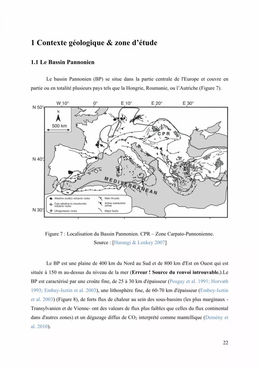
Le bassin Pannonien (BP) se situe dans la partie centrale de l'Europe et couvre en

partie ou en totalité plusieurs pays tels que la Hongrie, Roumanie, ou l’Autriche (Figure 7).

Figure 7 : Localisation du Bassin Pannonien. CPR – Zone Carpato-Pannonienne.

Source : [Harangi & Lenkey 2007]

Le BP est une plaine de 400 km du Nord au Sud et de 800 km d'Est en Ouest qui est

située à 150 m au-dessus du niveau de la mer (Erreur ! Source du renvoi introuvable.).Le

BP est caractérisé par une croûte fine, de 25 à 30 km d'épaisseur (Posgay et al. 1991; Horvath

1993; Embey-Isztin et al. 2003), une lithosphère fine, de 60-70 km d'épaisseur (Embey-Isztin

et al. 2003) (Figure 8), de forts flux de chaleur au sein des sous-bassins (les plus marginaux -

Transylvanien et de Vienne- ont des valeurs de flux plus faibles que celles du flux continental

dans d'autres zones) et un dégazage diffus de CO2 interprété comme mantellique (Demény et

al. 2010).

23

Figure 8 : Épaisseurs crustale (a) et lithosphérique (b) du BP. Source [Huismans et al. 2002]

D'un point de vue géologique le BP est entouré à l'Ouest par les Alpes, au Sud par les

Alpes Dinarides et au Nord et à l'Est par l'Arc des Carpates (ceinture de plissements et de

chevauchements, Hidas et al. 2010). Il est séparé en deux unités tectoniques majeures qui sont

l'ALCAPA (Alpes-Carpates-Pannonie) au Nord et Tisza-Dacia au Sud. Entre ces deux unités

majeures se situe la Mid Hungarian Zone que nous décrirons plus loin dans ce chapitre

(Figure 9).

Figure 9 : Unités tectoniques majeures du BP. Source [Harangi & Lenkey 2007]

24

1.2 La géodynamique locale

1.2.1 Historique

La mise en place du substratum du BP a commencée, au Carbonifère moyen, lors de la

collision entre les continents Laurentia (au Nord) et Gondwana (au Sud). Cette collision, à

l'origine de la formation de la Pangée, a provoqué la fermeture de la Téthys, la formation

d'une suture le long de la marge européenne (et à l'Ouest du futur BP) et le métamorphisme de

la roche paléozoïque (Figure 10).

Figure 10 : Fermeture de la Téthys à l'origine de la formation du super continent, La Pangée. Sources : [a - Un essai de schématisation des grands traits de l'histoire géologique de la Terre;

b – Geowiki]

La réouverture de la Téthys, de la fin du Permien à la fin du Jurassique, va entrainer la

mise en place d'une zone de rifting, la formation de grabens (Dolton 2006; Horvath & Tari

1999), de plateformes et de bassins sédimentaires (Figure 11).

La Téthys se refermera, entre le Jurassique et le Crétacé inférieur, par la convergence

entre la plaque Européenne et des fragments crustaux provenant de la plaque Africaine. Cette

convergence va entrainer le développement d'une zone de subduction et la mise en place de

volcanisme calco-alcalin.

a

b a

25

Figure 11 : Évolution de la Réouverture de la Téthys (Permo-Trias à Jurassique).

Source : [Delacou 2004]

La première compression majeure a lieu entre la fin du Crétacé et le Paléocène. C'est elle

qui sera à l'origine du premier épaississement crustal de la formation des Alpes, du

métamorphisme de haute pression (Delacou 2004) et de la formation de l'océan Parathétys

(Figure 12). Le BP reposera par la suite, sur les plissements de l'orogénèse alpine (Dolton

2006).

26

Figure 12 : Collision entre la plaque Européenne et des fragments crustaux provenant de la plaque Africaine. Source : [Delacou 2004]

A partir de l'Éocène, la deuxième phase compressive de la formation des Alpes a lieu.

Cette deuxième phase compressive va donner lieu à un épaississement crustal important et à

la formation d'une profonde racine lithosphérique (Delacou 2004) (Figure 13).

Figure 13 : Évolution de la collision Europe / fragments africain entre le Crétacé et l'Éocène. Source : [Delacou 2004]

Entre l'Éocène et le début de l'Oligocène, la convergence a poussé les blocs Apulien,

Pelso et Tisza plus loin dans la plaque européenne provoquant ainsi des transpressions et

rotations de blocs et le développement du Bassin Paléogène Hongrois (Figure 14).

Figure 14 : Évolution de la collision Europe / fragments africain à l'Éocène.

Source : [Delacou 2004]

27

Au milieu de l'Oligocène, il y a transport de l'ALCAPA dans les Carpates (Hidas et al.

2010); l'ALCAPA est donc séparé du Sud des Alpes et va migrer vers l'Est avec une rotation

antihoraire. Un ensemble de bassins va se développer dans la partie centrale du bassin

Paléogène entre l'Éocène et le Miocène supérieur (Figure 15).

Entre la fin de l'Oligocène et le début du Miocène un fort amincissement ante-rift associé

à une compression N-S à NO-SE a lieu ainsi qu'une fusion importante dans le manteau

antérieurement métasomatisé (Hidas et al. 2010).

Figure 15 : Évolution de la collision Europe / fragments africain entre l’Oligocène et le présent. Source : [Delacou 2004]

28

A la même époque, les rotations horaires du bloc Tisza-Dacia et antihoraires du bloc

ALCAPA vont conduire à la formation de la Mid Hungarian Zone (MHZ) (Figure 16). La

MHZ a encore subi de fortes déformations il y 16 Ma, car pendant cette période, la collision

ALCAPA/Europe va provoquer une déformation extensive entre le bloc ALCAPA en rotation

et le bloc Tisza-Dacia (Kovács & Szabó 2008).

Figure 16 : Structure lithosphérique du BP définie grâce à plusieurs aquisitions sismiques grand-angle et des profils de sismique réflexion. Source : [Środa et al. 2006]

1.2.2 Thermomécanique associée

Les modèles numériques ont montré que la création d'une racine lithosphérique va

entrainer une force gravitaire verticale à l'origine d'une extension lithosphérique adjacente

(Michon 2001) (Figure 17).

29

Figure 17 : Modèle expliquant l'extension lithosphérique à proximité d'une racine lithosphérique ; Source : [Michon 2001]

De plus, cette force gravitaire verticale va également entrainer un fluage

asthénosphérique (Figure 18) vers les régions périphériques ce qui peut provoquer une érosion

thermomécanique de la limite Lithosphère/Asthénosphère, une accentuation du volcanisme

par fusion du manteau lithosphérique et un déséquilibre isostatique entrainant la surrection de

l'ensemble de la lithosphère (Michon 2001).

Figure 18 : Modèles expliquant le fluage lithosphérique lié à une force gravitaire verticale. a-

fluage asthénosphérique; b- érosion thermomécanique de la limite lithosphère/asthénosphère.

Source : [Michon 2001]

a b

30

1.2.3 Volcanisme et flux de chaleur

Le développement Néogène du BP a été accompagné d'une activité volcanique

répétitive et intensive (Huismans et al. 2002). Au Miocène inférieur, il y a des dépôts

d'ignimbrite et de tufs, notamment au niveau de la MHZ (Figure 19). Ces dépôts pourraient

être liés aux mouvements décrochants.

Au Miocène moyen et jusqu'à récemment (16,5-2 Ma), des édifices calco-alcalins sont

mis en place dans le BP. Les roches calco-alcalines sont présentes dans la partie Est

(affleurements), centrale (enfouies), mais aussi de manière sporadique dans l’ouest du bassin

Pannonien. Ces roches mafiques calco-alcaline (SiO2 = 49-57 wt. % ; MgO > 3 wt. %) ont des

Mg-number (Mg/Mg + Fe) de 0,5-0,6 suggérant divers degrés de différenciation par

cristallisation fractionnée. Ces roches sont principalement de composition andésitique ou

dacitique et montrent des caractéristiques chimiques typiques de magmas de zone de

subduction. De ce fait, la formation de l’arc de Carpates a été interprétée comme une

conséquence des processus de subduction (Szabo et al. 1992; Downes & Vaselli 1995; Bleahu

et al. 1973; Balla 1981). Dans les zones de subduction actuelles, les arcs volcaniques se

développent à environ 110-170 km au-dessus de la plaque plongeante et la largeur de l'arc

volcanique est fonction de l'angle de subduction (Tatsumi & Eggins 1995). La plaque

océanique en subduction subit du métamorphisme et de la déshydratation en continu. Les

phases fluides libérées par les réactions de déshydratation entrent dans la partie inférieure du

coin de manteau et forment des phases hydratées telles que l’amphibole et la phlogopite

(Pearce & Peate 1995). La déstabilisation de ces minéraux hydratés à environ 110 et 170 km

de profondeur, libère des fluides qui migrent vers le manteau supérieur, diminuent le solidus

et initient la fusion partielle. La répartition spatiale des formations volcaniques et la largeur

des complexes volcaniques suggèrent une subduction relativement peu profonde (30-40°)

associée au volcanisme de la partie ouest de l'arc des Carpates, alors que la subduction située

à l’Est est relativement profonde (50 -60°). Cependant, il y a des problèmes notables avec le

modèle classique de magmatisme de subduction lorsqu'il est appliqué à cette région: (1)

l'activité volcanique calco-alcaline a commencé quand la subduction de la plaque océanique a

cessé, comme indiqué par le raccourcissement final dans les Carpates extérieures (Jiricek

1979). Ainsi, cette activité volcanique peut être considérée comme post-collisionnelle

(Seghedi et al. 1998). (2) Les roches volcaniques calco-alcalines se trouvent également dans

la partie centrale du bassin Pannonien, où elles sont majoritairement recouvertes par une

31

séquence sédimentaire d’âge Miocène à Quaternaire (Pécskay et al. 1995). (3) Il y a une

migration progressive du volcanisme du NO au SE, le long des Carpathes de l'Est ; cette

migration est accompagnée d’une baisse du volume des magmas éruptés (Pécskay et al.

1995). (4) La première éruption a eu lieu en même temps que la phase syn-rift du bassin

Pannonien.

Figure 19 : Localisation des volcanismes calco-alcalins et alcalins.

Source : [Harangi & Lenkey 2007]

L'activité volcanique du Néogène dans la région Carpato-Pannonienne (CPR) est

étroitement liée à l'évolution tectonique de la région. Durant le Crétacé et le Paléogène, la

subduction de la lithosphère océanique n'a pas abouti à la production directe de volcanisme

calco-alcalin du fait du champ de contraintes compressives et de la présence d'une épaisse

lithosphère (Harangi & Lenkey 2007). Néanmoins, ce processus a joué un rôle important dans

la génération de magmas. La déshydratation du slab a métasomatisé le coin de manteau,

abaissant ainsi la température de fusion. Les magmas n’ont atteint la surface qu'au début de

l’extension lithosphérique, au début du Miocène (19-21 Ma).

32

Le volume du volcanisme calco-alcalin a été estimé à ~1400km3. De la fin du

Miocène à récemment, des basaltes alcalins probablement liés à la décompression du manteau

peu profond sont mis en place dans des zones diffuses à l'intérieur du BP (Figure 20).

Figure 20 : Echelle des temps géologiques décrivant les principaux évènements tectoniques et volcaniques de la formation du bassin Pannonien. Source : [Modifié d’après Harangi & Lenkey, 2007]

33

La première apparition des basaltes alcalins est contemporaine à la deuxième phase de

rifting (11,5 Ma) et à un upwelling de manteau lithosphérique. La plus grande quantité de

basaltes alcalins se situe dans les Balatons Highland et dans le Bassin de Graz qui se situe

légèrement à l'Ouest du centre d'amincissement maximum du BP. Les auteurs décrivant les

basaltes alcalins semblent s'accorder avec une température asthénosphérique pas plus élevée

que la normale (aucune anomalie thermique), notamment grâce aux faibles volumes de

basaltes émis et aux faibles taux d'éruption.

Les champs volcaniques basaltiques du BP se présentent sous forme de petits édifices

monogéniques distribués individuellement ou en petits regroupements (Jankovics et al. 2012).

On trouve donc des cônes de scories, des maars, des cônes de tufs, des anneaux de tufs ou des

petits champs de lave. Les coulées de lave font parfois jusqu'à 2000-3000 mètres d'épaisseur

dans des zones structurales spécifiques (Nagymarosy & Hamor 2012). Le Bakony Balaton

Highland Volcanic Field (BBHVF) compte par exemple, 150 à 200 centres éruptifs. Cette

zone sera décrite plus amplement à la fin de ce chapitre, puisqu’elle constitue notre zone

d’étude.

1.3 Le bassin sédimentaire

1.3.1 Mise en place du Bassin Pannonien

Historique

Le BP Néogène repose sur des strates très déformées des Carpates internes et sur les

bassins du Paléocène. La formation du BP a commencé il y a 18 Ma (Début Miocène) par une

subduction roll-back (la limite marquant le contact entre la plaque subductée et la plaque

subductante va reculer en direction de la plaque subductée) de la plaque Européenne le long

du front des Carpates (Figure 21a), qui va être compensée par un mouvement en direction de

l'Est et avec une pression continue de la lithosphère pannonienne ante-rift (Figure 21b). La

subduction roll-back va faciliter l'extension à l'intérieur du bassin (Corver et al. 2009).

34

Figure 21 : a- Subduction roll-back; b- Extension du BP liée à la subduction.

Source : [Huismans et al. 2002; Corver et al. 2009]

La première phase de rifting correspond à du rifting passif lié à l'extension back-arc

(Dolton 2006; Huismans et al. 2002; Degi et al. 2010). Elle est représentée par une période

active de formation de failles en extension dans la partie interne du continent (Corver et al.

2009). Elle va être la cause de l'ouverture de bassins en pull-appart sur les bords du BP ; dans

un régime transtensionnel entre 17,5 et 14,5 Ma et d'extension pure entre 16,5 et 14 Ma. Elle

est caractérisée par une subsidence tectonique rapide et est enregistrée partout dans le BP

(Corver et al. 2009). Ce rifting a aminci fortement la lithosphère de la partie centrale du BP

(Huismans et al. 2002). On notera que l'extension du BP est diachronique et qu'elle a

commencé par les parties les plus externes. L'extension crustale ainsi que l'amincissement

lithosphérique vont contrôler la subsidence entre 17 et 12 Ma (Horvath et al. 1988). La

direction de la plupart des failles transformantes (WSW-ENE) correspond à l'axe principal de

l'étirement maximal (Horváth & Rumpler 1984); elles sont perpendiculaires au principal front

de subduction. L'extension de la zone interne a été accompagnée par de petites rotations de

blocs individuels faillés. La principale période d'extension a été interrompue par de courtes

ou longues inversions, c'est-à-dire par des périodes durant lesquelles la compression et le

soulèvement étaient dominants. Une explication possible pour cet arrêt dans la subsidence

pourrait être qu'à la fin du Sarmatien, la totalité de la lithosphère océanique disponible pour la

subduction a été enfouie dans l'Est des Carpates. Ceci pourrait donc être le début de la

collision entre les continents Tisza-Dacia et la plateforme européenne.

Comme constaté par Royden et al. (1982), la principale direction de l'extension du BP

s'est produite le long de fractures OSO-ENE. Ceci a été compensé par un raccourcissement

contemporain de l'Est des Carpates. L'extension de la partie profonde de la lithosphère ductile

a b

35

du BP peut s'expliquer par de la déformation plastique et de l'étirement alors que l'extension

de la partie supérieure de la lithosphère s'est faite par déformation tectonique cassante. Dans

la partie supérieure de la lithosphère deux mécanismes majeurs sont responsables de la

formation des bassins profonds:

- L'extension le long de faibles angles de failles normales. La formation de ces failles

est fortement liée au développement de complexes métamorphiques (Crittenden et al.

1980; Lister & Snoke 1984). En raison de l'updoming et du soulèvement du complexe

métamorphique, les nappes vont glisser vers le bas entrainant un amincissement de la

croûte et la formation de bassins profonds. Les mesures par traces de fission ont

montré que le soulèvement et l'exhumation du complexe métamorphique ont eu lieu,

dans la majorité des cas, durant le Badénien, c'est-à-dire durant la principale phase de

la subsidence syn-rift au cours de la première moitié du milieu Miocène sur le

territoire hongrois (Dunkl et al. 1994; Dunkl, I. and Demény 1997).

- L'activité transformante des failles. Le rifting général a lieu le long de systèmes de

failles transformantes. Celles-ci sont répandues en Hongrie; leur existence a été

prouvée par de nombreuses coupes sismiques (Horváth & Rumpler 1984). Une forte

concentration de failles transformantes est présente le long de la Mid Hungarian Zone.

La formation des bassins profonds a lieu entre le début et le milieu du Miocène. Le

développement de ces bassins peut être attribué à la première phase syn-rift. Dans les stades

plus tardifs, ces dépressions ont été regroupées en une série de sous-bassins connectés ;

l'aspect uniforme de l'actuel BP n'a été atteint que pendant l'importante évolution structurale

de la fin du Miocène c'est-à-dire, dans la phase thermique de la formation du bassin. Les

sédiments déposés durant la phase syn-rift sont principalement d'origine marine. La fin de la

première phase de rifting a eu lieu il y a 14 Ma. Cependant, un échappement vers l'Est ainsi

qu'un décrochement continu sont toujours présent après 14 Ma. Le développement du BP a

été accompagné par une forte activité magmatique. Il y a 11,5 Ma a eu lieu une compression

E-O à l'origine d'un uplift et d'une érosion importante (visible grâce à un hiatus temporel). La

deuxième phase de rifting (ou phase post-rift) a eu lieu entre 11,5 et 8 Ma et n'est visible que

dans les parties centrales du BP. Elle est associée à une remontée convective d'asthénosphère

qui serait liée à l'étirement et à l'amincissement de la lithosphère pannonienne et serait

contemporaine à la construction de l'Arc dans l'Est des Carpates (Huismans et al. 2002;

Corver et al. 2009).

36

La phase thermique a eu lieu de 12 Ma à récemment (Horvath et al. 1988). Elle

présente seulement des extensions locales et mineures (fluage de la lithosphère qui contrôle la

subsidence). Elle est caractérisée par un affaissement thermique sans faille majeure, même

dans la partie interne du continent. Cette relaxation thermique est cependant à l'origine de la

relaxation générale, de la subsidence post-rift et de la continuité de la compression dans l'Est

des Carpates. L'extension majeure a quasiment cessé à la fin du Miocène.

La subsidence thermique et la sédimentation rapide dans la seconde phase de rifting

ont donné lieu à un dépôt relativement "plat" des strates. Les sédiments post-rift ne sont pas

perturbés et reposent en discordance sur les séquences syn-rift dans la plupart des sous-

bassins et sur les roches du socle au niveau des horsts.

Figure 22 : a- Deuxième phase de rifting associée à l'épisode compressif; b- Extension et compression contemporaine + remontée convective d'asthénosphère. Source : [Huismans et al.

2002; Corver et al. 2009]

La période post-rift est marquée par deux événements compressifs. Les deux phases

sont associées à la réactivation de failles et à des inversions structurales à des échelles locales

et régionales. Le premier événement compressif a eu lieu juste après la phase syn-rift (11-8

Ma, Figure 22) tandis que le deuxième événement a commencé au cours du Pliocène et a

continué jusqu'à récemment (~6-0 Ma) (Corver et al. 2009).

Le BP n'est pas entièrement uniforme; il y a des bassins très profonds (>7000m) et

d’autres peu profonds (<1000m). Sclater et al. (1980), Nagymarosy (1981) and Horvath et al.

(1988) ont montré que le taux de subsidence et le taux de sédimentation n'étaient constants ni

dans l'espace, ni dans le temps, pendant l’évolution du BP.

a b

37

La formation du BP actuel s'est achevée au Pléistocène (Hidas et al. 2010); cependant,

le BP est toujours affecté d'un champ de contraintes actif (Huismans et al. 2002) et d'un flux

de chaleur important qui montrent que la limite lithosphère/asthénosphère est toujours en

position élevée (Nagymarosy & Hamor 2012). Pendant le Miocène, la limite

lithosphère/asthénosphère devait être dans une position encore plus élevée qu'actuellement

pour deux raisons possibles :

- L'effet roll-back de la lithosphère océanique subductée dans l'Est des Carpates, tirée en

direction du N et du N-E, va entrainer l'aspiration de la lithosphère plastique profonde

en direction de la zone de subduction. Ceci a pu provoquer un étirement considérable

de la lithosphère profonde.

- En accord avec Andrews & Sleep (1974) la lithosphère subductée génère un flux

convectif dans l'asthénosphère et le flux engendré peut avoir érodé thermiquement la

lithosphère mantellique de la microplaque intra-carpatienne et peut être même la

croûte inférieure.

Il semble clair que dans les deux cas, la subduction qui était une conséquence de

l'extrusion des microplaques ALCAPA et Tisza-Dacia pendant le Paléogène (Balla 1984;

Csontos et al. 1992), a été un des moteurs dans le développement de la subsidence générale du

BP (Figure 23).

L'évolution du BP à la fin du Miocène a été caractérisée par la poursuite de la

réactivation tectonique. Cela comprend l'inversion des failles normales déjà formées, le

soulèvement des flancs Est et Ouest du BP, la continuité de la subsidence et la réactivation

des failles décrochantes dans la partie centrale du BP (Corver et al. 2009).

38

Figure 23 : Modèle géodynamique 3D de la formation du BP au début du Miocène (16-18 Ma). Source : [Horváth et al. 2015]

1.3.2 Le système pétrolier du bassin

Les roches réservoirs du BP sont variées en âges et en lithologies. Selon Dank (1987),

les réservoirs du Néogène comptent 61% des ressources de pétrole découvertes en Hongrie;

les unités Mésozoïque et Paléozoïques comptent pour 33% et les roches Paléogènes comptent

pour 7%. Des études plus récentes de Kókai (1994) indiquent que 62% de la production de

pétrole provient des roches sédimentaires Cénozoïques et 24% provient des carbonates

Mésozoïque. 70% de la production de gaz naturel provient des réservoirs Cénozoïques

(Dolton 2006).

Les roches Néogènes sont le principal réservoir de la province du BP et représentent

plus de 80% de la production de tous les réservoirs. Dans ces roches Néogènes, les grès

comptent 95% de la production et 90% de ces grès sont du Miocène, les autres étant du

Pliocène.

39

La maturation de la matière organique est supposée avoir eu lieu pendant le flux de

chaleur maximum à la fin du Miocène ou au Pliocène (6-2 Ma). Comme constaté par Ziegler

and Roure (1996), les séries Oligocènes dans le BP comptent d’importants réservoirs

d’hydrocarbures. Les roches Néogène d'âge Miocène sont considérées comme étant la

principale source d’huile et de gaz de la région (Dolton 2006) (Figure 24).

Figure 24 : Histoire de l'enfouissement de la plaine Néogène hongroise.

Source : [Dolton 2006]

La moyenne du gradient géothermique du système pannonien est d'environ

3,6°C/100m et excède parfois 5,8°C/100m. Étant donné ce fort gradient géothermal, les

roches mères fournissent des sources pour les huiles et les gaz à des profondeurs relativement

faibles. Bien que le flux de chaleur et la profondeur de la fenêtre à huile soient variables

régionalement, les investigations suggèrent généralement le début de la génération thermique,

dans la majorité du système, à environ 2000m pour une huile immature et à environ 2500m

40

pour une huile mature. Les roches situées à environ 5000m de profondeur sont typiquement

dans le domaine de la génération de gaz (fenêtre à gaz) (Dolton 2006). La génération d’huile

dans les sédiments Néogènes a débuté entre 8 et 5 Ma et a progressé de telle sorte que les

sédiments situés à une profondeur de 4-5 km sont passés par la fenêtre à huile. Les 2-3

kilomètres supérieurs de roches sédimentaires Néogènes sont immatures dans tout le bassin, et

par conséquent, les lits riches en matière organique du Pannonien supérieur ne sont pas

suffisamment enfouis pour générer des hydrocarbures. Cependant, dans plusieurs zones, les

jeunes sédiments contiennent des gaz d'hydrocarbures secs qui sont composés de méthane

isotopiquement léger, biogénique ou diagénétique provenant de sources humiques (Dolton

2006).

Les réservoirs d’huile et de gaz sont souvent situés dans des roches thermiquement

immatures au-dessus des sommets du socle ou latéralement écartés des zones de production.

L’huile est stockée à des profondeurs généralement inférieures à 3000m avec une majorité

entre 1000 et 1500m (Figure 25a). Le gaz est, quant à lui, stocké à des profondeurs

généralement inférieures à 3500m avec une majorité entre 1000 et 2500m (Figure 25b).

Ceci indique des migrations verticales et latérales omniprésentes. Les champs d’huile

sont généralement situés sur les périmètres des zones de production de gaz, ce qui suggère

que les gaz peuvent avoir déplacé l’huile latéralement (Dolton 2006).

Une structure anticlinale formée dans les couches Néogènes, offre potentiellement de

bons pièges pour les hydrocarbures qui migrent vers le haut depuis des roches plus profondes

datant du Miocène. Toutefois, une part importante (~1-2 km) de la jeune séquence

sédimentaire a été érodée et plusieurs pièges ont probablement perdu leurs hydrocarbures

(Corver et al. 2009).

41

Figure 25 : a- Huile découverte par zones de profondeurs et b- Gaz découvert par zones de profondeurs. Source : [Dolton 2006]

Pendant la première phase de rifting, les types de pièges se situent principalement dans

les blocs basculés et les horsts, tandis que durant la deuxième phase de rifting une plus grande

variété de types de pièges s'est développée selon le degré de subsidence, de

soulèvement/inversion et de compression (Corver et al. 2009) (Figure 26).

a

b

42

Figure 26 : Coupe schématique montrant le système pétrolier dans le bassin Néogène. Source : [Corver et al. 2009]

Dans l'ensemble du BP, les réservoirs de gaz contiennent généralement des quantités

importantes de CO2 interprétées par certains auteurs comme provenant de la décomposition

des carbonates dans le socle rocheux profondément enfouis ou par d’autres comme provenant

du manteau sous-Pannonien (Sherwood Lollar et al. 1997). La gamme des teneurs en CO2 va

de 0,5 à 99,5% avec une moyenne de 28%. Dans le bassin du Danube, en particulier, la teneur

en CO2 du gaz naturel compromet toute rentabilité (Dolton 2006).

1.4 La Bakony Balaton Highland

1.4.1 Contexte géologique de la zone d’étude

Pour notre étude nous nous sommes focalisés sur la zone volcanique de le BBHVF

(Bakony Balaton Highland Volcanic Field) où nous avons échantillonné quatre édifices

volcaniques : Füzes-tó, Mindszentkálla, Szentbékkálla et Szigliget (Figure 27).

43

Figure 27 : Cartographie des zones d’échantillonnage

Le BBHVF est localisée à l'Ouest du BP (Ouest de la Hongrie) et sur la rive Nord du

lac Balaton. D'un point de vue géologique, elle est située sur la partie sud de la microplaque

Alcapa. Le BBHVF appartient à la zone centrale de la Chaîne Transdanubienne, qui est

corrélée avec les nappes austro-alpines supérieures de l'orogénèse des Alpes de l'Est (Majoros

1983; Tari 1991; Kazmer & Kovacs 1985). Le socle des champs volcaniques est constitué de

roches paléozoïques, de schistes siluriens, de sédiments rouge permiens (Császár & Lelkesné

Felvári 1999) et d'une épaisse séquence de carbonates mésozoïques (Budai & Voros 1992;

Haas et al. 1999), qui a été déposée sur l'unité Alpine (SO de la zone) et a été transportée en

direction du N-E par le mouvement de la microplaque Alcapa pendant l'évolution

géodynamique du BP. Ce socle forme maintenant une structure anticlinale à large échelle

d'origine Eoalpine dans la zone Transdanubienne centrale et elle est localement recouverte de

sédiments (Horvath 1993; Tari et al. 1992). Les sédiments Cénozoïques ont été déposés dans

des bassins sédimentaires locaux sur une discordance régionale liée à l'érosion (Müller et al.

1999; Muller & Magyar 1992). Au Néogène et juste avant le début du volcanisme, le lac

Pannonien occupait la majeur partie du BP. Les sédiments lacustres, mudstones et les marnes

issues de l'eau saumâtre du lac Pannonien sont très répandues dans le bassin (Jambor 1980;

Gulyás 2001). Juste avant le début du volcanisme, la partie Ouest du BP formait une plaine

alluviale avec des sédiments non consolidés et chargés en eau (Kázmér 1990).

44

1.4.2 Le volcanisme basaltique alcalin

Les centres volcaniques de le BBHVF ont été actifs entre 7.96 et 2.61 Ma, (Borsy et

al. 1986; Balogh & Németh 2005; Balogh & Pécskay 2001; Balogh et al. 1980; Wijbrans et al.

2007) et ont produit principalement des roches basaltiques alcalines (Szabo et al. 1992;

Embey-isztin et al. 1993). Le BBHVF compte environ 50 volcans basaltiques dans une zone

relativement petite (~ 3500 km²) ; cependant, le nombre d'évents peut être très supérieur du

fait de l'existence de complexes volcaniques et de volcans imbriqués (Martin et al. 2003). Le

volcanisme basaltique alcalin dans l'Ouest du bassin était principalement subaérien et de type

intracontinental. Cependant, de grandes quantités d'eau peu profonde peuvent avoir été

présentes durant les éruptions, celles-ci auraient vraisemblablement conduit à la formation des

volcans émergents (Kokelaar 1983; White & Houghton 2000). Après l'arrêt du volcanisme, la

sédimentation fluviale/alluviale s’est répandue dans l'Ouest du bassin. Tous les types de

volcans peuvent être trouvés dans la partie Ouest du bassin et dans le BBHVF. On y retrouve

des formations géomorphologiques proéminentes circulaires ou des buttes couvertes de lave.

Ces formations circulaires sont généralement liées à des volcans phréatomagmatiques, comme

à des structures de maar ou des anneaux de tufs (Nemeth et al. 2003). Le lac Balaton quant à

lui est récent et son histoire remonte seulement à 17000-15000 ans (Cserny & Corrada 1989;

Tullner & Cserny 2003).

1.4.3 Les édifices volcaniques étudiés

Szentbékkálla

Le village de Szentbékkálla est situé au milieu de le BBHVF, à environ 10km au Nord

du lac Balaton (N 46°53'26.30'' et E 17°33'52.66'', altitude: 150-200m).

La cartographie de la région de Szentbékkálla révèle de petits volumes de dépôts de

flux pyroclastiques, supposés être le résultat d'éruptions explosives phréatomagmatiques. Des

lits de tufs à lapilli massifs, non triés et grossiers alternent avec des lits entrecroisés à matrices

riches en blocs. Le corps principal de la séquence pyroclastique est constitué de lits de tufs à

lapilli gris, massifs et compacts. Il n'y a aucune évidence de classement, de structures

sédimentaires bien développées, ou de soudure dans cette unité. Le tuf à lapilli contient une

grande quantité de xénolites ultramafiques de forme arrondie à semi-arrondie, des olivines

45

fracturées/cassées et des xénocristaux de clinopyroxène (Cpx) sans aucune observation

d'accumulation (Martin & Németh 2004). Les fragments juvéniles de tufs à lapilli et de tufs de

Szentbékkálla vont généralement de la phono-téphrite à la téphri-phonolite (Nemeth et al.

1999). De petites aiguilles de verre, altérées, et de couleur claire montrent des compositions

de dacite/trachydacite et andésite basaltique (Nemeth et al. 1999).

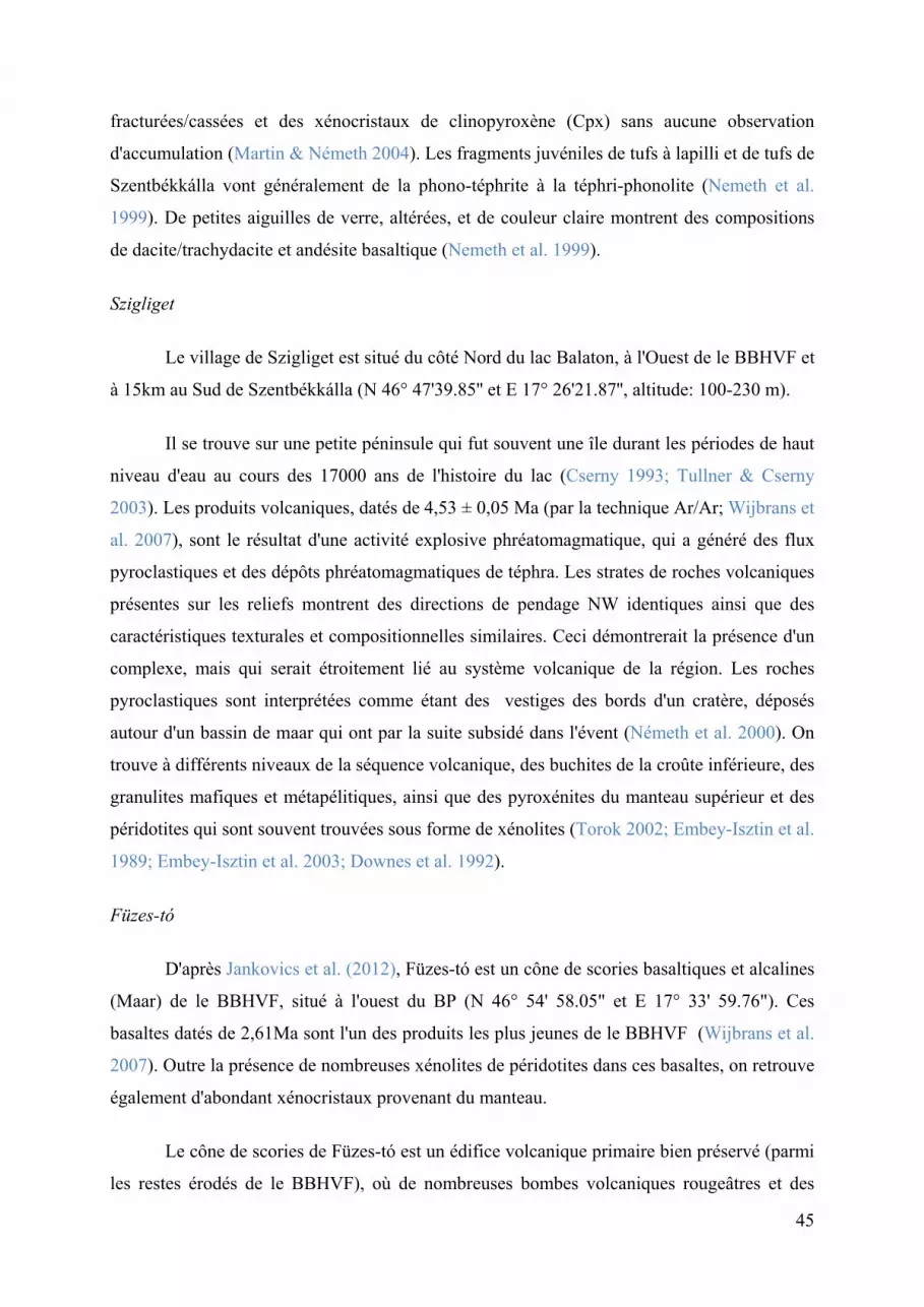
Szigliget

Le village de Szigliget est situé du côté Nord du lac Balaton, à l'Ouest de le BBHVF et

à 15km au Sud de Szentbékkálla (N 46° 47'39.85'' et E 17° 26'21.87'', altitude: 100-230 m).

Il se trouve sur une petite péninsule qui fut souvent une île durant les périodes de haut

niveau d'eau au cours des 17000 ans de l'histoire du lac (Cserny 1993; Tullner & Cserny

2003). Les produits volcaniques, datés de 4,53 ± 0,05 Ma (par la technique Ar/Ar; Wijbrans et

al. 2007), sont le résultat d'une activité explosive phréatomagmatique, qui a généré des flux

pyroclastiques et des dépôts phréatomagmatiques de téphra. Les strates de roches volcaniques

présentes sur les reliefs montrent des directions de pendage NW identiques ainsi que des

caractéristiques texturales et compositionnelles similaires. Ceci démontrerait la présence d'un

complexe, mais qui serait étroitement lié au système volcanique de la région. Les roches

pyroclastiques sont interprétées comme étant des vestiges des bords d'un cratère, déposés

autour d'un bassin de maar qui ont par la suite subsidé dans l'évent (Németh et al. 2000). On

trouve à différents niveaux de la séquence volcanique, des buchites de la croûte inférieure, des

granulites mafiques et métapélitiques, ainsi que des pyroxénites du manteau supérieur et des

péridotites qui sont souvent trouvées sous forme de xénolites (Torok 2002; Embey-Isztin et al.

1989; Embey-Isztin et al. 2003; Downes et al. 1992).

Füzes-tó

D'après Jankovics et al. (2012), Füzes-tó est un cône de scories basaltiques et alcalines

(Maar) de le BBHVF, situé à l'ouest du BP (N 46° 54' 58.05" et E 17° 33' 59.76"). Ces

basaltes datés de 2,61Ma sont l'un des produits les plus jeunes de le BBHVF (Wijbrans et al.

2007). Outre la présence de nombreuses xénolites de péridotites dans ces basaltes, on retrouve

également d'abondant xénocristaux provenant du manteau.

Le cône de scories de Füzes-tó est un édifice volcanique primaire bien préservé (parmi

les restes érodés de le BBHVF), où de nombreuses bombes volcaniques rougeâtres et des

46

fragments de différentes tailles et formes peuvent être trouvés : des bombes en fuseau,

scoriacées ou en croûte de pain ainsi que des pyroclastites agglutinés (Jankovics et al. 2012).

Les bombes contiennent souvent des xénolites denses et ultramafiques du manteau supérieur

qui sont souvent plus ou moins altérés. Des fragments massifs de lave, qui contiennent de

petits fragments de xénolites altérés, peuvent être également trouvés.

Mindszentkálla

D'après Nemeth et al. (2003), Kereki-hegy est situé à 1 km au sud-est de

Mindszentkálla (N 46° 51' 46.40" et E 17° 32' 36.31"; altitude 171m) et se présente comme

une petite colline allongée (~ 150 m du nord au sud) d'environ 60 mètres au-dessus du

plancher du bassin Káli. Les formations carbonatées du Trias inférieur affleurent à la surface à

proximité de la zone (Budai & Csillag 1998; Budai et al. 1999). Dans le voisinage immédiat

de la colline, des unités silicoclastiques du Néogène, épaisses de quelques mètres, ont été

cartographiés (Budai et al. 1999) mais leur existence fait encore l'objet d'un débat. En dépit de

cela, l'ancienne cartographie géologique décrit des prismes de basalte à cet endroit (Vitalis

1911), bien que de nouvelles cartographie n'aient pas été en mesure de confirmer cette

information (Budai et al. 1999; Nemeth et al. 2003).

Les lits pyroclastiques ont une forte inclinaison (60°) et plongent vers l'Est, ce qui

diffère des tendances tectoniques connus dans la région ainsi que du litage subhorizontal des

unités rocheuses pré-volcaniques que le diatrème recoupe (Budai et al. 1999). Les roches

pyroclastiques de cette zone sont riches en échardes de verre volcaniques (Nemeth et al.

2003), qui sont de formes allongées à polyédriques et modérément microvésiculaires. La

combinaison de ces caractéristiques suggèrent que l'interaction eau-magma était le style de

fragmentation dominant de leur formation (Nemeth et al. 2003). D'un point de vue textural et

compositionnel les parties litées et massives des roches pyroclastiques ne diffèrent pas les

unes des autres (Nemeth et al. 2003). Kereki-hegy est interprété comme un diatrème

profondément érodé, dans lequel les niveaux profonds du diatrème sont exposés. La

couverture sédimentaire Néogène aurait été encore intacte au cours de l'éruption du Kereki-

hegy (Nemeth et al. 2003). Lors des épisodes volcaniques, des enclaves mantelliques et

crustales ont été remontées à la surface.

47

2 Les xénolites de le BBHVF

Des xénolites mantelliques ultramafiques peuvent être trouvés dans des laves

basanitiques et dans des pyroclastes volcaniques dans six zones de le BBHVF (Tihany,

Bondoró Hill, Füzes-tó, Szentbékkálla, Mindszentkálla, Szigliget) (Figure 28).

Ces xénolites sont d’origine lithosphérique et dans quelques cas d’origine

asthénosphérique. Comme l’éruption des basaltes alcalins est postérieure aux principaux

évènements tectoniques dans la zone Carpato-Pannonienne, les xénolites ont enregistré les

effets de ces évènements, ce qui inclus la déformation (Falus 2004; Falus et al. 2004; Falus et

al. 2008; Hidas et al. 2007), le métasomatisme (Bali et al. 2002; Enikő Bali et al. 2008; Szabó

et al. 2009; Hidas et al. 2010) et l’extraction de magmas (Bali et al. 2002; Bali et al. 2008;

Szabó et al. 2009; Hidas et al. 2010). Ces xénolites peuvent donc être utilisés comme outils

pour connaitre l’évolution du bloc lithosphérique. Les péridotites sont des résidus

mantelliques montrant des preuves texturales et géochimiques d’une histoire complexe

alternant des épisodes de fusion et de recristallisation (Szabó et al. 2004). Les xénolites

mantelliques contiennent également des phases hydratées (pargasites, kaersutites et rarement

phlogopites) qui prouvent un métasomatisme modal du manteau sous Pannonien (Embey-

Isztin 1976; Szabo & Taylor 1994; Szabó et al. 2004; Szabó et al. 2009).

La plupart des xénolites sont des lherzolites à spinelles, ou des harzburgites,

clinopyroxenites, orthopyroxenites, wehrlites, websterites ou parfois, des xénolites

composites (Szabo et al. 2010). La texture la plus fréquement observée est équigranulaire

(Embey-Isztin et al. 1989; Downes et al. 1992; Downes & Vaselli 1995; Szabó et al. 2004),

mais des xénolites protogranulaires ou porphyroclastiques peuvent également être trouvés en

plus faible proportion. Des textures poecilitiques, tabulaires et mylonitiques sont également

présentes dans les xénolites dans différentes proportions selon les zones volcaniques (Figure

28). Les péridotites présentes dans les basaltes alcalins de le BBHVF ont des compositions sur

roches totales allant de 37-45 wt. % MgO, 1.0-3.5 wt. % CaO et Al2O3, et 0.02-0.14 wt. %

TiO2 (Szabo et al. 2010) montrant d’importantes variations chimiques entre les xénolites des

différentes zones.

48

Figure 28 : Zones de présence de xénolites mantelliques dans Bakony-Balaton (BBHVF) et détails des textures observables par zones. Source : [Szabo et al. 2010].

Le minéral le plus fréquent dans les xénolites mantelliques est l’olivine avec un Mg#

compris entre 89 et 92 et un faible CaO (0.04-0.11 wt. %). Al2O3 dans les orthopyroxènes est

généralement plus élevé dans les xénolites protogranulaires que dans les xénolites à textures

porphyroclastiques ou équigranulaires. Dans la plupart des cas, les clinopyroxènes sont des

diopsides avec un Mg# compris entre 89 et 93. La composition des spinelles est quant à elle,

plus variable avec des Cr# compris entre 10 et 55 et des Mg# intermédiaires entre 80 et 60

(Embey-Isztin et al. 1989; Downes et al. 1992; Szabo et al. 1995). Des phases additionnelles

telles que la pargasite peuvent également être observées (Embey-Isztin 1976; Bali et al. 2002;

Szabó et al. 2004).

Les températures d’équilibre calculées sur les xénolites mantelliques de le BBHVF sont

comprises entre 880 et 1090°C d’après les géothermomètres de Brey & Kohler (1990). Les

textures protogranulaires ont les plus hautes températures et les équigranulaires les plus

basses (Embey-Isztin et al. 1989; Downes et al. 1992; Szabo et al. 1995; Szabó et al. 2004;

Bali et al. 2002; Bali et al. 2007).

49

2.1 Echantillonnage et préparation des échantillons

Les xénolites mantelliques étudiés pour ces travaux de thèse ont été échantillonnés en

mars 2013 dans la zone volcanique de Bakony-Balaton (BBHVF), située sur la rive nord du

Lac Balaton (Hongrie). Plus de 180 échantillons ont été ramassés dont 69 à Szentbékkálla, 54

à Szigliget, 41 à Füzes-tó (26 sur l’édifice principal et 15 sur le cône adventif) et 17 à

Mindszentkálla (Figure 29). De nombreuses granulites et pyroxenites (~40) ont également été

échantillonnées mais ne seront pas décrite dans ces travaux de thèse.

Figure 29 : Photographies illustrant (a) l’échantillonnage (Mindszentkálla) et les xénolites mantelliques observés et échantillonnés sur le terrain (Füzes-tó (b) et Szentbékkálla (c,d)).

Après nettoyage et sciage de l’ensemble des échantillons (Figure 30), une première

sélection a été faite. Pour cela, nous avons séparé pour chaque échantillon une cinquantaine

a b

c d

50

de grains afin d’identifier ceux contenant des évidences de présence de fluides. Ces évidences

peuvent être sous la forme de verre (inclusions vitreuses silicatées ; primaires ou secondaires)

ou sous forme d’inclusion fluide (primaire, secondaire ou pseudo-secondaire). Cette

séparation a été faite, au laboratoire du LRG (Lithosphere Fluid Research Group) à Budapest,

sous une loupe binoculaire avec un grossissement x4 à x10. Une cinquantaine d’échantillons

ont alors été présélectionnés. Les 50 échantillons pré-sélectionnés ont fait l’objet d’une

préparation de lames minces à double polis aux laboratoires du LRG et d’IFP Energies

nouvelles (Rueil-Malmaison). Les premières faces des échantillons ont tout d’abord été pré-

polies sur des disques de carbure de silicium pour des granulométries moyennes de ~25 µm et

~18 µm, elles ont ensuite été polies sur des disques d’alumine de granulométrie moyenne de

~12 µm avant un finissage à la poudre de diamant à 3 et 1 µm. Ensuite, les échantillons ont

été collés sur des lames de verre avec du baume du Canada, afin de recommencer l’ensemble

des étapes de polissage sur les deuxièmes faces des futures lames minces. Malgré les

contraintes de fragilité plus importantes, le collage au baume du canada (collage non

permanent qui s’enlève avec une hausse de température, ~80°C) a permis un décollage facile

des échantillons doublement polis, nécessaire pour leurs analyses par microthermométrie. Les

lames minces présentent une épaisseur moyenne de 100 µm.

Figure 30 : Photographies illustrant les étapes de nettoyage et sciage des échantillons. Sur la photo de droite une sélection d’échantillon scié de Szentbékkálla.

51

Sur ces lames minces, nous avons mené des études pétrographiques préliminaires au

microscope optique d’IFP Energies nouvelles, afin de ne garder qu’une collection

représentative de la zone d’étude et des 4 zones d’échantillonnage. Etant donné la quantité

d’analyses menées lors de ces travaux de thèse et le volume de travail associé, nous nous

sommes limités à quelques spécimens par zones (6 pour Szentbékkálla, 4 pour Szigliget, 3

pour Füzes-tó et 2 pour Mindszentkálla). Cette sélection s’est notamment faites sur des

critères d’altération des échantillons (solidité du xénolite pour carottage avant les analyse par

microtomographie à rayons X et, absence de textures d’altération superficielles observées sur

les lames minces) mais également sur l’abondance en fluides (nombreux plans secondaires

d’inclusions fluides, d’inclusion vitreuses silicatées, présence de veines et/ou melt pockets).

Dans la section suivante, nous allons vous présenter l’étude pétro-géochimique détaillée

menée sur quinze xénolites mantelliques des quatre zones d’échantillonnage. Ces travaux sont

présentés sous forme d’un article scientifique qui sera très prochainement soumis.

2.2 Melt-peridotite interaction in the lithospheric mantle - Genesis of the

Pannonian calc-alkaline suites revealed by Alkali basalt hosted xenoliths

Laura Creon a, Guillaume Delpech b, Virgile Rouchon a, François Guyot c and Csaba Szabó d

a IFP Energies nouvelles, 1 & 4 avenue Bois Préau, 92852 Rueil-Malmaison Cedex, France ; B Geosciences Paris Sud

department, Paris Sud University, Bâtiment 504, 91405 Orsay Cedex, France ; C Museum National d’histoire Naturelle, Rue

Buffon, 75005 Paris, France ; D Lithosphere Fluid Research Lab, Department of Petrology and Geochemistry, Eotvos

University, Pazmany Peter setany 1/c, H-1117 Budapest, Hungary

2.2.1 Introduction

Quenched melts in the form of glasses have been reported in mantle xenoliths from many

locations worldwide; they commonly occur in veins as intergranular films and/or as patches

between the primary minerals, or as inclusions in primary mantle minerals (e.g., Lu et al.

2015; Beccaluva et al. 2001; Carpenter et al. 2002; Coltorti et al. 1999; Ionov et al. 1995;

Miller et al. 2012; Schiano & Bourdon 1999; Shaw et al. 2006; M. E. Varela et al. 1999; Xu et

al. 1996; Yaxley & Kamenetsky 1999; Yaxley et al. 1997; Zinngrebe & Foley 1995). The

52

occurrence of glass provides important information on chemical and physical processes in the

lithospheric mantle, such as partial melting and metasomatism. Glasses in mantle xenoliths

show a very wide range of composition, from carbonate-rich melts (Coltorti et al. 1999;

Moine et al. 2004; Delpech et al. 2004), to highly silicic melts (e.g., Wulff-Pederson et al.

1999).

Different origins for glasses in mantle xenoliths have been proposed on the basis of

mineralogical observations, geochemical datasets and experimental results. Such melts have

been interpreted as either the agents or the products of mantle metasomatism (e.g., Beccaluva

et al. 2001; Coltorti et al. 1999; Ionov et al. 2005; Neumann et al. 2002; M. E. Varela et al.

1999; Xu et al. 1996), or the products of in situ incongruent melting of pre-existing minerals

(e.g., Laurora et al. 2001; Stosch & Seck 1980; Tracy 1980; Francis 1987) prior to or during

entrainment of the xenoliths. There are also compelling evidence of migrating fluids are

sometimes volatile-rich metasomatic agents and play a significant role as an efficient

metasomatic agent (e.g Szabo et al. 1996; Dawson 1984). Another alternative explanation is

that the melts are the products of reaction between xenoliths and the host magma due to

disequilibrium (e.g., Miller et al. 2012; Scambelluri et al. 2009; Shaw 1999; Shaw &

Dingwell 2008; Shaw et al. 1998; Shaw et al. 2006) during their transport to the Earth's

surface.

Embey-Isztin & Scharbert (2001) and Bali et al. (2002) suggested that melt patches in

ultramafic xenoliths from the Bakony–Balaton Highland Volcanic Field (BBHVF, Western

Hungary) formed by reactions between pre-existing mantle phases (clinopyroxene ±

amphibole) and metasomatic agents that were compositionally distinct from the host basalt.

The infiltrating melts were inferred to have originated from melting of previously

metasomatized upper mantle during the Middle Miocene mantle upwelling. Bali et al. (2002;

2008a; 2008b) and Szabó et al. (2009) also shown that migrating melts within the lithospheric

mantle beaneath the BBHVF have strong affinities with subduction-related melts/fluids or

slab melts.

In this paper, we present new major and trace element data on minerals and glasses from

sixteen xenoliths from four different BBHVF locations (Szentbékkálla, Szigliget, Füzes-tó

and Mindszentkálla), two of which are localities never reported before (Füzes-tó and

Mindszentkálla). This new dataset, together with textural features, allows further constraining

the geochemical affinity and origin of the metasomatic agents migrating through the

lithospheric mantle beneath the Pannonian Basin and their chemical reactions with the host

53

lithospheric mantle. Based on the results, two metasomatic and partial melting events are

recognized. The source of the last metasomatic event is also constrained.

2.2.2 Geological background

Geodynamic context

The Pannonian Basin (PB) is located in Central Europe and is part of the Carpathian–

Pannonian region (CPR). The PB is surrounded by the Carpathian folded and thrust belt to the

East and North, and by the Alps to the West and South (Fig.1).

The CPR is composed of the ALCAPA (ALpian–CArpathian PAnnonian) and the Tisza–

Dacia tectonic units that are separated by a major shear zone, the Middle Hungarian Zone.

The PB is a typical inter-arc basin (Embey-Isztin et al. 2001), nevertheless, it shows a number

of features that are characteristic of rift zones, such as high heat flow, recent alkali basalt

volcanism, thin crust and lithospheric mantle, and updoming asthenosphere (Posgay et al.

1981; Dovenyi & Horvath 1988; Adam 1990; Embey-Isztin et al. 1990; Babuška et al. 1990;

Praus et al. 1990; Spakman 1990; Falus et al. 2007). The major driving forces that led to the

formation of the Pannonian Basin (~20 Ma) were the continuous subduction and roll-back on

its eastern boundaries and the synchronous eastward extrusion of ALCAPA blocks (Kazmer

& Kovacs 1985) from the Alpine compressional belt (Horvath 1993; Csontos et al. 1992;

Fodor et al. 1999).

The Pannonian Basin experienced several geodynamic events during the Miocene to

Pleistocene (Bali et al. 2008): (1) an early extensional phase in the Miocene, related to the

roll-back of the subducting European plate (Csontos et al. 1992; Horvath 1993), causing a

lithospheric thinning over the whole basin; (2) a short-lived compression event during the late

Miocene to Pleistocene (Fodor et al. 1999); and (3) a second extensional phase during the

Plio-Pleistocene that affected the central part of the Carpathian–Pannonian region (Huismans

et al. 2002; Bada et al. 1999). An extensive volcanic activity followed this second rifting stage

(7.96 ± 0.03 to 2.61 ± 0.03 Ma, Wijbrans et al. 2007) to form the Bakony–Balaton Highland

Volcanic Field (BBHVF).

54

Figure 1: Location of the Bakony Balaton highland volcanic fied and of the four sampling area (Szentbékkálla, Szigliget, Füzes-tó, Mindszentkálla). Light grey is Outer Carpathians and dark grey is Carpathian belt (North, East and South-East), Eastern Alps (West) and Dinarides (South West).

The Bakony–Balaton Highland Volcanic Field (BBHVF)

The Bakony–Balaton Highland Volcanic Field (BBHVF) is situated in the northern part

of the Lake Balaton (western Hungary, Fig.1). Geologically, it is a well known and the best-

studied young volcanic area on the southern margin of the ALCAPA microplate. The

lithospheric mantle beneath the BBHVF, which is located in the center of the Carpathian–

Pannonian Region and in the northern ALCAPA mega unit (Bali et al. 2008), is more

deformed than those located towards the edges of the Carpathian–Pannonian Region (Downes

et al. 1992; Szabo et al. 1995). The BBHVF itself has more than 50 basaltic volcanoes in a

relatively small (around 3500 km2) area (Martin et al. 2003; Jugovics 1969; Kereszturi et al.

2011). The volcanic centers of the BBHVF were active between 7.96 Ma and 2.61 Ma (Borsy

et al. 1986; Balogh & Pécskay 2001; Balogh & Németh 2005; Wijbrans et al. 2007; Szabo et

al. 2010; Balogh et al. 1982) and produced mostly alkali basaltic volcanic rocks (Szabo et al.

1992; Embey-Isztin et al. 1993). Szigliget, Mindszentkálla and Füzes-tó volcanic events are

55

respectively dated at 4.2-3.9 Ma, 2.8-2.6 Ma and 2.6 Ma respectively. The age of

Szentbékkálla volcanic event is not known.

Ultramafic xenoliths can be found in basanitic lava flow and pyroclastic products at six

locations (Tihany, Bondoró Hill, Füzes-tó, Szentbékkálla, Mindszentkálla, and Szigliget).

Most xenoliths are spinel-bearing lherzolites, however spinel-bearing harzburgites,

clinopyroxenites, orthopyroxenites, wehrlites, websterites and sometimes, composite

xenoliths were also found. The most common textural type in peridotites is equigranular (e.g.

Embey-Isztin et al. 1989; Downes et al. 1992; Szabó et al. 2004; Embey-Isztin et al. 2014),

whereas xenoliths with protogranular, porphyroclastic and poikilitic are rarer. The peridotite

xenoliths contain olivine, orthopyroxene, clinopyroxene and spinel as primary minerals. The

ranges of cpx modal composition in literature vary between 0.5 to 62 wt. % in Szentbékkálla

xenoliths and 3 to 14 wt. % in Szigliget xenoliths. The equilibrium temperatures of BBHVF

mantle xenoliths are between 880 and 1090 °C (Kovacs et al. 2012; Embey-Isztin et al. 1989;

Bali et al. 2002; Szabo et al. 1995; Downes et al. 1992). Using the geotherm of Kovacs et al.

(2012), the sampling depth represent a mantle column and correspond to pressures between

0.94 and 1.62 GPa corresponding to depths of about 33 and 56 km.

Primary olivine in the xenoliths has Fo contents varying between 89 and 92 and the

clinopyroxene is a Cr-diopside with mg# ≈ 89-93 and contains variable amounts of basaltic

components (Al2O3 ≈ 2.6-8.0 wt. %, CaO ≈ 17.8-23.7 wt. %, Na2O ≈ 0.3-1.9 wt. % and Ti2O

≈ 0.0-0.9 wt. %). The spinel composition is variable with Cr# ranging from 10 to 55 and Mg#

from 80 to 60 (Embey-Isztin et al. 1989; Downes et al. 1992; Szabó et al. 1995, 2004).

Secondary mineral phases such as pargasitic amphibole (Bali et al. 2002; Szabó et al. 2004;

Embey-Isztin 1976) are also found in some xenoliths. Primary mantle minerals are often

associated (10% of the mantle xenoliths in the BBHVF) with silicate melt patches (SMP) of

variable size (up to 5 mm). SMP are elongated and parallel to the lineation of primary

minerals or form an irregular network (Bali et al. 2008). They comprise colorless or pale

brown silicate glass with empty vesicles and variable amounts of euhedral microphenocrysts

of clinopyroxenes (21.9-60.6 %), olivines (8.0-16.0 %), spinels (0.5-3.2 %), glass (27.3-55.1

%) with sometimes carbonates (0.0-22.8 %) (Bali et al. 2002). The newly formed olivines

have high Mg# (90.1-94.4 wt. %) and low SiO2 (41.1-41.7 wt. %); the secondary

clinopyroxenes have high Mg# (86.3-91.2 wt. %), CaO (20.2-23.0 wt. %) and Al2O3 comprise

between 5.9 and 8.9 wt. %. Spinel microphenocrysts are heterogeneous with Mg# comprised

between 77.0 and 80.9 wt. % and Cr# comprised between 8.0 and 22.3 wt. %. Glasses present

56

in SMP have Mg# comprised between 37.7 to 67.0 wt. % and Al2O3 and SiO2 contents from

18.6 to 25.7 wt. % and 49.2 and 56.7 wt. % respectively.

Occurrence of middle and lower crustal xenoliths in the BBHVF are also described by

Szabo et al. (2010) and references therein. These crustal xenoliths were carried out to the

surface, as mantle xenoliths, by the BBHVF alkaline volcanism. These granulites are

composed of clinopyroxenes, plagioclases, garnets ± orthopyroxenes ± amphiboles (Török et

al. 2005).

2.2.3 Petrography

Petrography of the mantle xenoliths

More than 150 ultramafic xenoliths from the BBHVF (Szentbékkálla, Szigliget, Füzes-tó

and Mindszentkálla) were collected. After microscopic observations, six ultramafic xenoliths

were selected from Szentbékkálla, four from Szigliget, three from Füzes-tó and two from

Mindszentkálla were selected for a geochemical study (Table 1).

Table 1: Petrographic description of BBHVF mantle xenoliths. H- heterogranular, E- equigranular, Lz- Lherzolite, Hzb- Harzburgite, 2ndary- trails of secondary fluid inclusions, Gl (s)- sulfide globule.

57

Peridotites from Füzes-tó and Mindszentkálla are reported here for the first time. Selected

samples are 7 to 18 cm in diameter, except one sample from Mindszentkálla that is small (2.5

cm diameter). Point-counting analyses (400 points) indicate that most xenoliths are spinel-

bearing peridotites (n = 13), ten of which are lherzolites and three are harzburgites (Fig. 2).

Samples are composed of olivine (Ol), orthopyroxene (Opx), clinopyroxene (Cpx) and spinel

(Sp) as primary minerals. The Cpx modal composition varies from 1.8 to 4 wt. % in

harzburgites and from 6 to 18.5 wt. % in lherzolites. Two samples (SZB51 and SZB66) will

be further classified as cpx-poor lherzolites (<10% cpx).

Figure 2: Streckeisen diagram (Streckeisen 1976) of studied mantle xenoliths. They are all lherzolites (diamonds) or harzburgites (triangles). Small diamonds are literature data from Downes et al. (1992); Falus et al. (2004); Bali et al. (2002). SZB- Szentbékkálla, SZG- Szigliget, FT- Füzes-tó and MSZK- Mindszentkálla. Grey area corresponds to the Sub-continental lithospherique mantle (Downes et al. 1992).

Based on the classification of Mercier & Nicolas (1975), the xenoliths show either

protogranular or equigranular microstructures. Samples with a protogranular microstructure

display coarse grain sizes (2-6 mm) and those with an equigranular microstructure are fine-

grained (1-2 mm). Protogranular samples have grains of olivine and orthopyroxene with

heterogeneous sizes (<1 to 5 mm) showing curvilinear grain boundaries and vermicular

spinels. Most of the samples with the equigranular microstructure refer to the mosaic subtype

variety and one as a tabular microstructure (SZB44, SZB50, SZG30, FT12, FT08P). In these

samples, the grains have straight grain boundaries and they very often show mineral triple

junctions with angles at 120°. Spinel (and amphibole in FT08P) may be abundant in these

58

samples (up to 12%) and occurs as an interstitial (frequently) sub-euhedral phase forming

alignments of spinel aggregates. Two samples (SZG14, SZG44) display an intermediate

microstructure grading from a protogranular to an equigranular microstructure. Some also

display poikilitic features marked by poikilitic olivine enclosing opx or poikilitic opx

enclosing olivine (Fig. 3b). There is no relationship between microstructures and the cpx

modal contents of the peridotites. Amphibole also occurs in some xenoliths (Szigliget, Füzes-

tó and Mindszentkálla), regardless of the microstructure, as a secondary mineral disseminated

between primary minerals (up to 7%).

Petrography of melt patches and veins

All the xenoliths in this study bear mineralogical evidence of melt and fluid circulation in

both lherzolites and harzburgites such as fluid and melt inclusions in primary minerals (opx,

cpx, ol) and silicate glass in veins or melt patches. Spongy rim are also observed at

clinopyroxene/melt vein and clinopyroxene/melt patches contact (Fig.3a) and spinel (Table

1). Melt patches (Fig. 3d, e, g, h) were observed in seven samples in SZB44, SZB50, SZB51,

SZG23, SZG44 and FT12 lherzolites and in FT08P harzburgite. The size of silicate melt

patches is variable and ranges from few hundred microns up to few millimeters in diameter.

In most cases, they are connected to each others by a network of thin silicate melt veins

occurring between the contacts of primary minerals or may also cross-cut them, similar to

those described by Bali et al. (2002). The shape of melt patches is mostly irregular or it may

have the shape of ghost minerals that have entirely reacted (e.g. amphibole).

Melt patches are composed of brownish glass (gl) in which euhedral to sub-euhedral

secondary minerals crystallized such as olivine (Ol-II), clinopyroxene (Cpx-II) and spinel

(Sp-II), all smaller than 0.3 mm in diameter. Most melt patches also contain large vesicles (up

to 0.5 mm) (Fig. 3d, g, h). In samples SZG23, FT12 and FT08P, melt patches are associated

to resorbed amphibole (amp-I). In this case, a resorbed amphibole crystal is often observed in

the center of the patches, surrounded by silicate glass and secondary minerals (Fig.11). Some

melt patches are entirely composed of glass.

Melt veins (Fig. 3c) are observed in all samples and are mainly located at grain

boundaries between primary minerals or cross-cut the primary mineralogy. The size of melt

veins is variable (few tens of microns to 0.4 mm) and they can form connections between melt

patches. The melt veins are mainly composed of brownish glass and large vesicles (Fig. 3c),

where newly formed Ol-II, Cpx-II, Sp-II are in lower abundance compared to melt patches.

59

Figure 3: Textural characteristics of Szentbékkálla, Szigliget, Füzes-tó and Mindszentkálla mantle xenoliths. A- Primary silicate melt inclusions in a primary cpx; Some cpx present spongy rim (SZG14). B- Poikilitic opx containing ol and trails of secondary fluid inclusions (SZG14). C- Melt vein crosscutting the peridotite sample and react with Cpx (spongy textures); secondary crystallization of Sp, Ol and Cpx in the melt; trails of secondary fluid inclusions are crosscutting the vein (SZB16). D- Connected melt pockets in SZG23; Miniature is a zoom in a melt pocket of SZB16. E- Glass pocket with few cpx secondary crystallization at boundaries (SZG44). F- Numerous trails of secondary fluid inclusions crosscutting together cpx and opx (SZB51); Miniature is a zoom on fluid inclusions. G-. Melt pocket presenting shape of the supposed breakdown Amp (SZB51). H- Melt pocket presenting shape of a breakdown Amp (FT08P. Ol- olivine, Opx- Orthopyroxene, Cpx- Clinopyroxene, Sp- spinel, Amp- amphibole, FI- fluid inclusions, MP- melt pocket, Vs- vesicle, M.I- Primary mineral, M.II- Secondary mineral, SMI- silicate melt inclusion.

60

Petrography of silicate melt and fluid inclusions

Silicate melt inclusions (SMI) were only observed in SZG14 lherzolite. They occur as

primary inclusions (Roedder 1984) in the rim of a clinopyroxene (Fig. 3a). The size of the

primary SMI are 40, 60 and 100 µm in diameter and their shape is spherical. The SMIs

consist of brownish glass (50-70 vol. %), one CO2-rich retraction bubble (10-25 vol. %) and

tiny not analyzed mineral phases (10-40 vol. %).

Fluid inclusions are present by order of abundance (i.e. number of inclusion per unit

volume of hosting mineral) in Opx, Cpx and Ol. They occur along healed fractures that

crosscut the entire host crystal (Fig. 3f).The fluid inclusions display negative crystal shapes or

have rounded shapes with sizes varying between 5 and 60 µm. At room temperature, the fluid

inclusions contain one (liquid) or two (liquid + vapor) phases. Using the definition of Roedder

(1984), the inclusions can be classified as secondary fluid inclusions.

2.2.4 Geochemistry

Analytical methods

Major and volatile element analyses

Electron microprobe analyses (EMPA) of mantle minerals, melt patches and veins were

carried out on a CAMECA SX FIVE at CAMPARIS (Jussieu, Paris, France). Minerals were

analyzed with a focused beam (1-2 µm), a beam current of 20 nA and a counting time of 10s

for each element on peak and 10s on background. Vanadium was determined with a beam

current of 300 nA in all minerals. Glasses were measured with a 10 nA defocused beam (10

µm) and a counting of 10 s. The concentrations of S, Cl and F were determined with a 45 nA

defocused beam and a counting time of 100s on peak. The analysis accuracy was checked

against standards (albr, phn9, ortr, apat, mnti, baso, sca2 and Fe2O3). The detection limits are

<50 ppm for S, <60 ppm for F, <100 ppm for Cl, <300 ppm for P and <1000 ppm for other

major elements.

Trace element analyses

Clinopyroxene, amphibole, and glass in melt pocket and vein were analyzed for trace

elements by laser ablation LA-ICP-MS, using a 193 nm ArF laser ablation system (Photon

61

Machine Analyte G2) coupled to an ICP-MS (Varian 800-MS) at the Laboratoire de

Planétologie et de Géodynamique (LPGN, Nantes, France). Cpx and amphibole were

analyzed using a laser repetition rate of 5 Hz, a pulse energy of 6 mJ, a 65 to 85 µm laser spot

diameter, corresponding to a fluence between 4.08 and 7.26 J/cm². Glass in melt patches and

veins were analyzed using a laser repetition rate of 5 Hz, a pulse energy of 6 mJ, a 20 to 50

µm laser spot diameter (fluence of 5.45 J/cm²). The background was measured for 30s before

ablation and each analysis lasted for about 90s. Measurements were calibrated against NIST

612 glass standard (Gagnon et al. 2008), using CaO for Cpx and amphibole, and Al2O3 for

glass as the internal standard (measured by EMPA). Reproducibility and accuracy of the

analyses were checked against the BCR-2G international standard, which was analyzed at the

beginning and end of each run as well as every serie of 10-15 unknown analyses and are

better than 5% except for Cr, Th and U which are better than 10%. Data reduction was

performed using the Glitter software (Achterberg et al. 2001).

Chemistry of the primary mantle minerals

Major element analyses

No significant major element zonation was observed between cores and rims in the rock-

forming minerals of peridotites from Szentbékkálla, Szigliget, Füzes-tó and Mindszentkálla

(Table 2).

Olivine

Primary olivines in lherzolites have homogeneous compositions and relatively low Mg-

number (88.8-90.6). Their Mg-number are slightly more magnesian in the spinel harzburgites

(90.2–90.4). NiO contents in olivines from harzburgites and cpx-poor lherzolites vary from

0.33 to 0.41 wt. % and from 0.28 to 0.42 wt. % in the lherzolites. The Mg-numbers of

secondary olivines (Ol II) in melt patches are higher than those of primary olivines (89.7–

92.7). CaO (0.1–1.9 wt. %), Cr2O3 (0.0– 0.3 wt. %) and Al2O3 (0.0– 0.22 wt. %) contents of

secondary olivines are higher than those in the primary olivines (Fig.5, Table 3).

62

Olivine

Sample SZB16

SZB44 SZB50

SZB51 SZB52 SZB66 SZG14 SZG23 SZG30

SZG44 FT12 FT01P FT08P MSZK1306A MSZK1308

n= 8 1σ 3 1σ 2 1σ 4 1σ 4 1σ 3 1σ 6 1σ 3 1σ 4 1σ 4 1σ 4 1σ 2 1σ 6 1σ 2 1σ 4 1σ

SiO2 40,97 0,21 40,9 0,24 40,43 0,27 41,56 0,15 40,84 0,3 41,04 0,09 41,05 0,22 40,8 0,47 41,47 0,34 41,26 0,3 40,96 0,23 42,09 0,12 41,56 0,17 41,31 0,41 41,39 41,39

TiO2 0,02 0,02 0,01 0,01 0 0 0,01 0,01 0,02 0,03 0 0 0,01 0,01 0 0,01 0,02 0,02 0,02 0,02 0 0 0,01 0,01 0 0 0 0 0,01 0,01

Al2O3 0,05 0,03 0,03 0,02 0,1 0,08 0,03 0,02 0,04 0,01 0,03 0,01 0,06 0,03 0,06 0,04 0,03 0,02 0,03 0,02 0,02 0,02 0,05 0,01 0,02 0,03 0,01 0 0,04 0,04

Cr2O3 0,02 0,02 0,03 0,05 0,01 0,01 0,07 0,08 0,07 0,04 0,06 0,04 0,03 0,04 0,05 0,02 0,02 0,04 0,04 0,05 0,02 0,01 0,04 0,01 0,03 0,04 0,02 0,01 0,03 0,03

FeO 10,19 0,1 10,78 0,1 10,68 0,05 9,5 0,13 9,24 0,13 9,74 0,29 10,31 0,12 9,93 0,13 10,04 0,09 10,37 0,1 10,45 0,17 9,28 0,1 9,56 0,09 9,22 0,08 9,43 9,43

MnO 0,13 0,03 0,13 0,04 0,12 0,03 0,12 0,01 0,14 0,01 0,12 0,02 0,15 0,03 0,15 0,04 0,13 0,01 0,15 0,02 0,15 0,02 0,15 0,03 0,14 0,02 0,13 0,02 0,13 0,13

NiO 0,36 0,03 0,35 0,02 0,36 0,02 0,35 0,02 0,36 0,02 0,4 0,02 0 0 0 0 0 0 0 0 0 0 0 0 0 0 0 0 0 0

MgO 48,77 0,13 48,16 0,25 48,06 0,03 49,08 0,12 48,99 0,24 48,59 0,22 48,35 0,12 48,17 0,08 48,37 0,21 48,17 0,15 48,22 0,47 48,78 0,01 49,54 0,29 49,98 0,15 49,31 49,31

CaO 0,09 0,01 0,07 0,01 0,05 0 0,07 0,01 0,12 0,03 0,08 0,01 0,12 0,01 0,11 0,08 0,06 0,01 0,08 0,01 0,05 0,01 0,1 0,02 0,06 0,03 0,04 0,01 0,09 0,09

Na2O 0,02 0,01 0,01 0,01 0 0 0,01 0,01 0,01 0,01 0,01 0,01 0,02 0,02 0,01 0 0,01 0 0,02 0,01 0 0 0,01 0,01 0,01 0,01 0 0 0,01 0,01

K2O 0 0 0 0 0 0 0,01 0,01 0 0,01 0 0,01 0 0 0 0 0 0,01 0,01 0,01 0 0 0 0 0 0 0 0 0,01 0,01

V2O3 0 0 0 0 0 0 0 0 0 0 0 0 0,35 0,04 0,34 0,03 0,35 0,03 0,34 0,04 0,36 0,03 0,37 0,01 0,38 0,02 0,38 0,02 0,37 0,37

Total 100,62 0,3 100,47 0,21 99,81 0,07 100,81 0,17 99,83 0,44 100,08 0,38 100,45 0,21 99,62 0,37 100,51 0,28 100,48 0,31 100,25 0,27 100,87 0,23 101,3 0,31 101,1 0,64 100,82 100,82

mg# 89,51 0,09 88,85 0,12 88,92 0,04 90,21 0,11 90,43 0,1 89,89 0,26 89,32 0,11 89,64 0,14 89,19 0,26 89,23 0,07 89,16 0,22 90,36 0,09 90,23 0,09 90,63 0,05 90,31 90,31

Opx

Sample SZB16

SZB44 SZB50

SZB51 SZB52 SZB66 SZG14 SZG23 SZG30

SZG44 FT12 FT01P FT08P MSZK1306A MSZK1308 n= 7 1σ 3 1σ 5 1σ 4 1σ 2 1σ 3 1σ 7 1σ 3 1σ 4 1σ 3 1σ 3 1σ 4 1σ 5 1σ 3 1σ 5 1σ

SiO2 54,21 0,48 55,41 0,76 55,23 55,23 56,62 33,45 55,45 1,15 56,19 0,2 54,91 0,29 55,25 0,54 55,34 0,45 54,92 0,23 55,17 0,21 56,55 0,23 56,45 0,27 56,82 0,43 55,44 0,23

TiO2 0,15 0,02 0,09 0,02 0,1 0,1 0,04 33,45 0,06 0,02 0,04 0,02 0,16 0,03 0,09 0,05 0,14 0,04 0,16 0,01 0,08 0,03 0,09 0,03 0,04 0,03 0,03 0,04 0,12 0,03

Al2O3 5,7 0,09 4,59 0,14 4,5 4,5 2,8 33,45 5,04 0,19 3,12 0,06 5,18 0,16 3,98 0,22 4,84 0,09 5,12 0,07 4,26 0,07 3,33 0,05 3,48 0,07 2,61 0,07 5,08 0,07

Cr2O3 0,44 0,05 0,29 0,02 0,24 0,24 0,61 33,45 0,57 0,01 0,61 0,05 0,34 0,04 0,59 0,03 0,4 0,03 0,37 0,03 0,29 0,04 0,8 0,04 0,34 0,04 0,35 0,05 0,5 0,03

FeO 6,52 0,12 6,76 0,16 6,91 6,91 5,98 3,05 5,81 0,12 6,3 0,05 6,47 0,13 6,49 0,19 6,34 0,14 6,57 0,05 6,79 0,1 5,81 0,12 6,34 0,07 6,08 0,12 5,91 0,1

MnO 0,1 0,03 0,14 0,03 0,13 0,13 0,11 33,45 0,13 0,03 0,14 0,04 0,12 0,03 0,13 0,03 0,13 0,03 0,13 0,03 0,14 0,02 0,09 0,01 0,14 0,03 0,13 0,02 0,11 0,03

NiO 0,09 0,04 0,08 0,01 0,09 0,09 0,08 0,46 0,1 0,02 0,1 0,02 0,01 0 0,01 0 0,02 0,01 0,01 0 0,01 0,01 0,02 0 0,01 0 0,01 0 0,01 0

MgO 31,62 0,41 32,2 0,5 32,35 32,35 33,24 33,45 31,98 0,14 32,77 0,09 31,94 0,22 32,08 0,44 32,29 0,19 31,93 0,16 32,48 0,08 32,38 0,22 33,74 0,16 34,28 0,17 32,51 0,13

CaO 1,03 0,02 0,75 0,08 0,68 0,68 0,81 33,45 1,12 0,01 0,89 0,03 0,88 0,1 0,84 0,03 0,78 0,02 0,83 0,03 0,69 0,03 1,17 0,05 0,6 0,02 0,6 0,01 0,93 0,02

Na2O 0,18 0,01 0,06 0,01 0,07 0,07 0,06 33,45 0,09 0,01 0,02 0,01 0,15 0,02 0,16 0,01 0,11 0,01 0,15 0,01 0,05 0,01 0,13 0,01 0,02 0,01 0,02 0,03 0,12 0,01

K2O 0,01 0,01 0,01 0,01 0,01 0,01 0 33,45 0,01 0,01 0 0,01 0,01 0,01 0 0 0 0 0,01 0,01 0 0 0 0 0,01 0,01 0 0,01 0 0

V2O3 0,02 0 0,01 0,01 0,02 0,02 0,01 33,45 0,01 0 0,02 0 0,09 0,02 0,08 0,01 0,09 0,01 0,09 0,01 0,09 0 0,1 0,02 0,09 0,02 0,09 0,02 0,1 0,02

Total 100,06 0,84 100,4 0,42 100,33 100,33 100,36 4,96 100,38 1,47 100,19 0,35 100,28 0,35 99,7 0,32 100,48 0,67 100,29 0,21 100,07 0,27 100,47 0,31 101,27 0,25 101,03 0,5 100,84 0,29

mg# 89,62 0,17 89,47 0,19 89,3 89,3 90,83 38,44 90,75 0,15 90,27 0,08 89,8 0,17 89,81 0,37 90,08 0,2 89,65 0,1 89,5 0,12 90,85 0,17 90,46 0,1 90,96 0,17 90,74 0,12

Table 2: Major element composition of primary olivines, orthopyroxenes, clinopyroxènes and spinels (in wt. %)

63

Cpx

Sample SZB16 SZB44

SZB50

SZB51 SZB52 SZB66 SZG14 SZG23 SZG30

SZG44 FT12 FT01P FT08P MSZK1306A MSZK1308

n= 9 1σ 3 1σ 5 1σ 4 1σ 3 1σ 3 1σ 7 1σ 4 1σ 3 1σ 3 1σ 3 1σ 2 1σ 4 1σ 4 1σ 6 1σ

SiO2 51,55 0,21 52,10 0,22 52,39 0,33 53,73 0,30 51,99 0,27 53,01 0,46 51,65 0,68 51,88 0,70 52,25 0,34 51,93 0,20 52,32 0,29 53,97 0,36 53,34 0,32 53,83 0,18 52,25 0,23

TiO2 0,59 0,06 0,37 0,03 0,34 0,01 0,06 0,03 0,17 0,01 0,06 0,02 0,66 0,14 0,40 0,14 0,49 0,05 0,62 0,05 0,32 0,03 0,22 0,01 0,14 0,03 0,05 0,03 0,46 0,03

Al2O3 7,38 0,54 5,65 0,07 5,69 0,06 3,36 0,09 5,84 0,05 3,32 0,06 7,54 0,27 6,13 0,24 6,84 0,12 7,40 0,07 5,38 0,05 4,12 0,01 3,36 0,14 2,29 0,05 6,70 0,06

Cr2O3 0,81 0,04 0,47 0,02 0,44 0,04 1,07 0,08 1,03 0,04 0,86 0,07 0,70 0,03 1,23 0,07 0,77 0,03 0,71 0,03 0,51 0,06 1,41 0,09 0,40 0,06 0,35 0,05 0,93 0,05

FeO 3,44 0,11 3,08 0,08 3,04 0,05 2,81 0,03 2,96 0,08 3,03 0,09 3,17 0,29 3,31 0,14 2,93 0,05 3,25 0,09 2,87 0,07 3,03 0,05 2,56 0,04 2,57 0,02 2,99 0,06

MnO 0,08 0,02 0,07 0,02 0,07 0,02 0,04 0,02 0,04 0,02 0,04 0,03 0,08 0,03 0,03 0,01 0,05 0,02 0,07 0,01 0,06 0,01 0,04 0,03 0,06 0,02 0,06 0,02 0,07 0,01

NiO 0,05 0,03 0,06 0,02 0,04 0,01 0,04 0,01 0,06 0,01 0,06 0,02 0,04 0,00 0,04 0,01 0,04 0,00 0,04 0,00 0,03 0,00 0,03 0,00 0,03 0,00 0,02 0,00 0,03 0,01

MgO 15,46 0,37 15,71 0,05 15,65 0,15 16,90 0,09 16,41 0,13 16,91 0,32 15,20 0,29 14,96 0,11 15,35 0,10 14,86 0,09 15,70 0,07 16,80 0,16 16,74 0,31 17,51 0,11 15,69 0,06

CaO 18,53 0,93 20,80 0,16 20,71 0,06 20,90 0,19 19,50 0,41 21,17 0,53 18,76 0,44 19,16 0,20 19,59 0,29 18,84 0,17 21,28 0,15 19,19 0,16 22,63 1,77 23,52 0,08 19,58 0,33

Na2O 1,61 0,37 1,09 0,02 1,07 0,01 0,85 0,01 0,98 0,01 0,44 0,01 1,77 0,14 1,78 0,06 1,62 0,03 1,85 0,05 1,00 0,02 1,14 0,04 0,40 0,04 0,30 0,04 1,52 0,03

K2O 0,02 0,03 0,01 0,01 0,00 0,00 0,00 0,00 0,01 0,00 0,00 0,00 0,00 0,00 0,01 0,00 0,00 0,00 0,00 0,00 0,00 0,00 0,00 0,00 0,00 0,00 0,01 0,01 0,01 0,01

V2O3 0,04 0,01 0,03 0,00 0,03 0,00 0,04 0,00 0,04 0,00 0,04 0,01 0,04 0,01 0,04 0,02 0,04 0,01 0,03 0,01 0,03 0,02 0,04 0,02 0,04 0,02 0,04 0,02 0,03 0,03

Total 99,55 0,30 99,44 0,32 99,48 0,47 99,80 0,13 99,03 0,26 98,93 1,16 99,61 0,67 98,97 0,50 99,97 0,33 99,60 0,31 99,49 0,41 99,98 0,05 99,72 2,03 100,56 0,21 100,27 0,17

mg# 88,91 0,45 90,09 0,24 90,18 0,13 91,48 0,10 90,81 0,28 90,87 0,20 89,55 0,69 88,97 0,42 90,32 0,16 89,08 0,25 90,69 0,22 90,82 0,21 92,11 0,17 92,40 0,07 90,36 0,18

Sp

Sample SZB16 SZB44

SZB50

SZB51 SZB52 SZB66 SZG14 SZG23 SZG30

SZG44 FT12 FT01P FT08P MSZK1306A MSZK1308

n= 8 1σ 4 1σ 4 1σ 5 1σ 4 1σ 4 1σ 11 1σ 5 1σ 1 1σ 6 1σ 5 1σ 2 1σ 7 1σ 1 1σ 4 1σ

SiO2 0,11 0,02 0,06 0,01 0,07 0,01 0,63 1,30 0,07 0,02 0,12 0,11 0,10 0,03 0,06 0,03 0,06 - 0,07 0,02 0,05 0,02 0,08 0,02 0,03 0,03 0,01 - 0,06 0,02

TiO2 0,22 0,03 0,10 0,00 0,08 0,03 0,10 0,01 0,10 0,03 0,09 0,03 0,26 0,02 0,20 0,03 0,12 - 0,17 0,02 0,09 0,01 0,35 0,03 0,06 0,01 0,07 - 0,18 0,01

Al2O3 57,18 0,50 58,74 0,44 59,15 0,56 31,24 0,29 50,58 0,35 31,87 0,20 58,34 0,34 43,81 1,44 57,00 - 58,17 0,23 57,63 0,54 30,80 0,03 51,08 0,48 36,38 - 54,09 0,34

Cr2O3 9,77 0,14 8,30 0,25 7,77 0,34 35,40 0,46 16,72 0,20 31,20 0,73 8,62 0,14 21,63 1,34 10,62 - 8,72 0,21 9,44 0,24 35,92 0,14 15,83 0,39 28,07 - 13,50 0,24

FeO 11,46 0,22 11,58 0,10 11,42 0,18 15,72 0,36 10,79 0,12 18,41 0,76 10,68 0,15 14,71 0,42 10,78 - 11,52 0,13 11,40 0,18 15,42 0,20 12,48 0,64 17,86 - 10,83 0,27

MnO 0,00 0,00 0,00 0,00 0,00 0,00 0,00 0,00 0,00 0,00 0,00 0,00 0,00 0,00 0,00 0,00 0,00 - 0,00 0,00 0,00 0,00 0,00 0,00 0,00 0,00 0,00 - 0,00 0,00

NiO 0,39 0,02 0,38 0,02 0,39 0,02 0,20 0,03 0,33 0,03 0,26 0,03 0,06 0,00 0,08 0,00 0,07 - 0,06 0,00 0,06 0,00 0,14 0,00 0,08 0,00 0,17 - 0,07 0,00

MgO 20,59 0,14 20,16 0,11 20,16 0,06 15,50 0,23 19,61 0,24 15,90 0,67 21,06 0,17 18,08 0,24 20,68 - 20,62 0,11 20,10 0,21 16,26 0,03 19,32 0,54 16,47 - 20,52 0,05

CaO 0,00 0,00 0,01 0,01 0,00 0,00 0,04 0,08 0,01 0,00 0,00 0,00 0,01 0,01 0,00 0,00 0,01 - 0,00 0,00 0,00 0,00 0,00 0,00 0,01 0,01 0,02 - 0,00 0,00

Na2O 0,01 0,01 0,01 0,01 0,01 0,01 0,06 0,11 0,01 0,01 0,01 0,01 0,01 0,01 0,01 0,02 0,01 - 0,01 0,01 0,00 0,01 0,00 0,00 0,01 0,01 0,02 - 0,01 0,01

K2O 0,00 0,01 0,00 0,01 0,02 0,02 0,02 0,04 0,01 0,01 0,01 0,01 0,00 0,00 0,00 0,00 0,00 - 0,00 0,00 0,00 0,00 0,00 0,00 0,00 0,00 0,00 - 0,01 0,01

V2O3 0,07 0,00 0,06 0,01 0,06 0,00 0,16 0,01 0,08 0,00 0,20 0,00 0,38 0,03 0,33 0,02 0,38 - 0,36 0,03 0,36 0,03 0,27 0,02 0,31 0,03 0,25 - 0,35 0,03

Total 99,80 0,37 99,40 0,12 99,13 0,17 99,06 0,54 98,28 0,20 98,07 0,87 99,52 0,53 98,92 0,36 99,73 - 99,69 0,39 99,13 0,29 99,24 0,31 99,19 0,62 99,33 - 99,63 0,25

mg# 76,21 0,36 75,62 0,12 75,88 0,26 63,73 0,44 76,41 0,37 60,62 1,92 77,85 0,17 68,66 0,85 77,37 - 76,14 0,16 75,86 0,30 65,27 0,33 73,40 1,47 62,18 - 77,16 0,45

cr# 10,28 0,19 8,66 0,29 8,10 0,39 43,18 0,22 18,15 0,22 39,63 0,47 9,02 0,12 24,89 1,78 11,11 - 9,14 0,22 9,90 0,31 43,89 0,07 17,21 0,40 34,11 - 14,34 0,29

Table 2: continued

64

Orthopyroxene

The composition of orthopyroxene ranges from En90.2 to En91.3 in harzburgites and from

En89.0 to En90.9 in the lherzolites. The Al2O3 contents (2.5–3.6 wt. %) in the harzburgites and

in the lherzolites (3.8-5.8 wt. %) are highly variable; the Cr2O3 content is in the range of 0.0–

0.1 wt. % in harzburgites and lherzolites (Table 2).

Clinopyroxene

Primary clinopyroxenes (Cpx I) are Augites (En36.8-37.6 Wo35.5-36.8 Fs26.0-27.2). Their Mg-

number ranges from 88.0 to 91.0 in the lherzolite and from 90.7 to 92.5 in the harzburgites.

Major element contents of Cpx I in lherzolites are very heterogeneous (Fig. 4) with higher

Al2O3 and Na2O and lower CaO (Al2O3 5.3-8.0 wt. %, Na2O 0.7-1.9 wt. % and CaO 17-8-

21.6 wt. %) than in harzburgites (Al2O3 2.2-4.1 wt. %; Na2O 0.3-1.2 wt. % and CaO 19.0-23.7

wt. %). TiO2 contents are < 0.94 wt. % in lherzolites and between 0.1-0.2 in harzburgites

(Table 2). The CaO (18.3-21.7 wt. %), Al2O3 (6.2-10.5 wt. %) and TiO2 (0.2-2.8 wt. %)

contents of secondary cpx (Cpx II, Augites, En40.7-41.2 Wo28.8-29.2 Fs29.7-30.1) in melt patches are

higher than those of the primary clinopyroxenes for similar Mg-number (Fig.5, Table 3).

Spinel

The primary spinel displays large variations in composition ranging from magnesian and

aluminous chromite (SZB16, SZB44, SZB50, SZB52, SZG14, SZG30, SZG44, FT12,

MSZK1308) to chromite (SZB51, SZB66, SZG23, FT01P, FT08P, MSZK1306A). The Mg-

number and Cr-number range from 59.6 to 78.1 and from 7.7-43.9, respectively (Table 2, Fig.

4). The spinels in harzburgites are more chromiferous than in the lherzolites; the Mg-number

v. Cr-number diagram (Fig. 4) shows a linear distribution from low Cr-number–high Mg-

number in spinels from the lherzolite to high Cr-number–low Mg-number in spinels from

harzburgites. Secondary spinels in reaction zones commonly have higher Mg-number (65.9-

82.4) and Cr-number (9.7–45.8) compared with primary spinel, corresponding to the most

chromiferous spinels of the harzburgites (Fig.5, Table 3).

65

Figure 4: Primary minerals major-element compositions for the mantle xenoliths of the four

areas. Literature from Downes et al. (1992); Embey-Isztin et al. (1989); Bali et al. (2002);

Falus et al. (2004); Demény et al. (2004, 2005). Blue square is the primitive mantle,

harzburgite-like are triangles and lherzolites are diamonds. Black, dark-grey, light grey and

white colors are respectively assigned to Szentbékkálla, Szigliget, Füzes-tó and

Mindszentkálla.

66

Amphibole

Amphiboles occur in four samples (Table 3) and are pargasites according to the

classification of Leake (1978). Their Mg-number ranges from 88.2 to 89.0. They are poor in

TiO2 (0.3-2.7 wt. %) and rich in Cr2O3 (1.0-1.8 wt. %) and Na2O (2.1-3.7 wt. %). Unreacted

amphiboles (MSZK1306A) have lower TiO2, Al2O3 and Na2O contents and higher CaO, SiO2

and K2O contents than resorbed amphiboles in reaction zones (SZG30, FT12, FT08P).

Carbonates

Carbonates were analyzed in veins in lherzolite SZG30. They have compositions typical

of Mg-calcites (CaO between 50.7 and 52.6 wt. %) with low FeO (1.61 to 1.99 wt. %), MgO

(4.36 to 5.02 wt. %), MnO (0.31 to 0.51 wt. %) and SiO2 (0.02 to 0.07 wt. %).

Figure 5: Major element compositions of the newly formed cpx, ol and spinels. Grey area

are primary mineral compositions for comparison. Dark dot for Szentbékkálla, dark-grey dot for Szigliget and light-grey dot for Füzes-tó samples. Smaller dot are from Bali et al. (2002).

67

Olivine II Cpx II Sp II

Sample SZB50 SZB51 SZG23 FT12 FT08P Sample SZB16 SZB44 SZB50 SZB51 Sample SZB50 SZB51 SZG23 SZG44 FT12 FT08P

n= 12 1σ 9 1σ 12 1σ 13 1σ 8 1σ n= 2 1σ 3 1σ 4 1σ 4 1σ n= 2 1σ 3 1σ 2 1σ 4 1σ 3 1σ 3 1σ

SiO2 41,06 0,43 41,51 0,35 41,38 1,10 41,78 0,58 41,62 0,42 SiO2 52.21 0.03 49.39 2.87 50.56 2.54 51.15 1.26 SiO2 0.06 0.03 8.88 15.32 0.09 0.04 0.10 0.02 0.08 0.00 1.06 1.69

TiO2 0,05 0,02 0,03 0,02 0,07 0,11 0,02 0,02 0,03 0,03 TiO2 0.59 0.07 1.33 0.85 1.00 0.83 0.28 0.07 TiO2 0.23 0.14 0.15 0.15 0.64 0.02 0.74 0.03 0.27 0.14 0.18 0.19

Al2O3 0,05 0,02 0,09 0,15 0,39 1,07 0,06 0,04 0,04 0,03 Al2O3 7.67 0.14 8.95 2.91 7.25 2.11 6.99 1.39 Al2O3 56.35 2.01 29.91 1.41 38.56 3.96 51.36 4.24 54.34 3.34 48.44 10.45

Cr2O3 0,08 0,05 0,10 0,04 0,11 0,05 0,07 0,04 0,11 0,05 Cr2O3 0.00 0.00 0.00 0.00 0.00 0.00 0.00 0.00 Cr2O3 10.85 2.04 28.48 14.72 25.60 4.58 15.21 4.83 12.31 2.81 18.00 7.36

FeO 8,99 0,51 7,82 0,25 8,27 0,59 8,23 0,30 7,31 0,24 FeO 3.61 0.01 3.05 0.38 3.10 0.10 2.44 0.13 FeO 11.28 1.04 12.57 3.94 14.54 0.66 10.90 0.58 10.63 0.76 11.25 2.47

MnO 0,12 0,03 0,10 0,03 0,12 0,03 0,13 0,03 0,10 0,03 MnO 0.04 0.06 0.10 0.06 0.06 0.02 n.d. 0.03 MnO n.d. n.d. n.d. n.d. n.d. n.d.

NiO 0,35 0,04 0,34 0,05 0,31 0,05 0,31 0,04 0,42 0,05 NiO 0.00 0.00 0.00 0.00 0.00 0.00 0.00 0.00 NiO 0.42 0.01 0.18 0.07 0.26 0.01 0.36 0.07 0.39 0.02 0.36 0.08

MgO 49,09 0,66 49,37 1,40 48,02 2,86 49,58 0,98 50,11 0,29 MgO 15.32 0.02 14.89 0.91 15.20 1.03 15.33 0.86 MgO 20.81 0.89 14.46 3.89 18.55 1.39 20.35 0.56 21.08 1.03 19.51 2.69

CaO 0,16 0,03 0,36 0,56 0,31 0,47 0,16 0,03 0,24 0,02 CaO 18.35 0.12 20.72 0.48 20.77 0.95 21.59 0.49 CaO 0.02 1.35 2.26 0.05 0.03 0.06 0.03 0.03 0.02 0.46 0.61

Na2O 0,01 0,01

Na2O 1.70 0.03 0.94 0.18 0.92 0.12 0.82 0.22 Na2O 0.00 0.00 1.41 2.00 0.01 0.01 0.01 0.01 0.01 0.04 0.05

K2O K2O 0.00 0.00 0.00 0.01 n.d. 0.01 n.d. 0.02 K2O 0.02 0.43 0.61 0.00 0.00 0.03 n.d. 0.01 0.01

V2O3 V2O3 0.00 0.00 0.00 0.00 0.00 0.00 0.00 0.00 V2O3 0.10 0.06 0.16 0.00 0.15 0.01 0.20 0.02 0.13 0.06 0.16 0.08

Total 99,91 0,54 99,76 0,82 99,08 2,34 100,34 1,17 99,98 0,55 Total 99.50 0.03 99.38 0.35 98.88 0.79 98.56 0.91 Total 99.82 0.15 97.66 4.24 98.15 0.61 99.15 0.82 99.01 0.51 99.26 0.98

mg# 90,68 0,57 91,84 0,31 91,18 0,66 91,48 0,30 92,44 0,25 mg# 85.60 0.06 87.25 1.34 87.26 0.48 89.76 0.82 mg# 76.67 2.41 67.45 1.51 69.42 2.54 76.89 1.42 77.92 2.06 75.35 6.48

cr# 11.45 2.27 36.94 13.53 30.86 6.01 16.64 5.59 13.25 3.29 20.59 10.45

Amp

Sample SZG30

FT12

FT08P

MSZK1306A

n= 7 σ 1 σ 9 σ 11 σ

SiO2 42,08 0,79 42,86 - 43,30 0,49 44,40 0,50

TiO2 2,56 0,07 1,52 - 0,68 0,04 0,32 0,03

Al2O3 15,13 0,14 15,13 - 14,70 0,12 13,24 0,14

Cr2O3 1,14 0,04 1,00 - 1,25 0,07 1,66 0,08

FeO 4,02 0,03 4,18 - 4,10 0,07 4,14 0,11

MnO 0,02 0,02 0,01 - 0,01 0,02 -0,02 0,02

NiO 0,11 0,03 0,15 - 0,13 0,02 0,11 0,03

MgO 17,28 0,33 17,53 - 17,55 0,16 18,08 0,15

CaO 10,55 0,17 10,89 - 11,60 0,14 11,97 0,17

Na2O 3,38 0,08 3,65 - 2,70 0,04 2,14 0,04

K2O 0,96 0,04 0,20 - 0,66 0,04 1,10 0,04

V2O3 0,07 0,01 0,06 - 0,06 0,01 0,08 0,00

Total 97,45 0,63 97,09 - 96,88 0,75 97,25 0,83

mg# 88,45 0,18 88,20 - 88,41 0,16 88,61 0,23

Table 3: Secondary minerals from veins and melt pockets (ol, cpx, sp) and amphiboles major element compositions (in wt. %).

68

Primary minerals (Ol, Opx, Cpx, Sp) show the same range of major element

compositions those published in previous studies for xenoliths from Szentbékkálla and

Szigliget (Downes et al. 1992; Bali et al. 2002; Bali et al. 2007; Szabó et al. 2009; Falus et al.

2004; Embey-Isztin et al. 1989; Demény et al. 2004) (Fig.4). However, some samples display

more fertile compositions than those from previous studies, as shown by the lower Mg# (e.g.

samples SZB44, SZB50, SZG30, SZG44 and FT12) in olivine (88.8-89.3), orthopyroxene

(89.2-90.0) and clinopyroxene (88.8-90.4). Similar major element compositions of secondary

minerals were previously reported by Bali et al. (2008) in melt patches from mantle xenoliths

form Szentbékkálla (Fig. 5).

Trace element analyses

The REE concentrations of mineral phases (clinopyroxene, amphibole) are given in Table

4 and REE and trace element patterns are presented in Figure 6. Trace element contents of

clinopyroxenes correspond to cores of primary clinopyroxenes (Cpx I).

The lherzolites have clinopyroxenes with very variable trace element contents and were

subdivided into three groups on the basis of the shape of their REE patterns and on the light

REE (LREE)/High REE (HREE) ratios, as follows.

Group I. Clinopyroxenes are characterized by low abundances of LREE compared with

MREE and HREE (SZB16, SZG14, SZG30, SZG44, MSZK1308, Fig. 6). The lherzolites in

which they occur have a coarse-grained protogranular texture (except SZG30). The (La/Yb)N

(where N indicates primitive mantle normalized) ratios are low and range from 0.2 to 0.8. The

trace element patterns display low contents in highly incompatible elements. A slight

enrichment in Nb is observed on MSZK1308. There are negative anomalies in Ba, Zr and Ti

and a slight Pb negative anomaly in SZB16, SZG30, MSZK1308. The concentration of Sr in

this group ranges from 56.9 to 90.0 ppm.

Group II. Clinopyroxenes from group II are characterized by flat or nearly flat REE

patterns (SZB44, SZB50, SZB52). They are found in lherzolites with equigranular mosaic

textures (except SZB52). These clinopyroxenes have (La/Yb)N = 0.6–1.3, (La/Sm)N = 0.8–

1.0 and (Sm/ Yb)N = 0.6-1.5 with weak negative anomalies in Nb, Zr and Ti and no

enrichment in the most incompatible elements (Th and U). The concentration of Sr in this

group ranges from 21.4 to 71.9 ppm.

69

Figure 6: Primary clinopyroxene and amphibole REE and trace-element patterns for the four localities. Grey areas are literature data from Embey-Isztin et al. (2014). Dark, dark-grey, light grey and dark dashed lines are respectively assigned to Szentbékkálla, Szigliget, Füzes-tó and Mindszentkálla samples. For group description see text.

Group III. Clinopyroxenes from group III are characterized by REE or trace element

patterns showing enrichments in the most incompatible trace elements (SZB51, SZB66,

SZG23, FT12, FT01P, FT08P, MSZK1306A), and therefore high (La/Yb)N ratios ranging

from 0.7 to 15.7. Their trace element patterns show enrichments in LILE (Th and U) and

negative anomalies in Ba and high field strength elements (HFSE; Ta, Zr and Ti) except Nb.

The concentration of Sr in group III ranges from 36.9 to 182 ppm. Finally, the microstructure

in group III lherzolites range from protogranular to equigranular mosaic. The harzburgites

have clinopyroxenes with very variable trace element contents and are characterized by low

abundances of HREE and variable MREE and LREE abundances. All the HREE depleted

clinopyroxenes are in the group III (SZB51, SZB66, FT01P, FT08P, MSZK1306A).

70

Cpx I

Sample SZB16 SZB44 SZB50 SZB51 SZB52 SZB66 SZG14 SZG23 SZG30 SZG44

n= 8 σ 7 σ 5 σ 5 σ 7 σ 6 σ 9 σ 7 σ 7 σ 9 σ

Al27 39514,20 1903,59 29057,68 266,53 29096,54 346,68 17205,05 290,08 32654,20 686,67 16571,45 436,56 41315,39 1289,80 33800,41 1324,12 36597,43 1010,61 40523,87 1343,59

Ca44 132416,21 6613,95 148565,91 1272,97 147671,50 506,38 149329,60 1380,87 19,67 0,40 149336,76 3395,17 18,76 0,44 19,12 0,22 19,60 0,30 18,84 0,16

Sc45 57,24 2,54 58,46 0,82 59,21 0,39 81,81 1,12 53,00 1,64 61,18 1,84 61,77 2,45 69,38 1,68 63,97 1,87 66,00 1,63

Ti49 3485,86 176,97 2235,63 35,50 2195,39 28,30 316,61 2,07 1103,04 17,94 365,62 10,13 4111,84 413,75 2741,90 549,26 3560,87 73,38 4224,36 136,49

V51 124,52 9,98 158,05 5,36 160,60 3,32 nd nd nd nd 53,69 24,54 159,83 4,68 nd nd 142,42 4,00 164,77 10,46

Cr52 4861,89 330,43 3152,79 38,78 2911,45 71,67 nd nd nd nd 3380,82 1143,28 4981,59 181,73 nd nd 5375,19 185,40 5087,50 140,16

Cr53 5135,74 292,37 3287,10 65,75 2990,83 80,86 6841,28 357,85 7258,95 195,45 5413,96 163,97 5103,34 182,52 8815,01 273,70 5544,84 183,42 5234,12 134,13

Mn55 770,86 41,85 697,65 4,94 694,77 11,74 642,85 13,63 713,50 22,22 644,53 17,00 718,41 32,28 743,48 14,92 691,24 14,71 725,79 28,09

Co59 25,56 1,44 23,45 0,15 22,91 0,55 23,23 0,67 26,25 0,79 24,54 0,67 23,05 1,17 22,85 0,40 22,25 0,61 22,39 0,70

Ni60 408,77 23,34 366,87 3,37 358,02 7,30 369,86 11,04 432,91 11,55 409,52 11,46 357,97 17,51 365,66 6,14 350,30 11,75 335,94 8,96

Rb85 nd nd nd nd nd nd nd nd nd nd nd nd nd nd nd nd nd nd nd nd

Sr88 64,30 4,55 nd nd 67,75 1,16 105,96 0,78 23,12 1,12 62,40 0,98 77,01 2,90 154,64 34,11 71,20 0,95 nd nd

Y89 18,05 0,85 16,95 0,37 16,88 0,11 3,07 0,05 8,75 0,22 3,02 0,11 18,67 0,53 15,98 0,49 17,07 0,81 18,61 0,31

Zr90 27,99 1,68 30,00 0,57 29,42 0,14 9,62 0,34 9,40 0,29 8,58 0,31 33,93 1,66 35,99 2,89 27,46 1,14 34,78 1,01

Nb93 0,19 0,09 0,08 0,01 0,08 0,01 0,12 0,02 nd nd 0,28 0,02 nd nd nd nd nd nd nd nd

Ba135 nd nd nd nd nd nd nd nd nd nd nd nd nd nd nd nd nd nd nd nd

Ba137 0,08 0,02 nd nd nd nd 0,08 0,05 0,43 0,67 nd nd nd nd nd nd nd nd nd nd

La139 0,71 0,15 3,00 0,04 3,00 0,03 3,43 0,04 0,94 0,03 1,16 0,05 1,30 0,43 7,44 2,37 1,33 0,03 1,28 0,22

Ce140 2,95 0,26 9,61 0,14 9,35 0,18 5,27 0,20 2,71 0,12 2,35 0,05 4,40 1,32 20,88 6,61 4,36 0,14 4,80 0,17

Pr141 0,61 0,04 1,67 0,02 1,64 0,02 0,44 0,02 0,40 0,01 0,31 0,01 0,78 0,19 2,74 0,85 0,74 0,02 0,84 0,05

Nd146 3,96 0,24 8,25 0,65 8,41 0,08 1,43 0,04 1,97 0,04 1,38 0,04 4,66 0,82 11,92 3,36 4,25 0,10 4,89 0,13

Sm147 1,70 0,09 2,34 0,08 2,34 0,04 0,29 0,02 0,62 0,03 0,35 0,01 1,77 0,18 2,73 0,52 1,58 0,04 1,83 0,05

Eu151 0,69 0,04 0,80 0,07 0,81 0,02 0,12 0,01 0,23 0,01 0,13 0,01 0,72 0,04 1,00 0,15 0,65 0,02 0,71 0,02

Eu153 0,69 0,04 0,81 0,02 0,80 0,02 0,12 0,00 0,23 0,01 0,14 0,00 0,72 0,05 1,01 0,15 0,66 0,02 0,71 0,02

Gd157 2,55 0,16 2,77 0,08 2,68 0,03 0,36 0,02 0,97 0,04 0,38 0,03 2,64 0,15 3,03 0,19 2,42 0,11 2,62 0,10

Tb159 0,48 0,02 0,46 0,04 0,46 0,01 0,06 0,00 0,18 0,01 0,07 0,00 0,48 0,02 0,49 0,02 0,43 0,02 0,47 0,01

Dy163 3,23 0,14 3,16 0,09 3,11 0,07 0,48 0,03 1,48 0,04 0,50 0,02 3,47 0,12 3,27 0,09 3,11 0,12 3,39 0,09

Ho165 0,70 0,03 0,66 0,02 0,66 0,01 0,12 0,00 0,34 0,01 0,12 0,01 0,75 0,02 0,63 0,02 0,67 0,03 0,72 0,02

Er166 2,03 0,11 1,92 0,04 1,88 0,03 0,40 0,01 1,04 0,02 0,39 0,01 2,15 0,06 1,70 0,05 1,92 0,08 2,09 0,04

Tm169 0,28 0,02 0,26 0,01 0,26 0,01 0,06 0,00 0,16 0,01 0,06 0,00 0,31 0,01 0,23 0,01 0,27 0,01 0,30 0,01

Yb172 1,81 0,09 1,74 0,07 1,71 0,04 0,48 0,03 1,07 0,03 0,44 0,03 2,07 0,04 1,51 0,06 1,79 0,10 2,01 0,06

Lu175 0,26 0,01 0,24 0,01 0,25 0,00 0,08 0,00 0,15 0,01 0,07 0,00 0,29 0,01 0,20 0,01 0,25 0,01 0,29 0,01

Hf178 0,95 0,05 1,01 0,02 1,01 0,03 0,33 0,03 0,26 0,01 0,28 0,01 1,13 0,10 1,03 0,04 0,91 0,03 1,07 0,04

Ta181 nd nd nd nd 0,01 0,00 0,01 0,00 0,02 0,01 0,03 0,00 0,03 0,01 0,01 0,01 0,02 0,00 nd nd

Pb208 0,05 0,01 nd nd 0,30 0,01 0,37 0,02 nd nd 0,65 0,03 nd nd 0,28 0,08 0,09 0,02 nd nd

Th232 0,03 0,01 0,35 0,01 0,35 0,01 0,37 0,01 0,10 0,01 0,07 0,01 0,05 0,01 0,36 0,06 0,05 0,00 nd nd

U238 nd nd 0,08 0,02 0,09 0,00 0,08 0,01 0,04 0,00 0,03 0,00 0,02 0,01 0,06 0,01 0,02 0,00 nd nd

Table 4: Primary Cpx and amphiboles trace element compositions (in ppm)

71

Amphibole

Sample FT08P MSZK1306A

N= 5 σ 6 σ

Al27 68263,85 785,13 59473,87 964,56

P31 nd nd nd nd

Ca44 71470,09 0,00 71470,08 0,00

Sc45 58,27 1,27 82,59 1,88

Ti49 3607,18 83,20 1826,34 28,29

V51 193,19 17,80 102,31 52,18

Cr52 6859,24 426,51 4544,96 1802,20

Cr53 7324,28 195,02 9683,18 235,85

Mn55 369,60 8,53 322,65 3,03

Co59 34,23 1,29 32,72 0,42

Ni60 758,94 25,64 780,99 13,90

Rb85 16,67 1,53 12,28 1,22

Sr88 491,80 18,82 111,64 2,82

Y89 16,08 0,35 7,97 0,27

Zr90 20,26 0,45 15,60 0,19

Nb93 10,72 0,33 14,10 0,21

Ba135 911,81 44,02 234,99 24,44

Ba137 914,63 43,29 233,77 25,44

La139 72,09 2,44 6,69 0,21

Ce140 83,42 3,17 15,96 0,26

Pr141 6,68 0,27 1,89 0,09

Pr141 nd nd nd nd

Nd146 20,79 0,63 7,45 0,52

Sm147 3,14 0,15 1,21 0,08

Eu151 0,88 0,05 0,35 0,01

Eu153 0,85 0,02 0,34 0,01

Gd157 2,77 0,11 1,08 0,05

Tb159 0,40 0,01 0,16 0,00

Dy163 2,77 0,09 1,25 0,05

Ho165 0,59 0,03 0,31 0,01

Er166 1,75 0,02 0,96 0,04

Tm169 0,25 0,01 0,15 0,01

Yb172 1,64 0,07 1,08 0,04

Lu175 0,25 0,01 0,16 0,01

Hf178 0,41 0,03 0,42 0,02

Ta181 0,34 0,02 0,77 0,04

Pb208 28,41 1,25 0,61 0,02

Th232 14,53 0,50 0,62 0,04

U238 3,16 0,13 0,10 0,01

Table 4: Continued

Cpx I

Sample FT12 FT01P FT08P MSZK1306A MSZK1308

n= 10 σ 3 σ 6 σ 6 σ 7 σ

Al27 29735,27 269,72 22037,77 1369,75 18680,37 1450,70 13081,68 517,91 36909,38 677,49

Ca44 152066,90 1113,89 137103,46 1155,36 161736,81 12647,17 168073,81 595,68 139918,01 2328,26

Sc45 61,34 1,15 56,42 2,18 53,14 3,59 66,30 1,26 63,51 1,27

Ti49 2016,36 48,25 1348,13 265,66 841,96 74,17 459,27 11,73 3130,41 51,10

V51 178,84 4,91 nd nd 122,01 9,93 149,30 3,84 147,61 4,94

Cr52 3657,77 91,13 nd nd 2982,44 317,93 2541,26 559,81 6529,62 244,94

Cr53 3751,71 90,59 9919,74 595,36 3020,11 322,83 2687,26 602,11 6863,50 203,69

Mn55 674,13 5,23 688,48 35,97 616,66 52,00 600,92 14,36 684,69 14,30

Co59 22,18 0,31 26,12 0,62 21,05 1,94 21,96 0,53 23,44 0,58

Ni60 352,23 4,05 412,82 15,64 339,13 31,15 371,67 10,53 376,20 9,58

Rb85 nd nd nd nd nd nd nd nd nd nd

Sr88 109,14 3,31 88,32 35,48 135,81 8,27 38,42 0,95 59,82 2,29

Y89 14,64 0,29 6,09 0,73 7,75 0,56 3,45 0,08 15,35 0,31

Zr90 20,58 0,52 16,24 6,29 10,99 1,08 6,49 0,35 23,11 0,42

Nb93 0,21 0,03 1,44 0,32 0,09 0,01 0,12 0,03 0,38 0,01

Ba135 nd nd nd nd nd nd nd nd nd nd

Ba137 nd nd 0,10 0,03 0,10 0,04 0,04 0,01 nd nd

La139 13,68 0,41 3,41 1,09 38,53 2,93 2,83 0,06 0,98 0,03

Ce140 35,95 1,13 8,09 2,79 45,38 3,44 6,62 0,35 3,17 0,07

Pr141 4,27 0,15 1,07 0,39 3,68 0,27 0,77 0,07 0,55 0,02

Nd146 15,89 0,50 5,14 1,83 11,50 0,93 2,94 0,24 3,38 0,10

Sm147 2,71 0,07 1,29 0,38 1,66 0,11 0,51 0,05 1,36 0,08

Eu151 0,80 0,03 0,46 0,12 0,44 0,04 0,14 0,01 0,53 0,02

Eu153 0,78 0,02 0,46 0,12 0,43 0,04 0,15 0,02 0,52 0,01

Gd157 2,53 0,10 1,38 0,36 1,37 0,11 0,45 0,03 2,06 0,07

Tb159 0,39 0,02 0,21 0,04 0,21 0,01 0,07 0,01 0,37 0,01

Dy163 2,62 0,11 1,28 0,18 1,37 0,09 0,57 0,04 2,73 0,10

Ho165 0,55 0,02 0,24 0,03 0,29 0,02 0,13 0,01 0,58 0,02

Er166 1,55 0,05 0,63 0,07 0,84 0,05 0,42 0,02 1,66 0,05

Tm169 0,23 0,01 0,08 0,01 0,13 0,01 0,07 0,00 0,23 0,01

Yb172 1,47 0,06 0,51 0,03 0,86 0,06 0,51 0,02 1,49 0,06

Lu175 0,21 0,01 0,07 0,00 0,13 0,01 0,07 0,00 0,21 0,01

Hf178 0,77 0,04 0,49 0,12 0,23 0,03 0,19 0,02 0,79 0,03

Ta181 0,02 0,00 0,16 0,07 0,02 0,00 0,02 0,00 0,03 0,00

Pb208 1,58 0,08 0,06 0,02 5,42 0,57 0,17 0,02 nd nd

Th232 2,53 0,18 0,32 0,08 6,71 0,76 0,21 0,02 0,03 0,01

U238 0,36 0,03 0,07 0,01 1,77 0,18 0,04 0,01 nd nd

72

REE and trace element patterns of the amphibole in harzburgite MSZK1306A and FT08P

(Fig. 6) are similar to those of clinopyroxene from the same sample (group I). However,

amphiboles in sample MSZK1306A have a higher concentration in trace elements such as U,

Th and Sr (U 0.1 ppm, Th 0.6 ppm and Sr 107.1-115.6 ppm; in MSZK1306A and U 3.0-3.4

ppm, Th 13.9-15.3 ppm and Sr 472.9-513.2 ppm in FT08P) than in the coexisting

clinopyroxene (U 0.0 ppm, Th 0.2 ppm and Sr 36.9-39.4 ppm; in MSZK1306A and U 1.5-2.0

ppm, Th 5.3-7.5 ppm and Sr 121-144 ppm in FT08P), in agreement with amphibole-bearing

xenoliths from Antarctica (Coltorti et al. 2004) and Kapfenstein (Coltorti et al. 2007).

Chemistry of the melt phases

Major element analyses

Glasses show very variable compositions (Table 5, Fig.7) and will be subdivided into

three groups on the basis of their location and their major element contents, as follows.

Group I. The glasses in melt veins. The major element compositions of glass in melt

veins are highly variable both between and within single samples. Overall, they are

characterized by relatively high SiO2 (55.8-62.7 wt. %) and K2O (1.6-5.9 wt. %) and low

Na2O (3.9–5.7 wt. %), Al2O3 (17.0-20.4 wt. %), MgO (2.4-4.2 wt. %) and FeOT (2.5-4.3 wt.

%) contents (Fig. 7).

Group II. The glasses in silicate melt inclusions. The major element compositions of glass

in silicate melt inclusions are characterized by relatively high SiO2 (55.0 wt. %), Na2O (7.31

wt. %), Al2O3 (22.9 wt. %), and low FeOT (3.3 wt. %), MgO (2.3 wt. %) and K2O (<1.8 wt.

%) contents (Fig. 7).

Group III. The glass in melt patches. The major element compositions of glass in melt

patches are highly variable both between and within single samples. Overall, they are

characterized by relatively low SiO2 (50.8-57.2 wt. %), Na2O (4.0-5.5 wt. %), high Al2O3

(19.5-23.8 wt. %) and FeOT (3.0-4.9 wt. %) contents (Fig. 7) compared with group I and II. In

lherzolite SZB51, glass compositions in melt patches and in veins have different major

element compositions, glasses in the veins have higher SiO2 contents compared with the SiO2

content in glasses in melt patches.

73

Figure 7: Vein and melt pocket melt major-element compositions for the mantle xenoliths of

SZB (dark), SZG (dark-grey) and FT (light grey). Dots are glasses trapped in veins and

diamonds are glasses trapped in melt pockets. Small blue diamonds are from Bali et al.

(2002). Dot lines are assimilation of cpx (black), amp (dark grey) and sp (light grey). Dashed

lines are fractionation model using Rhyolite-MELTS (Gualda et al. 2012; Ghiorso & Gualda

2015).

Trace element analyses

The REE concentrations of glass phases are given in Table 6 and REE and trace element

patterns are presented in Figure 8. The glasses present very variable trace element contents

and were subdivided into two groups on the basis of their location and their trace element

contents, as follows.

74

Glass

SZB16 SZB44 SZB50 SZB51 SZB51 SZB52 SZB66

Vein

MP

MP MP

Vein Vein GB

Av Min Max Av Min Max Av Min Max Av Min Max Av Min Max Av Min Max Av Min Max

SiO2 56,55 55,82 57,60 54,16 53,39 54,81 55,43 55,28 55,87 56,63 56,63 56,63 61,89 60,53 62,71 57,87 56,52 59,02 60,86 59,55 61,50

TiO2 1,57 1,46 1,69 1,72 1,67 1,84 1,71 1,62 1,73 0,43 0,43 0,43 0,14 0,07 0,19 0,75 0,52 0,99 1,29 1,21 1,41

Al2O3 19,15 18,82 19,51 20,79 20,20 21,28 20,60 20,52 20,86 22,55 22,55 22,55 18,57 18,54 18,66 20,37 19,96 20,95 18,04 18,02 18,11

FeO 3,85 3,28 4,34 3,99 3,69 4,49 3,82 3,67 3,88 2,89 2,89 2,89 2,88 2,80 3,01 3,11 2,97 3,28 3,06 2,99 3,14

MnO 0,06 0,01 0,09 0,08 0,05 0,11 0,06 0,05 0,06 0,07 0,07 0,07 0,04 0,00 0,07 0,07 0,01 0,13 0,08 0,05 0,12

MgO 3,57 3,49 3,73 4,59 4,29 4,86 4,33 4,20 4,38 3,23 3,23 3,23 2,56 2,46 2,70 3,37 3,16 3,49 3,08 2,91 3,30

CaO 7,88 7,47 8,25 9,89 9,55 10,08 9,19 8,34 9,47 7,66 7,66 7,66 4,82 4,50 5,45 7,79 7,64 7,90 5,88 5,70 6,12

Na2O 4,12 3,97 4,21 4,05 4,03 4,10 4,32 4,16 4,38 5,50 5,50 5,50 5,58 5,48 5,66 4,13 3,92 4,27 4,70 4,42 4,82

K2O 1,71 1,59 1,84 0,08 0,05 0,09 0,05 0,04 0,08 1,76 1,76 1,76 2,33 2,19 2,42 1,96 1,87 2,15 2,81 2,71 2,94

P2O5 0,45 0,38 0,52 0,05 0,01 0,07 0,01 0,01 0,03 0,24 0,24 0,24 1,10 0,98 1,15 0,50 0,48 0,54 0,94 0,92 0,94

Total 99,04 98,39 99,39 99,54 98,87 100,24 99,65 98,98 99,87 101,07 101,07 101,07 100,14 99,38 100,99 100,05 98,53 101,41 100,91 99,83 101,53

Mg# 62,35 59,58 65,48 67,25 64,57 68,71 66,89 66,81 67,12 66,58 66,58 66,58 61,33 60,57 62,69 65,83 64,99 66,39 64,14 63,13 65,98

   SZG14     SZG23        SZG44        FT12        FT01P        FT08P       

Vein  SMI  MP  MP  MP  Vein  MP 

   Av  Min  Av  Min  Max  Av  Min  Max  Av  Min  Max  Av  Min  Max  Av  Min  Max 

SiO2  54,97  54,20  56,33  55,41  57,17  51,71  50,81  51,93  54,83  53,73  55,83  57,79  56,18  59,58  52,89  51,35  56,17 

TiO2  1,74  1,74  1,52  1,27  1,88  2,72  2,45  3,21  1,64  1,60  1,69  1,76  1,58  2,03  0,80  0,72  0,93 

Al2O3  20,63  22,89  20,16  19,46  20,87  20,40  19,58  21,15  20,43  19,55  21,06  17,56  16,99  18,37  22,90  21,62  23,75 

FeO  3,47  3,34  3,60  3,42  4,07  3,82  3,62  4,15  3,62  3,01  4,89  2,67  2,47  2,94  3,67  3,02  4,25 

MnO  0,11  0,01  0,08  0,00  0,14  0,08  0,04  0,12  0,05  0,03  0,10  0,04  ‐0,01  0,08  0,09  0,06  0,11 

MgO  4,21  2,32  3,88  3,15  4,39  4,76  4,51  5,00  3,61  3,37  4,13  2,54  2,40  2,66  3,19  2,83  3,41 

CaO  7,50  2,02  8,02  7,72  8,19  8,91  8,66  9,40  9,83  9,50  10,45  5,80  5,54  6,50  9,41  7,99  12,47 

Na2O  5,10  7,31  4,93  4,80  5,09  5,17  4,79  5,45  5,15  4,65  5,55  4,82  4,59  5,20  5,25  4,53  5,81 

K2O  1,85  5,26  0,90  0,57  1,19  0,63  0,40  0,77  0,26  0,21  0,33  4,55  3,18  5,87  0,95  0,34  1,38 

P2O5  0,22  0,12  0,08  0,04  0,12  0,05  0,04  0,06  0,05  0,00  0,09  0,48  0,45  0,54  0,09  0,06  0,11 

Total  99,92  99,39  99,58  99,02  100,26  98,30  97,83  98,81  99,56  99,06  100,09  98,15  97,60  98,76  99,65  98,92  100,91 

Mg#  68,35  55,30  65,49  62,14  68,30  68,91  66,95  71,08  62,59  55,57  67,52  62,91  60,38  65,24  60,94  58,11  63,99 

Table 5: Major element composition for glass in melt veins, melt pockets (MP) and silicate melt inclusions (SMI) (in wt. %)

75

Group I. The glass in melt veins and silicate melt inclusions. Glasses are characterized by

REE or trace element patterns showing enrichments in the most incompatible trace elements

(SZB16, SZB51, SZB52, SZB66, SZG14, FT01P, Fig. 8a) and therefore high (La/Yb)N ratios

ranging from 2.6 to 68.5. Glass in melt veins have trace element patterns similar to glass

analyzed by Szabó et al. (2009) in silicate melt inclusions.

Group II. The glasses in melt patches present very variable trace element contents and

were subdivided into two sub-groups on the basis of their trace element contents, as follows.

Group IIa. Glasses from group IIa are characterized by flat or nearly flat REE patterns

(SZB44, SZB50, SZG44). These glasses have (La/Yb)N = 0.1-1.6, (La/Sm)N = 0.1-1.2 and

(Sm/ Yb)N = 1.0-1.4 with positive anomalies in Nb, Sr and Ti and a negative anomaly in Zr,

Hf.

Group IIb. Glasses from group IIb are characterized by REE or trace element patterns

showing enrichments in the most incompatible trace elements (SZG23, FT12, FT08P), and

therefore high (La/Yb)N ratios ranging from 6.2-53.0. Their trace element patterns show

enrichments in LILE (Th and U) and negative anomalies in high field strength elements

(HFSE; Nb, Ta, Zr and Ti). The MREE–HREE pattern is almost flat and resembles that of

group I or group IIa glasses.

Figure 8: Veins and silicate melt pockets (SMP) trace-element patterns for the mantle

xenoliths of SZB (dark), SZG (dark-grey) and FT (light-grey).

Glasses in melt patches (Group IIa, IIb, Fig.3) present incompatible element enriched

patterns that parallel those of the associated amphiboles [or from other locations in the

Pannonian Basin (Demény et al. 2004; Demény et al. 2005; this study)] at slightly higher or

lower contents and have similar trace element pattern than those described by Bali et al.

(2008).

76

Sample SZB16

SZB44 SZB50 SZB51

SZB51 SZB52 SZB66

Area vein MP MP MP vein vein vein

n= 8 σ 10 σ 4 σ 3 σ 4 σ 6 σ 6 σ

Al27 101040,49 1801,77 109676,54 1926,10 109303,43 872,20 119310,66 30,55 98308,24 300,94 107799,47 1762,47 95459,12 213,46

P31 1919,30 221,93 nd nd 198,27 38,58 484,84 331,48 5565,36 1759,09 2104,08 114,06 4403,98 269,55

Ca44 55865,74 2544,66 109509,87 89709,17 65041,53 3400,12 294332,43 234191,99 39333,34 8606,68 53587,94 1822,67 40433,12 1783,61

Sc45 24,68 1,62 84,03 95,15 38,72 0,51 312,72 267,09 35,82 31,15 19,66 1,58 24,96 0,85

Ti49 10377,10 800,97 13640,90 5207,73 11042,95 338,57 4387,56 1514,70 1045,92 120,49 5367,87 546,38 9828,74 331,54

V51 183,45 17,29 370,93 217,85 213,71 13,45 428,35 289,10 112,91 45,77 110,80 3,86 159,98 4,87

Cr52 157,71 81,26 4547,71 8431,73 117,29 87,04 16977,90 12479,66 865,04 1392,96 251,48 300,36 103,46 16,08

Cr53 134,38 35,97 4783,44 8918,07 113,78 85,97 24251,49 22983,23 873,94 1378,29 262,08 324,38 107,17 17,17

Mn55 656,53 67,49 715,39 216,35 741,21 266,20 958,82 484,17 5717,65 9279,33 577,32 230,70 469,73 41,04

Co59 19,54 5,99 22,35 10,31 31,32 28,92 45,81 26,43 791,75 1347,95 25,33 28,65 10,09 2,06

Ni60 154,12 106,84 206,29 280,27 366,49 561,08 727,31 679,09 2172,06 625,64 297,97 570,17 43,75 34,36

Rb85 39,89 3,28 nd nd 1,05 0,28 17,96 14,61 80,87 15,84 44,47 3,00 69,94 5,60

Sr88 557,77 29,91 205,35 74,44 237,71 9,28 486,64 183,18 1034,42 21,91 541,32 11,74 866,23 57,64

Y89 16,46 0,80 34,62 22,17 22,69 1,15 13,69 6,61 8,08 0,75 12,33 0,27 18,58 0,75

Zr90 139,74 11,47 35,61 3,29 34,49 2,29 71,45 15,15 378,02 21,36 134,38 3,21 259,74 14,04

Nb93 51,62 3,62 5,14 2,45 6,74 0,63 23,33 17,39 92,80 4,52 51,77 1,06 89,18 3,26

Cs133 0,49 0,06 nd nd 0,05 0,01 nd nd 1,99 0,33 0,59 0,05 0,99 0,10

Ba135 524,37 29,69 95,32 76,02 124,99 71,45 209,99 167,51 791,48 48,44 635,20 36,62 833,22 20,00

Ba137 526,16 29,32 95,66 76,93 124,30 69,88 211,34 166,13 791,05 25,30 632,61 34,98 830,98 15,27

La139 27,98 2,52 3,81 1,18 4,72 0,46 16,68 7,14 72,55 4,02 30,41 0,74 58,58 3,86

Ce140 53,10 4,52 12,46 2,00 12,83 0,42 27,71 6,85 112,40 4,12 54,64 1,11 100,46 2,32

Pr141 5,84 0,52 2,24 0,27 2,13 0,05 2,57 0,16 9,17 0,54 5,64 0,14 11,07 0,79

Nd146 22,58 2,51 12,41 3,26 11,33 0,30 8,80 1,18 25,30 4,03 20,64 0,99 39,95 2,40

Sm147 4,08 0,35 3,89 1,87 2,79 0,14 1,57 0,44 3,06 0,69 3,23 0,28 6,56 0,38

Eu151 1,34 0,08 1,39 0,71 0,99 0,10 0,60 0,15 0,89 0,30 0,99 0,10 1,97 0,12

Eu153 1,33 0,13 1,36 0,68 1,05 0,07 0,59 0,18 0,87 0,16 0,99 0,09 2,00 0,13

Gd157 3,73 0,40 5,11 3,14 3,26 0,23 1,78 0,73 nd nd 2,67 0,22 4,99 0,29

Tb159 0,53 0,04 0,87 0,58 0,59 0,04 0,30 0,13 nd nd 0,34 0,04 0,66 0,03

Dy163 3,28 0,24 6,41 4,25 4,01 0,20 2,13 0,96 nd nd 2,26 0,12 3,74 0,27

Ho165 0,62 0,04 1,32 0,86 0,83 0,09 0,52 0,25 0,30 0,09 0,44 0,03 0,69 0,04

Er166 1,72 0,11 3,84 2,44 2,50 0,19 1,57 0,77 0,78 0,12 1,32 0,09 1,87 0,13

Tm169 0,25 0,02 0,55 0,35 0,35 0,02 0,26 0,14 0,16 0,09 0,18 0,02 0,26 0,02

Yb172 1,71 0,13 3,61 2,17 2,43 0,13 1,99 0,87 nd nd 1,32 0,06 1,75 0,13

Lu175 0,25 0,02 0,49 0,25 0,36 0,01 0,29 0,12 0,18 0,07 0,19 0,01 0,25 0,01

Hf178 3,01 0,31 1,21 0,38 0,98 0,04 1,93 0,35 5,40 1,08 2,65 0,06 5,05 0,38

Ta181 3,03 0,29 0,22 0,09 0,24 0,03 1,19 0,80 6,08 0,47 3,03 0,17 5,39 0,27

Pb208 2,99 0,75 nd nd 1,26 0,13 1,05 0,83 nd nd 1,31 0,14 6,45 0,49

Th232 3,77 0,45 0,37 0,17 0,47 0,03 2,31 1,69 16,68 2,46 4,39 0,23 8,94 0,53

U238 1,15 0,15 nd nd 0,14 0,03 0,58 0,50 5,12 0,54 1,32 0,06 2,59 0,17

Table 6: Trace element compositions for glass in in melt veins (GB), melt pockets (MP) and silicate melt inclusions (SMI) (in ppm)

77

Table 6: Continued

Sample SZG14 SZG14 SZG23 SZG44 FT12 FT01P FT08P

Area vein SMI MP MP MP vein MP

n= 1 σ 2 σ 6 σ 8 σ 9 σ 8 σ 6 σ

Al27 109184,34 - 120748,48 561,36 106873,28 4107,02 92149,11 27353,80 96488,23 28673,88 92956,22 2433,56 109978,23 26805,35

P31 1325,29 - 695,06 116,52 395,80 137,63 228,64 74,04 nd nd nd nd nd nd

Ca44 48857,56 - 25493,42 347,92 55263,25 3220,70 50025,66 16068,89 51124,42 15685,12 39010,05 6080,18 87336,26 34620,34

Sc45 17,60 - 16,16 0,88 35,98 5,04 24,81 9,24 28,15 8,78 16,40 2,21 48,69 53,13

Ti49 11032,17 - 10232,71 2984,16 10372,61 748,18 15903,28 5672,20 9276,16 2734,51 12077,85 1369,54 5420,33 396,15

V51 108,41 - 106,48 2,80 247,47 60,32 228,88 84,38 231,67 74,98 159,65 16,94 311,34 111,38

Cr52 69,51 - 251,93 180,20 3351,20 5110,57 87,50 32,26 775,32 1873,72 70,50 17,10 2023,04 3415,28

Cr53 85,82 - 270,75 200,30 3549,59 5406,26 84,03 33,18 796,64 1925,38 73,07 16,51 2896,19 5262,64

Mn55 531,03 - 446,90 6,08 973,95 984,09 496,40 157,47 536,41 139,93 375,15 66,66 530,91 157,25

Co59 12,84 - 17,12 2,41 69,37 125,36 12,38 4,18 33,77 36,52 11,34 4,36 24,84 24,18

Ni60 37,19 - 53,88 14,28 1000,93 2196,28 39,20 18,03 712,91 1544,87 82,33 70,76 318,39 470,67

Rb85 26,33 - 35,87 6,05 6,28 1,99 4,52 2,06 5,56 1,48 63,00 4,46 18,90 8,82

Sr88 485,15 - 570,38 128,38 609,64 112,98 278,51 77,77 364,70 108,65 601,18 81,48 1067,74 455,20

Y89 15,51 - 11,04 0,31 18,52 2,94 18,76 6,13 18,83 5,68 13,46 1,61 22,92 2,97

Zr90 99,41 - 111,08 5,51 69,92 22,61 40,34 12,20 25,84 7,49 153,22 11,02 34,31 5,89

Nb93 45,24 - 54,40 9,67 23,89 9,47 11,24 3,96 23,33 6,92 59,35 6,18 24,64 10,91

Cs133 0,27 - 0,25 0,06 0,11 0,06 0,03 0,02 nd nd nd nd nd nd

Ba135 380,70 - 414,13 117,80 187,31 39,59 60,52 34,04 322,11 96,39 603,80 30,84 2696,51 1232,56

Ba137 388,04 - 434,17 137,19 188,01 37,66 61,45 34,23 321,29 96,49 604,99 35,11 2691,62 1232,25

La139 9,37 - 6,71 1,56 17,56 6,21 2,32 0,70 21,52 6,47 33,15 4,81 151,07 58,82

Ce140 15,95 - 14,12 3,26 47,19 15,60 7,41 2,19 53,38 15,90 59,45 8,17 163,69 51,63

Pr141 1,67 - 1,36 0,09 5,68 1,47 1,16 0,35 6,11 1,85 6,44 0,78 12,21 3,13

Nd146 6,78 - 5,90 0,37 23,83 6,72 6,28 1,92 22,41 6,82 24,73 3,38 35,98 5,73

Sm147 1,81 - 1,57 0,13 4,60 1,32 2,02 0,66 3,58 1,09 4,27 0,79 4,72 0,35

Eu151 0,68 - 0,66 0,22 1,54 0,39 0,79 0,26 1,07 0,33 1,48 0,37 1,38 0,12

Eu153 0,78 - 0,63 0,16 1,58 0,45 0,78 0,25 1,06 0,32 1,53 0,22 1,40 0,13

Gd157 2,00 - 2,24 0,26 4,34 1,02 2,73 0,93 3,17 0,98 3,55 0,74 3,86 0,71

Tb159 0,40 - 0,33 0,16 0,58 0,14 0,46 0,14 0,48 0,15 0,50 0,08 0,58 0,10

Dy163 2,92 - 1,88 0,09 3,67 0,77 3,25 1,08 3,26 1,01 2,91 0,37 3,88 0,88

Ho165 0,57 - 0,44 0,04 0,68 0,11 0,70 0,23 0,69 0,21 0,54 0,12 0,82 0,15

Er166 1,43 - 1,19 0,15 1,85 0,23 2,05 0,65 2,01 0,61 1,33 0,16 2,54 0,38

Tm169 0,16 - 0,20 0,01 0,24 0,03 0,29 0,09 0,30 0,10 0,18 0,03 0,39 0,07

Yb172 1,51 - 0,99 0,11 1,60 0,26 2,01 0,66 2,14 0,67 1,18 0,23 2,72 0,28

Lu175 0,29 - 0,16 0,04 0,22 0,04 0,29 0,09 0,30 0,09 0,17 0,04 0,38 0,07

Hf178 2,11 - 2,25 0,31 1,23 0,33 1,01 0,33 0,83 0,25 3,52 0,36 0,61 0,10

Ta181 2,05 - 1,94 0,54 0,56 0,37 0,54 0,19 0,58 0,18 3,51 0,27 0,82 0,33

Pb208 0,69 - 1,03 0,47 5,36 1,44 0,27 0,18 12,56 3,61 6,95 2,87 57,38 27,54

Th232 1,55 - 0,65 0,33 0,40 0,03 0,05 0,01 4,43 1,30 4,84 0,64 32,23 14,03

U238 nd - nd nd nd nd nd nd 0,60 0,19 1,43 0,21 7,11 3,07

78

Bulk melt pocket compositions

Bulk compositions of melt patches have been reconstructed from modal composition and

the chemistry of the glasses and the secondary mineral phases. The results are presented in the

table 7 for one sample of Szentbékkálla, one of Szigliget and one of Mindszentkálla. The bulk

compositions of the silicate melt patches are very similar to the pargasitic amphibole

compositions and are closed to the analyzed amphiboles in the respective locations.

SZB50                    SZG23                    FT12                   

   Ol‐II  Cpx‐II  Sp‐II  Glass MP 

compo  SZT1111     Ol‐II  Cpx‐II  Sp‐II  Glass MP 

compo  FT08P     Ol‐II  Cpx‐II  Sp‐II  Glass MP 

compo  FT08P 

Modal  0,13  0,34  0,17  0,36        Modal  0,12  0,5  0,13  0,26        Modal  0,44  0,19  0,05  0,33       

Na2O  0,01  1,07  0,00  4,16  1,86  2,90  Na2O  0,07  1,00  0,01  4,93  1,79  2,72  Na2O  0,01  0,77  0,01  5,15  1,85  2,72 

MgO  49,09  15,65  20,81  4,20  16,75  18,07  MgO  48,02  13,28  18,55  3,88  15,82  17,60  MgO  49,58  14,58  21,08  3,61  26,83  17,60 

SiO2  41,06  52,84  0,06  55,87  43,43  42,46  SiO2  41,38  46,63  0,09  56,33  42,94  43,18  SiO2  41,78  47,83  0,08  54,83  45,57  43,18 

Al2O3  0,05  5,76  56,35  20,86  19,05  15,28  Al2O3  0,39  8,49  38,56  20,16  14,55  14,75  Al2O3  0,06  9,32  54,34  20,43  11,26  14,75 

K2O  0,02  0,01  0,02  0,08  0,04  0,36  K2O  0,04  0,01  0,00  0,90  0,24  0,63  K2O  0,01  0,03  0,00  0,26  0,10  0,63 

CaO  0,16  21,06  0,02  8,34  10,19  11,58  CaO  0,31  19,97  0,05  8,02  12,11  11,67  CaO  0,16  20,05  0,03  9,83  7,13  11,67 

TiO2  0,05  0,43  0,23  3,67  1,51  1,20  TiO2  0,07  1,37  0,64  3,60  1,71  0,71  TiO2  0,02  1,77  0,27  3,62  1,55  0,71 

FeO  8,99  3,20  11,28  1,62  4,76  4,09  FeO  8,27  2,98  14,54  1,52  4,77  4,11  FeO  8,23  3,14  10,63  1,64  5,29  4,11 

P2O5  0,02  0,04  n.d  0,03  0,03  n.d  P2O5  0,04  0,01  0,01  0,08  0,03  0,04  P2O5  0,04  0,06  0,06  0,05  0,05  0,04 

MnO  0,12  0,04  n.d  0,05  0,05  0,06  MnO  0,12  n.d  0,00  0,08  0,04  0,01  MnO  0,13  0,04  0,00  0,05  0,08  0,01 

Cr2O3  0,08  n.d  10,85  n.d  1,85  n.d  Cr2O3  0,11  3,80  25,60  n.d  5,24  1,29  Cr2O3  n.d  2,52  12,31  n.d  1,09  1,29 

Total  99,91  100,85  99,82  98,98  99,88  97,55  Total  99,08  97,58  98,15  99,58  99,33  97,02  Total  100,34  100,40  99,01  99,56  101,03  97,02 

Table 7: Whole melt pocket compositions calculated from their modale composition and the chemistry of each phase. Comparison with pargasite amphibole compositions.

Thermobarometry

Equilibrium temperatures of the studied xenoliths were determined using the ‘Ca-in-opx’

and ‘opx-cpx’ thermometers of Brey et al. (1990), using a pressure of 1.5 GPa. All xenoliths

show moderate equilibrium temperatures (Szentbékkálla, 960 to 1080°C; Szigliget, 990 to

1010°C, Füzes-tó, 960 to 1090°C and Mindszentkálla, 930 to 1030°C) (Fig.9). These results

are similar to those of mantle xenoliths published from the same volcanic field (BBHVF)

(Embey-Isztin et al. 1989; Szabo et al. 1995; Bali et al. 2002; Szabó et al. 2009; Downes et al.

1992). The equilibrium temperatures vary with the microstructure of the xenoliths. Xenoliths

with coarse-grained protogranular microstructure record the highest equilibrium temperatures

(930-1090°C) whereas xenoliths with a mosaic microstructure record the lowest equilibrium

temperatures (930-993°C), consistent with the recent study of Embey-Isztin et al. (2014).

79

According to the geotherm of Kovacs et al. (2012), the mantle section sampled represents

depths of 35 to 50 km.

2.2.5 Discussion

The peridotite xenoliths from the BBVHF have recorded a complex multi-stage partial

melting and metasomatic history, such as demonstrated by Bali et al. (2002, 2008) and

Downes et al. (1992).

The following discussion will mostly focus on the origin of the latest metasomatic

imprint in the four xenolith suites. The mineralogical and geochemical evidence for earlier

processes are briefly described below.

Figure 9: Geothermometry using Ca-Mg in Cpx and Opx-Cpx from Brey & Kohler (1990).

Processes recorded before the late stage metasomatism

Partial melting history

The major element compositions of the primary mineral phases in six protogranular

samples of the suite show high Mg# or Cr# (Ol, Opx, Cpx Sp) associated to a low modal

80

content of clinopyroxene (4-9 vol.%), low contents of basaltic components in the primary

clinopyroxene and low HREE contents in clinopyroxenes. These characteristics are

mineralogical and geochemical indicators that some samples record evidence of variable but

high partial melting degrees in the lithospheric mantle beneath the Panonnian Basin. Trace

element abundances of clinopyroxene have been used to illustrate the extent of the partial

melting in the four xenolith suites. Some xenoliths (SZB66, MSZK1306A, FT01P and

FT08P) have low Dy, Er, Yb and Lu contents compared with the CI-chondrite and primitive

mantle estimates (Fig. 6) and may have preserved the trace element signature of partial

melting residues. To assess the extent of partial melting, we used trace element modeling

using the non-modal fractional partial melting equations of Johnson et al. (1990) and

Hellebrand et al. (2002) in the spinel stability field (Fig. 10). Two harzburgites (MSZK1306A

and FT08P) and two lherzolites from Szentbékkálla (SZB52 and SZB66) indicate moderate to

high melting degrees of ≈10-15%, in accordance with their low cpx modal contents (1.75-9

vol.%) and the low basaltic components of their cpx. The occurrence of peridotites showing

evidence of moderate to high partial melting degree (until 25 %) has been already described in

the BBHVF (Bali et al. 2002, 2008 for Szentbekkalla and Downes et al., 1992 for Szigliget

and other locations in the BBHVF).

However, there is a discrepancy between mineralogical and geochemical indicators in

some cases. One of the lherzolites (SZB52) and one of the harzbugites (FT08P) show lower

melting degrees of ≈5-10% and have low Cr# in spinel (16.7-18.5 wt. %), in one case this is

incompatible with the low cpx modal content of the harzburgite (2.3 vol.%; ≈20% melting)

and in the other, the cpx modal content is very high (18.5 vol.%). Since these samples show

enrichments in the most incompatible elements, their HREE contents may not represent true

melting residues due to metasomatic overprint.

81

Figure 10: Trace element modeling of residual clinopyroxene using the non-modal partial

melting equations and parameters of Hellebrand et al. (2002) and CI-chondrite normalization

values after McDonough & Sun (1995). Numbers refer to the amount of melting in per cent.

Triangles are harzburgite-like rocks and diamonds are lherzolites-like rocks.

Some protogranular lherzolites (SZB16, SZG14, SZG44, MSZK1308) from

Szentbékkálla, Mindszentkálla and Szigliget have fertile compositions with minerals with low

Mg# and Cr#, high modal contents of cpx (12-18 vol.%), high amounts of basaltic

components in their cpx as well as slightly LREE depleted REE patterns. These mineralogical

and geochemical characteristics could suggest that these samples suffered from very low

degrees of melting since the major and trace element compositions of minerals are close to

that of those estimated for the Primitive Mantle (McDonough & Sun 1995). Most of these

samples also have high HREE compared to those of the primitive cpx used in the trace

element modeling (taken from Johnson et al., 1990), which suggest that if these samples

melted, the melting degree was low enough (1%) not to affect the HREE contents but only the

most incompatible LREE, as indicated in figure 10.

82

Metasomatism

Metasomatic processes have also affected the xenoliths prior to the formation of melt

patches and veins. The occurrence of amphibole in some samples is widespread in the

lithospheric mantle below the BBHVF (Bali et al. 2002, 2008) and has been interpreted as a

crystallization from volatile-bearing silicate melt possibly linked with the percolation of melts

produced by subducted material during the Miocene. The trace element patterns in primary

clinopyroxene from most xenoliths (lherzolites and harburgites) also show enrichments in the

most incompatible elements (Th, U, Ba, LREE) that were acquired during metasomatism.

Lherzolites SZB51, SZG23, FT12, FT08P have clinopyroxenes with selective enrichments in

Th, U, LREE and depletions in HFSE. The gradual enrichments in the most incompatible

elements can result from metasomatic imprint during chromatographic-like effects produced

during interaction between the host peridotite and small melt fractions of a silicate melt

enriched in trace elements (Bodinier et al. 1990). These trace elements characteristics in

clinopyroxene have also been interpreted as resulting from metasomatism by carbonate-rich

melts below the BBHVF (Embey-Isztin et al. 2014). These enrichments are mostly seen in

lherzolites with a mosaic microstructure that equilibrated at shallow depth below the MOHO

(~30 km, Posgay et al. 1995). The metasomatic overprint is also more pronounced in

clinopyroxenes from harzburgites with enrichments in MREE and HREE, a characteristic

feature of SZB51, SZB66, MSZK1306A and FT01P.

Late stage metasomatism

All the xenoliths from the four locations bear clear mineralogical evidence for a late-stage

metasomatic overprint such as glass in veins or in reaction zones. This metasomatic event

may have just preceded the entrainment of the xenoliths in the host alkali lava. Seven

xenoliths from three locations (SZB44, SZB50, SZB51, SZG23, SZG44, FT12, FT08P; Table

1) display the development of reaction zones at the expense of amphibole (Fig. 3g, h),

whereas the 8 other display glass in veins between primary minerals.

Textural observations indicate that glass veins and glass patches are connected (Fig. 3d)

and are associated to secondary crystallization of minerals (olivine, clinopyroxene and spinel)

that have higher Mg# than the primary minerals (Fig. 11).

83

Figure 11: Textural observations of amphibole breakdown. FT08P sample.

The occurrence of carbonates in veins and melt patches in some xenoliths (SZG30) has

also been frequently reported from the BBHVF (Embey-Isztin & Scharbert 2001; Bali et al.

2002; Demény et al. 2004). The amphibole-bearing harzburgite FT08P seems to illustrate a

primordial stage for melt pocket formation. The textural features in FT08P (Fig. 11) indicate

that a melt was formed by incongruent breakdown of amphibole, due to heating or infiltration

of a melt in the xenolith, according to the following reaction (Ban et al. 2005):

amphibole olivine + clinopyroxene + spinel + melt

amphibole + melt1 olivine + clinopyroxene + spinel + melt2

In other xenoliths (SZB44, SZB50, SZB51, SZG23, SZG44), the melt patches only

displays gl+ol+cpx+sp but no amphibole. This observation suggests amphibole has

completely disappeared during incongruent melting in some cases. These melt patches are

similar to those described by Bali et al. (2008) for lherzolites and websterites from

Szentbékkálla and Szigliget or by Embey-Isztin & Scharbert (2001). The occurrence of large

empty vesicles also indicates that a gas phase formed at some stage during partial melting or

before.

84

The glass in the melt patches has variable major element compositions (from basaltic

andesitic or basaltic trachy-andesitic to andesitic-trachyte; 53.7-58.4 wt. % SiO2) and has a

more differenciated composition in the veins (trachy-andesitic; 57.1-62.1 wt. % SiO2). The

glasses in veins are more homogeneous at the scale of the sample than the glasses in patches

(with/without amp). Such variable major element compositions are frequent in glasses from

mantle xenoliths worldwide (e.g Coltorti et al. 2000; Wulff-Pedersen et al. 1999; Chazot et al.

1996). Wulff-Pedersen et al. (1999) interpreted these glasses as cogenetic melts derived by

IRC processes (Vannucci et al. 1998), with the (highly) silicic melts being derived by

percolation-reaction-crystallisation mechanisms during metasomatism by an infiltrating

silicate melt (host basalt) and preferential reaction with orthopyroxene. Based on petrographic

evidences, infiltration of basaltic melt from the host alkali basalt in the xenolith suites was not

observed in this study.

Glass in the melt patches

Compared with the literature data on glasses from xenoliths from the BBHVF, the

glass in the patches resemble the compositional spectrum of glasses documented in Bali et al.

(2002) for similar melt pockets in peridotites and pyroxenites from Szentbékkálla (samples

SZB). The SMI in pyroxenes from spinel-lherzolites from Szigliget (Szabó et al. 2009) have

comparable SiO2 (54.2 wt. %) and other major elements (Al, Ca, Na) than in the glass

analyzed in the melt patches but has lower MgO, FeO and higher K2O contents (5.3 wt. %).

Only glasses in melt patches from harzburgites from Fuzes-to (especially FT08P) have major

element similar to those of Bali et al. (2002) and Szabó et al. (2009). The glass in melt

patches is also very different in composition from the SMI reported by Bali et al. (2008) for

Szigliget since the later are Si-rich glasses (57.3-74.0 wt. %) and have always lower MgO (0-

0.88 wt. %), FeO (0.44-3.57 wt. %), CaO (0.69-3.06 wt. %). Most glasses in melt patches

have lower contents of the most incompatible elements than alkali basalts and also for calc-

alkali volcanics in the area with similar SiO2 (50.5-77.9 wt. %).

Some of the major element variations among the glasses could be consistent with a

fractional crystallization process (Fig.7 verre+modelisations). The possible cogenetic

relationship between silicic melts in veins and less silicic melt patches was tested using

crystal fractionation modeling of olivine, clinopyroxene and spinel from a parental melt in the

reaction zones using the rhyolite-MELTS software (Gualda et al. 2012; Ghiorso & Gualda

2015). The crystal fractionation models (30% FC required of an assemblage 0.1% ol + 84.4%

85

cpx + 15.6% sp, 970°C, 1.2 GPa) fit well some of the data for major elements (Fig. 7) and

indicate that some of the Si-rich glass in veins may be a derivative of the glass in the reaction

zones (e.g in some SZB-SZG samples). However, it fails to explain their high K2O and the

low Na2O and Al2O3 concentrations. Trace element contents of the Si-rich glasses in veins

also argue against a cogenetic relationship between glasses in melt patches and veins by

crystal fractionation (Fig. 8). For example, glasses in the melt patches and in the veins that

have similar SiO2% have very different trace element patterns, one being smoothly enriched

in the most incompatible elements (veins) and one displaying a rather flat distribution of trace

elements with some pronounced anomalies in Zr and Hf. The absence of negative Nb and Ta

anomalies in the glass from veins is difficult to reconcile with an origin by simple crystal

fractionation process of ol+cpx+sp from a glass in melt patches that display negative/positive

anomalies of these elements (Nb, Ta, Sr, Pb, Zr, Hf). We conclude that the glass in veins is

not in most cases a derivative of the glass in melt patches due to simple fractional

crystallization of secondary Ol+Cpx+Sp.

The original melt infiltrating the xenoliths might have been already Si-rich and could

have triggered melting of interstitial amphibole in the xenoliths and subsequent formation of

the melt patches. Support for this hypothesis comes from the comparison of trace element

patterns in glass from melt patches and coexisting resorbing amphibole. In figure 12 is

reported the compositional spectrum of hybrid melts resulting from assimilation of amphibole

into an originally Si- and trace element-rich melt such as those occurring in veins. The good

correspondence in most cases between hybrid melts after amphibole assimilation and glasses

in melt patches suggest that the incongruent melt of amphibole controlled the trace element

contents of the glass. For instance, sample FT08P has glasses with trace element composition

very similar to the resorbed amphibole (Fig. 12). This is also supported by the calculated bulk

major element compositions of the melt patches (by removing fractional crystallization of

ol+cpx+sp in the patches) that are fairly similar to that of the amphibole in the xenoliths (this

study, Table 7; Bali et al., 2008). Therefore, glasses in melt patches are believed to result

from incongruent melting of amphibole, triggered by the influx of a silica-rich melt into the

peridotites. The origin of the glass in the melt patches described here is consistent with the

interpretation of Bali et al. (2002) and Embey-Isztin & Scharbert (2001) who interpreted the

glass in the melt patches as originating mainly from incongruent amphibole melting in the

presence of an external metasomatic agent. This external agent was defined as a CO2 or

aqueous-rich fluid enriched in LILE or as a LREE-enriched silicate melt. This study further

demonstrates that the metasomatic agent was likely a Si-rich melt, enriched in LILE, HFSE,

86

LREE and possibly CO2. Finally, the Sr-Nd-Pb isotopic data on glass in these melt patches

(Bali et al. 2002) are not consistent with those of the host Pliocene and Quaternary alkali

basalts but rather support a melt source containing a slab-derived component, that may have

reacted with the upper lithospheric mantle during percolation.

Figure 12: Trace element patterns illustrate model for amphibole assimilation in melt. Dashed lines are percentage of amphibole assimilation model from glass-vein compositions; a dashed line is presented every 10% of amphibole assimilation.

Temperature and pressure of melt patches formation

The geothermometer of Putirka (2008) can be used on clinopyroxene-glass pairs that

show evidence for chemical equilibrium to estimate the temperature of clinopyroxene-melt

equilibration in the melt patches. Calculated temperatures (Szentbékkálla: 1,210-1,250°C;

Szigliget: 1,230-1,270°C; Fuzes-to: 1,220°C; Table 8) represent minimum temperatures for

melt pocket formation. Similar calculations for melt pocket clinopyroxenes in other xenoliths

from Szentbékkálla locality yield similar temperatures (1110 to 1200°C from Demény et al.

(2004) and Bali et al. (2008)). This range is 150–350°C higher than the estimated equilibrium

temperatures of the host peridotites and pyroxenites (Table 8). These temperature estimates

suggest that the studied melt patches formed at higher temperatures than those recorded by the

87

primary mantle minerals. Pressure estimates based on Putirka (2008) indicate a minimum

pressure for melt pocket formation of 0.7-0.8 GPa for Szentbékkálla, 1-1.1 GPa for Szigliget

and 0.8-1 GPa Gpa for Fuzes-to, corresponding to depths of 28–38 km. The P-T conditions

estimated for mineral-melt equilibrium in the melt patches show that the melt patches formed

in the upper part of the lithospheric mantle, close to the MOHO, and that it was outside the

stability field of amphibole-bearing peridotite due to an increase in temperature (Olafsson &

Eggler 1983; Niida & Green 1999). This agrees with petrographic evidence that amphibole,

when present, is always a resorbed phase in the melt patches (Bali et al. 2002; 2008).

Rock type  T primary (°C)  Estimated P (GPa)  T cpxII‐glass (°C)  ΔT (°C)  P cpxII‐glass (GPa) 

SZB16  Lz  1135  1.50 

SZB44  Lz  992  1.28  1250  258  0.8 

SZB50  Lz  1007  1.14  1245  238  0.7 

SZB51  Lz  1039  1.27  1211  172  0.7 

SZB52  Lz  1128  1.59 

SZB66  Lz  1029  1.36 

SZG14  Lz  1086  1.30 

SZG23  Lz  1041  1.30  1228  187  0.7 

SZG30  Lz  1052  1.25 

SZG44  Lz  1086  1.17  1267  181  0.9 

FT12  Lz  968  1.15  1207  239  0.6 

FT01P  Hz  1137  1.63 

FT08P  Hz  852  1.07  1222  370  0.6 

MSZK1306A  Lz  861  1.07 

MSZK1308  Lz  1080  1.39 

Table 8: Minimum T and P of melt pocket formation in the lithospheric mantle beneath the BBHVF. T for the primary mantle mineral assemblage calculated after Brey & Kohler (1990); Estimated P from T primary and Kovacs et al. (2012) geotherm; dT = temperature difference between the primary mantle minerals and the melt pocket phases

Glass in veins

The glass in the veins has high SiO2 contents ranging from 54.2 to 62.7 wt. % and

according to petrographic observations, there is no reaction between primary minerals and the

interstitial glass in veins. This observation suggests that the Si-rich glass was close to the

equilibrium with the host spinel peridotites in which they are found. The lowest silica-rich

glasses in veins (SZB16, SZB52) have composition similar to the richest silica glasses in melt

patches (55.8-59.0 wt. %). Fractional crystallization in these glasses during percolation of the

melt into the peridotite porosity is evidenced by the local occurrence of small secondary

olivine, clinopyroxene and spinel in veins, may have only played a minor role in the chemical

diversity of the high Si-glasses. The glass in veins has distinctively high SiO2, MgO and K2O

88

contents and has trace element contents enriched in the most incompatible elements, showing

variable Pb negative and Sr positive anomalies but no negative anomalies in HFSE. As such,

they do not display the typical geochemical characteristics of worldwide calc-alkali magmas

(ie. high Ba/Nb, negative anomalies in HFSE) but they resemble some of the calc-alkali

volcanics of the Panonnian Basin, especially the Northern Panonnian Basalts (NPB). They are

however distinctive given their high Nb and lower HREE contents. The Si-rich glasses in

veins are also distinctive compared to the Pliocene alkali basalts, they have a much

differentiated composition in terms of major elements but lower trace element abundances

than the more mafic alkali basalts (Fig. 13).

Figure 13: Trace element patterns illustrate the comparison between glasses in veins from mantle xenoliths and Northern Panonnian Basalts, calc-alkaline and alkaline magmas from BBHVF and assimilation experiments (adakite + peridotite).

The occurrence of Si-rich melts as efficient metasomatic agents and their interaction with

the lithospheric mantle beneath the BBHVF has been documented by Bali et al. (2007, 2008a,

2008b) for xenoliths from Szentbékkálla and Szigliget (samples SZB and SZG) and was also

documented by Coltorti et al. (2007) for mantle xenoliths from Kapfenstein (Austria). In the

BBHVF, there is mineralogical and geochemical evidence that the lithospheric mantle was

89

modified by percolation of Si-saturated melts. The occurrence of opx-rich lithologies in

perditotites as well as Qz-bearing websterite veins/bands in the peridotites were interpretated

as melts/fluids derived from subducted slab. These lithologies are also frequently encountered

in the mantle wedge above a subduction zone. In these lithologies, the richest glass in silica

(54.2-62.7 wt. % SiO2) occurs as primary melt inclusions in pyroxenes (opx, cpx) as well as

interstitial glass in veins in pyroxenes-rich xenoliths (Qz-bearing websterite, clinopyroxenite)

or in perditotites (lherzolites, harzbugrites) from Szigliget. However, these primary MI (melt

inclusion) have lower MgO, CaO and much higher K2O for 57.3-80.2 wt. % SiO2 compared

to the glass in veins. Of particular interest, the interstitial glasses in veins reported by Bali et

al. (2008) in the Qz-bearing websterite are much more silicic (63.8-80.5 wt.% SiO2) and much

lower in terms of most major elements except K2O. In terms of trace elements, the SMI in opx

and cpx from Bali et al. (2008) have quite similar LREE, MREE (±HREE) but they have

higher Th, U contents and pronounced negatives anomalies in Nb, Ta, Sr.

If a clear link with the erupted calc-alkali volcanics from the Panonnian Basin cannot be

assessed on major and trace element grounds, several characteristics of the major and trace

element compositions of the glass in veins resemble those of adakites, especially the low-Si

adakites as illustrated in Figure 14. For instance, the Si-rich glasses have high MgO and CaO,

high La/Yb at low Yb contents, high Sr/Y at low Y contents, which are characteristic features

of adakitic magmas (Fig. 14). As demonstrated for the lithospheric mantle beneath the

BBHVF Bali et al. (2008), the silicic melts derived from subduction zones have probably

reacted within the lithospheric mantle before been trapped as SMI or veins in the host

peridotites so it is unlikely that they have fully preserved their original geochemical signature.

90

Figure 14: Glass from melt veins, comparison with adakite compositional characteristics. Grey areas are adakite-like compositional areas. Small dots are data from Bali et al. (2008).

Rapp et al. (1999) showed in their experiments a range of melts produced by assimilation

of peridotite by adakitic melts, in order to understand the geochemical changes during

migration of adakitic melt in the mantle wedge. Some of the glasses in veins from this study

have major element composition close to the assimilation experiments of Rapp et al. (1999),

notably their MgO, Na2O, K2O, TiO2 and SiO2 to a lesser extent (especially those of FT01P

91

and SZB66), whereas CaO and Al2O3 are much higher in the glass in veins than in the

experiments. The trace elements of the glass in veins are also comparable in terms of REE+Y,

U, Rb, Ba with the assimilation experiments, but has higher Th, Nb and lower Sr. The high

HFSE contents observed in the glass in veins may be also a characteristic feature of high-Nb

basalts that are found associated with adakites in subduction zones (Defant & Kepezhinskas

2001). In this case, the Si-rich melt could also be the result of partial melting of an

amphibole-bearing metasomatized peridotite from the mantle wedge. The high Nb and Ta

contents in the glasses in veins would imply the absence or low abundance of rutile as a stable

phase during melting in the source region of these melts (Foley et al. 2000; Green & Adam

2003; Xiong et al. 2005; Schmidt et al. 2004) or that the Si-rich melts assimilated a HFSE-

rich mineral during their migration. The low contents of HREE (La/Yb > 20) and Y (< 18

ppm) in the melt veins may also suggest the presence of garnet in the source region of the

melt trapped in veins (Castillo et al. 1999; Defant & Drummond 1990; Defant &

Kepezhinskas 2001).

Ratios of incompatible elements with similar bulk partition coefficients can be used to

obtain information on the composition of the source, as these are neither dependent on the

degree of partial melting nor modified by crystallization processes. K/Rb, Ba/La and Th/Rb

ratios were used to possibly constrain the source of the adakitic melts. Ba/La ratios are close

to primitive mantle and enriched-MORB (E-MORB) values, suggesting that the melt was

produced by melting of a subducted slab with an E-MORB composition as already suggested

by Bali et al. (2008). The low K/Rb (= 130-390) ratios may be explained by the significant

difference in compatibility between K and Rb in amphibole (K being more compatible than

Rb). The presence of amphibole in the source is then the most likely explanation for these low

ratios.

The trace elements in the glass in veins could allow placing some constraints on the P-T

conditions for the formation of the adakitic melts. In figure 15, we can estimate the melt

source above the lithosphere-asthenosphere boundary (LAB, ~2.2GPa, Tašárová et al., 2009)

above the Pannonian Basin (1000-1400°C and 2-4 GPa, Fig. 15). The source is estimated

using the conditions of (1) presence of stable garnet (low HREE contents) and amphibole

(low K/Rb, as mentionned by Bali et al., (2008)) as both were supposed to be in the source

according to the trace element data and (2) the constraint of the source of adakite melts

defined by Martin (1999). These estimations are higher than those of Bali et al., (2008) (950-

1050°C and 1.5-2 GPa), which were determined using silicate melt patches modified by

92

amphibole assimilation. The chemical characteristics of the silicate melt patches glasses have

been modified and do not permit to put constraints on the source region of those melts.

Figure 15: Phase equilibrium diagram. A- Modified from Stern (2002) and Martin (1999). Blue field is supposed to be the melt source of the studied samples. ACMA- Average current mantle adiabat; lhz- lherzolite; gar- garnet; amph- amphibole; sp- spinel; plg- plagioclase. B- Pressure–temperature diagram showing the effects of CO2 on the solidus of carbonated lithologies in the mantle. Two different estimates of the peridotite–CO2 solidus are reported: CMSA–CO2 after Dalton & Presnall (1998) and Gudfinnsson & Presnall (2005), and peridotite–CO2 (2.5 wt.%) from Dasgupta & Hirschmann (2006). Dry peridotite solidus in the CMAS system is from Gudfinnsson & Presnall (2005). Eclogite–CO2 solidus (dry eclogite+5 wt.% CO2) from Dasgupta et al. (2004). Asterisks (*) corresponds to the KNCFMASH–CO2 solidus (carbonated pelite+1.1 wt.% H2O+4.8 wt.% CO2) from Thomsen & Schmidt (2008). The effect of carbonates on the composition of melts generated at increasing temperature is reported as wt.% CO2, based on the CMSA–CO2 system.

We conclude that adakite-like melts are formed from the subducting slab close to LAB

conditions and migrate into the lithosphere below the Pannonian Basin. During migration they

react mainly with pargasite amphibole (result of a previous metasomatic event as described by

Demény et al., 2004) to form comparably voluminous silicate melt patches (SMP) with calc-

alkali basaltic compositions. In-situ secondary crystallization of clinopyroxenes, olivines and

spinels fractionate the melt towards andesitic compositions. Similar SMPs from the SZT

locality have been previously studied by Bali et al. (2008) and isotopic data have revealed that

the melt patches have the same source as the calc-alkali volcanism observed at the surface of

a b

93

the Pannonian Basin, which we independently confirm with our observations. Adakite-like

melts are believed to be a metasomatic agent at the origin of the widespread pargasite melting,

producing upwelling parental magmas to the calc-alkaline suite of the PB.

2.2.6 Conclusion

Compositional and textural features of fifteen ultramafic mantle xenoliths from 4

different localities (Szentbékkálla, Szigliget, Füzes-tó and Mindszentkálla) have been studied.

They contain silicate melt inclusions, veins and patches which allow reconstruction of

different stages of partial melting and metasomatism in the lithospheric mantle.

The relict mantle minerals show compositions related to previous lithospheric conditions,

and show for some an important early stage partial melting event (Low HREE contents) and

first enrichment metasomatic event associated to the crystallization of pargasite amphiboles.

A late stage metasomatic event, associated to the amphibole breakdown and silicate melt

pocket formation has also be highlighted. This metasomatic event is associated with the

development of a network of melt veins and patches at grain boundaries. Melts record the

onset of migration and possible extraction of melt from the subducted slab. Adakite-like melts

are believed to be a metasomatic agent at the origin of the widespread pargasite melting.

Pargasite melts could be the parental magmas of the calc-alkaline suite of the Pannonian

Basin.

2.2.7 References

Achterberg, V. et al., 2001. Data reduction software for LA-ICP-MS. In: Sylvester, P. (ed.) Laser Ablation ICPMS in Earth Science: Principles and Applications. Mineralogical Association of Canada, 29(Short Court Series), pp.239–243.

Adam, J., 1990. The geochemistry and experimental petrology of sodic alkaline basalts from Oatlands, Tasmania. Journal of Petrology, 31(6), pp.1201–1223.

Babuška, V., PlomerovÁ, J. & Granet, M., 1990. The deep lithosphere in the Alps: a model inferred from P residuals. Tectonophysics, 176(1-2), pp.137–165.

Bada, G. et al., 1999. Review of the present day geodynamics of the Pannonian Basin progress and problems. Geodynamics, 27, pp.501–527.

Bali, E. et al., 2008. A micro-scale investigation of melt production and extraction in the upper mantle based on silicate melt pockets in ultramafic xenoliths from the Bakony–Balaton Highland Volcanic Field (Western Hungary). Contributions to Mineralogy and Petrology, 155(2), pp.165–179. Available at: http://link.springer.com/10.1007/s00410-

94

007-0234-4 [Accessed January 25, 2014].

Bali, E. et al., 2008. A Quartz-bearing Orthopyroxene-rich Websterite Xenolith from the Pannonian Basin , Western Hungary : Evidence for Release of Quartz-saturated Melts from a Subducted Slab. Journal of Petrology, 49(3), pp.421–439.

Bali, E. et al., 2007. Remnants of boninitic melts in the upper mantle beneath the central Pannonian Basin? Mineralogy and Petrology, 90(1-2), pp.51–72. Available at: http://link.springer.com/10.1007/s00710-006-0167-z [Accessed January 25, 2014].

Bali, E. et al., 2002. Significance of silicate melt pockets in upper mantle xenoliths from the Bakony – Balaton Highland Volcanic Field , Western Hungary. Lithos, 61, pp.79–102.

Balogh, K. et al., 1982. A dunantuli bazaltok K/Ar radiometrikus kora. M. All. Foldt. Int. Jel, pp.243–260.

Balogh, K. & Németh, K., 2005. Evidence for the Neogene small-volume intracontinental volcanism in Western Hungary: K/Ar geochronology of the Tihany Maar Volcanic Complex. Geologica Carpathica, 56, pp.91–99.

Balogh, K. & Pécskay, Z., 2001. K/Ar and Ar/Ar geochronological studies in the Pannonian-Carpathians-Dinarides (PANCARDI) region. Acta Geol. Hung., 44, pp.281–299.

Ban, M. et al., 2005. The origin of glasses in hydrous mantle xenoliths from the West Eifel, Germany: Incongruent break down of amphibole. Contributions to Mineralogy and Petrology, 148(5), pp.511–523.

Beccaluva, L. et al., 2001. Depletion Events, Nature of Metasomatizing Agent and Timing of Enrichment Processes in Lithospheric Mantle Xenoliths from the Veneto Volcanic Province. Journal of Petrology, 42(1), pp.173–187.

Bodinier, J.. et al., 1990. Mechanisms of mantle metasomatism: geochemical evidence from the Lherz orogenic peridotite. Journal of Petrology, 31, pp.597–628.

Borsy, Z. et al., 1986. Újabb adatok a Tapolcai-medence fejlõdéstörténetéhez (Con-tributions to the evolution of the Tapolca-basin, Hungary). Acta Geographica Debre-cina, 23, pp.79–104.

Brey, G.P., Kohler, T. & Nickel, K.G., 1990. Geothermobarometry in Four-phase Lherzolites I . Experimental Results from 10 to 60 kb. Journal of Petrology, 31(1973), pp.1313–1352.

Brey, G.P. & Kohler, T.P., 1990. Geothermobarometry in four phase lherzolites II. New thermobarometers and practical assessment of existing thermobarometers. Journal of Petrology, 31(c), pp.1353–1378.

Carpenter, R.L., Edgar, a. D. & Thibault, Y., 2002. Origin of spongy textures in clinopyroxene and spinel from mantle xenoliths, Hessian Depression, Germany. Mineralogy and Petrology, 74(2-4), pp.149–162.

Castillo, P.R., Janney, P.E. & Solidum, R.U., 1999. Petrology and geochemistry of Camiguin Island, southern Philippines: insights to the source of adakites and other lavas in a complex arc setting. Contributions to Mineralogy and Petrology, 134(1), pp.33–51.

Chazot, G., Menzies, M. & Harte, B., 1996. Silicate glasses in spinel lherzolites from Yemen : origin and chemical composition. Chemical Geology, 134, pp.159–179.

Coltorti, M. et al., 2004. Amphibole genesis via metasomatic reaction with clinopyroxene in

95

mantle xenoliths from Victoria Land, Antarctica. Lithos, 75(1-2), pp.115–139.

Coltorti, M. et al., 1999. Carbonatite Metasomatism of the Oceanic Upper Mantle : Evidence from Clinopyroxenes and Glasses in Ultramafic Xenoliths of Grande Comore , Indian Ocean. Journal of Petrology, 40(1), pp.133–165.

Coltorti, M. et al., 2000. Glasses in mantle xenoliths as geochemical indicators of metasomatic agents. Earth and Planetary Science Letters, 183(1-2), pp.303–320. Available at: http://linkinghub.elsevier.com/retrieve/pii/S0012821X00002740.

Coltorti, M. et al., 2007. Slab melt and intraplate metasomatism in Kapfenstein mantle xenoliths (Styrian Basin, Austria). Lithos, 94, pp.66–89.

Csontos, L. et al., 1992. Tertiary evolution of the Intra-Carpathian area: a model. Teconophysics, 208, pp.221–241.

Dalton, J. a & Presnall, D.C., 1998. Carbonatitic melts along the solidus of model lherzolite in the system CaO-MgO_Al2O3-SiO2-CO2 from 3 to 7 GPa. Contributions to Mineralogy and Petrology, 131, pp.123–135.

Dasgupta, R., Hirschmann, M. & Withers, A.C., 2004. Deep global cycling of carbon constrained by the solidus of anhydrous, carbonated eclogite under upper mantle conditions. Earth and Planetary Science Letters, 227, pp.73–85.

Dasgupta, R. & Hirschmann, M.M., 2006. Melting in the Earth’s deep upper mantle caused by carbon dioxide. Nature, 440, pp.1–14.

Dawson, J., 1984. Contrasting types of upper-mantle metasomatism? In: Kornprobst J (ed) Kimberlites II: The mantle and crust– mantle relationships. Holland, p.289.

Defant, M.J. & Drummond, M.S., 1990. Derivation of some modern arc magmas by melting of young subducted lithosphere. Letters To Nature, 347, pp.662–665.

Defant, M.J. & Kepezhinskas, P., 2001. Evidence suggests slab melting in arc magmas. Eos, Transactions American Geophysical Union, 83(23), p.256.

Delpech, G. et al., 2004. Feldspar from carbonate-rich silicate metasomatism in the shallow oceanic mantle under Kerguelen Islands (South Indian Ocean). Lithos, 75(1-2), pp.209–237.

Demény, A. et al., 2005. Origin of amphibole megacrysts in the Pliocene-Pleistocene basalts of the Carpathian-Pannonian region. Geological Carpathica, 56(April 2005), pp.179–189.

Demény, A. et al., 2004. Trace element and C–O–Sr–Nd isotope evidence for subduction-related carbonate–silicate melts in mantle xenoliths (Pannonian Basin, Hungary). Lithos, 75(1-2), pp.89–113. Available at: http://www.sciencedirect.com/science/article/pii/S0024493704000209 [Accessed March 16, 2015].

Dovenyi, P. & Horvath, F., 1988. A review of temperature, thermal conductivity, and heat flow data for the Pannonian Basin. American Association of Petroleum Geologists, 45, pp.195–233.

Downes, H., Embey-Isztin, A. & Thirlwall, M.F.F.., 1992. Petrology and geochemistry of spinel peridotite xenoliths from the western Pannonian Basin (Hungary): evidence for an association between enrichment and texture in the upper mantle. Contribution of

96

Mineralogy and Petrology, 109, pp.340–354.

Embey-Isztin, a et al., 2001. Thermal evolution of the lithosphere beneath the western Pannonian Basin: evidence from deep-seated xenoliths. Tectonophysics, 331(3), pp.285–306. Available at: http://linkinghub.elsevier.com/retrieve/pii/S0040195100002870.

Embey-Isztin, A. et al., 1993. A compilation of new major, trace element and isotope geochemical analyses of the young alkali basalts from the Pannonian Basin. Fragmenta Mineralogica et palaeontologica, 16, pp.5–26.

Embey-Isztin, A., 1976. Amphibolite/lherzolite composite xenolith from Szigliget, north of the Lake Balaton, Hungary. Earth and Planetary Science Letters, 31, pp.297–304.

Embey-Isztin, A. et al., 1990. Mafic granulites and clinopyroxenite xenoliths from the Transda- nubian Volcanic Region (Hungary): implications for the deep structure of the Pannonian Basin. Mineralogica Magazine, 54, pp.463–483.

Embey-Isztin, A. et al., 2014. Origin and significance of poikilitic and mosaic peridotite xenoliths in the western Pannonian Basin: geochemical and petrological evidences. Contributions to Mineralogy and Petrology, 168(3), p.1054. Available at: http://link.springer.com/10.1007/s00410-014-1054-y.

Embey-Isztin, A. et al., 1989. Petrology and geochemistry of peridotite xenoliths in alkali basalts from the Transdanubian volcanic region. Journal of Petrology, 30(1), pp.79–106.

Embey-Isztin, A. & Scharbert, H.G., 2001. Glasses in peridotite xenoliths from the western Pannonian Basin. Per. mineralogy, 70, pp.359–376.

Falus, G. et al., 2004. Magmatism-related localized deformation in the mantle: a case study. Contributions to Mineralogy and Petrology, 146(4), pp.493–505. Available at: http://link.springer.com/10.1007/s00410-003-0513-7 [Accessed February 8, 2014].

Falus, G. et al., 2007. Symplectite in spinel lherzolite xenoliths from the Little Hungarian Plain, Western Hungary: A key for understanding the complex history of the upper mantle of the Pannonian Basin. Lithos, 94(1-4), pp.230–247. Available at: http://linkinghub.elsevier.com/retrieve/pii/S0024493706001848 [Accessed December 7, 2012].

Fodor, L. et al., 1999. Tertiary tectonic evolution of the Pannonian basin and neighbouring orogenes: a new synthesis of palaeostress data. In: Durand, B., Jolivet, L., Horváth, F., Séranne, M. (Eds.), The Mediterranean Basins: Tertiary Extension with Alpine Orogen. Geological Society, 156(Special Publication, London), pp.295–334.

Foley, S.F., Barth, M.G. & Jenner, G. a., 2000. Rutile/melt partition coefficients for trace elements and an assessment of the influence of rutile on the trace element characteristics of subduction zone magmas. Geochimica et Cosmochimica Acta, 64(5), pp.933–938.

Gagnon, J.E. et al., 2008. Quantitative analysis of silicate certified reference materials by LA-ICPMS with and without an internal standard. Journal of Analytical Atomic Spectrometry, 23(11), p.1529.

Ghiorso, M.S. & Gualda, G.A.R., 2015. An H2O-CO2 mixed fluid saturation model compatible with rhyolite-MELTS. Contributions to Mineralogy and Petrology.

Green, T.H. & Adam, J., 2003. Experimentally-determined trace element characteristics of aqueous fluid from partially dehydrated mafic oceanic crust at 3.0 GPa, 650-700°C. European Journal of Mineralogy, 15(5), pp.815–830.

97

Gudfinnsson, G.H. & Presnall, D., 2005. Continuous gradations among primary carbonatitic, kimberlitic, melilititic, basaltic, picritic, and komatiitic melts in equilibrium with garnet lherzolite at 3-8 GPa. Journal of Petrology, 46(8), pp.1645–1659. Available at: http://petrology.oxfordjournals.org.biblioplanets.gate.inist.fr/content/46/8/1645.

Hellebrand, E. et al., 2002. Garnet-field Melting and Late-stage Refertilization in “ Residual ” Abyssal Peridotites from the Central Indian Ridge. Journal of Petrology, 43(12), pp.2305–2338.

Horvath, F., 1993. Towards a mechanical model for the formation of the Pannonian Basin. Tectonophysics, 226, pp.333–357.

Huismans, R.S., Podladchikov, Y.Y. & Cloetingh, S. a. P.L., 2002. The Pannonian basin: Dynamic modelling of the transition from passive to active rifting. In EGU Special publication Series. pp. 41–63. Available at: http://www.stephan-mueller-spec-publ-ser.net/3/41/2002/.

Ionov, D. a., Chanefo, I. & Bodinier, J.L., 2005. Origin of Fe-rich lherzolites and wehrlites from Tok, SE Siberia by reactive melt percolation in refractory mantle peridotites. Contributions to Mineralogy and Petrology, 150(3), pp.335–353.

Ionov, D. a., Prikhod’ko, V.S. & O’Reilly, S.Y., 1995. Peridotite xenoliths in alkali basalts from the Sikhote-Alin, southeastern Siberia, Russia: trace-element signatures of mantle beneath a convergent continental margin. Chemical Geology, 120(3-4), pp.275–294.

Johnson, K.T.M., Dick, H.J.B. & Shimizu, N., 1990. Melting in the oceanic upper mantle: An ion microprobe study of diopsides in abyssal peridotites. Journal of Geophysical Research, 95(89), p.2661.

Jugovics, L., 1969. A dunantuli bazalt es bazalttufa teruletek. In: Annual geological report of Hungary, 1967. MAFI, Budapest, pp.75–82.

Kazmer, M. & Kovacs, S., 1985. ermian–Paleogene paleogeography along the Eastern part of the Insubric–Periadriatic Lineament system: evidence for continental escape of the Bakony- Drauzug unit. Acta Geol. Hung., 1-2, pp.71–84.

Kereszturi, G. et al., 2011. The role of external environmental factors in changing eruption styles of monogenetic volcanoes in a Mio/Pleistocene continental volcanic field in western Hungary. Journal of Volcanology and Geothermal Research, 201(1-4), pp.227–240. Available at: http://www.sciencedirect.com/science/article/pii/S0377027310002647 [Accessed January 19, 2015].

Kovacs, I. et al., 2012. Seismic anisotropy and deformation patterns in upper mantle xenoliths from the central Carpathian–Pannonian region: Asthenospheric flow as a driving force for Cenozoic extension and extrusion? Tectonophysics, 514-517, pp.168–179. Available at: http://linkinghub.elsevier.com/retrieve/pii/S0040195111004562 [Accessed November 14, 2014].

Leake, B. E. (1978). Nomenclature of amphiboles. American Mineralogist, 63, 1023–1052. Lu, J. et al., 2015. Lithos Microscale effects of melt in filtration into the lithospheric mantle :

Peridotite xenoliths from Xilong , South China. Lithos, 232, pp.111–123.

Martin, H., 1999. Adakitic magmas: Modern analogues of Archaean granitoids. Lithos, 46(3), pp.411–429.

Martin, U. et al., 2003. Mio-pliocene phreatomagmatic volcanism in a Fluvio–Lacustrine basin in Western Hungary. GeoLines, 15, pp.93–97.

98

McDonough, W.F.F. & Sun, S. -s. S.., 1995. The composition of the Earth. Chemical Geology, 120(3-4), pp.223–253. Available at: http://www.sciencedirect.com/science/article/pii/0009254194001404 [Accessed January 15, 2015].

Mercier, J.C. & Nicolas, A., 1975. Textures and Fabrics of Upper-Mantle Peridotites as Illustrated by Xenoliths from Basalts. Journal of Petrology, 16(2).

Miller, C. et al., 2012. Mafic and silica-rich glasses in mantle xenoliths from Wau-en-Namus, Libya: Textural and geochemical evidence for peridotite-melt reactions. Lithos, 128-131, pp.11–26. Available at: http://dx.doi.org/10.1016/j.lithos.2011.11.004.

Neumann, E.-R. et al., 2002. Mantle xenoliths from Tenerife (Canary Islands): evidence for reactions between mantle peridotites and silicic carbonatite melts inducing Ca metasomatism. Journal of Petrology, 43(5), pp.825–857. Available at: http://petrology.oupjournals.org/cgi/content/abstract/43/5/825.

Niida, K. & Green, D.H., 1999. Stability and chemical composition of pargasitic amphibole in MORB pyrolite under upper mantle conditions. Contributions to Mineralogy and Petrology, 135(1), pp.18–40.

Olafsson, M. & Eggler, D.H., 1983. Phase relations of amphibole, amphibole-carbonate, and phlogopite-carbonate peridotite: petrologic constraints on the asthenosphere. Earth and Planetary Science Letters, 64, pp.305–315. Available at: http://linkinghub.elsevier.com/retrieve/pii/0012821X83902121.

Posgay, K. et al., 1995. Asthenospheric structure beneath a Neogene basin in southeast Hungary. Tectonophysics, 252, pp.467–484.

Posgay, K. et al., 1981. Character of the Earth’s crust and upper mantle on the basis of seismic reflection measurements in Hungary. Earth Evol. Sci., 1 (3/4), pp.272–279.

Praus, O. et al., 1990. Magnetotelluric and seismological determination of the lithosphere-asthenosphere transition in Central Europe. Physics of the Earth and Planetary Interiors, 60(1-4), pp.212–228.

Putirka, K.D., 2008. Thermometers and Barometers for Volcanic Systems. Mineralogy and Geochemistry, 69, pp.61–120.

Rapp, R.. et al., 1999. Reaction between slab-derived melts and peridotite in the mantle wedge: experimental constraints at 3.8 GPa. Chemical Geology, 160(4), pp.335–356. Available at: http://www.sciencedirect.com/science/article/pii/S0009254199001060 [Accessed March 16, 2015].

Roedder, E., 1984. Fluid inclusions. Review in Mineralogy, 12.

Scambelluri, M. et al., 2009. CO2 fluid and silicate glass as monitors of alkali basalt/peridotite interaction in the mantle wedge beneath Gobernador Gregores, Southern Patagonia. Lithos, 107(1-2), pp.121–133. Available at: http://dx.doi.org/10.1016/j.lithos.2008.06.015.

Schiano, P. & Bourdon, B., 1999. On the preservation of mantle information in ultramafic nodules: glass inclusions within minerals versus interstitial glasses. Earth and Planetary Science Letters, 169(1-2), pp.173–188. Available at: http://www.sciencedirect.com/science/article/pii/S0012821X99000746 [Accessed June 5, 2014].

99

Schmidt, M.W. et al., 2004. The dependence of Nb and Ta rutile-melt partitioning on melt composition and Nb/Ta fractionation during subduction processes. Earth and Planetary Science Letters, 226(3-4), pp.415–432.

Shaw, C.S.J., 1999. Dissolution of orthopyroxene in basanitic magma between 0.4 and 2 GPa: Further implications for the origin of Si-rich alkaline glass inclusions in mantle xenoliths. Contributions to Mineralogy and Petrology, 135(2-3), pp.114–132. Available at: http://link.springer.com/10.1007/s004100050501.

Shaw, C.S.J. et al., 1998. Mechanisms of orthopyroxene dissolution in silica-undersaturated melts at 1 atmosphere and implications for the origin of silica-rich glass in mantle xenoliths. Contributions to Mineralogy and Petrology, 132(4), pp.354–370. Available at: http://link.springer.com/10.1007/s004100050429.

Shaw, C.S.J. & Dingwell, D.B., 2008. Experimental peridotite-melt reaction at one atmosphere: A textural and chemical study. Contributions to Mineralogy and Petrology, 155(2), pp.199–214.

Shaw, C.S.J., Heidelbach, F. & Dingwell, D.B., 2006. The origin of reaction textures in mantle peridotite xenoliths from Sal Island, Cape Verde: the case for “metasomatism” by the host lava. Contributions to Mineralogy and Petrology, 151(6), pp.681–697. Available at: http://link.springer.com/10.1007/s00410-006-0087-2 [Accessed November 14, 2014].

Spakman, W., 1990. Tomographic images on the upper mantle below Europe and the Mediterranean. Ter. Nova, 2, pp.542–553.

Stern, R.J., 2002. Subduction zones. Reviews of Geophysics, 40(4), pp.1–13.

Streckeinsen, A., 1975. To each plutonic rock its proper name. Earth-Science Reviews, 12, pp.1–33.

Szabo, C. et al., 2010. From maars to lava lakes: Ultramafic and granulite xenoliths associated with the alkaline basaltic volcanism of the Pannonian Basin. In Mineralogica-petrographica field guide series. pp. 1–32.

Szabo, C. et al., 1995. Temperature and oxygen fugacity in peridotite xenoliths from the Carpathian-Pannonian Region. ACta Vulcanologica, 7(2), pp.231–239.

Szabó, C. et al., 2004. Composition and evolution of lithosphere beneath the Carpathian–Pannonian Region: a review. Tectonophysics, 393(1-4), pp.119–137. Available at: http://linkinghub.elsevier.com/retrieve/pii/S0040195104002574 [Accessed December 7, 2012].

Szabó, C. et al., 2009. Melt-wall rock interaction in the mantle shown by silicate melt inclusions in peridotite xenoliths from the central Pannonian Basin (western Hungary). Island Arc, 18(2), pp.375–400. Available at: http://doi.wiley.com/10.1111/j.1440-1738.2009.00672.x [Accessed December 7, 2012].

Szabo, C., Bodnar, R.J. & Sobolev, A. V., 1996. Metasomatism associated with subduction-related, volatile-rich silicate melt in the upper mantle beneath the Nograd-Gomor Volcanic Field, Northern HungarySouthern Slovakia – Evidence from silicat. Eur. J. Mineral., 8, pp.881–899.

Szabo, C., Harangi, S. & Csontos, L., 1992. Review of Neogene and Quaternary volcanism of the Carpathian-Pannonian region. Tectonophysics, 208, pp.243–256.

Tašárová, A. et al., 2009. The lithospheric structure of the Western Carpathian–Pannonian

100

Basin region based on the CELEBRATION 2000 seismic experiment and gravity modelling. Tectonophysics, 475(3-4), pp.454–469. Available at: http://linkinghub.elsevier.com/retrieve/pii/S0040195109003229 [Accessed January 22, 2014].

Thomsen, T.B. & Schmidt, M.A.X.W., 2008. The Biotite to Phengite Reaction and Mica-dominated Melting in Fluid þ Carbonate-saturated Pelites at High Pressures. Journal of Petrology, 0(0), pp.1–26.

Török, K. et al., 2005. Reduced carbonic fluids in mafic granulite xenoliths from the Bakony–Balaton Highland Volcanic Field, W-Hungary. Chemical Geology, 223(1-3), pp.93–108. Available at: http://linkinghub.elsevier.com/retrieve/pii/S0009254105002913 [Accessed December 7, 2012].

Varela, M.E. et al., 1999. Silicic glasses in hydrous and anhydrous mantle xenoliths from Western Victoria , Australia : at least two different sources. Chemical Geology, 153, pp.151–169.

Wijbrans, J. et al., 2007. 40Ar/39Ar geochronology of Neogene phreatomagmatic volcanism in the western Pannonian Basin, Hungary. Journal of Volcanology and Geothermal Research, 164(4), pp.193–204. Available at: http://www.sciencedirect.com/science/article/pii/S0377027307001357 [Accessed January 14, 2015].

Wulff-Pederson, E. et al., 1999. Silicic melts produced by reaction between peridotite and infiltrating basaltic melts : ion probe data on glasses and minerals in veined xenoliths from La Palma , Canary Islands. Contributions to Mineralogy and Petrology, 137, pp.59–82.

Xiong, X.L., Adam, J. & Green, T.H., 2005. Rutile stability and rutile/melt HFSE partitioning during partial melting of hydrous basalt: Implications for TTG genesis. Chemical Geology, 218(3-4), pp.339–359.

Xu, Y. et al., 1996. K-rich glass-bearing wehrlite xenoliths from Yitong, Northeastern China: petrological and chemical evidence for mantle metasomatism. Contributions to Mineralogy and Petrology, 125(4), pp.406–420. Available at: http://link.springer.com/10.1007/s004100050231.

Yaxley, G.M. et al., 1997. Glasses in mantle xenoliths from western Victoria, autralia, and their relevance to mantle process. Earth and planetary science letters, 148, pp.433–446.

Yaxley, G.M. & Kamenetsky, V., 1999. In situ origin for glass in mantle xenoliths from southeastern Australia : insights from trace element compositions of glasses and metasomatic phases. Earth and Planetary Science Letters, 172(1-2), pp.97–109. Available at: http://dx.doi.org/10.1016/S0012-821X(99)00196-X.

Zinngrebe, E. & Foley, S.F., 1995. Metasomatism in mantle xenoliths from Gees, West Eifel, Germany: evidence for the genesis of calc-alkaline glasses and metasomatic Ca-enrichment. Contributions to Mineralogy and Petrology, 122(1-2), pp.79–96.

101

3 Le carbone dans le manteau sous Pannonien

Le manteau terrestre est souvent décrit comme étant le plus gros réservoir de carbone

(Shcheka et al. 2006; Sleep et al. 2001; Dasgupta 2013; Jambon 1994; Dasgupta &

Hirschmann 2010). Les fort flux de carbone associés au volcanisme des différents contextes

géodynamiques, les flux diffus observés à la surface de la Terre, la présence de CO2

mantellique dans des réservoirs superficiels (ex : le Bassin Pannonien) ainsi que la présence

de magmas carbonatés (en surface et/ou observés dans des xénolites mantelliques) sont de

forts indices de la richesse en carbone du manteau.

Dans ce chapitre nous proposons une nouvelle méthode pour la quantification des

teneurs en carbone du manteau par un couplage innovant liant la microtomography 3D, la

géochimie des éléments volatils (H2O, CO2 par nanoSIMS) et la modélisation

thermodynamique en utilisant pour la première fois le model rhyolite-MELTS optimisé

(Gualda et al. 2012; Ghiorso & Gualda 2015) pour prendre en compte la solubilité des

éléments volatils dans les magmas. Ces travaux sont présentés sous la forme d’un article

scientifique qui sera prochainement soumis.

3.1 Highly CO2-supersaturated melts in the Pannonian lithospheric mantle

– A transient carbon reservoir?

Laura Creon a, Virgile Rouchon a, Souhail Youssef a, Elisabeth Rosenberg a, Guillaume

Delpech b, François Guyot c, Csaba Szabo d, Paul Tafforeau e, Laurent Remusat c, Elodie

Boller e, Smail Mostefaoui c, Paul D. Asimow f, Paula M. Antoshechkina f, Mark S. Ghiorso g

a IFP Energies nouvelles, 1 & 4 avenue Bois Préau, 92852 Rueil-Malmaison Cedex, France ; B Geosciences Paris Sud

department, Paris Sud University, Bâtiment 504, 91405 Orsay Cedex, France ; C Museum National d’histoire Naturelle, Rue

Buffon, 75005 Paris, France ; D Lithosphere Fluid Research Lab, Department of Petrology and Geochemistry, Eotvos

University, Pazmany Peter setany 1/c, H-1117 Budapest, Hungary; eESRF, 71 Avenue des Martyrs, 38000 Grenoble, France fCalifornia Institute of Technology, 1200 East California Blvd. Pasadena, California 91125, USA; gOFM Research, 7336

24th Avenue NE, Seattle, WA 98115 USA Seattle, Washington-USA

102

3.1.1 Introduction

The mantle is thought to be the Earth’s largest carbon reservoir on earth (Shcheka et al.

2006; Sleep et al. 2001; Dasgupta 2013; Jambon 1994; Dasgupta & Hirschmann 2010),

containing more than 90% of Earth’s carbon (Poinar 2012). Many geological processes attest

to the existence of this carbon, and of its exchange with other major geochemical reservoirs

on Earth, such as the CO2 degassing at mid-ocean ridges, CO2-rich magmatism (kimberlites,

carbonatites) rooted in the mantle, and diamond or carbonate-bearing xenoliths originating

from the deep mantle (Hammouda 2003 and references therein). In order to balance

continuous CO2 degassing at volcanic centers, carbon must have been recycling in the mantle

over geodynamic time scales (Zhang & Zindler 1993), most likely at convergent margins

where carbonate-altered, sediment-bearing oceanic crust returns to the mantle. Carbon dioxide

is a dominant volatile species present in magmatic fluids and gases in subduction zones

(Anderson 1975; Fyfe et al. 1978) and partly originated from the mantle as clearly shown by 3He/4He and δ13C isotopic studies on fumaroles and hot spring gases in the subduction

geodynamical context of Japan by Sano & Marty (1995). There have been several recent

reviews of the subduction carbon cycle (Dasgupta 2013; Burton et al. 2013; Wallace 2005;

Dasgupta & Hirschmann 2010; Alt et al. 2013; Jarrard 2003; Johnston et al. 2011; Gorman et

al. 2006) which estimate that about half of subducted carbon is removed from the down going

plate beneath fore-arcs and arcs and returned to Earth’s surface [40% in Gorman et al. (2006);

20–80% in Dasgupta & Hirschmann (2010); and 18–70% in Johnston et al. (2011)]. A large

part of the subducted CO2 is therefore thought to be stored in the Earth’s mantle (Kelemen &

Manning 2015). In contradiction to this dogma, Kelemen & Manning (2015) estimated, by

using carbon fluxes at the surface in various subduction contexts, that most of the subducted

carbon returned to the atmosphere. This recent study suggests that diffuse escape of CO2

towards the surface, and more importantly transient storage of CO2 in the back arc

lithospheric mantle may fully balance the subducted carbon, in addition to more

systematically described fluxes of arc magma and MOR degassing (Kelemen & Manning

2015). Although both the diffusive degassing flux in back-arc regions and the lithospheric

mantle carbon reservoir need to be further constrained, these have considerable implications

for the global carbon cycle.

On a different level of investigation, the occurrence of mantle-derived CO2 in many

sedimentary basins throughout the world (Southeast Asia, Italy, Eastern Australia, West

Texas; Fleet et al. 1995, Ballentine et al. 2001, Wycherley et al. 1999, Thrasher & Fleet 1995)

103

remains enigmatic as to which type of processes led to such occurrences (Wycherley et al.

1999). Although several of these basins show undisputed testimonies of volcanic activity

(Pannonian Basin, Basin and Range, South-Atlantic margin basins among others), a direct

link between basin gas-CO2 and volcanism does not seem to be suffice as an otherwise ideal

and straightforward explanation. Although quite rough, correlations of CO2 reservoir

abundances and proximity to basement faults (Imbus et al. 1998) in South-East Asian basins

seem to indicate that amagmatic migration of deep CO2 may be a more viable process for

mantle fluid accumulations in sedimentary basins. Then, it remains very unclear as to which

type of mantle CO2 reservoirs may be tapped by major active faults throughout basin

geodynamic evolution.

The hypothetic existence of a substantial lithospheric mantle carbon reservoir becomes

then very attractive to reconcile diffuse outgassing of the mantle with CO2 accumulations

within sedimentary basins.

In this study, we propose to constrain the magmatic-CO2 budget of the mantle below the

Pannonian Basin (PB, Central Europe) through the study of a suite of petrographically and

geochemically well-studied peridotite xenoliths (Creon et al., in prep.) from the Balaton-

Bakony Highland Volcanic Field (BBHVF, Szabo et al. 2010). The PB is known for its

substantial mantle-derived CO2 accumulations (Sherwood Lollar et al. 1997; Ballentine et al.

1991), complex geodynamic setting (Horváth et al. 2015) and volcanic activity (Harangi &

Lenkey 2007), altogether developed within a relatively short time scale since 16 My (Kovács

& Szabó 2008). The PB represents an ideal case for investigating the fluxing of mantle CO2

within the lithosphere. This study proposes an innovating approach using the coupling of: (1)

synchrotron 3 dimensions X-ray microtomography, (2) nanoSIMS, Raman spectroscopy and

microthermometry experiments and (3) thermodynamical modeling to investigate the

significance of abundant CO2 inclusions and vesicles within lithospheric peridotites.

3.1.2 Geological background

Geodynamic context

The Pannonian Basin (PB) is located in Central Europe as part of the Carpathian–

Pannonian region. The PB is surrounded by the Carpathian fold and thrust belt to the East and

North, and by the Alps to the West and South (Fig.1). The PB is composed of the ALCAPA

(ALpian–CArpathian PAnnonian) and the Tisza–Dacia tectonic units that are separated by a

104

major shear zone, the Middle Hungarian Zone. The PB is a typical inter-arc basin (Embey-

Isztin et al, 2001), nevertheless, it shows a number of features that are characteristic of rift

zones, such as high heat flow, recent alkali volcanism, thin crust and lithosphere and

updoming asthenosphere (Posgay et al. 1981; Dovenyi & Horvath 1988; Adam 1990; Embey-

Isztin et al. 1990; Babuška et al. 1990; Praus et al. 1990; Spakman 1990; Falus et al. 2007).

The major driving forces for basin formation were the continuous subduction and roll back on

its northern and eastern boundaries and synchronous eastward extrusion of lithospheric blocks

(Kazmer & Kovacs 1985) from the Alpine compressional belt (Horvath 1993; Csontos et al.

1992; Fodor et al. 1999).

The Pannonian Basin experienced several geodynamic events during the Miocene to

Pleistocene (Bali et al. 2008): (1) an early extensional phase in the Miocene, related to roll-

back of the subducting European plate (Csontos et al. 1992; Horvath 1993), causing a

lithospheric thinning over the whole basin; (2) a short lived compression event during the late

Miocene to Pleistocene (Fodor et al. 1999); and (3) a second extensional phase during the

Plio-Pleistocene that affected the central part of the Carpathian Pannonian Region (Huismans

et al. 2002). An extensive volcanic activity followed this second rifting stage to form the

Bakony Balaton Highland Volcanic Field (BBHVF), characterized by typical alkali-basaltic

monogenic volcanic systems.

The Bakony Balaton Highland Volcanic Field

The Bakony–Balaton Highland Volcanic Field (BBHVF) is situated in the western

Pannonian Basin (western Hungary) on the northern shore of the Lake Balaton (Fig.1).

Geologically, it is a well-known and the best-studied young volcanic area on the southern

margin of the ALCAPA microplate. The BBHVF itself alone has more than 50 basaltic

volcanoes in a relatively small (around 3500 km2) area (Martin et al. 2003; Jugovics 1969).

The lithospheric mantle beneath the BBHVF, which is located in the center of the

Carpathian–Pannonian Region and in the northern ALCAPA mega unit (Bali et al. 2008), is

more deformed than those located towards the edges of the Carpathian–Pannonian Region

(Downes et al. 1992; Szabo et al. 1995). The volcanic centres of the BBHVF were active

between 7.96 Ma and 2.61 Ma (Borsy et al. 1986; Balogh & Pécskay 2001; Balogh & Németh

2005; Wijbrans et al. 2007; Balogh et al. 1982; Szabo et al. 2010) and produced mostly alkali

basaltic volcanic rocks (Szabo et al. 1992; Embey-isztin et al. 1993).

105

Figure 1: Location of the Bakony Balaton highland volcanic fied and of the three sampling area (Szentbékkálla, Szigliget, Füzes-tó). Light grey is Outer Carpathians and dark grey is Carpathian belt (North, East and South-East), Eastern Alps (West) and Dinarides (South West).

Ultramafic xenoliths can be found in basanitic lava flows and pyroclastic volcanic

products at six locations (Tihany, Bondoró Hill, Füzes-tó, Szentbékkálla, Mindszentkálla,

Szigliget). Most of the xenoliths are spinel lherzolites, however harzburgite, clinopyroxenite,

orthopyroxenite, wehrlite, websterite and, sometimes, composite xenoliths also occur. The

most frequent texture type is equigranular (Embey-Isztin et al. 1989; Downes et al. 1992;

Szabo et al. 1995; Szabó et al. 2004; Downes & Vaselli 1995), whereas protogranular and

porphyroclastic xenoliths could be found in smaller portion. The peridotite xenoliths from

alkali basalts of the Bakony–Balaton Highland have a bulk composition ranging from 37 to 45

wt% MgO, 1.0 to 3.5 wt% CaO, and Al2O3, and 0.02 to 0.14 wt% TiO2. The most frequent

mineral in these xenoliths is olivine with mg# (Mg/(Mg+Fe)) content between 89 and 92

along with low CaO content (0.04–0.11 wt. %). In most cases, clinopyroxene is Cr-diopside

with mg# between 89 and 93. The spinel composition is the most variable with Cr#

(Cr/(Cr+Al)) between 10 and 55 and mg# between 80 and 60 (Embey-Isztin et al. 1989;

Downes et al. 1992; Szabo et al. 1995). Additional mineral phase can be pargasitic amphibole

(Bali et al. 2002; Szabó et al. 2004; Embey-Isztin 1976). The equilibrium temperature of

106

BBHVF mantle xenoliths range between 880 and 1090 °C (Kovacs et al. 2012; Embey-Isztin

et al. 1989; Szabo et al. 1995; Szabó et al. 2009; Bali et al. 2002).

Petrography of the mantle xenoliths

More than 150 ultramafic xenoliths from the BBHVF were collected at localities of

Szentbékkálla, Szigliget and Füzes-tó. After microscopic observations and for further study,

four ultramafic xenoliths were selected from Szentbékkálla, one from Szigliget and two from

Füzes-tó. Samples selected are 7 to 12 cm long, rounded spinel peridotites and range from

lherzolith to harzburgite compositions (Fig. 2). A detailed petrographic description of the

samples may be found in Creon et al. (in prep.), and only a short description will be given

here. Further petrographic observations obtained through X-ray tomography will be presented

in the Results section. Peridotite samples show equigranular-mosaic and protogranular

textures with minor poikilitic features (based on the classification of Mercier & Nicolas,

1974). Samples are composed of olivine (Ol), orthopyroxene (Opx), clinopyroxene (Cpx) and

spinels (Sp). Amphiboles (Amph) also occur in some of the xenoliths (Szigliget and Füzes-

tó).

Figure 2 : Streckeisen diagram (Streckeisen 1976) of studied mantle xenolith. They are all lherzolites or harzburgites. Small diamonds are data from Downes et al. (1992); Falus et al. (2004); Bali et al. (2002). Grey field correspond to the sub-continental lithospheric mantle (Downes et al. 1992). SZB- Szentbékkálla, SZG- Szigliget and FT- Füzes-tó. Grey area corresponds to the Sub-continental lithospheric mantle (Downes et al. 1992).

107

Microscopic observations show that the majority of these xenoliths contain melt as veins

(Fig. 3c), primary silicate melt inclusions (Fig. 3a) or melt pockets (Fig. 3d, e, g, h).

Numerous trails of secondary fluid inclusions (Fig. 3f) are observed in Opx, Cpx and Ol.

Fluid inclusions present equilibrium and non-equilibrium features depending on the samples.

Melt pockets sizes are variable (from few hundred microns to few millimeters in diameter)

and are usually connected to each other by thin silicate melt veins. The melt pockets are

composed of secondary clinopyroxene, olivine, spinel, and interstitial glass and vesicles (Fig.

3d, e, g, h). Melt pocket shapes can be irregular or euhedral ghosts of protominerals

(amphibole).

Figure 3: Textural characteristics of Szentbékkálla, Szigliget, Füzes-tó and Mindszentkálla mantle xenoliths. A- Primary silicate melt inclusions in a primary cpx; Some cpx present spongy rim (SZG14). B- Poikilitic opx containing ol and trails of secondary fluid inclusions (SZG14). C- Melt vein crosscutting the peridotite sample and react with Cpx (spongy textures); secondary crystallization of Sp, Ol and Cpx in the melt; trails of secondary fluid inclusions are crosscutting the vein (SZB16). D- Connected melt pockets in SZG23; Miniature is a zoom in a melt pocket of SZB16. E- Glass pocket with few cpx secondary crystallization at boundaries (SZG44). F- Numerous trails of secondary fluid inclusions crosscutting together cpx and opx (SZB51); Miniature is a zoom on fluid inclusions. G-. Melt pocket presenting shape of the supposed breakdown Amp (SZB51). H- Melt pocket presenting shape of a breakdown Amp (FT08P. Ol- olivine, Opx- Orthopyroxene, Cpx- Clinopyroxene, Sp- spinel, Amp- amphibole, FI- fluid inclusions, MP- melt pocket, Vs- vesicle, M.I- Primary mineral, M.II- Secondary mineral, SMI- silicate melt inclusion.

3.1.3 Analytical methods

Synchrotron X-ray microtomography

The eleven samples analyzed consist of mini cylinders 5 to 10 mm in length and 4 mm in

diameter (Fig. 4). The internal textures of the mantle xenoliths were characterized through

108

synchrotron radiation computed micro-tomography at the European Synchrotron Radiation

Facility, Grenoble (France) on the ID19 beamline. The European Synchrotron Radiation

Facility offers access to very high X-ray beam intensity. For ID19, an electron beam source

size of 30 µm vertically and 120 µm horizontally with a high brilliance and a high lateral

coherence is obtained. The detector used is a Fast Readout Low Noise FRELON Camera

developped at ESRF, with a 2048×2048 pixel and 14 bits resolution (Baruchel et al. 2000).

Figure 4: Synchrotron X-ray microtomography principle. a- the sample is placed into the beam in different angular positions; the transmitted beam is saved by the detector. b- All radiographs obtained are compiled and a 3D image is reconstructed mathematically. c- Each voxel of the 3D image is assigned to a grey level which informs the local attenuation coefficient of the incident beam. d- Example of cored peridotite sample.

In the experiment reported here, we used a monochromatic X-ray beam with an energy of

30 keV. The sample-detector distance is 10 mm for a pixel size equal to 1.27 µm. With this

setting, scanned regions were 4 mm by 2 mm in size when using a half-acquisition mode (Fig.

4). Typically, the 3D images obtained are composed of 3639×3639×2048 voxels (elementary

image volume) with a 32 bits grey level resolution. Acquisition time was of the order of 45

min for 5000 projections together with around 625 reference images (blanks). A primary

correction of the ring artifacts was done directly after analysis using specific filtering.

Tomographic volume reconstructions are performed using algorithm specifically

developed at ID19. Different data treatments were then operated for petrographic purposes

using the ImageJ® and Avizo® softwares (Fig. 5).

109

Figure 5: 3D image of SZB51 sample (4 mm diameter)

Individual grey levels were identified for each mineral, fluid and gas phase by defining

their threshold bracketing on bulk sample grey level histograms calculated by ImageJ® (Fig.

6).

Once the thresholds defined for each petrographic phase, the 3D volumes are opened with

the Avizo® software. Each phase is individualized by segmentation of the volumes

corresponding to the density range of each individual phase. Uncertainties associated with this

segmentation are qualified by manually adjusting minimum and maximum thresholds for each

phase, (Fig. 7). Once the thresholds well defined, the volumes of the phases could be

segmented and quantified.

Figure 6: Histograms and deconvoluted histogram for threshold defining. Upper part - 3D image histogram of SZB51 sample. Lower part - 3D image histogram of FT12 sample.

110

The densities of the petrographic phases were calculated from their grey levels using

model absorbance compiled with a NIST utility (http://www.nist.gov/pml/data/xcom/).

Figure 7: Threshold defining, example for fluid vesicles segmentation. Min represent the minimum threshold, chosen represent the best estimated threshold and max represent the maximum threshold for vesicles segmentation in SZB51 sample.

Nano-SIMS microanalyses of C and H

Carbon and water contents of glass were determined using the NanoSIMS 50 installed at

the MNHN (Paris) on gold-coated (10 nm thick) samples. Analyses were performed with a 16

keV Cs+ primary ion beam rastering the surface of the sample. A primary beam intensity of

40 pA was used to perform analyses with a D1-3 (200 μm) aperture diaphragm. Secondary

ions of 12C, 16O1H−, 28Si−, 27Al16O- and 56Fe were collected using electron multipliers over 3 x

3 µm² square using the beam blanking mode (1.5 x 1.5 µm²) to reduce surface contamination

(Stephant et al. 2014). A presputtering on a 3 × 3 μm2 surface area during 300 s was

performed to remove coating and initial surface contamination and to reach the sputtering

steady-state. Calibration curves were obtained by measuring tholeitic glass standards (Fig. 8)

provided by the Centre de Recherche en Pétrographie et Géochimie (CRPG), Nancy, France

[standard description available in Shishkina et al. (2010)]. Data corrections, using the

aforementioned calibration, and error calculations were performed using the R program

(Dunn 2007). Errors combine counting statistic and uncertainty of the calibration curve.

However, the errors reported in Table 1 are dominated by the uncertainty of the calibration

curve, which corresponds to prediction interval at 68% (1σ) (Bartoli et al. 2014). During the

session, the vacuum in the analysis chamber remained at 5×10−10 Torr.

111

Figure 8: Calibration curves (dashed curves) obtained by tholeitic glass standards analyses (black dots) provided by CRPG, Nancy, France.

Raman spectroscopy and Microthermometry

RamanSpectroscopy

The fluid inclusions (trapped in Opx, Cpx and Ol in lower abundance) were analyzed (n=

99) by Raman spectroscopy at Budapest University of Technology and Economics (Hungary).

A Jobin Yvon confocal Labram Raman instrument was used with a frequency-doubled Nd-

YAG laser with an excitation wavelength 532 nm, and 50mW and 20mW laser energy at the

laser source and at the sample surface, respectively. 50× and 100x microscope objectives

were used to focus the laser onto the sample and to collect the Raman signal. The instruments

analytical settings included a 200–500 μm confocal hole, 200 μm spectral slit, 600 or 1800

g/mm spectrograph gratings, 2–10× accumulations and 2–150 s acquisition time (all

depending on the maximum intensity). The spectral resolution of the measurements varied

with wave number but was ≤2cm−1 using the grating with 1800 grooves/mm. Following the

method of Berkesi et al. (2009), spectra were collected at room and high (150°C)

temperatures using a Linkam THMS600 heating/cooling stage to test for the presence of trace

elements in the inclusions.

112

Figure 9: Fermi resonance seen by Raman spectroscopy on a FT01P fluid inclusion.

To characterize the bands in the Raman spectra and identify the phases present, the online

Raman database of the French Society of Mineralogy and Crystallography

(http://wwwobs.univ-bpclermont.fr/sfmc/ ramandb2/index.html) and that of Bonelli &

Frezzotti (2003), http://www.dst.unisi.it/ geofluids/raman) were referred to Raw data were

processed using LabSpec v5.25.15 software designed for Jobin-Yvon Horiba LabRam

instruments. Minimum and maximum values of CO2 densities in inclusions were calculated

from the two Raman bands of CO2 due to Fermi resonance (Fall et al. 2011) (Fig. 9).

Microthermometry

A Linkam MDS 600 heating-freezing stage (IFP Energies nouvelles, Rueil-Malmaison,

France) was used to measure the phase transitions in CO2-rich fluid inclusions, which

homogenized in the liquid phase in our samples. After freezing the fluid at <75°C, the

inclusions were slowly heated to the triple point temperature check (-56.6 °C for pure CO2)

with a heating rate of 0.5-2 °C.min-1. Final homogenization occurred to the liquid phase

(ThL). The CO2 density and PCO2 were calculated following (Span & Wagner 1996) and

(Sterner & Pitzer 1994), respectively, for a magma temperature of 1150 ± 15°C.

113

3.1.4 Results

Synchrotron X-ray tomography

Petrographic observations

The density resolution of synchrotron X-ray tomography allows for distinguishing the six

major phases of the peridotitic xenoliths: olivine, orthopyroxene, clinopyroxene, spinel, glass

and fluid. Figure 6 shows the density spectra of the SZB51 sample together with the modal

composition corresponding to the pixel amount of each phase. In SZB51 (Fig. 6), olivine is

the most abundant phase, fluid being the lesser one.

Regarding to the 3D images obtained by synchrotron X-ray microtomography, we

observe that rock textures are protogranular, tabular or equigranular-mosaic (according to

Mercier & Nicolas, 1974) as previously reported by optical microscopy on thin sections of the

same samples (Creon et al., in prep.).

Figure 10: Textures and evidences of glass and fluid abundances in mantle xenoliths. a - Protogranular texture. b- Equigranular mosaic texture. c- Equigranular tabular texture. d- Melt pocket with large vesicles (Vs), glass (Gl) and secondary crystallized minerals. e- Textural evidences of melt veins (glass + vesicles) and trails of secondary fluid inclusions (FI). For abbreviation refer to figure 3.

114

The glass phase may be located at grain boundaries as veins (Fig. 10e) or melt pockets

(Fig. 10d). Fluids are observed as trails of secondary fluid inclusions (FI) inside minerals (Ol,

Opx, Cpx) or as vesicles inside the glass (Fig. 10e). Glass and vesicles form together a

complex interconnected network percolating at grain boundaries as illustrated in the figure 11.

Trails of secondary FI and glass + vesicles network crosscut each other through multiple

grains. Small (~100-200 µm, Fig. 12) authigenic Ol, Cpx and Sp are observed in veins (in low

abundance) and in melt pockets (in high abundance).

Figure 11: Glass (blue) and fluid (pink) network percolating at grain boundaries. In this sample (SZB51, 4 mm diameter) 5% of the fluid phase is in fluid inclusion (black) and 95 % is in vesicles (pink) trapped in glass.

The glass + vesicle network percolates through the whole volume and is in direct contact

with the exterior, indicating that vesicles probably lost all the gas they previously contained

during their exposure to surface conditions, and/or during sample preparation.

115

Figure 12: Example of melt pocket segmentation. Pink, blue and brown phases refer respectively to vesicles, glass and secondary crystallized minerals.

Phasevolumequantification

Volume of minerals, glass and fluid phases have been quantified within the bulk 3D

volumes. Fluid volumes have been calculated on each sample by direct density threshold

segmentation; the obtained volumes are between 0.7 and 4.7 vol% (best estimate, Fig. 13 &

Table 1). Glass volume determination was performed in two steps. The first step corresponds

to the glass volume calculation by direct threshold segmentation (as for fluid volumes) and

gave volumes between 0 and 3.8 vol% (best estimate). The second step was performed for

some samples (SZB50, SZG23, FT12 and FT01P) that show evidences of important

secondary crystallization of the melt (quenched in glass), such as secondary ol, cpx and sp

(Fig. 12).

116

Figure 13: Glass, fluid and mineral abundances for each sample.

In order to correct the glass volumes from this secondary crystallization, and to consider

the non-crystallized bulk volume of melt pockets, we extracted the X-ray images of silicate

melt pockets on five slices of each sample and calculated their (melt+seconday mineral)/melt

volume ratios (Fig. 12). The obtained ratios have been used to correct the 3D glass volumes

from secondary crystallization. The corrected glass volumes are comprised between 0 and

23.4 vol% (Fig. 13, Table 1).

The corrections of crystal fractionation were performed only on silicate melt pockets

because veins show only very minor crystallization that should affect melt volumes only

negligibly. After correction of secondary crystallization a linear correlation is present between

the glass and the fluid volumes (Fig. 14).

Figure 14: Glass and fluid volume correlation. Arrows present the crystal fractionation correction. Diamonds represent samples with melt pockets + melt veins when circles represent samples containing only melt veins. Black, dark-gray and light-grey symbols present respectively SZB, SZG and FT samples.

117

Volume segmentation shows that fluids are mainly located in glass as vesicles.

Histograms of cumulated fluid volume for discrete fluid volume sizes (IF or vesicle) show

that IF in trails of secondary FI, which have typical diameters below 10µm, represent below

5% of the total fluid volume (Fig. 15 and 11).

Figure 15: Cumulate volumes of fluid in function of the vesicle volumes in mantle xenolith samples.

In sample SZB51, given as an example, FI represent a volume proportion in opx of 0.6%, in

cpx of 0.3%, and in ol of 0.18%. These proportion weighted by the modal composition of

SZB51 imply that opx, ol and cpx trapped respectively 57.8%, 39.0% and 3.3% of the total FI

volume (Fig. 16).

Figure 16: Fluid inclusion abundance and repartition in minerals.

118

Densitydetermination

The grey level value of each pixel is quantitatively assigned to a density. Densities

determined for Ol (3.37 to 3.41 g.cm-3), Opx (3.29 to 3.32 g.cm-3) and Cpx (3.42 to 3.43 g.cm-

3) correspond to those described in the literature using the Mg# of the minerals determined in

Creon et al. (in prep.) (Fig. 17). Glass densities were determined using the average density of

glass-assigned pixels in each sample. The densities are comprised between 2.45 and 2.74

g.cm-3 (Table 1, Figure 17) and are in agreement with andesite to basalt glass densities

available in the literature (Richet et al. 2000 and references therein). However densities

calculated with the method of Dixon et al. (1995) (2.41 to 2.59 g.cm-3) are slightly

underestimated in comparison to those determined in this study (Fig. 17). Glass densities

determined by X-ray microtomography are considered to be accurate and will therefore be

used for the following steps of the study.

Figure 17: Density comparison between calculated densities (Dixon et al. 1995) and measured densities by X-ray micro-CT. Grey area correspond to density range for basalt, andesite and trachyte (Richet et al. 2000 and references therein)

The X-ray microtomography density determinations for the fluid vesicles and inclusions

were not conclusive due to the poor X-ray absorbance resolution in the lower density range

(typically 0 to 1.5 g.cm-3), together with the partial-volume-effects (density artifact due to the

presence of a phase boundary within a single voxel) on the smaller segmented volumes,

typically occuring for fluid/solid phase boundaries.

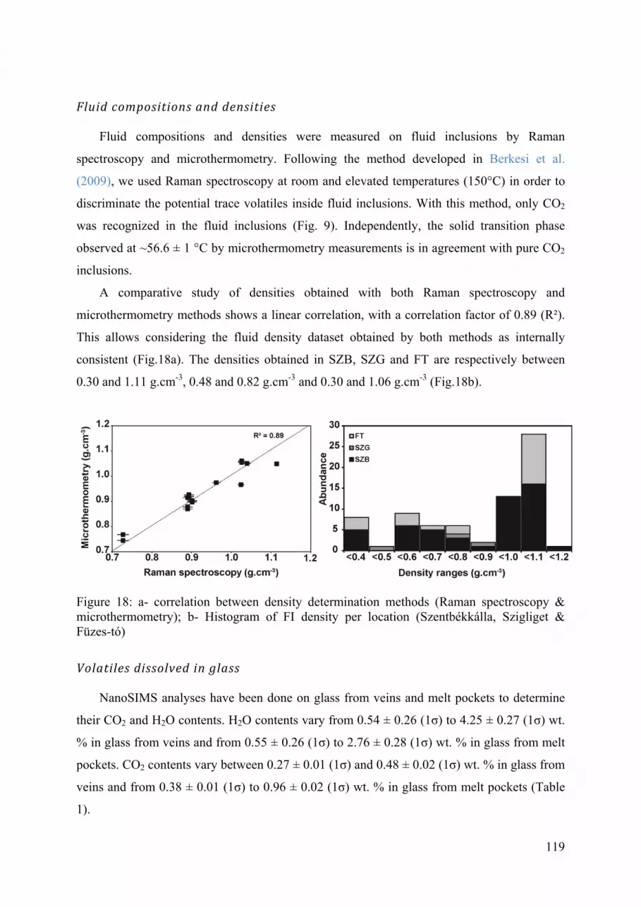
119

Fluidcompositionsand densities

Fluid compositions and densities were measured on fluid inclusions by Raman

spectroscopy and microthermometry. Following the method developed in Berkesi et al.

(2009), we used Raman spectroscopy at room and elevated temperatures (150°C) in order to

discriminate the potential trace volatiles inside fluid inclusions. With this method, only CO2

was recognized in the fluid inclusions (Fig. 9). Independently, the solid transition phase

observed at ~56.6 ± 1 °C by microthermometry measurements is in agreement with pure CO2

inclusions.

A comparative study of densities obtained with both Raman spectroscopy and

microthermometry methods shows a linear correlation, with a correlation factor of 0.89 (R²).

This allows considering the fluid density dataset obtained by both methods as internally

consistent (Fig.18a). The densities obtained in SZB, SZG and FT are respectively between

0.30 and 1.11 g.cm-3, 0.48 and 0.82 g.cm-3 and 0.30 and 1.06 g.cm-3 (Fig.18b).

Figure 18: a- correlation between density determination methods (Raman spectroscopy & microthermometry); b- Histogram of FI density per location (Szentbékkálla, Szigliget & Füzes-tó)

Volatilesdissolvedinglass

NanoSIMS analyses have been done on glass from veins and melt pockets to determine

their CO2 and H2O contents. H2O contents vary from 0.54 ± 0.26 (1σ) to 4.25 ± 0.27 (1σ) wt.

% in glass from veins and from 0.55 ± 0.26 (1σ) to 2.76 ± 0.28 (1σ) wt. % in glass from melt

pockets. CO2 contents vary between 0.27 ± 0.01 (1σ) and 0.48 ± 0.02 (1σ) wt. % in glass from

veins and from 0.38 ± 0.01 (1σ) to 0.96 ± 0.02 (1σ) wt. % in glass from melt pockets (Table

1).

120

        

  

  Vol. (cm3)  Glass volume (cm3)  Fluid volume (cm3)  Density (g/cm3)  Mass (g)     

Sample  MP  SiO2   H2O  Error (1σ)  CO2  

Error (1σ)  Minerals Best 

estimate Min (%)  Max (%) Best estimate Min (%)  Max (%) Glass  Vesicles  FI (Max) Glass  CO2 

(vesicle)CO2 

(dissolved)CO2/glass (wt. %) 

CO2/π (ppm) 

SZB16  no  56.6  0.54  0.26  0.29  0.14  4.6E‐03  9.1E‐05  3.7E+01  1.3E+01  5.5E‐05  1.5E+01  3.3E+01  2.599  1.022  0.573  2.4E‐04  5.6E‐05  6.8E‐07  24.1  3723 

SZB50  no  55.4  0.59  0.26  0.39  0.14  3.1E‐02  6.4E‐03  6.6E+00  6.4E+00  1.6E‐03  1.3E+00  1.4E+01  2.740  1.295  0.617  1.8E‐02  2.1E‐03  6.8E‐05  12.2  21287 

SZB51‐v  no  61.9  3.1  0.26  0.33  0.16 

6.0E‐03  2.1E‐04  1.4E+01  2.6E‐04  1.1E‐04  3.2E+01  2.0E+01  2.496  0.970  1.024  5.3E‐04  1.0E‐04  2.1E‐06  19.9  5409 SZB51‐MP  yes  56.6  2.76  0.28  0.46  0.15 

SZB51‐Av  yes  59.6  2.95  0.28  0.39  0.16 

SZB52  no  57.9  2.35  0.26  0.34  0.15  2.3E‐02  7.8E‐04  1.3E+01  1.0E‐03  3.4E‐04  5.8E+00  3.4E+01  2.452  0.953  1.114  1.9E‐03  3.3E‐04  6.5E‐06  17.4  4422 

SZG23  yes  56.3  2.38  0.26  0.96  0.20  3.5E‐02  6.1E‐03  2.3E+00  1.6E‐03  2.0E‐03  3.2E+00  1.3E+01  2.744  1.330  0.703  1.7E‐02  2.6E‐03  1.6E‐04  16.5  24383 

SZG44  yes  51.7  3.45  0.24  0.53  0.14  nd  

0.0E+00  0.0E+00  1.3E‐04  nd  nd  0.000  1.045  0.824  nd  1.4E‐04  nd  nd  nd 

FT12  yes  54.8  0.55  0.26  0.38  0.14  3.1E‐02  7.8E‐04  4.2E+00  9.7E‐04  4.0E‐04  1.0E+01  1.5E+01  2.542  1.228  0.661  2.0E‐03  5.0E‐04  7.5E‐06  25.4  4946 

FT01P  no  57.8  4.25  0.27  0.48  0.16  3.6E‐02  1.4E‐03  9.3E+00  1.7E‐03  3.3E‐04  4.9E+01  3.9E+01  2.611  0.930  1.057  3.6E‐03  3.0E‐04  1.7E‐05  9.0  2727 

Table 1: Summary table for petrographic observations, chemical compositions and phase volumes, densities and masses. V – vein; MP – melt pocket; Av – average composition; Vol. – volume; Min & Max – Relative determined errors for each best estimate; vs - vesicle; FI – fluid inclusion; gl – glass; π - peridotite

121

3.1.5 Discussion

Magma CO2-supersaturation conditions

Several petrographic evidences point to magma CO2-supersaturation at lithospheric

depths. Such evidences are 1) CO2 FI with densities above 1.0 g.cm-3 (Table 1),

corresponding to the lithospheric mantle below the present Moho depth (30 km, Kovacs et al.,

2012), 2) coexistence of melt + vesicle veins with high dissolved CO2 and H2O melt

concentrations of up to 0.96 and 4.25 wt. %, respectively (Table 1). In order to assess the

conditions of magma supersaturation, CO2 saturation isotherms have been calculated from the

different magma compositions determined by Creon et al. (in prep.) in the same samples and

for different temperatures using the Rhyolite-MELTS software (Gualda et al. 2012; Ghiorso

& Gualda 2015). The model is suited for calculation of thermodynamic equilibrium of mafic

to felsic systems with H2O and CO2 over the pressure range 0-3 GPa (Gualda et al. 2012;

Ghiorso & Gualda 2015) corresponding to the conditions of the lithospheric mantle below the

BBHVF (Kovacs et al. 2012).

Magma CO2-saturation show little temperature dependence between 1100 and 1300 °C

and for pressure below 0.5 GPa, as already shown by Shishkina et al. (2010) and

Botcharnikov et al. (2006). The effect of temperature tends to increase the solubility of CO2 in

the high pressure range of 0.5-3.0 GPa as also mentioned by Papale et al. (2006).

Based on CO2-saturation isotherms, vesicle-melt equilibrium pressures were assigned

from the CO2 contents of melts determined by NanoSIMS (Table 1, Figure 19). These

saturation pressures at 1100°C (corresponding to mineral equilibrium temperatures

determined in Creon et al., in prep.) are between 0.69 and 1.78 GPa and correspond to depths

of 26 to 62 km. Such estimations likely correspond to vesicle-melt equilibrium near the

attainment of the glass transition.

122

Figure 19: CO2 saturation curves draw with rhyolite-MELTS (Gualda et al. 2012; Ghiorso & Gualda 2015) using glass compositions obtained by EMPA and H2O contents obtained by nano-SIMS measurements. Saturation pressure estimations are obtained using CO2 contents in glass (NanoSIMS data) and CO2 saturation curves (grey lines). Black (SZB), dark-grey (SZG) and light-grey (FT) diamonds are crossing points between saturation curves and CO2 contents measured in glass by NanoSIMS experiments. The crossing points give the saturation pressure for each sample depending on its CO2 contents.

Glass transition temperatures (Tg) were constrained between 670 to 854°C by Giordano

et al. (2008), at asthenosphere pressures, and from 520 to 930°C by Morizet et al. (2007) at

pressures between 1 and 2.5 GPa (phonolite melts). CO2 appears to have almost no effect on

the glass transition of silicate melts unlike H2O, which reduces glass transition temperatures

(Morizet et al. 2007). Furthermore, pressures have very low influence on glass transition as

demonstrated by Bagdassarov et al. (2004). Such glass transition temperatures correspond to

pressures of ~0.54 Gpa using the geotherm of Kovacs et al. (2012), which are reached at

crustal levels (~20 km depth). Because melt pockets were shown to have crystallized at

lithospheric mantle pressures in co-existence with fluid vesicles (Creon et al., in prep.), the

crustal saturation pressures recorded for the most CO2 depleted melts is likely to reflect the

fast ascent of xenoliths after their extended residence time at lithospheric mantle depths.

Melt saturation pressures of 0.69 to 1.78 GPa have been converted in CO2 density using

the equations of states of Span & Wagner (1996) and Sterner & Pitzer (1994). The densities

123

obtained are between 0.93 and 1.33 g.cm-3, corresponding to the density range determined by

Raman and microthermometry recorded by the denser FIs (Table 1). This correspondence

attests to a coeval formation of FI and vesicles in lithospheric mantle conditions. However, no

direct correlation is observed between maximum fluid inclusion and vesicle densities, which

likely points to the instable behavior of FIs (Roedder 1984). In most cases (SZB16, SZB50,

SZG23, SZG44, FT12), fluid inclusion densities are lower than the associated calculated

vesicle densities; which can be related to decrepitation of the FIs during xenolith ascent

(Bodnar 2003). In other cases (SZB51, SZB52, FT01P) the densities of the fluid inclusions

are higher than those of the associated vesicles, as preserved fluid inclusion were trapped in

equilibrium with vesicles at pre-ascent lithospheric mantle pressures.

Figure 20: Density comparison for vesicles and FI. Vesicle densities are mostly higher than fluid inclusions within each sample.

CO2 contents dissolved in glass and measured by NanoSIMS (0.27-0.96 wt. %) are in

excess of those characteristic of arc magmas and within the E-MORB range following the

data compilation of Wallace (2005) (Fig. 21). Moreover, the CO2 and H2O contents measured

in this study are higher than those described in the literature in silicate melt pockets of the

BBHVF (Bali et al. 2002). Hidas et al. (2010) used SMI from Szigliget mantle xenoliths to

estimate the volatile content of trapped magmas. Calculated melt CO2 ~1 wt. % (Hidas et al.

2010) are in agreement with the maximum CO2 content measured in glass for this study in

sample SZG23 (Fig. 21). It is thus likely that silicate melt inclusions (SMI) in Hidas et al.

124

(2010) correspond to the trapping of a melt similar to the CO2-richest percolating melts

analyzed in this study, during the growth of clinopyroxenes in the mantle lithosphere.

CO2 contents in lithospheric melts

3D images have illustrated an interconnection between trails of secondary fluid

inclusions and the glass + vesicles network. This observation is in contradiction with the

observations of Demény et al. (2010) on similar samples from the same sample localities, who

reported the lack of extension of FI trails to grain boundaries from thin section examinations.

We strongly favor our observation, as the 3D reconstructions show clear crosscutting

relationships of FI trails with grain boundaries. These observations are petrographic evidences

of a co-genetic relationship between FI and melt percolation in mantle xenoliths. With the

impossibility to investigate fluid compositions and densities of vesicles because of their too

large dimensions for any preservation after thin section and plug preparation, we assumed that

vesicles have similar compositions to FIs. Vesicles are therefore interpreted to be mainly

composed of CO2. This assumption is confirmed by the volatile contents in glass determined

by nanoSIMS, which imply the supersaturation of the melt with a pure CO2 phase

corresponding to the abundant vesicles observed.

The CO2/glass mass ratio corresponding to the melt + vesicle system has been calculated

using equation (1):

1 2 2 ∗ρ CO2

V(CO2), V(glass) and ρ(glass) are obtained by synchrotron X-ray microtomography and

ρ(CO2) was obtained by NanoSIMS analyses and thermodynamical modeling (Rhyolite-

MELTS, Gualda et al. 2012; Ghiorso & Gualda 2015) as described in the previous section.

The CO2/melt mass ratios obtained are comprised between 9.0 and 25.4 wt. % (Table 1).

These ratios, which can be considered as the CO2 mass fraction of the melt system, would

correspond to a single phase system at pressures of 4 to 9 Gpa following Guillot & Sator

(2011) for basaltic melts. The present lithosphere-asthenosphere boundary below the

Pannonian basin is estimated at depths between 60 and 100 km (Tašárová et al. 2009). The

melts characterized here were therefore likely supersaturated in the asthenosphere prior to

reaching lithospheric depth.

125

The range of CO2/melt mass ratios calculated in this study implies a varying proportion

of CO2 in melts either due to magmatic processes or to physical fractionation. Here, we

review the various processes that might affect the CO2/melt ratio in lithospheric melts.

Figure 21: H2O vs. CO2 for glass trapped as vein or melt pockets in mantle xenoliths. Shown for comparisons melt inclusions from arc basalts (Modified from Wallace, 2005). Literature data are shown for Cerro Negro (Roggensack 1997), Fuego (Fg; Roggensack 2001), Guatemalan volcanoes behind the volcanic front (Guat BVF; Walker et al. 2003), the Trans-Mexican Volcanic Belt (Luhr 2001; Cervantes & Wallace 2003), Stromboli (Metrich et al. 2001) and Cayuse Crater, a cinder cone with OIB-like trace element composition from the Oregon Cascades (Cas OIB; M. Rowe, unpublished data). For Cerro Negro, only inclusions from the 1992 explosive eruption are plotted. Shown for information are the primary CO2 contents of N-MORB (Marty & Tolstikhin 1998), E-MORB (Hekinian et al. 2000) magmas, Kilauea basaltic magma (Gerlach et al. 2002) and popping-rock (Graham & Sarda 1991). Also shown is the CO2 content of basaltic magma from Reunion based on rare high-pressure melt inclusions (Bureau et al. 1999).

126

Magmatic Sources of CO2 and CO2/melt physical fractionation

Carbonate minerals have been described in the Pannonian xenoliths from the BBHVF.

These carbonate phases are mainly calcitic droplets (Demény et al. 2004), rounded (Bali et al.

2002; 2008) or anhedral (Chalot-Prat & Arnold 1999) crystals in silicate veins and/or melt

pockets of mantle xenoliths. Bali et al. (2002) and Demény et al. (2004) argued for the

infiltration of a mixed carbonate–silicate melt in those mantle xenoliths, which support our

observations. These arguments confirm that carbonates are not the source of the melts, but

are due to carbon saturation and immiscibility in the percolating silicate melts.

Creon et al. (in prep.) interpreted the percolating melts studied here as adakite-like

magmas, derived from slab melting. Wallace (2005) compiled CO2 contents of silicate melt

inclusions from arc-magmas worldwide that cluster between 0-2100 ppm. These

concentrations are much lower than the values determined in this study. We suggest here that

arc magmas sampled by SMIs represent a negligible fraction of the CO2 associated with slab-

derived melts. Similarly, as for samples of the BBHVF analyzed by Bali et al. (2008) and

Hidas et al. (2010), only a very small fraction of the melt CO2 may be trapped as SMIs

because of pre-entrapment supersaturation of the melt, and accumulation of the larger

proportion of the CO2 (95-98 % in our samples) in vesicles and FIs rather than in the silicate

melt. Consequently, melt inclusions only rarely melts trapped with their primary CO2 contents

(e.g., Saal et al. 2002). This assumption conforms with the work of Watson & Brenan (1987)

who showed that CO2 has a very low tendency to wet grain edges contrary to water and melts,

as we observe in our samples (Fig.3c, g, h). This implies a very low probability for crystals

growing from grain boundary melt to trap vesicle gas. Contrarily, grain fractionation due to

mantle creep or to overpressure may much more easily trap vesicle volatiles due their

preferential viscosity-controlled injection in such a fast crack-and-seal process (Watson and

Brenan, 1987). We suspect here that a large physical fractionation of CO2 from silicate melts

is to be expected due to the formation of fluid inclusion in minerals along the migration path

of the percolating melt + vesicle system. The volume correlation observed for melt and fluid

seems therefore to reflect the degassing of a melt in a closed system and of the conservative

percolation of a diphasic system of melt + volatile. The widespread FI formation process

occurring in the lithospheric mantle, and potentially below, may explain much of the

variations in the CO2/melt mass ratios.

Figure 22 illustrates the H2O and CO2 sources expected in a subduction context where 1)

E-MORB, 2) altered oceanic basalts and 3) subducted sediments (Plank & Langmuir 1998;

127

Staudigel et al. 1989; Wallace 2005) represent end-members of slab melting. Partial melting

of the slab, and/or of the metasomatized mantle wedge, would induce incompatible element-

rich melts with high CO2 and H2O contents as those calculated in this study (0.55 to 4.25 wt.

% H2O and 9.0 to 25.4 wt. % CO2). Dasgupta et al. (2013) experimentally showed that

carbonated silicate melt with 15-25 wt. % CO2 and modest amount of water (1-5 wt. %) can

be generated in the upper part of the asthenospheric mantle (1,300-1,750 °C and 2-5 GPa) and

percolate to the lithospheric mantle. The high carbonation of peridotite may easily be

produced in the mantle wedge due to massive degassing of carbonates from the slab (Frezzotti

et al., 2009; Ague & Nicolescu, 2014).

We conclude that the CO2/melt ratios determined in this study correspond to deep melts

derived from slab melting, which have percolated to lithospheric depths without having

substantially fractionated.

A lithospheric carbon reservoir?

The mass ratio of CO2/peridotite have been calculated for each sample, giving values

between 2700 and 24,400 ppm with an average of about 9557 ppm, which is considered

representative of the average quantity of carbon stored in the samples examined. However, the

present study is based on fluid inclusion rich samples only, which correspond to ~20 % of an

initial sample set of mantle xenoliths. Considering that the non-studied 80% of the initial

sample set contains in average 30 ppm carbon, as estimated for the N-MORB mantle (Marty

2012), a first estimation of the CO2 content present in the Pannonian lithospheric mantle can

be made. We define a first order value of 0.2 x 9557 ppm + 0.8 x 30 ppm = 1935 ppm CO2.

This value can be considered as representative of the bulk lithospheric mantle sampled by

alkaline volcanism of the BBHVF. This estimation is on the same order of magnitude as the

1000 ppm estimated by Kelemen & Manning (2015) for the back-arc lithospheric mantle

based on observed carbon fluxes and reservoirs at subduction zones. For comparison, the

carbon content at source regions of MORB is comprised approximately between 50 and 200

ppm, and between 1000 and 4000 ppm in the source mantle of OIB (Saal et al. 2002; Cartigny

et al. 2008; Marty & Tolstikhin 1998; Pineau et al. 2004). We suggest that the quantitative

peridotite + melt + volatile features described here, and found in many other regions of the

Earth, may be representative of the carbon stock in the lithospheric mantle.

128

Figure 22: H2O-CO2 diagram illustrating nanoSIMS H2O/CO2 data measured in peridotite melts, and reconstructed CO2 contents of slab derived parental melts. Slab derived parental melts are obtained by partial melting of a subducted lithosphere; Pannonian lithosphere melts correspond to the low undegassed part of the slab derived melts.

Besides the implications of our findings for the carbon cycle, such a lithospheric carbon

reservoir has several consequences for the degassing of mantle volatiles in active geodynamic

contexts, such as the one characterizing the PB. Mantle-derived CO2 occurrences in the

Pannonian sedimentary basin may be one of these consequences. This suggests that the

carbon reservoir of ~2000 ppm quantified in this study in only transient, and may be recycled

to the atmosphere and to the asthenosphere over geodynamic timescales by passive tectonic

degassing and delamination, respectively.

129

3.1.6 Conclusions

The magmatic-CO2 budget of the mantle below the Pannonian Basin has been

constrained by an innovating approach using the coupling of: (1) synchrotron 3D X-ray

microtomography, (2) nanoSIMS, Raman spectroscopy and microthermometry experiments

and (3) thermodynamical modeling to investigate the significance of abundant CO2 inclusions

and vesicles within lithospheric peridotites.

3D volume reconstructions have illustrated an interconnection between trails of

secondary fluid inclusions and the glass + vesicles network, describing a co-genetic

relationship between FI and melt percolation in mantle xenoliths. The volatile phase (vesicles

+ FI) presence also highlights the CO2-supersaturation of the silicate melts.

The CO2/glass mass ratio corresponding to the melt + vesicle system has been calculated

using VCO2 (0.7-4.7 vol. %), Vglass (0-23.4 vol. %) and ρglass (2.45-2.74 g.cm-3) obtained by

synchrotron X-ray microtomography and ρCO2 (0.30-1.11 g.cm-3) obtained by NanoSIMS

analyses and thermodynamical modeling (rhyolite-MELTS, Gualda et al. 2012; Ghiorso &

Gualda 2015). The CO2/melt mass ratios obtained are comprised between 9.0 and 25.4 wt. %,

and are related to a slab-derived melting source. A first estimation of CO2 content present in

the Pannonian lithospheric mantle is proposed at ~2000 ppm and can be considered as

representative of the bulk lithospheric mantle sampled by the alkaline volcanism of the

BBHVF.

This petro-geochemical approach is in agreement with independent assumptions made on

the lithospheric carbon stock based on carbon fluxes in subduction-arc systems, and requires

to be applied in other contexts to bring our results to more systematic evidence.

3.1.7 References

Adam, J. (1990). The geochemistry and experimental petrology of sodic alkaline basalts from Oatlands, Tasmania. Journal of Petrology, 31(6), 1201–1223. http://doi.org/10.1093/petrology/31.6.1201

Ague, J. J., & Nicolescu, S. (2014). Carbon dioxide released from subduction zones by fluid-mediated reactions. Nature Geoscience, 7(5), 2–7. http://doi.org/10.1038/NGEO2143

Alt, J. C., Schwarzenbach, E. M., Früh-Green, G. L., Shanks, W. C., Bernasconi, S. M., Garrido, C. J., … Marchesi, C. (2013). The role of serpentinites in cycling of carbon and sulfur: Seafloor serpentinization and subduction metamorphism. Lithos, 178, 40–54. http://doi.org/10.1016/j.lithos.2012.12.006

Anderson, a. T. (1975). Some basaltic and andesitic gases. Reviews of Geophysics, 13(1), 37.

130

http://doi.org/10.1029/RG013i001p00037

Babuška, V., PlomerovÁ, J., & Granet, M. (1990). The deep lithosphere in the Alps: a model inferred from P residuals. Tectonophysics, 176(1-2), 137–165. http://doi.org/10.1016/0040-1951(90)90263-8

Bagdassarov, N. S., Maumus, J., Poe, B., Slutskiy, A. B., & Bulatov, V. K. (2004). Pressure dependence of T g in silicate glasses from electrical impedance measurements. Physics and Chemistry of Glasses - European Journal of Glass Science and Technology Part B, 45(3), 197–214. Retrieved from http://www.ingentaconnect.com/content/sgt/pcg/2004/00000045/00000003/art00007

Bali, E., Szabo, C., Vaselli, O., Torok, K., & Bali, Eniko; Szabo, Csaba; Vaselli, Orlando; Szabo, C. (2002). Significance of silicate melt pockets in upper mantle xenoliths from the Bakony – Balaton Highland Volcanic Field , Western Hungary. Lithos, 61, 79–102.

Bali, E., Zajacs, Z., Kovacs, I., Szabo, C., Halter, W., Vaselli, O., … Bodnar, R. J. (2008). A Quartz-bearing Orthopyroxene-rich Websterite Xenolith from the Pannonian Basin , Western Hungary : Evidence for Release of Quartz-saturated Melts from a Subducted Slab. Journal of Petrology, 49(3), 421–439. http://doi.org/10.1093/petrology/egm086

Bali, E., Zanetti, A., Szabó, C., Peate, D. W., & Waight, T. E. (2008). A micro-scale investigation of melt production and extraction in the upper mantle based on silicate melt pockets in ultramafic xenoliths from the Bakony–Balaton Highland Volcanic Field (Western Hungary). Contributions to Mineralogy and Petrology, 155(2), 165–179. http://doi.org/10.1007/s00410-007-0234-4

Ballentine, C. J., O’Nions, R. K., Oxburgh, E. R., Horvath, F., & Deak, J. (1991). Rare gas constraints on hydrocarbon accumulation, crustal degassing and groundwater flow in the Pannonian Basin. Earth and Planetary Science Letters, 105(1-3), 229–246. http://doi.org/10.1016/0012-821X(91)90133-3

Ballentine, C. J., Schoell, M., Coleman, D., & Cain, B. a. (2001). 300-Myr-old magmatic CO2 in natural gas reservoirs of the west Texas Permian basin. Nature, 409(6818), 327–31. http://doi.org/10.1038/35053046

Balogh, K., Jambor, A., Partenyi, Z., Ravaszné Baranyai, L., & Solti, G. (1982). A dunantuli bazaltok K/Ar radiometrikus kora. M. All. Foldt. Int. Jel, 243–260.

Balogh, K., & Németh, K. (2005). Evidence for the Neogene small-volume intracontinental volcanism in Western Hungary: K/Ar geochronology of the Tihany Maar Volcanic Complex. Geologica Carpathica, 56, 91–99.

Balogh, K., & Pécskay, Z. (2001). K/Ar and Ar/Ar geochronological studies in the Pannonian-Carpathians-Dinarides (PANCARDI) region. Acta Geol. Hung., 44, 281–299.

Bartoli, O., Cesare, B., Remusat, L., Acosta-Vigil, A., & Poli, S. (2014). The H2O content of granite embryos. Earth and Planetary Science Letters, 395, 281–290. http://doi.org/10.1016/j.epsl.2014.03.031

Baruchel, J., Buffiere, J.-Y., Maire, E., Merle, P., & Peix, G. (2000). X-ray Tomography in Material Science. Hermes Science Publications.

Berkesi, M., Hidas, K., Guzmics, T., Dubessy, J., Bodnar, R. J., Szabo, C., … Tsunogae, T. (2009). Detection of small amounts of H2O in CO2-rich fluid inclusions using Raman spectroscopy. Journal of Raman Spectroscopy, 40(11), 1461–1463. http://doi.org/10.1002/jrs.2440

131

Bodnar, R. J. (2003). Re-equilibration of fluid inclusions. In: Fluid Inclusions: Analysis and Interpretation, Short Course Series. Samson I, Anderson A, Marshall D (eds) Mineral Assoc Can, Vancouver, 32, 213–231.

Bonelli, R., & Frezzotti, M. . (2003). Raman Spectra Database. http://www.dst.unisi.it/geofluidslab/Raman%20intro.html.

Borsy, Z., Balogh, K., Kozak, M., & Pécskay, Z. (1986). Újabb adatok a Tapolcai-medence fejlõdéstörténetéhez (Con-tributions to the evolution of the Tapolca-basin, Hungary). Acta Geographica Debre-Cina, 23, 79–104.

Botcharnikov, R., Behrens, H., & Holtz, F. (2006). Solubility and speciation of C–O–H fluids in andesitic melt at T=1100–1300°C and P=200 and 500MPa. Chemical Geology, 229(1-3), 125–143. http://doi.org/10.1016/j.chemgeo.2006.01.016

Bruce Watson, E., & Brenan, J. M. (1987). Fluids in the lithosphere, 1. Experimentally-determined wetting characteristics of CO2H2O fluids and their implications for fluid transport, host-rock physical properties, and fluid inclusion formation. Earth and Planetary Science Letters, 85(4), 497–515. http://doi.org/10.1016/0012-821X(87)90144-0

Bureau, H., Métrich, N., Semet, M. P., & Staudacher, T. (1999). Fluid magma decoupling in a hotspot volcano. Geophysical Research Letters, 26(23), 3501. http://doi.org/10.1029/1999GL005422

Burton, M. R., Sawyer, G. M., & Granieri, D. (2013). Deep Carbon Emissions from Volcanoes. Review in Mineralogy and Geochemistry, 75(1), 323–354. http://doi.org/10.2138/rmg.2013.75.11

Cartigny, P., Pineau, F., Aubaud, C., & Javoy, M. (2008). Towards a consistent mantle carbon flux estimate: Insights from volatile systematics (H2O/Ce, δD, CO2/Nb) in the North Atlantic mantle (14° N and 34° N). Earth and Planetary Science Letters, 265(3-4), 672–685. http://doi.org/10.1016/j.epsl.2007.11.011

Cervantes, P., & Wallace, P. (2003). Magma degassing and basaltic eruption styles: A case study of ~2000 year BP Xitle volcano in central Mexico. Journal of Volcanology and Geothermal Research, 120(3-4), 249–270. http://doi.org/10.1016/S0377-0273(02)00401-8

Chalot-Prat, F., & Arnold, M. (1999). Immiscibility between calciocarbonatitic and silicate melts and related wall rock reactions in the upper mantle: a natural case study from Romanian mantle xenoliths. Lithos, 46, 627–659.

Creon, L., Delpech, G., Rouchon, V., Guyot, F., & Szabo, C. (n.d.). Melt-peridotite interaction in the lithospheric mantle - Genesis of the Pannonian calc-alkaline suites revealed by Alkali basalt hosted xenoliths. Geochemica et Cosmochimica Acta.

Csontos, L., Nagymarosy, A., Horváth, F., & Kovác, M. (1992). Tertiary evolution of the Intra-Carpathian area: a model. Teconophysics, 208, 221–241.

Dasgupta, R. (2013). Ingassing, Storage, and Outgassing of Terrestrial Carbon through Geologic Time. Reviews in Mineralogy and Geochemistry, 75, 183–229. http://doi.org/10.2138/rmg.2013.75.7

Dasgupta, R., & Hirschmann, M. M. (2010). The deep carbon cycle and melting in Earth’s interior. Earth and Planetary Science Letters, 298(1-2), 1–13. http://doi.org/10.1016/j.epsl.2010.06.039

132

Dasgupta, R., Mallik, A., Tsuno, K., Withers, A. C., Hirth, G., & Hirschmann, M. M. (2013). Carbon-dioxide-rich silicate melt in the Earth’s upper mantle. Nature, 493(7431), 211–215. http://doi.org/10.1038/nature11731

Demény, A., Dallai, L., Frezzotti, M.-L., Vennemann, T. W., Embey-Isztin, A., Dobosi, G., & Nagy, G. (2010). Origin of CO2 and carbonate veins in mantle-derived xenoliths in the Pannonian Basin. Lithos, 117(1-4), 172–182. http://doi.org/10.1016/j.lithos.2010.02.013

Demény, A., Vennemann, T. ., Hegner, E., Nagy, G., Milton, J. ., Embey-Isztin, A., … Dobosi, G. (2004). Trace element and C–O–Sr–Nd isotope evidence for subduction-related carbonate–silicate melts in mantle xenoliths (Pannonian Basin, Hungary). Lithos, 75(1-2), 89–113. http://doi.org/10.1016/j.lithos.2003.12.016

Dixon, J. E., Stolper, E. M., & Holloway, J. R. (1995). An Experimental Study of Water and Carbon Dioxide Solubilities in Mid-Ocean Ridge Basaltic Liquids . Part I : Calibration and Solubility Models. Journal of Petrology, 36(6), 1607–1631.

Dovenyi, P., & Horvath, F. (1988). A review of temperature, thermal conductivity, and heat flow data for the Pannonian Basin. American Association of Petroleum Geologists, 45, 195–233.

Downes, H., Embey-Isztin, A., & Thirlwall, M. F. F. . (1992). Petrology and geochemistry of spinel peridotite xenoliths from the western Pannonian Basin (Hungary): evidence for an association between enrichment and texture in the upper mantle. Contribution of Mineralogy and Petrology, 109, 340–354.

Downes, H., & Vaselli, O. (1995). The lithospheric mantle beneath the Carpathian-Pannonian Region: a review of trace element and isotopic evidence from ultramafic xenoliths. In: Downes H. & Vaselli O. (Eds.): Neogene and related magmatism in the Carpatho-Pannonian Region. ACta Vulcanologica, 7, 219–229.

Dunn, P. K. (2007). tweedie: Tweedie exponential family models.

Embey-Isztin, a, Dobosi, G., Altherr, R., & Meyer, H.-P. (2001). Thermal evolution of the lithosphere beneath the western Pannonian Basin: evidence from deep-seated xenoliths. Tectonophysics, 331(3), 285–306. http://doi.org/10.1016/S0040-1951(00)00287-0

Embey-Isztin, A. (1976). Amphibolite/lherzolite composite xenolith from Szigliget, north of the Lake Balaton, Hungary. Earth and Planetary Science Letters, 31, 297–304.

Embey-isztin, A., Downes, H., James, D. E. E., Upton, B. G. J. G. J., Dobosi, G., Ingram, G. A. a., … Scharbert, H. G. G. (1993). The petrogenesis of Pliocene alkaline volcanic rocks from the Pannonian Basin, Eastern central Europe. Journal of Petrology, 34, 317–343. http://doi.org/10.1093/petrology/34.2.317

Embey-Isztin, A., Scharbert, H. G., Dietrich, H., & Poultidis, H. (1989). Petrology and geochemistry of peridotite xenoliths in alkali basalts from the Transdanubian volcanic region. Journal of Petrology, 30(1), 79–106.

Embey-Isztin, A., Sharbert, H. G., Dietrich, H., & Poultidis, H. (1990). Mafic granulites and clinopyroxenite xenoliths from the Transda- nubian Volcanic Region (Hungary): implications for the deep structure of the Pannonian Basin. Mineralogica Magazine, 54, 463–483.

Fall, A., Tattitch, B., & Bodnar, R. J. (2011). Combined microthermometric and Raman spectroscopic technique to determine the salinity of H2O–CO2–NaCl fluid inclusions based on clathrate melting. Geochimica et Cosmochimica Acta, 75(4), 951–964.

133

http://doi.org/10.1016/j.gca.2010.11.021

Falus, G., Drury, M. R., van Roermund, H. L. M., & Szabo, C. (2004). Magmatism-related localized deformation in the mantle: a case study. Contributions to Mineralogy and Petrology, 146(4), 493–505. http://doi.org/10.1007/s00410-003-0513-7

Falus, G., Szabó, C., Kovács, I., Zajacz, Z., & Halter, W. (2007). Symplectite in spinel lherzolite xenoliths from the Little Hungarian Plain, Western Hungary: A key for understanding the complex history of the upper mantle of the Pannonian Basin. Lithos, 94(1-4), 230–247. http://doi.org/10.1016/j.lithos.2006.06.017

Fleet, A. J., Wycherley, H., & Shaw, H. (1998). Large Volume of carbon dioxide in sedimentary basins. Mineralogica Magazine, 62A, 460–461.

Fodor, L., Csontos, L., Bada, G., Györfi, I., & Benkovics, L. (1999). Tertiary tectonic evolution of the Pannonian basin and neighbouring orogenes: a new synthesis of palaeostress data. In: Durand, B., Jolivet, L., Horváth, F., Séranne, M. (Eds.), The Mediterranean Basins: Tertiary Extension with Alpine Orogen. Geological Society, 156(Special Publication, London), 295–334.

Frezzotti, M. L., Peccerillo, A., Panza, G., Frezzotti, Peccerillo, & Panza. (2009). Carbonate metasomatism and CO2 lithosphere–asthenosphere degassing beneath the Western Mediterranean: An integrated model arising from petrological and geophysical data. Chemical Geology, 262(1-2), 108–120. http://doi.org/10.1016/j.chemgeo.2009.02.015

Fyfe, W. S., Price, N. J., & Hompson, A. B. (1978). Fluids in the Earth’s Crust: Their Significance in Metamorphic, Tectonic, and Chemical Transport Processes. Elsevier, Amsterdam, 384 pp.

Gerlach, T. M., McGee, K. A., Elias, T., Sutton, A. J., & Doukas, M. P. (2002). Carbon dioxide emission rate of Kilauea volcano: implications for primary magma and the summit reservoir. Journal of Geophysical Research, 107, 2189–2203.

Ghiorso, M. S., & Gualda, G. A. R. (2015). An H2O-CO2 mixed fluid saturation model compatible with rhyolite-MELTS. Contributions to Mineralogy and Petrology.

Giordano, D., Russell, J. K., & Dingwell, D. B. (2008). Viscosity of magmatic liquids: A model. Earth and Planetary Science Letters, 271(1-4), 123–134. http://doi.org/10.1016/j.epsl.2008.03.038

Gorman, P. J., Kerrick, D. M., & Connolly, J. a D. (2006). Modeling open system metamorphic decarbonation of subducting slabs. Geochemistry, Geophysics, Geosystems, 7(4). http://doi.org/10.1029/2005GC001125

Graham, D., & Sarda, P. (1991). Reply to comment by T . M . Gerlach on “ Mid-ocean ridge popping rocks : implications for degassing at ridge crests .” Earth and Planetary Science Letters, 105, 568–573. http://doi.org/10.1016/0012-821X(91)90194-M

Gualda, G.A.R. et al., 2012. Rhyolite-MELTS: a Modified Calibration of MELTS Optimized for Silica-rich, Fluid-bearing Magmatic Systems. Journal of Petrology, 53(5), pp.875–890.

Guillot, B., & Sator, N. (2011). Carbon dioxide in silicate melts: A molecular dynamics simulation study. Geochimica et Cosmochimica Acta, 75(7), 1829–1857. http://doi.org/10.1016/j.gca.2011.01.004

Hammouda, T. (2003). High-pressure melting of carbonated eclogite and experimental constraints on carbon recycling and storage in the mantle. Earth and Planetary Science

134

Letters, 214(1-2), 357–368. http://doi.org/10.1016/S0012-821X(03)00361-3

Harangi, S., & Lenkey, L. (2007). Genesis of the Neogene to Quaternary volcanism in the Carpatian Pannonian region : Role of subduction , extension , and mantle plume. Geological Society of America, Special Pa, 67–92. http://doi.org/10.1130/2007.2418(04).

Hekinian, R., Pineau, F., Shilobreeva, S., Bideau, D., Gracia, E., & Javoy, M. (2000). Deep sea explosive activity on the Mid-Atlantic Ridge near 34 degrees 50 ’ N: Magma composition, vesicularity and volatile content. Journal of Volcanology and Geothermal Research, 98(1-4), 49–77. http://doi.org/10.1016/S0377-0273(99)00190-0

Hidas, K., Guzmics, T., Szabó, C., Kovács, I., Bodnar, R. J., Zajacz, Z., … Perucchi, A. (2010). Coexisting silicate melt inclusions and H2O-bearing, CO2-rich fluid inclusions in mantle peridotite xenoliths from the Carpathian–Pannonian region (central Hungary). Chemical Geology, 274(1-2), 1–18. http://doi.org/10.1016/j.chemgeo.2010.03.004

Horvath, F. (1993). Towards a mechanical model for the formation of the Pannonian Basin. Tectonophysics, 226, 333–357.

Horváth, F., Musitz, B., Balázs, a., Végh, A., Uhrin, a., Nádor, A., … Wórum, G. (2015). Evolution of the Pannonian basin and its geothermal resources. Geothermics, 53, 328–352. http://doi.org/10.1016/j.geothermics.2014.07.009

Huismans, R. S., Podladchikov, Y. Y., & Cloetingh, S. a. P. L. (2002). The Pannonian basin: Dynamic modelling of the transition from passive to active rifting. In EGU Special publication Series (Vol. 3, pp. 41–63). http://doi.org/10.5194/smsps-3-41-2002

Imbus, S. W., Katz, B. J., & Urwongse, T. (1998). Predicting CO2 occurence on a regional scale : Southeast Asia example. Organic Geochemistry, 29(1-3), 325–345.

Jambon, A. (1994). Earth degassing and large-scale geochemical cycling of volatile elements. Volatiles in Magmas, 30, 479–517.

Jarrard, R. D. (2003). Subduction fluxes of water, carbon dioxide, chlorine, and potassium. Geochemistry, Geophysics, Geosystems, 4(5). http://doi.org/10.1029/2002GC000392

Johnston, F. K. B., Turchyn, A. V., & Edmonds, M. (2011). Decarbonation efficiency in subduction zones: Implications for warm Cretaceous climates. Earth and Planetary Science Letters, 303(1-2), 143–152. http://doi.org/10.1016/j.epsl.2010.12.049

Jugovics, L. (1969). A dunantuli bazalt es bazalttufa teruletek. In: Annual geological report of Hungary, 1967. MAFI, Budapest, 75–82.

Kazmer, M., & Kovacs, S. (1985). ermian–Paleogene paleogeography along the Eastern part of the Insubric–Periadriatic Lineament system: evidence for continental escape of the Bakony- Drauzug unit. Acta Geol. Hung., 1-2, 71–84.

Kelemen, P. B., & Manning, C. E. (2015). Reevaluating carbon fluxes in subduction zones, what goes down, mostly comes up. Proceedings of the National Academy of Sciences, 201507889. http://doi.org/10.1073/pnas.1507889112

Kovacs, I., Falus, G., Stuart, G., Hidas, K., Szabó, C., Flower, M. F. J., … Zilahi-Sebess, L. (2012). Seismic anisotropy and deformation patterns in upper mantle xenoliths from the central Carpathian–Pannonian region: Asthenospheric flow as a driving force for Cenozoic extension and extrusion? Tectonophysics, 514-517, 168–179. http://doi.org/10.1016/j.tecto.2011.10.022

135

Kovács, I., & Szabó, C. (2008). Middle Miocene volcanism in the vicinity of the Middle Hungarian zone: Evidence for an inherited enriched mantle source. Journal of Geodynamics, 45(1), 1–17. http://doi.org/10.1016/j.jog.2007.06.002

Luhr, J. F. (2001). Glass inclusions and melt volatile contents at Parícutin Volcano, Mexico. Contributions to Mineralogy and Petrology, 142(3), 261–283. http://doi.org/10.1007/s004100100293

Martin, U., Auer, A., Németh, K., & Breitkreuz, C. (2003). Mio-pliocene phreatomagmatic volcanism in a Fluvio–Lacustrine basin in Western Hungary. GeoLines, 15, 93–97.

Marty, B. (2012). The origins and concentrations of water, carbon, nitrogen and noble gases on Earth. Earth and Planetary Science Letters, 313-314(1), 56–66. http://doi.org/10.1016/j.epsl.2011.10.040

Marty, B., & Tolstikhin, I. N. (1998). CO2 fluxes from mid-ocean ridges, arcs and plumes. Chemical Geology, 145(3-4), 233–248. http://doi.org/10.1016/S0009-2541(97)00145-9

Mercier, J. C., & Nicolas, A. (1975). Textures and Fabrics of Upper-Mantle Peridotites as Illustrated by Xenoliths from Basalts. Journal of Petrology, 16(2).

Metrich, N., Bertagnini, a, Landi, P., & Rosi, M. (2001). Crystallization driven by decompression and water loss at Stromboli volcano (Aeolian Islands, Italy). Journal of Petrology, 42(8), 1471–1490. http://doi.org/10.1093/petrology/42.8.1471

Metrich, N. et al., 2014. Is the “Azores Hotspot” a Wetspot? Insights from the Geochemistry of Fluid and Melt Inclusions in Olivine of Pico Basalts. Journal of Petrology, 55(2), pp.377–393.

Morizet, Y., Nichols, A. R. L., Kohn, S. C., Brooker, R. a., & Dingwell, D. B. (2007). The influence of H2O and CO2 on the glass transition temperature: insights into the effects of volatiles on magma viscosity. European Journal of Mineralogy, 19(5), 657–669. http://doi.org/10.1127/0935-1221/2007/0019-1751

Papale, P., Moretti, R., & Barbato, D. (2006). The compositional dependence of the saturation surface of H2O+CO2 fluids in silicate melts. Chemical Geology, 229(1-3), 78–95. http://doi.org/10.1016/j.chemgeo.2006.01.013

Pineau, F., Shilobreeva, S., Hekinian, R., Bideau, D., & Javoy, M. (2004). Deep-sea explosive activity on the Mid-Atlantic Ridge near 34°50′N: a stable isotope (C, H, O) study. Chemical Geology, 211(1-2), 159–175. http://doi.org/10.1016/j.chemgeo.2004.06.029

Plank, T., & Langmuir, C. H. (1998). The chemical composition of subducting sediment and its consequences for the crust and mantle. Chemical Geology, 145(3-4), 325–394. http://doi.org/10.1016/S0009-2541(97)00150-2

Poinar, K. (2012). The Carbon Cycle in the Mantle.

Posgay, K., Albu, I., Petrovics, I., & Raner, G. (1981). Character of the Earth’s crust and upper mantle on the basis of seismic reflection measurements in Hungary. Earth Evol. Sci., 1 (3/4), 272–279.

Praus, O., Pěčová, J., Petr, V., Babuška, V., & Plomerová, J. (1990). Magnetotelluric and seismological determination of the lithosphere-asthenosphere transition in Central Europe. Physics of the Earth and Planetary Interiors, 60(1-4), 212–228. http://doi.org/10.1016/0031-9201(90)90262-V

Richet, P., Whittington, A., Holtz, F., Behrens, H., Ohlhorst, S., & Wilke, M. (2000). Water

136

and the density of silicate glasses. Contributions to Mineralogy and Petrology, 138(4), 337–347. http://doi.org/10.1007/s004100050567

Roedder, E. (1984). Fluid inclusions. Review in Mineralogy, 12.

Roggensack, K. (1997). Explosive Basaltic Volcanism from Cerro Negro Volcano: Influence of Volatiles on Eruptive Style. Science, 277(5332), 1639–1642. http://doi.org/10.1126/science.277.5332.1639

Roggensack, K. (2001). Sizing up crystals and their melt inclusions: A new approachto crystallization studies. Earth and Planetary Science Letters, 187, 221–237. http://doi.org/10.1016/S0012-821X(01)00269-2

Saal, A. E., Hauri, E. H., Langmuir, C. H., & Perfit, M. R. (2002). Vapour undersaturation in primitive mid-ocean-ridge basalt and the volatile content of Earth’s upper mantle. Nature, 419(6906), 451–5. http://doi.org/10.1038/nature01073

Sano, Y., & Marty, B. (1995). Origin of carbon in fumarolic gas from island arcs. Chemical Geology, 119(1-4), 265–274. http://doi.org/10.1016/0009-2541(94)00097-R

Shcheka, S. S., Wiedenbeck, M., Frost, D. J., & Keppler, H. (2006). Carbon solubility in mantle minerals. Earth and Planetary Science Letters, 245(3-4), 730–742. http://doi.org/10.1016/j.epsl.2006.03.036

Sherwood Lollar, B., Ballentine, C. J., & Onions, R. K. (1997). The fate of mantle-derived carbon in a continental sedimentary basin: Integration of relationships and stable isotope signatures. Geochimica et Cosmochimica Acta, 61(11), 2295–2307. http://doi.org/10.1016/S0016-7037(97)00083-5

Shishkina, T. a., Botcharnikov, R. E., Holtz, F., Almeev, R. R., & Portnyagin, M. V. (2010). Solubility of H2O- and CO2-bearing fluids in tholeiitic basalts at pressures up to 500MPa. Chemical Geology, 277(1-2), 115–125. http://doi.org/10.1016/j.chemgeo.2010.07.014

Sisson, T., & Bronto, S. (1998). Evidence for pressure-release melting beneath magmatic arcs from basalt at Galunggung, Indonesia. Nature, 391, 883–886.

Sleep, N. H., Zahnle, K. J., & Neuhoff, P. S. (2001). Initiation of clement surface conditions on the earliest Earth. Proc. Nat. Acad. Sci., 98, 3666–3672.

Spakman, W. (1990). Tomographic images on the upper mantle below Europe and the Mediterranean. Ter. Nova, 2, 542–553.

Span, R., & Wagner, W. (1996). A New Equation of State for Carbon Dioxide Covering the Fluid Region from the Triple-Point Temperature to 1100 K at Pressures up to 800 MPa. J. Phys. Chem., 25(6), 1509–1596.

Staudigel, H., Hart, S. R., Schmincke, H.-U., & Smith, B. M. (1989). Cretaceous ocean crust at DSDP Sites 417 and 418: Carbon uptake from weathering versus loss by magmatic outgassing. Geochimica et Cosmochimica Acta, 53(11), 3091–3094. http://doi.org/10.1016/0016-7037(89)90189-0

Stephant, A., Remusat, L., Thomen, A., & Robert, F. (2014). Reduction of OH contamination in quantification of water contents using NanoSIMS imaging. Chemical Geology, 380, 20–26. http://doi.org/10.1016/j.chemgeo.2014.04.018

Sterner, S. M., & Pitzer, K. S. (1994). An equation of state for carbon dioxide valid from zero to extreme pressures. Contributions to Mineralogy and Petrology, 117, 362–374.

137

Streckeinsen, A. (1975). To each plutonic rock its proper name. Earth-Science Reviews, 12, 1–33.

Szabó, C., Falus, G., Zajacz, Z., Kovács, I., & Bali, E. (2004). Composition and evolution of lithosphere beneath the Carpathian–Pannonian Region: a review. Tectonophysics, 393(1-4), 119–137. http://doi.org/10.1016/j.tecto.2004.07.031

Szabo, C., Harangi, S., & Csontos, L. (1992). Review of Neogene and Quaternary volcanism of the Carpathian-Pannonian region. Tectonophysics, 208, 243–256.

Szabo, C., Harangi, S., Vaselli, O., & Downes, H. (1995). Temperature and oxygen fugacity in peridotite xenoliths from the Carpathian-Pannonian Region. ACta Vulcanologica, 7(2), 231–239.

Szabó, C., Hidas, K., Bali, E., Zajacz, Z., Kovács, I., Yang, K., … Török, K. (2009). Melt-wall rock interaction in the mantle shown by silicate melt inclusions in peridotite xenoliths from the central Pannonian Basin (western Hungary). Island Arc, 18(2), 375–400. http://doi.org/10.1111/j.1440-1738.2009.00672.x

Szabo, C., Kovacs, I., Dégi, J., Kothay, K., Torok, K., Hidas, K. K., … Berkesi, M. (2010). From maars to lava lakes: Ultramafic and granulite xenoliths associated with the alkaline basaltic volcanism of the Pannonian Basin. In Mineralogica-petrographica field guide series (Vol. 13, pp. 1–32).

Tašárová, A., Afonso, J. C., Bielik, M., Götze, H.-J., & Hók, J. (2009). The lithospheric structure of the Western Carpathian–Pannonian Basin region based on the CELEBRATION 2000 seismic experiment and gravity modelling. Tectonophysics, 475(3-4), 454–469. http://doi.org/10.1016/j.tecto.2009.06.003

Thrasher, J., & Fleet, A. J. (1995). Predictive the risk of carbon dioxyde pollution in petroleum reservoirs. In Grimalt, J.O., Dorronsoro, C. (Eds.), Organic Geochemistry: Developments and Applications to Energy, Climate, Environment and Human History, Proceedings of the 17th International Meeting on Organic Geochemistry, San Sebastian, Spain (pp. 1086–1088).

Walker, J. A., Roggensack, K., Patino, L. C., Barry, C. I., & Otoniel, M. (2003). The water and trace element contents of melt inclusions across an active subduction zone. Contribution to Mineralogy and Petrology, 146, 62–77. http://doi.org/10.1007/s00410-003-0482-x

Wallace, P. J. (2005). Volatiles in subduction zone magmas: concentrations and fluxes based on melt inclusion and volcanic gas data. Journal of Volcanology and Geothermal Research, 140(1-3), 217–240. http://doi.org/10.1016/j.jvolgeores.2004.07.023

Wijbrans, J., Németh, K., Martin, U., & Balogh, K. (2007). 40Ar/39Ar geochronology of Neogene phreatomagmatic volcanism in the western Pannonian Basin, Hungary. Journal of Volcanology and Geothermal Research, 164(4), 193–204. http://doi.org/10.1016/j.jvolgeores.2007.05.009

Wycherley, H., Fleet, A., & Shaw, H. (1999). Some observations on the origins of large volumes of carbon dioxide accumulations in sedimentary basins. Marine and Petroleum Geology, 16(6), 489–494. http://doi.org/10.1016/S0264-8172(99)00047-1

Youxue Zhang, & Zindler, A. (1993). Distribution and evolution of carbon and nitrogen in Earth. Earth and Planetary Science Letters, 117(3-4), 331–345. http://doi.org/10.1016/0012-821X(93)90088-Q

138

4 La microtomographie, une nouvelle approche dans

l’étude pétrographique des roches mantelliques

4.1 Principe de la microtomographie par rayons X

La micro-tomographie X permet d'analyser la microstructure interne de différents types

de matériaux. Elle est basée sur la détection de l'atténuation ou du déphasage d’un faisceau de

rayons X transmis à travers un échantillon. La tomographie par rayons X est une méthode non

destructive permettant d’obtenir l’image en trois dimensions (3D) d’un objet. L’échantillon

est placé dans un faisceau de rayons X et dans différentes positions angulaires (α). Pour

chaque position, le faisceau de rayons X transmis est enregistré par un détecteur. L’ensemble

des radiographies obtenues sont ensuite compilées et une image 3D est reconstruite

mathématiquement. L’absorption ou atténuation des rayons X dans un échantillon homogène

dépend principalement du numéro atomique moyen, de la densité du matériau (ρ) et des

caractéristiques de la source de rayons X ; elle suit la loi de Beer-Lambert :

I(h) = I0. e−µh, (1)

Avec, I(h) l’intensité mesurée par le détecteur, I0 l’intensité du faisceau incident de

rayons X, h l’épaisseur de l’échantillon, et µ le coefficient d’absorption du matériau, qui

dépend principalement de sa composition chimique et de sa densité.

Pour les échantillons hétérogènes (ex. : xénolite mantellique), chaque pixel de la

radiographie prise à un angle (α) spécifique, est un enregistrement de l’absorption totale le

long du chemin pris par le faisceau (L) avec une absorption locale µ variant comme une

fonction de la position du pixel (x) et de l’angle (α). µ est donné par l’équation suivante :

ln ,

° , . (2)

En utilisant les algorithmes appropriés (Herman 1980; Kak & Slaney 1988), la valeur

locale de µ peut être calculée pour chaque voxel à l’intérieur du volume étudié. La valeur de µ

dépend de la densité du matériau (ρ) et du coefficient d’atténuation de masse (μ/ρ) (Cnudde &

Boone 2013). Les μ/ρ sont des valeurs définies et dépendante de l’énergie du faisceau. La

connaissance du μ/ρ ne permet une identification du matériau ou une détermination de sa

densité, seulement si un des deux paramètres est connu à l’avance. Cependant, cette

détermination n’est possible que si le faisceau de rayons X est monochromatique

(synchrotron).

139

4.2 Les applications en géosciences

La tomographie à rayons X devient de plus en plus courante en géosciences pour

l’imagerie d’échantillons géologiques à conditions ambiantes (Ketcham & Carlson 2001;

Rivers et al. 2004; Lesher et al. 2009). Les applications actuelles incluent par exemple les

études (1) de porosité complexe et géométrie de pores dans des réservoirs de carbonates

(Purcell et al. 2009), (2) d’interactions fluide-roche (PyrakNolte, L.J., Montemagno & Nolte

1997; Purcell et al. 2009; Wennberg et al. 2009), (3) de détermination des propriétés de

niveau de permafrost (Calmels & Allard 2009), (4) d’analyse de minerais (Godel 2013), (5)

d’analyse d’inclusions dans des diamants (Parisatto et al. 2012), (6) d’analyse de la

distribution de liquide magmatique dans des péridotites mantelliques (Zhu et al. 2011), ainsi

que de nombreux autres sujets en géosciences.

4.3 Microtomographie à rayon X de laboratoire, une approche préliminaire

Des analyses par microtomographie de laboratoire à rayons X ont été menées à IFP

Energies nouvelles, sur les échantillons de péridotites mantelliques décrient dans le chapitre

précédent. Ces analyses ont servies d’approche préliminaire à l’analyse par synchrotron, dans

le but d’étudier la pétrographie des fluides dans les xénolites.

4.3.1 Description de la méthode d’acquisition

Des analyses visant à quantifier les volumes des fluides dans les xénolites mantelliques

ont été effectués à IFP Energies nouvelles sur le microtomographe Nanotom en utilisant le

logiciel Phoenix DatosX 2. Ces analyses ont été menées sur des plugs de 4 mm de diamètre.

Ce diamètre a été choisi afin d’obtenir la meilleure résolution spatiale possible tout en gardant

des volumes d’échantillon représentatifs. Nous avons sélectionné ce diamètre aux vues des

tailles des minéraux des péridotites (<4 mm de manière générale) et pour être sûr d’avoir

plusieurs grains échantillonnés (et donc des joints de grains) sur la largeur du plug.

140

Figure 31 : a- Microtomographe Nanotom, schéma de la localisation de l’échantillon en face du détecteur ; b- Centrage de l’échantillon par rapport au détecteur.

Les positions relatives du détecteur et de l'échantillon fixent le grossissement et donc la

taille du pixel sur l'image radiographiée de l'objet. Plus le détecteur est proche de l'objet

(distance mini =200mm), meilleur sera le rapport signal/bruit (Figure 31). Plus l'objet sera

près de la source, plus la taille du pixel sera réduite (meilleure résolution sur les images

finales). Mais la distance minimum entre la source et le centre de l’échantillon dépend de la

taille de l'objet. La taille du voxel et la résolution associée sont donc directement corrélés à la

taille de l’échantillon. Les conditions ne seront donc pas les mêmes suivant la taille de l'objet

et la résolution requise. Sur un plug de 4mm, la résolution obtenue sur le Nanotom est de 3µm

par pixel.

Le centrage de l’échantillon est primordial dans l’analyse par microtomographie. Si

l’échantillon sort de la fenêtre d’analyse lors de sa rotation, cela peut engendrer des défauts de

reconstruction. Il est donc très important de vérifier son centrage avant chaque analyse, et

donc de disposer d’un dispositif de porte échantillon bien adapté. Afin de prévenir tout défaut

de centrage d’échantillon, nous avons développé au cours de cette thèse un système de

préparation des échantillons qui est décrit sur la Figure 32.

a b

141

Figure 32 : Illustration du système de préparation et centrage des échantillons, développé au cours de cette thèse pour les analyses par microtomographie à rayons X.

Une vue 3D de l’échantillon est obtenue en utilisant le microtomographe Nanotom de

haute résolution du fabricant PHOENIX X-Ray, installé à IFP Energies nouvelles. Les

projections 2D sont obtenues par la rotation de l’échantillon sur 360° avec un pas de rotation

de 0,2°. Les paramètres durant l’acquisition sont un voltage de 90kV dans le tube et un

courant de 170 µA. Le détecteur est un détecteur Hamamatsu plat (110 mm x 110 mm)

composé d’une grille de 2000 x 2000 pixels. La distance source-échantillon est de 12 mm et

la distance source-détecteur est de 200 mm, permettant une résolution de 3 µm (pixel size).

Chaque acquisition génère 1800 fichiers « .tiff » qui sont utilisés pour la reconstruction

numérique des données volumétriques. Le volume reconstruit est de 1000 x 1000 x 800

pixels. La reconstruction utilise un algorithme de faisceau en cône (PHOENIX algorithm).

Les effets de durcicement de faisceau sont corrigés en utilisant un filtre en cuivre de 0.1 mm

d’épaisseur et en appliquant une correction mathématique durant les processus de

reconstruction.

Le but de ces investigations tomographiques est de récupérer les informations 3D.

Différents traitements ont été faits après reconstruction par l’utilisation des logiciels ImageJ®

et Avizo®.

Premièrement, les volumes 3D sont ouverts sous image J® et un histogramme du volume

est calculé. Cet histogramme (Figure 33) donne une première approximation de la

composition modale du xénolite étudié. Cependant, la figure Figure 33 montre que dans

certains échantillons (ex. : FT12) les clinopyroxène et olivines peuvent être difficile à

distinguer tout comme les verres et les orthopyroxènes. Pour résoudre ce problème, une étude

statistique a été menée et 10 volumes de chaque phase ont été mesurés afin d’obtenir les

histogrammes moyens et les seuils (minimum et maximum) de chaque phase. La compilation

142

des histogrammes de chaque phase est illustrée dans la Figure 33 pour les échantillons SZB51

et FT12. The seuillage ainsi déterminés seront très utiles pour l’étape suivante de

segmentation par l’utilisation du logiciel de traitement d’image Avizo®.

Figure 33 : Histogrammes et histogrammes déconvolués après définitions des seuillages de chaque phase. La partie supérieure représente les histogrammes de l’image 3D obtenue sur l’échantillon SZB51 par microtomographie à rayons X synchrotron ; la partie inférieure représente les histogrammes de l’image 3D obtenue sur l’échantillon FT12 par microtomographie à rayons X synchrotron.

Une fois les seuillages déterminés, les volumes 3D sont ouverts avec Avizo®. Chaque

phase est alors séparée des autres à l’aide des seuillages définis sur Image J®. Les

observations du scientifique/utilisateur montrent alors que les statistiques ne permettent pas

de définir les seuillages optimaux ; cependant, ces seuillages donnent une bonne base de

départ pour la segmentation. Les observations du scientifique vont alors permettre

l’ajustement des seuillages (minimum et maximum). La Figure 34 montre les estimations

optimales ainsi que les estimations de variabilité liées aux interprétations du scientifique.

143

Figure 34 : Estimation des seuillages optimaux et estimations de variabilité liées aux interprétations du scientifique. Partie supérieure, seuillage de la phase fluide ; partie inférieure, seuillage de la phase verre.

Lorsque les seuillages sont bien définis, les volumes de chaque phase peuvent alors être

séparés et définis. La procédure Avizo® utilisée pour cela est :

- Créer un nouveau label

- Créer de nouveaux layers dans ce label

- Chaque layers va représenter une phase grâce à l’outil de seuillage nommé

Threshold tool (ex. : Layer 1: gaz, Layer 2: verre, Layer 3: minéraux).

Cette segmentation seule, ne permet pas d’obtenir le vrai volume de chaque phase. Un

traitement post-segmentation est nécessaire avant de les obtenir. Ce traitement consiste

majoritairement en la correction d’artéfact en cercle (ring artefacts) dû à des défauts de

scintillateur ou à un durcicement de faisceau lors de la traversé de l’échantillon. Ces cercles

présentent de faux niveaux de gris que le scientifique se doit de corriger pour avoir la

meilleure estimation de volume possible. Pour cela, il peut utiliser différents outils tels que le

Magic wand pour sélectionner la zone, le Growing ou Shrinking region pour étendre ou

réduire la zone selectionnée et le Add ou Remove pour ajouter ou enlever la zone sélectionnée

à une phase.

144

Figure 35 : Visualisation 3D du volume de SZB51, après traitement sur Avizo®

Une fois le traitement terminé, le volume peut être observé avec l’outil Volume rendering

et le volume de chaque phase peut-être obtenu grâce à l’outil Matérial statistic (Figure 35).

Une étude complémentaire de la distribution statistique des volumes pourra également être

faite en utilisant les outils Generate surface et Surface view.

4.3.2 Résultats obtenus et comparatif de méthode

Comme décrit dans le chapitre Le carbone dans le manteau sous Pannonien, la

microtomographie à rayons X permet d’avoir de nombreuses informations sur la structure

interne des xénolites mantelliques. En effet elle permet, d’étudier la texture des roches, définir

la composition modale (détermination des volumes de chaque phase minérale), d’observer des

processus tels que la déstabilisation de minéraux (ex. : amphibole) ou la cristallisation

secondaire, d’observer les chemins de migrations des fluides ou encore, de quantifier les

volumes des phases verres et fluides qui nous intéressent particulièrement dans ces travaux de

thèse.

Cependant, contrairement à la microtomographie à rayon X par synchrotron, la

microtomographie de laboratoire à de plus grandes limitations liées à (1) sa résolution spatiale

et (2) sa résolution en densité.

La résolution spatiale obtenue sur les plugs de 4mm par microtomographie X de

laboratoire est de 3 µm contrairement à celle obtenue par synchrotron qui est de 1.24 µm

(Figure 36). La plus faible résolution spatiale obtenue par microtomographie de laboratoire

entraine des limitations sur la dimension minimale des phases identifiables. Par ailleurs, de

plus grands effets de volumes partiels (artéfact lié à la présence d’une transition de phase à

145

l’intérieur d’un même voxel) seront à l’origine de plus grandes incertitudes sur l’estimation

des volumes de phase.

Figure 36: Exemple d’images tomographiques obtenues sur la peridotite SZB51. a – microtomographie par synchrotron; b- microtomographie de laboratoire.

La résolution en densité, et plus particulièrement la notion de mesure de densité

quantitative dépend de la monochromaticité du faisceau de rayons X. Les microtomographes

de laboratoire sont toujours équipés de sources polychromatiques, limitant les aspects

qualitatifs et quantitatifs sur les densités.

Une comparaison des volumes des phases « verre » et « fluide » a été faite entre les

deux méthodes de microtomographie.

La Figure 37 présente la comparaison entre la microtomographie de laboratoire et la

microtomographie synchrotron. Les volumes obtenus pour les verres et les vésicules +

inclusions fluides par les deux méthodes sont corrélés avec un rapport proche de l’unité. Cette

très bonne corrélation valide l’homogénéité dans les choix de segmentation de phase lors du

traitement d’image sur les deux méthodes.

On observe également que les barres d’erreurs associées aux volumes obtenus en

laboratoire sont plus grandes que celles des volumes obtenus au synchrotron. Ceci s’explique

notamment par de faibles écarts de niveaux de gris entre différentes phase. Par exemple, avec

le Nanotom, les orthopyroxènes ont régulièrement des niveaux de gris équivalents à ceux des

verres, ce qui implique un travail de segmentation plus aléatoire, et des incertitudes plus

grandes sur les quantifications de volume de phase.

a b

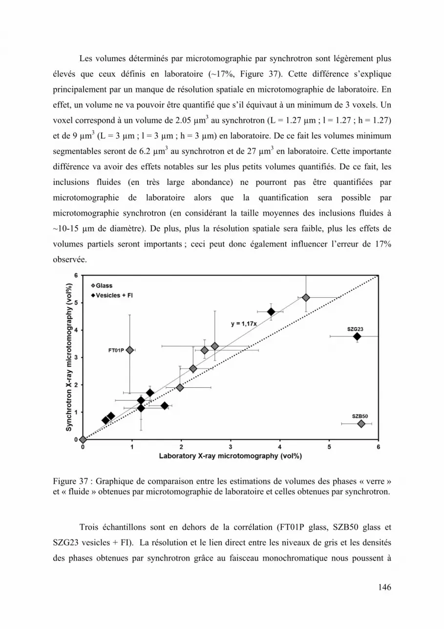
146

Les volumes déterminés par microtomographie par synchrotron sont légèrement plus

élevés que ceux définis en laboratoire (~17%, Figure 37). Cette différence s’explique

principalement par un manque de résolution spatiale en microtomographie de laboratoire. En

effet, un volume ne va pouvoir être quantifié que s’il équivaut à un minimum de 3 voxels. Un

voxel correspond à un volume de 2.05 µm3 au synchrotron (L = 1.27 µm ; l = 1.27 ; h = 1.27)

et de 9 µm3 (L = 3 µm ; l = 3 µm ; h = 3 µm) en laboratoire. De ce fait les volumes minimum

segmentables seront de 6.2 µm3 au synchrotron et de 27 µm3 en laboratoire. Cette importante

différence va avoir des effets notables sur les plus petits volumes quantifiés. De ce fait, les

inclusions fluides (en très large abondance) ne pourront pas être quantifiées par

microtomographie de laboratoire alors que la quantification sera possible par

microtomographie synchrotron (en considérant la taille moyennes des inclusions fluides à

~10-15 µm de diamètre). De plus, plus la résolution spatiale sera faible, plus les effets de

volumes partiels seront importants ; ceci peut donc également influencer l’erreur de 17%

observée.

Figure 37 : Graphique de comparaison entre les estimations de volumes des phases « verre » et « fluide » obtenues par microtomographie de laboratoire et celles obtenues par synchrotron.

Trois échantillons sont en dehors de la corrélation (FT01P glass, SZB50 glass et

SZG23 vesicles + FI). La résolution et le lien direct entre les niveaux de gris et les densités

des phases obtenues par synchrotron grâce au faisceau monochromatique nous poussent à

147

favoriser les données obtenues par cette méthode. Suivant cela, les quantités de verre de

FT01P semblent largement sous estimées par la microtomographie de laboratoire. A l’inverse,

les volumes de verre de SZB50 et de vésicules + inclusions fluides de SZG23 sont quant à

eux surestimés à largement surestimés pour SZB50. A l’heure actuelle aucune explication ne

peut être donnée quant à la variabilité des résultats obtenus entre les deux méthodes de

microtomographie sur ces 3 points.

La forte brillance des radiations synchrotron implique une nette supériorité en terme

de résolution spatiale et de ratio signal/bruit (Baruchel et al. 2006), mais le nombre limité

d’installation synchrotron et le coût élevé des analyses, diminue l’accessibilité. La

microtomographie à rayons X de laboratoire est quant à elle plus accessible mais a plus de

limitations en résolution. La microtomographie de laboratoire est donc un outil important

pour une approche préliminaire 3D des échantillons avant analyse synchrotron mais reste

limitée dans ses applications notamment par le manque de résolution spatiale et en densité.

148

5 Source du CO2 dans le Bassin Pannonien

Le Bassin Pannonien est une province pétrolière mature, qui a été intensément

explorée et faisant l’objet d’activité de production pétrolière et gazière depuis le début des

années 1930 (Dolton 2006). En Hongrie, plus de 5200 puits d’exploration ont été forés avant

les années 1990 (Kókai 1994), entrainant une connaissance accrue des fluides piégés dans les

différents sous bassins du Bassin Pannonien. La présence de CO2 en quantité importante dans

les champs de gaz a été identifiée assez tôt au cours de l’exploration du bassin, et initialement

associée à la décomposition thermique des carbonates du socle (Clayton et al. 1990),

notamment dans les sous-bassins de Bekes et de Zala. Certains champs de gaz dans ces

bassins, notamment à faible profondeur en bordure des hauts structuraux du socle, peuvent ne

contenir que du CO2 (Clayton et al. 1990). Les premiers travaux impliquant l’analyse

isotopique des gaz rares dans les années 90 (Sherwood Lollar et al. 1997; Ballentine 1997;

Ballentine et al. 1991) montrent de manière indiscutable l’origine mantellique du CO2 présent

dans une majorité de champs de la Little et de la Great Hungarian Plain. Ces travaux montrent

également l’importance localisée de sources crustales de CO2 (Sherwood Lollar et al. 1997).

Martel et al. (1989) ont également montré l’existence d’un flux mixte d’hélium mantellique et

crustal balayant l’essentiel du Bassin Pannonien, enregistré par l’abondance et la composition

isotopique de l’He des grands aquifères de la Great Hungarian Plain. L’association

systématique de l’3He et du CO2 dans les gisements de gaz, en proportion typiquement

mantelliques, et les flux remarquables d’3He dans les aquifères sont autant d’argument en

faveur d’un balayage de la lithosphère Pannonienne par des éléments volatils mantelliques.

Ces observations géochimiques sont en accord avec la présence d’un fort flux de chaleur au

niveau du bassin Pannonien, lié à la faible épaisseur de la Lithosphère, ainsi que de la longue

histoire volcanique ayant perdurée durant l’essentiel du Néogène (Huismans et al. 2002).

Afin de conforter ces travaux, nous avons souhaité compléter les données

géochimiques existantes sur les sources mantelliques des fluides dans le bassin Pannonien par

l’analyse d’aquifères riches en gaz connus dans notre zone d’étude de Bakony-Balaton. En

effet, une quantité importante de résurgences d’eau chargée en CO2, de sources thermales et

d’aquifères exploités pour la mise en bouteille d’eau gazeuse offrait une bonne opportunité

pour l’étude des flux de CO2 dans cette zone non investiguée par les études antérieures. Ces

travaux très préliminaires sur la géochimie de ces différents fluides visant à définir la

contribution mantellique des flux de CO2 affectant actuellement le BBHVF.

149

5.1 Traçage du CO2

Pour étudier la source du carbone il est primordial de connaître la nature de ses phases

porteuses et sa composition isotopique dans les différents réservoirs terrestres.

Figure 38 : Sources potentielles du CO2 en sub-surface. Source : [Cooper et al. 1997]

Les compositions isotopiques (δ13C) en carbone des différents réservoirs terrestres sont

comprises entre -115 ‰ et 25 ‰ (Figure 39). L’isotopie du carbone permet, dans la plupart

des cas, de discriminer les sources organiques des sources inorganiques (Cooper et al. 1997).

Les sources organiques sont majoritairement associées au CO2 provenant (1) de processus

biogéniques, (2) du craquage thermique du kérogène et (3) de la réduction thermochimique

des sulfates ; alors que les sources inorganiques sont quant à elles associées (1) au dégazage

du manteau terrestre, (2) aux réactions minérales associées au métamorphisme et (3) aux

réactions diagénétiques des phases minérales (Figure 38 ; Cooper et al., 1997).

A l’échelle inorganique, la composition isotopique du carbone est peu discriminante et

donc insuffisante à elle seule pour connaître la source du carbone. Par exemple, un δ13C de -

5‰ pourra être lié à une source mantellique, métamorphique ou diagénétique (crustale), qui

sont les trois sources principales de carbone intéressant cette étude.

150

Figure 39 : Variations des compositions en δ13C des différents réservoirs de carbone terrestre

Une discrimination entre les sources mantellique et crustale du CO2 inorganique est

possible grâce à l’isotopie de l’hélium couplée à celle du carbone. En effet, l’He a seulement

deux isotopes, l’3He et l’4He, le premier étant traceur d'une origine mantellique des éléments

volatils.

L’3He est très peu abondant par rapport à l’4He, de ce fait, il est devenu courant

d’utiliser le rapport isotopique d’He de l’échantillon, normalisé à celui de l’atmosphère :

R/Ra = (3He/4He)éch / (3He/4He)atm Avec Ra = 1,386.10-6 (atmosphère)

L’3He provient essentiellement de la nucléosynthèse primordiale aux premiers instants

de l’Univers, alors que l’4He est majoritairement d’origine radiogénique dans le manteau et

entièrement d’origine radiogénique dans la croûte. L’4He est le produit de la désintégration

radioactive de l’Uranium (U), du Thorium (Th) et dans une moindre abondance du Samarium

(Sm) (Moreira 2013). Il résulte de cela que le rapport R/Ra varie fortement entre les différents

réservoirs terrestres. Les sources mantelliques ont un R/Ra >> 1, reflétant un héritage d’3He

primordial (formation de la Terre). Une source crustale aura un R/Ra << 1, reflétant la nature

151

« dégazée » de la croûte (qui est le produit de la fusion du manteau), et sa forte teneur en

éléments radioactifs père de l’4He (U, Th). Le rapport isotopique de l’hélium ne se fractionne

pas lors des processus de fusion/cristallisation, ce qui fait donc de cet élément un bon traceur

de source dans les processus magmatiques (Figure 40).

Figure 40 : Evolution du rapport CO2/3He en fonction de : a- δ13C et b- CO2.

Sources : [a - Sano & Marty 1995; b- Sherwood Lollar et al. 1997]

Dans ce chapitre, on se propose d’étudier les gaz échantillonnés sur 4 captages

d’aquifère de le BBHVF afin de déterminer la source du CO2 présent dans cette zone du

Bassin Pannonien. Pour ce faire, des analyses de la composition des gaz, de l’isotopie du

carbone et des teneurs et isotopie en gaz rares ont été effectuées.

5.2 Échantillonnage des gaz d'aquifères

Pour notre étude, nous avons échantillonné les gaz associés à des aquifères peu

profonds dans 4 zones : Balantonfured, Badacsonyors et Kekkut (2 différents puits pour la

zone de Kekkut), en bordure Nord du Lac Balaton (Figure 27). Ces captages correspondent à

des résurgences naturelles (Balatonfured) ou à 3 puits de captage d’aquifères riches en gaz et

exploités pour la mise en bouteille (Badacsonyors, Kekkut 1 & 3).

L’échantillonnage s’est fait par un dispositif de dégazage des eaux en système fermé

directement sur le site de prélèvement (Figure 41).

a b

152

Figure 41 : Systèmes d’échantillonnages des gaz d’aquifères

1-Détecteur de Gaz, 2-Tube d’échantillonnage des gaz, 3-Bouteille de séparation eau/gaz

Le protocole d’échantillonnage est le suivant :

On introduit l’eau gazeuse dans la bouteille qui est initialement remplie d’air. Le flux

d’eau entrant dans la bouteille va chasser l’air par les tubes d’échantillonage, tout en dégazant

et en remplaçant le volume gazeux par les gaz initialement dissous dans l’eau. Un ciel de gaz

provenant de l’eau va se former dans la bouteille, qui pourra être collecté dans les tubes

échantillons. Afin de réduire au maximum la composante résiduelle en air dans le ciel de gaz,

un régime continu de circulation d’eau dans la bouteille est atteint en équilibrant la quantité

d’eau sortant de la bouteille par l’ajustement de la vanne de sortie. Le gaz s’accumulant dans

le ciel de gaz est progressivement évacué par les tubes d’échantillonage afin de chasser tout

air résiduel. Afin de suivre la diminution de la concentration en air et l’augmentation de la

concentration en gaz dissous dans le ciel de gaz du séparateur, nous utilisons un détecteur

directement relié à la sortie des tubes d’échantillonnage. La diminution d’O2 et

l’augmentation de CO2 sont les marqueurs du balayage de l’air par le gaz. L’O2 peut ne pas

diminuer jusqu’à 0%, dans ce cas-là, on considère que l’O2 est naturellement présent dans le

gaz si sa concentration reste stable malgré le balayage. Lorsque tout l’air a été balayé, il faut

piéger les gaz dans les tubes d’échantillonnage. Il est important de piéger le gaz avec une

pression maximale afin de faciliter les futures analyses en laboratoire. Le gaz a été pressurisé

153

(1,5 bars max) dans les tubes en jouant sur l’effet piston du flux d’eau dans la bouteille en

maintenant le tube fermé à sa sortie.

Les tubes d’échantillonnage de gaz sont constitués de cylindres en inox isolés par des

vannes en inox à obturation par pointeaux en Polychlorotrifluoroéthylène conçues pour

résister aux hautes pressions. L’étanchéité des tubes au vide et en pression est vérifiée au

laboratoire avant leur envoi en mission. Une fois ramenés au laboratoire, ces tubes sont

analysés successivement par chromatographie en phase gazeuse, puis sur une ligne d’analyse

des gaz rares. Un aliquote est également prélevé afin d’être analysé par GC-C-IRMS pour

mesurer la composition isotopique du carbone du CO2.

5.3 Techniques analytiques utilisées

5.3.1 Le GC-C-IRMS

La mesure de δ13C réalisée par couplage GC-C-IRMS (chromatographie en phase

gazeuse couplée à de la spectrométrie de masse de rapport isotopique) est identique à celle

proposée par Jeandel et al. (2010). Les molécules présentes dans le mélange gazeux (CO2 et

hydrocarbures de C1 à C5) sont séparées par une colonne Porabond Q de 27,5 m de long, de

0,32 mm de diamètre interne, de 0,45 mm de diamètre externe et d'épaisseur de film polymère

de 10 µm. Après séparation, les hydrocarbures sont transformés par combustion en CO2 et

H2O dans un four à combustion. Ces composés sont alors introduits dans la source du

spectromètre de masse où ils sont ionisés. Les ions 44 (12C16O2) et les ions 45 (13C16O2 + 12C16O17O) sont détectés et quantifiés afin de calculer le rapport isotopique 13C /12C des

molécules analysées. Ce rapport est ensuite comparé à celui d'un gaz de référence admis dans

la source du spectromètre (avant l’analyse) pour calculer le δ13CPDB (‰) par la formule

suivante:

δ13C =

1

CC

CC

ref12

13ech

12

13 * 1000

154

5.3.2 Le spectromètre de masse

L’étude des gaz rares est faite sur une ligne de purification couplée à deux

spectromètres de masse d’IFP Energies nouvelles. Cette ligne de purification sous ultravide a

été conçue afin d'analyser quantitativement les gaz rares (Hélium, Néon, Argon, Krypton) et

de mesurer les rapports isotopiques de l’He et de l’Ar. Les autres composés présents dans les

échantillons tels que le dioxyde de carbone, le méthane ou l'hydrogène sont purifiés sur deux

principes actifs : les réacteurs à mousse de titane et les Getter Zirconium-Aluminium. La

spectrométrie de masse quadripolaire (Pfeiffer Vacuum HiQuad) permet une mesure de la

composition élémentaire des gaz rares ainsi que la mesure du rapport 40Ar/36Ar. Le

spectromètre de masse à secteur magnétique (type VG 5400) permet de mesurer le rapport

isotopique de l’He. La ligne ultravide se décompose en trois grands secteurs : introduction,

purification et analyse. Le secteur d'introduction comprend le raccord des échantillons ainsi

que la zone d'ajustement de la pression d'introduction du gaz. Le secteur de purification est

divisé en deux lignes parallèles et symétriques, permettant de purifier deux échantillons en

même temps. Chacune des deux lignes de purification est composée de deux fours à mousse

de titane, d'un getter GP50, d'un piège cryogénique à charbon actif ainsi que d'une jauge

Pirani. Enfin, le secteur d'analyse se situe à la fin des lignes de purification, là où elles se

rejoignent, et comprend deux pièges cryogéniques à charbon actif et les spectromètres de

masse.

5.4 Résultats obtenus

Les résultats d’analyse sont fournis dans le Tableau 1. L’abondance relative des

éléments est représentée dans la Figure 42 où nous pouvons observer que les gaz sont

majoritairement composés de CO2 et de N2 (par ordre d’abondance). Les gaz contiennent

également des quantités non négligeables de méthane (<0,3%) et d’hélium (<0,4%).

155

Sample Kekkut 1 Kekkut 3 Badacsonyors Balatonfured

% % % %

N2 39,8 36,8 12,9 2,2

CO2 58,5 62,6 87,0 97,3

CH4 0,02 0,03 0,04 0,31 %o %o %o %o

δ13CO2 -8,773 -7,571 -6,2365 -5,985 ppm ppm ppm ppm 4He 3723 3912 393 14,6 +/- 94 147 15 0,44 20Ne 2,36 2,31 1,32 0,28 +/- 0,19 0,075 0,038 0,022 36Ar 10,1 11,5 6,96 2,00 +/- 0,11 0,072 0,041 0,014 84Kr 0,27 0,34 0,20 0,098 +/- 0,0093 0,0074 0,0041 0,0021 40Ar/36Ar 305,9 338,6 303,5 314,2 +/- 1,1 1,4 1,1 1,1 3He/4He 1,06E-06 9,83E-07 1,92E-06 2,68E-07 +/- 5,9E-08 3,8E-08 9,1E-08 4,5E-08

Tableau 1 : Analyses de gaz des échantillons de gaz d’aquifère de le BBHVF

Figure 42 : Abondance (mol%) des espèces majeures analysées

La Figure 43 représente les δ13C (δ13C = [13C/12C] / [1-Standard]) du CO2 en fonction

de l’inverse de l’abondance en CO2 de l’échantillon. Le δ13CO2 est compris entre -5,9 et -8,7

‰, indiquant une source inorganique du carbone.

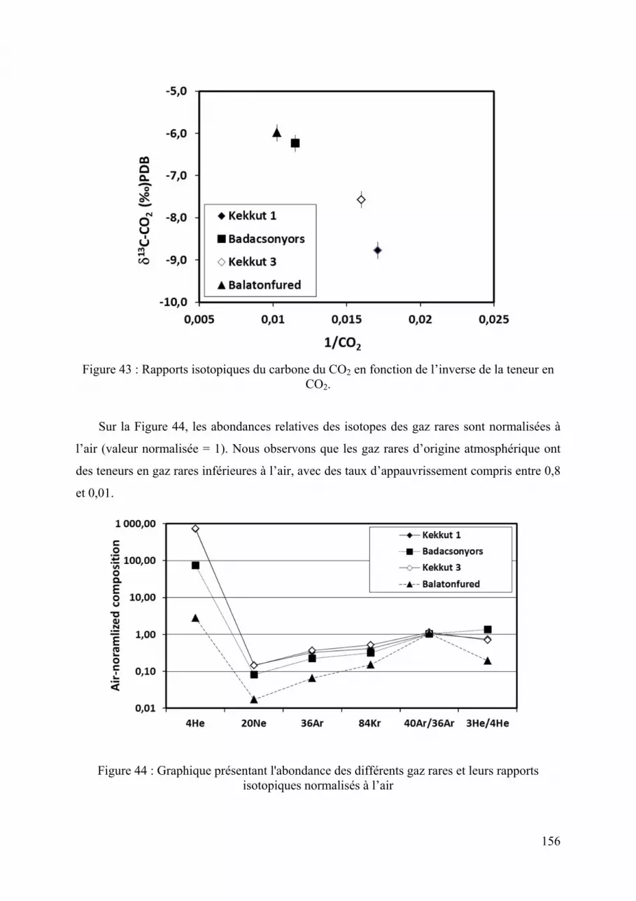
156

Figure 43 : Rapports isotopiques du carbone du CO2 en fonction de l’inverse de la teneur en CO2.

Sur la Figure 44, les abondances relatives des isotopes des gaz rares sont normalisées à

l’air (valeur normalisée = 1). Nous observons que les gaz rares d’origine atmosphérique ont

des teneurs en gaz rares inférieures à l’air, avec des taux d’appauvrissement compris entre 0,8

et 0,01.

Figure 44 : Graphique présentant l'abondance des différents gaz rares et leurs rapports isotopiques normalisés à l’air

157

Pour chaque échantillon, cet appauvrissement est inversement proportionnel à la

masse de chaque gaz rare, indiquant un effet de solubilité relative. L’hélium présente quant à

lui un enrichissement de 2,6 à 246,7 fois par rapport à l’air (soit jusqu’à 3910 ppm d’hélium).

Le rapport isotopique de l’Ar est compris entre 303,5 et 347,0 et présente un excès de 40Ar par

rapport à la valeur atmosphérique (295,5, Nier, 1950). Le rapport isotopique de l’hélium a une

plus grande variabilité avec des valeurs comprises entre 2,7.10-7 et 1,9.10-6, soit allant de

valeurs inférieures à supérieures par rapport à la référence atmosphérique (1,39.10-6, Ozima &

Podosek, 2002).

5.5 Discussion

Origine du CO2 et de l’azote

L’origine du CO2 succite de plus en plus l’intéret de chercheurs et d’entreprises

travaillant dans l’exploration d’hydrocarbure ou dans le stockage du CO2. De nombreuses

études sont donc sorties durant ces dernières années et présentent un couplage d’analyses

isotopiques du CO2 et de gaz rares, afin de déterminer les sources de ce CO2 (ex. : Gilfillan et

al. 2009; Jeandel et al. 2010). Par le même couplage, nous avons cherché à déterminer la

source du CO2 présent dans les aquifères superficiels de la BBHVF.

La composition isotopique du carbone du CO2 (13CCO2) comprise entre -5,9 et -8,7‰

correspond à une origine inorganique du CO2 (Cooper et al. 1997), en accord avec la gamme

des valeurs mesurées par Sherwood Lollar et al. (1997) et Ballentine et al. (1991) sur les gaz

du bassin Pannonien. De plus, les rapports isotopiques de l’hélium compris entre 0,4 et 1,2 Ra

(R/Ra= 3He/4Heech/3He/4Heatm) pour des rapports 20Ne/4He supérieurs à 1.10-4 impliquant une

contribution d’hélium profond depuis des sources à la fois mantelliques et crustales (Figure

45). Les rapports CO2/3He de nos échantillons de gaz s’échelonnent entre 1,5.108 et 2,5.1011

et sont dans la gamme haute des mêmes rapports déterminés par Sherwood Lollar et al.

(1997), correspondant aux échantillons présentant de fortes teneurs en CO2, typiquement

supérieures à 10 mol.%. Il est à noter que seules les abondances en CO2 et CH4 sont données

dans Sherwood Lollar et al. (1997), valeurs fournies par les compagnies pétrolières opérant

les puits échantillonnés. Il n’est pas mentionné dans cet article la présence éventuelle de N2

dans les échantillons, ce qui limite l’intérêt d’une comparaison des compositions élémentaires

158

avec nos échantillons. En revanche, Ballentine et al. (1991) montrent une importante fraction

de N2 dans deux champs de la Great Hungarian Plain, jusqu’à 30 mol.%. Si on s’affranchit du

N2, l’essentiel de nos échantillons est constitué de CO2, ce qui placerait l’ensemble de nos

échantillons sur l’extrême droite de la corrélation entre CO2/3He et CO2 de Sherwood Lollar

et al. (1997), entre le pôle MORB et un pôle crustal (Figure 45).

Figure 45 : a- Graphique présentant le rapport CO2/3He en fonction du CO2 (Mol%).; b-

Graphique présentant le rapport isotopique 20Ne/4He en fonction de 3He/4He. Source : [a-

Sherwood Lollar et al. 1997 ; b- Sherwood Lollar et al. 1997; Ballentine et al. 2001]

L’azote moléculaire présente en quantité importante dans nos échantillons est corrélé

avec l’abondance en gaz rares atmosphériques (20Ne, 36Ar et 84Kr), et présente des rapports

N2/36Ar s’échelonnant entre la valeur de l’air et des valeurs supérieures à une eau équilibrée

avec l’air (AEW). Les échantillons comportant des rapports N2/36Ar compris entre l’air et

AEW (Badacsonyors, Balatonfured) sont vraisemblablement constitués d’azote purement

atmosphérique, plus ou moins fractionnés de l’Ar par des processus de solubilité. Les

échantillons présentant des excès de N2 par rapport à AEW (Kekkut 1 et 3) nécessitent

d’invoquer une source d’azote additionnelle. Les aquifères de Kekkut et de Badacsonyors ont

donc vraisemblablement accumulé de l’azote non atmosphérique. L’abondance en N2 montre

une corrélation forte avec l’abondance en 4He (Figure 46), dont l’origine est clairement un

mélange entre une source mantellique et une source crustale. Il y a fort à penser que l’azote

non atmosphérique dans ces aquifères est d’origine profonde, comme il a déjà été démontré

pour les résurgences hydrothermales du Rift d’Eger en Europe Centrale (Weinlich et al.

1999), pour lesquelles du CO2 d’origine magmatique est associé à du N2 d’origine

probablement métamorphique.

a b

159

Figure 46 : Corrélation entre N2 et 4He pour les échantillons de gaz de le BBHVF.

Correction des effets de dégazage

Les fluides naturels prélevés ici correspondent à des aquifères chargés en gaz. Le mode

de résurgence, ou de captage de ces fluides implique un dégazage de ces eaux au cours de leur

remontée vers la surface. De plus, la méthode d’échantillonnage présentée plus haut pousse ce

dégazage jusqu’à un équilibre de solubilité correspondant à la pression atmosphérique, et à la

température de l’eau à l’exutoire. Cette dynamique dans les équilibres de phase fluide lors de

la remontée et l’échantillonnage de ces eaux implique nécessairement un fractionnement

compositionnel des différents composés volatils entre la phase liquide et la phase vapeur. Afin

de remonter à une information correspondant à l’état compositionnel du système dans

l’aquifère, voire à son état de phase (monophasique, diphasique), ces fractionnements doivent

être corrigés. Pour ce faire, nous allons mettre en œuvre un calculateur exploitant une

équation d’état développé à IFPEN sur la base du modèle de Soreide & Whitson (1992), qui

permet d’étudier l’état de phase fluide de systèmes complexes H2O-NaCl-N2-O2-H2-CO2-

CH4-H2S. Afin d’exploiter ce calculateur dans le but de reconstituer l’état du système fluide

dans l’aquifère, il nous faut faire un certain nombre d’hypothèses sur 1) la pression

hydrostatique de l’aquifère (donc sa profondeur et sa charge artésienne le cas échéant), 2) un

point de référence compositionnel du système, ou les rapports volumiques eau/gaz à

l’exutoire. Ce deuxième point permet d’ancrer la composition du système à un bilan de masse.

160

Grace à ce calculateur, nous nous intéresserons à déterminer la composition d’une eau à

l’origine des gaz échantillonnés, en faisant un calcul inverse de dégazage. Pour ce calcul, la

pression de dégazage est celle de la surface, soit 1 bar. Nous prenons ensuite pour référence

compositionnelle la teneur en gaz rares atmosphériques, assimilée à l’équilibre de l’eau avec

l’air à 1 bar et à une température de surface moyenne annuelle (10°C), sans excès d’air, et

sans oxygène (ci-après AEW pour air-equilibrated-water). Cette composition est une

hypothèse satisfaisant le cas le plus général pour des aquifères situés sous la nappe phréatique

(déjà en anoxie). Cette référence compositionnelle permettra d’utiliser les gaz rares dits

« atmosphériques » (20Ne, 36Ar, 84Kr), ainsi que l’azote atmosphérique associé (N2atm) pour

déterminer la contribution de l’eau à la composition du système (Ballentine et al. 1991). Tout

composé en excès par rapport à cette référence correspond à l’ajout d’un constituant dans

l’aquifère. Le calculateur pouvant fidèlement calculer le fractionnement de ces constituants de

référence entre la phase liquide et la phase vapeur pour tous les équilibres, la concentration de

ces composés atmosphériques dans la phase vapeur (donc la phase que nous analysons dans

cette étude) permet de déduire l’abondance de la composante AEW dans le système aquifère,

par rapport à une composante dite excédentaire. La composante excédentaire dont on cible ici

la détermination est le CO2, ainsi que l’He.

Tableau 2 : Composition des eaux à l’origine des gaz échantillonnés dans les aquifères par un

calcul inverse de dégazage (cf. texte). f- final, i- initiale.

CO2/3He N2/

36Ar 4He/36Ar CO2 (mol.%)

water f 1,44E+10 14177 77,7 98,6

water i 1,95E+09 25316 233,7 94,3

gaz f 1,68E+08 32021 327,6 61,3

Kekkut 1 1,63E+08 32029 340,3 62,6

water f 1,15E+11 7769 12,1 99,7

water i 8,84E+09 15579 44,8 97,9

gaz f 1,15E+09 18178 55,7 86,9Badacsonyrs 1,15E+09 18583 56,5 87,0

water f 2,53E+13 4684 1,6 100,0water i 6,61E+11 10516 6,8 99,1

gaz f 2,54E+11 10959 7,2 97,8Balatonfured 2,49E+11 10872 7,3 97,3

161

En pratique pour ces calculs, on se place dans un système initial monophasique composé

d’une eau de type AEW. On va doper cette eau avec des teneurs en CO2 et en He afin

d’obtenir, pour un équilibre à 1 bar et une T de 10°C, une phase vapeur de composition

moléculaire correspondant à un échantillon analysé. On procède par itération afin d’ajuster la

composition initiale du système. Etant donné la multiplicité des paramètres compositionnels

calculés, nous nous basons sur différents critères pour caler le système. Ces paramètres sont :

N2/36Ar, 4He/36Ar, CO2/

3He. Les résultats de ces calculs sont fournis dans le

Tableau 2, en comparaison avec les analyses des gaz d’aquifère de le BBHVF. Pour

chaque exemple de calcul, on donne la composition du système initial, et la composition des

deux phases vapeur et liquide à l’équilibre (1 bar, 10°C).

Figure 47 : Importance des processus de dégazage dans l’évolution des compositions des fluides au cours des interactions eau-gaz. a- Graphique présentant le rapport CO2/

3He en fonction du CO2 (Mol%) ; b- Graphique présentant le rapport CO2/

3He en fonction du rapport 4He/36Ar ; c- Graphique présentant le rapport N2/

36Ar en fonction du rapport 4He/36Ar. Wi – composition initiale de l’eau avant dégazage, composition calculée ; Wf – composition finale de l’eau après dégazage, composition calculée ; Gf – composition finale du gaz, composition calculée similaire à la composition mesurée.

a b

c

162

Les compositions initiales calculées tendent vers des eaux légèrement à fortement

sursaturées en CO2, pour lesquelles les rapports CO2/3He sont plus forts que ceux mesurés

dans les gaz (Figure 48, Tableau 2). Ce résultat est attendu et correspond bien à l’inversion de

l’effet de dégazage. Les itérations ont mené à enrichir l’eau également en N2, du fait de

rapports N2/36Ar excédentaires par rapport à AEW dans les échantillons. L’amplitude de

l’effet de dégazage est remarquable sur certains rapports, allant jusqu’à plus d’un ordre de

grandeur pour le CO2/3He et jusqu’à 80% pour le 4He/36Ar (Figure 47). D’une manière

générale, on observe que la phase liquide perd l’essentiel de l’He et du N2, et retient une

quantité importante de CO2. Inversement, la phase vapeur, est relativement enrichie en He et

en N2, et appauvrie en CO2. Le bilan de masse sur le dégazage des eaux de Kekkut implique

que 95% du CO2 de la phase initiale reste dans la phase liquide, et que par conséquent la

phase vapeur ne véhicule qu’une fraction, minoritaire du CO2 présent dans le système initial.

Le taux de dégazage de l’aquifère peut-être généralement corrélé au rapport 20Ne/36Ar, qui

tend depuis des valeurs faiblement dégazées typiquement atmosphériques (0,52), vers des

valeurs totalement dégazées de type AEW (0,15).

Figure 48 : Graphique présentant le rapport CO2/3He en fonction du CO2 (Mol%) présentant

les compositions initiales recalculées.

163

Dans la suite de ce chapitre, nous exploiterons les compositions issues des corrections

de dégazage comme représentatives des fluides naturels présents en subsurface. En ce qui

concerne les compositions isotopiques, nous considérerons les valeurs des gaz échantillonnés

comme représentatives des fluides profonds. Cette considération est vraisemblablement

valable pour l’He et l’Ar dont les rapports isotopiques se fractionnent peu du fait des effets de

solubilité, mais elle est discutable pour le carbone du CO2 (Clark & Fritz 1997). En effet, le

13CCO2 peut fortement varier lors d’équilibre eau-gaz dans des aquifères ou dans des

réservoirs de gaz (Deines et al. 1974; Gilfillan et al. 2009).

Sources multiples et/ou mélanges de fluides variablement dégazés ?

Le calcul d’inversion des effets de dégazage montre l’importance de ces processus

dans l’évolution des compositions des fluides au cours des interactions eau-gaz dans les

niveaux aquifères au cours de leur remontée vers la surface. De tels effets ont déjà été reportés

par Ballentine et al. (1991) sur des gaz du bassin Pannonien, mais exclusivement sur les gaz

rares. Nos résultats impliquent une sous-estimation des rapports CO2/3He importante (Figure

47) lorsque l’on ne considère que l’analyse de la phase gaz. Les fluides corrigés du dégazage

corrèlent plus fortement avec les échantillons étudiés par Sherwood Lollar et al. (1997), et

couvrent l’ensemble des valeurs de CO2/3He des gaz caractérisés par CO2>95 mol.%, soit

entre 1,5.108 et 6,5.1011. La forte hétérogénéité des rapports CO2/3He rapportée par Sherwood

Lollar et al. (1997), corrélée à la variabilité des rapports 3He/4He et des teneurs en CO2, se

manifeste à l’échelle de l’ensemble du bassin Pannonien. Bien que dans le cadre de notre

étude les teneurs en CO2 soient moins variables et caractérisées par de fortes teneurs, la

variabilité importante des rapports CO2/3He reste surprenante vue la faible étendue spatiale de

notre zone d’étude. De plus, les échantillons d’aquifère de le BBHVF montrent une forte

dépendance compositionnelle à leur taux de dégazage. Notamment, les calculs de correction

de dégazage montrent un lien potentiel entre les échantillons les plus dégazés et les

échantillons les moins dégazés. Les échantillons correspondant aux plus faibles taux de

dégazage (Kekkut 1 et 3) sont caractérisés par de faibles rapports CO2/N2, CO2/3He et δ13C,

ainsi que de forts rapports 4He/36Ar et 3He/4He. Inversement, les échantillons issus des plus

forts taux de dégazage (Badacsonyors et Balatonfured) sont caractérisés par de forts rapports

CO2/N2, CO2/3He et δ13C, ainsi que de faibles rapports 4He/36Ar et 3He/4He (Tableau 1).

164

La forte affinité avec une origine proprement mantellique des échantillons de Kekkut

(3He/4He=0,8Ra, CO2/3He=1,5.108) leur confère un caractère primaire, à savoir peu modifié

par des processus de mélange et de fractionnement physique. Leur teneur enrichie en N2 à

priori crustal, ainsi que leur composition isotopique d’He montrant une composante

radiogénique importante, implique que ces fluides primaires correspondent à un mélange

entre une source de CO2 mantellique et une source de N2 métamorphique, avec leurs cortèges

d’He associés. Ce type de fluide semble similaire à ceux décrits dans le Rift d’Eger (Weinlich

et al. 1999), et potentiellement ceux des champs de CO2 de la Little Hungarian Plain

(Sherwood Lollar et al. 1997). L’échantillon de Balatonfured montre une plus forte affinité

crustale, avec des 3He/4He = 0,2 Ra et des CO2/3He de 2,5.1011. En revanche, cet échantillon

est dépourvu d’azote non atmosphérique et présente des rapports 4He/36Ar faibles (Tableau 1).

L’échantillon de Badacsonyors a des caractéristiques intermédiaires entre les échantillons de

Kekkut et celui de Balatonfured. Nous présentons ici deux scénarii permettant d’expliquer les

hétérogénéités des caractéristiques de ces fluides sur une zone de si faible étendue

géographique.

Le premier scénario implique l’existence de deux pôles de fluide ; (1) un fluide

d’origine mantellique riche en CO2 de 13CCO2 entre -8‰ et -5‰, comportant une composante

d’azote et d’He crustal, (2) un fluide ayant pour origine la décarbonatation de niveaux

sédimentaires ou métamorphiques de 13CCO2 = -5‰, associé à de l’He radiogénique et

dépourvu d’azote. Au grès des chemins de remonté, partiellement indépendants de ces deux

sources de fluide, les aquifères de le BBHVF se chargent de manière variable en ces deux

composantes, exprimant les hétérogénéités compositionnelles observées.

Le deuxième scénario implique une seule source de CO2 d’origine mantellique de

13CCO2 = -5‰ associée à de l’azote et de l’He crustal. Dans ce scénario, le cheminement du

fluide profond vers la surface est associé à des fractionnements physiques importants dus à de

multiples équilibres de phase eau-gaz. Les phases gaz primaires parvenant à sursaturer les

différents niveaux aquifères jusqu’à des niveaux superficiels lors de leur remontée préservent

des caractéristiques géochimiques proches de la source profonde. Ces flux gazeux primaires

atteignent les aquifères superficiels correspondants aux échantillons de Kekkut. Les systèmes

d’aquifères ayant été saturés par ce flux gazeux sont comparativement appauvris en He et en

N2, et expriment des rapports CO2/3He élevés, ainsi que des teneurs en He profond faibles.

L’incorporation de ces masses d’eau riches en CO2 dans des systèmes convectifs de régimes

165

hydrothermaux sont acheminés vers la surface en se mélangeant avec des recharges

météoriques de grande amplitude ayant incorporées de l’He radiogénique à la faveur des

lithologies traversées. Dans des conditions favorables de mélange avec ces recharges

météoriques, ces flux secondaires peuvent atteindre leur point de bulle et générer des gaz

présentant des rapports CO2/3He élevés, et des faibles teneurs en He de nature plus

radiogéniques (échantillon de Balatonfured). Selon les conditions de dégazage de ces

différents flux en surface (résurgences, dégazages diffus), l’expression des caractéristiques

primaires et secondaires de ces fluides se distinguent localement.

Bien qu’il soit difficile dans l’état actuel d’avancement de ces travaux de trancher

entre ces deux scenarii, il est clair que l’effet d’équilibre gaz-eau dans ce type de contexte

semble essentiel à considérer. En effet, les fractionnements d’équilibre eau-gaz pour le CO2,

l’He et le N2 sont concordants avec le deuxième scénario. Sans qu’une démonstration ne

puisse être donné à présent sur ce point, les différences de composition isotopique du carbone

du CO2 (Figure 43) ne sont pas incompatibles avec un fractionnement lié à des effets de

solubilité tels que montrés par Gilfillan et al. (2009) sur des accumulations de CO2 en

Amérique du Nord. Il semble difficile dans l’état actuel des choses de justifier un 13CCO2 = -

8‰ pour une source mantellique, si ce n’est en invoquant un mélange impliquant une faible

contribution thermogénique de CO2 (13CCO2 ~ -25‰) pour laquelle peu d’arguments existent

(Clayton et al. 1990). Le scénario 1, en revanche, semble plus en accord avec les travaux de

Sherwood Lollar et al. (1997) et Clayton et al. (1990), bien que les effets de fractionnement

invoqués dans le scénario 2 n’y aient pas été investigués. Ces effets ont pourtant bien été

démontrés dans le bassin Pannonien par Ballentine et al. (1991) sur la base de

fractionnements élémentaires entre les gaz rares.

Une campagne d’échantillonnage plus complète ainsi que des travaux plus aboutis sur

la modélisation des effets compositionnels et isotopiques d’interactions gaz-eau devrait

permettre de trancher entre ces deux scénarii.

166

5.6 Conclusions

Des échantillons de gaz provenant d’aquifères captés dans le BBHVF (Kekkut,

Badacsonyors, Balatonfured) montrent de fortes teneurs en CO2 (58 à 97%), complétées par

du N2 en proportion s’échelonnant entre 40 et 2 mol.%. Le CO2 porte une composition

isotopique du carbone entre -8 et -6 ‰ (13CPDB) typique d’une origine inorganique. La

composition élémentaire et isotopique en hélium pointe vers une origine proprement

mantellique pour les échantillons de Kekkut et Badacsonyors, et plus probablement crustale

pour Balatonfured. Une composante crustale de N2 est déduite à partir de l’identification

d’excès de N2 par rapport au pôle météorique. L’étude des fractionnements élémentaires liés

aux interactions gaz-eau indique cependant que ces différents sites d’échantillonnage

pourraient avoir une source commune de CO2 mantellique, exprimant des caractéristiques

géochimiques hétérogènes au grès de chemins et modes de migration variables. Ces travaux

préliminaires confirment les travaux antérieurs ayant montré l’existence d’un flux de CO2

mantellique dans différentes zones du bassin Pannonien (Martel et al. 1989; Sherwood Lollar

et al. 1997; Ballentine 1997). Ces nouvelles données géochimiques de gaz permettent de

préciser la nature du CO2 balayant les aquifères de le BBHVF, une zone qui n’avait pas

encore été explorée de ce point de vue. La position particulière de le BBHVF dans le bassin

Pannonien, situé en bordure du grand système transformant de la Mid Hungarian Zone sur des

niveaux affleurant du socle, indique un flux actuel important de CO2 vraisemblablement guidé

par des systèmes de failles profondes.

167

6 La migration du CO2 : du manteau au bassin Pannonien

6.1 Le bassin Pannonien – une zone géodynamique favorable aux

migrations lithosphériques de fluides mantelliques

De fortes teneurs en CO2 ont été quantifiées dans le manteau situé sous le bassin

Pannonien (~2000 ppm, cf. Le carbone dans le manteau sous Pannonien) et dans le bassin

Pannonien à travers les flux de CO2 mantellique dans les aquifères superficiels (cf. Source du

CO2 dans le Bassin Pannonien) et dans les réservoirs pétroliers et gaziers (Sherwood Lollar et

al. 1997). La corrélation observée entre CO2 (%) et CO2/3He (Figure 48) dans le bassin peut

être expliquée par des processus ayant lieu au cours de la migration tels que : (1) la perte de la

phase porteuse du CO2 mantellique (fractionnement physique); (2) l’ajout de CO2 crustal; (3)

l’ajout de CH4 crustal; et potentiellement (4) la conversion du CO2 mantellique en CH4

(Sherwood Lollar et al. 1997). Ces différents processus peuvent se produire sur des échelles

de temps et d’espace considérables, typiquement géodynamiques. La compréhension des

processus de migrations qui lient le réservoir mantellique et les niveaux de roches

sédimentaires du bassin est donc primordiale.

La subduction de la lithosphère européenne a eu lieu entre l’Eocène et le Miocène

(Martin & Németh 2004) et serait associée à la mise en place des édifices calco-alcalins

observés à la surface du bassin Pannonien. L’étude des xénolites mantelliques de le BBHVF,

remontés par le volcanisme alcalin entre la fin du Miocène et le début du Pliocène, a montré

que la subduction a fortement enrichi le manteau en éléments volatils et notamment en CO2

durant cette période. En effet, nous avons pu montrer que les magmas percolant les péridotites

lithosphériques provenaient très probablement de la fusion de la lithosphère subductante et

qu’ils pouvaient contenir jusqu’à 25.4 wt. % de CO2. Il est donc aisé de penser que la

lithosphère européenne a libéré de très grandes quantités de CO2 durant sa subduction sous la

zone Carpato-Pannonienne (Eocène-Miocène). La présence de fluides en grandes quantités

dans la lithosphère subductante a impliqué la libération de grandes quantités de CO2 ainsi que

la diminution des conditions de stabilité de nombreuses phases (diminution du solidus) et

donc la formation de magmas. Ce mécanisme en chaîne à notamment pu accélérer la

déformation du manteau et de la croûte par la génération de magmas et l’injection de volatils.

168

Figure 49 : Résumé des interactions fluide-roche pouvant avoir lieu à l’échelle lithosphérique. Les bandes hachurées représentent les niveaux marbrés. Les deux fines flèches décrivent des intéractions fluide-roche (infiltrations de H2O-CO2 ou dévolatilisation liée au métamorphisme), les flèches épaisses décrivent les infiltrations majeures de fluides. La position structurale à l’intérieur ou à l’extérieur des zones de cisaillement majeur ou mineur exerce un contrôle majeur sur la nature des fluides et sur leurs flux. Plusieurs de ces processus peuvent être caractéristiques de la lithosphère Pannonienne et sont discuttés dans le texte. Source : [Pili et al. 1999]

La majorité des gaz libérés par dégazage non-magmatique, circule principalement par

les failles et/ou fractures (Figure 49). De ce fait, la tectonique joue un rôle important dans les

processus de dégazage (e.g. Gold 1993; Irwin & Barnes 1980). Pili et al. (1999) résument les

processus de source et les circulations lithosphériques de CO2 résultantes. Ils montrent

notamment que les zones de cisaillement exercent un contrôle majeur sur la nature des fluides

et sur les flux. Ainsi les zones de cisaillement majeures prélèvent du CO2 mantellique (et

crustal) et libèrent des flux équivalent à ceux observés au niveau des rides océaniques.

169

Figure 50 : Carte illustrant la profondeur du socle du bassin Pannonien ainsi que les failles majeures contrôlant la formation du bassin. 1- avant arc ; 2- ceinture de flysch ; 3- volcans Miocène et positions approximatives des centres éruptifs explosifs (dépôts rhyolitiques) ; 4- Montagnes alpines, des Carpates et dinariques ; 5- Fenêtre Apenninique ; 6- Ophiolites ; 7- failles normales et de détachement ; 8- Déformations anticlinales ; 9- Failles de décrochement ; 10- failles de décrochement de premier ordre ; AC- Plaque Alcapa; MHFZ- Mid-hungarian zone ; TD- Plaque Tisca-Dacia. Source : [Horváth et al. 2015].

Le bassin Pannonien a subi une histoire géodynamique complexe passant de phases

compressives à extensives à plusieurs reprises. Cette histoire complexe a mené à la formation

de nombreuses failles qui sont présentées sur la Figure 50. Une structure majeure est

d’ailleurs bien visible au centre du bassin Pannonien (Figure 50), c’est la Mid-Hungarian

Zone (MHZ). La MHZ est composée d’une série de failles parallèles et lithosphériques. Elle

est décrite dans la littérature comme un système décrochant datant de l’Oligocène, et le long

duquel les micro-plaques ALCAPA et TISZA-DACIA se juxtaposent (ex. : Géczy 1973;

Géczy 1984; Kovacs 1982; Csontos et al. 1992). Cette forte zone de cisaillements

lithosphériques concorde d’un point de vu temporel avec la subduction de la lithosphère

européenne. De plus, l’ensemble de la longueur du système de la MHZ est recouverte par

170

d’épais dépôts volcaniques calco-alcalins datant du Miocène (Balla 1984; Balla 1987).

Weinlich et al. (1999) expliquent que les chemins de migration des magmas sont également

des chenaux utilisés par les fluides (ex. : le CO2) pour migrer vers la surface (Figure 50). Il est

donc aisé de penser que les fluides libérés lors de la subduction ont pu facilement migrer vers

le bassin et la surface par les failles lithosphériques formant la MHZ au cours de l’Oligocène

et du Miocène. En accord avec ces hypothèses, les analyses des gaz du bassin Pannonien

montrent que les plus fortes concentrations en CO2, associées à une origine mantellique, sont

localisées sur/à proximité de la MHZ, dans la Great Hungarian Plain (Sherwood Lollar et al.

1997) et dans le BBHVF (cette étude). Ces observations s’accordent donc avec une migration

de fluides mantelliques riches en CO2 libérés par la subduction de la plaque européenne, vers

le bassin sédimentaire et, par les failles lithosphériques et les chemins de migration des

magmas calco-alcalins de la MHZ.

Figure 51 : Exemple de synopsis des sources de CO2, He et N2, leurs signatures isotopiques, les processus de transport et de mélange dans l’Ouest du rift Eger. Source : [Weinlich et al. 1999]

Sacchi & Horváth (2002) ont montré que bien que la zone Carpato-Pannonienne ait été

soulevée entièrement au cours du Quaternaire, des mouvements verticaux différentiels

indiquent une flexure continue avec un soulèvement maximal entre le BBHVF (Bakony) et le

mont Mecsek (Figure 52, Cloetingh et al., 2006). Cette information est importante car elle

montre que le BBHVF se situe en bordure de bassin et à proximité des pentes de flexions

171

maximales. Cette perte de rigidité est liée aux transitions de phase et à la migration

d’éléments volatils associés (Morner & Etiope 2002) dans les zones de forte fracturation.

Plusieurs des principaux champs pétroliers et gaziers mondiaux sont localisés dans des

bassins ayant subi une perte de rigidité de la lithosphère (Morner & Etiope 2002). Dans ces

bassins (ex. : l’Est des Carpates, la Mer Noire, le Péri-Caspien), les accumulations d’éléments

volatils mantelliques (ex. : CO2) ne se font pas dans le centre du bassin mais plutôt le long des

pentes de flexion maximale où la lithosphère doit avoir perdue sa rigidité normale. De ce fait,

la localisation de le BBHVF, à proximité de zones de flexion maximale de la lithosphère,

favorise une libération importante de fluide qui est en accord avec les teneurs en CO2

mantellique observées dans les aquifères de cette zone.

Figure 52 : Exemple de plissement à l’échelle crustale en Transdanubie (Hongrie), basée sur l’interprétation et l’analyse de séquences stratigraphiques de profils de réflexion sismique régionale (Sacchi & Horváth 2002). Source : [Cloetingh et al. 2006]

Nous proposons donc une migration du CO2 mantellique par flux advectif le long des

chemins de migration de magmas présents dans le bassin Pannonien mais surtout, une

migration diffuse de ce CO2 le long des différents plans de failles associés à la mise-en-place

du bassin (Figure 53), controlée en partie par la MHZ.

172

Figure 53 : Chemins de migration du CO2 mantellique, vers le bassin Pannonien, par flux advectifs et par migration diffuse le long des différents plans de failles associés à la mise-en-place du bassin.

6.2 Perspectives de ces travaux de thèse

De fortes teneurs en CO2 ont été quantifiées dans le manteau situé sous le bassin

Pannonien (~2000 ppm, cf. Le carbone dans le manteau sous Pannonien) et dans le bassin

Pannonien à travers les flux de CO2 dans les aquifères superficiels (cf. Source du CO2 dans le

Bassin Pannonien). De plus, de nombreuses évidences de la présence de CO2 ont été décrites

dans la croûte Pannonienne par l’étude d’enclaves crustales remontées par le volcanisme

alcalin (ex.: Kempton et al. 1997; Török et al. 2005). Nous cherchons donc à définir les

processus qui lient ces réservoirs d’un point de vu spatio-temporel ; pour cela, la définition

des flux de CO2 est primordiale.

173

Dans le chapitre précédent, nous avons pu voir que les gaz rares sont des outils

puissants pour le traçage de source. Dans ce paragraphe, nous allons également démontrer

leur importance dans la détermination des flux de gaz.

Le premier objectif est la définition du pôle mantellique du bassin Pannonien et

d’investiguer les potentiels mélanges ayant pu avoir lieu entre la croûte subductée et le

manteau (cf. Pétro-géochimie du manteau Pannonien). Pour cela, nous proposons de broyer

sous vide les xénolites mantelliques étudiés au cours de cette thèse afin d’extraire l’ensemble

des éléments volatils qu’ils piégeaient. L’analyse du carbone et des gaz rares associés sera

alors faites à l’aide d’un couplage entre un spectromètre de masse quadripolaire et un

spectromètre de masse à secteur magnétique. L’utilisation de ce couplage, permettra par le

biais d’une seule analyse, de mesurer les concentrations en carbone et gaz rares, ainsi que

l’isotopie des gaz rares. L’ensemble des résultats permettra alors de définir précisément le

pôle mantellique du bassin Pannonien et les potentiels mélanges entre la croûte subductée et

le manteau. En effet, la présence d’un mélange entre un pôle crustal et un pôle mantellique

impliquerait des compositions appauvries en 3He/4He et enrichies en CO2/3He par rapport à un

pôle MORB (Marty et al. 1989; MacPherson et al. 2010; Pinti & Marty 2000).

La définition des teneurs en CO2 et gaz rares ainsi que l’isotopie de ces derniers dans

les xénolites crustaux (échantillonnées au cours de cette thèse) permettra l’estimation des

gains/pertes en CO2 des fluides au cours de leur migration vers la surface (dans le manteau,

par le biais des xénolites mantelliques ; dans la croûte, par le biais des xénolites crustaux ; et

dans le bassin à différentes profondeurs par le biais des réservoirs gaziers et des aquifères).

L’3He étant primordial, il ne peut y avoir d’ajout de cet isotope au cours de la migration

des fluides. Le fractionnement élémentaire du rapport CO2/3He au cours des processus de

fusion/migration nous servira donc de traceur des bilans de masse de CO2 depuis le manteau

jusqu’au bassin. Une augmentation du rapport CO2/3He par rapport à celui du manteau

(typiquement 1 à 3.109), s’expliquera par un apport supplémentaire de CO2 (Sano & Marty

1995), via des contributions crustales, sédimentaires ou organiques. A l’inverse, une

diminution de ce rapport par rapport au pôle mantellique s’expliquera par une perte de CO2 au

cours de la migration (Sherwood Lollar et al. 1997), résultant des réactivités et solubilités très

contrastées de l’He et du CO2.

174

Certains aquifères de la Great Hungarian Plain (GHP), dans le bassin Pannonien ont

aussi fait l’objet d’analyse d’3He (Martel et al. 1989). En principe, les flux d’He mantellique

et crustal (radiogénique) peuvent être estimés si les caractéristiques de l’aquifère sont

connues. Par la prise en compte de l’hydrogéologie de ces aquifères et de leurs teneurs en 3He, Martel et al. (1989) ont pu calculer des flux, fournissant des valeurs de 15 cm3.s-1 pour le

flux d’hélium mantellique et de 35 m3.s-1 pour le débit d’eau dans les aquifères. Le système

aquifère de la GHP a une surface de 50000 km², le flux d’hélium mantellique de 15 cm3.s-1

correspond alors à ~8.104 atom. m-².s-1.

Les longs chemins de migration entre le manteau et la surface impliquent un passage des

gaz mantelliques dans plusieurs systèmes hydrologiques. Au cours de la traversée de ces

systèmes, des équilibres eau/gaz peuvent se mettre en place. Il est communément admis que le

CO2 s’équilibre isotopiquement dans tous les systèmes hydrologiques qu’il traverse. De tels

effets de fractionnements par étapes ne peuvent pas être prouvés pour tous les équilibres, car

seul le processus le plus superficiel sera disponible pour le calcul de bilan de masse.

L’hélium, quant à lui, ne réagit pas chimiquement avec les composants de l’eau, et son

fractionnement isotopique est beaucoup moins important que pour le CO2 lors de la traversée

des systèmes hydrologiques. Des changements de composition chimique ou isotopique

peuvent être expliqués seulement par des combinaisons de processus de fractionnement et de

mélanges ayant lieu dans le manteau ou la croûte.

Les flux de carbone estimés à trois étapes distinctes de migrations (manteau, croûte,

bassin) permettront d’avoir des contraintes sur les différents processus amenant au

fractionnement chimique et isotopique. Ils serviront de plus, de données d’entrée pour un

modèle numérique associant l’histoire géodynamique complexe de la région du bassin

Pannonien à des flux de CO2. Les flux de CO2 mantellique seront donc définis d’un point de

vu spatio-temporel pour l’ensemble du bassin.

175

Conclusions

Dans une période où les ressources conventionnelles d’hydrocarbures s’amenuisent,

l’exploration doit repousser constamment ses frontières. Dans le cadre des réservoirs

d’hydrocarbures profonds, de nouvelles problématiques, bien différentes de la géochimie

organique, sont apparues. Elles concernent notamment la présence de quantités très

importantes de CO2 qui représentent un risque croissant dans les découvertes récentes et a

priori futures. La production d’hydrocarbures riches en CO2 engendre un surcoût de

production important (ex. : traitement du gaz, réinjection du CO2). L’industrie pétrolière

s’intéresse donc naturellement à l’origine de ce CO2 et commence à exprimer son désir d’en

prédire les teneurs dans les réservoirs.

Dans le cas du bassin Pannonien, des études antérieures menées par Sherwood Lollar

et al. (1997) ont montré que les fortes teneurs en CO2 mesurées dans les réservoirs

d’hydrocarbures sont associées à de l’hélium 3. L’origine mantellique des plus fortes teneurs

en CO2, piégées dans le bassin pétrolier, avait donc été démontrée.

Au cours de cette thèse, nous avons cherché à développer ces résultats en contraignant

l’origine précise de ce CO2 par la définition des processus expliquant sa présence et par la

quantification des teneurs présentes dans le manteau et qui peuvent potentiellement migrer

vers le bassin sédimentaire. Pour cela, nous avons échantillonné et étudié précisément des

xénolites mantelliques remontés à la surface du bassin Pannonien par le volcanisme basaltique

alcalin de Bakony-Balaton (BBHVF).

Les études texturales et compositionnelles (microsonde électronique et LA-ICP-MS)

de quinze xénolites mantelliques remontés dans quatre zones volcaniques différentes de le

BBHVF (Szentbékkálla, Szigliget, Füzes-tó, Mindszentkálla) ont mis en évidence de

nombreux épisodes de fusion partielle et métasomatisme (ex. : inclusions vitreuses silicatées,

veines, melt pockets, inclusions fluides). Le dernier épisode métasomatique a été enregistré

dans les xénolites par les verres des veines et des melt pockets. Ces verres de compositions

type-adakite sont supposés provenir de la fusion d’une lithosphère subductée ; ce qui est en

accord avec l’histoire géodynamique de la formation du bassin Pannonien. Ces magmas de

type-adakite ont probablement métasomatisé le manteau lithosphérique (échantillonné par les

xénolites mantelliques) et réagi avec les amphiboles pargasitiques, déjà issues d’un précédent

176

épisode métasomatique, pour former les magmas parents de la suite calco-alcaline observée à

la surface du bassin.

Le budget CO2 du manteau situé sous le bassin Pannonien a été contraint sur sept

xénolites mantelliques par une approche innovante couplant : (1) de la microtomographie 3

dimensions (3D) au rayonnement synchrotron, (2) des mesures NanoSIMS, Raman et

microthermométriques, et (3) des modélisations thermodynamiques. Ce couplage a permis de

déterminer l’abondance du CO2 présent dans les inclusions et vésicules piégées dans les

péridotites lithosphériques. Les images 3D obtenues ont permis de vérifier la saturation des

magmas en CO2 grâce à la présence de grandes vésicules de gaz, mais aussi de voir

l’interconnexion entre les plans secondaires d’inclusions fluides et le réseau de verre +

vésicules. Cette interconnexion a été définie comme une évidence pétrographique d’une

relation co-génétique des deux familles objets. Le rapport massique CO2/verre, correspondant

aux teneurs en CO2 des verres, a été calculé en utilisant le volume de CO2 (VCO2 = 0.7-4.7 vol.

%), le volume de verre (Vglass = 0-23.4 vol. %) et la densité des verres (ρglass = 2.45-2.74 g.cm-

3) déterminés par microtomographie 3D par synchrotron, et la densité du CO2 dans les

vésicules (ρCO2 = 0.30-1.11 g.cm-3) obtenue par analyses du carbone dans les verres par

NanoSIMS et par modélisation thermodynamique (rhyolite-MELTS, Gualda et al. 2012;

Ghiorso & Gualda 2015). Les concentrations initiales en CO2 des magmas métasomatiques

ont alors été estimées entre 9.0 et 25.4 wt. % et sont liées à la fusion d’une lithosphère

subductée. Une première estimation des teneurs en CO2 présentes dans la lithosphère

Pannonienne a été proposée à ~2000 ppm et peut être considérée comme représentative de la

lithosphère mantellique échantillonnée par le volcanisme alcalin de le BBHVF.

Dans le but de comprendre le transfert de carbone entre le manteau et le bassin

Pannonien, nous avons échantillonné et étudié (analyses par chromatographie gazeuse et

spectrométrie de masse) des gaz d’aquifères superficiels. Cette étude complète celle de

Sherwood Lollar et al. (1997) car elle se distingue par son échantillonnage. En effet les

travaux menés par Sherwood Lollar et al. (1997) se concentraient sur des gaz de puits et ne

donnaient aucune information sur le BBHVF. Les gaz d’aquifère de le BBHVF analysés

durant ces travaux de thèse montrent une composition de mélange entre les pôles croûte et

manteau avec une faible contribution atmosphérique. Les gaz d’aquifères sont plus proches du

pôle mantellique que ceux échantillonnés dans les puits ce qui prouve la forte contribution

mantellique des gaz piégés dans les aquifères de le BBHVF.

177

Cette thèse a donc permis d’interpréter le CO2 du bassin sédimentaire par le contexte

géodynamique spécifique régional et d’établir le cadre géochimique et les bases quantitatives

qui permettront, en perspective, de construire un modèle complet de transfert du CO2, dans

l’espace et dans le temps, du manteau au bassin.

178

Bibliographie

Achterberg, V. et al., 2001. Data reduction software for LA-ICP-MS. In: Sylvester, P. (ed.) Laser Ablation ICPMS in Earth Science: Principles and Applications. Mineralogical Association of Canada, 29(Short Court Series), pp.239–243.

Adam, J., 1990. The geochemistry and experimental petrology of sodic alkaline basalts from Oatlands, Tasmania. Journal of Petrology, 31(6), pp.1201–1223.

Ague, J.J. & Nicolescu, S., 2014. Carbon dioxide released from subduction zones by fluid-mediated reactions. Nature Geoscience, 7(5), pp.2–7.

Alt, J.C. et al., 2013. The role of serpentinites in cycling of carbon and sulfur: Seafloor serpentinization and subduction metamorphism. Lithos, 178, pp.40–54. Available at: http://dx.doi.org/10.1016/j.lithos.2012.12.006.

Anderson, a. T., 1975. Some basaltic and andesitic gases. Reviews of Geophysics, 13(1), p.37.

Andrews, D.J. & Sleep, N., 1974. Numerical modelling of tectonic flow behind island arcs. Geophys. J. R. Astr. Soc., 38, pp.237–251.

Artyushkov, E. V, Baer, M.. & Morner, N., 1996. The East Carpathians: Indications of phase transitions, lithospheric failure and decoupled evolution of thrust belt and its foreland. Tectonophysics, 262, pp.101–132.

Artyushkov, E. V & Morner, N., 1998. Steep bending of continental lithosphere without its stretching or plate collision : an indication for lithospheric failure and phase transitions. Terra Nova, 10, pp.101–105.

Babuška, V., PlomerovÁ, J. & Granet, M., 1990. The deep lithosphere in the Alps: a model inferred from P residuals. Tectonophysics, 176(1-2), pp.137–165.

Bada, G. et al., 1999. Review of the present day geodynamics of the Pannonian Basin progress and problems. Geodynamics, 27, pp.501–527.

Bagdassarov, N.S. et al., 2004. Pressure dependence of T g in silicate glasses from electrical impedance measurements. Physics and Chemistry of Glasses - European Journal of Glass Science and Technology Part B,, 45(3), pp.197–214. Available at: http://www.ingentaconnect.com/content/sgt/pcg/2004/00000045/00000003/art00007.

Bali, E. et al., 2008. A micro-scale investigation of melt production and extraction in the upper mantle based on silicate melt pockets in ultramafic xenoliths from the Bakony–Balaton Highland Volcanic Field (Western Hungary). Contributions to Mineralogy and Petrology, 155(2), pp.165–179. Available at: http://link.springer.com/10.1007/s00410-007-0234-4 [Accessed January 25, 2014].

Bali, E. et al., 2008. A Quartz-bearing Orthopyroxene-rich Websterite Xenolith from the Pannonian Basin , Western Hungary : Evidence for Release of Quartz-saturated Melts from a Subducted Slab. Journal of Petrology, 49(3), pp.421–439.

Bali, E. et al., 2007. Remnants of boninitic melts in the upper mantle beneath the central Pannonian Basin? Mineralogy and Petrology, 90(1-2), pp.51–72. Available at: http://link.springer.com/10.1007/s00710-006-0167-z [Accessed January 25, 2014].

Bali, E. et al., 2002. Significance of silicate melt pockets in upper mantle xenoliths from the Bakony – Balaton Highland Volcanic Field , Western Hungary. Lithos, 61, pp.79–102.

179

Balla, Z., 1981. Neogene volcanism of the Carpatho-Pannonian region. Earth Evolution Science, 3-4, pp.240–248.

Balla, Z., 1987. Tertiary paleomagnetic data for the Carpathian-Pannonian region in the light of Miocene rotation kinematics. Tectonophysics, 139, pp.67–98.

Balla, Z., 1984. The Carpathian loop and the Pannonian basin: a kinematic analysis. Geophys.Transactions, 30(4), pp.313–353.

Ballentine, C.J. et al., 2001. 300-Myr-old magmatic CO2 in natural gas reservoirs of the west Texas Permian basin. Nature, 409(6818), pp.327–31. Available at: http://www.ncbi.nlm.nih.gov/pubmed/11201738.

Ballentine, C.J. et al., 1991. Rare gas constraints on hydrocarbon accumulation, crustal degassing and groundwater flow in the Pannonian Basin. Earth and Planetary Science Letters, 105(1-3), pp.229–246. Available at: http://linkinghub.elsevier.com/retrieve/pii/0012821X91901333.

Ballentine, C.J., 1997. Resolving the mantle He/Ne and crustal 21 Ne/22 Ne in well gases. Earth and Planetary Science Letters, 152, pp.233–249.

Balogh, K. et al., 1982. A dunantuli bazaltok K/Ar radiometrikus kora. M. All. Foldt. Int. Jel, pp.243–260.

Balogh, K. et al., 1980. A dunantúli bazaltok K/Ar radiometrikus kora (K/Ar radiometric age of basalts from Transdanubia). Annual Report of the Geological Institute of Hungary, pp.243–260.

Balogh, K. & Németh, K., 2005. Evidence for the Neogene small-volume intracontinental volcanism in Western Hungary: K/Ar geochronology of the Tihany Maar Volcanic Complex. Geologica Carpathica, 56, pp.91–99.

Balogh, K. & Pécskay, Z., 2001. K/Ar and Ar/Ar geochronological studies in the Pannonian-Carpathians-Dinarides (PANCARDI) region. Acta Geol. Hung., 44, pp.281–299.

Ban, M. et al., 2005. The origin of glasses in hydrous mantle xenoliths from the West Eifel, Germany: Incongruent break down of amphibole. Contributions to Mineralogy and Petrology, 148(5), pp.511–523.

Bartoli, O. et al., 2014. The H2O content of granite embryos. Earth and Planetary Science Letters, 395, pp.281–290. Available at: http://linkinghub.elsevier.com/retrieve/pii/S0012821X14001836.

Baruchel, J. et al., 2006. Advances in synchrotron radiation microtomography. Scripta Materialia, 55(1), pp.41–46. Available at: http://linkinghub.elsevier.com/retrieve/pii/S1359646206001291.

Baruchel, J. et al., 2000. X-ray Tomography in Material Science. Hermes Science Publications.

Beccaluva, L. et al., 2001. Depletion Events, Nature of Metasomatizing Agent and Timing of Enrichment Processes in Lithospheric Mantle Xenoliths from the Veneto Volcanic Province. Journal of Petrology, 42(1), pp.173–187.

Berkesi, M. et al., 2009. Detection of small amounts of H2O in CO2-rich fluid inclusions using Raman spectroscopy. Journal of Raman Spectroscopy, 40(11), pp.1461–1463. Available at: http://doi.wiley.com/10.1002/jrs.2440 [Accessed January 22, 2014].

180

Bleahu, M.D. et al., 1973. Neogene Carpathian Arc: A Continental Arc Displaying the Features of an “Island Arc.” Journal of Geophysical Research, 78(23), pp.5025–5031. Available at: http://www.agu.org/pubs/crossref/1973/JB078i023p05025.shtml.

Bodinier, J.. et al., 1990. Mechanisms of mantle metasomatism: geochemical evidence from the Lherz orogenic peridotite. Journal of Petrology, 31, pp.597–628.

Bodnar, R.J., 2003. Re-equilibration of fluid inclusions. In: Fluid Inclusions: Analysis and Interpretation, Short Course Series. Samson I, Anderson A, Marshall D (eds) Mineral Assoc Can, Vancouver, 32, pp.213–231.

Bonelli, R. & Frezzotti, M.., 2003. Raman Spectra Database. http://www.dst.unisi.it/geofluidslab/Raman%20intro.html.

Borsy, Z. et al., 1986. Újabb adatok a Tapolcai-medence fejlõdéstörténetéhez (Con-tributions to the evolution of the Tapolca-basin, Hungary). Acta Geographica Debre-cina, 23, pp.79–104.

Botcharnikov, R., Behrens, H. & Holtz, F., 2006. Solubility and speciation of C–O–H fluids in andesitic melt at T=1100–1300°C and P=200 and 500MPa. Chemical Geology, 229(1-3), pp.125–143. Available at: http://linkinghub.elsevier.com/retrieve/pii/S0009254106000568 [Accessed December 3, 2014].

Brey, G.P., Bulatov, V.K. & Girnis, A. V., 2008. Geobarometry for peridotites: Experiments in simple and natural systems from 6 to 10 GPa. Journal of Petrology, 49(1), pp.3–24.

Brey, G.P., Kohler, T. & Nickel, K.G., 1990. Geothermobarometry in Four-phase Lherzolites I . Experimental Results from 10 to 60 kb. Journal of Petrology, 31(1973), pp.1313–1352.

Brey, G.P. & Kohler, T.P., 1990. Geothermobarometry in four phase lherzolites II. New thermobarometers and practical assessment of existing thermobarometers. Journal of Petrology, 31(c), pp.1353–1378.

Bruce Watson, E. & Brenan, J.M., 1987. Fluids in the lithosphere, 1. Experimentally-determined wetting characteristics of CO2H2O fluids and their implications for fluid transport, host-rock physical properties, and fluid inclusion formation. Earth and Planetary Science Letters, 85(4), pp.497–515.

Budai, T. et al., 1999. Geological map of Balaton Highland (1:50,000). In: Budai T. & Csillag G. (Eds.): Geology of the Balaton Highland – Explanation of the Geological Map of the Balaton Highland, 1:50,000. Geol. Inst. Hung., Budapest, 197.

Budai, T. & Csillag, G., 1998. A Balaton-felvidék középsö részének földtana. (Geology of the middle part of the Bala-ton Highland) [in Hungarian], A Bakony természettudományi kutatásának eredményei (Results of the Scientific Re-search on the Bakony Mts). , p.pp. 118.

Budai, T. & Voros, A., 1992. Middle Triassic history of the Balaton Highland: extensional tectonics, basin evolution. Acta Geol Hung, 35(3), pp.237–250.

Bureau, H. et al., 1999. Fluid magma decoupling in a hotspot volcano. Geophysical Research Letters, 26(23), p.3501.

Burton, M.R., Sawyer, G.M. & Granieri, D., 2013. Deep Carbon Emissions from Volcanoes. Review in Mineralogy and Geochemistry, 75(1), pp.323–354. Available at:

181

http://rimg.geoscienceworld.org/cgi/doi/10.2138/rmg.2013.75.11 [Accessed January 22, 2014].

Calmels, F. & Allard, M., 2009. Segregated Ice Structures in Various Heaved Permafrost Landforms Through CT Scan. Earth Surface Processes and Landforms, 33, pp.209–225. Available at: http://www3.interscience.wiley.com/journal/121517813/abstract.

Canil, D., 1990. Experimental study bearing on the absence of carbonate in mantle-derived xenoliths. Geology, 18(October), pp.1011–1013.

Carpenter, R.L., Edgar, a. D. & Thibault, Y., 2002. Origin of spongy textures in clinopyroxene and spinel from mantle xenoliths, Hessian Depression, Germany. Mineralogy and Petrology, 74(2-4), pp.149–162.

Cartigny, P. et al., 2008. Towards a consistent mantle carbon flux estimate: Insights from volatile systematics (H2O/Ce, δD, CO2/Nb) in the North Atlantic mantle (14° N and 34° N). Earth and Planetary Science Letters, 265(3-4), pp.672–685. Available at: http://linkinghub.elsevier.com/retrieve/pii/S0012821X07007297 [Accessed January 22, 2014].

Castillo, P.R., Janney, P.E. & Solidum, R.U., 1999. Petrology and geochemistry of Camiguin Island, southern Philippines: insights to the source of adakites and other lavas in a complex arc setting. Contributions to Mineralogy and Petrology, 134(1), pp.33–51.

Cervantes, P. & Wallace, P., 2003. Magma degassing and basaltic eruption styles: A case study of ~2000 year BP Xitle volcano in central Mexico. Journal of Volcanology and Geothermal Research, 120(3-4), pp.249–270.

Chalot-Prat, F. & Arnold, M., 1999. Immiscibility between calciocarbonatitic and silicate melts and related wall rock reactions in the upper mantle: a natural case study from Romanian mantle xenoliths. Lithos, 46, pp.627–659.

Chazot, G., Menzies, M. & Harte, B., 1996. Silicate glasses in spinel lherzolites from Yemen : origin and chemical composition. Chemical Geology, 134, pp.159–179.

Clark, I.D. & Fritz, P., 1997. Environmental Isotopes in Hydrogeology. CRC Press , New York.

Clayton, J.L. et al., 1990. Origin and migration of hydrocarbon gases and carbon dioxyde, Békés Basin, southeastern Hungary. Organic Geochemistry, 15(3), pp.233–247.

Cloetingh, S. et al., 2006. Modes of basin (de)formation, lithospheric strength and vertical motions in the Pannonian – Carpathian system: inferences from thermo-mechanical modelling. Geological Society, London, Memoirs, 32(1), pp.207–221.

Cnudde, V. & Boone, M.N., 2013. High-resolution X-ray computed tomography in geosciences: A review of the current technology and applications. Earth-Science Reviews, 123, pp.1–17. Available at: http://linkinghub.elsevier.com/retrieve/pii/S001282521300069X [Accessed May 30, 2014].

Coltorti, M. et al., 2004. Amphibole genesis via metasomatic reaction with clinopyroxene in mantle xenoliths from Victoria Land, Antarctica. Lithos, 75(1-2), pp.115–139.

Coltorti, M. et al., 1999. Carbonatite Metasomatism of the Oceanic Upper Mantle : Evidence from Clinopyroxenes and Glasses in Ultramafic Xenoliths of Grande Comore , Indian Ocean. Journal of Petrology, 40(1), pp.133–165.

182

Coltorti, M. et al., 2000. Glasses in mantle xenoliths as geochemical indicators of metasomatic agents. Earth and Planetary Science Letters, 183(1-2), pp.303–320. Available at: http://linkinghub.elsevier.com/retrieve/pii/S0012821X00002740.

Coltorti, M. et al., 2007. Slab melt and intraplate metasomatism in Kapfenstein mantle xenoliths (Styrian Basin, Austria). Lithos, 94, pp.66–89.

Cooper, B.. et al., 1997. Origin and geological controls on subsurface CO2 distribution with examples from western indonesia. Proceedings of an International Conference on Petroleum Systems of SE Asia and Australasia, 1997, pp.877–892.

Corver, M.P. et al., 2009. Classification of rifted sedimentary basins of the Pannonian Basin System according to the structural genesis, evolutionary history and hydrocarbon maturation zones. Marine and Petroleum Geology, 26(8), pp.1452–1464. Available at: http://linkinghub.elsevier.com/retrieve/pii/S0264817208002018 [Accessed November 27, 2012].

Creon, L. et al., Melt-peridotite interaction in the lithospheric mantle - Genesis of the Pannonian calc-alkaline suites revealed by Alkali basalt hosted xenoliths. Geochemica et Cosmochimica Acta.

Crittenden, M.D., Côney, P.J. & Davis, G.H., 1980. Cordilleran metamorphic core complexes. Geological Society of America Memoir, 153, p.490.

Császár, G. & Lelkesné Felvári, G., 1999. Paleozoikum. – In: Budai, T. et al.: A Balaton-felvidék földtana. Magyarázó a Balaton-felvidék földtani térképéhez, 1: 50 000. MÁFI Alkalmi Kiadványai, 197, pp.14–24.

Cserny, T., 1993. In GIERLOWSKIKORDESCH and KELTS (eds): A Global Geological Record of Lake Basins. Cambridge University Press, Cambridge, pp.397–401.

Cserny, T. & Corrada, R., 1989. A Balaton medencéje és holocén üledékei részletes geofizikai-földtani vizsgálatának újabb eredményei. A Magyar Állami Földtani Intézet Évi Jelentése, pp.341–347.

Csontos, L. et al., 1992. Tertiary evolution of the Intra-Carpathian area: a model. Teconophysics, 208, pp.221–241.

Dalton, J. a & Presnall, D.C., 1998. Carbonatitic melts along the solidus of model lherzolite in the system CaO-MgO_Al2O3-SiO2-CO2 from 3 to 7 GPa. Contributions to Mineralogy and Petrology, 131, pp.123–135.

Dalton, J. a. & Wood, B.J., 1993. The compositions of primary carbonate melts and their evolution through wallrock reaction in the mantle. Earth and Planetary Science Letters, 119(4), pp.511–525.

Dank, V., 1987, 1987. The role of Neogene deposits among the min-eral resources in Hungary: Budapest, Annals of the Hun-garian Geologic Institute. Proceedings of the 8th Congress of the Regional Committee on Mediterranean Neogene Stratigraphy, Symposium on European Late Cenozoic Min-eral Resources, Budapest, 15–22 September,, 70, pp.9–17.

Dasgupta, R. et al., 2013. Carbon-dioxide-rich silicate melt in the Earth’s upper mantle. Nature, 493(7431), pp.211–215. Available at: http://dx.doi.org/10.1038/nature11731.

Dasgupta, R., 2013. Ingassing, Storage, and Outgassing of Terrestrial Carbon through Geologic Time. Reviews in Mineralogy and Geochemistry, 75, pp.183–229. Available at:

183

http://rimg.geoscienceworld.org/content/75/1/183.short.

Dasgupta, R., Hirschmann, M. & Withers, A.C., 2004. Deep global cycling of carbon constrained by the solidus of anhydrous, carbonated eclogite under upper mantle conditions. Earth and Planetary Science Letters, 227, pp.73–85.

Dasgupta, R. & Hirschmann, M.M., 2007. A modified iterative sandwich method for determination of near-solidus partial melt compositions. II. Application to determination of near-solidus melt compositions of carbonated peridotite. Contributions to Mineralogy and Petrology, 154(6), pp.647–661. Available at: http://www.springerlink.com/index/10.1007/s00410-007-0214-8 [Accessed December 7, 2012].

Dasgupta, R. & Hirschmann, M.M., 2006. Melting in the Earth’s deep upper mantle caused by carbon dioxide. Nature, 440, pp.1–14.

Dasgupta, R. & Hirschmann, M.M., 2010. The deep carbon cycle and melting in Earth’s interior. Earth and Planetary Science Letters, 298(1-2), pp.1–13. Available at: http://dx.doi.org/10.1016/j.epsl.2010.06.039.

Dasgupta, R., Hirschmann, M.M. & Dellas, N., 2005. The effect of bulk composition on the solidus of carbonated eclogite from partial melting experiments at 3 GPa. Contributions to Mineralogy and Petrology, 149(3), pp.288–305.

Dawson, J., 1984. Contrasting types of upper-mantle metasomatism? In: Kornprobst J (ed) Kimberlites II: The mantle and crust– mantle relationships. Holland, p.289.

Defant, M.J. & Drummond, M.S., 1990. Derivation of some modern arc magmas by melting of young subducted lithosphere. Letters To Nature, 347, pp.662–665.

Defant, M.J. & Kepezhinskas, P., 2001. Evidence suggests slab melting in arc magmas. Eos, Transactions American Geophysical Union, 83(23), p.256.

Degi, J. et al., 2010. Symplectite formation during decompression induced garnet breakdown in lower crustal mafic granulite xenoliths: mechanisms and rates. Contributions to Mineralogy and Petrolology, 159, pp.293–314.

Deines, P. et al., 1974. Temperature oxygen fugacity tables or selected gas mixture in the system C-O-H at one atmosphere total pressure. Bulletin of the Earth and Mineral Sciences, Station 88(The Pensylvania State University).

Delacou, B., 2004. Tectonique et géodynamique actuelle de l’arc alpin - Approche sismotectonique et modélisation numérique.

Delpech, G. et al., 2004. Feldspar from carbonate-rich silicate metasomatism in the shallow oceanic mantle under Kerguelen Islands (South Indian Ocean). Lithos, 75(1-2), pp.209–237.

Demény, A. et al., 2005. Origin of amphibole megacrysts in the Pliocene-Pleistocene basalts of the Carpathian-Pannonian region. Geological Carpathica, 56(April 2005), pp.179–189.

Demény, A. et al., 2010. Origin of CO2 and carbonate veins in mantle-derived xenoliths in the Pannonian Basin. Lithos, 117(1-4), pp.172–182. Available at: http://linkinghub.elsevier.com/retrieve/pii/S0024493710000575 [Accessed December 7, 2012].

Demény, A. et al., 2004. Trace element and C–O–Sr–Nd isotope evidence for subduction-

184

related carbonate–silicate melts in mantle xenoliths (Pannonian Basin, Hungary). Lithos, 75(1-2), pp.89–113. Available at: http://www.sciencedirect.com/science/article/pii/S0024493704000209 [Accessed March 16, 2015].

Dixon, J.E. et al., 1995. An Experimental Study of Water and Carbon Dioxide Solubilities in Mid-Ocean Ridge Basaltic Liquids . Part II : Applications to Degassing. Journal of petrology, 36(6), pp.1607–1631.

Dolton, G.L., 2006. Pannonian Basin Province, Central Europe (Province 4808)—Petroleum Geology, Total Petroleum Systems, and Petroleum Resource Assessment. USGS, 2204 B(Province 4808).

Dovenyi, P. & Horvath, F., 1988. A review of temperature, thermal conductivity, and heat flow data for the Pannonian Basin. American Association of Petroleum Geologists, 45, pp.195–233.

Downes, H., Embey-Isztin, A. & Thirlwall, M.F.F.., 1992. Petrology and geochemistry of spinel peridotite xenoliths from the western Pannonian Basin (Hungary): evidence for an association between enrichment and texture in the upper mantle. Contribution of Mineralogy and Petrology, 109, pp.340–354.

Downes, H. & Vaselli, O., 1995. The lithospheric mantle beneath the Carpathian-Pannonian Region: a review of trace element and isotopic evidence from ultramafic xenoliths. In: Downes H. & Vaselli O. (Eds.): Neogene and related magmatism in the Carpatho-Pannonian Region. ACta Vulcanologica, 7, pp.219–229.

Dunkl, I. et al., 1994. Thermal modelling based on apatite fission track dating: the uplift history of the Bükk Mts. (Inner Western Carpathians, Hungary) - A hôtörténet modellezése fission track adatok felhasználásával - a Bükk-hegység kiemelkedéstörténete. Földtani Közlöny, 124, pp.1–24.

Dunkl, I. and Demény, A., 1997. Exhumation of the Rechnitz Window at the border of Eastern Alps and Pannonian basin during Neogene extension. Tectonophysics, 272, pp.197–211.

Dunn, P.K., 2007. tweedie: Tweedie exponential family models.

Embey-Isztin, a et al., 2001. Thermal evolution of the lithosphere beneath the western Pannonian Basin: evidence from deep-seated xenoliths. Tectonophysics, 331(3), pp.285–306. Available at: http://linkinghub.elsevier.com/retrieve/pii/S0040195100002870.

Embey-Isztin, A. et al., 1993. A compilation of new major, trace element and isotope geochemical analyses of the young alkali basalts from the Pannonian Basin. Fragmenta Mineralogica et palaeontologica, 16, pp.5–26.

Embey-Isztin, A., 1976. Amphibolite/lherzolite composite xenolith from Szigliget, north of the Lake Balaton, Hungary. Earth and Planetary Science Letters, 31, pp.297–304.

Embey-Isztin, A. et al., 2003. Lower crustal xenoliths from the Pannonian Basin, Hungary. Part 1: mineral chemistry, thermobarometry and petrology. Contributions to Mineralogy and Petrology, 144(6), pp.652–670. Available at: http://www.springerlink.com/index/10.1007/s00410-002-0421-2 [Accessed December 7, 2012].

Embey-Isztin, A. et al., 1990. Mafic granulites and clinopyroxenite xenoliths from the Transda- nubian Volcanic Region (Hungary): implications for the deep structure of the

185

Pannonian Basin. Mineralogica Magazine, 54, pp.463–483.

Embey-Isztin, A. et al., 2014. Origin and significance of poikilitic and mosaic peridotite xenoliths in the western Pannonian Basin: geochemical and petrological evidences. Contributions to Mineralogy and Petrology, 168(3), p.1054. Available at: http://link.springer.com/10.1007/s00410-014-1054-y.

Embey-Isztin, A. et al., 1989. Petrology and geochemistry of peridotite xenoliths in alkali basalts from the Transdanubian volcanic region. Journal of Petrology, 30(1), pp.79–106.

Embey-isztin, A. et al., 1993. The petrogenesis of Pliocene alkaline volcanic rocks from the Pannonian Basin, Eastern central Europe. Journal of Petrology, 34, pp.317–343.

Embey-Isztin, A. & Scharbert, H.G., 2001. Glasses in peridotite xenoliths from the western Pannonian Basin. Per. mineralogy, 70, pp.359–376.

Fall, A., Tattitch, B. & Bodnar, R.J., 2011. Combined microthermometric and Raman spectroscopic technique to determine the salinity of H2O–CO2–NaCl fluid inclusions based on clathrate melting. Geochimica et Cosmochimica Acta, 75(4), pp.951–964. Available at: http://linkinghub.elsevier.com/retrieve/pii/S0016703710006605 [Accessed January 22, 2014].

Falloon, T.J. & Green, D.H., 1989. The solidus of carbonated, fertile peridotite. Earth and Planetary Science Letters, 94(3–4), pp.364–370. Available at: http://www.sciencedirect.com/science/article/pii/0012821X89901532.

Falus, G. et al., 2008. Deformation and seismic anisotropy of the lithospheric mantle in the southeastern Carpathians inferred from the study of mantle xenoliths. Earth and Planetary Science Letters, 272(1-2), pp.50–64. Available at: http://linkinghub.elsevier.com/retrieve/pii/S0012821X08002513 [Accessed January 22, 2014].

Falus, G. et al., 2004. Magmatism-related localized deformation in the mantle: a case study. Contributions to Mineralogy and Petrology, 146(4), pp.493–505. Available at: http://link.springer.com/10.1007/s00410-003-0513-7 [Accessed February 8, 2014].

Falus, G., 2004. Microstructural analysis of upper mantle peridotites : their application in understanding mantle processes during the formation of the Intra-Carpathian Basin System.

Falus, G. et al., 2007. Symplectite in spinel lherzolite xenoliths from the Little Hungarian Plain, Western Hungary: A key for understanding the complex history of the upper mantle of the Pannonian Basin. Lithos, 94(1-4), pp.230–247. Available at: http://linkinghub.elsevier.com/retrieve/pii/S0024493706001848 [Accessed December 7, 2012].

Fleet, A.J., Wycherley, H. & Shaw, H., 1998. Large Volume of carbon dioxide in sedimentary basins. Mineralogica Magazine, 62A, pp.460–461.

Fodor, L. et al., 1999. Tertiary tectonic evolution of the Pannonian basin and neighbouring orogenes: a new synthesis of palaeostress data. In: Durand, B., Jolivet, L., Horváth, F., Séranne, M. (Eds.), The Mediterranean Basins: Tertiary Extension with Alpine Orogen. Geological Society, 156(Special Publication, London), pp.295–334.

Foley, S.F., Barth, M.G. & Jenner, G. a., 2000. Rutile/melt partition coefficients for trace elements and an assessment of the influence of rutile on the trace element characteristics of subduction zone magmas. Geochimica et Cosmochimica Acta, 64(5), pp.933–938.

186

Frezzotti, M.L. et al., 2009. Carbonate metasomatism and CO2 lithosphere–asthenosphere degassing beneath the Western Mediterranean: An integrated model arising from petrological and geophysical data. Chemical Geology, 262(1-2), pp.108–120. Available at: http://linkinghub.elsevier.com/retrieve/pii/S000925410900103X [Accessed November 13, 2012].

Frezzotti, M.L. & Peccerillo, A., 2007. Diamond-bearing COHS fluids in the mantle beneath Hawaii. Earth and Planetary Science Letters, 262(1-2), pp.273–283.

Fyfe, W.S., Price, N.J. & Hompson, A.B., 1978. Fluids in the Earth’s Crust: Their Significance in Metamorphic, Tectonic, and Chemical Transport Processes. Elsevier, Amsterdam, p.384 pp.

Gagnon, J.E. et al., 2008. Quantitative analysis of silicate certified reference materials by LA-ICPMS with and without an internal standard. Journal of Analytical Atomic Spectrometry, 23(11), p.1529.

Géczy, B., 1973. Plate tectonics and paleogeography in the East Mediterranean Mesozoic. Acta Geologica Hungarica, 17, pp.421–428.

Géczy, B., 1984. Provincialism of Jurassic ammonites: examples from Hungarian faunas. acad. Sci. Hung., 27, pp.379–389.

Gerlach, T.M. et al., 2002. Carbon dioxide emission rate of Kilauea volcano: implications for primary magma and the summit reservoir. Journal of Geophysical Research, 107, pp.2189–2203.

Ghiorso, M.S. & Gualda, G.A.R., 2015. An H2O-CO2 mixed fluid saturation model compatible with rhyolite-MELTS. Contributions to Mineralogy and Petrology.

Gilfillan, S.M.V. et al., 2009. Solubility trapping in formation water as dominant CO2 sink in natural gas fields. Nature, 458, pp.614–618.

Giordano, D., Russell, J.K. & Dingwell, D.B., 2008. Viscosity of magmatic liquids: A model. Earth and Planetary Science Letters, 271(1-4), pp.123–134.

Godel, B., 2013. High-Resolution X-Ray Computed Tomography and Its Application to Ore Deposits : From Data Acquisition to Quantitative Three-Dimensional Measurements with Case Studies from Ni-Cu-PGE Deposits. Society of Economic Geologists, 108, pp.2005–2019.

Gold, T., 1993. Terrestrial sources of carbon and earthquake outgassing. J. Petrol. Geol, 1(3), pp.3–19.

Gorman, P.J., Kerrick, D.M. & Connolly, J. a D., 2006. Modeling open system metamorphic decarbonation of subducting slabs. Geochemistry, Geophysics, Geosystems, 7(4).

Graham, D. & Sarda, P., 1991. Reply to comment by T . M . Gerlach on “ Mid-ocean ridge popping rocks : implications for degassing at ridge crests .” Earth and Planetary Science Letters, 105, pp.568–573.

Green, D.H., Eggins, S.M. & Yaxley, G., 1993. The other carbon cycle. Nature, 365, pp.210–211.

Green, T.H. & Adam, J., 2003. Experimentally-determined trace element characteristics of aqueous fluid from partially dehydrated mafic oceanic crust at 3.0 GPa, 650-700°C. European Journal of Mineralogy, 15(5), pp.815–830.

187

Gualda, G.A.R. et al., 2012. Rhyolite-MELTS: a Modified Calibration of MELTS Optimized for Silica-rich, Fluid-bearing Magmatic Systems. Journal of Petrology, 53(5), pp.875–890. Available at: http://www.petrology.oxfordjournals.org/cgi/doi/10.1093/petrology/egr080.

Gudfinnsson, G.H. & Presnall, D., 2005. Continuous gradations among primary carbonatitic, kimberlitic, melilititic, basaltic, picritic, and komatiitic melts in equilibrium with garnet lherzolite at 3-8 GPa. Journal of Petrology, 46(8), pp.1645–1659. Available at: http://petrology.oxfordjournals.org.biblioplanets.gate.inist.fr/content/46/8/1645.

Guillot, B. & Sator, N., 2011. Carbon dioxide in silicate melts: A molecular dynamics simulation study. Geochimica et Cosmochimica Acta, 75(7), pp.1829–1857. Available at: http://dx.doi.org/10.1016/j.gca.2011.01.004.

Gulyás, S., 2001. The palaeogeography of Lake Pannon During Deposition of the Congeria rhomboidea Beds. Geologia Croatica, 51(1), pp.15–26.

Haas, J., Hamor, G. & Korpas, L., 1999. Geological setting and tectonic evoltion of Hungary. Geol. Hung. Series Geologica, 24, pp.179–196.

Hammouda, T., 2003. High-pressure melting of carbonated eclogite and experimental constraints on carbon recycling and storage in the mantle. Earth and Planetary Science Letters, 214(1-2), pp.357–368.

Harangi, S. & Lenkey, L., 2007. Genesis of the Neogene to Quaternary volcanism in the Carpatian Pannonian region : Role of subduction , extension , and mantle plume. Geological Society of America, Special Pa, pp.67–92.

Hekinian, R. et al., 2000. Deep sea explosive activity on the Mid-Atlantic Ridge near 34 degrees 50 ’ N: Magma composition, vesicularity and volatile content. Journal of Volcanology and Geothermal Research, 98(1-4), pp.49–77.

Hellebrand, E. et al., 2002. Garnet-field Melting and Late-stage Refertilization in “ Residual ” Abyssal Peridotites from the Central Indian Ridge. Journal of Petrology, 43(12), pp.2305–2338.

Herman, G.., 1980. Image reconstruction from projections. Academic Press.

Hidas, K. et al., 2010. Coexisting silicate melt inclusions and H2O-bearing, CO2-rich fluid inclusions in mantle peridotite xenoliths from the Carpathian–Pannonian region (central Hungary). Chemical Geology, 274(1-2), pp.1–18. Available at: http://linkinghub.elsevier.com/retrieve/pii/S000925411000094X [Accessed November 27, 2012].

Hidas, K. et al., 2007. Geodynamic implications of flattened tabular equigranular textured peridotites from the Bakony-Balaton Highland Volcanic Field (Western Hungary). Journal of Geodynamics, 43(4-5), pp.484–503. Available at: http://linkinghub.elsevier.com/retrieve/pii/S0264370706001013\npapers3://publication/livfe/id/149975.

Horvath, F. et al., 1988. Subsidence, thermal, and maturation history of the great Hungary plain. The Pannonian Basin, AAPG memoir, 45, pp.355–372.

Horvath, F., 1993. Towards a mechanical model for the formation of the Pannonian Basin. Tectonophysics, 226, pp.333–357.

Horváth, F. et al., 2015. Evolution of the Pannonian basin and its geothermal resources.

188

Geothermics, 53, pp.328–352. Available at: http://www.sciencedirect.com/science/article/pii/S0375650514000923 [Accessed August 19, 2014].

Horváth, F. & Rumpler, J., 1984. The Pannonian basement: extension and subsidence of an Alpine orogene. Acta Geol. Hung., 27, pp.222–236.

Horvath, F. & Tari, G., 1999. IBS Pannonian Basin Project: a review of the main results and their bearings on hydrocarbon exploration.– In: Durand, B., Jolivet, L., Horváth, F. & Séranne, M. (eds.): The Mediterranean Basins: Tertiary extension within the Alpine Orogen. Geol. Soc. London, Spec. Publ., 156, pp.195–213.

Huismans, R.S., Podladchikov, Y.Y. & Cloetingh, S. a. P.L., 2002. The Pannonian basin: Dynamic modelling of the transition from passive to active rifting. In EGU Special publication Series. pp. 41–63. Available at: http://www.stephan-mueller-spec-publ-ser.net/3/41/2002/.

Imbus, S.W., Katz, B.J. & Urwongse, T., 1998. Predicting CO2 occurence on a regional scale : Southeast Asia example. Organic Geochemistry, 29(1-3), pp.325–345.

Ionov, D. a., Chanefo, I. & Bodinier, J.L., 2005. Origin of Fe-rich lherzolites and wehrlites from Tok, SE Siberia by reactive melt percolation in refractory mantle peridotites. Contributions to Mineralogy and Petrology, 150(3), pp.335–353.

Ionov, D. a., Prikhod’ko, V.S. & O’Reilly, S.Y., 1995. Peridotite xenoliths in alkali basalts from the Sikhote-Alin, southeastern Siberia, Russia: trace-element signatures of mantle beneath a convergent continental margin. Chemical Geology, 120(3-4), pp.275–294.

Irwin, W.P. & Barnes, I., 1980. Tectonic relations of carbon dioxide discharges and earthquakes. Journal of Geophysical Research, 85(B6), pp.3115–3121.

Jambon, A., 1994. Earth degassing and large-scale geochemical cycling of volatile elements. Volatiles in magmas, 30, pp.479–517.

Jambor, A., 1980. Pannonian in the Transdanubian Central Mountains. Annales Geol. Inst. Hung., 62, pp.1–259.

Jankovics, M.É. et al., 2012. Open-system evolution of the Füzes-tó alkaline basaltic magma, western Pannonian Basin: Constraints from mineral textures and compositions. Lithos, 140-141, pp.25–37. Available at: http://linkinghub.elsevier.com/retrieve/pii/S0024493712000369 [Accessed December 7, 2012].

Jarrard, R.D., 2003. Subduction fluxes of water, carbon dioxide, chlorine, and potassium. Geochemistry, Geophysics, Geosystems, 4(5).

Jeandel, E., Battani, A. & Sarda, P., 2010. Lessons learned from natural and industrial analogues for storage of carbon dioxide. International Journal of Greenhouse Gas Control, 4(6), pp.890–909. Available at: http://linkinghub.elsevier.com/retrieve/pii/S1750583610001027.

Jiricek, R., 1979. Tectonic development of the Carpathian arc in the Oligocene and Neogene, in Machel, M., ed., Tectonic Profiles through the Western Carpathians: Bratislava, Geological Institute of Dionýz Stúr, p. 205–214.

Johnson, K.T.M., Dick, H.J.B. & Shimizu, N., 1990. Melting in the oceanic upper mantle: An ion microprobe study of diopsides in abyssal peridotites. Journal of Geophysical

189

Research, 95(89), p.2661.

Johnston, F.K.B., Turchyn, A. V. & Edmonds, M., 2011. Decarbonation efficiency in subduction zones: Implications for warm Cretaceous climates. Earth and Planetary Science Letters, 303(1-2), pp.143–152. Available at: http://dx.doi.org/10.1016/j.epsl.2010.12.049.

Jugovics, L., 1969. A dunantuli bazalt es bazalttufa teruletek. In: Annual geological report of Hungary, 1967. MAFI, Budapest, pp.75–82.

Kak, A.C. & Slaney, M., 1988. Principles of Computerized Tomographic Imaging. IEEE Press, New-York.

Kázmér, M., 1990. Birth, life and death of the Pannonian Lake. Palaeogeography, Palaeoclimatology, Palaeoecology, 79, pp.171–188.

Kazmer, M. & Kovacs, S., 1985. ermian–Paleogene paleogeography along the Eastern part of the Insubric–Periadriatic Lineament system: evidence for continental escape of the Bakony- Drauzug unit. Acta Geol. Hung., 1-2, pp.71–84.

Kelemen, P.B. & Manning, C.E., 2015. Reevaluating carbon fluxes in subduction zones, what goes down, mostly comes up. Proceedings of the National Academy of Sciences, p.201507889. Available at: http://www.pnas.org/lookup/doi/10.1073/pnas.1507889112.

Kempton, P.D., Downes, H. & Embey-Isztin, a., 1997. Mafic Granulite Xenoliths in Neogene Alkali Basalts from the Western Pannonian Basin: Insights into the Lower Crust of a Collapsed Orogen. Journal of Petrology, 38(7), pp.941–970. Available at: http://www.petrology.oxfordjournals.org/cgi/doi/10.1093/petroj/38.7.941.

Keppler, H., Wiedenbeck, M. & Shcheka, S.S., 2003. Carbon solubility in olivine and the mode of carbon storage in the Earth’s mantle. Nature, 424, pp.414–416.

Kereszturi, G. et al., 2011. The role of external environmental factors in changing eruption styles of monogenetic volcanoes in a Mio/Pleistocene continental volcanic field in western Hungary. Journal of Volcanology and Geothermal Research, 201(1-4), pp.227–240. Available at: http://www.sciencedirect.com/science/article/pii/S0377027310002647 [Accessed January 19, 2015].

Ketcham, R. a. & Carlson, W.D., 2001. Acquisition, optimization and interpretation of X-ray computed tomographic imagery: applications to the geosciences. Computers & Geosciences, 27(4), pp.381–400. Available at: http://linkinghub.elsevier.com/retrieve/pii/S0098300400001163.

Kókai, J., 1994. Exploration history and future possibilities in Hungary, chap. 5, of Popescu, B.M., ed., Hydrocarbons of eastern central Europe, Habitat, exploration and production history. Berlin, Springer-Verlag, pp.147–173.

Kokelaar, P., 1983. The mechanism of Surtseyan volcanism. J. Geol. Soc. London, 140, pp.939–944.

Kovacs, I. et al., 2012. Seismic anisotropy and deformation patterns in upper mantle xenoliths from the central Carpathian–Pannonian region: Asthenospheric flow as a driving force for Cenozoic extension and extrusion? Tectonophysics, 514-517, pp.168–179. Available at: http://linkinghub.elsevier.com/retrieve/pii/S0040195111004562 [Accessed November 14, 2014].

Kovács, I. & Szabó, C., 2008. Middle Miocene volcanism in the vicinity of the Middle

190

Hungarian zone: Evidence for an inherited enriched mantle source. Journal of Geodynamics, 45(1), pp.1–17. Available at: http://linkinghub.elsevier.com/retrieve/pii/S0264370707000488 [Accessed December 7, 2012].

Kovacs, S., 1982. Problems of the “Pannonian Median Massif” and the plate tectonic concept. Contributions based on the distribution of Late Paleozoic-Early Mesozoic isopic zones. Geol. Rd- sch, 71, pp.617–640.

Leake, B.E., 1978. Nomenclature of amphiboles. American Mineralogist, 63, pp.1023–1052.

Lesher, C.E. et al., 2009. Volumetric properties of magnesium silicate glasses and supercooled liquid at high pressure by X-ray microtomography. Physics of the Earth and Planetary Interiors, 174, pp.292–301.

Lister, G.S. & Snoke, A.W., 1984. S-C mylonites. Journal of Structural Geology, 6, pp.617–638.

Litasov, K. & Ohtani, E., 2010. The solidus of carbonated eclogite in the system CaO-Al2O3-MgO-SiO2-Na2O-CO2 to 32GPa and carbonatite liquid in the deep mantle. Earth and Planetary Science Letters, 295(1-2), pp.115–126.

Lu, J. et al., 2015. Lithos Microscale effects of melt in filtration into the lithospheric mantle : Peridotite xenoliths from Xilong , South China. Lithos, 232, pp.111–123.

Luhr, J.F., 2001. Glass inclusions and melt volatile contents at Parícutin Volcano, Mexico. Contributions to Mineralogy and Petrology, 142(3), pp.261–283.

Luth, R.W., 1999. Carbon and carbonates in the mantle In: Fei, Y., Bertka, C.M.,Mysen, B.O. (Eds.), Mantle Petrology: Field Observations and High Pressure Experimentation: A Tribute to Francis R. (Joe) Boyd, 6. The geological society, pp.297–316.

MacPherson, C.G., Hilton, D.R. & Hammerschmidt, K., 2010. No slab-derived co2 in Mariana Trough back-arc basalts: Implications for carbon subduction and for temporary storage of CO2 beneath slow spreading ridges. Geochemistry, Geophysics, Geosystems, 11(11), pp.1–25.

Majoros, G., 1983. Lithostratigraphy of the Permian formations of the Transdanubian Central Mountains. Acta Geologica Hungarica, 26, pp.7–20.

Martel, D.J. et al., 1989. Leakage of Helium from the Pannonian basin. Nature, 342, pp.908–912.

Martin, H., 1999. Adakitic magmas: Modern analogues of Archaean granitoids. Lithos, 46(3), pp.411–429.

Martin, U. et al., 2003. Mio-pliocene phreatomagmatic volcanism in a Fluvio–Lacustrine basin in Western Hungary. GeoLines, 15, pp.93–97.

Martin, U. & Németh, K., 2004. Mio/Pliocene Phreatomagmatic Volcanism in the Wester Pannonian Basin. In Geologica Hungaria.

Marty, B., 2012. The origins and concentrations of water, carbon, nitrogen and noble gases on Earth. Earth and Planetary Science Letters, 313-314(1), pp.56–66. Available at: http://dx.doi.org/10.1016/j.epsl.2011.10.040.

Marty, B., CMO’D, A. & Raymond, S., 2013. Primordial origins of Earth’s carbon. Review in Mineralogy and Geochemistry, 75, pp.149–181.

191

Marty, B. & Jambon, A., 1987. C-3He in volatile fluxes from the solid Earth: implications for carbon geodynamics. Earth and Planetary Science Letters, 83, pp.16–26.

Marty, B., Jambon, A. & Sano, Y., 1989. Helium isotopes and CO2 in volcanic gases of Japan. Chemical Geology, 76(1-2), pp.25–40. Available at: http://www.sciencedirect.com/science/article/pii/0009254189901253 [Accessed June 4, 2014].

Marty, B. & Tolstikhin, I.N., 1998. CO2 fluxes from mid-ocean ridges, arcs and plumes. Chemical Geology, 145(3-4), pp.233–248. Available at: http://www.sciencedirect.com/science/article/pii/S0009254197001459 [Accessed May 21, 2014].

McDonough, W.F.F. & Sun, S. -s. S.., 1995. The composition of the Earth. Chemical Geology, 120(3-4), pp.223–253. Available at: http://www.sciencedirect.com/science/article/pii/0009254194001404 [Accessed January 15, 2015].

Mercier, J.C. & Nicolas, A., 1975. Textures and Fabrics of Upper-Mantle Peridotites as Illustrated by Xenoliths from Basalts. Journal of Petrology, 16(2).

Metrich, N. et al., 2001. Crystallization driven by decompression and water loss at Stromboli volcano (Aeolian Islands, Italy). Journal of Petrology, 42(8), pp.1471–1490.

Michon, L., 2001. Dynamique de l’extension continentale- Application au Rift Ouest-Européen par l'étude de la province du Massif central.

Miller, C. et al., 2012. Mafic and silica-rich glasses in mantle xenoliths from Wau-en-Namus, Libya: Textural and geochemical evidence for peridotite-melt reactions. Lithos, 128-131, pp.11–26. Available at: http://dx.doi.org/10.1016/j.lithos.2011.11.004.

Moine, B.N. et al., 2004. Carbonatite melt in oceanic upper mantle beneath the Kerguelen Archipelago. Lithos, 75(1-2), pp.239–252.

Moreira, M., 2013. Noble gas constraints on the origin and evolution of Earth’s volatiles. Geochemical Perspectives, 2(2), pp.229–403. Available at: http://www.geochemicalperspectives.org/online/v2n2 [Accessed January 22, 2014].

Morizet, Y. et al., 2007. The influence of H2O and CO2 on the glass transition temperature: insights into the effects of volatiles on magma viscosity. European Journal of Mineralogy, 19(5), pp.657–669.

Morner, N.A. & Etiope, G., 2002. Carbon degassing from the lithosphere. Global and Planetary Change, 33, pp.185–203.

Müller, P., Geary, D.H. & Magyar, I., 1999. The endemic molluscs of the Late Miocene Lake Pannon: their origin, evolution, and family level taxonomy. Lethaia, 32, pp.47–60.

Muller, P. & Magyar, I., 1992. Stratigraphic significance of the upper Miocene lacustrine cardiid Prosodacnomya (Kotcse section, Pannonian basin, Hungary). Foldtani Kozlony, 122, pp.1–38.

Nagymarosy, A., 1981. Subsidence profiles of the deep Neogene basins in Hungary. Earth Evol. Sci., 1, pp.218–222.

Nagymarosy, A. & Hamor, G., 2012. Genesis and evolution of the Pannonian basin. Geology of Hungary.

192

Nemeth, K. et al., 2003. Compositional variation during monogenetic volcano growth and its implications for magma supply to continental volcanic fields. Journal of the Geological Society, 160(4), pp.523–530. Available at: http://jgs.lyellcollection.org/cgi/doi/10.1144/0016-764902-131 [Accessed February 8, 2014].

Nemeth, K., Martin, U. & Csillag, G., 2003. Calculation of Erosion Rates Based on Remnants of Mono- genetic Alkaline Basaltic Volcanoes in the Bakony – Balaton Highland Volcanic Field ( Western Hungary ) of Mio / Pliocene Age. Geolines, 15, pp.102–106.

Németh, K., Martin, U. & Harangi, S., 2000. On the calculation of the geometry of the diatreme pipe from a deposits of an “accidental lithic clast rich” maar, Tihany East Maar, (Hungary). Terra Nostra, 6, pp.383–391.

Nemeth, T. et al., 1999. Clayminerals in paleosols at Visonta, Hungary. Acta Miner. Petrogr Szeged, 40, pp.11–20.

Neumann, E.-R. et al., 2002. Mantle xenoliths from Tenerife (Canary Islands): evidence for reactions between mantle peridotites and silicic carbonatite melts inducing Ca metasomatism. Journal of Petrology, 43(5), pp.825–857. Available at: http://petrology.oupjournals.org/cgi/content/abstract/43/5/825.

Nier, A.O., 1950. A redetermination of the relative abundances of the isotopes of carbon, nitrogen, oxygen, argon and potassium. Physical review, B77, pp.789–793.

Niida, K. & Green, D.H., 1999. Stability and chemical composition of pargasitic amphibole in MORB pyrolite under upper mantle conditions. Contributions to Mineralogy and Petrology, 135(1), pp.18–40.

Olafsson, M. & Eggler, D.H., 1983. Phase relations of amphibole, amphibole-carbonate, and phlogopite-carbonate peridotite: petrologic constraints on the asthenosphere. Earth and Planetary Science Letters, 64, pp.305–315. Available at: http://linkinghub.elsevier.com/retrieve/pii/0012821X83902121.

Ozima, M. & Podosek, F.A., 2002. Noble Gas Geochemistry. Cambridge University Press.

Panero, W.R. & Kabbes, J.E., 2008. Mantle-wide sequestration of carbon in silicates and the structure of magnesite II. Geophysical Research Letters, 35(14), p.LI4307. Available at: <Go to ISI>://WOS:000257995700001.

Papale, P., Moretti, R. & Barbato, D., 2006. The compositional dependence of the saturation surface of H2O+CO2 fluids in silicate melts. Chemical Geology, 229(1-3), pp.78–95. Available at: http://linkinghub.elsevier.com/retrieve/pii/S0009254106000532 [Accessed June 4, 2014].

Parisatto, M. et al., 2012. 3D investigation of inclusions in diamonds using X-ray micro-tomography. Geophysical Research Abstracts, 14(2012-13968).

Pearce, J.A. & Peate, D.W., 1995. Tectonic implications of the composition of volcanic arc magmas. Annual Review of Earth and Planetary Sciences, 23, pp.251–285.

Pécskay, Z. et al., 1995. Space and time distribution of Neogene -Quaternary volcanism in the Carpatho-Pannonian region. Acta Vulcanologica, 7, pp.15–28.

Pili et al., 1999. Fluid-rock interaction in the granulites of Madagascar and lithospheric-scale Transfer of fluids. Gondwana Research, 2 (3)(3), pp.341–350. Available at: http://www.sciencedirect.com/science/article/pii/S1342937X05702719 [Accessed June

193

4, 2014].

Pineau, F. et al., 2004. Deep-sea explosive activity on the Mid-Atlantic Ridge near 34°50′N: a stable isotope (C, H, O) study. Chemical Geology, 211(1-2), pp.159–175. Available at: http://linkinghub.elsevier.com/retrieve/pii/S0009254104002487.

Pinti, D.L. & Marty, B., 2000. Noble gases in oil and gas field: origins and processes. Mineralogy association of Canada Short Course, 28, pp.160–196.

Plank, T. & Langmuir, C.H., 1998. The chemical composition of subducting sediment and its consequences for the crust and mantle. Chemical Geology, 145(3-4), pp.325–394.

Poinar, K., 2012. The Carbon Cycle in the Mantle. , pp.1–11.

Posgay, K. et al., 1995. Asthenospheric structure beneath a Neogene basin in southeast Hungary. Tectonophysics, 252, pp.467–484.

Posgay, K. et al., 1981. Character of the Earth’s crust and upper mantle on the basis of seismic reflection measurements in Hungary. Earth Evol. Sci., 1 (3/4), pp.272–279.

Posgay, K. et al., 1991. Contour map of the Mohorovicic discontinuity beneath Central Europe. Geophysical Transmission, 36, pp.7–13.

Praus, O. et al., 1990. Magnetotelluric and seismological determination of the lithosphere-asthenosphere transition in Central Europe. Physics of the Earth and Planetary Interiors, 60(1-4), pp.212–228.

Purcell, C. et al., 2009. Velocity measurements in reservoir rock samples from the SACROC unit using various pore fluids, and integration into a seismic survey taken before and after a CO2 sequestration flood. Energy Procedia, 1(1), p.1. Available at: http://dx.doi.org/10.1016/j.egypro.2009.01.302.

Putirka, K.D., 2008. Thermometers and Barometers for Volcanic Systems. Mineralogy and Geochemistry, 69, pp.61–120.

PyrakNolte, L.J., Montemagno, C.D. & Nolte, D.D., 1997. Volumetric imaging of aperture distributions in connected fracture networks. Geophysical Research Letters, 24(18), pp.2343–2346.

Rapp, R.. et al., 1999. Reaction between slab-derived melts and peridotite in the mantle wedge: experimental constraints at 3.8 GPa. Chemical Geology, 160(4), pp.335–356. Available at: http://www.sciencedirect.com/science/article/pii/S0009254199001060 [Accessed March 16, 2015].

Resing, J.A. et al., 2004. CO2 and 3He in hydrothermal plumes: implications for mid-ocean ridge CO2 flux. Earth and Planetary Science Letters, 226(3-4), pp.449–464. Available at: http://linkinghub.elsevier.com/retrieve/pii/S0012821X04004625.

Richet, P. et al., 2000. Water and the density of silicate glasses. Contributions to Mineralogy and Petrology, 138(4), pp.337–347. Available at: http://link.springer.com/10.1007/s004100050567.

Rivers, M.L., Wang, Y.B. & Uchida, T., 2004. Microtomography at GeoSoilEnviroCARS. In: Bonse, U. (Ed.), Developments in X-Ray Tomography Iv. Proceedings of the Society of Photo-Optical Instrumentation Engineers (Spie). Spie-Int Soc Optical Engineering, Bellingham, pp.783–791.

Roedder, E., 1984. Fluid inclusions. Review in Mineralogy, 12.

194

Roggensack, K., 1997. Explosive Basaltic Volcanism from Cerro Negro Volcano: Influence of Volatiles on Eruptive Style. Science, 277(5332), pp.1639–1642.

Roggensack, K., 2001. Sizing up crystals and their melt inclusions: A new approachto crystallization studies. Earth and Planetary Science Letters, 187, pp.221–237.

Royden, L., Horváth, F. & Burchfiel, B.., 1982. Transform faulting, extension, and subduction in the Carpathian Pannonian region. Geol. Soc. America Bull., 93, pp.717–725.

Saal, A.E. et al., 2002. Vapour undersaturation in primitive mid-ocean-ridge basalt and the volatile content of Earth’s upper mantle. Nature, 419(6906), pp.451–5. Available at: http://www.ncbi.nlm.nih.gov/pubmed/12368848.

Sacchi, M. & Horváth, F., 2002. Towards a new time scale for the Upper Miocene con- tinental series of the Pannonian basin (Central Paratethys). In: Cloetingh, S., Horváth, F., Bada, G., Lankreijer, A.C. (Eds.), Neotectonics and Surface Processes: the Pannonian Basin and Alpine/Carpathi. European Geosciences Union, Stephan Mueller Special Publication, Series 3, pp.79–94.

Sano, Y. & Marty, B., 1995. Origin of carbon in fumarolic gas from island arcs. Chemical Geology, 119(1-4), pp.265–274. Available at: http://www.sciencedirect.com/science/article/pii/000925419400097R [Accessed June 4, 2014].

Scambelluri, M. et al., 2009. CO2 fluid and silicate glass as monitors of alkali basalt/peridotite interaction in the mantle wedge beneath Gobernador Gregores, Southern Patagonia. Lithos, 107(1-2), pp.121–133. Available at: http://dx.doi.org/10.1016/j.lithos.2008.06.015.

Schiano, P. & Bourdon, B., 1999. On the preservation of mantle information in ultramafic nodules: glass inclusions within minerals versus interstitial glasses. Earth and Planetary Science Letters, 169(1-2), pp.173–188. Available at: http://www.sciencedirect.com/science/article/pii/S0012821X99000746 [Accessed June 5, 2014].

Schmidt, M.W. et al., 2004. The dependence of Nb and Ta rutile-melt partitioning on melt composition and Nb/Ta fractionation during subduction processes. Earth and Planetary Science Letters, 226(3-4), pp.415–432.

Schrauder, M. & Navon, O., 1993. Solid carbon dioxide in a natural diamond. Nature, 365(6441), pp.42–44.

Sclater, J.G. et al., 1980. The formation of the intra-Carpathian Basins as determined from subsidence data. Earth and Planetary Science Letters, 51, pp.139–162.

Seghedi, I., Balintoni, I. & Szakács, A., 1998. Interplay of tectonics and neogene post-collisional magmatism in the intracarpathian region. Lithos, 45(1-4), pp.483–497. Available at: http://linkinghub.elsevier.com/retrieve/pii/S0024493798000462.

Shaw, C.S.J., 1999. Dissolution of orthopyroxene in basanitic magma between 0.4 and 2 GPa: Further implications for the origin of Si-rich alkaline glass inclusions in mantle xenoliths. Contributions to Mineralogy and Petrology, 135(2-3), pp.114–132. Available at: http://link.springer.com/10.1007/s004100050501.

Shaw, C.S.J. et al., 1998. Mechanisms of orthopyroxene dissolution in silica-undersaturated melts at 1 atmosphere and implications for the origin of silica-rich glass in mantle xenoliths. Contributions to Mineralogy and Petrology, 132(4), pp.354–370. Available at:

195

http://link.springer.com/10.1007/s004100050429.

Shaw, C.S.J. & Dingwell, D.B., 2008. Experimental peridotite-melt reaction at one atmosphere: A textural and chemical study. Contributions to Mineralogy and Petrology, 155(2), pp.199–214.

Shaw, C.S.J., Heidelbach, F. & Dingwell, D.B., 2006. The origin of reaction textures in mantle peridotite xenoliths from Sal Island, Cape Verde: the case for “metasomatism” by the host lava. Contributions to Mineralogy and Petrology, 151(6), pp.681–697. Available at: http://link.springer.com/10.1007/s00410-006-0087-2 [Accessed November 14, 2014].

Shcheka, S.S. et al., 2006. Carbon solubility in mantle minerals. Earth and Planetary Science Letters, 245(3-4), pp.730–742. Available at: http://linkinghub.elsevier.com/retrieve/pii/S0012821X06002573 [Accessed December 7, 2012].

Sherwood Lollar, B., Ballentine, C.J. & Onions, R.K., 1997. The fate of mantle-derived carbon in a continental sedimentary basin: Integration of relationships and stable isotope signatures. Geochimica et Cosmochimica Acta, 61(11), pp.2295–2307. Available at: http://linkinghub.elsevier.com/retrieve/pii/S0016703797000835.

Shishkina, T. a. et al., 2010. Solubility of H2O- and CO2-bearing fluids in tholeiitic basalts at pressures up to 500MPa. Chemical Geology, 277(1-2), pp.115–125. Available at: http://linkinghub.elsevier.com/retrieve/pii/S0009254110002640 [Accessed June 4, 2014].

Sleep, N.H., Zahnle, K.J. & Neuhoff, P.S., 2001. Initiation of clement surface conditions on the earliest Earth. Proc. Nat. Acad. Sci., 98, pp.3666–3672.

Soreide, I. & Whitson, C.H., 1992. Peng-Robinson predictions for hydrocarbons, CO2, N2, and H2S with pure water and NaCl brine. Fluid Phase Equilibria, 77, pp.217–240.

Spakman, W., 1990. Tomographic images on the upper mantle below Europe and the Mediterranean. Ter. Nova, 2, pp.542–553.

Span, R. & Wagner, W., 1996. A New Equation of State for Carbon Dioxide Covering the Fluid Region from the Triple-Point Temperature to 1100 K at Pressures up to 800 MPa. J. Phys. Chem., 25(6), pp.1509–1596.

Środa, P. et al., 2006. Crustal and upper mantle structure of the Western Carpathians from CELEBRATION 2000 profiles CEL01 and CEL04: seismic models and geological implications. Geophysical Journal International, 167(2), pp.737–760. Available at: http://doi.wiley.com/10.1111/j.1365-246X.2006.03104.x [Accessed December 7, 2012].

Staudigel, H. et al., 1989. Cretaceous ocean crust at DSDP Sites 417 and 418: Carbon uptake from weathering versus loss by magmatic outgassing. Geochimica et Cosmochimica Acta, 53(11), pp.3091–3094.

Stephant, A. et al., 2014. Reduction of OH contamination in quantification of water contents using NanoSIMS imaging. Chemical Geology, 380, pp.20–26. Available at: http://dx.doi.org/10.1016/j.chemgeo.2014.04.018.

Stern, R.J., 2002. Subduction zones. Reviews of Geophysics, 40(4), pp.1–13.

Sterner, S.M. & Pitzer, K.S., 1994. An equation of state for carbon dioxide valid from zero to extreme pressures. Contributions to Mineralogy and Petrology, 117, pp.362–374.

196

Streckeisen, A., 1976. To each plutonic rock its proper name. Earth-Science Reviews, 12, pp.1–33.

Szabo, C. et al., 2010. From maars to lava lakes: Ultramafic and granulite xenoliths associated with the alkaline basaltic volcanism of the Pannonian Basin. In Mineralogica-petrographica field guide series. pp. 1–32.

Szabo, C. et al., 1995. Temperature and oxygen fugacity in peridotite xenoliths from the Carpathian-Pannonian Region. ACta Vulcanologica, 7(2), pp.231–239.

Szabó, C. et al., 2004. Composition and evolution of lithosphere beneath the Carpathian–Pannonian Region: a review. Tectonophysics, 393(1-4), pp.119–137. Available at: http://linkinghub.elsevier.com/retrieve/pii/S0040195104002574 [Accessed December 7, 2012].

Szabó, C. et al., 2009. Melt-wall rock interaction in the mantle shown by silicate melt inclusions in peridotite xenoliths from the central Pannonian Basin (western Hungary). Island Arc, 18(2), pp.375–400. Available at: http://doi.wiley.com/10.1111/j.1440-1738.2009.00672.x [Accessed December 7, 2012].

Szabo, C., Bodnar, R.J. & Sobolev, A. V., 1996. Metasomatism associated with subduction-related, volatile-rich silicate melt in the upper mantle beneath the Nograd-Gomor Volcanic Field, Northern HungarySouthern Slovakia – Evidence from silicat. Eur. J. Mineral., 8, pp.881–899.

Szabo, C., Harangi, S. & Csontos, L., 1992. Review of Neogene and Quaternary volcanism of the Carpathian-Pannonian region. Tectonophysics, 208, pp.243–256.

Szabo, C. & Taylor, L.A., 1994. Mantle petrology and geochemistry beneath the Nograd-Gomor Volcanic field, Carpathian-Pannonian region. Internationan Geology Review, 36, pp.328–358.

Tari, G., 1991. Multiple Miocene block rotation in the Bakony mountain, Transdanubian central range, Hungary. Tectonophysics, 1999, pp.93–108.

Tari, G., Horvath, F. & Rumpler, J., 1992. Styles of extension in the Pannonian Basin. Tectonophysics, 208, pp.203–219.

Tašárová, A. et al., 2009. The lithospheric structure of the Western Carpathian–Pannonian Basin region based on the CELEBRATION 2000 seismic experiment and gravity modelling. Tectonophysics, 475(3-4), pp.454–469. Available at: http://linkinghub.elsevier.com/retrieve/pii/S0040195109003229 [Accessed January 22, 2014].

Tatsumi, Y. & Eggins, S., 1995. Subduction Zone Magmatism. Blackwell Science, Cambridge, MA, p.211 pp.

Thomsen, T.B. & Schmidt, M.A.X.W., 2008. The Biotite to Phengite Reaction and Mica-dominated Melting in Fluid þ Carbonate-saturated Pelites at High Pressures. Journal of Petrology, 0(0), pp.1–26.

Thrasher, J. & Fleet, A.J., 1995. Predictive the risk of carbon dioxyde pollution in petroleum reservoirs. In Grimalt, J.O., Dorronsoro, C. (Eds.), Organic Geochemistry: Developments and Applications to Energy, Climate, Environment and Human History, Proceedings of the 17th International Meeting on Organic Geochemistry, San Sebastian, Spain. pp. 1086–1088.

197

Torok, K., 2002. Ultrahigh-temperature metamorphism of a buchitized xenolith from the basaltic tuff of Szigliget (Hungary). Acta Geologica Hungarica, 45, pp.175–192.

Török, K. et al., 2005. Reduced carbonic fluids in mafic granulite xenoliths from the Bakony–Balaton Highland Volcanic Field, W-Hungary. Chemical Geology, 223(1-3), pp.93–108. Available at: http://linkinghub.elsevier.com/retrieve/pii/S0009254105002913 [Accessed December 7, 2012].

Touret, J.L.R., 1992. CO2 transfer between the upper mantle and the atmosphere: temporary storage in the lower continental crust. Terra Nova, 4(1), pp.87–98.

Trull, T. et al., 1993. C-He systematics in hotspot xenoliths: Implications for mantle carbon contents and carbon recycling. Earth and Planetary Science Letters, 118, pp.43–64. Available at: http://www.sciencedirect.com/science/article/pii/0012821X93901586 [Accessed August 12, 2013].

Tullner, T. & Cserny, T., 2003. New aspects of lakelevel changes: Lake Balaton, Hungary. Acta Geologica Hungarica 46/2, Budapest, pp.215–238.

Vannucci, R. et al., 1998. Partitioning of REE, Y, Sr, Zr, and Ti between clinopyroxene and silicate melts in the mantle under La Palma (Canary Islands): implications for the nature of the metasomatic agents. Earth and Planetary Science Letters, 158, pp.39–51.

Varela, M.E. et al., 1999. Silicic glasses in hydrous and anhydrous mantle xenoliths from Western Victoria , Australia : at least two different sources. Chemical Geology, 153, pp.151–169.

Vitalis, I., 1911. A balatonvidéki bazaltok. — A Balaton tudományos tanulmányozásának eredményei I/I. Geol. Függ. II., p.169.

Walker, J.A. et al., 2003. The water and trace element contents of melt inclusions across an active subduction zone. Contribution to Mineralogy and petrology, 146, pp.62–77.

Wallace, M.E. & Green, D.H., 1988. An experimental determination of primary carbonatite magma composition. Nature, 335, pp.343–346.

Wallace, P.J., 2005. Volatiles in subduction zone magmas: concentrations and fluxes based on melt inclusion and volcanic gas data. Journal of Volcanology and Geothermal Research, 140(1-3), pp.217–240. Available at: http://linkinghub.elsevier.com/retrieve/pii/S0377027304002884 [Accessed December 9, 2014].

Weinlich et al., 1999. An active subcontinental mantle volatile system in the western Eger rift, Central Europe: Gas flux, isotopic (He, C, and N) and compositional fingerprints. Geochimica et Cosmochimica Acta, 63(21), pp.3653–3671.

Wennberg, O.P., Rennan, L. & Basquet, R., 2009. Computed tomography scan imaging of natural open fractures in a porous rock; geometry and fluid flow. Geophysical Prospecting, 57(2), pp.239–249.

White, J.D.L. & Houghton, B.., 2000. Surtseyan and related eruptions. In: Sigurdsson, H., Houghton, B., McNutt, S., Rymer, H. & Stix, J.(eds) Encyclopedia of Volcanoes. Academic Press, San Diego, CA, pp.495–512.

Wijbrans, J. et al., 2007. 40Ar/39Ar geochronology of Neogene phreatomagmatic volcanism in the western Pannonian Basin, Hungary. Journal of Volcanology and Geothermal Research, 164(4), pp.193–204.

198

Wulff-Pedersen, E. et al., 1999. Silicic melts produced by reaction between peridotite and infiltrating basaltic melts : ion probe data on glasses and minerals in veined xenoliths from La Palma , Canary Islands. Contributions to Mineralogy and Petrology, 137, pp.59–82.

Wycherley, H., Fleet, A. & Shaw, H., 1999. Some observations on the origins of large volumes of carbon dioxide accumulations in sedimentary basins. Marine and Petroleum Geology, 16(6), pp.489–494. Available at: http://linkinghub.elsevier.com/retrieve/pii/S0264817299000471.

Xiong, X.L., Adam, J. & Green, T.H., 2005. Rutile stability and rutile/melt HFSE partitioning during partial melting of hydrous basalt: Implications for TTG genesis. Chemical Geology, 218(3-4), pp.339–359.

Xu, Y. et al., 1996. K-rich glass-bearing wehrlite xenoliths from Yitong, Northeastern China: petrological and chemical evidence for mantle metasomatism. Contributions to Mineralogy and Petrology, 125(4), pp.406–420. Available at: http://link.springer.com/10.1007/s004100050231.

Yaxley, G.M. et al., 1997. Glasses in mantle xenoliths from western Victoria, autralia, and their relevance to mantle process. Earth and planetary science letters, 148, pp.433–446.

Yaxley, G.M. & Brey, G.P., 2004. Phase relations of carbonate-bearing eclogite assemblages from 2.5 to 5.5 GPa: Implications for petrogenesis of carbonatites. Contributions to Mineralogy and Petrology, 146, pp.606–619.

Yaxley, G.M. & Kamenetsky, V., 1999. In situ origin for glass in mantle xenoliths from southeastern Australia : insights from trace element compositions of glasses and metasomatic phases. Earth and Planetary Science Letters, 172(1-2), pp.97–109. Available at: http://dx.doi.org/10.1016/S0012-821X(99)00196-X.

Youxue Zhang & Zindler, A., 1993. Distribution and evolution of carbon and nitrogen in Earth. Earth and Planetary Science Letters, 117(3-4), pp.331–345.

Zhu, W. et al., 2011. Microtomography of Partially Molten Rocks: Three-Dimensional Melt Distribution in Mantle Peridotite_Supporting material. Science (New York, N.Y.), 332(6025), pp.1–6. Available at: http://www.ncbi.nlm.nih.gov/pubmed/21454786 [Accessed January 25, 2014].

Ziegler, P., and Roure, E., 1996. Architecture and petroleum systems of the Alpine orogen and associated basins, in Ziegler, P.A., and Horváth, F., eds., Structure and prospects of Alpine basins and forelands: Paris, Editions du Museum National d’Histoire Naturelle, Peri-Tethys Memoir 2. Memoires du Museum National d’Histoire Naturelle, Geologie, 170, pp.15–45.

Zinngrebe, E. & Foley, S.F., 1995. Metasomatism in mantle xenoliths from Gees, West Eifel, Germany: evidence for the genesis of calc-alkaline glasses and metasomatic Ca-enrichment. Contributions to Mineralogy and Petrology, 122(1-2), pp.79–96.

199

Annexes

Annexe 1 – Compositions en éléments majeurs et traces des minéraux primaires,

secondaires et des verres des veines et melt pockets

200

Olivines  SZB16 SZB44 SZB50c c  m  c c r c c c c  c r c r c c c 

Na2O  0,02 0,02  0,03  0,04 0,01 0,02 0,02 0,01 0,01 0,02  0,01 0,01 0,00 0,02 0,00 0,00 0,00 MgO  48,73 48,85  48,68  49,06 48,69 48,67 48,76 48,86 48,70 48,65  48,05 48,56 48,08 48,21 47,89 48,03 48,08 SiO2  40,62 41,08  40,76  41,07 41,25 40,94 41,27 40,81 41,00 40,90  41,21 40,57 41,04 40,86 40,82 40,62 40,24 Al2O3  0,05 0,06  0,03  0,03 0,05 0,02 0,14 0,05 0,05 0,05  0,06 0,00 0,04 0,04 0,02 0,04 0,15 K2O  0,01 0,01  0,00  0,00 0,00 0,00 0,01 0,00 0,00 0,01  0,00 0,00 0,00 0,01 0,00 0,00 0,00 CaO  0,09 0,08  0,08  0,09 0,11 0,12 0,08 0,09 0,08 0,09  0,06 0,07 0,07 0,08 0,07 0,05 0,06 TiO2  0,05 0,02  0,06  0,00 0,01 0,01 0,06 0,02 0,00 0,02  0,00 0,02 0,02 0,00 0,00 0,01 0,00 FeO  10,27 10,17  10,13  10,20 10,16 9,98 10,19 10,17 10,28 10,33  10,64 10,70 10,86 10,87 10,81 10,64 10,71 MnO  0,12 0,10  0,18  0,10 0,12 0,10 0,13 0,14 0,17 0,15  0,10 0,17 0,09 0,17 0,14 0,09 0,14 Cr2O3  0,01 0,01  0,04  0,04 0,00 0,00 0,00 0,01 0,04 0,01  0,02 0,02 0,00 0,11 0,00 0,01 0,00 V2O3  0,00 0,00  0,00  0,00 0,00 0,00 0,00 0,00 0,00 0,00  0,00 0,00 0,00 0,00 0,00 0,00 0,00 NiO  0,32 0,36  0,35  0,41 0,34 0,32 0,38 0,37 0,38 0,36  0,38 0,37 0,34 0,32 0,35 0,35 0,38 Total  100,29 100,76  100,34  101,05 100,73 100,17 101,06 100,53 100,72 100,60 100,53 100,49 100,54 100,69 100,11 99,85 99,76 Mg#  89,43 89,54  89,54  89,55 89,52 89,69 89,50 89,55 89,41 89,36  88,95 89,00 88,75 88,78 88,76 88,94 88,89 modal  52,25 52,25  52,25  52,25 52,25 52,25 52,25 52,25 52,25 52,25  53,75 53,75 53,75 53,75 53,75 52,25 52,25 

Olivines  SZB51  SZB52 SZB66  c c  r  c c c r c r c  c c c r cNa2O  0,02 0,00  0,01  0,01 0,01 0,01 0,01 0,01 0,00 0,01  0,00 0,00 0,01 0,01 0,02MgO  49,15 49,13  49,15  49,10 48,88 49,21 48,89 49,18 49,11 48,99  48,56 48,82 48,55 48,30 48,69SiO2  41,53 41,46  41,39  41,65 41,77 40,53 40,40 41,11 40,88 41,07  41,05 41,05 41,16 40,99 40,97Al2O3  0,03 0,04  0,00  0,04 0,02 0,04 0,05 0,03 0,05 0,04  0,04 0,02 0,03 0,03 0,03K2O  0,01 0,02  0,00  0,00 0,00 0,00 0,00 0,01 0,00 0,00  0,00 0,00 0,00 0,00 0,01CaO  0,06 0,06  0,09  0,07 0,06 0,08 0,16 0,13 0,14 0,12  0,11 0,08 0,08 0,10 0,08TiO2  0,00 0,03  0,01  0,00 0,00 0,00 0,01 0,00 0,01 0,07  0,00 0,00 0,00 0,00 0,00FeO  9,35 9,62  9,61  9,55 9,37 9,42 9,20 9,27 9,12 9,35  9,07 10,08 9,39 9,83 9,67MnO  0,12 0,14  0,11  0,14 0,11 0,14 0,14 0,16 0,13 0,16  0,13 0,10 0,10 0,12 0,14Cr2O3  0,00 0,04  0,21  0,02 0,05 0,09 0,04 0,07 0,13 0,02  0,05 0,05 0,04 0,12 0,05V2O3  0,00 0,00  0,00  0,00 0,00 0,00 0,01 0,00 0,00 0,00  0,01 0,01 0,00 0,00 0,00NiO  0,36 0,35  0,33  0,38 0,35 0,33 0,37 0,39 0,38 0,34  0,35 0,42 0,39 0,40 0,38Total  100,63 100,91  100,93  100,96 100,61 99,86 99,27 100,37 99,96 100,18 99,38 100,62 99,75 99,90 100,04Mg#  90,36 90,10  90,12  90,16 90,29 90,30 90,45 90,44 90,56 90,32  90,51 89,62 90,22 89,75 89,97modal  74 74  74  74 74 64 64 64 64 64  64 64 64 64 64

Tableau 3 : Compositions en éléments majeurs des minéraux primaires des xénolites mantelliques

201

Olivines  SZG14 SZG23c c  m  c c r c c c r  c r r c c c

Na2O  0,00 0,02  0,01  0,02 0,00 0,04 0,05 0,02 0,01 0,00 0,01 0,01 0,01 0,00 0,01 0,01MgO  48,38 48,32  48,34  48,45 48,25 48,14 48,54 48,47 48,42  48,27 48,20 48,04 48,16 48,24 48,17 48,24SiO2  40,80 41,12  41,53  41,01 41,06 41,21 40,83 41,13 40,71  41,15 41,06 40,03 40,89 41,10 41,23 40,77Al2O3  0,12 0,06  0,06  0,10 0,03 0,09 0,04 0,03 0,02 0,04 0,02 0,02 0,07 0,13 0,03 0,04K2O  0,00 0,00  0,01  0,00 0,00 0,00 0,01 0,00 0,00 0,00 0,00 0,00 0,00 0,00 0,00 0,00CaO  0,13 0,12  0,11  0,11 0,13 0,12 0,11 0,13 0,12 0,12 0,13 0,23 0,13 0,02 0,08 0,09TiO2  0,00 0,00  0,00  0,01 0,02 0,02 0,00 0,00 0,00 0,00 0,03 0,00 0,02 0,00 0,00 0,00FeO  10,28 10,14  10,14  10,37 10,44 10,31 10,51 10,22 10,24  10,40 10,36 10,16 9,85 9,85 9,90 9,87MnO  0,10 0,18  0,18  0,17 0,15 0,19 0,15 0,15 0,13 0,14 0,16 0,19 0,11 0,16 0,18 0,11Cr2O3  0,06 0,06  0,00  0,00 0,06 0,00 0,02 0,11 0,03 0,02 0,00 0,06 0,06 0,05 0,02 0,06V2O3  0,32 0,36  0,34  0,35 0,28 0,34 0,39 0,38 0,35 0,42 0,34 0,31 0,35 0,37 0,33 0,37NiO  0,00 0,00  0,00  0,00 0,00 0,00 0,00 0,00 0,00 0,00 0,00 0,00 0,00 0,00 0,00 0,00Total  100,20 100,39  100,72  100,59 100,43 100,46 100,63 100,65 100,03  100,56 100,31 99,04 99,64 99,92 99,95 99,56Mg#  89,35 89,47  89,47  89,28 89,18 89,28 89,17 89,42 89,40  89,22 89,24 89,40 89,71 89,72 89,66 89,71modal  49,5 49,5  49,5  49,5 49,5 49,5 49,5 49,5 49,5 49,5 49,5 61,5 61,5 61,5 61,5 61,5

Olivines  SZG30  SZG44 FT12c c  r  c c c c r c r  c r c c r c c 

Na2O  0,01 0,01  0,01  0,00 0,01 0,03 0,02 0,03 0,01 0,02 0,01 0,00 0,00 0,00 0,00 0,00 0,00 MgO  48,08 48,63  48,34  48,48 48,32 48,41 48,06 47,97 48,20  48,19 48,18 49,13 48,05 48,08 48,09 48,22 47,76 SiO2  41,60 41,31  42,01  41,31 41,14 41,18 41,74 41,13 41,43  41,20 40,85 40,65 40,73 41,08 41,02 41,27 41,02 Al2O3  0,03 0,03  0,06  0,02 0,03 0,02 0,03 0,01 0,01 0,07 0,03 0,01 0,05 0,01 0,03 0,00 0,04 K2O  0,00 0,01  0,00  0,02 0,00 0,01 0,00 0,00 0,02 0,00 0,00 0,01 0,00 0,00 0,00 0,00 0,00 CaO  0,07 0,06  0,06  0,07 0,05 0,09 0,08 0,10 0,09 0,07 0,07 0,05 0,05 0,05 0,06 0,06 0,04 TiO2  0,05 0,02  0,00  0,00 0,03 0,00 0,02 0,01 0,04 0,01 0,04 0,00 0,00 0,01 0,00 0,00 0,00 FeO  10,04 10,13  9,95  9,95 10,12 10,49 10,23 10,32 10,46  10,29 10,41 10,34 10,59 10,54 10,52 10,15 10,55 MnO  0,11 0,14  0,13  0,13 0,14 0,15 0,13 0,17 0,16 0,12 0,15 0,17 0,13 0,15 0,15 0,17 0,13 Cr2O3  0,08 0,00  0,00  0,00 0,02 0,00 0,08 0,13 0,03 0,02 0,00 0,03 0,01 0,00 0,02 0,00 0,03 V2O3  0,31 0,39  0,32  0,37 0,37 0,37 0,31 0,30 0,33 0,40 0,31 0,35 0,42 0,34 0,35 0,36 0,36 NiO  0,00 0,00  0,00  0,00 0,00 0,00 0,00 0,00 0,00 0,00 0,01 0,00 0,00 0,00 0,00 0,00 0,00 Total  100,39 100,72  100,88  100,35 100,22 100,75 100,71 100,17 100,77  100,40 100,07 100,74 100,04 100,28 100,27 100,25 99,95 Mg#  89,52 89,44  88,99  89,05 88,98 89,16 89,33 89,24 89,15  89,30 89,19 89,44 88,99 89,05 89,07 89,44 88,98 modal  56,5 56,5  56,5  56,5 56,5 54,75 54,75 54,75 54,75  54,75 54,75 60,5 60,5 60,5 60,5 60,5 60,5 

Tableau 3 : Suite

202

Olivines  FT01P  FT08P  MSZK1306  MSZK1308 

c  c 

Na2O  0,02 0,00  0,01  0,00 0,00 0,02 0,00 0,01 0,01 0,01  0,00 0,01 0,00 0,00 0,01 0,01 0,00 0,00  0,02 

MgO  48,78 48,77  49,90  49,73 49,44 49,43 49,85 49,50 49,53 49,54  48,92 49,83 50,01 50,11 49,21 49,32 49,20 49,32  49,52 

SiO2  42,17 42,00  41,60  41,68 41,80 41,42 41,59 41,40 41,38 41,39  41,77 40,94 41,23 41,75 41,09 41,59 41,16 41,39  41,74 

Al2O3  0,04 0,06  0,00  0,02 0,00 0,04 0,03 0,01 0,08 0,00  0,00 0,00 0,01 0,01 0,03 0,03 0,02 0,04  0,05 

K2O  0,00 0,00  0,00  0,01 0,01 0,00 0,00 0,01 0,01 0,00  0,00 0,01 0,01 0,00 0,02 0,02 0,00 0,00  0,01 

CaO  0,09 0,12  0,05  0,06 0,04 0,07 0,04 0,15 0,06 0,04  0,04 0,04 0,03 0,05 0,09 0,07 0,10 0,08  0,08 

TiO2  0,01 0,00  0,00  0,01 0,00 0,00 0,00 0,00 0,00 0,01  0,00 0,00 0,00 0,01 0,02 0,03 0,00 0,00  0,00 

FeO  9,35 9,21  9,60  9,50 9,47 9,57 9,68 9,39 9,66 9,54  9,60 9,13 9,26 9,27 9,40 9,47 9,37 9,38  9,54 

MnO  0,17 0,13  0,18  0,15 0,15 0,13 0,14 0,12 0,12 0,11  0,14 0,11 0,14 0,16 0,17 0,09 0,10 0,17  0,11 

Cr2O3  0,04 0,05  0,02  0,00 0,04 0,07 0,02 0,12 0,02 0,00  0,00 0,04 0,01 0,02 0,02 0,03 0,04 0,01  0,04 

V2O3  0,37 0,38  0,36  0,36 0,38 0,36 0,40 0,39 0,35 0,39  0,38 0,36 0,40 0,37 0,35 0,34 0,42 0,35  0,37 

NiO  0,00 0,00  0,00  0,01 0,00 0,00 0,00 0,00 0,00 0,00  0,00 0,00 0,01 0,00 0,00 0,00 0,00 0,00  0,00 

Total  101,03 100,71  101,72  101,52 101,34 101,11 101,76 101,11 101,21 101,03  100,87 100,45 101,10 101,74 100,43 101,02 100,41 100,75  101,48 

Mg#  90,30  90,42  90,26  90,32  90,29  90,20  90,18  90,38  90,14  90,25  90,09  90,68  90,59  90,60  90,32  90,27  90,35  90,36  90,24 

modal  71,25  71,25  62,25  62,25  62,25  62,25  62,25  62,25  62,25  62,25  62,25  51  51  51  55,5  55,5  55,5  55,5  55,5 

Tableau 3 : Suite

203

Opx  SZB16  SZB44  SZB50 c  c  c  c  r  c  c  r  c  c  r  c  r  c  r  c  r  c  r  c  c  c 

Na2O  0,17 0,17 0,16  0,17  0,19 0,19 0,19 0,18 0,17 0,06 0,06 0,08  0,05 0,05 0,07 0,07 0,06 0,07 0,07 0,07 0,07 0,07 

MgO  31,49 30,64 31,98  31,90  31,71 31,68 31,97 31,45 31,72 32,64 32,08 32,54  31,26 32,34 32,32 32,29 32,20 32,51 32,23 32,38 32,51  32,36 

SiO2  54,35 53,25 54,15  53,99  54,27 54,97 54,51 54,53 53,88 55,31 54,66 54,97  56,85 55,16 55,53 55,09 55,65 55,11 55,20 55,14 55,15  55,29 

Al2O3  5,72 5,65 5,78  5,63  5,75 5,74 5,57 5,84 5,65 4,49 4,85 4,53  4,66 4,47 4,52 4,56 4,56 4,45 4,49 4,44 4,55 4,46 

K2O  0,01 0,00 0,00  0,00  0,00 0,02 0,02 0,02 0,00 0,02 0,00 0,00  0,01 0,01 0,01 0,00 0,01 0,01 0,00 0,02 0,00 0,02 

CaO  1,02 1,03 1,02  1,03  1,01 1,00 1,04 1,06 1,04 0,70 0,91 0,67  0,78 0,73 0,73 0,68 0,71 0,69 0,67 0,66 0,67 0,69 

TiO2  0,16 0,16 0,14  0,17  0,12 0,15 0,12 0,14 0,15 0,09 0,12 0,07  0,11 0,07 0,10 0,12 0,07 0,06 0,12 0,11 0,12 0,08 

FeO  6,27 6,48 6,55  6,52  6,61 6,47 6,68 6,49 6,63 6,87 6,52 6,81  6,67 6,97 6,72 6,73 6,90 7,02 6,89 6,88 7,14 6,82 

MnO  0,16 0,11 0,09  0,09  0,09 0,08 0,16 0,06 0,10 0,15 0,18 0,09  0,14 0,14 0,12 0,11 0,19 0,10 0,17 0,05 0,18 0,12 

Cr2O3  0,35 0,44 0,46  0,49  0,41 0,45 0,41 0,46 0,49 0,30 0,27 0,27  0,30 0,32 0,27 0,22 0,25 0,28 0,29 0,25 0,20 0,22 

V2O3  0,02 0,02 0,02  0,02  0,02 0,01 0,02 0,01 0,01 0,02 0,02 0,01  0,01 0,01 0,02 0,02 0,01 0,02 0,02 0,01 0,01 0,02 

NiO  0,00 0,10 0,11  0,13  0,10 0,07 0,13 0,12 0,08 0,09 0,07 0,10  0,08 0,10 0,07 0,08 0,11 0,10 0,07 0,07 0,09 0,13 

Total  99,71 98,05 100,46  100,15  100,28 100,84 100,80 100,37 99,93 100,72 99,74 100,13  100,93 100,36 100,49 99,97 100,71 100,40 100,23 100,06 100,69  100,27 

Mg#  89,96 89,39 89,69  89,71  89,52 89,71 89,51 89,62 89,51 89,44 89,77 89,50  89,31 89,22 89,55 89,54 89,27 89,20 89,29 89,35 89,03  89,43 

modal  29 29 29  29  29 29 29 29 29 25,25 25,25 25,25  25,25 25,25 25,25 21,25 21,25 21,25 21,25 21,25 21,25  21,25 

Opx SZB51  SZB52  SZB66 

c  r  r  c  c  r  c  c  r  r  c  r  c  r  c  r  c 

Na2O 0,05  0,07  0,05  0,06  0,05  0,08  0,06  0,09  0,08  0,10  0,10  0,02  0,02  0,02  0,03  0,03  0,02 MgO 33,44  32,83  33,18  33,25  33,20  33,50  33,28  32,11  32,05  31,78  31,99  32,84  32,83  32,70  32,85  32,63  32,76 SiO2 56,78  57,21  56,54  56,68  56,92  56,59  55,61  54,94  57,17  54,97  54,74  56,29  56,52  56,16  56,11  55,93  56,11 Al2O3 2,80  2,84  2,75  2,78  2,82  2,78  2,81  4,98  5,32  4,91  4,94  3,12  3,15  3,08  3,17  3,02  3,15 K2O 0,00  0,01  0,00  0,00  0,01  0,00  0,00  0,01  0,01  0,00  0,00  0,00  0,01  0,00  0,00  0,00  0,01 CaO 0,82  0,82  0,79  0,81  0,80  0,84  0,80  1,13  1,12  1,12  1,10  0,90  0,91  0,92  0,91  0,87  0,85 TiO2 0,04  0,02  0,05  0,04  0,05  0,04  0,02  0,07  0,07  0,07  0,04  0,03  0,05  0,07  0,03  0,05  0,02 FeO 6,13  6,13  6,09  5,81  5,89  5,72  6,08  5,79  5,98  5,69  5,79  6,29  6,36  6,27  6,22  6,35  6,32 MnO 0,10  0,05  0,11  0,13  0,13  0,12  0,14  0,16  0,09  0,15  0,13  0,11  0,12  0,20  0,14  0,15  0,10 Cr2O3 0,59  0,56  0,69  0,64  0,57  0,65  0,56  0,58  0,56  0,56  0,57  0,55  0,67  0,67  0,60  0,60  0,56 V2O3 0,01  0,01  0,01  0,01  0,02  0,02  0,01  0,02  0,01  0,02  0,01  0,01  0,02  0,02  0,02  0,02  0,02 NiO 0,12  0,08  0,04  0,03  0,11  0,09  0,07  0,13  0,09  0,08  0,10  0,10  0,13  0,08  0,09  0,10  0,07 Total 100,90  100,63  100,30  100,25  100,57  100,43  99,45  100,01  102,55  99,44  99,51  100,27  100,79  100,18  100,16  99,75  99,98 Mg# 90,67  90,52  90,66  91,07  90,95  91,25  90,70  90,81  90,53  90,87  90,78  90,30  90,20  90,28  90,40  90,16  90,24 modal 16,75  16,75  16,75  16,75  16,75  16,75  16,75  16,5  16,5  16,5  16,5  29,5  29,5  29,5  29,5  29,5  29,5 

Tableau 3 : Suite

204

Opx  SZG14  SZG23 c  r  r  c  r  c  r  c  r  c  r  c  r  c  c  c  r  c  c  r 

Na2O  0,14  0,16  0,15  0,13  0,22  0,16  0,16  0,13  0,14  0,14  0,14  0,13  0,15  0,12  0,17  0,15  0,15  0,16  0,15  0,15 MgO  31,85  31,90  31,97  31,93  31,44  31,54  32,10  32,16  32,13  32,08  31,97  32,02  31,91  32,24  31,36  32,13  32,04  32,16  32,06  32,75 SiO2  54,73  55,43  55,03  55,10  54,96  54,84  55,12  54,46  55,06  54,37  54,57  54,97  55,06  55,05  55,91  55,28  55,77  54,49  55,19  54,84 Al2O3  5,02  5,25  5,08  5,16  5,57  5,32  5,00  5,18  4,95  5,17  5,15  5,19  5,36  5,18  3,80  3,80  3,86  4,03  4,39  4,02 K2O  0,00  0,00  0,01  0,02  0,00  0,01  0,00  0,01  0,00  0,00  0,01  0,00  0,02  0,00  0,00  0,01  0,00  0,00  0,01  0,01 CaO  0,82  1,00  0,87  0,81  1,16  0,96  0,94  0,85  0,85  0,82  0,79  0,80  0,90  0,81  0,89  0,85  0,84  0,84  0,80  0,82 TiO2  0,17  0,19  0,14  0,15  0,23  0,18  0,18  0,18  0,17  0,13  0,19  0,12  0,18  0,09  0,07  0,04  0,11  0,06  0,17  0,08 FeO  6,31  6,43  6,47  6,28  6,47  6,33  6,36  6,53  6,47  6,63  6,67  6,67  6,39  6,56  6,76  6,45  6,58  6,55  6,22  6,35 MnO  0,08  0,10  0,10  0,13  0,14  0,13  0,10  0,12  0,10  0,12  0,17  0,19  0,13  0,14  0,11  0,13  0,16  0,18  0,11  0,10 Cr2O3  0,34  0,23  0,33  0,34  0,38  0,31  0,37  0,31  0,33  0,42  0,32  0,37  0,37  0,33  0,60  0,59  0,56  0,63  0,56  0,60 V2O3  0,09  0,06  0,07  0,09  0,10  0,09  0,05  0,10  0,11  0,08  0,08  0,08  0,08  0,13  0,08  0,09  0,08  0,09  0,09  0,06 NiO  0,02  0,01  0,02  0,02  0,01  0,01  0,01  0,02  0,02  0,01  0,02  0,01  0,02  0,02  0,01  0,02  0,01  0,01  0,01  0,02 Total  99,56  100,76 100,21  100,16  100,67 99,88  100,40 100,06 100,33 99,99  100,07  100,54 100,56 100,67 99,77  99,53  100,16 99,20  99,77  99,78 Mg#  90,00  89,84  89,81  90,06  89,65  89,87  89,99  89,77  89,85  89,61  89,52  89,54  89,90  89,76  89,21  89,88  89,66  89,74  90,19  90,19 modal  29,75  29,75  29,75  29,75  29,75  29,75  29,75  29,75  29,75  29,75  29,75  29,75  29,75  29,75  19,75  19,75  19,75  19,75  19,75  19,75 

Opx  SZG30  SZG44  FT12  FT01P c  c  c  c  r  c  c  r  r  c  c  r  r  c  c  c  c  c  c  c 

Na2O  0,11  0,11  0,11  0,12  0,11  0,10  0,16  0,15  0,13  0,16  0,16  0,14  0,06  0,05  0,05  0,03  0,12  0,14  0,11  0,13 

MgO  32,14  32,10  32,55  32,21  32,26  32,48  31,76  32,12  31,72  31,93  31,95  32,09  32,50  32,42  32,59  32,43  32,06  32,48  32,54  32,43 

SiO2  54,66  54,91  55,45  55,71  55,71  55,63  55,11  54,72  55,22  55,02  54,78  54,65  55,10  55,02  55,06  55,48  56,41  56,62  56,33  56,85 

Al2O3  4,79  4,90  4,87  4,98  4,78  4,73  5,15  5,06  5,19  5,20  5,06  5,08  4,18  4,33  4,30  4,25  3,38  3,36  3,30  3,27 

K2O  0,00  0,00  0,00  0,01  0,01  0,00  0,01  0,00  0,00  0,00  0,01  0,01  0,00  0,00  0,00  0,00  0,00  0,00  0,00  0,01 

CaO  0,79  0,79  0,81  0,79  0,77  0,75  0,87  0,81  0,87  0,80  0,84  0,82  0,72  0,66  0,68  0,71  1,15  1,10  1,20  1,21 

TiO2  0,12  0,08  0,15  0,18  0,19  0,14  0,16  0,15  0,17  0,16  0,16  0,16  0,08  0,11  0,04  0,07  0,14  0,09  0,07  0,07 

FeO  6,21  6,44  6,30  6,44  6,15  6,50  6,61  6,58  6,62  6,54  6,48  6,59  6,77  6,66  6,89  6,85  5,79  5,96  5,84  5,66 

MnO  0,09  0,09  0,14  0,14  0,13  0,17  0,09  0,12  0,18  0,13  0,11  0,15  0,10  0,15  0,15  0,16  0,08  0,11  0,10  0,09 

Cr2O3  0,38  0,39  0,42  0,41  0,35  0,43  0,34  0,33  0,40  0,35  0,37  0,40  0,30  0,31  0,24  0,33  0,80  0,76  0,80  0,85 

V2O3  0,11  0,09  0,07  0,09  0,07  0,09  0,08  0,10  0,11  0,07  0,08  0,10  0,09  0,10  0,10  0,10  0,11  0,08  0,09  0,12 

NiO  0,02  0,02  0,01  0,02  0,01  0,01  0,01  0,01  0,02  0,01  0,01  0,02  0,01  0,01  0,02  0,02  0,02  0,02  0,02  0,01 

Total  99,41  99,93  100,89  101,08  100,55 101,02 100,35 100,16 100,61 100,38 100,00  100,21 99,90  99,82  100,11 100,43 100,06 100,72 100,41 100,69 

Mg#  90,22  89,88  90,21  89,91  90,34  89,90  89,54  89,69  89,52  89,69  89,79  89,66  89,53  89,66  89,40  89,41  90,80  90,67  90,85  91,08 modal  25,75  25,75  25,75  25,75  25,75  25,75  23,75  23,75  23,75  23,75  23,75  23,75  16,5  16,5  16,5  16,5  18,25  18,25  18,25  18,25 

Tableau 3 : Suite

205

Opx  FT08P  MSZK1306  MSZK1308 Na2O  0,03  0,02  0,02  0,01  0,02  0,05  0,03  0,02  0,09  0,02  0,01  0,01  0,01  0,01  0,13  0,13  0,11  0,12  0,12  0,12 

MgO  33,56  33,71  33,55  33,75  34,06  33,86  33,67  33,75  34,21  34,44  34,50  34,22  34,29  34,02  32,62  32,38  32,32  32,60  32,56  32,59 

SiO2  56,37  56,95  56,39  56,70  56,10  56,46  56,17  56,44  56,77  56,45  56,72  56,43  56,94  57,59  55,64  55,53  55,46  55,50  55,51  54,99 

Al2O3  3,52  3,42  3,50  3,46  3,39  3,49  3,48  3,61  2,65  2,66  2,56  2,50  2,67  2,61  5,18  5,07  5,15  5,08  5,02  4,99 

K2O  0,00  0,00  0,01  0,01  0,01  0,00  0,02  0,00  0,00  0,00  0,01  0,00  0,00  0,02  0,00  0,00  0,01  0,00  0,01  0,00 

CaO  0,59  0,62  0,59  0,59  0,63  0,61  0,60  0,57  0,61  0,58  0,61  0,60  0,60  0,61  0,91  0,92  0,91  0,94  0,94  0,95 

TiO2  0,06  0,03  0,01  0,03  0,05  0,05  0,10  0,01  0,00  0,01  0,00  0,05  0,03  0,10  0,07  0,14  0,15  0,11  0,13  0,12 

FeO  6,34  6,29  6,37  6,23  6,33  6,42  6,30  6,44  6,13  6,09  6,17  5,87  6,01  6,20  5,91  5,93  5,78  6,07  5,87  5,93 

MnO  0,11  0,12  0,11  0,16  0,13  0,12  0,18  0,17  0,11  0,11  0,12  0,15  0,15  0,14  0,08  0,08  0,11  0,15  0,10  0,12 

Cr2O3  0,42  0,28  0,33  0,33  0,31  0,34  0,39  0,36  0,35  0,35  0,28  0,37  0,31  0,41  0,50  0,49  0,54  0,47  0,52  0,48 

V2O3  0,08  0,08  0,08  0,12  0,07  0,11  0,07  0,11  0,09  0,08  0,12  0,08  0,09  0,11  0,12  0,10  0,09  0,12  0,05  0,12 

NiO  0,01  0,01  0,01  0,01  0,02  0,01  0,01  0,01  0,00  0,02  0,02  0,02  0,01  0,01  0,02  0,01  0,01  0,01  0,02  0,02 

Total  101,08 101,52 100,98  101,42  101,10 101,53 101,01 101,50 101,02 100,81 101,11  100,29 101,11 101,83 101,17 100,78 100,64 101,17 100,86 100,44 

Mg#  90,42  90,52  90,38  90,62  90,56  90,39  90,50  90,34  90,87  90,97  90,88  91,23  91,05  90,73  90,77  90,68  90,88  90,54  90,82  90,74 

modal  20,25  20,25  20,25  20,25  20,25  20,25  20,25  20,25  19,75  19,75  19,75  19,75  19,75  19,75  29,25  29,25  29,25  29,25  29,25  29,25 

Cpx  SZB16 SZB44 SZB50Na2O  1,73 1,73 1,76  1,74 1,76 0,70 1,68 1,76 1,08 1,08 1,07  1,08 1,08 1,11 1,11 1,09 1,06 1,06 1,07  1,07 MgO  15,42 15,42  15,75  15,41 15,51 15,99 15,49 14,71 15,76 15,70 15,74  15,69 15,69 15,63 15,76 15,66 15,80 15,80 15,49  15,49 SiO2  51,63 51,63  51,48  51,55 51,81 51,07 51,63 51,57 52,37 51,75 52,19  51,98 51,98 52,13 52,31 51,97 52,73 52,73 52,28  52,28 Al2O3  7,49 7,49 7,48  7,71 7,51 6,07 7,64 7,67 5,52 5,61 5,74  5,67 5,67 5,66 5,66 5,74 5,73 5,73 5,63  5,63 K2O  0,01 0,01 0,00  0,01 0,02 0,09 0,00 0,03 0,00 0,02 0,02  0,00 0,00 0,02 0,01 0,00 0,01 0,01 0,00  0,00 CaO  18,36 18,36  18,37  18,33 17,76 20,76 18,26 18,02 20,86 20,86 20,83  20,58 20,58 21,00 20,90 20,71 20,64 20,64 20,76  20,76 TiO2  0,56 0,56 0,55  0,52 0,58 0,72 0,57 0,64 0,33 0,37 0,32  0,39 0,39 0,40 0,41 0,35 0,35 0,35 0,33  0,33 FeO  3,30 3,30 3,58  3,42 3,52 3,39 3,40 3,58 2,92 3,08 3,17  3,09 3,09 3,13 3,07 2,96 3,09 3,09 3,02  3,02 MnO  0,11 0,11 0,05  0,06 0,07 0,07 0,10 0,06 0,06 0,07 0,06  0,06 0,06 0,09 0,12 0,05 0,06 0,06 0,10  0,10 Cr2O3  0,79 0,79 0,83  0,80 0,87 0,84 0,82 0,74 0,48 0,48 0,44  0,48 0,48 0,46 0,44 0,48 0,46 0,46 0,40  0,40 V2O3  0,04 0,04 0,03  0,03 0,03 0,04 0,03 0,04 0,03 0,04 0,03  0,03 0,03 0,03 0,04 0,03 0,03 0,03 0,03  0,03 NiO  0,08 0,08 0,03  0,06 0,02 0,01 0,03 0,08 0,07 0,09 0,06  0,06 0,06 0,03 0,05 0,04 0,04 0,04 0,05  0,05 Total  99,53 99,53  99,90  99,64 99,46 99,76 99,66 98,90 99,48 99,14 99,68  99,09 99,09 99,70 99,86 99,09 99,99 99,99 99,15  99,15 Mg#  89,27 89,27  88,71  88,94 88,72 89,36 89,05 87,98 90,59 90,10 89,85  90,04 90,04 89,90 90,15 90,41 90,11 90,11 90,15  90,15 Modal  15,25 15,25  15,25  15,25 15,25 15,25 15,25 15,25 17,00 17,00 17,00  17,00 17,00 17,00 17,00 18,25 18,25 18,25 18,25  18,25 

Tableau 3 : Suite

206

Cpx  SZB51  SZB52 SZB66Na2O  0,86 0,85 0,85  0,84 0,86 0,98 0,98 0,98 0,98 0,97 0,97  1,00 0,43 0,44 0,45 0,45 0,41 0,45MgO  16,87 16,78  16,93  16,86 17,04 16,50 16,50 16,50 16,50 16,23 16,23  16,40 16,91 17,34 17,06 17,06 16,49 16,59SiO2  54,18 53,79  53,36  53,70 53,64 51,78 51,78 51,78 51,78 52,26 52,26  52,32 52,60 52,93 53,40 53,40 52,35 53,39Al2O3  3,40 3,40 3,39  3,39 3,20 5,80 5,80 5,80 5,80 5,90 5,90  5,88 3,21 3,30 3,32 3,32 3,35 3,39K2O  0,00 0,00 0,00  0,00 0,00 0,01 0,01 0,01 0,01 0,00 0,00  0,01 0,00 0,00 0,00 0,00 0,00 0,00CaO  20,66 21,00  20,98  20,75 21,12 19,82 19,82 19,82 19,82 18,99 18,99  19,22 21,43 21,57 21,51 21,51 20,58 20,40TiO2  0,07 0,02 0,06  0,04 0,09 0,17 0,17 0,17 0,17 0,18 0,18  0,17 0,07 0,09 0,06 0,06 0,05 0,04FeO  2,80 2,78 2,84  2,84 2,78 2,90 2,90 2,90 2,90 3,04 3,04  3,06 2,96 3,04 3,13 3,13 2,89 3,02MnO  0,07 0,05 0,03  0,04 0,03 0,04 0,04 0,04 0,04 0,02 0,02  0,08 0,00 0,05 0,02 0,02 0,06 0,07Cr2O3  0,99 1,07 1,19  1,11 1,01 1,03 1,03 1,03 1,03 0,98 0,98  1,10 0,97 0,87 0,88 0,88 0,80 0,76V2O3  0,03 0,04 0,03  0,04 0,04 0,03 0,03 0,03 0,03 0,04 0,04  0,03 0,05 0,03 0,03 0,03 0,03 0,03NiO  0,03 0,03 0,03  0,05 0,05 0,07 0,07 0,07 0,07 0,05 0,05  0,05 0,09 0,07 0,07 0,07 0,05 0,02Total  99,98 99,81  99,69  99,66 99,85 99,13 99,13 99,13 99,13 98,66 98,66  99,34 98,72 99,74 99,94 99,94 97,07 98,17Mg#  91,47 91,51  91,39  91,38 91,62 91,03 91,03 91,03 91,03 90,50 90,50  90,53 91,05 91,05 90,68 90,68 91,05 90,73Modal  9,00 9,00 9,00  9,00 9,00 18,50 18,50 18,50 18,50 18,50 18,50  18,50 5,75 5,75 5,75 5,75 5,75 5,75

Cpx  SZG14 SZG23Na2O  1,81 1,57  1,86  1,61 1,93 1,64 1,93 1,86 1,72  1,86 1,82 1,77 1,80 1,76 1,66 1,80 MgO  15,02 15,44  14,95  15,54 15,00 15,62 15,06 14,80 15,36  14,97 15,02 15,10 14,95 15,01 14,76 14,95 SiO2  51,34 51,02  51,71  50,44 51,76 51,41 52,47 52,54 52,12  52,07 52,78 52,64 51,02 51,92 51,72 51,02 Al2O3  7,41 7,93  7,41  7,25 7,47 8,04 7,31 7,50 7,50  6,09 6,25 5,66 6,36 6,18 6,04 6,36 K2O  0,00 0,00  0,00  0,00 0,00 0,01 0,00 0,00 0,00  0,00 0,00 0,00 0,01 0,01 0,01 0,01 CaO  18,93 17,99  19,24  18,69 19,19 18,08 18,87 18,95 18,92  18,90 18,98 19,02 19,37 19,19 19,34 19,37 TiO2  0,56 0,83  0,65  0,57 0,59 0,94 0,58 0,55 0,68  0,33 0,33 0,21 0,57 0,42 0,33 0,57 FeO  3,05 3,59  2,93  3,40 2,99 3,57 2,86 2,88 3,23  3,45 3,38 3,46 3,12 3,26 3,36 3,12 MnO  0,07 0,06  0,10  0,05 0,06 0,15 0,10 0,07 0,06  0,02 0,05 0,00 0,03 0,03 0,02 0,03 Cr2O3  0,68 0,70  0,67  0,67 0,69 0,67 0,76 0,73 0,72  1,29 1,16 1,30 1,16 1,25 1,27 1,16 V2O3  0,07 0,03  0,04  0,04 0,04 0,04 0,03 0,06 0,04  0,04 0,03 0,02 0,06 0,06 0,03 0,06 NiO  0,04 0,04  0,05  0,04 0,05 0,04 0,05 0,04 0,04  0,03 0,05 0,03 0,04 0,05 0,04 0,04 Total  98,97 99,22  99,63  98,29 99,77 100,21 100,02 99,98 100,38  99,05 99,83 99,22 98,47 99,14 98,57 98,47 Mg#  89,78 88,45  90,09  89,08 89,95 88,64 90,38 90,14 89,46  88,54 88,79 88,60 89,51 89,14 88,68 89,51 Modal  17,50 17,50  17,50  17,50 17,50 17,50 17,50 17,50 17,50  9,00 9,00 9,00 9,00 9,00 9,00 9,00 

Tableau 3 : Suite

207

Cpx  SZG30 SZG44Na2O  1,65 1,58  1,65  1,65 1,63 1,58 1,61 1,91 1,86  1,83 1,80 1,83 1,90 1,80 1,90 1,80 MgO  15,44 15,17  15,44  15,44 15,36 15,32 15,29 14,98 14,82  14,82 14,90 14,82 14,75 14,95 14,75 14,95 SiO2  52,18 51,66  52,18  52,18 52,48 52,34 52,76 51,96 51,81  52,25 51,85 52,25 51,71 51,91 51,71 51,91 Al2O3  6,82 6,65  6,82  6,82 6,83 6,92 7,05 7,50 7,47  7,41 7,44 7,41 7,30 7,39 7,30 7,39 K2O  0,00 0,00  0,00  0,00 0,01 0,00 0,00 0,00 0,01  0,00 0,00 0,00 0,00 0,00 0,00 0,00 CaO  19,72 19,95  19,72  19,72 19,19 19,63 19,17 18,75 18,68  18,65 18,80 18,65 18,98 19,05 18,98 19,05 TiO2  0,44 0,49  0,44  0,44 0,55 0,56 0,48 0,67 0,63  0,66 0,50 0,66 0,62 0,62 0,62 0,62 FeO  2,91 2,87  2,91  2,91 3,03 2,99 2,90 3,23 3,32  3,26 3,34 3,26 3,09 3,32 3,09 3,32 MnO  0,03 0,09  0,03  0,03 0,07 0,05 0,04 0,09 0,06  0,08 0,06 0,08 0,06 0,06 0,06 0,06 Cr2O3  0,76 0,73  0,76  0,76 0,75 0,81 0,81 0,73 0,71  0,71 0,63 0,71 0,72 0,74 0,72 0,74 V2O3  0,04 0,03  0,04  0,04 0,07 0,03 0,05 0,05 0,04  0,02 0,01 0,02 0,01 0,04 0,01 0,04 NiO  0,04 0,04  0,04  0,04 0,04 0,04 0,04 0,04 0,04  0,04 0,05 0,04 0,04 0,04 0,04 0,04 Total  100,01 99,27  100,01  100,01 100,01 100,26 100,22 99,91 99,44  99,73 99,38 99,73 99,19 99,93 99,19 99,93 Mg#  90,44 90,39  90,44  90,44 90,03 90,14 90,38 89,21 88,85  89,02 88,84 89,02 89,47 88,92 89,47 88,92 Modal  12,00 12,00  12,00  12,00 12,00 12,00 12,00 18,00 18,00  18,00 18,00 18,00 18,00 18,00 18,00 18,00 

Cpx  FT12  FT01P  FT08P Na2O  0,98  0,98  1,02  1,02  0,98  1,01  0,98  0,99  1,02  0,99  1,19  1,12  1,12  0,41  0,34  0,39  0,41  0,42  0,45 

MgO  15,73  15,73  15,66  15,66  15,60  15,67  15,60  15,77  15,80  15,77  16,99  16,71  16,71  16,82  16,91  16,96  16,85  16,80  16,13 

SiO2  52,28  52,28  52,18  52,18  51,92  52,35  51,92  52,65  52,76  52,65  53,56  54,17  54,17  52,97  53,11  53,62  53,76  53,14  53,46 

Al2O3  5,34  5,34  5,45  5,45  5,36  5,42  5,36  5,33  5,39  5,33  4,13  4,11  4,11  3,45  3,39  3,13  3,46  3,50  3,24 

K2O  0,00  0,00  0,01  0,01  0,00  0,00  0,00  0,00  0,01  0,00  0,01  0,00  0,00  0,00  0,00  0,01  0,00  0,01  0,00 

CaO  21,18  21,18  21,55  21,55  21,19  21,33  21,19  21,15  21,30  21,15  19,37  19,09  19,09  23,35  23,71  23,33  23,18  23,17  19,04 

TiO2  0,29  0,29  0,29  0,29  0,35  0,35  0,35  0,32  0,28  0,32  0,21  0,22  0,22  0,11  0,15  0,12  0,12  0,15  0,20 

FeO  2,86  2,86  2,86  2,86  2,92  2,99  2,92  2,77  2,93  2,77  2,97  3,05  3,05  2,52  2,55  2,55  2,63  2,55  2,55 

MnO  0,07  0,07  0,04  0,04  0,06  0,08  0,06  0,05  0,05  0,05  0,00  0,06  0,06  0,10  0,07  0,07  0,06  0,04  0,05 

Cr2O3  0,53  0,53  0,50  0,50  0,44  0,61  0,44  0,47  0,58  0,47  1,51  1,36  1,36  0,39  0,35  0,35  0,42  0,50  0,42 

V2O3  0,02  0,02  0,04  0,04  0,02  0,07  0,02  0,00  0,04  0,00  0,06  0,03  0,03  0,07  0,01  0,04  0,02  0,06  0,05 

NiO  0,03  0,03  0,03  0,03  0,04  0,03  0,04  0,03  0,03  0,03  0,04  0,03  0,03  0,03  0,03  0,03  0,03  0,02  0,02 

Total  99,32  99,32  99,63  99,63  98,89  99,92  98,89  99,54  100,19 99,54  100,04  99,96  99,96  100,21 100,63 100,60 100,93 100,35 95,60 

Mg#  90,75  90,75  90,72  90,72  90,48  90,33  90,48  91,02  90,59  91,02  91,06  90,70  90,70  92,26  92,19  92,23  91,95  92,17  91,85 

Modal  11,50  11,50  11,50  11,50  11,50  11,50  11,50  11,50  11,50  11,50  1,75  1,75  1,75  2,25  2,25  2,25  2,25  2,25  2,25 

Tableau 3 : Suite

208

Cpx  MSZK1306A  MSZK1308 Na2O  0,26  0,27  0,27  0,34  0,34  0,34  1,54  1,54  1,54  1,49  1,49  1,55  1,47 

MgO  17,73  17,46  17,46  17,47  17,47  17,47  15,65  15,67  15,65  15,69  15,77  15,78  15,64 

SiO2  53,99  54,01  54,01  53,67  53,67  53,67  52,18  52,39  52,18  52,28  51,93  52,17  52,66 

Al2O3  2,19  2,32  2,32  2,30  2,30  2,30  6,71  6,60  6,71  6,76  6,72  6,68  6,76 

K2O  0,00  0,00  0,00  0,01  0,01  0,01  0,00  0,00  0,00  0,00  0,03  0,00  0,00 

CaO  23,52  23,62  23,62  23,45  23,45  23,45  19,85  19,34  19,85  19,70  19,72  19,63  18,95 

TiO2  0,07  0,08  0,08  0,03  0,03  0,03  0,47  0,50  0,47  0,39  0,46  0,48  0,47 

FeO  2,56  2,55  2,55  2,58  2,58  2,58  2,95  2,93  2,95  3,05  3,08  2,93  3,02 

MnO  0,09  0,07  0,07  0,04  0,04  0,04  0,07  0,09  0,07  0,08  0,06  0,06  0,05 

Cr2O3  0,29  0,31  0,31  0,39  0,39  0,39  0,91  0,99  0,91  1,02  0,92  0,89  0,91 

V2O3  0,06  0,01  0,01  0,05  0,05  0,05  0,00  0,04  0,00  0,05  0,03  0,07  0,06 

NiO  0,03  0,02  0,02  0,02  0,02  0,02  0,03  0,04  0,03  0,03  0,03  0,04  0,03 

Total  100,78 100,73 100,73  100,37  100,37 100,37 100,36 100,12 100,36 100,54 100,24  100,28 100,03

Mg#  92,50  92,43  92,43  92,34  92,34  92,34  90,44  90,52  90,44  90,17  90,14  90,58  90,23 

Modal  4,00  4,00  4,00  4,00  4,00  4,00  11,75  11,75  11,75  11,75  11,75  11,75  11,75 

Sp  SZB16  SZB44  SZB50  SZB51 c  c  r  c  c  r  c  c  c  c  c  c  c  c  c  c  c  c  c  r  c 

Na2O  0,02  0,00  0,00  0,02  0,00  0,04  0,01  0,00  0,01  0,00  0,03  0,01  0,02  0,03  0,00  0,01  0,01  0,01  0,26  0,00  0,00 

MgO  20,53  20,75  20,55  20,64  20,66  20,31  20,69  20,59  20,03  20,25  20,25  20,11  20,17  20,22  20,17  20,07  15,51  15,44  15,17  15,82  15,54 

SiO2  0,11  0,11  0,14  0,07  0,11  0,13  0,11  0,09  0,08  0,06  0,06  0,05  0,05  0,06  0,07  0,08  0,04  0,03  2,96  0,05  0,09 

Al2O3  56,94  57,13  58,35  57,07  57,33  56,98  56,79  56,87  59,33  58,27  58,59  58,78  58,48  58,89  59,51  59,71  31,44  31,19  30,81  31,22  31,55 

K2O  0,00  0,00  0,00  0,01  0,01  0,01  0,00  0,00  0,01  0,01  0,00  0,00  0,02  0,05  0,00  0,01  0,00  0,00  0,09  0,00  0,00 

CaO  0,01  0,00  0,00  0,00  0,00  0,00  0,01  0,00  0,01  0,01  0,01  0,00  0,00  0,00  0,00  0,00  0,01  0,00  0,19  0,01  0,00 

TiO2  0,21  0,22  0,23  0,24  0,21  0,25  0,17  0,24  0,10  0,09  0,09  0,10  0,09  0,11  0,08  0,05  0,09  0,11  0,08  0,11  0,10 

FeO  11,25  11,49  11,14  11,39  11,68  11,52  11,39  11,81  11,46  11,68  11,55  11,64  11,57  11,60  11,26  11,27  15,80  15,92  15,12  15,70  16,07 

MnO  0,00  0,00  0,00  0,00  0,00  0,00  0,00  0,00  0,00  0,00  0,00  0,00  0,00  0,00  0,00  0,00  0,00  0,00  0,00  0,00  0,00 

Cr2O3  9,86  9,61  9,52  9,89  9,86  9,87  9,79  9,72  8,01  8,47  8,54  8,18  8,13  7,98  7,54  7,43  35,23  35,76  34,69  35,52  35,79 

V2O3  0,06  0,06  0,07  0,07  0,07  0,07  0,07  0,06  0,06  0,06  0,06  0,07  0,06  0,06  0,05  0,06  0,15  0,16  0,16  0,16  0,17 

NiO  0,40  0,42  0,35  0,41  0,40  0,38  0,36  0,39  0,36  0,40  0,36  0,39  0,40  0,38  0,37  0,42  0,19  0,15  0,22  0,22  0,22 

Total  99,39  99,80  100,34  99,80  100,33 99,55  99,38  99,77  99,44  99,29  99,55  99,33  98,98  99,37  99,05  99,12  98,48  98,77  99,73  98,79  99,53 

Mg#  76,50  76,30  76,68  76,37  75,92  75,85  76,40  75,66  75,70  75,55  75,75  75,50  75,66  75,66  76,16  76,05  63,65  63,35  64,13  64,25  63,29 

Cr#  10,41  10,14  9,86  10,42  10,34  10,41  10,37  10,29  8,30  8,88  8,91  8,54  8,53  8,34  7,84  7,70  42,91  43,47  43,03  43,28  43,21 

modal  3,5  3,5  3,5  3,5  3,5  3,5  3,5  3,5  3  3  3  3  7,5  7,5  7,5  7,5  0,25  0,25  0,25  0,25  0,25 

Tableau 3 : Suite

209

Sp  SZB52  SZB66  SZG14 c  c  r  c  c  c  c  r  c  r  c  r  c  r  c  c  r  c  r 

Na2O  0,00  0,00  0,01  0,01  0,00  0,01  0,01  0,00  0,01  0,02  0,00  0,01  0,00  0,01  0,01  0,00  0,00  0,01  0,01 

MgO  19,87  19,61  19,28  19,65  15,70  15,64  15,39  16,88  20,97  21,14  20,92  20,79  21,20  21,00  21,26  21,08  21,30  21,14  20,83

SiO2  0,08  0,09  0,07  0,04  0,05  0,05  0,09  0,28  0,06  0,15  0,08  0,10  0,06  0,09  0,09  0,10  0,12  0,11  0,15 

Al2O3  50,23  50,38  51,02  50,67  31,81  31,90  32,13  31,65  58,21  57,67  58,71  57,91  58,48  58,58  58,43  58,55  57,99  58,64  58,57

K2O  0,01  0,00  0,00  0,02  0,00  0,01  0,01  0,01  0,00  0,00  0,00  0,01  0,00  0,00  0,00  0,00  0,01  0,01  0,01 

CaO  0,01  0,01  0,00  0,01  0,00  0,00  0,00  0,01  0,00  0,00  0,00  0,02  0,00  0,02  0,01  0,00  0,00  0,01  0,01 

TiO2  0,12  0,12  0,06  0,10  0,06  0,14  0,08  0,10  0,29  0,26  0,25  0,22  0,30  0,26  0,27  0,24  0,25  0,29  0,27 

FeO  10,63  10,94  10,80  10,80  18,90  18,89  18,55  17,30  10,59  10,74  10,57  10,39  10,79  10,68  10,65  10,61  10,92  10,84  10,73

MnO  0,00  0,00  0,00  0,00  0,00  0,00  0,00  0,00  0,00  0,00  0,00  0,00  0,00  0,00  0,00  0,00  0,00  0,00  0,00 

Cr2O3  16,94  16,46  16,71  16,76  31,55  31,61  31,53  30,10  8,60  8,46  8,59  8,52  8,75  8,92  8,46  8,52  8,59  8,65  8,75 

V2O3  0,08  0,08  0,08  0,08  0,20  0,20  0,20  0,20  0,35  0,37  0,38  0,35  0,36  0,40  0,43  0,36  0,41  0,38  0,38 

NiO  0,35  0,30  0,35  0,30  0,29  0,22  0,26  0,25  0,06  0,06  0,06  0,06  0,06  0,07  0,07  0,06  0,06  0,07  0,07 

Total  98,31  97,99  98,39  98,44  98,55  98,67  98,26  96,78  99,14  98,86  99,55  98,40  100,01 100,03 99,68  99,51  99,66  100,15 99,78    

Mg#  76,92  76,17  76,10  76,44  59,69  59,61  59,67  63,50  77,93  77,83  77,91  78,10  77,78  77,81  78,06  77,99  77,66  77,66  77,58

Cr#  18,45  17,97  18,01  18,16  39,95  39,94  39,69  38,95  9,02  8,96  8,93  8,99  9,12  9,27  8,85  8,89  9,04  9,01  9,11 

modal  1  1  1  1  0,5  0,5  0,5  0,5  3  3  3  3  3  3  3  3  3  3  3 

Sp  SZG23  SZG30  SZG44  FT12 c  r  c  c  c  c  c  c  c  r  c  r  c  r  c  c  c 

Na2O  0,03  0,00  0,03  0,00  0,01  0,01  0,00  0,00  0,01  0,00  0,01  0,01  0,00  0,00  0,02  0,00  0,00 MgO  18,18  18,33  18,22  17,90  17,76  20,68  20,53  20,65  20,81  20,54  20,56  20,62  20,15  19,84  20,32  19,91  20,26 SiO2  0,05  0,08  0,09  0,02  0,05  0,06  0,06  0,08  0,04  0,04  0,09  0,07  0,05  0,05  0,08  0,03  0,05 Al2O3  44,96  45,07  43,96  43,57  41,50  57,00  58,17  58,57  58,21  57,94  58,11  57,99  57,48  58,23  57,62  57,99  56,82 K2O  0,00  0,00  0,01  0,00  0,00  0,00  0,00  0,00  0,00  0,01  0,00  0,00  0,00  0,00  0,00  0,00  0,00 CaO  0,00  0,00  0,00  0,00  0,00  0,01  0,00  0,01  0,00  0,00  0,01  0,00  0,00  0,00  0,00  0,00  0,00 TiO2  0,22  0,23  0,21  0,16  0,18  0,12  0,18  0,15  0,17  0,19  0,17  0,16  0,08  0,09  0,08  0,08  0,11 FeO  14,16  14,38  14,87  14,99  15,15  10,78  11,58  11,59  11,68  11,31  11,44  11,54  11,11  11,40  11,60  11,40  11,50 MnO  0,00  0,00  0,00  0,00  0,00  0,00  0,00  0,00  0,00  0,00  0,00  0,00  0,00  0,00  0,00  0,00  0,00 Cr2O3  20,43  20,71  21,54  21,63  23,84  10,62  8,58  8,42  9,05  8,81  8,69  8,78  9,39  9,24  9,40  9,31  9,86 V2O3  0,35  0,31  0,34  0,31  0,32  0,38  0,39  0,35  0,33  0,37  0,38  0,30  0,38  0,34  0,33  0,37  0,39 NiO  0,09  0,09  0,08  0,08  0,08  0,07  0,06  0,06  0,06  0,06  0,06  0,07  0,06  0,06  0,05  0,07  0,06 Total  98,49  99,20  99,34  98,67  98,88  99,73  99,56  99,88  100,37  99,27  99,51  99,53  98,70  99,24  99,50  99,16  99,04 Mg#  69,59  69,45  68,60  68,04  67,64  77,37  75,97  76,06  76,06  76,41  76,21  76,11  76,37  75,63  75,75  75,69  75,85 Cr#  23,37  23,56  24,73  24,98  27,82  11,11  9,01  8,80  9,44  9,25  9,12  9,22  9,87  9,62  9,87  9,72  10,42 modal  5,75  5,75  5,75  5,75  5,75  2  2,25  2,25  2,25  2,25  2,25  2,25  11,5  11,5  11,5  11,5  11,5 

Tableau 3 : Suite

210

Sp  FT01P  FT08P  MSZK1306  MSZK1308 c  c 

Na2O  0,00  0,00  0,01  0,02  0,00  0,00  0,02  0,01  0,00  0,00  0,02  0,01  0,03  0,01  0,00 MgO  16,28  16,24  19,28  19,23  19,20  20,60  19,14  19,23  18,96  18,89  16,47  20,56  20,55  20,46  20,52 SiO2  0,07  0,10  0,08  0,01  0,00  0,02  0,06  0,03  0,02  0,03  0,01  0,06  0,06  0,08  0,04 Al2O3  30,78  30,82  50,56  51,81  50,84  50,85  51,21  50,45  51,55  51,34  36,38  54,03  54,51  54,15  53,69 K2O  0,00  0,00  0,00  0,00  0,00  0,01  0,00  0,00  0,00  0,00  0,00  0,00  0,01  0,02  0,00 CaO  0,00  0,00  0,02  0,01  0,02  0,00  0,00  0,00  0,00  0,00  0,02  0,01  0,00  0,01  0,00 TiO2  0,37  0,32  0,06  0,06  0,05  0,05  0,08  0,05  0,04  0,05  0,07  0,16  0,17  0,18  0,19 FeO  15,28  15,56  12,95  12,91  12,71  10,96  12,62  12,61  12,65  12,40  17,86  10,75  10,58  10,77  11,22 MnO  0,00  0,00  0,00  0,00  0,00  0,00  0,00  0,00  0,00  0,00  0,00  0,00  0,00  0,00  0,00 Cr2O3  35,82  36,01  15,97  15,98  15,89  16,63  15,40  15,56  15,47  15,70  28,07  13,38  13,28  13,52  13,83 V2O3  0,29  0,26  0,32  0,34  0,31  0,30  0,25  0,31  0,34  0,31  0,25  0,30  0,36  0,36  0,36 NiO  0,14  0,14  0,08  0,09  0,08  0,08  0,07  0,09  0,08  0,08  0,17  0,07  0,07  0,08  0,08 Total  99,02  99,46  99,32  100,45  99,11  99,50  98,85  98,34  99,11  98,80  99,33  99,33  99,62  99,65  99,93 Mg#  65,51  65,04  72,63  72,65  72,92  77,01  72,99  73,11  72,77  73,09  62,18  77,32  77,59  77,20  76,53 Cr#  43,84  43,94  17,48  17,14  17,34  17,99  16,79  17,15  16,76  17,02  34,11  14,25  14,05  14,35  14,73 modal  1,25  1,25  2,5  2,5  2,5  2,5  2,5  2,5  2,5  2,5  1,25  3,5  3,5  3,5  3,5 

Tableau 3 : Suite

211

Amp  SZG30  FT12  FT08P 

Na2O  3,37  3,46  3,37  3,36  3,50  3,26  3,35  3,65  2,72  2,69  2,81  2,69  2,71  2,70  2,69  2,65  2,68 

MgO  17,36  17,88  17,27  16,95  17,47  16,98  17,08  17,53  17,60  17,47  17,25  17,81  17,45  17,58  17,70  17,49  17,63 

SiO2  42,22  41,34  40,98  42,55  41,75  43,33  42,37  42,86  43,18  43,52  43,21  43,77  43,38  42,22  43,59  43,81  42,99 

Al2O3  15,17  15,21  14,82  15,23  15,18  15,17  15,09  15,13  14,75  14,65  14,65  14,92  14,74  14,51  14,59  14,65  14,83 

K2O  0,91  1,02  0,93  0,93  1,00  0,99  0,94  0,20  0,63  0,61  0,69  0,65  0,62  0,68  0,71  0,65  0,70 

CaO  10,76  10,82  10,50  10,48  10,47  10,42  10,40  10,89  11,67  11,57  11,61  11,92  11,42  11,63  11,47  11,56  11,60 

TiO2  2,52  2,66  2,58  2,45  2,56  2,59  2,58  1,52  0,71  0,72  0,60  0,70  0,73  0,67  0,71  0,64  0,64 

FeO  4,03  4,05  4,04  3,99  3,98  4,01  4,06  4,18  4,11  4,13  4,02  4,10  4,01  4,02  4,15  4,15  4,21 

P2O5  ‐  0,04  0,09  0,03  0,03  0,09  ‐0,01  0,01  0,04  0,04  0,00  0,03  0,02  0,02  ‐0,02  0,07  0,00 

MnO  0,01  0,01  0,05  0,02  0,04  0,03  0,00  0,01  0,01  0,00  0,00  0,03  0,04  0,04  0,00  ‐0,03  0,00 

Cr2O3  1,16  1,15  1,15  1,20  1,10  1,10  1,10  1,00  1,29  1,20  1,22  1,23  1,23  1,14  1,31  1,38  1,25 

V2O3  0,07  0,06  0,06  0,07  0,07  0,07  0,06  0,06  0,06  0,07  0,06  0,06  0,07  0,05  0,06  0,08  0,06 

NiO  0,14  0,15  0,12  0,05  0,11  0,10  0,11  0,15  0,16  0,12  0,14  0,11  0,08  0,15  0,13  0,14  0,14 

F  ‐  0,03  0,17  0,23  0,20  ‐  0,21  ‐  0,05  0,20  ‐0,09  0,05  0,03  0,00  0,12  0,06  0,19 

Cl  0,01  ‐0,01  0,01  0,02  0,00  0,02  0,01  0,00  0,04  0,02  0,04  0,04  0,04  0,03  0,02  0,03  0,04 

Total  97,61  97,88  96,15  97,56  97,46  98,12  97,36  97,09  97,02  97,00  96,22  98,10  96,58  95,45  97,23  97,34  96,96 

Mg#  88,48  88,71  88,39  88,34  88,67  88,30  88,24  88,20  88,42  88,29  88,44  88,57  88,57  88,63  88,37  88,25  88,18 

modal  6,00  6,00  6,00  6,00  6,00  6,00  6,00  6,00  6,00 

Amp  MSZK1306A 

Na2O  2,17  2,12  2,16  2,15  2,08  2,07  2,15  2,15  2,12  2,18  2,16 

MgO  18,06  17,96  18,05  18,35  17,93  18,20  18,16  18,05  17,83  18,04  18,27 

SiO2  44,79  44,23  43,99  45,02  44,08  44,76  44,32  44,50  43,27  44,59  44,86 

Al2O3  13,06  13,40  13,24  13,25  13,21  13,43  13,12  13,33  13,02  13,40  13,18 

K2O  1,04  1,07  1,15  1,13  1,09  1,10  1,17  1,09  1,06  1,08  1,09 

CaO  11,93  11,92  11,98  12,01  12,01  11,91  12,09  12,35  11,66  11,83  11,99 

TiO2  0,31  0,31  0,33  0,25  0,33  0,31  0,38  0,36  0,33  0,31  0,31 

FeO  4,13  4,12  4,04  4,17  4,05  4,00  4,29  4,18  4,03  4,23  4,33 

P2O5  ‐  0,02  0,03  ‐  ‐  ‐  0,08  0,02  0,00  ‐  ‐ 

MnO  ‐  ‐  0,00  ‐  ‐  ‐0,04  0,01  ‐  0,00  ‐  0,00 

Cr2O3  1,72  1,55  1,63  1,71  1,80  1,63  1,71  1,55  1,66  1,70  1,58 

V2O3  0,08  0,08  0,08  0,08  0,07  0,08  0,09  0,08  0,08  0,08  0,07 

NiO  0,09  0,12  0,16  0,09  0,10  0,11  0,04  0,11  0,11  0,08  0,14 

F  ‐  0,21  0,14  ‐  ‐  ‐  0,04  0,06  0,01  0,07  0,11 

Cl  0,02  0,02  0,01  0,04  0,01  0,02  0,03  0,01  0,02  0,00  0,01 

Total  97,16  97,07  97,01  98,11  96,55  97,44  97,70  97,82  95,21  97,57  98,09 

Mg#  88,63  88,59  88,84  88,68  88,76  89,02  88,30  88,50  88,75  88,39  88,26 

modal  7,00  7,00  7,00  7,00  7,00  7,00  7,00  7,00  7,00  7,00  7,00 

Tableau 4 : Composition en éléments majeurs des amphiboles présentes dans les xénolites mantelliques

212

Ol II  SZB50  SZB51 

Na2O  0,01  0,01  0,00  0,00  0,00  0,00  0,03  0,03  0,03  0,01  0,02  0,01  0,01  0,01  nd  0,01  0,01  nd  0,05  nd  nd 

MgO  47,78  48,12 48,81  48,78  49,24  49,47  50,12  49,74 49,38  49,28 48,99  49,43  49,84 49,87  49,12 50,03  49,67  50,04 45,71 49,97  50,07 

SiO2  41,11  40,82 41,30  40,94  40,92  41,45  40,82  40,43 41,85  40,81 40,61  41,63  41,37 41,26  41,17 41,19  42,02  41,32 41,57 41,53  42,15 

Al2O3  0,01  0,03  0,03  0,05  0,06  0,04  0,08  0,03  0,05  0,03  0,09  0,06  0,03  0,05  0,04  0,07  0,02  0,45  0,02  0,02 

K2O  0,00  0,05  0,02  nd  0,01  0,02  0,03  0,01  0,01  nd  nd  nd  0,01  nd  0,01  nd  0,01  nd  0,03  nd  nd 

CaO  0,09  0,17  0,21  0,15  0,19  0,15  0,21  0,15  0,16  0,13  0,16  0,14  0,15  0,19  0,15  0,19  0,22  0,13  1,85  0,22  0,16 

TiO2  0,05  0,06  0,04  0,06  0,07  0,03  0,02  0,04  0,01  0,06  0,04  0,01  0,03  0,04  0,04 

FeO  9,76  9,55  9,91  8,89  8,72  8,60  8,50  8,86  8,89  8,89  9,05  8,24  7,28  7,75  8,07  8,03  8,13  7,79  7,71  7,79  7,81 

MnO  0,14  0,16  0,14  0,12  0,13  0,06  0,14  0,09  0,12  0,15  0,12  0,13  0,05  0,10  0,14  0,10  0,06  0,07  0,12  0,13  0,09 

Cr2O3  0,05  0,09  0,14  0,13  0,12  0,07  0,12  0,00  0,02  0,06  0,08  0,13  0,06  0,10  0,11  0,07  0,19  0,08  0,07 

NiO  0,32  0,31  0,27  0,35  0,40  0,32  0,36  0,40  0,38  0,37  0,35  0,32  0,41  0,38  0,37  0,30  0,26  0,32  0,28  0,38  0,33 

Total  99,37  99,48 100,84  99,39  99,62  100,22 100,36 99,78 100,72 99,49 99,43  100,19 99,19 100,04 99,13 100,11 100,70 99,69 98,16 100,12  100,69 

Mg#  89,72  89,98 89,78  90,73  90,96  91,12  91,32  90,91 90,83  90,81 90,61  91,45  92,42 91,98  91,56 91,74  91,59  91,97 91,36 91,96  91,95 

Ol II  SZG23 

Na2O  nd  0,60  0,02  0,01  0,02  0,03  0,03  0,01  nd  0,01  0,02  0,01 

MgO  49,00  40,62 49,01  48,33  48,97  43,63  49,31  48,90 49,85  49,73 49,47  49,46 

SiO2  41,41  43,65 41,20  41,20  41,44  38,66  41,46  41,45 41,12  41,81 41,98  41,13 

Al2O3  0,06  3,78  0,04  0,06  0,04  0,42  0,04  0,07  0,04  0,08  0,05  0,03 

K2O  0,02  0,17  0,01  0,01  0,06  0,04  nd  0,00  0,02  nd  0,01  nd 

CaO  0,12  1,78  0,18  0,15  0,17  0,24  0,17  0,15  0,20  0,19  0,15  0,19 

TiO2  0,04  0,41  0,01  0,04  0,08  0,05  0,06  0,03  0,02  0,03  0,02 

FeO  8,86  7,74  8,43  8,85  9,05  8,02  8,86  7,76  7,32  7,55  8,10  8,68 

MnO  0,16  0,06  0,13  0,11  0,14  0,09  0,14  0,09  0,16  0,13  0,15  0,13 

Cr2O3  0,12  0,05  0,14  0,25  0,13  0,09  0,11  0,08  0,14  0,11  0,05  0,09 

NiO  0,23  0,23  0,34  0,35  0,29  0,36  0,27  0,37  0,31  0,37  0,32  0,35 

Total  100,09 98,95 99,54  99,32  100,31 91,85  100,34 98,88 99,21  99,96 100,24  100,26

Mg#  90,79  90,35 91,20  90,69  90,60  90,65  90,84  91,82 92,39  92,15 91,59  91,04 

Tableau 5 : Compositions en éléments majeurs des minéraux secondaires des veines et melt pockets

213

Ol II  FT12  FT08P 

Na2O  nd  0,01  0,00  0,01  0,01  0,02  0,02  0,00  0,00  nd  0,02  nd  nd  0,00  nd  0,01  0,02  nd  nd  0,01  0,01 

MgO  51,22  49,90  49,10  50,24  49,45 49,99  49,33  49,75 49,64  50,98  49,18  48,01 47,77 49,84  50,21 49,73 49,81  50,07 50,32  50,55  50,33 

SiO2  41,87  41,63  41,01  42,27  41,67 42,71  41,75  40,97 42,57  40,86  41,96  41,90 42,04 41,77  41,08 41,30 42,29  41,82 41,83  41,11  41,78 

Al2O3  0,08  0,05  0,03  0,01  0,04  0,09  0,02  0,06  0,07  0,04  0,04  0,04  0,17  0,06  0,04  0,05  0,05  0,02  0,10  0,02  0,01 

K2O  0,01  nd  0,03  nd  nd  nd  0,01  nd  0,01  nd  nd  0,01  0,00  nd  0,01  0,00  nd  0,00  nd  0,01  0,02 

CaO  0,18  0,16  0,14  0,13  0,13  0,15  0,14  0,16  0,16  0,21  0,19  0,18  0,20  0,22  0,26  0,23  0,27  0,27  0,23  0,22  0,26 

TiO2  0,04  0,01  0,02  0,02  0,00  0,00  0,02  0,02  0,07  0,03  0,03  0,07  0,02  0,00 

FeO  8,38  8,45  8,30  8,42  8,18  8,16  8,98  8,40  7,91  7,89  7,95  8,02  8,00  7,60  7,55  7,15  7,64  7,12  7,18  7,14  7,09 

MnO  0,13  0,07  0,20  0,10  0,17  0,13  0,11  0,16  0,13  0,15  0,09  0,14  0,15  0,06  0,11  0,13  0,10  0,08  0,09  0,07  0,14 

Cr2O3  0,04  0,10  0,12  0,07  0,12  0,08  0,10  0,01  0,06  0,07  0,03  0,05  0,16  0,09  0,14  0,14  0,08  0,12  0,11  0,01 

V2O3  0,01  0,01  0,01  0,01  0,00  0,01  0,00  0,01  nd  nd  0,00  0,01  0,00  0,00  nd  0,01  nd  nd  nd  0,00  nd 

NiO  0,32  0,34  0,29  0,35  0,32  0,29  0,33  0,24  0,34  0,35  0,38  0,27  0,28  0,44  0,34  0,44  0,44  0,36  0,45  0,38  0,49 

Total  102,22 100,54 98,97  101,40  99,94 102,09 100,70 99,81 101,10 100,44 99,75  98,56 98,85 100,18 99,82 99,19 101,03 99,88 100,21 99,47  100,07 

Mg#  91,59  91,32  91,34  91,41  91,51 91,61  90,74  91,34 91,80  92,01  91,69  91,43 91,42 92,12  92,22 92,54 92,08  92,62 92,59  92,66  92,68 

Tableau 5 : Suite

214

Cpx II  SZB44  SZB50  SZB51  SZG23  SZG44  FT12  FT08P 

Na2O  0,78  1,14  0,91  1,07  1,08  1,07  0,49  0,90  0,96  0,94  1,00  1,11  0,63  0,72  1,16  0,69  0,76  0,77  0,46  0,58 

MgO  14,01  15,82  14,85  15,32  15,84  15,80  16,37  15,69  14,57  14,68 13,28  16,71  14,42 14,98 14,25 13,86 14,94  14,22  15,27  13,15 

SiO2  47,46  52,69  48,01  53,51  52,81  52,21  53,04  50,55  50,43  50,60 46,63  51,22  47,00 48,47 46,91 45,15 48,01  47,65  50,72  46,07 

Al2O3  11,19  5,66  10,01  5,94  5,56  5,77  5,12  6,76  7,83  8,23  8,49  7,14  8,28  7,39  10,03 9,81  9,15  9,49  6,20  10,51 

K2O  0,01  0,01  0,00  0,02  0,01  0,01  nd  0,04  0,00  nd  0,01  0,03  nd  nd  nd 

CaO  21,02  20,97  20,16  21,09  20,98  21,12  22,26  21,11  21,56  21,41 19,97  18,29  21,34 20,14 18,95 20,42 19,95  20,16  21,65  21,51 

TiO2  1,95  0,36  1,68  0,46  0,42  0,41  0,20  0,24  0,35  0,32  1,37  1,40  2,48  1,98  2,39  2,81  1,75  1,79  0,54  1,04 

FeO  2,73  2,96  3,46  3,19  3,23  3,16  2,40  2,43  2,63  2,31  2,98  3,68  2,80  3,08  3,32  2,95  3,09  3,19  2,54  2,56 

MnO  0,11  0,15  0,04  0,04  0,01  0,07  0,00  nd  0,06  0,02  nd  0,01  0,00  nd  0,04  nd  nd 

Cr2O3  0,50  0,56  0,54  3,80  0,65  1,18  2,18  1,21  0,98  2,54  2,49  2,03  2,06 

V2O3  0,04  0,04  0,04  0,06  0,08  0,13  0,11  0,11  0,12  0,13  0,13  0,07  0,12 

NiO  0,05  0,05  0,07  0,07  0,01  0,04  0,06  0,10  0,01  0,05  0,11  0,01  0,01 

Total  99,27  99,77  99,11  101,36  100,80 100,40 99,81  97,65  98,32  98,45 97,58  100,21  98,34 99,03 98,29 96,77 100,45 100,34 99,45  97,49 

Mg#  90,16  90,51  88,44  89,54  89,72  89,91  92,39  92,00  90,82  91,89 88,83  88,99  90,17 89,65 88,45 89,34 89,61  88,82  91,46  90,16 

Sp II  SZB50 SZB51 SZG23 SZG44 FT12 FT08P Na2O  0,00 0,00 0,00  2,82 nd nd 0,01 nd 0,00  nd 0,01 0,01 0,00 0,01 0,07 0,00  nd MgO  20,18 21,44 17,07  9,99 16,32 19,53 17,57 20,48 20,64  19,54 20,75 19,92 21,88 21,44 16,73 22,09  19,71 SiO2  0,04 0,08 0,06  26,57 0,01 0,06 0,11 0,12 0,08  0,10 0,09 0,08 0,08 0,08 3,02 0,10  0,07 Al2O3  57,78 54,93 31,25  28,43 30,05 41,36 35,76 51,26 54,13  45,41 54,65 58,04 53,45 51,54 36,76 56,92  51,64 K2O  nd 0,02 nd  0,86 0,00 0,00 0,00 0,03 nd  nd nd nd nd nd 0,02 nd  0,00 CaO  nd 0,02 0,07  3,96 0,02 0,04 0,07 0,10 0,03  0,08 0,03 0,00 0,03 0,05 1,17 0,08  0,15 TiO2  0,13 0,33 0,03  0,32 0,09 0,65 0,62 0,74 0,69  0,77 0,74 0,10 0,34 0,35 0,38 0,13  0,01 FeO  12,02 10,54 14,64  8,03 15,05 14,07 15,00 10,99 10,39  11,67 10,54 11,50 10,33 10,06 13,01 8,42  12,31 MnO  nd nd 0,00  nd 0,00 nd 0,00 nd nd  nd nd nd nd nd 0,00 nd  nd Cr2O3  9,40 12,29 36,03  11,52 37,89 22,36 28,84 14,98 11,70  22,11 12,06 9,32 12,73 14,89 26,13 11,79  16,07 V2O3  0,06 0,14 0,16  0,15 0,16 0,14 0,15 0,22 0,16  0,21 0,21 0,07 0,15 0,17 0,24 0,14  0,09 NiO  0,43 0,42 0,18  0,11 0,25 0,25 0,26 0,33 0,42  0,26 0,42 0,41 0,39 0,38 0,30 0,45  0,33 Total  99,71 99,93 100,05  92,76 100,17 97,72 98,59 98,80 98,20  100,10 99,49 99,44 99,14 98,46 98,12 99,81  99,83 Mg#  74,96 78,38 67,52  68,91 65,91 71,21 67,62 76,86 77,98  74,90 77,83 75,54 79,06 79,16 69,62 82,38  74,06 Cr#  9,84 13,05  43,62  21,37 45,83 26,61 35,11 16,39 12,67  24,62 12,89 9,73 13,78 16,24 32,29 12,20  17,27 

Tableau 5 : Suite

215

Cpx  SZB16  SZB44 Al27  39011,84  39177,30  38960,10  39098,55  38326,40  44169,25  38865,10  38505,09  29225,14  29098,90  29170,09  28762,47  28721,20  29473,03  28952,93 Ca44  131219,08 131504,95  131219,09  131004,67 126859,41 148300,45 130504,38 128717,63 149015,14 149086,63 148872,20 147085,45 146513,69 150015,73 149372,50 Sc45  57,62  56,72  56,53  56,97  55,50  63,18  56,48  54,92  59,10  58,55  58,70  57,46  57,47  59,71  58,25 Ti49  3455,19  3475,17  3451,86  3435,24  3326,47  3904,98  3466,21  3371,78  2272,77  2260,26  2242,93  2194,28  2179,92  2262,25  2236,98 V51  122,29  135,71  128,86  127,71  116,73  138,25  108,98  117,62  156,56  156,53  156,35  152,30  158,33  169,46  156,82 Cr52  4817,94  4884,53  4869,24  4899,33  4805,03  5576,39  4435,73  4606,92  3196,90  3138,43  3178,91  3183,41  3089,22  3119,56  3163,07 Cr53  5061,76  5082,95  5082,16  5112,18  5029,23  5839,07  4980,83  4897,70  3360,49  3299,28  3335,86  3338,01  3198,33  3200,79  3276,94 Mn55  748,41  771,78  761,91  761,06  750,35  871,91  742,50  758,97  694,20  699,74  703,62  701,91  693,19  700,26  690,61 Co59  25,20  25,58  25,47  25,28  24,65  28,99  24,63  24,69  23,41  23,61  23,52  23,62  23,35  23,43  23,20 Ni60  402,94  407,99  406,46  408,74  398,46  463,80  390,88  390,88  368,81  368,07  363,63  372,02  365,13  368,19  362,26 Rb85  0,09  nd  0,11  nd  nd  nd  nd  nd  nd  nd  nd  nd  nd  nd  nd Sr88  60,61  61,06  61,94  60,03  66,97  73,21  63,17  67,38  70,35  70,99  68,76  nd  66,65  71,86  70,17 Y89  18,07  18,03  17,81  17,86  17,47  20,06  17,79  17,29  17,19  17,23  16,87  16,39  16,71  17,46  16,78 Zr90  27,72  27,72  27,67  28,22  27,74  31,85  26,79  26,24  30,53  30,27  30,09  29,33  29,30  30,75  29,71 Nb93  0,05  0,13  0,17  0,12  0,27  0,22  0,26  0,34  0,08  0,08  0,07  0,09  0,08  0,08  0,08 Ba135  0,11  nd  0,13  0,11  nd  0,14  0,16  nd  nd  nd  nd  0,21  nd  nd  nd Ba137  0,09  0,05  0,10  0,11  0,07  0,11  0,07  0,05  nd  nd  nd  0,13  nd  nd  nd La139  0,53  0,64  0,62  0,59  0,78  0,80  0,73  1,02  3,01  3,04  2,92  3,01  2,98  3,03  3,00 Ce140  2,71  2,85  2,79  2,74  2,93  3,34  2,84  3,37  9,54  9,78  9,50  9,66  9,40  9,67  9,74 Pr141  0,60  0,59  0,59  0,59  0,61  0,70  0,58  0,64  1,67  1,68  1,65  1,66  1,63  1,68  1,70 Nd146  3,94  3,91  3,89  3,89  3,83  4,54  3,73  3,97  8,44  8,71  8,41  8,42  8,30  6,82  8,66 Sm147  1,76  1,65  1,67  1,71  1,63  1,90  1,65  1,64  2,45  2,40  2,32  2,18  2,32  2,32  2,37 Eu151  0,70  0,67  0,70  0,68  0,66  0,77  0,69  0,67  0,84  0,83  0,84  0,79  0,82  0,65  0,81 Eu153  0,67  0,67  0,68  0,68  0,66  0,79  0,69  0,68  0,84  0,83  0,81  0,80  0,79  0,79  0,82 Gd157  2,59  2,54  2,48  2,48  2,43  2,93  2,49  2,48  2,83  2,74  2,81  2,72  2,65  2,89  2,75 Tb159  0,49  0,46  0,47  0,47  0,47  0,51  0,46  0,46  0,47  0,49  0,48  0,49  0,47  0,38  0,47 Dy163  3,19  3,21  3,18  3,18  3,10  3,56  3,21  3,18  3,25  3,24  3,08  3,09  3,06  3,25  3,15 Ho165  0,70  0,70  0,67  0,71  0,67  0,77  0,68  0,69  0,68  0,67  0,66  0,64  0,65  0,68  0,66 Er166  2,01  2,01  2,03  1,95  1,96  2,28  2,01  1,97  1,96  1,94  1,93  1,86  1,87  1,95  1,94 Tm169  0,29  0,28  0,26  0,27  0,28  0,32  0,28  0,27  0,27  0,26  0,26  0,26  0,25  0,27  0,26 Yb172  1,85  1,79  1,77  1,81  1,71  2,01  1,78  1,75  1,73  1,76  1,75  1,63  1,72  1,86  1,71 Lu175  0,26  0,26  0,25  0,26  0,25  0,29  0,25  0,24  0,25  0,25  0,25  0,24  0,23  0,25  0,25 Hf178  0,95  0,94  0,93  0,96  0,93  1,05  0,94  0,90  1,03  1,03  0,99  0,97  1,01  1,03  1,02 Ta181  nd  0,00  0,01  0,00  0,01  0,00  0,00  0,01  0,01  0,01  0,01  nd  0,01  0,01  0,01 Pb208  0,04  0,08  0,06  0,04  0,04  0,04  0,06  0,06  0,35  0,34  0,30  nd  0,31  0,29  0,30 Th232  0,01  0,02  0,02  0,02  0,03  0,03  0,03  0,04  0,35  0,34  0,34  0,34  0,35  0,36  0,35 U238  0,01  0,01  0,01  nd  0,01  0,01  0,01  0,01  0,08  0,09  0,09  0,09  0,09  0,04  0,08 

Tableau 6 : Compositions en éléments traces des minéraux primaires des xénolites mantelliques

216

Cpx  SZB50  SZB51 Al27  28831,54  28814,75  28927,28  29606,38  29302,77  17389,57  17443,69  17288,40  17186,68  16716,89 Ca44  148014,55 147514,27 147228,38 148371,91 147228,39 147585,72  150015,70 149872,75 148228,98 150944,84Sc45  59,82  58,79  59,00  59,20  59,23  81,78  83,19  82,57  81,11  80,38 Ti49  2216,10  2222,64  2193,94  2193,92  2150,36  318,06  318,65  316,96  315,98  313,38 V51  159,85  156,51  159,60  161,42  165,60  nd  nd  nd  nd  nd Cr52  2985,89  2970,35  2864,29  2921,29  2815,45  nd  nd  nd  nd  1379,62 Cr53  3068,97  3057,61  2947,13  3005,62  2874,81  7233,64  6902,92  6668,25  7078,34  6323,26 Mn55  688,94  678,88  699,94  710,17  695,93  623,63  639,82  638,72  655,76  656,31 Co59  22,56  22,31  22,74  23,69  23,23  22,49  23,01  22,80  23,82  24,03 Ni60  352,07  350,32  359,28  368,68  359,77  355,25  367,29  367,54  373,61  385,61 Rb85  nd  nd  nd  nd  nd  nd  nd  nd  0,09  nd Sr88  67,53  67,89  69,53  67,48  66,32  105,39  106,22  107,23  105,45  105,52 Y89  16,97  16,78  16,85  16,79  17,02  3,06  3,11  3,13  3,05  3,01 Zr90  29,62  29,47  29,31  29,26  29,46  9,77  9,84  9,84  9,60  9,03 Nb93  0,08  0,07  0,08  0,07  0,08  0,12  0,14  0,10  0,13  0,10 Ba135  nd  nd  nd  nd  nd  0,14  nd  nd  nd  nd Ba137  0,03  nd  nd  0,01  nd  0,12  0,14  0,04  0,05  0,03 La139  2,96  2,99  3,00  3,04  3,00  3,40  3,48  3,46  3,43  3,39 Ce140  9,27  9,27  9,24  9,66  9,30  5,31  5,39  5,43  5,28  4,92 Pr141  1,66  1,63  1,65  1,67  1,61  0,45  0,46  0,45  0,46  0,41 Nd146  8,45  8,29  8,38  8,51  8,42  1,46  1,45  1,47  1,42  1,37 Sm147  2,33  2,38  2,28  2,36  2,35  0,30  0,30  0,31  0,28  0,27 Eu151  0,83  0,82  0,79  0,81  0,82  0,11  0,12  0,12  0,12  0,12 Eu153  0,80  0,81  0,78  0,82  0,79  0,12  0,12  0,12  0,12  0,12 Gd157  2,65  2,66  2,72  2,67  2,71  0,37  0,37  0,39  0,36  0,33 Tb159  0,46  0,47  0,46  0,46  0,47  0,07  0,06  0,06  0,07  0,06 Dy163  3,19  3,14  3,00  3,09  3,15  0,50  0,53  0,48  0,46  0,45 Ho165  0,65  0,68  0,66  0,66  0,67  0,12  0,12  0,12  0,12  0,12 Er166  1,86  1,93  1,86  1,91  1,85  0,39  0,39  0,40  0,40  0,41 Tm169  0,26  0,25  0,26  0,27  0,27  0,07  0,06  0,06  0,07  0,06 Yb172  1,70  1,68  1,77  1,72  1,69  0,46  0,51  0,45  0,51  0,49 Lu175  0,24  0,25  0,25  0,24  0,25  0,07  0,08  0,07  0,08  0,08 Hf178  1,03  1,03  1,00  0,95  1,02  0,34  0,36  0,36  0,32  0,30 Ta181  0,01  0,01  0,01  0,01  0,01  0,01  0,01  0,01  0,01  0,01 Pb208  0,31  0,31  0,29  0,29  0,30  0,35  0,37  0,40  0,37  0,37 Th232  0,35  0,34  0,36  0,36  0,33  0,38  0,38  0,36  0,38  0,35 U238  0,09  0,09  0,08  0,09  0,09  0,08  0,08  0,09  0,08  0,08 

Tableau 6 : Suite

217

Cpx  SZB52  SZB66 Al27  32325,55  32062,46  33017,73 33077,95 33785,10 31779,47 32531,13 16988,88  17257,05  16310,43  16321,48  16238,21  16312,66 Ca44  19,82  19,82  19,95  19,95  19,95  18,99  19,22  152517,19  154732,75 147228,39 147228,39 147085,45 147228,39Sc45  53,81  52,38  54,25  54,28  54,57  50,58  51,11  63,05  63,94  60,29  60,41  59,89  59,52 Ti49  1100,05  1122,32  1107,85  1098,19  1126,18  1073,51  1093,19  376,76  380,31  359,30  360,67  359,50  357,20 V51  27,20  nd  20,59  9,37  18,78  14,07  nd  72,61  64,47  42,00  32,40  24,17  86,47 Cr52  5599,30  nd  4658,89  4151,95  4413,95  3517,76  1076,63  4269,02  4084,52  3067,08  2307,29  1867,92  4689,11 Cr53  7379,63  7183,12  7328,35  7367,09  7527,22  7009,61  7017,64  5600,65  5623,36  5393,72  5323,39  5214,62  5328,01 Mn55  737,58  719,68  728,12  719,10  724,07  675,09  690,88  664,03  667,42  634,12  635,16  626,59  639,84 Co59  26,73  26,68  26,60  26,98  26,52  25,06  25,15  25,33  25,29  24,51  24,31  23,64  24,13 Ni60  445,01  432,07  439,13  438,84  439,28  411,15  424,86  423,68  422,88  405,36  403,91  394,66  406,61 Rb85  nd  nd  nd  nd  nd  nd  0,07  nd  nd  nd  nd  nd  nd Sr88  23,55  24,49  24,04  22,54  23,68  22,21  21,35  63,21  63,12  62,62  61,50  63,08  60,88 Y89  8,67  8,80  8,95  8,88  9,02  8,43  8,52  3,13  3,18  2,99  2,98  2,94  2,90 Zr90  9,20  9,66  9,61  9,65  9,53  8,90  9,24  8,77  9,13  8,29  8,42  8,44  8,44 Nb93  nd  nd  nd  nd  nd  nd  nd  0,29  0,29  0,29  0,25  0,27  0,26 Ba135  0,09  0,45  0,17  nd  0,09  0,08  1,86  nd  nd  nd  nd  nd  nd Ba137  0,13  0,48  0,17  0,09  0,11  0,11  1,91  nd  0,07  nd  0,05  0,06  0,04 La139  0,94  0,99  0,94  0,96  0,95  0,90  0,90  1,23  1,18  1,19  1,11  1,16  1,12 Ce140  2,66  2,95  2,74  2,70  2,72  2,58  2,61  2,41  2,42  2,33  2,31  2,31  2,31 Pr141  0,40  0,42  0,39  0,40  0,41  0,39  0,38  0,30  0,33  0,29  0,31  0,31  0,30 Nd146  1,97  2,04  1,96  1,96  1,99  1,89  1,97  1,40  1,46  1,38  1,35  1,35  1,36 Sm147  0,63  0,61  0,67  0,64  0,59  0,59  0,60  0,34  0,35  0,35  0,35  0,35  0,34 Eu151  0,24  0,24  0,23  0,24  0,24  0,22  0,22  0,12  0,13  0,14  0,13  0,13  0,13 Eu153  0,22  0,24  0,22  0,23  0,24  0,22  0,23  0,14  0,14  0,14  0,14  0,13  0,13 Gd157  0,95  1,01  1,02  0,95  1,00  0,93  0,96  0,37  0,43  0,38  0,38  0,36  0,37 Tb159  0,17  0,18  0,19  0,19  0,20  0,18  0,18  0,07  0,07  0,07  0,06  0,06  0,06 Dy163  1,42  1,49  1,49  1,51  1,54  1,47  1,46  0,51  0,52  0,48  0,49  0,48  0,49 Ho165  0,32  0,34  0,35  0,34  0,35  0,33  0,34  0,12  0,13  0,12  0,12  0,11  0,11 Er166  1,02  1,06  1,03  1,06  1,06  1,00  1,03  0,40  0,40  0,37  0,38  0,38  0,39 Tm169  0,15  0,15  0,16  0,16  0,16  0,15  0,16  0,06  0,07  0,06  0,06  0,06  0,06 Yb172  1,01  1,05  1,08  1,09  1,12  1,09  1,06  0,48  0,43  0,42  0,45  0,41  0,44 Lu175  0,15  0,14  0,16  0,16  0,16  0,15  0,16  0,07  0,07  0,07  0,06  0,06  0,06 Hf178  0,25  0,25  0,27  0,26  0,29  0,25  0,27  0,29  0,30  0,26  0,28  0,28  0,28 Ta181  0,02  0,03  0,02  0,02  0,02  0,02  0,03  0,03  0,03  0,04  0,03  0,03  0,03 Pb208  nd  0,36  0,03  0,06  0,21  0,05  nd  0,68  0,67  0,63  0,67  0,62  0,62 Th232  0,10  0,08  0,11  0,11  0,10  0,10  0,11  0,08  0,07  0,07  0,06  0,07  0,06 U238  0,04  0,04  0,04  0,04  0,04  0,04  0,05  0,03  0,03  0,03  0,03  0,03  0,02 

Tableau 6 : Suite

218

Cpx  SZG14  SZG23 

Al27  41636,33 39496,52  42669,28  40264,98 42877,08 43029,29 40769,85 40779,86 40315,29  33306,80 33652,03 31683,08 35918,91 34886,21 33628,00 33527,86

Ca44  18,93  17,99  19,23  18,68  19,19  18,08  18,86  18,95  18,92  18,89  18,79  19,01  19,36  19,18  19,33  19,25 

Sc45  63,54  59,58  63,98  60,47  63,28  56,51  63,07  62,77  62,72  68,63  69,33  66,09  70,79  71,09  70,17  69,57 

Ti49  4072,05  3831,71  4083,71  3921,48  4104,01  5187,55  3916,11  3969,62  3920,36  2617,35  2718,54  2022,01  3839,41  2854,43  2564,81  2576,77 

V51  161,47  160,66  165,59  156,08  164,48  152,01  154,85  159,45  163,92  nd  nd  nd  30,27  13,30  nd  nd 

Cr52  4978,26  4815,85  5163,13  4888,48  5280,18  5028,47  5122,22  4808,87  4748,89  nd  1466,96  10,64  4591,25  3337,36  238,56  232,70 

Cr53  5111,78  4918,28  5283,85  5022,60  5389,00  5155,23  5251,91  4937,07  4860,30  8919,69  8814,15  9331,94  8477,99  8602,94  8707,84  8850,52 

Mn55  721,12  683,63  740,80  701,97  749,46  775,45  721,27  688,78  683,17  749,39  765,76  751,09  725,55  751,64  733,62  727,34 

Co59  23,54  22,27  23,20  22,32  23,59  25,67  22,93  21,97  21,92  22,45  23,42  22,41  22,87  23,36  22,78  22,65 

Ni60  375,25  350,73  355,24  353,86  366,06  391,92  353,10  334,45  341,13  354,78  365,95  362,83  371,38  373,64  366,84  364,22 

Rb85  nd  nd  nd  nd  nd  nd  nd  nd  nd  nd  nd  nd  nd  nd  nd  nd 

Sr88  76,83  73,05  76,50  76,28  76,64  83,45  76,07  75,12  79,17  182,43  160,23  181,72  81,52  163,30  159,33  153,95 

Y89  18,96  17,66  19,27  18,07  19,11  19,11  18,56  18,75  18,55  16,18  16,35  15,71  16,75  16,02  15,46  15,39 

Zr90  34,16  31,92  34,35  32,72  34,32  37,80  33,22  33,73  33,14  38,06  37,95  40,70  34,21  34,29  33,70  33,05 

Nb93  nd  nd  nd  nd  nd  nd  nd  nd  nd  nd  nd  nd  nd  nd  nd  nd 

Ba135  0,20  0,12  nd  nd  nd  nd  0,29  nd  0,10  0,08  0,17  nd  nd  nd  nd  nd 

Ba137  0,10  0,12  0,05  nd  nd  nd  0,29  nd  0,07  nd  0,13  0,05  0,04  0,04  nd  0,04 

La139  1,18  1,10  1,19  1,13  1,18  2,43  1,16  1,13  1,19  9,06  8,26  8,84  2,19  8,09  7,99  7,63 

Ce140  4,06  3,85  4,05  3,89  4,01  7,90  3,89  3,94  3,97  25,14  23,01  26,57  6,61  21,98  22,28  20,58 

Pr141  0,72  0,68  0,74  0,70  0,72  1,29  0,70  0,72  0,73  3,31  2,89  3,67  0,99  2,82  2,88  2,62 

Nd146  4,43  4,27  4,41  4,37  4,50  6,84  4,36  4,40  4,35  14,21  12,70  16,15  5,35  11,77  12,15  11,09 

Sm147 1,76  1,68  1,68  1,73  1,73  2,23  1,68  1,78  1,67  3,11  2,86  3,52  1,87  2,64  2,64  2,47 

Eu151  0,72  0,68  0,69  0,70  0,72  0,82  0,68  0,71  0,73  1,12  1,05  1,24  0,76  0,95  0,99  0,90 

Eu153  0,73  0,68  0,73  0,73  0,69  0,85  0,70  0,70  0,71  1,09  1,09  1,25  0,79  0,96  0,98  0,93 

Gd157  2,67  2,48  2,62  2,57  2,73  2,97  2,62  2,55  2,53  3,21  3,11  3,34  2,89  2,96  2,89  2,83 

Tb159  0,48  0,46  0,49  0,46  0,48  0,51  0,46  0,48  0,47  0,51  0,51  0,51  0,47  0,48  0,46  0,46 

Dy163  3,56  3,23  3,55  3,43  3,58  3,59  3,41  3,43  3,45  3,38  3,33  3,35  3,30  3,24  3,13  3,17 

Ho165  0,75  0,70  0,77  0,73  0,75  0,76  0,77  0,75  0,73  0,66  0,65  0,63  0,65  0,63  0,61  0,60 

Er166  2,21  2,07  2,17  2,05  2,25  2,15  2,12  2,20  2,16  1,75  1,69  1,67  1,80  1,71  1,68  1,64 

Tm169 0,31  0,31  0,32  0,30  0,32  0,30  0,30  0,32  0,31  0,24  0,24  0,23  0,24  0,24  0,23  0,23 

Yb172  2,14  2,06  2,07  2,00  2,09  2,06  2,10  2,08  2,01  1,58  1,59  1,50  1,54  1,48  1,47  1,44 

Lu175  0,29  0,29  0,30  0,28  0,30  0,30  0,29  0,30  0,29  0,21  0,20  0,20  0,21  0,20  0,20  0,20 

Hf178  1,13  1,02  1,10  1,08  1,19  1,36  1,13  1,10  1,10  1,05  1,10  1,01  1,04  1,03  0,98  0,99 

Ta181  0,04  0,03  0,02  0,03  0,03  0,07  0,03  0,03  0,03  0,01  0,02  0,01  0,02  0,01  0,01  0,00 

Pb208  0,06  0,04  nd  0,04  nd  nd  nd  nd  nd  0,33  0,31  0,30  0,11  0,31  0,32  0,30 

Th232  0,05  0,04  0,05  0,04  0,04  0,07  0,05  0,04  0,04  0,43  0,46  0,32  0,29  0,36  0,34  0,34 

U238  0,02  0,02  0,03  0,02  0,02  0,02  0,01  0,01  0,01  0,07  0,07  0,05  0,08  0,06  0,06  0,05 

Tableau 6 : Suite

219

Cpx  SZG30  SZG44 Al27  37656,66 37408,79  37659,00  36697,47 35274,66 35738,39 35747,07 41317,91 43802,14  40631,48 39852,15 40026,90 39637,84 39620,88 39972,65 39852,84 Ca44  19,72  19,94  19,80  19,72  19,19  19,63  19,17  18,74  18,68  18,65  18,79  18,72  18,98  19,04  19,00  19,00 Sc45  65,09  66,45  65,30  64,65  62,06  62,74  61,50  64,44  69,54  64,87  64,22  65,42  66,52  65,68  66,36  66,98 Ti49  3575,64  3626,64  3648,32  3606,88  3467,60  3532,15  3468,83  4270,93  4545,57  4144,80  4051,53  4252,03  4197,70  4197,62  4154,34  4204,70 V51  140,36  145,79  140,37  147,32  135,49  143,63  143,99  163,32  189,14  165,51  165,40  169,56  162,30  157,18  157,72  152,82 Cr52  5527,94  5570,68  5526,11  5445,10  5115,69  5250,12  5190,70  5101,31  5398,35  4985,00  4903,23  5002,10  5037,21  5076,80  5146,88  5136,59 Cr53  5696,63  5737,46  5700,74  5604,84  5302,98  5433,63  5337,59  5250,67  5497,10  5121,92  5043,75  5140,33  5177,68  5243,51  5306,88  5325,21 Mn55  702,27  702,51  705,95  696,26  665,18  682,38  684,13  750,58  780,11  736,96  723,43  729,14  689,17  694,28  715,05  713,37 Co59  22,42  23,13  22,46  22,66  21,34  22,09  21,64  22,70  23,74  22,58  22,39  22,99  21,57  21,65  21,89  21,98 Ni60  358,94  364,47  356,73  357,17  333,93  341,49  339,37  344,41  341,55  342,99  339,65  347,02  322,58  327,02  328,41  329,79 Rb85  nd  nd  nd  nd  nd  nd  nd  nd  nd  nd  nd  nd  nd  nd  nd  nd Sr88  70,59  70,93  72,16  72,69  70,15  71,45  70,41  88,37  nd  82,60  82,39  84,86  90,00  87,52  87,05  87,30 Y89  17,71  17,72  18,04  17,29  16,21  16,09  16,40  18,57  19,06  18,39  18,14  18,61  18,88  18,39  18,48  19,01 Zr90  28,27  28,58  28,61  27,96  26,26  26,29  26,24  33,80  36,65  33,77  33,50  34,63  35,50  35,03  34,71  35,42 Nb93  nd  nd  nd  nd  nd  nd  nd  nd  nd  nd  nd  nd  nd  nd  nd  nd Ba135  nd  nd  nd  nd  0,08  nd  nd  nd  nd  nd  0,17  nd  0,11  nd  nd  nd Ba137  nd  nd  0,08  nd  0,04  0,04  0,03  nd  nd  nd  0,12  nd  nd  nd  nd  nd La139  1,31  1,37  1,30  1,32  1,31  1,36  1,31  1,33  0,70  1,34  1,31  1,38  1,40  1,35  1,34  1,36 Ce140  4,23  4,46  4,22  4,36  4,35  4,60  4,27  4,90  4,39  4,75  4,74  4,83  4,90  4,91  4,84  4,91 Pr141  0,72  0,75  0,74  0,75  0,73  0,79  0,72  0,86  0,71  0,84  0,83  0,86  0,88  0,87  0,85  0,85 Nd146  4,21  4,32  4,26  4,18  4,24  4,42  4,12  4,80  5,18  4,74  4,74  4,91  4,94  4,92  4,92  4,90 Sm147  1,59  1,59  1,65  1,59  1,58  1,51  1,54  1,76  1,89  1,87  1,77  1,78  1,89  1,83  1,83  1,88 Eu151  0,66  0,65  0,68  0,66  0,62  0,65  0,65  0,69  0,74  0,72  0,72  0,69  0,73  0,72  0,69  0,71 Eu153  0,68  0,67  0,66  0,63  0,63  0,67  0,65  0,70  0,74  0,70  0,70  0,71  0,72  0,74  0,70  0,69 Gd157  2,49  2,54  2,57  2,37  2,32  2,34  2,33  2,53  2,84  2,64  2,58  2,49  2,62  2,58  2,64  2,65 Tb159  0,46  0,44  0,44  0,43  0,40  0,42  0,42  0,46  0,48  0,45  0,45  0,47  0,49  0,47  0,46  0,47 Dy163  3,19  3,20  3,28  3,13  2,97  2,99  3,01  3,36  3,58  3,36  3,28  3,33  3,50  3,39  3,38  3,34 Ho165  0,70  0,68  0,72  0,67  0,63  0,64  0,64  0,72  0,75  0,71  0,70  0,71  0,74  0,72  0,70  0,71 Er166  1,98  1,96  2,04  1,94  1,82  1,84  1,85  2,07  2,16  2,09  2,07  2,05  2,17  2,10  2,05  2,07 Tm169  0,29  0,28  0,28  0,27  0,26  0,26  0,27  0,30  0,32  0,30  0,30  0,31  0,31  0,31  0,29  0,30 Yb172  1,80  1,85  1,92  1,86  1,67  1,70  1,70  2,06  2,01  1,97  1,96  1,96  2,14  2,01  1,98  2,01 Lu175  0,27  0,25  0,27  0,25  0,24  0,23  0,25  0,29  0,28  0,28  0,28  0,28  0,29  0,29  0,30  0,30 Hf178  0,94  0,96  0,90  0,91  0,88  0,88  0,88  1,05  1,09  1,02  1,04  1,04  1,14  1,14  1,06  1,09 Ta181  0,02  0,02  0,02  0,02  0,02  0,02  0,02  0,04  nd  0,03  0,03  0,03  0,03  0,04  0,03  0,03 Pb208  0,09  0,09  0,10  0,08  0,13  0,09  0,08  nd  0,05  nd  nd  nd  0,36  0,06  0,38  0,07 Th232  0,05  0,05  0,06  0,05  0,05  0,06  0,05  0,03  nd  0,03  0,04  0,04  0,04  0,04  0,03  0,04 U238  0,02  0,02  0,01  0,02  0,02  0,01  0,02  nd  nd  0,01  0,01  0,01  0,02  0,01  0,01  0,01 

Tableau 6 : Suite

220

Cpx  FT08P Al27  19703,93  19528,43  18360,47  18732,03  19797,71  15959,66 Ca44  166882,66 169455,56 166739,70 165667,66  165596,19 136079,06Sc45  55,62  53,62  53,64  54,98  54,99  46,00 Ti49  881,19  900,44  849,09  829,47  890,87  700,72 V51  126,73  122,69  130,38  129,22  119,51  103,52 Cr52  3345,01  3081,67  2602,86  2835,46  3328,12  2701,54 Cr53  3365,38  3117,62  2625,44  2870,82  3394,11  2747,26 Mn55  635,33  650,98  636,95  637,96  627,04  511,67 Co59  21,78  22,48  21,99  21,72  21,14  17,18 Ni60  347,68  356,04  356,71  353,70  344,33  276,33 Rb85  nd  nd  nd  nd  nd  nd Sr88  142,98  132,19  136,98  143,56  137,89  121,26 Y89  8,42  7,79  7,60  7,98  7,96  6,74 Zr90  12,44  11,26  10,52  11,36  11,16  9,19 Nb93  0,11  0,10  0,10  0,08  0,10  0,08 Ba135  nd  0,20  0,11  nd  0,14  0,09 Ba137  0,11  0,11  0,08  0,16  0,06  0,08 La139  41,44  38,56  38,77  39,56  39,94  32,92 Ce140  49,14  46,04  45,19  46,28  46,74  38,90 Pr141  3,94  3,75  3,64  3,77  3,81  3,17 Nd146 12,53  11,56  11,45  11,80  11,88  9,77 Sm147 1,65  1,75  1,64  1,73  1,72  1,44 Eu151  0,48  0,44  0,45  0,47  0,45  0,36 Eu153  0,48  0,45  0,41  0,41  0,45  0,36 Gd157 1,50  1,37  1,42  1,40  1,38  1,17 Tb159  0,22  0,22  0,20  0,21  0,21  0,18 Dy163  1,45  1,41  1,38  1,43  1,36  1,19 Ho165 0,32  0,28  0,29  0,32  0,30  0,26 Er166  0,86  0,83  0,84  0,90  0,87  0,74 Tm169 0,14  0,13  0,12  0,13  0,13  0,11 Yb172  0,89  0,91  0,89  0,87  0,86  0,76 Lu175  0,14  0,14  0,12  0,12  0,13  0,11 Hf178  0,27  0,26  0,21  0,24  0,24  0,19 Ta181  0,02  0,02  0,01  0,01  0,02  0,01 Pb208  5,73  5,23  5,86  5,99  5,27  4,45 Th232  7,28  7,46  6,71  6,73  6,76  5,31 U238  1,86  1,99  1,78  1,77  1,78  1,45 

Tableau 6 : Suite

221

Cpx  MSZK1306A  MSZK1308 Al27  12350,64  13109,20  12917,26  13927,72  12915,26  13269,97  37665,34  36096,77  37578,31  37060,89  37012,77  37052,43  35899,16 Ca44  168026,14  168812,34  168812,33 167597,34 167597,34 167597,34 141868,13 138223,14 141868,13 140796,08 140939,02 140295,77 135435,81Sc45  64,70  66,34  66,18  68,38  65,40  66,79  64,67  61,95  64,59  63,57  64,49  63,72  61,60 Ti49  439,31  463,14  463,69  474,94  456,53  457,99  3160,81  3046,73  3157,96  3127,45  3185,77  3159,20  3074,93 V51  156,45  150,76  147,87  146,97  147,56  146,17  153,09  146,93  147,26  147,82  148,51  151,87  137,76 Cr52  1608,33  2512,81  2479,84  3341,54  2536,78  2768,28  6898,26  6550,55  6710,38  6603,08  6492,67  6220,23  6232,17 Cr53  1675,79  2655,23  2622,19  3533,76  2688,91  2947,65  7185,02  6832,48  7027,44  6920,49  6813,52  6685,38  6580,20 Mn55  587,26  613,59  579,16  607,35  604,83  613,34  702,91  666,46  685,84  704,50  681,56  675,19  676,37 Co59  21,50  22,28  21,36  21,90  21,93  22,80  24,12  22,98  23,16  24,41  23,33  23,12  22,96 Ni60  364,77  380,21  354,76  372,35  374,43  383,48  384,47  365,46  377,88  392,43  374,83  368,77  369,58 Rb85  nd  nd  nd  nd  nd  nd  nd  nd  nd  nd  nd  nd  nd Sr88  36,92  38,47  39,44  37,99  38,30  39,41  63,18  57,88  60,34  60,67  61,71  58,12  56,85 Y89  3,39  3,42  3,39  3,59  3,42  3,46  15,18  14,94  15,38  15,41  15,61  15,84  15,11 Zr90  5,96  6,52  6,34  7,05  6,54  6,50  23,19  22,64  23,43  23,24  23,41  23,46  22,40 Nb93  0,10  0,10  0,11  0,11  0,18  0,12  0,37  0,37  0,38  0,39  0,39  0,39  0,36 Ba135  nd  nd  nd  nd  nd  nd  nd  nd  nd  nd  nd  nd  nd Ba137  0,05  0,04  0,03  0,05  0,06  0,03  nd  nd  0,06  0,09  nd  0,05  0,04 La139  2,73  2,84  2,79  2,89  2,84  2,86  0,99  0,97  0,98  0,95  0,98  1,02  0,94 Ce140  6,40  6,43  6,37  6,64  6,58  7,30  3,19  3,09  3,24  3,13  3,23  3,25  3,07 Pr141  0,72  0,75  0,72  0,78  0,76  0,90  0,55  0,51  0,55  0,56  0,57  0,58  0,56 Nd146 2,77  2,95  2,70  2,98  2,87  3,39  3,35  3,49  3,47  3,22  3,32  3,44  3,40 Sm147 0,45  0,48  0,49  0,52  0,50  0,59  1,24  1,44  1,40  1,30  1,42  1,41  1,31 Eu151  0,13  0,14  0,15  0,14  0,14  0,15  0,52  0,51  0,54  0,54  0,56  0,53  0,54 Eu153  0,13  0,14  0,16  0,13  0,13  0,18  0,53  0,53  0,51  0,51  0,54  0,53  0,52 Gd157 0,42  0,46  0,49  0,47  0,42  0,46  2,04  2,02  2,06  2,03  2,21  2,02  2,01 Tb159  0,07  0,07  0,06  0,08  0,07  0,07  0,38  0,35  0,39  0,37  0,35  0,38  0,37 Dy163  0,56  0,54  0,53  0,64  0,60  0,56  2,69  2,53  2,82  2,76  2,81  2,75  2,73 Ho165 0,13  0,13  0,13  0,14  0,13  0,13  0,58  0,58  0,58  0,56  0,60  0,59  0,56 Er166  0,40  0,42  0,44  0,44  0,41  0,43  1,63  1,64  1,72  1,60  1,73  1,70  1,62 Tm169 0,07  0,07  0,07  0,07  0,07  0,07  0,23  0,23  0,25  0,23  0,23  0,25  0,23 Yb172  0,51  0,50  0,53  0,53  0,49  0,51  1,38  1,47  1,50  1,54  1,56  1,47  1,50 Lu175  0,07  0,08  0,07  0,08  0,07  0,08  0,22  0,20  0,21  0,21  0,22  0,21  0,22 Hf178  0,19  0,21  0,17  0,21  0,19  0,20  0,77  0,74  0,79  0,82  0,81  0,79  0,82 Ta181  0,02  0,02  0,01  0,03  0,02  0,02  0,04  0,03  0,04  0,03  0,03  0,03  0,03 Pb208  0,16  0,13  0,20  0,17  0,16  0,17  nd  0,04  0,02  nd  nd  nd  0,03 Th232  0,18  0,21  0,20  0,23  0,23  0,21  0,03  0,03  0,03  0,03  0,04  0,03  0,03 U238  0,03  0,04  0,05  0,05  0,04  0,04  nd  0,01  0,01  nd  0,01  0,01  0,01 

Tableau 6 : Suite

222

Amp  FT08P  MSZK1306A Al27  67301,01 69169,11 68968,26 67857,41 68023,47 57562,76 59995,93 59432,64 60100,29 59805,94 59945,65Ca44  71470,09 71470,09 71470,09 71470,09 71470,08 71470,08 71470,07 71470,08 71470,08 71470,08 71470,08Sc45  56,60  59,51  59,57  58,03  57,66  78,82  83,21  82,77  83,66  83,65  83,43 Ti49  3505,94  3737,73  3598,21  3589,74  3604,30  1777,59  1833,01  1820,18  1843,44  1861,47  1822,34 V51  192,67  188,82  216,18  200,81  167,47  60,58  157,97  66,13  118,77  45,30  165,13 Cr52  6786,40  6939,44  7319,84  7069,25  6181,27  3031,41  6071,34  3196,02  5544,03  2622,52  6804,46 Cr53  7012,78  7265,71  7500,24  7390,73  7451,92  9349,17  9772,75  9692,43  9969,51  9851,46  9463,73 Mn55  355,73  375,51  376,93  367,68  372,15  328,23  323,03  319,09  322,01  322,00  321,55 Co59  32,71  33,03  35,27  34,58  35,54  32,49  32,53  32,29  32,56  33,42  33,03 Ni60  724,86  741,56  789,44  766,53  772,30  759,58  780,20  772,87  782,73  791,47  799,11 Rb85  16,33  14,29  16,85  17,54  18,35  12,15  14,69  11,38  12,01  11,47  11,98 Sr88  507,50  513,16  472,91  472,92  492,50  107,16  111,84  112,22  112,89  115,57  110,13 Y89  15,88  16,55  16,35  15,84  15,78  7,45  8,19  7,92  8,17  8,09  7,97 Zr90  20,26  20,74  20,66  19,82  19,80  15,47  15,83  15,35  15,71  15,74  15,50 Nb93  10,89  11,13  10,48  10,31  10,80  14,04  13,95  13,89  13,98  14,31  14,40 Ba135  911,51  875,90  877,22  910,09  984,34  250,72  272,25  236,22  219,55  228,98  202,22 Ba137  915,91  887,74  878,18  903,74  987,60  252,48  271,38  235,75  213,85  227,55  201,63 La139  71,02  76,37  70,82  70,46  71,77  6,39  6,57  6,67  6,87  6,96  6,68 Ce140  80,78  88,73  81,73  82,04  83,80  16,10  16,07  16,15  15,99  15,45  15,98 Pr141  6,53  7,15  6,51  6,53  6,68  1,95  2,00  1,94  1,80  1,76  1,90 Nd146  19,98  21,74  20,76  20,84  20,62  7,53  7,90  8,05  7,20  6,59  7,41 Sm147  3,15  3,37  3,16  2,97  3,06  1,28  1,30  1,23  1,12  1,18  1,13 Eu151  0,86  0,96  0,89  0,86  0,85  0,34  0,37  0,34  0,34  0,35  0,35 Eu153  0,87  0,88  0,83  0,86  0,83  0,32  0,36  0,36  0,35  0,34  0,34 Gd157  2,71  2,97  2,78  2,70  2,71  1,04  1,13  1,11  1,03  1,13  1,05 Tb159  0,41  0,39  0,41  0,41  0,39  0,17  0,16  0,16  0,16  0,16  0,16 Dy163  2,67  2,90  2,78  2,71  2,77  1,23  1,22  1,23  1,35  1,25  1,23 Ho165  0,58  0,63  0,60  0,59  0,56  0,30  0,31  0,29  0,32  0,32  0,29 Er166  1,73  1,78  1,77  1,73  1,74  0,91  0,98  0,95  1,03  0,98  0,93 Tm169  0,25  0,24  0,26  0,25  0,25  0,15  0,14  0,16  0,15  0,16  0,16 Yb172  1,54  1,65  1,72  1,68  1,60  1,00  1,11  1,06  1,06  1,11  1,11 Lu175  0,26  0,26  0,25  0,25  0,25  0,15  0,16  0,16  0,16  0,16  0,17 Hf178  0,40  0,46  0,40  0,39  0,40  0,40  0,42  0,44  0,41  0,45  0,42 Ta181  0,34  0,33  0,32  0,34  0,36  0,72  0,73  0,78  0,78  0,80  0,82 Pb208  26,52  30,00  28,48  28,32  28,75  0,57  0,60  0,63  0,62  0,62  0,59 Th232  13,92  15,25  14,74  14,41  14,32  0,57  0,65  0,61  0,65  0,65  0,59 U238  3,04  3,38  3,10  3,09  3,20  0,10  0,10  0,11  0,09  0,11  0,08 

Tableau 6 : Compositions en éléments traces des amphiboles des xénolites mantelliques

223

Cpx II  SZB44  SZB51 Al27  110613,32 106908,56 108602,16 118763,76  118763,76 118763,76Ca44  61767,46  67178,63  66558,38  468618,81  239366,53 468618,81Sc45  36,23  39,64  40,11  537,02  256,54  537,02 Ti49  10781,79  10389,16  11064,66  5581,99  4289,62  5581,99 V51  248,42  260,9  263,89  nd  633,06  nd Cr52  4471,01  80,85  36,78  nd  16952,92  nd Cr53  4573,7  80,43  36,38  53569,30  17088,83  53569,30 Mn55  611,71  613,47  602,67  1195,47  844,22  1195,47 Co59  23,54  14,5  15,14  62,62  36,76  62,62 Ni60  161,14  42,52  37,29  1154,39  546,08  1154,39 Rb85  1,42  1,049  1,178  1,38  20,86  1,38 Sr88  228,88  227,95  239,41  251,80  526,35  251,80 Y89  23,16  22,36  24,71  20,57  12,76  20,57 Zr90  33,34  31,52  34,89  47,68  72,26  47,68 Nb93  6,05  5,58  6,09  nd  0,29  nd Ba135  76,46  76,91  83,19  18,44  257,17  18,44 Ba137  76,77  78,64  84,32  19,49  258,74  19,49 La139  4,1  3,91  4,24  8,27  19,30  8,27 Ce140  12,46  12,19  12,77  19,66  30,23  19,66 Pr141  2,113  1,949  2,143  2,19  2,72  2,19 Nd146  10,45  10,42  11,25  8,98  8,93  8,98 Sm147  2,97  2,87  3,1  2,04  1,85  2,04 Eu151  1,03  1,05  1,069  0,76  0,55  0,76 Eu153  1,007  1,004  1,085  0,77  0,64  0,77 Gd157  3,57  3,45  3,71  2,81  2,08  2,81 Tb159  0,578  0,544  0,597  0,43  0,25  0,43 Dy163  4,32  4,19  4,31  3,66  1,98  3,66 Ho165  0,852  0,831  0,934  0,74  0,52  0,74 Er166  2,5  2,47  2,73  2,47  1,50  2,47 Tm169  0,363  0,364  0,421  0,38  0,24  0,38 Yb172  2,57  2,57  2,75  2,78  1,82  2,78 Lu175  0,365  0,34  0,386  0,40  0,27  0,40 Hf178  0,967  0,96  1,038  1,65  1,91  1,65 Ta181  0,263  0,222  0,232  0,27  1,31  0,27 Pb208  15,03  0,96  1,126  0,21  1,13  0,21 Th232  0,465  0,431  0,437  0,35  2,68  0,35 U238  0,097  0,114  0,09  0,04  0,70  0,04 

Tableau 7 : Compositions en éléments traces des minéraux secondaires des veines et melt pockets

224

Verre  SZB16  SZB44 

Vein  Vein  Vein  Vein  Vein  Vein  Vein  Vein  MP  MP  MP  MP  MP  MP  MP  MP  MP  MP Na2O  3,97  4,10  4,16  4,19  4,16  4,21  3,98  4,21  4,10  4,04  4,04  4,04  4,10  4,10  4,05  4,03  4,03  4,03 

MgO  3,73  3,72  3,52  3,54  3,52  3,49  3,54  3,49  4,29  4,65  4,86  4,86  4,59  4,59  4,60  4,50  4,50  4,50 

SiO2  56,07  55,82  56,22  56,16  56,22  57,60  56,66  57,60  54,81  54,37  53,96 53,96  53,73 53,73 53,39  54,56  54,56  54,56 

Al2O3  19,48  19,51  18,86  19,42  18,86  19,13  18,82  19,13  20,35  20,20  20,52 20,52  20,90 20,90 20,64  21,28  21,28  21,28 

K2O  1,59  1,59  1,69  1,65  1,69  1,84  1,80  1,84  0,07  0,05  0,09  0,09  0,06  0,06  0,08  0,09  0,09  0,09 

CaO  8,25  8,16  8,05  7,95  8,05  7,47  7,68  7,47  9,78  9,83  9,55  9,55  10,08 10,08 10,08  9,99  9,99  9,99 

FeO  3,93  4,34  4,25  3,84  4,25  3,28  3,66  3,28  3,69  3,88  3,95  3,95  4,49  4,49  4,01  3,82  3,82  3,82 

TiO2  1,53  1,46  1,69  1,48  1,69  1,59  1,52  1,59  1,71  1,72  1,67  1,67  1,77  1,77  1,84  1,70  1,70  1,70 

P2O5  0,47  0,48  0,47  0,38  0,47  0,40  0,52  0,40  0,01  0,03  0,05  0,05  0,07  0,07  0,05  0,05  0,05  0,05 

MnO  0,07  0,09  0,05  0,01  0,05  0,08  0,08  0,08  0,07  0,11  0,05  0,05  0,06  0,06  0,10  0,10  0,10  0,10 

Total  99,21  99,39  99,08  98,75  99,08  99,22  98,39  99,22  99,00  99,01  98,87 98,87  99,97 99,97 98,97  100,24  100,24  100,24 

Mg#  62,85  60,46  59,58  62,13  59,58  65,48  63,29  65,48  67,43  68,10  68,71 68,71  64,57 64,57 67,14  67,75  67,75  67,75 

Verre  SZB50  SZB51  SZB52 MP  MP  MP  MP  MP  MP  MP  Vein  Vein  Vein  Vein  Vein  Vein  Vein  Vein  Vein  Vein 

Na2O  4,16  4,38  4,38  4,38  5,50  5,50  5,50  5,66  5,60  5,60  5,48  3,92  4,16  4,26  4,21  3,98  4,27 

MgO  4,20  4,38  4,38  4,38  3,23  3,23  3,23  2,64  2,46  2,46  2,70  3,49  3,44  3,41  3,39  3,31  3,16 

SiO2  55,87  55,28  55,28  55,28  56,63  56,63  56,63  62,71  62,16  62,16  60,53 57,69  56,77 56,52 58,57  58,65  59,02 

Al2O3  20,86  20,52  20,52  20,52  22,55  22,55  22,55  18,66  18,55  18,55  18,54 20,16  19,96 20,34 20,95  20,36  20,44 

K2O  0,08  0,04  0,04  0,04  1,76  1,76  1,76  2,42  2,37  2,37  2,19  1,96  1,93  1,87  1,91  1,91  2,15 

CaO  8,34  9,47  9,47  9,47  7,66  7,66  7,66  4,81  4,50  4,50  5,45  7,83  7,64  7,73  7,90  7,80  7,83 

FeO  3,67  3,88  3,88  3,88  2,89  2,89  2,89  2,80  2,85  2,85  3,01  3,28  3,11  3,09  3,06  3,18  2,97 

TiO2  1,62  1,73  1,73  1,73  0,43  0,43  0,43  0,07  0,19  0,19  0,12  0,99  0,82  0,78  0,68  0,52  0,68 

P2O5  0,03  0,01  0,01  0,01  0,24  0,24  0,24  0,98  1,15  1,15  1,11  0,49  0,49  0,48  0,54  0,50  0,52 

MnO  0,05  0,06  0,06  0,06  0,07  0,07  0,07  0,02  0,07  0,07  0,00  0,13  0,09  0,09  0,09  0,01  0,02 

Total  98,98  99,87  99,87  99,87  101,07  101,07  101,07  100,99  100,10  100,10  99,38 100,10  98,53 98,70 101,41  100,37  101,19 

Mg#  67,12  66,81  66,81  66,81  66,58  66,58  66,58  62,69  60,57  60,57  61,49 65,48  66,39 66,32 66,35  64,99  65,45 

Tableau 7 : Suite

225

Verre  SZB66  SZG14  SZG23 

Vein  Vein  Vein  Vein  Vein  Vein  Vein  SMI  SMI  MP  MP  MP  MP  MP  MP Na2O  4,73  4,42  4,82  4,71  4,71  4,82  5,10  7,31  7,31  5,09  5,09  4,80  4,82  4,82  4,94 

MgO  3,26  3,30  3,03  2,91  2,91  3,03  4,21  2,32  2,32  3,15  3,15  4,22  4,39  4,39  3,96 

SiO2  60,58  59,55  61,50  61,00  61,00  61,50  54,97  54,20  54,20  55,63  55,63  55,41  57,17  57,17  56,98 

Al2O3  18,03  18,11  18,04  18,02  18,02  18,04  20,63  22,89  22,89  20,87  20,87  20,72  19,51  19,51  19,46 

K2O  2,94  2,71  2,77  2,84  2,84  2,77  1,85  5,26  5,26  1,17  1,17  1,19  0,64  0,64  0,57 

CaO  6,03  6,12  5,85  5,70  5,70  5,85  7,50  2,02  2,02  8,19  8,19  7,72  7,97  7,97  8,09 

FeO  2,99  3,14  3,08  3,03  3,03  3,08  3,47  3,34  3,34  3,42  3,42  4,07  3,63  3,63  3,45 

TiO2  1,21  1,29  1,21  1,41  1,41  1,21  1,74  1,74  1,74  1,62  1,62  1,88  1,27  1,27  1,45 

P2O5  0,92  0,94  0,94  0,94  0,94  0,94  0,22  0,12  0,12  0,11  0,11  0,12  0,04  0,04  0,06 

MnO  0,05  0,06  0,12  0,08  0,08  0,12  0,11  0,01  0,01  0,07  0,07  0,07  0,14  0,14  0,00 

Total  100,91  99,83  101,53  100,83  100,83  101,53 99,92  99,39  99,39  99,42  99,42  100,26  99,69  99,69  99,02 

Mg#  65,98  65,18  63,71  63,13  63,13  63,71  68,35  55,30  55,30  62,14  62,14  64,89  68,30  68,30  67,20 

Verre  SZG44  FT12 MP  MP  MP  MP  MP  MP  MP  MP  MP  MP  MP  MP  MP  MP  MP  MP  MP 

Na2O  5,22  5,15  5,15  5,35  5,45  5,45  4,79  4,79  4,65  4,65  5,40  4,71  4,71  5,55  5,55  5,55  5,55 

MgO  5,00  4,97  4,97  4,69  4,51  4,51  4,71  4,71  4,13  4,13  3,37  3,43  3,43  3,51  3,51  3,51  3,51 

SiO2  51,83  50,81  51,83  51,52  51,91  51,91  51,93  51,93  54,58  54,58  55,83  53,73  53,73  55,24  55,24  55,24  55,24 

Al2O3  19,88  19,74  19,72  19,58  21,15  21,15  20,99  20,99  19,55  19,55  20,24  21,06  21,06  20,61  20,61  20,61  20,61 

K2O  0,77  0,72  0,75  0,63  0,67  0,67  0,40  0,40  0,30  0,30  0,26  0,33  0,33  0,21  0,21  0,21  0,21 

CaO  8,98  9,40  9,11  9,04  8,66  8,66  8,70  8,70  10,45  10,45  9,57  9,98  9,98  9,50  9,50  9,50  9,50 

FeO  3,63  3,74  3,62  3,73  3,79  3,79  4,15  4,15  3,60  3,60  3,60  4,89  4,89  3,01  3,01  3,01  3,01 

TiO2  2,65  3,08  2,86  3,21  2,55  2,55  2,45  2,45  1,63  1,63  1,60  1,69  1,69  1,62  1,62  1,62  1,62 

P2O5  0,06  0,04  0,06  0,04  0,05  0,05  0,05  0,05  0,00  0,00  0,04  0,04  0,04  0,09  0,09  0,09  0,09 

MnO  0,08  0,12  0,04  0,10  0,04  0,04  0,10  0,10  0,10  0,10  0,08  0,05  0,05  0,03  0,03  0,03  0,03 

Total  98,16  97,83  98,16  97,94  98,81  98,81  98,33  98,33  99,06  99,06  100,09  100,05  100,05  99,44  99,44  99,44  99,44 

Mg#  71,08  70,32  70,98  69,14  67,93  67,93  66,95  66,95  67,20  67,20  62,51  55,57  55,57  67,52 

Tableau 7 : Suite

226

Verre  FT01P  FT08P 

Vein  Vein  Vein  Vein  Vein  Vein  Vein  Vein  MP  MP  MP  MP  MP  MP Na2O  5,04  4,63  4,59  4,81  5,20  4,65  4,95  4,65  5,26  5,15  5,15  5,81  5,62  4,53 

MgO  2,44  2,58  2,54  2,40  2,51  2,60  2,66  2,60  3,31  3,41  3,41  2,83  3,01  3,17 

SiO2  56,18  56,85  57,63  56,25  58,02  59,58  58,19  59,58  53,04  51,62  51,62  56,17  53,56  51,35 

Al2O3  18,37  17,78  17,53  17,79  16,99  17,14  17,77  17,14  22,46  23,26  23,26  21,62  23,75  23,04 

K2O  5,35  5,49  5,21  5,87  4,71  3,32  3,18  3,32  1,11  1,13  1,13  0,34  1,38  0,62 

CaO  5,63  5,78  5,64  5,54  5,74  5,78  6,50  5,78  8,72  8,89  8,89  9,51  7,99  12,47 

FeO  2,79  2,92  2,74  2,50  2,94  2,47  2,55  2,47  4,25  4,03  4,03  3,15  3,02  3,51 

TiO2  1,96  1,59  1,58  1,77  2,03  1,73  1,71  1,73  0,75  0,82  0,82  0,72  0,93  0,77 

P2O5  0,48  0,48  0,45  0,51  0,52  0,45  0,54  0,45  0,11  0,11  0,11  0,07  0,07  0,06 

MnO  0,04  ‐0,01  0,04  0,03  ‐0,01  0,08  0,07  0,08  0,08  0,11  0,11  0,06  0,08  0,10 

Total  98,41  98,23  98,06  97,60  98,76  97,94  98,26  97,94  99,36  98,92  98,92  100,91  99,87  99,90 

Mg#  60,91  61,10  62,32  63,12  60,38  65,24  64,95  65,24  58,11  60,13  60,13  61,57  63,99  61,72 

Tableau 7 : Suite

227

Verre  SZB16 

Al27  103097,95  103256,73  99816,60  102780,39  99816,60  98705,18  99604,90  101245,57 

P31  1724,02  1752,01  1722,68  1761,63  1851,72  2126,25  2185,68  2230,38 

Ca44  61040,28  56087,72  54233,02  54918,34  55861,49  55888,57  56784,85  52111,63 

Sc45  26,26  22,92  23,20  24,36  22,63  25,61  25,67  26,80 

Ti49  9875,91  9703,23  9577,18  9737,13  10355,93  11388,36  11632,77  10746,31 

V51  216,48  174,60  161,58  180,86  166,53  190,29  193,76  183,46 

Cr52  343,74  120,28  104,15  113,07  200,77  144,49  110,34  124,80 

Cr53  153,34  126,17  99,31  107,95  211,76  143,05  113,97  119,52 

Mn55  708,94  651,98  586,86  599,28  726,33  763,05  603,92  611,84 

Co59  22,07  17,80  16,76  16,24  27,76  28,53  12,30  14,86 

Ni60  212,52  181,78  31,80  74,67  287,21  301,92  46,52  96,51 

Rb85  36,58  35,73  37,37  38,68  40,66  42,84  42,66  44,63 

Sr88  533,02  507,23  548,04  555,99  561,42  589,30  601,74  565,38 

Y89  17,16  15,86  16,41  16,45  15,36  17,36  17,42  15,63 

Zr90  132,80  134,40  135,52  136,14  124,55  155,34  158,12  141,04 

Nb93  48,38  48,27  47,75  49,65  52,93  55,57  57,24  53,16 

Cs133  0,42  0,43  0,43  0,47  0,51  0,53  0,56  0,58 

Ba135  481,73  506,17  489,12  527,97  530,95  552,33  564,79  541,91 

Ba137  487,04  506,99  496,07  514,29  534,09  555,42  566,83  548,54 

La139  26,57  25,74  26,39  26,32  26,88  31,18  32,52  28,23 

Ce140  50,68  48,85  49,84  48,71  54,84  58,14  60,91  52,83 

Pr141  5,58  5,49  5,38  5,48  5,78  6,43  6,83  5,72 

Nd146  21,26  21,26  22,14  20,06  20,85  25,24  27,47  22,39 

Sm147  3,76  3,92  3,89  3,84  3,95  4,56  4,70  4,01 

Eu151  1,30  1,32  1,29  1,25  1,32  1,40  1,50  1,36 

Eu153  1,29  1,16  1,29  1,31  1,26  1,52  1,53  1,32 

Gd157  3,71  3,56  3,30  3,71  3,32  4,06  4,51  3,67 

Tb159  0,54  0,50  0,52  0,46  0,50  0,57  0,60  0,56 

Dy163  3,34  3,50  3,07  3,30  2,88  3,40  3,60  3,16 

Ho165  0,64  0,59  0,64  0,65  0,55  0,66  0,63  0,57 

Er166  1,76  1,69  1,73  1,66  1,63  1,83  1,90  1,57 

Tm169  0,25  0,24  0,25  0,27  0,23  0,28  0,27  0,23 

Yb172  1,63  1,58  1,73  1,77  1,58  1,79  1,96  1,63 

Lu175  0,24  0,26  0,26  0,24  0,25  0,26  0,24  0,21 

Hf178  3,13  2,77  2,99  2,81  2,60  3,36  3,52  2,89 

Ta181  2,90  2,82  2,84  3,03  2,77  3,38  3,56  2,94 

Pb208  2,30  4,64  2,85  2,71  3,26  2,52  2,42  3,19 

Th232  3,40  3,44  3,80  3,47  3,37  4,26  4,60  3,79 

U238  1,00  0,95  1,13  1,00  1,20  1,30  1,34  1,27 

Tableau 7 : Suite

228

Verre  SZB44 

Al27  107702,45  106908,56  108602,16  108602,16 110613,32 110613,31 109237,27  109237,27  112624,47 112624,47

P31  159,55  146,86  186,77  172,38  159,59  199,62  nd  nd  170,11  260,70 

Ca44  66182,88  67178,63  66558,38  60849,13  61767,46  70988,73  310620,13  242888,72  70034,47  78030,16 

Sc45  40,91  39,64  40,11  38,54  36,23  39,70  296,90  226,67  40,26  41,35 

Ti49  10392,45  10389,16  11064,66  10232,20  10781,79  12119,43  22168,19  24512,69  12158,58  12589,83 

V51  258,22  260,90  263,89  248,52  248,42  290,56  740,51  822,61  288,27  287,40 

Cr52  87,11  80,85  36,78  130,64  4471,01  45,16  22003,28  18506,40  71,35  44,54 

Cr53  93,24  80,43  36,38  107,30  4573,70  44,94  23457,46  19323,33  80,80  36,79 

Mn55  632,06  613,47  602,67  548,34  611,71  666,04  1247,06  952,16  647,88  632,54 

Co59  17,79  14,50  15,14  17,36  23,54  21,38  43,92  38,02  16,96  14,91 

Ni60  81,51  42,52  37,29  153,75  161,14  58,53  805,85  646,00  42,68  33,66 

Rb85  1,18  1,05  1,18  1,75  1,42  1,06  nd  0,38  1,05  1,04 

Sr88  222,06  227,95  239,41  231,51  228,88  254,04  71,13  62,54  244,58  271,41 

Y89  23,20  22,36  24,71  19,87  23,16  26,68  85,21  65,83  26,88  28,33 

Zr90  32,27  31,52  34,89  32,59  33,34  37,97  35,69  37,11  39,40  41,30 

Nb93  5,54  5,58  6,09  6,26  6,05  6,83  0,51  0,70  6,98  6,90 

Cs133  0,03  0,05  0,05  0,05  0,03  0,06  nd  nd  0,05  0,06 

Ba135  84,70  76,91  83,19  298,59  76,46  85,11  1,47  67,96  87,04  91,78 

Ba137  85,28  78,64  84,32  301,87  76,77  85,29  1,74  67,45  86,37  88,86 

La139  3,99  3,91  4,24  3,55  4,10  4,76  1,87  1,66  4,85  5,14 

Ce140  12,12  12,19  12,77  12,89  12,46  13,99  10,15  8,41  14,53  15,11 

Pr141  2,04  1,95  2,14  1,92  2,11  2,33  2,64  2,23  2,33  2,70 

Nd146  10,26  10,42  11,25  8,90  10,45  11,92  20,10  15,52  12,35  12,88 

Sm147  2,76  2,87  3,10  2,52  2,97  3,33  8,24  6,34  3,23  3,50 

Eu151  0,93  1,05  1,07  0,86  1,03  1,17  3,10  2,22  1,13  1,32 

Eu153  1,00  1,00  1,09  0,79  1,01  1,14  2,94  2,23  1,17  1,23 

Gd157  3,19  3,45  3,71  2,83  3,57  4,17  12,09  9,75  4,17  4,13 

Tb159  0,55  0,54  0,60  0,51  0,58  0,68  2,19  1,67  0,67  0,70 

Dy163  4,02  4,19  4,31  3,54  4,32  4,75  16,01  12,48  4,98  5,50 

Ho165  0,87  0,83  0,93  0,74  0,85  1,04  3,25  2,59  0,98  1,08 

Er166  2,54  2,47  2,73  2,25  2,50  3,01  9,57  7,00  2,95  3,38 

Tm169  0,38  0,36  0,42  0,29  0,36  0,41  1,34  1,04  0,41  0,45 

Yb172  2,43  2,57  2,75  2,10  2,57  2,66  8,68  6,50  2,77  3,08 

Lu175  0,37  0,34  0,39  0,32  0,37  0,40  1,09  0,82  0,43  0,40 

Hf178  0,89  0,96  1,04  0,92  0,97  1,08  1,96  1,84  1,24  1,20 

Ta181  0,23  0,22  0,23  0,24  0,26  0,27  0,05  0,07  0,28  0,34 

Pb208  0,98  0,96  1,13  1,01  15,03  1,70  nd  0,12  1,51  1,49 

Th232  0,44  0,43  0,44  0,36  0,47  0,47  0,04  0,09  0,49  0,51 

U238  0,11  0,11  0,09  0,17  0,10  0,12  nd  0,04  0,16  0,07 

Tableau 7 : Suite

229

Verre  SZB50 

Al27  110401,63 108602,17 109607,74 108602,16

P31  250,19  176,56  162,65  203,67 

Ca44  67381,52  63626,49  68238,07  60920,04 

Sc45  39,16  38,29  38,27  39,15 

Ti49  10621,48  11170,79  11420,84  10958,70 

V51  198,88  222,58  227,33  206,04 

Cr52  231,25  48,05  50,51  139,35 

Cr53  223,52  42,30  48,34  140,96 

Mn55  598,78  602,33  623,55  1140,18 

Co59  20,14  14,81  15,77  74,57 

Ni60  194,82  38,38  32,23  1200,51 

Rb85  1,32  0,79  0,83  1,27 

Sr88  237,28  229,32  233,47  250,75 

Y89  22,11  22,86  24,22  21,56 

Zr90  37,63  32,45  34,69  33,20 

Nb93  7,64  6,32  6,70  6,29 

Cs133  0,06  0,06  0,05  0,04 

Ba135  227,53  72,79  79,69  119,94 

Ba137  224,01  73,80  77,94  121,46 

La139  5,34  4,29  4,49  4,76 

Ce140  13,32  12,52  13,03  12,43 

Pr141  2,16  2,06  2,17  2,12 

Nd146  10,96  11,20  11,64  11,50 

Sm147  2,80  2,80  2,94  2,61 

Eu151  1,00  0,95  1,13  0,90 

Eu153  0,96  1,11  1,10  1,01 

Gd157  3,19  3,33  3,53  2,98 

Tb159  0,58  0,58  0,65  0,55 

Dy163  4,03  3,93  4,27  3,80 

Ho165  0,74  0,88  0,93  0,78 

Er166  2,53  2,24  2,71  2,50 

Tm169  0,34  0,33  0,37  0,35 

Yb172  2,31  2,59  2,47  2,35 

Lu175  0,35  0,36  0,38  0,37 

Hf178  1,03  0,95  1,00  0,94 

Ta181  0,25  0,28  0,23  0,21 

Pb208  1,38  1,08  1,25  1,33 

Th232  0,50  0,48  0,46  0,42 

U238  0,19  0,13  0,10  0,14 

Tableau 7 : Suite

230

Verre  SZB51 

Al27  119293,02  119345,93  119293,02  98758,10 98175,92  98175,93  98123,00

P31  493,59  811,86  149,07  4707,35  8203,77  4695,56  4654,75 

Ca44  305960,97  54542,80  522493,53  34756,32 51756,55  32567,85  38252,62

Sc45  360,93  24,81  552,42  21,02  82,51  21,26  18,49 

Ti49  4688,45  2744,99  5729,23  1010,41  1223,04  996,30  953,94 

V51  758,00  217,91  309,15  90,33  180,81  98,57  81,94 

Cr52  20455,62  3128,26  27349,82  202,78  2954,00  173,36  130,02 

Cr53  20844,12  3162,17  48748,18  228,71  2940,85  166,85  159,36 

Mn55  1036,13  440,65  1399,69  1273,20  19635,08  953,20  1009,13 

Co59  49,61  17,69  70,14  151,62  2813,34  107,79  94,25 

Ni60  679,70  73,27  1428,95  2874,15  1968,40  1673,63 

Rb85  17,83  32,63  3,41  81,41  101,54  77,33  63,20 

Sr88  490,29  667,97  301,67  1041,43  1058,53  1031,63  1006,10 

Y89  14,31  6,80  19,97  7,82  7,27  8,16  9,06 

Zr90  75,62  84,08  54,66  388,92  359,24  402,77  361,16 

Nb93  23,84  40,46  5,70  89,29  99,44  91,45  91,03 

Cs133  0,28  0,41  nd  1,93  2,48  1,75  1,81 

Ba135  219,27  372,67  38,04  794,86  844,81  799,02  727,24 

Ba137  221,21  372,31  40,49  797,09  810,22  802,91  753,96 

La139  17,16  23,57  9,31  76,35  68,46  75,62  69,75 

Ce140  29,09  33,77  20,28  113,64  116,41  112,89  106,64 

Pr141  2,70  2,61  2,39  9,87  8,56  9,01  9,22 

Nd146  9,67  7,46  9,28  26,88  19,29  27,15  27,89 

Sm147  1,73  1,08  1,91  3,27  3,95  2,50  2,53 

Eu151  0,64  0,44  0,72  0,80  0,73  0,69  1,34 

Eu153  0,68  0,38  0,70  0,80  0,68  0,99  1,00 

Gd157  1,90  1,00  2,44  1,82  nd  1,81  2,49 

Tb159  0,32  0,16  0,43  0,32  nd  0,33  0,29 

Dy163  2,45  1,05  2,88  1,74  nd  1,58  1,32 

Ho165  0,58  0,25  0,73  0,29  0,43  0,23  0,26 

Er166  1,66  0,76  2,30  0,88  0,89  0,71  0,64 

Tm169  0,27  0,12  0,40  0,13  0,30  0,12  0,11 

Yb172  2,24  1,02  2,70  1,01  nd  0,75  0,79 

Lu175  0,34  0,16  0,38  0,17  0,28  0,15  0,12 

Hf178  2,02  1,54  2,22  5,77  3,81  6,21  5,80 

Ta181  1,32  1,92  0,33  6,72  5,73  6,12  5,73 

Pb208  1,04  1,88  0,22  2,43  nd  2,87  3,20 

Th232  2,38  3,97  0,59  18,37  13,28  18,59  16,49 

U238  0,53  1,11  0,11  5,25  5,61  5,27  4,35 

Tableau 7 : Suite

231

Verre  SZB52 

Al27  106696,87  105638,35 107649,52 110877,94 107755,36 108178,77 

P31  2083,00  2133,70  2164,22  2244,95  1903,61  2094,97 

Ca44  53803,74  51343,74  53169,14  56549,25  54437,84  52223,95 

Sc45  18,49  19,41  18,44  20,89  18,47  22,25 

Ti49  5881,70  5816,39  5891,57  4977,50  4803,17  4836,91 

V51  104,99  113,73  111,96  115,09  107,37  111,65 

Cr52  86,62  96,17  95,02  244,91  133,56  852,61 

Cr53  97,47  95,30  96,42  238,81  129,90  914,58 

Mn55  453,67  455,93  470,83  1032,62  447,76  603,09 

Co59  11,84  11,22  12,11  82,98  10,49  23,31 

Ni60  23,66  24,09  52,87  1454,62  41,12  191,45 

Rb85  46,23  44,25  44,87  45,96  38,66  46,84 

Sr88  541,98  530,07  542,84  559,20  546,94  526,86 

Y89  12,66  12,28  12,39  12,54  12,19  11,89 

Zr90  136,34  129,78  133,58  139,32  133,22  134,05 

Nb93  51,21  50,72  51,25  53,43  52,74  51,24 

Cs133  0,58  0,59  0,57  0,61  0,53  0,67 

Ba135  617,02  585,91  649,29  694,22  643,51  621,23 

Ba137  614,15  583,84  655,08  680,63  648,05  613,90 

La139  30,48  29,34  29,93  31,36  31,08  30,24 

Ce140  55,17  53,55  55,43  54,24  56,12  53,35 

Pr141  5,74  5,59  5,76  5,57  5,75  5,42 

Nd146  21,99  20,54  21,26  19,32  20,99  19,72 

Sm147  3,39  3,14  3,28  3,53  3,33  2,72 

Eu151  0,97  1,05  0,99  0,90  1,14  0,87 

Eu153  1,04  1,07  1,06  0,98  0,84  0,96 

Gd157  2,87  2,67  2,76  2,45  2,89  2,37 

Tb159  0,40  0,35  0,36  0,32  0,27  0,34 

Dy163  2,49  2,20  2,28  2,16  2,18  2,24 

Ho165  0,48  0,44  0,44  0,40  0,42  0,46 

Er166  1,28  1,30  1,19  1,33  1,45  1,35 

Tm169  0,19  0,19  0,17  0,19  0,18  0,14 

Yb172  1,30  1,37  1,24  1,41  1,31  1,29 

Lu175  0,20  0,20  0,18  0,19  0,19  0,20 

Hf178  2,68  2,67  2,72  2,56  2,63  2,61 

Ta181  2,99  2,82  2,96  3,24  3,22  2,92 

Pb208  1,39  1,32  1,42  1,34  1,35  1,02 

Th232  4,30  4,11  4,38  4,75  4,55  4,22 

U238  1,27  1,26  1,28  1,37  1,42  1,31 

Tableau 7 : Suite

232

Verre  SZB66 

Al27  95423,84  95847,23  95476,77  95265,06  95265,06  95476,77 

P31  4846,17  4608,38  4178,60  4306,95  4323,13  4160,63 

Ca44  37450,37  42955,57  40254,91  40152,72  41131,61  40653,54 

Sc45  24,12  23,85  26,05  25,62  24,95  25,14 

Ti49  10369,10  9800,07  9629,81  9409,89  9747,37  10016,20 

V51  153,43  154,31  163,95  162,66  164,38  161,17 

Cr52  111,78  131,69  92,63  101,63  94,65  88,36 

Cr53  115,82  137,28  101,96  101,42  98,14  88,42 

Mn55  397,81  466,19  484,09  471,14  474,58  524,56 

Co59  8,40  10,18  9,40  9,03  9,40  14,13 

Ni60  53,87  34,79  23,74  17,47  23,84  108,80 

Rb85  59,57  68,25  74,25  73,32  73,98  70,25 

Sr88  759,15  884,22  920,30  880,72  849,33  903,65 

Y89  19,70  19,08  18,30  17,96  17,67  18,75 

Zr90  283,49  266,06  252,33  247,84  246,39  262,35 

Nb93  94,65  91,36  86,21  86,55  87,56  88,76 

Cs133  0,82  0,96  1,04  1,04  1,01  1,10 

Ba135  823,71  858,75  824,69  815,40  818,18  858,56 

Ba137  827,74  849,67  814,94  817,78  826,03  849,69 

La139  65,27  60,42  55,87  55,85  55,21  58,87 

Ce140  96,38  102,97  100,85  99,57  102,12  100,85 

Pr141  12,53  11,44  10,57  10,64  10,47  10,76 

Nd146  44,44  40,29  38,75  38,45  37,74  40,03 

Sm147  7,14  6,66  6,67  6,04  6,27  6,59 

Eu151  2,05  1,97  2,01  1,85  1,79  2,12 

Eu153  2,18  2,01  2,02  1,98  1,78  2,02 

Gd157  5,44  5,19  5,00  4,87  4,61  4,85 

Tb159  0,72  0,67  0,64  0,64  0,63  0,66 

Dy163  4,16  3,95  3,67  3,63  3,40  3,64 

Ho165  0,75  0,71  0,66  0,66  0,67  0,66 

Er166  2,05  1,90  1,68  1,84  1,80  1,95 

Tm169  0,26  0,28  0,26  0,24  0,24  0,26 

Yb172  1,89  1,93  1,69  1,64  1,67  1,65 

Lu175  0,26  0,26  0,26  0,24  0,24  0,27 

Hf178  5,65  5,39  4,79  4,84  4,73  4,92 

Ta181  5,85  5,60  5,20  5,17  5,25  5,28 

Pb208  7,37  6,50  6,05  6,45  6,09  6,24 

Th232  9,74  9,31  8,84  8,30  8,47  8,99 

U238  2,80  2,80  2,48  2,55  2,51  2,40 

Tableau 7 : Suite

233

Verre  SZG14  SZG23 

Al27  109184,34  120351,54  121145,42 111618,89 110454,55 109660,66 103256,73  103256,73  102992,11

P31  1325,29  612,67  777,45  449,90  529,57  567,52  291,07  290,19  246,52 

Ca44  48857,56  25739,44  25247,40  57347,49  59546,69  52679,51  55791,21  50565,46  55649,14 

Sc45  17,60  15,54  16,78  33,06  34,16  34,36  33,15  46,16  34,96 

Ti49  11032,17  8122,59  12342,83  11284,93  11015,90  10782,62  9872,13  9465,71  9814,35 

V51  108,41  108,46  104,50  230,96  306,88  293,77  258,64  137,77  256,82 

Cr52  69,51  124,51  379,35  6605,75  63,80  462,12  162,64  12406,77  406,12 

Cr53  85,82  129,11  412,38  7066,49  63,54  459,87  163,82  13090,16  453,67 

Mn55  531,03  451,20  442,60  581,45  559,22  642,16  554,55  2981,12  525,21 

Co59  12,84  15,41  18,82  20,02  12,48  27,15  20,44  324,98  11,15 

Ni60  37,19  43,78  63,98  116,59  18,72  224,40  134,38  5481,43  30,03 

Rb85  26,33  31,59  40,15  6,07  6,55  9,26  7,55  4,13  4,13 

Sr88  485,15  479,60  661,16  717,80  709,74  701,17  519,69  462,16  547,29 

Y89  15,51  10,82  11,26  21,35  21,51  20,61  16,40  15,01  16,26 

Zr90  99,41  107,18  114,97  85,05  92,22  93,31  54,87  45,06  48,99 

Nb93  45,24  47,56  61,23  30,75  33,47  33,04  17,61  14,49  13,99 

Cs133  0,27  0,21  0,29  <0.0230  <0.0246  0,11  0,12  <0.046  <0.020 

Ba135  380,70  330,83  497,42  209,82  218,62  236,13  168,65  138,54  152,10 

Ba137  388,04  337,16  531,17  214,76  220,04  229,06  167,72  141,53  154,96 

La139  9,37  5,61  7,81  18,74  19,05  28,68  13,73  11,69  13,49 

Ce140  15,95  11,81  16,42  52,10  53,38  73,21  37,16  31,38  35,91 

Pr141  1,67  1,42  1,30  7,10  7,06  6,87  4,39  4,04  4,61 

Nd146  6,78  5,64  6,16  30,41  30,17  29,10  18,89  16,14  18,28 

Sm147  1,81  1,48  1,66  5,39  6,02  5,97  3,29  3,50  3,45 

Eu151  0,68  0,50  0,81  1,97  1,94  1,75  1,28  1,07  1,24 

Eu153  0,78  0,51  0,74  1,95  1,91  2,05  1,27  0,98  1,31 

Gd157  2,00  2,05  2,42  5,11  5,37  5,25  3,69  3,01  3,60 

Tb159  0,40  0,22  0,44  0,70  0,76  0,62  0,49  0,42  0,46 

Dy163  2,92  1,81  1,94  4,38  4,44  4,29  2,99  2,85  3,06 

Ho165  0,57  0,41  0,47  0,78  0,84  0,67  0,63  0,54  0,63 

Er166  1,43  1,08  1,30  2,12  2,09  1,92  1,72  1,60  1,63 

Tm169  0,16  0,19  0,21  0,28  0,26  0,25  0,22  0,23  0,23 

Yb172  1,51  1,07  0,91  1,84  1,66  1,94  1,46  1,28  1,42 

Lu175  0,29  0,19  0,13  0,26  0,25  0,21  0,21  0,15  0,22 

Hf178  2,11  2,03  2,47  1,33  1,57  1,63  1,06  0,98  0,83 

Ta181  2,05  1,56  2,32  0,75  0,92  1,00  0,25  0,19  0,25 

Pb208  0,69  1,36  0,70  3,31  4,37  6,17  7,49  5,51  5,28 

Th232  1,55  0,42  0,89  0,43  0,43  0,40  0,40  0,36  0,40 

U238 

Tableau 7 : Suite

234

Verre  SZG44 

Al27  105214,97  104474,02  104368,17 103627,23 111936,45 44509,96 111089,66  51972,39

P31  258,50  262,02  251,64  255,09  278,29  102,16  300,24  121,17 

Ca44  55712,04  58017,16  57907,83  59316,32  58825,66  24012,24 62123,86  24290,17

Sc45  29,17  33,10  30,84  28,46  27,52  10,17  29,24  10,01 

Ti49  17935,23  20024,98  20118,81  19749,74  17497,21  7189,30  18181,57  6529,42 

V51  263,76  298,64  292,02  275,34  269,02  110,93  240,59  80,71 

Cr52  113,66  95,75  90,61  94,44  125,13  50,99  101,35  28,05 

Cr53  119,22  89,66  88,95  89,78  117,56  46,61  97,08  23,35 

Mn55  562,31  569,59  578,06  557,32  566,30  222,44  645,41  269,78 

Co59  14,95  14,37  14,18  14,18  13,65  5,07  16,20  6,41 

Ni60  58,78  53,20  51,95  39,95  45,32  12,26  40,61  11,51 

Rb85  6,52  5,72  5,79  5,72  6,15  2,44  2,45  1,36 

Sr88  300,43  300,79  305,03  311,22  350,96  142,71  345,32  171,58 

Y89  20,09  22,59  22,26  21,93  21,24  8,54  23,96  9,47 

Zr90  39,79  44,04  44,11  41,29  48,84  19,92  58,40  26,32 

Nb93  12,20  14,33  14,48  14,13  12,53  5,34  12,23  4,67 

Cs133  <0.032  0,03  0,05  0,03  0,06  0,02  0,03  0,02 

Ba135  83,80  85,42  83,56  85,36  85,10  34,54  17,84  8,56 

Ba137  85,43  85,58  84,60  86,22  86,70  35,67  17,98  9,44 

La139  2,19  2,42  2,46  2,48  2,88  1,19  3,39  1,54 

Ce140  7,35  8,04  8,01  7,87  8,93  3,71  10,56  4,80 

Pr141  1,13  1,32  1,33  1,28  1,34  0,58  1,61  0,72 

Nd146  6,43  7,33  7,32  6,94  7,32  2,90  8,29  3,72 

Sm147  2,15  2,39  2,41  2,52  2,12  0,91  2,62  1,06 

Eu151  0,85  0,97  0,93  0,89  0,93  0,37  1,00  0,40 

Eu153  0,85  0,93  0,90  0,85  0,90  0,37  1,00  0,40 

Gd157  3,18  3,40  3,20  3,19  3,06  1,24  3,33  1,24 

Tb159  0,51  0,55  0,52  0,51  0,51  0,22  0,59  0,23 

Dy163  3,48  3,94  3,93  3,89  3,50  1,41  4,16  1,67 

Ho165  0,78  0,85  0,81  0,82  0,79  0,32  0,89  0,35 

Er166  2,12  2,43  2,42  2,48  2,34  0,91  2,57  1,13 

Tm169  0,31  0,36  0,32  0,33  0,30  0,14  0,38  0,17 

Yb172  2,10  2,36  2,37  2,31  2,28  0,90  2,67  1,05 

Lu175  0,30  0,33  0,32  0,32  0,34  0,14  0,40  0,15 

Hf178  1,06  1,10  1,13  1,06  1,18  0,45  1,51  0,62 

Ta181  0,57  0,67  0,71  0,65  0,66  0,26  0,58  0,21 

Pb208  0,46  0,42  0,39  0,43  0,11  0,06  0,18  0,08 

Th232  0,04  0,06  0,06  0,05  0,05  0,02  0,07  0,04 

U238 

Tableau 7 : Suite

235

Verre  FT12 

Al27  103468,45  103468,45  107120,29  111460,13 20376,14  109078,51 104474,02  104474,02  104474,02 

P31 

Ca44  55680,71  55982,74  63590,90  48234,85  10726,68  58592,47  54958,58  57987,90  54364,91 

Sc45  32,03  29,28  33,66  25,09  5,86  34,39  30,80  31,14  31,07 

Ti49  10001,71  10266,10  10764,36  9642,83  2031,29  10384,40  10204,59  10245,42  9944,73 

V51  266,33  277,05  282,84  199,09  45,18  274,16  260,99  254,90  224,50 

Cr52  430,43  154,30  67,07  5761,55  83,72  61,31  49,71  130,40  239,36 

Cr53  429,87  162,31  67,15  5920,78  85,86  59,28  54,19  135,64  254,66 

Mn55  514,23  527,79  526,71  783,99  234,60  569,29  534,01  553,70  583,38 

Co59  118,19  19,31  16,85  69,96  25,15  11,63  13,38  10,64  18,83 

Ni60  4747,95  56,03  46,70  971,43  372,83  11,51  13,62  7,04  189,11 

Rb85  6,08  5,95  6,61  6,08  1,70  6,35  5,56  5,66  6,08 

Sr88  420,07  396,20  419,81  345,34  81,89  421,69  402,11  406,97  388,26 

Y89  20,66  20,24  22,83  19,44  3,93  21,20  20,17  21,27  19,71 

Zr90  28,37  27,53  29,89  27,75  5,95  28,59  27,78  28,71  28,01 

Nb93  24,72  25,72  27,40  23,90  5,08  26,28  25,17  26,23  25,49 

Cs133 

Ba135  359,21  355,09  372,47  328,54  67,21  359,66  342,34  360,59  353,87 

Ba137  354,68  351,94  380,44  322,36  67,12  356,77  345,67  359,61  352,98 

La139  23,96  23,44  26,90  22,85  4,64  23,39  22,49  23,45  22,60 

Ce140  58,59  59,03  65,00  56,34  11,62  59,36  56,12  58,42  55,96 

Pr141  6,76  6,71  7,45  6,23  1,27  6,79  6,50  6,73  6,58 

Nd146  24,77  24,63  27,82  23,57  4,62  25,27  23,52  24,55  22,97 

Sm147  3,80  3,96  4,53  3,71  0,79  3,99  3,98  3,98  3,46 

Eu151  1,08  1,08  1,36  1,23  0,23  1,17  1,20  1,22  1,09 

Eu153  1,13  1,12  1,32  1,16  0,23  1,19  1,14  1,25  1,04 

Gd157  3,38  3,34  4,05  3,02  0,67  3,71  3,59  3,58  3,18 

Tb159  0,56  0,50  0,59  0,48  0,10  0,57  0,52  0,52  0,51 

Dy163  3,68  3,56  4,29  3,20  0,68  3,49  3,42  3,58  3,48 

Ho165  0,77  0,77  0,80  0,64  0,15  0,81  0,83  0,73  0,76 

Er166  2,29  2,09  2,38  2,33  0,41  2,23  1,97  2,26  2,12 

Tm169  0,36  0,30  0,43  0,28  0,06  0,29  0,36  0,33  0,30 

Yb172  2,29  2,24  2,85  2,39  0,44  2,28  2,27  2,19  2,31 

Lu175  0,34  0,31  0,38  0,31  0,06  0,34  0,32  0,36  0,29 

Hf178  0,98  0,85  0,85  0,96  0,19  0,97  0,96  0,92  0,76 

Ta181  0,66  0,58  0,75  0,68  0,12  0,67  0,64  0,59  0,54 

Pb208  10,26  16,74  13,14  10,88  6,86  16,89  16,61  9,26  12,39 

Th232  4,74  4,73  5,21  5,21  1,00  4,79  4,70  4,81  4,69 

U238  0,63  0,65  0,78  0,70  0,13  0,64  0,52  0,65  0,70 

Tableau 7 : Suite

236

Verre  FT01P 

Al27  97223,30  94100,72  92777,59  94153,65  89919,64  90713,52  94047,80  90713,52 

P31 Ca44  38116,34  38528,30  36246,75  37614,50  35326,34  33341,82  53223,23  39683,09 

Sc45  15,75  16,50  15,34  16,18  14,85  15,43  21,71  15,41 

Ti49  11812,32  12374,32  11526,32  11860,92  11007,83  11331,03  15311,40  11398,68 

V51  164,86  178,22  154,07  154,09  148,54  144,75  190,19  142,44 

Cr52  65,61  73,80  66,93  57,61  61,67  56,27  109,85  72,27 

Cr53  70,50  84,40  79,72  58,48  59,17  51,78  102,07  78,47 

Mn55  367,80  372,33  344,04  351,15  341,33  348,23  537,39  338,95 

Co59  11,65  12,98  10,90  8,82  10,01  7,52  21,06  7,78 

Ni60  81,19  105,35  55,73  29,02  86,88  28,21  241,55  30,73 

Rb85  66,70  64,76  63,72  70,81  57,29  62,08  58,98  59,62 

Sr88  615,10  568,48  504,32  625,02  780,27  557,33  566,86  592,02 

Y89  13,27  13,98  13,57  14,11  11,99  11,70  16,75  12,32 

Zr90  152,58  148,61  146,68  154,78  144,74  150,21  179,36  148,82 

Nb93  57,02  58,23  55,38  56,62  53,86  59,23  73,66  60,81 

Cs133 Ba135  609,04  567,98  552,31  605,91  597,37  624,18  631,40  642,17 

Ba137  613,69  569,09  551,52  611,89  578,79  626,24  636,46  652,22 

La139  30,67  32,38  30,97  33,17  28,68  32,04  44,52  32,73 

Ce140  55,84  56,81  54,46  60,24  52,74  57,99  78,78  58,76 

Pr141  6,06  6,43  6,02  6,69  5,72  6,40  8,22  5,98 

Nd146  23,34  24,14  23,92  25,85  21,49  23,08  32,53  23,49 

Sm147  4,08  4,46  4,54  4,60  3,75  2,96  5,71  4,07 

Eu151  1,24  1,37  1,56  1,20  1,24  1,26  2,30  1,66 

Eu153  1,29  1,53  1,40  1,56  1,26  1,56  1,96  1,66 

Gd157  3,34  3,66  3,11  4,11  3,15  3,39  5,02  2,60 

Tb159  0,46  0,46  0,42  0,56  0,47  0,47  0,67  0,54 

Dy163  2,57  2,83  2,88  3,05  2,47  2,65  3,52  3,34 

Ho165  0,48  0,55  0,53  0,53  0,54  0,35  0,79  0,56 

Er166  1,30  1,20  1,34  1,50  1,16  1,35  1,60  1,18 

Tm169  0,18  0,16  0,15  0,21  0,20  0,21  0,17  0,17 

Yb172  1,24  1,12  1,37  1,14  1,13  0,82  1,61  1,03 

Lu175  0,16  0,14  0,13  0,21  0,15  0,14  0,26  0,15 

Hf178  3,31  3,35  3,25  3,98  3,27  3,33  4,19  3,50 

Ta181  3,29  3,40  3,17  3,63  3,39  3,57  4,07  3,53 

Pb208  8,57  10,07  10,10  8,88  6,69  3,16  4,52  3,57 

Th232  4,33  4,42  4,22  5,16  4,39  4,86  6,06  5,31 

U238  1,29  1,23  1,38  1,59  1,39  1,27  1,88  1,39 

Tableau 7 : Suite

237

Verre  FT08P 

Al27  118869,63  123103,64 55835,92  114423,94 125696,97 121939,30 

P31 Ca44  64881,32  61732,04  151395,91 101369,63 78700,94  65937,74 

Sc45  18,31  13,72  146,82  73,83  23,62  15,85 

Ti49  5078,59  4995,35  5235,16  6001,81  5757,66  5453,39 

V51  306,96  230,73  288,89  512,80  193,61  335,07 

Cr52  17,36  53,69  8836,17  1902,13  1048,26  280,63 

Cr53  15,87  50,00  13509,32  1988,24  1499,23  314,47 

Mn55  498,11  525,69  379,62  475,56  470,68  835,79 

Co59  12,00  14,35  20,09  15,05  13,64  73,88 

Ni60  11,92  43,94  382,60  145,68  85,67  1240,50 

Rb85  21,54  27,51  3,30  16,89  17,58  26,57 

Sr88  1158,24  1069,58  190,69  1142,45  1445,18  1400,28 

Y89  20,63  20,06  27,97  24,77  21,68  22,38 

Zr90  34,31  36,03  22,68  36,31  37,93  38,58 

Nb93  29,32  31,68  4,00  20,77  30,38  31,69 

Cs133 Ba135  3085,84  3455,43  332,64  2377,80  3495,55  3431,77 

Ba137  3073,52  3423,06  320,47  2398,34  3473,24  3461,09 

La139  172,63  188,74  41,57  126,33  188,17  189,00 

Ce140  181,94  195,72  66,95  143,69  198,23  195,61 

Pr141  13,17  14,00  6,58  10,52  14,42  14,54 

Nd146  37,22  37,91  25,71  34,01  38,49  42,56 

Sm147  4,40  4,37  4,63  4,83  4,72  5,34 

Eu151  1,23  1,37  1,36  1,59  1,41  1,29 

Eu153  1,23  1,36  1,49  1,25  1,54  1,50 

Gd157  3,37  3,38  5,16  4,20  3,58  3,45 

Tb159  0,53  0,45  0,71  0,64  0,51  0,67 

Dy163  3,50  2,93  5,29  4,53  3,24  3,78 

Ho165  0,68  0,72  1,09  0,89  0,80  0,74 

Er166  2,37  2,12  3,15  2,83  2,36  2,38 

Tm169  0,31  0,35  0,48  0,42  0,31  0,44 

Yb172  2,58  2,42  2,72  3,22  2,81  2,59 

Lu175  0,32  0,29  0,39  0,48  0,37  0,40 

Hf178  0,64  0,47  0,73  0,63  0,49  0,68 

Ta181  0,90  0,99  0,20  0,75  1,03  1,07 

Pb208  72,21  67,62  4,82  49,92  79,21  70,47 

Th232  36,74  39,21  5,61  27,97  41,67  42,16 

U238  8,02  8,86  1,25  6,27  9,28  9,01 

Tableau 7 : Suite

238

Annexe 2 – Détermination par NanoSIMS des teneurs en H2O et CO2 des verres des

veines et des melt pockets

239

  SiO2 (%)  12C/28Si  CO2/SiO2  CO2 (ppm)  Erreur absolue  Erreur relative  17OH/28Si  OH/SiO2  OH (ppm)  OH (%)  Erreur absolue  Erreur relative 

SZB16_Zone3  55,75  1,49E‐03  3,94E‐03  2195  140  0,06  4,63E‐02  9,20E‐03  5130  0,51  0,26  0,50 

SZB16_Zone3  55,75  1,66E‐03  4,44E‐03  2473  140  0,06  4,73E‐02  9,65E‐03  5381  0,54  0,26  0,48 

SZB16_Zone3  55,75  2,79E‐03  7,74E‐03  4315  145  0,03  4,52E‐02  8,71E‐03  4853  0,49  0,26  0,53 

SZB16_Zone3  55,75  1,46E‐03  3,85E‐03  2146  140  0,07  4,75E‐02  9,74E‐03  5431  0,54  0,26  0,48 

SZB16_Zone3  55,75  1,79E‐03  4,82E‐03  2684  140  0,05  4,60E‐02  9,07E‐03  5054  0,51  0,26  0,51 

SZB16_Zone3  55,75  1,90E‐03  5,14E‐03  2864  141  0,05  4,74E‐02  9,70E‐03  5406  0,54  0,26  0,48 

SZB16_Zone3  55,75  2,06E‐03  5,60E‐03  3125  141  0,05  4,68E‐02  9,43E‐03  5256  0,53  0,26  0,49 

SZB16_Zone3  55,75  2,00E‐03  5,43E‐03  3027  141  0,05  4,75E‐02  9,74E‐03  5431  0,54  0,26  0,48 

SZB16_Zone2  56,39  1,38E‐03  3,62E‐03  2039  141  0,07  4,53E‐02  8,75E‐03  4934  0,49  0,26  0,53 

SZB16_Zone2  56,39  1,28E‐03  3,32E‐03  1874  141  0,08  4,56E‐02  8,89E‐03  5011  0,50  0,26  0,52 

SZB16_Zone2  56,39  1,23E‐03  3,18E‐03  1792  141  0,08  4,50E‐02  8,62E‐03  4858  0,49  0,26  0,54 

SZB50_Zone1  55,13  2,27E‐03  6,22E‐03  3429  141  0,04  4,94E‐02  1,06E‐02  5844  0,58  0,26  0,44 

SZB50_Zone1  55,13  2,29E‐03  6,28E‐03  3461  141  0,04  5,32E‐02  1,23E‐02  6788  0,68  0,26  0,38 

SZB50_Zone1  55,13  2,00E‐03  5,43E‐03  2993  140  0,05  1,87E‐02  ‐3,24E‐03  ‐1787  0,00  0,00  0,00 

SZB50_Zone1  55,13  2,18E‐03  5,96E‐03  3283  140  0,04  4,53E‐02  8,75E‐03  4825  0,48  0,26  0,53 

SZB50_Zone1  55,13  1,91E‐03  5,17E‐03  2848  139  0,05  1,77E‐02  ‐3,69E‐03  ‐2036  0,00  0,00  0,00 

SZB50_Zone1  55,13  2,96E‐03  8,24E‐03  4541  145  0,03  5,72E‐02  1,41E‐02  7782  0,78  0,26  0,33 

SZB50_Zone1  55,13  3,84E‐03  1,08E‐02  5960  152  0,03  5,10E‐02  1,13E‐02  6241  0,62  0,26  0,41 

SZB50_Zone2  55,26  2,32E‐03  6,37E‐03  3517  141  0,04  5,16E‐02  1,16E‐02  6405  0,64  0,26  0,40 

SZB50_Zone2  55,26  2,41E‐03  6,63E‐03  3663  142  0,04  4,81E‐02  1,00E‐02  5533  0,55  0,26  0,46 

SZB50_Zone2  55,26  2,60E‐03  7,18E‐03  3970  143  0,04  5,00E‐02  1,09E‐02  6006  0,60  0,26  0,43 

SZB50_Zone2  55,26  2,76E‐03  7,65E‐03  4228  144  0,03  5,10E‐02  1,13E‐02  6255  0,63  0,26  0,41 

SZB50_Zone2  55,26  2,93E‐03  8,15E‐03  4503  145  0,03  5,55E‐02  1,33E‐02  7376  0,74  0,26  0,35 

SZB51_Zone1  61,80  1,84E‐03  4,96E‐03  3066  156  0,05  1,23E‐01  4,38E‐02  27056  2,71  0,28  0,10 

SZB51_Zone1  61,80  2,16E‐03  5,90E‐03  3644  157  0,04  1,15E‐01  4,02E‐02  24827  2,48  0,28  0,11 

SZB51_Zone1  61,80  1,86E‐03  5,02E‐03  3102  156  0,05  1,19E‐01  4,20E‐02  25942  2,59  0,28  0,11 

SZB51_Zone2  56,33  2,06E‐03  5,60E‐03  3157  143  0,05  1,51E‐01  5,64E‐02  31774  3,18  0,26  0,08 

SZB51_Zone2  56,33  3,70E‐03  1,04E‐02  5859  154  0,03  1,42E‐01  5,23E‐02  29488  2,95  0,26  0,09 

SZB51_Zone2  56,33  2,05E‐03  5,58E‐03  3141  143  0,05  1,35E‐01  4,92E‐02  27710  2,77  0,26  0,09 

Tableau 8 : Déterminations NanoSIMS des teneurs en H2O et CO2 de verres des veines et melt pockets

240

SiO2 (%)  12C/28Si  CO2/SiO2  CO2 (ppm)  Erreur absolue  Erreur relative  17OH/28Si  OH/SiO2  OH (ppm)  OH (%)  Erreur absolue  Erreur relative 

SZB51_Zone4  56,33  2,47E‐03  6,80E‐03  3833  145  0,04  1,38E‐01  5,05E‐02  28472  2,85  0,26  0,09 

SZB51_Zone5  56,33  2,49E‐03  6,86E‐03  3866  145  0,04  1,50E‐01  5,60E‐02  31520  3,15  0,26  0,08 

SZB51_Zone6  56,33  2,19E‐03  5,98E‐03  3371  144  0,04  1,39E‐01  5,10E‐02  28726  2,87  0,26  0,09 

SZB51_Zone7  56,33  2,16E‐03  5,90E‐03  3322  143  0,04  1,30E‐01  4,69E‐02  26440  2,64  0,26  0,10 

SZB51_Zone8  56,33  2,17E‐03  5,93E‐03  3338  143  0,04  1,28E‐01  4,60E‐02  25932  2,59  0,26  0,10 

SZB51_Zone9  56,33  2,46E‐03  6,77E‐03  3816  145  0,04  1,33E‐01  4,83E‐02  27202  2,72  0,26  0,10 

SZB51_Zone2  56,33  3,17E‐03  8,85E‐03  4986  150  0,03  1,25E‐01  4,47E‐02  25170  2,52  0,26  0,10 

SZB51_Zone2  56,33  4,37E‐03  1,24E‐02  6962  161  0,02  1,29E‐01  4,65E‐02  26186  2,62  0,26  0,10 

SZB51_Zone2  56,33  4,36E‐03  1,23E‐02  6946  161  0,02  1,25E‐01  4,47E‐02  25170  2,52  0,26  0,10 

SZB51_Zone2  56,33  4,35E‐03  1,23E‐02  6929  161  0,02  1,22E‐01  4,33E‐02  24409  2,44  0,26  0,11 

SZB52_ZoneX  57,40  2,76E‐03  7,65E‐03  4392  149  0,03  1,14E‐01  3,97E‐02  22801  2,28  0,26  0,12 

SZB52_ZoneX  57,40  2,18E‐03  5,96E‐03  3418  146  0,04  1,01E‐01  3,39E‐02  19437  1,94  0,26  0,14 

SZB52_ZoneX  57,40  2,17E‐03  5,93E‐03  3402  146  0,04  1,04E‐01  3,52E‐02  20213  2,02  0,26  0,13 

SZB52_ZoneX  57,40  2,06E‐03  5,60E‐03  3217  146  0,05  8,88E‐02  2,84E‐02  16280  1,63  0,26  0,16 

SZB52_ZoneX  57,40  1,94E‐03  5,25E‐03  3016  145  0,05  9,38E‐02  3,06E‐02  17573  1,76  0,26  0,15 

SZB52_ZoneY  57,40  2,17E‐03  5,93E‐03  3402  146  0,04  1,44E‐01  5,32E‐02  30564  3,06  0,26  0,09 

SZB52_ZoneY  57,40  2,10E‐03  5,72E‐03  3284  146  0,04  1,33E‐01  4,83E‐02  27717  2,77  0,26  0,10 

SZB52_ZoneY  57,40  2,15E‐03  5,87E‐03  3368  146  0,04  1,33E‐01  4,83E‐02  27717  2,77  0,26  0,10 

SZB52_ZoneY  57,40  2,24E‐03  6,13E‐03  3519  146  0,04  1,44E‐01  5,32E‐02  30564  3,06  0,26  0,09 

SZB52_ZoneY  57,40  2,08E‐03  5,66E‐03  3251  146  0,04  1,31E‐01  4,74E‐02  27200  2,72  0,26  0,10 

SZB52_ZoneY  57,40  2,12E‐03  5,78E‐03  3318  146  0,04  1,28E‐01  4,60E‐02  26424  2,64  0,26  0,10 

SZB52_ZoneY  57,40  2,12E‐03  5,78E‐03  3318  146  0,04  1,30E‐01  4,69E‐02  26941  2,69  0,26  0,10 

SZB52_ZoneY  57,40  2,12E‐03  5,78E‐03  3318  146  0,04  1,32E‐01  4,78E‐02  27459  2,75  0,26  0,10 

SZB52_ZoneY  57,40  2,02E‐03  5,49E‐03  3150  145  0,05  1,39E‐01  5,10E‐02  29270  2,93  0,26  0,09 

SZB52_ZoneY  57,40  2,21E‐03  6,04E‐03  3469  146  0,04  1,46E‐01  5,42E‐02  31082  3,11  0,26  0,08 

SZB52_ZoneY  57,40  2,36E‐03  6,48E‐03  3721  147  0,04  1,18E‐01  4,15E‐02  23836  2,38  0,26  0,11 

SZB52_ZoneY  57,40  2,02E‐03  5,49E‐03  3150  145  0,05  1,21E‐01  4,29E‐02  24612  2,46  0,26  0,11 

SZG23_Zone1a 55,98  5,74E‐03  1,64E‐02  9162  178  0,02  1,23E‐01  4,38E‐02  24508  2,45  0,26  0,10 

SZG23_Zone1a 55,98  5,68E‐03  1,62E‐02  9063  177  0,02  1,20E‐01  4,24E‐02  23751  2,38  0,26  0,11 

Tableau 8 : Suite

241

SiO2 (%)  12C/28Si  CO2/SiO2  CO2 (ppm)  Erreur absolue  Erreur relative  17OH/28Si  OH/SiO2  OH (ppm)  OH (%)  Erreur absolue  Erreur relative 

SZG23_Zone1a 55,98  5,58E‐03  1,59E‐02  8900  176  0,02  1,16E‐01  4,06E‐02  22742  2,27  0,26  0,11 

SZG23_Zone1a 55,98  6,36E‐03  1,82E‐02  10176  187  0,02  1,21E‐01  4,29E‐02  24004  2,40  0,26  0,11 

SZG23_Zone1a 55,98  5,18E‐03  1,47E‐02  8245  170  0,02  1,28E‐01  4,60E‐02  25770  2,58  0,26  0,10 

SZG23_Zone1a 55,98  4,93E‐03  1,40E‐02  7836  167  0,02  1,17E‐01  4,11E‐02  22994  2,30  0,26  0,11 

SZG23_Zone1a 55,98  5,31E‐03  1,51E‐02  8458  172  0,02  1,26E‐01  4,51E‐02  25266  2,53  0,26  0,10 

SZG23_Zone1a 55,98  5,57E‐03  1,59E‐02  8883  175  0,02  1,29E‐01  4,65E‐02  26023  2,60  0,26  0,10 

SZG23_Zone1a 55,98  5,19E‐03  1,48E‐02  8261  170  0,02  1,28E‐01  4,60E‐02  25770  2,58  0,26  0,10 

SZG23_Zone1a 55,98  6,09E‐03  1,74E‐02  9734  183  0,02  1,47E‐01  5,46E‐02  30566  3,06  0,26  0,08 

SZG23_Zone1a 55,98  5,60E‐03  1,60E‐02  8932  176  0,02  1,37E‐01  5,01E‐02  28042  2,80  0,26  0,09 

SZG23_Zone1a 55,98  5,50E‐03  1,57E‐02  8769  174  0,02  1,26E‐01  4,51E‐02  25266  2,53  0,26  0,10 

SZG23_Zone1a 55,98  6,25E‐03  1,79E‐02  9996  185  0,02  1,27E‐01  4,56E‐02  25518  2,55  0,26  0,10 

SZG23_Zone1a 55,98  5,15E‐03  1,46E‐02  8196  170  0,02  1,19E‐01  4,20E‐02  23499  2,35  0,26  0,11 

SZG23_Zone1b 55,98  7,72E‐03  2,22E‐02  12403  209  0,02  1,34E‐01  4,87E‐02  27285  2,73  0,26  0,09 

SZG23_Zone1b 55,98  7,54E‐03  2,16E‐02  12108  206  0,02  1,25E‐01  4,47E‐02  25013  2,50  0,26  0,10 

SZG23_Zone1b 55,98  6,66E‐03  1,91E‐02  10668  192  0,02  1,19E‐01  4,20E‐02  23499  2,35  0,26  0,11 

SZG23_Zone1b 55,98  6,51E‐03  1,86E‐02  10422  189  0,02  1,16E‐01  4,06E‐02  22742  2,27  0,26  0,11 

SZG23_Zone1b 55,98  6,31E‐03  1,80E‐02  10095  186  0,02  1,14E‐01  3,97E‐02  22237  2,22  0,26  0,12 

SZG23_Zone1b 55,98  6,33E‐03  1,81E‐02  10127  186  0,02  1,13E‐01  3,93E‐02  21985  2,20  0,26  0,12 

SZG23_Zone1b 55,98  6,41E‐03  1,83E‐02  10258  188  0,02  1,16E‐01  4,06E‐02  22742  2,27  0,26  0,11 

SZG23_Zone1b 55,98  6,46E‐03  1,85E‐02  10340  188  0,02  9,88E‐02  3,29E‐02  18401  1,84  0,26  0,14 

SZG23_Zone1b 55,98  6,42E‐03  1,84E‐02  10275  188  0,02  1,11E‐01  3,84E‐02  21480  2,15  0,26  0,12 

SZG23_Zone1b 55,98  6,28E‐03  1,79E‐02  10046  186  0,02  1,14E‐01  3,97E‐02  22237  2,22  0,26  0,12 

SZG23_Zone1b 55,98  6,25E‐03  1,79E‐02  9996  185  0,02  1,12E‐01  3,88E‐02  21732  2,17  0,26  0,12 

SZG23_Zone1b 55,98  6,26E‐03  1,79E‐02  10013  185  0,02  1,10E‐01  3,79E‐02  21228  2,12  0,26  0,12 

SZG23_Zone1b 55,98  6,12E‐03  1,75E‐02  9784  183  0,02  1,10E‐01  3,79E‐02  21228  2,12  0,26  0,12 

SZG23_Zone1b 55,98  5,66E‐03  1,61E‐02  9031  177  0,02  1,10E‐01  3,79E‐02  21228  2,12  0,26  0,12 

SZG44_Zone1  51,50  3,24E‐03  9,06E‐03  4664  137  0,03  1,62E‐01  6,14E‐02  31604  3,16  0,24  0,07 

SZG44_Zone1  51,50  3,50E‐03  9,82E‐03  5055  139  0,03  1,63E‐01  6,18E‐02  31836  3,18  0,24  0,07 

SZG44_Zone1  51,50  3,61E‐03  1,01E‐02  5221  140  0,03  1,63E‐01  6,18E‐02  31836  3,18  0,24  0,07 

Tableau 8 : Suite

242

SiO2 (%)  12C/28Si  CO2/SiO2  CO2 (ppm)  Erreur absolue  Erreur relative  17OH/28Si  OH/SiO2  OH (ppm)  OH (%)  Erreur absolue  Erreur relative 

SZG44_Zone1  51,50  3,53E‐03  9,90E‐03  5100  140  0,03  1,65E‐01  6,27E‐02  32300  3,23  0,24  0,07 

SZG44_Zone1  51,50  3,60E‐03  1,01E‐02  5206  140  0,03  1,65E‐01  6,27E‐02  32300  3,23  0,24  0,07 

SZG44_Zone1  51,50  3,70E‐03  1,04E‐02  5356  141  0,03  1,62E‐01  6,14E‐02  31604  3,16  0,24  0,07 

SZG44_Zone1  51,50  3,53E‐03  9,90E‐03  5100  140  0,03  1,58E‐01  5,96E‐02  30675  3,07  0,24  0,08 

SZG44_Zone1  51,50  3,62E‐03  1,02E‐02  5236  140  0,03  1,57E‐01  5,91E‐02  30443  3,04  0,24  0,08 

SZG44_Zone1  51,50  3,45E‐03  9,67E‐03  4980  139  0,03  1,53E‐01  5,73E‐02  29514  2,95  0,24  0,08 

SZG44_Zone1  51,50  3,75E‐03  1,05E‐02  5432  142  0,03  1,60E‐01  6,05E‐02  31139  3,11  0,24  0,08 

SZG44_Zone1  51,50  3,77E‐03  1,06E‐02  5462  142  0,03  1,61E‐01  6,09E‐02  31372  3,14  0,24  0,08 

SZG44_Zone1  51,50  3,52E‐03  9,87E‐03  5085  140  0,03  1,58E‐01  5,96E‐02  30675  3,07  0,24  0,08 

SZG44_Zone1  51,50  3,51E‐03  9,84E‐03  5070  139  0,03  1,59E‐01  6,00E‐02  30907  3,09  0,24  0,08 

SZG44_Zone1  51,50  4,18E‐03  1,18E‐02  6079  146  0,02  1,60E‐01  6,05E‐02  31139  3,11  0,24  0,08 

SZG44_Zone1  51,50  3,94E‐03  1,11E‐02  5718  143  0,03  1,63E‐01  6,18E‐02  31836  3,18  0,24  0,07 

SZG44_ZoneZ  51,79  2,34E‐03  6,42E‐03  3327  133  0,04  1,74E‐01  6,68E‐02  34581  3,46  0,24  0,07 

SZG44_ZoneZ  51,79  2,02E‐03  5,49E‐03  2842  131  0,05  2,14E‐01  8,48E‐02  43921  4,39  0,24  0,05 

SZG44_ZoneZ  51,79  2,20E‐03  6,01E‐03  3115  132  0,04  1,86E‐01  7,22E‐02  37383  3,74  0,24  0,06 

SZG44_ZoneZ  51,79  2,17E‐03  5,93E‐03  3069  132  0,04  1,83E‐01  7,08E‐02  36683  3,67  0,24  0,06 

SZG44_ZoneZ  51,79  3,23E‐03  9,03E‐03  4675  138  0,03  1,75E‐01  6,72E‐02  34815  3,48  0,24  0,07 

SZG44_ZoneZ  51,79  3,08E‐03  8,59E‐03  4447  137  0,03  2,19E‐01  8,71E‐02  45088  4,51  0,24  0,05 

SZG44_ZoneZ  51,79  3,13E‐03  8,73E‐03  4523  137  0,03  1,62E‐01  6,14E‐02  31780  3,18  0,24  0,07 

SZG44_ZoneZ  51,79  3,24E‐03  9,06E‐03  4690  138  0,03  1,82E‐01  7,04E‐02  36449  3,64  0,24  0,07 

FT12_Zone2  42,51  3,76E‐03  1,06E‐02  4496  117  0,03  1,77E‐01  6,81E‐02  28961  2,90  0,20  0,07 

FT12_Zone2  42,51  3,49E‐03  9,79E‐03  4160  115  0,03  1,73E‐01  6,63E‐02  28194  2,82  0,20  0,07 

FT12_Zone2  42,51  3,34E‐03  9,35E‐03  3974  114  0,03  1,73E‐01  6,63E‐02  28194  2,82  0,20  0,07 

FT12_Zone2  42,51  3,49E‐03  9,79E‐03  4160  115  0,03  1,69E‐01  6,45E‐02  27428  2,74  0,20  0,07 

FT12_Zone2  42,51  3,21E‐03  8,97E‐03  3812  113  0,03  1,67E‐01  6,36E‐02  27044  2,70  0,20  0,07 

FT12_Zone2  42,51  2,59E‐03  7,15E‐03  3041  110  0,04  1,66E‐01  6,32E‐02  26853  2,69  0,20  0,07 

FT12_Zone2  42,51  2,70E‐03  7,48E‐03  3178  110  0,03  1,56E‐01  5,87E‐02  24936  2,49  0,20  0,08 

FT12_Zone2  42,51  3,15E‐03  8,79E‐03  3738  113  0,03  1,67E‐01  6,36E‐02  27044  2,70  0,20  0,07 

FT12_Zone2  42,51  3,07E‐03  8,56E‐03  3638  112  0,03  1,63E‐01  6,18E‐02  26278  2,63  0,20  0,07 

Tableau 8 : Suite

243

SiO2 (%)  12C/28Si  CO2/SiO2  CO2 (ppm)  Erreur absolue  Erreur relative  17OH/28Si  OH/SiO2  OH (ppm)  OH (%)  Erreur absolue  Erreur relative 

FT12_Zone2  42,51  2,98E‐03  8,30E‐03  3526  112  0,03  1,63E‐01  6,18E‐02  26278  2,63  0,20  0,07 

FT12_Zone2  42,51  3,09E‐03  8,62E‐03  3663  112  0,03  1,64E‐01  6,23E‐02  26469  2,65  0,20  0,07 

FT12_Zone2  42,51  3,04E‐03  8,47E‐03  3601  112  0,03  1,63E‐01  6,18E‐02  26278  2,63  0,20  0,07 

FT12_Zone2  42,51  3,02E‐03  8,41E‐03  3576  112  0,03  1,64E‐01  6,23E‐02  26469  2,65  0,20  0,07 

FT12_Zone2  42,51  3,36E‐03  9,41E‐03  3999  114  0,03  1,69E‐01  6,45E‐02  27428  2,74  0,20  0,07 

FT12_Zone2  42,51  3,36E‐03  9,41E‐03  3999  114  0,03  1,67E‐01  6,36E‐02  27044  2,70  0,20  0,07 

FT12_Zone2  42,51  3,36E‐03  9,41E‐03  3999  114  0,03  1,66E‐01  6,32E‐02  26853  2,69  0,20  0,07 

FT12_Zone2  42,51  3,25E‐03  9,08E‐03  3862  113  0,03  1,62E‐01  6,14E‐02  26086  2,61  0,20  0,07 

FT12_Zone2  42,51  3,29E‐03  9,20E‐03  3912  114  0,03  1,63E‐01  6,18E‐02  26278  2,63  0,20  0,07 

FT12_Zone2  42,51  3,25E‐03  9,08E‐03  3862  113  0,03  1,62E‐01  6,14E‐02  26086  2,61  0,20  0,07 

FT12_Zone3  55,24  2,41E‐03  6,63E‐03  3662  142  0,04  5,18E‐02  1,17E‐02  6453  0,65  0,26  0,40 

FT12_Zone3  55,24  2,60E‐03  7,18E‐03  3969  143  0,04  5,11E‐02  1,14E‐02  6279  0,63  0,26  0,41 

FT12_Zone3  55,24  2,50E‐03  6,89E‐03  3807  142  0,04  4,54E‐02  8,80E‐03  4859  0,49  0,26  0,53 

FT12_Zone3  55,24  2,52E‐03  6,95E‐03  3839  142  0,04  4,66E‐02  9,34E‐03  5158  0,52  0,26  0,50 

FT12_Zone3  55,24  2,36E‐03  6,48E‐03  3581  142  0,04  4,48E‐02  8,53E‐03  4710  0,47  0,26  0,54 

FT01P_Zone2  59,24  3,59E‐03  1,01E‐02  5971  161  0,03  2,14E‐01  8,48E‐02  50243  5,02  0,27  0,05 

FT01P_Zone2  59,24  2,90E‐03  8,06E‐03  4776  155  0,03  1,95E‐01  7,62E‐02  45169  4,52  0,27  0,06 

FT01P_Zone2  59,24  2,87E‐03  7,97E‐03  4724  155  0,03  1,84E‐01  7,13E‐02  42231  4,22  0,27  0,06 

FT01P_Zone2  59,24  2,77E‐03  7,68E‐03  4551  154  0,03  1,75E‐01  6,72E‐02  39827  3,98  0,27  0,07 

FT01P_Zone2  59,24  2,82E‐03  7,83E‐03  4637  155  0,03  1,79E‐01  6,90E‐02  40895  4,09  0,27  0,07 

FT01P_Zone2  59,24  2,86E‐03  7,94E‐03  4706  155  0,03  1,80E‐01  6,95E‐02  41162  4,12  0,27  0,07 

FT01P_Zone2  59,24  2,63E‐03  7,27E‐03  4308  153  0,04  1,68E‐01  6,41E‐02  37957  3,80  0,27  0,07 

FT01P_ZoneX  58,28  2,61E‐03  7,21E‐03  4204  151  0,04  1,52E‐01  5,69E‐02  33133  3,31  0,27  0,08 

FT01P_ZoneX  58,28  3,11E‐03  8,68E‐03  5056  154  0,03  1,71E‐01  6,54E‐02  38125  3,81  0,27  0,07 

FT01P_ZoneX  58,28  2,73E‐03  7,56E‐03  4408  152  0,03  1,54E‐01  5,78E‐02  33659  3,37  0,27  0,08 

FT01P_ZoneX  58,28  2,64E‐03  7,30E‐03  4255  151  0,04  1,49E‐01  5,55E‐02  32345  3,23  0,27  0,08 

FT01P_ZoneX  58,28  3,54E‐03  9,93E‐03  5788  158  0,03  1,63E‐01  6,18E‐02  36023  3,60  0,27  0,07 

Tableau 8 : Suite

244

Table des illustrations

Figure 1 : Localisation des bassins sédimentaires à forte abondance de CO2 .......................... 13 Figure 2 : CO2/

3He vs pourcentage volumique de CO2 pour des réservoirs de gaz naturel dans les bassins Pannonien et de Vienne. Les erreurs associées aux données sont inférieures aux symboles. CO2/

3He des MORB basé sur Marty & Jambon (1987) et Trull et al. (1993). Source : [Sherwood Lollar et al. 1997]. ................................................................................... 14 Figure 3 : Flux majeurs de carbone dans les différents contextes géodynamiques. Les données entre parenthèses sont de Dasgupta & Hirschmann (2010). Source : [Kelemen & Manning 2015]. ........................................................................................................................................ 16 Figure 4 : (a) Plausibles localisations de fusion de carbonate dans le manteau terrestre. Le panel à droite correspond aux phases majoritaires porteuses de carbone. (b) Flux estimés (en bleu, g de C/an) et budget (en rouge, g de C) associés avec le cycle profond du carbone. Pour l’estimation en g de CO2, multipliez par 3.67 et pour l’estimation en moles de carbone, multipliez par 0.0833. Source : [Dasgupta & Hirschmann 2010]. ........................................... 17 Figure 5 : Diagramme P/T, illustrant les effets du CO2 et des carbonates sur la fusion des péridotites mantelliques (SiO2–Al2O3–MgO–CaO–CO2). Les effets des carbonates sur la composition des magmas générés à température croissante correspondent au champ blanc. La zone grisée présente les équilibres de phase sous le solidus. Le rond noir correspond aux conditions P-T enregistrées par des inclusions fluides très denses riches en CO2. Source : [Frezzotti & Peccerillo 2007]. .................................................................................................. 18 Figure 6 : a- Diagramme P/T illustrant les effets du CO2 sur le solidus de lithologies carbonatées dans le manteau. Deux estimations différentes de solidus de péridotite + CO2 sont reportées : CMSA–CO2 d’après Dalton & Presnall (1998), et Gudfinnsson & Presnall (2005), et péridotite–CO2 (2.5 wt. %) de Dasgupta & Hirschmann (2006). Le solidus de la peridotite sèche dans le système CMAS est de Gudfinnsson & Presnall (2005). Le solidus Eclogite + CO2 (éclogite sèche + 5 wt. % CO2) de Dasgupta et al. (2004). Les asterix (*) correspondent au solidus de KNCFMASH–CO2 (pélite carbonate +1.1 wt. % H2O + 4.8 wt. % CO2) de Thomsen & Schmidt (2008). b- Application des relations de fusion déterminées expérimentalement pour des péridotites carbonatées et lithologies crustales pour illustrer les processus mantelliques et le métasomatisme sous l’ouest Méditerranéen. Source : [Frezzotti et al. 2009]. ................................................................................................................................... 19 Figure 7 : Localisation du Bassin Pannonien. Source : [Harangi & Lenkey 2007] ....... Erreur ! Signet non défini. Figure 8 : Épaisseurs crustale (a) et lithosphérique (b) du BP. Source [Huismans et al. 2002] .................................................................................................................................................. 23 Figure 9 : Unités tectoniques majeures du BP. Source [Hidas et al. 2010] ............................. 23 Figure 10 : Fermeture de la Téthys à l'origine de la formation du super continent, La Pangée. Sources : [a - Un essai de schématisation des grands traits de l'histoire géologique de la Terre; b – Geowiki] ............................................................................................................................. 24 Figure 11 : Évolution de la Réouverture de la Téthys (Permo-Trias à Jurassique). ................ 25 Figure 12 : Collision entre la plaque Européenne et des fragments crustaux provenant de la plaque Africaine. Source : [a- Stoica et al. 2012; b et c- Delacou 2004] ................................. 26 Figure 13 : Évolution de la collision Europe / fragments africain entre le Crétacé et l'Éocène. Source : [Delacou 2004] ........................................................................................................... 26 Figure 14 : Évolution de la collision Europe / fragments africain à l'Éocène. ......................... 26 Figure 15 : Évolution de la collision Europe / fragments africain entre l'Oligocène et le présent. Source : [Delacou 2004] .................................................... Erreur ! Signet non défini. 

245

Figure 16 : Structure lithosphérique du BP définie grâce à plusieurs aquisitions sismiques grand-angle et des profils de sismique réflexion. Source : [Środa et al. 2006] ........................ 28 Figure 17 : Modèle expliquant l'extension lithosphérique à proximité d'une racine lithosphérique ; Source : [Michon 2001] .................................................................................. 29 Figure 18 : Modèles expliquant le fluage lithosphérique lié à une force gravitaire verticale. a- fluage asthénosphérique; b- érosion thermomécanique de la limite lithosphère/asthénosphère. Source : [Michon 2001] ............................................................................................................ 29 Figure 19 : Localisation des volcanismes calco-alcalins et alcalins. ....................................... 31 Figure 20 : Echelle des temps géologiques décrivant les principaux évènements tectoniques et volcaniques de la formation du bassin Pannonien. Source : [Modifié d’après Harangi & Lenkey, 2007] ........................................................................................................................... 32 Figure 21 : a- Subduction roll-back; b- Extension du BP liée à la subduction. ....................... 34 Figure 22 : a- Deuxième phase de rifting associée à l'épisode compressif; b- Extension et compression contemporaine + remontée convective d'asthénosphère. Source : [Huismans et al. 2002; Corver et al. 2009] .......................................................................................................... 36 Figure 23 : Modèle géodynamique 3D de la formation du BP au début du Miocène (16-18 Ma). Source : [Horvath et al. 2006] ......................................................................................... 38 Figure 24 : Histoire de l'enfouissement de la plaine Néogène hongroise. ............................... 39 Figure 25 : a- Huile découverte par zones de profondeurs et b- Gaz découvert par zones de profondeurs. Source : [Dolton 2006] ....................................................................................... 41 Figure 26 : Coupe schématique montrant le système pétrolier dans le bassin Néogène. Source : [Corver et al. 2009] .................................................................................................... 42 Figure 27 : Cartographie des zones d’échantillonnage ............................................................ 43 Figure 28 : Zones de présence de xénolites mantelliques dans Bakony-Balaton (BBHVF) et détails des textures observables par zones. Source : [Szabo et al. 2010]. ................................ 48 Figure 29 : Photographies illustrant l’échantillonnage (Mindszentkálla) et les xénolites mantelliques observées et échantillonnées sur le terrain (Füzes-tó et Szentbékkálla). ............ 49 Figure 30 : Photographies illustrant les étapes de nettoyage et sciage des échantillons. Sur la photo de droite une sélection d’échantillon scié de Szentbékkálla. ......................................... 50 Figure 31 : a- Microtomographe Nanotom, schéma de la localisation de l’échantillon en face du détecteur ; b- Centrage de l’échantillon par rapport au détecteur ..................................... 140 Figure 32 : Illustration du système de préparation et centrage des échantillons, développé au cours de cette thèse pour les analyses par microtomographie à rayons X ............................. 141 Figure 33 : Histogrammes et histogrammes déconvolués après définitions des seuillages de chaque phase. La partie supérieure représente les histogrammes de l’image 3D obtenue sur l’échantillon SZB51 ; la partie inférieure représente les histogrammes de l’image 3D obtenue sur l’échantillon FT12. ........................................................................................................... 142 Figure 34 : Estimation des seuillages optimaux et estimations de variabilité liées aux interprétations du scientifique ................................................................................................ 143 Figure 35 : Visualisation 3D du volume de SZB51, après traitement sur Avizo® ................. 144 Figure 36: Exemple d’images tomographiques obtenues sur la peridotite SZB51. a – microtomographie par synchrotron; b- microtomographie de laboratoire. ............................ 145 Figure 37 : Graphique de comparaison entre les estimations de volumes des phases « verre » et « fluide » obtenues par microtomographie de laboratoire et celles obtenues par synchrotron. ................................................................................................................................................ 146 Figure 38 : Sources potentielles du CO2 en sub-surface. Source : [Cooper et al. 1997] ........ 149 Figure 39 : Variations des compositions en δ13C des différents réservoirs de carbone terrestre ................................................................................................................................................ 150 Figure 40 : Evolution du rapport CO2/

3He en fonction de : a- δ13C et b- CO2. ...................... 151 Figure 41 : Systèmes d’échantillonnages des gaz d’aquifères ............................................... 152 

246

Figure 42 : Abondance (mol%) des espèces majeures analysées ........................................... 155 Figure 43 : Rapports isotopiques du carbone du CO2 en fonction de l’inverse de la teneur en CO2. ........................................................................................................................................ 156 Figure 44 : Graphique présentant l'abondance des différents gaz rares et leurs rapports isotopiques normalisés à l’air ................................................................................................. 156 Figure 45 : a- Graphique présentant le rapport CO2/

3He en fonction du CO2 (Mol%).; b- Graphique présentant le rapport isotopique 20Ne/4He en fonction de 3He/4He. Source : [a- Sherwood Lollar et al. 1997 ; b- Sherwood Lollar et al. 1997; Ballentine et al. 2001] ......... 158 Figure 46 : Corrélation entre N2 et 4He pour les échantillons de gaz de le BBHVF. ............. 159 Figure 47 : Importance des processus de dégazage dans l’évolution des compositions des fluides au cours des interactions eau-gaz. a- Graphique présentant le rapport CO2/

3He en fonction du CO2 (Mol%) ; b- Graphique présentant le rapport CO2/

3He en fonction du rapport 4He/36Ar ; c- Graphique présentant le rapport N2/

36Ar en fonction du rapport 4He/36Ar. Wi – composition initiale de l’eau avant dégazage, composition calculée ; Wf – composition finale de l’eau après dégazage, composition calculée ; Gf – composition finale du gaz, composition calculée similaire à la composition mesurée. ......................................................................... 161 Figure 48 : Graphique présentant le rapport CO2/

3He en fonction du CO2 (Mol%) présentant les compositions initiales recalculées. .................................................................................... 162 Figure 49 : Résumé des interactions fluide-roche pouvant avoir lieu à l’échelle lithosphérique. Les bandes hachurées représentent les niveaux marbrés. Les deux fines flèches décrivent des intéractions fluide-roche (infiltrations de H2O-CO2 ou dévolatilisation liée au métamorphisme), les flèches épaisses décrivent les infiltrations majeures de fluides. La position structurale à l’intérieur ou à l’extérieur des zones de cisaillement majeur ou mineur exerce un contrôle majeur sur la nature des fluides et sur leurs flux. Plusieurs de ces processus peuvent être caractéristiques de la lithosphère Pannonienne et sont discuttés dans le texte. Source : [Pili et al. 1999] ........................................................................................................ 168 Figure 50 : Carte illustrant la profondeur du socle du bassin Pannonien ainsi que les failles majeures contrôlant la formation du bassin. 1- avant arc ; 2- ceinture de flysch ; 3- volcans Miocène et positions approximatives des centres éruptifs explosifs (dépôts rhyolitiques) ; 4- Montagnes alpines, des Carpates et dinariques ; 5- Fenêtre Apenninique ; 6- Ophiolites ; 7- failles normales et de détachement ; 8- Déformations anticlinales ; 9- Failles de décrochement ; 10- failles de décrochement de premier ordre ; AC- Plaque Alcapa; MHFZ- Mid-hungarian zone ; TD- Plaque Tisca-Dacia. Source : [Horváth et al. 2015]. ................... 169 Figure 51 : Exemple de synopsis des sources de CO2, He et N2, leurs signatures isotopiques, les processus de transport et de mélange dans l’Ouest du rift Eger. Source : [Weinlich et al. 1999] ....................................................................................................................................... 170 Figure 52 : Exemple de plissement à l’échelle crustale en Transdanubie (Hongrie), basée sur l’interprétation et l’analyse de séquences stratigraphiques de profils de réflexion sismique régionale (Sacchi & Horváth 2002). Source : [Cloetingh et al. 2006] ................................... 171 Figure 53 : Chemins de migration du CO2 mantellique, vers le bassin Pannonien, par flux advectifs et par migration diffuse le long des différents plans de failles associés à la mise-en-place du bassin. ...................................................................................................................... 172 

247

Table des tableaux

Tableau 1 : Analyses de gaz des échantillons de gaz d’aquifère de le BBHVF .................... 155 Tableau 2 : Composition des eaux à l’origine des gaz échantillonnés dans les aquifères par un calcul inverse de dégazage (cf. texte) ..................................................................................... 160 Tableau 3 : Compositions en éléments majeurs des minéraux primaires des xénolites mantelliques ........................................................................................................................... 200 Tableau 4 : Composition en éléments majeurs des amphiboles présentes dans les xénolites mantelliques ........................................................................................................................... 211 Tableau 5 : Compositions en éléments majeurs des minéraux secondaires des veines et melt pockets .................................................................................................................................... 212 Tableau 6 : Compositions en éléments traces des minéraux primaires des xénolites mantelliques ........................................................................................................................... 215 Tableau 7 : Compositions en éléments traces des minéraux secondaires des veines et melt pockets .................................................................................................................................... 223 Tableau 8 : Déterminations NanoSIMS des teneurs en H2O et CO2 de verres des veines et melt pockets ............................................................................................................................ 239 

248

Creon Laura – Thèse de doctorat - 2015

Résumé : Le Bassin Pannonien est caractérisé par la présence de CO2 mantellique dans les réservoirs d’hydrocarbures et dans des systèmes d’aquifères. Dans cette thèse, nous proposons une quantification du CO2 présent dans le manteau lithosphérique Pannonien. En effet, le volcanisme alcalin Miocène-Pliocène de la Bakony Balaton Highlang Volcanic Field (BBHVF), au nord-ouest du bassin a remonté des xénolites de péridotite que nous avons pu largement échantillonner et étudier. Les études texturales et compositionnelles de xénolites mantelliques ont mis en évidence de nombreux épisodes de fusion partielle et métasomatisme. Le dernier épisode métasomatique, enregistré dans les xénolites par les verres, montre que des magmas de type adakite ont percolé et métasomatisé le manteau lithosphérique. Ces magmas sont proposés comme étant issus de la fusion de la lithosphère subductée sous le bassin. Lors du métasomatisme, les magmas ont réagi avec des amphiboles issues d’un précédent épisode métasomatique, pour former les magmas parents de la suite calco-alcaline observée à la surface du bassin. Le budget CO2 des magmas métasomatisants et du manteau sous Pannonien a été contraint à partir de l’étude des xénolites mantelliques et par une approche innovante couplant : (1) de la microtomographie au rayonnement synchrotron, (2) des mesures NanoSIMS, Raman et microthermométriques, et (3) des modélisations thermodynamiques. Les concentrations initiales en CO2 des magmas métasomatiques (type adakite) ont été estimées entre 9.0 et 25.4 wt. % validant ainsi une source riche en fluides (lithosphère subductée). Une première estimation des teneurs en CO2 présentes dans le manteau lithosphèrique Pannonienn a été proposée à ~2000 ppm. Ce réservoir de CO2 mantellique est vraisemblablement drainé par la Mid Hungarian Zone, un système décrochant majeur traversant l’intégralité du bassin et ayant été actif durant l’essentiel de son histoire. Ce transport est mis en évidence par la caractérisation géochimique fine de gaz riche en CO2 associés à des aquifères de le BBHVF, portant l’empreinte d’une origine mantellique.

Mots clés : [CO2 ; manteau terrestre ; métasomatisme ; bassin Pannonien ; pétrologie ; géochimie]

Thermodynamic effects of lithospheric extension on mantle rocks - Modeling and

quantification of mantle carbon fluxes to the crust

Abstract: The Pannonian Basin is characterized by mantle-derived CO2 in hydrocarbon reservoirs and aquifers. This work proposes to provide quantitative data about the CO2 mantle source, by studying volatile elements associated with magmatic events recorded in the Pannonian Basin lithosphere. Indeed, Miocene-Pliocene alkaline volcanism of the Bakony Balaton Highland Volcanic Field (BBHVF) brought up to the surface peridotite xenoliths showing evidences of CO2-rich magmatic events. Textural and compositional studies of mantle xenoliths highlighted numerous melting and metasomatic events. The last metasomatic event, recorded in xenoliths by trapped melts, shows that adakite-like magmas have percolated and metasomatized the lithospheric mantle. These magmas are proposed to originate from slab melting in the mantle below the Pannonian Basin. During metasomatism, magmas reacted with amphiboles from a previous metasomatic event, to form parent melts of the calc-alkaline series observed at the surface of the Pannonian Basin. The CO2 budget of adakite-like magmas and of the mantle below the Pannonian Basin was then constrained by an innovative approach on mantle xenoliths using (1) synchrotron X-ray microtomography, (2) NanoSIMS, Raman spectroscopy and microthermometry, and (3) thermodynamical models. The initial CO2 concentrations in adakite-like melts were estimated between 9.0 and 25.4 wt. % and are in agreement with a fluid-rich source (slab). A first estimation of the bulk CO2 concentration in the lithospheric mantle below the Pannonian Basin was proposed at ~2000 ppm. This mantle C reservoir is likely tapped by the Mid Hungarian Zone, a major shear zone crosscutting the whole basin that has been active throughout basin formation. This transfer from mantle to the surface is evidenced by geochemical data from gases associated with CO2-rich shallow aquifers of the BBHVF, showing a clear mantle origin.

Keywords: [CO2; terrestrial mantle; metasomatism; Pannonian Basin; petrology; geochemistry]