Université Pierre et Marie Curie École Doctorale Informatique, Télécommunication, et Électronique (Paris)

Laboratoire d’Informatique de Paris 6 / MOCAH

Improving Student Model for Individualized Learning

Par Yang Chen

Thèse de doctorat de Informatique

Dirigée par Jean-Marc Labat et Pierre-Henri Wuillemin

Présentée et soutenue publiquement le 29 Septembre 2015

Devant un jury composé de :

M. Serge GARLATTI, Professeur, Télécom Bretagne, Rapporteur

Mme. Nathalie GUIN, Maître de Conférences HDR, Université Lyon 1, Rapporteuse

Mme. Vanda LUENGO, Professeur, UPMC, Examinatrice

Mme. Naïma El-Kechaï, Ingénieure R&D, Pharma Biot’Expert, Examinatrice

M. Jean-Marc LABAT, Professeur, UPMC, Directeur de Thèse

M. Pierre-Henri WUILLEMIN, Maître de Conférences, UPMC, Encadrant de Thèse

i

Abstract

Computer-based educational environments, like Intelligent Tutoring Systems (ITSs), have

been used to enhance human learning. These environments aim at increasing student

achievement by providing individualized instructions. It has been recognized that

individualized learning is more effective than the conventional learning. Student models

which are used to capture student knowledge underlie the individualized learning. In recent

decades, various competing student models have been proposed. However, some diagnostic

information in student behaviors is usually ignored by these models. Furthermore, to

individualize student learning paths, student models should capture prerequisite structures of

fine-grained skills. However, acquiring skill structures requires much knowledge engineering

effort. We improve student models for individualized learning with respect to the two aspects.

On one hand, in order to improve the diagnostic ability of a student model, we introduce the

diagnostic feature—student error patterns, in order to more precisely distinguish student

behaviors. Student erroneous responses to multiple choice items are recognized. To deal with

the noise in student performance data, we extend a sound probabilistic model to incorporate

the erroneous responses. The results of our experiments show that the diagnostic feature

improves the prediction accuracy of student models.

On the other hand, we target on discovering prerequisite structures of skills from student

performance data. It is a challenging task, since student knowledge of a skill is a latent

variable. We propose a two-phase method to discover skill structure from noisy observations.

In the first phase, we infer student knowledge from performance data. Due to the noise in

student behaviors, student knowledge states are probabilistic. In the second phase, we extract

the skill structure from the estimated probabilistic knowledge states by using the probabilistic

association rules mining technique. Our method is validated on simulated data and real data.

In addition, we verify that prerequisite structures of skills can improve the accuracy of a

student model.

Keywords: Individualized learning, Student model, Probabilistic graphic models, Latent class

models, Bayesian knowledge tracing, Skill structure, Prerequisite, Probabilistic association

rules mining

ii

iii

Résumé

Les Environnements Informatiques pour l’Apprentissage Humain (EIAH) ont été utilisés pour

améliorer l'apprentissage humain. Ces environnements visent à accroître la performance des

élèves en fournissant un enseignement individualisé. Il a été reconnu que l'apprentissage

individualisé est plus efficace que l'apprentissage classique. L’utilisation de modèles

d'étudiants pour capturer les connaissances des élèves sous-tend l'apprentissage individualisé.

Au cours des dernières décennies, différents modèles d'étudiants concurrents ont été proposés.

Toutefois, une partie des informations de diagnostic issues du comportement des élèves est

généralement ignorée par ces modèles. En outre, pour individualiser les parcours

d'apprentissage des élèves, les modèles d’étudiants devraient capturer les structures préalables

de compétences. Toutefois, l'acquisition de structures de compétences nécessite beaucoup

d'efforts d'ingénierie de la connaissance. Nous améliorons les modèles d'étudiants pour

l'apprentissage individualisé selon deux aspects.

D'une part, afin d'améliorer la capacité de diagnostic d'un modèle de l'élève, nous introduisons

une fonction de diagnostic, les motifs d’erreur d’étudiants, qui permettent de distinguer plus

précisément le comportement des élèves. Les réponses erronées des élèves aux questions à

choix multiples sont reconnues. Pour traiter le bruit dans les données de performance des

élèves, nous étendons un modèle probabiliste robuste en y intégrant les réponses erronées. Les

résultats de nos expériences montrent que la fonction de diagnostic permet d'améliorer la

précision de la prédiction des modèles d'étudiant.

D'autre part, nous cherchons à découvrir des structures de compétences préalables à partir des

données de performance de l'élève. C’est une tâche difficile, car les connaissances des élèves

constituent une variable latente. Nous proposons une méthode en deux phases pour découvrir

la structure des compétences à partir d'observations bruitées. Dans la première phase, nous

déduisons les connaissances des élèves à partir des données de performance. En raison du

bruit dans les comportements des étudiants, les états de connaissance de l'étudiant sont

probabilistes. Dans la deuxième phase, nous découvrons la structure des qualifications à partir

des états de connaissance probabilistes, estimés en utilisant la technique de l'extraction de

règles d'association probabilistes. Notre procédé est validé en l’appliquant à des données

simulées et des données réelles. En outre, nous vérifions que les structures préalables de

compétences permettent d’améliorer la précision d'un modèle d’étudiant.

iv

Mots clés: Apprentissage individualisé, le modèle de l'élève, des modèles graphiques

probabilistes, Latent class models, Bayesian knowledge tracing, la structure des compétences,

Prérequis, Probabilistic association rules mining

v

Acknowledgements

I would like to thank my two advisors, Professor Jean-Marc Labat and Dr. Pierre-Henri

Wuillemin. Jean-Marc introduced me to this interesting area—Technology Enhanced

Learning. He gave me directions and constructive advices throughout all the stages of my

Ph.D research. Pierre-Henri guided me in the area of probabilistic models. He inspired my

ideas and patiently discussed them with me, and pushed me thinking deeply and clearly. Their

supports enable me to complete my thesis. I thank China Scholarship Council for sponsoring

me for the four years.

I would like to express my sincere gratitude to my thesis committee, Prof. Serge Garlatti, Dr.

Nathalie Guin, Prof. Vanda Luengo and Dr. Naïma El-Kechaï.

Many thanks are given to my colleagues—all the previous and current MOCAH team

members. They patiently helped me to improve my French speaking skill and enrich my

knowledge of French cultures. Special thanks are given to Hélène, Odette, Françoise. They

helped me a lot in my first year in France.

Thanks are given to my friends in Paris. Bingqing and Xi are my old friends, although soon

we will continue on different ways, I will remember the happy time having them in Paris.

Thanks are given to all the friends who gave me the “positive power”.

I wish to thank my parents, who always support me to pursuit my dream. My mum always

behaves as a friend. She encourages and trusts me in every crucial moment. Thanks are given

to my boyfriend Yu for his constant companion and trust.

The four years as a Ph.D student in Paris is not easy for me, but I think it will be one of the

most memorable periods in my life. Thanks to the four years, I learned more or less how to

get into a research subject, how to analyze a problem, and how to think deeper and deeper.

Thanks to the four years, it makes me more independent and strong inside.

vi

vii

Contents

List of Figures ..................................................................................................... ix

List of Tables ....................................................................................................... xi

Chapter 1: Introduction ...................................................................................... 1

1.1 Individualized Learning .............................................................................................. 2

1.2 Learning Sequence ...................................................................................................... 4

1.3 Student Modeling ........................................................................................................ 5

1.4 Issues and Challenges ................................................................................................. 7

1.5 Contribution of This Thesis ........................................................................................ 8

1.6 Structure of This Thesis .............................................................................................. 9

Chapter 2: Review of Literature ...................................................................... 11

2.1 Evidence Models ....................................................................................................... 11

2.1.1 Probabilistic Graphical Models .................................................................... 12

2.1.1.1 Bayesian Networks .......................................................................... 12

2.1.1.2 Dynamic Bayesian Networks ........................................................... 17

2.1.1.3 Bayesian Knowledge Tracing .......................................................... 20

2.1.2 Latent Variable Models ................................................................................ 27

2.1.2.1 Item Response Theory ..................................................................... 27

2.1.2.2 DINA and NIDA .............................................................................. 32

2.1.2.3 Factor Analysis ................................................................................ 34

2.1.3 Integrated models ......................................................................................... 38

2.1.4 Q-matrix ....................................................................................................... 39

2.2 Skill Models .............................................................................................................. 40

2.2.1 Granularity .................................................................................................... 41

2.2.2 Prerequisite Relationships ............................................................................ 43

Chapter 3: Towards Improving Evidence Model .......................................... 45

3.1 Diagnostic Features ................................................................................................... 46

3.2 A General Graphical Model ...................................................................................... 48

3.3 Improving Student Model with Diagnostic Items..................................................... 50

viii

3.3.1 A Diagnostic Model ..................................................................................... 52

3.3.2 Metrics for Student Model Evaluation ......................................................... 56

3.3.3 Evaluation ..................................................................................................... 58

3.3.3.1 Data Sets .......................................................................................... 59

3.3.3.2 Comparison of Three Diagnostic Models ........................................ 60

3.3.3.3 Diagnostic models vs. binary models .............................................. 67

3.4 Comparison of Existing Models ............................................................................... 70

3.5 Summary ................................................................................................................... 75

Chapter 4: Towards Improving Skill Model .................................................. 77

4.1 Prerequisite Relationships......................................................................................... 77

4.2 Discovering Prerequisite Structure of Skills ............................................................. 79

4.2.1 Association Rules Mining ............................................................................ 79

4.2.2 Discovering Skill Structure from Knowledge States ................................... 80

4.2.3 Discovering Skill Structure from Performance Data ................................... 81

4.3 Evaluation of Our Method ........................................................................................ 86

4.3.1 The Experiment on Simulated Testing Data ................................................ 87

4.3.2 The Experiment on Real Testing Data ......................................................... 91

4.3.3 The Experiment on Real Log Data ............................................................... 93

4.3.4 Joint Effect of Thresholds ............................................................................ 98

4.4 Comparison with Existing Methods ....................................................................... 100

4.5 Improvement of a Student Model via Prerequisite Structures ................................ 105

4.6 Summary ................................................................................................................. 108

Chapter 5: Conclusion .................................................................................... 111

5.1 Summary of This Thesis ......................................................................................... 111

5.2 Limitations and Future Research ............................................................................ 114

Bibliography ..................................................................................................... 117

Appendix .......................................................................................................... 129

ix

List of Figures

Figure 2.1 A Bayesian network for student modeling ............................................................. 13

Figure 2.2 A dynamic Bayesian network for student modeling modified from (Millán and

Pérez-De-La-Cruz 2002) .......................................................................................................... 18

Figure 2.3 The classic Bayesian Knowledge Tracing model (Beck et al. 2008) ..................... 21

Figure 2.4 The BKT model for assessing reading proficiency (Beck and Sison 2004) ........... 23

Figure 2.5 The BKT model with the individualized prior knowledge parameter (Pardos and

Heffernan 2010) ....................................................................................................................... 24

Figure 2.6 Item Characteristic Curves with different values of the discrimination power (ai)

and difficulty (bi) parameters ................................................................................................... 29

Figure 2.7 The Item Characteristic Curve with discrete values of student ability (Millán and

Pérez-De-La-Cruz 2002) .......................................................................................................... 30

Figure 2.8 A power law learning curve .................................................................................... 35

Figure 2.9 Two alternatives to model aggregation relationships (Millán et al. 2000) ............. 41

Figure 3.1 A general graphical conjunctive model .................................................................. 49

Figure 3.2 A multiple choice item with coded options ............................................................ 52

Figure 3.3 Comparison of three diagnostic models .................................................................. 53

Figure 3.4 Updating the probabilities of skills with our diagnostic model and with the binary

NIDA model ............................................................................................................................. 67

Figure 3.5 Diagnostic models vs. binary models ..................................................................... 69

Figure 3.6 Diagnostic models vs. binary models with different number of observations ........ 70

Figure 3.6 Probabilities of guessing and slipping varying with the difficulty values .............. 73

Figure 3.7 Log odds of guessing and slipping varying with different difficulty values .......... 74

Figure 4.1 The support count pmf of the pattern {S1=1, S2=1} in the database of Table 4.1. 83

Figure 4.2 Procedure of discovering prerequisite structures of skills from performance data 87

Figure 4.3 The probabilities of the association rules in the simulated data given different

confidence or support thresholds .............................................................................................. 89

x

Figure 4.4 (a) Presupposed prerequisite structure of the skills in the simulated data; (b)

Probabilities of the association rules in the simulated data given minconf=0.76 and

minsup=0.125, brown squares denoting impossible rules; (c) Discovered prerequisite structure

.................................................................................................................................................. 90

Figure 4.5 The probabilities of the association rules in the ECPE data given different

confidence or support thresholds .............................................................................................. 92

Figure 4.6 (a) Prerequisite structure of the skills in the ECPE data discovered by Templin and

Bradshaw (2014); (b) Probabilities of the association rules in the ECPE data given

minconf=0.80 and minsup=0.25, brown squares denoting impossible rules; (c) Discovered

prerequisite structure ................................................................................................................ 93

Figure 4.7 Selected knowledge states inferred by BKT from log data .................................... 95

Figure 4.8 The Probabilities of the association rules in the “Bridge to Algebra 2006-2007”

data given different confidence or support thresholds ............................................................. 96

Figure 4.9 (a) Prerequisite structure from human expertise; (b) Probabilities of the association

rules in the “Bridge to Algebra 2006-2007” data given minconf=0.6 and minsup=0.1, brown

squares denoting impossible rules; (c) Discovered prerequisite structure ............................... 97

Figure 4.10 Probabilities of the association rules within the skill pair S2 and S3 in the ECPE

data given different confidence and support thresholds, and their maximum threshold points

which are eligible (green) or not (red) given minconf=0.8 and minsup=0.25 .......................... 98

Figure 4.11 Maximum threshold points for the association rules in our three experiments,

where eligible points are indicated in green given the thresholds ............................................ 99

Figure 4.12 Discovered prerequisite structures of skills using the likelihood method: (a)

simulated data; (b) the ECPE data .......................................................................................... 101

Figure 4.13 Discovered prerequisite structures of skills using the POKS algorithm: (a) the

simulated data; (b) the ECPE data .......................................................................................... 105

Figure 4.14 The student model with the prerequisite structure vs. the original student model

................................................................................................................................................ 108

xi

List of Tables

Table 2.1 Different types of latent variable models (Galbraith et al. 2002) ............................ 27

Table 2.2 Comparison of existing models ................................................................................ 39

Table 3.1 Two ways of the specification for conditional probabilities .................................... 55

Table 3.2 Confusion Table ....................................................................................................... 57

Table 3.3 The performance of the three diagnostic models on two data sets .......................... 63

Table 3.4 Prediction accuracy of the three diagnostic models on two data sets ...................... 66

Table 3.5 The IRT model vs. the DINA model ........................................................................ 72

Table 4.1 A database of probabilistic knowledge states .......................................................... 82

Table 4.2 Possible worlds of the probabilistic database in Table 4.1 ...................................... 83

Table 4.3 Dynamic-Programming algorithm(Sun et al. 2010) ................................................. 84

Table 4.4 The algorithm of computing the probability of an association rule (Sun et al. 2010)

.................................................................................................................................................. 86

Table 4.5 “Bridge to Algebra 2006-2007” data used in our experiment .................................. 94

Table 4.6 Skills in the curriculum “Bridge to Algebra” ........................................................... 94

Table 4.7 The log-likelihoods of the model with prerequisite structure and the original model

................................................................................................................................................ 106

Table 4.8 The model with prerequisite structure vs. the original model ................................ 107

xii

1

Chapter 1: Introduction

In recent decades, plenty of computer-based educational environments are introduced to help

and enhance human learning in the domains of science, technology, engineering and math

(STEM). The well-known Intelligent Tutoring Systems (ITSs) have been a key interest among

developers and researchers for a long term. An ITS is a knowledge based system that guide

students to acquire knowledge on certain subjects by means of an interactive process (Millán

et al. 2001). One common purpose of various ITSs is to improve learning achievement. And

the best way to enhance learning is to provide students with individualized instructions and

assessments. These systems interpret student learning performance in the interactive activities

and provide the adaptive feedback and learning content to students. Many successful tutoring

systems, like Assistments, are currently used by hundreds of thousands of students a year.

Besides ITSs, some other computer-based learning environments also receive much interest.

Educational games or serious game is another kind of environments, which is based on the

psychological needs of learning by providing enjoyment, motivation, emotion etc. They are

the games designed to teach users or help users to learn specific subjects and skills. A recently

emerging educational environment is the Massive Open Online Courses (MOOCs), which are

the online courses aiming at unlimited participation and open access via web. The MOOCs

integrate the traditional course materials such as filmed lectures, readings and problem sets

and interactive user forums into a web platform.

No matter in which educational environments, the instructors and researchers tends to know

whether students learn these contents, which fine-grained skills students have learned or not,

the difficulties for each student. Besides the knowledge information, some researchers are

also interested in student behavioral characteristics, e.g. emotion. All the information is

provided by a student model, which underlies individualized learning/instructions and

adaptive assessments. It is believed that the best way to improve the efficiency and

achievement of learning is the individualized learning (Brusilovsky and Peylo 2003;

Desmarais and Baker 2012). Students do not waste time to deal with too difficult problems or

repeat to learn the content that has been learned. To realize the individualized learning, an

accurate student model is required.

2

1.1 Individualized Learning

Individualized learning, or individualized instruction, is a tutoring method where learning

contents, instructional strategies and paces of learning are selected based on the abilities and

preferences of each individual student. As mentioned above, the individualized learning is

regarded as an efficient way to improve learning achievement. It is also the general goal for a

lot of educational environments, like ITSs. The individualization can be in many different

aspects, such as student knowledge, learning characteristics, affective states, etc. Student

knowledge is most commonly used for individualization. Students with different knowledge

levels should be recommended to different learning contents. If the uniform learning contents

are provided for all the students, expert students might waste time to repeat to learn the

content too easy for them, whereas novice students might feel frustrated to advance their

learning as the contents are too difficult for them.

Besides student knowledge, some other kinds of student characteristics for individualization

receive a lot of interest. One commonly investigated characteristic is the learning style, which

are the modes of perception and cognition with which individuals prefer to learn. Some

students are visual learners, in other words, they learn best through images, colors, maps to

organize learning activities; some are auditory learners; and others are tactile learners. Some

tutoring systems (Parvez 2008) integrated individual learning styles to be more adapted by

presenting activities in the form best suited to student needs. Other common characteristics

are student affective states and engagement levels. Some tutoring systems (Lehman et al.

2008; Robison et al. 2009) provide the adapted feedback in response to an individual

student’s affective state and engagement level. In this thesis, we only focus on the issues with

respect to student knowledge.

A principle issue for individualized learning is what kind of learning contents should be

recommended to a specific student. Intuitively, the learning contents should be neither too

difficult nor too easy for the student. In fact, this is supported by the psychological theory of

the zone of proximal development (Vygotsky 1980). Vygotsky stated that a child gradually

develops the ability to do certain tasks without help. The learning objectives or tasks are

categorized into three levels. The first level contains the learning tasks that a student can do

without assistance. The second level contains those that a student can do with assistance or

guidance, which is exactly the zone of proximal development. The third level contains those

3

that a student cannot do. And students should be given the experiences that are within their

zones of proximal development, thereby encouraging and advancing their individual learning.

By complying with this theory, some strategies for individualization can be designed.

Individualized learning relies on a student model. The more precisely a student model

distinguishes students the better the individualization can be designed. The ideal case is that

each individual student is identified and the recommended contents can be matched exactly to

the needs of the student. The accuracy of a student model affects the efficiency of

individualized learning. The accuracy reflects how close a student’s knowledge estimated by a

model to his/her real knowledge (see more detailed in section 1.3). The more accurate a

student model is, the better the recommended contents match to the needs of students. In an

ITS, student modeling and individualization are used alternately during student learning. The

individualized activities are selected for a student according to his/her knowledge estimated

by a student model. The student performs on the learning activities. Then the student model is

used to update student knowledge according to their performance on the activities. Again, the

new activities can be individualized based on the updated knowledge.

Distinct strategies of individualization are used for distinct student models. Various student

models will be introduced in Chapter 2. No matter which model is used, the underlying idea

behind individualization is consistent with the theory of zone of proximal development. It is

also in accordance with the Computerized Adaptive Testing (CAT) (Wainer et al. 2000)

which is based on a sound psychometric theory— Item Response Theory (IRT) (Lord 1980).

It tailors the difficulty of test items to students’ ability. Both the item difficulty and student

ability are represented by a continuous variable (see more details in Chapter 2). Even though

the IRT is proposed for the CATs, it can be equivalently used for learning. For individualized

learning, we can select an activity with a difficulty level suitable for the student ability.

To more precisely distinguish students, the erroneous behaviors provide diagnostic

information. Different erroneous behaviors reflect different knowledge biases. If the tutoring

systems can recognize the knowledge biases for each individual student, the targeted

instructions and activities can be provided to repair student knowledge. The diagnostic

feedback is very useful to enhance student learning. This is supported by a cognitive science

theory—Repair Theory (Brown and VanLehn 1980), which explains how people learn

procedural skills as well as how and why they make mistakes. The systematic errors are what

reoccur regularly in a particular student’s learning. They are different from the “slips” or

4

random mistakes. The systematic errors can be recognized and predicted. The Repair Theory

assumes that students primarily learn procedural tasks by induction and that systematic errors

occur because of biases that are introduced in the examples provided or the feedback received

during practice. Let us look into an example from VanLehn (1990). If a student learns

subtraction with two digit numbers, and then the following problem is given to the student:

365-109=?. They are likely to generate a new rule for borrowing from the left column. Unlike

a two digit problem, the left adjacent and the left most column are different. To resolve this

bias, the students need to repair their current rule “Always-Borrow-Left” by making it as

“Always-Borrow-Left-Adjacent”. Eliminating knowledge biases has an important implication

for individual learning. Recognizing student erroneous behaviors for individualization

requires much knowledge engineering effort. And a student model is required to transfer

student erroneous behaviors to knowledge biases. Moreover, the instructions or activities for

eliminating a specific knowledge bias should be designed. If all of them have been done,

when a systematic error is detected during a student’s learning, the individualized feedback

can help the student repair knowledge.

The techniques of recommendation systems have been used for individualized learning.

Recommendation systems attempt to help users to identify interesting items. For example, the

common tasks for recommendation systems are to predict users’ ratings for items and to

recommend top-N relevant items to users. These techniques have been used for educational

systems to recommend learning contents (Shani and Shapira 2014), learning goals (Tobias et

al. 2010), and forum threads in MOOCs (Yang et al. 2014).

1.2 Learning Sequence

Learning sequence is also an important characteristic of human learning. Learning contents

are always instructed in a certain sequence since there is an inherent cognitive order in human

knowledge acquisition. Intuitively, learning some difficult and complex skills requires the

knowledge of some easy and preliminary skills. Hence, student learning goes forward

following the inherent sequence. Although in real scenarios, not all the learners comply with

the learning sequence, it is still applicable for most students. The learning sequence is

supported by the theory of the zone of proximal development (Vygotsky 1980), which has

been introduced in section 1.1. This theory stratifies learning activities, and student should

take the learning activities in the zone of proximal development firstly instead of arbitrary

5

activities. It implies the relatively not too difficult activities (in the zone of proximal

development) should be learned prior to difficult ones (outer of the zone of proximal

development).

Learning sequence is also discussed by the well-known Knowledge Space Theory (KST)

(Falmagne et al. 2006) and its extension—Competence-Based Knowledge Space Theory (CB-

KST) (Heller et al. 2006). Knowledge Space Theory states that prerequisite relationships exist

in problems. Students have to be capable to solve some simple problems prior to solve the

difficult ones. The Competence-Based Knowledge Space Theory extends the prerequisite

relationships on competences (or skills). That is, some preliminary skills should be mastered

prior to learn complex ones. The successful assessment and learning system—ALEKS is

developed based on the Knowledge Space Theory (Falmagne et al. 2006). ALEKS provides

individualized learning. By using the prerequisite structures, ALEKS can determine whether

an individual student is ready to learn a topic. In other words, if a student has mastered all the

prerequisites, the topic can provides for learning. Otherwise, the prerequisites should be

learned beforehand.

Prerequisite (or called precondition) relationships underlie the learning sequence. Due to the

latent learning sequence, student behaviors should also comply with the prerequisite

relationships. Intuitively, a student model incorporating prerequisite structures can interpret

better student behaviors. Moreover, prerequisite structures are the basis for determining

whether a student is ready to learn a topic. Hence, it is also very important for individualized

learning. Prerequisite structures are mostly studied by human experts. Nowadays, some

approaches are proposed to learn prerequisite structures from data. In this thesis, we also

attempt to learn prerequisite structures from data, which will be introduced in Chapter 4.

1.3 Student Modeling

In recent decades, student modeling has been investigated by a large number of researchers in

the domains of education, cognitive science, psychology, and computer science. Student

modeling is to interpret student behaviors and then distinguish students. It involves two kinds

of variables. One is to measure student behaviors, and the other one is to measure student

knowledge (or other latent characteristics). Student behaviors can be measured in different

grains. They can be the correctness of responses to problem steps, or the success or failure on

a unit or topic. The behavior variables can be binary, multinomial, or continuous. The binary

6

data are most commonly used. Student behaviors are measured as right or wrong. The

multinomial variables are usually used to categorize student behaviors into discrete groups,

like the partial credits—correct, partially correct and incorrect. The partial credits can also be

the continuous values, like the scores, which can be represented by a continuous variable.

Similarly, student knowledge also can be measured in different grains, like the knowledge on

a fine-grained skill or the overall ability on a topic. Likewise, knowledge variables can also be

binary, multinomial or continuous. Student knowledge on a fine-grained skill is usually

measured by a binary variable, that is, mastered or not. Student knowledge also can be

categorized into several levels, like “novice, medium, expert”. Student overall ability on a

topic is measured by a continuous variable in the IRT model (Lord 1980) (see more detail in

section 2.1.2.1). The values of the continuous variable can be interpreted as the degrees of

student proficiency on a topic. The variables used in a student model depend on the data that

can be obtained and the specific purpose to distinguish students.

A crucial issue for student modeling is to deal with the uncertainty in transferring student

behaviors to knowledge. Noise exists in student behaviors: students might make mistakes by

slipping even though they mastered the required skills, or they might perform correctly by

guessing even though they do not master the required skills. To deal with the uncertainty in

student modeling, various probabilistic models have been used, like Bayesian network models

and latent variable models which will be introduced in chapter 2. These probabilistic models

provide a sound formulism to deal with the uncertainty in student modeling. Moreover, there

are two types of student performance data: one is static data, like student behaviors in an

assessment; the other is sequence data or longitudinal data, like student behaviors on the

activities of long-term learning in a tutoring system. Student modeling is different for dealing

with the two types of student performance data. The time-factor should be taken into account

for sequence data.

To evaluate a student model, it usually involves the accuracy in two aspects—the knowledge

estimation and the performance prediction. A student model is used to distinguish students

according to their knowledge. The accuracy of knowledge estimation reflects the quality of a

student model. The accuracy of knowledge estimation indicates how close the predicted

knowledge to the real knowledge. However, student knowledge is a latent variable, and its

value cannot be observed. Instead, to evaluate a student model, we usually estimate the

accuracy of performance prediction. That is, a student model is used to predict the unseen

7

student behaviors. And the accuracy of performance prediction indicates how close the

predicted behaviors to the observed behaviors. The evaluation methods are also used in our

work in chapters 3 and 4.

1.4 Issues and Challenges

Student modeling have been widely investigated for several decades. The accuracy of student

models is improved year by year, which provides the more reliable basis for individualization.

To make student models better for individualized learning, some issues and challenges in

student modeling have to be dealt with. The first issue is that some diagnostic information in

student performance data is overlooked. As discussed above, diagnostic information can

improve the accuracy of student model and the individualized feedback to students. Most

student models work on the binary student performance data, that is, student behaviors are

labeled as success or failure. Some researchers (Khajah et al. 2014a) pointed out that “a

sensible research strategy is to determine the best model base on the primary success/failure

data, and then to determine how to incorporate secondary data”. The secondary data indicate

the data like student errors, the utilization of attempts, hints, response time, characteristics of

a specific problem, etc. We agree with their point, but some sound models have been

proposed and few studies integrate the diagnostic information in student performance data

into these models. There are two challenges to incorporate the diagnostic information into a

student model. One challenge is to identify the different types of errors. Constructing a bug

library is expensive and time-consuming, which requires a large amount of knowledge

engineering effort. Some works have attempted to automatically generate bug libraries and

identify the error patterns (VanLehn 1990; Paquette et al. 2012; Guzmán et al. 2010), but they

are not widely and empirically validated. The other challenge is how to represent and measure

the diagnostic information and associate them with student knowledge estimation. To measure

the diagnostic information, the observable variables cannot be the simplest binary variable.

The relationships between student knowledge and observations become more complicated.

Accordingly, the complexity of student models is increased.

The second issue is that constructing the relationships within human cognitive skills or

knowledge components requires a lot of knowledge engineering effort. As mentioned above,

incorporating the prerequisite relationships of knowledge components can make student

models better interpret student behaviors. And the prerequisite structures are the basis to

8

determine the individual learning path. However, deriving the relationships from human

expertise is expensive and time-consuming. Nowadays, a lot of student performance data are

available from online educational environments. And some prevalent data mining and

machine learning techniques have been applied in student modeling. But few researches have

investigated to extract the prerequisite relationships of skills or knowledge components from

data. Student knowledge is a latent variable, and the observed student performance data are

noisy, e.g. slipping and guessing. Therefore, deriving the relationships of skills or knowledge

components from student performance data is a challenge.

The third issue is that the methods to improve student models should be adaptable to various

types of student performance data. Benefiting from the development of ITSs, various types of

student data can be obtained from online educational environments. There are two main types

of data: the static data and the sequence data (or called longitudinal data). The static data

might be from tests during learning, such as a quiz after student finish a section or a unit. The

sequence data are student behaviors acquired during the process of interacting with tutoring

systems. The time factor should be considered when using the sequence data.

1.5 Contribution of This Thesis

In this thesis, we make efforts to improve student models for individualized learning. We

target on improving student models in two aspects—the diagnostic ability and the expressive

ability. As discussed above, the diagnostic information can be used to more precisely

distinguish students, which leads to improve the accuracy of a student model, and enrich the

individual feedback. Incorporating the prerequisite structure of knowledge components makes

student models capable to express the process of human knowledge acquisition, and thereby

better interpret student behaviors. The prerequisite structures also provide the basis to

determine individual learning paths.

We incorporate student erroneous responses into a student model. To simplify the collection

of student erroneous responses, we use diagnostic items—multiple choice questions to capture

student erroneous responses, which are the distractors of the questions. The distractors are

recognized by human experts, and labeled by the corresponding knowledge biases. In this

way, student behaviors on each question are distinguished in multiple groups instead of two

groups. We extend a sound latent class model—the NIDA model to incorporate the erroneous

responses and to transfer student responses to their knowledge. We implement our diagnostic

9

model in the paradigm of Bayesian network models. We evaluate the accuracy of our model

on knowledge estimation and performance prediction with a set of metrics. We compare our

model with other two diagnostic models—the MC-DINA model (De La Torre 2009) and the

diagnostic Bayesian network model. And our model has a competing performance on

prediction accuracy. We also compare the three diagnostic models with the binary models.

The results show that the diagnostic models outperform the binary models. This demonstrates

that incorporating the erroneous responses into a student model improves the model accuracy.

In addition, we present our preliminary work to introduce the item difficulty into a

probabilistic graphical model. Using real data, we find that the probability of

slipping/guessing on an item very likely has a linear relationship with the difficulty of the

item. This issue can be further studied.

Prerequisite structures of skills are commonly given by human experts. In this thesis, we

propose a two-phase method to extract prerequisite structures of skills from student

performance data. Since student knowledge is a latent variable, learning the structure of latent

variables from noisy observations is very challenging. In the first phase of our method, an

evidence model is used to transfer student performance data to the probabilistic knowledge

states. In the second phase, we learn the prerequisite structure of skills from the probabilistic

knowledge states. We use one simulated data set and two real data sets to validate our

method. We also adapt our method to different types of data—the testing data and the log

data. Our method performs well to discover the skill structure from the testing data, but not

well for the log data. Applying our method in the log data needs to be improved. We compare

our method with the log-likelihood method (Brunskill 2011) and the POKS algorithm

(Desmarais et al. 2006). The log-likelihood method is adapted to use the DINA model as the

evidence model. The POKS algorithm learns skill structures from deterministic knowledge

states. The POKS algorithm has a good performance on the testing data, whereas the

likelihood method does not. The “strength” parameter (i.e. pc) in the POKS algorithm affects

the discovered structures, which is similar to the confidence threshold in our method.

1.6 Structure of This Thesis

An overview of the subsequent chapters in the thesis is as follows. In chapter 2, we review the

literature on student modeling in recent years. According to the layers in a student model

(Desmarais and Baker 2012), we divide a student model into two parts—the evidence model

10

and the skill model. Evidence models are also called transfer models, and we introduce the

popular probabilistic graphical models, latent variable models and the recent integrated

models for student modeling. For the skill models, we introduce two common relationships in

a student model.

In chapter 3, firstly we introduce the diagnostic features that can be obtained during student

learning. And we review the existing models to incorporate the diagnostic features into a

student model. Then, we introduce a probabilistic graphical model, which is equivalent to the

latent class models. We extend the graphical model to incorporate the erroneous responses.

We evaluate our model, and compare it with other diagnostic models and binary models.

Finally, we present our preliminary work of analyzing the relationship between item difficulty

and the probability of slipping/guessing.

In chapter 4, we review the existing methods of extracting prerequisite structures from data,

and explain the challenges to learn skill structures. We present our two-phase method to learn

prerequisite structures of skills from student performance data. We use one simulated data set

and two real data sets to validate our method. We adapt our method to the testing data and the

log data. We compare our method with existing methods. And at last, we verify the

improvement of a student model by incorporating prerequisite structures of skills.

In chapter 5, we conclude our work in this thesis. In addition, we indicate the limitations of

our methods in the two aspects for improving a student model. Moreover, we discuss some

ideas to improve our methods and some possible directions for the further work.

11

Chapter 2: Review of Literature

In this chapter, we will review the popular student models in recent years. A student model

can contain multiple layers according to the graph of “learner modeling layers” in (Desmarais

and Baker 2012). Different issues are treated among or within different layers. According to

the layers, we divide a student model into two parts. In the terminology of this thesis, the two

parts are called the evidence model and the skill model. The evidence model involves the

layer of observable nodes and the first layer of the hidden nodes. The Evidence model is also

called the transfer model. They are used to transfer observed performance data to the values

of latent knowledge variables. The skill model involves one or multiple layers of latent

knowledge variables and the relationships between them. It is used to describe human

cognitive ability. The two models can be investigated independently, and they also can be

easily integrated into a student model.

2.1 Evidence Models

In this section, we introduce the currently prevalent evidence models that transfer the

observed student performance data to latent knowledge variables. These models deal with the

uncertainty caused by the noise in student performance, such as slipping and guessing. Each

model incorporates the observable variables to measure student behavior patterns (e.g. right or

wrong) and the latent variables to measure student knowledge (e.g. mastered or not mastered

a skill). And the mapping from observable behavior variables to the latent knowledge

variables is called Q-matrix. For example, to give a correct response the fraction subtraction

problem 3 4⁄ - 3 8⁄ , students should master two skills: finding a common denominator and

subtracting numerators. An observable variable might represent the correctness of student

answers to this problem. Two latent variables might represent the student mastery of the two

skills. The Q-matrix is used to indicate that the two skills are required for correctly solving

this problem. The Q-matrix is usually given by human experts. Among current student models,

some rely on the Q-matrix, whereas some others do not require a Q-matrix.

Two classes of evidence models are introduced in the following sections. They are the

probabilistic graphical models and the latent variable models. The probabilistic graphical

models are mostly proposed by ITS and AIED (Artificial Intelligence in Education)

communities, while the latent variable models are originally proposed by psychometrics and

12

psychology communities. And both of them have been applied in many tutoring systems. In

recent years, some integrated models are proposed.

2.1.1 Probabilistic Graphical Models

Some probabilistic graphical models are used to deal with the uncertainty in transferring

student performance to latent knowledge. In this section, the Bayesian network models for

static performance data, the dynamic Bayesian network models and the hidden Markov

model—Bayesian Knowledge Tracing for sequence data are introduced.

2.1.1.1 Bayesian Networks

Bayesian networks (also called Bayesian belief networks) have been investigated and widely

applied in student modeling for several decades. The Bayesian network student models are

capable to assess student knowledge and predict student actions. A Bayesian network is a

directed acyclic graph, in which nodes represent variables and edges represent probabilistic

dependencies among variables (Jensen and Nielsen 2007). It provides a mathematically sound

formulism to handle uncertainty. Bayesian networks are causal networks, where the strength

of causal links is represented as conditional probabilities. For instance, if there is a link from

X to Y, we say X is a parent of Y, and Y is a child of X. X has an influence on Y, and

evidence about X will influence the certainty of Y. To quantify the strength of the influence, it

is natural to use the conditional probability P(Y|X). However, if Z is also a parent of Y, the

two conditional probabilities P(Y|X) and P(Y|Z) alone do not give any clue about the impact

when X and Z interact. They may cooperate or counteract, so we need a joint conditional

probability P(Y|X,Z). Therefore, to define a Bayesian network, we have to specify:

A set of variables, each of which represents a sample space, also called chance

variable.

A set of directed edges between variables.

To each variable Yi with parents X1,⋯,Xn , the conditional probability table

P(Yi|X1,⋯,Xn)

Student knowledge has a causal impact on student performance in learning activities. Suppose

an activity requires two skills for the correct response, then a student’s knowledge on each of

the skills will influence the student’s response in this activity. To represent this influence with

a Bayesian network, we suppose the activity and skills are the nodes in the network. Then

13

there should be two edges with the direction from each skill node to the activity node. To be

general, the edges in a Bayesian network for student modeling come from the mapping

between the indicator (e.g. activities) and latent cognitive skills, i.e. Q-matrix. Given the Q-

matrix of a set of activities {A1,⋯,Am} and a set of skills {S1, ⋯,Sn}, the Bayesian network

modeling the relations between activities and skills can be constructed as Figure 2.1.

Figure 2.1 A Bayesian network for student modeling

In the Bayesian network, a skill node is usually related to a random variable with a Bernoulli

distribution, which takes value 1 (that student mastered the skill) with probability p and takes

value 0 (that student not mastered the skill) with probability 1-p, i.e. P(Si=x)=px(1-p)1-x.

Student mastery of a skill is a latent variable and we never know its “real” value. But we can

say the probability that student “A” mastered the skill is 0.95. This probability can be

interpreted as a degree of belief. An activity node in the network is an observable node and

usually related to a discrete variable. If the activity is measured as right or wrong, the variable

is a binary. It can also have additional values, like partially correct. As mentioned above,

uncertainty exists in the causal relations between skills and activities. Although some students

master all the required skills, they still make mistakes due to slipping. On the contrary, some

students guess the correct answer despite not mastering all the required skills. Conditional

probabilities can represent this uncertainty. For example, if an activity Ak requires the two

skills Si and Sj, the conditional probability distribution of Ak is the probabilities given all the

possible samples of its parents Si and Sj (see equation 2.1). We can find that the conditional

probability distribution of Ak is a multinomial distribution, and it has a number of parameters

that is exponential in the number of parents. And we have to specify the values for all the

parameters. When all the conditional probabilities are specified and the prior value for a

student’s mastery on each skill is given (0.5 if no other information), given the evidence about

the student’s performance on some activities, the probabilities of the skills mastered by the

student can be inferred by some algorithms. There are various inference algorithms for

Bayesian networks, including the exact inference algorithms, e.g. Junction Tree, Lazy

Propagation, and the approximate inference algorithms, e.g. Gibbs Sampling.

A1

S2 SnS1

A2 Am

...

...

14

sjik

gjik

gjik

gjik

PSSAP

PSSAP

PSSAP

PSSAP

1)1,11(

)1,01(

)0,11(

)0,01(

3

2

1

2.1

where Pg1, Pg2, Pg3 denote the probabilities of guessing given various types of the lack of

knowledge, and Ps denotes the probability of slipping; Ak=1 denotes a correct response to

activity Ak, and 1 and 0 for Si and Sj denote the corresponding skill mastered or not mastered.

As mentioned above, the number of parameters for a node in a Bayesian network is the

exponential in the number of its parents. If many nodes in a Bayesian network have more than

three or four parents, the total number of parameters for the whole network will be too large.

In this case, obtaining the values for the parameters no matter from expertise or data is very

expensive. There are some models simplifying the specification of conditional probabilities in

Bayesian network. The common models are the ICI models (Díez and Druzdzel 2006;

Heckerman 1993), which are a particular family of Bayesian network models based on the

assumption of independence of causal influence. They are the approximations of the

probabilistic relationships in the network, and they allow to specify conditional probability

distributions using only a number of parameters, which is linear in the number of parents. The

common ICI models are Noisy-AND/OR and Leaky-AND/OR models. Let us take the Noisy-

AND model as an example. If an activity requires three skills for a correct response, there are

eight parameters to be specified for the conditional probability distribution of this activity

node. If using the Noisy-AND model, the influence of the mastery of each skill on the

response to the activity is independent. To each skill, we specify the slip and guess

parameters, each of which has an intuitive meaning. Please note that the model here is an

extension of conventional Noisy-AND models: the conventional models only specify one

parameter for each parent, that is, the slip and guess parameters have the same value. Thereby

the conditional probability distribution of an activity node is as equation 2.2, where Psi and

Pgi are the probabilities of slipping and guessing on skill Si.

n

i

xi

xinnk

ii PgPsxSxSAP1

111 )1(),,1( 2.2

15

The Noisy-AND/OR models have been used by Millán et al. (2001) for student modeling. The

slip and guess parameters for a concept in their model are estimated by experts in

consideration of the difficulty of applying the concept to a problem. They supposed that it is

easier to slip when using concepts that involve difficult calculations and easier to guess when

requiring simple concepts. There are also some other successful models to reduce the number

of parameters of Bayesian networks for student modeling. We will introduce another

approach proposed by Millán and Pérez-De-La-Cruz (2002) in section 2.1.2.1, which

integrates the Item Response Theory (Lord 1980) into a Bayesian network student model for

parameter estimation.

The parameters in a Bayesian network can be specified by human experts or learned from

data. It seems difficult for a human expert to give a probabilistic value for slipping or

guessing, and the value may be subjective or many experts cannot come to an agreement on a

parameter. If there are considerable data available, we can learn the parameters of a Bayesian

network from data. Since there are latent variables in the Bayesian network for student

modeling, the learning algorithms allowing missing or hidden data can be used. The

Expectation Maximization (EM) algorithm (Dempster et al. 1977; Borman 2009) is the most

commonly used method. The EM algorithm is an efficient iterative procedure to compute the

maximum likelihood estimate in the presence of missing and hidden data. In the maximum

likelihood estimation, the model parameters with which the observed data are most likely are

estimated. Each iteration of the EM algorithm consists of two processes: the E-step and the

M-step. In the E-step, the missing data are estimated given the observed data and the current

estimate of model parameters. It is also called the conditional expectation. In the M-step, the

likelihood function is maximized under the assumption that the missing data are known. The

estimate of the missing data from the E-step is used in place of the actual missing data.

The EM algorithm has been used by Ferguson et al. (2006) to learn the parameters of their

Bayesian network from the data of two tests (pre-test and post-test of a two days learning)

collected via Wayang Outpost, an ITS for SAT-math preparation. Their Bayesian network is

to infer student knowledge of 12 geometry skills (hidden nodes) from their performance on 28

test problems (observable nodes), each of which is related to one, two or three skills (links).

Bayesian networks have been applied in plenty of researches for student modeling. The earlier

applications of Bayesian networks in student modeling are the two projects: OLAE (On-

Line/Off-Line Assessment of Expertise) (Martin and VanLehn 1995; VanLehn and Martin

16

1998) and POLA (Probabilistic On-Line Assessment) (Conati and VanLehn 1996). OLAE is

an assessment tool, which provides a test of college physics problems, and models student

problem solving behaviors using Bayesian networks. The problem-solving graph is the

Bayesian network, which involves four kinds of nodes: the rule nodes denoting physics rules;

the rule application nodes denoting the rules used; the fact nodes denoting conclusions

derived during problem solving, like the equations that a student write; and the action nodes

denoting the actions performed, which are associated with the fact nodes. The rule and rule

application nodes are the latent variables and the fact and action nodes are the observable

nodes. The leaky-AND gate and leaky-XOR gate are used in the problem-solution graph,

where the former models the links from the rule and fact nodes to rule application nodes; the

latter models the links from the rule application to new fact nodes. The Leaky-AND gate

models the assumption that using a rule to generate a conclusion (i.e. a new fact) requires

certain antecedents (i.e. facts) and all the antecedents must be known. Leaky-XOR models the

assumption that a conclusion can be derived in multiple ways and it is rare that a student

infers a conclusion twice when solving a problem. When a student writes an equation, an

action node is created and a deterministic link from the related fact node to the action node is

created. The fact node is updated to a probability of 1.0. Then with the propagation of

Bayesian network, the probability of the student mastering the related rules will be updated.

And the student model consists of the rule nodes in the problem-solving graph and the

additional nodes representing the dependencies among the rule nodes. Their student model

can report a student’s mastery probabilities of 290 physics rules. POLA modified the

Bayesian problem-solution graph of OLAE to keep track of the progression of a student in the

solution space. A new kind of nodes called derivation nodes replace the fact nodes between

application nodes and action nodes to deal with the problem of multiple possible solution

paths.

Another similar Bayesian network student model is the one used in ANDES (Conati et al.

1997; Conati et al. 2002), an ITS instructing Newtonian physics via coached problem solving,

which evolves from POLA. They improved the student model of POLA with some additional

kinds of nodes. In their Bayesian Network, a context-rule node is considered for each rule

application node to represent the information of different difficulty levels in applying the rule.

The probability of a context-rule node being 1 denotes the probability that a student knows

how to apply the rule to every problem in the corresponding context. The goal nodes and

strategies nodes are used in their network to predict a student’s goals and to infer the most

17

likely strategy among possible alternatives a student is following. The three models discussed

above applied Bayesian networks to simulate the complex problem solving process, which

incorporate the observable nodes (i.e. actions) and some other latent nodes (e.g. rules). These

models require a large knowledge engineering effort to construct the problem-solving graph

for each problem.

A recent application of Bayesian networks in student modeling incorporates the

misconceptions in a student model (Goguadze et al. 2011). They collected and identified the

most frequently occurring misconceptions in the domain of decimals. Each enumerated

misconception is represented by a latent node with two values (present/absent) in their

Bayesian network. The observable problem nodes are connected to one or more

misconceptions. The problem nodes have several values representing the possible answers

which a student might give to the problem. The conditional probability distribution of a

problem node represents the influence of the related misconceptions on the student’s answer.

Their network contains 12 misconception nodes, where 7 nodes represent the most typical

decimal misconception and 5 nodes serve as higher level reasons for their occurrence. The

misconception nodes are connected to 126 problem nodes. They used the log data of 255

students collected by the MathTutor web-based system (Aleven et al. 2009) to train the

parameters and to test the predictive accuracy of their Bayesian network student model.

2.1.1.2 Dynamic Bayesian Networks

The Bayesian network student models introduced in section 2.1.1.1 is static, that is, they are

only able to evaluate student knowledge at one point in time, like a pre-test or post-test of a

period of student learning. To construct a model tracking student knowledge during learning,

we need to update student knowledge each time a new behavior is observed. In this case, the

variables in a Bayesian network is time-sensitive, whose probability distributions evolve over

time. Dynamic Bayesian Networks (DBNs) (Jensen and Nielsen 2007; Murphy 2002) which

introduce a discrete time stamp can be used in this case. The model in each unit of time of a

DBN is called the time slice. It is exactly the same with the static student model, except that

some nodes have relatives outside the time slice.

DBNs have been applied in many student models. (Reye 1996, 1998) described the process of

using a DBN student model to update student knowledge. Their model assumed that a

student’s knowledge state after the nth interaction with the system relies on the student

18

knowledge state after (n-1)th interaction and the outcome of the nth interaction. The idea is to

model a student’s mastery of a knowledge component over time. The outcome of a student’s

nth attempt to apply the knowledge component depends on the previous belief of his

knowledge state. And the probability of mastering a skill P(Si) depends on the previous belief

of the student’s knowledge state and the outcome of his nth attempt. However, in a time slice

of their network, each interaction is related to only one knowledge component (in his

application it is a production rule).

Figure 2.2 A dynamic Bayesian network for student modeling modified from (Millán and

Pérez-De-La-Cruz 2002)

Millán and Pérez-De-La-Cruz (2002) proposed a more general model for tracking student

knowledge during learning using DBNs. In their model, each activity involves multiple skills,

which is common in learning scenarios. In Figure 2.2, we show a modified example of the

figure in their paper for an easier explanation. The (j-1)th time slice in the model is the same

with the static Bayesian network (i.e. Figure 2.1). Each skill node has two states in each time

slice, i.e. the prior and posterior probability distributions. For example, in the jth time slice,

before the observations (certain values for activity nodes) are given, the prior probability

distribution of the skill nodes S1j,⋯,Snj are the posterior of the skill nodes in the (j-1)th time

slice, i.e. S1j-1,⋯,Snj-1. After the observations given, the information is backward propagated.

Then the skills nodes S1j,⋯,Snj in the jth time slice is updated. The posterior probability

distributions of the skills nodes will be transitioned as the prior values for the skill nodes in

the next time slice. Consequently, the parameters for the transmission links in their model are

defined as equation 2.3. This model is also a hidden Markov model, a special category of

19

dynamic Bayesian network models. The hidden Markov model assumes that the past has no

influence on the future given the present. This model complies with this Markov property.

otherwiseyx

ySixSiP jj

01

)( 1 2.3

DBNs involve a dynamic process: each time some observations are given, a new time slice is

added to the existing network. In principle, the inference algorithms for static Bayesian

networks can be used for each time slice of a DBN. However, when there are too many nodes

in a time slice and there are too many time slices, the dynamic nature places heavy demands

on computation time and memory (Brandherm and Jameson 2004). Some student models

applied roll-up procedures that cut-off old time slices without eliminating their influence on

the new time slices. In section 2.1.1.1, we introduced the student model of (Conati et al. 1997;

Conati et al. 2002), which are the fine-grained model for complex physics problem-solving.

To track a student’s knowledge state, they used a DBN model. They indicated that their

network contains from 200 nodes for a simple problem to 1000 nodes for a complex one.

Since their network is vast even in only one slice, they used a roll-up mechanism allowing

periodically summarizing the constraints imposed by older data, and then prune away the

network that interpreted that data. In other words, they keep the domain-general part of the

network and prune away the task-specific part. The posterior probability of each rule node in

the last time slice is kept to be the prior probability of the node in the current time slice. But

they also pointed out that using this simple roll-up procedure leads to lose dependencies

among rules encoded in task-specific part in their network. They also proposed to add some

new nodes to contain these dependencies. Millán et al. (2003) investigated whether the model

accuracy would significantly decrease when dependencies are lost. Their experiments are

based on a DBN similar to Figure 2.2. They compare the “static” model (updating the

network with keeping the older observations) and the “dynamic” model (using roll-up

procedure that prunes away the older observations). The results of their experiments showed

that the accuracy of the “static” model is not significantly better than that of the “dynamic”

model.

DBN student models have been applied in the ITS—ANDES (Conati et al. 1997; Conati et al.

2002) which is discussed above, and the educational games—Crystal Island (Rowe and Lester

2010; Lee et al. 2011) and Prime Climb (Davoodi and Conati 2013). The issue of degeneracy

in a DBN student model is also discussed in the latter application, i.e. Prime Climb. The

20

degeneracy of a student model is that the estimated parameters violate the assumption behind

student modeling, like the value of 1-Ps should greater than that of Pg. They proposed an

approach which bounds the parameters of their DBN to avoid model degeneracy. Ting and

Chong (2006) used a DBN student model to estimate student knowledge in an intelligent

scientific inquiry exploratory learning environment, named INQPRO. Green et al. (2011)

provided a template for building a multi-layered DBN to model domain knowledge with

dependencies (e.g. prerequisite relations between skills). They provided the method to learn

the parameters of the model from data.

2.1.1.3 Bayesian Knowledge Tracing

Bayesian knowledge tracing (BKT) (Corbett and Anderson 1995) is a well-known technique

to track the dynamic knowledge of students during learning. It is a hidden Markov model

since it assumes that a student’s past knowledge state has no influence on the future

knowledge state given the current knowledge state. The classic BKT model evaluates student

knowledge of a single knowledge component each time, with one latent variable and one

observable variable per time slice. The observations are usually fine-grained, like scaffolding

questions or steps, each of which is only related to one knowledge component. BKT models

are based on the learning assumption (Corbett and Anderson 1995): with practice, student

knowledge is strengthened in memory and student performance grows more reliable and

rapid. This assumption is supported by the empirical results, like learning curves which will

be introduced in section 2.1.2.3.

The BKT model is actually a special dynamic Bayesian network model. We discuss it at the

same section level with the DBN models because it is the most commonly used student model

in ITSs. And it is different from the other DBN student models, as it takes into account a

particular transition parameter. In the BKT model, a student’s mastery of a knowledge

component could be two states, the learned and unlearned state. A student’s mastery of a

knowledge component can transition from the unlearned to the learned state at each

opportunity of learning the knowledge component or applying the knowledge component in

problem-solving. In the classic BKT, there is no forgetting, that is, a student’s knowledge

state cannot transition in the other direction. As mentioned above, student performance is

noisy. Students might make mistakes due to slipping though they know the related knowledge

component, or might response correctly by guessing though they do not know that knowledge

component. Hence, two learning parameters and two performance parameters are specified in

21

the classic BKT model. Figure 2.3 shows the structure of the classic BKT model and the

parameters for the corresponding links.

Figure 2.3 The classic Bayesian Knowledge Tracing model (Beck et al. 2008)

In Figure 2.3, the nodes {Ki0, Ki1,⋯,Kin,⋯} denotes a student’s knowledge of knowledge

component Ki in different time slices. In each time slice, there is an observation, i.e.

Oj where j∈{1, ⋯,n,⋯}. Node Ki0 represents student knowledge prior to the first opportunity

of applying Ki in the period of learning. The parameters are defined as follows:

P(Ki0): Initial knowledge; the probability that knowledge component Ki is already

known prior to the first opportunity of applying it.

P(T): Learning; the probability of a student’s knowledge state transitioning from the

unlearned to learned state, i.e. )( 1 nn KiKiP

P(F): Forgetting; )( 1 nn KiKiP , equal to 0 in the classic BKT model

P(G): Guessing; the probability of a student answering correctly by guessing, i.e.

)( 1 nn KicorrectOP

P(S): Slipping; the probability of a student making mistakes due to slipping, i.e.

)( 1 nn KiincorrectOP

A classic BKT model is a skill-specific model, where all the parameters are specified for

skills. In other words, the values of the parameters vary across skills (or knowledge

components). At each opportunity of applying a knowledge component, a student’s

knowledge state will be updated in terms of the correctness of his/her action and the prior

knowledge. The prior probability of his/her knowledge is the posterior probability at the last

opportunity of applying the knowledge component transitioned in terms of the learning

22

parameter. The formulas that are used to update the probability of a student mastering a

knowledge component (Baker et al. 2008) are shown in equation 2.4.

)())(1()()(

))(1())(1()()()()()(

)())(1())(1(*)())(1()()(

11

11

11

11

11

TPOKiPOKiPOKiP

GPKiPSPKiPSPKiPincorrectOKiP

GPKiPSPKiPSPKiPcorrectOKiP

nn

nn

nn

nn

n

nn

nn

n

nn

2.4

where P(Kin-1) is actually the posterior probability of student knowledge in the (n-1)th time

slice, i.e. 𝑃(𝐾𝑖𝑛−1|𝑂𝑛−1), which is also the prior probability of student knowledge in the nth

time slice; the posterior probability of student knowledge in the nth time slice, i.e. 𝑃(𝐾𝑖𝑛|𝑂𝑛),

is computed with the impact of observation On (i.e. 𝑃(𝐾𝑖𝑛−1|𝑂𝑛)) and the probability of

transitioning from the unlearned to learning state (i.e. P(T)).

The parameters of a BKT model are commonly estimated by the EM algorithm, which has

been introduced in section 2.1.1.1. The performance of the EM algorithm on a BKT model

have been investigated by Gu et al. (2014). Another learning algorithm—Brute Force has

been applied for the parameter estimation of a BKT model by Gong et al. (2010a). They also

compared the Brute Force algorithm with the EM algorithm for fitting a BKT model, and their

experiments demonstrated that the EM algorithm achieved the significantly higher predictive

accuracy than the Bruce Force algorithm did.

Based on the classic BKT model, many variants have been proposed with respect to the issues

in a specific application. Beck and Sison (2004) applied the BKT model for assessing a

student’s reading proficiency during the student’s learning with the Project LISTEN’s

Reading Tutor (Mostow and Aist 2001). They extended a classic BKT model with respect to a

new kind of noise, i.e. the noise from automated speech recognizer (ASR), like the False

Alarm (FA) and the Miscue Detection (MD). Figure 2.4 shows their extension of a BKT

model for assessing reading proficiency. An additional level of nodes and probabilistic links

are used to handle this kind of uncertainty. The FA parameter is the probability that a student

reads a word correctly but the word is rejected by the ASR. The MD parameter is the

probability that a student misreads a word and it is scored as incorrect by the ASR.

23

Figure 2.4 The BKT model for assessing reading proficiency (Beck and Sison 2004)

In common learning scenarios, a single correct action usually requires multiple knowledge

components. However, in the classic knowledge tracing, each observation is modeled to link

to a single skill. Sometimes a skill can be decomposed to several subskills. A simple approach

is to blame all the knowledge components equally when an error is observed. However, the

error might be caused by only one or a part of subskills not mastered. Koedinger et al. (2011)

extended the BKT model to allow an observation to be related to multiple knowledge

components. They proposed a conjunctive BKT model, where the noisy parameters are

specified similarly to the Noisy-AND model (Millán et al. 2001). Their conjunctive BKT

model fairs the blame assignment.

Besides the BKT variants for a specific application, many variants are proposed to improve

the prediction accuracy. These variants can be categorized into two groups: one group is to

improve the parameter estimation; the other group is to incorporate other valuable information

besides student binary performance. Firstly, we introduce the former group of variants. Beck

and Chang (2007) indicated that the same performance data can be fitted equally well by

different sets of parameter values, which yield to different estimates of a student’s knowledge.

Regarding this issue, they used Dirichlet priors to initialize the values of the parameters,

which results in more plausible estimates of the parameters and an improvement in predictive

accuracy. Another issue of the parameter estimation for a BKT model is that some estimates

of parameters violate the assumption behind student modeling, such as a student being more

likely to get a correct answer if he/she does not know a skill than if he/she does, i.e. Pg is

greater than 1-Ps. As mentioned in section 2.1.1.2, it is the degeneracy of a student model.

Baker et al. (2008) proposed a method to make the contextual estimation of the slip and guess

parameters of the BKT model. And their experiments showed that their contextual guess and

slip model is less degenerate as well as higher prediction accuracy than the classic BKT

24

model, the Dirichlet prior model and the bounded parameter model. Their further work (Baker

et al. 2010a) investigated the prediction performance of their variant on the post-test after

using an ITS, but they showed their variant did not perform well on the post-test data.

Next, we will introduce the variants that account for other valuable information during student

learning besides student binary performance. Pardos and Heffernan (2010) individualized the

parameters of prior knowledge in the BKT model by identifying each student with an

additional node. The structure of this variant is shown in Figure 2.5. They proposed three

different strategies for setting the initial values for the individualized prior knowledge

parameters, and showed no matter which strategy is used, their individualized BKT models

improved the predictive accuracy. And the best strategy is that a single prior is learned per

student which is the same across skills, and the initial value is computed by the average

percent of correct responses to a set of problems.

Figure 2.5 The BKT model with the individualized prior knowledge parameter (Pardos and

Heffernan 2010)

Wang and Heffernan (2012) further explored the individualization in the BKT model by

allowing the four parameters estimated per student, i.e. the student-specific parameters model

called the Student Skill model. Their Student Skill model added two upper levels on the

classic BKT model. They learned four student-specific parameters and four skill-specific

parameters simultaneously, and combine the influence of them to one set of the four

parameters that are used in the classic BKT model. Their experiments on the data from

ASSISTments showed that their Student Skill model has a higher predictive accuracy than the

classic BKT model. However, their model added a large number of parameters, which

increases the complexity of the model. They also compared their model with the model

proposed by Pardos and Heffernan (2010) on the predictive accuracy, and they showed that

the two models perform similarly in general, yet under certain circumstances the two models

perform quite differently. To address the issue of the high cost of the Student Skill model,

25

Wang and Beck (2013) extended the Student Skill model with respect to the class information.

They indicated that students in a class share the common teacher, curriculum and assigned

homework problems, thus the similarity of their performance is expected. They learned four

class-specific parameters to replace some or all student-specific parameters, and combined

them with the four skill-specific parameters to generate a set of the four parameters for the

classic BKT model. They showed that modeling the class-level information improved the

predictive accuracy and required much less estimated parameters.

Yudelson et al. (2013) introduced the individualized prior knowledge and learning parameters

into the BKT model. They estimated the parameters by a conjugate gradient descent method.

They tested four different models with different student-specific parameters. Their results

showed that student-specific parameters lead to an improvement in predictive accuracy, and

especially using the student-specific learning parameter is more beneficial than using the

student-specific prior knowledge parameter.

Another variant is the Item Difficulty Effect Model (KT-IDEM) proposed by Pardos and

Heffernan (2011), which introduces the item difficulty into the BKT model. Instead of

introducing a difficulty measure like Item Response Theory (which will be introduced in

section 2.1.2.1), they estimated the probabilities of slipping and guessing conditioned by each

item, in other words, these parameters are item-specific, which is different from the skill-

specific parameters in the classic BKT model. Using the data from ASSISTments, an ITS for

mathematics learning, they showed their model had a higher predictive accuracy than the

classic BKT model. But the problem to apply their model is that learning the item-specific

parameters requires a large amount of data, otherwise the erroneous guess and slip parameter

values are likely to be learned.

To improve the prediction accuracy, Pardos et al. (2012a) proposed to combine a data mining

technique—clustering with the BKT model. Their idea comes from the intuition that different

groups of students can be better fitted with separate models. For example, higher performing

students might be better modeled with a higher learning parameter, whereas lower performing

students might be better modeled with a lower learning parameter. They used a bagging

method that explores clustering at different values for K (the number of clusters). And the

results in the clusters showed an improvement on the prediction accuracy in most cases.

26

The diagnostic information—partial credits of the correctness of student behaviors is

introduced into the BKT model by Wang and Heffernan (2013). Student behaviors are

represented by continuous variables in their model, instead of binary variables in the classic

BKT model. They proposed an algorithm to compute the partial credits for each student by

penalizing the behaviors of hints, attempts and scaffolding help requests during student

learning. And they assume the slip and guess parameters to be the two Gaussian distribution

variables. They used the data from ASSISTments, and their experimental results showed that

their model outperformed the classic BKT model on the predictive accuracy.

Since the BKT model lacks the ability to describe the hierarchy and relationships between

skills, Käser et al. (2014) introduced skill topologies into the BKT model. To ensure the

plausibility of parameters, they constrained the parameter space. Using five large-scale data

sets, they demonstrated that their BKT model with skill topologies outperforms the original

BKT on the prediction accuracy.

González-Brenes et al. (2014) proposed the Feature Aware Student knowledge Tracing

(FAST) model using logistic regression to model general features in the BKT model. They

showed three features for their model: multiple sub-skills, Item Response Theory (which will

be introduced in section 2.1.2.1) features, and features designed by experts. They showed that

their feature engineering model is significantly more accurate in prediction and more efficient

for model fitting and inference.

Besides evaluating student knowledge, some works analyzed some other issues of interest in

student learning based on the BKT model. Beck et al. (2008) measured the impact of tutor

help on student learning in an ITS based on the BKT model. They estimated the four

parameters of the BKT model conditioned by whether a tutor help is provided. Thus their

model has eight parameters in the forms of P(a parameter | help) and P(a parameter | no help).

They used the data from Project LISTEN’s Reading Tutor (Mostow and Aist 2001) to

evaluate the effectiveness of tutor help. Their work can be used to improve the instructional

intervention design of an ITS. Baker et al. (2010b) used the probabilities of student

knowledge estimated by the BKT model to detect at which point a skill was learned. Based on

these probabilities, they also provided educational data mining analysis of which skills are

learned gradually, and which are learned in “eureka” moment. San Pedro et al. (2011) used

the Contextual-Slip-and-Guess variant BKT model to predict the carelessness behavior in the

Scatterplot tutor, an ITS for mathematics. Gong et al. (2010b) integrated the BKT model with

27

a student’s gaming state to discover the impact of gaming on learning. First, they used a

gaming detector to analyzing the patterns of a student’s actions in terms of their criteria to

determine the student’s gaming state. Combing with the gaming states, they trained a

modified BKT model and estimated six parameters (initial knowledge | gaming, initial

knowledge | no-gaming, learning | gaming, learning | no-gaming, guess and slip) for each skill,

i.e. the initial knowledge and learning parameters are conditioned by the gaming states. Their

results demonstrated that the students with gaming have less learning during training and

lower initial knowledge.

2.1.2 Latent Variable Models

A Latent variable model is a statistical model that relates a set of observable (or called

manifest) variables to a set of latent variables. It is assumed that the responses on the

indicators or observable variables are the result of an individual’s position on the latent

variables. The latent variable models can be applied for student modeling, since it can be used

to relate student performance variables (observable variables) to student knowledge variables

(latent variables). According to the types of the observable and latent variables, the latent

variable models can be categorized as Table 2.1. In recent decades, some latent variable

models have been applied for student modeling. In this section, we will introduce some well-

known latent variable models for student modeling, including the Item Response Theory (IRT)

model which is a latent trait model, the DINA (Deterministic Input Noisy AND) and NIDA

(Noisy Input Deterministic AND) models which are two latent class models, and two factor

analysis models—Learning Factor Analysis (LFA) and Performance Factor Analysis (PFA).

Table 2.1 Different types of latent variable models (Galbraith et al. 2002)

Observable variables

Latent variables Continuous Categorical

Continuous Factor analysis Latent trait analysis

Categorical Latent profile analysis Latent class analysis

2.1.2.1 Item Response Theory

Item Response Theory (IRT) (Lord 1980) is a well-known psychometric theory modeling the

response of a learner with a given ability to a test item. It has been investigated for several

decades and widely used in Computerized Adaptive Testing (Wainer 2001). IRT is based on

28

the assumption that the probability of a correct response to an item is a mathematical function

of the learner’s ability and item characteristics. It is assumed that the knowledge level, ability

or proficiency of a student is measured by a continuous variable, usually denoted by θ, which

is called the trait. IRT models are considered as latent trait models, since the discrete

responses to items are the observable manifestations of the latent traits. The item

characteristics are described by the parameters in the IRT models. The commonly used is the

1PL (1 parameter logistic) -IRT model, also called the Rasch model, which only incorporates

one item parameter, that is the difficulty level. The difficulty level describes how difficult a

question is. The other IRT models include the 2PL-IRT and 3PL-IRT models, which involve

two and three item parameters respectively. Besides the difficulty level, the 2PL-IRT model

incorporates an additional item parameter—the discrimination power. The 3PL-IRT model

incorporates the third item parameter—the guess factor. The discrimination power describes

how well an item can discriminate students with different ability levels. The guess factor is

the probability that a student can answer an item correctly by guessing.

The item response function is used to calculate the probability of answering item i correctly

given a student’s ability θ and the item parameters. The item response function of the 3PL-

IRT model is described as equation 2.5 (Baker 2001).

)(111

ii bai

iiie

ccQPP

2.5

where Pi(θ) denotes the probability of answering item i correctly given a student’s ability θ.

For the dichotomous data, the response to an item Qi is either correct (1) or incorrect (0). The

probability of giving a correct response to item Qi is an increasing monotonous function of

student ability θ. To be particular, it is a logistic regression function, which involves three

item characteristics: the difficulty parameter bi, the discrimination power ai, and the guess

factor ci. The function is also called the Item Characteristic Curve (ICC). Figure 2.6 shows

the ICCs with different values of the discrimination power (ai) and difficulty parameter (bi),

given the guess factor ci=0.2. The x-axis represents the scale of ability θ, while y-axis

represents the probability of a correct response, i.e. Pi(θ). Let us examine the meaning of the

three parameters in the curve:

ai defines the slope of the curve at its inflection point. In Figure 2.6, the blue curves

are steeper than the red ones, thus they have a higher value of ai.

29

bi defines the location (i.e. x-coordinate) of the curve’s inflection point. The higher the

x-coordinate of the inflection point is, the higher the value of bi is, then the more

difficult the item is.

ic defines the bottom asymptote of the curve. The probability of answering a question

correctly for a student with a very low ability level is close to ic .

Figure 2.6 Item Characteristic Curves with different values of the discrimination power (ai)

and difficulty (bi) parameters

In the equation 2.5, when ci=0, it is the 2PL-IRT model; when ci=0 and ai=1, it is the 1PL-

IRT model. The three models introduced above are the models for dichotomous data. There

are also some other IRT models for polytomous data, like some partial credit models, graded

response models, etc. The Expectation Maximization algorithm can be used to estimate the

parameters of the IRT models (Johnson 2007). The R package “ltm” (Rizopoulos 2006)

contains a large number of functions for estimation and inference for the IRT models. The

parameter estimation of an IRT model is called the item calibration in computerized adaptive

tests.

Some IRT models have been applied in student modeling. Millán et al. (2000) and Millán and

Pérez-De-La-Cruz (2002) applied the 3PL-IRT model in a Bayesian network student

modeling. They used the IRT function to model the conditional probabilities between a multi-

skill item and the student knowledge of each skill. As discussion in section 2.1.1.1, a

Bayesian network model evaluates student knowledge commonly in terms of the correctness

of student responses. A lot of other information is overlooked, like the item difficulty, which

30

can also affect student responses. Moreover, when a correct answer to an item requires

multiple skills, the skills are equally blamed for an error, no matter the error is caused by the

lack of which skill. The IRT models have the advantages that they take item characteristics

into account and differentiate student knowledge precisely with a continuous scale rather than

several categories. However, as mentioned above, an IRT model evaluates a student’s ability

with a continuous variable, and it is a general evaluation on a learning subject instead of on a

fine-grained skill. And a Bayesian network model commonly represents a student’s

knowledge with a discrete variable, and it is related to a fine-grained skill. Student knowledge

of fine-grained skills is more desired for individualized learning than a general evaluation.

They proposed a method to integrate the advantages of the two models. To adapt variables of

an IRT model to the variables in a Bayesian network model, they scattered the discrete

knowledge states on the scale of the overall ability (see Figure 2.7).

Figure 2.7 The Item Characteristic Curve with discrete values of student ability (Millán and

Pérez-De-La-Cruz 2002)

The intuition behind their idea is that the student mastering more required skills has a higher

probability to guess the correct answer than the student mastering less required skills. They

assumed that the probability of giving a correct response to a multi-skill test item relies on the

number of skills that are mastered and on the importance of these concepts. In this way, they

ordered the knowledge states and scattered them on the scale of overall ability (i.e. x-axis) in

terms of equal intervals. Then according to the item response function, they can calculate the

probability of giving a correct answer for each knowledge state. Consequently, the conditional

probabilities in the Bayesian network model can be specified.

In Figure 2.7, we can see that when a student knows none of the skills related to a test item,

he/she has the probability of g to guess the correct answer, where g is the guess factor in the

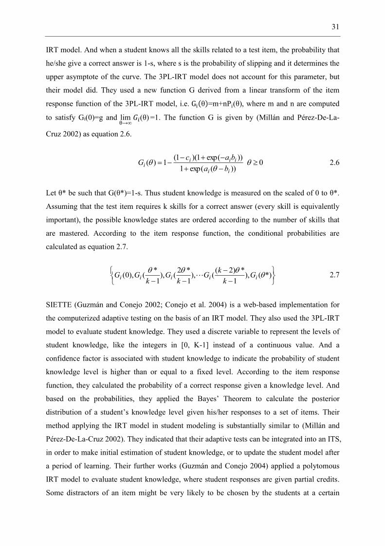
31

IRT model. And when a student knows all the skills related to a test item, the probability that

he/she give a correct answer is 1-s, where s is the probability of slipping and it determines the

upper asymptote of the curve. The 3PL-IRT model does not account for this parameter, but

their model did. They used a new function G derived from a linear transform of the item

response function of the 3PL-IRT model, i.e. Gi(θ)=m+nPi(θ), where m and n are computed

to satisfy Gi(0)=g and limθ→∞

𝐺𝑖(θ) =1. The function G is given by (Millán and Pérez-De-La-

Cruz 2002) as equation 2.6.

))(exp(1))exp(1)(1(1)(

ii

iiii ba

bacG

0 2.6

Let θ* be such that G(θ*)=1-s. Thus student knowledge is measured on the scaled of 0 to θ*.

Assuming that the test item requires k skills for a correct answer (every skill is equivalently

important), the possible knowledge states are ordered according to the number of skills that

are mastered. According to the item response function, the conditional probabilities are

calculated as equation 2.7.

*)(),

1*)2((),

1*2(),

1*(),0(

iiiii G

kkG

kG

kGG 2.7

SIETTE (Guzmán and Conejo 2002; Conejo et al. 2004) is a web-based implementation for

the computerized adaptive testing on the basis of an IRT model. They also used the 3PL-IRT

model to evaluate student knowledge. They used a discrete variable to represent the levels of

student knowledge, like the integers in [0, K-1] instead of a continuous value. And a

confidence factor is associated with student knowledge to indicate the probability of student

knowledge level is higher than or equal to a fixed level. According to the item response

function, they calculated the probability of a correct response given a knowledge level. And

based on the probabilities, they applied the Bayes’ Theorem to calculate the posterior

distribution of a student’s knowledge level given his/her responses to a set of items. Their

method applying the IRT model in student modeling is substantially similar to (Millán and

Pérez-De-La-Cruz 2002). They indicated that their adaptive tests can be integrated into an ITS,

in order to make initial estimation of student knowledge, or to update the student model after

a period of learning. Their further works (Guzmán and Conejo 2004) applied a polytomous

IRT model to evaluate student knowledge, where student responses are given partial credits.

Some distractors of an item might be very likely to be chosen by the students at a certain

32

knowledge level. In their polytomous IRT model, a characteristic curve is specified for each

choice of an item.

Johns et al. (2006) used the dichotomous IRT models for student modeling. They used EM

algorithm to learn item parameters from the data, which are collected by the Wayang Outpost,

an ITS providing tutoring on SAT mathematics problems. And they used different IRT

models, i.e. 2PL and 3PL to estimate student knowledge, and they showed the predictive

power of the models and the best result on their data is 72% accuracy to predict student

responses. Feng et al. (2009) integrated the student proficiency parameters estimated by 1PL-

IRT model into a linear regression model, which simultaneously accounts for the tutoring

assistance metrics, e.g. the number of hint requests during learning in an ITS. They used

student proficiency instead of student performance on original question, since the IRT-

estimated student proficiency takes into account the difficulty of each item. Gálvez et al.

(2013) combined an IRT model with Constraint-Based Modeling (CBM) for student modeling.

They make the constraints in CBM equivalent to the items in an IRT model, and then they

estimated the constraint characteristic curve for each constraint.

2.1.2.2 DINA and NIDA

DINA (Deterministic Input Noisy AND) (Junker and Sijtsma 2001) and NIDA (Noisy Input

Deterministic AND) (Maris 1999) are two latent variable models developed in psychometrics,

which are proposed to model the conjunctive relationship between a set of cognitive attributes

to be assessed and student performance on particular items or tasks in the assessment. They

are nonparametric models, which only require the specification of an item-by-attribute

association matrix. Since no statistical parameter estimation is required, the models can be

used on a sample size as small as 1. It can be noted that in the terminology of psychometrics,

a knowledge component or a skill is called an attribute. In the two models, both of the latent

cognitive attributes and the observations of student performance are represented by discrete

variables, thus they are also the latent class models, which aim to estimate the class

membership of a student’s knowledge. The latent classes are the complete profile of skills

which have been mastered and which have not. An accurate Q-matrix which representing the

mapping from items to attributes is required for the two models, whereas in an IRT model, the

mapping between items and a coarse-level subject is required.

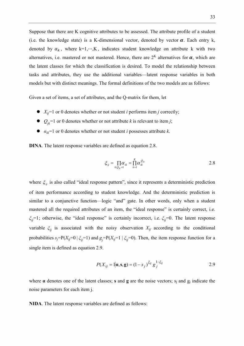
33

Suppose that there are K cognitive attributes to be assessed. The attribute profile of a student

(i.e. the knowledge state) is a K-dimensional vector, denoted by vector 𝜶. Each entry k,

denoted by 𝛼𝑘 , where k=1,⋯,K , indicates student knowledge on attribute k with two

alternatives, i.e. mastered or not mastered. Hence, there are 2K alternatives for 𝜶, which are

the latent classes for which the classification is desired. To model the relationship between

tasks and attributes, they use the additional variables—latent response variables in both

models but with distinct meanings. The formal definitions of the two models are as follows:

Given a set of items, a set of attributes, and the Q-matrix for them, let

Xij=1 or 0 denotes whether or not student i performs item j correctly;

Qjk=1 or 0 denotes whether or not attribute k is relevant to item j;

αik=1 or 0 denotes whether or not student i possesses attribute k.

DINA. The latent response variables are defined as equation 2.8.

K

k

Qik

Qkikij

jk

jk 11: 2.8

where ij is also called “ideal response pattern”, since it represents a deterministic prediction

of item performance according to student knowledge. And the deterministic prediction is

similar to a conjunctive function—logic “and” gate. In other words, only when a student

mastered all the required attributes of an item, the “ideal response” is certainly correct, i.e.

ξij=1; otherwise, the “ideal response” is certainly incorrect, i.e. ξij=0. The latent response

variable ξij is associated with the noisy observation Xij according to the conditional

probabilities sj=P(Xij=0 | ξij=1) and gj=P(Xij=1 | ξij=0). Then, the item response function for a

single item is defined as equation 2.9.

ijijjjij gsXP

1)1(),,1( gsα 2.9

where α denotes one of the latent classes; s and g are the noise vectors; sj and gj indicate the

noise parameters for each item j.

NIDA. The latent response variables are defined as follows:

34

ηijk=1 or 0 denotes whether or not student i’s performance in the context of item j is consistent

with possessing attribute k.

The latent response variable ηijk is associated with student i’s knowledge on the attribute k, i.e.

αik , according to the conditional probabilities sk=P(ηijk=0 | αik=1, Qjk=1) and gk=P(ηijk=1 |

αik=0, Qjk=1) . The observation Xij is associated with latent response variables via

Xij= ∏ ηijk= ∏ ηijkKk=1k:Qjk=1 . It is a deterministic function, which is similar to the conjunctive

function—logic “and”. Then, the item response function is defined as equation 2.10.

K

k

K

k

Qkkjkikijkij

jkikik gsQPXP1 1

1)1(),1(),,1( gsα 2.10

The DINA model associates the noise parameters with each item, i.e. sj and gj for each item j,

while the NIDA model associates the noise parameters with each attribute, i.e. sk and gk for

each attribute k. In the two models, the latent class vector 𝜶 plays the role of the latent

variable θ in IRT models, and the noise parameters sj/sk and gj/gk play the role of the item

parameters in IRT models. It should be noted that the noise parameter sj/sk and gj/gk in the

models are the error probabilities—the false negative and false positive rates. The symbols are

chosen here to be mnemonic thinking of students’ slips and guesses, but genuine slipping and

guessing behaviors may be just two possible reasons. There are many other possible reasons,

like the poor wording of the task description for students, inadequate specification of the Q-

matrix. The NIDA model is somewhat more restrictive than the DINA model, since it implies

that item response functions must be the same for all items sharing the same attributes. It

seems unrealistic that this could apply to many datasets, because it implies that item difficulty

levels would be exactly the same for many items, which is not something one expects to

observe in practice (Chiu and Douglas 2013).

2.1.2.3 Factor Analysis

The IRT models and latent class models assess a student’s knowledge from the current

performance of the student. The prior knowledge of the student used in these models might

only be the result from the last evaluation. Student historical performance and the

improvement of performance during learning are not considered in these models. But this

kind of information is also an important clue for interpreting student learning. A

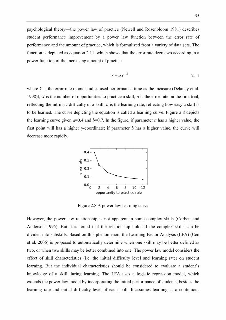
35

psychological theory—the power law of practice (Newell and Rosenbloom 1981) describes

student performance improvement by a power law function between the error rate of

performance and the amount of practice, which is formulized from a variety of data sets. The

function is depicted as equation 2.11, which shows that the error rate decreases according to a

power function of the increasing amount of practice.

baXY 2.11

where Y is the error rate (some studies used performance time as the measure (Delaney et al.

1998)); X is the number of opportunities to practice a skill; a is the error rate on the first trial,

reflecting the intrinsic difficulty of a skill; b is the learning rate, reflecting how easy a skill is

to be learned. The curve depicting the equation is called a learning curve. Figure 2.8 depicts

the learning curve given a=0.4 and b=0.7. In the figure, if parameter a has a higher value, the

first point will has a higher y-coordinate; if parameter b has a higher value, the curve will

decrease more rapidly.

Figure 2.8 A power law learning curve

However, the power law relationship is not apparent in some complex skills (Corbett and

Anderson 1995). But it is found that the relationship holds if the complex skills can be

divided into subskills. Based on this phenomenon, the Learning Factor Analysis (LFA) (Cen

et al. 2006) is proposed to automatically determine when one skill may be better defined as

two, or when two skills may be better combined into one. The power law model considers the

effect of skill characteristics (i.e. the initial difficulty level and learning rate) on student

learning. But the individual characteristics should be considered to evaluate a student’s

knowledge of a skill during learning. The LFA uses a logistic regression model, which

extends the power law model by incorporating the initial performance of students, besides the

learning rate and initial difficulty level of each skill. It assumes learning as a continuous

36

variable, and progressing gradually according to the practice frequency. It should be noted

that the learning rate is only specified for each skill in the regression model without being

individualized, in order to reduce the number of parameters. The regression model is depicted

as equation 2.12.

m

KCsjjijji

emp

nnKCsjim

11)(

)(),,( ,

2.12

where m is a logit value representing the accumulated learning for student i practicing the

knowledge components required for an item; p(m) denotes the probability of answering the

item correctly, which converts the logit value m to the prediction of observations; αi denotes

the initial knowledge of student i, i.e. the student intercept; βj denotes the easiness of

knowledge component j, i.e. the skill intercept; and the benefit of the prior practice for each

knowledge component is a function of the count n of prior practice opportunities for student i

on knowledge component j; γj is the skill slope. If giving γj as 0 and only a single βj value, this

model is equivalent to the Rasch (i.e. 1PL-IRT) model.

This regression model has a significant implication to improve the cognitive model and to

guide the instruction for each skill. For example, a skill is estimated to be mastered by a high

proportion of students. But when this skill is decomposed into two subskills, one of its

subskill might be estimated not be mastered so well by all the students. More practice should

be provided. In this case, the two subskill estimation is better than a combined skill. When a

skill has a high intercept and a low slope, and a high initial knowledge for students, less

practice on this skill should be provided to students for saving their learning time. The space

of models can be defined by domain experts to allow different possible skill levels. A

heuristic algorithm, like A* search, can be used to do model selection across the space of

models, guided by two metrics—AIC (Akaike Information Criterion) and BIC (Bayesian

Information Criterion).

The LFA model differentiates student knowledge acquisition of distinct skills. However, it is

not applicable for individualized or adaptive learning, since it ignores the correctness of

student performance at each practice opportunity. To make the model sensitive to individual

learning, Pavlik Jr et al. (2009a) modified the LFA model by introducing individual

performance, which is called the Performance Factor Analysis (PFA). The PFA model is

37

sensitive not only to the practice frequency of the skills, but also to the individual correctness

of each practice opportunity. And there are two versions of the PFA model according to

whether the difficulty parameter specified for each skill or for each item, The two versions are

called PFA-skill and PFA-item respectively (Gong and Beck 2011). The PFA model is

depicted as equation 2.13.

m

KCsjijjijjk

KCsjijjijjj

emp

itemPFAfsfsItemskKCsjimor

skillPFAfsfsKCsjim

11)(

)(),,,,(

)(),,,(

2.13

where sij and fij denote the counts of prior successes and prior failures for student i on KC j.

The parameters γj and ρj scale the effect of the observation counts on KC j. The difference is

that βj denotes the easiness of KC j, whereas βk denotes the easiness of item k. Comparing the

two versions of the PFA model, Gong and Beck (2011) found that the model with the item

difficulty parameter is slightly better on predictive accuracy than the model with the skill

difficulty parameter.

Both the PFA model and the BKT model are proposed to deal with the longitudinal

performance data collected during student learning. The two models have been compared with

each other on the predictive accuracy and parameters plausibility (Pavlik Jr et al. 2009b;

Gong et al. 2010a). They showed that the PFA model is comparable to and in some cases

better than the BKT model on predictive accuracy, and the parameters of the PFA model are

more plausible than those of the BKT model in some cases.

Some further works have investigated to improve the predictive accuracy of the PFA model.

Gong et al. (2011) improved the standard PFA by taking into account the performance order.

The intuition behind their idea is that the more recent the practice is, the more it impacts the

current problem. They introduced a decay factor to update the success and failure counts by

decreasing the weight of prior performance. To reduce the error rate of the prediction, Gong et

al. (2012) proposed to learn multiple distributions from student performance data instead of a

single distribution on overall data. They used k-means to partition students into clusters using

the confusion matrices as the feature for clustering. They used the PFA model as the basic

38

predictive model. A separated PFA model is learned for each cluster. They showed that the

multiple distribution approach improve the predictive accuracy of the PFA model. And the

multiple distribution modeling is a general idea to improve model performance. The clustered

knowledge tracing (Pardos et al. 2012a) introduced in section 2.1.1.3 is based on the same

idea, using the BKT model instead of the PFA model as the basic model. (Pavlik Jr. et al.

2011, 2015) proposed a contextual PFA model to measure learning progress of related skills

at a fine granularity. Their contextual PFA model accounts for both the individual correctness

of the prior practice and the contexts of practice. It uses the mix-effect logistic regression to

incorporate the context factors. The contextual model allows determining the best order of

practice and the appropriate amount of repetition.

2.1.3 Integrated models

Since many competing models have been proposed, Baker et al. (2011) and Pardos et al.

(2012b) examined whether the ensemble methods, which integrate multiple models, improve

predictive accuracy compared with a single model. Baker et al. (2011) integrated nine student

models (e.g. BKT and its variants, PFA) with five different ensemble methods, and compared

them with the single models. Their ensemble methods perform slightly better than the best

single model in predictive accuracy on the tutor data, but worse than the best single model on

the post-test data. Pardos et al. (2012b) implemented the similar ensemble methods. The

difference is that they integrated eight student models with eight ensemble methods. And the

ensemble methods were more effective than any single model on their data.

Two recent models integrate the IRT model with the BKT model. The Latent Factor

Knowledge Tracing (LFKT) model (Khajah et al. 2014a) associates the slip and guess

parameters with the item difficulty and the student ability. And the functions are as the

equation 2.14, where γg and γs are offsets for the slip and guess probabilities, and dj is the

difficulty of item j. Student knowledge on skill i is measured by a continuous variable, i.e. θi.

In all the prior models, the slip and guess parameters are differentiated in terms of the limited

classes. In the original BKT model, they are different over two classes, i.e. the skill is

mastered and not mastered. In the diagnostic Bayesian model (Millán and Pérez-De-La-Cruz

2002), for a item related to three skills, the two parameters are different over 23 classes. The

LFKT model individualizes the slip and guess parameters according to a continuous scale of

student knowledge. In fact, the intuition behind the LFKT model is similar to the diagnostic

Bayesian model (Millán and Pérez-De-La-Cruz 2002). Both of them attempt to use the IRT

39

distribution to specify the slip and guess parameters. However, the diagnostic Bayesian model

discretizes the student ability according to the skills. The LFKT model uses the continuous

variable to represent the student ability, and combines the IRT model with the most popular

student model—the BKT model. And they learn the IRT parameters and the transition

parameters of the BKT model simultaneously. The other more general model—Feature Aware

Student Knowledge Tracing (FAST) (González-Brenes et al. 2014) allows to individualize the

slip and guess probabilities with arbitrary features. And the model can be efficiently estimated

using a modified EM algorithm. The performance of the two models are further investigated

and compared by (Khajah et al. 2014b) and (Klingler et al. 2015).

1)(

1)(

)1(

)1(

sji

gij

dij

dij

ePs

ePg

2.14

To sum up, we compare the existing student models according to some features in principle.

The comparison shown in Table 2.2 is inspired by the presentation of the EDM conference

paper (González-Brenes et al. 2014), and involves most of the models that we have introduced

in this chapter. The models are ordered chronologically, and the recently emerging models—

LFKT and FAST incorporate all the general features of a student model.

Table 2.2 Comparison of existing models

Model allows features slip/guess ordering learning

1PL-IRT Y

Noisy-gate models/Latent class models Y

BKT Y Y Y

LFA/PFA Y Y

LFKT/FAST Y Y Y Y

2.1.4 Q-matrix

A Q-matrix is used to represent the mapping from items (observable variables) to skills (latent

variables), and also called the measurement model (Scheines et al. 2014). Most of the student

models introduced above rely on an accurate Q-matrix. A Q-matrix is usually studied by the

domain or cognitive experts. However, the human-specified Q-matrix usually contains the

subjective bias. In recent years, some researchers investigated to automatically extract the Q-

40

matrix from data. In this section, we will introduce the currently well-known approaches of

extracting the Q-matrix from data.

Barnes et al. (2005) proposed a method to extract an optimal Q-matrix from student response

data. Their method evaluates the fit of a Q-matrix to data by calculating the total error using

the Q-matrix. The total error is the sum of the errors over all data records. For each data

record, the error is the Hamming distance between the nearest ideal response vector and the

observation vector. To find an optimal Q-matrix, they used a heuristic hill climbing method

which varies Q-matrix values to minimize the fitting error. Their Q-matrix method has better

error rates on fourteen experimental data sets than factor analysis, but has worse error rates

than k-means cluster analysis. Barnes (2005) studied the effectiveness of the Q-matrix method

in understanding and directing student learning. The extracted Q-matrix and the expert

defined Q-matrix differ, but student responses are understandable based on extracted Q-

matrix. They also found that the Q-matrix method often predicts the same questions for

further review as those the self-guided students chose for themselves. And students who chose

differently from the Q-matrix method could have benefited from reviewing a Q-matrix

selected concept.

Beheshti and Desmarais (2012) used the Matrix Factorization technique to extract Q-matrix

and to assess student skills mastery from student performance data. They tried to improve the

matrix factorization algorithm by employing the partial order constraints that are derived with

the POKS algorithm from the same data. (Desmarais et al. 2012; Desmarais and Naceur 2013)

extended a technique based on Non-negative Matrix Factorization to construct the conjunctive

item to skill mapping from test data. They used simulated student test data to validate their

approach and their results show that their approach yields reliable mapping for items

involving one or two skills from a set of six skills. Beheshti et al. (2012) applied two

techniques, namely the Singular Value Decomposition (SVD) and a wrapper approach, to

determine the number of dominant latent skills. Desmarais et al. (2014) discussed three

techniques to refine the Q-matrix.

2.2 Skill Models

A skill model referred here only involves the hidden layers in the graph of “learner modeling

layers” in (Desmarais and Baker 2012). We will introduce the issues of interest for the skill

models, and the prevalent methods to deal with these issues.

41

2.2.1 Granularity

Granularity hierarchy is a common representation of a student model. It describes how a

domain is decomposed into components (Millán et al. 2010). Knowledge components in a

domain model are commonly described at different grained levels. A granularity hierarchy

captures different levels of details in a type of semantic network. Aggregation relationships

are used to describe the relationships between knowledge components at different grained

levels. Aggregation relationships can be used to split a composite knowledge component into

multiple knowledge components at a finer-grain size. The observers are usually related to

knowledge components at the finest-grained level. The observed information is propagated

through the aggregation links to knowledge components at the coarser-grained levels. The

AND-OR clustering scheme are proposed by Collins et al. (1996) to capture the aggregation

relationships and the equivalent groups in their granularity hierarchy.

Figure 2.9 Two alternatives to model aggregation relationships (Millán et al. 2000)

Millán et al. (2000) and Millán and Pérez-De-La-Cruz (2002) measured student knowledge at

three levels of granularity, that is, concepts, topics and subjects. They analyzed two

alternatives (see Figure 2.9) to model the aggregation relationships between knowledge

components at two different levels of granularity, where knowledge component KC can be

divided in a finite set of finer knowledge components KC1,⋯,KCn . In alternative 1, the

structure means that KC1,⋯,KCn are mutually independent a priori. Regarding the probability

propagation, positive evidence of mastering KCi increases the probability of mastering KC,

and positive evidence of mastering KC increases the probability of mastering every KCi. In

alternative 2, the structure means that KC1,⋯,KCn are mutually independent given KC.

Positive evidence of mastering KCi increases the probability of mastering KC, which in turn

increases the probability of every other KCi, and positive evidence of mastering KC increases

the probability of every KCi. Alternative 1 implies the fact that students learn in an

incremental way. That is, in order to learn about a topic, a student must learn all the concepts

42

that form part of it. The underlying assumption in alternative 2 is the same with IRT models:

there is a single value that explains a student’s behavior. Assuming binary nodes, knowing

KC means every part of it known. They chose alternative 1 in their model. To quantitatively

represent the aggregation relationships in a BN, they proposed the following law to assign the

condition probabilities:

Condition distribution of node T given the corresponding concepts C1,⋯,Cn, is defined

as equation 2.14.

1:

1 ),,1(iCi

in wCCTP 2.15

Condition distribution of node A given the corresponding topics T1,⋯,Tm, is defined

as equation 2.15.

1:

1 ),,1(jTj

jmTTAP 2.16

where iw and j are the normalized weight vector that measures the relative importance of

each concept in a topic or each topic in a subject to which it belongs.

Tchétagni and Nkambou (2002) proposed to assess student knowledge on propositional logic

at several levels of granularity. They used the alternative 2 model in Figure 2.9 to represent

aggregation relationships in their hierarchy. They pointed out that in this architecture there are

restrictions on the way evidence propagates throughout the network. This is due to the fact

that two child nodes may influence their parent, without influencing each other: they are d-

separate. Carmona and Conejo (2004) used the alternative 1 model to represent the

aggregation relationships in their learner model used in MEDEA, an open system to develop

ITSs. Some recent approaches discussed the granularity of skill model in the perspective of

statistics. Skill models in these approaches only involve the finest-grained knowledge

components, which directly explain student behaviors. A standing issue in a student model is

at what level of granularity student skills should be modeled. Pardos et al. (2007) explored the

models with varying levels of skill granularity (1, 5, 39, and 106 skill models) and measure

the accuracy of these models by predicting student performance within their ITS, i.e.

ASSISTment, as well as in a state standardized test. Their results showed that the finer the

granularity of the skill model, the better the prediction of student performance.

43

2.2.2 Prerequisite Relationships

Prerequisite relationships commonly exist among the knowledge components of some

domains. Reye (2004) analyzed how to use Bayesian networks to model prerequisite

relationships. They stated that the conditional probabilities in a Bayesian network should meet

some conditions. For example, if knowledge component A is a prerequisite of knowledge

component B, equation 2.17 should be satisfied. However, they also stated the prerequisite

relationship is not always strict, so they allow the uncertainty for the conditional probabilities.

The uncertainty values for these conditional probabilities are specified by experts in their

method.

0))(_)(_(

1))(_)(_(

AknowsstudentBknowsstudentP

BknowsstudentAknowsstudentP 2.17

Carmona et al. (2005) introduced the prerequisite relationships to a generic BN student model

for MEDEA, in order to improve the efficiency of both adaptation mechanisms and the

inference process. They used a modified noisy AND-gate or a modified noisy OR-gate to

model the prerequisite relationships. Ferguson et al. (2006) used EM algorithm to learn the

hidden parameters in BNs and compared the flat skill model (the skills are mutually

independent) with hierarchical skill model (prerequisite relationships between skills given a

priori) according to Bayesian Information Criterion (BIC). Their results show that a

hierarchical model better fits their data than the flat model does.

Figure 2.10 A Bayesian network modeling aggregation and prerequisite relationships

simultaneously

Millán et al. (2010) discussed a problem which commonly arises in student modeling, that is,

to simultaneously model prerequisite and granularity relationships. If both are included in the

44

same model, links with different interpretations are mixed, and then it is difficult to build and

understand the model. For example, if a composite skill KC which is composed of two sub-

skills, KC1 and KC2, and there is also a skill P which is a prerequisite of KC. The conditional

probabilities of K given its parents are difficult to be specified (Figure 2.10 (a)). They

suggested a solution which is to group variables of the same type by introducing intermediate

variables (Figure 2.10 (b)).

45

Chapter 3: Towards Improving Evidence Model

We have reviewed the student modeling techniques in chapter 2 according to the two parts of

a student model—the evidence model and the skill model. We also attempt to improve the

two parts of a student model. In this chapter, we introduce our work towards improving the

evidence model, while in the next chapter we introduce our work towards improving the skill

models. The two parts of a student model are improved for providing a better foundation for

individualized learning.

Various kinds of information can be obtained during student learning. We refer to the

information as the features in this thesis. The most commonly used feature is the correctness

of student behaviors. Most of the existing models are proposed to use this feature. However,

the correctness simply categorizes student behaviors into two groups, that is, the correct ones

and the incorrect ones. Many diagnostic features during student learning are ignored by

existing models. In this chapter, we attempt to improve the accuracy of the evidence models

by making use of the diagnostic features.

The organization of this chapter is as follows. In section 3.1, we introduce the common

diagnostic features which can be obtained during learning. We also discuss the existing

methods which incorporate these diagnostic features. In section 3.2, we introduce two well-

known conjunctive models to deal with the noise in student behaviors. The two conjunctive

models are the latent class models. We propose a general graphical model which can be

equivalent to the latent class models. In section 3.3, we extend the graphical model which is

equivalent to the NIDA model to incorporate the diagnostic feature—student erroneous

responses. We evaluate our model on knowledge estimation and performance prediction using

a set of metrics. We compare our model with other two diagnostic models. Moreover, the

three diagnostic models are compared with the binary models to verify whether the diagnostic

feature improves the accuracy of student models. In section 3.4, we compare the performance

of two common student models. And we investigate the potential relationship between the

two parameters in the two models. A possible direction for future work is discussed. In

section 3.5, we summarize our work towards improving evidence model. Our work in this

chapter have been published in the proceedings of the ITS conference (Chen, Wuillemin and

Labat 2014).

46

3.1 Diagnostic Features

Most of existing models only deal with the student response data characterized by a common

feature—correctness. Student responses are categorized into two groups, that is, correct and

incorrect. This categorization is too simply and coarse-grained, and much information in

students’ behaviors are ignored. Some features can be obtained during student learning and

can be used for the more precise categorization of student behaviors.

One important feature is the error pattern. Student erroneous responses are informative, which

might be caused by different types of knowledge bias or lack. This feature is usually

overlooked by the binary models. If we can recognize student error patterns, and associate

each error pattern with the corresponding type of knowledge bias or lack, student behaviors

can be more precisely recognized. A psychometric model—MC-DINA proposed by De La

Torre (2009) is an extension of the DINA model, which transfers student responses to

multiple choice items to their knowledge states. In their MC-DINA model, the erroneous

responses are the distractors which are coded to associate with the types of knowledge lack.

The knowledge lack used in this thesis indicates that some required skills are not mastered.

For example, if a correct response requires three skills, it can be coded as 111. And if a

distractor is coded as 101, students who choose this distractor are very likely to lack the

second skill. The polytomous response data are used, and thereby the variables representing

observations are multinomial rather than binary. The binary DINA model has been introduced

in section 2.1.2.2. Compared with the binary DINA model, the observed variable Xij in

equation 2.9 is a multinomial variable in the MC-DINA model, whose values are the options.

The latent response variable ξij is also multinomial, and whose values denote the groups of

ideal response patterns. Each of the coded options including the correct response and

distractors is a group. All the remaining ideal response patterns which do not correspond to

any distractor are in one group. In their MC-DINA model, the noise parameters are used to

represent the conditional probabilities between two multinomial variables, i.e. P(Xij | ξij). The

MC-DINA model distinguishes student behaviors in multiple groups. Student erroneous

behaviors are recognized by the MC-DINA model.

Besides the error pattern, other important features are the item difficulty and student ability.

Most of existing models do not distinguish items and student abilities. For example, in the

binary NIDA model and the original BKT model, items related to the same set of skills have

47

the same response functions. The item 3+2 is considered to be equivalent with the item 12+7

in these models. In the binary DINA model and the original BKT model, the novice and

medium students have the same probability to guess the correct answer. The IRT model

(which has been introduced in section 2.1.2.1) uses a statistic scaling method to characterize

items with the feature—item difficulty and to characterize student abilities. To my

knowledge, the initial research to introduce the item difficulty and student ability into a

graphical model is the paper of Millán and Pérez-De-La-Cruz (2002), which has been

introduced in section 2.1.2.1. Their diagnostic model combines the IRT model with a

conjunctive dynamic Bayesian network model. The item difficulty parameter for each item is

learned by the IRT model. And student knowledge corresponding to an item is discretized

into several ordinal categories. The slip and guess parameters for each item are specified by

the IRT model with the discrete ability values and the item difficulty value. Although they

still used the binary response data, they applied an IRT distribution to model the probabilities

of a correct response given different types of knowledge lack. Their model distinguishes

different types of knowledge lack. However, their model has not been empirically evaluated.

And in their dynamic Bayesian network, there is no transition parameter, which is different

from the BKT model.

In recent researches, the item difficulty has been introduced into the most popular student

model—the BKT model. All the parameters in the original BKT model are skill-specific, that

is, the parameters are learned per skill. The KT-IDEM model (Pardos and Heffernan 2011)

introduced the item difficulty into the BKT model. Instead of measuring the item difficulty,

like the IRT model, they learned the item-specific slip and guessing parameters, that is, the

slip and guess parameters are fitted for each item. The LFKT model proposed by Khajah et al.

(2014a) integrates the IRT model into the BKT model. In their model, the slip and guess

parameters are individualized by the item difficulty and student ability. FAST (González-

Brenes et al. 2014) provides a general framework to individualize the slip and guess

parameters with arbitrary features. Given student and problem features, FAST discovers the

weights equivalent to student ability and the item difficulty.

In student learning with an ITS, some features besides the correctness, like the number of

attempts, the number of hints and the response time also provided information about student

knowledge. Wang and Heffernan (2013) used a partial credit method to introduce these

features into the BKT model. They measured student behaviors with a continuous variable,

48

and proposed an award and penalty algorithm to score student behaviors. The prediction

accuracy of the BKT model is improved by using the partial credit values. In this chapter, we

attempt to improve the accuracy of the evidence model by introducing the diagnostic

feature—error patterns.

3.2 A General Graphical Model

In many educational scenarios, a correct response to a problem step or a task requires multiple

skills. And uncertainty exists in transferring student performance to knowledge. To deal with

the two issues simultaneously, some probabilistic conjunctive models have been proposed. At

present, the well-known models are the DINA model and the NIDA model. It should be

noticed that the original BKT model is not a conjunctive model, where each observation is

only related to one skill. Its variant is proposed to model multiple subskills (Xu and Mostow

2012). In this section, we focus on the DINA model and the NIDA model.

The DINA and NIDA model are the latent class models, which have been introduced in

section 2.1.2.2. They can deal with the uncertainty in student modeling. And they are also

conjunctive models, which can represent the relationship between an item and the multiple

related skills. Although the models are described in different theoretical frameworks and

terms, the latent class models are substantially similar to some Bayesian network models. The

graphical models which are equivalent to the DINA and NIDA models are depicted in Figure

3.1. We use a general framework to describe these graphical models. There are three levels of

nodes in the models corresponding to the variables used in the latent class models. One level

involves the attribute (i.e. skill) nodes; the second level involves the nodes representing the

latent response variables; the third level involves the observation nodes. An attribute node

describes student knowledge of an attribute. An observation node denotes student

performance to an item. Latent response variable nodes are the auxiliary nodes. In the DINA

and NIDA models, all the nodes are binary. The structure of the three levels of nodes can be

described by the internal structure of an ICI (independence of causal influence) model (Díez

and Druzdzel 2006).

According to Figure 3.1, the DINA model is equivalent to a simple “AND” model (Díez and

Druzdzel 2006). In the simple “AND” model, there is only one latent response node, which

represents the ideal response in the DINA model. The conditional function between the

attributes nodes and the latent response node is the logic “AND” gate. That is, only when all

49

the attribute nodes are in the state of 1, the latent response node is in the state of 1; otherwise,

the latent response node is in the state of 0. In the simple “AND” model, the conditional

probabilities of the observation node given the states of the latent response node are specified

by two noise parameters—the slip and guess parameters. That is, Psj=P(Xj=0 | ξj=1) and

Pgj=P(Xj=1 | ξj=0). According to Figure 3.1, the NIDA model is equivalent to the noisy-AND

model (see section 2.1.1.1). In the noisy-AND model, the parents have the independent

influence to the child. That is, the distributions of the attribute nodes affect the distribution of

the observation node independently. In the noisy-AND model, each attribute node is related to

one latent response node. And the conditional probabilities of a latent response variable node

given the states of the linked attribute node are specified by a pair of noise parameters—the

slip and guess parameters. That is, Psi=P(ηji=0 | αi=1) and Pgi=P(ηji=1 | αi=0). In the noisy-

AND model, the conditional function between the latent response nodes and the observation

node is logic “AND” gate.

Figure 3.1 A general graphical conjunctive model

According to the equivalent graphical models, the slip and guess parameters are specified for

each item in the DINA model, whereas they are specified for each skill in the NIDA model.

Please note that the original NIDA model assume the noise parameters for each skill in

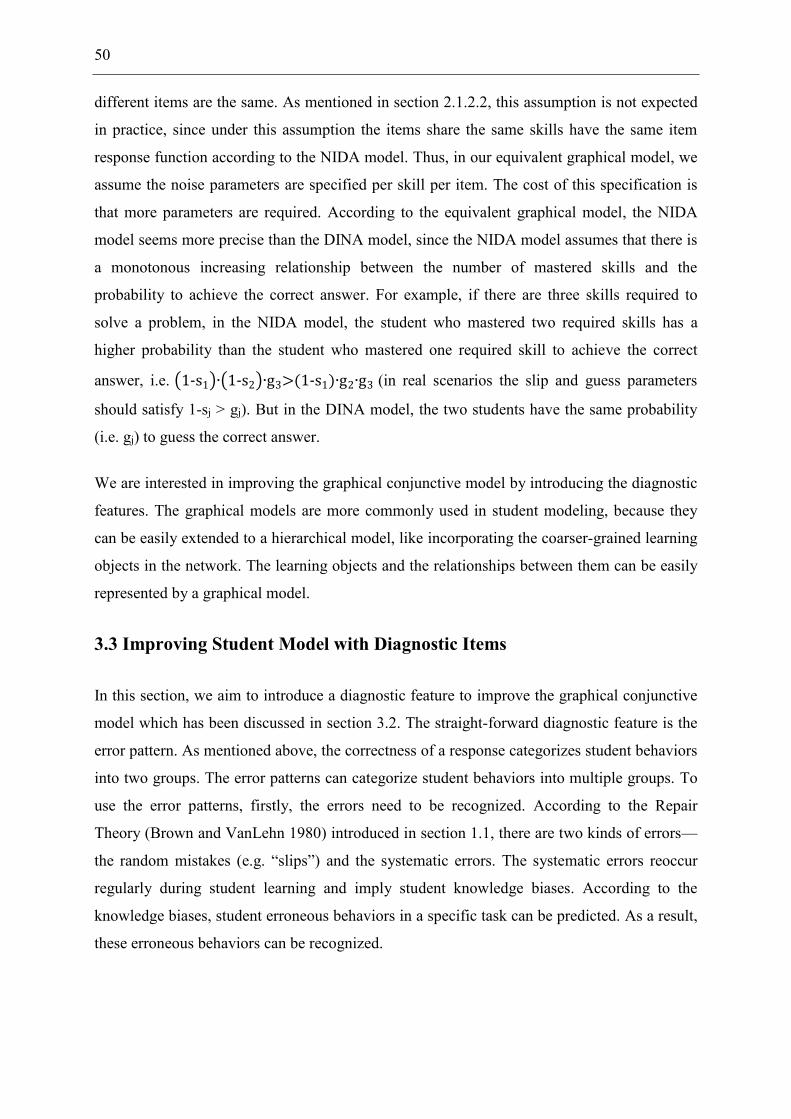
50

different items are the same. As mentioned in section 2.1.2.2, this assumption is not expected

in practice, since under this assumption the items share the same skills have the same item

response function according to the NIDA model. Thus, in our equivalent graphical model, we

assume the noise parameters are specified per skill per item. The cost of this specification is

that more parameters are required. According to the equivalent graphical model, the NIDA

model seems more precise than the DINA model, since the NIDA model assumes that there is

a monotonous increasing relationship between the number of mastered skills and the

probability to achieve the correct answer. For example, if there are three skills required to

solve a problem, in the NIDA model, the student who mastered two required skills has a

higher probability than the student who mastered one required skill to achieve the correct

answer, i.e. (1-s1)∙(1-s2)∙g3>(1-s1)∙g2∙g3 (in real scenarios the slip and guess parameters

should satisfy 1-sj > gj). But in the DINA model, the two students have the same probability

(i.e. gj) to guess the correct answer.

We are interested in improving the graphical conjunctive model by introducing the diagnostic

features. The graphical models are more commonly used in student modeling, because they

can be easily extended to a hierarchical model, like incorporating the coarser-grained learning

objects in the network. The learning objects and the relationships between them can be easily

represented by a graphical model.

3.3 Improving Student Model with Diagnostic Items

In this section, we aim to introduce a diagnostic feature to improve the graphical conjunctive

model which has been discussed in section 3.2. The straight-forward diagnostic feature is the

error pattern. As mentioned above, the correctness of a response categorizes student behaviors

into two groups. The error patterns can categorize student behaviors into multiple groups. To

use the error patterns, firstly, the errors need to be recognized. According to the Repair

Theory (Brown and VanLehn 1980) introduced in section 1.1, there are two kinds of errors—

the random mistakes (e.g. “slips”) and the systematic errors. The systematic errors reoccur

regularly during student learning and imply student knowledge biases. According to the

knowledge biases, student erroneous behaviors in a specific task can be predicted. As a result,

these erroneous behaviors can be recognized.

51

Recognizing student systematic errors requires a large amount of knowledge engineering

effort. The general procedure is that: firstly, for each learning task or item, the common errors

should be collected; then the errors should be analyzed by experts, and the patterns of the

errors should be extracted; finally, the mapping from each error pattern to the knowledge bias

should be constructed. For example, to the fraction addition item 2 3⁄ + 1 8⁄ , a common

erroneous response is 3 11⁄ . The error pattern can be described as “adding/subtracting both

the numerators and denominators”, which corresponds to the knowledge bias of “believing

that fractions’ numerators and denominators can be treated as separate whole numbers”.

Students with the knowledge biases need to repair their current knowledge on the skill of

“adding fractions with unlike denominators”. And to a multi-skill item, student error patterns

might be caused by the knowledge bias or lack on different skills. For example, to the item 3-

5*4, a common erroneous response is -8, which is caused by the knowledge bias on the skill

“following the order of operations”. Another common erroneous response is 17, which is

caused by the knowledge bias on the skill “subtraction”. To a multi-skill item, some erroneous

responses are not “fully” wrong. Besides the skills with knowledge biases, some other skills

might be correctly used. For example, students who give the erroneous response 17 still

correctly “follow the order of operations” and “multiplication”.

Recognizing student error patterns is a tough and time-consuming task, especially for the

open-ended problems. The amount of student erroneous responses to open-ended items can be

infinite. And it is also difficult to find the causes for the various errors. Multiple choice

questions are a common type of items to assess student knowledge. The multiple choice items

restrict a student’s response to be one of its options, which make it easier to recognize student

erroneous behaviors. Moreover, some distractors can be designed by experts to be the

common errors, and at the same time, the types of knowledge bias or lack can be associated

with the distractors. Hence, analyzing student responses to multiple choice items is an easy

way to recognize student erroneous behaviors. In this section, we target on analyzing student

response data to the multiple choice items. We extend the graphical conjunctive model

introduced in section 3.2 to model student behaviors including the erroneous responses. We

evaluate whether the diagnostic feature—error pattern improves the accuracy of the evidence

model by comparing the diagnostic model with the original (binary) model. We also compare

our diagnostic model with other diagnostic models. A simulated data set and a real data set

are used for the evaluation.

52

3.3.1 A Diagnostic Model

To analyze student responses to a multi-skill item using the conjunctive graphical model, an

accurate Q-matrix is required. To interpret the error patterns of an item, the mapping from the

errors to the knowledge biases is also required. Thus, for a multiple choice item, the Q-matrix

should indicate the mapping from the correct option to the required skills, and the mapping

from the distractors to the types of knowledge lack. To represent these mappings, we use the

binary codes for the correct options and the distractors. For a multiple choice item, a binary

model use the correctness feature to identify student behaviors, that is, correct option (1) and

the other options (0). In our diagnostic model, for a multiple choice item requiring three skills,

the correct option is coded as 111. And the distractors are also coded in the same way. For

example, a distractor coded as 101 indicates the second skill is incorrectly used. Figure 3.2

shows an example of multiple choice items with coded options. When an option is not

identified, it is coded as x. According to the options, student behaviors are categorized into

multiple groups. And each group is associated with the latent knowledge state. It should be

noted that in this thesis, we are interested in which skill the student has a bias, instead of the

knowledge bias itself, i.e. the misconception. In fact, if the misconceptions are defined, they

can be easily incorporated in a graphical model. In this thesis, we focus on diagnosing the

skills that students have biases according to their erroneous responses.

Figure 3.2 A multiple choice item with coded options

The probabilistic graphical models provide the sound formulism to deal with the uncertainty

in inferring student knowledge from performance. Although, these models are initially

proposed for the dichotomous data, they can be extended for the polytomous data without

modifying the model topology, just by replacing the binary nodes with the multinomial nodes.

For a general Bayesian network conjunctive model, to incorporate the erroneous behaviors,

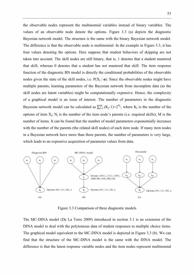
53

the observable nodes represent the multinomial variables instead of binary variables. The

values of an observable node denote the options. Figure 3.3 (a) depicts the diagnostic

Bayesian network model. The structure is the same with the binary Bayesian network model.

The difference is that the observable node is multinomial. In the example in Figure 3.3, it has

four values denoting the options. Here suppose that student behaviors of skipping are not

taken into account. The skill nodes are still binary, that is, 1 denotes that a student mastered

that skill, whereas 0 denotes that a student has not mastered that skill. The item response

function of the diagnostic BN model is directly the conditional probabilities of the observable

nodes given the state of the skill nodes, i.e. P(Xj | α). Since the observable nodes might have

multiple parents, learning parameters of the Bayesian network from incomplete data (as the

skill nodes are latent variables) might be computationally expensive. Hence, the complexity

of a graphical model is an issue of interest. The number of parameters in the diagnostic

Bayesian network model can be calculated as ∑ (Kj-1)×2NjMj=1 , where Kj is the number of the

options of item Xj; Nj is the number of the item node’s parents (i.e. required skills); M is the

number of items. It can be found that the number of model parameters exponentially increases

with the number of the parents (the related skill nodes) of each item node. If many item nodes

in a Bayesian network have more than three parents, the number of parameters is very large,

which leads to an expensive acquisition of parameter values from data.

Figure 3.3 Comparison of three diagnostic models

The MC-DINA model (De La Torre 2009) introduced in section 3.1 is an extension of the

DINA model to deal with the polytomous data of student responses to multiple choice items.

The graphical model equivalent to the MC-DINA model is depicted in Figure 3.3 (b). We can

find that the structure of the MC-DINA model is the same with the DINA model. The

difference is that the latent response variable nodes and the item nodes represent multinomial

54

variables. Likewise, the values of an item node denote its options. In the MC-DINA model,

the ideal responses denoted by ξj are categorized into several groups, where the correct

response is a group as well as every distractor is a group, and all the other ideal responses are

in one group. Each group is an alternative value for the latent response variable ξj. The item

response function of the MC-DINA model is as equation 3.1. Since both the item nodes and

the latent response variable nodes are multinomial, the number of the noise parameters for

each item is increased compared with the binary DINA model (which only has two

parameters). The number of the parameters (conditional probabilities here) in the MC-DINA

model can be calculated as ∑ (Kj-1)×(Kj*+1)M

j=1 , where M is the number of items; Kj is the

number of the options of item Xj; Kj* is the number of the coded options (incorporating the

correct option and the distractors) for item Xj. Here we use Kj* instead of Kj, since some

erroneous options cannot be interpreted and the reason cannot be recognized. The number of

the parameters in the MC-DINA model does not increase with the number of the parents of

each item, and instead it is only related to the number of the options and the coded options.

Thus compared with the diagnostic Bayesian network model, the number of parameters in the

MC-DINA model is reduced, especially for the item nodes with multiple parents. In the

example shown in Figure 3.3, the number of the parameters in the diagnostic BN model is 27,

whereas in the MC-DINA model it is 15. It can be noticed that the number of parameters for

the root nodes is also added.

)()( jjj XPXP α 3.1

However, the MC-DINA model treats equivalently the knowledge states which do not

correspond to any coded option. For example, students with knowledge state 000 and students

with knowledge state 110 are considered to select the four options with the same probability

distribution. As mentioned in section 3.2, the NIDA model assumes that the probability of

giving a correct response is an accumulative function of the number of skills mastered. To

differentiate all the knowledge states, we propose a diagnostic model which is an extension of

the NIDA model. The graphical description of our model is shown in Figure 3.3 (c). The

structure of our model is the same with the graphical model equivalent to the NIDA model.

Similarly, the item nodes are multinomial variables, with the values denoting the options. The

skill nodes and the latent response variable nodes are binary. The values of the latent response

variables ηji can be interpreted as the correctness of the related skills used in the items, that is,

1 denotes that a skill is correctly used, while 0 denotes that a skill is incorrectly used. The

55

latent response variables in our model are called the used skills in this thesis. The noise

parameters between the skill nodes and the latent response nodes are specified per skill per

item, that is, the slip and guess parameters as equation 3.2.

jiiji

jiiji

PgP

PsP

)01(

)10(

3.2

In our model, the conditional probabilities of an item node given the states of the latent

response variable nodes can be specified in two ways. One is absolutely deterministic, and the

other is partially deterministic. The two ways of the specification for the conditional

probabilities P(Xj=Ok | ηj1, ηj2, ηj3) are shown in Table 3.1. When a student correctly uses all

the relevant concepts for answering a question, his/her answer is certainly the right option.

When some concepts are not correctly used by the student, his/her answer is certainly the

coded wrong option which corresponds to his/her performance. When the student's

performance does not correspond to any coded option of the questions, he/she might select

any of the options. In the deterministic specification, the joint states of the used skills which

do not correspond to the correct answer or any distractor are supposed as the behaviors

unrecognized. They are associated with the erroneous options without codes. If all the options

of an item are coded (i.e. each option is either a correct option or a distractor), we suppose an

additional option which is associated with other alternative states of used skills. Using the

deterministic specification, the number of parameters is largely reduced. The number of

conditional parameters in our model is 2× ∑ NjMj=1 , where M is the number of items and Nj is

the number of skills required for a correct response to item Xj.

Table 3.1 Two ways of the specification for conditional probabilities

Used skills (ηj1, ηj2, ηj3)

deterministic partially deterministic

O1 (011)

O2 (111)

O3 (101)

O4 (x)

O1 (011)

O2 (111)

O3 (101)

O4 (x)

000 0 0 0 1 0.25 0.25 0.25 0.25

... ... ...

011 1 0 0 0 1 0 0 0

100 0 0 0 1 0.25 0.25 0.25 0.25

... ... ...

111 0 1 0 0 0 1 0 0

56

In the partially deterministic specification, when the states of the used skills do not

correspond to any coded option, we suppose that any option can be selected. We assign noise

parameters to each option given one of these states of the used skills. The initial value to the

noise parameters are the same, that is, 0.25 for each of the four options. These noise

parameters can be learned from data. In this specification, the number of conditional

parameters to be estimated is ∑ (2×NjMj=1 +(Kj-1)×(2Nj-𝐷𝑗)), where M is the number of items;

Nj is the number of the skills required for a correct response to item Xj; Kj is the number of

the options of item Xj; Dj is the number of coded options. As a result, using the deterministic

specification, our model only requires 9 parameters in the example of Figure 3.3, while using

the partially deterministic specification, our model requires 24 parameters. Compared with the

other two models, in this example, our model with the deterministic specification requires the

least parameters. Compared with the diagnostic BN model, both our model and the MC-

DINA model reduce the number of parameters. The item response function of our model is as

equation 3.3, where α is the skill vector; αi denotes one entry; Nj is the number of the skills

required a correct response to item Xj; fj(x)=P(Xj=Ok | ηj1, ηj2, ηj3) (see Table 3.1).

jii

N

ijijijj gsxfXP

1

)1()1)(()( α 3.3

In this section, we have introduced our diagnostic model—a modified NIDA model to

interpret student erroneous behaviors. We also introduce the diagnostic Bayesian network

model—a general Bayesian network model modified to incorporate student erroneous

behaviors. Additionally, we also introduce the MC-DINA model—a modified DINA model to

interpret student errors. We have compared the three diagnostic models in principle. In

section 3.3.3, we will evaluate our diagnostic model as well as the other two diagnostic

models. We will compare the three models using a simulated data set and a real data set.

Before that, we will introduce the common metrics for evaluating student models.

3.3.2 Metrics for Student Model Evaluation

Many different metrics are used to evaluate and compare the performance of student models.

A good choice of metrics is important for the comparison of student models. The common

metrics for the evaluation of student models have been discusses by Pelánek (2015). We will

introduce some metrics which can be used to evaluate the models discussed in this thesis.

57

Confusion Table Metrics. Confusion Table is widely used and underlies a set of metrics for

analyzing the correctness of a classification model (Pardos and Yudelson 2013). Table 3.2 is

an example for the binary classification. TP refers to the count of the positive cases that are

correctly predicted. The other three values (i.e. TN, FP, FN) have their corresponding

meanings. If there are n classes, the confusion table is a table of size n by n. If the prediction

is not categorical, like a probability in [0, 1], it is customary to round it. That is, probabilities

of 0.5 and greater become 1; those less than 0.5 become 0. The common metrics based on the

confusion table are described by equations 3.4a-3.4d. F-measure is a combination of the

precision and recall.

Table 3.2 Confusion Table

Actual

Correct Incorrect

Predicted Correct True Positive (TP) False Positive (FP)

Incorrect False Negative (FN) True Negative (TN)

FNFPTNTPTNTPaccuracy

3.4a

FPTPTPprecision

3.4b

FNTPTPrecall

3.4c

recallprecisonrecallprecisionmeasureF

2 3.4d

Metrics Based on Log-likelihood. The likelihood function describes how likely the data are

observed given the parameters of a model. Since the likelihood tends to be an incredibly small

number, so it is generally easier to work with the logarithm of the likelihood. The log-

likelihood of a sample of data given the parameters of a model is calculated as equation 3.5a,

where n is the sample size; oi is the observations (actual class) and pi is the predictions.

Besides the log-likelihood itself, there are several metrics which are based on the log-

likelihood. AIC (Akaike Information Criterion) and BIC (Bayesian Information Criterion) are

most commonly used for student models. These metrics penalize the number of model

parameters and the number of data points in order to avoid overfitting. The AIC value of a

58

model is computed as equation 3.5b, while the BIC value is computed as equation 3.5c, where

the k is the number of model parameters and N is the number of data points. For the log

likelihood, the higher value is better. For the AIC and BIC, the lower value is better.

ni iiii popoLL

1)1ln()1()ln( 3.5a

kLLAIC 22 3.5b

)ln(2 NkLLBIC 3.5c

RSME (Root Mean Square Error) is a common error metric for the evaluation of student

models. It accounts for the squared differences between the predictions and the observations,

which is depicted as equation 3.6, where n is the sample size; oi is an observation (actual class)

and pi is a prediction. In educational data mining, especially for the evaluation of skill mastery

models (e.g. the BKT models), the RSME metric is commonly used, though the resulting

numbers is hard to interpret in the context of student modeling. For the RSME, the lower

value is better.

ni ii po

nRSME

12)(1 3.6

The log-likelihood and RSME are the metrics of probabilistic understanding of the errors

(Pelánek 2015), both of which has the form of “sum of penalties for individual errors”. The

confusion table metrics are based on qualitative understanding of errors, either the prediction

is correct or incorrect. Various metrics for the evaluation of student models have been

investigated by Pardos and Yudelson (2013). They found that the three confusion table

metrics—recall, F-measure and accuracy are the best metrics for predicting the moment of

learning (i.e. knowledge estimation). And the RMSE and likelihood based metrics are the best

metrics to recover the ground truth parameters. The models discussed in this thesis are

evaluated by one or several of these metrics.

3.3.3 Evaluation

In this section, we evaluate our model using a simulated data (or called synthetic data) set and

a real data set. We explain how we generate the simulated data, and the basic information of

the real data. Using the two data sets, we evaluate our diagnostic model as well as the other

59

two models (i.e. the diagnostic Bayesian network model and the MC-DINA model (De La

Torre 2009)) based on a set of metrics. We compare the performance of the three diagnostic

models. Moreover, we evaluate the binary models which have the same graphical structures

with the three diagnostic models using the same data sets. We compare the diagnostic models

with the binary models, in order to verify whether the introduced error patterns can improve

the accuracy of student models.

3.3.3.1 Data Sets

A simulated data set. It is difficult to know the real distribution of the responses to the

multiple choice items for students with different knowledge states. To make the simulated

data more comparable to the real data, we generate the data based on the diagnostic Bayesian

network model using the parameter values from the real data set. This data generation method

is also used by Beheshti and Desmarais (2015). We use the general Bayesian network

structure instead of the other two models, since the other two models simplify the noisy

parameters under some assumptions. We implement the Bayesian network model via the

Bayes Nets Toolbox (BNT) (Murphy 2001), which is an open-source Matlab package for

directed graphical models. This package is widely used in the applications of probabilistic

graphical models, since it supports many kinds of nodes (i.e. variables with different

probability distributions, such as multinomial nodes, multinomial logit nodes, Gaussian nodes

etc.), static and dynamic BNs, many different exact and approximate inference algorithms,

parameters and structure learning. We generate the data of 1000 students with a Bayesian

network model, which contains 20 item nodes and 5 skill nodes. Each item requires two or

three skills for a correct response. In the Bayesian network, the skill nodes are the binary

variables, i.e. mastered and not mastered. Please note that the values of a binary variable are

denoted as 1 (false) and 2 (true) in the BNT package. The prior probability for each skill node

is given as 0.5. The items are the four-option questions, each of which contains a correct

option and one or two distractors coded to indicate the skills lacked. The item nodes are the

multinomial variables with four discrete values representing the options. For each multiple

choice item, the Q-matrix is required to incorporate the mapping from the correct option to

the skills, as well as the mapping from the distractors to the skills. As mentioned above, to

make the simulated data more comparable to the real data, the mapping of each item to the

skills is selected from the real data. And the conditional parameters for each item are specified

by the parameter values which are estimated from the real data introduced below. According

60

to the specified Bayesian network, we randomly generate student response data. The function

“sample_bnet” in the BNT package can be used. And for each simulated student, the

knowledge state is generated simultaneously with the response data according to the Bayesian

network.

A real data set. A real data set about student response data to multiple choice items is

available via the R package CDM (Robitzsch et al. 2014). The data set named “data.cdm01”

is used in our experiment, which incorporates the response data of 5003 students on 17

multiple choice items. Three skills are assessed in the data set. The Q-matrix is made by

experts, which indicates the mapping from correct option and distractors to skills. Please note

that the options which are neither the correct option nor the distractors are coded as 000 in the

Q-matrix. There are eight items related to one skill and other eight items related to two skills

and one item related to three skills. Among the items, nine of them contain four options and

others contain two options. Among the items with four options, two items have no coded

distractors, that is, the options are coded correct or incorrect; one item has two correct options.

Since our diagnostic model targets on assessing student knowledge on the multiple choice

items with one or more distractors, student response data on six of the items are select for our

experiment. The selected items, i.e. {I1, I2, I3, I6, I7, I8}, have four options, among which

there is one or more coded distractors, and only one correct option. And only one item is

related to three skills, all the other items are related to the first two skills.

3.3.3.2 Comparison of Three Diagnostic Models

We evaluate our diagnostic model as well as other two diagnostic models with a set of metrics,

and compare the performance of them. Since the differences among the three models are the

model complexity (the number of parameters) and the assumptions of the noise assigned for

observations, we should evaluate the fit of the three models to the data. Moreover, to account

for the model complexity, we compare the AIC and BIC values of the three models. The three

models are proposed to diagnose student knowledge, thus we also evaluate the prediction

accuracy of the three models. We use the commonly used metrics—RSME and accuracy

(based on confusion table) for evaluating and comparing the three models.

Bayesian network construction. We implement all the three models in the paradigm of

Bayesian networks. And the Bayesian networks are constructed by using the BNT package

(Murphy 2001). The R package CDM (Robitzsch et al. 2014) also provides a function named

61

“mcdina” to implement the MC-DINA model in the paradigm of latent variable models. In

our experiments, we use the BNT package to implement the MC-DINA model as a graphical

model. The Bayesian network for each of the three models is constructed according to Figure

3.3 and the given Q-matrix. For the simulated data, the Q-matrix is predetermined; for the real

data, it is made by human experts. In our model and the MC-DINA model, besides the skill

and item nodes, the related latent response variable nodes are added in the networks. In our

model, for each skill, a binary latent response variable node is added. In the MC-DINA

model, for each item, a multinomial latent response variable node is added.

Parameters initialization. Before learning the parameters from data, we have to initialize the

parameters. In the diagnostic BN model, if the joint state of the skill nodes corresponds to a

coded option, the probability of selecting that coded option is initialized to 0.85 and other

three options with a probability of 0.05 respectively. If the joint skill state does not

correspond to any coded option, the probability for every option is initialized with the equal

value, i.e. 0.25. In the MC-DINA model, as mentioned above, the conditional function

between the skill nodes and the latent response variable nodes is logic “AND”, i.e.

deterministic. The noise parameters between a latent response variable node and an item node

have to be initialized. The latent response variable node and the item node are the multinomial

nodes. The values of the latent response variable node denote the groups of the ideal

responses. The values of the item node are the same with the other two models and denote the

options. When the group of the latent response variable node corresponds to an option, the

probability for that option is initialized to 0.85, and other three options are initialized to a

probability of 0.05. When the group does not correspond to any option, all the options are

initialized to an equal probability, i.e. 0.25. In our model, the slip and guess parameters

between the skill nodes and the latent response nodes are initialized to be 0.1 and 0.2. As

discussed above, the conditional parameters of the item nodes given the values of latent

response nodes can be specified in two ways—deterministically and the partially

deterministically. Using the deterministic specification, no additional noise parameter needs

to be specified. Using the partially deterministic specification, the conditional probabilities

are initialized with the same value (i.e. 0.25) given the joint states of the latent response

variable nodes which do not correspond to any coded option. We implement our diagnostic

model using the two parameter specifications.

62

Parameters Learning. Since there are some latent nodes (i.e. the skill nodes and the latent

response variable nodes) in each Bayesian network, the parameters are learned from the

incomplete data. The commonly used algorithm to learn the parameters of a Bayesian network

from incomplete data is the Expectation Maximization (EM) algorithm (Dempster et al. 1977;

Borman 2009), which is introduced in section 2.1.1.1. The BNT package provides a function

named “learn_params_em” for directly implementing the EM algorithm to learn the

parameters from incomplete data. This function requires three input arguments—the Bayesian

network with initialized parameters, the data table and the iteration conditions. We set the

maximum number of the iterations is 50 and the minimum variance of the likelihood is

0.0001. The EM algorithm learns the parameter values which maximize the likelihood of data.

Results—Model fit and complexity. To compare the fit to data and the complexity of the

three diagnostic models, we input the whole data set (both in the simulated data experiment

and in the real data experiment) for the EM algorithm to learn the parameters of the best fit.

The resulting maximum log-likelihood for each of the three models is shown in Table 3.3.

The maximum log-likelihood of a model demonstrates the fit of the model to data. The higher

the maximum log-likelihood, the better the model fits data. According to Table 3.3, for both

the data sets, the diagnostic BN model fits best. Our model using the partially deterministic

specification fits the simulated data better than the MC-DINA model, while the opposite

result is got on the real data. Using the partially deterministic specification, our model fits

both the simulated data and the real data much better than using the deterministic

specification.

As mentioned above, one of the differences among the three diagnostic models is the model

complexity. Thus we also compare the number of parameters the three models. And the

formulas to calculate the number of parameters for each model have been provided in section

3.3.1. The resulting number of parameters for each model in the experiments using the

simulated data and using the real data is shown in Table 3.3. We can find that our model using

the deterministic specification needs the least parameters. Our model using the partially

deterministic specification requires more parameters than the MC-DINA model in the

simulated data, but requires less parameter in the real data, since there are more nodes with

three parents in the simulated data. According to the formulas in section 3.3.1, our model

using partially deterministic specification will requires more parameters than the MC-DINA

model if there are many item nodes with three or more parents.

63

Table 3.3 The performance of the three diagnostic models on two data sets

Diagnostic BN

MC-DINA Our model (deterministic)

Our model (partially deterministic)

Simulated data

Log-likelihood -21991 -22421 -24056 -22384

Number of parameters

485 293 105 377

AIC 44952 45428 48322 45522

BIC 48785 47744 49152 48502

Real data

Log-likelihood -34584 -34604 -35784 -35058

Number of parameters

87 63 35 47

AIC 69342 69334 71638 70210

BIC 70065 69858 71929 70610

As discussed in section 3.3.2, the AIC and BIC metrics make a trade-off between the model

fit and the model complexity by rewarding log-likelihood and penalizing the number of

parameters and the number of data points. Thus, we also compare the AIC and BIC values of

the three models. We calculate the AIC and BIC values for each model according to the

equations 3.5b and 3.5c. The resulting AIC and BIC values for each model is shown in Table

3.3. As mention above, the lower the AIC or BIC value is, the better the model is. According

to Table 3.3, the MC-DINA model has the best AIC and BIC values in the real data, and the

best BIC values in the simulated data. The diagnostic BN model has the best AIC value in the

simulated data. Although our model using the partially deterministic specification fits better

than the MC-DINA model, it requires more parameters. As a result, our model has a relatively

worse AIC and BIC values. If many items in data related to three or more skills, the model

complexity should be taken into account. Thus the AIC or BIC metrics should be used for

selecting models. In our experiments, according to the AIC and BIC values, the MC-DINA

model is preferred among the three models.

64

Besides the model fit and complexity, we are also interested to compare the prediction

accuracy of the three diagnostic models. The prediction accuracy of a student model involves

the percentage of correctly forecasting student knowledge or student future performance.

Since student knowledge is latent and cannot be observed, the knowledge estimation is

usually replaced by the performance prediction. Fortunately, we use a simulated data set,

where the knowledge states of each student is known beforehand. Thus, in the experiment

using the simulated data, we evaluate both the accuracy of knowledge estimation and

performance prediction of the three models.

K-fold cross-validation. To evaluate the prediction accuracy, we have to partition the data

into the training data and the testing data. We can simply divide a data set into two subsets,

like 70% of data as the training data and 30% of data as the testing data. This method is called

the holdout method. However, the evaluation using this data partitioning method can have a

high variance. The evaluation results may heavily rely on which data points are for training

and which for testing. K-fold cross-validation is one way to reduce the variance. In the k-fold

cross-validation (Kohavi 1995; Han et al. 2011), the initial data are randomly partitioned into

k mutually exclusive “folds” (i.e. subsets), each of approximately equal size. And the training

and testing are performed for k times. For each iteration, one fold is used for testing, and the

remaining k-1 folds are used to train the model. Thus, all the data points are used for both

training and testing, and each data point is used for testing exactly once. The accuracy of the

model is computed based on all the predictions in the k iterations.

Results—prediction accuracy. We use 10-fold cross-validation to estimate the prediction

accuracy of the three diagnostic models. In our experiment, the real data are partitioned into

10 subsets at student level. That is, in each iteration, the data of 90% of students are used for

training and 10% are used for testing. It should be distinguished from the data partition at

item level. That is, the data on 90% items are used for training and 10% for testing. The

model parameters are learned from the training data by using the EM algorithm. After the

parameters of the model are learned, we predict student performance in the testing data.

For the simulated data, we evaluate two kinds of predictions—the knowledge estimation and

the performance prediction. For the real data, since the real knowledge state of a student

cannot be known, we only evaluate the performance prediction. In the knowledge estimation,

using the learned parameters, we estimate the knowledge state of each student in the testing

data given student response data. We input the response record of a student in the testing data

65

as the evidence in the Bayesian network. Then the inference engine will propagate the

information backward through the Bayesian network to the skill nodes. The posterior

probabilities of the skill nodes are calculated. These probabilities are rounded. That is, when

the posterior probability of a skill node is higher than 0.5, we suppose the skill is mastered by

the student; otherwise, the skill is not mastered by the student. In this way, the knowledge

state of each student is predicted. We compare the predicted knowledge state of each student

with the actual knowledge state in the simulated data. The four counts (i.e. TP, TN, FP, FN)

in the confusion table can be obtained. According to equation 3.4a, the accuracy can be

computed.

In the performance prediction, for each student record in testing data, all the observations

except one are given as the evidence to the Bayesian network. That is, the observation of one

item node is unseen. And a student’s response to the unseen item will be predicted by the

models. The process of predicting a student’s response to an unseen item is as follows: when

the evidence is given to the model, the Bayesian network inference algorithm (the junction

tree engine is used via the BNT package) estimates student knowledge on each skill as well as

predicts the probability distribution of student performance on the unseen item node. Since

each of our diagnostic items (i.e. a multiple choice item) has four options, the predicted

probability distribution incorporates the probabilities for the four options. In other words,

there are four classes for prediction. In our experiment, the option with the highest probability

is considered as the response of the student. For example, if the predicted probability

distribution of the hidden item is {0.03, 0.17, 0.68, 0.12}, the student’s response is supposed

to be the third option. Each item is iteratively selected as the unseen item, and a student’s

response to the unseen item is predicted. This process is similar to the leave-one-out cross-

validation. The leave-one-out cross-validation is a special case of the k-fold cross-validation,

where k is the size of the initial data. Here, k is the number of item nodes. It is not the real

cross-validation, since the “training” data (the observations except the hidden one) are used as

the evidence in the Bayesian network instead of training parameters.

Since the performance is a multinomial variable, the prediction is a multi-class prediction.

Thereby in our experiments, the confusion table is a 4×4 matrix. Comparing the predictions

with the observations in the testing data, the counts in the confusion table can be obtained.

And the accuracy values of the models can be calculated by an equation similar to equation

3.4a. To calculate the RSME value of multi-class prediction, we use a binary code to

66

represent the performance. For example, if the response is predicted to be the third response,

the prediction is represented as 0010. Accordingly, observations are coded in the same way.

As a result, the difference between a prediction and an observation can be calculated as the

half of the Hamming distance. In our experiments, we predict two kinds of student

performance. We predict which option is selected by a student (i.e. multinomial prediction),

as well as whether the student response’s is correct or not (i.e. binary prediction).We evaluate

the two kinds of performance prediction of the three models using both the simulated data and

the real data. The knowledge estimation is only implemented for the simulated data.

Table 3.4 Prediction accuracy of the three diagnostic models on two data sets

Diagnostic BN

MC-DINA Our model (deterministic)

Our model (partially deterministic)

Simulated data

Accuracy (knowledge estimation)

0.9564 0.9534 0.9022 0.9522

Accuracy (multinomial)

0.5988 0.5906 0.5612 0.5924

Accuracy (binary)

0.8780 0.8744 0.8577 0.8760

RSME (knowledge estimation)

0.2088 0.2159 0.3127 0.2186

RSME (multinomial)

0.6334 0.6398 0.6625 0.6385

RSME (binary)

0.3492 0.3543 0.3773 0.3522

Real data

Accuracy (multinomial)

0.5800 0.5799 0.5515 0.5654

Accuracy (binary)

0.8449 0.8446 0.8346 0.8451

RSME (multinomial)

0.6481 0.6482 0.6697 0.6592

RSME (binary)

0.3938 0.3942 0.4067 0.3936

We insist to use the accuracy metric since the values are interpretable for a student model. We

also use the most commonly used error metric—RSME which has been introduced in section

3.3.2. The resulting accuracy and RSME values of the three models on the simulated data and

the real data are shown in Table 3.4. It can be found that the accuracy and the RSME values

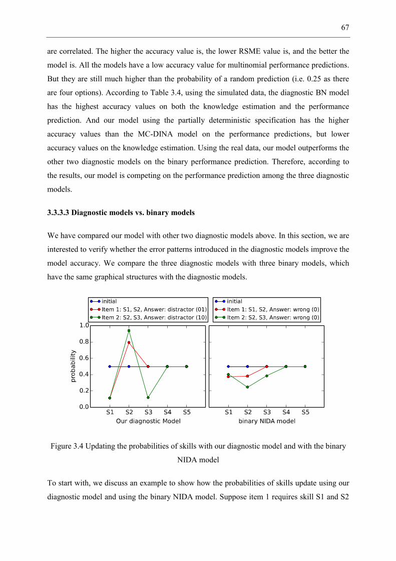
67

are correlated. The higher the accuracy value is, the lower RSME value is, and the better the

model is. All the models have a low accuracy value for multinomial performance predictions.

But they are still much higher than the probability of a random prediction (i.e. 0.25 as there

are four options). According to Table 3.4, using the simulated data, the diagnostic BN model

has the highest accuracy values on both the knowledge estimation and the performance

prediction. And our model using the partially deterministic specification has the higher

accuracy values than the MC-DINA model on the performance predictions, but lower

accuracy values on the knowledge estimation. Using the real data, our model outperforms the

other two diagnostic models on the binary performance prediction. Therefore, according to

the results, our model is competing on the performance prediction among the three diagnostic

models.

3.3.3.3 Diagnostic models vs. binary models

We have compared our model with other two diagnostic models above. In this section, we are

interested to verify whether the error patterns introduced in the diagnostic models improve the

model accuracy. We compare the three diagnostic models with three binary models, which

have the same graphical structures with the diagnostic models.

Figure 3.4 Updating the probabilities of skills with our diagnostic model and with the binary

NIDA model

To start with, we discuss an example to show how the probabilities of skills update using our

diagnostic model and using the binary NIDA model. Suppose item 1 requires skill S1 and S2

68

for a correct response, and item 2 requires S2 and S3. The observations on each item are

erroneous options. The observations are identified as the distractors in our diagnostic model,

while in the binary NIDA model they are measured as wrong answers. Figure 3.4 shows the

probabilities of skills updated given the observations one by one. The parameter values

learned from the real data are used. To learn the parameters of a binary NIDA model, we need

to convert the polytomous data to the binary data, that is, the correct option is denoted as 1

and all the other options are denoted as 0. It should be noted that the noise parameters in the

binary NIDA model in this experiment are learned per skill per item, like our diagnostic

model. It is different from the original NIDA model, whose noise parameters are learned per

skill. In this example, for the sake of comparison, the probability of each skill is initialized as

0.5 instead of using the learned parameters. According to Figure 3.4, when a student selects a

distractor which is coded as 01, our diagnostic model increases the probability of skill S2 and

decreases that of S1, whereas the binary model identifies the distractor as wrong, and decrease

the probabilities of both the skills. Given an observation on item 2, the two models perform in

the same way. According to the updating process of skill probabilities, it seems that our

diagnostic model more precisely distinguishes student behaviors, which might lead to the

better estimation of student knowledge.

The binary models used for the comparison are the binary BN model, the binary DINA model

and the binary NIDA model. We use the 4-fold cross validation to evaluate the prediction

accuracy of the three binary models. As mentioned above, the polytomous data should be

transformed into the binary data. That is, the correct option is coded as 1 and the other three

options are coded as 0. In these experiments, the partially deterministic specification is used

for our model. In the binary DINA model, the latent response variable nodes are binary. The

noise parameters between the latent response nodes and an item node are a pair of the slip and

guess parameters. These experiments are also implemented via the BNT package (Murphy

2001). The Bayesian networks for the binary models are unchanged from the diagnostic

models. Only the item nodes and the latent response variable nodes become binary variables

accordingly. The parameters are learned from the training data by the EM algorithm. Using

the learned parameters, student knowledge and student performance on unseen items can be

predicted. Comparing the predictions with observations, the accuracy and RSME values of

knowledge estimation and performance prediction for each model can be calculated. Since in

the binary models, the item nodes are binary, all the performance predictions of these models

are binary (i.e. whether a student’s response is correct or incorrect).

69

The resulting RSME values of the three diagnostic models and the three binary models using

the simulated data and the real data are shown in Figure 3.5. In both the knowledge estimation

and the performance prediction, the diagnostic models have better RSME values than the

binary models on the simulated data and the real data. Therefore, the error patterns improve

the accuracy of student models. In addition, we see that the RSME values of the diagnostic

models are significantly lower than those of the binary models on the knowledge estimation,

but slightly lower on the performance prediction. The interval values in each figure indicate

the smallest and largest RSME improvement values. Using the simulated data, compared with

the binary models, the largest RSME improvement of the diagnostic models on the knowledge

estimation is 0.1793 and the smallest is 0.1653. The largest RSME improvement of the

diagnostic models on the performance prediction is roughly 0.0197 and the smallest is

roughly 0.0139. And using the real data, the RSME improvement values of the diagnostic

models are between 0.0037 and 0.0044. The small improvements on the performance

prediction might be caused by the high probability of guessing for the multiple choice items.

Figure 3.5 Diagnostic models vs. binary models

We are also interested in how the prediction accuracy changes given an increasing number of

observations. We estimate the accuracy of the knowledge estimation by giving different

number of observations. The accuracy values of the diagnostic models and the binary models

are shown in Figure 3.6. The three diagnostic models have a significantly higher accuracy

values than the binary models given any number of observations. The observations selected

for every model are the same at each time. And the prediction accuracy of the diagnostic

models increases more sharply than the binary models with the increasing number of

70

observations. This demonstrates that the diagnostic items are more discriminative than the

binary items for classifying student knowledge. The result is reasonable, since the coded

distractors of the diagnostic items distinguish student behaviors more precisely. Therefore, the

diagnostic models outperform the binary models. And the performances of the three

diagnostic models are closed to each other, while the performances of the three binary models

are also close to each other.

Figure 3.6 Diagnostic models vs. binary models with different number of observations

3.4 Comparison of Existing Models

Various student models have been proposed in different paradigms. These student models

have the complementary strengths and weaknesses. The latent class models—DINA and

NIDA which have been used in section 3.3 are proposed to infer student knowledge on fine-

grained skills from their performance on multi-skill tasks. And these models rely on an

accurate Q-matrix, which indicates the mapping from tasks to fine-grained skills. The Item

Response Theory (IRT, the latent trait model) model (see more details in section 2.1.2.1)

addresses individual differences among students and items. The Q-matrix is not required for

the IRT model, and instead each task is only labeled by the topic which it involves. The

popular student model—the BKT model (see more details in section 2.1.1.3) tracks student

knowledge during learning, and in the original BKT model, each observation is only labeled

by one skill (or knowledge component). The latent class models and the BKT model make no

distinction among students and problems (Khajah et al. 2014a). The latent class models and

the IRT model ignore student knowledge transitioning during learning. The IRT model

measures student overall ability on a topic, and it cannot indicate student knowledge on a

71

fine-grained skill, which might result in the failure of providing informative feedback to

students. The original BKT model cannot estimate student knowledge on the subskills.

In recent years, a trend to improve student modeling is to integrate the features used in

different student models into one student model. A variant of the BKT model (Xu and

Mostow 2011) traces student knowledge on multiple subskills. The recent research (Khajah et

al. 2014a) integrates the IRT model with the BKT model. And (González-Brenes et al. 2014)

proposed a general framework to integrate the arbitrary features into the BKT model. In this

section, we compare the performance of two models—the DINA model and the IRT model,

and especially we analyze the features used in the two models, and the potential relationships

between them.

At the starting point, we analyze and compare the DINA model and the IRT model. We

evaluate the two models using two real data sets named “data.ecpe” and “data.fraction1” in

the CDM package (Robitzsch et al. 2014). The ECPE data incorporate the responses of 2922

students to 28 items, while the Fraction data incorporate 536 students’ responses to 15 items.

In both the data sets, the response data are binary, 1 (correct) and 0 (incorrect). We use the 4-

fold cross-validation to evaluate the prediction accuracy of the two models. We implement the

commonly used Rasch (1PL-IRT) model in our experiment. That is, each item is only

characterized by the difficulty, and the discrimination and guess parameters are restricted to

be constants, i.e. 1 and 0 respectively. Student ability is measured by a continuous variable θ,

and the probability of student j with the ability θj giving a correct response to item Qi with

difficulty bi can be computed as equation 3.6.

1)( )1()1( ij b

ji eQP 3.6

The Rasch model is implemented via the R package ‘ltm’ (Rizopoulos 2006). This package is

developed for the analysis of dichotomous and polytomous data using latent trait models,

including the Rasch model, 2PL model, 3PL model, etc. The function named “rasch” in the

package is used to fit the model to data. The two arguments of this function are the training

data and a constraint to specify the discrimination parameter for each item with 1. The

difficulty parameter for each item is learned by this function. Using the learned parameters,

we can evaluate the accuracy of predicting student performance on unseen items. For each test

record, all of the observations except one are given as evidence to the model with the learned

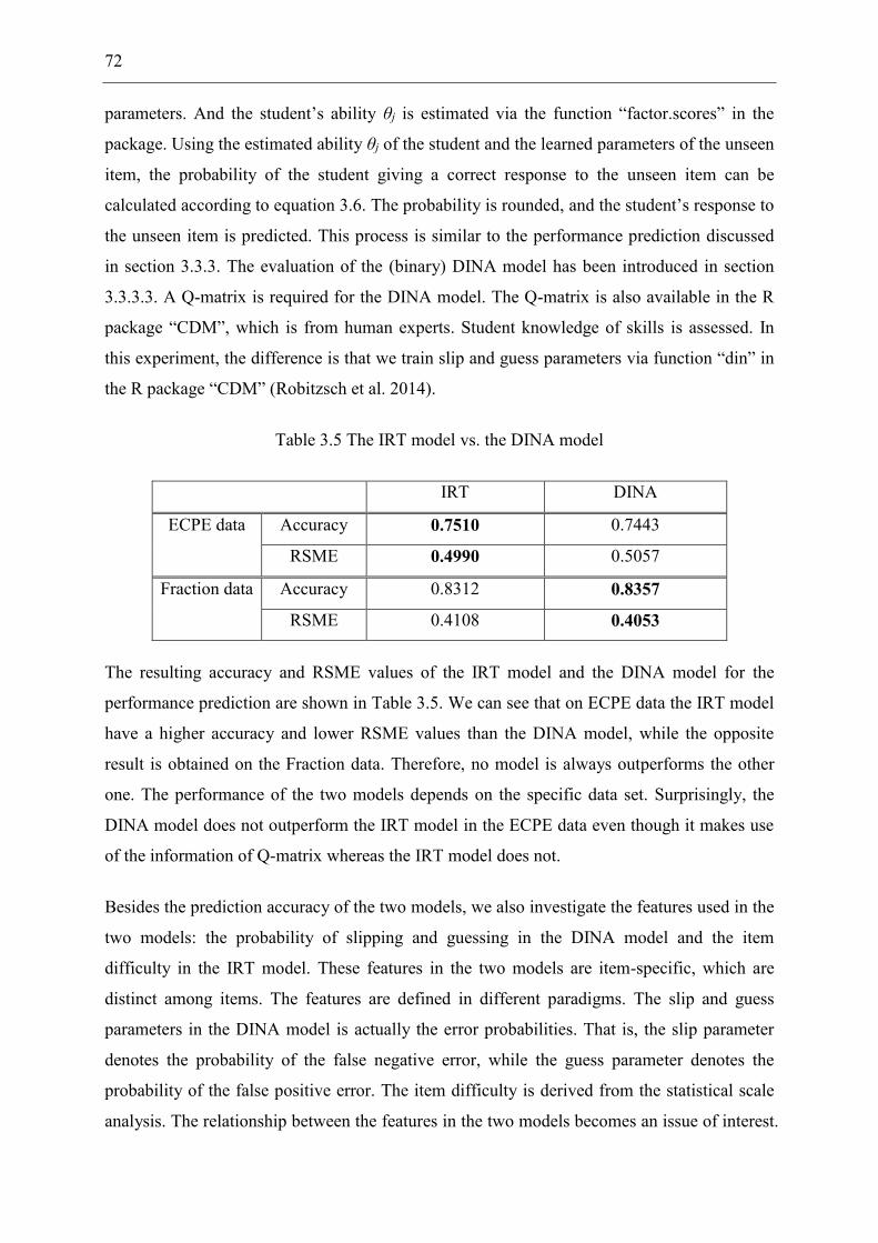
72

parameters. And the student’s ability θj is estimated via the function “factor.scores” in the

package. Using the estimated ability θj of the student and the learned parameters of the unseen

item, the probability of the student giving a correct response to the unseen item can be

calculated according to equation 3.6. The probability is rounded, and the student’s response to

the unseen item is predicted. This process is similar to the performance prediction discussed

in section 3.3.3. The evaluation of the (binary) DINA model has been introduced in section

3.3.3.3. A Q-matrix is required for the DINA model. The Q-matrix is also available in the R

package “CDM”, which is from human experts. Student knowledge of skills is assessed. In

this experiment, the difference is that we train slip and guess parameters via function “din” in

the R package “CDM” (Robitzsch et al. 2014).

Table 3.5 The IRT model vs. the DINA model

IRT DINA

ECPE data Accuracy 0.7510 0.7443

RSME 0.4990 0.5057

Fraction data Accuracy 0.8312 0.8357

RSME 0.4108 0.4053

The resulting accuracy and RSME values of the IRT model and the DINA model for the

performance prediction are shown in Table 3.5. We can see that on ECPE data the IRT model

have a higher accuracy and lower RSME values than the DINA model, while the opposite

result is obtained on the Fraction data. Therefore, no model is always outperforms the other

one. The performance of the two models depends on the specific data set. Surprisingly, the

DINA model does not outperform the IRT model in the ECPE data even though it makes use

of the information of Q-matrix whereas the IRT model does not.

Besides the prediction accuracy of the two models, we also investigate the features used in the

two models: the probability of slipping and guessing in the DINA model and the item

difficulty in the IRT model. These features in the two models are item-specific, which are

distinct among items. The features are defined in different paradigms. The slip and guess

parameters in the DINA model is actually the error probabilities. That is, the slip parameter

denotes the probability of the false negative error, while the guess parameter denotes the

probability of the false positive error. The item difficulty is derived from the statistical scale

analysis. The relationship between the features in the two models becomes an issue of interest.

73

Intuitively, if an item is more difficult, it seems that students are more likely to slip and less

likely to guess.

We still use the real data set “data.ecpe” (i.e. ECPE data) via the R package “CDM”

(Robitzsch et al. 2014) to investigate the relationship between the parameters of the DINA

model and the difficulty parameter of the IRT model. We use the whole data set to train the

parameters of the DINA model. Likewise, the parameters of the DINA model are learned via

the “din” function in the package. Using the same data set, we train the parameters of the

Rasch model via the “ltm” package. After the slip/guess parameters and item difficulty are

learned by the two models respectively, we investigate the relationship between the guess and

item difficulty parameters as well as the relationship between slip and difficulty parameter

respectively. We plot each item in the data set using the probability of guessing and its

difficulty value as the coordinates in Figure 3.6 (left). Each item is also plotted with the

probability of slipping and its difficulty value as the coordinates in Figure 3.6 (right).

Figure 3.6 Probabilities of guessing and slipping varying with the difficulty values

According to Figure 3.6, it is plausible that the probability of guessing monotonically

decreases with the difficulty value, and the probability of slipping value monotonically

increases with the difficulty value. In fact, the paper of Khajah et al. (2014a) at the EDM

(Educational Data Mining) conference stated that the probability of slipping and guessing for

an item satisfy a logistic regression function of the item difficulty and student ability. This

paper has been discussed in section 2.1.3 and the logistic regression function is described as

equation 2.14, which is the integration of the BKT model and the IRT model (called the

LFKT model). To verify this logistic regression function between the parameters, we

calculate the log odds of the slipping and guessing as equation 3.7. The log odds of an event

74

A are logit(P(A))=ln(P(A)/P(┐A)). Then equation 2.14 can be transformed as equation 3.7.

That is, the log odds of slipping and guessing are a linear function of the item difficulty.

sijij

ijij

gjiij

ijij

dPs

PsPs

dPg

PgPg

1ln)logit(

1ln)logit(

3.7

We look into whether there is a linear relationship between the log odds logit(Pgij)/logit(Psij)

and the item difficulty dj. We calculate the log odds of guessing and slipping, i.e. logit(Pgij)

and logit(Psij), for each item in terms of the slip and guess parameter values. And we plot

each item using the log odds and its difficulty value as the coordinates in Figure 3.7.

According to this figure, all the points seem to follow a line with a slope of 1 or -1 (the

dashed lines). Thus the log odds of guessing and slipping are likely to follow the linear

function of the item difficulty. And the log odds of guessing linearly decrease with the

increasing difficulty values, while the log odds of the slipping linearly increase with the

increasing difficulty values. The result looks consistent with the equation 3.7, i.e. the findings

of the LFKT model (Khajah et al. 2014a).

Figure 3.7 Log odds of guessing and slipping varying with different difficulty values

The LFKT model is an integrated model of the IRT model and the BKT model. It

individualizes the slip and guess parameters in the BKT model with the item difficulty and

student ability as equation 3.7. However, the original BKT model cannot estimate student

knowledge on multiple subskills. The DINA model deals with student behaviors to multi-skill

tasks. The slip and guess parameters in the DINA probably can be individualized based on

75

item difficulty and student ability. In this thesis, we only present our preliminary work on

analyzing the features in the two models. Integrating the features to improve student modeling

can be further studied.

3.5 Summary

In this chapter, we present our work towards improving diagnostic ability of the evidence

model. Most evidence models focus on dealing with the binary data, that is, student behaviors

are measured as right or wrong. To a multi-skill item, student erroneous responses might be

caused by the knowledge lack of different skills. We introduce the diagnostic items—multiple

choice questions to recognize student erroneous responses. The distractors of the multiple

choice items are labeled with the corresponding type of knowledge lack. Thereby, student

behaviors are categorized into multiple groups. We extend a latent class model—the NIDA

model to deal with the uncertainty in transferring the polytomous performance data to student

knowledge. We use a simulated data set and a real data set to evaluate our diagnostic model

with a set of metrics. And we compare our model with other two diagnostic models—the

diagnostic BN model and MC-DINA model (De La Torre 2009). The results demonstrate that

our model is competing on the performance prediction among the three models. We also

compare the three diagnostic models with the binary models, which have the same graphical

structures with the diagnostic models. The results show that the accuracy of student models is

improved by introducing error patterns of student responses. In addition, we compare the

prediction accuracy of two popular evidence models—the DINA model and the IRT model

using two real data sets. And we present our preliminary work on analyzing the relationships

between the probability of guessing/slipping in the DINA model and the item difficulty in the

IRT model.

76

77

Chapter 4: Towards Improving Skill Model

Human knowledge acquisition usually complies with some characteristics or laws. Learning

sequence is an important characteristic inherent in student learning. Student learning begins

with basic concepts and simple tasks, and move to more complex concepts and challenging

tasks. Learning sequence is supported by the psychological theory of the zone of proximal

development (Vygotsky 1980). Students should be given the experiences that are within their

zones of proximal development, thereby encouraging and advancing their individual learning.

This theory stratifies the learning objectives. In the sequence perspective, some skills should

be learned before others. The learning sequence is usually expressed by the prerequisite

relationships between problems and between skills. Prerequisite structures of fine-grained

skills are the basis for designing individual learning sequence.

In this chapter, we attempt to improve the skill model by incorporating prerequisite structures

of skills, and we focus on learning skill structures from student performance data. In section

4.1, we discuss the prerequisite relationships in student models, and introduce the related

work on extracting prerequisite structures from student response data. In section 4.2, we

present our two-phase method to discover prerequisite structures of skills from data. In

section 4.3, we evaluate our method using the simulated data and the real data. In section 4.4,

we compare our method with the other two methods. In section 4.5, we verify whether the

accuracy of a student model is improved by introducing the prerequisite structure of skills.

Section 4.6 is a summary of this chapter.

4.1 Prerequisite Relationships

Prerequisite relationships between problems and skills have been investigated by many

educators and researchers. The prerequisite structures express the latent cognitive order.

Students should be capable of solving the easier problems before the difficult ones are

presented to them, and likewise, some preliminary skills should be learned prior to the

learning of the complex skills. The prerequisite relationships underlie the strategies for

individualized learning. Furthermore, improving the accuracy of a student model with the

prerequisite structure of skills has been exemplified by Chen et al. (2014) and Käser et al.

(2014). We introduced the prerequisite relationships of skills into a student model (Chen et al.

2014). The results of our experiments (which will be discussed in section 4.5) show that the

78

model accuracy is improved. Prerequisite relationships have also been introduced into the

BKT model (Käser et al. 2014). Their experiments on five real data sets demonstrate that the

predictive accuracy of the BKT model is significantly improved.

The prerequisite structures of problems and skills are in accordance with Knowledge Space

Theory (Falmagne et al. 2006) and Competence-based Knowledge Space Theory (Heller et al.

2006). A student’s knowledge state should comply with the prerequisite structure of skills. If

a skill is mastered by a student, all the prerequisites of the skill should also be mastered by the

student. If any prerequisite of a skill is not mastered by a student, it seems difficult for the

student to learn the skill. Therefore, according to the knowledge states of students, we can

uncover the prerequisite structure of skills. Most prerequisite structures of skills reported in

the student modeling literature are studied by domain or cognition experts. It is a tough and

time-consuming task since it is quite likely that the prerequisite structures from different

experts on the same set of skills are difficult to come to an agreement. Moreover, the

prerequisite structures from domain experts are seldom tested empirically. Nowadays, some

prevalent data mining and machine learning techniques have been applied in cognition models,

benefiting from large educational data available from online educational systems. Deriving

the prerequisite structures of observable variables (e.g. problems) from data has been

investigated by some researchers. However, discovering prerequisite structures of skills is still

challenging since a student’s knowledge of a skill is a latent variable. Uncertainty exists in

inferring student knowledge of skills from performance data. Our work aims to discover the

prerequisite structures of skills from student performance data.

With the emerging educational data mining techniques, many works have investigated the

discovery of prerequisite structures within domain models from data. One of the most famous

approaches is the Partial Order Knowledge Structures (POKS) learning algorithm, which is

proposed by Desmarais and his colleagues (Desmarais et al. 2006; Desmarais and Gagnon

2006; Desmarais et al. 1996). The POKS algorithm learns the item to item knowledge

structures (i.e. the prerequisite structure of problems) that are solely composed of the

observable nodes, like answers to test questions. The results of their experiments over three

data sets show that the POKS algorithm outperforms the classic BN structure learning

algorithms (i.e. K2, PC) on the predictive ability and the computational efficiency. Pavlik Jr et

al. (2008) used the POKS algorithm to analyze the relationships between the observable item-

79

type skills, and the results were used for the hierarchical agglomerative clustering to improve

the skill model.

Vuong et al. (2011) proposed a method to determine the dependency relationships between

units in a curriculum with the data of students’ behaviors that are observed at the unit level

(i.e. graduating from a unit or not). They used the statistic binominal test to look for a

significant difference between the performance of students who learned the potential

prerequisite unit and the performance of students who did not. If a significant difference is

found, the prerequisite relation is deemed to exist. The methods discussed above are proposed

to discover prerequisite structures of the observable variables. Tseng et al. (2007) proposed to

use the frequent association rules mining to discover concept maps. They constructed concept

maps by mining frequent association rules on the data of the fuzzy grades from students’

testing. They used a deterministic method to transfer frequent association rules on questions

to the prerequisite relations between concepts, without considering the uncertainty in the

process of transferring students’ performance to their knowledge. Deriving the prerequisite

structure of skills from noisy observations of student knowledge is considered in the approach

of Brunskill (2011). In this approach, the log likelihood is computed for the precondition

model and the flat model (skills are independent) on each skill pair to estimate which model

better fits the observed response data. Scheines et al. (2014) extended a causal discovery

algorithm to discover the prerequisite structure of skills by performing statistical tests on

latent variables. In the next section, we will introduce our method of applying a data mining

technique, namely the probabilistic association rules mining, to discover prerequisite

structures of skills from student performance data.

4.2 Discovering Prerequisite Structure of Skills

4.2.1 Association Rules Mining

Association rules mining (Agrawal et al. 1993; Agrawal and Srikant 1994) is a well-known

data mining technique for discovering interesting association rules in a database. Let

I={i1,i2,⋯,im} be a set of attributes (or called items) and D={r1,r2,⋯,rn} be a set of records

(or transactions), i.e. a database. Each record contains the values for all the attributes in I. A

pattern (or called itemset) contains the values for some of the attributes in I. The support

count of pattern X is the number of records in D that contain X, denoted by 𝜎(𝑋) . An

association rule is an implication of the form X⇒Y, where X and Y are related to the disjoint

80

sets of attributes. Two measures are commonly used for discovering the strong or interesting

association rules: the support of rule X⇒Y denoted by Sup(X⇒Y), which is the percentage of

records in D that contain X∪Y, i.e. P(X∪Y); the confidence denoted by Conf(X⇒Y), which is

the percentage of records in D containing X that also contains Y, i.e. P(Y|X). The rule X⇒Y is

considered strong or interesting if it satisfies the following condition:

))(())((

minconfYXConfminsupYXSup

4.1

where minsup and minconf denote the minimum support threshold and the minimum

confidence threshold. The support threshold is used to discover frequent patterns in a database,

and the confidence threshold is used to discover the association rules within the frequent

patterns. The support condition makes sure the coverage of the rule, that is, there are adequate

records in the database to which the rule applies. The confidence condition guarantees the

accuracy of applying the rule. The rules which do not satisfy the support threshold or the

confidence threshold are discarded in consideration of the reliability. Consequently, the strong

association rules could be selected by the two thresholds.

4.2.2 Discovering Skill Structure from Knowledge States

To discover the skill structure, a database of students’ knowledge states is required. The

knowledge state of a student is a record in the database. And the mastery of a skill is a binary

attribute with the values mastered (1) and non-mastered (0). If skill Si is a prerequisite of skill

Sj, it is most likely that Si is mastered given that Sj is mastered, and that skill Sj is not

mastered given that Si is not mastered. Thus this prerequisite relation corresponds with the

two association rules: Sj=1⇒Si=1and Si=0⇒Sj=0. If both the association rules exist in a

database, Si is deemed a prerequisite of Sj. To examine if both the association rules exist in a

database, according to condition 4.1, the following conditions could be used:

))11(())11((

minconfSiSjConfminsupSiSjSup

4.2

))00(())00((

minconfSjSiConfminsupSjSiSup

4.3

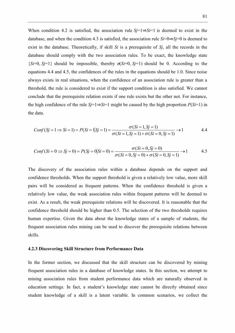
81

When condition 4.2 is satisfied, the association rule Sj=1⇒Si=1 is deemed to exist in the

database, and when the condition 4.3 is satisfied, the association rule Si=0⇒Sj=0 is deemed to

exist in the database. Theoretically, if skill Si is a prerequisite of Sj, all the records in the

database should comply with the two association rules. To be exact, the knowledge state

{Si=0, Sj=1} should be impossible, thereby σ(Si=0, Sj=1) should be 0. According to the

equations 4.4 and 4.5, the confidences of the rules in the equations should be 1.0. Since noise

always exists in real situations, when the confidence of an association rule is greater than a

threshold, the rule is considered to exist if the support condition is also satisfied. We cannot

conclude that the prerequisite relation exists if one rule exists but the other not. For instance,

the high confidence of the rule Sj=1⇒Si=1 might be caused by the high proportion P(Si=1) in

the data.

1)1,0()1,1(

)1,1()11()11(

SjSiSjSiSjSiSjSiPSiSjConf

4.4

1)1,0()0,0(

)0,0()00()00(

SjSiSjSiSjSiSiSjPSjSiConf

4.5

The discovery of the association rules within a database depends on the support and

confidence thresholds. When the support threshold is given a relatively low value, more skill

pairs will be considered as frequent patterns. When the confidence threshold is given a

relatively low value, the weak association rules within frequent patterns will be deemed to

exist. As a result, the weak prerequisite relations will be discovered. It is reasonable that the

confidence threshold should be higher than 0.5. The selection of the two thresholds requires

human expertise. Given the data about the knowledge states of a sample of students, the

frequent association rules mining can be used to discover the prerequisite relations between

skills.

4.2.3 Discovering Skill Structure from Performance Data

In the former section, we discussed that the skill structure can be discovered by mining

frequent association rules in a database of knowledge states. In this section, we attempt to

mining association rules from student performance data which are naturally observed in

education settings. In fact, a student’s knowledge state cannot be directly obtained since

student knowledge of a skill is a latent variable. In common scenarios, we collect the

82

performance data of students in assessments or tutoring systems and estimate their knowledge

states with the noisy observations. The evidence models that transfer the performance data of

students to their knowledge states have been investigated for several decades. The

psychometric models—the DINA and NIDA models (which have been discussed in chapter 3)

are used to infer the knowledge states of students from their response data on the multi-skill

test items. The well-known Bayesian Knowledge Tracing (BKT) model (Corbett and

Anderson 1995) (which have has been introduced in section 2.1.1.3) is used to update

students’ knowledge states according to the log files of their learning in a tutoring system. A

Q-matrix which represents the items to skills mapping is required in these models. The Q-

matrix is usually created by domain experts, but recently some researchers (Barnes 2005;

Desmarais and Naceur 2013; González-Brenes 2015) investigated to extract an optimal Q-

matrix from data. Our method assumes that an accurate Q-matrix is known, like the method in

(Scheines et al. 2014). Since the noise (e.g. slipping and guessing) is considered in the

evidence models, the probability that a skill is mastered by a student can be estimated. The

estimated knowledge state of a student is probabilistic, which incorporates the probability of

each skill mastered by the student. Table 4.1 shows an example of the database consisting of

probabilistic knowledge states. In the table, each record is a student’s knowledge state, and

attributes are skills. For example, the first record is the knowledge state of student “st1”,

incorporating the probabilities that skills S1, S2 and S3 are mastered by student, that is, 0.9,

0.8 and 0.9 respectively.

Table 4.1 A database of probabilistic knowledge states

Student ID Probabilistic Knowledge State

st1 {S1: 0.9, S2: 0.8, S3: 0.9}

st2 {S1: 0.2, S2: 0.1, S3: 0.8}

There are three types of uncertain data, that is, attribute uncertainty—each uncertain attribute

in a tuple is subject to its own independent probability distribution, correlated uncertainty—

multiple attributes are described by a joint probability distribution, and tuple uncertainty—all

the attributes of a tuple are subject to a joint probability distribution. Probabilistic knowledge

states are the data of attribute uncertainty, since each skill in a probabilistic knowledge state is

associated to a probability.

83

We discover prerequisite relations between skills from the probabilistic knowledge states of

students that are estimated by an evidence model. The frequent association rules mining can

no longer be used to discover the prerequisite relations between skills within a probabilistic

database, since a pattern in a probabilistic database is associated with a probability. A

probabilistic database can be interpreted as a set of deterministic instances (named possible

worlds) (Bernecker et al. 2009). We assume that the noise (e.g. slipping, guessing) causing

the uncertainty for different skills is mutually independent. In addition, we assume that the

knowledge states of different students are observed independently. Under these assumptions,

the probability of a possible world in our database is the product of the probabilities of the

attribute values over all the records in the possible world (Bernecker et al. 2009; Chui et al.

2007; Sun et al. 2010).

Table 4.2 Possible worlds of the probabilistic database in Table 4.1

ID Possible worlds Probability

1 st1: {S1=0, S2=0, S3=0} 0.001152

st2: {S1=0, S2=0, S3=0}

2 st1: {S1=1, S2=0, S3=0} 0.002592

st2: {S1=0, S2=0, S3=0}

3 st1: {S1=0, S2=0, S3=0} 0.000072

st2: {S1=1, S2=0, S3=0}

… … …

64 st1: {S1=1, S2=1, S3=1} 0.010368

st2: {S1=1, S2=1, S3=1}

Figure 4.1 The support count pmf of the pattern {S1=1, S2=1} in the database of Table 4.1

84

Table 4.2 shows the possible worlds of the probabilistic database in Table 4.1 as well as the

probability for each possible world. For example, the probability of the possible world that the

knowledge states of the students “st1” and “st2” are {S1=1, S2=1, S3=1} is about 0.0104 (i.e.

8.01.02.09.08.09.0 ). The support count of a pattern in a probabilistic database

should be computed with all the possible worlds. Thus the support count is no longer a

deterministic counted number but a discrete random variable. Figure 4.1 depicts the support

count probability mass function (pmf) of the pattern {S1=1, S2=1} in the database of Table

4.1. In the figure, for instance, the probability of σ (S1=1, S2=1) equal to 1 is about 0.7112,

which is the sum of the probabilities of all the possible worlds in which only one record

contains the pattern {S1=1, S2=1}. Since there are an exponential number of possible worlds

for a probabilistic database (e.g. 26 possible worlds for the database of Table 4.1), computing

the support count of a pattern is expensive. The Dynamic-Programming algorithm (Table 4.3)

proposed by Sun et al. (2010) is used to efficiently compute the support count pmf of a

pattern. The support count pmf Xf of pattern X is initialized to {1,0,…, 0} in step 2 (i.e. σ (X)

is zero before PDB is visited). Each ][kf X is updated when a tuple iT is visited (step 3 to 7),

where ))((][ kXSupPkf X , and Xip is the probability that pattern X occurs in tuple iT .

Table 4.3 Dynamic-Programming algorithm(Sun et al. 2010)

Input: probabilistic database PDB, pattern X

Output: support pmf XYf

1 begin

2 Initialize 0,,0,1 Xf

3 for each tuple iT in PDB do

4 010'X

XiX fpf

5 for 1k to n do

6 kfpkfpkf XXiX

XiX 11'

7 'XX ff

8 return Xf

9 end

85

To discover the prerequisite relations between skills from the probabilistic knowledge states

of students, the probabilistic association rules mining technique (Sun et al. 2010) is used,

which is an extension of the frequent association rules mining to discover association rules

from uncertain data. Since the support count of a pattern in a probabilistic database is a

random variable, the conditions 4.2 and 4.3 are satisfied with a probability. Hence the

association rules derived from a probabilistic database are also probabilistic. We use the

formula proposed by Sun et al. (2010) to compute the probability of an association rule

satisfying the two thresholds. It can be also interpreted as the probability of a rule existing in a

probabilistic database. For instance, the probability of the association rule Sj=1⇒Si=1 existing

in a probabilistic database is the probability that the condition 4.2 is satisfied in the database:

minconfnminconf

mmf SjSi

N

Nminsupnnf SjSi

minconfSiSjConfminsupSiSjSupPSiSjP1

01,01,1

111111

4.6

where N is the number of records in the database and 𝑓𝑋 denotes the support count pmf of

pattern X, and fX[k]=P(σ(X)=k).

The probability of the rule related to condition 4.3 is computed similarly. The algorithm (Sun

et al. 2010) implementing the computation of this formula is used. The algorithm is described

as Table 4.4.

According to formula 4.6, the probability of an association rule changes with the values of the

support and confidence thresholds. Given the two thresholds, the probability of an association

rule existing in a probabilistic database can be computed. And if the probability is very close

to 1.0, the association rule is considered to exist in the database. If both the association rules

related to a prerequisite relation are considered to exist, the prerequisite relation is considered

to exist. We can use another threshold, the minimum probability threshold denoted by

minprob, to select the most possible association rules. Thus, if both P(Sj=1⇒Si=1)≥minprob

and P(Si=0⇒Sj=0)≥minprob are satisfied, Si is deemed a prerequisite of Sj. When two skills

are estimated to be the prerequisite of each other, the relation between them is symmetric. It

means that the two skills are mastered or not mastered simultaneously. The skill models might

be improved by merging the two skills with the symmetric relation between them.

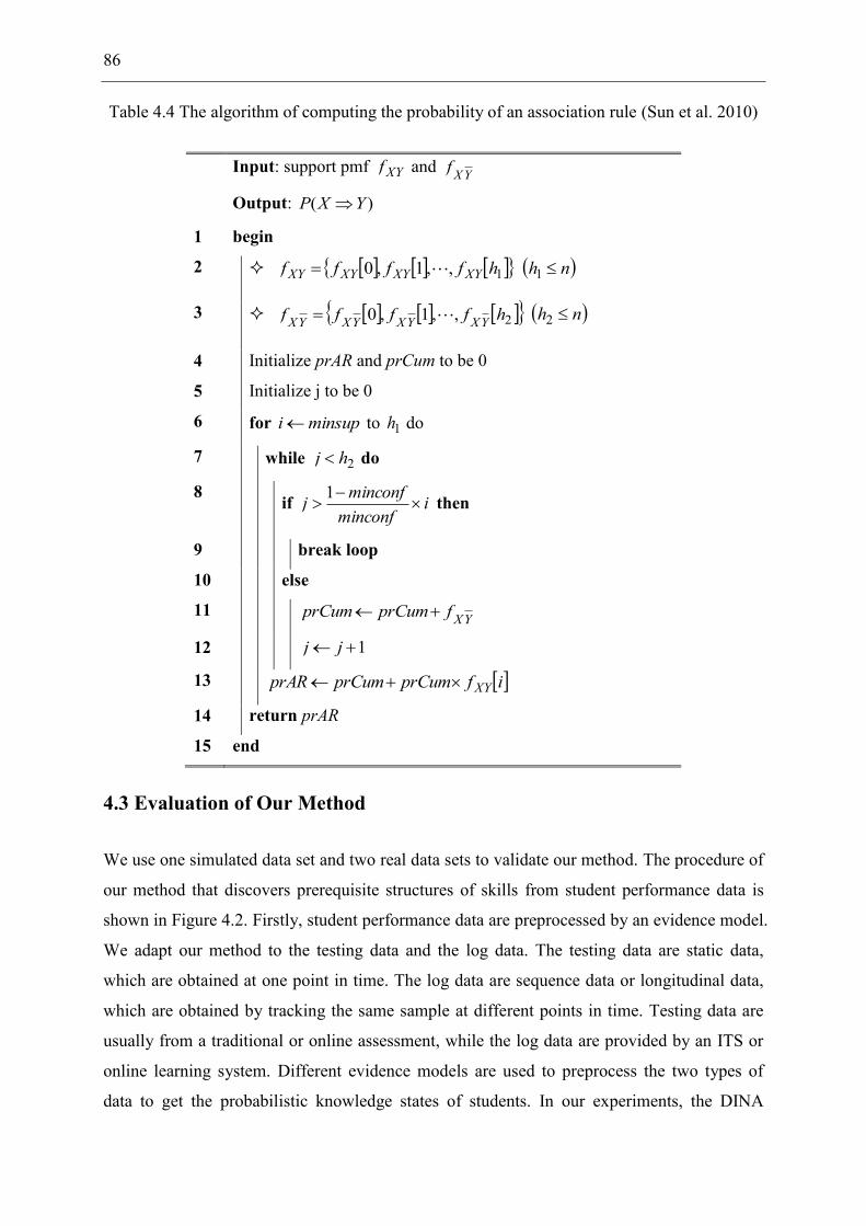
86

Table 4.4 The algorithm of computing the probability of an association rule (Sun et al. 2010)

Input: support pmf XYf and YXf

Output: )( YXP

1 begin

2 1,,1,0 hffff XYXYXYXY nh 1

3 2,,1,0 hffff YXYXYXYX nh 2

4 Initialize prAR and prCum to be 0

5 Initialize j to be 0

6 for minsupi to 1h do

7 while 2hj do

8 if i

minconfminconfj

1 then

9 break loop

10 else

11 YXfprCumprCum

12 1 jj

13 ifprCumprCumprAR XY

14 return prAR

15 end

4.3 Evaluation of Our Method

We use one simulated data set and two real data sets to validate our method. The procedure of

our method that discovers prerequisite structures of skills from student performance data is

shown in Figure 4.2. Firstly, student performance data are preprocessed by an evidence model.

We adapt our method to the testing data and the log data. The testing data are static data,

which are obtained at one point in time. The log data are sequence data or longitudinal data,

which are obtained by tracking the same sample at different points in time. Testing data are

usually from a traditional or online assessment, while the log data are provided by an ITS or

online learning system. Different evidence models are used to preprocess the two types of

data to get the probabilistic knowledge states of students. In our experiments, the DINA

87

model is used for the testing data, whereas the BKT model is used for the log data. Then the

probabilistic knowledge states of students estimated by the evidence model are used by the

probabilistic association rules mining to discover the strong association rules. Finally, the

prerequisite relations are determined in terms of the discovered association rules. To validate

our result, a straightforward method is to compare the results with the “true structure”. For the

simulated data, the discovered prerequisite structure is compared with the presupposed

structure that is used to generate the data. The presupposed structure is the “true structure”.

However, for the real data, the “true structure” is commonly difficult to be obtained. Thus in

our experiments, the prerequisite structure derived from the real data is compared with the

structure investigated by another research on the same dataset or the structure from human

expertise. We also evaluate whether the learned skill structures better explain student

performance data and whether they have the stronger predictive power than the flat models.

Figure 4.2 Procedure of discovering prerequisite structures of skills from performance data

4.3.1 The Experiment on Simulated Testing Data

Data set. We use the data simulation tool available via the R package CDM (Robitzsch et al.

2014) to generate the dichotomous response data according to a CDM (cognitive diagnostic

model, the DINA model used here). The prerequisite structure of the four skills is

presupposed as Figure 4.4 (a). According to this structure, the knowledge space decreases to

be composed of six knowledge states, that is ∅, {S1}, {S1, S2}, {S1, S3}, {S1, S2, S3}, {S1,

S2, S3, S4}. The reduced knowledge space implies the prerequisite structure of the skills. The

knowledge states of 1200 students are randomly generated from the reduced knowledge space

restricting every knowledge state type in the same proportion (i.e. 200 students per type). The

simulated knowledge states are used as the input of the data simulation tool. There are 10

simulated testing questions, each of which requires one or two of the skills for the correct

Evidence Model

Testingdata

Log data

DINA

BKT

...

ProbabilisticKnowledge

States

ProbabilisticAssociationRules Mining

Strong AssociationRules:S2=1=>S1=1S1=0=>S2=0...

S1

S2

Prerequisite Structure

88

response. The slip and guess parameters for each question are restricted to be randomly

selected in the range of 0.05 and 0.3. According to the DINA model with these specified

parameters, the data simulation tool generates the response data. The generated response data

approximately comply with the simulated knowledge states. Using the simulated response

data as the input of a flat DINA model, the slip and guess parameters of each question in the

model are estimated and the probability about each student’s knowledge of each skill is

computed. The tool for the parameter estimation of DINA model is also available through the

R package CDM (Robitzsch et al. 2014), which is performed by the Expectation

Maximization (EM) algorithm (Dempster et al. 1977) to maximize the marginal likelihood of

data.

The R package CDM is developed to provide functions to implement some famous cognitive

diagnosis models, such as DINA and NIDA, and some psychometric models, such as

multidimensional latent class IRT model, as well as some data sets. The functions used in this

experiment are “sim.din”, which is the data simulation tool, and “din”, which implements the

parameter estimation by EM algorithm for cognitive diagnosis models.

Result. The estimated probabilistic knowledge states of the simulated students are used as the

input data to discover the prerequisite relations between skills. For each skill pair, there are

two prerequisite relation candidates. For each prerequisite relation candidate, we examine

whether the two corresponding association rules Sj=1⇒Si=1 and Si=0⇒Sj=0 exist in the

database. The probability of an association rule existing in the database is computed

according to formula 4.6, which is jointly affected by the selected support and confidence

thresholds. For the sake of clarity, we look into the effect of one threshold leaving the other

one unchanged. The joint effect of the two thresholds will be discussed in section 4.3.4.

Giving a small constant to one threshold that all the association rules satisfy (perhaps several

trials are needed or simply assign 0.0), we can observe how the probabilities of the

association rules change with different values of the other threshold.

89

Figure 4.3 The probabilities of the association rules in the simulated data given different

confidence or support thresholds

Figure 4.3 (a) and (b) describe how the probabilities of the corresponding association rules in

the simulated data change with different confidence thresholds, where the support threshold is

given as a constant (0.125 here). When the probability of a rule is close to 1.0, the rule is

deemed to satisfy the thresholds. All the association rules satisfy the support threshold since

their probabilities are almost 1.0 at first. The rules in the two figures corresponding to the

same prerequisite relation candidate are depicted in the same color. In the figures, when the

confidence threshold varies from 0.2 to 1.0, the probabilities of the different rules decrease

from 1.0 to 0.0 in different intervals of threshold value. When we choose different threshold

90

values, different sets of rules will be discovered. In each figure, there are five rules that can

satisfy the significantly higher threshold. Given minconf=0.78, the probabilities of these rules

are almost 1.0 whereas others are almost 0.0. These rules are very likely to exist. Moreover,

the discovered rules in the two figures correspond to the same set of prerequisite relation

candidates. Accordingly, these prerequisite relations are very likely to exist. To make sure the

coverage of the association rules satisfying the high confidence threshold, it is necessary to

know the support distributions of these rules. Figure 4.3 (c) and (d) illustrate how the

probabilities of the corresponding association rules change with different support thresholds.

The confidence threshold is given as a constant 0.76, and five association rules in each figure

satisfy this threshold. Only on these rules, the effect of different support thresholds can be

observed. In each figure, the probabilities of the rules decrease in two intervals of threshold

value. For example, in Figure 4.3 (c), to select the rules corresponding to r3, r5 and r6, the

highest value for the support threshold is roughly 0.17, while for the other two rules, it is 0.49.

If both the confidence threshold and the support threshold are appropriately selected, the most

possible association rules will be distinguished from others. As a result, the five prerequisite

relations can be discovered in this experiment.

Figure 4.4 (a) Presupposed prerequisite structure of the skills in the simulated data; (b)

Probabilities of the association rules in the simulated data given minconf=0.76 and

minsup=0.125, brown squares denoting impossible rules; (c) Discovered prerequisite structure

Figure 4.4 (b) illustrates the probabilities of the corresponding association rules in the

simulated data given minconf=0.76 and minsup=0.125. A square’s color indicates the

probability of the corresponding rule. Five association rules in each of the figures whose

probabilities are almost 1.0 are deemed to exist. And the prerequisite relations corresponding

to the discovered rules are deemed to exist. To qualitatively construct the prerequisite

structure of skills, every discovered prerequisite relation is represented by an arc. It should be

S1

S2 S3

S4

(a) (b)

S1

S2 S3

S4

(c)(a)

91

noted that the arc representing the relation that S1 is a prerequisite of S4 is not present in

Figure 4.4 (a) due to the transitivity of prerequisite relation. Consequently, the prerequisite

structure discovered by our method which is shown in Figure 4.4 (c), is completely in

accordance with the presupposed structure shown in Figure 4.4 (a).

4.3.2 The Experiment on Real Testing Data

Data set. The ECPE (Examination for the Certification of Proficiency in English) data set is

available through the R package CDM (Robitzsch et al. 2014), which comes from a test

developed and scored by the English Language Institute of the University of Michigan

(Templin and Bradshaw 2014). This data set has also been used in section 3.4. A sample of

2933 examinees is tested by 28 items on 3 skills, i.e. Morphosyntactic rules (S1), Cohesive

rules (S2), and Lexical rules (S3). The parameter estimation tool in the R package CDM

(Robitzsch et al. 2014) for DINA model is also used in this experiment to estimate the slip

and guess parameters of items according to the student response data. And with the estimated

slip and guess parameters, the probabilistic knowledge states of students are assessed

according to the DINA model, which are the input data for discovering the prerequisite

structure of skills.

Result. The effect of different confidence thresholds on the association rules in the ECPE

data is depicted in Figure 4.5 (a) and (b) given the support threshold as a constant (0.25 here).

In each figure, there are three association rules that can satisfy a significantly higher

confidence threshold than others. The maximum value of the confidence threshold for them is

roughly 0.82. And these rules in the two figures correspond to the same set of prerequisite

relation candidates, that is, r4, r5 and r6. Thus these candidates are most likely to exist. It can

be noticed that in Figure 4.5 (a) the rule S3=1⇒S2=1 can satisfy a relatively high confidence

threshold. The maximum threshold value that it can satisfy is roughly 0.74. However, its

counterpart in Fig 4.5 (b), i.e. the rule S2=0⇒S3=0, cannot satisfy a confidence threshold

higher than 0.6. When a strong prerequisite relation is required, the relation corresponding to

the two rules cannot be selected. Only when both the two types of rules can satisfy a high

confidence, the corresponding prerequisite relation is considered strong. Likewise, the effect

of different support thresholds is shown in Figure 4.5 (c) and (d), where the confidence

threshold is given as 0.80. And in each figure, only the three association rules which satisfy

the confidence threshold are sensitive to different support thresholds. It can also be found that

these rules are supported by a considerable proportion of the sample. Even when minsup=0.27,

92

all the three rules in each figure satisfy it. According to the figures, when the support and

confidence thresholds are appropriately selected, these rules can be distinguished from others.

Consequently, the strong prerequisite relations can be discovered.

Figure 4.5 The probabilities of the association rules in the ECPE data given different

confidence or support thresholds

Given the confidence and support thresholds as 0.80 and 0.25 respectively, for instance, the

probabilities of the corresponding association rules are illustrated in Figure 4.6 (b). The rules

that satisfy the two thresholds (with a probability of almost 1.0) are deemed to exist, which

are evidently distinguished from the rules that do not (with a probability of almost 0.0). Three

prerequisite relations shown in Figure 4.6 (c) are found in terms of the discovered association

93

rules. To validate the result, we compare it with the findings of another research on the same

data set. The attribute hierarchy, namely the prerequisite structure of skills, in ECPE data has

been investigated by Templin and Bradshaw (Templin and Bradshaw 2014) as Figure 4.6 (a).

Our discovered prerequisite structure totally agrees with their findings.

Figure 4.6 (a) Prerequisite structure of the skills in the ECPE data discovered by Templin and

Bradshaw (2014); (b) Probabilities of the association rules in the ECPE data given

minconf=0.80 and minsup=0.25, brown squares denoting impossible rules; (c) Discovered

prerequisite structure

4.3.3 The Experiment on Real Log Data

Data set. We use the 2006-2007 school year data of the curriculum “Bridge to Algebra”

(Stamper et al. 2010) which incorporates the log files of 1146 students collected by Cognitive

Tutor, an ITS for mathematics learning. The units in this curriculum involve distinct

mathematical topics, while the sections in each unit involve distinct skills on the unit topic. A

set of word problems is provided for each section skill. This data set uses the general format

of data sets in Datashop (Koedinger et al. 2010), the well-known public repository of learning

interaction data developed by the Pittsburgh Science of Learning Center. Datashop provides

data on the interaction between students and educational software, including data from online

courses, ITSs, online assessment systems, collaborative learning environments, and

simulations. Table 4.5 shows several rows of the “Bridge to Algebra” data, where the column

attributes are selected for our experiment. The data provides the observations at the step level

and the problem level. In our experiment, we use the problem level observations, that is, when

all the “first attempts” in the scaffolding steps of a problem are correct, the problem is

S1

S2

S3

(a) (b)

S1

S2

S3

(c)( a )

94

recorded correct. Thus the values of attribute “Correct First Attempt” are grouped by values

of “Problem Name”. Each problem is an observation for a section skill.

Table 4.5 “Bridge to Algebra 2006-2007” data used in our experiment

Anon Student

Id

Problem Hierarchy Problem Name Step Name Correct First

Attempt

271823buwnj5 Unit EQUIVALENT-

FRACTIONS, Section

EQUIVALENT-FRACTIONS-1

EQFRAC1C001-6 MultiplyBy 1

271823buwnj5 Unit EQUIVALENT-

FRACTIONS, Section

EQUIVALENT-FRACTIONS-1

EQFRAC1C001-6 Fraction:UnitFractor 0

271823buwnj5 Unit EQUIVALENT-

FRACTIONS, Section

EQUIVALENT-FRACTIONS-1

EQFRAC1C001-6 GeneralHelpGoalNode 0

… … … …

271823buwnj5 Unit EQUIVALENT-

FRACTIONS, Section

EQUIVALENT-FRACTIONS-1

EQFRAC1S001-8 MultiplyBy 1

… … … …

Table 4.6 Skills in the curriculum “Bridge to Algebra”

Skill Problem Hierarchy Example

S1: Writing equivalent fractions Unit EQUIVALENT-FRACTIONS,

Section EQUIVALENT-FRACTIONS-

1&2

Fill in the blank:

632 .

S2: Simplifying fractions Unit EQUIVALENT-FRACTIONS,

Section EQUIVALENT-FRACTIONS-

3&4

Write the fraction in

simplest form:

3024 .

S3: Comparing and ordering fractions Unit EQUIVALENT-FRACTIONS,

Section EQUIVALENT-FRACTIONS-

5&6

Compare the

fractions 43 and

65 .

S4: Adding and subtracting fractions

with like denominators

Unit FRACTION-OPERATIONS-1,

Section FRACTION-OPERATIONS-

1&2

103

102

S5: Adding and subtracting fractions

with unlike denominators

Unit EQUIVALENT-FRACTIONS,

Section EQUIVALENT-FRACTIONS-

3&4

41

32

95

We use the sections in the units “equivalent fractions” and “fraction operations” as the skills.

The sections corresponding to the skills are shown in Table 4.6. There are 560 students in the

data set performing to learn one or several of the item-type skills in these units. The five skills

discussed in our experiment are instructed in the given order in Table 4.6. A student’s

knowledge of the prior skills has the potential to affect his learning of the new skill. Hence, it

makes sense to estimate whether a skill trained prior to the new skill is a prerequisite of it. If

the prior skill Si is a prerequisite of skill Sj, students who have mastered skill Sj quite likely

have previously mastered skill Si, and students not mastering the skill Si quite likely learn the

skill Sj with great difficulty. Thus if both the rules Sj=1⇒Si=1 and Si=0⇒Sj=0 exist in the

data, the prior skill Si is deemed a prerequisite of skill Sj.

Figure 4.7 Selected knowledge states inferred by BKT from log data

To discover the prerequisite relations between skills, firstly we need to estimate the outcomes

of student learning according to the log data. A student learns a skill by solving a set of

problems that requires applying that skill. At each opportunity, student knowledge of a skill

probably transitions from the unlearned to learned state. Thus their knowledge should be

updated each time they go through a problem. The BKT model has been widely used to track

the dynamic knowledge states of students according to their activities on ITSs. In the standard

BKT, four parameters are specified for each skill (Corbett and Anderson 1995): P(L0)

denoting the initial probability of knowing the skill a priori, P(T) denoting the probability of

student’s knowledge of the skill transitioning from the unlearned to the learned state, P(S) and

P(G) denoting the probabilities of slipping and guessing when applying the skill. We

implemented the BKT model by using the Bayes Net Toolbox for Student Modeling (Chang

et al. 2006), which facilitates training and evaluating DBNs. The parameter P(L0) is initialized

to 0.5 while the other three parameters are initialized to 0.1. The four parameters are

96

estimated according to the log data of students, and the probability of a skill to be mastered by

a student is estimated each time the student performs to solve a problem on that skill. In the

log data, students learned the section skills one by one and no student relearned a prior section

skill. If a prior skill Si is a prerequisite of skill Sj, the knowledge state of Si after the last

opportunity of learning it has an impact on learning Sj. We use the probabilities about

students’ final knowledge state of Si and Sj to analyze whether a prerequisite relation exists

between them (see Figure 4.7). Thus students’ final knowledge states on each skill are used as

the input data of our method.

Figure 4.8 The Probabilities of the association rules in the “Bridge to Algebra 2006-2007”

data given different confidence or support thresholds

97

Result. The probabilities of the association rules in the log data changing with different

confidence thresholds are illustrated in Figure 4.8 (a) and (b) given the support threshold as a

small constant (0.05 here). In Figure 4.8 (a), compared with the rules S4=1⇒S3=1 and

S5=1⇒S3=1, all the other association rules can satisfy a significantly higher confidence, while

in Figure 4.8 (b) if given minconf=0.6, only three rules satisfy it. The effect of different

support thresholds on the probabilities of the association rules is depicted in Figure 4.8 (c) and

(d) given the confidence threshold as a constant (0.3 here). All the association rules satisfy the

confidence threshold as the probabilities of the rules are almost 1.0 at first. In Figure 4.8 (c),

there are six rules that can satisfy a relatively higher support threshold (e.g. minsup=0.2). But

in Figure 4.8 (d), even given minsup=0.14, only the rule S4=0⇒S5=0 satisfy it, and the

maximum value for the support threshold that all the rules can satisfy is roughly 0.07.

Figure 4.9 (a) Prerequisite structure from human expertise; (b) Probabilities of the association

rules in the “Bridge to Algebra 2006-2007” data given minconf=0.6 and minsup=0.1, brown

squares denoting impossible rules; (c) Discovered prerequisite structure

Given the confidence and support thresholds as 0.6 and 0.1 respectively, the probabilities of

the association rules in the log data are depicted in Figure 4.9 (b). There are eight of the rules

in the form of Sj=1⇒Si=1 (left) and three of the rules in the form of Si=0⇒Sj=0 (right)

discovered, whose probabilities of satisfying the thresholds are almost 1.0. According to the

result, only the three prerequisite relations shown in Figure 4.9 (c), whose corresponding rules

both are discovered, are deemed to exist. Figure 4.9 (a) shows the prerequisite structure of the

five skills from the human experts’ opinions. It makes sense that the skills S1 and S2 rather

than skill S3 are required for learning the skills S4 and S5. This is supported by the chapter

warm-up content in the student textbook of the course (Hadley and Raith 2008). The

discovered rules in the form of Sj=1⇒Si=1 completely agree with the structure from human

S1

S2

S3 S4

S5

(a) (b) (c)

S1

S2

S3 S4

S5

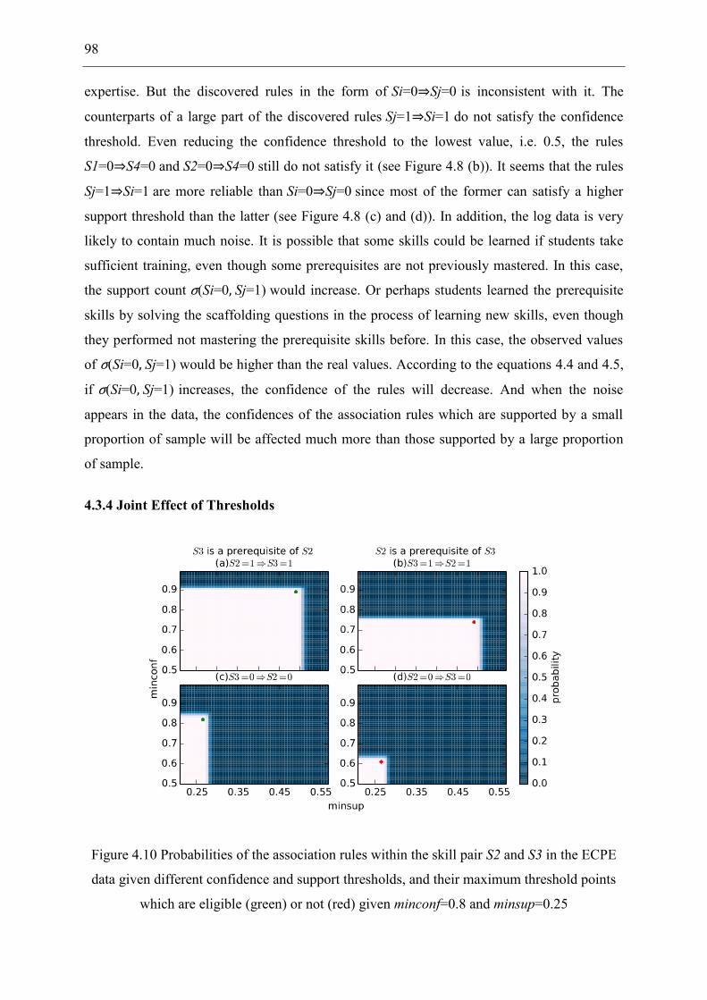
98

expertise. But the discovered rules in the form of Si=0⇒Sj=0 is inconsistent with it. The

counterparts of a large part of the discovered rules Sj=1⇒Si=1 do not satisfy the confidence

threshold. Even reducing the confidence threshold to the lowest value, i.e. 0.5, the rules

S1=0⇒S4=0 and S2=0⇒S4=0 still do not satisfy it (see Figure 4.8 (b)). It seems that the rules

Sj=1⇒Si=1 are more reliable than Si=0⇒Sj=0 since most of the former can satisfy a higher

support threshold than the latter (see Figure 4.8 (c) and (d)). In addition, the log data is very

likely to contain much noise. It is possible that some skills could be learned if students take

sufficient training, even though some prerequisites are not previously mastered. In this case,

the support count σ(Si=0, Sj=1) would increase. Or perhaps students learned the prerequisite

skills by solving the scaffolding questions in the process of learning new skills, even though

they performed not mastering the prerequisite skills before. In this case, the observed values

of σ(Si=0, Sj=1) would be higher than the real values. According to the equations 4.4 and 4.5,

if σ(Si=0, Sj=1) increases, the confidence of the rules will decrease. And when the noise

appears in the data, the confidences of the association rules which are supported by a small

proportion of sample will be affected much more than those supported by a large proportion

of sample.

4.3.4 Joint Effect of Thresholds

Figure 4.10 Probabilities of the association rules within the skill pair S2 and S3 in the ECPE

data given different confidence and support thresholds, and their maximum threshold points

which are eligible (green) or not (red) given minconf=0.8 and minsup=0.25

99

We have discussed the effect of one threshold on the probability of association rules while

eliminating the effect of the other one in the three experiments. To determine the values for

the thresholds, we investigate how the two thresholds simultaneously affect the probability of

an association rule. Figure 4.10 depicts how the probabilities of the association rules for the

skill pair S2 and S3 in the ECPE data change with different support and confidence thresholds,

where (a) and (c) involve one relation candidate while (b) and (d) involve the other one. The

figures demonstrate that the probability of a rule decreases almost from 1.0 to 0.0 when the

confidence and support thresholds vary from low to high. It can be found that the rules in the

left figures can satisfy an evidently higher confidence threshold than those in the right figures,

and have the same support distributions with them. If we set minconf=0.8 and minsup=0.25,

only the rules in the left figures satisfy them.

Figure 4.11 Maximum threshold points for the association rules in our three experiments,

where eligible points are indicated in green given the thresholds

Suppose that a rule satisfies the thresholds if its probability is higher than 0.95, i.e.

minprob=0.95. When we change the values of the confidence and support thresholds from 0.0

to 1.0, for each rule, we can find a point whose coordinates consist of the maximum values of

the confidence and support thresholds that the rule can satisfy. Finding the optimal point is

hard and there are probably several feasible points. To simplify the computation, the

thresholds are given by a sequence of discrete values from 0.0 to 1.0. We find the maximum

value for each threshold when only one threshold affects the probability of the rule given the

other as 0.0. And for each threshold, minprob is given as 0.97, roughly the square root of the

original value. The found maximum values for the two thresholds are the coordinates of the

point. The found point is actually an approximately optimal point. For convenience, the point

is named maximum threshold point in this thesis. The points for all the rules in the three data

100

sets are found by our method as well as plotted in Figure 4.11 (some points overlap). When

we set certain values to the thresholds, the points located in the upper right area satisfy them

and the related rules are deemed to exist. For one prerequisite relation, a couple of related

points should be verified. Only when both of them are located in the upper right area, they are

considered eligible to uncover the prerequisite relation. The eligible points in Figure 4.10 and

Figure 4.11 are indicated given the thresholds. In Figure 4.11 (c), some maximum threshold

points in the upper right area are not eligible as their counterpart points are not in the area.

4.4 Comparison with Existing Methods

In this chapter, we investigate whether the prerequisite structures discovered by the existing

methods from our data sets are consistent with our results. The likelihood method (Brunskill

2011) and the POKS algorithm (Desmarais et al. 2006) are examined using our data sets. Both

the two methods are adapted to our data in the experiments. Firstly, we will discuss how to

use the likelihood method to discover the prerequisite structure of skills from student

performance data. Then we will adapt the POKS algorithm to discover the prerequisite

structure of skills, which was proposed to discover prerequisite structures of observable

variables (i.e. items).

Application of the likelihood method

Brunskill (2011) proposed a method to determine prerequisite relations of skills by comparing

the maximum likelihood of the prerequisite model with that of the flat model (the skills are

independent). The model with the higher likelihood given the parameter values of the best fit

is preferred. That is, if the prerequisite model on a pair of skills has a higher maximum

likelihood, the prerequisite relation is deemed to exist. Conversely, if the flat model has a

higher maximum likelihood, the skills are considered independent. The author took into

account the uncertainty in measuring student knowledge from the noisy observations. In her

context, a question is related to only one skill. The BKT model is used as the evidence model.

And in her preliminary experiment, the noise parameters for observations are given by human

experts instead of learning from data. The parameters for skills are learned by the EM

algorithm to maximize the log-likelihood of data.

In our context, each question is related to multiple skills. For our testing data sets, we still use

the DINA model as the evidence model. We also use the pairwise evaluation. The likelihood

101

values of the prerequisite model and the flat model are computed under the formulism of

Bayesian networks in our experiments. Our experiment is implemented via the BNT package

(Murphy 2001). We construct the Bayesian network of the evidence model in terms of the Q-

matrix. For each pair of skills, the flat model is that no direct link is created between the

skills, while the prerequisite model is that a prerequisite link is created between the skills.

Two prerequisite models with different directions are tested for each pair of skills. And each

prerequisite model can be represented by two links in the Bayesian network. For example,

suppose skill Si is a prerequisite of skill Sj. When the direction of the link is from Si to Sj, the

parameters for the prerequisite link should be initialized as P(Sj=1 | Si=0)=0 and P(Sj=1 |

Si=1)=0.5. In the other case, when the direction of the link is from Sj to Si, the parameters for

the link should be initialized as P(Si=1 | Sj=0)=0.5 and P(Si=1 | Sj=1)=1. These parameters

specifications ensure the prerequisite relationship between the two skill nodes. For each

prerequisite model, we verified the two links with different directions. We use the EM

algorithm to learn the parameters that maximize the log-likelihood of the data. The parameters

P(Sj=1 | Si=1) and P(Si=1 | Sj=0) for the prerequisite links can be updated by the EM

algorithm, whereas the parameters P(Sj=1 | Si=0) and P(Si=1 | Sj=1) is deterministic and

cannot be changed. All the parameters for the observations are also updated by the EM

algorithm. As a result, the parameters of the best fit can be learned, and the maximum

likelihood of each model is computed.

Figure 4.12 Discovered prerequisite structures of skills using the likelihood method: (a)

simulated data; (b) the ECPE data

We select the model with the higher log-likelihood value between the prerequisite model and

the flat model for each skill pair. And when the prerequisite model in both directions has the

higher log-likelihood than the flat model, the prerequisite model is preferred. The resulting

102

prerequisite structures for the simulated data and the ECPE data (which are also used in

section 4.3) are illustrated in Figure 4.12. We can find that the prerequisite structure

discovered in the simulated data by the likelihood method is mostly consistent with the “true

structure” (see section 4.3). However, there are many disagreements between the structures

discovered in the ECPE data by the likelihood method and the finding of Templin and

Bradshaw (2014). Some erroneous links are found by the likelihood method. The result is

interpretable, since the likelihood method compares the prerequisite model with the flat model,

and the additional link in the prerequisite model is very likely to increase the model fit no

matter what the parameter values for the links. As a result, in the two data sets, our model

outperforms the likelihood method on the accuracy.

Application of the POKS algorithm

The POKS algorithm (Desmarais et al. 1996; Desmarais et al. 2006) learns the prerequisite

structure of the observable variables (items). To adapt the POKS algorithm to learn the

prerequisite structure of skills, firstly, we classify student knowledge states according to their

performance. The knowledge states classified here are deterministic. That is, we determine

whether each skill is mastered or non-mastered by a student. We still use the DINA model as

the evidence model and the probabilistic knowledge state of each student is estimated. When

the probability of a student mastering a skill is higher than 0.5, we suppose the student

mastered the skill; otherwise, the student have not mastered the skill. Thereby, the

deterministic knowledge state of each student can be determined. Then the POKS algorithm

can be used to learn the prerequisite structure of skills from the deterministic knowledge

states.

)()(

)(

)(

APBAPcpABP

cpBAP

4.7

The POKS algorithm determines whether a prerequisite relation exists in a pair of variables

(in the research of Desmarais and his colleagues, the variables represent items; in our

experiments, they represent skills). In their POKS algorithm, a prerequisite relation candidate

A→B is verified by three statistic tests on conditions 4.7, where Pc is the minimal conditional

probability for P(A|B) and )( BAP , which can be considered as an indicator of the

103

“strength” of prerequisite relations. The first two conditions ensure that the minimal “strength”

of the relation is above a predetermined threshold. The third condition is the conditional

independence test, which verifies that A and B interact with each other.

The first two conditions are verified by two binomial tests. The null hypotheses used in the

POKS algorithm for the two conditions are as equations 4.8. There is an important measure in

the hypothesis tests—p-value. The p-value is the probability of obtaining the observed sample

results, or “more extreme” results, when the null hypothesis is true. To calculate the p-value

of these null hypotheses, three frequency variables are needed, that is, BAN , , BAN , and

BAN , , which are the occurrences of the patterns in the database. The frequency variables

used in the POKS algorithm have the same meaning with the term “support count” in our

method. They stated that the frequency pairs ( BAN , , BAN , ) and ( BAN , , BAN , ) are the

stochastic variables and follow the binomial distribution, i.e. Bin(k, n, p), where for the pair

( BAN , , BAN , ), k is BAN , and p is )( BAP ; for the pair ( BAN , , BAN , ), k is BAN , and p

is )( ABP ; n equals to k+ BAN , . For an observed sample, given the null hypothesis

cpBAP , the “more extreme” results are the cases where k is greater than the BAN , of the

observed sample. Thus the p-value for the null hypothesis cpBAP can be calculated as

the probability in the binomial distribution when k equal and greater than BAN , , which is

depicted as equation 4.9. Please note that the p-value computed here is expressed differently

from that in the paper of Desmarais et al. (1996), but the result should be the same. The p-

value of the other null hypothesis is computed in the same way.

H0: cpBAP , cpABP )( 4.8

p-value= knc

kc

n

NkBA pp

kn

NkpnbinBA

)1(),,(

,

, 4.9

The significance level (also called the error tolerance level) denoted by αc is predetermined.

When the p-value computed in equation 4.9 is smaller than the significance level, the null

hypothesis will be rejected. As a result, the alternative hypothesis cpBAP will be

accepted. If the p-value is greater than the significance level, it is failed to reject the

hypothesis.

104

The third condition in conditions 4.7 is verified by the χ2 (Chi-square) test. Chi-square test is a

statistical test commonly used to compare observed data with the data we expect to obtain

given a specific hypothesis. The null hypothesis for the third condition in conditions 4.7 is as

equation 4.10, that is, A and B are independent with each other. There are three steps to

compute the p-value of the observed sample given the null hypothesis. The first step is to

calculate the degrees of freedom DF=(LA-1)*(LB-1), where LA and LB are the number of

alternatives of variable A and B. In our test, A and B are the binary variable, thus the DF=1.

In the second step, we calculate the chi-square value given the null hypothesis. According to

the null hypothesis, the expected co-occurrence of A and B should be (𝑁𝐴 ∗ 𝑁𝐵) 𝑁⁄ , where N

is the sample size. Thus the chi-square value of the observed sample is computed as equation

4.11. In the final step, the p-value is computed with the degrees of freedom and the chi-square

value in terms of Chi-Square Distribution. Likewise, when the p-value is smaller than the

significance level αi, the null hypothesis is rejected. Thereby, A and B are not independent. If

the p-value is greater than the significance level αi, the null hypothesis is accepted. In this

case, A and B are independent with each other.

)()( APBAP 4.10

NNNN

NNN BA

BABA ** 2

,2

4.11

We apply the three statistic tests for the estimated deterministic knowledge states to discover

the prerequisite structure of skills. In our experiments, the pc is given 0.8 or 0.9, while both

the significance levels αc and αi are given 0.1. The p-values of the three tests for each skill

pair are computed. Comparing the p-values with the significance levels, when all the p-values

are below the significance levels, the prerequisite relation exists in the skill pair; otherwise,

the skill pair has no prerequisite relation. The discovered prerequisite structures of skills in

the simulated data and the ECPE data given different values of “strength” indicator pc are

depicted in Figure 4.13. In this figure, it can be found that the value of the “strength” indicator

pc affects the discovered structures. The parameter pc is similar to the confidence threshold in

our method. In the experiments, the POKS algorithm is used to discover prerequisite structure

of skills from the deterministic knowledge states. This two-phase application of the POKS

algorithm also relies on the accuracy of the evidence model. Moreover, the deterministic

knowledge states used by the POKS algorithm are the most possible classes of student

105

knowledge state, which eliminate the other possibilities. The probabilistic knowledge states

used by our method indicate all the possibilities of the student knowledge states. They are

more informative than the deterministic knowledge states, which should lead to more accurate

analysis on skill structure.

Figure 4.13 Discovered prerequisite structures of skills using the POKS algorithm: (a) the

simulated data; (b) the ECPE data

4.5 Improvement of a Student Model via Prerequisite Structures

In this section, we evaluate whether the prerequisite structures of skills discovered by our

method improve the performance of student models. We compare the model incorporating the

prerequisite structure of skills with the original model on the fit to data and the prediction

accuracy. The simulated testing data and the real testing data (used in section 4.3) are used for

the evaluation. The evidence model for the two data sets is the DINA model. For each data

set, two experiments are implemented. In the first experiment, there is no link between the

skills. In the second experiment, the discovered prerequisite structure of the skills is used.

The experiments are implemented via the BNT package (Murphy 2001). A Bayesian network

for each experiment is created. The parameters of the Bayesian network are learned by the

EM algorithm. In the second experiment, the prerequisite relations between skills are

represented by the links between the skill nodes, and the directions are from the prerequisites

to the other skills. That is, if Si is a prerequisite of Sj, the link between the two skills in the

Bayesian network is 𝑆𝑖 → 𝑆𝑗. And the parameters is initialized as P(Sj=1 | Si=0)=0 and P(Sj=1

| Si=1)=0.5. Thus the prerequisite relations are regarded as deterministic relations in the

106

experiments. If a skill has multiple prerequisites, like the skill S4 in the simulated data (see

section 4.3) which has three prerequisites, i.e. S1, S2 and S3, the parameters is initialized as

P(Sj=1 | if any prerequisite is 0)=0 and P(Sj=1 | all the prerequisites are 1)=0.5. Please note

that the transitivity cannot be expressed by the prerequisite links in the Bayesian network.

Thus all the discovered prerequisite relations should be represented by the links in the

Bayesian network. For example, in the simulated data, there should be a link from S1 to S4.

And in the ECPE data, there should be a link from S3 to S1. Using our specification, the noise

parameter P(Sj=1 | Si=1) can be learned from data by the EM algorithm. We also can give a

“soft” specification for the parameter P(Sj=1 | Si=0), like 0.1. Then this parameter can be also

learned from data. In this experiment, we assume the prerequisite relationship between skills

is deterministic.

Table 4.7 The log-likelihood values of the model with the prerequisite structure and the

original model

Original model Model with the prerequisite structure

Simulated data -6734 -6514

ECPE data -43259 -41944

As introduced in section 2.1.1.1, the EM algorithm learns the parameter values which

maximize the likelihood of data. The maximum log-likelihood of each model is computed.

Table 4.7 shows the log-likelihood values of the model with the prerequisite structure

estimated by our method in section 4.3 and the original model. The models are tested by using

the simulated data and the ECPE data. We can find that the model with the prerequisite

structure of skills has a significant higher log-likelihood value than the original model

(without links between skills) on both of the data sets. Therefore, the prerequisite structure

estimated by our method improves the model fit to data.

Besides the model fit to data, we also investigate whether the prerequisite structure improves

the accuracy of a student model on predicting student knowledge states and their

performance. We use the 4-fold cross-validation to estimate the accuracy of the two models

(with and without the prerequisite structure). In the simulated data, the knowledge state of

each student is known, which is generated simultaneously with the response data. Thereby we

estimate the accuracy of the two models for knowledge estimation. After the parameters in the

Bayesian network of each model are learned by the EM algorithm using the training data,

107

giving the response record of a student in the test data as the evidence, the probability that the

student mastered each skill can be inferred by the Bayesian network. When the probability of

mastering a skill is higher than 0.5, we suppose that the student mastered that skill; otherwise,

the student has not mastered that skill. The estimated knowledge state of each student is

compared with the “true” knowledge state. And the accuracy is the percentage of the correct

predictions of student knowledge states in the data set.

In the ECPE data, the “true” knowledge states of students are unknown. Thus we estimate the

accuracy of predicting student performance on unseen items. For each pair of training and

testing data, the process is similar to the performance prediction used in chapter 3. For each

student in the test data, the response to one of the items is hidden, and the responses to the

remaining items are used as the evidence. Then, the probability of the student giving the

correct answer to the unseen item is predicted by the Bayesian network. When the probability

is higher than 0.5, we suppose that the student will give a correct answer to the unseen item;

otherwise, the student will response incorrectly. We iteratively hide each item in the test data,

and use the observations on the remaining items to predict student performance on the unseen

item. And we compare the predictions with the “real” observations, and the prediction

accuracy is computed as the percentage of the correct predictions in the total number of

predictions. The accuracy values of the two models on the performance prediction are shown

in Table 4.8. We also calculate the RSME values of the two models, which are also shown in

Table 4.8. We see that the model with the prerequisite structure have the better accuracy and

RSME values than the original model on both of the data sets. Therefore, prerequisite

structures can improve the prediction accuracy of a student model.

Table 4.8 The model with the prerequisite structure vs. the original model

Original model Model with the prerequisite structure

Simulated

data

Accuracy 0.7780 0.7913

RSME 0.4712 0.4568

ECPE

data

Accuracy 0.7443 0.7451

RSME 0.5057 0.5049

We estimate the knowledge estimation accuracy of the two models on the simulated data with

different numbers of observations (i.e. items). The resulting accuracy values of the two

models given different numbers of observations are depicted in Figure 4.14. We can find that

108

the accuracy of the model with the prerequisite structure is significantly higher than that of

the original model. Therefore, the prerequisite structure improves the accuracy of the student

model. This finding also makes sense in principle. That is, when a student’s response to an

item is observed, student knowledge of the skills related to the item will be updated. The

observation also gives some implicit information about student knowledge of the prerequisite

skills, although no direct observation is given on them. For example, if a student gives a

correct answer to an item, the probabilities that the student mastered the related skills should

be increased. The belief of the student mastering the prerequisite skills should also be

increased. The model with the prerequisite structure of skills can propagate the information of

observations to the skills not directly related through the prerequisite links.

Figure 4.14 The student model with the prerequisite structure vs. the original student model

4.6 Summary

The prerequisite structures of fine-grained skills are the basis for determining the individual

learning sequence. Constructing the prerequisite structures requires much knowledge

engineering effort. Discovering prerequisite structures of skills from student performance data

is challenging, since student knowledge of skills are latent variables. In this chapter, firstly we

review the existing methods of extracting prerequisite structures from data. The existing

methods to learn skill structures from data have not been reliably and empirically evaluated.

Then we propose a novel method to learn prerequisite structures of skills from student

performance data. Since a prerequisite link corresponds to two association rules, we learn the

skill structures by discovering association rules from data. However, we cannot directly

observed student knowledge of skills. Thus we use a two-phase method. In the first phase,

student performance data is preprocessed by an evidence model. In the second phase, the

109

probabilistic knowledge states of students estimated by the evidence model are used as the

input data of probabilistic association rules mining. Prerequisite links between skills are

determined by discovering association rules from student probabilistic knowledge states. We

use one simulated data set and two real data sets to evaluate our method. We adapt our

method to two common types of data, the testing data and the log data, which are

preprocessed by different evidence models, the DINA model and the BKT model. The

structures discovered by our method are compared with presupposed structure in the

simulated data, or the structure found by another research or that from expertise. The results

show that our method “correctly” discovered the structures in the testing data and partially

discovered the structure in the log data. Applying our method in the log data needs to be

improved. Determining the appropriate confidence and support thresholds is a crucial issue in

our method. The maximum threshold points of the probabilistic association rules are used for

determining the thresholds. However, selecting the association rules is still a problem, which

can be further studied. The prerequisite structures of skills discovered by our method can be

applied to assist human experts on skill modeling or to validate the prerequisite structures of

skills from human expertise. We also compare our method with other existing methods. We

apply the likelihood method proposed by Brunskill (2011) and the POKS algorithm proposed

by Desmarais et al. (2006) to learn skill structures from the testing data. The POKS algorithm

performs well on extracting skill structures from data, whereas the likelihood method does

not. Determining the “strength” parameter (i.e. pc) in the POKS algorithm is also a problem as

giving the values to the thresholds in our method. Finally, we verify that the prediction

accuracy of a student model can be improved by incorporating the prerequisite structure of

skills.

110

111

Chapter 5: Conclusion

We have presented our work towards improving different layers of a student model for

individualized learning. Individualized learning is recognized more effective than the

conventional learning (Desmarais and Baker 2012). It is the main goal of computer-based

learning systems. Student models are the foundation for individualized learning. Improving

student models is an active issue for the ITS and AIED communities. A good student model

should precisely distinguish student knowledge by recognizing student behaviors. The more

precisely a student model distinguish students, the better the individualized feedback can be

designed. In addition, a good student model should be able to interpret the latent

characteristics of student learning, like the learning sequence. Our work presented in chapters

3 and 4 improves a student model in the two aspects. In this chapter, we summarize our work

from several perspectives. Moreover, we discuss the limitations of our work in this thesis and

some ideas for the future research.

5.1 Summary of This Thesis

Individualized learning improves the learning achievement by providing learning contents

which are adaptive to student current knowledge. A student model is the basis for

individualized learning. The accuracy of a student model affects the individualized learning.

A student model is used to distinguish student knowledge by recognizing student behaviors.

Since noise exists in student behaviors, a student model should be capable to handle the

uncertainty when transferring student behaviors to knowledge. A student model can contain

multiple layers. We divide a student model into two parts according to different issues are

treated in these layers—the evidence model and the skill model. The evidence model is used

to handle the uncertainty in transferring student behaviors to knowledge. The skill model is

used to represent the latent variables that measure student knowledge and the relationships

among them. We have reviewed the prevalent evidence models, each of which is in a

formulism to handle the uncertainty. We have also reviewed the common relationships in a

skill model and the probabilistic methods to represent these relationships.

Based on the knowledge of existing student models, we focus on two aspects to improve a

student model for individualized learning. One is the diagnostic ability of a student model.

Most of current student models are binary. Student behaviors are measured by success/failure

112

variables. We introduce the diagnostic items to more precisely distinguish student behaviors.

Some erroneous behaviors are labeled by the corresponding knowledge biases, and then

recognized and transferred by our diagnostic model. The other one is the expressive ability of

a student model. Learning sequence is an importance characteristic of human knowledge

acquisition. The cognitive order is expressed by the prerequisite relationships among

knowledge components. Incorporating the prerequisite structure of knowledge components

enables a student model to capture the cognitive order. A student model complying with the

learning characteristics and laws can better interpret and predict student behaviors. However,

acquiring prerequisite structures of skills is a tough and time-consuming task. Student

knowledge on a skill is a latent variable. Extracting prerequisite structures of skills from

student performance data is challenging. We propose a two-phase method to learning skill

structures from data. In the first phase, student performance data are transferred to

probabilistic knowledge states by an evidence model. In the second phase, we learn the

prerequisite structure of skills from the probabilistic knowledge states. Probabilistic

association rules mining is an emerging data mining technique for discovering association

rules from uncertain data. We apply this technique to discovering the skills pairs with the

prerequisite relationship.

We evaluate our diagnostic model with simulated data and real data. The simulated data is

generated based on the parameter values from real data. This strategy makes the simulated

data close to the real data. We evaluate the accuracy of our diagnostic model in knowledge

estimation and performance prediction. The accuracy of knowledge estimation is only

evaluated for simulated data, since in real scenarios a student’s real knowledge is unknown.

We use k-fold cross-validation to estimate the model accuracy. The knowledge estimation

accuracy is calculated by comparing the predictions of unseen students’ knowledge states

with their real states. The performance prediction accuracy is calculated by comparing the

predictions of unseen responses with the observed responses. We compare our diagnostic

models with other two diagnostic models. Since the differences between the three models are

the model complexity (the number of parameters) and the assumptions of the noise assigned

for observations, we firstly compare the three models on the model fit and complexity. In two

data sets, the MC-DINA model has the best AIC and BIC values. Then we compare the

accuracy of the three models. Our model has a competing performance on student

performance prediction. Furthermore, we compare our model and other two diagnostic

models with three binary models. The three binary models have the same structures with the

113

diagnostic models. And the results demonstrate that the diagnostic models significantly

outperform the binary models on knowledge estimation, and slightly better than binary

models on performance prediction.

We evaluate our two-phase method of learning skill structure from data using one simulated

data set and two real data sets. Among the two data sets, one is the testing data, and the other

is the log data. The simulated data is the testing data. To generate the simulated data, we

presuppose a prerequisite structure of skills. And the simulated knowledge states are restricted

to comply with the prerequisite structure. For the testing data, we use the DINA model to

estimate student probabilistic knowledge states. For the log data, we use the BKT model to

estimate student knowledge states. And the final knowledge states of each skill are used to

extract the prerequisite structure. The prerequisite structure discovered in the simulated data is

compared with the presupposed structure, while the structure discovered in the real testing

data is compared with the finding of another research (Templin and Bradshaw 2014) on the

same dataset. And the structure derived from the log data are compared with the structure

from human expertise. The results demonstrate that our method performs well to discover the

prerequisite structure of skills from the testing data, but not well for the log data. The log data

might contain much noise from student learning. Applying our method to the log data needs

to be improved. At last, we also verify whether the accuracy of a student model is improved

by introducing the prerequisite structure of skills. We compare the model incorporating the

prerequisite structure with the original model. The results demonstrate that the accuracy of the

model is significantly improved by introducing the prerequisite structure.

In the theoretical perspective, on one hand, we extend a popular student model—the NIDA

model for polytomous data. The polytomous data are the student responses to multiple choice

questions. On the other hand, we propose a two-phase method to learn the structure of latent

variables from noisy data. The structure of latent variables is the prerequisite structure of

skills. In the application perspective, our diagnostic model for responses to multiple choice

questions can be easily extended to model general erroneous response data. The requirement

is only that student systematic errors are collected and labels with knowledge biases. Our

method to learn prerequisite structures of skills can be used to assist human experts in skill

modeling or to validate the prerequisite structures of skills from human expertise.

114

5.2 Limitations and Future Research

Our work towards improving student models for individualized learning has been presented.

In this section, we discuss the limitations of our work and some possible directions for the

future research. Our work can be improved in some aspects and the direction of improving

student modeling for individualized learning can be further studied.

Our diagnostic model in this thesis is specified to deal with student responses to multiple

choice items. If student erroneous responses can be collected and labeled with corresponding

knowledge biases, our model can be easily generalized to deal with student erroneous

responses to any type of items, like open-ended items. Moreover, student knowledge on a

skill is measured by a binary variable with the values 1 (mastered) and 0 (not mastered). The

knowledge biases used in our model actually indicate lack of knowledge on some skills. The

misconceptions are not incorporated in our model. If erroneous responses are associated with

misconceptions, our diagnostic model can be extended to incorporate misconceptions by

measuring student knowledge with a multinomial variable. Recognizing student systematic

errors in open-end items requires a lot of knowledge engineering effort. Associating errors

with misconceptions is also a tough and time-consuming task. The existing methods of

automatically generating errors (VanLehn 1990; Paquette et al. 2012; Guzmán et al. 2010)

need to be empirically studied. The automatically generated errors might be verified with a

diagnostic student model. Student erroneous behaviors provide much diagnostic information,

which can enhance the individualized learning. Further researches to improve the diagnostic

ability of a student model are necessary.

Nowadays, a large number of ITSs and online learning environments provide plenty of

learning data for researchers to analyze, in order to improve student learning achievement

with deeper individualization. In recent two decades, many researchers have been investigated

to analyze sequence data from ITSs by using educational data mining techniques. The state of

the art technique for modeling the sequence data is the BKT model. There are plenty of

variants for the BKT model (see section 2.1.1.3). However, most of the variants still focus on

binary performance data. Our diagnostic model is an extension of a static student model (i.e.

NIDA). It can be extend for sequence data by using a dynamic Bayesian network. The BKT

model is a special dynamic Bayesian network model, which accounts for the transitioning of

student knowledge state during learning. And in the original BKT model, an observation is

115

only related to one skill. The multiple subskills are considered in a variant of the BKT model

(Xu and Mostow 2011). And a recent general framework (González-Brenes et al. 2014) is

proposed to integrate arbitrary features into the BKT model. Based on these researches, the

diagnostic feature—student erroneous responses perhaps can be introduced into the BKT

model.

Some other diagnostic features have been introduced into the BKT model. A recent research

extended the BKT model to allow partial credit data (Wang and Heffernan 2013). They took

into account the attempt and hint data from an ITS, and designed an reward and penalty

mechanism to score student performance. The observations in their BKT model are measured

by a continuous variable. However, their work assumed that the continuous performance

variables and the slip and guess parameters follow the Gaussian distribution. The parameters

of the Gaussian distributions are learned for the fit of the model. Although it is shown that

their model outperforms the traditional BKT model, their model is not optimized. Dealing

with the partial credit data is necessary in some educational environments. For example,

student behaviors in a game-based learning environment cannot be measured by a binary

variable. Student actions in educational games are usually scored by a reward and penalty

mechanism. Thus the performance data are usually the ordered continuous values. Student

models for partial credit data need to be further investigated.

Item difficulty is also an important feature in student learning. In probabilistic graphical

models, like the BKT model and the NIDA model, the items are not distinguished. Our

preliminary work presented in section 3.4 has empirically discussed the relationship between

item difficulty and the probability of slipping/guessing on an item. Recently, the LFKT model

(Khajah et al. 2014a) integrates the IRT model and the BKT model. The item difficulty and

student ability are introduced into the BKT model for individualizing the slip and guess

parameters.

Our method to discover prerequisite structures of skills from data performs well on testing

data, but not on the log data. The final knowledge state of a student on each skill in the log

data is used for discovering prerequisite relations. However, the final knowledge states of

students might not comply with the prerequisite relations of skills. The log data (or

longitudinal data) are more complex than the testing data. Student knowledge is time-

sensitive. As discussed in section 4.3.3, a student’s knowledge state on some skills might be

implicitly changed during learning other skills, which results in the real knowledge state

116

inconsistent with the historical data. A further study on applying our method in log data is

needed. Another limitation is that our method relies on an accurate Q-matrix. The Q-matrix is

usually studied by human experts. However, when the Q-matrix contains some biases, the

accuracy of our model will be affected. The effect of the Q-matrix on our method need to be

further studied. Or a method directly learning the skill structure from performance data

without requiring a Q-matrix can be investigated in future work.

Student modeling has been developed for ITSs for several decades. There are many

competing student models, which provide the accurate estimation of student knowledge. In

recent years, the emerging learning environments—MOOCs attract the interest of a lot of

educators and researchers. Tracking student knowledge and analyzing learning characteristics

in MOOCs is an active issue. Modeling large scale sequence data become a challenging

problem. And individualized learning for the new kind of educational environments can be a

good direction for future research.

117

Bibliography

Agrawal, R., Imieliński, T., and Swami, A. (1993). Mining association rules between sets of items in large databases. In, Proceedings of the 1993 ACM SIGMOD international conference on Management of data. ACM, Washington, D.C., USA, pp. 207-216.

Agrawal, R., and Srikant, R. (1994). Fast Algorithms for Mining Association Rules in Large Databases. In, Proceedings of the 20th International Conference on Very Large Data Bases. Morgan Kaufmann Publishers Inc., pp. 487-499.

Aleven, V., McLaren, B. M., and Sewall, J. (2009). Scaling up programming by demonstration for intelligent tutoring systems development: An open-access web site for middle school mathematics learning. IEEE Transactions on Learning Technologies 2 (2):64-78.

Baker, F. B. (2001). The basics of item response theory. ERIC.

Baker, R. J. d., Corbett, A., and Aleven, V. (2008). More Accurate Student Modeling through Contextual Estimation of Slip and Guess Probabilities in Bayesian Knowledge Tracing. In Woolf, B., Aïmeur, E., Nkambou, R., and Lajoie, S. (eds), Proceedings of the 9th International Conference on Intelligent Tutoring Systems. Springer Berlin Heidelberg, pp. 406 - 415.

Baker, R. J. d., Corbett, A., Gowda, S., Wagner, A., MacLaren, B., Kauffman, L., Mitchell, A., and Giguere, S. (2010a). Contextual Slip and Prediction of Student Performance after Use of an Intelligent Tutor. In De Bra, P., Kobsa, A., and Chin, D. (eds), User Modeling, Adaptation, and Personalization. Springer Berlin Heidelberg, pp. 52-63.

Baker, R. J. d., Goldstein, A., and Heffernan, N. (2010b). Detecting the Moment of Learning. In Aleven, V., Kay, J., and Mostow, J. (eds), Proceedings of the 10th International Conference on Intelligent Tutoring Systems. Springer Berlin Heidelberg, pp. 25-34.

Baker, R. S. J. D., Pardos, Z. A., Gowda, S. M., Nooraei, B. B., and Heffernan, N. T. (2011). Ensembling predictions of student knowledge within intelligent tutoring systems. In, Proceedings of the 19th international conference on User modeling, adaption, and personalization. Springer-Verlag, Girona, Spain, pp. 13-24.

Barnes, T. (2005). The Q-matrix method: Mining student response data for knowledge. In, American Association for Artificial Intelligence 2005 Educational Data Mining Workshop.

Barnes, T., Bitzer, D., and Vouk, M. (2005). Experimental analysis of the q-matrix method in knowledge discovery. In, Foundations of intelligent systems. Springer. pp. 603-611.

Beck, J., Chang, K.-m., Mostow, J., and Corbett, A. (2008). Does Help Help? Introducing the Bayesian Evaluation and Assessment Methodology. In Woolf, B., Aïmeur, E., Nkambou, R., and Lajoie, S. (eds), Proceedings of the 9th International Conference on Intelligent Tutoring Systems. Springer Berlin Heidelberg, pp. 383-394.

118

Beck, J. E., and Chang, K.-m. (2007). Identifiability: A fundamental problem of student modeling. In, User Modeling 2007. Springer. pp. 137-146.

Beck, J. E., and Sison, J. (2004). Using knowledge tracing to measure student reading proficiencies. In, Proceedings of the 7th International Conference on Intelligent Tutoring Systems. Springer, pp. 624-634.

Beheshti, B., and Desmarais, M. (2012). Improving matrix factorization techniques of student test data with partial order constraints. In, User Modeling, Adaptation, and Personalization. Springer. pp. 346-350.

Beheshti, B., and Desmarais, M. C. (2015). Goodness of fit of skills assessment approaches: Insights from patterns of real vs. synthetic data sets. In, Educational Data Mining.

Beheshti, B., Desmarais, M. C., and Naceur, R. (2012). Methods to Find the Number of Latent Skills. In, Educational Data Mining. pp. 81-86.

Bernecker, T., Kriegel, H.-P., Renz, M., Verhein, F., and Zuefle, A. (2009). Probabilistic frequent itemset mining in uncertain databases. In, Proceedings of the 15th ACM SIGKDD international conference on Knowledge discovery and data mining. ACM, Paris, France, pp. 119-128.

Borman, S. (2009). The Expectation Maximization Algorithm A short tutorial.

Brandherm, B., and Jameson, A. (2004). An extension of the differential approach for Bayesian network inference to dynamic Bayesian networks. International Journal of Intelligent Systems 19 (8):727-748.

Brown, J. S., and VanLehn, K. (1980). Repair theory: A generative theory of bugs in procedural skills. Cognitive science 4 (4):379-426.

Brunskill, E. (2011). Estimating Prerequisite Structure From Noisy Data. In, Educational Data Mining. pp. 217-222.

Brusilovsky, P., and Peylo, C. (2003). Adaptive and intelligent web-based educational systems. International Journal of Artificial Intelligence in Education 13:159-172.

Carmona, C., and Conejo, R. (2004). A Learner Model in a Distributed Environment. In De Bra, P. E., and Nejdl, W. (eds), Proceedings of the 3rd International Conference on Adaptive Hypermedia and Adaptive Web-Based Systems. Springer Berlin Heidelberg, pp. 353-359.

Carmona, C., Millán, E., Pérez-de-la-Cruz, J. L., Trella, M., and Conejo, R. (2005). Introducing Prerequisite Relations in a Multi-layered Bayesian Student Model. In Ardissono, L., Brna, P., and Mitrovic, A. (eds), Proceedings of the 10th International Conference on User Modeling Springer Berlin Heidelberg, pp. 347-356.

Cen, H., Koedinger, K., and Junker, B. (2006). Learning Factors Analysis – A General Method for Cognitive Model Evaluation and Improvement. In Ikeda, M., Ashley, K., and Chan, T.-W. (eds), Proceedings of the 8th International Conference on Intelligent Tutoring Systems. Springer Berlin Heidelberg. pp. 164-175.

119

Chang, K.-m., Beck, J., Mostow, J., and Corbett, A. (2006). A bayes net toolkit for student modeling in intelligent tutoring systems. In, Proceedings of the 8th international conference on Intelligent Tutoring Systems. Springer-Verlag, Jhongli, Taiwan, pp. 104-113.

Chen, Y., Wuillemin, P.-H., and Labat, J.-M. (2014). Bayesian Student Modeling Improved by Diagnostic Items. In Trausan-Matu, S., Boyer, K., Crosby, M., and Panourgia, K. (eds), Intelligent Tutoring Systems. Springer International Publishing. pp. 144-149.

Chiu, C.-Y., and Douglas, J. (2013). A Nonparametric Approach to Cognitive Diagnosis by Proximity to Ideal Response Patterns. Journal of Classification 30 (2):225-250.

Chui, C.-K., Kao, B., and Hung, E. (2007). Mining frequent itemsets from uncertain data. In, Proceedings of the 11th Pacific-Asia conference on Advances in knowledge discovery and data mining. Springer-Verlag, Nanjing, China, pp. 47-58.

Collins, J. A., Geer, J. E., and Huang, S. X. (1996). Adaptive Assessment Using Granularity Hierarchies and Bayesian Nets. In, Proceedings of the 3rd International Conference on Intelligent Tutoring Systems. Springer-Verlag, pp. 569-577.

Conati, C., Gertner, A., and Vanlehn, K. (2002). Using Bayesian networks to manage uncertainty in student modeling. User Modeling and User-Adapted Interaction 12 (4):371-417.

Conati, C., Gertner, A. S., VanLehn, K., and Druzdzel, M. J. (1997). On-line student modeling for coached problem solving using Bayesian networks. In, Proceedings of the 6th International Conference on User Modeling. Springer, pp. 231-242.

Conati, C., and VanLehn, K. (1996). POLA: A student modeling framework for probabilistic on-line assessment of problem solving performance. In, Proceedings of the 5th International Conference on User Modeling. pp. 75-82.

Conejo, R., Guzmán, E., Millán, E., Trella, M., Pérez-De-La-Cruz, J. L., and Ríos, A. (2004). SIETTE: A Web-Based Tool for Adaptive Testing. International Journal of Artificial Intelligence in Education 14 (1):29-61.

Corbett, A. T., and Anderson, J. R. (1995). Knowledge tracing: Modeling the acquisition of procedural knowledge. User Modeling and User-Adapted Interaction 4 (4):253-278.

Davoodi, A., and Conati, C. (2013). Degeneracy in Student Modeling with Dynamic Bayesian Networks in Intelligent Edu-Games. In, Educational Data Mining. Memphis, USA, pp. 220-223.

De La Torre, J. (2009). A cognitive diagnosis model for cognitively based multiple-choice options. Applied Psychological Measurement 33 (3):163-183.

Delaney, P. F., Reder, L. M., Staszewski, J. J., and Ritter, F. E. (1998). The strategy-specific nature of improvement: The power law applies by strategy within task. Psychological Science 9 (1):1-7.

Dempster, A. P., Laird, N. M., and Rubin, D. B. (1977). Maximum likelihood from incomplete data via the EM algorithm. Journal of the royal statistical society:1-38.

120

Desmarais, M., Beheshti, B., and Naceur, R. (2012). Item to Skills Mapping: Deriving a Conjunctive Q-matrix from Data. In Cerri, S., Clancey, W., Papadourakis, G., and Panourgia, K. (eds), Intelligent Tutoring Systems. Springer Berlin Heidelberg. pp. 454-463.

Desmarais, M., and Gagnon, M. (2006). Bayesian Student Models Based on Item to Item Knowledge Structures. In Nejdl, W., and Tochtermann, K. (eds), European Conference on Technology Enhanced Learning. Springer Berlin Heidelberg. pp. 111-124.

Desmarais, M., Maluf, A., and Liu, J. (1996). User-expertise modeling with empirically derived probabilistic implication networks. User Modeling and User-Adapted Interaction 5 (3-4):283-315.

Desmarais, M., and Naceur, R. (2013). A Matrix Factorization Method for Mapping Items to Skills and for Enhancing Expert-Based Q-Matrices. In Lane, H. C., Yacef, K., Mostow, J., and Pavlik, P. (eds), Artificial Intelligence in Education. Springer Berlin Heidelberg. pp. 441-450.

Desmarais, M. C., and Baker, R. (2012). A review of recent advances in learner and skill modeling in intelligent learning environments. User Modeling and User-Adapted Interaction 22 (1-2):9-38.

Desmarais, M. C., Beheshti, B., and Xu, P. (2014). The refinement of a q-matrix: assessing methods to validate tasks to skills mapping. In, Educational Data Mining. pp. 308-311.

Desmarais, M. C., Meshkinfam, P., and Gagnon, M. (2006). Learned student models with item to item knowledge structures. User Modeling and User-Adapted Interaction 16 (5):403-434.

Díez, F. J., and Druzdzel, M. J. (2006). Canonical probabilistic models for knowledge engineering. In. Technical Report CISIAD-06-01, UNED, Madrid, Spain.

Falmagne, J.-C., Cosyn, E., Doignon, J.-P., and Thiéry, N. (2006). The assessment of knowledge, in theory and in practice. In, Formal concept analysis. Springer. pp. 61-79.

Feng, M., Heffernan, N., and Koedinger, K. (2009). Addressing the assessment challenge with an online system that tutors as it assesses. User Modeling and User-Adapted Interaction 19 (3):243-266.

Ferguson, K., Arroyo, I., Mahadevan, S., Woolf, B., and Barto, A. (2006). Improving Intelligent Tutoring Systems: Using Expectation Maximization to Learn Student Skill Levels. In Ikeda, M., Ashley, K., and Chan, T.-W. (eds), Proceedings of the 8th International Conference on Intelligent Tutoring Systems. Springer Berlin Heidelberg, pp. 453-462.

Galbraith, J., Moustaki, I., Bartholomew, D. J., and Steele, F. (2002). The analysis and interpretation of multivariate data for social scientists. CRC Press.

121

Gálvez, J., Conejo, R., and Guzmán, E. (2013). Statistical Techniques to Explore the Quality of Constraints in Constraint-Based Modeling Environments. International Journal of Artificial Intelligence in Education 23 (1-4):22-49.

Goguadze, G., Sosnovsky, S. A., Isotani, S., and McLaren, B. M. (2011). Evaluating a Bayesian Student Model of Decimal Misconceptions. In, Educational Data Mining. pp. 301-306.

Gong, Y., and Beck, J. (2011). Items, skills, and transfer models: which really matters for student modeling? In, Educational Data Mining. Citeseer, pp. 81-90.

Gong, Y., Beck, J., and Heffernan, N. (2010a). Comparing Knowledge Tracing and Performance Factor Analysis by Using Multiple Model Fitting Procedures. In Aleven, V., Kay, J., and Mostow, J. (eds), Proceedings of the 10th International Conference on Intelligent Tutoring Systems. Springer Berlin Heidelberg, pp. 35-44.

Gong, Y., Beck, J., Heffernan, N., and Forbes-Summers, E. (2010b). The Fine-Grained Impact of Gaming (?) on Learning. In Aleven, V., Kay, J., and Mostow, J. (eds), Proceedings of the 10th International Conference on Intelligent Tutoring Systems. Springer Berlin Heidelberg, pp. 194-203.

Gong, Y., Beck, J., and Ruiz, C. (2012). Modeling Multiple Distributions of Student Performances to Improve Predictive Accuracy. In Masthoff, J., Mobasher, B., Desmarais, M., and Nkambou, R. (eds), User Modeling, Adaptation, and Personalization. Springer Berlin Heidelberg. pp. 102-113.

Gong, Y., Beck, J. E., and Heffernan, N. T. (2011). How to construct more accurate student models: comparing and optimizing knowledge tracing and performance factor analysis. International Journal of Artificial Intelligence in Education 21 (1-2):27-45.

González-Brenes, J. (2015). Modeling Skill Acquisition Over Time with Sequence and Topic Modeling. In, Proceedings of the 18th International Conference on Artificial Intelligence and Statistics. pp. 296-305.

González-Brenes, J., Huang, Y., and Brusilovsky, P. (2014). General features in knowledge tracing: Applications to multiple subskills, temporal item response theory, and expert knowledge. In, Educational Data Mining. pp. 84-91.

Green, D. T., Walsh, T. J., Cohen, P. R., and Chang, Y.-H. (2011). Learning a Skill-Teaching Curriculum with Dynamic Bayes Nets. In Shapiro, D. G., and Fromherz, M. P. J. (eds), Proceedings of the 23rd Conference on Innovative Applications of Artificial Intelligence. AAAI.

Gu, J., Cai, H., and Beck, J. (2014). Investigate Performance of Expected Maximization on the Knowledge Tracing Model. In Trausan-Matu, S., Boyer, K., Crosby, M., and Panourgia, K. (eds), Intelligent Tutoring Systems. Springer International Publishing. pp. 156-161.

Guzmán, E., and Conejo, R. (2002). Simultaneous Evaluation of Multiple Topics in SIETTE. In Cerri, S., Gouardères, G., and Paraguaçu, F. (eds), Proceedings of the 6th International Conference on Intelligent Tutoring Systems. Springer Berlin Heidelberg, pp. 739-748.

122

Guzmán, E., and Conejo, R. (2004). A Model for Student Knowledge Diagnosis Through Adaptive Testing. In Lester, J., Vicari, R., and Paraguaçu, F. (eds), Proceedings of the 7th International Conference on Intelligent Tutoring Systems. Springer Berlin Heidelberg. pp. 12-21.

Guzmán, E., Conejo, R., and Gálvez, J. (2010). A Data-Driven Technique for Misconception Elicitation. In De Bra, P., Kobsa, A., and Chin, D. (eds), User Modeling, Adaptation, and Personalization. Springer Berlin Heidelberg. pp. 243-254.

Hadley, W. S., and Raith, M. L. (2008). Bridge to Algebra Student Text. Carnegie Learning.

Han, J., Kamber, M., and Pei, J. (2011). Data Mining: Concepts and Techniques. Morgan Kaufmann Publishers Inc.

Heckerman, D. (1993). Causal independence for knowledge acquisition and inference. In, Proceedings of the 9th international conference on Uncertainty in artificial intelligence. Morgan Kaufmann Publishers Inc., pp. 122-127.

Heller, J., Steiner, C., Hockemeyer, C., and Albert, D. (2006). Competence-based knowledge structures for personalised learning. International Journal on E-learning 5 (1):75-88.

Jensen, F. V., and Nielsen, T. D. (2007). Bayesian Networks and Decision Graphs. Springer Science & Business Media.

Johns, J., Mahadevan, S., and Woolf, B. (2006). Estimating Student Proficiency Using an Item Response Theory Model. In Ikeda, M., Ashley, K., and Chan, T.-W. (eds), Intelligent Tutoring Systems. Springer Berlin Heidelberg. pp. 473-480.

Johnson, M. S. (2007). Marginal maximum likelihood estimation of item response models in R. Journal of Statistical Software 20 (10):1-24.

Junker, B. W., and Sijtsma, K. (2001). Cognitive assessment models with few assumptions, and connections with nonparametric item response theory. Applied Psychological Measurement 25 (3):258-272.

Käser, T., Klingler, S., Schwing, A., and Gross, M. (2014). Beyond Knowledge Tracing: Modeling Skill Topologies with Bayesian Networks. In Trausan-Matu, S., Boyer, K., Crosby, M., and Panourgia, K. (eds), Intelligent Tutoring Systems. Springer International Publishing, pp. 188-198.

Khajah, M., Wing, R. M., Lindsey, R. V., and Mozer, M. C. (2014a). Integrating latent-factor and knowledge-tracing models to predict individual differences in learning. In, Educational Data Mining. pp. 99-106.

Khajah, M. M., Huang, Y., González-Brenes, J. P., Mozer, M. C., and Brusilovsky, P. (2014b). Integrating knowledge tracing and item response theory: A tale of two frameworks. In, International Workshop on Personalization Approaches in Learning Environments. pp. 7.

Klingler, S., Käser, T., Solenthaler, B., and Gross, M. (2015). On the Performance Characteristics of Latent-Factor and Knowledge Tracing Models. In, Educational Data Mining.

123

Koedinger, K. R., Baker, R. S., Cunningham, K., Skogsholm, A., Leber, B., and Stamper, J. (2010). A data repository for the EDM community: The PSLC DataShop. Handbook of educational data mining 43.

Koedinger, K. R., Pavlik Jr, P. I., Stamper, J. C., Nixon, T., and Ritter, S. (2011). Avoiding Problem Selection Thrashing with Conjunctive Knowledge Tracing. In, Educational Data Mining. Citeseer, pp. 91-100.

Kohavi, R. (1995). A study of cross-validation and bootstrap for accuracy estimation and model selection. In, Proceedings of the 14th international joint conference on Artificial intelligence. Morgan Kaufmann Publishers Inc., Montreal, Quebec, Canada, pp. 1137-1143.

Lee, S., Mott, B., and Lester, J. (2011). Modeling Narrative-Centered Tutorial Decision Making in Guided Discovery Learning. In Biswas, G., Bull, S., Kay, J., and Mitrovic, A. (eds), Artificial Intelligence in Education. Springer Berlin Heidelberg, pp. 163-170.

Lehman, B., Matthews, M., D’Mello, S., and Person, N. (2008). What Are You Feeling? Investigating Student Affective States During Expert Human Tutoring Sessions. In Woolf, B., Aïmeur, E., Nkambou, R., and Lajoie, S. (eds), Proceedings of the 9th International Conference on Intelligent Tutoring Systems. Springer Berlin Heidelberg. pp. 50-59.

Lord, F. M. (1980). Applications of item response theory to practical testing problems. Routledge.

Maris, E. (1999). Estimating multiple classification latent class models. Psychometrika 64 (2):187-212.

Martin, J., and VanLehn, K. (1995). Student assessment using Bayesian nets. International Journal of Human-Computer Studies 42 (6):575-591.

Millán, E., Agosta, J. M., and Pérez de la Cruz, J. L. (2001). Bayesian student modeling and the problem of parameter specification. British Journal of Educational Technology 32 (2):171-181.

Millán, E., Loboda, T., and Pérez-de-la-Cruz, J. L. (2010). Bayesian networks for student model engineering. Computers & Education 55 (4):1663-1683.

Millán, E., Pérez-de-la-Cruz, J., and Suárez, E. (2000). Adaptive Bayesian Networks for Multilevel Student Modelling. In Gauthier, G., Frasson, C., and VanLehn, K. (eds), Proceedings of the 5th International Conference on Intelligent Tutoring Systems. Springer Berlin Heidelberg. pp. 534-543.

Millán, E., and Pérez-De-La-Cruz, J. L. (2002). A Bayesian Diagnostic Algorithm for Student Modeling and Its Evaluation. User Modeling and User-Adapted Interaction 12 (2-3):281-330.

Millán, E., Pérez-de-la-Cruz, J. L., and García, F. (2003). Dynamic versus static student models based on Bayesian networks: An empirical study. In, Knowledge-Based Intelligent Information and Engineering Systems. Springer, pp. 1337-1344.

124

Mostow, J., and Aist, G. (2001). Evaluating tutors that listen: An overview of Project LISTEN. In Forbus, K., and Feltovich, P. (eds), Smart Machines in Education: The coming revolution in educational technology. MIT/AAAI Press. pp. 169 - 234.

Murphy, K. (2001). The bayes net toolbox for matlab. Computing science and statistics 33 (2):1024-1034.

Murphy, K. P. (2002). Dynamic bayesian networks: representation, inference and learning. University of California, Berkeley.

Newell, A., and Rosenbloom, P. S. (1981). Mechanisms of skill acquisition and the law of practice. In, Cognitive skills and their acquisition. Lawrence Erlbaum Associates, Inc.

Paquette, L., Lebeau, J.-F. o., and Mayers, A. (2012). Automating the Modeling of Learners’ Erroneous Behaviors in Model-Tracing Tutors. In Masthoff, J., Mobasher, B., Desmarais, M., and Nkambou, R. (eds), User Modeling, Adaptation, and Personalization. Springer Berlin Heidelberg. pp. 316-321.

Pardos, Z., and Heffernan, N. (2010). Modeling Individualization in a Bayesian Networks Implementation of Knowledge Tracing. In De Bra, P., Kobsa, A., and Chin, D. (eds), User Modeling, Adaptation, and Personalization. Springer Berlin Heidelberg, pp. 255-266.

Pardos, Z., Heffernan, N., Anderson, B., and Heffernan, C. (2007). The Effect of Model Granularity on Student Performance Prediction Using Bayesian Networks. In Conati, C., McCoy, K., and Paliouras, G. (eds), User Modeling 2007. Springer Berlin Heidelberg. pp. 435-439.

Pardos, Z., Trivedi, S., Heffernan, N., and Sárközy, G. (2012a). Clustered Knowledge Tracing. In Cerri, S., Clancey, W., Papadourakis, G., and Panourgia, K. (eds), Intelligent Tutoring Systems. Springer Berlin Heidelberg, pp. 405-410.

Pardos, Z. A., Gowda, S. M., Baker, R. S. J. d., and Heffernan, N. T. (2012b). The sum is greater than the parts: ensembling models of student knowledge in educational software. SIGKDD Explor. Newsl. 13 (2):37-44.

Pardos, Z. A., and Heffernan, N. T. (2011). KT-IDEM: Introducing Item Difficulty to the Knowledge Tracing Model. In A, K. J., Ricardo, C., L, M. J., and Nuria, O. (eds), User Modeling, Adaption and Personalization. Springer Berlin Heidelberg. pp. 243-254.

Pardos, Z. A., and Yudelson, M. (2013). Towards Moment of Learning Accuracy. In, AIED Workshops.

Parvez, S. M. (2008). A pedagogical framework for integrating individual learning style into an intelligent tutoring system. Lehigh University.

Pavlik Jr, P. I., Cen, H., and Koedinger, K. R. (2009a). Learning Factors Transfer Analysis: Using Learning Curve Analysis to Automatically Generate Domain Models. In, International Conference on Educational Data Mining.

125

Pavlik Jr, P. I., Cen, H., and Koedinger, K. R. (2009b). Performance Factors Analysis --A New Alternative to Knowledge Tracing. In, Proceedings of the 2009 conference on Artificial Intelligence in Education. IOS Press, pp. 531-538.

Pavlik Jr, P. I., Cen, H., Wu, L., and Koedinger, K. R. (2008). Using Item-Type Performance Covariance to Improve the Skill Model of an Existing Tutor. In, International Conference on Educational Data Mining. Montreal, Canada, pp. 77-86.

Pavlik Jr., P., Yudelson, M., and Koedinger, K. R. (2011). Using Contextual Factors Analysis to Explain Transfer of Least Common Multiple Skills. In Biswas, G., Bull, S., Kay, J., and Mitrovic, A. (eds), Artificial Intelligence in Education. Springer Berlin Heidelberg. pp. 256-263.

Pavlik Jr., P., Yudelson, M., and Koedinger, K. R. (2015). A Measurement Model of Microgenetic Transfer for Improving Instructional Outcomes. International Journal of Artificial Intelligence in Education:1-34.

Pelánek, R. (2015). Metrics for evaluation of student models. Journal of Educational Data Mining.

Reye, J. (1996). A belief net backbone for student modelling. In, Intelligent tutoring systems. Springer, pp. 596-604.

Reye, J. (1998). Two-phase updating of student models based on dynamic belief networks. In, Proceedings of the 4th International Conference on Intelligent tutoring systems. Springer, pp. 274-283.

Reye, J. (2004). Student Modelling Based on Belief Networks. International Journal of Artificial Intelligence in Education 14 (1):63-96.

Rizopoulos, D. (2006). ltm: An R package for latent variable modeling and item response theory analyses. Journal of Statistical Software 17 (5):1-25.

Robison, J., McQuiggan, S., and Lester, J. (2009). Evaluating the consequences of affective feedback in intelligent tutoring systems. In, International Conference and Workshop on Affective Computing and Intelligent Interaction. IEEE, pp. 1-6.

Robitzsch, A., Kiefer, T., George, A. C., Uenlue, A., and Robitzsch, M. A. (2014). Package ‘CDM’. In.

Rowe, J. P., and Lester, J. C. (2010). Modeling User Knowledge with Dynamic Bayesian Networks in Interactive Narrative Environments. In Youngblood, G. M., and Bulitko, V. (eds), Proceedings of the 6th AAAI Conference on Artificial Intelligence and Interactive Digital Entertainment. The AAAI Press.

San Pedro, M., Baker, R. J. d., and Rodrigo, M. M. (2011). Detecting Carelessness through Contextual Estimation of Slip Probabilities among Students Using an Intelligent Tutor for Mathematics. In Biswas, G., Bull, S., Kay, J., and Mitrovic, A. (eds), Artificial Intelligence in Education. Springer Berlin Heidelberg, pp. 304-311.

Scheines, R., Silver, E., and Goldin, I. (2014). Discovering Prerequisite Relationships among Knowledge Components. In, Educational Data Mining. London, UK, pp. 355-356.

126

Shani, G., and Shapira, B. (2014). EduRank: A Collaborative Filtering Approach to Personalization in E-learning. In, Educational Data Mining. pp. 68-75.

Stamper, J., Niculescu-Mizil, A., Ritter, S., Gordon, G. J., and Koedinger, K. R. (2010). Bridge to Algebra 2006-2007. Development data set from KDD Cup 2010 Educational Data Mining Challenge. In.

Sun, L., Cheng, R., Cheung, D. W., and Cheng, J. (2010). Mining uncertain data with probabilistic guarantees. In, Proceedings of the 16th ACM SIGKDD international conference on Knowledge discovery and data mining. ACM, Washington, DC, USA, pp. 273-282.

Tchétagni, J. M., and Nkambou, R. (2002). Hierarchical representation and evaluation of the student in an intelligent tutoring system. In, Intelligent Tutoring Systems. Springer, pp. 708-717.

Templin, J., and Bradshaw, L. (2014). Hierarchical diagnostic classification models: a family of models for estimating and testing attribute hierarchies. Psychometrika 79 (2):317-339.

Ting, C.-Y., and Chong, Y.-K. (2006). Conceptual change modeling using dynamic bayesian network. In, Proceedings of the 8th International Conference on Intelligent Tutoring Systems. Springer, pp. 95-103.

Tobias, L., Barbara, K., and Cornelia, G. (2010). Scaffolding Self-directed Learning with Personalized Learning Goal Recommendations. In De Bra, P., Kobsa, A., and Chin, D. (eds), User Modeling, Adaptation, and Personalization. Springer Berlin Heidelberg. pp. 75-86.

Tseng, S.-S., Sue, P.-C., Su, J.-M., Weng, J.-F., and Tsai, W.-N. (2007). A new approach for constructing the concept map. Computers & Education 49 (3):691-707.

VanLehn, K. (1990). Mind bugs: The origins of procedural misconceptions. MIT Press.

VanLehn, K., and Martin, J. (1998). Evaluation of an assessment system based on Bayesian student modeling. International Journal of Artificial Intelligence in Education 8 (2):179-221.

Vuong, A., Nixon, T., and Towle, B. (2011). A Method for Finding Prerequisites Within a Curriculum. In, Educational Data Mining. pp. 211-216.

Vygotsky, L. S. (1980). Mind in society: The development of higher psychological processes. Harvard University Press.

Wainer, H. (2001). Computerized adaptive testing: A primer (second edition), vol. 10. Quality of Life Research 8. Kluwer Academic Publishers.

Wainer, H., Dorans, N. J., Flaugher, R., Green, B. F., and Mislevy, R. J. (2000). Computerized adaptive testing: A primer. Routledge.

127

Wang, Y., and Beck, J. (2013). Class vs. Student in a Bayesian Network Student Model. In Lane, H. C., Yacef, K., Mostow, J., and Pavlik, P. (eds), Artificial Intelligence in Education. Springer Berlin Heidelberg, pp. 151-160.

Wang, Y., and Heffernan, N. (2012). The Student Skill Model. In Cerri, S., Clancey, W., Papadourakis, G., and Panourgia, K. (eds), Intelligent Tutoring Systems. Springer Berlin Heidelberg. pp. 399-404.

Wang, Y., and Heffernan, N. (2013). Extending Knowledge Tracing to Allow Partial Credit: Using Continuous versus Binary Nodes. In Lane, H. C., Yacef, K., Mostow, J., and Pavlik, P. (eds), Artificial Intelligence in Education. Springer Berlin Heidelberg. pp. 181-188.

Xu, Y., and Mostow, J. (2011). Using logistic regression to trace multiple sub-skills in a dynamic bayes net. In, Educational Data Mining.

Xu, Y., and Mostow, J. (2012). Comparison of Methods to Trace Multiple Subskills: Is LR-DBN Best? International Educational Data Mining Society.

Yang, D., Piergallini, M., Howley, I., and Rose, C. (2014). Forum thread recommendation for massive open online courses. In, Educational Data Mining.

Yudelson, M. V., Koedinger, K. R., and Gordon, G. J. (2013). Individualized Bayesian Knowledge Tracing Models. In Lane, C. H., Yacef, K., Mostow, J., and Pavlik, P. (eds), Artificial Intelligence in Education. Springer Berlin Heidelberg, pp. 171-180.

128

129

Appendix

List of Publications

Chen, Y., Wuillemin, P.-H., Labat, J.-M.: Discovering Prerequisite Structure of Skills

through Probabilistic Association Rules Mining. In: Proceedings of the 8th

International Conference on Educational Data Mining, Madrid, Spain, 117-124, 2015

Chen, Y., Wuillemin, P.-H., Labat, J.-M.: Bayesian Student Modeling Improved by

Diagnostic Items. In: Proceedings of the 12th International Conference on Intelligent

Tutoring Systems, Honolulu, USA, 144-149, 2014

Chen, Y.: Adaptive Non-graded Assessment Based on Knowledge Space Theory. In:

Proceedings of the IEEE 13th International Conference on Advanced Learning

Technologies, Beijing, China, 63-64, 2013