Sorbonne Université Optical detection of magneto-acoustic ...
Upload
khangminh22Category
view
0download
0
Sorbonne Université Ecole doctorale 398: Géosciences, Ressources Naturelles et Environnement
UMR METIS 7619
Development of a global wetland map and application to
describe hillslope hydrology in the ORCHIDEE land
surface model
Par Ardalan TOOTCHI
Thèse de doctorat
Soutenue le 1er Juillet 2019 devant le jury composé de :
Mme Agnès DUCHARNE Directrice de thèse
Mme Anne JOST Encadrante
M. Pierre RIBSTEIN Examinateur (président du jury)
Mme Catherine OTTLE Examinateur
M. Basile HECTOR Examinateur
M. Filipe AIRES Rapporteur
M. Gerhard KRINNER Rapporteur


i
To Shahin and Leila

ii
Remerciements
I thank my supervisors, Mme Agnès Ducharne and Mme Anne Jost warmly for their
patience, guidance and support. Under their supervision I learned the scientific method and how
to develop the curiosity in scientific research. I also thank Prof. Pierre Ribstein for his support.
He showed me the way to have a broader look.
I am grateful of the jury of my thesis and also the members of the PhD committee (Roger
Guerin, Bertrand Decharme and Gerhard Krinner).
This thesis would not have been done without the financial help of “Région Ile de
France”, projects GIS R2DS and Agence Nationale de la Recherche (ANR) under project
“Impact of Groundwater in Earth system Models” (IGEM).
I sincerely thank Thomas Verbeke for developing the ORCHIDEE-WET version which
was the core of the simulation step in this thesis.
In one way or another, every member of the UMR METIS laboratory helped at some
stage of my PhD. I am grateful for their helps both technically and personally.
I thank all my colleagues in 410 office. Ana, Raphaël, Noëlie, Ningxin and Mounir: you
and your kindness is forever in my heart.
I also benefit from this opportunity to thank my family for always being there for me.
Last but not least I thank Mohammad-Reza Shajarian, for it was with his heavenly voice
that I endured dark moments.

iii
Contents
Remerciements ........................................................................................................................... ii Contents ..................................................................................................................................... iii Abbreviation list ....................................................................................................................... xii Summary ................................................................................................................................. xiv 1- Introduction ............................................................................................................................ 1
1.1 Water motion and terrestrial environment ................................................................... 1 1.1.1 Water cycle and residence time ............................................................................ 1 1.1.2 Subsurface medium and flow ............................................................................... 4
1.2 Groundwater and wetlands in land surface models ..................................................... 9 1.2.1 History of land surface models ............................................................................. 9 1.2.2 Wetlands’ roles and functions on water cycle and climate ................................ 10 1.2.3 Groundwater modeling as proxy for wetlands ................................................... 12
1.3 Objectives of the PhD thesis ...................................................................................... 19 2- Development of the wetland modeling scheme ................................................................... 23
2.1 ORCHIDEE as the modelling platform ..................................................................... 24 2.1.1 Modular structure ............................................................................................... 25 2.1.2 Hydrology and water balance ............................................................................. 28 2.1.3 Routing ............................................................................................................... 33 2.1.4 Forcings .............................................................................................................. 34 2.1.5 Existing wetland and groundwater parametrizations ......................................... 35
2.2 ORCHIDEE-WET ..................................................................................................... 36 2.2.1 Simplified wetland element ................................................................................ 37 2.2.2 Water balance in wetlands .................................................................................. 39 2.2.3 Distributed wetland characteristics .................................................................... 41
2.3 Conclusion ................................................................................................................. 42 3- Development of a global wetland map ................................................................................ 45
3.1 Introduction ............................................................................................................... 46 3.2 Datasets ...................................................................................................................... 50
3.2.1 Mapping strategy and requirements ................................................................... 50 3.2.2 Lakes .................................................................................................................. 52 3.2.3 Input to RFW map: Inundation datasets ............................................................. 55 3.2.4 Input to GDW maps ........................................................................................... 56 3.2.5 Validation datasets ............................................................................................. 59
3.3 Construction of composite wetland maps .................................................................. 61 3.3.1 Definitions and layer preparation ....................................................................... 61 3.3.2 Regularly flooded wetland (RFW) maps ........................................................... 63 3.3.3 Groundwater-driven wetland (GDW) maps ....................................................... 64 3.3.4 Composite wetland (CW) maps ......................................................................... 69
3.4 Validation .................................................................................................................. 69 3.4.1 Spatial similarity assessment .............................................................................. 69 3.4.2 Wetland extents .................................................................................................. 85
3.5 Discussion .................................................................................................................. 86 3.5.1 Uncertainties of the CW maps and underlying layers ........................................ 86 3.5.2 Selection of two representative CW maps ......................................................... 89 3.5.3 Zonal patterns ..................................................................................................... 89 3.5.4 Relative role of RFWs and GDWs ..................................................................... 91
3.6 Data availability and application ............................................................................... 94

iv
3.7 Conclusions and perspectives .................................................................................... 95 4- Wetland effect on hydrology and climate: case of the Seine River basin ........................... 97
4.1 Description of the Seine River basin ......................................................................... 97 4.1.1 Human impact .................................................................................................... 98 4.1.2 Hydrology and climate ....................................................................................... 99 4.1.3 Geology and Groundwater ............................................................................... 101 4.1.4 Wetlands ........................................................................................................... 108
4.2 Model configuration ................................................................................................ 109 4.3 Validation data ......................................................................................................... 114 4.4 Simulation results and comparisons to observations with ORCHIDEE-REF ......... 119
4.4.1 Test runs on climate forcing ............................................................................. 119 4.4.2 Tests on the different routing time constants ................................................... 122 4.4.3 Contribution of the different flow components ................................................ 124
4.5 Comparison between ORCHIDEE-REF and ORCHIDEE-WET ........................... 125 4.5.1 Comparison of ORC-REF and ORC-WET with different forcings ................. 125 4.5.2 Test runs to compare surface variables with and without the existing GW parametrization ............................................................................................................... 127
4.6 Sensitivity tests on ORCHIDEE-WET .................................................................... 129 4.6.1 Sensitivity to Exchange Factor ......................................................................... 129 4.6.2 Sensitivity to the wetland fractions .................................................................. 132 4.6.3 Sensitivity to the soil column depths................................................................ 135
4.7 Groundwater validation ........................................................................................... 141 4.7.1 Comparison to water table depth observation .................................................. 141 4.7.2 Comparison against GRACE gravity measurements ....................................... 150
4.8 Conclusion ............................................................................................................... 151 5- Conclusions and perspectives ............................................................................................ 154
5.1 The potential wetland distribution ........................................................................... 154 5.2 Modelling groundwater flow and wetlands in land surface models ........................ 155 5.3 Perspectives ............................................................................................................. 156
Bibliography .......................................................................................................................... 161 Appendix – A (GIS definitions and tools) ............................................................................ 185
A1 Configurations .............................................................................................................. 185 A2 Manipulation ................................................................................................................ 187
Appendix – B (Tests on the transmissivity) .......................................................................... 188 Appendix – C (supplementary to the journal article) ............................................................ 191
C1. Details on the evaluation datasets ................................................................................ 191 C2. Sensitivity to the WTD threshold ................................................................................ 194 C3. Extended tables of evaluation criteria ......................................................................... 196

v
Table of figures
Figure 1-1: Hydrological cycle with global annual average water balance given in units relative to a value of 100 for the rate of precipitation on land (after Todd and Mays, 2005) ............................................................................................................ 2
Figure 1-2: Schematic view of the soil and the aquifer with the horizontal and vertical flows . 4 Figure 1-3: Unconfined and confined aquifers (modified from Harlan et al. 1989) .................. 6 Figure 1-4: (a) Topography-controlled water tables and (b) recharge-controlled water tables.
In this figure 𝑅𝑅 is the recharge rate (m/d), 𝐿𝐿 is the distance between surface water bodies (m), 𝐾𝐾 is the hydraulic conductivity (m/d), 𝐻𝐻 is the average vertical extent of the groundwater flow system (m) and 𝑑𝑑 is the maximum terrain rise (m). (Taken from Gleeson et al., 2011) .......................................................................... 7
Figure 1-5: (a) Schematic of the interconnection between GW, shallow Soil Moisture (SM) and Land Surface (LS); (b) schematic cross-section of the LS and the water table showing the three zones of influence of groundwater (Taken from Kollet and Maxwell, 2008) ....................................................................................................... 8
Figure 1-6: Conceptual roles functions and feedbacks affecting wetland hydrology. Dashed lines mean feedbacks and the thickness of lines emphasizes the intensity of effects or feedbacks (not in scale) ........................................................................ 11
Figure 1-7: Different situations in the direction of the groundwater toward streams .............. 17 Figure 1-8: The MODFLOW approach for exchange between aquifer and stream (modified
from Rushton, 2007) ............................................................................................. 19 Figure 2-1: Schematic view of basic inputs/outputs to ORCHIDEE ....................................... 25 Figure 2-2: Structure of the main modules in ORCHIDEE land surface model ...................... 28 Figure 2-3: the hydraulic conductivity variations as a function of depth with an exponential
decay for the three soil textures ............................................................................ 31 Figure 2-4: The fluxes between upland, lowland and stream in the new ORCHIDEE scheme
.............................................................................................................................. 38 Figure 2-5 : The schematic view of the lowland soil-tile and its interaction with the stream
(credit: Agnès Ducharne) ...................................................................................... 40 Figure 3-1: Density of lakes, regularly flooded wetlands and components of the latter (percent
area in 3 arc-min grid-cells). For zonal wetland area distributions (right side charts), the area covered by wetlands in each 1° latitude band is displayed. ....... 54
Figure 3-2: Density of groundwater driven wetland based on different approaches (percent area in 3 arc-min grid-cells). For zonal wetland area distributions (right side charts), the area covered by wetlands in each 1° latitude band is displayed. ....... 65
Figure 3-3: Latitudinal distribution of different wetland maps; (a,b) GDWs, (c) components of CW-TCI(15%) and their intersection, (d,e) CWs. The wetland areas along the y-axis are surface areas in each 1° latitudinal band. ................................................ 68
Figure 3-4: Spatial similarity criteria between all generated composite wetland maps and validation datasets at (a) global scale, (b) France, (c) Amazon basin, (d) Southeast Asia, (e) Hudson Bay Lowlands, (f) Ob river basin, (g) Sudd swamp. Each chart shows the values of three similarity criteria (SC, JI and SPC) for validation datasets. ................................................................................................................. 71
Figure 3-5: Maps of wetlands in France according to different water and wetland datasets: (a, b, c) components of RFW, (d, e, f, g) validation datasets, (h, i, j) datasets generated in this study. The panels also give the mean areal wetland fraction of each dataset in the study area (using the mean fraction of each fractional wetland

vi
class of GLWD-3, cf. Sect. 3.2.5.1). The bounds of the study is the French metropolitan boundaries. ...................................................................................... 75
Figure 3-6: Maps of the Amazon River basin wetlands according to different water and wetland datasets: (a, b, c) components of RFW, (d, e, f, g) evaluation datasets, (h, i, j) datasets generated in this study. The panels also give the mean areal wetland fraction of each dataset in the study area (using the mean fraction of each fractional wetland class of GLWD-3, cf. Sect. 3.2.5.1). The bounds of the basin are taken from Hess et al. (2015). ......................................................................... 77
Figure 3-7: Maps of the South-East Asian wetlands according to different water and wetland datasets: (a, b, c) components of RFW, (d, e, f) evaluation datasets, (g, h, i) datasets generated in this study. The panels also give the mean areal wetland fraction of each dataset in the study area (using the mean fraction of each fractional wetland class of GLWD-3, cf. Sect. 3.2.5.1). The bounds of the study window are (5°-28°N, 82°30’-108°E). ................................................................. 79
Figure 3-8: Maps of the Hudson Bay Lowlands wetlands according to different water and wetland datasets: (a, b, c) components of RFW, (d, e, f) evaluation datasets, (g, h, i) datasets generated in this study. The panels also give the mean areal wetland fraction of each dataset in the study area (using the mean fraction of each fractional wetland class of GLWD-3, cf. Sect. 3.2.5.1). The bounds of the study area are (48°-56°N, 76°-86°W). ........................................................................... 81
Figure 3-9: Maps of the Ob River basin wetlands according to different water and wetland datasets: (a, b, c) components of RFW, (d, e, f) evaluation datasets, (g, h, i) datasets generated in this study. The panels also give the mean areal wetland fraction of each dataset in the study area (using the mean fraction of each fractional wetland class of GLWD-3, cf. Sect. 3.2.5.1). The bounds of the basin are taken from the HydroBASINS layer of HydroSHEDS. ................................. 83
Figure 3-10: Maps of the Sudd swamp wetlands according to different water and wetland datasets: (a, b, c) components of RFW, (d, e, f) evaluation datasets, (g, h, i) datasets generated in this study. The panels also give the mean areal wetland fraction of each dataset in the study area (using the mean fraction of each fractional wetland class of GLWD-3, cf. Sect. 3.2.5.1). The bounds of the study area are (4°30’-14°N, 24° 30’-34°E). ................................................................... 85
Figure 3-11: Total wet fractions for RFW, different CW and validation datasets, at global scale and in the studied regions (values in percent of the corresponding land surface area). Only three CW maps are shown in colors and other are displayed with the grey range ............................................................................................... 86
Figure 3-12: Latitudinal distribution of the selected CWs and evaluation datasets. The wetland areas along the y-axis are surface areas in each 1° latitudinal band. .................... 90
Figure 3-13: Wetland density (as percent area in 3 arc-min grid-cells): (a) in CW-WTD, (b) in CW-TCI15, (c) difference between them. Numbers on (a) and (b) refer to the wetland hotspot windows explained in Sect. 3.5. For zonal wetland area distributions (right side charts), the area covered by wetlands in each 1° latitude band is displayed. .................................................................................................. 91
Figure 3-14: Contribution of non-wet areas, lakes, RFW, GDW, and their intersection in the wetland hotspot window shown in Figure 3-13: (a) in CW-WTD, (b) in CW-TCI15. The dashed line shows the average global wet fraction, equal to 21.1% in (a) and 21.6% in (b). ............................................................................................. 93
Figure 4-1: Location of the Seine River in France ................................................................... 98 Figure 4-2: Mean daily precipitation and potential evapotranspiration (1970-2004) over the
Seine river basin (from Explore-2070, 2012) ....................................................... 99

vii
Figure 4-3: The hydrological network on the Seine River basin based on BD-Carthage ...... 100 Figure 4-4: Monthly mean discharge values before (1946-1965) and after (1974-2005)
construction of the big lakes for the Poses station downstream of the Seine River basin .................................................................................................................... 101
Figure 4-5: Geological cross-section of the Seine river basin (from Gomez, 2002) ............. 102 Figure 4-6: The elevation map over the Seine River basin based on HydroSHEDS (Lehner et
al., 2008) ............................................................................................................. 103 Figure 4-7: Seine River basin, its river network and main aquifer layers (taken from Tavakoly
et al., 2018) ......................................................................................................... 104 Figure 4-8: Wetlands in the Seine River basin based on (a) GLWD: Lehner and Döll, (2004),
(b) Curie et al., (2007): wetlands are shown in dark grey, (c) CW-WTD, (d) MPHFM: Berthier et al. (2014) .......................................................................... 109
Figure 4-9: The extent and coordinates of the Seine River Basin in ORCHIDEE resolution 110 Figure 4-10: Comparison of the precipitation rate and temperature between different
available forcings for simulation in ORCHIDEE and SAFRAN reanalysis ...... 112 Figure 4-11: The distribution of the mean, minimum and maximum water table depth in 246
unconfined piezometric wells over the Seine River basin .................................. 115 Figure 4-12: The location of 59 selected piezometric wells and eleven selected grid-cells on
the Seine River basin for water table depth comparisons and the CW-WTD wetlands .............................................................................................................. 116
Figure 4-13: Monthly means of simulated values with different forcings and reference ORCHIDEE of (a) river discharge (m3.s-1) at Poses station against observation, (b) Evapotranspiration rate (mm/day) against observed values (Jung et al., 2010), (c) Soil moisture (kg/m2), and (d) Bare soil evaporation (mm/day), during the period 1981-2005 ................................................................................................ 120
Figure 4-14: Monthly mean of Seine River simulated discharges at Poses station with different values of time constants compared to reference simulation and observed values for the period 1963-2014 ......................................................................... 123
Figure 4-15: Monthly mean of Seine River simulated (a) stream reservoir volume (kg/m2) and (b) fast reservoir volume (kg/m2) for the period 1963-2014 .............................. 124
Figure 4-16: Monthly mean values of different simulated components of the flow for the ORCHIDEE-REF simulation with CRU-NCEP forcing over the Seine River basin at Poses station against observation for the period 1963-2014 (the values of drainage and surface runoff are transformed from mm/day to m3/s by multiplying to Seine River basin area) ................................................................................... 125
Figure 4-17: Monthly mean values of river discharge for ORCHIDEE-REF and ORCHIDEE-WET simulations over the Seine River basin at Poses station against observation for the period 1963-2014 .................................................................................... 126
Figure 4-18: Monthly means of simulated values of river discharge (m3.s-1) at Poses station for reference ORCHIDEE, ORCHIDEE without the GW parametrization and ORCHIDEE-WET against observation 1963-2014 ............................................ 128
Figure 4-19: The mean water content profile for upland and lowland in the ORCHIDEE-WET simulation (with CRU-NCEP forcing), on average over the Seine River basin and the period 1963-2014 .......................................................................................... 129
Figure 4-20: Monthly means of simulated values with different exchange factors and ORCHIDEE-WET of (a) river discharge (m3.s-1) at Poses station against observation 1963-2014, (b) Evapotranspiration rate (mm/day) against Observed values (Jung et al., 2010) 1980-2014, (c) Soil moisture (kg/m2), (d) Water table depth (m), and (e) the base flow (mm/day) during the period for the period 1963-2014 .................................................................................................................... 130

viii
Figure 4-21: Mean values of Simulated (a) river discharge at the Poses station, (b) evapotranspiration rate over the Seine River basin, (c) mean water table depths and (d) the baseflow for three different values of exchange factor over the period 1963-2014 (the x-axis is logarithmic) ................................................................. 132
Figure 4-22: Monthly means of simulated values with different wetland fractions and ORCHIDEE-WET of (a) river discharge (m3.s-1) at Poses station against observation 1963-2014, (b) Evapotranspiration rate (mm/day) against Observed values (Jung et al., 2010) 1980-2014, (c) Soil moisture (kg/m2) and (d) Bare soil evaporation (mm/day), during the period for the period 1963-2014 ................. 133
Figure 4-23: Monthly means simulated water table depth over the Seine River basin for different values of constant wet fraction for the period 1963-2014 ................... 134
Figure 4-24: Time-series of simulated (a) soil moisture and (b) drainage for different depths of the soil column, over the Seine River basin, for the period 1960-2014 ......... 136
Figure 4-25: Monthly means of simulated values with different soil column depths and ORCHIDEE-WET of (a) drainage rates (b) river discharge (m3.s-1) at Poses station against observation, (c) Soil moisture (kg/m2), (d) water table depth anomaly (m), (e) the mean surface runoff (mm/day) and (f) evapotranspiration over the Seine River basin, during the period 1963-2014 .................................. 137
Figure 4-26: The water content profile for upland and lowland, for different soil column depths, averaged over the Seine River basin, for the period 1963-2014, for the ORCHIDEE-WET simulation with CRU-NCEP forcing ................................... 139
Figure 4-27: The wetland fraction at (a) 3 arc-min, and (b) 0.5° resolutions at the Seine River basin with regards to CW-WTD ......................................................................... 139
Figure 4-28: The map of the mean water table depth for the simulation with (a) two meters, (b) five meters, (c) ten meters and (d) twenty meters soil column depth over the Seine River basin (simulations soil depth=3, 5, 10 and 20 m) ........................... 140
Figure 4-29: Monthly means simulated evapotranspiration rates over the Seine River basin for different depths of the soil column against observed values for the period 1980-2014 .................................................................................................................... 141
Figure 4-30: The time series of the simulated and observed water table depths near the downstream (grid-cell number one and stations 01235X0048/S1 and 00996X0093/J4) ................................................................................................. 142
Figure 4-31: Zoom over the period 1985 to 2002 of the time series of the simulated and observed water table depth near the downstream (Grid-cell number one and station 01235X0048/S1) ..................................................................................... 142
Figure 4-32: Time series of the simulated and observed water table depth of grid-cell number two and stations 01004X0019/P, 01242X0116/S1 and 01242X0530/FN3 ........ 143
Figure 4-33: Zoom over the period 1985 to 1995 on time series of the simulated and observed water table depth of grid-cell number two and station 01242X0116/S1 ............ 143
Figure 4-34: Time series of the simulated and observed water table depth of grid-cell number three and stations 01508X0133S1, 01807X0051S1 and 01568X0101/S1 ......... 144
Figure 4-35: Zoom over 1985-2012 on time series of the simulated and observed water table depth of grid-cell number three and station 01508X0133S1 .............................. 144
Figure 4-36: Time series of the simulated and observed water table depth of grid-cell number four and stations 01258X0020/S1, 01516X0021/S1 and 01022X0073/P .......... 145
Figure 4-37: Zoom over 2007-2016 on the time series of the simulated and observed water table depths near Beauvais, grid-cell number four and station 01022X0073/P . 145
Figure 4-38: Time series of the simulated and observed water table depth in grid-cell five and stations 01518X0139/FE2, 01516X0004/S1 and 02173X0008F ....................... 146

ix
Figure 4-39: The time series of the simulated and observed water table depth near La Bassée floodplain, grid-cell number eleven and stations 02606X0125/PM3, 02605X0062/M4,02953X0089/S2,02606X1013/S1 and 02606X0120/FG1 ..... 147
Figure 4-40: The time series of the simulated and observed water table depth near the Oise River over 1974 to 1983, grid-cell number six and station 01272X0086/S1 ..... 147
Figure 4-41: The time series of the simulated and observed water table depth near Paris area for simulated and deep observed water table depths for the simulation data period, grid-cell number seven and stations 01834A0153/PZ1 and 01837B0380/F1 .... 148
Figure 4-42: The time series of the simulated and observed water table depth near Paris area for simulated and deep observed water table depths for the period 1985 to 1995, grid-cell number seven and station 01837A0096/F2 .......................................... 148
Figure 4-43: The time series of the simulated and observed water table depth in grid-cell number eight for simulated and observed water table depths for the simulation period. WTD observation wells: 01287X0017/S1, 01042X0049/S1 and 01045X0015/S1 .................................................................................................. 149
Figure 4-44: The time series of the simulated and observed water table depth in grid-cell number nine for simulated and observed water table depths for the simulation period. WTD observation wells: 02206X0085/F, 02206X0030/S1, 02582X0268 and 02203X0106/P3 ........................................................................................... 149
Figure 4-45: The time series of the simulated and observed water table depth in grid-cell number ten for simulated and observed water table depths for the simulation period. WTD observation wells: 02582X0269/P17, 02581X0104/P18 and 02943X0013/S1 .................................................................................................. 150
Figure 4-46: Comparison of the total terrestrial water storage in GRACE observations and monthly precipitations, ORCHIDEE-REF and ORCHIDEE-WET ................... 151
Figure A-7-1: An example of elevation (a), flow direction (b) and flow accumulation (c) over a small part of land. Elevation are in meters and flow accumulation is in number of cells drained through a pixel .......................................................................... 187
Figure B-8-1: The GLHYMPS hydraulic conductivity without the permafrost adjustment (a) with the permafrost adjustment (b) ..................................................................... 189
Figure B-8-2: the density of diagnosed wetlands in GDW-TCTrI15 ..................................... 190 Figure C-9-1: GLWD-3: a) at the original 30 arc-sec resolution with the 12 classes, b)
aggregated at 3 arc-min resolution (excluding lakes) ......................................... 192 Figure C-9-2: “Water” and “non-water wetland” in Hu et al. (2017) a) at the original 15 arc-
sec resolution, b) aggregated at 3 arc-min resolution (lakes excluded) .............. 194 Figure C-9-3: Cumulative distribution function (CDF) of the WTD simulated by Fan et al.
(2013). The table shows wetland fractions corresponding to depth thresholds. . 195 Figure C-9-4: Density of diagnosed groundwater wetlands based on different depth thresholds
(with their respective surface area coverage percentage), figures are at 3 arc-min resolution ............................................................................................................ 196

x
List of tables
Table 2-1: Summary of plant functional types (PFTs) and their characteristics (modified from Guimberteau, 2010) ................................................................................................. 27
Table 2-2: Hydraulic parameters of the three texture classes used in ORCHIDEE: Saturation humidity, residual humidity, and hydraulic conductivity at saturation ................... 30
Table 2-3: Summary of the different atmospheric variables received by SECHIBA .............. 35 Table 3-1: Summary of water body, wetland and related proxy maps and datasets from the
literature. The wet fractions indicated in % in the last column are those indicated in the reference paper or data description for each study. ........................................... 47
Table 3-2: Layers of wetlands constructed in the paper, their definitions and the subsections where they are explained. Total land area for wetland percentages excludes lakes, Antarctica and the Greenland ice sheet.................................................................... 52
Table 3-3: ArcMap tools used in this study for data processing and their equivalent open-source software. ....................................................................................................... 62
Table 3-4: Percent of overlap between GDW and RFW (percent of total land pixels). .......... 66 Table 3-5: Correlation between the developed and reference datasets (wetland fractions in 3
arc-min grid-cells). The highest three values in each column are shown in bold format, and grey cells give the values used in Figure 3-4. ...................................... 73
Table 4-1: Reservoir retention time for different reservoirs as calibrated in the Senegal basin by Ngo-Duc et al., (2007) ...................................................................................... 111
Table 4-2 : summary of of properties of the forcing sets in ORCHIDEE .............................. 111 Table 4-3: Summary of different simulations performed in Chapter 4 and their corresponding
parameters .............................................................................................................. 113 Table 4-4: Coordinates, codes and mean water table depth in the 38 wells inside predefined
gridcells downstream of the Seine River basin wetlands ...................................... 117 Table 4-5: Summary of statistics of simulated Seine River discharge at Poses station against
observation during the period 1981-2005 .............................................................. 121 Table 4-6: Summary of statistics of simulated evapotranspiration rate against observation
(Jung et al., 2010) for the period 1981-2005 ......................................................... 121 Table 4-7: Summary of statistics of simulated Seine River discharge at Poses station with
different time constants against observation 1963-2014 ....................................... 123 Table 4-8: Summary of statistics of simulated Seine River discharge at Poses station with
different forcing sets and versions against observation 1963-2014 ....................... 126 Table 4-9: Summary of statistical similarity indices for the river discharge in simulations of
exchange factor sensitivity compared to observations at Poses station for the period 1963-2014 .............................................................................................................. 131
Table C-9-1: Evaluation criteria between CW maps (those shown in color in Fig 3.4 of the manuscript) and validation datasets over the globe and regional zooms. In addition to evaluation metrics explained in Sect. 3.4.1, bias (the difference of wet fractions) is also shown (negative values underestimation and vice versa) ........................... 198
Table C-9-2: Correlation between the developed and reference datasets (wetland fractions in 3 arcmin grid-cells) over the France. The highest three values in each column are shown in bold format, and grey cells give the values used in Fig. 3.4 .................. 199
Table C-9-3: Correlation between the developed and reference datasets (wetland fractions in 3 arcmin grid-cells) over the Amazon. The highest three values in each column are shown in bold format, and grey cells give the values used in Fig. 3.4. ................. 199

xi
Table C-9-4: Correlation between the developed and reference datasets (wetland fractions in 3 arcmin grid-cells) over the SouthEast Asia. The highest three values in each column are shown in bold format, and grey cells give the values used in Fig. 3.4. ........... 200
Table C-9-5: Correlation between the developed and reference datasets (wetland fractions in 3 arcmin grid-cells) over the Hudson Bay lowlands. The highest three values in each column are shown in bold format, and grey cells give the values used in Fig 3.4. 200
Table C-9-6: Correlation between the developed and reference datasets (wetland fractions in 3 arcmin grid-cells) over the Ob river basin. The highest three values in each column are shown in bold format, and grey cells give the values used in Fig 3.4. 201
Table C-9-7: Correlation between the developed and reference datasets (wetland fractions in 3 arcmin grid-cells) over the Sudd. The highest three values in each column are shown in bold format, and grey cells give the values used in Fig 3.4. .................. 201

xii
Abbreviation list
ASTER Advanced Spaceborne Thermal Emission and Reflection Radiometer CAWAQS CAtchment WAter Quality Simulator CC Correlation Coefficient CLSM Community Land Surface Model CRU Climate Research Unit CSR Center for Space Research CW Composite Wetland DEM Digital Elevation Model DGVM Dynamic Global Vegetation Model ECMWF European Center for Medium-range Weather Forecasts EF Exchange Factor ESA-CCI European Space Agency- Climate Change initiative EWH Equivalent Water Height FAO Food and agriculture organization GCM General Circulation Model GDW Groundwater Driven Wetlands GFZ GeoForschungsZentrum GIEMS Global Inundation Extent from Multi-Satellites GLDAS Global Land Data Assimilation System GLHYMPS GLobal HYdrogeology MaPS GLWD Global Lakes and Wetlands Database GRACE Gravity Recovery and Climate Experiment GTOPO30 Global 30 Arc-sec Elevation GW GroundWater HBL Hudson Bay Lowlands IPSL Institut Pierre et Simon Laplace ISBA Interaction Sol-Biosphère-Atmosphère JI Jaccard Index JPL Jet Propulsion Laboratory JRC Joint research center JRES Japanese Earth resources satellite LAI Leaf Area Index LMD Laboratoire Metéorologie Dynamique LSM Land Surface Model MERIS MEdium Resolution Imaging Spectrometer MERIT Multi-Error-Removed Improved-Terrain MODFLOW Modular Three-Dimensional Finite-Difference Groundwater Flow Model MPHFM Millieux Potentiellement Humides sur la France Modélisé NASA National Aeronautics and Space Administration ORCHIDEE ORganising Carbon and Hydrology In Dynamic Ecosystem PFT Plant Functional Type PZI Permafrost Zonation Index RFW Regularly Flooded Wetlands

xiii
RMSE Root Mean Square Error SC Spatial Coincidence
SECHIBA Schématisation des EChange Hydrique à l’Interface entre la Biosphère et l’Atmosphère
SPC Spatial Pearson Coefficient SRTM Shuttle Radar Topography Mission STOMATE Saclay Toulouse Orsay Model for the Analysis of Terrestrial Ecosystems SVAT Surface Vegetation Atmosphere Transfer SWAMPS Surface WAter Microwave Product Series TCI Topo-Climatic Index TCST Time Constant TCTRI Topo-Climatic Transmissivity Index TI Topographic Index TOPMODEL TOPography based hydrological MODEL TRIP Total Runoff Integrating Pathways TWS Terrestrial Water Storage US United States USDA United States Department of Agriculture USGS United States Geological Survey WF Wetland Fraction WFDEI WATCH Forcing Data methodology applied to ERA-Interim data WTD Water Table Depth

xiv
Summary
Wetlands have significant functions in the Earth’s climate system both at local scales
through their buffering effect on floods and water purification (denitrification) and also at a
larger scale with their feedbacks to the atmosphere and its role in methane emission. To include
wetlands in climate models globally, both their geographic distribution and hydrology should
be known. There is a massive inconsistency among wetland mapping methods and wetland
extent estimates (from 3 to 21% of the land surface area), rooted in imagery disturbances (sensor
limitations, complex land and cloud cover), underestimation (or even absence) of the
GroundWater (GW) driven wetlands in inventories or imprecise representation of flooded zones
in GW modellings. In the framework of this PhD project, first by developing a global wetland
map through a multi-source data fusion method, a useful classification for wetlands
hydrological roles is provided. In this map, wetlands global extent is estimated to be as large as
24.3 106 km2 (including lakes). The core distinction between classes is the flooding conditions
and the water source, either coming from surface streams or groundwater convergence.
In the next step, we modelled the wetlands role on the surface processes in ORCHIDEE
land surface model which was the testing platform for this new hydrologic scheme at large
scale. The modified version includes a wetland component and is named ORCHIDEE-WET.
The basic assumption in these sub-grid procedures is that the deep drainage from the uplands
converges over the lowlands (wetland fraction) in parallel to infiltration from precipitation
which increases the soil column moisture over these often riparian zones. Simulations over the
contemporary era under climate forcing led to water table formation. In these simulations over
a medium sized basin (the Seine River basin), the water table goes deeper with increased
potential wetland fraction. The water table is shallow enough to be considered actual wetland
when the potential wetland fraction is less than 0.2. The evapotranspiration rate increases by
almost 3% with ORCHIDEE-WET because of the increased soil moisture in the wetland soil
column. The previous flow lag in ORCHIDEE is slightly improved through the effect of the
lowland fraction. Increased soil moisture in the wet fraction affects the soil surface temperature
as well. ORCHIDEE-WET demonstrates ability to simulate global wetland impact on climate
and their seasonal variations with a simple groundwater. The future applications of this PhD
work is to explicitly introduce the biogeochemical procedures in wetlands in a dynamic manner
to study the feedback effects of wetlands on climate and the carbon cycle.

Erreur ! Utilisez l'onglet Accueil pour appliquer Heading 1 au texte que vous souhaitez faire apparaître ici.
1
Chapter 1 Introduction
In order to describe the goals of this study, we first need to define basic components of
the Earth system and their role in the environment. Groundwater modeling and previous efforts
in including the wetland component in them are investigated. Then land surface models and
their evolution are explained in this chapter and finally the objectives of the PhD project are
presented.
1.1 Water motion and terrestrial environment
1.1.1 Water cycle and residence time
Water on Earth surface is constantly moving from oceans to atmosphere through
evaporation, from atmosphere to land through precipitation and from land surface to deeper
porous layers like aquifers through drainage and infiltration and from aquifer and soil column
back to atmosphere through evapotranspiration. These pathways of water in nature are called
the water cycle or the hydrologic cycle as shown in Figure 1-1. On the surface of the Earth,
runoff sometimes accumulates locally in depressions like small ponds and topographic wetlands
or joins in larger channels and gullies forming stream-flows like rivers. Streamflow eventually
pours into other water bodies like oceans and lakes or evaporative plains.
The hydrological system accepts water and other inputs, affects them internally and
produces outputs. The global hydrological cycle is a hydrological system which contains four
subsystems, namely the oceanic, atmospheric, surface and subsurface water systems. The main
difference between these subsystems lies within the water residence time. About 500,000 km3

Erreur ! Utilisez l'onglet Accueil pour appliquer Heading 1 au texte que vous souhaitez faire apparaître ici.
2
water evaporates from land and ocean each year that remains for almost 10 days in atmosphere.
Water resides for about 3,000 to 3,200 years in oceans before getting evaporated again. On the
land surface of the Earth, water in rivers and lakes take between 2 months to 100 years to rejoin
the rest of the water cycle. But the longest residence time is in deep groundwater which lasts
up to almost 10,000 years (Todd and Mays, 2005). In wetlands however the water residence
time can be very different depending on their type. In tidal wetlands within the coastal regions
the water residence time can be less than 24 hours, while in large ponds water resides for a
couple of years.
Figure 1-1: Hydrological cycle with global annual average water balance given in units relative to a value of 100 for the rate of precipitation on land (after Todd and Mays, 2005)
The atmosphere is a mixture of gases in which liquid and solid particles are suspended.
The concentration of water (in different forms of gas, liquid and ice) varies spatially and
vertically in the air and atmospheric column. But all the water in atmosphere does not exceed
13×103 km3 of volume which compares minuscule to 1,338,000 103 km3 in oceans or 23400
103 km3 as groundwater (Shiklomanov et al., 2004). The dynamic of water is very different in
the three components of the water cycle. Evaporation from oceans is more than the receiving
precipitation. In a steady state oceans receive the remaining water volume as freshwater from
stream-flows and submarine discharges. The balance is however inversed over the land where
Impervious layer Groundwater
flow
Soil moisture Subsurface
flow
Surface runoff
Infiltration

Erreur ! Utilisez l'onglet Accueil pour appliquer Heading 1 au texte que vous souhaitez faire apparaître ici.
3
precipitation exceeds evapotranspiration and accumulates the difference as groundwater or as
ice caps in glaciers. Among the freshwater stocks, 63% is in solid ice form in glaciers, 36% is
the groundwater, and only about 0.5% is in surface water bodies (Trenberth et al., 2011).
Groundwater in water cycle
The water stored on land is a key variable controlling numerous processes and feedback
loops within the climate system. Water enters Earth’s crust through permeable formations from
the ground surface or from bodies of surface water. This water consists of nearly one third of
the Earth’s fresh water resources, six times more than soil moisture, and almost 5000 times
larger than river waters (Shiklomanov and Sokolov, 1983). Groundwater represents more than
one third of the freshwater stocks of the Earth. The infiltrated water into porous subsurface
mediums sometimes rapidly flows downward and discharges into soil surface and sometimes
slowly infiltrates deeper and into subsurface reservoirs forming groundwater. Whatever the
velocity of the subsurface flow, groundwater ultimately returns to surface by seepage to natural
surface streams and waterbodies or enters the atmosphere through soil evaporation. Although
practically all groundwater originates as surface water and ends up at surface by actions of
natural flow, there are also second order movements such as artificial recharge, canal seepage,
seawater entrance along coasts, water extraction by pumping, water fluxes from aquifers to
oceans and also from glaciers to surface streams. However, such second-order fluxes greatly
vary regionally and can affect the regional hydrology.
While fast moving water fluxes like precipitation, evapotranspiration and surface runoff
have been quantified in many places of the world through state-of-the-art equipments with
acceptable accuracy, subsurface fluxes are not easy to measure and the heterogeneity of the
medium (soil/aquifer) complicates the measurements. One of the most important of such fluxes
is the base-flow which is the flow from an aquifer to streams at riparian areas which makes the
river flow during the dry season. This flow and other effects of groundwater in buffer mediums
like wetlands have often been accounted as second order ones and modeling efforts of both
physically-based and experimental approaches have often been concentrated on quantification
of the main fluxes in the subsurface.
In this context, wetlands are very complicated components of the environment because
of their complex interaction with their surrounding mediums, particularly with the groundwater
and surface streams. Wetlands are buffer zones with shallow water table (or water table on the

Erreur ! Utilisez l'onglet Accueil pour appliquer Heading 1 au texte que vous souhaitez faire apparaître ici.
4
surface) with often dense vegetation cover and important environmental roles. Riparian
wetlands act as a water storage for rivers during the flood season and release water to streams
in the dry season. The fluxes between the wetlands and streams/aquifers are often seasonal and
very difficult to measure.
1.1.2 Subsurface medium and flow
Water flows in the soil column in different directions. The subsurface medium can be
divided into soil and the aquifer. Water can move both vertically and laterally in aquifer and
soils. The difference between the aquifers and soil is often in the direction (horizontal/vertical)
of the flow and the permeability of the medium. Soil is the surface part of the vertical column
where the medium is often unsaturated (unless in cases of precipitation or strong capillary
effect). In soil, water often flows vertically with the gravity and capillary forces. In the aquifer,
which is the saturated part of the soil column, water can both flow vertically and laterally
(Figure 1-2). With the lateral movement water that has infiltrated in a point can show up in a
different point by moving through the porous or fractured rocks.
Figure 1-2: Schematic view of the soil and the aquifer with the horizontal and vertical flows
Soil physics
Soil is the layer on top of the Earth which is formed through the erosion or/and alteration
of the bedrock underneath. It contains a mélange of solid particles of organic (humus, roots,
micro-organisms and insects) or mineral origin (sand, silt or clay) with a certain void percentage
which is called the porosity. These voids could be interconnected and contain different
proportions of water or air. We define the total porosity of the soil as follows:
𝑇𝑇𝑇𝑇𝑇𝑇𝑇𝑇𝑇𝑇 𝑝𝑝𝑇𝑇𝑝𝑝𝑇𝑇𝑝𝑝𝑝𝑝𝑇𝑇𝑝𝑝 = 𝑉𝑉𝑉𝑉𝑉𝑉𝑉𝑉𝑉𝑉𝑉𝑉 𝑉𝑉𝑜𝑜 𝑣𝑣𝑉𝑉𝑣𝑣𝑣𝑣 𝑠𝑠𝑝𝑝𝑝𝑝𝑝𝑝𝑉𝑉𝑇𝑇𝑉𝑉𝑇𝑇𝑝𝑝𝑉𝑉 𝑣𝑣𝑉𝑉𝑉𝑉𝑉𝑉𝑉𝑉𝑉𝑉
(Eq 1-1)
Soil surface
Soil
AquiferGW flow
Permeable formation
Water table
Infiltration
Erreur ! Utilisez l'onglet Accueil pour appliquer Heading 1 au texte que vous souhaitez faire apparaître ici.
5
It is often shown in percentage after multiplying into one hundred. With time and
dependent on the load over the soil top, porous layers are compacted.
From a hydrogeological point of view, soil is the interface between the aquifer and the
atmosphere which propagates the signal (from atmosphere or from aquifer), delays the response
of water in the column and as a result has a buffering effect. From the top, porous media of the
first centimeters of the soil forms the infiltration front in case of precipitation infiltration. This
shapes a humidity profile in the soil vertical section. Here we define the quantity of water
stocked within the pores of the soil, soil moisture, as water stored in the soil in liquid or frozen
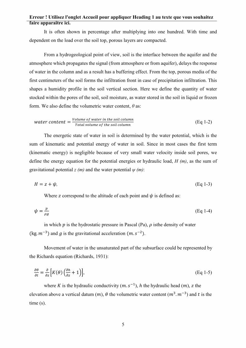
form. We also define the volumetric water content, θ as:
𝑤𝑤𝑇𝑇𝑇𝑇𝑤𝑤𝑝𝑝 𝑐𝑐𝑇𝑇𝑐𝑐𝑇𝑇𝑤𝑤𝑐𝑐𝑇𝑇 = 𝑉𝑉𝑉𝑉𝑉𝑉𝑉𝑉𝑉𝑉𝑉𝑉 𝑉𝑉𝑜𝑜 𝑤𝑤𝑝𝑝𝑇𝑇𝑉𝑉𝑤𝑤 𝑣𝑣𝑖𝑖 𝑇𝑇ℎ𝑉𝑉 𝑠𝑠𝑉𝑉𝑣𝑣𝑉𝑉 𝑝𝑝𝑉𝑉𝑉𝑉𝑉𝑉𝑉𝑉𝑖𝑖𝑇𝑇𝑉𝑉𝑇𝑇𝑝𝑝𝑉𝑉 𝑣𝑣𝑉𝑉𝑉𝑉𝑉𝑉𝑉𝑉𝑉𝑉 𝑉𝑉𝑜𝑜 𝑇𝑇ℎ𝑉𝑉 𝑠𝑠𝑉𝑉𝑣𝑣𝑉𝑉 𝑝𝑝𝑉𝑉𝑉𝑉𝑉𝑉𝑉𝑉𝑖𝑖
(Eq 1-2)
The energetic state of water in soil is determined by the water potential, which is the
sum of kinematic and potential energy of water in soil. Since in most cases the first term
(kinematic energy) is negligible because of very small water velocity inside soil pores, we
define the energy equation for the potential energies or hydraulic load, H (m), as the sum of
gravitational potential z (m) and the water potential ψ (m):
𝐻𝐻 = 𝑧𝑧 + 𝜓𝜓, (Eq 1-3)
Where 𝑧𝑧 correspond to the altitude of each point and 𝜓𝜓 is defined as:
𝜓𝜓 = 𝑝𝑝𝜌𝜌𝜌𝜌
(Eq 1-4)
in which 𝑝𝑝 is the hydrostatic pressure in Pascal (Pa), 𝜌𝜌 isthe density of water
(kg.𝑚𝑚−3) and 𝑔𝑔 is the gravitational acceleration (𝑚𝑚. 𝑝𝑝−2).
Movement of water in the unsaturated part of the subsurface could be represented by
the Richards equation (Richards, 1931):
𝜕𝜕𝜕𝜕𝜕𝜕𝑇𝑇
= 𝜕𝜕𝜕𝜕𝜕𝜕�𝐾𝐾(𝜃𝜃) �𝜕𝜕ℎ
𝜕𝜕𝜕𝜕+ 1��, (Eq 1-5)
where 𝐾𝐾 is the hydraulic conductivity (𝑚𝑚. 𝑝𝑝−1), ℎ the hydraulic head (𝑚𝑚), 𝑧𝑧 the
elevation above a vertical datum (𝑚𝑚), 𝜃𝜃 the volumetric water content (𝑚𝑚3.𝑚𝑚−3) and 𝑇𝑇 is the
time (s).
Erreur ! Utilisez l'onglet Accueil pour appliquer Heading 1 au texte que vous souhaitez faire apparaître ici.
6
Aquifers
An aquifer is a water-bearing geological unit or formation of rocks or unconsolidated
deposits that can store water and transmit it at a rate fast enough to be hydrologically significant.
There are two types of aquifers from the porosity point of view: porous and fractured aquifers.
A porous aquifer stores and transports water through pores, while a fractured rock aquifer has
limited storage capability and transports water along planar breaks. On the contrary to aquifers,
if the rate of water transmission is low, the rocks are called aquitards. From the water head point
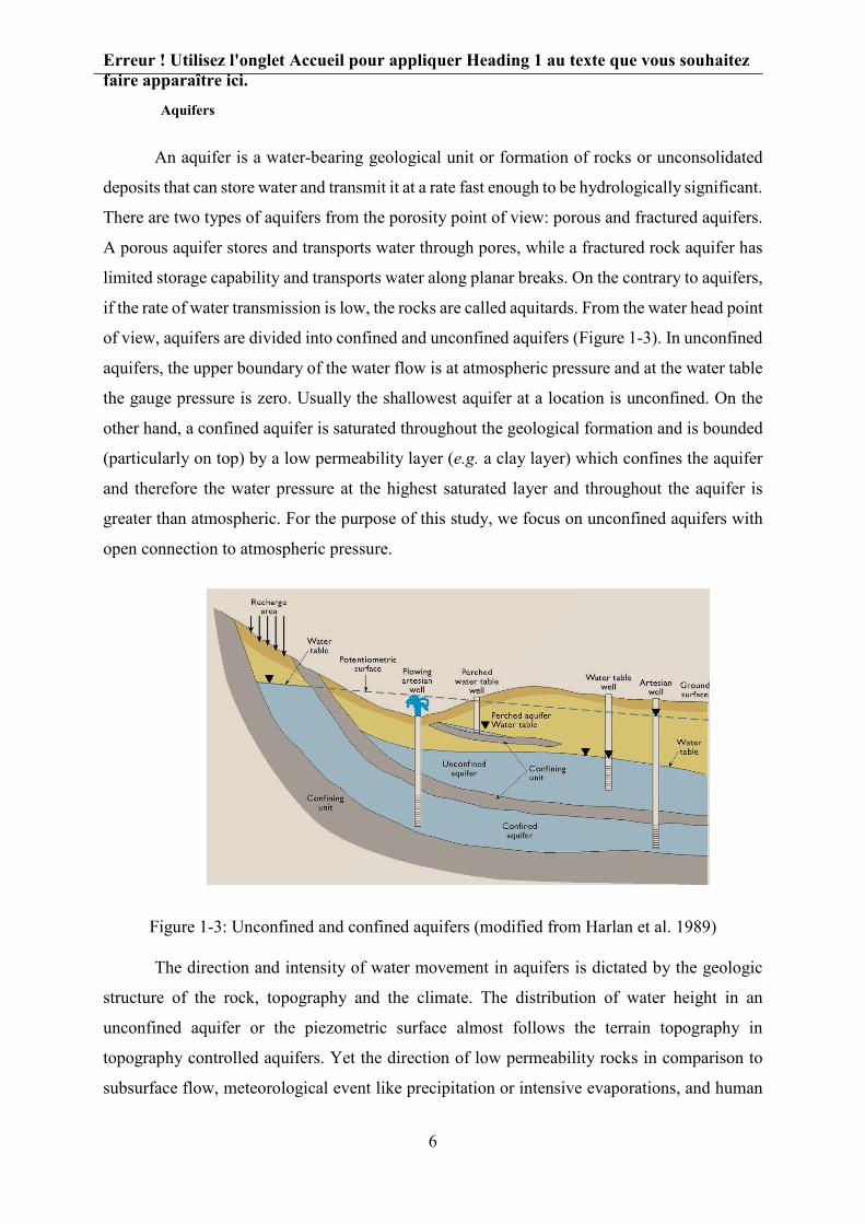
of view, aquifers are divided into confined and unconfined aquifers (Figure 1-3). In unconfined
aquifers, the upper boundary of the water flow is at atmospheric pressure and at the water table
the gauge pressure is zero. Usually the shallowest aquifer at a location is unconfined. On the
other hand, a confined aquifer is saturated throughout the geological formation and is bounded
(particularly on top) by a low permeability layer (e.g. a clay layer) which confines the aquifer
and therefore the water pressure at the highest saturated layer and throughout the aquifer is
greater than atmospheric. For the purpose of this study, we focus on unconfined aquifers with
open connection to atmospheric pressure.
Figure 1-3: Unconfined and confined aquifers (modified from Harlan et al. 1989)
The direction and intensity of water movement in aquifers is dictated by the geologic
structure of the rock, topography and the climate. The distribution of water height in an
unconfined aquifer or the piezometric surface almost follows the terrain topography in
topography controlled aquifers. Yet the direction of low permeability rocks in comparison to
subsurface flow, meteorological event like precipitation or intensive evaporations, and human

Erreur ! Utilisez l'onglet Accueil pour appliquer Heading 1 au texte que vous souhaitez faire apparaître ici.
7
exploitations of the groundwater can cause divergences of the groundwater table with respect
to the topographic surface. A steep and complex topography can generate several local flow
systems that are independent one with the others. On the contrary, in a flat topography,
groundwater flows in great distances and at high temporal scales. As a result, the groundwater
systems are rather local in steep areas and regional in flat zones. In addition to the effect of
topography and geology, climate also plays a role in groundwater flows since the aquifer
recharge rate is mainly dependent on the rate and intensity of precipitation.
Groundwater at regional to continental scales can be classified into two general types
based on geology, climate and topography (Gleeson et al., 2011a; Haitjema and Mitchell-
bruker, 2005). The first group is the recharge-controlled water tables that are expected in arid
regions with mountainous topography and high hydraulic conductivity (Figure 1-4b). In these
regions, the water table is rather deep and not in direct contact with atmosphere. In the second
group that is the topography-controlled groundwater, the water table is almost the replica of the
land surface topography. This second type of groundwater is often expected in humid regions
with rather thin soil layers and low hydraulic conductivity and is often in direct contact with
the atmosphere (Figure 1-4a).
Figure 1-4: (a) Topography-controlled water tables and (b) recharge-controlled water tables. In this figure 𝑅𝑅 is the recharge rate (m/d), 𝐿𝐿 is the distance between surface water bodies (m), 𝐾𝐾 is the hydraulic conductivity (m/d), 𝐻𝐻 is the average vertical extent of the groundwater flow
system (m) and 𝑑𝑑 is the maximum terrain rise (m). (Taken from Gleeson et al., 2011)
(a)
(b)

Erreur ! Utilisez l'onglet Accueil pour appliquer Heading 1 au texte que vous souhaitez faire apparaître ici.
8
From a broader point of view there can be three phases of interaction between the
groundwater and the atmosphere (Kollet and Maxwell, 2008): (1) the case where the Water
Table Depth (WTD) is less than 100 m, (2) the WTD is in the order of 100 m, and (3) the WTD
is far from the land surface and higher than 100 m (Figure 1-5). In the first case, the groundwater
is almost directly connected to surface condition and small changes in water table do not change
the surface variables. Similarly, in case three, small changes in the water table do not affect the
surface since linkage between groundwater and surface is weak. As for the second case, the
WTD is at a critical depth where small changes in WTD cause significant vertical redistribution
of soil moisture near the land surface.
Figure 1-5: (a) Schematic of the interconnection between GW, shallow Soil Moisture (SM) and Land Surface (LS); (b) schematic cross-section of the LS and the water table showing the
three zones of influence of groundwater (Taken from Kollet and Maxwell, 2008)
In wetlands, the water table depth is often at the range or shallower than the critical
water depth and therefore the connection between groundwater and atmosphere is strong.
Therefore, the dynamic of surface variables over the wetlands is very sensitive to both
groundwater fluxes and atmospheric conditions.

Erreur ! Utilisez l'onglet Accueil pour appliquer Heading 1 au texte que vous souhaitez faire apparaître ici.
9
1.2 Groundwater and wetlands in land surface models
1.2.1 History of land surface models
In order to simulate the exchanges of matter and energy over the surface of the Earth
integrated models named General Circulation Models (GCM) have been developed. GCMs are
generally divided into two distinct models for atmosphere and land that are sometimes coupled
to each other to simulate their interaction (e.g. Chen and Dudhia, 2001; Giorgi et al., 1993;
Pielke et al., 1997). Before introducing Land Surface Models (LSM), climatic models had fixed
boundary conditions on the land, meaning that the soil was permanently dry in arid zones of the
world and permanently wet in the tropical forests. Although it generated reasonable evaporation
fluxes, this approach did not take into account the interactions between the continental surface
and atmosphere which are essential to understand the climate. The first LSM considering the
dynamic of such interactions was that of Manabe (1969). In his model, Manabe used a
representation of the soil column which was coined later as a “bucket” model. He considered
the most effective depth of soil for interaction with atmosphere as to be the first one meter. The
entering fluxes were precipitation which infiltrates instantly (except in cases of severe storms),
and the leaving flux is the evapotranspiration with no drainage. The runoff happens when the
total soil moisture exceeds saturation. Soil is represented with only one layer with homogeneous
properties.
In Manabe’s model and in evolved versions afterwards (e.g. Deardorff, 1978), surface
parameters were treated implicitly and did not vary with time (e.g. reflective parameters of the
soil surface). Yet, in reality, these parameters can change in the presence of vegetation. As such,
optical properties of vegetation like albedo or emissivity influence the radiative balance. Plants
also play an important role in modifying atmospheric flows through their roughness. As a result,
explicit representation of vegetation was introduced to LSMs in the late 80s although Deardorff,
(1978) was among the first to propose a parametrization to calculate the energy budget, the
surface temperature, fluxes and soil humidity separately for soil and vegetation layers. Later,
more advanced processes were applied with detailed canopy and interception reservoirs,
transpiration, evaporation, extended water supply from deeper soil layers to surface and also
radiation interaction with vegetation (e.g. Sellers et al., 1986). Sellers et al. (1986) offered a
simple model for calculating the transfer of energy, mass and momentum between the
atmosphere and the vegetated surface of the Earth. In Sellers et al. (1986) model, the vegetated

Erreur ! Utilisez l'onglet Accueil pour appliquer Heading 1 au texte que vous souhaitez faire apparaître ici.
10
surface is represented as two layers: the upper one for the tree canopy, the lower one for the
annual ground cover of grasses and herbaceous species. Dickinson et al. (1993) pioneered the
Surface Vegetation Atmosphere Transfer (SVAT) models, which give the vegetation a more
direct role in determining the water and energy balance in surface by representing the stomatal
resistance for different kind of vegetation.
These evolution in models are so important that today the majority of the modeling
efforts are based on these developments. Later on, routing models were added to assure the
horizontal transfer of water on the continental surface. The routing models serve to close the
global water cycle in coupled models (land-ocean-atmosphere) and in parallel provide a tool
for validating the land surface models by permitting river flow discharge comparisons with
observations. These developments were followed by LSMs with improved representation of
subsurface hydrology, lateral soil moisture movement, evapotranspiration (Abramopoulos et
al., 1988).
1.2.2 Wetlands’ roles and functions on water cycle and climate
Wetlands are transitional environments between terrestrial and open-water aquatic
ecosystems and are among the most productive ecosystems in the world, comparable to rain
forests and coral reefs (Figure 1-6). They are transitional in terms of spatial and temporal
arrangements, for they are found between uplands and aquatic ecosystems either permanently
or seasonally. Being a buffer zone between where water enters the terrestrial system and where
it returns back to the atmosphere, wetlands are constantly changing the physiochemical
environment.
Large wetland densities often translate into lower and delayed runoff peaks, higher base
flows, and increased latent heat fluxes (Bullock and Acreman, 2010; Acreman and Holden,
2013), which directly influence climate (Bierkens and van den Hurk, 2007; Lin et al., 2016).
Dense wetland vegetation also influences the hydrology in the other direction by trapping
sediments, slowing the water flow and therefore increasing evapotranspiration and pollution
removal (Billen and Garnier, 1999; Curie et al., 2011; Dhote and Dixit, 2009; Passy et al.,
2012).
Water table fluctuations directly affect wetlands and increase or decrease soil moisture
and evapotranspiration accordingly (Dingman, 2015). It has been shown for example that

Erreur ! Utilisez l'onglet Accueil pour appliquer Heading 1 au texte que vous souhaitez faire apparaître ici.
11
without the wetland component (represented through groundwater exchanges) seasonality of
the runoff is overestimated (van den Hurk et al., 2005)
Figure 1-6: Conceptual roles functions and feedbacks affecting wetland hydrology. Dashed lines mean feedbacks and the thickness of lines emphasizes the intensity of effects or
feedbacks (not in scale)
Wetlands also affect oxygen and nutrient availability, pH and toxicity. Through these
changes, the biota may respond with massive ecosystem productivity such as: emergent plants
and concentration of animals, adapted to shallow water and dense vegetation cover.
Another aspect of wetlands role in climate is their methane (CH4) emission. Natural
wetlands (e.g. swamps and peatland) and artificial wetlands (e.g. rice paddies) in anaerobic
condition and warm climates emit methane and are the primary producer of this greenhouse
gas. Wetlands are reported to form the majority of the methane climate feedback up to 2100
(Dean et al., 2018). Methane is a powerful greenhouse gas, second only to carbon dioxide in its
importance to climate change, while concentrations of methane in the atmosphere are about 200
times lower than carbon dioxide. Generally methane has a key role in the carbon cycle both as
a sink and source (Matthews and Fung, 1987; Richey et al., 2002; Repo et al., 2007; Ringeval
et al., 2012).
Recent studies have suggested a contradictory effect of climate change over wetlands.
Wetlands with dense autotroph vegetation remove carbon dioxide (CO2) from the atmosphere
EcosystemPlants, animals and micro-organisms
Time
HydrologyDischarge,inundated area, evapo-transpiration
ClimateGeomorphology
Reduced
Oxidized
Physiochemical environment
Sedimentation, soil and water chemistry

Erreur ! Utilisez l'onglet Accueil pour appliquer Heading 1 au texte que vous souhaitez faire apparaître ici.
12
and accumulate it into the organic carbon of the soil. For this reason they have always been
accounted as one of the major Carbon sinks (Brix et al., 2001). In the meantime, anaerobic
decomposition is responsible for favoring methanogenic plants which makes wetlands the main
CH4 source. Apart from this complex carbon cycling in wetlands, some studies show that
increased temperature due to climate change may turn them into global carbon sources through
increased CH4 emission (St-Hilaire et al., 2010), while others suggest that subtropical and
temperate wetlands attenuate the effect of global warming within longer time horizons (Whiting
and Chanton, 2001).
1.2.3 Groundwater modeling as proxy for wetlands
The connecting arrows between wetland modeling and surface models is the
groundwater. Since most of the wetlands are in direct interaction with groundwater, in order to
explicitly introduce wetlands into land surface models a comprehensive groundwater
component should be added to these models.
1.2.3.1 History of recharge-discharge functions
Theoretical analysis of groundwater flow patterns under varying hydrogeological
conditions preceded actual field studies of the interaction of groundwater with surrounding
media (Tóth, 1963; Freeze and Witherspoon, 1966; Meyboom, 1966;).
The recharge-discharge function is an important but complicated part of groundwater
hydrology (Adamus and Stockwell, 1983). Groundwater discharge can maintain a high water
table in wetlands, whereas recharge to the underlying aquifers can replenish groundwater
supplies. Groundwater in local flow systems is recharged at topographic highs and discharge at
adjacent lows, while intermediate and regional scale flow systems discharge beyond adjacent
areas of low elevation of the water table. At larger scales recharge occurs between the drainage
divide and midline and discharge between the midline and the valley bottom.
Most recent advances in understanding the recharge-discharge functions have been done
through the use of a systematic approach of groundwater modeling to wetland environments.
This involves the complete description of geologic framework and hydraulic boundaries of
groundwater flow system of which wetlands are a part. The groundwater system is conceptually
and mathematically constrained by the material properties of the porous media, topography of
the water table, hydraulic potential, and flux boundaries.

Erreur ! Utilisez l'onglet Accueil pour appliquer Heading 1 au texte que vous souhaitez faire apparaître ici.
13
1.2.3.2 Groundwater in LSMs
Although groundwater models were mainly developed in late 80s notably the Modular
Three-Dimensional Finite-Difference Groundwater Flow Model (MODFLOW) by McDonald
and Harbaugh (1988), they were not integrated with other components of the continental
modeling apart from few exceptions at regional scales (e.g. Liang et al., 2003; Maxwell and
Miller, 2005). Most of the LSMs that are used for climate modeling do not explicitly include
groundwater flow processes for different reasons. Some consider that the rather thin soil column
depth used in continental modeling is not deep enough to represent hydrogeological procedures,
while others believe that the effect of aquifers on surface elements will be negligible for large
grid-sizes at large scale. The scarcity of global information on aquifer depth and properties (the
existing ones are questionable) also hinders the representation of the heterogeneity of the
groundwater flow intensity and volume. Also, LSMs encompass different non-linear mediums
of deep subsurface, shallow subsurface, soil, vegetation cover and different land cover features
which makes them global climatic bottlenecks (Desborough, 1999). This is particularly the case
when high spatial or temporal resolution is used which exponentially increases computing time
(Fuhrer et al., 2018).
The majority of the current LSMs represent the groundwater as the slow element of the
flow through drainage from the bottom of the soil. Land surface scientists have used simple
parametrization for land surface processes in regional and global climate models since they are
often used at very large scales and long temporal periods. In the beginning, these simplifications
were mainly concentrated on bucket representation of soil water content limited to field water
content capacity and also static or semi-dynamic vegetation cover without any physiological
characteristics (Carson, 1982). These simplifications did not allow a physically-based portrayal
of the groundwater interaction with surface water elements in the earth surface layer. In order
to better represent the water movements in the soil column, exchange fluxes between different
layers of soil and aquifer to the biosphere and atmosphere should be modelled through realistic
and physically-based mechanisms. Soil water movement has almost always been limited to thin
soil layer fluxes that are governed by gravitational and capillary forces and diffusion
mechanisms. Although details and complexity of processes are limited to an appropriate level
for use in General Circulation Models (GCMs), they are chosen to better model the reality at
coarse scales. In this framework the sensitivity of ground hydrology is evaluated to be
Erreur ! Utilisez l'onglet Accueil pour appliquer Heading 1 au texte que vous souhaitez faire apparaître ici.
14
maximum to land cover fractional classification including wetlands and vegetation
(Abramopoulos et al., 1988).
With the advent of computing systems, LSMs include detailed ecological processes and
lateral flows (Famiglietti and Wood, 1994; Jorgensen et al., 1989;). Yet, all interactions between
soil/vegetation/atmosphere were still considered within the first tens of centimeters of soil (with
often a static parametrization of the drainage at the bottom layer). Wetlands as the land cover
with the strongest connection with groundwater were represented only as surface water
accumulation storages with little or no interaction to subsurface water reservoirs. Few efforts
toward explicitly introducing groundwater into LSMs (within the late 90s and the early 2000s)
showed the potential to significantly shift evapotranspiration, lower the peak runoff, and
increase the base flow (e.g. Salvucci and Entekhabi, 1995; Liang et al., 2003). The role of soil
moisture and generally the water stored in land is clearer knowing that evapotranspiration from
wet soils amounts to more than half of the total solar energy absorbed by land surface (Trenberth
et al., 2009). Yeh and Eltahir (2005) developed a lumped unconfined aquifer model based on a
one-dimensional dynamic groundwater parametrization similar to Liang et al. (2003). Maxwell
and Miller (2005) coupled the Common Land Model and ParFlow as a single column model to
simulate the dynamics of surface/groundwater. Niu et al. (2007) defined an aquifer as the part
below the modeled soil column which resulted in 16% more evapotranspiration than the
scenario with a free drainage from the bottom. In a comprehensive effort to model wetlands,
Stacke and Hagemann (2012) developed a model calibrated by the wetland-affected river
discharge data to predict wetland extent. Their model calculates the wetland extent based on
balance of water flows and the slope distribution of the grid-cell.
Despite few attempts to model groundwater and wetlands at large scale, many examples
of small scale groundwater modelling exist. For simulating wetlands at small scales, the method
based on the topographic wetness index (Beven and Kirkby, 1979) is among the first and most
popular approaches. In their model, TOPMODEL, the authors assumed that topography has a
dominant effect in distributing soil moisture along the watershed. The Topographic Index (TI)
is the logarithmic ratio of the upland drainage area over the local slope for each point in space.
Soil moisture is distributed as a function of the TI value for each point, in a way that downhill
zones with flat slope have higher moisture than steep uphill areas. Therefore the possibility of
saturation is higher for zones of high TI. Within the past decades a number of terrain-based
indices have been derived and relationship between indices and hydrologic processes has been

Erreur ! Utilisez l'onglet Accueil pour appliquer Heading 1 au texte que vous souhaitez faire apparaître ici.
15
explored ( Burt and Butcher, 1986; Barling et al., 1994; Saulnier et al., 1997; Mérot et al., 2003).
These methods are generally founded on simplification of the physical processes and to include
the principal factors such as topography, climate and soil transmissivity that regulate the
system. For example Bohn et al. (2007) used the TI and the bias-correction of Saulnier and
Datin (2004) to derive the local water table depth based on mean water table depth. They then
combined it with a hydrologic and a geochemical model to estimate methane emissions over
western Siberia.
1.2.3.3 GW interaction with streams
Groundwater in its natural state is invariably moving, governed by established hydraulic
principles. Interactions between aquifer and streams can either be gaining or losing water
(Figure 1-7). In arid areas with deep water tables, it is often the river which is recharging the
groundwater through the streambed and an unsaturated zone. The groundwater/surface water
connection for the losing stream case can either be connected, disconnected or in a transitional
state (e.g. Brunner et al., 2009). In the opposite case, convergence of groundwater flows adds
water to stream either through streambed discharge or the overbank and seepage-face flows.
Here only the connected gaining streams are presented.
Generally the interaction between GW and streams occurs by subsurface flow through
infiltration/exfiltration from the saturated zones. Lateral flows often happen where the vertical
extent is limited by a horizon blocking the vertical percolation. Where such lateral flows
encounters sharp slopes or depression, in other words where seepage can occur, they contribute
to overland flow. In this context, the flow between the porous media and the free water is a
function of the head gradient between the water table and the stream. However, the larger the
scale is (in the sense of model dimensions), the less understood the interfaces (Flipo et al.,
2014).
Among the first and most important attempts to describe groundwater movement is the
Darcy law (Darcy, 1856). The flow through aquifers can be expressed by the Darcy’s law (Eq
1-6). Darcy investigated the flow of water through vertical columns of sand and established the
law for flow in sands by conducting column experiments. Darcy experiments show that the flow
rate 𝑄𝑄 (m3/s) through porous media is proportional to the head loss 𝛥𝛥ℎ (m) between two points
and inversely proportional to the length of the flow 𝐿𝐿 (m). Considering all this, the following
equation estimates the subsurface flow by introducing the hydraulic conductivity K (m/s) as the

Erreur ! Utilisez l'onglet Accueil pour appliquer Heading 1 au texte que vous souhaitez faire apparaître ici.
16
proportionality coefficient that depends on the nature of the fluid and of the medium, and A
(m2) the cross-section area:
𝑄𝑄 = 𝐾𝐾𝐾𝐾 𝛥𝛥ℎ/𝐿𝐿 . (Eq 1-6)
After Darcy, there have been several efforts to reach analytical treatments using field
theory. For example Hubbert (1940) showed that the flow depends not only on the head
potential between the two points in question and the nature of the porous medium, but also on
the property of the fluid like the viscosity and density. He also discussed the appearance of
turbulent flow in porous media based on the Reynolds number. He showed that in a totally
homogenous environment with equally-distributed precipitation and infiltration, the water table
will develop as a replica of the topography.
Rushton and Tomlinson (1979) claimed that as a result of non-linear effect, there is a
rapid increase of the flow for small head changes when the difference between aquifer and
stream water heads is small. Also the water exchange is limited to a maximum flow when the
head difference grows higher while differentiating between the flow from aquifer to stream and
vice versa.
𝑄𝑄𝑝𝑝𝑎𝑎𝑉𝑉𝑣𝑣𝑜𝑜𝑉𝑉𝑤𝑤→𝑠𝑠𝑇𝑇𝑤𝑤𝑉𝑉𝑝𝑝𝑉𝑉 = 𝐾𝐾1(1 − 𝑤𝑤−𝐾𝐾2Δℎ) (Eq 1-7)
𝑄𝑄𝑠𝑠𝑇𝑇𝑤𝑤𝑉𝑉𝑝𝑝𝑉𝑉→𝑝𝑝𝑎𝑎𝑉𝑉𝑣𝑣𝑜𝑜𝑉𝑉𝑤𝑤 = 𝐾𝐾3(𝑤𝑤−𝐾𝐾2Δℎ − 1) (Eq 1-8)
In which 𝐾𝐾3 is smaller than 𝐾𝐾1, both are a function of river width. 𝐾𝐾2 is the exponential
decay factor of the flow with respect to pressure head.
As pointed out by Rushton and Tomlinson (1979) an important point is that the
relationship between water flux and difference in head between the aquifer and river could be
different for the case when river is recharging the aquifer in comparison to the inverse situation,
in particular when disconnection occurs (gaining and losing streams: Figure 1-7). This is
because the groundwater discharges into streams both through the river bed and the surrounding
lowlands (as in return flow), but aquifer recharge by the streams is only through the river bed.

Erreur ! Utilisez l'onglet Accueil pour appliquer Heading 1 au texte que vous souhaitez faire apparaître ici.
17
Figure 1-7: Different situations in the direction of the groundwater toward streams
Prickett and Lonnquist (1971) introduced the concept of a river coefficient,
RC (m2.s-1), to represent river–aquifer interaction in regional groundwater models based on
vertical flows through an aquitard. The flux between aquifer and stream depends on the
difference between water level in the stream and the aquifer head at the streambed:
𝑄𝑄 = 𝑅𝑅𝐶𝐶 Δℎ = 𝑅𝑅𝐶𝐶 (ℎ𝑝𝑝𝑎𝑎𝑉𝑉𝑣𝑣𝑜𝑜𝑉𝑉𝑤𝑤 − ℎ𝑤𝑤𝑣𝑣𝑣𝑣𝑉𝑉𝑤𝑤). (Eq 1-9)
Herbert (1970) has also suggested a solution for aquifer-stream fluxes in confined
aquifers surrounding rather small rivers. In his study, he assumed that in such streams, the flow
leaves or enters radially and its quantity is approximated by:
𝑄𝑄 = 𝑅𝑅𝐶𝐶 Δℎ = 𝜋𝜋𝜋𝜋𝐾𝐾
𝑉𝑉𝑖𝑖� 𝑑𝑑2𝑟𝑟�Δℎ (Eq 1-10)
In which L is the length of the river (m), d is the depth of the riverbed deposits (m) and
r is the hydraulic radius of the river (m).
Miguez-macho et al. (2007) applied Darcy’s law to the mean width and elevation of all
the streams within a grid-cell to calculate the aquifer-river exchange:
𝑄𝑄 = 𝑅𝑅𝐶𝐶. �ℎ𝑝𝑝𝑎𝑎𝑉𝑉𝑣𝑣𝑜𝑜𝑉𝑉𝑤𝑤 − ℎ𝑝𝑝𝑣𝑣𝑉𝑉𝑤𝑤𝑝𝑝𝜌𝜌𝑉𝑉� (Eq 1-11)
𝑅𝑅𝐶𝐶 = 𝐾𝐾�𝑏𝑏𝑏𝑏𝑑𝑑𝑣𝑣�𝑏𝑏𝑏𝑏𝑑𝑑
𝑊𝑊� ∑𝐿𝐿 (Eq 1-12)

Erreur ! Utilisez l'onglet Accueil pour appliquer Heading 1 au texte que vous souhaitez faire apparaître ici.
18
In these formulations 𝐾𝐾�𝑏𝑏𝑉𝑉𝑣𝑣 and �̅�𝑑𝑏𝑏𝑉𝑉𝑣𝑣 are the mean hydraulic conductivity and thickness
of the river bed and W and L are the width and length of the river.
More recently, Vergnes et al. (2014) studied the groundwater over France and estimated
the river exchange from the following formula:
𝑄𝑄 = �𝑅𝑅𝐶𝐶�ℎ𝑝𝑝𝑎𝑎𝑉𝑉𝑣𝑣𝑜𝑜𝑉𝑉𝑤𝑤 − ℎ𝑤𝑤𝑣𝑣𝑣𝑣𝑉𝑉𝑤𝑤� 𝑤𝑤ℎ𝑤𝑤𝑝𝑝𝑤𝑤 ℎ𝑝𝑝𝑎𝑎𝑉𝑉𝑣𝑣𝑜𝑜𝑉𝑉𝑤𝑤 > 𝑍𝑍𝑏𝑏𝑉𝑉𝑣𝑣 𝑅𝑅𝐶𝐶(𝑍𝑍𝑏𝑏𝑉𝑉𝑣𝑣 − ℎ𝑤𝑤𝑣𝑣𝑣𝑣𝑉𝑉𝑤𝑤) 𝑤𝑤ℎ𝑤𝑤𝑝𝑝𝑤𝑤 ℎ𝑝𝑝𝑎𝑎𝑉𝑉𝑣𝑣𝑜𝑜𝑉𝑉𝑤𝑤 < 𝑍𝑍𝑏𝑏𝑉𝑉𝑣𝑣
(Eq 1-13)
in which 𝑍𝑍𝑏𝑏𝑉𝑉𝑣𝑣 is the river bed elevation and RC is calculated as below:
𝑅𝑅𝐶𝐶 = 𝜋𝜋𝐿𝐿𝜏𝜏
(Eq 1-14)
where 𝜏𝜏 is the coefficient of transfer time of water through the river bed sediment.
Pryet et al. (2015) used a similar formulation for river-aquifer exchange, adapted from
Darcy, for the horizontal flow:
𝑄𝑄 = 𝑅𝑅𝐶𝐶 �ℎ𝑝𝑝𝑎𝑎𝑉𝑉𝑣𝑣𝑜𝑜𝑉𝑉𝑤𝑤 − ℎ𝑤𝑤𝑣𝑣𝑣𝑣𝑉𝑉𝑤𝑤� = 𝑓𝑓 𝐾𝐾ℎ 𝐿𝐿 (ℎ𝑝𝑝𝑎𝑎𝑉𝑉𝑣𝑣𝑜𝑜𝑉𝑉𝑤𝑤 − ℎ𝑤𝑤𝑣𝑣𝑣𝑣𝑉𝑉𝑤𝑤) (Eq 1-15)
where 𝐾𝐾ℎ is the horizontal hydraulic conductivity and 𝑓𝑓 is an adjustable lumped parameter.
At local scales, experimental studies assuming the linear relationship between the head
gradient and the GW-SW flow may be simplistic since the friction between the flow and soil
particles is considered independent of the head gradient between water table and the stream.
The other issue is that the water table head in the aquifers surrounding streams considerably
varies in their vicinity. Yet Darcy calculation is by far the most popular formulation for
groundwater stream interactions as in famous groundwater models like MODFLOW
(McDonald and Harbaugh, 1988). The fundamental assumption of the MODFLOW is that the
head loss between aquifer and stream is limited to losses across the streambed as is shown in
Figure 1-8.

Erreur ! Utilisez l'onglet Accueil pour appliquer Heading 1 au texte que vous souhaitez faire apparaître ici.
19
Figure 1-8: The MODFLOW approach for exchange between aquifer and stream (modified from Rushton, 2007)
1.3 Objectives of the PhD thesis
In wetlands, anaerobic conditions in shallowly flooded systems decelerate the
decomposition and leads to accumulation of carbon over long periods of time. Wetlands are
vulnerable to temperature variations in the future climate. With the increased decomposition
rates (following high temperatures), they may lead to excessive carbon emissions to the
atmosphere (Watson et al., 1996). Precipitation and temperature changes result in regional
hydrological and permafrost changes that may cause loss or growth of local wetlands (Watson
et al., 2000). Additionally, sea-level rise may impact fresh and saline coastal wetland areas. In
a broader look, direct connection between groundwater and atmosphere in most wetlands allows
near-potential evapotranspiration that may lead to changes in precipitation patterns at regional
scale (Bierkens and van den Hurk, 2007). On the other hand, wetland drainage for agriculture
or other human-related purposes over floodplains and valley bottoms often decreases the
retention time during the flood season and sharpen the flow hydrograph, potentially hazardous
for human installations and water quality, although upland wetlands often tend to generate
floods (Acreman and Holden, 2013). All of these vital roles of wetlands in nature necessitate
better representation of these land features in future climate modellings in order to better
quantify their impacts and feedbacks on the environment.
Flow into aquifer
Flow into stream

Erreur ! Utilisez l'onglet Accueil pour appliquer Heading 1 au texte que vous souhaitez faire apparaître ici.
20
In this PhD work, the scientific objective is to assess the effect of wetlands on the surface
variables and climate. To obtain this objective, wetlands should be introduced in a modelling
framework and their role in interaction with other land and atmosphere features should be
defined. In order to do so a set of scientific questions is asked:
1- How can we parametrize wetlands in a land surface model in connection to
groundwater and atmosphere?
2- What is the extent and distribution of wetlands over the globe?
3- What is the impact of wetlands on environment and surface variables over a river
basin?
Most wetlands depend on groundwater resources as primarily or complementary water
source. Therefore, in order to effectively simulate wetlands dynamic, an explicit GW model
should be implemented in the land surface models. While a number of GW models have been
developed, only two examples to my knowledge are aimed and applied at fine resolution for
the global scale: Fan et al. (2013) and De Graaf et al. (2015). 2D and 3D GW modelling requires
an extensive amount of information e.g. topography, subsurface properties, high resolution
climatic variables, which are often not available at the global scale. Moreover, global climate
modelling at high temporal resolution consumes plenty of calculation time and should
necessarily be done at very coarse resolutions (~10-100 km), where small scale governing
procedures might not be valid. Therefore, to answer the first scientific question, a simple GW
distribution pattern between upland recharge zones to lowland potentially wet zones in river
basins is generated. This involves designing a scheme with the wetland component for the
climate models which describes the hydrological interactions of the wetlands with their
surrounding environment. These interactions include the fluxes of water and energy that feeds
the wetlands and also those interacting with the surface components, like evapotranspiration.
This parametrization is done within the modeling platform of ORCHIDEE land surface model,
which is the land surface element of the IPSL climate model. However, the first step in order
to simulate these processes is to distinguish between uplands and lowlands, or better said, the
recharge and discharge zones of the groundwater.
In order to define wetlands in ORCHIDEE, a parallel question is the extent and
distribution pattern of wetlands, which is the second scientific question. We decide to describe
the wetlands in ORCHIDEE model knowing that: 1) wetland fractions are input to the model
(in contrast to some models that calculate the wetland fraction themselves), and 2) wetlands are

Erreur ! Utilisez l'onglet Accueil pour appliquer Heading 1 au texte que vous souhaitez faire apparaître ici.
21
fed by the precipitation water and also the drainage from the upland fraction. To this end, there
is an essential need to develop a comprehensive global wetland map demonstrating their
geographical pattern and extent. It has been shown that lack of consistency in wetland definition
and distribution pattern leads to huge uncertainties in wetland simulations (Nakaegawa, 2012).
As a result, one of the first steps toward wetland modelling is to develop a wetland map with
uniform definition over the globe. This will help attribute wet fractions to different areas of the
world in land surface models, independently of their biogeochemical characteristics, since we
focus solely on the hydrological roles of wetlands. A conclusion in this step is that since the
wetland fractions are introduced to the model as maximum extent values, the effective wetlands
are necessarily smaller than the potential wetland extents.
At the end, using the modelling framework and the developed wetland map, simulations
are performed over a test river basin (in this case the Seine River basin). The Seine River basin
is chosen because of the substantial role of the GW in the hydrological regime and the wealth
of information on the aquifers. In this way the third and last scientific question is answered:
What is the impact of introducing wetlands on surface climatic variables? (e.g.
evapotranspiration and river flow). Then, the simulations result are compared to valid
observations available of the river flow at the downstream, evapotranspiration rates over the
basin, and also to observations of GW involving well observations and GRACE gravity
measurements.

Erreur ! Utilisez l'onglet Accueil pour appliquer Heading 1 au texte que vous souhaitez faire apparaître ici.
22

Erreur ! Utilisez l'onglet Accueil pour appliquer Heading 1 au texte que vous souhaitez faire apparaître ici.
23
Chapter 2
Development of the wetland modeling
scheme
In the first chapter, we emphasized on the importance of wetland modelling in order to
have a general view of the hydrological and biogeochemical aspects of the land surface. To this
end, the hydrological interaction at the intersection between wetlands and other hydrological
elements should be investigated. This interaction can be very complicated in different parts of
the world. Water may flow out at the ground surface from a spring or wetlands located where
the water table intersects the ground surface. On the other hand, with the exception of some
floodplains over losing aquifers, most inland wetlands are fed by the convergence of
groundwater. Inversely, floodplains are often considered as the groundwater recharge areas
during the flood season. Despite these complications, one way or the other, wetlands and
groundwater are interconnected. As a result, in order to model wetlands one important
prerequisite is to explicitly model the groundwater and its movement through wetlands.
As discussed before, groundwater is often simply represented as the drainage from the
bottom of the soil column with a large residence time. But many processes like the effect of
shallow water table on evapotranspiration and exchange of water between streams and aquifers
in both directions during different seasons are not explicitly represented in such models. In this
chapter we aim to tackle this problem by introducing a new wetlands scheme in the framework
of a land surface model.
At the first step in this chapter, the modelling platform used in this study which is the
ORCHIDEE model is explained and its different components are investigated. Then, by
emphasizing the need to describe wetlands as the transitional medium between the upland and
the streams, a separate calculation unit (soil-tile) for wetlands within the ORCHIDEE platform
is defined and its interactions with other components are designed. This section does not include

Erreur ! Utilisez l'onglet Accueil pour appliquer Heading 1 au texte que vous souhaitez faire apparaître ici.
24
the simulation results of the newly developed scheme, ORCHIDEE-WET, but it explains the
general structure, properties and interconnections of the groundwater component of this
scheme.
2.1 ORCHIDEE as the modelling platform
ORCHIDEE (ORganising Carbon and Hydrology In Dynamic Ecosystem) is the land
surface model of the Institute Pierre Simon Laplace (IPSL) Earth system model which can be
used both coupled with the atmospheric component or independently. It is a multi-collaboration
with many contributors in different countries. First efforts toward developing ORCHIDEE
started in the early 1980s with the efforts in Laboratoire de Météorologie Dynamique (LMD)
to develop a model for calculating the energy and water balance of terrestrial ecosystems (Laval
et al., 1981). Later, heterogeneity of the surface vegetation was introduced as different Plant
Functional Types (PFTs) into ORCHIDEE which enabled considering different vegetation
effects and responses to climate. In parallel to several enhancements and overhauls to improve
the coupling between the land-surface and atmosphere components, in the early 2000s, the
Dynamic Global Vegetation Model (DGVM) was introduced by merging a carbon transference
module (STOMATE) and a dynamic evolution-based vegetation module based on the LPJ
model. STOMATE describes the flow of carbon in the connected mediums of soil, plant and
atmosphere (Viovy, 1996). At this point, the first ORCHIDEE model description was published
by Krinner et al. (2005). Recently many new projects have been defined for a better
representation of the peatlands, permafrost zones, river routing scheme, soil freezing
mechanisms and many other aspects of the land surface.
Although based on natural physical relationships, each LSM like ORCHIDEE requires
basic properties and atmospheric conditions like soil type, hydraulic conductivity, surface air
temperature, air humidity, and wind speed and direction, for offline (stand-alone) configuration
in order to calculate the energy and water balances and form the vegetation and soil carbon
cycles (Figure 2-1).

Erreur ! Utilisez l'onglet Accueil pour appliquer Heading 1 au texte que vous souhaitez faire apparaître ici.
25
Figure 2-1: Schematic view of basic inputs/outputs to ORCHIDEE
2.1.1 Modular structure
ORCHIDEE land surface model is composed of three principal components namely
SECHIBA, STOMATE and DGVM.
• SECHIBA
SECHIBA (Schématisation des EChange Hydrique à l’Interface entre la Biosphère et
l’Atmosphère) is a simple physically-based model with a parametrization of the hydrologic
exchanges between the land surface (including vegetation) and the atmosphere. SECHIBA was
developed in the early 90s to be coupled with the IPSL atmospheric circulation model
(Ducoudré et al., 1993). This component describes the water vapor exchanges which is the
latent heat and also the water distribution in the vertical soil column or the hydrologic cycle.
Latent heat is composed of snow sublimation, soil evaporation, canopy transpiration and
evaporation for foliage water. Yet SECHIBA contains no parametrization of photosynthesis.
For the hydrological processes in SECHIBA, first there is a partitioning of the arriving
precipitation to infiltration and runoff, then the infiltrated water is redistributed in soil layers
and drained from the bottom end. The flowing runoff is routed into river discharge. The vertical
redistribution of water could be done by one of the two available methods in ORCHIDEE
namely; Choisnel and CWRR schemes. Choisnel scheme is a two-layer bucket model with no
drainage at the bottom (Ducharne et al., 1998; Ducoudré et al., 1993) but CWRR is a (by
Temperature
Wind
Precipitation
ORCHIDEE
Water, energy and carbon dynamics

Erreur ! Utilisez l'onglet Accueil pour appliquer Heading 1 au texte que vous souhaitez faire apparaître ici.
26
default) 11 layers (for the two meter soil) physically-based description of soil-water fluxes
through solving Richards equation with free drainage at the bottom (de Rosnay et al., 2002;
D’Orgeval et al., 2008; Campoy et al., 2013).
The water and energy exchanges on the continental surface in SECHIBA are very
dependent on the soil type and the vegetation cover. Therefore, to take into account the
heterogeneity of vegetated surfaces, a global map of vegetation cover at 5 km resolution that
provides the fraction of each vegetation type for the grid, is read by the model. This map comes
from the IGBP (International Geosphere-Biosphere Program: Belward et al., 1999) map. It is
in a higher resolution than the map read by the model (1 km). In this map, 94 vegetation classes
are provided but the rather coarse resolution of the model does not permit using all of them.
Additionally, we do not know all the parameters associated to each vegetation class.
Consequently, the vegetation types are reduced to 15 types; based on the dominant type method,
each of which is called a PFT (Plant Functional Type). They are called PFTs since they do not
represent a certain vegetation type, but they are rather the regrouped class of several species
with similar functionalities. This choice allows parametrization of the principal functionality
characteristics of plants like their height and LAI (Leaf Area Index).
Table 2-1 summarizes the characteristics of these 15 PFTs with their corresponding
parameters.

Erreur ! Utilisez l'onglet Accueil pour appliquer Heading 1 au texte que vous souhaitez faire apparaître ici.
27
Table 2-1: Summary of plant functional types (PFTs) and their characteristics (modified from Guimberteau, 2010)
Number Name h c rs k0 𝛼𝛼SW 𝛼𝛼NIR LAImin LAImax Tmin Tmax Soil tile
1 Bare soil 0 5.0 0 0.0 0 0 0 0 0 0 1
2 Tropical broadleaf evergreen 30 0.8 25 0.12 0.04 0.2 8.0 8.0 23 27 2
3 Tropical broadleaf deciduous 30 0.8 25 0.12 0.06 0.22 0 8.0 23 27 2
4 Temperate needleleaf evergreen 20 1.0 25 0.12 0.06 0.22 4.0 4.0 5 15 2
5 Temperate broadleaf deciduous 20 0.8 25 0.12 0.06 0.22 4.5 4.5 5 15 2
6 Temperate broadleaf summer green 20 0.8 25 0.25 0.06 0.22 0 4.5 5 15 2
7 Boreal needleleaf evergreen 15 1.0 25 0.12 0.06 0.22 4.0 4.0 5 15 2
8 Boreal broadleaf summer green 15 1.0 25 0.25 0.06 0.22 0 4.5 5 15 2
9 Boreal needleleaf summer green 15 0.8 25 0.25 0.06 0.22 0 4.0 5 15 2
10 C3 grass temperate 0.5 4.0 2.5 0.3 0.1 0.3 0 2.5 7 15 3
11 C4 grass 0.6 4.0 2.0 0.3 0.1 0.3 0 2.0 11 21 3
12 C3 crops 1 4.0 2.0 0.3 0.1 0.3 0 2.0 7 15 3
13 C4 crops 1 4.0 2.0 0.3 0.1 0.3 0 2.0 11 21 3
14 C3 grass tropical 0.5 4.0 2.5 0.3 0.1 0.3 0 2.5 7 15 3
15 C3 grass boreal 0.5 4.0 2.5 0.3 0.1 0.3 0 2.0 7 15 3
h: height (m); c, coefficient regarding the rooting profile (m-1); rs structural resistance (s.m-1); k0, constant used in the calculation of stomatal resistance; 𝛼𝛼SW and 𝛼𝛼NIR are the
albedo coefficients for shortwave and near infrared spectrums; LAImin and LAImax minimum and maximum leaf area index (m2.m-2); Tmin and Tmax ; the minimum and maximum
soil temperature at 50 cm depth
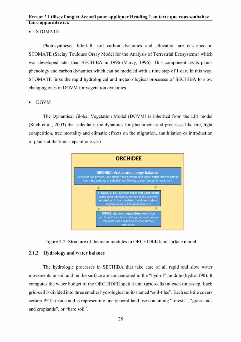
Erreur ! Utilisez l'onglet Accueil pour appliquer Heading 1 au texte que vous souhaitez faire apparaître ici.
28
• STOMATE
Photosynthesis, litterfall, soil carbon dynamics and allocation are described in
STOMATE (Saclay Toulouse Orsay Model for the Analysis of Terrestrial Ecosystems) which
was developed later than SECHIBA in 1996 (Viovy, 1996). This component treats plants
phenology and carbon dynamics which can be modeled with a time step of 1 day. In this way,
STOMATE links the rapid hydrological and meteorological processes of SECHIBA to slow
changing ones in DGVM for vegetation dynamics.
• DGVM
The Dynamical Global Vegetation Model (DGVM) is inherited from the LPJ model
(Sitch et al., 2003) that calculates the dynamics for phenomena and processes like fire, light
competition, tree mortality and climatic effects on the migration, annihilation or introduction
of plants at the time steps of one year.
Figure 2-2: Structure of the main modules in ORCHIDEE land surface model
2.1.2 Hydrology and water balance
The hydrologic processes in SECHIBA that take care of all rapid and slow water
movements in soil and on the surface are concentrated in the “hydrol” module (hydrol.f90). It
computes the water budget of the ORCHIDEE spatial unit (grid-cells) at each time-step. Each
grid-cell is divided into three smaller hydrological units named “soil-tiles”. Each soil-tile covers
certain PFTs inside and is representing one general land use containing “forests”, “grasslands
and croplands”, or “bare soil”.
SECHIBA: Water and energy balanceCalculates soil profiles, land surface temperature and water distribution at half an
hour time periods, calculating river flow at coarser temporal resolutions
STOMATE: Soil Carbon cycle and vegetation considering the vegetation type at the temporal resolution of day calculates the biomass, dead
vegetation mass, LAI and leaf albedo
DGVM: dynamic vegetation evolutioncalculates the evolution of vegetation at one year
temporal paces based on the net primary production
ORCHIDEE

Erreur ! Utilisez l'onglet Accueil pour appliquer Heading 1 au texte que vous souhaitez faire apparaître ici.
29
This module receives input variables which are the water entering the system through
precipitation (rainfall and snow). Then, it generates components of the evapotranspiration such
as transpiration, bare soil evaporation, interception loss and sublimation and calculates the
water redistribution in soil using a multi-layer scheme and Richards diffusion equation. It also
calculates the water budget in other reservoirs which are the canopy interception reservoir and
the snow pack (Ducharne, 2014). The snow pack module for a three layered snow by Wang et
al. (2013) calculates the equivalent water, snow density and its thermal conductivity. This
scheme limits the thickness of the first layer to 5 cm to better represent the diurnal change in
temperature. The second layer thickness is prescribed to 50 cm and the third layer thickness
varies with the depth of the snow.
It should be noted that the previous versions of ORCHIDEE included just a two layer
hydrology (Choisnel scheme). In the two layers version, the surface layer appeared when a
precipitation event happened and its content was drained toward the second deeper layer.
Multi-layer hydrological scheme
The multilayer module has been implemented in ORCHIDEE starting in the late
twentieth century (De Rosnay, 1999; de Rosnay et al., 2002). The default soil depth in this
scheme is two meters and again, by default, there are 11 layers on each soil column. There is a
free drainage from the bottom as a function of the hydraulic conductivity (adjustable for
reducing the drainage). The Richards equation is used in it with a source term that is derived by
combining the extended Darcy equation (Buckingham, 1907) for the non-saturated zone, using
a water content θ (m3.m-3) as in the Richards Equation, with the following continuity equation:
𝜕𝜕𝜕𝜕(𝜕𝜕,𝑇𝑇)𝜕𝜕𝑇𝑇
= −𝜕𝜕𝑎𝑎(𝜕𝜕,𝑇𝑇)𝜕𝜕𝜕𝜕
− 𝑆𝑆(𝑧𝑧, 𝑇𝑇)
𝜕𝜕𝜕𝜕(𝜕𝜕,𝑇𝑇)𝜕𝜕𝑇𝑇
= 𝜕𝜕𝜕𝜕𝜕𝜕�𝐷𝐷�𝜃𝜃(𝑧𝑧, 𝑇𝑇)� 𝜕𝜕𝜕𝜕(𝜕𝜕,𝑇𝑇)
𝜕𝜕𝜕𝜕− 𝐾𝐾(𝜃𝜃(𝑧𝑧, 𝑇𝑇))� − 𝑆𝑆(𝑧𝑧, 𝑇𝑇), (Eq 2-1)
in which 𝑇𝑇 is the time (s), 𝑧𝑧 is the depth positive toward the bottom (m), 𝑞𝑞 is the flux
field (m3.m-2.s-1), 𝑆𝑆 is the root uptake (s-1), 𝐾𝐾 is the hydraulic conductivity of the soil (m.s-1),
and 𝐷𝐷 is the hydraulic diffusivity of the soil (m2.s-1). The above equation is solved by
ORCHIDEE using a finite difference method once each 30 minutes. To discretize this
calculation, the soil column depth is divided into N nodes (this is adjustable by the user) and
each layer is labeled by i from 1 to N. The interface between each two layers is defined at the

Erreur ! Utilisez l'onglet Accueil pour appliquer Heading 1 au texte que vous souhaitez faire apparaître ici.
30
middle of each couple of nodes except for the first and the last layers, and is mathematically
described as:
ℎ1 = Δ𝑍𝑍12
(Eq 2-2)
ℎ𝑣𝑣 = [Δ𝑍𝑍𝑖𝑖+Δ𝑍𝑍𝑖𝑖+1]2
𝑓𝑓𝑇𝑇𝑝𝑝 𝑝𝑝 ∈ [2,𝑁𝑁 − 1] (Eq 2-3)
ℎ𝑁𝑁 = Δ𝑍𝑍𝑁𝑁2
(Eq 2-4)
in which Δ𝑍𝑍𝑣𝑣 is the distance between nodes 𝑝𝑝 and 𝑝𝑝 − 1 and ℎ𝑣𝑣 is the thickness of layer
𝑝𝑝. As a rule, thin layer thicknesses should be used close to interfaces where high gradients of 𝜃𝜃
are probable. This is true for the surface layer where interactions with atmosphere happen or
the bottom layer in case of non-free drainage or groundwater injection from bottom.
For the remaining procedures, 𝐾𝐾(𝜃𝜃) and 𝐷𝐷(𝜃𝜃) are calculated based on van Genuchten
(1980) with the use of prescribed saturated hydraulic conductivity for each soil texture. Soil
textures are deduced from soil maps. In ORCHIDEE, two options for soil maps are available:
Zobler and USDA. Here, the Zobler soil texture map is chosen with three classes for different
soils is used (Table 2-2). If the USDA soil texture map is used, the respective hydraulic
conductivity and diffusivity are read from another table explained in Ducharne (2014).
Table 2-2: Hydraulic parameters of the three texture classes used in ORCHIDEE: Saturation humidity, residual humidity, and hydraulic conductivity at saturation
Following the suggestion of Beven and Kirkby (1979) the saturated hydraulic
conductivity decays exponentially downward after a certain depth (𝑧𝑧𝑉𝑉𝑣𝑣𝑉𝑉) :
𝐾𝐾𝑠𝑠(𝑧𝑧) = 𝐾𝐾𝑠𝑠. min (𝑤𝑤−𝑜𝑜(𝜕𝜕−𝜕𝜕𝑙𝑙𝑖𝑖𝑙𝑙), 1), (Eq 2-5)
where 𝑓𝑓 (𝑚𝑚−1) is the e folding factor of the decaying hydraulic conductivity and is set
to 2 𝑚𝑚−1 in ORCHIDEE by default.

Erreur ! Utilisez l'onglet Accueil pour appliquer Heading 1 au texte que vous souhaitez faire apparaître ici.
31
The exponential decay of the hydraulic conductivity for the predefined three soil
textures is illustrated in Figure 2-3:
Figure 2-3: the hydraulic conductivity variations as a function of depth with an exponential decay for the three soil textures
Evaporation and water balance
In the model, total evaporation E is divided into multiple terms making a sum on bare
soil evaporation Eb, vegetation transpiration Tv, and evaporation of the intercepted water by the
plants’ leaves Ev, and the sublimation of the snow Esnow . For each grid and each vegetation
cover, the latent heat flux corresponding to evapotranspiration is calculated and then a weighted
average function is performed on them depending on the fraction of the grid covered by each
PFT leading to a single value for the latent heat flux over the grid.
𝜕𝜕𝐿𝐿𝜕𝜕𝑇𝑇
= 𝑃𝑃 − 𝐸𝐸 − 𝑅𝑅𝑇𝑇𝑉𝑉𝑇𝑇 (Eq 2-6)
𝑃𝑃 = 𝑃𝑃𝑤𝑤 + 𝑃𝑃𝑠𝑠 (Eq 2-7)
𝑅𝑅𝑇𝑇𝑉𝑉𝑇𝑇 = 𝑅𝑅𝑠𝑠𝑉𝑉𝑤𝑤𝑜𝑜𝑝𝑝𝑝𝑝𝑉𝑉 + 𝐷𝐷 (Eq 2-8)
𝐸𝐸 = 𝐸𝐸𝑏𝑏 + 𝐸𝐸𝑣𝑣 + 𝑇𝑇𝑣𝑣 + 𝐸𝐸𝑠𝑠𝑖𝑖𝑉𝑉𝑤𝑤 (Eq 2-9)
0 500 1000 1500
0
0.1
0.2
0.3
0.4
0.5
0.6
0.7
0.8
0.9
1
1.1
1.2
1.3
1.4
1.5
1.6
1.7
1.8
1.9
2
Silty SandSiltSilty clay
Silty SandSiltSilty clay
Hydraulic conductivity (mm/d)
Dept
h (m
)

Erreur ! Utilisez l'onglet Accueil pour appliquer Heading 1 au texte que vous souhaitez faire apparaître ici.
32
In these equations, 𝑊𝑊 is the sum of soil moisture (m of water), total snow mass (m of
water), intercepted water (m of water) and the water in the flow reservoirs (m of water). 𝑃𝑃 is
the total precipitation (m.s-1) summing rain (𝑃𝑃𝑤𝑤) and snow (𝑃𝑃𝑠𝑠). 𝐸𝐸 is the total evapotranspiration
(m.s-1), 𝐸𝐸𝑏𝑏 is the bare soil evaporation (m.s-1) defined for the first PFT, 𝐸𝐸𝑣𝑣 (m.s-1) and 𝑇𝑇𝑣𝑣 (m.s-
1) are the canopy interception and transpiration defined for PFT=2 to 15 and 𝐸𝐸𝑠𝑠𝑖𝑖𝑉𝑉𝑤𝑤 (m.s-1) is
the snow sublimation. 𝑅𝑅𝑇𝑇𝑉𝑉𝑇𝑇 is the total runoff containing the surface runoff, 𝑅𝑅𝑠𝑠𝑉𝑉𝑤𝑤𝑜𝑜𝑝𝑝𝑝𝑝𝑉𝑉 , and
drainage, 𝐷𝐷, all in (m.s-1).
In each time-step the calculation of water balance is pursued in the following order:
1- Filling the vegetation interception reservoir by precipitation
2- Calculating the arriving precipitation under the vegetation
3- Updating the interception reservoir after calculating 𝐸𝐸𝑣𝑣
4- Calculating 𝐸𝐸𝑏𝑏 and 𝑇𝑇𝑣𝑣 based on the availability of water in the soil column
5- Updating the soil water reservoir by calculating the total runoff and drainage
6- Calculating the potential root and soil evaporation uptake that will serve in the
calculation of water balance in the next time-step.
The general water state of each grid determines the partitioning of energy on the surface,
particularly the partitioning of radiation between latent heat flux and sensible heat flux. To
know the share of latent heat, ORCHIDEE considers the potential evaporation, which is the
flux when evaporation is not limited by the supply of water on the surface. Based on water
stress in each grid-cell, ORCHIDEE limits this potential evaporation to calculate the real
evaporation. There are different formulations to determine the potential evaporation among
which there is that of bulk evapotranspiration:
𝐸𝐸𝑝𝑝 = 𝜌𝜌𝑤𝑤𝑎𝑎
(𝑞𝑞𝑠𝑠𝑝𝑝𝑇𝑇(𝑇𝑇𝑆𝑆) − 𝑞𝑞𝑝𝑝𝑣𝑣𝑤𝑤) (Eq 2-10)
in which 𝑞𝑞𝑝𝑝𝑣𝑣𝑤𝑤 is the specific humidity of the air (kg.kg-1), 𝑞𝑞𝑠𝑠𝑝𝑝𝑇𝑇(𝑇𝑇𝑆𝑆) is the specific
humidity (kg.kg-1) of the saturated air in 𝑇𝑇𝑆𝑆 temperature (temperature of the evaporating
surface). 𝜌𝜌 is the water density (kg.m-3), and 𝑝𝑝𝑝𝑝 is the atmospheric resistance (s.m-1).
ORCHIDEE uses this formulation to calculate the total real evaporation which is the sum of all
evapotranspiration components.

Erreur ! Utilisez l'onglet Accueil pour appliquer Heading 1 au texte que vous souhaitez faire apparaître ici.
33
2.1.3 Routing
Routing schemes are components of land surface models used to close the hydrological
cycle and compute freshwater input into the ocean which determines finally ocean convection
and affects the atmospheric-ocean interactions. The freshwater flow is often calculated with
strong assumptions and simplifications for the fluvial dynamics with linear reservoirs or
constant water transfer velocity. The routing schemes simulate the flood wave delay and the
water travel time within the basin, and often estimate the water influx from permeable media
like aquifer through slow reservoirs. They still lack considering the buffer effect of water
retention in wetlands. In land surface models, routing schemes help compute hydrographs at
any grid-cell and not only at the outlet, and in this sense they can be utilized to estimate river
discharges at ungauged interim locations.
In ORCHIDEE, the routing scheme was developed in 2003 (Polcher, 2003) based on
existing routing schemes (Miller et al., 1994; Hagemann and Dumenil, 2002; Ducharne et al.,
2003). It receives the calculated surface runoff and drainage for each spatial calculation unit
and using the maps and properties of the river network, calculates the outlet stream to oceans
or inland water bodies plus the return flow to the soil column from the streams due to
oversaturation. The river basins map used for the routing in ORCHIDEE consists of more than
6000 basins of different sizes. Each grid-cell contains three flow reservoirs: stream, fast and
slow reservoirs. The stream reservoirs replace the rivers with very rapid flows in channels and
very short retention time. Fast reservoir stands for the surface runoff generated from all the
basins flowing toward to streams with slower velocity than the stream reservoir. Finally the
slow reservoir represents subsurface flows in the deeper media that are often much slower than
surface runoffs. The difference between these three reservoirs are shown using different time
constants.
𝑄𝑄𝑣𝑣(𝑇𝑇) = 1𝑇𝑇𝑖𝑖
.𝑉𝑉𝑣𝑣(𝑇𝑇), (Eq 2-11)
where 𝑉𝑉𝑣𝑣 is the water volume in reservoir i (m3.s-1) and 𝑇𝑇𝑣𝑣 is the travel time (𝑑𝑑𝑇𝑇𝑝𝑝) of a
water wave and:
𝑇𝑇𝑣𝑣 = 𝑔𝑔𝑣𝑣 .𝑘𝑘, (Eq 2-12)
in which 𝑔𝑔𝑣𝑣 is the reservoir property of reservoir i (10-3 day/km) and k is the water
retention index [km] which varies spatially based on the river slope and length.

Erreur ! Utilisez l'onglet Accueil pour appliquer Heading 1 au texte que vous souhaitez faire apparaître ici.
34
In the current version of ORCHIDEE, default values of time constants are calibrated for
the Senegal basin (Ngo-Duc et al., 2007).
In an effort to spatially estimate the base flow time constant (𝑇𝑇𝑠𝑠𝑉𝑉𝑉𝑉𝑤𝑤) in ORCHIDEE,
Schneider (2017) estimated 𝑇𝑇𝑠𝑠𝑉𝑉𝑉𝑉𝑤𝑤 at global scale based on a solution of the Boussinesq equation
for unconfined sloping aquifers. A sensitivity analysis showed that transmissivity and the
drainage density (δ) are the main uncertainty sources of 𝑇𝑇𝑠𝑠𝑉𝑉𝑉𝑉𝑤𝑤. Also, the use of spatially
distributed 𝑇𝑇𝑠𝑠𝑉𝑉𝑉𝑉𝑤𝑤 in ORCHIDEE showed a strong sensitivity of the river discharge buffer effect
to it, which worsen simulated river discharge when compared to observation.
2.1.4 Forcings
Forcings are prescribed boundary conditions to climatic models. There are different
types of these files for different components including: the soil map (for soil texture) which
defines the hydraulic properties of the flow, slope map for re-infiltration of the surface runoff,
the river network, the basins map, the vegetation map (which are finally merged into Plant
Functional Types) which dictates the plants roots uptake, LAI maps if STOMATE (the
photosynthesis component of ORCHIDEE) is not activated, and the wetland map read by
ORCHIDEE.
In offline simulations, the atmospheric information comes from meteorological data
which are themselves a combination of observed values and modelling results. All these
information are called the “atmospheric forcings” and when they are used as the boundary
condition, the modelling is called offline or forced. The forcing is imposed to the model that in
return simulates the surface fluxes. Otherwise, in online simulations, the meteorological
variables are calculate within the atmospheric model and received as inputs in ORCHIDEE.
The atmospheric forcing variables constraining SECHIBA are summarized in Table 2-3.

Erreur ! Utilisez l'onglet Accueil pour appliquer Heading 1 au texte que vous souhaitez faire apparaître ici.
35
Table 2-3: Summary of the different atmospheric variables received by SECHIBA
2.1.5 Existing wetland and groundwater parametrizations
The current ORCHIDEE version benefits from a flow reservoir structure which delays
different components of the flow particularly the slow flow (or the subsurface flow).
Consequently, the base flow is formed by the flow from the slow reservoir regulated with the
slow reservoir time-constant. This is a simple parameterization of the subsurface components.
But there has been other efforts to include floodplains and swamps.
D’Orgeval et al. (2008) designed a parametrization for the floodplains based on their
extent read from the Global Lakes and Wetlands Database (GLWD: Lehner and Döll, 2004).
They first defined a new reservoir for the water in floodplains. The river reservoir from the
upland grid-cell is first transferred to the floodplain reservoir. Then in order to compute the
floodplains area by linking its height to its volume a formulation is defined that is based on: (1)
the maximum floodplain extent 𝑆𝑆𝑉𝑉𝑝𝑝𝑚𝑚, derived by merging the wetland and floodplain classes
of GLWD, (2) the total basin area 𝑆𝑆𝐵𝐵, and (3) the height of the floodplain ℎ𝑜𝑜𝑝𝑝:
𝑆𝑆𝑜𝑜𝑝𝑝 = min �𝑆𝑆𝑉𝑉𝑝𝑝𝑚𝑚, 𝑆𝑆𝐵𝐵 �ℎ𝑓𝑓𝑓𝑓ℎ0�𝛽𝛽� (Eq 2-13)

Erreur ! Utilisez l'onglet Accueil pour appliquer Heading 1 au texte que vous souhaitez faire apparaître ici.
36
In which ℎ0=2 m and 𝛽𝛽 is set to 2 for a convex bottom shape of the floodplain. The
characteristic of the floodplains is that the evaporation is equal to 𝐸𝐸𝑝𝑝 and rainfall directly fills
the floodplain reservoir.
Ringeval et al. (2012) based their dynamic wetland formulation on the TOPMODEL
(Beven and Kirkby, 1979). Having a mean water deficit (𝐷𝐷𝑇𝑇) over one basin at time t, the
distributed deficit 𝑑𝑑𝑣𝑣,𝑇𝑇 for each gird-cell can be written as:
𝑑𝑑𝑣𝑣,𝑇𝑇 = 𝐷𝐷𝑇𝑇 + 𝑀𝑀(𝜆𝜆𝑉𝑉 − 𝜆𝜆𝑣𝑣), (Eq 2-14)
in which 𝜆𝜆𝑣𝑣 is the topographic index in the grid-cell i, 𝜆𝜆𝑉𝑉 is the mean topographic index
in the basin, and M is a parameter. Then a threshold 𝜆𝜆𝑇𝑇ℎ is defined so that all the pixels with
higher topographic indices than 𝜆𝜆𝑇𝑇ℎ have zero deficit (almost saturated). The mean basin water
deficit is calculated as a proportion of the soil moisture in ORCHIDEE (𝜔𝜔):
𝐷𝐷𝑇𝑇 = [(𝜔𝜔𝑉𝑉𝑝𝑝𝑚𝑚 − 𝜔𝜔𝑉𝑉𝑣𝑣𝑖𝑖) − 𝜔𝜔𝑉𝑉𝑣𝑣𝑖𝑖] ℎ𝑠𝑠𝑉𝑉𝑣𝑣𝑉𝑉 (Eq 2-15)
where ℎ𝑠𝑠𝑉𝑉𝑣𝑣𝑉𝑉 is the ORCHIDEE soil depth. There is also a parametrization of effective
wetland fraction based on the amount of frozen excess water. Finally, in saturated or partly
saturated grid-cells, the evaporation is set equal to its potential rate for the saturated areas
(increases the total evaporation).
2.2 ORCHIDEE-WET
To model wetlands, groundwater components of the models should be activated as well
as the surface water components, since most wetlands are fed from aquifers at different scales.
Groundwater models intend to represent basic features of the groundwater system through a
mathematical formulation. This requires understanding the physical, chemical and biological
laws governing the groundwater system. Such models are physically based models derived from
the Darcy’s law and the conservation of mass law. In simplified wetland modeling, wetland
components receive water from upland drainage and sometimes from the river overflows.
In its current form, ORCHIDEE, involves a simple parametrization of different
components of the flow, including the groundwater through the time constant for slow reservoir.
The effort here in ORCHIDEE-WET is to include a second parametrization for the hillslope
hydrology and wetlands, by defining the wetland soil-tile.

Erreur ! Utilisez l'onglet Accueil pour appliquer Heading 1 au texte que vous souhaitez faire apparaître ici.
37
Wetlands are very complicated land features with interwoven connections to vegetation,
surface streams, and aquifers. To be able to simulate them, accurate information on their
geographic distribution, soil texture, river exchange zones, and widths are required. On the
other hand, land surface models often face the problem of calculation time and are therefore
up-scaled: most of LSMs calculate the water budget in grid-cells of average width 50 km. At
these resolutions, many land features are averaged for simplicity. However, sub-grid
parameterization can sometimes help representing fluxes of water related to processes such as
infiltration and evapotranspiration in particular land types.
2.2.1 Simplified wetland element
To introduce complicated land features such as the hillslope hydrology to a physically
based land surface model like ORCHIDEE, many simplifications are required for the physics
and the geometry of the basins. The first determining factor is the resolution of the model (by
default 0.5°) which necessitates ignoring sub-grid heterogeneities and small scale processes like
second order effects of small elevation differences near the streams and curvature of the river.
Another important simplification is to consider the soil depth limited to a few meters. The
specific simplifications for wetlands concern their geographical positioning with regards to
uplands. In this new scheme the grid-cell is divided into two adjacent tiles of uplands and
lowlands. In a grid-cell of 0.5° (~ 50 km) there is often tens of small valleys that lessens the
distance between lowlands and uplands. The interaction between the lowland (wetland) fraction
and the stream is limited to a built up water table in this fraction of the grid-cell. All these
simplifications, in addition to ORCHIDEE-WET reservoirs and fluxes are represented in Figure
2-4.
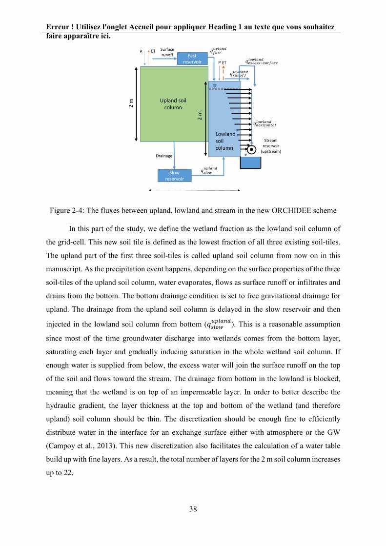
Erreur ! Utilisez l'onglet Accueil pour appliquer Heading 1 au texte que vous souhaitez faire apparaître ici.
38
Figure 2-4: The fluxes between upland, lowland and stream in the new ORCHIDEE scheme
In this part of the study, we define the wetland fraction as the lowland soil column of
the grid-cell. This new soil tile is defined as the lowest fraction of all three existing soil-tiles.
The upland part of the first three soil-tiles is called upland soil column from now on in this
manuscript. As the precipitation event happens, depending on the surface properties of the three
soil-tiles of the upland soil column, water evaporates, flows as surface runoff or infiltrates and
drains from the bottom. The bottom drainage condition is set to free gravitational drainage for
upland. The drainage from the upland soil column is delayed in the slow reservoir and then
injected in the lowland soil column from bottom (𝑞𝑞𝑠𝑠𝑉𝑉𝑉𝑉𝑤𝑤𝑉𝑉𝑝𝑝𝑉𝑉𝑝𝑝𝑖𝑖𝑣𝑣). This is a reasonable assumption
since most of the time groundwater discharge into wetlands comes from the bottom layer,
saturating each layer and gradually inducing saturation in the whole wetland soil column. If
enough water is supplied from below, the excess water will join the surface runoff on the top
of the soil and flows toward the stream. The drainage from bottom in the lowland is blocked,
meaning that the wetland is on top of an impermeable layer. In order to better describe the
hydraulic gradient, the layer thickness at the top and bottom of the wetland (and therefore
upland) soil column should be thin. The discretization should be enough fine to efficiently
distribute water in the interface for an exchange surface either with atmosphere or the GW
(Campoy et al., 2013). This new discretization also facilitates the calculation of a water table
build up with fine layers. As a result, the total number of layers for the 2 m soil column increases
up to 22.
Stream reservoir
(upstream)
Lowland soil column
Upland soil column2
m
2 m
Surface runoff Fast
reservoir
Slow reservoir
Drainage
P ET
P ET

Erreur ! Utilisez l'onglet Accueil pour appliquer Heading 1 au texte que vous souhaitez faire apparaître ici.
39
The saturated soil layers in the lowland fraction also often leads to building up a water
table in this fraction which will exchange water horizontally with the nearby stream. The water
exchange rate between the wetlands and the streams depends on the hydraulic conductivity of
the soil layers and the water head difference between the water table and the stream. Here, the
stream level is assumed to be equal to that of the bottom of the wetland soil column so that the
maximum water head difference between wetlands and the stream is limited to the depth of the
soil column. Since there is an assumption for the exponential decrease of the hydraulic
conductivity with depth in ORCHIDEE (Eq 2-5), the flow from the top layers of the aquifer is
more intense than from the bottom layers.
2.2.2 Water balance in wetlands
The water balance in the new wetland soil column is composed of two incoming and
three outgoing flow components (Figure 2-4). The entering flows are the sum of precipitation
infiltration on the top layer of the wetlands and the flow coming from the slow reservoir
(𝑞𝑞𝑠𝑠𝑉𝑉𝑉𝑉𝑤𝑤𝑉𝑉𝑝𝑝𝑉𝑉𝑝𝑝𝑖𝑖𝑣𝑣). The exiting components are the horizontal flow from the water table to the stream
(𝑞𝑞ℎ𝑉𝑉𝑤𝑤𝑣𝑣𝜕𝜕𝑉𝑉𝑖𝑖𝑇𝑇𝑝𝑝𝑉𝑉𝑉𝑉𝑉𝑉𝑤𝑤𝑉𝑉𝑝𝑝𝑖𝑖𝑣𝑣 ), the evapotranspiration from the surface, and the excess water from the top of the
wetland soil column in case of oversaturation (𝑞𝑞𝑉𝑉𝑚𝑚𝑝𝑝𝑉𝑉𝑠𝑠𝑠𝑠−𝑠𝑠𝑉𝑉𝑤𝑤𝑜𝑜𝑝𝑝𝑝𝑝𝑉𝑉𝑉𝑉𝑉𝑉𝑤𝑤𝑉𝑉𝑝𝑝𝑖𝑖𝑣𝑣 ) in the whole wetland fraction.
The sum of the runoff from upland and lowland soil columns (𝑞𝑞𝑜𝑜𝑝𝑝𝑠𝑠𝑇𝑇𝑉𝑉𝑝𝑝𝑉𝑉𝑝𝑝𝑖𝑖𝑣𝑣 + 𝑞𝑞𝑤𝑤𝑉𝑉𝑖𝑖𝑉𝑉𝑜𝑜𝑜𝑜𝑉𝑉𝑉𝑉𝑤𝑤𝑉𝑉𝑝𝑝𝑖𝑖𝑣𝑣) is a
bypassing flow without any interaction with the wetland soil column. The difference between
these entering and exiting flows equals the stock of water in the soil column.
When the wetland soil column is completely saturated, all the converging groundwater
which is injected from the bottom is directly transferred to the excess water flow component
and the effect of the wetland component is bypassed. This case often happens when the wetland
fraction is very small (and the upland is large) so that the large amount of slow-flow from the
slow-reservoir rapidly fills the wetland soil column.
The water table is formed when the deepest soil layer becomes saturated. At each time-
step, the entering flux from the bottom to the lowland is redistributed in the soil column and if
the balance between the entering flux, the outgoing flux to the river, and the evapotranspiration
is positive, the water table builds up from bottom, approaching the surface. In other words, the
water table depth is the depth of the nearest saturated layer to the surface. The flow from the

Erreur ! Utilisez l'onglet Accueil pour appliquer Heading 1 au texte que vous souhaitez faire apparaître ici.
40
water table to the river or the base flow (𝑄𝑄𝑏𝑏𝑝𝑝𝑠𝑠𝑉𝑉[𝑚𝑚3. 𝑝𝑝−1] is calculated from the equation below
which is the solution of Brutsaert (2008) [page 401] based on the Darcy’s law :
𝑞𝑞𝑉𝑉𝑉𝑉𝑤𝑤𝑉𝑉𝑝𝑝𝑖𝑖𝑣𝑣ℎ𝑉𝑉𝑤𝑤𝑣𝑣𝜕𝜕𝑉𝑉𝑖𝑖𝑇𝑇𝑝𝑝𝑉𝑉 = 𝑄𝑄𝑏𝑏𝑝𝑝𝑠𝑠𝑉𝑉 = 𝐸𝐸𝐸𝐸. (𝐿𝐿.∆𝑧𝑧).𝐾𝐾. ∆𝜕𝜕𝐵𝐵
, (Eq 2-16)
𝑄𝑄𝑏𝑏𝑝𝑝𝑠𝑠𝑉𝑉 = 𝐿𝐿.𝐸𝐸𝐸𝐸.𝑇𝑇(𝑧𝑧). ∆𝜕𝜕𝐵𝐵
, (Eq 2-17)
𝐵𝐵 = 12𝛿𝛿
, (Eq 2-18)
where 𝐿𝐿 is the length of the model grid-cell (𝑚𝑚), 𝐸𝐸𝐸𝐸 is the exchange factor of the flow which
accounts for variation of hydraulic conductivity along the horizontal direction, water table
shape, and other characteristics of the interaction surfaces. 𝑇𝑇 (𝑚𝑚2. 𝑝𝑝−1) is the transmissivity that
depends on the thickness of the saturated surface (∆𝑧𝑧) and hydraulic conductivity. ∆𝜕𝜕𝐵𝐵
is the
head gradient which depends on ∆𝑧𝑧 (𝑚𝑚), the head difference between the aquifer and the
stream, and 𝐵𝐵 mean aquifer breadth in lowland tile (𝑚𝑚). By default, the value of EF is 𝜋𝜋2
4~2.5
which is numerical factor based on the water table shape (Brutsaert, 2008). Since other factors
are also effective in this formulation (like the variation of hydraulic conductivity in the
horizontal direction), EF is finally larger than 2.5.
This equation is based on Darcy formula (Sect. 1.2.3), where the head gradient is a
function of 𝛿𝛿 the drainage density [km-1] in the grid-cell and the water level. 𝐵𝐵 is defined as half
of the inverse drainage density since each aquifer is bounded by two rivers at least.
Figure 2-5 : The schematic view of the lowland soil-tile and its interaction with the stream (credit: Agnès Ducharne)

Erreur ! Utilisez l'onglet Accueil pour appliquer Heading 1 au texte que vous souhaitez faire apparaître ici.
41
The formulation is useful for large scale hydrological modeling since it is based on large
scale input data like the map of the drainage density and coarse scale hydraulic conductivity
data (for calculating the transmissivity).
2.2.3 Distributed wetland characteristics
All wetlands in ORCHIDEE-WET are defined using identical characteristics. In other
words, there is no difference between different classes of wetlands in the hydrological modeling
scheme. In each cell, wetlands are often assumed to be located along streams, with direct
interaction. Also, implicitly, wetlands are assumed to be in the lowland fraction of the pixel
with streams being the lowest parts. As a result, the water table depth in wetland fraction is not
the mean value along the cell but rather the water table depth in the valleys.
To introduce the wetlands fraction to each grid-cell, a newly developed wetland map,
the CW-WTD map (Chapter 3) is used. The wetland pixels of resolution 500 m in CW-WTD
are aggregated to 0.5° and used as a forcing for wetland soil-tile extent.
Prescribed wetland fractions are partitioned among all 13 PFTs based on their area. For
example if the wetland fraction of one cell is 0.2, 20% of each of the soil tiles 1 to 3 is transferred
to soil-tile 4 which is the wetland. In this way the partitioning of PFTs in upland and lowland
soil column are similar. This might not be always a correct assumption. Depending on the
climatic condition, wetlands may form over lowland grasslands or tropical forests, and
sometimes over the bare soil, although vegetation is itself an indicator of wetland existence.
But in absence of complementary information on the vegetation cover in wetlands (high
resolution land-cover maps), this assumption seems to be reasonable.
Although the elevation difference between streams and surrounding wetlands can vary
up to tens of meters, by assuming a soil column with a few meters depth, we limit this elevation
difference and therefore the head difference. This is a reasonable assumption since if the water
table depth is deeper than the few meters depth soil column (with regards to our definition in
chapter 3, 20 cm), the potential lowland fraction could not be considered a wetland, because
the interaction with atmosphere is very limited (Campoy et al., 2013). Yet here the saturated
layer thickness is assumed to be less than two meters which is not always the case.
The saturated hydraulic conductivity in the wetland component is identical to that in the
other parts of the grid-cell based on the hydraulic conductivity derived from the soil texture

Erreur ! Utilisez l'onglet Accueil pour appliquer Heading 1 au texte que vous souhaitez faire apparaître ici.
42
map. This conductivity, however, decreases exponentially with depth as a function of the
decaying factor as in the uplands (Eq 2-5), but the bottom hydraulic conductivity is set to zero
for the wetland. It should be noted that in calculating the base flow from the wetland soil-tile
the horizontal hydraulic conductivity should be used since the flow is lateral.
2.3 Conclusion
Introducing the groundwater and wetland components in land surface models is very
challenging. One reason is that there is not enough information on the location of aquifers, their
depth, their 3D geometry and also their hydrodynamic properties. However, at the first step, all
aquifers are assumed to inherit the same characteristics like connection to streams and the
maximum depth of the aquifer. In our modelling platform (ORCHIDEE), the water exchange
inside one grid-cell of 0.5° is through a sub-grid scale mechanism between the upland (non-
wetland), lowland (wetland) and the stream.
Although this representation is very simple, it contains all of the fluxes from
groundwater to surface or atmosphere water, along with the return flows and re-infiltrations. It
consists of defining a new soil-tile in each grid-cell which receives water not only from the
infiltration of the incoming precipitation, but also from converging groundwater (the water in
slow reservoir) which is injected from the bottom of this soil-tile. Adding this new component
is the first step toward introducing more complicated subsurface processes within the soil
column. On the other hand, the simplistic definition of fluxes may lead to variables that are not
physically comparable to observed values. For example, we define the wetland component to
have zero drainage from bottom. Additionally the aquifer has a depth of few meters with the
bottom layer at river level. However, in reality, a portion of the exchange between streams and
aquifers happen at the river beds. This is true also for the elevation difference between wetlands
and streams which is assumed to be a few meters.
As noted before, ORCHIDEE (in its original format) includes a simple groundwater
parametrization through linear reservoirs of the routing scheme (slow reservoir). Also, there are
representations of the floodplains and swamps through defining the floodplain reservoir in the
routing scheme (D’Orgeval et al., 2008). Yet, the efforts here in ORCHIDEE-WET is a
complementary initiative to include the hillslope hydrological in the hydrology module.

Erreur ! Utilisez l'onglet Accueil pour appliquer Heading 1 au texte que vous souhaitez faire apparaître ici.
43
The most important simplification is the depth of the soil column both in upland and
lowland. Aquifers are not represented in the uplands which is not always true. Most of the time
the aquifers are deeper and thicker than a few meters, but the fluctuation of the water table is
often within a few meters of the aquifer. Another limitation of this representation is that the
lowland fraction is not dynamic and is fixed. Also, the interaction between the aquifer and the
streams is always assumed to be in the form of a gaining stream. Although hydrological systems
vary spatially and temporally, this assumption is sometimes true for mid-latitude zones with
considerable annual precipitation and over the plains. In arid zones with deep water tables,
rivers are often losing water to recharge the groundwater, knowing that the wetland fraction is
very small in such areas.
All in all, introducing the groundwater processes and wetlands in ORCHIDEE is a noble
advance toward the integration of the hydrological processes, including the groundwater
interactions.

Erreur ! Utilisez l'onglet Accueil pour appliquer Heading 1 au texte que vous souhaitez faire apparaître ici.
44

Erreur ! Utilisez l'onglet Accueil pour appliquer Heading 1 au texte que vous souhaitez faire apparaître ici.
45
Chapter 3
Development of a global wetland map
In order to quantify the effects of wetlands on hydrology, an important step is to quantify
and spatially locate zones with potential wetness over the globe. This will also help, in further
steps, to assess the role of wetlands in climate in particular with respect to climate change and
human activities. There has been several efforts to map wetlands globally which showed
wetland extent to cover between 3% and 21% of the total land surface area (e.g. Matthews and
Fung, 1987; Finlayson et al., 1999; Lehner and Döll, 2004; Prigent et al., 2007; Hu et al., 2017).
This large inconsistency is mainly derived by two factors. The first one is the lack of consistent
and unique definition for wetlands among scientists. The second limitation is that groundwater
driven and non-inundated wetlands are often overlooked. In this PhD project, one of the
important scientific questions was the global wetland extent and spatial distribution. Having a
global wetland map, potential wet fractions can be attributed to grid-cells of the general
circulation models. The wetland fraction in each grid-cell could be assumed as the most lowland
part of the land in that grid-cell, as discussed in chapter 2, where water accumulates, and if the
situation is favorable wetlands are formed.
In this work, a number of wetland products has been used and for one of them (the ESA-
CCI land cover product), a choice was done in the selection of the land cover classes with
wetland characterizations. In the Regularly Flooded Wetlands (RFW) class, we focused on
zones with almost permanent inundation. Therefore, the land cover class “cropland irrigated or
post-flooding” is not considered as a regularly flooded zone, since most irrigated croplands are
seasonally inundated and post flooding zones are often only flooded during the wet season of
the year. As a result of this choice, there have been some differences between the ESA-CCI

Erreur ! Utilisez l'onglet Accueil pour appliquer Heading 1 au texte que vous souhaitez faire apparaître ici.
46
derived wetland map and other products. Such differences are mostly explained by the
exclusion of the “cropland irrigated or post-flooding” class. Also, since the water body class
was obtained using the microwave data (and not only the optical solar data), some remarks on
the inefficiency of the ESA-CCI land cover because of only using the visible range products, is
false.
The results of the efforts to develop a global wetland map is published as a journal article
in Earth System Science Data (ESSD), available in https://www.earth-syst-sci-
data.net/11/189/2019/essd-11-189-2019.pdf. Some details about the geographic information
system settings that we used and definition are explained in annex A. Some remarks on the
usage of hydraulic conductivity maps to derive the transmissivity is explained in annex B. The
supplementary information to this journal article is enclosed in annex C.
3.1 Introduction
Wetlands are valuable ecosystems with a key role in the carbon, water and energy cycles
(Matthews and Fung, 1987; Richey et al., 2002; Repo et al., 2007; Ringeval et al., 2012). Water
retention in wetlands leads to lower and delayed runoff peaks, higher base flows, and
evapotranspiration which directly influence climate (Bierkens and van den Hurk, 2007; Lin et
al., 2016). Wetlands also serve to purify pollutions from natural and human sources, thus
maintaining clean and sustainable water for ecosystems (Billen and Garnier, 1999; Dhote and
Dixit, 2009; Curie et al., 2011; Passy et al., 2012). Despite their widely recognized importance,
no consensus exists on wetland definitions and their respective areal extents among the
reviewed literature (Table 3-1). Based on tens of definitions, the extents range from regions
with relatively shallow water tables ( National Research Council, 1995; Kutcher, 2008; Ramsar,
2009) to areas with permanent inundation such as lakes (lacustrine wetlands) with depths of
several meters. The reasons for this ambiguity are a diversity of scientific points of views as
well as the complexity of classification in transitional land features and temporally varying land
features under human influences ( Mialon et al., 2005; Papa et al., 2010; Ringeval et al., 2011;
Sterling et al., 2013; Hu et al., 2017; Mizuochi et al., 2017). Another for these limitations in
definition and detection of wetlands is the diversity of the satellite observations. This is shown
for example in Aires et al. (2018) for the differences in GIEMS-D3 (Aires et al., 2017), Landsat
images and GLWD.

Erreur ! Utilisez l'onglet Accueil pour appliquer Heading 1 au texte que vous souhaitez faire apparaître ici.
47
Table 3-1: Summary of water body, wetland and related proxy maps and datasets from the literature. The wet fractions indicated in % in the last column are those indicated in the reference paper or data
description for each study.
Name and reference Resolution Type of acquisition Wetland extent
(million km2)
% of the land*
Maltby and Turner (1983) - Based on Russian geographical studies 8.6 6.6%
Matthews and Fung (1987) 1 degree Development from soil, vegetation and inundation maps 5.3† 4.0%
Mitsch and Gosselink (2000) Polygons Gross estimates, Combination of
estimates and maps ~20† ~15.3%
GLWD-3 Lehner and Döll (2004) 30 arc-sec ~1km Compilation of
national/international maps 8.3 - 10.2‡ 6.2 - 7.6%
GLC2000 Bartholomé and Belward (2005)
1 km at Equator SPOT vegetation mission satellite observations 4.9 3.4%
GIEMS Prigent et al. (2007) 0.25° ~25km Multi sensor: AVHRR, SSM/I,
Scatterometer ERS 2.1 – 5.9 1.4 – 4%
Fan et al. (2013) 30 arc-sec ~1km Groundwater modelling ~19.3† ~17% GLOWABO Verpoorter et al. (2014)
Shapefiles of lakes larger than 0.002 km2
Satellite imagery: Landsat and SRTM topography 5 3.7%
SWAMPS Schroeder et al. (2015) 25 km
Modeling using multi sensor info: SSM/I, SSM/S, QuikSCAT, ASCAT
7.7 – 12.5§ 5.2 – 8.5%
ESA-CCI land cover Bontemps et al. (2012) 10 arc-sec ~300m Multi sensor: SPOT vegetation,
MERIS products 6.1 4.7%
GIEMS-D15 Fluet-Chouinard et al. (2015)
15 arc-sec ~460m Multi-sensor: SSM/I, ERS-1, AVHRR, Downscaled from a 0.25° wetland map
6.5 – 17.3 5.0 - 13.2%
G3WBM Yamazaki et al. (2015) 3 arc-sec ~90m Satellite imagery: Landsat 3.2 2.5%
JRC Surface water Pekel et al. (2016) 1 arc-sec ~30m
Satellite imagery: Landsat, including maximum water extent and interannual occurrence
2.8 – 4.4 2.1 - 3.4%
HydroLAKES Messager et al. (2016)
Shapefiles of lakes larger than 0.1 km2
Multiple inventory compilation including Canadian hydrographic dataset and SWBD
2.7 1.8%
Hu et al. (2017) 1 km Development based on topographic wetness index and land-cover 29.8¶ 22.5%
Poulter et al. (2017) 0.5° ~50km Merging SWAMPS and GLWD-3 10.5 7.1%
It should be noted that the wetland extent in some of these datasets like GIEMS are dynamic throughout the year. * Percentages are those from the corresponding journal article or book. If no mention of percentage coverage exists, the value is calculated by dividing the wetland area by the land surface area excluding Antarctica, the glaciated Greenland and lakes. † Excluding Caspian sea and large lakes ‡ Excluding Antarctica, glaciated Greenland, lakes and Caspian sea. Additionally the range in GLWD is different based on interpretation of fractional wetlands. § Excluding large water bodies ¶ Including the Caspian sea

Erreur ! Utilisez l'onglet Accueil pour appliquer Heading 1 au texte que vous souhaitez faire apparaître ici.
48
The first global wetland maps were developed based on compilation of regional archives
and estimates. Matthews and Fung (1987) developed a 1° resolution wetland map based on
vegetation, soil properties and inundation fractions that covered ca. 4% of the land. Finlayson
et al. (1999) based their estimates on surveys and the Ramsar global inventory in which
wetlands cover 9.7% of the land area. Later, the Global Lakes and Wetlands Database (GLWD)
was developed at 30 arc-sec resolution (~1 km at the Equator) by compiling several national
and regional wetland maps with a global cover of 6.9% of land area, excluding Antarctica and
glaciated lands (Lehner and Döll, 2004). Since satellite imagery permits homogeneous
observation of land characteristics, this method has been favored for mapping of water-related
features in recent decades. Satellite imagery at visible wavelengths reports that 1.6 to 2.3% of
Earth’s land is permanently under water (Verpoorter et al., 2014; Feng et al., 2015; Yamazaki
et al., 2015; Pekel et al., 2016) but with large disagreements (Nakaegawa, 2012), and
inundations under densely vegetated and clouded areas are often missed (Lang and McCarty,
2009). Longer wavelengths in the microwave band (e.g., L and C bands) penetrate better
through the cloud and vegetation layer and supply dynamic observations of inundated zones,
usually with a trade-off between high resolution with a low revisit rate or domain extent (Li and
Chen, 2005; Hess et al., 2015) and coarse resolution with a high revisit rate up to global
coverage (Prigent et al., 2007; Papa et al., 2010; Schroeder et al., 2015; Parrens et al., 2017).
Recent progress has been achieved by downscaling or correcting the latter products using
higher-resolution information. Fluet-Chouinard et al., (2015) developed the global inundation
product GIEMS-D15 by downscaling the 0.25° multi-satellite wetland fractions of Prigent et
al. (2007) using 15 arc-sec topography, with a global long-term maximum inundation fraction
of 13%. Poulter et al. (2017) corrected the wetland fractions of the Surface WAter Microwave
Product Series (SWAMPS: Schroeder et al., 2015) by merging them with those obtained at 30
arc-sec from GLWD.
However, regardless of the wavelengths, wetlands derived from satellite imagery almost
always represent inundated areas and overlook other types of wetlands where soil moisture is
high but the surface is not inundated (Maxwell and Kollet, 2008; Lo and Famiglietti, 2011;
Wang et al., 2018). The method most frequently used to delineate these wetlands is water table
depth (WTD) modelling. Direct groundwater (GW) modelling (e.g., Miguez-Macho and Fan,
2012) requires in-depth knowledge of the physics of water movement, topography at a
sufficiently high resolution, climate variables, subsurface characteristics and observational
constraints (Fan et al., 2013; De Graaf et al., 2015). Simplified GW models based on the

Erreur ! Utilisez l'onglet Accueil pour appliquer Heading 1 au texte que vous souhaitez faire apparaître ici.
49
topographic index (TI) of TOPMODEL (Beven and Kirkby, 1979) require less extensive input,
and they have also been used to map wetlands (e.g., Gedney and Cox, 2003). Using the
topography, TI can be calculated as follows:
𝑇𝑇𝑇𝑇 = 𝑇𝑇𝑐𝑐 � 𝑝𝑝𝑇𝑇𝑝𝑝𝑖𝑖 (𝛽𝛽)
�, (Eq 3-1)
where a is the drainage area per unit contour length (m), and 𝑇𝑇𝑇𝑇𝑐𝑐 (𝛽𝛽) is the local slope
at the desired pixel. The TI index is often presented as a wetness index (Wolock and McCabe,
1995; Sørensen et al., 2006) because high values are found over flat regions with large drainage
areas corresponding to a high propensity for saturation. Other environmental characteristics
such as climate and soil or underground properties can also be used in the TI formulation to
detect wetlands in areas where topography is not the primary driver of the water budget, such
as wetlands in uplands and over clayey soils or thin active layers in the permafrost region (e.g.,
Saulnier et al., 1997; Mérot et al., 2003; Hu et al., 2017).
A major challenge in identification of wetlands through GW modelling is the definition
of thresholds on TI or WTD for separation of wetland from non-wetland areas. At the local
scale the thresholds are often calibrated to reproduce the extent of documented wetlands in a
certain region and are subsequently extrapolated for larger domains. This strategy was proven
successful at the basin scale (e.g., Curie et al., 2007), but it has been shown to be ineffective at
larger scales because it is not possible to uniquely link TI values to soil saturation levels across
different landforms and climates (Marthews et al., 2015). Hu et al. (2017) produced a global
wetland map by calibrating TI thresholds for every large basin of the world based on land cover
maps, as pioneered over France due to independent TI threshold calibration in 22 hydro-
ecoregions using soil type datasets (Berthier et al., 2014). Uniform WTD thresholds (0 cm for
inundated areas and 25 cm for wetlands) are applied in the only example (to our knowledge) of
direct global GW modelling for wetland delineation (Fan and Miguez-Macho, 2011; Fan et al.,
2013). All these datasets based on GW modelling estimate the wetland fraction as much higher
than those based on inventories and satellite imagery (Hu et al., 2017: 22.6%, Fan et al., 2013:
15% of the land surface area). It must be emphasized that adjustment of wetland thresholds,
both for directly modelled WTD and TI, always implies subjective choices and can result in
over/underestimation of wetland extents or unrealistic wetland distribution patterns.
The scientific objective of the current work is to develop a comprehensive global
wetland dataset based on a unique and applicable wetland definition for use in hydrological and

Erreur ! Utilisez l'onglet Accueil pour appliquer Heading 1 au texte que vous souhaitez faire apparaître ici.
50
land surface modelling. Based on the above analysis, our rationale is that inundated and
groundwater-driven wetlands must both be considered to realistically capture the wetland
patterns and extents. This approach leads to a definition of wetlands as areas that are persistently
saturated or near saturated because they are regularly subject to inundation or shallow water
tables. This definition is focused on hydrological functioning, and is not restricted to areas with
typical wetland vegetation. In this context, although inundated areas and zones with shallow
groundwater partially overlap and share similar environmental properties, they cannot be
detected using a single method. Thus, we rely on data fusion methods, which have proven
advantageous in developing high-quality products by merging properties from various datasets
(Fritz and See, 2005; Jung et al., 2006; Schepaschenko et al., 2011; Pérez-Hoyos et al., 2012;
Tuanmu and Jetz, 2014), including wetland mapping (Ozesmi and Bauer, 2002; Friedl et al.,
2010; Poulter et al., 2017). In this framework, we tested several Composite Wetland (CW)
maps, all constructed at 15 arc-sec resolution, by merging two complementary classes of
wetlands: (1) Regularly Flooded Wetlands (RFWs), where surface water can be detected at least
once a year through satellite imagery; and (2) Groundwater-Driven Wetlands (GDWs) based
on groundwater modelling.
The main assumptions underlying the composite wetland maps are detailed in Sect. 3.2,
together with the involved datasets. Subsequently, Sect. 3 sequentially presents the construction
of the RFW, GDW, and CW maps, with preliminary analyses of their features and uncertainties.
In Sect. 3.4, we compare the CW maps with several validation wetland datasets, globally and
in several areas with contrasting climates and wetland fractions, to show that the combination
of RFWs and GDWs provides a consistent wetland description throughout the globe. This
comparison allows us to select two CW maps with better overall performances, used to discuss
the role of GDW in Sect. 3.5. Finally, the availability and potential applications of the
composite maps are presented in Sect. 3.6, while Sect. 3.7 summarizes the advantages and
limitations of the approach and gives perspectives on future developments.
3.2 Datasets
3.2.1 Mapping strategy and requirements
Based on the inclusive assumptions for wetland mapping in this study, we use GIS tools
to construct several composite wetland maps as the overlap (union) of the following:

Erreur ! Utilisez l'onglet Accueil pour appliquer Heading 1 au texte que vous souhaitez faire apparaître ici.
51
• One RFW map developed by overlapping three surface water and inundation
datasets derived from satellite imagery in an attempt to fill the observation gaps (Sect. 3.3.2);
• One GDW map out of seven, all derived from GW modelling (either direct or
simplified based on several TI versions) and meant to sample the uncertainty of the GDW
contribution (Sect. 3.3.3).
In this process, many layers were developed and are summarized in Table 3-2 and
detailed in Sect. 3.3. The map and methods to exclude lakes from all layers is explained in
Sect. 3.2.2. Input datasets to RFWs and GDWs are presented in Sect. 3.2.3 and 3.2.4
respectively, and several independent validation datasets, global and regional, are presented in
Sect. 3.2.5. In the remainder of this chapter, the wetland percentages of the land surface area
always exclude lakes (Sect. 3.2.2), the Caspian Sea, the Greenland ice sheet and Antarctica
(unless otherwise mentioned). For this reason, these percentages and areas might be different
from those shown in Table 3-1, which are indicated in each original paper or data description.

Erreur ! Utilisez l'onglet Accueil pour appliquer Heading 1 au texte que vous souhaitez faire apparaître ici.
52
Table 3-2: Layers of wetlands constructed in the paper, their definitions and the subsections where they are explained. Total land area for wetland percentages excludes lakes, Antarctica
and the Greenland ice sheet.
Layer Definition Wetland
percentage
Explained
in
RFW
(Regularly Flooded Wetlands)
Union of three inundation datasets (ESA-CCI, GIEMS-D15,
JRC surface water) 9.7%
Sect.
3.3.2
GDW
(Groundwater
Driven
Wetland)
WTD Pixels with water table depth less than 20 cm (Fan et al.
2013) 15%
Sect.
3.3.3
TI 6
Pixels with highest Tis, covering 15% of total land when
combined with RFW 6%
Sect.
3.3.3
15 Pixels with highest TIs values covering 15% of land 15%
TCI 6.6
Pixels with highest TCIs, covering 15% of total land when
combined with RFW 6.6%
15 Pixels with highest TCI values covering 15% of land 15%
TCTrI 6
Pixels with highest TCTrI, covering 15% of total land when
combined with RFW 6%
15 Pixels with highest TCTrI values covering 15% of land 15%
CW
(Composite
Wetland)
WTD Union of RFW and GDW-WTD 21.1%
Sect.
3.3.4
TI 6 Union of RFW and GDW-TI6 15%
15 Union of RFW and GDW-TI15 22.2%
TCI 6.6 Union of RFW and GDW-TCI6.6 15%
15 Union of RFW and GDW-TCI15 21.6%
TCTrI 6 Union of RFW and GDW-TCTrI6 15%
15 Union of RFW and GDW-TCTrI15 22.3%
3.2.2 Lakes
To distinguish large permanent lakes and reservoirs from wetlands, we used the
HydroLAKES database (Messager et al., 2016), which was developed by compiling national,
regional and global datasets (Figure 3-1a). This database consists of more than 1.4 million
individual polygons for lakes with a surface area of at least 10 ha, covering 1.8% of the land
surface area. It also classifies artificial dam reservoirs which amount to 300 103 km2 (Messager
et al., 2016). The lakes extent in HydroLAKES is smaller than those in other recent databases
that account for smaller water bodies: 2.5% in G3WBM (Yamazaki et al., 2015) for water
bodies above 0.8 ha and 3.5% in GLOWABO (Verpoorter et al., 2014) for those above 0.2 ha.
These two datasets do not differentiate lakes from other surface water elements and using them
as a mask would lead to exclusion of shallow inundated portions of wetlands (e.g., Indonesian

Erreur ! Utilisez l'onglet Accueil pour appliquer Heading 1 au texte que vous souhaitez faire apparaître ici.
53
mangroves or Ganges floodplains). It must also be noted that the small water bodies tend to be
overlooked after dominant resampling to 15 arc-sec resolution (Sect 3.3.1.2), unless they are
sufficiently numerous in a pixel. Therefore, the lake mask covers 1.7% of the land area
compared with 1.8% in the original HydroLAKES database. This map also shows that most of
the lakes are located in the northern boreal zones (more than 60% of lakes area are located north
of 50°N), in agreement with the other lake databases.

Erreur ! Utilisez l'onglet Accueil pour appliquer Heading 1 au texte que vous souhaitez faire apparaître ici.
54
Figure 3-1: Density of lakes, regularly flooded wetlands and components of the latter (percent area in 3 arc-min grid-cells). For zonal wetland area distributions (right side charts), the area
covered by wetlands in each 1° latitude band is displayed.

Erreur ! Utilisez l'onglet Accueil pour appliquer Heading 1 au texte que vous souhaitez faire apparaître ici.
55
3.2.3 Input to RFW map: Inundation datasets
3.2.3.1 ESA-CCI land cover
This dataset succeeds the GlobCover dataset based on the data from the MERIS sensor
(onboard ENVISAT) collected at high resolution for surface water detection, together with the
SPOT-VEGETATION time series (Bontemps et al., 2012) to aid in distinguishing wetlands
from other vegetation covers. Global land cover maps at approximately 300 m (10 arc-sec)
resolution deliver data for three 5-year periods (1998-2002, 2003-2007 and 2008-2012). The
extents of water bodies slightly changed between the first 5-year period and the third one (such
as shrinking of the Aral Sea area by more than 55%), but the extent of wetland classes
(permanent wetlands and flooded vegetation classes) did not change significantly (the variation
in wetland classes throughout these periods is less than 3% of the total wetlands area). We
acquired the last epoch data to represent the current state of wetlands (Figure 3-1b). In ESA-
CCI, wetlands are mixed classes of flooded areas with tree covers, shrubs or herbaceous covers
plus inland water bodies, covering 3% of the Earth land surface overall.
3.2.3.2 GIEMS-D15 (Fluet-Chouinard et al., 2015)
Prigent et al. (2007) used multi-sensor satellite data, including passive and active
microwave measurements, together with visible and near-infrared reflectance to map the
monthly mean inundated fractions at 0.25° resolution for a 12-year period (1993 to 2004). This
dataset (GIEMS) gives the minimum and maximum extent of the inundated area (including
wetlands, rivers, small lakes, and irrigated rice). Fluet-Chouinard et al. (2015) used the
GLC2000 land cover map (Bartholomé and Belward, 2005) to train a downscaling model for
GIEMS at 15 arc-sec resolution based on the HydroSHEDS digital elevation model (Lehner et
al., 2008) and developed three static datasets for mean annual minimum, mean annual
maximum and long-term maximum extent of the inundated areas (covering 3.9%, 7.7% and
10.3% of the land surface area, respectively). In this study, we assumed that the mean annual
maximum extent was the best representative measure for wetlands. In the following, GIEMS-
D15 always indicates the mean annual maximum of GIEMS-D15 (Figure 3-1c). Higher-
resolution (3 arc-sec) downscaling of GIEMS has been recently developed (Aires et al., 2017),
but we overlooked this source because we focused our study on the 15 arc-sec resolution.

Erreur ! Utilisez l'onglet Accueil pour appliquer Heading 1 au texte que vous souhaitez faire apparaître ici.
56
3.2.3.3 JRC surface water (Pekel et al., 2016)
The JRC surface water products are a set of high-resolution maps (1 arc-sec ~ 30 m) for
permanent water and also for seasonal and ephemeral water bodies. These products are based
on the analysis of Landsat satellite images (Wulder et al., 2016) over a period of 32 years (1984-
2015). Each pixel was classified as open water, land or non-valid observation. Open water is
defined as any pixel with standing water, including fresh and saltwater. The study also
quantifies the conversions, mostly referring to changes in state (lost or gained water extents,
conversions from seasonal to permanent, etc.) during the observation period. In this study, we
used the maximum surface water extent, which consists of all pixels that were under water at
least once during the entire period, covering almost 1.5% of the Earth land surface area (Figure
3-1d). It should be noted that since the JRC surface water dataset is developed using the visible
range images, it does not include surface water elements that are covered below vegetation.
3.2.4 Input to GDW maps
3.2.4.1 Water table depth estimates (Fan et al., 2013)
Fan et al. (2013) performed global GW modelling to estimate the water table depth at
~1 km resolution. This model assumes a steady flow, and lateral water fluxes are calculated
using the Darcy’s law and the Dupuit-Forchheimer approximation for 2-D flow. Elevation is
described at 30 arc-sec resolution (by HydroSHEDS south of 60° N and otherwise by
ASTER/NASA-JPL), and the recharge rates were modelled at the 0.5° resolution using the
WaterGAP model (Döll and Fiedler, 2008) based on contemporary meteorological forcing
(1979-2007). To estimate subsurface transmissivity, the soil hydraulic conductivities were
derived from the global Food and Agriculture Organization (FAO) digital soil maps (5 arc-min
resolution) and US Department of Agriculture (USDA) soil maps over the United States (30
arc-sec resolution) and subsequently assumed to decay exponentially with depth from the thin
soil layer (2 m) down as a function of the local topographic slope. The decay factor is also
adjusted for the permafrost region using an additional thermic factor (smaller transmissivity in
permafrost areas). The modelled WTD was compared to observations available to the authors
(more than one million observations with 80% of them located in North America). The resulting
dataset suggests vast areas with a shallow water table over the tropics, along the coastal zones,
and in boreal areas of North America and Asia (almost 15% of the land area for WTD ≤ 20 cm).

Erreur ! Utilisez l'onglet Accueil pour appliquer Heading 1 au texte que vous souhaitez faire apparaître ici.
57
3.2.4.2 Three maps of topographic wetness indices
Flat downstream areas display a marked propensity to be saturated, which explains the
wide use of topographic indices to delineate wetlands. Here, we use the global map of TI
produced by Marthews et al. (2015) at 15 arc-sec resolution. It relies on the original formulation
of Beven and Kirkby (1979), as in Eq (3-1), and on two global high-resolution digital elevation
models (DEMs), viz. HydroSHEDS (Lehner et al., 2008) and Hydro1k (U.S. Geological Survey,
2000) at 15 and 30 arc-sec resolution, respectively. Hydro1k is used to fill the lack of
information in HydroSHEDS north of 60°N, which is outside of the SRTM (Shuttle Radar
Topography Mission) coverage. Because index values depend on pixel size, which varies with
latitude, those researchers also applied the dimensionless topographic wetness index correction
of (Ducharne, 2009) to transform the index values to equivalents for a 1-meter resolution.
Topography, however, is often not sufficient for wetland identification because climate,
atmospheric and subsurface characteristics also control water availability and vertical drainage.
Using the original TI formulation in Eq (3-1), high index zones might coincide with flat arid
areas, or inversely, low index values might occur at wetland zones with small upstream drainage
areas over a shallow impervious layer. Several studies have focused on improving the
topographic wetness index for wetland delineation by including other environmental factors or
modifying the formulation of the wetness index (Rodhe and Seibert, 1999; Mérot et al., 2003;
Manfreda et al., 2011). Therefore, we used the global TI dataset of Marthews et al. (2015) to
supply the original TI, and also as a base map to derive two other variants of the index.
The first variant index is the TCI (topography-climate wetness index, inspired by Mérot
et al., 2003):
𝑇𝑇𝐶𝐶𝑇𝑇 = 𝑇𝑇𝑐𝑐 � 𝑝𝑝 .𝑃𝑃𝑏𝑏𝑇𝑇𝑝𝑝𝑖𝑖 (𝛽𝛽)
� = 𝑇𝑇𝑇𝑇 + 𝑇𝑇𝑐𝑐 ( 𝑃𝑃𝑉𝑉), (Eq 3-2)
where 𝑃𝑃𝑉𝑉 is the mean annual effective precipitation (in metres). The effective precipitation is
first defined at the monthly time step as the monthly precipitation 𝑃𝑃𝑉𝑉,𝑦𝑦 (meters) for month 𝑚𝑚
and year 𝑝𝑝 that is not evaporated or transpired using the monthly potential evapotranspiration
𝐸𝐸𝑃𝑃𝑉𝑉,𝑦𝑦 (meters) as a proxy for total evapotranspiration:
𝑃𝑃𝑉𝑉,𝑦𝑦𝑉𝑉 = 𝑚𝑚𝑇𝑇𝑚𝑚(0,𝑃𝑃𝑉𝑉,𝑦𝑦 − 𝐸𝐸𝑃𝑃𝑉𝑉,𝑦𝑦). (Eq 3-3)

Erreur ! Utilisez l'onglet Accueil pour appliquer Heading 1 au texte que vous souhaitez faire apparaître ici.
58
𝑃𝑃𝑉𝑉 is subsequently calculated as the sum of the 12 pluri-annual means of monthly
effective precipitation. The required climatic variables are taken from the CRU monthly
meteorological datasets (Sect. 3.2.4.3) for 1980-2016 to represent the contemporary period.
The second variant index (known as TCTrI for topography-climate-transmissivity
index) is constructed by combining the effect of heterogeneous transmissivity (Rodhe and
Seibert, 1999) with the above TCI:
𝑇𝑇𝐶𝐶𝑇𝑇𝑝𝑝𝑇𝑇 = 𝑇𝑇𝑐𝑐 � 𝑝𝑝 .𝑃𝑃𝑏𝑏𝑇𝑇𝑤𝑤.𝑇𝑇𝑝𝑝𝑖𝑖 (𝛽𝛽)
� = 𝑇𝑇𝑇𝑇 + 𝑇𝑇𝑐𝑐 ( 𝑃𝑃𝑉𝑉) − 𝑇𝑇𝑐𝑐 (𝑇𝑇𝑝𝑝), (Eq 3-4)
where 𝑇𝑇𝑝𝑝 (m2/s) is the transmissivity calculated by vertically integrating a constant 𝐾𝐾𝑠𝑠
(saturated hydraulic conductivity in m/s) from GLHYMPS over the first 100 m below the
Earth’s surface (Sect. 3.2.4.4).
3.2.4.3 CRU climate variables
To assess the impact of climate on wetlands, we used the Climatic Research Unit (CRU)
monthly meteorological datasets. These datasets cover all the land areas from the beginning of
the twentieth century (Harris et al., 2014). CRU climate time series are gridded to a 0.5°
resolution based on more than 4000 individual weather station records. To include a climate
factor in the TI formulations, the time series of selected climate variables (i.e., precipitation and
potential evapotranspiration based on the Penman-Monteith equation) are extracted for the
contemporary period (1980-2016).
3.2.4.4 GLHYMPS (Gleeson et al., 2014)
GLHYMPS is a global permeability and porosity map based on high-resolution
lithology (Hartmann and Moosdorf, 2012). The permeability dataset and its derived hydraulic
conductivity (𝐾𝐾𝑠𝑠) estimates are given in vector format with an average polygon size of
approximately 100 km2. As noted by the developers of GLHYMPS (Gleeson et al., 2011b,
2014), “lithology maps represent the shallow subsurface (on the order of 100 m)”, and thus
hydraulic conductivity estimates are valid for the first 100 m of the subsurface layer. Thus, we
estimated transmissivity as the integral of this constant 𝐾𝐾𝑠𝑠 over these 100 m and used it to check
whether the use of the available transmissivity datasets in TI formulations can improve global
wetland identification. It should be noted that the hydraulic conductivity dataset has two
versions: with and without the permafrost effect. To consider the permafrost effect, Gleeson et

Erreur ! Utilisez l'onglet Accueil pour appliquer Heading 1 au texte que vous souhaitez faire apparaître ici.
59
al. (2014) used maps of the Permafrost Zonation Index (PZI) from Gruber (2012) and
homogenously assigned a rather low hydraulic conductivity (𝐾𝐾𝑠𝑠 = 10−13 𝑚𝑚/𝑝𝑝) for areas
with PZI > 0.99, i.e. in Siberian taiga forests and tundra, the Canadian Arctic Archipelago and
Greenland. This choice leads to a very large contrast of 𝐾𝐾𝑠𝑠 and transmissivity between
permafrost and non-permafrost zones, which largely overrules the effects of lithology, so the
high TI values (potential wetlands) become concentrated in permafrost areas. To preserve the
influence of lithology, we rasterized the vector polygons of 𝐾𝐾𝑠𝑠 without the permafrost effect to
15 arc-sec resolution.
3.2.5 Validation datasets
Two global and two regional wetland datasets were used to assess the validity of the
CW maps, and none of them was used as inputs to the composite wetland maps to ensure an
independent evaluation of the strengths and weaknesses of the CW maps.
3.2.5.1 GLWD-3 (Lehner and Döll, 2004)
GLWD is a global lakes and wetlands dataset based on aggregation of regional and
global land cover and wetland maps. This dataset contains three levels of information, and the
most inclusive one is GLWD-3, which is in raster format. This dataset has an original 30 arc-
sec resolution and contains 12 classes for lakes and wetlands (maps and details are given in the
annex C, supplementary information, Sect. C1 and Figure C-9-1). For large zones prone to
water accumulation but without solid information on existing wetlands, fractional wetland
classes are defined (together they cover 4% of the land surface area). This is particularly the
case within the Prairie Pothole Region in North America and the Tibetan plateau in Asia.
Depending on the interpretation of fractional wetlands (by taking either the minimum, mean or
maximum fraction of the ranges), wetlands cover between 5.8 and 7.2% of the land surface
area. In this paper, we take the mean fraction in these areas, leading to a total wetland extent of
6.3% of the land surface area.
3.2.5.2 Global wetland potential distribution (Hu et al., 2017)
Hu et al. (2017) proposed a potential wetland distribution using a “precipitation
topographic wetness index” based on a new TI formulation in which the drainage area is
multiplied by the mean annual precipitation. This formulation is based on the concept of the
topography-climate wetness index (Mérot et al., 2003) in which the effective precipitation was

Erreur ! Utilisez l'onglet Accueil pour appliquer Heading 1 au texte que vous souhaitez faire apparaître ici.
60
introduced as the climate factor. The new index is calculated at 1 km resolution using
GTOPO30 elevation data developed by the USGS. Wetlands are categorized into “water” and
“non-water wetlands” based on regionally calibrated thresholds for each large basin of the
world (level-1 drainage area of Hydro1k) using a sample trained adjustment model. The water
classes of several land cover datasets are used to train the model for the “water” threshold, and
the model for the “non-water wetland” threshold is trained on the regularly flooded tree cover
and herbaceous cover categories (additional details are available in the annex C, supplementary
information, Sect. C1 and Figure C-9-2). The global coverage of the “water” and “non-water
wetland” classes in Hu et al. (2017) is 22.6% of the Earth land surface area (excluding lakes,
Antarctica and the Greenland ice sheet), considering no loss due to human influence. This
dataset gives the largest wetland extent within the accessible literature, with notably large water
wetlands in South America and large non-water wetlands in Central Asia and Northern
American continent. In this paper, we used the union of the “water” and “non-water wetlands”
classes of this dataset for further evaluations.
3.2.5.3 Amazon basin wetland map (Hess et al., 2015)
Hess et al. (2015) used the L-band synthetic aperture radar (SAR) data from the Japanese
Earth resources satellite (JRES-1) imagery scenes at a 100 m resolution to map wetlands during
the period 1995-1996 for high and low water seasons. The studied domain excludes zones with
altitudes higher than 500 m and corresponds to a large fraction of the Amazon basin (87%).
Wetlands are defined as the sum of lakes and rivers (both covering 1% of the basin area) and
other flooded areas plus zones not flooded but adjacent to flooded areas and sharing wetland
geomorphology. The flooded fraction of wetlands varies considerably (from 38% to 75%.)
between the low and high-water season. The total maximum mapped wetland area extends over
0.8 million km2 and is used in evaluation of CW maps in this study.
3.2.5.4 Modelled potentially wet zones of France
The map of potentially wet zones in France (les Milieux Potentiellement Humides de
France Modélisée: MPHFM; Berthier et al., 2014) constructed at 50 m resolution is based on
the topo-climatic wetness index (Mérot et al., 2003) and the elevation difference to streams
using the national high resolution DEMs. Meteorological data for calculation of the topo-
climatic index (precipitation and potential evaporation rates; see further details in Sect. 3.2.4.2)
are taken from the SAFRAN atmospheric reanalysis (Vidal et al., 2010a) at 8 km resolution.

Erreur ! Utilisez l'onglet Accueil pour appliquer Heading 1 au texte que vous souhaitez faire apparaître ici.
61
Index thresholding for wetland delineation is performed independently in 22 hydro-ecoregion
units and delimited based on lithology, drainage density, elevation, slope, precipitation rate and
temperature. The wet fraction defining the threshold in each hydro-ecoregion is the fraction of
hydromorphic soils (extrapolated from local soil maps to almost 18% of the France
metropolitan area) taken from national soil maps at 1:250,000 (InfoSol, 2013). Additionally,
the elevation difference between land pixels and natural streams was used to separate large
streambeds and plain zones, which are difficult to model with indices based on topography.
Based on MPHFM, potential wetlands extend over almost 130,000 km2 of France (23% of the
area of metropolitan France). The dataset was validated against available pedological point data
(based on profiles or surveys) available over France. These point data are classified into
wetlands and non-wetlands for the validation procedure. This procedure used statistical criteria
such as spatial coincidence (number of correctly diagnosed points over total number of points)
and Kappa coefficient (modelling error compared with a random classification error).
3.3 Construction of composite wetland maps
3.3.1 Definitions and layer preparation
3.3.1.1 Wetland definition
The wetland definition behind the composite maps is focused on hydrological
functioning, and we aim to include both seasonal and permanent wetlands as well as shallow
surface water bodies (including rivers, both permanent and intermittent). Surface water bodies
and wetlands are often hydrologically connected, and the transition between them is not sharp
and varies seasonally. Moreover, these features are difficult to separate based on observations
(either in situ or remote), and no dedicated exhaustive dataset is currently available (Raymond
et al., 2013; Schneider et al., 2017). Inclusion of the shallow surface water bodies (in the RFW
map) is compatible with the Ramsar classification, but we depart from this approach with
respect to large permanent lakes, which are excluded from all input datasets to RFW and GDW
maps (Sect. 3.2.2) because of their distinct hydrology and ecology compared with wetlands. In
contrast, groundwater-driven wetlands can remain wet without inundation due to the presence
of shallow water tables. As further discussed in Sect. 3.3.3, these areas are defined in this study
as areas where the mean annual WTD is less than 20 cm, following similar assumptions in the
literature (U.S. Army Corps of Engineers, 1987; Constance et al., 2007; Tamea et al., 2010; Fan
and Miguez-Macho, 2011).

Erreur ! Utilisez l'onglet Accueil pour appliquer Heading 1 au texte que vous souhaitez faire apparaître ici.
62
Based on this definition, another feature of the proposed wetland maps is that they are
static. As stated in Prigent et al. (2007), the maps represent the “climatological maximum extent
of active wetlands and inundation” (for CWs and RFWs, respectively), i.e., the areas that
happen to be saturated or near saturated sufficiently frequently to develop specific features of
wetlands (high soil moisture over a significant period of the year, potentially leading to reducing
conditions in selected horizons and specific flora and fauna).
3.3.1.2 Data processing
To project, resample, intersect/overlap and convert different datasets used in wetland
mapping in this study, we relied on ArcMap software (Esri, ArcGIS Desktop: Release 10.3.1
Redlands, CA) and its different tools. All datasets were projected to a WGS84 equi-rectangular
coordination system and subsequently resampled to a single resolution for facilitated fusion and
comparison. The resulting raster datasets were processed with ArcMap tools available in almost
any GIS software such as QGIS (Table 3-3).
Table 3-3: ArcMap tools used in this study for data processing and their equivalent open-source software.
ArcMap Open-source software Application Polygon to raster (conversion toolbox) Rasterize (vector to raster) To convert vector data into raster
pixels Project raster (Data management toolbox) QGIS: Warp (reproject) Projecting different layers coordinate
system to WGS84 Resample & Aggregate (Data management toolbox) QGIS: Raster calculator To change the resolution of the rasters Raster calculator (Spatial analyst toolbox) QGIS: Raster calculator To intersect/overlap raster datasets
Reclassify (Spatial analyst toolbox) QGIS/GRASS: r.reclass To merge raster datasets or mask them
The final resolution of the maps is targeted to 15 arc-sec (~500 m at the Equator) for
consistency with the available water datasets. Therefore, all datasets were resampled to 15 arc-
sec resolution which is within the resolution range of state-of-the-art wetland-related datasets.
For datasets at coarser resolutions, each coarse pixel is disaggregated to 15 arc-sec while
retaining the same value. We used an “all-or-nothing” approach, i.e., the pixels are either fully
recognized as wetland (or lake) or not at all, based on the dominant type if the input data is finer
than 15 arc-sec (ESA-CCI land cover and JRC surface water). For example if the coverage of
Erreur ! Utilisez l'onglet Accueil pour appliquer Heading 1 au texte que vous souhaitez faire apparaître ici.
63
the wetland feature in one 15 arc-sec pixel is less than half of the area, the pixel is assumed
non-wet. Also, the projection of all data layers are converted to WGS84 for facility of processes.
Eventually, each 15 arc-sec global raster contains more than 80,000 pixels along a circle
of 360° of longitude, and wetlands can exhibit notably small-scale patterns (e.g., patchy or
river-like). To facilitate visual inspection, we calculated the mean wetland densities at 3 arc-
min grids for most of the maps presented in this work. The same 3 arc-min resolution (~6 km
at the Equator) was used in calculating the spatial correlations. For zonal wetland area
distributions, the area covered by wetlands in each 1° latitude band is displayed.
3.3.2 Regularly flooded wetland (RFW) maps
3.3.2.1 Mapping by data fusion
To identify the RFWs, we overlapped carefully selected datasets of surface water, land
cover and wetlands, namely, the ESA-CCI land cover, GIEMS-D15 inundation surface, and the
maximum water extent in JRC surface water. These datasets were selected to include different
types of data acquisition. The idea behind the fusion approach chosen in this work is that
wetlands identified by the different datasets are all valid despite their uncertainties, although
none of them are exhaustive. As a result, use of multiple inundation datasets fills the
observational gap. Several other surface water datasets exist that were not used in this work,
either because they mostly consist of lakes or because they rely on similar methodologies
(Verpoorter et al., 2014; Yamazaki et al., 2015).
3.3.2.2 Geographic analysis
Overall, the RFW map covers 9.7% of the land surface area (12.9 million km2) including
river channels, deltas, coastal wetlands and flooded lake margins (Figure 3-1e). Areal coverage
of the RFWs is by definition larger than the area of wetlands in all three input datasets (Figure
3-1b-d), which were selected to be representative of different types of data acquisition (sensors
and wavelengths). Therefore, they correspond to different definitions of inundated areas, and
their contribution to the RFW map is fairly different. In particular, the shared fraction of the
three input maps is minuscule (5% of the total RFW land surface area coverage), and is mostly
composed of the large river corridors and ponds which are detectable by satellite visible range
imaging techniques in the JRC dataset. The latter misses most understorey inundations, which
are better identified by the ESA-CCI dataset owing to specific vegetation classification. Finally,

Erreur ! Utilisez l'onglet Accueil pour appliquer Heading 1 au texte que vous souhaitez faire apparaître ici.
64
owing to the use of microwave sensors, GIEMS-D15 extends over larger areas since it captures
both flooded areas and wet soils, below most vegetation canopies unless the densest ones
(Prigent et al., 2007). Besides, the distribution of wetlands in GIEMS-D15 involves
downscaling as a function of topography, and can be very different from the other datasets.
Hence, 58% of RFWs are solely sourced from GIEMS-D15, mostly in the South-east Asian
floodplains, North-east Indian wet plains and rice paddies, and in the Prairie Pothole Region
(in Northern US and Canada). The ESA-CCI contribution is mainly found in the Ob River basin
where wetland vegetation exists but wet soils are not easily detected by visible (JRC) or
microwave (GIEMS-D15) observation. Due to its high resolution, JRC surface water adds
small-scale wetlands such as patchy wetlands, small ponds and oases (0.4% of the land surface
area).
In terms of zonal distribution, 31% of the RFWs are concentrated north of 50°N with
most of the wetlands formed in the Prairie Pothole Region and Siberian lowlands. Cold and
humid climates and the poorly drained soils of the boreal forest regions in Northern Canada on
the Precambrian shield are the main hotspots of peat in the American continent. The same
situation exists in the western Siberian plains as well. The second zonal peak in RFWs lies
between 20°N and 33°N, where the major contributors are the vast floodplains surrounding the
Mississippi, Brahmaputra, Ganges, Yangtze, and Yellow Rivers and Mesopotamian marshes.
A total of 30% of the world’s RFWs are found in tropical regions (20°N to 20°S), concentrated
mainly in the Amazon, Orinoco and Congo River floodplains and in inundated portions of
wetlands such as the Sudd swamp in South Sudan.
3.3.3 Groundwater-driven wetland (GDW) maps
3.3.3.1 Mapping based on WTD
Due to a lack of integrated, standardized and globally distributed WTD observations, a
sound approach to locate of groundwater-driven wetlands is the use of available global direct
GW modelling results. In this study, we used the global WTD estimations of Fan et al. (2013),
and the resulting wetland map is denoted as GDW-WTD. As explained in Sect. 3.3.1.1, we
assumed the mean annual WTD in wetlands to be less than 20 cm which results in a wetland
area extending over 15% of the land surface, with large wetlands in the northern areas and the
Amazon basin (Figure 3-2a). We also performed a sensitivity analysis on the areal fraction of
wetlands with different WTD thresholds (annex C, supplementary section C2, Figure C-9-3 and

Erreur ! Utilisez l'onglet Accueil pour appliquer Heading 1 au texte que vous souhaitez faire apparaître ici.
65
C-4), revealing that the variation in total wetland fraction is quite weak (between 13.7% and
16.7%) for thresholds ranging from 0 to 40 cm. Therefore, a 20 cm threshold appears to be a
credible representative value. However, the wetland fraction rapidly increases for deeper
thresholds, showing that a clear distinction exists between shallow WTD areas (wetlands
according to our definition) and the remainder of the land.
Figure 3-2: Density of groundwater driven wetland based on different approaches (percent area in 3 arc-min grid-cells). For zonal wetland area distributions (right side charts), the area
covered by wetlands in each 1° latitude band is displayed.
3.3.3.2 Mapping based on various TIs
In line with many studies (Rodhe and Seibert 1999; Curie et al., 2007; Hu et al., 2017),
we define TI-based wetlands as the pixels with TI above a certain threshold, defined to match
a certain fraction of total land. In doing so, we prescribe the global GDW fraction as a chosen
value, and the various TI formulations (section 3.2.4.2) only change the geographic distribution
of the corresponding wetlands. To apprehend the uncertainty related to the choice of the global

Erreur ! Utilisez l'onglet Accueil pour appliquer Heading 1 au texte que vous souhaitez faire apparaître ici.
66
GDW fraction, we tested two choices within the bounds derived from the global WTDs of Fan
et al. (2013). In the first approach, we set the TI threshold such that the wet pixels (with high
index values) cover 15% of the land surface area, such as the fraction of WTD ≤ 20 cm
according to Fan et al. (2013). The corresponding maps are noted as GDW-TI15, GDW-TCI15
and GDW-TCTrI15 in Table 3-2 and show fairly different patterns (Figure 3-2b-d). The second
approach assumes that the total wetland extent (this time including both GDWs and RFWs)
covers 15%. The TI thresholds are subsequently set such that the union of RFWs and GDW-TI
(TCI/TCTrI), i.e., the composite wetlands, has the same extent as GDW-WTD. The resulting
GDWs cover between 6 and 6.6% of the land area depending on the TI formulation and level
of overlap with RFWs (Table 3-4) and are noted as GDW-TI6, GDW-TCI6.6, and GDW-
TCTrI6. The patterns of these three maps are highly similar to those of GDW-TI15, GDW-
TCI15 and GDW-TCTrI15 with diminished extents and densities (Figure 3-2e-g).
Table 3-4: Percent of overlap between GDW and RFW (percent of total land pixels).
Groundwater-driven wetland layer
Intersecting with RFW
Non-intersecting with RFW
GDW-TI6 0.7% 5.3% GDW-TCI6.6 1.3% 5.3% GDW-TCTrI6 0.7% 5.3% GDW-TI15 2.5% 12.5% GDW-TCI15 3.6% 11.4% GDW-TCTrI15 2.4% 12.6% GDW-WTD15 3.8% 11.2%
3.3.3.3 Comparison of the proposed GDW maps
As shown in Table 3-2, seven GDW maps are developed, consisting of GDW-WTD
(Sect. 3.3.3.1) and six GDW-TIs (Sect. 3.3.3.2). The GDW-WTD map contains high wetland
extents over the northern latitudes (Figure 3-2a), in contrast to the other six GDW maps. The
diagnosed wetlands of GDW-TI maps (Figure 3-2b, e) are equally distributed over well-known
arid areas such as the Sahara and Kalahari Desert, Australian shield and Arabian Peninsula as
in wet regions such as West Siberian plain and Northern Canada (Figure 3-2b, e). As a result,
for a given threshold (15% in Figure 3-3a), the distribution of wetlands derived from the simple
TI is nearly uniform over different latitudes. Lower thresholds on TI variants (Figure 3-2e-g
and Figure 3-3b) obviously result in a smaller wetland extent with no major change in the zonal
pattern when the wet fraction threshold changes from 15% to 6% (Figure 3-2b-d and Fig. 3a,
b).

Erreur ! Utilisez l'onglet Accueil pour appliquer Heading 1 au texte que vous souhaitez faire apparaître ici.
67
Introducing a climate factor in the form of effective precipitation in GDW-TCI6.6 and
GDW-TCI15 increases the value of the wetness index in wet areas and decreases it in dry
climates (Figure 3-2c, f and Figure 3-3a, b). Therefore, previously diagnosed wetlands with TI
in dry climates disappear and transfer to regions with wet climates (such as the Amazon basin
and South Asia). However, because transmissivity values sharply change by several orders of
magnitude over regions with small permeability, the patterns of GDW-TCTrI maps are nearly
replicas of the low hydraulic conductivity distribution in GLHYMPS (e.g., large diagnosed
wetlands in North America and central Asia; Figure 3-2d, g). Although at times GDW-TCTrI
coincides with famous wetlands such as the Pampas in South America (Figure 3-2d, g and near
25°S in Figure 3-3a), diagnosed wetlands extend far beyond the actual wet regions into
neighboring arid/semi-arid zones, e.g., vast diagnosed wetlands in the western Siberian
lowlands extend southward towards the Kazakh upland arid zones. In the absence of precise
and consistent subsurface characteristics information (particularly for cold areas), GDW-TCTrI
shows low wetland densities in zones with the known effect of transmissivity, such as the
Hudson Bay lowlands and the Prairie Pothole Region.

Erreur ! Utilisez l'onglet Accueil pour appliquer Heading 1 au texte que vous souhaitez faire apparaître ici.
68
Figure 3-3: Latitudinal distribution of different wetland maps; (a,b) GDWs, (c) components of
CW-TCI(15%) and their intersection, (d,e) CWs. The wetland areas along the y-axis are surface areas in each 1° latitudinal band.
Wet
land
surf
ace
area
sum
med
ove
r 1
degr
ee st
eps
(in 1
03km
2)
(a) GDW15
(b) GDW6
(c) Components of CW-TCI15
(d) CW15
(e) CW6
Latitude (degrees)
0
100
200
300
400
500
600
700GDW-TI15
GDW-TCTrI15
GDW-TCI15
GDW-WTD
Equa
tor
0
100
200
300
400
500
600
700GDW-TI6
GDW-TCTrI6
GDW-TCI6.6
Equa
tor
0
100
200
300
400
500
600
700non-intersecting GDW-TCI15IntersectionNon-intersecting RFWCW-TCI15
Equa
tor
0
100
200
300
400
500
600
700
CW-TI15
CW-TCTrI15
CW-TCI15
CW-WTD
Equa
tor
0
100
200
300
400
500
600
700
90 80 70 60 50 40 30 20 10 0
-10
-20
-30
-40
-50
CW-TI6
CW-TCTrI6
CW-TCI6.6
Equa
tor

Erreur ! Utilisez l'onglet Accueil pour appliquer Heading 1 au texte que vous souhaitez faire apparaître ici.
69
3.3.4 Composite wetland (CW) maps
Each GDW map was overlapped with the RFW map to generate seven CW maps. Equi-
resolution raster pixels of RFWs and GDWs were aligned to coincide exactly with each other.
The resulting composite wetland maps are named with respect to their contributing GDW
component (Table 3-2), e.g., the composite map containing RFW and GDW-TI6 is known as
CW-TI6. These composite wetlands cover between 15% and 22% of the land surface area. Each
CW map contains RFWs and GDW and thus wetlands shared by both wetland classes (the
intersection). The intersection between GDW and RFW maps is larger for TCI-based maps and
GDW-WTD (almost one third of RFWs intersect with these GDW maps) compared with TI and
TCTrI-derived GDW maps (Table 3-4). These intersection zones are further discussed in
Sect. 3.4. The wetland extent in CWs is by definition larger than both RFW and GDWs, and
their spatial patterns depend on the contribution percentage of each component. As an example,
in CW-TCI15, over most latitudes, the spatial pattern is similar to that of RFW, except over the
tropical zones where GDWs are far more extensive than RFWs, thus shaping the general
latitudinal pattern (Figure 3-3c). Changing the percentage of GDWs (between 6 and 15%) based
on different TI formulations increases the wetland fraction of the CW maps to between 5.3%
and 12.5% of the land area, but it does not considerably change their overall latitudinal pattern
(Figure 3-3d, e). In RFW, large wetlands are present between 25°N and 35°N (Figure 3-3c),
whereas in all GDW maps, the wetland extents over these latitudes are smaller than in other
wetland regions (Figure 3-3a, b).
3.4 Validation
3.4.1 Spatial similarity assessment
A difficulty inherent in the validation of any wetland map is the vast disagreements
among available datasets and estimates. In this paper, we used independent validation datasets
(explained in Sect. 3.2.5) that are not used in any step as input to our final products, but we
made an exception for the GDW-WTD (derived from Fan et al., 2013), although it is a direct
input to CW-WTD, and we used the total wetland fraction of GDW-WTD (corresponding to
WTD ≤ 20 cm) to define the TI thresholds behind the TI-based CW maps. This exception is
considered for two reasons. Firstly, we focus here on spatial patterns, which are completely
independent between TI-based CW maps and GDW-WTD, because of very different GW
modelling assumptions and input data. Secondly, we also focus on wetlands rather than

Erreur ! Utilisez l'onglet Accueil pour appliquer Heading 1 au texte que vous souhaitez faire apparaître ici.
70
inundated areas, and on their detection under dense vegetation: GDW-WTD is one of the very
few global datasets with these properties, but it results from a different method than Hu et al.
(2017) and GLWD-3, so it can help enriching the uncertainty discussion. All seven developed
CW maps and the RFW map were evaluated using the spatial coincidence, Jaccard index and
spatial Pearson correlation coefficient with respect to the validation datasets over the globe and
in several regions, the latter of which are discussed in detail below.
The first evaluation criterion of Spatial Coincidence (SC) is defined as the fraction of
pixels identified as wet in a validation dataset that are also detected in the composite wetland
dataset:
𝑆𝑆𝐶𝐶 = 𝐴𝐴𝑤𝑤𝑉𝑉𝑝𝑝 𝑉𝑉𝑜𝑜 𝑣𝑣𝑖𝑖𝑇𝑇𝑉𝑉𝑤𝑤𝑠𝑠𝑉𝑉𝑝𝑝𝑇𝑇𝑉𝑉𝑣𝑣 𝑤𝑤𝑉𝑉𝑇𝑇𝑉𝑉𝑝𝑝𝑖𝑖𝑣𝑣 𝑝𝑝𝑣𝑣𝑚𝑚𝑉𝑉𝑉𝑉𝑠𝑠 𝑣𝑣𝑖𝑖 𝑣𝑣𝑝𝑝𝑉𝑉𝑣𝑣𝑣𝑣𝑝𝑝𝑇𝑇𝑣𝑣𝑉𝑉𝑖𝑖 𝑝𝑝𝑖𝑖𝑣𝑣 𝐶𝐶𝐿𝐿 𝑉𝑉𝑝𝑝𝑝𝑝𝑠𝑠𝐴𝐴𝑤𝑤𝑉𝑉𝑝𝑝 𝑉𝑉𝑜𝑜 𝑤𝑤𝑉𝑉𝑇𝑇𝑉𝑉𝑝𝑝𝑖𝑖𝑣𝑣 𝑝𝑝𝑣𝑣𝑚𝑚𝑉𝑉𝑉𝑉𝑠𝑠 𝑣𝑣𝑖𝑖 𝐶𝐶𝐿𝐿 𝑉𝑉𝑝𝑝𝑝𝑝
. (Eq 3-5)
SC is calculated at 15 arc-sec resolution by intersecting CWs and validation datasets,
and it ranges from 0 to 1 with higher values showing greater similarity between two datasets.
For pair-wise comparisons of datasets with different wet fraction, the Jaccard index (JI) is better
suited. This index is the fraction of shared wetlands in CW and the validation dataset over the
size of their union:
𝐽𝐽𝑇𝑇 = 𝐴𝐴𝑤𝑤𝑉𝑉𝑝𝑝 𝑉𝑉𝑜𝑜 𝑣𝑣𝑖𝑖𝑇𝑇𝑉𝑉𝑤𝑤𝑠𝑠𝑉𝑉𝑝𝑝𝑇𝑇𝑉𝑉𝑣𝑣 𝑤𝑤𝑉𝑉𝑇𝑇𝑉𝑉𝑝𝑝𝑖𝑖𝑣𝑣 𝑝𝑝𝑣𝑣𝑚𝑚𝑉𝑉𝑉𝑉𝑠𝑠 𝑣𝑣𝑖𝑖 𝑣𝑣𝑝𝑝𝑉𝑉𝑣𝑣𝑣𝑣𝑝𝑝𝑇𝑇𝑣𝑣𝑉𝑉𝑖𝑖 𝑝𝑝𝑖𝑖𝑣𝑣 𝐶𝐶𝐿𝐿 𝑉𝑉𝑝𝑝𝑝𝑝𝑠𝑠𝐴𝐴𝑤𝑤𝑉𝑉𝑝𝑝 𝑉𝑉𝑜𝑜 𝑤𝑤𝑉𝑉𝑇𝑇𝑉𝑉𝑝𝑝𝑖𝑖𝑣𝑣 𝑝𝑝𝑣𝑣𝑚𝑚𝑉𝑉𝑉𝑉𝑠𝑠 𝑣𝑣𝑖𝑖 𝑉𝑉𝑖𝑖𝑣𝑣𝑉𝑉𝑖𝑖 𝑉𝑉𝑜𝑜 𝐶𝐶𝐿𝐿 𝑝𝑝𝑖𝑖𝑣𝑣 𝑣𝑣𝑝𝑝𝑉𝑉𝑣𝑣𝑣𝑣𝑝𝑝𝑇𝑇𝑣𝑣𝑉𝑉𝑖𝑖 𝑉𝑉𝑝𝑝𝑝𝑝𝑠𝑠
. (Eq 3-6)
JI ranges from 0 to 1 as well, and a zero index represents the case in which the two
datasets are disjoint, and a value of one occurs if two datasets are exactly the same. The last
criterion is the spatial Pearson correlation coefficient, further referred to as SPC. SPC is
independent from the wet fractions in the CWs and evaluation datasets but is sensitive to the
spatial distribution pattern in pair-wise comparisons. SPC values range from 0 to 1 with higher
values showing greater similarity. Although the first two criteria were applied for comparison
at the original 15 arc-sec resolution, SPC was calculated based on aggregated wetland densities
at 0.5° resolution.
Spatial similarity evaluations are displayed as radar charts in Figure 3-4 for RFW and
the different CW maps for the globe and the selected regions. Because the values of the criteria
are sometimes quite similar, three CW maps were selected for display in colour for clarity while
the others are shown in grey (CW-TCI6.6, CW-TCI15 and CW-WTD).

Erreur ! Utilisez l'onglet Accueil pour appliquer Heading 1 au texte que vous souhaitez faire apparaître ici.
71
Figure 3-4: Spatial similarity criteria between all generated composite wetland maps and validation datasets at (a) global scale, (b) France, (c) Amazon basin, (d) Southeast Asia, (e) Hudson Bay Lowlands, (f) Ob river basin, (g) Sudd swamp. Each chart shows the values of
three similarity criteria (SC, JI and SPC) for validation datasets.
SC
JISPC
(c) Amazon
(d) SE Asia
SC
JISPC
SC
JISPC
SC
JISPC
(a) Global
(b) France
(e) HBL
(f) Ob basin
(g) Sudd
SC
JISPC
SC
JISPC
SC
JISPC
Other CW maps

Erreur ! Utilisez l'onglet Accueil pour appliquer Heading 1 au texte que vous souhaitez faire apparaître ici.
72
3.4.1.1 Global analysis
With the exception of CW-WTD, which is always more similar to GDW-WTD because
the latter is a component of the former, the validation criteria for the CW maps are rather small
overall (between 0.2 and 0.6). However, the criteria are larger than the same values between
the surface water and wetlands datasets (less than 0.3 in Table 3-5 for the SPC of the globe and
Table C-9-1) showing their advantages. CW maps (especially CW-TCI maps) are more similar
to GDW-WTD and Hu’s map with respect to GLWD-3 because all but GLWD-3 share the GW
modelling methodology. In contrast, the RFW map extends over a 60% larger surface area than
GLWD-3 and displays the highest similarity to GLWD-3, suggesting that wetlands in GLWD-
3 are the regularly flooded ones. The inclusion of GDWs in the CW maps makes them depart
from GLWD-3, but it markedly increases their similarity to the other two validation datasets
for JI and SPC (e.g., SPC [RFW, GDW-WTD]=0.3 versus SPC [CW-TCI15, GDW-
WTD]=0.6). As demonstrated in Figure 3-4a (and also Table C-9-1), increasing the GDW
contribution from CW-TCI6.6 to CW-TCI15, as an example, also improves the similarity
criteria (except the SC for GLWD-3 and GDW-WTD), justifying the need to account for the
GDWs to provide a comprehensive description of wetlands. This is clearer for the global spatial
correlation values which all increase when the contribution of GDW is increased from 6.6% to
15% (Table C-9-1: first row block).

Erreur ! Utilisez l'onglet Accueil pour appliquer Heading 1 au texte que vous souhaitez faire apparaître ici.
73
Table 3-5: Correlation between the developed and reference datasets (wetland fractions in 3 arc-min grid-cells). The highest three values in each column are shown in bold format, and
grey cells give the values used in Figure 3-4.
Dataset name ESA-CCI GIEMS-D15
JRC surface water RFW GLWD-3 GDW-
WTD Hu et al. (2017)
GDW-TI15 -0.07 0.11 0.03 0.04 0.23 0.18 0.31 GDW-TCTrI15 -0.04 -0.01 -0.10 0.01 0.17 0.26 0.26 GDW-TCI15 0.12 0.24 0.03 0.23 0.23 0.53 0.33 GDW-WTD 0.27 0.29 0.07 0.30 0.36 1.00 0.45 CW-TI6 0.56 0.59 0.44 0.91 0.21 0.34 0.33 CW-TCTrI6 0.49 0.59 0.43 0.78 0.24 0.43 0.40 CW-TCI6.6 0.58 0.64 0.40 0.80 0.26 0.52 0.31 CW-TI15 0.63 0.60 0.28 0.57 0.31 0.40 0.32 CW-TCTrI15 0.55 0.45 0.36 0.51 0.32 0.38 0.28 CW-TCI15 0.70 0.71 0.47 0.69 0.28 0.58 0.35 CW-WTD 0.63 0.69 0.37 0.65 0.34 0.65 0.43 ESA-CCI 1.00 0.33 0.66 0.53 0.28 0.27 0.27 GIEMS-D15 0.33 1.00 0.36 0.67 0.26 0.29 0.20 JRC surface water 0.66 0.36 1.00 0.40 0.07 0.07 0.07 RFW 0.53 0.67 0.40 1.00 0.38 0.30 0.22 GLWD-3 0.28 0.26 0.07 0.26 1.00 0.36 0.33 Hu et al. (2017) 0.27 0.20 0.07 0.22 0.33 0.45 1.00
The following section breaks down the comparative wetland representation between our
maps and those of the validation datasets at the regional scale. The selected regions encompass
different climates, vegetation covers and ecosystems, both within and outside important
wetland areas of the world, to assure the applicability of CW maps. These six regions are France
in the temperate climate, the Amazon basin and Southeast Asia over the tropical zone, the cold
boreal areas of the Hudson Bay lowlands and Ob river basin, and the Sudd swamp in South
Sudan with a semi-arid savannah climate.
3.4.1.2 France
Over France, wetland fractions from the validation datasets are highly inconsistent (Fig.
5). Visible range satellite imagery (JRC surface water) shows the smallest wet fraction (1%).
The GLWD-3 and ESA-CCI maps also produce low wetland coverage whereas GIEMS-D15,
which essentially forms the RFW map, gives 12% coverage concentrated along the coastline
and over the floodplains of the northern rivers. Wetlands from GW modelling-based datasets
cover even larger areas (14% and 18% in GDW-WTD and Hu et al., 2017) and are scattered

Erreur ! Utilisez l'onglet Accueil pour appliquer Heading 1 au texte que vous souhaitez faire apparaître ici.
74
countrywide, except for the French Pyrenees and the Alps, with moderately denser wetlands
along large rivers (such as the Rhine floodplain at the eastern border) and the Landes (South-
western shore). The MPHFM map (Berthier et al., 2014) can be considered as the most
comprehensive validation dataset for the country because it relies on hydromorphic soil
properties and was extensively validated. This map shows much larger wetland extents (23%
of France) than the above estimates because of its inclusion of both floodplains (along the Loire,
Saône and Rhône rivers) and groundwater-driven wetlands, including those over the weakly
permeable granites of Brittany (shown in green in Figure 3-5g). These notorious wetlands are
not considered in the global validation datasets but are captured to a good extent in CW maps
(Figure 3-5i,j).
By combining RFWs (which overlap with 20% of MPHFM) and GDWs, our CW maps
capture many features of the MPHFM map, including the total wetland extent (23% for
MPHFM versus 22% and 25% for CW-WTD and CW-TCI15) and correctly capturing most of
the coastal and riparian wetlands (Figure 3-5). The larger wetland fraction in MPHFM and CW
maps is consistent with the work of Pison et al. (2018) who found that (wetland-driven) methane
emissions over France deduced from atmospheric inversion were almost a third higher than
direct estimates, from anthropogenic inventories and biogeochemical models driven by global
wetland datasets (e.g. the overlap of GLWD and SWAMPS in Saunois et al., 2016). The added
value of CW maps is demonstrated by the higher similarity criteria between CW maps such as
CW-TCI15 and MPHFM (SPC=0.52) than between surface water maps such as GIEMS-D15
and MPHFM (SPC= 0.43). However, it is difficult to identify the best CW map over France
based on the similarity criteria against MPHFM because four of our CW maps (all shown in
grey in Figure 3-4) display nearly the same values (Table C-9-2).

Erreur ! Utilisez l'onglet Accueil pour appliquer Heading 1 au texte que vous souhaitez faire apparaître ici.
75
Figure 3-5: Maps of wetlands in France according to different water and wetland datasets: (a, b, c) components of RFW, (d, e, f, g) validation datasets, (h, i, j) datasets generated in this
study. The panels also give the mean areal wetland fraction of each dataset in the study area (using the mean fraction of each fractional wetland class of GLWD-3, cf. Sect. 3.2.5.1). The
bounds of the study is the French metropolitan boundaries.
Density of water and wetlands (in percent of surface area)0 10 20 30 50 100
a) ESA-CCI b) GIEMS-D15 c) JRC surface water
1% 12% 1%
d) GLWD-3 e) GDW-WTD
1% 14%
f) Hu et al. (2017)
18%
i) CW-WTDh) RFW
12% 22%
g) MPFHM
23%
j) CW-TCI15
25%

Erreur ! Utilisez l'onglet Accueil pour appliquer Heading 1 au texte que vous souhaitez faire apparaître ici.
76
3.4.1.3 Amazon basin
The Amazon River basin is considered one of the richest tropical wetland ecosystems
in the world (Mitsch and Gosselink, 2000). For ease of comparison, we limited our study to the
domain of Hess et al. (2015), which covers 5 million km2 (Figure 3-6). RFWs (mostly consisting
of GIEMS-D15) show a pattern rather similar to that of GLWD-3 and Hess et al. (2015) (Figure
3-4c and Figure 3-6d, g, h), covering only the main drainage network of the Amazon and certain
seasonally flooded wetlands and floodplains. However, certain spatial disagreements exist
among these three datasets in seasonally flooded wetlands such as Llanos de Moxos (12°30’-
17°30’ S, 63°-68° W), the Roraima savannah, and the Negro River basin (2° N-2° S, 60°-65°
W), which are larger in RFW and Hess et al. (2015) than in GLWD-3.
The CW maps capture the wetland pattern of GDW-WTD and Hu et al. (2017)
considerably better than RFW (Figure 3-6), highlighting the significance of groundwater
wetlands over the Amazon. Wetland densities in CW maps, Hu et al. (2017) and GDW-WTD
are more realistically high over the leached and swampy soils of the Northern Amazon basin
(e.g., Japurá-Solimões-Negro moist forests) and over the Purus-Madeira ecoregion, in line with
recent estimates of wetlands and peatlands (Hess et al., 2015). This result suggests that the
extended shallow peatlands of South America are the main causal contributor to the global
tropical wetland extent (Gumbricht et al., 2017). The higher wetland densities of CW maps with
respect to all satellite observations over these particular areas can be attributed to the
coincidence of GDWs and dense rainforests (covering almost two thirds of this domain), with
large non-flooded wetlands over the Amazon. River channels and surrounding floodplains are
better represented in CW maps, as compared with Hess et al. (2015), due to the inclusion of the
RFW component. Similarly, CW compares well against other datasets because almost none of
the river floodplains are delineated in Hu et al., 2017, and GDW-WTD misses the Tapajós River
floodplain and portions of downstream Amazon corridor. However, CW maps represent the
wetland extent in lower density over grassland/savannahs and the Andes dry regions compared
with the validation datasets.

Erreur ! Utilisez l'onglet Accueil pour appliquer Heading 1 au texte que vous souhaitez faire apparaître ici.
77
Figure 3-6: Maps of the Amazon River basin wetlands according to different water and wetland datasets: (a, b, c) components of RFW, (d, e, f, g) evaluation datasets, (h, i, j) datasets generated in this study. The panels also give the mean areal wetland fraction of each dataset in the study area (using the mean fraction of each fractional wetland class of GLWD-3, cf. Sect.
3.2.5.1). The bounds of the basin are taken from Hess et al. (2015).

Erreur ! Utilisez l'onglet Accueil pour appliquer Heading 1 au texte que vous souhaitez faire apparaître ici.
78
3.4.1.4 Southeast Asian deltas
The selected window over South and Southeast Asia stretches over notably wet regions,
similar to the Amazon, but with severe human interference and deforestation (Miettinen et al.,
2011; Stibig et al., 2013). In Southeast Asia, RFWs (mostly composed of GIEMS-D15) are
larger than all validation datasets (Figure 3-7d-g) because GIEMS-D15 also detects inundated
areas associated with cultivation activities such as rice paddies (Fluet-Chouinard et al., 2015),
which are not considered in inventories and GW modelling-based estimates. Over the window,
RFWs and CWs coincide with the majority of wetlands in the validation sets, particularly over
the Ganges-Brahmaputra floodplain, Northern Indochina and Yunnan plateau subtropical
forests (Figure 3-4d: SC between 0.59 and 0.91), showing the good agreement of our developed
maps with respect to spatial patterns. As a general rule in Southeast Asia, floodplains and deltas
(Ganges, Brahmaputra, Irrawaddy, Mekong and Red Rivers) extend over larger areas in CW
maps than in validation maps (Figure 3-7), giving a more realistic extent than those in Fan et
al. (2013) and Hu et al. (2017) considering the vast flood irrigated cultivation lands along
floodplains. However, only a few small wetlands in the validation datasets are missed in RFW
(and CW maps), such as the upstream Mekong River corridor (near 20°N-102°E) and Irrawaddy
River (near 25°N-97°E) in GLWD-3.
The CW-WTD and CW-TCI15 maps present patterns that are highly similar to each
other (Figure 3-7h, i) and to the validation datasets. However, high similarity criteria (especially
SC) can be the result of large extension of RFWs, itself overlapping almost all of the wetlands
in the validation datasets. In addition, the similarity of CW-WTD and CW-TCI15, also derived
from similarities between their GDW components, notes that groundwater wetland formation
is almost completely explained by topography and climate (of the TCI formulation) in these
areas and the negligible role of subsurface characteristics included in GDW-WTD.

Erreur ! Utilisez l'onglet Accueil pour appliquer Heading 1 au texte que vous souhaitez faire apparaître ici.
79
Figure 3-7: Maps of the South-East Asian wetlands according to different water and wetland
datasets: (a, b, c) components of RFW, (d, e, f) evaluation datasets, (g, h, i) datasets generated in this study. The panels also give the mean areal wetland fraction of each dataset in the study area (using the mean fraction of each fractional wetland class of GLWD-3, cf. Sect. 3.2.5.1).
The bounds of the study window are (5°-28°N, 82°30’-108°E).

Erreur ! Utilisez l'onglet Accueil pour appliquer Heading 1 au texte que vous souhaitez faire apparaître ici.
80
3.4.1.5 Hudson Bay lowlands
The Hudson Bay lowlands (HBL) is a vast flat wetland area in the low subarctic regions
of North America dominated by extensive peatlands, swamps and marshes (Mitsch and
Gosselink, 2000; Packalen et al., 2014), where below-freezing temperatures for most of the year
reduce drainage in the soil layer (Hamilton et al., 1994). A systematic contrast is noted between
inundation maps (Figure 3-8a-c; maximum wet fraction: 21%) and validation datasets (Figure
3-8d-f; minimum wet fraction: 49%) underlining the inability of satellite imagery to capture
wetlands in this area (e.g., Landsat images used in JRC surface water, Figure 3-8c).
Surprisingly, GLWD-3 has a pattern notably similar to those of the other two validation maps
due to the comprehensive wetland maps in Canada available to its developers. Moreover, HBL
is one of the few regions where similarity indices sharply increase with increased GDW
contribution (Table C-9-1). The Jaccard index rises from 0.46 to 0.53 when increasing the total
GDW extent from 6.6 to 15% between CW-TCI6.6 and CW-TCI15. CW maps perform fairly
well, particularly CW-WTD, which predominantly obtains the highest validation criteria
(Figure 3-4e). Due to an explicit parameterization of the permafrost (adjusted to reproduce the
“observed wetland areas” in Northern America, Fan and Miguez-Macho, 2011), dense wetlands
are extended south of 50°N in the GW model by Fan et al (2013), which are less dense in CW-
TCI15 in the absence of a soil-freezing mechanism. Comparing wetlands detected through
satellite imagery and validation datasets, GW modelling appears to be the best wetland
delineation method over boreal zones due to non-permanent surface inundation, shallow WTD
or snow/ice cover.

Erreur ! Utilisez l'onglet Accueil pour appliquer Heading 1 au texte que vous souhaitez faire apparaître ici.
81
Figure 3-8: Maps of the Hudson Bay Lowlands wetlands according to different water and wetland datasets: (a, b, c) components of RFW, (d, e, f) evaluation datasets, (g, h, i) datasets
generated in this study. The panels also give the mean areal wetland fraction of each dataset in the study area (using the mean fraction of each fractional wetland class of GLWD-3, cf. Sect.
3.2.5.1). The bounds of the study area are (48°-56°N, 76°-86°W).
3.4.1.6 Ob River basin
The Ob River basin in western Siberia extends over ~3×10⁶ km2. The annual variability
of the inundated area is large (e.g., Mialon et al., 2005), making this basin one of the largest
wetland complexes in the world, which contributes to buffer peak discharge during the flooding
period (Grippa et al., 2005). Wetland fractions in different datasets compare similarly to HBL,
except for GLWD-3, which appears to underestimate the total wetland extent although the
climatic and geomorphologic properties are nearly alike. Datasets recognizing the contribution
of GW to wetland formation (Figure 3-9e, f, h, i) indicate consistently higher wet fractions than

Erreur ! Utilisez l'onglet Accueil pour appliquer Heading 1 au texte que vous souhaitez faire apparaître ici.
82
others. However, CW-TCI15 appears to miss wetlands south of 60° N that are extended to the
upstream Ob river basin near 50° N in both GDW-WTD and Hu et al. (2017), most likely due
to the permafrost effect on wetland formation. With respect to the evaluation criteria, CW-WTD
often displays better performances, although CW-TCI15 shows the highest SPC. We also find
that CW-TCI15 outperforms CW-TCI6.6 for all criteria/validation dataset combinations (Table
C-9-1). TCTrI-based CW maps fail to surpass others in the validation process, considering that
we used the transmissivity map without the permafrost adjustment due to its imprecise
representation of hydraulic conductivity in these zones (Sect. 3.2.4.4). CW-WTD tends to better
capture the wetland extent and spatial pattern with more concentrated wetlands in the
downstream lowlands and north-western regions (65° N-65° E) of the basin due to RFWs.
Overall, considering the wetland fraction solely attributed to GDWs in CW-TCI15 and CW-
WTD (13% and 29% of the basin area) and the difference found between the inundation and
validation dataset (Figure 3-9, first and second row), it becomes clear that the uncertainty of the
wetland extent and spatial pattern is rather high over boreal zones.

Erreur ! Utilisez l'onglet Accueil pour appliquer Heading 1 au texte que vous souhaitez faire apparaître ici.
83
Figure 3-9: Maps of the Ob River basin wetlands according to different water and wetland datasets: (a, b, c) components of RFW, (d, e, f) evaluation datasets, (g, h, i) datasets generated in this study. The panels also give the mean areal wetland fraction of each dataset in the study area (using the mean fraction of each fractional wetland class of GLWD-3, cf. Sect. 3.2.5.1).
The bounds of the basin are taken from the HydroBASINS layer of HydroSHEDS.
3.4.1.7 Sudd swamp
This large wetland is located in eastern South Sudan, nearly 300 m above mean sea level
and is the largest freshwater wetland in the Nile basin (Sutcliffe et al., 2016). The Sudd swamp
extent estimations are highly uncertain in the literature, ranging from 7.2 to 48×103 km2
(Mohamed et al., 2004 and references therein). Over the selected window, the wetlands and
surface water distribution is also highly disparate and varies from 1% to 27% for different
datasets (Figure 3-10). Additionally, wetlands in Hu et al. (2017) are rather patchy and show
sharp density changes with what seems to be periods of 0.5°. Because GLWD-3 appears to
represent only flooded wetlands (with the same wetland fraction of RFWs and overlapping with

Erreur ! Utilisez l'onglet Accueil pour appliquer Heading 1 au texte que vous souhaitez faire apparaître ici.
84
one third of them), and Hu et al. (2017) contains technical issues, GDW-WTD can be
considered as the only comprehensive validation dataset over the Sudd swamp.
The CW datasets in Figure 3-10 show high wetland densities in the central floodplain,
in rather good agreement with GLWD-3, GDW-WTD and regional estimates of saturated soil
(compared with visuals in Mohamed et al. 2004 and Mohamed and Savenije, 2014). CW-WTD
compares more similarly to validation datasets, closely followed by CW-TCI15 (Figure 3-4g),
but the main difference between these two CW maps is that the groundwater wetlands in CW-
TCI15 are extended southwest into the southern National Park (over local flat valley bottoms)
but are more concentrated over the main floodplain in the SE-NW direction for CW-WTD. The
total wetland fraction is nearly equal in CW-TCI15 and CW-WTD (25 and 27% of the selected
window area), underlining a primary role of topography and climate in wetland formation.
Considering the wetland fraction in the RFW map (mostly consisting of ESA-CCI wetlands)
and GDW-WTD, groundwater wetlands appear to be the dominant feature in the Sudd swamp,
as is the case for CW-WTD and CW-TCI15. The added value of CW maps with respect to
GDW-WTD is not substantial, but they additionally contain the seasonally flooded plains
downstream of the White Nile (top right of the selected window in Figure 3-10g: 12°-14° N,
32-34° E), which are not completely captured by validation datasets due to the inclusion of
RFWs.

Erreur ! Utilisez l'onglet Accueil pour appliquer Heading 1 au texte que vous souhaitez faire apparaître ici.
85
Figure 3-10: Maps of the Sudd swamp wetlands according to different water and wetland datasets: (a, b, c) components of RFW, (d, e, f) evaluation datasets, (g, h, i) datasets generated in this study. The panels also give the mean areal wetland fraction of each dataset in the study area (using the mean fraction of each fractional wetland class of GLWD-3, cf. Sect. 3.2.5.1).
The bounds of the study area are (4°30’-14°N, 24° 30’-34°E).
3.4.2 Wetland extents
Figure 3-11 shows that the global wetland fractions of the different CW maps are in
range of those in Fan et al. (2013) and Hu et al. (2017), with twice the wetlands in GLWD-3,
itself 60% smaller than the RFW extent. Over France (Figure 3-11), the wetland fraction of the
CW maps is notably similar to that of MPHFM, which is a calibrated and validated wetland
dataset including the GDWs. The regional uncertainty of CW maps is smaller over subtropical
areas and higher over boreal and tropical zones. For instance, although the global wetland
extents of CW-WTD and CW-TCI15 are nearly equal, the former contains 52% more wetlands
over the Hudson Bay lowlands. However, in Southeast Asia, where RFWs have a rather large

Erreur ! Utilisez l'onglet Accueil pour appliquer Heading 1 au texte que vous souhaitez faire apparaître ici.
86
contribution to total wetlands, CW maps are in relative agreement on wetland extents, whereas
the validation dataset appears to critically underestimate the wetland extents. The
underestimation of global validation datasets, especially GLWD-3, is quite clear in France, the
Amazon and the Ob river basin. Nevertheless, regional differences in wetland fractions among
CW maps reaching up to 25% in the HBL and Amazon basin (due to the effect of permafrost
in Northern latitudes and high effective precipitation over the tropics) make our estimates
uncertain as well. Additionally, the uncertainty of the reference validation datasets is almost
always higher than that of CW maps (global: CW 7%, validation 17%; Ob basin: CW 25%,
validation 32%).
Figure 3-11: Total wet fractions for RFW, different CW and validation datasets, at global scale and in the studied regions (values in percent of the corresponding land surface area).
Only three CW maps are shown in colors and other are displayed with the grey range
3.5 Discussion
3.5.1 Uncertainties of the CW maps and underlying layers
It must be stressed that the uncertainty of the proposed CW maps is high, owing to
several factors impeding the accuracy of the RFW and GDW maps. The uncertainty of the RFW
map comes from the three input layers (ESA land cover, GIEMS-D15, and JRC surface water),
and the lack of accuracy of the remote sensing products they rely on (shown by their large range
(a) (b) (c) (d) (e) (f) (g)
0%
10%
20%
30%
40%
50%
60%
70%
Global France Amazon SE-Asia HBL Ob Sudd
Range of wet fraction in CW mapsRFWCW-TCI6.6CW-TCI15CW-WTDGLWD-3Hu et al. (2017)GDW-WTD (Fan et al., 2013)Hess et al. (2015)MPHFM
Wet
frac
tion
in p
erce
ntof
are
a

Erreur ! Utilisez l'onglet Accueil pour appliquer Heading 1 au texte que vous souhaitez faire apparaître ici.
87
of global flooded extents, from 1.5 to 7.7% excluding lakes). Of particular relevance is the
uncertainty of GIEMS-D15, which contributes a lot to the high fraction of RFWs, and exhibits
a small overlap with the other two datasets (less than 10% of inundated areas in GIEMS-D15
are confirmed by either ESA land cover or JRC surface water). Taking GLWD as a reference,
Adam et al., (2010) concluded that inundation extents are overestimated in GIEMS (0.25°
product of Papa et al., 2010) over parts of Northern Europe and India “because very wet soils
may be wrongly identified as inundated”, but this kind of error is not a major issue to identify
wetlands, instead of inundated areas, as targeted by the CW maps. In India and South-East Asia,
GIEMS-D15 also includes areas with flooded irrigation, including large rice-paddies, which
correspond to artificial wetlands, not recognized in GLWD. Eventually, it is plausible that the
RFW contribution from GIEMS-D15 is overestimated, but it must also be underlined that
GLWD is not an exhaustive reference as it likely lacks some wetlands, as reported by Adam et
al. (2010) and in section 3.4.2.
Regarding the GDW maps, two major sources of uncertainty can be identified, related
to modelling and thresholding. Whatever the involved GW modelling (simplified based on
wetness indices, or direct like in Fan et al., 2013), a major challenge is to define thresholds on
TI or WTD to separate the wet and non-wet pixels. Following the existing literature, we defined
wetlands as areas where the mean WTD is less than 20 cm, and this WTD threshold was
translated into the TI threshold defining the same global wetland extent (15%). Any error on
this extent because of modelling errors will propagate to TI-based wetland mapping. In
particular, the steady state assumption and 1-km resolution used by Fan et al. (2013), as well as
their imperfect input data, only leads to a “first-order estimate of global land area likely affected
by shallow groundwater”, according to the authors. Nevertheless, the threshold choices remain
subjective in the absence of consensual global wetland map and definition, and the related
uncertainty in wetland extent was shown to amount to a few percent of the total land area based
on sensitivity analyses for reasonable values of the different thresholds (supplementary section
C2, Figure C-9-3 and C-4).
We also considered several classic variants of the TI to conclude that the TCI
(topography-climate wetness index), also favored by Hu et al. (2017) with a modified formula,
offers the best correspondence with the validation datasets. The original TI did not capture the
wetland density contrasts between arid and wet areas, and the inclusion of sub-surface
transmissivity in TCTrI induced overly sharp density contrasts that did not always match the

Erreur ! Utilisez l'onglet Accueil pour appliquer Heading 1 au texte que vous souhaitez faire apparaître ici.
88
recognized patterns of large wetlands. This does not question the role of transmissivity in
forming wetlands, but calls for improved global transmissivity datasets or new methods to
supply a more continuous description of transmissivity than those currently proposed based on
discrete classes of lithology (Hartmann and Moosdorf, 2012; Gleeson et al., 2014) or soil
texture (Fan et al., 2013). A particular attention needs also to be devoted to the effect of
permafrost on wetland formation, but simple maps are probably not sufficient to describe the
complexity of hydrology-permafrost feedbacks, especially under global warming (Walvoord
and Kurylyk, 2016).
The resolution of the input data sets is also prone to errors if coarser than the target
wetlands. It is the case for transmissivity, as discussed above, and for climate input, at the 0.5°
resolution for both GDW-TCI and GDW-WTD, which may lead to anomalous discontinuities,
although they are not discernible in Figure 3-2a,c,f. More relevant is the resolution of
topography, at 15 and 30 arc-sec for the TI calculation (Marthews et al., 2015) and WTD
modelling (Fan et al., 2013) respectively. An important consequence is that the pixels of our
15-arc wetland maps are either fully wet or fully non-wet, which is obviously wrong in many
places with patchy wetlands in small depressions or along headwater streams. A finer
delineation can be expected from higher resolution DEMs, such as HydroSHEDS or the MERIT
(Multi-Error-Removed Improved-Terrain) DEM of Yamazaki et al. (2017), both offering a
worldwide 3-arc resolution.
Finally, it must be underlined that the RFW, GDW and CW maps largely overlook the
loss of wetlands induced by anthropogenic pressures, estimated to affect 30 to 50% of
undisturbed or potential wetlands (Finlayson et al., 1999; Sterling and Ducharne, 2008; Hu et
al., 2017), mostly due to urbanization and agricultural drainage. This feature is especially true
for GDWs because most human influences were neglected in the input datasets (climate,
topography, transmissivity, and sea level) for global WTD modelling. In contrast, the RFW
map was derived by overlapping satellite imagery for the contemporary period (past 5 to 34
years), thus showing most human-induced changes on the surface water, including artificial
wetlands linked to flooded irrigation (Adam et al., 2010) or the way in which damming shifts
wetlands to lakes or drylands (Pekel et al., 2016). Nevertheless, the overlap of several
inundation datasets with different historical depths was intended to minimize these
disturbances, as justified by the higher spatial correlation between the inundation datasets and
the CW maps than between themselves. Therefore, by construction, the proposed CW largely

Erreur ! Utilisez l'onglet Accueil pour appliquer Heading 1 au texte que vous souhaitez faire apparaître ici.
89
correspond to potential wetland. Considering that the loss of natural wetlands exceeds by far
the extent of artificial ones, they have a larger extent than actual wetlands, making validation
all the more complicated.
3.5.2 Selection of two representative CW maps
If none of the resulting CW maps systematically over-perform the others, two of them
usually display the best similarity scores, namely, CW-TCI15 and CW-WTD (Figure 3-4, Table
3-5 and Table C-9-1 to C-7 in the supplementary document). These two datasets (hereafter
simply referred to as “CW maps”) have many similarities, and by construction, they have almost
the same wetland extent (ca 21%), and the combination with RFWs reduces the differences
found between the corresponding GDWs in boreal and tropical areas (Figure 3-3). Both CW
maps are among the highest estimates of global wetland, considerably larger than GLWD-3 and
close to Hu et al. (2017). An interesting point is that the SPC between these two CW maps and
the existing wetland datasets is higher than the SPC among these existing datasets (Table 3-5),
which are rather low (e.g., the SPC between JRC surface water and GIEMS-D15 is 0.4). This
observation underscores that the two outperforming CW maps reconcile the differences
between existing wetland maps, whether they focus on RFWs (ESA-CCI, GIEMS-D15 and
JRC surface water) or also encompass non-inundated wetlands (GLWD-3, GDW-WTD and Hu
et al., 2017).
3.5.3 Zonal patterns
Despite many similarities, the zonal distributions of the CW maps, RFW and validation
datasets are sometimes different. Generally, wetland datasets such as GLWD-3 and GDW-
WTD appear to underestimate global wetland extents with respect to CW maps (Figure 3-12
and the visuals for France and Southeast Asia: Figure 3-5 and Figure 3-7). The latitudinal
patterns are also different among maps in Figure 3-12, particularly over the tropics and the
boreal zones. Although the wetlands in all validation datasets and CW-WTD are densely
concentrated between 50°N and 60°N, in the RFW map, the Northern subtropical (25°N-35°N)
and boreal (60°N-70°N) wetlands are of similar extent (1.9 and 2.0 million km2), and in CW-
TCI(15%), tropical wetlands (10°N-10°S) globally outweigh others (covering almost 9 million
km2). In fact, tropical wetlands in both CW maps are much more extensive than the maximum
reported wetland extents for these latitudes in the literature (almost 5.6 million km2 in Hu et al.,
2017). This result is in accordance with recent studies signaling underestimation of tropical

Erreur ! Utilisez l'onglet Accueil pour appliquer Heading 1 au texte que vous souhaitez faire apparaître ici.
90
wetlands and the subsequent underestimation of their effect on the energy, water and carbon
cycles (Collins et al., 2011; Gumbricht et al., 2017; Melton et al., 2013).
Figure 3-12: Latitudinal distribution of the selected CWs and evaluation datasets. The wetland areas along the y-axis are surface areas in each 1° latitudinal band.
Focusing on the differences between CW maps, because the two selected maps are
constrained to share the same GDW extent, a trade-off exists between northern and tropical
wetlands. In CW-WTD, northern wetlands extend further south into the Sakhalin Taiga and
Prairie Pothole Region, as shown by the green belt between 40° and 60°N in Figure 3-13c. This
southward extension is actually stronger than the permafrost zones (Gruber, 2012), suggesting
that the description of the permafrost region in CW-WTD leads to wetland densities that are
too strong. However, in the absence of an explicit mechanism for freezing and permafrost in
the TCI formulation, CW-TCI15 is prone to underestimating boreal wetlands. Additionally, the
difference between the CW maps over the humid tropical zones is consistent with the fact that
TCI assumes that effective precipitation is entirely available for wetland formation while it also
contributes to surface runoff in the model used by Fan et al. (2013).
Latitude (degrees)N S
Wet
land
surf
ace a
rea
sum
med
ove
r 1
degr
ee st
eps
(in 1
03km
2)
0
100
200
300
400
500
600
70090 80 70 60 50 40 30 20 10 0
-10
-20
-30
-40
-50
CW-TCI15
CW-WTD
RFW
GDW-WTD
Hu et al. (2017)
GLWD-3
Equa
tor

Erreur ! Utilisez l'onglet Accueil pour appliquer Heading 1 au texte que vous souhaitez faire apparaître ici.
91
Figure 3-13: Wetland density (as percent area in 3 arc-min grid-cells): (a) in CW-WTD, (b) in CW-TCI15, (c) difference between them. Numbers on (a) and (b) refer to the wetland hotspot
windows explained in Sect. 3.5. For zonal wetland area distributions (right side charts), the area covered by wetlands in each 1° latitude band is displayed.
3.5.4 Relative role of RFWs and GDWs
Based on the intersection areas between RFWs and GDWs (Table 3-3) and the global
CW fractions, 55% of the global composite wetlands are solely groundwater-driven, with
varying contribution levels in different ecoregions and climate zones. GDWs are the main
wetland classes in the tropics and to a lesser extent in the boreal zones. RFWs dominate over

Erreur ! Utilisez l'onglet Accueil pour appliquer Heading 1 au texte que vous souhaitez faire apparaître ici.
92
the North American lowlands (Figure 3-8), Southeast Asia (Figure 3-7) and coastal areas and
the tropical/subtropical transitional latitudes (Figure 3-3c and Figure 3-12).
The role of RFWs and GDWs is further analyzed in six wetland “hotspots” common to
both CW maps (indicated by rectangles in Figure 3-13a,b). These areas cover 22% of the land
surface area, yet account for 75% of the wetland surface area: (1) North American cold lowlands
and permafrost regions, (2) South American tropics and equatorial basins, (3) Ob river basin
and west Siberian plains, (4) African northern savanna belt, (5) Wetlands and rice paddies in
north-eastern Indian plains and Southeast Asian river deltas, and (6) Coastal wetlands, within a
100 km distance to oceans and with an elevation <100 m above sea level. The total wet fractions
in the hotspot windows reach 40% and always exceed the mean global wetland extent (Figure
3-14). To ensure that the relative contributions of RFWs/GDWs are meaningful, we tested their
sensitivity to the size of the windows. This adjustment had little impact in most areas except
for the coastal wetlands, where the wet fraction in both CW maps increases from 43% to 64%
when the coastal band is narrowed from 100 km to 20 km. Almost 40% of the RFWs in these
areas is located within a 100 km distance to oceans and seas and can be assumed to
predominantly represent coastal water bodies (tidal fresh/saline water marshes and river deltas).
However, it must be acknowledged that a more rigorous differentiation between coastal
wetlands and inland open-water wetlands requires in situ observations or complementary soil
and vegetation information.

Erreur ! Utilisez l'onglet Accueil pour appliquer Heading 1 au texte que vous souhaitez faire apparaître ici.
93
Figure 3-14: Contribution of non-wet areas, lakes, RFW, GDW, and their intersection in the wetland hotspot window shown in Figure 3-13: (a) in CW-WTD, (b) in CW-TCI15. The
dashed line shows the average global wet fraction, equal to 21.1% in (a) and 21.6% in (b).
Outside of the hotspots described above, our CW maps contain small GDWs, ephemeral
streams and oases. Such scattered wetlands cover less than 5% of the land area (ca 7 million
km2 in both CW maps), but they are of great importance for life in semi-arid and arid areas.
Many oases and small depressions of this type are represented in CW maps in North Africa, the
Arabian Peninsula, southern US and Central Asia and are not captured in any previous mapping
efforts, to the best of our knowledge. These bodies are strongly driven by GW and are more
difficult to detect by satellite imagery because their size and saturation level change rapidly,
sometimes faster than the revisit period of the satellites. As such, we might represent water
bodies that cannot be captured by existing satellite-based surveying techniques, but we have
not validated these small wetlands against local observational data in this study.
0%
20%
40%
60%
80%
100%
0%
20%
40%
60%
80%
100%
African Northern
savanna belt
North American lowlands
Tropical South
America
Ob river basin
South and South-East
Asia
Coastal Areas
Rest of the world
(a) CW-WTD
(b) CW-TCI15
Non-wet
GDW-RFW IntersectionRFW
Lakes
Non-wet
GDW-RFW IntersectionRFW
Lakes
GDW-WTD
GDW-TCI15
Erreur ! Utilisez l'onglet Accueil pour appliquer Heading 1 au texte que vous souhaitez faire apparaître ici.
94
3.6 Data availability and application
The dataset consisting of the two selected composite wetlands maps (CW-WTD and
CW-TCI15) is supplied in raster format at 15 arc-sec resolution through PANGAEA
https://doi.pangaea.de/10.1594/PANGAEA.892657. Pixels located in oceans and glaciated
lands of Greenland are assigned NoData, whereas the remainder of land is split into four classes
with distinct codes for non-wetlands, the intersection of GDW and RFW, and “pure” RFW and
GDW. All of the datasets used as input to the generation of these dataset were available via
open access for research and educational applications and could be accessed through the web
links mentioned in their accompanying scientific papers.
These classified maps are believed to be useful for hydrological or land surface
modelling by assigning specific properties or processes to the places identified as wetlands or
floodplains. The RFW maps can be used in global hydraulic models, for instance to constrain
the buffering capacity of floodplain reservoirs, recently identified as critical parameter for peak
discharge simulation (Zhao et al., 2017). More originally, the CWs can be viewed as the spatial
support of a particular “hydrotope” (Gurtz et al., 1999; Hattermann et al., 2004), i.e., the
hydrological analogue of plant functional types (PFTs) for vegetation properties and processes
(Lafont et al., 2012). In these hydrotopes, the extent of which can be deduced from the CW
maps, specific models can be used to quantify methane production or denitrification by
wetlands, for instance, especially if combined with dynamic modelling of the saturation degree
within the wetland fractions (Hesse et al., 2008; Post et al., 2008). Depending on the particular
purpose, the user can choose to define a lumped hydrotope merging RFWs and GDWs, thus
corresponding to the CWs; or to separate RFWs from GDWs, the latter being mapped by
excluding RFWs from CWs. As an example, the CW-WTD map was recently used to calibrate
a cost-efficient TOPMODEL approach aiming at simulating the dynamics of peatland area and
related carbon fluxes (Qiu et al., 2017). Although the CWs do not necessarily match areas with
specific wetland vegetation, they can also be used to locate areas deserving specific PFTs,
corresponding to plant species adapted to low water stress or shallow water table (e.g. Fan et
al., 2017). Another promising application is to constrain GW modelling in land surface models,
by locating the areas where GW are sufficiently shallow to influence soil moisture by capillary
rise, as done by Vergnes et al. (2014) based on arbitrary topographical considerations. Finally,
provided the CWs maps offer a sufficiently accurate description of potential wetlands, they can

Erreur ! Utilisez l'onglet Accueil pour appliquer Heading 1 au texte que vous souhaitez faire apparaître ici.
95
be combined to maps of land cover change to better quantify wetland losses, and the related
impact on the global water or biogeochemical cycles (e.g. Sterling et al., 2013).
3.7 Conclusions and perspectives
In an effort to develop a comprehensive global wetland description, we merged regularly
flooded wetlands (RFWs) and groundwater-driven wetlands (GDWs) to develop composite
wetland (CW) maps, under the assumption that both RFWs and GDWs are relevant although
not exhaustive. The corresponding maps were produced globally at high resolution and two CW
maps were selected based on comparisons with global and regional evaluation datasets. Their
validity is particularly supported by the good match with the MPHFM dataset developed by
Berthier et al. (2014) over France, because it was tailored to comprehensively include flooded
and non-flooded wetlands with calibration against hydromorphic soils and validation against
local surveys. With a total wetland fraction around 21% of the global land area, these CW maps
are in the high-end of the literature, together with recent estimates also recognizing the
contribution of groundwater-driven wetlands (Fan et al., 2013; Hu et al., 2017). It must be
stressed that these high-end estimates, including ours, correspond to potential wetlands, as they
neglect most wetland losses due to human activities, which may reach 30 to 50% of undisturbed
or potential wetlands (Finlayson et al., 1999; Sterling and Ducharne, 2008; Hu et al., 2017).
Overall, many uncertainties prevent from conclusively demonstrating that the CW maps are
correct, in terms of patterns and extent, but it is also the case for any wetland mapping effort at
the global scale that extends the definition of wetlands beyond inundated zones.
In this framework, an important conclusion is the marked similarity between the two
proposed composite maps, despite their different assumptions for GW modelling. In particular,
both maps locate 75% of the global wetlands within six wetland hotspot regions, in boreal and
tropical areas and along the shoreline (coastal wetlands). Higher wetland densities in the tropics
compared with other datasets originate from the GDW contribution in regions with dense
canopy and/or cloud cover. These conditions are tightly linked in the humid tropics, where
wetlands have long been underrepresented (Collins et al., 2011; Melton et al., 2013; Gumbricht
et al., 2017). GDWs are often zones of local groundwater exfiltration. They are assumed to be
a considerable fraction of the land. For example over the conterminous United States the
“geographically isolated wetlands” are estimated to cover 6.5 million hectares or almost one
percent of the land surface area (Lane and D’Amico, 2016). The distribution of GDWs over the

Erreur ! Utilisez l'onglet Accueil pour appliquer Heading 1 au texte que vous souhaitez faire apparaître ici.
96
zones surrounded by uplands makes their function unique and suggest that they are critical
elements of landscape habitat mosaic (Cohen et al., 2016). At rather small scales the reliance
of these geographically isolated wetlands on groundwater is more pronounced (Yeo et al.,
2018).
The largest differences between the two proposed CW datasets are found in the boreal
zones (including the two hotspots of the Prairie Pothole Region and East Siberian Taiga),
although the RFWs are the dominant components. This uncertainty corresponds to subsurface
conditions (transmissivity) and might be reduced having a better and higher-resolution
description of the permafrost extent, active layer depth, hydraulic conductivity, or organic
matter content.
Another major feature of the two composite maps is the importance of small and
scattered wetlands, as shown by the extent of wetlands outside the six hotspots (3.8% to 5.2%
of the land area according to CW-WTD and CW-TCI15, respectively). This is yet another
feature derived from the GDWs because these small wetlands are often difficult to detect using
satellite imagery techniques, especially for the non-inundated or ephemeral wetlands with sizes
that vary rapidly compared with the revisit period of the satellites. The resolution used in this
work (~500 m at the Equator) is sufficiently fine to detect many of these small wetlands, but a
better delineation calls for the use of higher resolution DEMs.
By distinguishing the RFWs and GDWs, the proposed datasets eventually offer a simple
wetland classification focused on their hydrologic functioning. Compared to classic wetland
classifications, which are strongly based on floristic inventories and habitat typologies (e.g.,
Zoltai and Vitt, 1995; Finlayson et al., 1999; Lehner and Döll, 2004; Bontemps et al. 2012), we
separated areas where wet conditions at the surface are primarily driven by flooding, or GW
inputs, or both where the two classes intersect. Since the underlying principles and input
datasets are globally valid, this classification is believed to be highly useful for land surface
hydrological modelling. In particular, we intend to use it in the ORCHIDEE land surface model
(Krinner et al., 2005; Ducharne et al., 2018) to describe the areas where GW convergence from
the uplands to the lowlands can lead to high soil moisture, with a potential to enhance the local
evapotranspiration and related land-atmosphere feedback (e.g., Bierkens and van den Hurk,
2007; Maxwell et al., 2007; Vergnes et al., 2014; Wang et al., 2018).

Erreur ! Utilisez l'onglet Accueil pour appliquer Heading 1 au texte que vous souhaitez faire apparaître ici.
97
Chapter 4
Wetland effect on hydrology and
climate: case of the Seine River basin
To study the effect of wetlands on hillslope hydrology and over the climate in
ORCHIDEE, a medium-sized basin for performing tests is selected. For this step, the Seine
river basin was chosen since this basin is highly affected by the groundwater (Rousset et al.,
2004) and also because of the wealth of information over this basin. Then a two-step protocol
is designed: In the first step, the sensitivity to many factors affecting the output surface variables
(e.g. different forcings and different values of reservoir time constants) is analyzed on the
original ORCHIDEE platform. At the end of this step, the decision on the value of the reservoir
time-constants and which set of forcing files to use is made. At the second step, using the
parameters fixed in the previous step, the sensitivity of the ORCHIDEE-WET model to
different wetland fractions, soil depths and values of exchange factor is analyzed. At the end of
these two steps conclusions are made on different aspects of the ORCHIDEE-WET regarding
the uncertainties of the forcings and sensitivity to the parameters.
4.1 Description of the Seine River basin
Seine River basin in Northern France covers ~20% of the metropolitan country area
with a drainage area as large as 78000 km2 (Figure 4-1). It is a relatively flat basin and therefore
the Seine is a slow-flowing river within most of its length. Geology, landform and the climate
of the Seine River basin show a strong homogeneity compared to other large french basins.
Connecting several tributaries (e.g. Oise, Aube, Yonne and Eure) it drains the basin runoff into
the English Channel at Le Havre. Almost all basin is heavily under agricultural activities and
its home to more than 20 million habitants including more than 12 million in Paris and its
suburbs.

Erreur ! Utilisez l'onglet Accueil pour appliquer Heading 1 au texte que vous souhaitez faire apparaître ici.
98
Figure 4-1: Location of the Seine River in France
4.1.1 Human impact
The Seine River basin has been affected by the human activities in many ways. The
population distribution in the Seine River basin is very heterogeneous. Almost 5% of the basin
area is composed of urban features and ten million people live in the Parisien region with almost
2500 km2 of surface area, while the remaining almost ten million live over the rest of almost
70000 km2. All these factors of pollution resulted in a serious water quality degradation and
nutrient enrichment.
Intensive agricultural industry dominates the land use and covers up to 57% of the land
surface area (Mignolet et al., 2007; Tavakoly et al., 2018). The agriculture sector for cereals,
industrial agriculture, dry vegetables and proteins is often connected to the presence of a layer
of silt on the soil, particularly in the center and west of the basin. Livestock activities are
dominant only in the peripheral zones (near Morvan and Thiérache) and over the whole basin
grasslands are in decline. Water pumpings for agriculture are still small (almost 90 Mm3 per
year compared to 800 Mm3 per year for potable water1) but land drainage for cultivation affects
most of the basin. In the framework of increasing productivity, water management techniques
1 http://sigessn.brgm.fr/spip.php?article169
Seine river basin

Erreur ! Utilisez l'onglet Accueil pour appliquer Heading 1 au texte que vous souhaitez faire apparaître ici.
99
have been largely developed from 1950s onward, but draining wetlands for agricultural needs
has started from the beginning of 19th century. Comparing the estimates of potential wetland
distribution in Curie et al. (2007), Berthier et al. (2014) or the CW maps with datasets of existing
wetlands like GLWD (Lehner and Döll, 2004) shows that between 45% to 70% of the wetlands
in the Seine River basin are lost due to human influence.
4.1.2 Hydrology and climate
The climate of the Seine River basin is classified as a temperate oceanic climate with
warm but not dry season. Summer humidity is caused by evapotranspiration from plants despite
lack of precipitation. Precipitation largely varies within this basin from 550 mm/year to 1200
mm/year in altitudes with a mean value of around 610 mm/year. The precipitation is higher
around the borders of the basin and increases with altitude, particularly in the eastern and
Northeastern parts. For central parts like la Beauce, the precipitation is relatively low, receiving
as little as 550 mm/year. The elevation is lower than 300 m for most of the river basin and as a
result the effect of snowmelt in river discharge is very small. Moreover the seasonality of
incoming precipitation is not strong and potential evapotranspiration (which is the highest
during summer) leads to a minimum flow at the end of the summer (Boé et al., 2007). Potential
evapotranspiration (PET) however is completely seasonal with the highest rate in late July and
lowest in December (Figure 4-2) and exceeds 750 mm/year.
Figure 4-2: Mean daily precipitation and potential evapotranspiration (1970-2004) over the Seine river basin (from Explore-2070, 2012)
Jan Feb Mar Apr May Jun Jul Aug Sep Oct Nov Dec
mm
/day
precipitationPET

Erreur ! Utilisez l'onglet Accueil pour appliquer Heading 1 au texte que vous souhaitez faire apparaître ici.
100
The hydrological network of the Seine River basin consists of 28000 km of streams
(Labarthe, 2016). Seine River itself is extended over 850 km from Source (in the plateau of
Langres) to Le Havre in the British Channel. We can note a geological influence over the
drainage density based on comparisons of the hydrologic network (Figure 4-3) and the
geological cross section (Figure 4-5). The drainage density is higher over the layers of Lower
Cretaceous and Cenozoic, and lower densities are observed over the Upper Cretaceous and
Jurassic layers.
The flow regime consists of almost 40% of the total precipitation and reaches 0.8
mm/day in average over the basin at Poses station (Figure 4-3), which is the most downstream
hydrographic station before the estuary. As the river downstream of Poses station consists of a
mega-tidal estuary, this station is the most precise hydrography station for the whole basin.
Figure 4-3: The hydrological network on the Seine River basin based on BD-Carthage
The mean flow discharge at Poses station is 542 m3/s for the period of 1974-2005. The
evapotranspiration is the main water out-flux up to 1.42 mm/day (based on reanalysis of Jung
et al., 2010). Since the mid-1960s, the construction of large dams and lakes on the Seine River
basin has substantially modified the regime by decreasing and delaying the peak flow (Meybeck
et al., 1998; Bendjoudi et al., 2002). The seasonal river discharge shows a peak in mid-winter
Poses station

Erreur ! Utilisez l'onglet Accueil pour appliquer Heading 1 au texte que vous souhaitez faire apparaître ici.
101
and the minimum at the end of summer (Figure 4-4). Also, the observed discharge rates of the
Seine River at Poses station shows that the total river discharge has been increased by almost
35%. This increase is more pronounced during the winter time. However, the overall increase
of the flow can be attributed to the fact that the evapotranspiration is smaller when water is
accumulated behind the dams (no transpiration) and therefore the overall flow increases. There
has been studies showing the connection between the flow of the Seine river and large scale
climatological indicators like NAO (North Atlantic Oscillation) with interannual modes of 17
and 5-9 years between 1970 and 1990 as well (Massei et al., 2010).
Figure 4-4: Monthly mean discharge values before (1946-1965) and after (1974-2005) construction of the big lakes for the Poses station downstream of the Seine River basin
The Seine rivers’ tributaries also have oceanic wet hydrologic regimes. The largest of
them, the Oise River that covers a basin area bigger than 17,000 km2, has an average discharge
of 112 m3.s-1 at the Sarron hydrometric station (Saleh et al., 2011).
4.1.3 Geology and Groundwater
The Seine river basin is almost entirely in the Parisian sedimentary basin. Paris basin is
a vast region containing the Seine and the Somme basins, some streams in Normandy, the
central part of the Loire basin and small parts of some other basins. It is characterized by a ring
0
100
200
300
400
500
600
700
800
900
1000
Jan Feb Mar Apr May Jun Jul Aug Sep Oct Nov Dec
Before (1946-65)
After (1974-2005)
Rive
r disc
harg
e (m
3 /s)
River discharge comparison before and after building of the large
Months

Erreur ! Utilisez l'onglet Accueil pour appliquer Heading 1 au texte que vous souhaitez faire apparaître ici.
102
form sedimentary structure that ranges from the Triassic to the Miocene periods overlying
ancient basement rocks. The oldest outcrop layers are at the outer edges (Figure 4-5).
Figure 4-5: Geological cross-section of the Seine river basin (from Gomez, 2002)
The basement rocks correspond to almost 3% of the surface area of the Seine River
basin mostly over the crystalline outcrops of Morvan in the South-east and the metamorphic
outcrops of Ardennes in the Northeast (Meybeck et al., 1998). Carbonated sedimentary rocks
dominate the geology of all the tributaries (Upland Seine, Yonne, Marne, Oise). The
morphotectonic evolution of the Parisian geological basin forms the current landforms and
landscapes and also the hydrologic network of the basin. This evolution has led to the recession
of low altitude plains. In the Seine basin, most of the plains are located between 100 to 300 m.
The median altitude is 150 meters for the whole basin with only 1% of the basin area exceeding
550 m of altitude. Figure 4-6 shows the elevation over the Seine River basin.

Erreur ! Utilisez l'onglet Accueil pour appliquer Heading 1 au texte que vous souhaitez faire apparaître ici.
103
Figure 4-6: The elevation map over the Seine River basin based on HydroSHEDS (Lehner et al., 2008)
In the Seine River basin, surface and groundwater systems are intensely linked to each
other within almost ten vast and important aquifers. The role of groundwater in generating river-
flows is estimated to be up to 80% in summer time for the Seine River based on models (Rousset
et al., 2004). Apart from almost 2000 km2 corresponding to the high upland Yonne River, the
rest of the Seine basin is located in the Paris basin. This sedimentary zone is characterized by
rather weakly sloped overlapping layers of different rocks. Based on their porosity, these layers
hold more or less subsurface water stocks. The most important aquifers are located in the
carbonated and detrital rock-reservoirs. These formations are separated from each other by
layers of lower permeability, without completely being isolated from each other. Therefore, the
aquifers are often multi-layered and/or complex, either confined or unconfined.
Most of the interactions between aquifers and streams are through 1) the Oligocene
aquifer; 2) the Middle and lower Eocene aquifer; 3) the upper-Cretaceous chalk aquifer; and 4)
alluvial aquifer that is formed in the valleys with high permeabilities. In these layers the total
transmissivity ranges from 5 m2/s to 10-4 m2/s. The outcrops of the Eocene and Oligocene
aquifers are shown in Figure 4-7 below.

Erreur ! Utilisez l'onglet Accueil pour appliquer Heading 1 au texte que vous souhaitez faire apparaître ici.
104
Figure 4-7: Seine River basin, its river network and main aquifer layers (taken from Tavakoly et al., 2018)
• Oligocene aquifer
This aquifer is found in Paris region that is composed of (from top to bottom), Beauce
limestone, Sandstones of Fontainbleau and Brie’s limestone. These three layers meet in
the southern part of Ile-de-France region, north of the Center Val de Loire region, where
they form the structure of the Beauceron plateau. In this region, they hold an important
aquifer locally named “Beauce aquifer”. The latter is mainly exploited for drinking
water and irrigation and is one of the largest water reservoirs in France.
• Eocene aquifer
This multilayer aquifer extends over a large area in the North of the Seine and Marne,
occupying 4000 km2 in Ile-de-France region. The piezometric surface is almost parallel
to the surface layer and the aquifer is drained by rivers, notably the Seine between Melun
and Paris. The general direction of groundwater is from East to West.

Erreur ! Utilisez l'onglet Accueil pour appliquer Heading 1 au texte que vous souhaitez faire apparaître ici.
105
This aquifer has been recognized from the eighteenth century and has been
overexploited for a long time, particularly in Paris and Saint-Denis. This exploitation
has caused a vast conic water level drop down of 25 m.
• Upper Cretaceous aquifer
The layer goes under the Tertiary layers toward a flattened central zone where the
bottom of the formation can reach a depth of 200 m. The outcrops of this layer extend
all around the Tertiary formation of the central Paris basin and form a big part of
Normandie, Picardie and Champagne regions. It is the first unconfined aquifer of the
Seine basin with regard to its outcrop surface and its thickness (60 m approximately)
corresponding to the first tens of meters of the Chalk layer. In the zones of outcrop, or
just beneath the alluvial deposits, this aquifer can stock large volumes of water thanks
to its double porosity.
Apart from these three main aquifers, seven aquifers can be delineated (Gomez, 2002) plus
several semi-permeable layers between them:
• The lower Lias: This aquifer has a limited porosity and a thin thickness (Sinemurian,
Hettangian and Rhaetian).
• The semi-permeable layer of Toarcian, Domerian and Pliensbachian: This layer is
composed of clay, compacted sandy limestone and micaceous marl.
• The Dogger (Bathonian and Bajocian): The Dogger limestone shapes the Côte de
Moselle. In the center of the basin, this aquifer is found at the depths between 1200 and
2000 m.
• The semi-permeable layer of Oxfordian and Callovian: this layer is shaped by marly and
clayey rocks.
• The Lusitanian aquifer: mainly built of limestone between the layers of Kimmeridgian
and Oxfordian formations. This layer shapes the Côte de Meuse in the Eastern side of the
basin. The outcropping part of this formation covers a surface of approximately 2000 km2.
This formation shows a very heterogeneous structure. Little hydrogeological data is
available for this formation.
• The semi-permeable layer of Kimmeridgian which is composed of marl and marly
limestone.

Erreur ! Utilisez l'onglet Accueil pour appliquer Heading 1 au texte que vous souhaitez faire apparaître ici.
106
• The Portlandian aquifer: very little knowledge is available from an hydrogeological
point of view; this aquifer is composed of limestone and marly limestone.
• The semi-permeable layer of Barremian and Aptian that are composed of plastic clay
and sandy marl.
• The Albian aquifer: Composed of a sandy set (Green sand), it extends under almost all
of the Paris geological basin. It outcrops in its Eastern periphery and with a lower extent
in the west. This aquifer was artesian in the Parisian region but extensive exploitation has
led to disappearance of the artesian characteristics. The water residence time in the Parisian
region is estimated between 7500 and 10000 years.
• The chalk aquifer: composed of the Montian and Senonian formations, this aquifer
overall covers a surface of almost 110,000 km2 and its outcropping surface occupies 70,000
km2. The resources of this aquifer are estimated up to 12.109 m3 per year. It is a
heterogeneous aquifer with a very complex structure. The chalk aquifer is only important
in the regions where it outcrops, mainly in the valleys.
• The semi-permeable layer of clayey Sparnacian.
• The alluvial aquifer: shaped in alluvial formations, well developed in the valleys of main
streams that are very good aquifers in terms of permeability. They are often shallow.
Most of the streams in the Seine River basin are gaining streams with an exchange rate of 0 to
0.1 m3/s per kilometer with up to 80% of the stream network supplied by groundwater (Pryet
et al., 2015) while this contribution exceeds 40% in winter time and during the floods (Rousset
et al., 2004). About the recharge to the aquifers in the Seine basin, estimates evaluate the share
of subsurface flows in the Seine basin in the order of 60% of the effective rainfall (Roux, 2006).
This number is interesting but with misleading effects: it should remain valid only at the scale
of a large basin and used accordingly. In fact, in a clayey region, infiltration is very weak, while
in a karstified carbonated region almost all the rain infiltrates.
Seine basin and more generally France have been the subject of many hydrogeological
modelling efforts. MODCOU surface and groundwater model has been repeatedly used to
model groundwater flows and reservoirs over the Seine River basin. MODCOU is a regional
spatially distributed model (Ledoux et al., 1989). It initially partitions precipitation into
evapotranspiration, surface runoff (resulting from overland flow and interflow) and infiltration
for every grid-cell of the land. Groundwater is recharged by this infiltration. The aquifer can
have one or multiple layers. The resulting groundwater head from the recharge flow is coupled

Erreur ! Utilisez l'onglet Accueil pour appliquer Heading 1 au texte que vous souhaitez faire apparaître ici.
107
to water level in river cells and, in this way, it couples surface and groundwater flows. Ducharne
et al. (2007) performed a comprehensive study coupling an agronomical model, MODCOU
hydrogeological model, the Catchment Land Surface Model (CLSM) and RIVERSTRAHLER
water quality model (Billen et al., 1994; Billen and Garnier, 1999). They did simulations for
three future environmental and climate change scenarios for pessimistic and optimistic
conditions. A three-layered aquifer system (Oligocene, Eocene and Chalk) is defined and in
parallel to quantification of exchanges with the streams, calculates the nitrate concentration in
surface runoff and the groundwater. In this model, the deep aquifers of the basin are not
simulated. They showed that with CLSM, evapotranspiration can increase with respect to
atmospheric demand and decreases the soil moisture in both summer and winter respectively.
It consequently limits the impact of increased winter precipitation thus recharge onto river
discharge. Ledoux et al. (2007) have coupled MODCOU with STICS that simulates the water
and nitrogen balances in the soil-plant system, and NEWSAM that handles the evolution of
nitrate contamination in groundwater and their transport to rivers, to calculate nitrate
concentration in the Oligocene aquifer based on different protection scenarios.
Habets et al. (2008) modelled the hydrometeorology over France combining 1)
SAFRAN reanalysis system producing atmospheric forcings, 2) ISBA land surface scheme and
3) MODCOU model for hydrogeology. For Seine River, an explicit aquifer is defined and for
other regions a subgrid runoff/drainage mechanism is described. Although the simulation
results were worst during the driest period compared to the wet seasons (because only two
aquifers were explicitly simulated), results were reported reasonably good over the Seine River
basin (Habets et al., 2008).
Vergnes et al. (2012) added a groundwater scheme to the Total Runoff Integrating
Pathways (TRIP) model at 8 km and 50 km resolutions and compared the resulting river
discharge and WTD fluctuations to modeled values in previous studies, observations from
GRACE, and hundreds of insitu observation with at least 10 years of data. They showed that
without the groundwater scheme, their model is incapable of correctly simulating daily
discharges and shows exaggerated seasonality of discharge.
Labarthe (2016) used the CAWAQS (CAtchment WAter Quality Simulator) model to simulate
the aquifer-stream interactions over the Seine River basin and estimated the exchange over 80%
of the network. CAWAQS is a modeling platform for regional hydro-systems (Flipo, 2005). It
is to a great extent inspired by MODCOU but is different in its structure and its surface

Erreur ! Utilisez l'onglet Accueil pour appliquer Heading 1 au texte que vous souhaitez faire apparaître ici.
108
compartment. It is shown that the net mean exchange represents almost 30% of the discharge
at outlet. Also, it has been discovered that the exchange between aquifer and stream on the
Seine basin evolves following the climatic variations. Generally, it appears that the climatic
variations have a more pronounced effect on the exfiltration than the infiltrations. Since they
simulated both gaining and losing streams, they found out that only a tiny fraction of the water
streams are transformed from a discharge zone to a recharge zone because of the groundwater
withdrawals. The result of Labarthe (2016) are similar to those of Pryet et al. (2015) which
reported that 82% of the main stream network is supplied by groundwater. Pryet et al. (2015)
modeled the effect of groundwater withdrawal on the aquifer-stream exchange which induces
a reduction of almost 20%.
4.1.4 Wetlands
In the Seine River basin, many natural wetlands have been drained to develop
agricultural fields within the last centuries and it’s one of the most urbanized regions in France.
In the Seine basin, existing wetlands classes are lakes and ponds, interior swamps and peatlands,
floodplains and riverine swamps. Near the outlet to English Channel (in Seine-Normandie
department) some important coastal wetlands also exist. Yet, as shown in Figure 4-8, many
global wetland datasets only delineate main river corridors (Seine and upland tributaries like
Oise and Marne) and some large permanent wetlands like the St Gond swamp (e.g.: GLWD:
Lehner and Döll, 2004) that covers up to 5% of the basin surface area. A regional study in this
basin, based on the calibration using geomorphological data, estimated wetland extent between
11-16% (Curie et al. 2007), including many small scale wetlands with wetland favorable
properties. The wet fraction is estimated to be even higher (covering 23% of the surface area)
in more recent studies of wetlands including non-inundated areas (Berthier et al., 2014) based
on topographic wetness indices and elevation difference to streams. This total wetland fraction
is identical to that of CW-WTD and also there are many spatial similarities between these two
maps over France. Most of the wetlands in both maps are located along the rivers, particularly
over the permeable zones like la Bassée. Yet the wetland density is higher over the downstream
Seine River basin floodplains in CW-WTD compared to Berthier et al. (2014). Considering the
similarities of the CW-WTD to local map over the Seine River basin and France we select CW-
WTD as an input to the simulations described in the following section. The potential for wetland
formation in this basin, similar to many basins in western and northern Europe, is high making
it a favorable test site for the new wetland component in land surface models.

Erreur ! Utilisez l'onglet Accueil pour appliquer Heading 1 au texte que vous souhaitez faire apparaître ici.
109
Figure 4-8: Wetlands in the Seine River basin based on (a) GLWD: Lehner and Döll, (2004), (b) Curie et al., (2007): wetlands are shown in dark grey, (c) CW-WTD, (d) MPHFM:
Berthier et al. (2014)
4.2 Model configuration
In order to perform simulations over the Seine River basin, some configurations need to
be adjusted. First, the borders of the basin should be determined and introduced to model.
In ORCHIDEE configurations, rectangular windows with a 0.5° resolution could be set
to limit simulations to certain areas of the world. For the Seine basin area, this window is set
between 0° to 6° E and 45° N to 51° N, covering 144 0.5°×0.5° pixels. The Seine basin covers
36 of these pixels with a total area of almost 75,000 km2 (Figure 4-9). The outlet of the basin is
considered in the North-Western side of it, near the Poses station.
(a) GLWD 1% (b) Curie et al. (2007) 11%
(c) CW-WTD 23% (d) Berthier et al. (2014) 23%

Erreur ! Utilisez l'onglet Accueil pour appliquer Heading 1 au texte que vous souhaitez faire apparaître ici.
110
Figure 4-9: The extent and coordinates of the Seine River Basin in ORCHIDEE resolution
In all the simulations, the routing scheme is used at the same time-scale than the
hydrological model that is 30 minutes. The soil freezing mechanism is turned off and the Leaf
Area Index (LAI) is calculated using the STOMATE module, using the vegetation map
prepared for CMIP6 with 15 PFTs.
In this study, the reference ORCHIDEE model is the version tag 2.0 revision 5710
(available at: https://forge.ipsl.jussieu.fr/orchidee/browser/branches/ORCHIDEE-
WET/ORCHIDEE_2_0_REF [log in required]). Also, ORCHIDEE-WET is built upon this
revision of the model (available at:
https://forge.ipsl.jussieu.fr/orchidee/browser/branches/ORCHIDEE-
WET/ORCHIDEE_4t_2_0 [log in required]). After setting the limits of the test basin, some
tests should be done on the selection of the atmospheric forcings and the sensitivity of the
reservoir time constants with the ORCHIDEE reference version. The time constants in
ORCHIDEE are set for three reservoirs namely stream, fast and slow. These time constants are
considered constant globally in the current version, with values calibrated for the Senegal basin
following the study by Ngo-Duc et al. (2007). The values of time constants for different
reservoirs are detailed in Table 4-1.
.
0° 1°E 2°E 3°E 4°E 5°E 6°E
50°N
49°N
48°N
47°N

Erreur ! Utilisez l'onglet Accueil pour appliquer Heading 1 au texte que vous souhaitez faire apparaître ici.
111
Table 4-1: Reservoir retention time for different reservoirs as calibrated in the Senegal basin by Ngo-Duc et al., (2007)
Reservoir Retention time
Stream reservoir (river) 0.24 10-3 day/km × topographic index
Fast reservoir (runoff) 3.0 10-3 day/km × topographic index
Slow reservoir (groundwater) 25.0 10-3 day/km × topographic index
In ORCHIDEE configurations, three sets of atmospheric forcing data are available in
the repository: WFDEI, CRU-NCEP and GSWP3. WFDEI stands for the WATCH Forcing
Data methodology applied to ERA-Interim data, with the same methodology as WATCH
Forcing Data. The WATCH Forcing Data was based on the European Center for Medium-range
Weather Forecasts (ECMWF) ERA-40 reanalysis (Uppala et al., 2005). CRU-NCEP forcing
data is an atmospheric forcing dataset used in land surface modeling. In particular this dataset
is designed to drive the community land model. CRU-NCEP is the combination of two existing
datasets: the monthly CRU-TS3.2 at 0.5°×0.5° resolution covering the period of 1901 to 2002
and the NCEP reanalysis 2.5°×2.5° 6-hourly data covering the period 1948-2016 (Wei et al.,
2014). Global Soil Wetness Project (GSWP3) is an initiative to compare and evaluate
simulations by a range of land surface models under controlled conditions. One of the main
outputs of this project is a global gridded analysis of land surface state variables and fluxes like
soil moisture, temperature, snow water equivalent and surface fluxes, originally at 1° resolution,
and over land (excluding Antarctica). At the first phase of data assimilation, this comparison
and integration was performed for a ten year period from 1986 to 1995 (Dirmeyer et al., 2006).
The recent versions of GSWP3 are at 0.5° resolution and are extended for over a hundred years
from 1900 to 2011 (Van Den Hurk et al., 2016). The summary of the properties of each of these
forcings is explained in Table 4-2.
Table 4-2 : summary of of properties of the forcing sets in ORCHIDEE Name Spatial resolution Temporal resolution Data period reference WFDEI 0.5°×0.5° 3 hourly 1979-2012 Weedon et al. (2014) CRU-NCEP 0.5°×0.5° 6 hourly 1901-2014 Wei et al. (2014) GSWP3 0.5°×0.5° 3 hourly 1901-2011 Van Den Hurk et al. (2016)
The main differences between the forcings are the precipitation rate and temperatures.
Figure 4-10 shows a comparison of monthly mean values of these variables with regards to
SAFRAN reanalysis over the Seine River basin (Vidal et al., 2010b). This comparison shows

Erreur ! Utilisez l'onglet Accueil pour appliquer Heading 1 au texte que vous souhaitez faire apparaître ici.
112
that all forcings overestimate the evapotranspiration rates while CRU-NCEP underestimates
the precipitation by 8% and WFDEI overestimates it by 6%.
Figure 4-10: Comparison of the precipitation rate and temperature between different available forcings for simulation in ORCHIDEE and SAFRAN reanalysis (1974-2018)
With regards to ORCHIDEE-WET, different parameters of the new soil-tile should be
tested to make sure of the relevant range for these parameters. This includes the different
wetland fractions, exchange factors and varying soil column depths. Table 4-3 shows the
summary of the simulations performed in this chapter with their corresponding parameter
values. It should be noted that in each simulation a spin-up period of three years is assumed
which is discarded from the time-series and the averaging is over the period of the overlap
between observation data and simulation period.
0
5
10
15
20
25
Jan
Feb
Mar Ap
r
May Jun Jul
Aug
Sep
Oct
Nov
Dec
Temperature for different forcings vs SAFRAN
CRU-NCEP
WFDEI
GSWP3
SAFRAN
1.5
1.7
1.9
2.1
2.3
2.5
2.7
Precipitation for different forcings vs SAFRAN
CRUWFDEIGSWPSAFRAN
Prec
ipita
tion
(mm
/day
)Te
mpe
ratu
re (°
C)

Erreur ! Utilisez l'onglet Accueil pour appliquer Heading 1 au texte que vous souhaitez faire apparaître ici.
113
Table 4-3: Summary of different simulations performed in Chapter 4 and their corresponding parameters
Simulation ORCHIDEE
version Atmospheric
forcing Slow reservoir TCST*
10-3 day.km-1 Fast reservoir TCST*
10-3 day.km-1 Stream reservoir TCST*
10-3 day.km-1 EF Soil depth (m)
wetland fraction
Mean river discharge (m3/s)
Mean evapotranspiration (mm/day)
Simulation period
Averaging period
CRU-NCEP (REF) REF CRU-NCEP 25 3 0.24 NA 2 NA 389 1.52 1963-2011 1981-2005
WFDEI (REF) REF WFDEI 25 3 0.24 NA 2 NA 689 1.41 1982-2011 1981-2005
1GSWP (REF) REF GSWP3 25 3 0.24 NA 2 NA 760 1.27 1963-2011 1981-2005
CRU-NCEP (GW) GW CRU-NCEP 25 3 0.24 1000 2 CW-WTD** 339 1.57 1963-2011 1981-2005
WFDEI (GW) GW WFDEI 25 3 0.24 1000 2 CW-WTD** 653 1.45 1982-2011 1981-2005
GSWP (GW) GW GSWP3 25 3 0.24 1000 2 CW-WTD** 725 1.31 1963-2011 1981-2005
TCST/2 REF CRU-NCEP 12.5 1.5 0.12 NA 2 NA 339 1.57 1963-2014 1974-2005
TCST/5 REF CRU-NCEP 5 0.6 0.048 NA 2 NA 340 1.57 1963-2014 1974-2005
TCST/10 REF CRU-NCEP 2.5 0.3 0.024 NA 2 NA 340 1.57 1963-2014 1974-2005
TCST-Slow×3 REF CRU-NCEP 75 3 0.24 NA 2 NA 387 1.57 1963-2014 1974-2005
REF-noGW REF CRU-NCEP 0.24 0.24 0.24 NA 2 NA 402 1.57 1963-2014 1974-2005
EF=100 GW CRU-NCEP 25 3 0.24 100 2 CW-WTD** 335 1.58 1963-2014 1974-2005
EF=1000 GW CRU-NCEP 25 3 0.24 1000 2 CW-WTD** 339 1.57 1963-2014 1974-2005
EF=10000 GW CRU-NCEP 25 3 0.24 10000 2 CW-WTD** 357 1.55 1963-2014 1974-2005
Soil depth=3 GW CRU-NCEP 25 3 0.24 1000 3 CW-WTD** 342 1.57 1963-2014 1974-2005
Soil depth=5 GW CRU-NCEP 25 3 0.24 1000 5 CW-WTD** 357 1.56 1963-2014 1974-2005
Soil depth=10 GW CRU-NCEP 25 3 0.24 1000 10 CW-WTD** 374 1.55 1963-2014 1974-2005
Soil depth=20 GW CRU-NCEP 25 3 0.24 1000 20 CW-WTD** 389 1.54 1963-2014 1974-2005
WF=0.05 GW CRU-NCEP 25 3 0.24 1000 2 0.05 376 1.53 1963-2014 1974-2005
WF=0.1 GW CRU-NCEP 25 3 0.24 1000 2 0.1 365 1.54 1963-2014 1974-2005
WF=0.25 GW CRU-NCEP 25 3 0.24 1000 2 0.25 338 1.58 1963-2014 1974-2005
WF=0.5 GW CRU-NCEP 25 3 0.24 1000 2 0.5 311 1.60 1963-2014 1974-2005
WF=0.75 GW CRU-NCEP 25 3 0.24 1000 2 0.75 297 1.62 1963-2014 1974-2005
* TCST: the reservoir property ** The wetland fraction is prescribed from the CW-WTD map described in chapter 2.
The simulation shown in grey is the reference simulation

Erreur ! Utilisez l'onglet Accueil pour appliquer Heading 1 au texte que vous souhaitez faire apparaître ici.
114
4.3 Validation data
The validation data for the simulations on ORCHIDEE and ORCHIDEE-WET are
categorized into four different classes. The river discharge, the evapotranspiration rate, the
water table depth, and the Terrestrial Water Storage (TWS).
The first class is the observation data on river discharge. Over the Seine River basin,
there are 41 hydrometric stations (active or inactive) based on information from the Banque
Hydro (www.hydro.eaufrance.fr). Since the model is at a very coarse resolution, in this part
there is more interest in the river discharge at the outlet of the basin to be compared with
observations. The most downstream station over the Seine River basin is the Poses station just
upstream of the estuary of the Seine River. This station was established in 1941 and since then,
the discharge has been documented at daily steps. The discharge has experienced a considerable
change in volume of the flow since the 70s with the construction of the big lakes upstream for
flood control (Figure 4-4). The monthly flow ranges from almost 100 m3.s-1 to more than 1900
m3.s-1 in this station between 1981 and 2011.
The second class validation data, the evapotranspiration rates, is derived from a analysis
dataset of meteorological stations and remote sensing observations (Jung et al. 2010). They
used the insitu and remote sensed data with a machine learning algorithm to produce an estimate
of global land evapotranspiration from 1982 to the most recent years at a 0.5° resolution. Their
study shows that the global annual evapotranspiration increased on average by almost 7 mm
per year per decade from 1982 to 1997. We used these estimates at the original resolution,
averaged over the Seine River basin, to compare the total simulated evapotranspiration with the
observed values.
The third group of validation data is the water table depth observations over the Seine
River basin located within the wetlands. There are over 340 quantitative piezometric stations
with at least one observation within the borders of the Seine River basin. Out of these stations,
some are artesian wells and some are perforated within a confined aquifer. 246 unconfined
piezometric stations are selected at the first step as potential station to be used for comparison.
The water table depth in these wells is highly variable and the mean water table depth ranges
from 0.3 to more than 80 meters (Figure 4-11). In 28% of the wells, the water table approaches
the first 5 meters of the surface at least once in the data history, while only three percent of the
wells become shallower than 2 meters. However, it should be noted that a considerable fraction

Erreur ! Utilisez l'onglet Accueil pour appliquer Heading 1 au texte que vous souhaitez faire apparaître ici.
115
of the piezometric wells are located in zones where human interaction with the groundwater is
important and therefore there are water extractions. This leads to a bias in observation (as
compared to natural random spatial sampling) toward lower water table zones. Inversely, most
of the wells are located where the water table is enough deep (more than 1 m) and areas with
very shallow water table are not often monitored.
Figure 4-11: The distribution of the mean, minimum and maximum water table depth in 246 unconfined piezometric wells over the Seine River basin
Since we are interested in monitoring the water table depth over the wetlands, we
masked out the 87 wells that are located inside the wetlands in the CW-WTD map. In this study,
we also filtered out the wells with investigation depth more than 80 m since they might be
looking at confined or artesian aquifers. Then, in order to better present the data, we classified
them into four classes with the wells mean water table depth: 1) less than 2 meters, 2) between
2 and 10 meters, 3) between 10 and 20 meters, and 4) deeper than 20 m. This leads to a total of
59 wells out of which nine have the mean WTD shallower than 2 meters, 27 between two and
ten meters, 13 between ten and 20 meters, and ten deeper than 20 meters. The location of these
selected piezometric wells is shown in Figure 4-12.
Most of these wells are located in the downstream of the Seine River basin, also the
region where most wetlands are. Since in ORCHIDEE simulations one time-series of water
0%
5%
10%
15%
20%
25%
30%
0 - 2
m
2 - 5
m
5 - 1
0 m
10 -
15 m
15 -
20 m
20 -
25 m
25 -
30 m
30 -
35 m
35 -
40 m
40 -
45 m
45 -
50 m
Mor
eth
an 5
0
Mean
Min
Max

Erreur ! Utilisez l'onglet Accueil pour appliquer Heading 1 au texte que vous souhaitez faire apparaître ici.
116
table depth is available for each grid-cell of 0.5°, eleven pixels in the downstream area (where
the wetland density is high) are selected for comparison. Figure 4-12 shows the location of
these grid-cells. Not always all of the four classes exist within one grid-cell. Also, the historical
period of data in wells are often asynchronous which makes the inter-comparison difficult.
Figure 4-12: The location of 59 selected piezometric wells and eleven selected grid-cells on the Seine River basin for water table depth comparisons and the CW-WTD wetlands
Finally, 38 wells fall within the area of these predefined grid-cells. These wells will be
used for comparison against simulations. The codes of these wells with their coordinates and
mean water table depth is described in Table 4-4
1 2
3
4
5
6
7
8
9
10 11
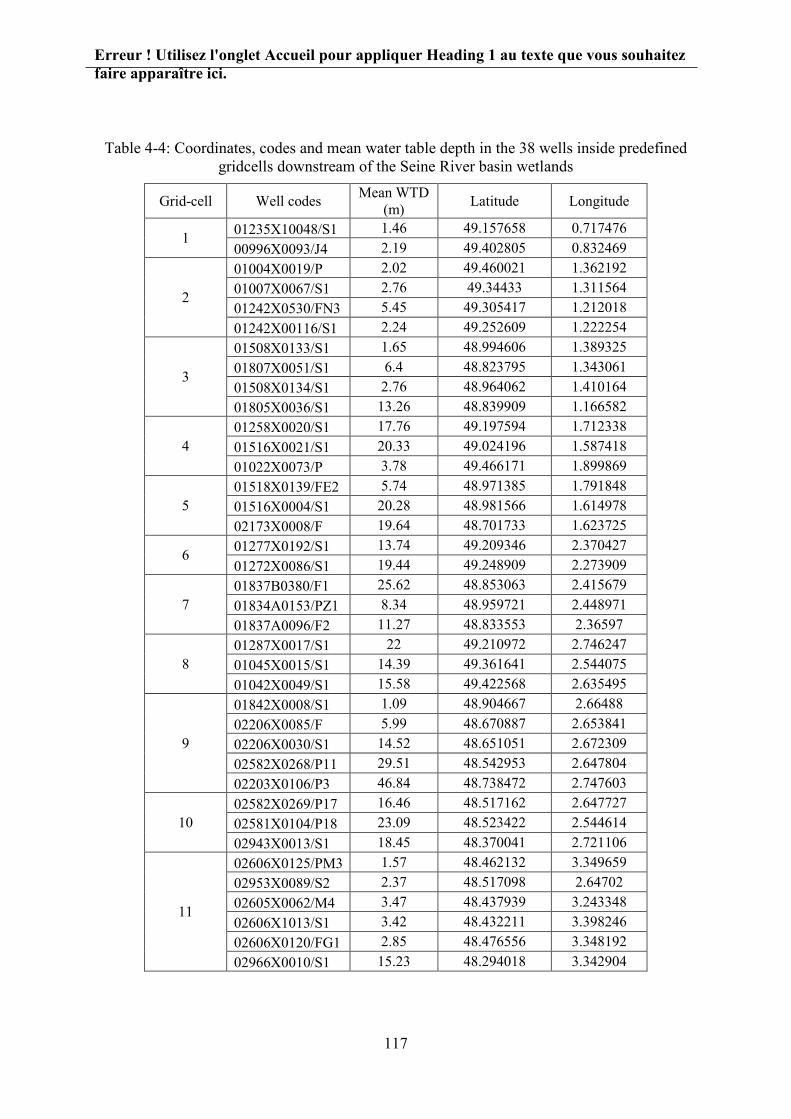
Erreur ! Utilisez l'onglet Accueil pour appliquer Heading 1 au texte que vous souhaitez faire apparaître ici.
117
Table 4-4: Coordinates, codes and mean water table depth in the 38 wells inside predefined gridcells downstream of the Seine River basin wetlands
Grid-cell Well codes Mean WTD (m) Latitude Longitude
1 01235X10048/S1 1.46 49.157658 0.717476 00996X0093/J4 2.19 49.402805 0.832469
2
01004X0019/P 2.02 49.460021 1.362192 01007X0067/S1 2.76 49.34433 1.311564 01242X0530/FN3 5.45 49.305417 1.212018 01242X00116/S1 2.24 49.252609 1.222254
3
01508X0133/S1 1.65 48.994606 1.389325 01807X0051/S1 6.4 48.823795 1.343061 01508X0134/S1 2.76 48.964062 1.410164 01805X0036/S1 13.26 48.839909 1.166582
4 01258X0020/S1 17.76 49.197594 1.712338 01516X0021/S1 20.33 49.024196 1.587418 01022X0073/P 3.78 49.466171 1.899869
5 01518X0139/FE2 5.74 48.971385 1.791848 01516X0004/S1 20.28 48.981566 1.614978 02173X0008/F 19.64 48.701733 1.623725
6 01277X0192/S1 13.74 49.209346 2.370427 01272X0086/S1 19.44 49.248909 2.273909
7 01837B0380/F1 25.62 48.853063 2.415679 01834A0153/PZ1 8.34 48.959721 2.448971 01837A0096/F2 11.27 48.833553 2.36597
8 01287X0017/S1 22 49.210972 2.746247 01045X0015/S1 14.39 49.361641 2.544075 01042X0049/S1 15.58 49.422568 2.635495
9
01842X0008/S1 1.09 48.904667 2.66488 02206X0085/F 5.99 48.670887 2.653841 02206X0030/S1 14.52 48.651051 2.672309 02582X0268/P11 29.51 48.542953 2.647804 02203X0106/P3 46.84 48.738472 2.747603
10 02582X0269/P17 16.46 48.517162 2.647727 02581X0104/P18 23.09 48.523422 2.544614 02943X0013/S1 18.45 48.370041 2.721106
11
02606X0125/PM3 1.57 48.462132 3.349659 02953X0089/S2 2.37 48.517098 2.64702 02605X0062/M4 3.47 48.437939 3.243348 02606X1013/S1 3.42 48.432211 3.398246 02606X0120/FG1 2.85 48.476556 3.348192 02966X0010/S1 15.23 48.294018 3.342904

Erreur ! Utilisez l'onglet Accueil pour appliquer Heading 1 au texte que vous souhaitez faire apparaître ici.
118
The fourth and last set of validation data is the anomaly of the terrestrial water storage
(TWS). TWS is the sum of all components of water in the hydrological system. In other words,
it is the sum of all the volume (runoff, river, subsurface) and water reservoirs like the water
stored in the unsaturated part of the soil column and the groundwater. This variable is
comparable to observations of total mass and gravity anomalies from space by satellite missions
like Gravity Recovery and Climate Experiment (GRACE). GRACE satellite was jointly
launched by NASA and the German Aerospace Center on March 2002 and finished its mission
on October 2017. GRACE satellite mission was the first remote sensing mission to provide
temporal variations of Terrestrial Water Storage (TWS). GRACE measures the mass variability
caused by a variety of geophysical processes like runoff and groundwater storage on land
masses, exchanges between ice sheets or glaciers with the ocean, and mass changes from
earthquakes (Frappart and Ramillien, 2018). In this study, we used the average of the three
solutions to GRACE measurements to smoothen the differences. These solutions used different
parameters and strategies such as different degree and order, spherical harmonic coefficient,
spatial filter and smoothing factor. The first one is that of the Center for Space Research (CSR)
which use GRACE level-1 observations without any additional smoothing or empirical de-
striping at 1 degree resolution (Save et al., 2016). The second one is the solution calculated at
Jet Propulsion Laboratory (JPL) which is originally represented on a 0.5 degree lon-lat grid,
aggregated to 1 degree (Watkins et al., 2015; Wiese et al., 2016). The third solution or that of
GeoForschungsZentrum (GFZ) again at 1 degree resolution (Dahle et al., 2014). The
comparisons are made for average values over the basin for GRACE and ORCHIDEE-WET.
Also, we assume that the land mass changes are solely due to water exchanges.
GRACE measurements are at coarse spatial resolutions (around 300 km), but are viable
sources for monitoring regional groundwater resources. Yet, since it requires external
information on surface water and snow packs, it contains uncertainty in measuring groundwater
storages. Alone or in combination with external datasets, the GRACE data provide a new source
of information on extreme climatic events, such as exceptional droughts and floods. Yet the
accuracy of GRACE is a few millimeters of Equivalent Water Height (EWH) over areas of
400 ×400 km (Wahr et al., 1998) and 0.7 cm EWH for a drainage area of 400,000 km2, and
0.3 cm for a drainage area of 4,000,000 km2 (Swenson et al., 2003).

Erreur ! Utilisez l'onglet Accueil pour appliquer Heading 1 au texte que vous souhaitez faire apparaître ici.
119
There are different approaches for estimating groundwater storage using the GRACE
data. The direct approach is removing the contributions of different hydrological reservoirs to
obtain the change in groundwater reservoir:
Δ𝑇𝑇𝑊𝑊𝑆𝑆 = Δ𝑊𝑊𝑠𝑠𝑉𝑉𝑤𝑤𝑜𝑜𝑝𝑝𝑝𝑝𝑉𝑉 + Δ𝑊𝑊𝑠𝑠𝑉𝑉𝑣𝑣𝑉𝑉 𝑉𝑉𝑉𝑉𝑣𝑣𝑠𝑠𝑇𝑇𝑉𝑉𝑤𝑤𝑉𝑉 + Δ𝑊𝑊𝑠𝑠𝑖𝑖𝑉𝑉𝑤𝑤 𝑝𝑝𝑝𝑝𝑝𝑝𝑝𝑝 + Δ𝑊𝑊𝜌𝜌𝑤𝑤𝑉𝑉𝑉𝑉𝑖𝑖𝑣𝑣𝑤𝑤𝑝𝑝𝑇𝑇𝑉𝑉𝑤𝑤
Δ𝑇𝑇𝑊𝑊𝑆𝑆 is measured by GRACE and by subtracting different components of terrestrial
water from it, Δ𝑊𝑊𝜌𝜌𝑤𝑤𝑉𝑉𝑉𝑉𝑖𝑖𝑣𝑣𝑤𝑤𝑝𝑝𝑇𝑇𝑉𝑉𝑤𝑤 can be estimated. In arid and semi-arid environments, where
surface water is negligible and snow pack inexistent, the equation is simplified to water
contained in soil. Examples of these regions are the High Plains aquifer in the United States,
Canning aquifer in Northwest Australia and the Middle East. But in more complex terrains
where surface water is not negligible, this reservoir should be extracted using insitu data, or
land surface model outputs like GLDAS (Global Land Data Assimilation System:
https://ldas.gsfc.nasa.gov/gldas/) in southeast Australia (Leblanc et al., 2009).
4.4 Simulation results and comparisons to observations with ORCHIDEE-
REF
After configuring the model for the simulations, we performed several tests on the
ORCHIDEE to assure that the parameters (like the reservoir property and the exchange factor)
are within a reasonable range when compared to observations of river flow, evapotranspiration
and groundwater. Some of these tests are done using the ORCHIDEE-REF, notably those aimed
at selecting one of the set of forcing files and testing the reservoir time constants (reservoir
property). The other simulations are done using the ORCHIDEE-WET on the sensitivity to the
parameters (like exchange factor and the soil column depth) and also comparison to
groundwater observations.
4.4.1 Test runs on climate forcing
To determine the best set of atmospheric forcings for simulations, we first performed
test runs over the whole available period of each set of forcing files, with the ORCHIDEE-REF.
Then, the results were compared for the mutual period of all three forcings (1978-2011). The
results of this 34-year simulations with controlled model settings over the Seine River basin
were used to evaluate certain model outputs with observed values. The results of the first three
years of simulation are excluded to let the model initiate the variables and avoid the effect of

Erreur ! Utilisez l'onglet Accueil pour appliquer Heading 1 au texte que vous souhaitez faire apparaître ici.
120
initial conditions. These evaluations are presented for river discharge at the basin outlet (the
most downstream hydrometric station, Poses) and the mean evapotranspiration over the basin.
For the river discharge, the seasonality of the simulated flow is reasonably similar to
observed values. Yet, CRU-NCEP forcing results in lower flow values (28% smaller than
observation), while WFDEI and GSWP3 show higher flow values (27 and 0% larger
respectively as shown in Table 4-5). The base-flows are better simulated with CRU-NCEP
forcing but seasonality is also more pronounced with this forcing (Figure 4-13a).
Figure 4-13: Monthly means of simulated values with different forcings and reference ORCHIDEE of (a) river discharge (m3.s-1) at Poses station against observation, (b)
Evapotranspiration rate (mm/day) against observed values (Jung et al., 2010), (c) Soil moisture (kg/m2), and (d) Bare soil evaporation (mm/day), during the period 1981-2005
Generally, considering all the statistical indices, it appears that CRU-NCEP forcing
leads to better simulated river discharge values compared to observations at Poses. However,
Jan Feb Mar Apr May Jun Nov DecJul Aug Sep Oct
Mean543389760688
Jan Feb Mar Apr May Jun Nov DecJul Aug Sep Oct
mm
/day
mean1.471.511.281.41
Jan Feb Mar Apr May Jun Nov DecJul Aug Sep Oct
Kg/m
2
Jan Feb Mar Apr May Jun Nov DecJul Aug Sep Oct
mm
/day
(a) (b)
(c) (d)552
594592
Mean0.41
Mean
0.330.41
Disc
harg
e (m
3 /s)
ET
Soil
moi
stur
e
Bare
soil
evap
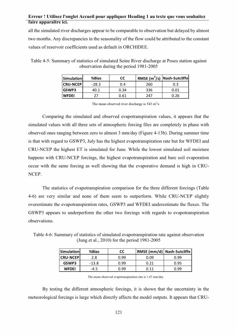
Erreur ! Utilisez l'onglet Accueil pour appliquer Heading 1 au texte que vous souhaitez faire apparaître ici.
121
all the simulated river discharges appear to be comparable to observation but delayed by almost
two months. Any discrepancies in the seasonality of the flow could be attributed to the constant
values of reservoir coefficients used as default in ORCHIDEE.
Table 4-5: Summary of statistics of simulated Seine River discharge at Poses station against observation during the period 1981-2005
The mean observed river discharge is 543 m3/s
Comparing the simulated and observed evapotranspiration values, it appears that the
simulated values with all three sets of atmospheric forcing files are completely in phase with
observed ones ranging between zero to almost 3 mm/day (Figure 4-13b). During summer time
is that with regard to GSWP3, July has the highest evapotranspiration rate but for WFDEI and
CRU-NCEP the highest ET is simulated for June. While the lowest simulated soil moisture
happens with CRU-NCEP forcings, the highest evapotranspiration and bare soil evaporation
occur with the same forcing as well showing that the evaporative demand is high in CRU-
NCEP.
The statistics of evapotranspiration comparison for the three different forcings (Table
4-6) are very similar and none of them seem to outperform. While CRU-NCEP slightly
overestimate the evapotranspiration rates, GSWP3 and WFDEI underestimate the fluxes. The
GSWP3 appears to underperform the other two forcings with regards to evapotranspiration
observations.
Table 4-6: Summary of statistics of simulated evapotranspiration rate against observation (Jung et al., 2010) for the period 1981-2005
The mean observed evapotranspiration rate is 1.47 mm/day
By testing the different atmospheric forcings, it is shown that the uncertainty in the
meteorological forcings is large which directly affects the model outputs. It appears that CRU-
Simulation %Bias CC RMSE (m3/s) Nash-SutcliffeCRU-NCEP -28.3 0.4 260 0.3GSWP3 40.1 0.34 336 0.01WFDEI 27 0.61 247 0.26
Simulation %Bias CC RMSE (mm/d) Nash-SutcliffeCRU-NCEP 2.8 0.99 0.09 0.99
GSWP3 -13.8 0.99 0.21 0.95WFDEI -4.5 0.99 0.11 0.99
Erreur ! Utilisez l'onglet Accueil pour appliquer Heading 1 au texte que vous souhaitez faire apparaître ici.
122
NCEP and WFDEI forcings performs better with ORCHIDEE-REF for the Seine River basin
simulations with regard to observations. Here it is decided to choose the CRU-NCEP
meteorological forcing for the following since it has longer data period than WFDEI. Therefore,
for further steps with simulation on ORCHIDEE-REF and ORCHIDEE-WET, we will focus
on CRU-NCEP forcing.
4.4.2 Tests on the different routing time constants
The ORCHIDEE-REF outputs appear to be very sensitive to changes in the values of
the time constants of the reservoirs. To modify the time constants of the reservoirs, several
values of reservoir properties are tested in simulations. In this section and the following, what
is called the Reference simulation is the one performed with ORCHIDEE-REF for default
values of time constants and with CRU-NCEP atmospheric forcings (the details of parameters
for this simulation are explained in Table 4-3).
In this step, the simulations are performed for the period 1960-2014. Again, to let the
variables spin up and reach a constant level, we exclude the first three years of the simulation
in the analysis. As expected, by decreasing the time constants, the simulated flow is advanced
in time and more seasonally variant (Figure 4-14). By increasing the seasonality with the
decreased time constants, the base flow drops down to near 50 m3.s-1 as compared to almost
200 m3.s-1 in the Poses station. But the peak of the annual flow is correctly in February for all
three simulations with decreased time constants, where in the reference simulation the peak
flow is delayed for almost two months. The results of the simulations are very similar for
TCST/5 and TCST/10. It appears that decreasing the time constant more than five times will
not change the shape of the hydrograph. As we decrease the time constants, the resulting flow
is less affected by the routing scheme. This means that the hydrograph without the routing is
very close to the hydrographs with TCST/10. Another simulation is also performed with
increased slow reservoir time-constant to test the sensitivity of surface variables with respect to
reservoir property (TCST-Slow×3). In this simulation, we multiplied the slow reservoir time-
constant by three and left the other time-constants as their default values. Increasing the time-
constant results in a smoother river flow with decreased amplitude of the variations. The river
flow, in this simulation, varies between 305 to 484 m3/s. This decreased variance of the river
flow shows the important role of the time-constants of the slow reservoir in shaping the
hydrograph.

Erreur ! Utilisez l'onglet Accueil pour appliquer Heading 1 au texte que vous souhaitez faire apparaître ici.
123
Figure 4-14: Monthly mean of Seine River simulated discharges at Poses station with different values of time constants compared to reference simulation and observed values for
the period 1963-2014
The simulated flow appears to be more in phase with the observation when the time
constant is decreased (Table 4-7). This is particularly true for the wet season, while the
simulated flows of the dry seasons are moderately underestimating the base flow. This means
that the flows are faster in the Seine River basin in comparison to the Senegal basin for which
ORCHIDEE has been calibrated. But since performing a comprehensive calibration of
ORCHIDEE for the Seine River basin is out of the scope of this study, for the incoming sections
we will use the default ORCHIDEE time constants (those in the reference simulation).
Table 4-7: Summary of statistics of simulated Seine River discharge at Poses station with different time constants against observation 1963-2014
The mean observed river discharge is 545 m3/s
Since the different values of time-constants do not change distribution of water inside
the soil column, there is no effect of changing time-constants on the evapotranspiration rates
Rive
r dis
char
ge m
3 /s
Jan Feb Mar Apr May Jun Nov DecJul Aug Sep Oct
Mean (m3/s)
543389339340340387
Simulation %Bias CC RMSE (m3/s) Nash-SutcliffeReference -28.3 0.4 267 0.33TCST/2 -37.5 0.97 214 0.64TCST/5 -37.3 0.98 207 0.65TCST/10 -37.3 0.98 206 0.64TCST-Slowx3 -28.7 0.1 277 -0.5

Erreur ! Utilisez l'onglet Accueil pour appliquer Heading 1 au texte que vous souhaitez faire apparaître ici.
124
and other surface variables; the only change is observed for the river flow due to changes in the
reservoir volumes (Figure 4-15). As shown in this figure the stream reservoir is almost empty
during the year for the simulation with tripled slow reservoir time constant, leading to increased
river flow compared to other simulations.
Figure 4-15: Monthly mean of Seine River simulated (a) stream reservoir volume (kg/m2) and (b) fast reservoir volume (kg/m2) for the period 1963-2014
4.4.3 Contribution of the different flow components
In ORCHIDEE, without the wetland element, the components of the flow can have
different contributions to the total flow. In the Seine River basin, the contribution of the
groundwater (controlled by the slow reservoir coefficient) is more than 90% of the total flow
(Figure 4-16). In Figure 4-16, the yellow line is the drainage or the groundwater flow while the
red line is the surface runoff component of the flow. The blue line is the total river flow if no
routing is considered and the grey line is the delayed flow with routing. Two main points are
derived from this figure. The first one is the dominant role of the drainage in the final river flow
and consequently the strong sensitivity of the flow to slow reservoir time constant. Second is
the observation that the total flow without routing is more similar to observed river discharge
than that with the routing. This latter means that the default reservoir time constants
(particularly that of slow reservoir) are high and lead to delayed flow.
Stre
am re
serv
oir v
olum
e (k
g/m
2 )
Jan Feb Mar Apr May Jun Nov DecJul Aug Sep OctMonths
Fast
rese
rvoi
r vol
ume
(kg/
m2 )
Jan Feb Mar Apr May Jun Nov DecJul Aug Sep OctMonths
(a) (b)

Erreur ! Utilisez l'onglet Accueil pour appliquer Heading 1 au texte que vous souhaitez faire apparaître ici.
125
Figure 4-16: Monthly mean values of different simulated components of the flow for the ORCHIDEE-REF simulation with CRU-NCEP forcing over the Seine River basin at Poses
station against observation for the period 1963-2014 (the values of drainage and surface runoff are transformed from mm/day to m3/s by multiplying to Seine River basin area)
4.5 Comparison between ORCHIDEE-REF and ORCHIDEE-WET
The previous section aimed at analyzing the ORCHIDEE-REF version and its sensitivity
to meteorological forcings and reservoir time constants. In this section, the objective is to assess
the changes in river discharge when the wetland scheme is added to ORCHIDEE.
4.5.1 Comparison of ORC-REF and ORC-WET with different forcings
At this step, it is necessary to decide on the forcing sets to continue testing the model
parameters. Earlier, using the ORCHIDEE-REF, we evaluated CRU-NCEP to be the best
forcing. Here, we do an additional test on ORCHIDEE-WET with different forcings to evaluate
their performance with the wetland component. In this test, the depth of soil column is assumed
to be two meters, the exchange factor between the wetland soil-tile and the stream is set to 1000,
and the wetland fractions for each grid-cell is read from the CW-WTD map.
Rive
r dis
char
ge m
3 /s
Feb Apr June Aug Oct DecMonths

Erreur ! Utilisez l'onglet Accueil pour appliquer Heading 1 au texte que vous souhaitez faire apparaître ici.
126
Figure 4-17: Monthly mean values of river discharge for ORCHIDEE-REF and ORCHIDEE-WET simulations over the Seine River basin at Poses station against observation for the
period 1963-2014
The CRU-NCEP (GW) and WFDEI (GW) simulations are seemingly closer to
observations with advanced peak flows towards the winter time. Although applying the GW
components leads to decreased annual flow, the decrease for CRU-NCEP leads to larger
absolute bias while it is the opposite for WFDEI and GSWP. The statistical model efficiency
factors like correlation coefficient also shows that CRU-NCEP and WFDEI are both closer to
observations compared to GSWP3 forcing set, and the river discharges with WFDEI and CRU-
NCEP forcings are overestimated.
Table 4-8: Summary of statistics of simulated Seine River discharge at Poses station with
different forcing sets and versions against observation 1963-2014
The mean observed river discharge is 542 m3/s
Mean
542389338760725688653
Jan Feb Mar Apr May Jun Nov DecJul Aug Sep Oct
Rive
r Dis
char
ge m
3 /s
Months
(WET)
(WET)
(WET)
Forcing %Bias CC RMSE (m3/s) Nash-SutcliffeCRU-NCEP (REF) -28.3 0.4 260 0.3CRU-NCEP (WET) -37.6 0.98 218 0.42GSWP (REF) 40.1 0.34 336 0.01GSWP (GW) 33.6 0.97 191 0.07WFDEI (REF) 27 0.61 247 0.26WFDEI (GW) 20.3 0.98 124 0.33

Erreur ! Utilisez l'onglet Accueil pour appliquer Heading 1 au texte que vous souhaitez faire apparaître ici.
127
For all the forcings, including the wetland component leads to better river discharges
compared to observation. Also, the simulated values of the river discharge among all for
forcings the CRU-NCEP and WFDEI compare better to observed river flow measurements at
Poses station and reanalysis of Jung et al., (2010). For all forcings, the wetland scheme causes
an increase between 3 to 6% in the evapotranspiration rates, but no major enhancement with
regard to observations is detected (not shown).
WFDEI and CRU-NCEP show almost equal similarity to observation both for reference and
GW simulation (while sometimes WFDEI is more similar). At this step one set of forcing files
should be selected for the future simulations. Therefore, since the data period for WFDEI starts
in 1978 we select CRU-NCEP as the best forcing set. After deciding on the choice of the
atmospheric forcings, and the relevant time constants for different reservoirs (default values)
we focus our simulations on the ORCHIDEE-WET version. In this section and the following,
what is called the Reference simulation is the one performed with ORCHIDEE-REF for default
values of time constants and with CRU-NCEP atmospheric forcings (Table 4-3).
4.5.2 Test runs to compare surface variables with and without the existing GW
parametrization
The routing scheme of ORCHIDEE-REF delays the simulated river discharge at Poses,
and attenuates the seasonal contrasts between high and low flow, compared to total runoff. Most
of this effect is due to the slow reservoir of the routing scheme, which is designed to represent
the groundwater flow, owing to a longer residence time (TCST) than the other two reservoirs.
To demonstrate this, we tested a simulation (REF-noGW) where the residence time of this
groundwater reservoir is given the same value as the one of the stream reservoir, so that the
buffering effect by groundwater flow is absent (Figure 4-18).

Erreur ! Utilisez l'onglet Accueil pour appliquer Heading 1 au texte que vous souhaitez faire apparaître ici.
128
Figure 4-18: Monthly means of simulated values of river discharge (m3.s-1) at Poses station for reference ORCHIDEE, ORCHIDEE without the GW parametrization and ORCHIDEE-
WET against observation 1963-2014
Figure 4-18 confirms that this simulation REF-noGW (the green line) is advanced in
comparison to ORCHIDEE-REF, but also shows that ORCHIDEE-WET is further advanced,
and best matches observed flows. The reason for early peak flows in ORCHIDEE-WET is that
inflow from the upland fraction makes the lowland fraction more humid (as shown in Figure
4-19), especially in winter, so that this fraction quickly produces surface runoff when it rains.
The low flows are also better phased (earlier than in REF), because of increased
evapotranspiration in ORCHIDEE-WET during the summer time. This increased
evapotranspiration, however, enhances the overestimation of simulated evapotranspiration
found with the CRU-NCEP forcing, but it might correct the underestimation of
evapotranspiration found with ORCHIDEE-REF and the other two forcing (mean
evapotranspiration of 1.41 and 1.27 mm/d with WFDEI and GSWP3 respectively, compared to
1.47 mm/d based on Jung et al., 2010).
Rive
r dis
char
ge m
3 /s
Jan Feb Mar Apr May Jun Nov DecJul Aug Sep Oct
Mean (m3/s)
389402339
542
Months
-WET-noGW

Erreur ! Utilisez l'onglet Accueil pour appliquer Heading 1 au texte que vous souhaitez faire apparaître ici.
129
Figure 4-19: The mean water content profile for upland and lowland in the ORCHIDEE-WET simulation (with CRU-NCEP forcing), on average over the Seine River basin and the period
1963-2014
4.6 Sensitivity tests on ORCHIDEE-WET
CW-WTD map is aggregated to the 0.5° resolution and used to attribute values of
lowland fractions (fraction of the fourth soil tile) to grid-cells. First, we assured that the water
balance is held. Then, we tested the model for sensitivity of the wetland parameters and
parameters of their hydrology. These sensitivity tests are performed in order to understand the
behavior of the new wetland scheme in ORCHIDEE-WET. Several tests are performed in this
section: on sensitivity of the exchange factor between the wetland soil column and the river, on
the impact of different constant wetland fractions, and on the different depths of the soil column.
4.6.1 Sensitivity to Exchange Factor
Test runs with different exchange factors were performed in order to find the reasonable
range of this factor for further simulations. In the following, comparisons for some of the
variables are shown with respect to different exchange factors. It should be reminded that in an
isotropic idealized aquifer, the a priori value of the exchange factor is estimated as 𝜋𝜋2
4~2.5 as
discussed in chapter 2. But here, three values of exchange factor between 100 and 10000 are
tested. This wide range is chosen considering the effect of higher conductivities in the
Water content (m3/m3)
WTD
(m)
satu
ratio
n

Erreur ! Utilisez l'onglet Accueil pour appliquer Heading 1 au texte que vous souhaitez faire apparaître ici.
130
horizontal direction and the overestimation of B (the lowland width) since it is calculated based
on the drainage density of the whole grid and not only the lowland fraction.
Comparing the monthly mean river discharges for different values of the Exchange
Factor (EF) shows that by increasing the EF the base flow (river discharge in the dry period
from July to September) increases and generally the dry-period flow is delayed (Figure 4-20a).
When EF is increased, the water in the water table is evacuating the soil column with a higher
rate. We have higher flows for EF=10000 during February to mid-September, because
evapotranspiration decreases due to a lower soil moisture and a deeper water table. On the other
hand, by deepening the water table, the flow is lower in simulations with high EF for the winter
period.
Figure 4-20: Monthly means of simulated values with different exchange factors and ORCHIDEE-WET of (a) river discharge (m3.s-1) at Poses station against observation 1963-
2014, (b) Evapotranspiration rate (mm/day) against Observed values (Jung et al., 2010) 1980-2014, (c) Soil moisture (kg/m2), (d) Water table depth (m), and (e) the base flow (mm/day)
during the period for the period 1963-2014
Jan Feb Mar Apr May Jun Nov DecJul Aug Sep Oct
Rive
r disc
harg
e m
3 /s
Mean (m3/s)
542389335338357
0.0
0.5
1.0
1.5
2.0
Jan Feb Mar Apr May Jun Nov DecJul Aug Sep Oct
Jan Feb Mar Apr May Jun Nov DecJul Aug Sep Oct
mean552620616598
Jan Feb Mar Apr May Jun Nov DecJul Aug Sep Oct
mean
1.51
1.55
1.47
1.571.58(a)
(b)
(c)(d)
Soil
moi
stur
e (k
g/m
2 )
Evap
otra
nspi
ratio
n (m
m/d
ay)
Wat
er ta
ble
dept
h (m
)
Jan Feb Mar Apr May Jun Nov DecJul Aug Sep Oct
(e)
0.29Mean
0.380.77
0.017Mean
0.1340.336
Base
flow
(mm
/day
)

Erreur ! Utilisez l'onglet Accueil pour appliquer Heading 1 au texte que vous souhaitez faire apparaître ici.
131
The reference simulation (ORCHIDEE-REF) does not capture the seasonal dynamic of
the river discharge and shows delayed flow rates all year long. Statistical evaluation criteria
show that the similarity between monthly mean values is higher for EF=1000. The correlation
coefficient between simulations and observed values soars from 0.4 in ORCHIDEE-REF to
0.98 for EF=1000. The same increase in the Nash-Sutcliffe index is observed (Table 4-9). With
increased EF, the bias of the river discharge with regard to observation drops down to 25% in
the simulation with EF=1000, but the absolute bias decreases when it is increased. The
evapotranspiration rate (which is increased by introducing the ORCHDIEE-GW) slightly
decreases with the increasing EF (Figure 4-20b), presumably because of the water table
deepening particularly during the summer and autumn. Also, since water leaves the wetland
soil column in a higher rate with high EF, the overall soil moisture moderately decreases.
Table 4-9: Summary of statistical similarity indices for the river discharge in simulations of exchange factor sensitivity compared to observations at Poses station for the period 1963-
2014
The mean observed river discharge is 542 m3/s
The partition of transpiration to total evapotranspiration is almost 65% and most of the
decrease in total evapotranspiration by increasing EF is due to plant transpiration.
As observed in Figure 4-21, the values of river flow and evapotranspiration rate are
rather stable for exchange factors ranging from 100 to 1000 but change rapidly for values larger
than 1000. After testing the sensitivity of the ORCHIDEE-WET based on different values of
the exchange factor, we decided to use EF=1000 for the following. Since the surface variables
are interconnected with each other, the exchange factor cannot be independently calibrated with
varying wetland fractions and soil depths and also atmospheric forcings.
Simulation %Bias CC RMSE (m3/s) Nash-SutcliffeReference -28.3 0.4 260 0.3EF=100 -38.2 0.97 221 0.34EF=1000 -37.6 0.98 218 0.42EF=10000 -34.3 0.94 210 0.43

Erreur ! Utilisez l'onglet Accueil pour appliquer Heading 1 au texte que vous souhaitez faire apparaître ici.
132
Figure 4-21: Mean values of Simulated (a) river discharge at the Poses station, (b) evapotranspiration rate over the Seine River basin, (c) mean water table depths and (d) the
baseflow for three different values of exchange factor over the period 1963-2014 (the x-axis is logarithmic)
4.6.2 Sensitivity to the wetland fractions
In previous tests, we used the CW-WTD wetland map to prescribe the wetland fractions
over the Seine River basin. The wetland fraction at 0.5° resolution in this map differs from 0 to
0.73 in different parts of the Seine River basin. In order to test the model performance for cases
with high and low wetland fractions, we scheduled some tests with constant 0.05, 0.1, 0.25, 0.5
and 0.75 wetland fractions. All these tests were done using the constant EF=1000. Results of
these tests show that higher wetland fraction increases the seasonality of the river discharge and
causes mean decrease of flow and in particular during the dry months (Figure 4-22a). Yet, the
sensitivity of the flow to wet fractions is maximum for small wet fractions and becomes almost
zero for wet fraction > 0.5 of the pixel. The direction of the change in volume of flow is different
during the winter season. During January to March, when water availability is high, soil is
almost saturated all the time and all the entering water from the upland drainage during the dry
period (used to fill up the wetland soil column) is directly discharged to rivers. The increase of
the river discharge with higher wetland fraction during the winter time is the result of a
complicated process. With high wetland fractions, although the drainage from upland decreases
but since the drainage in the wetland is blocked, precipitation is directly drained to the stream,
0.41
0.415
0.42
0.425
0.43
0.435
0.44
0.445
10 100 1000 10000 100000
Ri
ver d
isch
arge
mm
/day
1.55
1.555
1.56
1.565
1.57
1.575
10 100 1000 10000 100000
Evap
otra
nspi
ratio
n m
m/d
ay
Exchange factor
0
0.1
0.2
0.3
0.4
0.5
0.6
0.7
0.8
0.9
10 100 1000 10000 100000
Wat
er ta
ble
dept
h (m
)
Exchange factor
0
0.05
0.1
0.15
0.2
0.25
0.3
0.35
0.4
10 100 1000 10000 100000
Base
-flow
(mm
/day
)
(a)
(b)
(c)
(d)

Erreur ! Utilisez l'onglet Accueil pour appliquer Heading 1 au texte que vous souhaitez faire apparaître ici.
133
increasing the total river discharge. Also, there appears to be a shift in wet season high flow
with increased constant wetland fraction. Although the low flow season appears to have
remained between July to October for different simulations, the wet season peak month is
gradually shifted from March for simulation with 0.05 wetland fraction, to February for
simulation with wetland fractions higher than 0.1. This comparison contradicts the traditional
role of wetlands in decreasing the seasonality; adding the wetland component in ORCHIDEE-
WET generally increases the discharge seasonality. Generally, the residence time of the water
is shorter with larger wetland fraction. When the potential wetland extent is high, large wetlands
may appear with short retention times that increases the seasonality.
Figure 4-22: Monthly means of simulated values with different wetland fractions and ORCHIDEE-WET of (a) river discharge (m3.s-1) at Poses station against observation 1963-
2014, (b) Evapotranspiration rate (mm/day) against Observed values (Jung et al., 2010) 1980-2014, (c) Soil moisture (kg/m2) and (d) Bare soil evaporation (mm/day), during the period for
the period 1963-2014
A part of the increase in river flow seasonality over the Seine River basin is caused by
the increase in evapotranspiration with respect to the increase in wetland fraction (Figure
4-22b). More wetland fraction translates into more evaporative surface with near potential rate.
This rate is maximum during the summer period when often the water supply is limited,
therefore when there are more wetlands there is more evapotranspiration during summer which
Jan Feb Mar Apr May Jun Nov DecJul Aug Sep Oct
Mean0.400.410.410.420.430.44
Jan Feb Mar Apr May Jun Nov DecJul Aug Sep Oct
Mean552566580615657686
Jan Feb Mar Apr May Jun Nov DecJul Aug Sep Oct
Evap
otra
nspi
ratio
n (m
m/d
ay)
Mean (mm/day)
1.471.511.531.541.581.601.62
Jan Feb Mar Apr May Jun Nov DecJul Aug Sep Oct
Rive
r dis
char
ge m
3 /s
Mean542389376365338311297
(a) (b)
(d)(c)
Soil
moi
stur
e (k
g/m
2 )
Bare
soil
evap
orat
ion
(mm
/day
)

Erreur ! Utilisez l'onglet Accueil pour appliquer Heading 1 au texte que vous souhaitez faire apparaître ici.
134
ends in decreased flow. This also means that groundwater from the upland is sustaining the
evapotranspiration at almost potential rates even when precipitation is far less than the
atmospheric demand. In all cases, simulated ET is 7 to 14% higher than observed values.
The evapotranspiration over the Seine River basin is increased in simulations as the
wetland fraction becomes more important. But this increase is not linear. In other words, we do
not see two times more evapotranspiration when changing the wet fraction from 0.25 to 0.5.
Figure 4-23: Monthly means simulated water table depth over the Seine River basin for different values of constant wet fraction for the period 1963-2014
The summer time increase in evapotranspiration compared to varying wetland fractions
is mostly induced by the increase in plant transpiration in summer and early autumn, but also
by the bare soil evaporation (Figure 4-22c). The patterns of increase in bare soil evaporation
with different wetland fractions are very similar to that of total evapotranspiration within the
second half of the year. During the winter and autumn, there is no change in evapotranspiration
since it is the evaporative demand that has the controlling role, and not the water supply. But
during the spring and summer, the evaporation from bare surface increases as there is more
water to evaporate in the prescribed wetland fractions.
Bare soil evaporation is almost completely identical during the wet season
independently from wetland fractions. Higher bare soil evaporation is simulated with higher
wetland fractions because there is more surface with direct interaction with atmosphere (Figure
4-22c). Bare soil evaporation rate is a function of atmospheric evaporative demand and the soil
0.0
0.5
1.0
1.5
2.0
Wat
er ta
ble
dept
h (m
eter
s)
Jan Feb Mar Apr May Jun Nov DecJul Aug Sep Oct
mean
0.060.150.400.690.81

Erreur ! Utilisez l'onglet Accueil pour appliquer Heading 1 au texte que vous souhaitez faire apparaître ici.
135
moisture. Therefore, although the demand is high during the summer, the evaporation rates are
not at the annual maximum. Another interesting point is that the increase in bare soil
evaporation is not in linear relationship with wetland fraction. In other words, when the wetland
fraction is increased, the water table drops down and the connection between the groundwater
and the atmosphere becomes weaker. Therefore, the increased bare soil evaporation is
maximum for small fraction of wetland.
The soil moisture responds to changes in the wetland fraction over the basin as well
(Figure 4-22d). It goes up with increased wetland fraction. This is in line with the increased
evapotranspiration. The seasonality of the soil moisture is almost two months delayed with
respect to evapotranspiration rates. The increase in soil moisture with varying wetland fractions
is almost constant for all the months and appears to be in linear relationship with the wetland
fraction. For a soil column depth of two meters, one percent increase in wetland fraction leads
to about 1.4 kg.m-2 increase in soil moisture.
When the wetland fraction is very small (<0.1), the water table stands very close to
surface as for the case with 5% of wetland fraction in Figure 4-23. When the wetland fraction
is increased there is more space in the wetland soil tile for water table to build up and hence the
water table drops down. The other reason for this drop down is the decreased incoming water
from the drainage in upland.
In Chapter 3, when describing wetlands we defined them as regions with a water table
shallower than 20 cm. However, when the potential wetland fraction is increased in
ORCHIDEE-WET (for wetland fraction higher than 0.25), the water table is shown to be deeper
than 20 cm, all year. With the water table depth within the soil-tile, we have increased
evapotranspiration which is a sign of wet soils. This means that even when the water table is
deeper than the water table threshold, in some zones, properties and effects of wetlands are
witnessed.
4.6.3 Sensitivity to the soil column depths
As said before, the default soil column depth in ORCHIDEE and ORCHIDEE-WET is
two meters. However, in order to inspect the effect of soil depth on surface variables we
performed several tests with soil depths ranging from 2 m to 20 m. In these tests the wetland
fraction is set to the CW-WTD map. In the ORCHIDEE-WET, the soil depth is similar for

Erreur ! Utilisez l'onglet Accueil pour appliquer Heading 1 au texte que vous souhaitez faire apparaître ici.
136
uplands and lowlands. Therefore, a mixed effect of the soil depth on surface variables is
observed. In order to adapt these soil depths to ORCHIDEE, the number of soil layers in the
hydrological scheme should be increased to 35, 50, 90 and 170 layers for 3, 5, 10 and 20 m soil
column depths respectively. At the first step, in order to make sure that the model and the soil
moisture is at equilibrium during the simulation period, the time-series of the soil moisture and
drainage from the upland is checked (Figure 4-24a,b). The soil column reaches an equilibrium
of soil moisture and drainage after one year. The multi-annual variation of the soil moisture and
drainage, however, becomes more important with the increasing soil depth.
Figure 4-24: Time-series of simulated (a) soil moisture and (b) drainage for different depths of the soil column, over the Seine River basin, for the period 1960-2014
The first analysis is made on the upland drainage values which show that increasing the
soil depth leads to a flattening of the seasonality (Figure 4-25). With deep soil columns, there
1960 20151970 1980 1990 2000 2010
1960 20151970 1980 1990 2000 2010
(a)
(b)
Soil
moi
stur
e (k
g/m
2 )Dr
aina
ge (m
m/d
ay)
Mean (kg/m2)616953161232186463
Mean (mm/day)0.380.290.290.280.280.29

Erreur ! Utilisez l'onglet Accueil pour appliquer Heading 1 au texte que vous souhaitez faire apparaître ici.
137
is a considerable volume for water accumulation in the upland soil column, so the precipitation
water infiltrates and is distributed in the upland soil column. This leads to decreased seasonality
of the drainage from the bottom of the upland soil column (Figure 4-25a). In other words, deep
soil column acts as a buffer for infiltrated water, which becomes smoother and delayed.
Consequently, the entering flux from the upland to wetland soil column is almost constant
during the year. The seasonality of the drainage is very sensitive to the soil column depth as
seen in the figure for the deepening of the soil column from two meters to three meters. The
monthly-mean values become constant when the soil column depth reaches about 10 meters
and stays constant for depths more than that.
Figure 4-25: Monthly means of simulated values with different soil column depths and ORCHIDEE-WET of (a) drainage rates (b) river discharge (m3.s-1) at Poses station against
observation, (c) Soil moisture (kg/m2), (d) water table depth anomaly (m), (e) the mean surface runoff (mm/day) and (f) evapotranspiration over the Seine River basin, during the
period 1963-2014
Jan Feb Mar Apr May Jun Nov DecJul Aug Sep Oct
Jan Feb Mar Apr May Jun Nov DecJul Aug Sep Oct
Surfa
ce ru
noff
(mm
/day
)
Mean (mm/day)
0.065
0.0650.0650.0650.0650.065
0.065
Jan Feb Mar Apr May Jun Nov DecJul Aug Sep Oct
mm
/day
Mean
0.290.290.280.280.29
0.38
Jan Feb Mar Apr May Jun Nov DecJul Aug Sep Oct
m3 /s
mean
338342357373389
422389
Jan Feb Mar Apr May Jun Nov DecJul Aug Sep Oct
kg/m
2
(a) (b)
(c) (d)
(e)
Jan Feb Mar Apr May Jun Nov DecJul Aug Sep Oct
Evap
otra
nspi
ratio
n (m
m/d
ay)
Mean (mm/day)
1.47
1.571.571.561.551.54
1.52
Soil
moi
stur
e (k
g/m
2 )
WTD
ano
mal
y (m
)
Drai
nage
(mm
/day
)
Rive
r disc
harg
e (m
3 /s)
(f)

Erreur ! Utilisez l'onglet Accueil pour appliquer Heading 1 au texte que vous souhaitez faire apparaître ici.
138
Most of the water flux to the wetland soil column comes from the upland drainage. As
a result, the seasonality of the river flow is also very sensitive to varying soil depths. River flow
at the Poses station is also nearly constant for cases with soil depths deeper than 10 meters
(Figure 4-25b). Another point is that, naturally, when the soil depth increases, the amount of
soil moisture in the soil column increases as well and this increase appears to be linear with the
soil depth (Figure 4-25c). However, the increase in soil moisture is not enough for the water
table to approach the surface for soil depths more than 3 meters. Therefore, the water table
depth is never shallower than 20 cm for soil column depths deeper than 3 meters (Figure 4-25d).
By increasing the soil column depth, the upland and lowland profiles for the first meters
of the soil become similar, particularly because of the insufficiency of soil moisture in providing
enough water to saturate the soil column. The upland soil column water content profile remains
almost the same for different soil columns depths with the maximum water content reaching
almost 0.3 at the bottom. There appears to be two main high sharp gradients in the lowland
(wetland) water content profile: one within the first one meter of the soil from the surface and
second within the deepest two meters. The atmospheric evaporative demand at the surface
causes the first gradient and the second one is caused by the injected water from the upland at
the bottom.

Erreur ! Utilisez l'onglet Accueil pour appliquer Heading 1 au texte que vous souhaitez faire apparaître ici.
139
Figure 4-26: The water content profile for upland and lowland, for different soil column depths, averaged over the Seine River basin, for the period 1963-2014, for the ORCHIDEE-
WET simulation with CRU-NCEP forcing
The water table depth appears to be very dependent on the wetland fraction in different
parts of the basin (Figure 4-27). Since in the Seine River basin, wetland fraction is higher in the
downstream (western parts of the basin), the water table is simulated to be deeper in those areas
(Figure 4-28). On the other hand, the water table depth is shallower in the upland basin, i.e
where the wetland fraction is low.
Figure 4-27: The wetland fraction at (a) 3 arc-min, and (b) 0.5° resolutions at the Seine River basin with regards to CW-WTD
0
2
4
6
8
10
0.2 0.25 0.3 0.35 0.4 0.45
0.2 0.25 0.3 0.35 0.4 0.45
0
1
2
3
4
5
0.2 0.25 0.3 0.35 0.4 0.45
0
5
10
15
20
WTD
(m)
Water content (m3/m3)
Water content (m3/m3)
Water content (m3/m3)
satu
ratio
n
satu
ratio
n
satu
ratio
n
WTD
(m)
WTD
(m)
0.0
0.1
0.2
0.4
0.6
0.8
1.0
47.0
48.0
49.0
50.0
51.0
0.0 1.0 2.0 3.0 4.0 5.0 6.0
47.0
48.0
49.0
50.0
51.0
0.0 1.0 2.0 3.0 4.0 5.0 6.0
(a) (b)

Erreur ! Utilisez l'onglet Accueil pour appliquer Heading 1 au texte que vous souhaitez faire apparaître ici.
140
Figure 4-28: The map of the mean water table depth for the simulation with (a) two meters, (b) five meters, (c) ten meters and (d) twenty meters soil column depth over the Seine River
basin (simulations soil depth=3, 5, 10 and 20 m)
The deepening of the water table and the soil column leads to the decrease in the
evapotranspiration rate as shown in Figure 4-29. But this decrease remains small since the
gravity force causes water to infiltrate deeper into the soil column, taking it out of the reach of
plant roots and also soil evaporation. The variation in evapotranspiration is small during the
wet seasons and maximum during the summer time when the atmospheric demand is the
highest.
0° 1°E 2°E 3°E 4°E 5°E 6°E
50°N
49°N
48°N
47°N
0° 1°E 2°E 3°E 4°E 5°E 6°E
50°N
49°N
48°N
47°N
0° 1°E 2°E 3°E 4°E 5°E 6°E
50°N
49°N
48°N
47°N
0° 1°E 2°E 3°E 4°E 5°E 6°E
50°N
49°N
48°N
47°N
0
5
10
15
20
(a) (b)
(c) (d)
Mean=0.38 m Mean=1.09 m
Mean=4.41 m Mean=12.95 m

Erreur ! Utilisez l'onglet Accueil pour appliquer Heading 1 au texte que vous souhaitez faire apparaître ici.
141
Figure 4-29: Monthly means simulated evapotranspiration rates over the Seine River basin for different depths of the soil column against observed values for the period 1980-2014
4.7 Groundwater validation
In the previous sections, comparisons were made between the river discharge and
evapotranspiration rate of the simulations and observed values. Yet, in order to evaluate the
groundwater table variations and total terrestrial water storage in the soil columns, we compared
the simulated variables with the observed water table measurement and gravity measurement
of GRACE.
4.7.1 Comparison to water table depth observation
In wetland modelling in ORC-WET, we have several output variables like the lateral
flow, the total flow from the lowland fraction to the streams, evapotranspiration for different
soil tiles, river flow and many others. Some of these variables are comparable with observation
values, such as evapotranspiration and the river discharge (against hydrometric station data).
But most of them are intrinsic variables to simulation and therefore are not comparable to
observation values. For example, there of very few observations of the interaction between the
wetlands and rivers. One of the important output variables in wetland simulation of ORC-WET
is the water table depth (as an average over the wetland fraction of the grid-cell). In this section,
Jan Feb Mar Apr May Jun Nov DecJul Aug Sep Oct
Evap
otra
nspi
ratio
n (m
m/d
ay)
Mean (mm/day)
1.47
1.571.571.561.551.54
1.52

Erreur ! Utilisez l'onglet Accueil pour appliquer Heading 1 au texte que vous souhaitez faire apparaître ici.
142
comparisons are made between the water table depth for a two meters depth soil column
simulation of ORCHIDEE-WET and the observed values.
In grid-cell number one, which is located at the most downstream part of the basin
(Figure 4-12), two of the four classes of wells are present (Figure 4-30). The variation of the
water table in the class “less than two meters” is lower than the simulated ones.
Figure 4-30: The time series of the simulated and observed water table depths near the downstream (grid-cell number one and stations 01235X0048/S1 and 00996X0093/J4)
Since we compare the observed results with the simulation results with a two meter soil
column, the most relevant evaluation is to compare simulation to observation of class one. For
example, Figure 4-31 shows the comparison of a well located near the downstream (Poses
station) with the simulated result of the corresponding grid-cell.
`
Figure 4-31: Zoom over the period 1985 to 2002 of the time series of the simulated and observed water table depth near the downstream (Grid-cell number one and station
01235X0048/S1)
The dynamic of the simulated water table is evidently more varying than that of the
observed. This is probably because of the direct dependency of the simulated WTD on the
drainage (and hence the precipitation), while in reality the effect of precipitation is smoothed
0
0.2
0.4
0.6
0.8
1
1.2
1.4
1.6
1.8
2
1960 1962 1964 1966 1968 1970 1972 1974 1976 1978 1980 1982 1984 1986 1988 1990 1992 1994 1996 1998 2000 2002 2004 2006 2008 2010 2012 2014 2016 2018
Simulated WTD
Observed less than 2 m
Year
Wat
er ta
ble
dept
h(m
)
00.20.40.60.8
11.21.41.61.8
2
1985 1986 1987 1988 1989 1990 1991 1992 1993 1994 1995 1996 1997 1998 1999 2000 2001 2002
Simulated WTD less than 2 m
Wat
er ta
ble
dept
h (m
)
Year

Erreur ! Utilisez l'onglet Accueil pour appliquer Heading 1 au texte que vous souhaitez faire apparaître ici.
143
in the soil medium. The observed values appear to be equal to the minimum annual simulated
water.
The simulated water table depths are sometimes in phase with deeper well observations.
In areas where there is no shallow water table depth observations (less than two meters), we
can compare them to the second class of wells with WTDs between 2 and 10 meters. This is the
case for the water table depth in grid-cell number two before 2003 (Figure 4-32 and Figure
4-33) and also for grid-cell number four near Beauvais in the outer suburbs of Paris (Figure
4-37).
Figure 4-32: Time series of the simulated and observed water table depth of grid-cell number two and stations 01004X0019/P and 01242X0530/FN3
Figure 4-33: Zoom over the period 1985 to 1995 on time series of the simulated and observed water table depth of grid-cell number two and station 01242X0116/S1
0
0.5
1
1.5
2
2.5
3
3.5
4
1960
1961
1962
1963
1964
1965
1967
1968
1969
1970
1971
1972
1974
1975
1976
1977
1978
1979
1981
1982
1983
1984
1985
1986
1988
1989
1990
1991
1992
1993
1995
1996
1997
1998
1999
2000
2002
2003
2004
2005
2006
2007
2009
2010
2011
2012
2013
2014
Simulate WTDObserved less than 2 mObserved between 2 and 10 mObserved between 2 and 10 mObserved between 2 and 10 m
Wat
er ta
ble
dept
h (m
)
Year
0
0.5
1
1.5
2
2.5
3
3.5
1985 1986 1987 1988 1989 1990 1991 1992 1993 1994 1995
Year
Simulate WTD
2 to 10 m
Wat
er ta
ble
dept
h (m
)
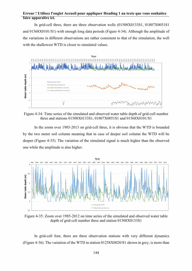
Erreur ! Utilisez l'onglet Accueil pour appliquer Heading 1 au texte que vous souhaitez faire apparaître ici.
144
In grid-cell three, there are three observation wells (01508X0133S1, 01807X0051S1
and 01568X0101/S1) with enough long data periods (Figure 4-34). Although the amplitude of
the variations in different observations are rather consistent to that of the simulation, the well
with the shallowest WTD is closer to simulated values.
Figure 4-34: Time series of the simulated and observed water table depth of grid-cell number
three and stations 01508X0133S1, 01807X0051S1 and 01568X0101/S1
In the zoom over 1985-2013 on grid-cell three, it is obvious that the WTD is bounded
by the two meter soil column meaning that in case of deeper soil column the WTD will be
deeper (Figure 4-35). The variation of the simulated signal is much higher than the observed
one while the amplitude is also higher.
Figure 4-35: Zoom over 1985-2012 on time series of the simulated and observed water table
depth of grid-cell number three and station 01508X0133S1
In grid-cell four, there are three observation stations with very different dynamics
(Figure 4-36). The variation of the WTD in station 01258X0020/S1 shown in grey, is more than
0
2
4
6
8
10
12
1960
1960
1961
1962
1963
1964
1965
1965
1966
1967
1968
1969
1970
1970
1971
1972
1973
1974
1975
1975
1976
1977
1978
1979
1980
1980
1981
1982
1983
1984
1985
1985
1986
1987
1988
1989
1990
1990
1991
1992
1993
1994
1995
1995
1996
1997
1998
1999
2000
2000
2001
2002
2003
2004
2005
2005
2006
2007
2008
2009
2010
2010
2011
2012
2013
2014
2015
2015
Simulation WTD
Observed Less than 2 m
Observed between 2 and 10 m
Observed between 10 and 20 m
Wat
er ta
ble
dept
h (m
)
Year
0
0.5
1
1.5
2
2.5
1985 1986 1987 1988 1989 1990 1991 1992 1993 1994 1995 1996 1997 1998 1999 2000 2001 2002 2003 2004 2005 2006 2007 2008 2009 2010 2011 2012 2013Chart Title
Simulation WTD
Observed Less than 2 m
Wat
er ta
ble
dept
h (m
)
Year

Erreur ! Utilisez l'onglet Accueil pour appliquer Heading 1 au texte que vous souhaitez faire apparaître ici.
145
10 meters within the data period, which can be linked to the Karstic nature of the aquifer,
interaction with a confined layer or extensive exploitations.
Figure 4-36: Time series of the simulated and observed water table depth of grid-cell number four and stations 01258X0020/S1, 01516X0021/S1 and 01022X0073/P
In grid-cell four, although there is phase difference for the peaks and lows of the
simulated and observed water table depth in station 01022X0073/P, the overall dynamic and
variation of the simulated water table is similar to the observed one with almost one meter of
difference.
Figure 4-37: Zoom over 2007-2016 on the time series of the simulated and observed water table depths near Beauvais, grid-cell number four and station 01022X0073/P
0
5
10
15
20
25
1960
1962
1964
1966
1968
1970
1972
1974
1976
1978
1980
1982
1984
1986
1988
1990
1992
1994
1996
1998
2000
2002
2004
2006
2008
2010
2012
2014
Simulated WTD
Observed between 2 and 10 m
Observed between 10 and 20 m
Observed more than 20 m
Wat
er ta
ble
dept
h (m
)
Year
y = 0.0032x + 1.1912
y = 0.0029x + 3.7399
0
0.5
1
1.5
2
2.5
3
3.5
4
4.5
5
2007 2008 2009 2010 2011 2012 2013 2014 2015
Simulated WTD
Observed between 2 and 10 m
Year
Wat
er ta
ble
dept
h (m
)

Erreur ! Utilisez l'onglet Accueil pour appliquer Heading 1 au texte que vous souhaitez faire apparaître ici.
146
In this zone, although the simulated and observed water table depths are different in
dynamics and the correlation coefficient is low (0.13), the mean decline of the water table depth
is captured correctly by the model around -3 millimeters per month.
In grid-cell five, there are also three observation wells, with different water table depth
ranges. The shallowest observed water table depth is in 01518X0139/FE2 (shown in red in
Figure 4-39) with a mean WTD around 6 meters. The variation of the observed WTD is higher
for shallow aquifers compared to the deep aquifer of 01516X0004/S1 (shown in yellow). This
is because the connection between atmosphere and groundwater is weaker for the deep aquifer
and the variation of the WTD is less affected by the seasonal atmospheric changes.
Figure 4-38: Time series of the simulated and observed water table depth in grid-cell five and stations 01518X0139/FE2, 01516X0004/S1 and 02173X0008F
The model however is not capable of capturing the seasonality of the water table depth
correctly in zones of alluvial plains where the water table depth variations are affected by the
seasonality of the incoming precipitation and atmospheric evaporation demand. For example,
in La Bassée floodplains (grid-cell number eleven), upstream of the confluence of Yonne and
Seine, the shallow water table around three meters deep is highly affected by the surface
variables and is considerably seasonal (Figure 4-39). Shallow water table depth observations
(shallower than two meters) do not show the seasonal variations and the simulated water table
depth is more variant.
0
5
10
15
20
25
30
35
1960
1961
1962
1963
1964
1965
1967
1968
1969
1970
1971
1972
1974
1975
1976
1977
1978
1979
1981
1982
1983
1984
1985
1986
1988
1989
1990
1991
1992
1993
1995
1996
1997
1998
1999
2000
2002
2003
2004
2005
2006
2007
2009
2010
2011
2012
2013
2014
Simulate WTD
Observed between 2 and 10 m
Observed between 10 and 20 m
Observed more than 20 m
Wat
er ta
ble
dept
h (m
)
Year

Erreur ! Utilisez l'onglet Accueil pour appliquer Heading 1 au texte que vous souhaitez faire apparaître ici.
147
Figure 4-39: The time series of the simulated and observed water table depth near La Bassée floodplain, grid-cell number eleven and stations 02606X0125/PM3,
02605X0062/M4,02953X0089/S2,02606X1013/S1 and 02606X0120/FG1
This is also the case for grid-cell number six over the floodplains of the Oise River, where the
seasonality of the water table depth in the range between 10 to 20 meters is of the order of a
few meters, while the simulated WTD only varies between zero to two meters (Figure 4-40).
Figure 4-40: The time series of the simulated and observed water table depth near the Oise River over 1974 to 1983, grid-cell number six and station 01272X0086/S1
In grid-cells where there is little or no observation of the water table depth within the rather
shallow ranges, the observations of deep aquifers can be comparable to simulations if the
aquifer is unconfined. This is the case for grid-cell number seven near Paris where the
observation of the WTD varies within a two meter range (Figure 4-42). This is an evidence for
0
2
4
6
8
10
12
14
16
18
1998 1999 2000 2001 2002 2003 2004
Simulated WTDObservation less than 2 metersObservation between 2 and 10 mObservation between 2 and 10 mObservation between 2 and 10 mObservation between 2 and 10 mObservation between 10 and 20 mObservation more than 20 m
Wat
er ta
ble
dept
h (m
)Years
0
5
10
15
20
25
1974 1975 1976 1977 1978 1979 1980 1981 1982 1983
Simulated WTD
Observed between 10 and 20 m
Year
Wat
er ta
ble
dept
h (m
)

Erreur ! Utilisez l'onglet Accueil pour appliquer Heading 1 au texte que vous souhaitez faire apparaître ici.
148
the fact that even deep water tables can be affected by the surface conditions and vary with
seasonal changes of the atmosphere.
Figure 4-41: The time series of the simulated and observed water table depth near Paris area for simulated and deep observed water table depths for the simulation data period, grid-cell
number seven and stations 01834A0153/PZ1 and 01837B0380/F1
Figure 4-42: The time series of the simulated and observed water table depth near Paris area for simulated and deep observed water table depths for the period 1985 to 1995, grid-cell
number seven and station 01837A0096/F2
The WTD in the rest of the grid-cells is also in relative similarity with the observed
ones, while significant differences between the simulation and observation are sometimes
detected. In almost all examples the observed water table depth is deeper than 2 meters and
therefore deeper than simulations. The comparison is based on the variation of the WTD in
simulated and observed examples. The time series of the WTD in these grid-cells is presented
in Figure 4-43 to Figure 4-45.
0
5
10
15
20
25
30
35
1960
1962
1964
1966
1968
1970
1972
1974
1976
1978
1980
1982
1984
1986
1988
1990
1992
1994
1996
1998
2000
2002
2004
2006
2008
2010
2012
2014
Simulate WTDObserved less than 2 mObserved between 2 and 10 mObserved between 10 and 20 mObserved more than 20 mObserved more than 20 mW
ater
tabl
e de
pth
(m)
Observed between 2 and 10 m
Observed more than 20 m
0
5
10
15
20
25
30
1985 1986 1987 1988 1989 1990 1991 1992 1993 1994 1995
Observed more than 20 m
Simulate WTD
Year
Wat
er ta
ble
dept
h (m
)

Erreur ! Utilisez l'onglet Accueil pour appliquer Heading 1 au texte que vous souhaitez faire apparaître ici.
149
Figure 4-43: The time series of the simulated and observed water table depth in grid-cell number eight for simulated and observed water table depths for the simulation period. WTD
observation wells: 01287X0017/S1, 01042X0049/S1 and 01045X0015/S1
Figure 4-44: The time series of the simulated and observed water table depth in grid-cell number nine for simulated and observed water table depths for the simulation period. WTD
observation wells: 02206X0085/F, 02206X0030/S1, 02582X0268 and 02203X0106/P3
0
5
10
15
20
25
1960
1962
1964
1966
1968
1970
1972
1974
1976
1978
1980
1982
1984
1986
1988
1990
1992
1994
1996
1998
2000
2002
2004
2006
2008
2010
2012
2014
Simulated WTDObserved less than 2 mObserved between 2 and 10 mObserved between 10 and 20 mObserved between 10 and 20 mObserved more than 20 m
Observed between 10 and 20 mObserved more than 20 m
Wat
er ta
ble
dept
h (m
)Year
0
5
10
15
20
25
30
35
40
45
50
1960
1960
1961
1962
1963
1964
1965
1966
1967
1968
1969
1970
1971
1971
1972
1973
1974
1975
1976
1977
1978
1979
1980
1981
1982
1982
1983
1984
1985
1986
1987
1988
1989
1990
1991
1992
1993
1993
1994
1995
1996
1997
1998
1999
2000
2001
2002
2003
2004
2004
2005
2006
2007
2008
2009
2010
2011
2012
2013
2014
2015
2015
Simulation WTDObserved less than 2 mObserved between 2 and 10 mObserved between 10 and 20 mObserved more than 20 mObserved more than 20 m
Wat
er ta
ble
dept
h (m
)
Year

Erreur ! Utilisez l'onglet Accueil pour appliquer Heading 1 au texte que vous souhaitez faire apparaître ici.
150
Figure 4-45: The time series of the simulated and observed water table depth in grid-cell number ten for simulated and observed water table depths for the simulation period. WTD
observation wells: 02582X0269/P17, 02581X0104/P18 and 02943X0013/S1
4.7.2 Comparison against GRACE gravity measurements
Here, since the GRACE measurements are at one degree resolution, the same
ORCHIDEE simulation were performed at this resolution for better comparisons. The
simulation named ORCHIDEE-WET here is with a two meter soil column depth, exchange
factor set to 1000 and wetland fractions read from CW-WTD map. The anomalies of the TWS
in ORCHIDEE appears to be well in-phase with respect to those of GRACE (Figure 4-46).
Many peaks and lows are correctly modelled in ORCHIDEE particularly within the second half
of the GRACE data history. The GRACE anomaly monthly values, which is the average of
three solutions for TWS (section 4.3), does not have a regular time sequence and includes some
gaps within the months. Here for the sake of visual simplicity, GRACE measurements are
shown with a line in Figure 4-46 and each two consecutive reading is connected with a line
between them.
The difference between ORCHIDEE-REF and ORCHIDEE-WET is slight. This
difference is more pronounced over the peaks where the ORCHIDEE-WET appears to be less
variant. terrestrial water storage peaks are where the reservoirs are full which is often during
the wet season. Increased evapotranspiration (because of the shallow water table) during the
wet season in ORCHIDEE-WET causes the TWS to drop down slightly in comparison to
ORCHIDEE-REF. Also during the dry seasons, simulated TWS in ORCHIDEE-WET is higher
0
5
10
15
20
25
1960
1962
1964
1966
1968
1970
1972
1974
1976
1978
1980
1982
1984
1986
1988
1990
1992
1994
1996
1998
2000
2002
2004
2006
2008
2010
2012
2014
Simulated WTD
Observed between 10 and 20 m
Observed more than 20 m
Wat
er ta
ble
dept
h (m
)Year

Erreur ! Utilisez l'onglet Accueil pour appliquer Heading 1 au texte que vous souhaitez faire apparaître ici.
151
than ORCHIDEE-REF because of the buffer effect of the wetlands and accumulated water in
the wetland soil column.
Figure 4-46: Comparison of the total Terrestrial Water Storage in GRACE observations and monthly precipitations, ORCHIDEE-REF and ORCHIDEE-WET
4.8 Conclusion
The inclusion of the groundwater and wetlands in the ORCHIDEE platform is of great
importance for analyzing the effect of subsurface-surface interactions in the Earth system.
ORCHIDEE-WET considers the wetland (lowland) fraction as the soil-tile which receives
water fluxes not only from precipitation but also from the non-wetland (upland) fraction of the
grid-cell. In this way, if the water fluxes are enough, a water table is built in the wetland fraction
leading to increased evapotranspiration and water flux from groundwater and the streams. If
there is water excess, so that the soil-tile column fills up completely, the entering water fluxes
are directly diverted to surface runoff.
This chapter was focused on different tests regarding parameters of the groundwater and
fluxes and analyzing the ORCHIDEE-WET as compared to ORCHIDEE-REF versions. First
the ORCHIDEE-REF version was tested for varying atmospheric forcings and reservoir time
constants. After deciding on these parameters the behavior of ORCHIDEE-WET was analyzed
for different exchange rates, wetland fractions and soil depths.
Anom
aly
of T
WS
(cm
)Precipitation (m
m/day)
0
2
4
6
8
10
12
14
-20
-15
-10
-5
0
5
10
15
20
2002 2003 2004 2005 2006 2007 2008 2009 2010 2011 2012 2013 2014
Prec
GRACE
ORC-REF
ORC-WET
Year

Erreur ! Utilisez l'onglet Accueil pour appliquer Heading 1 au texte que vous souhaitez faire apparaître ici.
152
It was shown that the CRU-NCEP set of atmospheric forcings gives the best results for
simulations overs the Seine River basin. Also, since adjusting the reservoir time-constants
requires a separate calibration procedure the default values of constants (calibrated over the
Senegal basin by Ngo-Duc et al. 2007) were used for further simulations. Adjusting reservoir
time constants and exchange factors in a calibration procedure for each set of atmospheric
forcings can be a perspective to this study.
In ORCHIDEE-WET the exchange factor between the groundwater and the stream
affects the seasonality of the river discharge considerably. While using low exchange factors
leads to an advanced river discharge with very low dry seasons discharge, increasing this factor
tends to smoothen the monthly flows and intensifying the buffer effect of wetlands.
The potential wetland fraction can be very varying over different regions of the Earth.
But depending on the amount of entering fluxes to these potential wetland fractions, the water
table may or may not form. For example, over the Seine River basin, a 5% wetland percentage
is completely possible during the whole year having the definition of wetlands with water table
depth shallower than 20 cm. But a 25% wetland fraction is only realizable during the winter
months and for the rest of the year the water table goes deeper. In all cases since the groundwater
approaches the surface, the evapotranspiration rates increase. Increased wetland fraction also
translates into smaller upland fraction and drainage. Since the bottom drainage is blocked in
ORCHIDEE-WET lowland soil-tile, when there is excess of water in the wetland soil column,
the water directly goes to nearby streams without a retention time. This is why the winter time
river discharge is higher for higher wetland fraction and the summer time discharge drops
downs when the wetland fraction is increased.
The parameter with the most sensitivity over the surface variables is the soil depth. In
the default ORCHIDEE versions, the soil depth is set to two meters. The effect of deeper soil
columns was tested. When the soil depth is increased, the soil column gradually becomes a very
large leaky bucket. It means that the water accumulates in the deep soil column with the outflux
being only the fluxes from the groundwater and the stream. For example, increasing the soil
depth beyond 10 meters appears to have very little effect on the stream flow since the discharge
becomes almost constant when soil depth is increased more than this threshold. It appear that
the soil column depth should be different for upland and lowland (shallower soil depth for
upland and deeper for wetlands) to better simulate the water exchange between these two

Erreur ! Utilisez l'onglet Accueil pour appliquer Heading 1 au texte que vous souhaitez faire apparaître ici.
153
partitions of the grid-cell. This assumption is a valid one since the soil thickness is thinner in
the steep uplands compared to lowlands were all alluvial deposits are.
The effect of the existing groundwater parametrization in ORCHIDEE-REF through the
time constants in the routing scheme was to delay the discharge and decrease the amplitude of
the seasonal variations of the flow. In contrast, the effect of the hillslope hydrology in
ORCHIDEE-WET is in the opposite direction through decreasing the overall river discharge,
advancing the flow and increasing the amplitude of discharge variations. This points toward a
non-linearity of the groundwater effect in the lowland fractions which is frequently observed
(Chapman, 1999; Eltahir and Yeh, 1999; Troch et al., 2003).
Generally the simulated water table depth with ORCHIDEE-WET with the two meter
soil depth are comparable to observed water table depths of the same order. Also, since the
resolution of the ORCHIDEE simulation is low, we have only one time-serie of water table
depths for the lowland fraction of each grid-cell of size 0.5°× 0.5° (almost 39 km×50 km for
the Seine River basin) to be compared with observed values. The dynamic of the simulated
water table depth throughout the year is often more varying than that of the observations. Only
at some instances the simulated and observed water table depths are comparable. On the other
hand, the time-series of the terrestrial water storage anomaly for ORCHIDEE-WET and
ORCHIDEE-REF are very similar to GRACE observations, particularly within the period
2006-2012. As a result, because of the coarse resolution of ORCHIDEE, it is suggested that for
comparisons of the ORCHDEE-GW with observations GRACE measurements can be of more
interest than the well observations.
Among the surface and subsurface variables like evaporation, precipitation,
groundwater level and river flow, almost all but the precipitation follow the seasonal variations
over the Seine River basin. As suggested by Eltahir and Yeh (1999), because of the slow nature
of the water movement within the soil, the seasonal cycle of the groundwater level is similar to
that of soil moisture with a lag. This shows the clear signature of evapotranspiration (driven by
the solar radiation) in shaping the climatology of subsurface variables in the Seine River basin.

Erreur ! Utilisez l'onglet Accueil pour appliquer Heading 1 au texte que vous souhaitez faire apparaître ici.
154
Chapter 5
Conclusions and perspectives
In this chapter, the issues of the previous chapters are first summarized and then some
concluding remarks are discussed. This discussion is categorized into two main sections,
following the different chapters of the thesis. One discusses all the aspects of the wetland
mapping at the global scale and the other mostly explains the modelling effort to include
wetlands in the ORCHIDEE climate model. At the end, perspectives are provided.
5.1 The potential wetland distribution
The potential wetland distribution in contrast to actual wetland distribution is more
applicable in wetland modeling since the extent of wetlands is variable within the different
months of the year, and also helps analyzing the effect of human interaction in draining the
wetlands. The other point is that, even in zones with not very shallow water table (around 1
meter), there is a sensible effect of wetlands through the increased evapotranspiration from the
wetland soil-tile with respect to reference simulations. This points out the necessity to have a
broader definition for wetlands and their mapping as areas with significant interaction between
groundwater and atmosphere.
In this study, the potential wetland distribution is derived from overlaying the products
of surface water imagery and simple groundwater modellings. This enables not only capturing
the regularly flooded wetlands but also the groundwater driven ones. To this end, surface water
maps of ESA-CCI, GIEMS-D15 and JRC are superposed with each other and also groundwater-
fed wetland derived either from direct groundwater modelling of Fan et al. (2013) or indirect
modelling of topo-climatic index. These potential wetland maps cover almost 20% of the land
surface of the Earth.

Erreur ! Utilisez l'onglet Accueil pour appliquer Heading 1 au texte que vous souhaitez faire apparaître ici.
155
Wetlands in the developed maps have higher density over the northern Canadian region,
western Siberia, Amazon basin, tropical Africa, south and south-east Asia than other regions of
the world. In northern regions, the high density of wetlands is caused by low evapotranspiration
rates; while in tropical and subtropical regions, high wetland density is derived from excessive
precipitation rates and flat slopes.
The wetlands in the composite wetland maps are larger than most wetland datasets
including the GLWD (Lehner and Döll, 2004). But these high densities are confirmed through
regional validations, particularly over France (in comparison to MPHFM: Berthier et al., 2014).
It should be emphasized that recent studies on the extent and distribution of potential wetlands
at the global scale estimate the wetland fraction to be between 15-21% of the land surface area
(Fan et al., 2013; Hu et al., 2017; Aires et al., 2018).
The developed wetland map in the next step is used as a land feature to be forced into
the hydrological model as the lowland fraction (soil-tile). In each grid-cell, wetlands are the
zones where the groundwater (flow from the slow reservoir) converges and builds up a water
table, connecting the groundwater with the atmosphere (if the water table is shallow enough).
The wetlands of the developed maps are categorized based on their water sources into
regularly flooded wetlands (RFWs) and groundwater driven wetlands (GDWs), but they are not
classified based on their environmental functions into different classes.
5.2 Modelling groundwater flow and wetlands in land surface models
Modelling groundwater on the platform of a land surface model has been rarely done in
the literature. In this study, we integrated the groundwater into the ORCHIDEE land surface
model by defining a water flux mechanism that drives drained water in the upland to the wetland
fraction. The wetland fraction itself interacts with surface and streams through the water table
as well. Although groundwater modelling at fine resolution often requires detailed maps of soil
texture, aquifer depth and hydrodynamic properties of the subsurface, this is a first effort
towards integrating the subsurface medium into land surface models at the coarse resolution
with limited information. It is important at this step to capture the main dynamics of
groundwater flow with different seasons and the effect of wetlands as the interface between the
subsurface resources and surface elements. Since there are multiple simplistic assumptions in
ORCHIDEE-WET like the blocked bottom drainage of the wetlands (water drains laterally),

Erreur ! Utilisez l'onglet Accueil pour appliquer Heading 1 au texte que vous souhaitez faire apparaître ici.
156
river bed level, and constant soil column for upland and lowland, the output surface variables
might not be readily comparable to observations. This is why the comparison of the simulated
and observed water table depths, for example, are limited to shallow observations. However,
the river discharges with the ORCHIDEE-WET are closer to observations than that of
ORCHIDEE-REF with advanced flows toward winter and minimum flows (too low) around
August and September, similar to ORCHIDEE-REF simulation with small time constants and
observations. This is interesting because the hillslope hydrology defined for the wetland
element advances the flow instead of delaying it. Adding the hillslope hydrology to the existing
parametrization of the groundwater with a linear slow reservoir in ORCHIDEE leads to a non-
linear effect of groundwater on the river flow.
When the simulated terrestrial water storage is compared to GRACE measurements,
there is a considerable resemblance between the anomaly of the TWS in simulation (both
ORCHIDEE-REF and ORCHIDEE-WET) and observation. The buffer effect of wetlands is
observed in the TWS comparison between ORC-REF and ORC-WET, where the variations in
ORC-WET is slightly smaller than ORC-REF.
5.3 Perspectives
This study, particularly the part with the ORCHIDEE modifications to adapt for
integrating the groundwater, is a first attempt towards developing a comprehensive land surface
model with an explicit representation of the surface-subsurface interactions. As a result, there
are many additional steps that can be imagined to generate a more physically-based model.
First of all, we developed here a comprehensive wetland map extending the existing
definitions for wetlands. This new effort resulted in wetland fractions that are equal or
sometimes greater than existing examples. In order to integrate this wetland map into land
surface modeling, different classes of wetland should be defined. In this way, we could develop
specific hydrologic processes for each type of wetlands. For example, the coastal wetlands are
sometimes fed by the sea water during the high tide and drained during the low tide. As a result
they not only interact with the groundwater, but also they are co-related with the sea level rise
and falls. In the present wetland map and hydrologic mechanism, all wetlands are assumed to
interact with rivers and also they are defined to be within the lowlands. However, isolated
wetlands may occur in zones with no interaction with streams (tidal wetlands) and also within
the uplands.

Erreur ! Utilisez l'onglet Accueil pour appliquer Heading 1 au texte que vous souhaitez faire apparaître ici.
157
In the simulation step of the study, we noticed that the ORCHIDEE simulation results
for the surface variables are highly sensitive to reservoirs time-constants. As mentioned in the
manuscript, in its current version, ORCHIDEE uses a previously calibrated set of reservoir time
constants over the Senegal Basin (Ngo-Duc et al., 2007). Senegal River has a highly seasonal
flow with very low summer time discharge rates (mean maximum flow during October: 2250
m3/s, mean minimum flow during May: 60 m3/s). Using these calibrated parameters in other
basins of the world may result in inaccurate river discharges. Additionally, calibrating the time-
constants for all of the basin is very time-consuming and is contradictory to the objective of
physically-based modelling the Earth system. Schneider et al. (2017) extracted the river
network density globally and calculated the base flow time constant (slow reservoir time
constant) from the drainage density and aquifer transmissivity.
The exchange factor (EF) of the ORCHIDEE-WET allows to modulate the residence
time of the lowland fraction: since the flow from the lowland fraction to river increases with
EF, the larger the EF, the smaller the residence time. This is also connected to the buffer effect
of the wetlands. By lowering the exchange factor, the residence time increases and hence the
buffer effect. On the other hand, by reducing the base-flow (through EF) the lowland soil
moisture increases which enhances the surface runoff, opposing the buffer effect on streamflow.
Therefore, interesting test simulations could be a simulation with ORC-WET (soil depth=5m,
EF=1), in which the soil column should be humid even for deep soil depths because of the small
EF.
The soil column depth in the default ORCHIDEE simulations is assumed to be two
meters. This constant soil column depth is assumed following tests that show that most of the
hydrological interaction between atmosphere and soil moisture happens within the first two
meters of the soil column (Campoy et al., 2013). But when subsurface mechanisms are added,
the interaction between groundwater, soil moisture and surface variables can take place in deep
layers of tens of meters depth. However, the effective soil depth is very different in various
parts of the world (Pelletier et al., 2016). Where soil layer is thin like in the mountainous regions
the modelled soil depth can be kept for two meters; but in alluvial plains and very dry regions,
the groundwater/surface exchanges can happen tens of meters down. As a result, the soil column
depth should be set as a forcing globally and read from a soil depth map to obtain better
simulations of the subsurface/surface interactions. Also, at least at the scale of the Seine River

Erreur ! Utilisez l'onglet Accueil pour appliquer Heading 1 au texte que vous souhaitez faire apparaître ici.
158
basin, a thorough calibration of the model parameter in ORCHIDEE-WET is required involving
time constants, soil depths and forcings.
In addition to geographically changing soil column depths over the world, soil depths
should be taken different for uplands and lowlands. As seen in Chapter 4, changing the model
soil depth deeper than 10 meters resulted in a constant river flow within the year in the Seine
River basin. Assuming very deep soil column depths for uplands in each grid-cell results in a
rather smooth and constant drainage from the bottom of the upland fraction which is then
redirected to be inserted in wetland fraction. Therefore, there should be a difference in depth
for uplands and lowlands where uplands, which are often located in steep areas, having a
shallow soil depths and lowlands (wetlands) having deep soil columns due to accumulation of
the sedimentary deposits in these areas. The exception to the latter can be the upland plateaus.
There are not many examples of studies on global soil depths and sometimes they are simply
calculated based on the land slope (Fan et al., 2013). Also, more sophisticated estimates of the
soil and sedimentary deposit depths are available with classification of soil, regolith and
sedimentary deposits which can help better differentiate between different surface mediums
(Pelletier et al., 2016).
We performed tests over the rather small region of the Seine River basin. In such small
extents, effects and feedbacks of wetlands on climate are not easily detected. Performing tests
over one of the wetland hotspots (discussed in Chapter 3) would help us better understand the
effect of climate change on wetlands (increased evapotranspiration or wetland drying). All tests
in this thesis were performed in offline configuration (not coupled with the atmospheric
module) so the feedback effect of wetlands on climate is not detectable.
Another perspective to this research is to activate the floodplain parametrization of
D’Orgeval et al. (2008) in addition to the wetland component of the ORCHIDEE-WET.
However it is suggested to read the floodplain extent from the RFW map composed in this study
(Chapter 3) and to add a surface storage for the excess water of the soil column in the lowland
fraction. This is because the excess water from the soil column in the current version of the
ORCHIDEE-WET is directly transferred to the river. Then, as a function of the soil wetness in
lowlands the methane emission from the wetlands could be more precisely estimated.
Although wetlands are important sources of methane emission to atmosphere (Dean et
al., 2018), the biogeochemical effect of wetlands is not discussed in this thesis. With the climate
Erreur ! Utilisez l'onglet Accueil pour appliquer Heading 1 au texte que vous souhaitez faire apparaître ici.
159
change and changes in the precipitation rate in different regions, the extent of wetlands and
their chemical activity may evolve with time. Developing a dynamic geochemical module for
wetland evolution based on precipitation and temperature changes is important for future
estimation of carbon emission from these land features.

Erreur ! Utilisez l'onglet Accueil pour appliquer Heading 1 au texte que vous souhaitez faire apparaître ici.
160

Erreur ! Utilisez l'onglet Accueil pour appliquer Heading 1 au texte que vous souhaitez faire apparaître ici.
161
Bibliography Abramopoulos, F., Rosenzweig, C. and Choudhury, B.: Improved Ground Hydrology
Calculations for Global Climate Models (GCMs): Soil Water Movement and
Evapotranspiration, J. Clim., 1(9), 921–941, 1988.
Acreman, M. and Holden, J.: How wetlands affect floods, Wetlands, doi:10.1007/s13157-
013-0473-2, 2013.
Adam, L., Döll, P., Prigent, C. and Papa, F.: Global-scale analysis of satellite-derived time
series of naturally inundated areas as a basis for floodplain modeling, Adv. Geosci., 27, 45–
50, doi:10.5194/adgeo-27-45-2010, 2010.
Adamus, P. . and Stockwell, L. T.: A method for wetland functional assessment: Volume 1
critical review and evaluation., 1983.
Aires, F., Miolane, L., Prigent, C., Pham, B., Fluet-Chouinard, E., Lehner, B. and Papa, F.: A
Global Dynamic Long-Term Inundation Extent Dataset at High Spatial Resolution Derived
through Downscaling of Satellite Observations, J. Hydrometeorol., 18(5), 1305–1325,
doi:10.1175/JHM-D-16-0155.1, 2017.
Aires, F., Prigent, C., Fluet-Chouinardm, E., Yamazaki, D., Papa, F. and Lehner, B.:
Comparison of visible and multi-satellite global inundation datasets at high-spatial resolution,
Remote Seinsing Environ., 216, 427–441, doi:https://doi.org/10.1016/j.rse.2018.06.015, 2018.
Barling, R. D., Moore, I. D. and Grayson, R. B.: A quasi‐dynamic wetness index for
characterizing the spatial distribution of zones of surface saturation and soil water content,
Water Resour. Res., 30(4), 1029–1044, doi:10.1029/93WR03346, 1994.
Bartholomé, E. and Belward, A. S.: GLC2000 : a new approach to global land cover mapping
from Earth observation data, Int. J. Remote Sens., 26(9), 1959–1977,
doi:10.1080/01431160412331291297, 2005.
Belward, A. S., Estes, J. E. and Kline, K. D.: The IGBP-DIS Global 1-km Land-Cover Data
Set DISCover: A Project Overview , Photogramm. Eng. Remote Sensing, Spec. issue Glob. L.
Cover data set Valid., 65(9), 1013–1020, 1999.
Bendjoudi, H., Weng, P., Guérin, R. and Pastre, J. F.: Riparian wetlands of the middle reach

Erreur ! Utilisez l'onglet Accueil pour appliquer Heading 1 au texte que vous souhaitez faire apparaître ici.
162
of the Seine river (France): Historical development, investigation and present hydrologic
functioning. A case study, J. Hydrol., 263(1–4), 131–155, doi:10.1016/S0022-
1694(02)00056-2, 2002.
Berthier, L., Bardy, M., Chenu, J. ., Guzmova, L., Laroche, B., Lehmann, S., Lemercier, B.,
Martin, M., Mérot, P., Squividant, H., Thiry, E. and Walter, C.: Enveloppes des milieux
potentiellement humides de la France métropolitaine - notice d’accompagnement. [online]
Available from: http://geowww.agrocampus-ouest.fr/metadata/pdf/Notice_MPH_France.pdf,
2014.
Beven, K. J. and Kirkby, M. J.: Physically based, variable contibution area model of basin
hydrology, Hydrol. Sci. Bull., 24(1), 43–69, doi:10.1080/02626667909491834, 1979.
Bierkens, M. F. P. and van den Hurk, B. J. J. M.: Groundwater convergence as a possible
mechanism for multi-year persistence in rainfall, Geophys. Res. Lett., 34(2), 1–5,
doi:10.1029/2006GL028396, 2007.
Billen, G. and Garnier, J.: Nitrogen transfers through the Seine drainage network : a budget
based on the application of the ‘ Riverstrahler ’ model, in Man and River Systems, pp. 139–
150, Springer Netherlands., 1999.
Billen, G., Garnier, J. and Hanset, P.: Modelling phytoplankton development in whole
drainage networks: the RIVERSTRAHLER Model applied to the Seine river system,
Hydrobiologia, doi:10.1007/BF00007414, 1994.
Boé, J., Terray, L., Habets, F. and Martin, E.: Statistical and dynamical downscaling of the
Seine basin climate for hydro-meteorological studies, Int. J. Climatol., 27(12), 1643–1655,
doi:10.1002/joc.1602, 2007.
Bohn, T. J., Lettenmaier, D. P., Sathulur, K., Bowling, L. C., Podest, E., McDonald, K. C. and
Friborg, T.: Methane emissions from western Siberian wetlands: Heterogeneity and sensitivity
to climate change, Environ. Res. Lett., 2(4), doi:10.1088/1748-9326/2/4/045015, 2007.
Bontemps, S., Herold, M., Kooistra, L., Van Groenestijn, A., Hartley, A., Arino, O., Moreau,
I. and Defourny, P.: Revisiting land cover observation to address the needs of the climate
modeling community, Biogeosciences, doi:10.5194/bg-9-2145-2012, 2012.
Brix, H., Sorrell, B. K. and Lorenzen, B.: Are phragmites-dominated wetlands a net source or
net sink of greenhouse gases?, Aquat. Bot., 69(2–4), 313–324, doi:10.1016/S0304-
3770(01)00145-0, 2001.
Erreur ! Utilisez l'onglet Accueil pour appliquer Heading 1 au texte que vous souhaitez faire apparaître ici.
163
Brunner, P., Cook, P. G. and Simmons, C. T.: Hydrogeologic controls on disconnection
between surface water and groundwater, Water Resour. Res., doi:10.1029/2008WR006953,
2009.
Brutsaert, W.: Hydrology: an introduction. 3rd ed., 2008.
Buckingham, E.: Studies on the Movement of Soil Moisture, U.S. Dep. Agric. Burreau Soils,
38, 61, doi:10.1017/CBO9781107415324.004, 1907.
Bullock, A. and Acreman, M.: The role of wetlands in the hydrological cycle, Hydrol. Earth
Syst. Sci., doi:10.5194/hess-7-358-2003, 2010.
Burt, T. P. and Butcher, D. P.: Development of topographic indices for use in semidistributed
hillslope runoff models, in Geomorphology and Land Management, pp. 1–19., 1986.
Campoy, A., Ducharne, A., Cheruy, F., Hourdin, F., Polcher, J. and Dupont, J. C.: Response
of land surface fluxes and precipitation to different soil bottom hydrological conditions in a
general circulation model, J. Geophys. Res. Atmos., 118(19), 10725–10739,
doi:10.1002/jgrd.50627, 2013.
Carson, D. J.: Current parametrizations of landsurface processes in atmospheric general
circulation models, in Proceedings of the JSC Study Conference on Land-Surface Processes
in Atmospheric General Circulation Models. WMO, pp. 67–108, WMO., 1982.
Chapman, T.: A comparison of algorithms for stream flow recession and baseflow separation,
Hydrol. Process., doi:10.1002/(SICI)1099-1085(19990415)13:5<701::AID-
HYP774>3.0.CO;2-2, 1999.
Chen, F. and Dudhia, J.: Coupling an Advanced Land Surface–Hydrology Model with the
Penn State–NCAR MM5 Modeling System. Part II: Preliminary Model Validation, Mon.
Weather Rev., 129(4), 587–604, doi:10.1175/1520-
0493(2001)129<0587:CAALSH>2.0.CO;2, 2001.
Cohen, M. J., Creed, I. F., Alexander, L., Basu, N. B., Calhoun, A. J. K., Craft, C., D’Amico,
E., DeKeyser, E., Fowler, L., Golden, H. E., Jawitz, J. W., Kalla, P., Kirkman, L. K., Lane, C.
R., Land, M., Leibowitz, S. G., Lewis, D. B., Marton, J., McLaughlin, D., Mushet, D. M.,
Raanan-Kiperwas, H., Rains, M. C., Smith, L. and Walls, S. C.: Do geographically isolated
wetlands influence landscape functions ?, PNAS, (February), doi:10.1073/pnas.1512650113,
2016.
Collins, W. J., Bellouin, N., Doutriaux-Boucher, M., Gedney, N., Halloran, P., Hinton, T.,
Erreur ! Utilisez l'onglet Accueil pour appliquer Heading 1 au texte que vous souhaitez faire apparaître ici.
164
Hughes, J., Jones, C. D., Joshi, M., Liddicoat, S., Martin, G., O’Connor, F., Rae, J., Senior,
C., Sitch, S., Totterdell, I., Wiltshire, A. and Woodward, S.: Development and evaluation of
an Earth-System model – HadGEM2, Geosci. Model Dev., 4(4), 1051–1075,
doi:10.5194/gmd-4-1051-2011, 2011.
Constance, E., Lauchlan, H., Mark, W., Szalay, D. and Ferenc, A.: Plant community
establishment in a restored wetland : Effects of soil removal, Appl. Veg. Sci., 10(3), 383–390,
2007.
Curie, F., Gaillard, S., Ducharne, A. and Bendjoudi, H.: Geomorphological methods to
characterise wetlands at the scale of the Seine watershed, Sci. Total Environ., 375(1–3), 59–
68, doi:10.1016/j.scitotenv.2006.12.013, 2007.
Curie, F., Ducharne, A., Bendjoudi, H. and Billen, G.: Spatialization of denitrification by
river corridors in regional-scale watersheds : Case study of the Seine river basin, Phys. Chem.
Earth, 36(12), 530–538, doi:10.1016/j.pce.2009.02.004, 2011.
D’Orgeval, T., Polcher, J. and De Rosnay, P.: Sensitivity of the West African hydrological
cycle in ORCHIDEE to infiltration processes, Hydrol. Earth Syst. Sci., 12(6), 1387–1401,
doi:10.5194/hess-12-1387-2008, 2008.
Dahle, C., Flechtner, F., Gruber, C., Konig, D., Konig, R., Michalak, G. and Neumayer, K.:
An Improved Time-Series of Monthly GRACE Gravity Field Solutions, Obs. Syst. Earth from
Sp., 29–39, doi:https://doi.org/10.1007/978-3-642-32135-1_4, 2014.
Darcy, H.: Les fontaines publique de la ville de Dijon, Victor Dalmont, Paris., 1856.
Dean, J. F., Middelburg, J. J., Röckmann, T., Aerts, R., Blauw, L. G., Egger, M., Jetten, M. S.
M., de Jong, A. E. E., Meisel, O. H., Rasigraf, O., Slomp, C. P., in’t Zandt, M. H. and
Dolman, A. J.: Methane Feedbacks to the Global Climate System in a Warmer World, Rev.
Geophys., 56(1), 207–250, doi:10.1002/2017RG000559, 2018.
Deardorff, J. W.: Efficient prediction of ground surface temperature and moisture, with
inclusion of a layer of vegetation, J. Geophys. Res., 83(C4), 1889,
doi:10.1029/JC083iC04p01889, 1978.
Desborough, C. E.: Surface energy balance complexity in GCM land surface models, Clim.
Dyn., 15(5), 389–403, doi:https://doi.org/10.1007/s003820050289, 1999.
Dhote, S. and Dixit, S.: Water quality improvement through macrophytes — a review,
Environ. Monit. Assess., 152(June 2008), 149–153, doi:10.1007/s10661-008-0303-9, 2009.

Erreur ! Utilisez l'onglet Accueil pour appliquer Heading 1 au texte que vous souhaitez faire apparaître ici.
165
Dickinson, R. E., Henderson-Sellers, A., Kennedy, P. J., Dickinson, E., Henderson-Sellers, A.
and Kennedy, J.: Biosphere-atmosphere Transfer Scheme (BATS) Version 1e as Coupled to
the NCAR Community Climate Model, NCAR Tech. Rep. NCAR/TN-3871STR, 72,
(August), 77, doi:10.5065/D67W6959, 1993.
Dingman, S.: Physical hydrology, third., Waveland press., 2015.
Dirmeyer, P. A., Gao, X., Zhao, M., Guo, Z., Oki, T. and Hanasaki, N.: GSWP-2: Multimodel
analysis and implications for our perception of the land surface, Bull. Am. Meteorol. Soc.,
87(10), 1381–1397, doi:10.1175/BAMS-87-10-1381, 2006.
Döll, P. and Fiedler, K.: Global-scale modeling of groundwater recharge, Hydrol. Earth Syst.
Sci., 12(3), 863–885, doi:10.5194/hess-12-863-2008, 2008.
Ducharne, A.: Reducing scale dependence in TOPMODEL using a dimensionless topographic
index, Hydrol. Earth Syst. Sci., 13(12), 2399–2412, doi:10.5194/hess-13-2399-2009, 2009.
Ducharne, A.: The hydrol module of ORCHIDEE : scientific documentation [ rev 1387 ] + [
rev 2419 ] for soil texture, , 1–30, 2014.
Ducharne, A., Laval, K. and Polcher, J.: Sensitivity of the hydrological cycle to the
parametrization of soil hydrology in a GCM, Clim. Dyn., 14(5), 307–327,
doi:10.1007/s003820050226, 1998.
Ducharne, A., Golaz, C., Leblois, E., Laval, K., Polcher, J., Ledoux, E. and De Marsily, G.:
Development of a high resolution runoff routing model, calibration and application to assess
runoff from the LMD GCM, J. Hydrol., doi:10.1016/S0022-1694(03)00230-0, 2003.
Ducharne, A., Baubion, C., Beaudoin, N., Benoit, M., Billen, G., Brisson, N., Garnier, J.,
Kieken, H., Lebonvallet, S., Ledoux, E., Mary, B., Mignolet, C., Poux, X., Sauboua, E.,
Schott, C., Théry, S. and Viennot, P.: Long term prospective of the Seine River system:
Confronting climatic and direct anthropogenic changes, Sci. Total Environ., 375, 292–311,
doi:10.1016/j.scitotenv.2006.12.011, 2007.
Ducharne, A., Ottlé, C., Maignan, F., Vuichard, N., Ghattas, J., Wang, F., Peylin, P., Polcher,
P., Guimberteau, M., Maugis, P., Tafasca, S., Tootchi, A., Verhoef, A. and Mizuachi, H.: The
hydrol module of ORCHIDEE: scientific documentation. [online] Available from:
http://forge.ipsl.jussieu.fr/orchidee/raw-
attachment/wiki/Documentation/UserGuide/eqs_hydrol.pdf, 2018.
Ducoudré, N. I., Laval, K. and Perrier, A.: SECHIBA, a New Set of Parameterizations of the

Erreur ! Utilisez l'onglet Accueil pour appliquer Heading 1 au texte que vous souhaitez faire apparaître ici.
166
Hydrologic Exchanges at the Land-Atmosphere Interface within the LMD Atmospheric
General Circulation Model, J. Clim., 6(2), 248–273, doi:10.1175/1520-
0442(1993)006<0248:SANSOP>2.0.CO;2, 1993.
Eltahir, E. A. B. and Yeh, P. J. F.: On the asymmetric response of aquifer water level to
floods and droughts in Illinois, Water Resour. Res., 35(4), 1199–1217,
doi:10.1029/1998WR900071, 1999.
Explore-2070: Hydrologie souterraine: Bassin de la Seine. [online] Available from:
https://professionnels.afbiodiversite.fr/sites/default/files/pdf/RE_Explore2070_Eaux_Sout_Zo
om_Seine.pdf, 2012.
Famiglietti, J. S. and Wood, E. F.: Application of multiscale water and energy balance models
on a tallgrass prairie, Water Resour. Res., 30(11), 3079–3093, 1994.
Fan, Y. and Miguez-Macho, G.: A simple hydrologic framework for simulating wetlands in
climate and earth system models, Clim. Dyn., 37(1), 253–278, doi:10.1007/s00382-010-0829-
8, 2011.
Fan, Y., Li, H. and Miguez-Macho, G.: Global Patterns of Groundwater Table Depth, Science
(80-. )., 339(6122), 940–943, doi:10.1126/science.1229881, 2013.
Fan, Y., Miguez-macho, G., Jobbágy, E. G., Jackson, R. B. and Otero-casal, C.: Hydrologic
regulation of plant rooting depth, in The National Academy of Sciences, vol. 114, pp. 10572–
10577., 2017.
Feng, M., Sexton, J. O., Channan, S. and Townshend, J. R.: A global, high-resolution (30-m)
inland water body dataset for 2000: first results of a topographic–spectral classification
algorithm, Int. J. Digit. Earth, 8947(July), 1–21, doi:10.1080/17538947.2015.1026420, 2015.
Finlayson, C. M., Davidson, N. C., Spiers, A. G. and Stevenson, N. J.: Global wetland
inventory – current status and future priorities, Mar. Freshw. Res., 50(8), 717,
doi:10.1071/MF99098, 1999.
Flipo, N.: Modélisation intégrée des transferts d’azote dans les aquifères et les rivières:
Application au bassin du Grand Morin, École Nationale Supérieure des Mines de Paris., 2005.
Flipo, N., Mouhri, A., Labarthe, B., Biancamaria, S., Rivière, A. and Weill, P.: Continental
hydrosystem modelling: The concept of nested stream–aquifer interfaces, Hydrol.
Earth Syst. Sci., 18(8), 3121–3149, doi:10.5194/hess-18-3121-2014, 2014.

Erreur ! Utilisez l'onglet Accueil pour appliquer Heading 1 au texte que vous souhaitez faire apparaître ici.
167
Fluet-Chouinard, E., Lehner, B., Rebelo, L. M., Papa, F. and Hamilton, S. K.: Development
of a global inundation map at high spatial resolution from topographic downscaling of coarse-
scale remote sensing data, Remote Sens. Environ., 158, 348–361,
doi:10.1016/j.rse.2014.10.015, 2015.
Frappart, F. and Ramillien, G.: Monitoring groundwater storage changes using the Gravity
Recovery and Climate Experiment (GRACE) satellite mission: A review, Remote Sens.,
10(6), doi:10.3390/rs10060829, 2018.
Freeze, R. A. and Witherspoon, P. A.: Theoretical analysis of regional groundwater flow: 1.
Analytical and numerical solutions to the mathematical model, Water Resour. Res., 2(4),
641–656, doi:10.1029/WR002i004p00641, 1966.
Friedl, M. A., Sulla-Menashe, D., Tan, B., Schneider, A., Ramankutty, N., Sibley, A. and
Huang, X.: MODIS Collection 5 global land cover: Algorithm refinements and
characterization of new datasets, Remote Sens. Environ., doi:10.1016/j.rse.2009.08.016,
2010.
Fritz, S. and See, L.: Comparison of land cover maps using fuzzy agreement, Int. J. Geogr.
Inf. Sci., 19(7), 787–807, doi:10.1080/13658810500072020, 2005.
Fuhrer, O., Chadha, T., Hoefler, T., Kwasniewski, G., Lapillonne, X., Leutwyler, D., Lüthi,
D., Osuna, C., Schär, C., Schulthess, T. C. and Vogt, H.: Near-global climate simulation at
1km resolution: Establishing a performance baseline on 4888 GPUs with COSMO 5.0,
Geosci. Model Dev., 11(4), 1665–1681, doi:10.5194/gmd-11-1665-2018, 2018.
Gedney, N. and Cox, P. M.: The Sensitivity of Global Climate Model Simulations to the
Representation of Soil Moisture Heterogeneity, J. Hydrometeorol., 4(6), 1265–1275,
doi:10.1175/1525-7541(2003)004<1265:TSOGCM>2.0.CO;2, 2003.
van Genuchten, M. T.: A Closed-form Equation for Predicting the Hydraulic Conductivity of
Unsaturated Soils1, Soil Sci. Soc. Am. J., 44(5), 892,
doi:10.2136/sssaj1980.03615995004400050002x, 1980.
Giorgi, F., Marinucci, M. R. and Bates, G. T.: Development of a Second-Generation Regional
Climate Model (RegCM2). Part I: Boundary-Layer and Radiative Transfer Processes, Mon.
Weather Rev., 121(10), 2794–2813, doi:10.1175/1520-
0493(1993)121<2794:DOASGR>2.0.CO;2, 1993.
Gleeson, T., Marklund, L., Smith, L. and Manning, A. H.: Classifying the water table at

Erreur ! Utilisez l'onglet Accueil pour appliquer Heading 1 au texte que vous souhaitez faire apparaître ici.
168
regional to continental scales, Geophys. Res. Lett., 38(5), 1–6, doi:10.1029/2010GL046427,
2011a.
Gleeson, T., Smith, L., Moosdorf, N., Hartmann, J., Dürr, H. H., Manning, A. H., Beek, L. P.
H. Van and Jellinek, A. M.: Mapping permeability over the surface of the Earth, Geophys.
Res. Lett., 38(January), 1–6, doi:10.1029/2010GL045565, 2011b.
Gleeson, T., Moosdorf, N., Hartmann, J. and van Beek, L. P. H.: A glimpse beneath earth’s
surface: GLobal HYdrogeology MaPS (GLHYMPS) of permeability and porosity, Geophys.
Res. Lett., 41(11), 3891–3898, 2014.
Gomez, E.: Modélisation intégrée de transfert de nitrate à l’échelle régionale dans un système
hydrologique, application au bassin de la Seine, Ecole Nationale Supérieure des Mines de
Paris., 2002.
De Graaf, I. E. M., Sutanudjaja, E. H., Van Beek, L. P. H. and Bierkens, M. F. P.: A high-
resolution global-scale groundwater model, Hydrol. Earth Syst. Sci., 19(2), 823–837,
doi:10.5194/hess-19-823-2015, 2015.
Grippa, M., Mognard, N. and Toan, T. Le: Comparison between the interannual variability of
snow parameters derived from SSM / I and the Ob river discharge, Remote Sens. Environ.,
98, 35–44, doi:10.1016/j.rse.2005.06.001, 2005.
Gruber, S.: The Cryosphere Derivation and analysis of a high-resolution estimate of global
permafrost zonation, Cryosph., 6(1), 221–233, doi:10.5194/tc-6-221-2012, 2012.
Guimberteau, M.: Modélisation de l’hydrologie continentale et influences de l’irrigation sur le
cycle de l’eau, University of Pierre and Marie Curie., 2010.
Gumbricht, T., Roman-Cuesta, R. M., Verchot, L., Herold, M., Wittmann, F., Householder,
E., Herold, N. and Murdiyarso, D.: An expert system model for mapping tropical wetlands
and peatlands reveals South America as the largest contributor, Glob. Chang. Biol.,
(February), doi:10.1111/gcb.13689, 2017.
Gurtz, J., Baltensweiler, A. and Lang, H.: Spatially distributed hydrotope-based modelling of
evapotranspiration and runoff in mountainous basins, Hydrol. Process., 13(17), 2751–2768,
doi:10.1002/(SICI)1099-1085(19991215)13:17<2751::AID-HYP897>3.0.CO;2-O, 1999.
Habets, F., Boone, A., Champeaux, J. L., Etchevers, P., Franchistéguy, L., Leblois, E.,
Ledoux, E., Le Moigne, P., Martin, E., Morel, S., Noilhan, J., Seguí, P. Q., Rousset-
Regimbeau, F. and Viennot, P.: The SAFRAN-ISBA-MODCOU hydrometeorological model

Erreur ! Utilisez l'onglet Accueil pour appliquer Heading 1 au texte que vous souhaitez faire apparaître ici.
169
applied over France, J. Geophys. Res. Atmos., 113(6), 1–18, doi:10.1029/2007JD008548,
2008.
Hagemann, S. and Dumenil, L.: A parametrization of the lateral waterflow for the global
scale, Clim. Dyn., doi:10.1007/s003820050205, 2002.
Haitjema, H. M. and Mitchell-bruker, S.: Are Water Tables a Subdued Replica of the
Topography ?, , 43(6), 781–786, doi:10.1111/j.1745-6584.2005.00090.x, 2005.
Hamilton, J. D., Kelly, C. A., Rudd, J. W. M., Hesslein, H. and Roulet, N. T.: Flux to the
atmosphere of CH4 and CO2 from wetland ponds on the Hudson Bay lowlands (HBLs), J.
Geophys. Res., 99(D1), 1495–1510, 1994.
Harris, I., Jones, P. D., Osborn, T. J. and Lister, D. H.: Updated high-resolution grids of
monthly climatic observations - the CRU TS3.10 Dataset, Int. J. Climatol., 34(3), 623–642,
doi:10.1002/joc.3711, 2014.
Hartmann, J. and Moosdorf, N.: The new global lithological map database GLiM: A
representation of rock properties at the Earth surface, Geochemistry, Geophys. Geosystems,
13(12), 1–37, doi:10.1029/2012GC004370, 2012.
Hattermann, F., Krysanova, V., Wechsung, F. and Wattenbach, M.: Integrating groundwater
dynamics in regional hydrological modelling, Environ. Model. Softw., 19(11), 1039–1051,
doi:10.1016/j.envsoft.2003.11.007, 2004.
Herbert, R.: Modelling Partially Penetrating Rivers on Aquifer Models, Groundwater,
doi:10.1111/j.1745-6584.1970.tb01676.x, 1970.
Hess, L. L., Melack, J. M., Affonso, A. G., Barbosa, C., Gastil-Buhl, M. and Novo, E. M. L.
M.: Wetlands of the Lowland Amazon Basin: Extent, Vegetative Cover, and Dual-season
Inundated Area as Mapped with JERS-1 Synthetic Aperture Radar, Wetlands, 35(4), 745–
756, doi:10.1007/s13157-015-0666-y, 2015.
Hesse, C., Krysanova, V., Päzolt, J. and Hattermann, F. F.: Eco-hydrological modelling in a
highly regulated lowland catchment to find measures for improving water quality, Ecol.
Modell., 218(1–2), 135–148, doi:10.1016/j.ecolmodel.2008.06.035, 2008.
Hu, S., Niu, Z., Chen, Y., Li, L. and Zhang, H.: Global wetlands: Potential distribution,
wetland loss, and status, Sci. Total Environ., 586, 319–327,
doi:10.1016/j.scitotenv.2017.02.001, 2017.

Erreur ! Utilisez l'onglet Accueil pour appliquer Heading 1 au texte que vous souhaitez faire apparaître ici.
170
Hubbert, M. K.: The theory of groundwater motion, J. Geol., 48(8), 785–944, 1940.
van den Hurk, B., Hirschi, M., Schär, C., Lenderink, G., van Meijgaard, E., van Ulden, A.,
Rockel, B., Hagemann, S., Graham, P., Kjellström, E. and Jones, R.: Soil control on runoff
response to climate change in regional climate model simulations, J. Clim., 18(17), 3536–
3551, doi:10.1007/698_2011_134, 2005.
Van Den Hurk, B., Kim, H., Krinner, G., Seneviratne, S. I., Derksen, C., Oki, T., Douville,
H., Colin, J., Ducharne, A., Cheruy, F., Viovy, N., Puma, M. J., Wada, Y., Li, W., Jia, B.,
Alessandri, A., Lawrence, D. M., Weedon, G. P., Ellis, R., Hagemann, S., Mao, J., Flanner,
M. G., Zampieri, M., Materia, S., Law, R. M. and Sheffield, J.: LS3MIP (v1.0) contribution to
CMIP6: The Land Surface, Snow and Soil moisture Model Intercomparison Project - Aims,
setup and expected outcome, Geosci. Model Dev., doi:10.5194/gmd-9-2809-2016, 2016.
InfoSol: Dictionnaire de données-DoneSol version 3.4. INRA, US 1106 InfoSol, Orléan.,
2013.
Jorgensen, D. G., Signor, D. C. and Imes, J. L.: Accounting for Intracell Flow in Models With
Emphasis on Water-Table Recharge and Stream-Aquifer Interaction .1. Problems and
Concepts, Water Resour. Res., 25(4), 669–676, doi:Doi 10.1029/Wr025i004p00669, 1989.
Jung, M., Henkel, K., Herold, M. and Churkina, G.: Exploiting synergies of global land cover
products for carbon cycle modeling, Remote Sens. Environ., 101(4), 534–553,
doi:10.1016/j.rse.2006.01.020, 2006.
Jung, M., Reichstein, M., Ciais, P., Seneviratne, S. I., Sheffield, J., Goulden, M. L., Bonan,
G., Cescatti, A., Chen, J., De Jeu, R., Dolman, A. J., Eugster, W., Gerten, D., Gianelle, D.,
Gobron, N., Heinke, J., Kimball, J., Law, B. E., Montagnani, L., Mu, Q., Mueller, B., Oleson,
K., Papale, D., Richardson, A. D., Roupsard, O., Running, S., Tomelleri, E., Viovy, N.,
Weber, U., Williams, C., Wood, E., Zaehle, S. and Zhang, K.: Recent decline in the global
land evapotranspiration trend due to limited moisture supply, Nature, 467(7318), 951–954,
doi:10.1038/nature09396, 2010.
Kollet, S. J. and Maxwell, R. M.: Capturing the influence of groundwater dynamics on land
surface processes using an integrated , distributed watershed model, , 44(February 2007), 1–
18, doi:10.1029/2007WR006004, 2008.
Krinner, G., Viovy, N., de Noblet-Ducoudré, N., Ogée, J., Polcher, J., Friedlingstein, P.,
Ciais, P., Sitch, S. and Prentice, I. C.: A dynamic global vegetation model for studies of the

Erreur ! Utilisez l'onglet Accueil pour appliquer Heading 1 au texte que vous souhaitez faire apparaître ici.
171
coupled atmosphere-biosphere system, Global Biogeochem. Cycles, 19(1), 1–33,
doi:10.1029/2003GB002199, 2005.
Kutcher, T. E.: Habitat and Land Cover Classification Scheme for the National Estuarine
Research Reserve System, , 42, 2008.
Labarthe, B.: Quantification des échanges nappe-rivière au sein de l’hydrosystème Seine par
modélisation multi-échelle. [online] Available from: http://theses.fr/2016PSLEM090, 2016.
Lafont, S., Zhao, Y., Calvet, J. C., Peylin, P., Ciais, P., Maignan, F. and Weiss, M.: Modelling
LAI, surface water and carbon fluxes at high-resolution over France: Comparison of ISBA-A-
gs and ORCHIDEE, Biogeosciences, 9(1), 439–456, doi:10.5194/bg-9-439-2012, 2012.
Lane, C. R. and D’Amico, E.: Identification of putative geographically isolated wetlands of
the conterminous United States, J. Am. Water Resour. Assoc., 52(3), 705–722,
doi:10.1111/1752-1688.12421, 2016.
Lang, M. W. and McCarty, G. W.: Lidar intensity for improved detection of inundation below
the forest canopy, Wetlands, 29(4), 1166–1178, doi:10.1672/08-197.1, 2009.
Laval, K., Sadourny, R. and Serafini, Y.: Land Surface Processes in a Simplified General
Circulation Model, Geophys. Astrophys. Fluid Dyn., 17(1), 129–150,
doi:10.1080/03091928108243677, 1981.
Leblanc, M. J., Tregoning, P., Ramillien, G., Tweed, S. O. and Fakes, A.: Basin-scale,
integrated observations of the early 21st century multiyear drought in Southeast Australia,
Water Resour. Res., 45(4), doi:10.1029/2008WR007333, 2009.
Ledoux, E., Girard, G., Marsily, G., Villeneuve, J. P. and Deschenes, J.: Spatially Distributed
Modeling: Conceptual Approach, Coupling Surface Water And Groundwater, in Unsaturated
Flow in Hydrologic Modeling, pp. 435–454., 1989.
Ledoux, E., Gomez, E., Monget, J. M., Viavattene, C., Viennot, P., Ducharne, A., Benoit, M.,
Mignolet, C., Schott, C. and Mary, B.: Agriculture and groundwater nitrate contamination in
the Seine basin. The STICS-MODCOU modelling chain, Sci. Total Environ., 375(1–3), 33–
47, doi:10.1016/j.scitotenv.2006.12.002, 2007.
Lehner, B. and Döll, P.: Development and validation of a global database of lakes, reservoirs
and wetlands, J. Hydrol., 296(1–4), 1–22, doi:10.1016/j.jhydrol.2004.03.028, 2004.
Lehner, B., Verdin, K. and Jarvis, K.: New global hydrograghy derived from spaceborne

Erreur ! Utilisez l'onglet Accueil pour appliquer Heading 1 au texte que vous souhaitez faire apparaître ici.
172
elevation data, Eos, Trans. AGU, 89(10), 93–94, 2008.
Li, J. and Chen, W.: A rule-based method for mapping Canada’s wetlands using optical, radar
and DEM data, Int. J. Remote Sens., 26(22), 5051–5069, doi:10.1080/01431160500166516,
2005.
Liang, X., Zhenghui, X. and Maoyi, H.: A new parameterization for surface and groundwater
interactions and its impact on water budgets with the variable infiltration capacity (VIC) land
surface model, J. Geophys. Res., 108(D16), 8613, doi:10.1029/2002JD003090, 2003.
Lin, Y.-H., Lo, M.-H. and Chou, C.: Potential negative effects of groundwater dynamics on
dry season convection in the Amazon River basin, Clim. Dyn., 46(3), 1001–1013,
doi:10.1007/s00382-015-2628-8, 2016.
Lo, M. H. and Famiglietti, J. S.: Precipitation response to land subsurface hydrologic
processes in atmospheric general circulation model simulations, J. Geophys. Res. Atmos.,
116(5), 1–18, doi:10.1029/2010JD015134, 2011.
Manabe, S.: CLIMATE AND THE OCEAN CIRCULATION, Mon. Weather Rev., 97(11),
775–805, doi:10.1175/1520-0493(1969)097<0775:CATOC>2.3.CO;2, 1969.
Manfreda, S., Di Leo, M. and Sole, A.: Detection of Flood-Prone Areas Using Digital
Elevation Models, J. Hydrol. Eng., 16(10), 781–790, doi:10.1061/(ASCE)HE.1943-
5584.0000367, 2011.
Marthews, T. R., Dadson, S. J., Lehner, B., Abele, S. and Gedney, N.: High-resolution global
topographic index values for use in large-scale hydrological modelling, Hydrol. Earth Syst.
Sci., 19(1), 91–104, doi:10.5194/hess-19-91-2015, 2015.
Massei, N., Laignel, B., Deloffre, J., Mesquita, J., Motelay, A., Lafite, R. and Durand, A.:
Long-term hydrological changes of the Seine River flow ( France ) and their relation to the
North Atlantic Oscillation over the period 1950 – 2008 †, , 2154(September 2009), 2146–
2154, doi:10.1002/joc.2022, 2010.
Matthews, E. and Fung, I.: Methane emission from natural wetlands: Global distribution, area,
and environmental characteristics of sources, Global Biogeochem. Cycles, 1(1), 61–86,
doi:10.1029/GB001i001p00061, 1987.
Maxwell, R. . and Miller, N. L.: Development of a Coupled Land Surface and Groundwater
Model, J. Hydrometeorol., 6, 233–247, 2005.

Erreur ! Utilisez l'onglet Accueil pour appliquer Heading 1 au texte que vous souhaitez faire apparaître ici.
173
Maxwell, R. M. and Kollet, S. J.: Interdependence of groundwater dynamics and land-energy
feedbacks under climate change, Nat. Geosci., 1(10), 665–669, doi:10.1038/ngeo315, 2008.
Maxwell, R. M., Chow, F. K. and Kollet, S. J.: The groundwater-land-surface-atmosphere
connection: Soil moisture effects on the atmospheric boundary layer in fully-coupled
simulations, Adv. Water Resour., 30(12), 2447–2466, doi:10.1016/j.advwatres.2007.05.018,
2007.
McDonald, J. . and Harbaugh, A. .: MODFLOW, A Modular 3D Finite Difference Ground-
Water Flow Model., 1988.
Melton, J. R., Wania, R., Hodson, E. L., Poulter, B., Ringeval, B., Spahni, R., Bohn, T., Avis,
C. A., Chen, G., Eliseev, A. V., Hopcroft, P. O., Riley, W. J., Subin, Z. M., Tian, H., Van
Bodegom, P. M., Kleinen, T., Yu, Z. C., Singarayer, J. S., Zürcher, S., Lettenmaier, D. P.,
Beerling, D. J., Denisov, S. N., Prigent, C., Papa, F. and Kaplan, J. O.: Present state of global
wetland extent and wetland methane modelling: Methodology of a model inter-comparison
project (WETCHIMP), Geosci. Model Dev., 6(3), 617–641, doi:10.5194/gmd-6-617-2013,
2013.
Mérot, P., Squividant, H., Aurousseau, P., Hefting, M., Burt, T., Maitre, V., Kruk, M.,
Butturini, A., Thenail, C. and Viaud, V.: Testing a climato-topographic index for predicting
wetlands distribution along an European climate gradient, Ecol. Modell., 163(1–2), 51–71,
doi:10.1016/S0304-3800(02)00387-3, 2003.
Messager, M. L., Lehner, B., Grill, G., Nedeva, I. and Schmitt, O.: Estimating the volume and
age of water stored in global lakes using a geo-statistical approach, Nat. Commun., 7, 13603,
doi:10.1038/ncomms13603, 2016.
Meybeck, M., Marsily, G. de and Fustec, E.: “La Seine en son bassin” Fonctionnement
ecologique d’un systeme fluvial anthropise, Elsevier, Paris., 1998.
Meyboom, P.: Unsteady groundwater flow near a willow ring in hummocky moraine, J.
Hydrol., 4, 38–62, doi:10.1016/0022-1694(66)90066-7, 1966.
Mialon, A., Royer, A. and Fily, M.: Wetland seasonal dynamics and interannual variability
over northern high latitudes, derived from microwave satellite data, J. Geophys. Res. D
Atmos., 110(17), 11–19, doi:10.1029/2004JD005697, 2005.
Miettinen, J., Shi, C. and Liew, S. C.: Deforestation rates in insular Southeast Asia between
2000 and 2010, Glob. Chang. Biol., 17(7), 2261–2270, doi:10.1111/j.1365-

Erreur ! Utilisez l'onglet Accueil pour appliquer Heading 1 au texte que vous souhaitez faire apparaître ici.
174
2486.2011.02398.x, 2011.
Mignolet, C., Schott, C. and Benoît, M.: Spatial dynamics of farming practices in the Seine
basin: Methods for agronomic approaches on a regional scale, Sci. Total Environ., 375(1–3),
13–32, doi:10.1016/j.scitotenv.2006.12.004, 2007.
Miguez-macho, G., Fan, Y., Weaver, C. P., Walko, R. and Robock, A.: Incorporating water
table dynamics in climate modeling : 2 . Formulation , validation , and soil moisture
simulation, , 112, 1–16, doi:10.1029/2006JD008112, 2007.
Miguez-Macho, G. and Fan, Y.: The role of groundwater in the Amazon water cycle : 1 .
Influence on seasonal streamflow , flooding and wetlands, J. Geophys. Res., 117(D15), 1–30,
doi:10.1029/2012JD017539, 2012.
Miller, J. R., Russell, G. L. and Caliri, G.: Continental-scale river flow in climate models, J.
Clim., doi:10.1175/1520-0442(1994)007<0914:CSRFIC>2.0.CO;2, 1994.
Mitsch, W. J. and Gosselink, J. G.: wetlands. [online] Available from:
http://books.google.com/books?id=rvPp1IpIL28C&pgis=1, 2000.
Mizuochi, H., Hiyama, T., Ohta, T., Fujioka, Y., Kambatuku, J. R., Iijima, M. and Nasahara,
K. N.: Remote Sensing of Environment Development and evaluation of a lookup-table-based
approach to data fusion for seasonal wetlands monitoring : An integrated use of AMSR series
, MODIS , and Landsat, Remote Sens. Environ., 199(July), 370–388,
doi:10.1016/j.rse.2017.07.026, 2017.
Mohamed, Y. and Savenije, H. H. G.: Impact of climate variability on the hydrology of the
Sudd wetland: Signals derived from long term (1900-2000) water balance computations,
Wetl. Ecol. Manag., 22(2), 191–198, doi:10.1007/s11273-014-9337-7, 2014.
Mohamed, Y. A., Bastiaanssen, W. G. M. and Savenije, H. H. G.: Spatial variability of
evaporation and moisture storage in the swamps of the upper Nile studied by remote sensing
techniques, J. Hydrol., 289(1–4), 145–164, doi:10.1016/j.jhydrol.2003.11.038, 2004.
Nakaegawa, T.: Comparison of Water-Related Land Cover Types in Six 1-km Global Land
Cover Datasets, J. Hydrometeorol., 13(2), 649–664, doi:10.1175/JHM-D-10-05036.1, 2012.
National Research Council: Wetlands: Characteristics and Boundaries, National Academies
Press, Washington DC., 1995.
Ngo-Duc, T., Laval, K., Ramillien, G., Polcher, J. and Cazenave, A.: Validation of the land

Erreur ! Utilisez l'onglet Accueil pour appliquer Heading 1 au texte que vous souhaitez faire apparaître ici.
175
water storage simulated by Organising Carbon and Hydrology in Dynamic Ecosystems
(ORCHIDEE) with Gravity Recovery and Climate Experiment (GRACE) data, Water Resour.
Res., 43(4), doi:10.1029/2006WR004941, 2007.
Niu, G. Y., Yang, Z. L., Dickinson, R. E., Gulden, L. E. and Su, H.: Development of a simple
groundwater model for use in climate models and evaluation with Gravity Recovery and
Climate Experiment data, J. Geophys. Res. Atmos., 112(7), doi:10.1029/2006JD007522,
2007.
Ozesmi, S. L. and Bauer, M. E.: Satellite remote sensing of wetlands, Wetl. Ecol. Manag.,
doi:10.1023/A:1020908432489, 2002.
Packalen, M. S., Finkelstein, S. A. and Mclaughlin, J. W.: Carbon storage and potential
methane production in the Hudson Bay Lowlands since mid-Holocene peat initiation, Nat.
Commun., 5:4078(May), 1–8, doi:10.1038/ncomms5078, 2014.
Papa, F., Prigent, C., Aires, F., Jimenez, C., Rossow, W. B. and Matthews, E.: Interannual
variability of surface water extent at the global scale, 1993-2004, J. Geophys. Res. Atmos.,
115(12), 1–17, doi:10.1029/2009JD012674, 2010.
Parrens, M., Al Bitar, A., Frappart, F., Papa, F., Calmant, S., Crétaux, J.-F., Wigneron, J.-P.
and Kerr, Y.: Mapping Dynamic Water Fraction under the Tropical Rain Forests of the
Amazonian Basin from SMOS Brightness Temperatures, Water, 9(5), 350,
doi:10.3390/w9050350, 2017.
Passy, P., Garnier, J., Billen, G., Fesneau, C. and Tournebize, J.: Science of the Total
Environment Restoration of ponds in rural landscapes : Modelling the effect on nitrate
contamination of surface water ( the Seine River Basin , France ), Sci. Total Environ., 430,
280–290, doi:10.1016/j.scitotenv.2012.04.035, 2012.
Pekel, J.-F., Cottam, A., Gorelick, N. and Belward, A. S.: High-resolution mapping of global
surface water and its long-term changes, Nature, 1–19, doi:10.1038/nature20584, 2016.
Pelletier, J. D., Broxton, P. D., Hazenberg, P., Zeng, X., Troch, P. A., Niu, G. Y., Williams,
Z., Brunke, M. A. and Gochis, D.: A gridded global data set of soil, intact regolith, and
sedimentary deposit thicknesses for regional and global land surface modeling, J. Adv.
Model. Earth Syst., doi:10.1002/2015MS000526, 2016.
Pérez-Hoyos, A., García-Haro, F. J. and San-Miguel-Ayanz, J.: A methodology to generate a
synergetic land-cover map by fusion of different: Land-cover products, Int. J. Appl. Earth

Erreur ! Utilisez l'onglet Accueil pour appliquer Heading 1 au texte que vous souhaitez faire apparaître ici.
176
Obs. Geoinf., 19(1), 72–87, doi:10.1016/j.jag.2012.04.011, 2012.
Pielke, R. A., Lee, T. J., Copeland, J. H., Eastman, J. L., Ziegler, C. L. and Finley, C. A.: Use
of Usgs-Provided Data To Improve Weatherand Climate Simulations, Ecol. Appl., 7(1), 3–21,
doi:doi:10.1890/1051-0761(1997)007[0003:UOUPDT]2.0.CO;2, 1997.
Pison, I., Berchet, A., Saunois, M., Bousquet, P., Broquet, G., Conil, S., Delmotte, M.,
Ganesan, A., Laurent, O., Martin, D., O’Doherty, S., Ramonet, M., Spain, T. G., Vermeulen,
A. and Kwok, C. Y.: How a European network may help with estimating methane emissions
on the French national scale, Atmos. Chem. Phys., 18(5), 3779–3798, doi:10.5194/acp-18-
3779-2018, 2018.
Polcher, J.: Les processus de surface à l’échelle globale et leurs interactions avec
l’atmosphère, Université Paris 6., 2003.
Post, J., Conradt, T., Suckow, F., Krysanova, V., Wechsung, F. and Hattermann, F. F.:
Integrated assessment of cropland soil carbon sensitivity to recent and future climate in the
Elbe River basin, Hydrol. Sci. J., 53(5), 1043–1058, doi:10.1623/hysj.53.5.1043, 2008.
Poulter, B., Bousquet, P., Canadell, J. G., Ciais, P., Peregon, A., Saunois, M., Arora, V. K.,
Beerling, D. J., Brovkin, V., Jones, C. ., Joos, F., Gedney, N., Ito, A., Kelinen, T., Koven, C.
., McDonald, K., Melton, J. ., Peng, C., Peng, S., Prigent, C., Schroeder, R., Rilet, W. ., Saito,
M., Spahni, R., Tian, H., Taylor, L., Viovy, N., Wilton, D., Wiltshire, A., Xu, X., Zhang, B.,
Zhang, Z. and Zhu, Q.: Global wetland contribution to 2000 – 2012 atmospheric methane
growth rate dynamics OPEN ACCESS Global wetland contribution to 2000 – 2012
atmospheric methane growth rate dynamics, Environ. Res. Lett., 12,
doi:https://doi.org/10.1088/1748-9326/aa8391, 2017.
Prickett, T. A. and Lonnquist, C. G.: Selected digital computer techniques for groundwater
resource evaluation., 1971.
Prigent, C., Papa, F., Aires, F., Rossow, W. B. and Matthews, E.: Global inundation dynamics
inferred from multiple satellite observations, 1993-2000, J. Geophys. Res. Atmos., 112(12),
doi:10.1029/2006JD007847, 2007.
Pryet, A., Labarthe, B., Saleh, F., Akopian, M. and Flipo, N.: Reporting of Stream-Aquifer
Flow Distribution at the Regional Scale with a Distributed Process-Based Model, Water
Resour. Manag., 29(1), 139–159, doi:10.1007/s11269-014-0832-7, 2015.
Qiu, C., Zhu, D., Ciais, P., Guenet, B., Peng, S., Krinner, G., Tootchi, A., Ducharne, A. and

Erreur ! Utilisez l'onglet Accueil pour appliquer Heading 1 au texte que vous souhaitez faire apparaître ici.
177
Hastie, A.: ORCHIDEE-PEAT v2.0: a dynamic model of peatland extent, peat accumulation
and decomposition, in EGU General Assembly., 2017.
Ramsar: Strategic Framework and guidelines for the future development of the List of
Wetlands of International Importance of the Convention on Wetlands (Ramsar, Iran, 1971),
Strateg. Framew. List, 11(1999), 1–91, doi:http://www.ramsar.org/key_guide_list2006_e.pdf,
2009.
Raymond, P. A., Hartmann, J., Lauerwald, R., Sobek, S., McDonald, C., Hoover, M.,
Butman, D., Striegl, R., Mayorga, E., Humborg, C., Kortelainen, P., Dürr, H., Meybeck, M.,
Ciais, P. and Guth, P.: Global carbon dioxide emissions from inland waters, Nature,
503(7476), 355–359, doi:10.1038/nature12760, 2013.
Repo, M. ., Huttunen, J. T., Naumov, A. V, Chichulin, A. V, Lapshina, E. D., Bleuten, W. and
Martikainen, P. J.: Release of CO 2 and CH 4 from small wetland lakes, Tellus, 59B, 788–
796, doi:10.1111/j.1600-0889.2007.00301.x, 2007.
Richards, L. A.: Capillary conduction of liquids through porous mediums, J. Appl. Phys.,
1(5), 318–333, doi:10.1063/1.1745010, 1931.
Richey, J. E., Melack, J. M., Aufdenkampe, A. K., Ballester, V. M. and Hess, L. L.:
Outgassing from Amazonian rivers and wetlands as a large tropical source of atmospheric CO
2, Nature, 6416, 6413–6416, 2002.
Ringeval, B., Friedlingstein, P., Koven, C., Ciais, P., De Noblet-Ducoudré, N., Decharme, B.
and Cadule, P.: Climate-CH 4 feedback from wetlands and its interaction with the climate-CO
2 feedback, Biogeosciences, 8(8), 2137–2157, doi:10.5194/bg-8-2137-2011, 2011.
Ringeval, B., Decharme, B., Piao, S. L., Ciais, P., Papa, F., De Noblet-Ducoudré, N., Prigent,
C., Friedlingstein, P., Gouttevin, I., Koven, C. and Ducharne, A.: Modelling sub-grid wetland
in the ORCHIDEE global land surface model: Evaluation against river discharges and
remotely sensed data, Geosci. Model Dev., 5(4), 941–962, doi:10.5194/gmd-5-941-2012,
2012.
Rodhe, A. and Seibert, J.: Wetland occurrence in relation to topography: A test of topographic
indices as moisture indicators, Agric. For. Meteorol., 98–99, 325–340, doi:10.1016/S0168-
1923(99)00104-5, 1999.
de Rosnay, P., Polcher, J., Bruen, M. and Laval, K.: Impact of a physically based soil water
flow and soil-plant interaction representation for modeling large-scale land surface processes,

Erreur ! Utilisez l'onglet Accueil pour appliquer Heading 1 au texte que vous souhaitez faire apparaître ici.
178
J. Geophys. Res., 107(2), ACL 1-3, doi:10.1029/2001JD000634, 2002.
De Rosnay, P.: Représentation de l’interaction sol-végétation-atmosphère dans le Modèle de
Circulation Générale du Laboratoire de Météorologie Dynamique, Paris 6., 1999.
Rousset, F., Habets, F., Gomez, E., Le Moigne, P., Morel, S., Noilhan, J. and Ledoux, E.:
Hydrometeorological modeling of the Seine basin using the SAFRAN-ISBA-MODCOU
system, J. Geophys. Res. D Atmos., 109(14), 1–20, doi:10.1029/2003JD004403, 2004.
Roux, J. .: Aquifères & eaux souterraines en France, BRGM., 2006.
Rushton, K.: Representation in regional models of saturated river-aquifer interaction for
gaining/losing rivers, J. Hydrol., 334(1–2), 262–281, doi:10.1016/j.jhydrol.2006.10.008,
2007.
Rushton, K. R. and Tomlinson, L. M.: Possible mechanisms for leakage between aquifers and
rivers, J. Hydrol., 40(1–2), 49–65, doi:10.1016/0022-1694(79)90087-8, 1979.
Saleh, F., Flipo, N., Habets, F., Ducharne, A., Oudin, L., Viennot, P. and Ledoux, E.:
Modeling the impact of in-stream water level fluctuations on stream-aquifer interactions at the
regional scale, J. Hydrol., 400(3–4), 490–500, doi:10.1016/j.jhydrol.2011.02.001, 2011.
Salvucci, G. D. and Entekhabi, D.: Hillslope and Climatic Controls on Hydrologic Fluxes,
Water Resour. Res., 31(7), 1725–1739, doi:10.1029/95WR00057, 1995.
Saulnier, G., Beven, K. and Obled, C.: Including spatially variable effective soil depths in
TOPMODEL, J. Hydrol., 202(1), 158–172, 1997.
Saulnier, G. M. and Datin, R.: Analytical solution to a bias in the TOPMODEL framework
balance, Hydrol. Process., 18(7), 1195–1218, doi:10.1002/hyp.1346, 2004.
Saunois, M., Bousquet, P., Poulter, B., Peregon, A., Ciais, P., Canadell, J. G., Dlugokencky,
E. J., Etiope, G., Bastviken, D., Houweling, S., Janssens-Maenhout, G., Tubiello, F. N.,
Castaldi, S., Jackson, R. B., Alexe, M., Arora, V. K., Beerling, D. J., Bergamaschi, P., Blake,
D. R., Brailsford, G., Brovkin, V., Bruhwiler, L., Crevoisier, C., Crill, P., Covey, K., Curry,
C., Frankenberg, C., Gedney, N., Höglund-Isaksson, L., Ishizawa, M., Ito, A., Joos, F., Kim,
H. S., Kleinen, T., Krummel, P., Lamarque, J. F., Langenfelds, R., Locatelli, R., Machida, T.,
Maksyutov, S., McDonald, K. C., Marshall, J., Melton, J. R., Morino, I., Naik, V., O’Doherty,
S., Parmentier, F. J. W., Patra, P. K., Peng, C., Peng, S., Peters, G. P., Pison, I., Prigent, C.,
Prinn, R., Ramonet, M., Riley, W. J., Saito, M., Santini, M., Schroeder, R., Simpson, I. J.,
Spahni, R., Steele, P., Takizawa, A., Thornton, B. F., Tian, H., Tohjima, Y., Viovy, N.,

Erreur ! Utilisez l'onglet Accueil pour appliquer Heading 1 au texte que vous souhaitez faire apparaître ici.
179
Voulgarakis, A., Van Weele, M., Van Der Werf, G. R., Weiss, R., Wiedinmyer, C., Wilton,
D. J., Wiltshire, A., Worthy, D., Wunch, D., Xu, X., Yoshida, Y., Zhang, B., Zhang, Z. and
Zhu, Q.: The global methane budget 2000-2012, Earth Syst. Sci. Data, 8(2), 697–751,
doi:10.5194/essd-8-697-2016, 2016.
Save, H., Bettadpur, S. and Tapley, B. D.: High-resolution CSR GRACE RL05 mascons, J.
Geophys. Res. Solid Earth, doi:10.1002/2016JB013007, 2016.
Schepaschenko, D., McCallum, I., Shvidenko, A., Fritz, S., Kraxner, F. and Obersteiner, M.:
A new hybrid land cover dataset for Russia: a methodology for integrating statistics, remote
sensing and in situ information, J. Land Use Sci., 6(4), 245–259,
doi:10.1080/1747423X.2010.511681, 2011.
Schneider, A.: Estimation of the base flow time constant for global scale applications,
University of Pierre and Marie Curie., 2017.
Schneider, A., Jost, A., Coulon, C., Silvestre, M., Théry, S. and Ducharne, A.: Global scale
river network extraction based on high-resolution topography and constrained by lithology,
climate, slope, and observed drainage density, Geophys. Res. Lett.,
doi:10.1002/2016GL071844, 2017.
Schroeder, R., McDonald, K. C., Chapman, B. D., Jensen, K., Podest, E., Tessler, Z. D.,
Bohn, T. J. and Zimmermann, R.: Development and evaluation of a multi-year fractional
surface water data set derived from active/passive microwave remote sensing data, Remote
Sens., 7(12), 16688–16732, doi:10.3390/rs71215843, 2015.
Sellers, P. J., Mintz, Y., Sud, Y. C. and Dalcher, A.: A simple biosphere model (SiB) for use
within general circulation models, J. Atmos. Sci., 43, 505–531, doi:10.1175/1520-
0469(1986)043<0505:ASBMFU>2.0.CO;2, 1986.
Shiklomanov, I. . and Sokolov, A. .: Methodological basis of world water balance
investigation and computation, IAHS Publ., 148, 77–92, 1983.
Shiklomanov, I. a., Rodda, J. C., Babkin, V. I., Penkova, N. V, Georgievsry, V. Y.,
Zaretskaya, I. P., Izmailova, a. V, Balonishnikova, J. a., Grigorkina, T. E., Grube, T. V,
Skoryatina, E. L., Tsytsenko, V. K. and Yunitsyna, V. P.: World Water Resources at the
Beginning of the Twenty-First Century, Report, 452, doi:10.1016/j.fsigen.2017.06.006, 2004.
Sitch, S., Smith, B., Prentice, C., Arneth, A., Bondeau, A., Cramer, W., Kaplan, J. ., Levis, S.,
Lucht, W., Sykes, M. T., Thonicke, K. and Venevsky, S.: Evaluation of ecosystem dynamics,

Erreur ! Utilisez l'onglet Accueil pour appliquer Heading 1 au texte que vous souhaitez faire apparaître ici.
180
plant geography and terrestrial carbon cycling in the LPJ dynamic global vegetation model,
Glob. Chang. Biol., 9, 161–185, doi:10.1097/01.HJ.0000348529.60214.24, 2003.
Sørensen, R., Zinko, U. and Seibert, J.: On the calculation of the topographic wetness index:
evaluation of different methods based on field observations, Hydrol. Earth Syst. Sci. Discuss.,
2(4), 1807–1834, doi:10.5194/hessd-2-1807-2005, 2005.
St-Hilaire, F., Wu, J., Roulet, N. T., Frolking, S., Lafleur, P. M., Humphreys, E. R. and Arora,
V.: McGill wetland model: Evaluation of a peatland carbon simulator developed for global
assessments, Biogeosciences, 7(11), 3517–3530, doi:10.5194/bg-7-3517-2010, 2010.
Stacke, T. and Hagemann, S.: Development and evaluation of a global dynamical wetlands
extent scheme, Hydrol. Earth Syst. Sci., 16(8), 2915–2933, doi:10.5194/hess-16-2915-2012,
2012.
Sterling, S. and Ducharne, A.: Comprehensive data set of global land cover change for land
surface model applications, Global Biogeochem. Cycles, 22(3), GB3017,
doi:10.1029/2007gb002959, 2008.
Sterling, S. M., Ducharne, A. and Polcher, J.: The impact of global land-cover change on the
terrestrial water cycle, Nat. Clim. Chang., 3(4), 385–390, doi:10.1038/nclimate1690, 2013.
Stibig, H.-J., Achard, F., Carboni, S., Raši, R. and Miettinen, J.: Change in tropical forest
cover of Southeast Asia from 1990 to 2010, Biogeosciences Discuss., 10(8), 12625–12653,
doi:10.5194/bgd-10-12625-2013, 2013.
Sutcliffe, J., Hurst, S., Awadallah, A. G. and Brown, E.: Harold Edwin Hurst : the Nile and
Egypt , past and future, Hydrol. Sci. J., 61(9), 1557–1570,
doi:10.1080/02626667.2015.1019508, 2016.
Swenson, S., Wahr, J. and Milly, P. C. D.: Estimated accuracies of regional water storage
variations inferred from the Gravity Recovery and Climate Experiment (GRACE), Water
Resour. Res., 39(8), doi:10.1029/2002WR001808, 2003.
Tamea, S., Muneepeerakul, R., Laio, F., Ridolfi, L. and Rodriguez-Iturbe, I.: Stochastic
description of water table fluctuations in wetlands, Geophys. Res. Lett., 37(6), 1–5,
doi:10.1029/2009GL041633, 2010.
Tavakoly, A. A., Habets, F., Saleh, F., Yang, Z., Bourgeois, C. and Maidment, D. R.: An
Integrated Framework to Model Nitrate Contaminants with Interactions of Agriculture,
Groundwater, and Surface Water at Regional Scales: The STICS-EauDyssée Coupled Models
Erreur ! Utilisez l'onglet Accueil pour appliquer Heading 1 au texte que vous souhaitez faire apparaître ici.
181
Applied over the Seine River Basin, Stoten, en révison(November 2018), 943–958,
doi:10.1016/j.jhydrol.2018.11.061, 2018.
Todd, D. K. and Mays, L. W.: Groundwater Hydrology, in Groundwater Hydrology, pp. 329–
337., 2005.
Tóth, J.: A theoretical analysis of groundwater flow in small drainage basins, J. Geophys.
Res., 68(16), 4795–4812, doi:10.1029/JZ068i016p04795, 1963.
Trenberth, K. E., Fasullo, J. T. and Kiehl, J.: Earth’s global energy budget, Bull. Am.
Meteorol. Soc., 90(3), 311–323, doi:10.1175/2008BAMS2634.1, 2009.
Trenberth, K. E., Fasullo, J. T. and Mackaro, J.: Atmospheric moisture transports from ocean
to land and global energy flows in reanalyses, J. Clim., 24(18), 4907–4924,
doi:10.1175/2011JCLI4171.1, 2011.
Troch, P. A., Paniconi, C. and Van Loon, E. E.: Hillslope-storage Boussinesq model for
subsurface flow and variable source areas along complex hillslopes: 1. Formulation and
characteristic response, Water Resour. Res., doi:10.1029/2002WR001728, 2003.
Tuanmu, M. N. and Jetz, W.: A global 1-km consensus land-cover product for biodiversity
and ecosystem modelling, Glob. Ecol. Biogeogr., 23(9), 1031–1045, doi:10.1111/geb.12182,
2014.
U.S. Army Corps of Engineers: Corps of Engineers Wetlands Delineation Manual., 1987.
Uppala, S. M., Kållberg, P. W., Simmons, A. J., Andrae, U., da Costa Bechtold, V., Fiorino,
M., Gibson, J. K., Haseler, J., Hernandez, A., Kelly, G. A., Li, X., Onogi, K., Saarinen, S.,
Sokka, N., Allan, R. P., Andersson, E., Arpe, K., Balmaseda, M. A., Beljaars, A. C. M., van
de Berg, L., Bidlot, J., Bormann, N., Caires, S., Chevallier, F., Dethof, A., Dragosavac, M.,
Fisher, M., Fuentes, M., Hagemann, S., Hólm, E., Hoskins, B. J., Isaksen, L., Janssen, P. A.
E. M., Jenne, R., McNally, A. P., Mahfouf, J. F., Morcrette, J. J., Rayner, N. A., Saunders, R.
W., Simon, P., Sterl, A., Trenberth, K. E., Untch, A., Vasiljevic, D., Viterbo, P. and Woollen,
J.: The ERA-40 re-analysis, Q. J. R. Meteorol. Soc., 131(612), 2961–3012,
doi:10.1256/qj.04.176, 2005.
Vergnes, J.-P., Decharme, B., Alkama, R., Martin, E., Habets, F. and Douville, H.: A Simple
Groundwater Scheme for Hydrological and Climate Applications: Description and Offline
Evaluation over France, J. Hydrometeorol., 13(4), 1149–1171, doi:10.1175/JHM-D-11-
0149.1, 2012.

Erreur ! Utilisez l'onglet Accueil pour appliquer Heading 1 au texte que vous souhaitez faire apparaître ici.
182
Vergnes, J., Decharme, B. and Habets, F.: Introduction of groundwater capillary rises using
subgrid spatial variability of topography into the ISBA land surface model, J. Geophys. Res.
Atmos., 1–22, doi:10.1002/2014JD021573.Received, 2014.
Verpoorter, C., Kutser, T., Seekell, D. A. and Tranvik, L. J.: A global inventory of lakes
based on high-resolution satellite imagery, Geophys. Res. Lett., 41(18), 6396–6402,
doi:10.1002/2014GL060641, 2014.
Vidal, J. P., Martin, E., Franchistéguy, L., Baillon, M. and Soubeyroux, J. M.: A 50-year
high-resolution atmospheric reanalysis over France with the Safran system, Int. J. Climatol.,
30(11), 1627–1644, doi:10.1002/joc.2003, 2010a.
Vidal, J. P., Martin, E., Franchistéguy, L., Habets, F., Soubeyroux, J. M., Blanchard, M. and
Baillon, M.: Multilevel and multiscale drought reanalysis over France with the Safran-Isba-
Modcou hydrometeorological suite, Hydrol. Earth Syst. Sci., 14(3), 459–478,
doi:10.5194/hess-14-459-2010, 2010b.
Viovy, N.: Interannuality and CO2 sensitivity of the SECHIBA-BGC coupled SVAT-BGC
model, Phys. Chem. Earth, 21(5–6), 489–497, doi:doi: DOI: 10.1016/S0079-1946(97)81147-
0, 1996.
Wahr, J., Molenaar, M. and Bryan, F.: Time variability of the Earth’s gravity field:
Hydrological and oceanic effects and their possible detection using GRACE, J. Geophys. Res.
Solid Earth, 103(B12), 30205–30229, doi:10.1029/98JB02844, 1998.
Walvoord, M. A. and Kurylyk, B. L.: Hydrologic Impacts of Thawing Permafrost—A
Review, Vadose Zo. J., 15(6), 0, doi:10.2136/vzj2016.01.0010, 2016.
Wang, F., Ducharne, A., Cheruy, F., Lo, M. H. and Grandpeix, J. Y.: Impact of a shallow
groundwater table on the global water cycle in the IPSL land–atmosphere coupled model,
Clim. Dyn., 0(0), 1–18, doi:10.1007/s00382-017-3820-9, 2017.
Wang, T., Ottlé, C., Boone, A., Ciais, P., Brun, E., Morin, S., Krinner, G., Piao, S. and Peng,
S.: Evaluation of an improved intermediate complexity snow scheme in the ORCHIDEE land
surface model, J. Geophys. Res. Atmos., doi:10.1002/jgrd.50395, 2013.
Watkins, M. M., Wiese, D. N., Yuan, D. N., Boening, C. and Landerer, F. W.: Improved
methods for observing Earth’s time variable mass distribution with GRACE using spherical
cap mascons, J. Geophys. Res. Solid Earth, doi:10.1002/2014JB011547, 2015.
Watson, R. T., Zinyowera, M. C. and Moss, R. H.: Climate Change 1995: Impacts,

Erreur ! Utilisez l'onglet Accueil pour appliquer Heading 1 au texte que vous souhaitez faire apparaître ici.
183
Adaptations and Mitigation of Climate Change: Scientific-Technical Analyses. Contribution
of Working Group II to the Second Assessment Report of the Intergovernmental Panel on
Climate Change, Cambridge, United Kingdom, and New York, NY, USA., 1996.
Watson, R. T., Noble, I. R., Bolin, B., Ravindranath, N. H., Verardo, D. J. and Dokken, D. J.:
Land use, land-use change and forestry, Cambridge University Press, The Edinburgh Building
Shaftesbury Road, Cambridge CB2 2RU ENGLAND., 2000.
Weedon, G. P., Balsamo, G., Bellouin, N., Gomes, S., Best, M. J. and Viterbo, P.: The
WFDEI meteorological forcing data set: WATCH Forcing data methodology applied to ERA-
Interim reanalysis data, Water Resour. Res., doi:10.1002/2014WR015638, 2014.
Wei, Y., Liu, S., Huntzinger, D. N., Michalak, A. M., Viovy, N., Post, W. M., Schwalm, C.
R., Schaefer, K., Jacobson, A. R., Lu, C., Tian, H., Ricciuto, D. M., Cook, R. B., Mao, J. and
Shi, X.: The north american carbon program multi-scale synthesis and terrestrial model
intercomparison project - Part 2: Environmental driver data, Geosci. Model Dev.,
doi:10.5194/gmd-7-2875-2014, 2014.
Whiting, G. J. and Chanton, J. P.: Greenhouse carbon balance of wetlands: Methane emission
versus carbon sequestration, Tellus, Ser. B Chem. Phys. Meteorol., 53(5), 521–528,
doi:10.3402/tellusb.v53i5.16628, 2001.
Wiese, D. N., Landerer, F. W. and Watkins, M. M.: Quantifying and reducing leakage errors
in the JPL RL05M GRACE mascon solution, Water Resour. Res.,
doi:10.1002/2016WR019344, 2016.
Wolock, D. M. and McCabe, G. J.: comparison of single and multible flow direction
algorithm for computing topographic parameters in TOPMODEL, Water Resour. Res., 31(5),
1315–1324, 1995.
Wulder, M. A., White, J. C., Loveland, T. R., Woodcock, C. E., Belward, A. S., Cohen, W.
B., Fosnight, E. A., Shaw, J., Masek, J. G. and Roy, D. P.: The global Landsat archive: Status,
consolidation, and direction, Remote Sens. Environ., 185, 271–283,
doi:10.1016/j.rse.2015.11.032, 2016.
Yamazaki, D., Trigg, M. A. and Ikeshima, D.: Development of a global ~ 90 m water body
map using multi-temporal Landsat images, Remote Sens. Environ., 171, 337–351,
doi:http://dx.doi.org/10.1016/j.rse.2015.10.014, 2015.
Yamazaki, D., Ikeshima, D., Tawatari, R., Yamaguchi, T., O’Loughlin, F., Neal, J. C.,

Erreur ! Utilisez l'onglet Accueil pour appliquer Heading 1 au texte que vous souhaitez faire apparaître ici.
184
Sampson, C. C., Kanae, S. and Bates, P. D.: A high-accuracy map of global terrain elevations,
Geophys. Res. Lett., 44(11), 5844–5853, doi:10.1002/2017GL072874, 2017.
Yeh, P. J. F. and Eltahir, E. A. B.: Representation of water table dynamics in a land surface
scheme. Part II: Subgrid variability, J. Clim., 18(12), 1881–1901, doi:10.1175/JCLI3331.1,
2005.
Yeo, I., Lang, M. W., Lee, S., Mccarty, G. W. and Sadeghi, A. M.: Mapping landscape-level
hydrological connectivity of headwater wetlands to downstream waters : A geospatial
modeling approach - Part 1, Sci. Total Environ., (in press),
doi:10.1016/j.scitotenv.2018.11.238, 2018.
Zhao, F., Veldkamp, T. I. E., Frieler, K., Schewe, J., Ostberg, S., Willner, S., Schauberger, B.,
Gosling, S. N., Schmied, H. M., Portmann, F. T., Leng, G., Huang, M., Liu, X., Tang, Q.,
Hanasaki, N., Biemans, H., Gerten, D., Satoh, Y., Pokhrel, Y., Stacke, T., Ciais, P., Chang, J.,
Ducharne, A., Guimberteau, M., Wada, Y., Kim, H. and Yamazaki, D.: The critical role of the
routing scheme in simulating peak river discharge in global hydrological models, Environ.
Res. Lett., 12(7), doi:10.1088/1748-9326/aa7250, 2017.
Zhao, Y., Gong, P., Yu, L., Hu, L., Li, X., Li, C., Zhang, H., Zheng, Y., Wang, J., Zhao, Y.,
Cheng, Q., Liu, S. and Wang, X.: Towards a common validation sample set for global land-
cover mapping, Int. J. R, 1161(April 2017), 4795–4814, doi:10.1080/01431161.2014.930202,
2014.
Zoltai, S. C. and Vitt, D. H.: Canadian wetlands: Environmental gradients and classification,
Vegetatio, 118(1–2), 131–137, doi:10.1007/BF00045195, 1995.

Erreur ! Utilisez l'onglet Accueil pour appliquer Heading 1 au texte que vous souhaitez faire apparaître ici.
185
Appendix – A (GIS definitions and tools)
In this study a heavy load of GIS work was performed to develop the final maps. Almost
all these manipulation were carried out using ArcGIS software (ESRI 2015. ArcGIS Desktop:
Release 10.4.1. Redlands, CA: Environmental Systems Research Institute). They encompass
raster as well as vector manipulation to intersect, combine, extract, mask out, clip or resample
datasets to obtain the desired maps. Here we try to explain the definitions and methods we use
in this process.
A1 Configurations
• Geographic projection
Within GIS frameworks and softwares, each set of data has a coordinate system used to
integrate it with other geographic data layer such as a map. These coordinate systems allow
performing functions and manipulation over datasets with different coordination systems and
to integrate datasets. Coordinate system or geographic projection enable geographic datasets to
use common locations for integration.
In this study we converted the projection of all layers used to WGS 84 which is a standard for
use in cartography. The coordinate origin of WGS 84 is considered the Earth’s center of mass
and with an oblate spheroid surface. Coordinates for each point is in degrees latitude and
longitude, so that the actual size of each grid cell of 1°×1° changes in a decreasing trend from
equator to the poles.
To reproject datasets that are not originally in WGS 84 coordinate system, we used converting
tools in ArcMap conversion toolbox.
• Resolution
In raster format, resolution is defined as the size of the smallest feature that can be distinguished
in a dataset. For each of these small features a value or a logical identity is assigned that forms
the whole dataset. The units of resolution depends on the geographic projection of the dataset.
In WGS 84 coordinate system since the values are in degrees, the resolution is also a fraction
Erreur ! Utilisez l'onglet Accueil pour appliquer Heading 1 au texte que vous souhaitez faire apparaître ici.
186
of a geographic degree. In our study, our base resolution was 15 arc-sec which ranges 460 m at
equator to smaller sizes in northern latitudes.
• Elevation
Elevation is the height of a point of land surface from a fixed reference. Most of the time the
fixed reference is taken as the open sea level. The difference between altitude and elevation is
that elevation is defined for a point on the surface of the earth but altitude or geopotential height
is for points above the surface. A digital platform showing the elevation of each point on the
Earth’s surface is called a Digital Elevation Model or DEM for short. High quality DEMs are
obtained through remote sensing techniques using radar or LiDAR (Light Detection And
Ranging). The elevation data is used to calculate other features of the terrain like slope or aspect
and also to calculate the potential temperature for each point using lapse rate.
• Slope
Slope is the tangent of the angle between the Earth’s surface and the horizon. In other words it
is the ratio of the rise over run over the terrain in which run is the horizontal distance and rise
is the vertical distance. The special case is where slope is zero and surface is called horizontal.
In GIS softwares the slope between two adjacent pixels is calculated as the ratio of their
elevation difference over the horizontal distance between their centers.
• Flow direction
Flow direction is the direction water will flow and is calculated using slope from neighboring
cells. Water flows in the direction of the steepest descending slope. In rasters with rectangular
pixels there are eight possibilities for flow direction. In this way all of the water is forced to
flow in that direction (although it might not be the case in reality and water may flow in all
directions with different ratios). The approach with eight possibilities for flow direction is called
eight-direction (D8) and is the one used in this study.

Erreur ! Utilisez l'onglet Accueil pour appliquer Heading 1 au texte que vous souhaitez faire apparaître ici.
187
• Flow accumulation
Having the flow direction, a number of interesting calculations become possible such as the
flow accumulation. Flow accumulation is the number of cells that drain through a single pixel.
The drainage area for each pixel is the sum of the areas of all upstream pixels. If the area of all
pixels are equal, drainage area is flow accumulation multiplied by the size of each pixel.
Figure A-7-1: An example of elevation (a), flow direction (b) and flow accumulation (c) over a small part of land. Elevation are in meters and flow accumulation is in number of cells drained through a pixel
A2 Manipulation
• Resampling
When the target resolution and actual resolution of a raster are different, resampling tools are
used to change the spatial resolution to aggregate or interpolate the new pixel size. Since most
of the time the values of the raster are discrete classes of features, the interpolation or
aggregation procedure were done based on a majority function. It means that a majority
algorithm is performed and determines the new value of the cell based on the most popular
values within the filter window.
• Clip
Clip function is used to extract the features in the input data using a mask or rectangular
window. This can be done either by a vectorial shapefile or an already existing raster.
(a) (b) (c)
457 478 465 464 471 472
467 481 467 475 478 485
468 483 476 489 486 489
444 463 481 488 494 500
362 381 397 406 438 471
323 333 344 360 397 440
5 1 1 11 3 1
2 1 1 3 2 1
1 1 1 1 1 1
2 2 1 1 1 1
5 2 2 2 2 1
20 12 9 6 3 1

Erreur ! Utilisez l'onglet Accueil pour appliquer Heading 1 au texte que vous souhaitez faire apparaître ici.
188
Appendix – B (Tests on the
transmissivity)
In chapter 3 the procedure of the development of the global wetland map is explained. Many
tests were performed on the uncertainty of threshold for wetland delineation and also the input
data. In addition to these tests several efforts have been done in order to see if incorporating
transmissivity improves the capability of wetness indices in reproducing wetlands in validation
datasets. A logarithmic wetness index named TCTrI (where T stands for topography, C for
climate, Tr for transmissivity and I for index) was calculated globally and compared to existing
wetland datasets.
𝑇𝑇𝐶𝐶𝑇𝑇𝑝𝑝𝑇𝑇 = ln(𝑇𝑇.𝑃𝑃𝑉𝑉
𝑇𝑇𝑝𝑝. tan (𝛽𝛽))
In which 𝑇𝑇 is the drainage area in m2 , 𝑃𝑃𝑉𝑉 is the effective rainfall over the pixel in m and tan (𝛽𝛽)
is the local slope. The transmissivity values are calculated assuming a constant 100 m depth of
the permeable layer globally, from the values of hydraulic conductivity in GLHYMPS.
GLHYMPS is a database for global hydraulic conductivity based on geologic properties of the
surface layers of the Earth. Gleeson et al., (2014) considered also the effect of permafrost in
northern cold zones of the Earth based on the permafrost zonation index (PZI: Gruber, 2012)
for areas with PZI>0.99. They attributed a very low value of hydraulic conductivity (𝑘𝑘 =
10−13𝑚𝑚/𝑝𝑝) for permafrost affected zones to be used optionally by the end-user. Using the
version of hydraulic conductivity with the permafrost in the TCTrI formulation and
thresholding for wetlands leads to a wetland map that is almost a replica of permafrost zones.
In other words the effect of permafrost is very strong in GLHYMPS which results in delineating
wetlands only where there is permafrost.
On the other hand, even the original version of GLHYMPS (without the permafrost effect)
includes resolution inconsistencies in different regions of the globe and induced overly sharp
density contrasts that does not always match the recognized pattern of large wetlands or arid
areas (e.g. wetlands in the Amazon basin and deserts of the Kazakh uplands).

Erreur ! Utilisez l'onglet Accueil pour appliquer Heading 1 au texte que vous souhaitez faire apparaître ici.
189
In order to assess the sensitivity of the wetness index to transmissivity a few tests on the power
of Tr in the TCTrI formulation showing that with lower powers (less role) of transmissivity the
index pattern better captures the wetland pattern. This does not question the role of soil texture
and transmissivity in wetland formation but calls for better transmissivity maps with higher
resolutions and better representation of the permafrost zone.
Figure B-8-1: The GLHYMPS hydraulic conductivity without the permafrost adjustment (a) with the permafrost adjustment (b)
In the version of GLHYMPS hydraulic conductivity dataset with the permafrost adjustment
(Fig. B-1, b) large areas of central and eastern Siberia is covered by permafrost with very low
transmissivities which is almost replicated when the TCTrI is calculated and wetland
thresholding is done.
Also, the location of the low transmissivity areas (shown with blue and light green in Fig. B-
2,a) almost shows the location of diagnosed wetlands from TCTrI (Fig. B-3) which extends
sometimes over known arid areas.
(a)
(b)

Erreur ! Utilisez l'onglet Accueil pour appliquer Heading 1 au texte que vous souhaitez faire apparaître ici.
190
Figure B-8-2: the density of diagnosed wetlands in GDW-TCTrI15

Erreur ! Utilisez l'onglet Accueil pour appliquer Heading 1 au texte que vous souhaitez faire apparaître ici.
191
Appendix – C (supplementary to the
journal article)
C1. Details on the evaluation datasets
• GLWD-3
Lehner & Döll (2004) generated three levels of maps for global lakes and wetlands,
compiling tens of references for global, regional and national wetlands. The first and second
levels contains lakes and water bodies of different sizes while the third one focuses more on
wetlands while including the water bodies in the first two levels. In the resulting maps, wetlands
are present where they exist in at least one of the source maps. The third level, GLWD-3, which
is in raster format at 30 arc-sec resolution, is the most comprehensive one in covering all
documented wetlands. In GLWD-3 lakes and wetlands are categorized into 12 classes (Fig. C-
1a). Most of the wetlands in GLWD-3 are concentrated over the North Canadian cold regions
of the Prairie Pothole Region and Hudson Bay lowlands and also the Ob river basin in western
Siberia.

Erreur ! Utilisez l'onglet Accueil pour appliquer Heading 1 au texte que vous souhaitez faire apparaître ici.
192
Figure C-9-1: GLWD-3: a) at the original 30 arc-sec resolution with the 12 classes, b) aggregated at 3 arc-min resolution (excluding lakes)
Because of the complex hydrological systems in some areas, particularly over North
America, three classes of fractional wetlands are defined in GLWD-3. Although some
suggestions are given by the authors for more exact wetland fractions over specific parts of the
US and Canada, interpretations of these wet fractions is tricky. In this study we used mean
values as representatives for these wet zones. For instance for the wetland class with 50-100%
wetland coverage we assumed that 75% of each 30 arc-sec pixel area in GLWD-3 is covered
by wetlands. The resulting wetland densities are depicted in Fig C-1b.
• Hu et al. (2017)
The wetland map of Hu et al. (2017) is derived using a new topography-climatge
wetness index. The thresholds for wetland delineation are obtained by using samples to train
an adjustment model for “water” and “non-water wetland” types (Fig. C-2). To train the model

Erreur ! Utilisez l'onglet Accueil pour appliquer Heading 1 au texte que vous souhaitez faire apparaître ici.
193
for “water” class, maps of several water bodies from land cover datasets are used, namely
GLCC, GLC2000, and BU-MODIS. Data collection periods for all these land cover datasets
were before 2000s. In the potential wetland map of Hu et al. (2017), the “water” class is
assumed to have the same characteristics as those of water bodies in land cover datasets. The
second class (“non-water wetlands”) is trained with classes of permanent and regularly flooded
wetlands in land cover datasets used for “water” thresholding plus another land cover map
based on manual interpretation of Landsat Thematic Mapper and Enhanced TM Plus images
(Zhao et al., 2014). The resulting dataset (Fig. C-2) contains extensive “water” over the
Pampas, the Pantanal and North Canadian lowlands. “Non-water wetlands” are more extensive
over western Siberia, Central Asia, the Prairie pothole region and South East Asia. Eventually,
the “water” covers 8.6% of the land area, while “non-water wetlands” cover nearly 14% of the
total land surface area. Further analysis show that only one-fourth of the “water” class in Hu et
al. (2017) coincides with the union of inundation areas gathered in RFW (Sect. 3.1, Figure
3-1e). The mismatch is more obvious when it comes to regions where the “water” class is
extensive, as in the Pampas in South America and the southern lowlands in Kazakhstan.

Erreur ! Utilisez l'onglet Accueil pour appliquer Heading 1 au texte que vous souhaitez faire apparaître ici.
194
Figure C-9-2: “Water” and “non-water wetland” in Hu et al. (2017) a) at the original 15 arc-sec resolution, b) aggregated at 3 arc-min resolution (lakes excluded)
C2. Sensitivity to the WTD threshold
As discussed in the manuscript, the surface area of zones with WTD ≤ 20 cm from Fan
et al. (2013) is 15% of the total land area (except for lakes, Antarctica and the Greenland ice
sheet).To assess how the wetland surface area changes as a function of the selected WTD
threshold, we considered a cumulative distribution function (CDF) of the simulated WTD (Fig.
C-3). It should be noted that, in Fan et al. (2013), the water table depth cannot be negative and
all inundated areas (even lakes) correspond to a zero water table depth. The areal fraction of
diagnosed wet areas changes insignificantly between 0 cm and 25 cm. The latter threshold is
used in Fan & Miguez-Macho (2011) for wetland delineation. 13.7% of the total land area is
inundated (WTD = 0 cm). Setting the threshold as 10 cm, 20 cm and 25 cm leads to diagnosed

Erreur ! Utilisez l'onglet Accueil pour appliquer Heading 1 au texte que vous souhaitez faire apparaître ici.
195
wetlands covering 14.4%, 15% and 15.5% of the land surface area respectively. However, the
areal coverage varies significantly for any threshold higher than 1 m for instance, the area of
zones with WTD ≤ 2 m covers almost 27% of the land surface area.
Figure C-9-3: Cumulative distribution function (CDF) of the WTD simulated by Fan et al. (2013). The table shows wetland fractions corresponding to depth thresholds.
Figure C-4 shows the distribution pattern of potential wetlands with different threshold
values. The difference between threshold ranging between 0 cm and 40 cm is not easily
detected in these visuals (Fig. C-4 a,b). Yet, setting a 2 m threshold (Fig. C-4 c) leads to
significantly larger diagnosed wet areas. These new areas are often in the surroundings of areas
with shallower WTDs. For instance, diagnosed wetlands within the Prairie Pothole Region,
west Siberian lowlands and the Pampas expand significantly changing the threshold from 0 cm
to 2 m. The 2 m threshold also results in appearance of large diagnosed wetland zones in rather
arid areas like the Kalahari Desert in Southern Africa and the Caspian depression in central
Asia.
As a result, since the diagnosed wetland fraction and distribution do not significantly
change for depth thresholds ranging from 0 cm to 40 cm, using the 20 cm threshold is a reliable
assumption.

Erreur ! Utilisez l'onglet Accueil pour appliquer Heading 1 au texte que vous souhaitez faire apparaître ici.
196
Figure C-9-4: Density of diagnosed groundwater wetlands based on different depth thresholds (with their respective surface area coverage percentage), figures are at 3 arc-min resolution
C3. Extended tables of evaluation criteria
Figure 3-4 (in the main manuscript) shows radar charts of the evaluation criteria. Here
the extended table for RFW and the three CW maps shown in colors are displayed in Table C-
1. The extended table for spatial correlation between GDW maps, CW maps, different
inundation datasets and validation datasets at the different regions are presented in Table S2 to

Erreur ! Utilisez l'onglet Accueil pour appliquer Heading 1 au texte que vous souhaitez faire apparaître ici.
197
C-7 (in a similar manner of Figure 3-4 in the manuscript). The most interesting point and the
added value of this study is to compare 1) the correlation between inundation maps (ESA-CCI,
GIEMS-D15 and JRC surface water) and validation datasets to 2) the correlation between
selected CW maps and validation datasets. Almost always selected CW maps are way more
similar to validation datasets, confirming the main hypothesis of the study which is the
inefficiency of inundation zone mapping alone for wetland delineations and that they RFWs
and GDWs are complementary to each other. These correlation values are calculated over each
window or basin boundary at 3 arc-min resolution (Oceans and other no-data regions are not
considered).
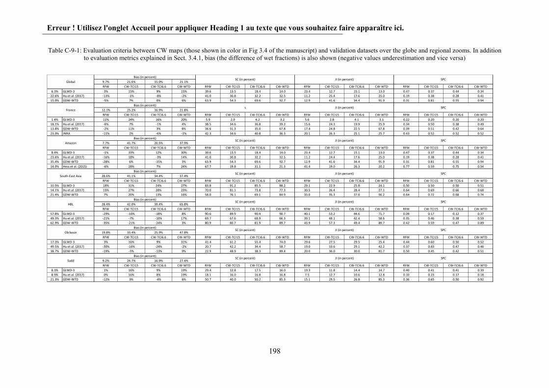
Erreur ! Utilisez l'onglet Accueil pour appliquer Heading 1 au texte que vous souhaitez faire apparaître ici.
198
Table C-9-1: Evaluation criteria between CW maps (those shown in color in Fig 3.4 of the manuscript) and validation datasets over the globe and regional zooms. In addition to evaluation metrics explained in Sect. 3.4.1, bias (the difference of wet fractions) is also shown (negative values underestimation and vice versa)
9.7% 21.6% 15.0% 21.1%RFW CW-TCI15 CW-TCI6.6 CW-WTD RFW CW-TCI15 CW-TCI6.6 CW-WTD RFW CW-TCI15 CW-TCI6.6 CW-WTD RFW CW-TCI15 CW-TCI6.6 CW-WTD
6.3% GLWD-3 3% 15% 9% 15% 39.6 13.5 18.4 14.0 23.4 12.7 15.1 13.0 0.47 0.37 0.44 0.3422.6% Hu et al. (2017) -13% -1% -8% -2% 41.0 30.8 32.2 32.5 11.2 25.4 17.6 25.0 0.19 0.38 0.28 0.4115.0% GDW-WTD -5% 7% 0% 6% 63.9 54.3 69.6 92.7 12.9 41.6 34.4 91.9 0.31 0.81 0.55 0.94
12.1% 25.2% 16.9% 21.8%RFW CW-TCI15 CW-TCI6.6 CW-WTD RFW CW-TCI15 CW-TCI6.6 CW-WTD RFW CW-TCI15 CW-TCI6.6 CW-WTD RFW CW-TCI15 CW-TCI6.6 CW-WTD
1.4% GLWD-3 11% 24% 16% 20% 5.9 2.9 4.2 3.2 5.6 2.8 4.1 3.1 0.22 0.20 0.20 0.2018.1% Hu et al. (2017) -6% 7% -1% 4% 38.5 34.6 36.8 39.2 15.6 24.3 19.9 25.9 0.34 0.50 0.38 0.4913.8% GDW-WTD -2% 11% 3% 8% 34.6 31.3 35.0 67.8 17.4 24.8 22.5 67.8 0.39 0.51 0.42 0.6423.0% INRA -11% 2% -6% -1% 42.3 34.6 40.8 36.3 20.1 26.3 25.1 25.7 0.43 0.52 0.52 0.52
7.7% 41.7% 20.5% 37.9%RFW CW-TCI15 CW-TCI6.6 CW-WTD RFW CW-TCI15 CW-TCI6.6 CW-WTD RFW CW-TCI15 CW-TCI6.6 CW-WTD RFW CW-TCI15 CW-TCI6.6 CW-WTD
8.4% GLWD-3 -1% 33% 12% 30% 39.6 13.5 18.4 14.0 23.4 12.7 15.1 13.0 0.47 0.37 0.44 0.3423.6% Hu et al. (2017) -16% 18% -3% 14% 41.0 30.8 32.2 32.5 11.2 24.4 17.6 25.0 0.19 0.38 0.28 0.4135.4% GDW-WTD -28% 6% -15% 3% 63.9 54.3 69.6 92.7 12.9 41.6 34.4 91.9 0.31 0.81 0.55 0.9414.0% Hess et al. (2015) -6% 28% 7% 24% 67.7 19.8 31.1 21.3 41.4 19.0 26.3 20.2 0.77 0.59 0.75 0.54
28.6% 41.1% 34.4% 37.4%RFW CW-TCI15 CW-TCI6.6 CW-WTD RFW CW-TCI15 CW-TCI6.6 CW-WTD RFW CW-TCI15 CW-TCI6.6 CW-WTD RFW CW-TCI15 CW-TCI6.6 CW-WTD
10.5% GLWD-3 18% 31% 24% 27% 83.8 91.2 85.5 88.2 29.1 22.9 25.8 24.1 0.50 0.50 0.50 0.5114.1% Hu et al. (2017) 15% 27% 20% 23% 70.0 81.1 73.8 77.3 30.5 26.4 28.4 27.1 0.64 0.69 0.66 0.6821.4% GDW-WTD 7% 20% 13% 16% 58.0 76.1 69.1 84.9 33.0 35.3 37.0 56.2 0.64 0.72 0.68 0.74
28.4% 42.0% 39.4% 65.8%RFW CW-TCI15 CW-TCI6.6 CW-WTD RFW CW-TCI15 CW-TCI6.6 CW-WTD RFW CW-TCI15 CW-TCI6.6 CW-WTD RFW CW-TCI15 CW-TCI6.6 CW-WTD
57.8% GLWD-3 -29% -16% -18% 8% 90.6 89.9 90.4 90.7 40.1 53.2 44.6 71.7 0.09 0.17 0.12 0.3749.3% Hu et al. (2017) -21% -7% -10% 17% 69.7 67.6 68.9 66.3 39.1 48.1 42.4 58.6 0.35 0.46 0.38 0.5962.9% GDW-WTD -35% -21% -24% 3% 80.9 80.7 81.9 89.7 43.9 57.3 49.4 89.7 0.42 0.59 0.47 0.89
19.8% 33.4% 25.9% 47.8%RFW CW-TCI15 CW-TCI6.6 CW-WTD RFW CW-TCI15 CW-TCI6.6 CW-WTD RFW CW-TCI15 CW-TCI6.6 CW-WTD RFW CW-TCI15 CW-TCI6.6 CW-WTD
17.3% GLWD-3 3% 16% 9% 31% 41.4 61.2 55.4 74.0 29.6 27.5 29.5 25.4 0.44 0.60 0.50 0.5249.5% Hu et al. (2017) -30% -16% -24% -2% 20.7 42.2 34.4 58.7 19.0 33.6 29.1 42.2 0.37 0.83 0.47 0.4638.7% GDW-WTD -19% -5% -13% 9% 22.9 48.9 38.3 89.4 20.0 36.0 30.0 81.7 0.50 0.45 0.42 0.51
9.2% 24.7% 16.9% 27.4%RFW CW-TCI15 CW-TCI6.6 CW-WTD RFW CW-TCI15 CW-TCI6.6 CW-WTD RFW CW-TCI15 CW-TCI6.6 CW-WTD RFW CW-TCI15 CW-TCI6.6 CW-WTD
8.3% GLWD-3 1% 16% 9% 19% 29.4 12.8 17.5 16.0 19.3 11.8 14.4 14.7 0.40 0.41 0.41 0.398.9% Hu et al. (2017) 0% 16% 8% 19% 18.1 16.0 16.8 16.8 7.5 12.7 10.6 12.8 0.10 0.23 0.17 0.18
21.3% GDW-WTD -12% 3% -4% 6% 50.7 40.0 50.2 85.3 15.1 29.5 26.8 85.3 0.36 0.65 0.50 0.92
FranceBias (in percent)
s JI (in percent) SPC
SuddBias (in percent)
SC (in percent) JI (in percent) SPC
Ob basinBias (in percent)
SC (in percent) JI (in percent) SPC
HBLBias (in percent)
SC (in percent) JI (in percent) SPC
South-East AsiaBias (in percent)
SC (in percent) JI (in percent) SPC
AmazonBias (in percent)
SC (in percent) JI (in percent) SPC
GlobalBias (in percent)
SC (in percent) JI (in percent) SPC

Erreur ! Utilisez l'onglet Accueil pour appliquer Heading 1 au texte que vous souhaitez faire apparaître ici.
199
Table C-9-2: Correlation between the developed and reference datasets (wetland fractions in 3 arcmin grid-cells) over the France. The highest three values in each column are shown in bold format, and grey cells give the
values used in Fig. 3.4 Dataset name ESA-CCI GIEMS-D15
JRC surface water
RFW GLWD-3 GDW-WTD Hu et al. (2017)
MPHFM
GDW-TI15 0.07 0.25 0.00 0.24 0.15 0.62 0.66 0.58
GDW-TCTrI15 -0.04 0.07 -0.05 0.06 -0.05 0.15 0.16 0.19
GDW-TCI15 0.04 0.23 -0.01 0.23 0.04 0.58 0.61 0.56
GDW-WTD 0.21 0.39 0.14 0.39 0.14 1.00 0.63 0.55
CW-TI6 0.31 0.90 0.25 0.89 0.20 0.45 0.42 0.52
CW-TCTrI6 0.31 0.90 0.25 0.89 0.20 0.39 0.35 0.49
CW-TCI6.6 0.31 0.89 0.25 0.87 0.20 0.42 0.38 0.52
CW-TI15 0.30 0.87 0.24 0.85 0.19 0.47 0.46 0.56
CW-TCTrI15 0.28 0.82 0.23 0.81 0.17 0.36 0.34 0.49
CW-TCI15 0.42 0.95 0.38 0.95 0.20 0.51 0.50 0.52
CW-WTD 0.42 0.93 0.37 0.92 0.20 0.64 0.49 0.52
ESA-CCI 1.00 0.43 0.80 0.43 0.31 0.21 0.16 0.30
GIEMS-D15 0.43 1.00 0.39 0.99 0.22 0.39 0.34 0.43
JRC surface water 0.80 0.39 1.00 0.39 0.16 0.14 0.09 0.22
RFW 0.43 0.99 0.39 1.00 0.22 0.39 0.34 0.43
GLWD-3 0.31 0.22 0.16 0.22 1.00 0.14 0.17 0.30
Hu et al. (2017) 0.16 0.34 0.09 0.34 0.17 0.63 1.00 0.58
MPHFM 0.30 0.43 0.22 0.43 0.30 0.55 0.58 1.00
Table C-9-3: Correlation between the developed and reference datasets (wetland fractions in 3 arcmin grid-cells) over the Amazon. The highest three values in each column are shown in bold format, and grey cells give the
values used in Fig. 3.4.
Dataset name ESA-CCI GIEMS-D15 JRC surface
water RFW GLWD-3 GDW-WTD
Hu et al. (2017)
Hess et al. (2015)
GDW-TI15 0.28 0.31 0.19 0.35 0.20 0.73 0.27 0.45
GDW-TCTrI15 -0.02 0.00 -0.03 0.01 -0.05 0.26 0.13 0.08
GDW-TCI15 0.22 0.19 0.12 0.25 0.21 0.81 0.37 0.35
GDW-WTD 0.29 0.27 0.17 0.31 0.25 1.00 0.40 0.40
CW-TI6 0.75 0.88 0.52 0.96 0.45 0.43 0.22 0.78
CW-TCTrI6 0.61 0.71 0.42 0.78 0.38 0.39 0.22 0.64
CW-TCI6.6 0.72 0.84 0.50 0.92 0.44 0.55 0.28 0.75
CW-TI15 0.72 0.85 0.50 0.93 0.45 0.53 0.26 0.78
CW-TCTrI15 0.34 0.39 0.23 0.43 0.20 0.36 0.21 0.37
CW-TCI15 0.48 0.53 0.31 0.59 0.37 0.81 0.38 0.59
CW-WTD 0.46 0.50 0.29 0.55 0.34 0.94 0.40 0.54
ESA-CCI 1.00 0.63 0.61 0.78 0.49 0.29 0.18 0.73
GIEMS-D15 0.63 1.00 0.56 0.92 0.42 0.27 0.17 0.67
JRC surface water 0.61 0.56 1.00 0.55 0.40 0.17 0.12 0.49
RFW 0.78 0.92 0.55 1.00 0.47 0.31 0.19 0.77
GLWD-3 0.49 0.42 0.40 0.47 1.00 0.25 0.19 0.47
Hu et al. (2017) 0.18 0.17 0.12 0.19 0.19 0.40 1.00 0.22
Hess et al. (2015) 0.73 0.67 0.49 0.77 0.47 0.40 0.22 1.00

Erreur ! Utilisez l'onglet Accueil pour appliquer Heading 1 au texte que vous souhaitez faire apparaître ici.
200
Table C-9-4: Correlation between the developed and reference datasets (wetland fractions in 3 arcmin grid-cells) over the SouthEast Asia. The highest three values in each column are shown in bold format, and grey cells give
the values used in Fig. 3.4.
Dataset name ESA-CCI GIEMS-D15 JRC surface
water RFW GLWD-3 GDW-WTD
Hu et al. (2017)
GDW-TI15 0.07 0.68 0.32 0.69 0.70 0.81 0.46
GDW-TCTrI15 -0.09 0.08 -0.06 0.07 0.04 0.15 -0.05
GDW-TCI15 0.13 0.72 0.36 0.71 0.73 0.81 0.53
GDW-WTD 0.16 0.64 0.42 0.64 0.72 1.00 0.49
CW-TI6 0.31 0.98 0.46 0.99 0.66 0.67 0.50
CW-TCTrI6 0.31 0.97 0.46 0.98 0.64 0.66 0.49
CW-TCI6.6 0.31 0.98 0.46 0.99 0.66 0.68 0.50
CW-TI15 0.30 0.98 0.45 0.99 0.67 0.68 0.50
CW-TCTrI15 0.28 0.89 0.41 0.90 0.61 0.63 0.44
CW-TCI15 0.31 0.95 0.45 0.95 0.69 0.73 0.50
CW-WTD 0.32 0.96 0.46 0.97 0.68 0.74 0.51
ESA-CCI 1.00 0.29 0.56 0.32 0.23 0.16 0.30
GIEMS-D15 0.29 1.00 0.46 0.99 0.63 0.64 0.49
JRC surface water 0.56 0.46 1.00 0.47 0.45 0.42 0.48
RFW 0.32 0.99 0.47 1.00 0.64 0.64 0.50
GLWD-3 0.23 0.63 0.45 0.64 1.00 0.72 0.57
Hu et al. (2017) 0.30 0.49 0.48 0.50 0.57 0.49 1.00
Table C-9-5: Correlation between the developed and reference datasets (wetland fractions in 3 arcmin grid-cells) over the Hudson Bay lowlands. The highest three values in each column are shown in bold format, and grey cells
give the values used in Fig 3.4.
Dataset name ESA-CCI GIEMS-D15 JRC surface
water RFW GLWD-3 GDW-WTD
Hu et al. (2017)
GDW-TI15 0.29 -0.09 -0.29 0.28 0.41 0.72 0.49
GDW-TCTrI15 0.13 0.08 -0.12 0.20 0.27 0.40 0.28
GDW-TCI15 0.37 -0.16 -0.31 0.29 0.43 0.72 0.49
GDW-WTD 0.52 0.00 -0.04 0.42 0.46 1.00 0.57
CW-TI6 0.77 0.47 0.22 0.99 0.13 0.49 0.39
CW-TCTrI6 0.74 0.47 0.21 0.95 0.15 0.49 0.39
CW-TCI6.6 0.79 0.48 0.23 0.99 0.12 0.47 0.38
CW-TI15 0.77 0.45 0.18 0.97 0.17 0.57 0.45
CW-TCTrI15 0.63 0.37 0.16 0.81 0.22 0.57 0.43
CW-TCI15 0.77 0.46 0.20 0.96 0.17 0.59 0.46
CW-WTD 0.61 0.26 0.09 0.67 0.37 0.89 0.59
ESA-CCI 1.00 0.06 0.13 0.78 0.23 0.52 0.35
GIEMS-D15 0.06 1.00 0.40 0.52 -0.21 0.00 0.07
JRC surface water 0.13 0.40 1.00 0.24 -0.30 -0.04 -0.01
RFW 0.78 0.52 0.24 1.00 0.09 0.42 0.35
GLWD-3 0.23 -0.21 -0.30 0.09 1.00 0.46 0.28
Hu et al. (2017) 0.35 0.07 -0.01 0.35 0.28 0.59 1.00

Erreur ! Utilisez l'onglet Accueil pour appliquer Heading 1 au texte que vous souhaitez faire apparaître ici.
201
Table C-9-6: Correlation between the developed and reference datasets (wetland fractions in 3 arcmin grid-cells) over the Ob river basin. The highest three values in each column are shown in bold format, and grey cells give
the values used in Fig 3.4.
Dataset name ESA-CCI GIEMS-D15 JRC surface
water RFW GLWD-3 GDW-WTD
Hu et al. (2017)
GDW-TI15 0.26 0.29 0.15 0.33 0.21 0.44 0.55
GDW-TCTrI15 0.12 0.11 0.10 0.16 0.13 0.11 0.20
GDW-TCI15 0.53 0.42 0.19 0.58 0.41 0.53 0.58
GDW-WTD 0.39 0.18 -0.07 0.37 0.33 1.00 0.55
CW-TI6 0.88 0.73 0.25 0.96 0.49 0.44 0.49
CW-TCTrI6 0.61 0.51 0.21 0.68 0.38 0.35 0.45
CW-TCI6.6 0.89 0.74 0.26 0.97 0.50 0.42 0.47
CW-TI15 0.85 0.70 0.22 0.94 0.49 0.48 0.54
CW-TCTrI15 0.50 0.39 0.10 0.55 0.33 0.31 0.37
CW-TCI15 0.86 0.69 0.22 0.97 0.51 0.46 0.52
CW-WTD 0.66 0.49 0.08 0.71 0.45 0.83 0.60
ESA-CCI 1.00 0.51 0.26 0.88 0.54 0.39 0.42
GIEMS-D15 0.51 1.00 0.32 0.73 0.26 0.18 0.31
JRC surface water 0.26 0.32 1.00 0.27 0.12 -0.07 0.21
RFW 0.88 0.73 0.27 1.00 0.50 0.37 0.44
GLWD-3 0.54 0.26 0.12 0.50 1.00 0.33 0.31
Hu et al. (2017) 0.42 0.31 0.21 0.44 0.31 0.55 1.00
Table C-9-7: Correlation between the developed and reference datasets (wetland fractions in 3 arcmin grid-cells) over the Sudd. The highest three values in each column are shown in bold format, and grey cells give the values
used in Fig 3.4.
Dataset name ESA-CCI GIEMS-D15 JRC surface
water RFW GLWD-3 GDW-WTD
Hu et al. (2017)
GDW-TI15 0.30 0.27 0.09 0.37 0.25 0.67 0.08
GDW-TCTrI15 -0.08 -0.04 -0.02 -0.07 -0.05 0.04 -0.04
GDW-TCI15 0.41 0.14 0.02 0.35 0.30 0.73 0.27
GDW-WTD 0.34 0.24 0.05 0.36 0.31 1.00 0.18
CW-TI6 0.79 0.72 0.28 0.95 0.40 0.51 0.11
CW-TCTrI6 0.80 0.74 0.29 0.96 0.39 0.38 0.10
CW-TCI6.6 0.80 0.71 0.28 0.95 0.41 0.50 0.17
CW-TI15 0.70 0.64 0.25 0.85 0.40 0.61 0.11
CW-TCTrI15 0.75 0.69 0.27 0.90 0.35 0.36 0.08
CW-TCI15 0.71 0.60 0.22 0.83 0.41 0.65 0.23
CW-WTD 0.55 0.48 0.17 0.66 0.39 0.92 0.18
ESA-CCI 1.00 0.35 0.20 0.83 0.42 0.34 0.12
GIEMS-D15 0.35 1.00 0.28 0.77 0.27 0.24 0.04
JRC surface water 0.20 0.28 1.00 0.30 0.18 0.05 -0.01
RFW 0.83 0.77 0.30 1.00 0.40 0.36 0.10
GLWD-3 0.42 0.27 0.18 0.40 1.00 0.31 0.13
Hu et al. (2017) 0.12 0.04 -0.01 0.10 0.13 0.18 1.00

Tootchi Ardalan – Thèse de doctorat - 2019
Résumé : Les zones humides jouent un rôle important dans le fonctionnement du système Terre aussi bien à l’échelle locale via un effet tampon sur les crues et épurateur de l’eau (dénitrification) que régionalement, du fait de leurs interactions avec l’atmosphère et de leur contribution majeure aux émissions de méthane. Leur représentation dans les modèles climatiques planétaires requiert une connaissance approfondie à la fois de leur distribution géographique et de leur hydrologie. Il y a un vaste désaccord sur l’estimation de l’étendue globale des zones humides, comprise entre 3% et 21% de la surface terrestre continentale, selon les méthodes employées. Ces contradictions s’expliquent par une représentation incomplète par les modèles hydrogéologiques des zones régulièrement inondées identifiées par l’imagerie satellitaire, qui peine en revanche à détecter les zones humides alimentées par les eaux souterraines. Peu visibles, elles sont également sous-estimées par la plupart des inventaires. La première étape de la thèse s’est donc focalisée sur la construction d’une carte mondiale des zones humides visant à concilier ces différences, par la distinction de ces deux types de zones humides, obtenus par combinaison des méthodes d’imagerie des eaux de surface et de modélisation des eaux souterraines. La proportion de zones humides à la surface du globe (21%) se situe dans la fourchette haute des estimations précédentes et concorde avec de nombreuses études régionales récentes, notamment en France et aux Etats-Unis. Dans une seconde étape, cette carte a servi d’entrée à une nouvelle version du modèle ORCHIDEE, qui décrit les surfaces continentales dans le modèle de climat de l’IPSL. La carte permet de distinguer dans chaque maille du modèle une fraction humide qui correspond aux fonds de vallée et reçoit les écoulements de la fraction haute, ce qui y rend possible le développement d’une nappe proche de la surface dont la profondeur répond au climat. Cette nouvelle version, dite ORCHIDEE-WET, a été testée dans le bassin de la Seine par comparaison à des observations de débit, d’évapotranspiration et de profondeur de nappe et afin de mieux comprendre l’effet des paramètres mal contraints tels que la profondeur du sol ou la formulation du flux nappe-rivière. Les effets principaux sont une augmentation de l’évaporation, une baisse des débits et un effet refroidissant, dont les conséquences sur le climat présent mais aussi futur sont une perspective importante à ce travail.
Mots clés : zones humides, modèle de surface, ORCHIDEE Abstract: Wetlands have significant functions in the Earth’s climate system both at local scales through their buffering effect on floods and water purification (denitrification) and also at a larger scale with their feedbacks to the atmosphere and its role in methane emission. To include wetlands in climate models globally, both their geographic distribution and hydrology should be known. There is a massive inconsistency among wetland mapping methods and wetland extent estimates (from 3 to 21% of the land surface area), rooted in imagery disturbances, underestimation of the groundwater driven wetlands in inventories or imprecise representation of flooded zones in GW modellings. In the framework of this PhD project, first by developing a global wetland map through a multi-source data fusion method we provide a simple applied classification for wetlands hydrological roles. Wetlands’ global extent is estimated to be almost 24.3 106 km2 (including lakes). The core distinction between classes is the flooding conditions and the water source, either coming from surface streams or groundwater convergence. In the next step, we modelled the wetlands’ role on surface processes in ORCHIDEE land surface model which was the testing platform for this new hydrologic scheme at large scale. The basic assumption in the new version (ORCHIDEE-WET) in this sub-grid procedures is that the deep drainage from the uplands converges over lowland wet fraction in parallel to infiltration from precipitation. Simulations over the contemporary era under climate forcing shows that the water table goes deeper with increased potential wetland fraction. The water table is shallow enough to be considered actual wetland when the potential wetland fraction is less than 0.2 over the Seine River Basin. The evapotranspiration rate increases by almost 3% with ORCHIDEE-WET because of the increased soil moisture in the wetland soil column. Increased soil moisture in the wet fraction affects the soil surface temperature as well. The future applications of this PhD work can be to explicitly introduce the biogeochemical procedures in wetlands in a dynamic manner to study the feedback effects of wetlands on climate and the Carbon cycle.
Keywords: Wetland, Land surface model, ORCHIDEE
Copyright © 2022 FDOKUMEN