
Sorbonne Université Optical detection of magneto-acoustic ...
162
Sorbonne Université École doctorale 397: Physique et Chimie des Matériaux Thèse de DOCTORAT Spécialité Physique présentée par Piotr Kuszewski Pour obtenir le grade de Docteur de: Sorbonne Université Sujet de la thèse Optical detection of magneto-acoustic dynamics soutenue le 9 Novembre 2018 Devant le jury composé de: Rapporteur Olivier Klein CEA Rapporteur Thomas Pezeril Université du Maine Examinateur Sarah Benchabane Gaiffe FEMTO-ST Examinateur Karine Dumesnil Institut Jean Lamour Examinateur Massimiliano Marangolo Institut des NanoSciences de Paris Directeur de thèse Catherine Gourdon Institut des NanoSciences de Paris
-
Upload
khangminh22 -
Category
Documents
-
view
4 -
download
0
Transcript of Sorbonne Université Optical detection of magneto-acoustic ...
Sorbonne UniversitéÉcole doctorale 397: Physique et Chimie des Matériaux
Thèse de DOCTORAT
Spécialité Physique
présentée par
Piotr Kuszewski
Pour obtenir le grade de Docteur de: Sorbonne Université
Sujet de la thèse
Optical detection of magneto-acoustic dynamicssoutenue le 9 Novembre 2018
Devant le jury composé de:
Rapporteur Olivier Klein CEARapporteur Thomas Pezeril Université du MaineExaminateur Sarah Benchabane Gaiffe FEMTO-STExaminateur Karine Dumesnil Institut Jean LamourExaminateur Massimiliano Marangolo Institut des NanoSciences de ParisDirecteur de thèse Catherine Gourdon Institut des NanoSciences de Paris


Abstract
In the developing field of spin wave-based information technology, this work in-vestigates the possibility to use surface acoustic waves (SAW) to excite spin-wavesin ferromagnetic thin layers relying on the magnetoelastic coupling. This wouldprovide a non-inductive, efficient, and remote addressing of spin waves.In the first project we develop an experimental setup to generate electrically excitedSAWs phase-locked to probe laser pulses. The magnetization dynamics is detectedby an optical bridge using magneto-optical effects (Kerr and Voigt). We investigatethe resonant magneto-elastic coupling in a thin film of the ferromagnetic semicon-ductor (Ga,Mn)As. To reach resonant coupling, the spin-wave frequency is scannedacross the SAW frequency using a magnetic field. We disentangle the photoelasticcontribution from the magneto-optical one, from which we obtain the amplitude ofmagnetization precession. We show that it is driven solely by the acoustic wave. Itsfield dependence is shown to agree well with theoretical calculations. Its amplituderesonates at the same field as the resonant attenuation of the acoustic wave, clearlyevidencing the magnetoacoustic resonance with high sensitivity. The influence oftemperature, SAW frequency and power on the coupling efficiency are studied.In the second project we use SAWs thermoelastically excited by a tightly focusedlaser beam on ferromagnetic metals (Ni, FeGa, Co) on a transparent substrate (glass,sapphire). Spatio-temporal maps of the surface displacement and magneto-opticalsignal are obtained. A high-frequency shift of the frequency spectrum of the lattergives a hint for spin-wave excitation by SAWs.

Résumé
Ce travail se situe dans le contexte de l’utilisation des ondes de spin comme vecteurd’information. Il explore la possibilité d’exciter l’aimantation dans de fines couchesferromagnétiques grâce au couplage magnéto-élastique. Cela permettrait un adres-sage non-inductif, efficace, et distant des ondes de spin.Dans un premier volet, nous avons développé un dispositif expérimental générantdes ondes acoustiques de surface (ODS) électriquement, verrouillées en phase à desimpulsions de laser sonde. La dynamique d’aimantation est détectée grâce auxeffets magnéto-optiques (Kerr et Voigt). Nous étudions le couplage magnétoélas-tique résonant dans une couche mince du semiconducteur magnétique (Ga,Mn)As.Afin d’atteindre la résonance, la fréquence des ondes de spin est ajustée à celle desODS par un champ magnétique. Nous isolons les contributions photo-élastique etmagnéto-optique du signal, pour quantifier l’amplitude de la précession d’aimantation.Nous montrons que la précession observée est exclusivement déclenchée par l’ODS.La variation en champ de son amplitude correspond très bien à celle calculée, et elleest maximum au champ pour laquelle l’absorption de l’ODS est maximale, démon-trant clairement la résonance magnétoacoustique. L’influence de la fréquence et dela puissance de l’ODS, ainsi que de la température sur l’efficacité du couplage estégalement explorée.Dans un deuxième volet, nous avons excité des ODS par effet thermoélastique grâceà un faisceau laser focalisé, et cela sur des couches magnétiques métalliques cettefois-ci (Ni, FeGa, Co), déposées sur un substrat transparent (verre, sapphire). Descartes spatio-temporelles du déplacement de la surface et du signal magnéto-optiqueont été obtenues. Un décalage du spectre magnéto-optique vers les hautes fréquencessemble indiquer une excitation des ondes de spin par les ODS.


Contents
Introduction 1
1. Magnetization dynamics 71.1. Landau-Lifshitz-Gilbert equation . . . . . . . . . . . . . . . . . . . . 71.2. Free energy density of the ferromagnetic material . . . . . . . . . . . 8
1.2.1. Zeeman energy . . . . . . . . . . . . . . . . . . . . . . . . . . 81.2.2. Exchange energy . . . . . . . . . . . . . . . . . . . . . . . . . 91.2.3. Demagnetizing energy . . . . . . . . . . . . . . . . . . . . . . 91.2.4. Magnetocrystalline anisotropy energy . . . . . . . . . . . . . . 101.2.5. Equilibrium orientation of the magnetization . . . . . . . . . . 11
1.3. Spin waves . . . . . . . . . . . . . . . . . . . . . . . . . . . . . . . . . 121.3.1. Types of spin waves . . . . . . . . . . . . . . . . . . . . . . . . 121.3.2. Excitation of spin waves . . . . . . . . . . . . . . . . . . . . . 15
2. Acoustic waves 192.1. Types of acoustic waves . . . . . . . . . . . . . . . . . . . . . . . . . 192.2. Elastic energy . . . . . . . . . . . . . . . . . . . . . . . . . . . . . . . 202.3. Wave equation . . . . . . . . . . . . . . . . . . . . . . . . . . . . . . . 222.4. Rayleigh waves . . . . . . . . . . . . . . . . . . . . . . . . . . . . . . 232.5. Excitation of acoustic waves . . . . . . . . . . . . . . . . . . . . . . . 27
2.5.1. Optical excitation technique . . . . . . . . . . . . . . . . . . . 272.5.2. Electrical excitation technique . . . . . . . . . . . . . . . . . . 29
3. Magneto-elastic dynamics 333.1. Magnetostriction . . . . . . . . . . . . . . . . . . . . . . . . . . . . . 333.2. Magneto-elastic energy . . . . . . . . . . . . . . . . . . . . . . . . . . 33
3.2.1. Contribution of magneto-elasticity to the magnetocrystallineanisotropy energy . . . . . . . . . . . . . . . . . . . . . . . . . 35
3.3. Effect of the magneto-elastic coupling on magnetization and straindynamics . . . . . . . . . . . . . . . . . . . . . . . . . . . . . . . . . 36
4. Static and dynamic control of the magnetization with strain: state ofthe art 394.1. Static strain . . . . . . . . . . . . . . . . . . . . . . . . . . . . . . . . 394.2. Dynamic strain . . . . . . . . . . . . . . . . . . . . . . . . . . . . . . 41
4.2.1. Non-resonant interaction . . . . . . . . . . . . . . . . . . . . . 414.2.2. Resonant interaction . . . . . . . . . . . . . . . . . . . . . . . 42
i

Contents Contents
5. Experimental techniques 495.1. Magnetic characterization . . . . . . . . . . . . . . . . . . . . . . . . 50
5.1.1. Cavity FMR . . . . . . . . . . . . . . . . . . . . . . . . . . . . 505.1.2. Broadband FMR (BBFMR) . . . . . . . . . . . . . . . . . . . 515.1.3. Vibrating-sample magnetometer (VSM) . . . . . . . . . . . . . 53
5.2. Time and frequency domain detection of spin waves . . . . . . . . . . 535.2.1. Faraday effect . . . . . . . . . . . . . . . . . . . . . . . . . . . 535.2.2. Magneto-optical Kerr effect . . . . . . . . . . . . . . . . . . . 575.2.3. Voigt effect . . . . . . . . . . . . . . . . . . . . . . . . . . . . 585.2.4. Brillouin light scattering spectroscopy (BLSS) . . . . . . . . . 60
5.3. Detection of Surface acoustic waves - Photo-elastic effect . . . . . . . 625.4. Materials . . . . . . . . . . . . . . . . . . . . . . . . . . . . . . . . . 63
5.4.1. GaMnAs . . . . . . . . . . . . . . . . . . . . . . . . . . . . . 645.4.2. Ferromagnetic metals . . . . . . . . . . . . . . . . . . . . . . . 65
6. Spatial and dynamical control of magnetization with electrically excitedsurface acoustic waves 716.1. Phase synchronization . . . . . . . . . . . . . . . . . . . . . . . . . . 72
6.1.1. Experimental set-up . . . . . . . . . . . . . . . . . . . . . . . 736.1.2. Jitter measurement . . . . . . . . . . . . . . . . . . . . . . . . 746.1.3. Lock-in detection of the optical signal . . . . . . . . . . . . . . 766.1.4. IDT design . . . . . . . . . . . . . . . . . . . . . . . . . . . . 776.1.5. Phase between the optical and electrical signal . . . . . . . . . 81
6.2. Detection of the magneto-acoustic signal . . . . . . . . . . . . . . . . 826.2.1. Burst shape . . . . . . . . . . . . . . . . . . . . . . . . . . . . 85
6.3. Polarization dependence studies . . . . . . . . . . . . . . . . . . . . . 866.3.1. Methodology . . . . . . . . . . . . . . . . . . . . . . . . . . . 866.3.2. Field dependence . . . . . . . . . . . . . . . . . . . . . . . . . 876.3.3. The magnetization precession excitation efficiency versus SAW
frequency . . . . . . . . . . . . . . . . . . . . . . . . . . . . . 896.3.4. Phase of the TRPR signal . . . . . . . . . . . . . . . . . . . . 906.3.5. Temperature dependence . . . . . . . . . . . . . . . . . . . . . 916.3.6. Power dependence . . . . . . . . . . . . . . . . . . . . . . . . 936.3.7. Back-action of the magnetization precession on SAW - SAWFMR 946.3.8. Spatial mapping of the magnetic and acoustic waves . . . . . . 97
6.4. Perspectives . . . . . . . . . . . . . . . . . . . . . . . . . . . . . . . . 101
7. Spatial and dynamical control of magnetization with optically excitedsurface acoustic waves 1037.1. Introduction . . . . . . . . . . . . . . . . . . . . . . . . . . . . . . . . 1037.2. Set-up and samples . . . . . . . . . . . . . . . . . . . . . . . . . . . . 104
7.2.1. Set-up . . . . . . . . . . . . . . . . . . . . . . . . . . . . . . . 1047.2.2. Measurement procedure . . . . . . . . . . . . . . . . . . . . . 1067.2.3. Expected polarization rotation map symmetry . . . . . . . . . 108
ii

Contents
7.2.4. Samples (guidelines) . . . . . . . . . . . . . . . . . . . . . . . 1107.3. Results . . . . . . . . . . . . . . . . . . . . . . . . . . . . . . . . . . . 111
7.3.1. FeGa in zero-field: high precession frequency . . . . . . . . . . 1117.3.2. Nickel in zero-field: low precession frequency . . . . . . . . . . 1147.3.3. FeGa under magnetic field . . . . . . . . . . . . . . . . . . . . 1217.3.4. Comparison of dispersion maps for FeGa, Co and Ni . . . . . 1267.3.5. Confrontation with the non-magnetic sample . . . . . . . . . . 129
7.4. Conclusions and perspectives . . . . . . . . . . . . . . . . . . . . . . . 130
Conclusions and perspectives 131
A. Expression for the polarization rotation detected with Lock-in 133
Bibliography 137
iii


IntroductionThe first commercially available computer with a magnetic hard drive disk was theIBM 305 RAMAC (Random Access Memory Accounting) developed in 1956 [1]. Itssize was extremely large, only the disk storage unit covered the space equivalent toone taken by three refrigerators (Fig. 0.1 (a)). The monthly cost of the data storagewas $ 3 200 which is over $ 28 000 nowadays and $ 7 500 per MB. Nevertheless,over 1000 of these computers were built in 4 years, because of their high capacity,3.75 MB (5 million alphanumeric characters), and a fast access time to any bit(average 0.6 s). This changed once and for all the perception of magnetism as atechnologically attractive solution for data computing.
Figure 0.1.: (a) Picture of the IBM 350 data storage unit taken at the AmsterdamSchiphol airport in 1957 [2]. In this model, data was saved on one of 50 spinningAluminium discs coated with Iron oxide. (b) The general concept of the HDD:the recording head is used to write and read the bits in a thin ferromagnetic film.It is mounted on a movable arm which moves across the rotating disc. The redand blue colors indicate opposite directions of magnetization. (c) The racetrackmemory concept proposed in 2008 by Stuart Parkin [3].
The magnetic recording revolution has been lasting for the last 60 years and allowedus to forget for instance about punched cards. The capacity of a magnetic hard
1

disk drive (HDD) reached above 10 TB in 2018 with an areal density of around1.4 Tbit/in2. However, this is a 2D technology which is very close to the physicallimit, therefore to increase the storage density, the world demands new solutions.One of the concepts of the 3D data storage is the racetrack memory, where thedata will be saved in domains separated by domain walls in thin magnetic wiresarranged in a high density array (Fig. 0.10.1 (c)) [3]. The domain walls couldbe moved along the wire with a spin polarized current to shift the bits (magneticdomains) to read and write sections. This device will not require any mechanicallymovable parts. Thus, the read and write time can be lowered by million timescompared to the standard HDD discs. Of course, magnetism is not only used fordata storage but also in data transport [4, 5], logic gates[6] and in the widest sense,in signal processing[7] including non-boolean, wave-based computing [8, 9] (Fig.0.2). Magnetization dynamics, can be described in terms of spin waves, where thespin excitations can propagate in a coherent way. The quanta of magnetizationdynamics are called magnons in analogy with phonons or photons. Similarly tophotonics, magnonics aim to design new architectures to built new functionalitiesusing magnons.
2

Figure 0.2.: A few chosen experiments that illustrate the possible usage of magnon-ics in signal processing. (a) Image of a spin wave intensity propagating in a ge-ometrically curved YIG waveguide [5]. (b) One example of a non boolean signaldevice: schematics of the spin wave based spectrum analyzer. Spin waves areexcited with the antenna and then they are diffracted on a curved diffractiongrating. If the spin waves are generated with a current carring multiple frequen-cies, the diffrent wavelengths will be focused at different places on the right side[10]. (c) Scheme of the magnonic transistor, based on a magnonic crystal. Themagnons injected in the source propagate to the drain in the case when there isno gate-magnons. Gate-magnons are at the frequency of the magnonic crystalbandgap, thus they do not propagate to the drain. Therefore, the high densityof the gate-magnons scatters nonlinearly the source magnons and lowers the onestransmitted to the drain [11]. (d) Picture of the magnonic majority gate realizedin 2017 [12]. The spin waves injected to the three inputs interfere with each otherand the information is decoded at the output from the phase of the signal.
Indeed, magnonics and photonics are often linked and where they come together itmakes the project far-reaching. The power of magnonics lies in its elemental prop-erties, such as the µm-nm spin wave wavelength (GHz-THz frequency regime) andthe absence of Joule heating: in magnon transport there is no charge transfer, onlyangular momentum transfer. Moreover, magnon properties can be tuned in a varietyof ways e.g. by changing the magnetic material and its geometry, temperature, mag-
3

netic field and direction of the field [8]. So far, the most common excitation of spinwaves was an inductive antenna. This is a solution, that is easy to implement andwhich can be also used to detect the spin waves. However, antenna excitation is theweakest point of spin wave-based computing systems due to its low energy efficiencyand limitation to long wavelengths because of the impedance mismatch (the widthof the antenna needs to be smaller than the spin wave wavelength) [9]. Moreover inmost ferromagnetic materials spin waves are damped over short distances (tens ofµm). Some of these limitations can be overcome by using magneto-elastic coupling.This field has witnessed a renewed interest in recent years with the extensive workof a few groups that brought very promising achievements e.g. acoustically drivenferromagnetic resonance[13, 14] and switching [15, 16] or acoustically assisted, effi-cient domain wall motion for the above-mentioned racetrack memories [17, 18]. Itis expected that magneto-acoustic wave could propagate on larger distances thanspin waves. Furthermore, using the low damping property of acoustic waves meansthat they can be excited remotely in the desired point on the magnetostrictive ma-terial. The research field that combines magnonics and strain (dynamic or static)has recently been referred to as straintronics[19].Our research group started working with straintronics in 2010 by using optically ex-cited strain pulses for the magnetization precession excitation in thin GaMnAs films[20]. These picosecond strain pulses were excited on the rear face of the sample andtraveled through the substrate to arrive to the magnetic layer. This excitation wasfound not to be very efficient due to the weak coupling between the excited straincomponents and the magnetization, and the frequency and the wavevector mismatchbetween strain waves and spin waves. That is why in 2013 the group headed towardselectrically excited surface acoustic waves. This type of acoustic waves, as they arenamed, propagate at the surface of the sample, where they are weakly damped,and their amplitude decreases exponentially in the depth of the material. It makesthem ideal candidates for working with thin magnetic films. Heretofore, the grouphas reported magnetization switching and ferromagnetic resonance driven by surfaceacoustic waves [21, 14, 16]. In these experiments, changes in static magnetizationwere probed optically by static Kerr microscopy and magnetization dynamics wasdetected indirectly as the changes of surface acoustic wave amplitude and phase.A direct evidence of strain-wave induced magnetization dynamics was still missing.In 2015, the group decided to launch two new projects that became the subject ofmy PhD work: in the first one, surface acoustic waves were excited electrically andthe dynamic magnetization was detected optically which had never been reportedbefore (Chapter 6). In the second project surface acoustic waves were excited opti-cally and magnetization/strain dynamics were also detected optically (Chapter 7).In between 2015 and 2018 many articles came out concerning similar physics. Theyhave explored different geometries that will be detailed in Chapter 4. For the firstproject we worked with ferromagnetic semiconductor GaMnAs, a low Curie temper-ature ferromagnet but with adjustable magnetic properties. For a second one weturned to ferromagnetic metals with Curie temperature above room temperature.
4

We believe that the results presented in this work may contribute to improve thealready existing concepts of magnon based signal processing or help to develop newones.The manuscript is organized as follows. In Chapter 1 the theory on magnetizationdynamics will be introduced. We will describe the main components of the freeenergy of the ferromagnetic thin samples. Also the full energy expression for GaM-nAs will be given. Later in the same chapter the concept of spin waves is discussedand the most common excitation techniques are shown, including magneto-acousticcoupling, to which this work is devoted. In Chapter 2 you will find the description ofacoustic waves with a strong emphasis on surface acoustic waves. In Chapter 3 thetheory of magneto-acoustics is shown. Chapter 4 presents the literature review ontopics related to this thesis. The following chapters are dedicated to experiments.Thus, Chapter 5 recalls the experimental techniques used and shows the magneticcharacteristics of the samples investigated. Chapter 6 contains the results of thefirst project, where surface acoustic waves were excited electrically and magneti-zation dynamics was detected optically. In the few first pages of this chapter, theexperimental set-up that was developed is extensively described. Chapter 7 containsthe experimental results for the second project, made in collaboration with LaurentBelliard. In this chapter many 2D maps of magneto-acoustic signal are shown.
5


1. Magnetization dynamics
Table of content
1.1 Landau-Lifshitz-Gilbert equation1.2 Free energy density of the ferromagnetic material
1.2.1 Zeeman energy1.2.2 Exchange energy1.2.3 Demagnetizing energy1.2.4 Magnetocrystalline anisotropy energy1.2.5 Equilibrium orientation of the magnetization
1.3 Spin waves1.3.1 Types of spin waves1.3.2 Excitation of spin waves
1.1. Landau-Lifshitz-Gilbert equation
The primary formulation of magnetization precessional motion was given in 1935 byL.D. Landau and E.M. Lifshitz [22, 23]. This is the elemental equation describing theundamped precessional motion of magnetic moments around the effective field. Theeffective field is the sum of all magnetic fields and it is defined as the derivative of thetotal energy of the ferromagnetic system with respect to ~m, described in the nextparagraph. Surely, this is not the real situation, since the magnetization would keepprecessing around the equilibrium position ( ~m ‖ ~Heff ) without energy dissipation,and it would never align with it. That is why in 1955 T.L. Gilbert proposed to add adamping part to the equation [24]. He introduced a small torque field which bringsthe magnetization towards the effective field. The spiral-like precessional motion, isunderstood as the nonlinear spin relaxation:
∂ ~m
∂t= −γµ0 ~m× ~Heff + α ~m× ∂ ~m
∂t(1.1)
where γ is the gyromagnetic factor (γ > 0), µ0 is the permeability of vacuum, ~m isthe magnetization unit vector ( ~M/Ms), α is the dimensionless damping factor.
7

Chapter 1 Magnetization dynamics
Figure 1.1.: The trajectory of the magnetization described by the Landau-Lifshitz-Gilbert equation.
1.2. Free energy density of the ferromagneticmaterial
The free energy density ( fV) of the ferromagnetic system contains the following
contributions: Zeeman energy, exchange energy, demagnetization energy, magne-tocrystaline anisotropy energy:
fV olume = f
V= fZeem + fExch + fDem + fMCA (1.2)
The relation between the effective field and the energy is given by the followingequation:
~Heff = − 1µ0~∇mf (1.3)
1.2.1. Zeeman energy
The Zeeman energy arises from the interaction of the magnetic moments with theexternal magnetic field. This energy is minimized when the magnetization lies alongthe direction of the magnetic field.
fZeem = −µ0(~M · ~H
)(1.4)
8

1.2 Free energy density of the ferromagnetic material
1.2.2. Exchange energy
The long range order in the ferromagnetic materials originates from the exchangeinteraction between the electron spins. The theory of exchange interaction is basedon the Pauli exclusion principle and Coulomb electrostatic forces. Because of thePauli principle, parallel electron spins are spread away and this lowers the Coulombinteraction between them. The energy difference between the parallel and antipar-allel spins is the exchange energy [25]. In quantum mechanics this can be writtenas the Heisenberg Hamiltonian:
H = −∑i, j
Jij ~Si · ~Sj (1.5)
Si and Sj are the i and j spins and Jij is the exchange integral between them. Forferromagnets Jij is positive. For the continuous ferromagnetic medium the sum canbe replaced by an integral. Keeping only nearest neighbors interaction (J), Equation1.5 leads to an energy density [26, 27]:
fExch = AExch |∇ ~m |2, (1.6)
where AExch for cubic crystals is defined as AExch = 2JS2
aand a is the distance
between the closest spins. In (Ga,Mn)As, Manganese spins are too dilute to interactdirectly. Instead, they interact via the spins of the delocalized holes. Hence, inGaMnAs AExch =0.4 pJ/m [28] is quite low compare to for example FeGa AExch =16pJ/m [29].
1.2.3. Demagnetizing energy
The demagnetizing energy arises from the demagnetizing field ~HDem and it isstrongly dependent on the shape of the ferromagnetic sample. The energy is de-fined as an integral over the sample shape:
fDem = 12µ0
∫sample
~M · ~HDemdV (1.7)
For a thin ferromagnetic film (thickness-d significantly smaller than the lateral di-mensions) it becomes [30]:
fV olumeDem = 12µ0M
2s cos2 θ (1.8)
9

Chapter 1 Magnetization dynamics
where θ is the angle with the normal to the film plane. The energy is minimized whenthe magnetization lies in-plane and this is the equilibrium position for most very thinmagnetic films (d < 1µm [31]). Moreover, the demagnetizing energy is proportionalto the square of the magnetization saturation, it means that for materials with a highMs value, a huge magnetic field will need to be applied to bring the magnetizationout of the sample plane. For instance metals have a very high Ms, the typical valuesare 1.7× 10⁶A/m for Fe, 1.4× 10⁶A/m for Co [27]. Therefore we will need around 2T to magnetize a sample out of the plane. However, this value is much smaller forferromagnetic semiconductors such as GaMnAs, the magnetization saturation forthis material is around 3.3× 10⁴A/m [32] and then the required field is 40 mT.
1.2.4. Magnetocrystalline anisotropy energy
In crystalline materials, the magnetization prefers to orient along certain crystallo-graphic axes. For these positions, the magnetocrystalline anisotropy (MCA) energyis minimized. In the literature, the axis with the lowest MCA energy for bulk ma-terials is named easy axis, while the axis for which the energy is maximal is calledhard axis. The MCA depends on the crystal symmetry, for instance the easy axes forbody-centered cubic Iron are <100>. While for face-centered cubic Nickel, <111>are the easy axes [33]. The origin of MCA lies in the spin-orbit interaction and theinteraction with the neighbor’s atoms via the crystal field. Strongly coupled nonspherically shaped orbitals will favor certain orientations of the spins. This appliesto transition metals, while for GaMnAs the mechanism is different since the orbitalangular momentum for the d5 Mn electron configuration is zero (L=0). The inter-actions between the localized spins are mediated by the holes, which carry non zerototal angular momentum, J 6=0 (J=L+S) [34]. It is thus the valence band structure,in which holes reside, that will govern the anisotropy.
1.2.4.1. Phenomenological description of the magnetocrystalline energy
The most general formula of the MCA energy is given by the expansion series of the~m components [27]. For cubic systems with crystallographic axes oriented parallelto the xyz coordinate system, the MCA energy can be written as follows:
fMCA = K1(m2xm
2y +m2
ym2z +m2
xm2z) +K2(m2
xm2ym
2z) + ... (1.9)
K1 andK2 are the anisotropy constants (higher orders are often negligible). In manytextbooks, you can find the above equation expressed by the directional cosines. Herewe used a different notation for the reader’s comfort. Hence the energy consists onlyof theKi and square of ~m , the whole function is even. It means that we will consideronly the orientation and not the direction of the easy and hard axis. This is causedby the crystal symmetry.
10

1.2 Free energy density of the ferromagnetic material
We will introduce now the MCA anisotropy for (Ga,Mn)As zinc-blende structurewith a tetragonal distortion:
fGaMnAsMCA = −K2⊥m
2z −
K4‖
2(m4x +m4
y
)− K4⊥
2 m4z −
K2‖
2 (mx −my)2 (1.10)
Equation 1.10 can be obtained from 1.9 by using the relationship for cubic crystals:
1 =(m2x +m2
y +m2z
)2= m4
x +m4y +m4
z + 2(m2xm
2y +m2
ym2z +m2
xm2z
)(1.11)
Therefore, the first term of equation 1.9 can be rewritten as:
fMCA = K1
2 (m4x +m4
y +m4z) (1.12)
provided that the constant term is dropped. Hence you can notice that for (Ga,Mn)Aswith no tetragonal distortion:
K4‖ = K4⊥ = K1
2 (1.13)
1.2.5. Equilibrium orientation of the magnetization
Once the most general static energy components were defined, the equilibrium po-sition of the magnetization can be found. For the simplicity of the calculations wewill work in the polar coordinate system:
Figure 1.2.: Location of magnetization in polar coordinates system.
11
Chapter 1 Magnetization dynamics
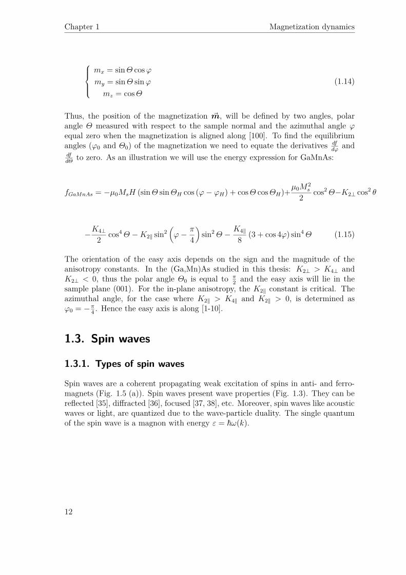
mx = sinΘ cosϕmy = sinΘ sinϕmz = cosΘ
(1.14)
Thus, the position of the magnetization ~m, will be defined by two angles, polarangle Θ measured with respect to the sample normal and the azimuthal angle ϕequal zero when the magnetization is aligned along [100]. To find the equilibriumangles (ϕ0 and Θ0) of the magnetization we need to equate the derivatives df
dϕand
dfdΘ
to zero. As an illustration we will use the energy expression for GaMnAs:
fGaMnAs = −µ0MsH (sinΘ sinΘH cos (ϕ− ϕH) + cosΘ cosΘH)+µ0M2s
2 cos2 Θ−K2⊥ cos2 θ
−K4⊥
2 cos4 Θ −K2‖ sin2(ϕ− π
4
)sin2 Θ −
K4‖
8 (3 + cos 4ϕ) sin4 Θ (1.15)
The orientation of the easy axis depends on the sign and the magnitude of theanisotropy constants. In the (Ga,Mn)As studied in this thesis: K2⊥ > K4⊥ andK2⊥ < 0, thus the polar angle Θ0 is equal to π
2 and the easy axis will lie in thesample plane (001). For the in-plane anisotropy, the K2‖ constant is critical. Theazimuthal angle, for the case where K2‖ > K4‖ and K2‖ > 0, is determined asϕ0 = −π
4 . Hence the easy axis is along [1-10].
1.3. Spin waves
1.3.1. Types of spin waves
Spin waves are a coherent propagating weak excitation of spins in anti- and ferro-magnets (Fig. 1.5 (a)). Spin waves present wave properties (Fig. 1.3). They can bereflected [35], diffracted [36], focused [37, 38], etc. Moreover, spin waves like acousticwaves or light, are quantized due to the wave-particle duality. The single quantumof the spin wave is a magnon with energy ε = ~ω(k).
12

1.3 Spin waves
Figure 1.3.: Schemes of experimental concepts for spin waves a) reflection [35] andb) diffraction[36]. c) Map of the spin wave intensity in a Permalloy film[38].
Depending on the wavevector k value and orientation with respect to ~M and ~H ,different interactions will play a role in the spin wave propagation and differentmodes will be distinguished. Spin wave modes are described by the dispersion rela-tion ω(k), which is commonly found by solving the LLG equation. Thus, equation1.1 in spherical coordinates in the case of a small angle of precession is given as [21]:
δϕ̇ = γsinΘ0
(fΘϕδϕ+ fΘΘδΘ) + αsinΘ0
δΘ̇
−δΘ̇ = γsinΘ0
(fϕϕδϕ+ fϕΘδΘ) + αδϕ̇ sinΘ0(1.16)
where fln = ∂2f∂l∂n
for l, n = ϕ or Θ and the dot denotes the derivative with respectto time l̇ = ∂l
∂t. Solving the LLG equations we are looking for the solution in k, thus
~m = ~m0 + ~δmei(~k~r−ωt) is the plane wave. The wavevector puts different weight onthe components of the free energy of the ferromagnet f : exchange energy (Section1.2.2) and demagnetizing energy (Section 1.2.3), since the short range (exchange en-ergy) and long range (demagnetizing energy) interactions have different dependenceon k. Consequently, we can distinguish three main regions defined by k (Fig. 1.4)[39]:
• k <105 cm-1: region dominated by the long range (long wavelength: λ >60 µm) dipole-dipole interactions. Those interactions are described by thedemagnetizing energy. The spin waves belonging to this group are calledmagnetostatic spin waves. Depending on the ~m orientation with respect tothe external magnetic field and the sample planes, different spin waves can bediscriminated [40].
• k >106 cm-1: spin waves in this range are dominated by exchange interactions,the wavelength of those spin waves is short (λ < 6 µm).
• 105 cm-1< k <106 cm-1: intermediate region were the two interactions have asimilar influence: they are called dipole-exchange spin waves.
13

Chapter 1 Magnetization dynamics
Figure 1.4.: Illustration of spin wave dispersion with two main regions: one dom-inated by the dipolar interactions and that other by the exchange interactions.From the slope of the presented curve the velocity of the propagating spin wavescan be obtained. When the slope is 0, those are stationary (non propagating) spinwaves. [41]
Moreover, the wavevector for a sample with finite lateral dimensions will be quan-tized due to the boundary conditions e.g. for themagnetic wall boundary condition,magnetization is pinned at the lateral edges. Thus the wavevector can only be inte-gral multiples of the spin waves halfwavelength [42]. However, in this thesis ~k was de-fined by the wavevector of SAWs, which was rather small: kSAW ≤ 2π
4.7µm∼= 1.3×10⁴
cm-1. The energy characteristic for this range of ~k is flat and can be read asω(k = kSAW ) ' ω(k = 0) (Fig. 3.2). The wavelength of spin waves with ~k = 0 canbe considered as infinite, which means that all magnetic moments precess in phase(Fig. 1.5). This mode is called the uniform or FMR mode.The uniform mode is for example excited by FMR (introduced in Chapter 5.1).The precession resonance frequency of the uniform mode can be calculated from thefollowing formula or from equations 1.16 [21]:
ωp = 1√1 + α2
√√√√ω2
0 −α2γ2
(fΘΘ + 1
sin2Θ0fϕϕ
)4M2
s (1 + α2) (1.17)
where ω0 is the precession frequency in case of zero damping:
ω0 = γ
Ms sinΘ0
√fΘΘfϕϕ − f 2
Θϕ (1.18)
14

1.3 Spin waves
Figure 1.5.: Sketch of a spin wave with a a) finite and an b) infinite wavelength.
In most cases, it is sufficient to use the expression without damping. The typicalvalues of damping are: for a 100 nm film of (Ga,Mn)As α = 0.03 [43] and for a 100nm thick Nickel film, α = 0.02 [44]. The decay time of the magnetization precessionis inversely proportional to α and ω. These damping constants might seem highcompared to e.g. Yttrium Iron Garnet for which the damping is even 1000× smaller[45], however Equation 1.18 can still be used with a good approximation. Theprecession frequency can be modified with the external magnetic field. With thefield applied along the hard axis the precession frequency first decreases until themagnetization is aligned with it and after this point increases again (Fig. 1.6 - greencurve). Applying the field along the easy axis we can only increase the precessionfrequency (Fig. 1.6 - red curve).The typical frequency values for ferromagnetic metals are in the range of 5-12 GHz[46]. For (Ga,Mn)As, in a low magnetic field, a resonance frequency below 3 GHzcan be obtained.
1.3.2. Excitation of spin waves
There are many techniques to excite spin waves. The simplest one, already used inthe 50’s is the application of an external radio frequency (RF) magnetic field. The
15

Chapter 1 Magnetization dynamics
Figure 1.6.: Calculated dependence of FMR frequency for (Ga,Mn)As on magneticfield applied along an easy axis (red line) and a hard axis (green line).
magnetization precession is excited by the RF magnetic field with an amplitudethat reaches the maximum when the RF frequency equals the precession frequency.There are two main experimental configurations to perform this excitation. TheRF magnetic field can be applied with the use of standing waves in a cavity, thismethod is called cavity-FMR, or with an RF Oestard field induced by a currentflowing through a microstrip placed on the sample surface (Fig. 1.7 (a)). Thelatter technique is called broad-band FMR due to the fact that the frequency of theflowing current can be easily tuned. For cavity FMR, tuning the frequency is notpossible, since the microwave cavity where the sample is placed, is built to a specificfrequency, typically 9, 36 or 115 GHz. However, cavity FMR is widely used for themeasurement of the anisotropy constants. This will be discussed further in Chapter5.1. With microstrip antenna, the propagating magnetostatic modes are excited,with the broad spectrum of wavevector for cases of a single microstrip.
16

1.3 Spin waves
Figure 1.7.: Schematic (a) for antenna excitation spin waves and (b) nano torqueoscillator device.
Other methods rely on a different physical mechanism to generate an internal effec-tive RF field. The more recent method introduces the use of spin polarized currentin magnetic tunnel junctions. A typical system for this type of excitation consists ofthree different layers (Fig. 1.7 (b)). Firstly, the hard ferromagnet (thick ferromag-netic layer) is used to polarize flowing charges. Then the current passes through anonmagnetic layer and arrives to a free layer (thin ferromagnetic layer, with lowerMs than the fixed layer [47]). If the current is not polarized collinearly with the freelayer configuration, then the exerted torque results in (uniform) oscillations of thefree layer magnetization. The resistivity of the free layer depends on the respective~M orientation. Thus in the case of DC bias current, continuous oscillation of mag-netization produces periodic changes in resistivity, hence an AC voltage [48]. Thebig advantage of this method is the accessibility to the large oscillation frequencyeven several tens of GHz as it can be tuned by current and the field. Moreover, themagnetization can be switched at zero magnetic field but it requires high currentdensities of about 107A/m2[49]. It means that the size of the device needs to bereally small. Despite these requirements, it found the application in the second gen-eration of MRAM and in devices taking advatage of the stochastic behavior of themagnetization switching [50]. Another potential application is the signal processingsince the magnetization precession can modulate the electric signal.The excitation of ~M precession that is the most important in this work relies onthe use of acoustic waves. They can periodically modify the magnetic anisotropy ofa sample and in consequence, the magnetization will oscillate around a new equilib-rium position. The acoustic waves, due to the low damping (they can propagate overfew mm distances without notable decrease of amplitude) are great candidates forthe remote control of magnetization. The frequency content of spin waves excitedwith surface acoustic waves is typically in the MHz - GHz range.
17


2. Acoustic waves
Table of content
2.1 Types of acoustic waves2.2 Elastic energy2.3 Wave equation2.4 Rayleigh waves2.5 Excitation of acoustic waves
2.5.1 Optical excitation technique2.5.2 Electrical excitation technique
2.1. Types of acoustic waves
The term, acoustic waves can appear to be associated only with sound waves,nevertheless it is a broad term that covers all the mechanical vibration motions,from seismic waves, with frequencies below 1 Hz to THz hypersonic waves. Analternative name used interchangeably is elastic waves. Acoustic waves like otherwaves, obey the diffraction mechanism: the energy of the bulk propagating wavesdecreases as r-2[51]. These are waves not restricted by the boundary conditions.However, these losses can be lowered to r-1, by limiting the crystal with one or twoparallel surfaces. With these configurations, only specific modes will be guided.These are either transverse or longitudinal displacements, propagating parallel tothe surface. The three most known guided acoustic waves are:
• Lamb waves: waves with transverse and longitudinal displacement componentspropagating in a plate (Fig. 2.1(a)).
• Love waves: waves with single transverse component propagating at the sur-face of a semi infinite medium.
• Rayleigh waves: waves consisting of transverse and longitudinal displacementcomponents, dephased by π
2 propagating at the surface of a semi infinitemedium (Fig. 2.1(b)).
19

Chapter 2 Acoustic waves
Figure 2.1.: Deformation of: (a) a plate for an antisymmetric Lamb mode and (b)the surface of a semi-infinit body for a Rayleigh wave[51]
The names of the listed waves come from the names of the British mathematicianswho have discovered them: Horace Lamb, Augustus Edward Hough Love and JohnWilliam Strutt, 3rd Baron Rayleigh. In this work we focused only on the Rayleighwaves, since the configuration of the semi-infinite film is suitable for thin films on asubstrate and the two displacement components give more possibilities to influencethe magnetization (see Chapter 3). Rayleigh waves were discovered in 1885. A greatemphasis was placed on the contribution of these waves to earthquakes. Rayleighwaves are also simply called surface acoustic waves (SAWs) since there are stronglyconfined to the surface of the material. The penetration depth of the SAW is ofthe order of its wavelength. Since Rayleigh waves propagate on the surface of thebody, they are accessible from one side during the whole propagation path, whichmakes them attractive for many applications, such as acoustic tweezers used tomanipulate even a single particle[52] or sensors to measure the material strength[53],temperature[54], humidity, fluid flow[55] and more.
2.2. Elastic energy
To define the elastic energy of the solid, we will first remind some basic conceptssuch as displacement, strain and stress. Let us consider a 1D spring hooked at thepoint 0 (Fig. 2.2). When the spring is not deformed, the other end lies at the pointx. Then when we stretch the spring form the point x to x′, the displacement isdefined as the difference between the position of those two points u = x′ − x.From that we can introduce strain as the dimensionless ratio of the displacement tothe original length S = du
dx, it is true for small deformations. Strain for the 3D solid
becomes a tensor Sij = duidxj
, where i and j take values from 1 to 3. A spring is a greatexample of the elastic object. Elastic materials can be deformed by external forces
20

2.2 Elastic energy
Figure 2.2.: Illustration of the displacement concept with the example of a spring.
but when the forces vanish the object returns to its original size. The force whichworks against the external deformation forces is the mechanical traction force. Thevector of the mechanical traction forces (~σ) of the element of the volume is definedas the force acting on the surface area: ~σ = d~F
ds. The mechanical stress acting on
the body can be found from the equilibrium condition when the mechanical tractionbalances the volume forces. According to Hooke’s law, for a non piezoelectric body,stress is related to strain by σij = cijklSkl = cijkl
duldxk
, where cijkl is the stiffness tensorin linear elasticity. It can be shown that only the symmetric part of the strain tensorSij = 1
2
(duidxj
+ dujdxi
)defines a deformation. Now the elastic energy can be introduced
as the sum of all kinds of strains working on an elastic body[56, 51]:
fel = 12σijSkl = 1
2cijklSijSkl (2.1)
Since σij and Skl are both symmetric tensors, the number of independent componentsof the stiffness tensor is lowered from 34= 81 to 36. In a cubic crystal this tensorhas only 3 independent components, when the Voigt notation is used1:
ccubicij =
c11 c12 c12 0 0 0c12 c11 c12 0 0 0c12 c12 c11 0 0 00 0 0 c44 0 00 0 0 0 c44 00 0 0 0 0 c44
(2.2)
The typical values of the stiffness constants at a room temperature for a few chosenmaterials are presented in the table below.
1Simplifications of subscripts for the Voigt notation: 11 → 1, 22 → 2, 33 → 3, 23 → 4, 31 → 5,12→ 6
21

Chapter 2 Acoustic waves
MaterialStiffness Mass density Velocity
(1010N/m2) (103 kg/m3) (103 m/s)c11 c12 c44 ρ VL VT VR
Gallium Arsenide[51] 11.88 5.38 5.94 5.3 4.7 3.4 2.7Silica[51] 7.85 1.61 3.12 2.2 6.0 3.8 3.4
Nickel[56, 57] 24.9 15.2 11.8 8.8 5.3 3.7 2.8Sapphire†[58] 49.6 15.8 14.5 4.0 11.1 6.0 –Diamond[58] 102 25 49.2 3.5 17.1 11.9 10.3
Table 2.1.: Values of the stiffness, mass density and longitudinal (VL), transverse(VT) and Rayleigh (VR) velocities for a few materials.†Sapphire is a trigonal crys-tal, so the stiffness tensor is more complicated. It has three more independentconstants: c33, c13, c14.
The values of the stiffness constants are of the order of 1010N/m2. The materialwith the highest hardness is Diamond, thus it has the highest stiffness constants.The stiffness constants are important also for another reason, they will determinethe sound velocity as will be shown in the next paragraph. Now we can show a moreexplicit formula of the elastic energy for the cubic structure[51]:
f cubicel = 12c11
(S2
11 + S222 + S2
33
)+2c44
(S2
13 + S223 + S2
12
)+c12 (S11S22 + S22S33 + S33S11)
(2.3)
2.3. Wave equation
The equation of motion for the elastic body in the presence of space and time varyingstresses can be written as follow[51, 59]:
ρ∂2ui (~r, t)
∂t2= ∂σij∂xj
= cijkl∂Skl (~r, t)∂xj
(2.4)
ρ is the mass density. This is valid for non piezoelectric materials. In the case ofpiezoelectric materials, the mechanical displacement is coupled to the electromag-netic wave, so an extra term needs to be added to 2.4: ekij
∂2φ∂xj∂xk
, where ekij isthe piezoelectric tensor and φ the electric potential. However, for non piezoelectricmaterials or weak piezoelectric materials, the electromagnetic wave is seen only asa small perturbation of the mechanical displacement, hence it can be neglected.We will use this approach to GaAs where piezoelectric constants are much weakerthan for instance in lead zirconate titanate (PZT- the most widely used piezoelectricmaterial)[58] and will not affect much the wave equation.
22

2.4 Rayleigh waves
2.4. Rayleigh waves
We will now solve the wave equation for Rayleigh waves propagating along the [100]direction in a nonpiezoelectric material with the cubic symmetry (see Fig. 2.3).
Figure 2.3.: Orientation of the xyz coordinate system with respect to the crystal-lographic axes.
For simplicity the axes x1, x2, x3 will be denoted simply as x, y, z. We are lookingfor harmonic Rayleigh plane wave solutions of Equation 2.4 of this form:
ux = Uxe
−bzei(ωt−kx)
uy = Uye−bzei(ωt−kx)
uz = Uze−bzei(ωt−kx)
(2.5)
with ω = VRk. We assumed here that the three displacement components ux, uy anduz decrease exponentially with the depth (b needs to be positive). No y dependence istaken into account ( ∂
∂y=0), since the motion is taken as invariant along y. Applying
Equation 2.5 to the wave equation 2.4 we get the system of three equations:
ρ∂
2ux∂t2
= c11∂2ux∂x2 + c12
∂2uz∂x∂z
+ c44(∂2ux∂z2 + ∂2uz
∂x∂z
)ρ∂
2uy∂t2
= c44(∂2uy∂x2 + ∂2uy
∂z2
)ρ∂
2uz∂t2
= c11∂2uz∂z2 + c12
∂2ux∂x∂z
+ c44(∂2uz∂x2 + ∂2ux
∂x∂z
) (2.6)
The uy displacement component is decoupled from the other two, furthermore it willnot be excited in our experimental geometry therefore we will consider only ux anduz displacements (Section 6.3.5.1). Searching for a non trivial solution we equal thedeterminant to zero:
∣∣∣∣∣ −k2c11 + b2c44 + ρω2 ibk (c12 + c44)ibk (c12 + c44) −k2c44 + b2c11 + ρω2
∣∣∣∣∣ = 0 (2.7)
23

Chapter 2 Acoustic waves
From that we can find two roots of damping parameters b. For simplicity of thecalculation it was replaced by the dimensionless ratio q = b
k. In the isotropic case
(c12=c11-2c44) , the roots of 2.7 are given as:
q1 =√
1− ρV 2R
c11q2 =
√1− ρV 2
R
c44(2.8)
where VR = ωk, is the Rayleigh velocity and the ratios in front of it correspond to
the longitudinal and transverse wave velocities VL =√
c11ρ
and VT =√
c44ρ. Typical
velocity values are given in Table 2.1. For qi to be real, VR needs to fulfill theinequality VR < VT < VL. The amplitude ratios are given as:
Uz,1Ux,1
= −iq1Uz,2Ux,2
= −iq2
(2.9)
We cannot satisfy the boundary condition σzz = 0 with expression 2.5 of the dis-placement, so we need to find the solution as a linear condition of the two:
ux =(Ux,1e
−q1kz + Ux,2e−q2kz
)ei(ωt−kx)
uz =(−iq1Ux,1e
−q1kz + −iq2Ux,2e
−q2kz)ei(ωt−kx) (2.10)
To find the relation between the amplitudes Ux,1 and Ux,2 we need to apply thementioned boundary conditions. For a semi infinite solid the mechanical traction atthe surface is zero σiz = 0 (at z=0). Again we get a system of two equations:
σxz = c44(∂uz∂x
+ ∂ux∂z
)= 0
σzz = c12∂ux∂x
+ c11∂uz∂z
= 0(2.11)
The ratio between the amplitudes is obtained from the zero of the determinant ofthese two equations:
Ux,2Ux,1
= −2 q1q2
1 + q22
(2.12)
From Equation 2.11 we can find the master equation for the velocity:
(c44 − ρV 2
) (c2
11 − c212 − c11ρV
2)2
= c11c44(c11 − ρV 2
)ρ2V 4 (2.13)
24

2.4 Rayleigh waves
Solving this 8th order equation gives six values of V. The real Rayleigh velocity isthe one that fulfills the condition VR < VT < VL. Examples of Rayleigh velocitiesare given in Table 2.1. For anisotropic solids the Rayleigh velocity depends on thepropagation direction. For instance in case of acoustic waves propagating along [110]after similar calculations we can find that the Rayleigh velocity is given as follows:
(c44 − ρV 2
) (c′11c11 − c2
11 − c11ρV2)2
= c11c44(c′11 − ρV 2
)ρ2V 4, (2.14)
where c′11 = 12c11 + 1
2c12 + c44.Equation 2.13 can be expressed as a function of ω and k:
(c44 − ρ
ω2
k2
)(2c2
44 − c11ρω2
k2
)2
= c11c44
(c11 − ρ
ω2
k2
)ρ2ω
4
k4 (2.15)
This is the equation of the acoustic wave dispersion, the dispersion of the three modescan be found from it: longitudinal, transverse and Rayleigh. There are plotted forGaAs in figure 2.4.
Figure 2.4.: The dispersion of longitudinal, transverse and Rayleigh waves forGaAs.
The dispersion of the three modes is linear. The slope will give the group velocity(vg) of certain SAW mode (for non-dispersive waves phase velocity is constant vp =const. and the two velocities are equal vg = vp). The wave with the highest speed is
25

Chapter 2 Acoustic waves
longitudinal, then come the transverse and as the combination of the two, Rayleighwave has the lowest velocity.Now making use of the amplitude ratio 2.12, we can express the displacements bythe common amplitude Ux,1, which depends on the excitation:
ux = Ux,1(e−q1kz − 2 q1q2
1+q22e−q2kz
)ei(ωt−kx)
uz = iq1Ux,1(−e−q1kz + 2
1+q22e−q2kz
)ei(ωt−kx) (2.16)
As a result of i unit before the expression for the uz component, longitudinal andtransverse displacements (ux and uz) are in phase quadrature, the two sinusoidalwaves are shifted by π
2 at any place of the wave propagation. The displaced particlesmove in an ellipse. The typical displacement values are rather small of the order ofÅ [60]. The variation of the two displacement component with depth for GaAs isplotted in Fig. 2.5. Close to the surface the transverse longitudinal component ismuch bigger than the longitudinal. Moreover, the longitudinal component decreasesvery rapidly with depth and changes sign at z/λ = 0.2.
Figure 2.5.: a) Depth dependence of Longitudinal and Transverse components ofthe Rayleigh waves for GaAs. b) Illustration of the particle motion at the threechosen depths. c) Strain components of the Rayleigh waves for the semi-infiniteGaAs [21]. It is worth noticing that the shear strain Sxz is zero at the surface.
In case of a thin film on a substrate, the displacement relation will be perturbed.For the substrate the displacement remains unchanged, while close to the surface
26

2.5 Excitation of acoustic waves
of the film, the strain will be modified. This case was studied e.g. by Farnell andAdler[61].In this thesis, the study of (Ga,Mn)As/GaAs is well described by a semi-infinitemodel. The study of metals on STO, glass and Sapphire are better described by afilm over substrate approach.
2.5. Excitation of acoustic waves
Acoustic waves are excited by a time-varying stress. There are two main approachesto realize that, one is optical with the use of laser pulses and the second one iselectrical with the piezoelectric effect.
2.5.1. Optical excitation technique
A laser irradiating the surface of an elastic body makes its temperature rise. As aresult the heated part of the body expands in size. If this thermally excited stressis rapid enough, bulk and surface acoustic waves are produced. We will start ourdiscussion from the laser point source, however there are also different configurationsas will be pointed out later. Commonly the sample consists of a metallic layer on topof the substrate. The metallic film absorbs the laser pulses and transfers the heatto the substrate (which must usually have a high sound velocity in order to obtaina high frequency). The distribution of the temperature close to the excitation areais described by the thermal diffusion equation[62, 63]:
∇2T + 1Kwa = 1
κ
∂T
∂t(2.17)
K is the thermal conductivity coefficient, κ is the thermal diffusivity, and wa is theabsorbed laser power per unit volume defined as:
wa = AQ
2πrδ(t)δ(r)δ(z) (2.18)
A is the the proportion of incident light absorbed in the material (A = I−RI
) anddielectric permittivity of the material, Q is the laser pulse energy. Then stressesinduced thermally are given as:
σij = cijklξ∆Tδkl (2.19)
27

Chapter 2 Acoustic waves
where ξ is the isotropic thermal expansion coefficient, δkl is a Kronecker delta and ∆Tis the temperature increase. Now we have a link between the increase of temperatureand stress, Equation 2.4 can be solved for the SAW propagation. This problemwas solved previously inter alia by Rose [64] and the result for the out-of-planedisplacement at the surface for an isotropic solid was shown by Aussel et al. [62].In Fig. 2.6 we show an example for a pulse laser excitation.
Figure 2.6.: Theoretical displacement upon the irradiation of 25 mm thick Alu-minium plate with Gaussian laser pulse of 10 ns duration,[62].
Moreover, the SAW generated with a laser spot having a finite space and timeexcitation was calculated with the response to the δ- like function [65] p.748.
28

2.5 Excitation of acoustic waves
Figure 2.7.: Illustration of the three different photothermal SAW excitation con-figurations: a) with a point-like laser spot, b) with a line shaped spot [66], c) withinterference fringes [67].
The advantages of optical excitation are that the surface is free of any mechanicalcontact, acoustic waves can be excited with different shapes of the laser spot (i.e. linespot Fig 2.7 (b)[66]). Moreover the excitation of SAWs can be easily performed oncurved surfaces [68]. The bandwidth of the excited waves can be narrowed by the useof the transient grating technique, where two coherent laser beams interfere at thematerial surface and produce bidirectional SAWs propagating in opposite directions.The wavelength of the SAW is defined by the spacing between the fringes and caneasily be tuned by changing the angle between the two beams. In this case, thelaser pulse energy is transferred to a single wavelength. This method is limited tohigh frequencies since the interferometric spot must contain a sufficient number offringes to generate the narrowband SAWs. For a low frequency (fSAW < 500 MHz),the wavelength is long (λSAW > 5 µm) and thus the big beam spot with high fluenceis needed (d > 200µm for 40 periods).
2.5.2. Electrical excitation technique
The most common technique to excite acoustic waves electrically consists of combshaped electrodes in zipper configuration on the surface of a piezoelectric material(Fig. 2.8 (a)). In piezoelectric materials, electrical charges accumulate at the surfaceunder stress, and strain is generated under applied electric field.
29

Chapter 2 Acoustic waves
Figure 2.8.: a) The concept of a simple IDT. b) The cross section of the IDT.Opposite charges, distributed alternatively create the electric field which generatesthe strain in piezoelectric materials.
This phenomena is well illustrated by the electrical displacement equation for piezo-electric materials[69]:
Di = dijEj + eiklSkl, (2.20)
where dij is the dielectric tensor, Ej are the components of the electric field and eiklis the piezoelectric tensor. Conversely, by the inverse piezoelectric effect, an electricfield applied to a surface generates mechanical stresses:
σjk = cjklmSlm − dijkEi (2.21)
To generate the electric field, an interdigitated transducer (IDT) is used. Let usconsider the IDT shown in Fig. 2.8. In the cross section of the IDT, an electricpotential occurs alternatively when the applied voltage is sinusoidal (Fig. 2.8 (b)).Depending on the sign of the induced electric field, the material is in compressive ortensile strain. As a result, SAWs propagate perpendicular to the electrodes in thetwo directions. The spacing d between the metallic teeth together with the Rayleighvelocity determine the frequency of the emitted acoustic waves. The resonancefrequency of the IDT is given as f = VR
2d . The number of pairs of teeth defines thebandwidth. By increasing it, the bandwidth will be narrowed. Playing with thedesign of the IDT, various types of waves can be excited, not only SAW plane wavesbut also SAWs with a curved wavefront (Fig. 2.9 (a)) [70] used for example to focusethe SAW in confinment structures [71]. Excitation of SAWs on spherical surfacesis more demanding than with the laser pulses however, it was achieved as reportedin [72] (Fig. 2.9 (b)). More details on the geometry and working principles of theIDTs used in our experiment will be given in Section 6.1.4.
30

2.5 Excitation of acoustic waves
Figure 2.9.: a) Image of the IDT for focused SAWs[70] b) A Quartz 1 mm big(diameter) sphere with supports and IDT for 156 MHz used as a gas sensor[72].
31


3. Magneto-elastic dynamics
Table of content
3.1 Magnetostriction3.2 Magneto-elastic energy
3.2.1 Contribution of magneto-elasticity to the magnetocrystallineanisotropy energy
3.3 Effect of the magneto-elastic coupling on magnetizationand strain dynamics
3.1. Magnetostriction
Ferromagnetic materials change dimensions upon application of a strong magneticfield (Fig. 3.1 (a)), this phenomenon is called magnetostriction and it was discoveredin 1842 by J.P. Joule. Magnetostriction is quantified by the saturation magnetostric-tion strain coefficient, which for isotropic materials is simply defined as: λs = ∆l
l
(Fig. 3.1 (b)). This is the measure of strain arising after the application of thesaturation magnetic field. One of the strongest known magnetostrictive material isTerfenol-D (alloy of Tb, Dy and Fe ) for which λs = 2.4× 10⁻³ [73]. Typically thiscoefficient is of the order of 10-5 e.g. for Fe[56]. The inverse process whereby underthe mechanical deformation the magnetization properties change is named inversemagnetostriction or Villari effect. This work will take advantage of the latter effect.
3.2. Magneto-elastic energy
The microscopic origin of magnetostriction is the same as MCA discussed in para-graph 1.2.4, it is due to the spin-orbit coupling. In the presence of external magneticfield, spins of electrons will align with it, which will change the orbitals shape. Hence,as a result of orbital-lattice coupling, interatomic separation will be changed, there-fore the macroscopic dimensions [75]. Hence, the MCA energy can be expanded in
33

Chapter 3 Magneto-elastic dynamics
Figure 3.1.: Changes of the dimensions of magnetostrictive material upon appli-cation of the magnetic field showed (a) schematically and (b) in the graph [74].
Taylor series about the equilibrium position[76, 77]:
fMCA = f 0MCA + ∂fMCA
∂Sij
∣∣∣∣∣0Sij + ... (3.1)
The term that depends on strain is the magneto-elastic energy, it describes thecoupling between magnetization and strain. Keeping only terms up to the secondorder in the magnetization components it is written as:
fMEl = ∂fMCA
∂Sij
∣∣∣∣∣0Sij = BijklmimjSkl (3.2)
where Bijkl is the magneto-elastic coupling tensor. In the case of cubic symmetrythis tensor reduces to two constants, and the magneto-elastic energy becomes [14]:
f cubicMEl = B1(m2xSxx +m2
ySyy +m2zSzz
)+2B2 (mxmySxy +mymzSyz +mzmxSzx)
(3.3)
For non magnetostrictive materials the constants B1 and B2 are equal to zero and nocoupling to strain occurs. For bulk magnetostrictive materials, the magneto-elasticcoupling constants can be calculated from the magnetostriction coefficients:
B1 = −32λ100 (c11 − c12) B2 = −3λ111c44 (3.4)
34

3.2 Magneto-elastic energy
λ100 and λ111 are the saturation magnetostriction constants measured for magneti-zation aligned along the [100] and [111] directions. Thus the magneto-elastic energyis often presented in the literature with use of λs constants, here in a more generalform [78]:
fMEl = −32λ100 (c11 − c12)m2
iSii − 3λ111c44mimjSij (3.5)
3.2.1. Contribution of magneto-elasticity to themagnetocrystalline anisotropy energy
In the Villari effect, stress is imposed externally. For magnetic films it is commonlyintroduced with the epitaxy where the mismatch between the substrate lattice andmagnetic film can be carefully defined in order to lower the crystal symmetry. Theepitaxial strain will contribute to MCA energy through the magneto-elasticity. Thusthe magnetocrystalline and magneto-elastic energy for our material can be writtenas follows [79]:
fMCA + fMEl = Bc(m4x +m4
y +m4z) + B1(m2
xSxx +m2ySyy +m2
zSzz)
+2B2 (mxmySxy +mymzSyz +mzmxSzx) (3.6)
Bc is the cubic anisotropy constant and B1, B2 are the magneto-elastic constants.The formula 3.6 is different than one presented in [14], here the quadratic termsof m in magneto-elastic energy were neglected. To determine the magneto-elasticconstants in (Ga,Mn)As, the epitaxial strains are measured with X-ray diffractom-etry. Then the magneto-elastic constants are calculated from the phenomenologicalrelationship with the anisotropy constants measured by cavity FMR. For GaMnAs,this can be obtained by a comparison of Equations 3.6 to 1.15. The result is givenas follows:
B2 = K2‖
2Sxy, 0B1 = −K2⊥+K2‖
Szz, 0−Sxx, 0+Syy, 0
2
(3.7)
Zero in strain indices denotes the epitaxial static strain. To find the above relationswe neglected Syz, 0 and Szx, 0 components (Syz, 0 = Szx, 0 = 0).
35

Chapter 3 Magneto-elastic dynamics
3.3. Effect of the magneto-elastic coupling onmagnetization and strain dynamics
The acoustic and magnetic waves are coupled through the magneto-elastic energy.Therefore, both magnetization dynamics and the propagation of acoustic waves aremodified by this interaction. Let us assume that a harmonic SAW is propagatingon the surface of a half-space magnetostrictive material along the [100] direction.The equation of motion for the elastic medium 2.4 is expressed as the function ofthe elastic and magneto-elastic energy [14]:
∂2 (fel + fMel)∂xk∂Sik
= ρ∂2ui∂t2
(3.8)
We used this equation without magneto-elastic energy in the paragraph 2.4 to findthe Rayleigh velocity (from this equation the dispersion relation for phonons can becomputed, which for the Rayleigh waves is linear ω = VRk [80]). For magnetostric-tive samples the magneto-elastic energy needs to be added to the elastic contribution.Together with LLG equation 1.1, the SAW propagation equation forms a coupledsystem:
∂ ~m∂t
= −µ0γ ~m× ~Heff + α ~m× ∂ ~m∂t, ~Heff = − 1
µ0~∇m (fel + fMel)
∂2(fel+fMel)∂xk∂Sik
= ρ∂2ui∂t2
(3.9)
The magnetization can be written as ~m0 + δ ~m(t). The system leads to 6 coupledequations for the δ ~mi and ui components (actually 4 since |~m| = 1 and uy = 0).First we neglect the backaction of the magnetization on the SAW amplitude. Weobtain a usual magnetization precession equation with an effective driving RF fieldhRF (t) generated by the SAW and directed perpendicular to the static magnetiza-tion. In the case of a SAW propagating along x// [1-10] and ~m0 lying in-plane,hRF (t) has only an in-plane component, perpendicular to ~m0, given by:
µ0hRF (t) = B2Sxx(t) sin 2ϕ0 (3.10)
We made here the same assumption for the static strain components as in the pre-vious paragraph. The SAW has Sxx(t), Szz(t) and Sxy(t) components. Only oneof the magneto-elastic constants contribute to the driving field. The constant B1is more critical for the out-of-plane magnetized samples. The SAW propagation ismodified through a change of the elastic constants. In the literature this change isknown as delta-E-effect, where Young’s modulus (E) is different for a magnetostric-tive material, unsaturated (E0) and saturated (Es) with the magnetic field [81]. It
36

3.3 Effect of the magneto-elastic coupling on magnetization and strain dynamics
is expressed as the ratio ∆E = Es−E0E0
, with Young’s modulus defined as the ratio ofthe applied stress and strain E = σ
S. Young’s modulus is strongly correlated with
the Rayleigh velocity, which can be used to determine it [82]. Applying boundaryconditions for the semi-infinite medium to the solution of 3.9 yields the dispersionrelation [14]:
(c44 − ρ
ω2
k2
)(c′11c11 − c2
12 − c11ρω2
k2
)2
= c11c44
(c′11 − ρ
ω2
k2
)ρ2ω
4
k4 (3.11)
where c′11 is the modified elastic constants due to the magnetostriction, defined as:
c′11 = 12c11 + 1
2c12 + c44 −Msχ22 (B2 sin 2ϕ0)2 (3.12)
χ22 is the component of the susceptibility tensor. It depends on the SAW frequencyand anisotropy constants. That is the biggest difference between Equation 3.11and Equation 2.14 for non-magnetostrictive materials where the stiffness constantscannot be modulated by the SAW. For magnetostrictive materials with acousticwaves coupled to the magnetization, the dispersion relation is not linear anymore(Fig. 3.2). The acoustic wave velocities are not only a function of stiffness constantsand mass density but also depend on the magnetic properties of the material. In thecase of strong magneto-elastic coupling (high χ22B2), the dispersion curve of phononscan avoid the crossing with the magnon dispersion curve at ωSW (k0) = ωR(k0) forRayleigh waves. Around k0 the two modes are hybridized and then they can beconsidered as quasiphonons and quasimagnons. Away from the intersection point,the curves obey the ordinary dispersion relations so for k 6= k0 we have pure magnonsand phonons.The interaction between SAWs and magnetization was studied before theoreticallyby many groups. The differences mainly rely on the assumed simplification of thesystem. Ganguly et al. and Feng et al. demonstrated the theory for the ferro-magnetic film on a piezoelectric substrate [83, 84], while Camley and more recentlyDreher et al. assumed the substrate to be non- piezoelectric [85, 13]. Moreover,those four groups did not consider the decay of the SAWs. Some of them simplifiedfurther the Rayleigh waves, e.g. Dreher et al. treated them as purely longitudinalwaves and simplified their shape. The most complete studies were presented byScott and Mills who took the full description of the SAWs into account[86].
37

Chapter 3 Magneto-elastic dynamics
Figure 3.2.: Dispersion of longitudinal, transverse and Rayleigh acoustic waves incase of magneto-elastic interaction.
38

4. Static and dynamic control of themagnetization with strain: stateof the art
Table of content
4.1 Static strain4.2 Dynamic strain
4.2.1 Non-resonant interaction4.2.2 Resonant interaction
This paragraph is dedicated to the literature review on the use of strain to controlmagnetization. As it was carefully introduced in the previous chapters, magneti-zation can be controlled with static and dynamic strain. Static strain is mainlyassociated with the intentionally applied stress and with the lattice mismatch be-tween a magnetic film and a substrate, while dynamic strain can be produced withacoustic waves.
4.1. Static strain
Static strain can be used to modify the magnetic properties of a ferromagnet, likean external magnetic field or temperature. In bulk samples, it was reported thata small stress (10 MPa) can strongly affect the hysteresis curves of Permalloy andNickel [87]. The change of the hysteresis curve can be understood as a modificationof the magnetic anisotropy. The used apparatus consisted of a few centimeters longwire of the investigated material hanging out vertically [88]. The upper end wasmounted with the spring and the bottom end was loaded with the desired weight.For the thin films to which this work is dedicated, the strain is applied with moresophisticated methods. Strain can originate from the lattice mismatch between thelayer and the substrate [89]. One of the best examples is GaMnAs, in which themagnetic anisotropy is very sensitive to the strain. It is magnetized in-plane whenthe sample is under compressive strain (Fig. 4.1 (a)). That is the case of epitaxiallygrown GaMnAs on a GaAs substrate. On the other hand, when GaMnAs is grown
39

Chapter 4Static and dynamic control of the magnetization with strain: state of the art
on a substrate with a larger lattice constant (Fig. 4.1 (b)), such as InGaAs thenit is under a tensile strain and the magnetization points out of plane [90]. This ispossible, due to the magneto-elastic energy which can compensate the demagnetizingenergy (Equation 3.6).
Figure 4.1.: Illustration of the effect of biaxial (a) compressive and (b) tensilestrain on a GaMnAs film [91]. Picture of patterned GaMnAs surface (c) takenwith scanning electron microscopy and (d) simulated displacement in the crosssection in the one of the stripes [92].
The out-of-plane equilibrium position of the magnetization for GaMnAs, which isunusual for thin films, can be engineered also in other ways. Lemaitre and co-workers published a paper where instead of changing the buffer, the lattice constantof the magnetic layer was modified. An experimental demonstration was carriedout for GaMnAs on a GaAs substrate with the incorporation of a small amount ofPhosphorus (less than 10%). As a result, the samples had an easy axis shifting con-tinuously from in-plane to out-of-plane with increasing Phosphorus [93]. Magneticanisotropy can be also controlled with the use of lithography patterning. Wenischet al. demonstrated an approach, where the sample surface of GaMnAs is patternedin 200 nm wide and 100 µm long stripes (Fig. 4.1 (c)). As a result strain is re-laxed only in the direction perpendicular to the stripe long axis where edges are notbounded (Fig. 4.1 (d)). The easy axis will lay along the stripes, in this case alongthe [100] axis [92]. A similar experiment was performed by Wunderlich et al. They
40

4.2 Dynamic strain
demonstrated the elastic origin of the in-plane, uniaxial anisotropy. The anisotropyconstant K2‖ originates from the strain component Sxy [94]. Other approaches havebeen also demonstrated, where the easy axis is not permanently fixed to one posi-tion. In one of the methods, a strongly piezoelectric ceramic layer, Lead zirconatetitanate (PZT), is attached to the thinned GaAs substrate [95, 96]. A micrometerHall bar was patterned on the GaMnAs layer on GaAs in order to monitor the direc-tion of the magnetization vector using anisotropic magnetoresistance measurements.Depending on the sign of DC electric voltage (+/- 150V) applied to the PZT, thelayer it was either under tensile or compressive strain. As a result the easy axis wasrotated in the sample plane by 50◦.Since the magneto-elastic energy contributes to the total energy of the ferromagneticsystem, not only the magnetic anisotropy can be changed with static strain butalso the FMR frequency [97]. This effect plays a crucial role in the interaction ofdynamical stresses with magnetization.
4.2. Dynamic strain
Dynamical strain can be introduced easily with acoustic waves. Two types of acous-tic waves can be distinguished: bulk and surface acoustic waves. Depending on theexperimental requirements (such as frequency, strain components, configuration) oneof them is chosen. However, both of them obey the same resonance condition, i.e.they interact the strongest with magnetization when their frequency and wavevectorare equal to the spin wave frequency and wavevector, respectively. Since the magnondisspersion curve is very flat in the range of k-vectors available for acoustic wavesresonance. This might be achieved by choosing the right frequency of the acousticwaves, or by modifying the FMR frequency e.g. with the magnetic field.
4.2.1. Non-resonant interaction
Naturally, the non-resonant conditions have been also studied by many researchgroups. In this case, strain is used to modify the sample anisotropy quasi statically,to lower the coercive field. Then the magnetization switching at low SAW frequencyis possible with magnetic field applied along the easy axis. It was firstly reported byDavis et al.[15], who showed the magnetization rotation between in-plane easy andhard axes in 10 nm thick, Co bars (Fig. 4.3 (g)). With static Kerr magnetometry,they observed that the magnetization was pulled from easy to hard axis periodically,above certain strain powers, however irreversible switching was not shown. The workon magnetization switching with electrically excited SAWs was continued by Theve-nard et al. who showed the magnetization switching for out-of-plane magnetized(Ga,Mn)(As,P) film [98]. They demonstrated a reduction of the coercive field by∼ 50% (9.8 → 4.3 mT) (Fig. 4.2 (a)). Subsequently, Dhagat et al. proposed the
41

Chapter 4Static and dynamic control of the magnetization with strain: state of the art
concept of acoustically assisted magnetization switching for magnetic data storage[99]. For magnetization writing demonstration they used a floppy disc head and forreading another sensor, magnetoresistive hard disc drive head (Fig. 4.2 (c)). PlanarIDTs were used to generate standing acoustic waves. This worked well, but for a sin-gle bit writing they proposed that each should have its own curved IDT, which willnot provide high density data storage and seems to be far from commercial use. Twoyears later, Sampath et al. (2016) presented an interesting feature of non-resonantinteractions [100]. They reported a switching of magnetic state from single domainto the nonvolatile vortex in elliptical cobalt nanomagnet (Fig. 4.2 (b)). After thepropagation of SAWs with frequency of 3.4 MHz, the stable vortex state is obtainedand it is a new local energy minimum. A large magnetic field (0.2 T) needs to beapplied to bring it back to the initial single domain state. The magnetization canbe driven again to the vortex state with the use of SAWs .
Figure 4.2.: a) Hysteresis cycles with and without SAW for GaMnAs [98]. b)Micromagnetic simulation of a nanomagnet state under the tensile dynamic strain[100]. c) Schematic of the device for magnetic data storage. Data will be recordedwith the assistance of the SAW [99]
4.2.2. Resonant interaction
As shown above, the non-resonant conditions are mainly used for magnetizationswitching, contrary to the resonance conditions. The prime experimental evidenceof resonant coupling was carried out with the use of bulk acoustic waves in 1959for a 180 nm thick Nickel film on a Quartz substrate [101]. The sample was a 12mm long and 3 mm thick rod, placed between two microwave cavities. The RFmagnetic field acted on one of the ends of the sample (Fig. 4.3 (a)). A DC magneticfield was applied along the wire to tune the ferromagnetic resonance frequency inorder to level it with RF, fixed at 1 GHz. When this constraint was fulfilled, themagnetization precession was induced and therefore shear dynamic strain due to themagnetostriction. This created electromagnetic waves due to the piezoelectricity of
42

4.2 Dynamic strain
Quartz, detected with the second cavity [102]. In the same article the authors showedthat this process can be reversed, thus magnetization precession was generated withthe dynamic strain resulting from the piezoelectricity. Soon the evidence of themagneto-elastic coupling was also reported by Pomerantz [103] who used a verysimilar set-up, except that he worked with Permalloy (80% of Ni and 20% of Fe)and frequency of around 9 GHz. This experiment attracted a lot of attention in the’60s since it was a cheap method to generate GHz ultrasonic waves.The development of IDTs (§ 2.5.2) as an easy way for surface acoustic waves exci-tation made them attractive in the ’70s. Soon after this discovery many theoreticalpapers treating the interaction of magnetization with SAWs came out [104, 105, 106,107, 86, 83, 108, 85, 109]. The idea of the experimental investigation was rather sim-ple. A set of two IDTs were used, one to excite SAWs and a second to detect themthrough the piezoelectric effect. Between the two IDTs, a ferromagnetic film wasdeposited on the surface of the piezoelectric substrate. Changes of SAW amplitudeand velocity were measured as a function of magnetic field. The most used materialwas Nickel with a thickness between 20 and 200 nm (Fig. 4.3 (f)) [110, 111, 84, 109].SAWs came to be known as a great tool for surface spin waves excitation [86]. Forcertain magnetic fields, narrow peaks in SAW attenuation and dips in SAW veloc-ity were observed. To prove the magnetic origin of those changes many tests wereperformed. As one of the proofs susceptibility measurements were proposed [84].These results showed similar resonance behavior. Moreover, it was found that themagnitude of SAW attenuation depends on the frequency of the SAW and the filmthickness due to the resistivity losses [112].The potential for magnetization switching renewed the interest into this experimen-tal configuration in 2013. Thevenard et al. showed calculations evidencing that highamplitude SAWs with frequency below 1 GHz can lead to a large angle precessionof magnetization. Magnetization can oscillate around the small bias field appliedperpendicular to the easy axis [21, 16, 113]. They showed experimental results forin-plane and out-of-plane magnetized GaMnAs samples, where full magnetizationreversal was reported. The efficiency of the switching is higher than 50%, whichmeans that over half of magnetic domains changed their orientations after the pas-sage of a SAW’s burst. The resonant behavior of magnetization precession was thentheoretically studied by three groups [13, 114, 14]. They showed that electricallyexcited and electrically detected SAWs can be a very powerful device to detect theFMR. For this purpose they discussed the backaction of magnetization on SAWs(Fig. 4.3 (h)). It is important to mention that in these three papers authors em-ployed different assumptions for SAWs.The SAW response to the magnetic field in case of propagation in magnetostrictivematerials can be used as a magnetic field sensor where the changes of velocity aremonitored [110]. If the IDT digits are made of a magnetostrictive material likeNickel, the SAWs resonance frequency will be also changed [115]. That makes theSAWs delay line configuration really interesting for commercial use.
43

Chapter 4Static and dynamic control of the magnetization with strain: state of the art
Furthermore, transducers can be also used to excite BAWs. Polzikova et al. demon-strated BAWs as a great tool to study FMR, since the high acoustic frequency (1-4GHz) can be easily excited and the requirements for the uniformity of magnetic fieldare lowered because of a small transducer aperture. The area can be reduced to theorder of 0.03 mm2 [116, 117, 118]. In the published papers authors presented thevariation of the BAWs frequency and amplitude due to the magneto-elastic couplingin yttrium iron garnet (YIG) film.
4.2.2.1. Optical excitation of BAWs
The concept of excitation of magnetization precession using bulk acoustic waves wasalso studied using optically excited picosecond strain pulses [119, 120]. Up to 2013a great number of articles came out where the authors used identical experimentalschemes[121, 122, 123, 124, 125, 126]. The sample was composed of a ferromagneticlayer on a GaAs substrate with a thin Al metallic film on the back side. Femtosecondlaser pulses arrive on the Aluminium layer to excite picosecond strain pulses propa-gating through the substrate to the magnetic layer. This is the pulsed magnetizationexcitation, since it is triggered by very short strain pulses. This configuration ensuresthat the high laser fluence does not influence in any way the magnetic layer due tothe clear separation from the excitation place. With this technique, various types ofacoustic waves can be excited: longitudinal, quasi-transverse and quasi-longitudinal,depending on the substrate: high (001) or low (311) symmetry GaAs. Strain pulsesare a few tens of picosecond long, thus a broad acoustic spectrum is excited centeredaround 40 GHz [123]. A magnetic field is applied to the sample for tuning the spinwave frequency (fprec(B) → fAW ) (Fig. 4.3 (b)). To match the wavevectors, sincethe wavevector of acoustic wave cannot be tuned, it is the thickness of the magneticlayer that needs to be chosen adequately. Most articles are devoted to GaMnAsfilms [122, 123, 124, 127, 121] but results for Nickel [125] and Galfenol (Fe81Ga19)films [126] and theoretical studies of Terfanol-D [128] were also reported. The vari-ation of magnetization was directly measured with the optical Kerr time resolvedmeasurement (described in Section 5.2.2). The wavevector of the acoustic pulsesis perpendicular to the film plane. That is why standing spin waves are excited inthe transversely confined magnetic medium. For magnetic films thicker than 100nm it was shown that modes higher than the fundamental one can be generated[126]. Another important feature of this method is that the acoustic pulse travelingin the sample can be reflected at the boundaries and thus after a round trip pulseinteracts again with magnetization. Recently this was improved by the group ofJ.-Y. Bigot who used the total internal reflection phenomena to increase the powerof the reflected pulse [129]. A free standing Nickel film was fabricated and by usingthe same strain pulses excitation technique, they observed that the single strainpulse can last for 12 bounces and substantially compensates the Gilbert damping.It was also reported that the inverse process can be used to generate specific BAWcomponents. T. Parpiiev et al. demonstrated that the photo-excited spinwaves can
44

4.2 Dynamic strain
generate shear and longitudinal strain in spin-crossover materials [130].Later the experimental scheme evolved into the single side system where the samplewas a thick magnetic layer on a transparent substrate. Bulk acoustic waves wereexcited with a tightly focused laser beam. The physical principle of this excitationmay rely on the impulsive stimulated Raman scattering [131]. The first experimentwas shown for a 50 µm thick Iron Garnet sample [132]. The efficient coupling oftransverse and longitudinal bulk acoustic waves to the magnetization was demon-strated. The excited magnetization is considered as the hybrid magneto-elastic wavepropagating with longitudinal and transverse sound velocity (Fig. 4.3 (c)). A verysimilar experiment was performed for 4 µm Bismuth doped Iron Garnet. The dis-persion curves of the excited spin waves were shown for a few values of the DCmagnetic field (Fig. 4.3 (e)) [133], using spin waves dispersion spectroscopy [134].These results were also theoretically analyzed by Shen and Bauer (Fig. 4.3 (d))[135, 136].
45
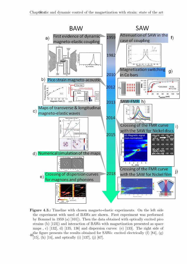
Chapter 4Static and dynamic control of the magnetization with strain: state of the art
Figure 4.3.: Timeline with chosen magneto-elastic experiments. On the left sidethe experiment with used of BAWs are shown. First experiment was performedby Bommel in 1959 (a) [101]). Then the data obtained with optically excited picostrains (b) [123]) and interaction of BAWs with magnetization presented as spacemaps , c) [132], d) [135, 136] and dispersion curves: (e) [133]. The right side ofthe figure presents the results obtained for SAWs: excited electrically (f) [84], (g)[15], (h) [14], and optically (i) [137], (j) [67].46

4.2 Dynamic strain
Despite all these articles, a remaining problem was the lack of direct time-resolvedmeasurements of magnetization precession excited with SAWs. The signal detectedin the IDT set-ups raised many questions and controversy about the origin of SAWattenuation and velocity change with field.. The theory developed among others byDreher et al. and Thevenard et al. even if describing well SAW data needed to bealso confronted to magnetic data.
4.2.2.2. Optical excitation of SAWs
To allay those doubts researchers headed towards optically excited SAW, sincethe implementation of optical time-resolved measurements with electrically excitedSAWs was not trivial due to the synchronization of the laser pulses to the electri-cal signal. In this technique a laser pulse is split in two, one is used to generateSAW and the other to detected magnetization precession. In one of the first papersJanusonis et al. [67] used the transient grating technique to excite monochromatic4 GHz SAWs on a Nickel film deposited on a MgO substrate (Fig. 4.3 (j)), with theFaraday rotation detection performed in the center of the excitation area. The mag-netization precession was detected. Additionally, strain was monitored through thetransient diffraction. The strongest magnetization precession signal occurred exactlyat the intersection of the estimated FMR frequency curve with the SAW frequency.Moreover, the continuously tuned wavelength of the SAW gives the possibility toperform dispersion measurement. The dispersion of the SAW overlapped with themagnetization dispersion, which justified the origin of the magnetization precession.Later in the same experimental scheme, parametric magnetization excitation wasshown including second harmonic generation [138].Another approach for monochromatic SAW generation was proposed by Yahagi[137]. An array of Nickel elliptical thin discs on Silicon substrate was heated upwith pump pulses (Fig. 4.3 (i)). The principle of SAW excitation is the same asfor the transient grating, only here the spacing between the discs determined thewavelength of the excited SAW. This allows to excite SAWs of much smaller λ thanthe transient grating technique. Changes in magnetization were probed with themagneto-optical Kerr effect and acoustic waves were probed using reflectivity. Sim-ilar features as in Janusonis’ paper were observed: magnetization precession showedup when the FMR frequency coincides with the SAW frequency. Moreover, theycompared the results with the one obtained for a non-patterned Nickel films and afilm of Aluminium. For those samples, the modes correlated to SAWs disappeared.Considering all these articles one part still missing is the unquestionable evidenceof the magnetization precession excitation with electrically excited SAWs. Thiscan be done only by employing one of the optical techniques for the time resolveddetection. Another thing which has never been shown is the excitation of spin wavesin tightly focused laser beam configuration for which SAWs will not be assigned to aunique wavevector. For this configuration only BAWs were used for magnetizationexcitation.
47

Chapter 4Static and dynamic control of the magnetization with strain: state of the art
These two points will be addressed in this work. The experimental part of the thesisis divided into two sections. In one SAWs are excited with an IDT (Fig. 4.4 (a))and in the second one they are excited optically with the tightly focused laser beamtechnique (Fig. 4.4 (b)). With the IDT we have studied magnetization precessionexcited in a GaMnAs film with 4 frequencies 151, 301, 452 and 603 MHz of SAWswith plane wavefront. The magnetic field was applied along a hard axis to matchthe FMR frequency with SAWs. The studies were performed for different powers ofSAWs and for a few temperatures.In conrast, for the optical approach, broadband circular SAWs were generated with acentral frequency between 1 and 2.5 GHz depending on the substrate. The power ofthe SAWs could not be tuned as easily as with IDT. However, due to the simplicity ofthe implementation, we could test many specimens. The experiment was performedat room temperature. Therefore, the studied samples were ferromagnetic metalson transparent substrates. In both cases, magnetization precession was detectedwith use of the time- and space- resolved magneto-optical Kerr effect. In case ofthe electrically excited SAWs, the electrical detection of the SAW attenuation andphase change was also possible.
Figure 4.4.: Schemes of two experimental set-ups for SAWs generation: (a) elec-trically and (b) optically.
48

5. Experimental techniques
Table of content
5.1 Magnetic characterization5.1.1 Cavity FMR5.1.2 Broadband FMR (BBFMR)5.1.3 Vibrating-sample magnetometer (VSM)
5.2 Time and frequency domain detection of spin waves5.2.1 Faraday effect5.2.2 Magneto-optical Kerr effect5.2.3 Voigt effect5.2.4 Brillouin light scattering spectroscopy (BLSS)
5.3 Detection of Surface acoustic waves - Photo-elastic effect5.4 Materials
5.4.1 GaMnAs5.4.2 Ferromagnetic metals
The magnetic samples require a good characterization of magnetic properties todetermine if they are suitable for a desired experiment. We need to know param-eters such as the Curie temperature, the magnetization saturation, the magneticanisotropy of the sample and, what is critical from the point of view of this work,the Ferromagnetic resonance (FMR) frequency dependence on the magnetic field.Here we describe the FMR techniques for the two group of samples used: cavityFMR (for ferromagnetic semiconductors) and broadband FMR (for ferromagneticmetals). Our experiment assumes the excitation of the magnetization precession inthe range of a few hundreds of MHz to the GHz regime. In order to resolve dynamicchanges of the magnetization, we used an optical technique (the Kerr magneto-optical effect), since it offers a great spatial resolution, which is important for theexcitation of spin waves with the high frequency SAWs. In magneto-optical Kerreffect (MOKE), the rotation of polarization of the reflected light is detected and itis proportional to the magnetization. The measurement of polarization changes canbe used not only to detect the magnetization precession but also SAWs through thephoto-elastic effect as shown later in this chapter.
49
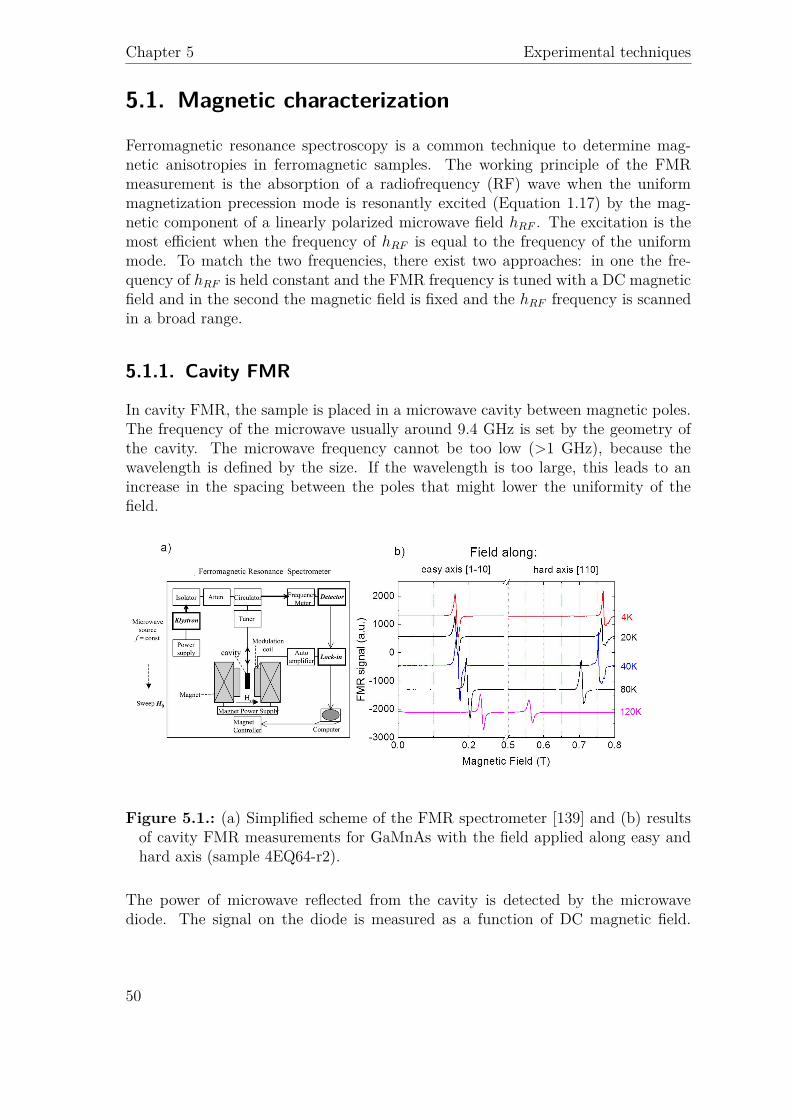
Chapter 5 Experimental techniques
5.1. Magnetic characterization
Ferromagnetic resonance spectroscopy is a common technique to determine mag-netic anisotropies in ferromagnetic samples. The working principle of the FMRmeasurement is the absorption of a radiofrequency (RF) wave when the uniformmagnetization precession mode is resonantly excited (Equation 1.17) by the mag-netic component of a linearly polarized microwave field hRF . The excitation is themost efficient when the frequency of hRF is equal to the frequency of the uniformmode. To match the two frequencies, there exist two approaches: in one the fre-quency of hRF is held constant and the FMR frequency is tuned with a DC magneticfield and in the second the magnetic field is fixed and the hRF frequency is scannedin a broad range.
5.1.1. Cavity FMR
In cavity FMR, the sample is placed in a microwave cavity between magnetic poles.The frequency of the microwave usually around 9.4 GHz is set by the geometry ofthe cavity. The microwave frequency cannot be too low (>1 GHz), because thewavelength is defined by the size. If the wavelength is too large, this leads to anincrease in the spacing between the poles that might lower the uniformity of thefield.
Figure 5.1.: (a) Simplified scheme of the FMR spectrometer [139] and (b) resultsof cavity FMR measurements for GaMnAs with the field applied along easy andhard axis (sample 4EQ64-r2).
The power of microwave reflected from the cavity is detected by the microwavediode. The signal on the diode is measured as a function of DC magnetic field.
50

5.1 Magnetic characterization
The detection sensitivity is increased by modulating the DC magnetic field at a lowfrequency of a few hundreds of Hz (Fig. 5.1 (a)). To find the in-plane anisotropyof the sample, the magnetic field is applied at different angles in the sample plane.The sample is rotated around the normal to the plane. The out-of-plane anisotropyis investigated by applying the magnetic field along different directions from thenormal to the film to the film plane.Typical curves of cavity FMR measurements are presented in Fig. 5.1 (b), here forGaMnAs. These data were taken by Jürgen Von Bardeleben and Teyri Amarouchein INSP. The field was applied along the easy and hard axes for a few temperatures.We can see that the field needed to match the two frequencies is lower for the easyaxis. The in-plane anisotropy constants: K2‖ and K4‖ of the GaMnAs sample werefound, by performing the cavity FMR measurements for more DC magnetic fieldorientations and then by fitting the found FMR fields with Equation 1.15. Thelinewidth also inform us about the sample homogeneity.Although FMR can also be used to measure the magnetization Ms(T ) [140], aftercalibration by a sample with know Ms(T ), we have instead used a more convenienttechnique, the vibrating sample magnetometer (VSM) to measure Ms(T ).The FMR technique provides great sensitivity since the sample is placed in thecavity. Moreover, the sample can be measured at low temperature. For samplesthat do not require low temperature measurement we rather use the broad-bandFMR technique recently developed in our group
5.1.2. Broadband FMR (BBFMR)
In BBFMR, the sample is placed on a coplanar waveguide [141]. This is a transmis-sion line consisting of three metallic planar electrodes running parallel to each otheron a dielectric slab. The central line is the conductive line, with two ground lines onboth sides separated by air. The RF electric current IRF creates the RF magneticfield µ0hRF ∼= µ0
IRFw
(w is the width of the conducting line) around the line [142].This can excite the magnetization precession in the sample and as a result of thetime varying magnetic flux a microvoltage is created in the transmission line [144].To monitor this effect, changes of the impedance are measured. Since the measuredchanges are small and need to be measured at high frequency (>1 GHz), a VectorNetwork Analyzer (VNA) is used. It measures the transmission and reflection ofelectromagnetic waves, which are described by scattering parameters:
S =(S11 S12S21 S22
)(5.1)
S11 and S22 are the reflection parameters, and S12, S21 are the transmission param-eters. We have mainly worked with the transmission parameter (S12), which can be
51

Chapter 5 Experimental techniques
Figure 5.2.: (a) Schematic of the set-up for Broadband FMR measurement [143].In (b) and (c) are presented the real and imaginary component of the scatteringparameter ∆S12 for a 100 nm thick Nickel film. The power of IRF was 0 dBm.
expressed as [145]:
S12 = e−γ0(l1+l2)P (1− Γ2)1− P 2Γ2 (5.2)
where P = e−γls , l1 + l2 is the total length of the part of the waveguide not occupiedpart by the sample (Fig. 5.2 (a)). The sample length is ls. Γ is the impedanceratio: Γ = Z−Z0
Z+Z0, it is equal to zero when the sample is not loaded, otherwise the
waveguide impedance is modified from Z0 to Z and the propagation constant (γ0without sample) becomes γ.In the experiment, the sample lies with the magnetic layer side down onto the waveg-uide, which is placed between the poles of a magnet. Two ports of the waveguideare connected with SMA (SubMiniature version A) coaxial cables to the VNA. ThehRF field is scanned from 300 kHz to 8 GHz (maximal frequency range of Rohde-Schwarz ZVA8 Vector Network Analyzer) for a chosen static magnetic field value.The impedance mismatch between the waveguide and the 50 Ω cables and VNAcan give rise to a S12 parameter. That is why it needs to be calibrated when thesample is not positioned on the waveguide. The measured calibrated ∆S12 = S12
S12(ref)parameter has real and imaginary components, which correspond to the magneticsusceptibility[145]. From the measured curves <∆S12(B) and =∆S12(B) we can ob-tain the dependence of the FMR frequency on the magnetic field. On some samples(usually thicker than 100 nm) we can easily fallow the dependence of the resonance
52

5.2 Time and frequency domain detection of spin waves
frequency with the applied field down to low field values < 20 mT (Fig. 5.2 (b) and(c)). For thin samples or some of the FeGa samples, the poor quality of the signalmakes it difficult to determine the resonance frequency at low field. The BBFMRwas developed for INSP by I.S. Camara to characterize ferromagnetic metals. Withthe established set-up we can measure the samples only at room temperture, thatis why it was not used for the ferromagnetic semiconductors.
5.1.3. Vibrating-sample magnetometer (VSM)
VSM is a technique to measure the sample magnetization. The first VSM devicewas built and used in 1959 by Simon Foner [146]. The working principle is based onthe Faraday induction law. The sample is mounted on a rod, vibrating in a constantand uniform magnetic field. The alternating flux induces a voltage in the pick-upcoils, which is directly proportional to the magnetization. Varying the externalmagnetic field, a full hysteresis cycle can be obtained. In VSM devices equippedwith cryogenic temperature control, the Ms(T ) dependence can be measured. Weused this technique to measured Ms(T ) of GaMnAs and to obtain the anisotropyconstants from cavity FMR and fFMR(B) dependence (Equation 1.15 and 1.18 ).
5.2. Time and frequency domain detection of spinwaves
5.2.1. Faraday effect
Magneto-optical effects illustrate the interaction of light with matter, where thepolarization of light can be affected by the magnetic medium. One of these effectswas discovered by Michael Faraday in 1845 [147]. He observed that the plane oflinearly polarized light is rotated upon propagation in a dielectric medium under anexternally applied magnetic field (Fig. 5.3).A similar effect, but for reflection of light from a magnetic medium was found 30years later by J. Kerr. Those two effects were named after their discoverer. Theobserved rotation of light polarization is due to magnetic circular birefringence anddichroism. The material has two different refractive indices for left and right cir-cularly polarized light. Let us consider linear polarized light propagating in theFaraday configuration i.e. with the ~k vector along the magnetic field or the magne-tization. It can be written as the combination of left and right circularly polarizedlight. The (σ±) circularly polarized light propagating along the z axis is written asfollows:
~E = E0(~ex + ~eye
±iπ2)ei(kz−ωt) (5.3)
53

Chapter 5 Experimental techniques
Figure 5.3.: Illustration of the Faraday effect. The state of the polarization of theincident beam is changed upon propagation in a magneto-optical medium.
The plus (minus) is for left (right) circularly polarized light. The polarization as-sociated with the electric field vector rotating anticlockwise is called left circular.Let us assume the incident light polarization along ~x. A linear polarization can bedecomposed into the sum of a right and left circularly polarized light. The ~E vectorof light propagating in the sample can then be written as:
~E = 12E0 ( ~ex + i ~ey) e
i
(2πn+λ
z−ωt)
+ 12E0 ( ~ex − i ~ey) e
i
(2πn−λ
z−ωt)
(5.4)
where n+ and n− are the refractive indices for left and right polarized light and λ isthe light wavelength in the vacuum. The above equations after some trigonometricaltreatment can be presented in the following form [148, 149]:
~E = E0ei( 2πn̄
λz−ωt)
(~ex cos δ2 −
~ey sin δ2
)(5.5)
where n̄ = 12 (n+ + n−) and δ = 2π
(n+−n−
λ
)z. From this we can immediately
see that the linearly polarized light will be rotated due to to the propagation inthe circular birefringence medium. The angle of Faraday rotation depends on the
54

5.2 Time and frequency domain detection of spin waves
optical path and is simply given as:
ϑF = δ
2 = π(n+ − n−
λ
)L (5.6)
where L is the length of the dielectric medium. For a transparent, paramagneticmaterial the Faraday rotation angle is directly proportional to the applied magneticfield. To define the indices n+ and n− we need to employ Maxwell equations:
~∇× ~E = −∂~B
∂tFaraday’s law of induction (5.7)
~∇× ~B = µ0ε0∂ ~E
∂t+ µ0 ~J Ampere’s law (5.8)
~∇ · ~E = ρ
ε0Gauss’s law (5.9)
~∇ · ~B = 0 Gauss’s law for magnetism (5.10)
~J is the current density and ρ is the charge density. The current density is givenas: ~J = ∂~P
∂t+ ~∇× ~M , ~P is the electric polarization which for a linear materials has
a linear dependence on the electric field. Inserting this formula into Ampere’s law(Equation 5.8) we get:
~∇× ~H = ∂ ~D
∂t, (5.11)
where µ0 ~H = ~B − µ0 ~M and the electric displacement ~D = ε0 ~E + ~P = ε0εr ~E, εris the relative dielectric tensor. Now, combining 5.11 with Faraday’s induction law(Equation 5.7) and assuming that ~M varies slowly as compared to the period oflight, we will get:
∇2 ~E −∇(∇ · ~E
)= µ0ε0εr
∂2 ~E
∂t2(5.12)
55

Chapter 5 Experimental techniques
Looking for plane wave solutions, we obtained:
n2 ~E − ~n(~n · ~E
)= εr ~E (5.13)
where ~n = ~k cω
is the complex refractive index (the light phase velocity in thematerial is lowered by the factor n with respect to the vacuum). Since light is atransverse wave (~k ⊥ ~E) the equation above is simplified to:
n2 ~E = εr ~E (5.14)
For cubic crystals [78] (p24):
εr = ε
1 −iQmz iQmy
iQmz 1 −iQmx
−iQmy iQmx 1
(5.15)
Q is the Voigt constant which is proportional to the magnetization Ms existing orinduced by the field. The dielectric tensor is related to the electronic transitionsfrom the valence band [150]. The transition excited with left and right circularpolarization makes m-electron ( m is the magnetic quantum number) obey a differentselection rule ∆m = +1 for left and ∆m = −1 for right helicity of photon. In ourcase the magnetization ~m ‖ z (mz = 1), then εr is given as:
εr = ε
1 −iQ 0iQ 1 00 0 1
(5.16)
Then from Equation 5.14 the refractive indices are:
n2± = ε(1±Q) (5.17)
The eigenmodes are ~E0 = E0 (~ex ± i~ey), which are the left and right circular polar-izations of light. The Faraday angle can now be explicitly defined:
ϑF = πL
λ<[√εQ]
(5.18)
Here we assumed that Q is small (∼ 0.03 [78]), thus n± = n0(1 ± Q2 ), where n0 =√
ε. When linearly polarized light passes through a magnetic medium not only itspolarization plane undergoes a rotation, but it also becomes slightly elliptical. Theellipticity is related to = [
√εQ], that is to magnetic circular dichroism. The typical
value of Faraday rotation for Ni and Co is 35 deg/µm (data for λ = 830 nm) [151],for GaMnAs the value is around 6 deg/µm(data for λ = 800 nm) [152].
56

5.2 Time and frequency domain detection of spin waves
5.2.2. Magneto-optical Kerr effect
In magneto-optical Kerr effect (MOKE), which is the effect we use in this work, threedifferent configurations to probe three perpendicular magnetization components canbe distinguished (Fig. 5.4). In the polar Kerr (PMOKE) configuration, the compo-nent perpendicular to the sample plane is probed. Longitudinal and transverse Kerreffects are sensitive to the in plane magnetization components: respectively paralleland transverse to the light incidence plane.
Figure 5.4.: Three configurations of MOKE.
Here we will take a closer look at PMOKE. The linearly polarized light arrivesperpendicular to the vacuum/ferromagnet interface. The amplitude of the reflectedbeam is described by the Fresnel coefficients. As it was discussed in the previousparagraph, it is convenient to decompose the linear polarization into right and leftcircular polarizations since those two have different refraction indices. The ratiobetween the reflected
(~ER
)and incident
(~EI
)light is given by [149, 153]:
r = EREI
= −n− 1n+ 1 (5.19)
For us ER is the sum of left and right circular polarization of light (Equation 5.4),with n+ and n− respectively. Hence, if the incident beam is defined as 5.4, thereflected wave is given as:
~ER = 12EI
−n+−1n++1 −
n−−1n−+1
i[−n+−1n++1 + n−−1
n−+1
] ( ~ex~ey
)ei(−
2πλz−ωt) ≈ EI
(−n0−1n0+1
−i n0Q(n0+1)2
)(~ex~ey
)ei(−
2πλz−ωt)
(5.20)
The polarization of the reflected beam will be rotated and additionally the state ofpolarization will be changed. To see it clearly we can define the ratio r between thetwo orthogonal polarization components:
r = EyEx
(5.21)
57

Chapter 5 Experimental techniques
The rotation of the major axis of the ellipse is due to the phase difference of the tworeflected circular components and this is related to the magnetic circular dichroism,thus for a semi-infinite material:
ϑK = < [r] = <[in0Q
n20 − 1mz
](5.22)
The ellipticity results from the inequality of the amplitude of the two reflecte circularpolarization components. This is related to the magnetic circular birefringence andwe have:
ψK = = [r] = =[in0Q
n20 − 1mz
](5.23)
The mz component was added at the end to stress again the magnetization depen-dence of the two. In this work we used static MOKE to characterize the magnetichysteresis cycle of the samples (Fig. 5.10) and the time-resolved MOKE (TRMOKE)to study magnetization dynamics. For most magnetic materials, the Kerr rotationangle is of the order of magnitude 0.1− 1 deg [154].
5.2.3. Voigt effect
In the case of perpendicular orientation of the light wavevector with respect tothe magnetization direction, two secondary effects have to be considered: magneticlinear birefringence (MLB) and magnetic linear dichroism (MLD) called togetheras Voigt effect. Let us analyze the situation where light arrives normal to samplesurface. We assume that the sample is in-plane magnetized since, this applies to themajority of thin films as it was discussed in the first chapter. For cubic crystals thedielectric tensor can be expanded up to quadratic terms in the components of ~m inthe following form [78]:
εr = ε
1 −iQmz iQmy
iQmz 1 −iQmx
−iQmy iQmx 1
+
W1m2x W2mxmy W2mxmz
W2mxmy W1m2y W2mymz
W2mxmz W2mymz W1m2z
(5.24)
where W1 and W2 are the quadratic Voigt constants. For an isotropic materialW1 = W2 and since there is no experimental evidence that W1 6= W2 in GaMnAs,
58
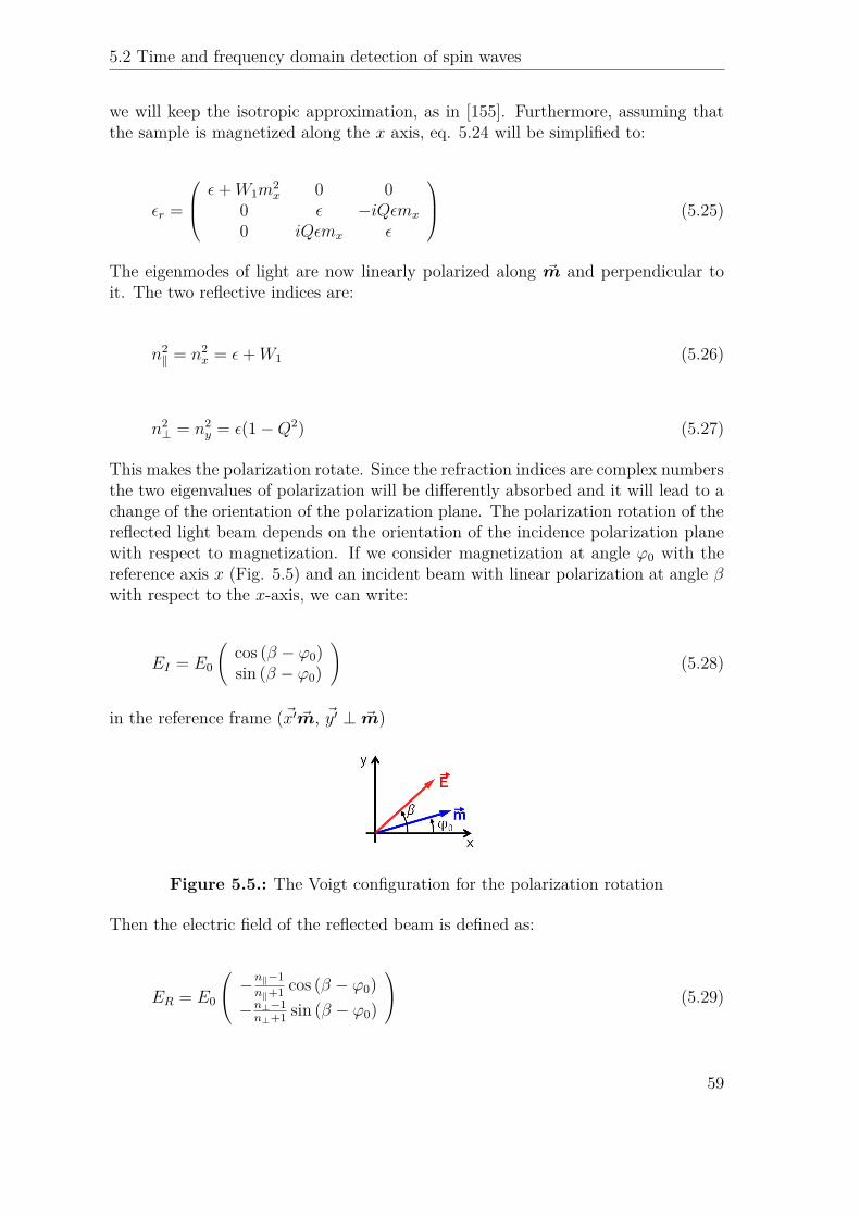
5.2 Time and frequency domain detection of spin waves
we will keep the isotropic approximation, as in [155]. Furthermore, assuming thatthe sample is magnetized along the x axis, eq. 5.24 will be simplified to:
εr =
ε+W1m2x 0 0
0 ε −iQεmx
0 iQεmx ε
(5.25)
The eigenmodes of light are now linearly polarized along ~m and perpendicular toit. The two reflective indices are:
n2‖ = n2
x = ε+W1 (5.26)
n2⊥ = n2
y = ε(1−Q2) (5.27)
This makes the polarization rotate. Since the refraction indices are complex numbersthe two eigenvalues of polarization will be differently absorbed and it will lead to achange of the orientation of the polarization plane. The polarization rotation of thereflected light beam depends on the orientation of the incidence polarization planewith respect to magnetization. If we consider magnetization at angle ϕ0 with thereference axis x (Fig. 5.5) and an incident beam with linear polarization at angle βwith respect to the x-axis, we can write:
EI = E0
(cos (β − ϕ0)sin (β − ϕ0)
)(5.28)
in the reference frame (~x′ ~m, ~y′ ⊥ ~m)
Figure 5.5.: The Voigt configuration for the polarization rotation
Then the electric field of the reflected beam is defined as:
ER = E0
−n‖−1n‖+1 cos (β − ϕ0)−n⊥−1n⊥+1 sin (β − ϕ0)
(5.29)
59

Chapter 5 Experimental techniques
Projection on the vectors (~e‖, ~e⊥ ), ~e‖ being the unit vector along the incidentpolarization ~E, gives:
ER = E0
−n‖−1n‖+1 cos2 (β − ϕ0)− n⊥−1
n⊥+1 sin2 (β − ϕ0)
sin (β − ϕ0) cos (β − ϕ0)(n‖−1n‖+1 −
n⊥−1n⊥+1
) (5.30)
As it was for the Kerr rotation, the ratio between the two polarization componentsr = E⊥
E‖will give the rotation of the polarization angle:
∆β =
(n‖ − n⊥
)sin 2 (β − ϕ0)
n⊥n‖ − 1 +(n‖ − n⊥
)cos 2 (β − ϕ0)
(5.31)
Assuming small polarization rotation angle ( n‖n⊥
≈ 1), the formula 5.31 can be writtenin more general form:
∆β ≈ n‖ − n⊥n⊥n‖ − 1 sin 2 (β − ϕ0) = 1
2
W1ε
+Q2
n20 − 1 sin 2 (β − ϕ0) , (5.32)
We define the complex number V = <[
12
W1ε
+Q2
n20−1
]+ i=
[12
W1ε
+Q2
n20−1
]. The real part
determines the Voigt polarization rotation and the imaginary part the ellipticity.The Voigt effect is maximized for the incoming polarization oriented at 45 deg tothe static magnetization. The polarization rotation due to the Voigt effect is usuallymuch smaller than the one due to the PMOKE (if W � Q2 then the Voigt effectis proportional to Q2 which is much smaller then Q since Q � 1). However, theVoigt and Kerr effects depend on the light wavelenght have strong dependence onλ, which may be chosen to maximize or to minimize one of them. It was shownthat for GaMnAs, the ratio between the two effects can be modified by the factorof 10 by changing the wavelength [156]. For ferromagnetic metals the λ-dependenceis very small [157].
5.2.4. Brillouin light scattering spectroscopy (BLSS)
BLSS is a different approach to detect spin waves. A photon with energy ~ωI of theprobing beam is inelastically scattered by a magnon of energy ~ωm (Fig. 5.6 (a)).As a result of energy and momentum conservation, one has [158]:
~ωS = ~ (ωI ± ωm) (5.33)
60

5.2 Time and frequency domain detection of spin waves
~~kS = ~(~kI ± ~km
)(5.34)
the energy of the scattered photon is increased (+ sign) or decreased (- sign), de-pending on whether a magnon is annihilated or created. The probability of the twoprocesses depends on the temperature when only thermal magnons are present. Us-ing BLSS one can also probe coherent magnons, i.e. magnons excited by an antenna.From the point of view of classical physics, it can be understood as the refraction ofthe light on a moving phase grating, induced by the spin wave. Then the Dopplershift of the frequency will correspond to the frequency of the spin wave [159].
Figure 5.6.: (a) Diagram of one of the two scattering processes. (b) The workingprinciple of a tandem Fabry-Perot interferometer [159].
By detecting the scattered photons one can directly measure the frequency of thespin waves. This light frequency change is commonly detected with the use of a tan-dem Fabry-Perot interferometer which can spectrally filter the light scattered fromthe sample (only the light whose wavelength fulfills the constructive interferometrycondition is transmitted) (Fig. 5.6 (b)).One advantage of BLSS is that it can provide in plane wave-vector resolution bychanging the incidence angle of light. Therefore the spin wave dispersion curve canbe measured. This is also possible with scanning TRMOKE.The biggest difference between these two is that BLSS is a frequency domain tech-nique while TRMOKE is measured in the time domain. However, with BLSS onecan also perform time domain studies but only for a one chosen, fixed frequency[160].Recently microfocused BLSS with the spatial resolution of the order of 1 μm wasused to study spin waves in patterned ferromagnetic materials. In that case thewavevector resolution is partially lost.The frequency reachable with BLSS is in the range of 0.2 GHz - 1 THz [159], whichcovers the spectrum of spinwaves for ferromagnetic materials (a few GHz) but notfor antiferromagnetic materials (usually >1 THz). Moreover, it can be used to
61

Chapter 5 Experimental techniques
detect acoustic waves by playing with excitation/detection light polarization [161],e.g. it was used to measure the frequency of the surface acoustic waves in a 1 µmthin optical fiber [162]. BLSS is generally a good choice to study propagating spinwaves modes, while TRMOKE is an excellent technique to investigate the uniformspinwave mode. In this work we used the later method, since it is devoted to theuniform mode.
5.3. Detection of Surface acoustic waves -Photo-elastic effect
In paragraph 5.2 we showed that the magnetic order in the materials can lead tobirefringence, which might be detected as a change of a polarization of the reflectedlight beam. We will show here that birefringence can also originate from strain. Inthis case, the variation of the permittivity tensor due to strain can be expressed asfollows [63]:
∆εil = −εijPjkmnεkl∂um∂xn
, (5.35)
where Pjkmn is the elasto-optic tensor with values ranging from 0.1-0.3. For anisotropic medium it is given as:
∆ε = −ε2
P11Sxx + P12 (Syy + Szz) (P11 − P12)Sxy (P11 − P12)Sxz(P11 − P12)Sxy P11Syy + P12 (Sxx + Szz) (P11 − P12)Syz(P11 − P12)Sxz (P11 − P12)Syz P11Szz + P12 (Sxx + Syy)
(5.36)
Here we use the Voigt notation for the elast-optic tensor. We will consider now thecase of a Rayleigh surface acoustic waves with ~kSAW ‖ ~x excited electrically by anIDT. The only non zero strain components at the surface are Sxx and Szz . Hencethe permittivity tensor will be simplified to:
∆ε = −ε2
P11Sxx + P12Szz 0 00 P12 (Sxx + Szz) 00 0 P11Szz + P12Sxx
(5.37)
Now we can define two refractive indices for light propagating along the z axis:
{nx =
√ε+ ∆εxx
ny =√ε+ ∆εyy
(5.38)
62

5.4 Materials
Since the strain is of the order of 10−5, we assume that the perturbation of theindices is small and can be expressed as follows:
nx = n(1− εP11Sxx+P12Szz
2
)ny = n
(1− εP12(Sxx+Szz)
2
) (5.39)
Using formula 5.32 developed for the Voigt effect, the polarization rotation due tothe SAW is written as:
∆βstrain = <[n3(P11 − P12)Sxx
2 (n2 − 1)
]sin 2β (5.40)
From equation 5.40 we can calculate the polarization rotation due to the photo-elastic effect for a given strain, if we know the elasto-optic constants. For GaAs itis around 1.2 µrad for Sxx = 10−5 and |P11 − P12| = 0.06 (for λ = 870 nm) [163].The polarization rotation is sensitive to the in-plane strain component Sxx. On thecontrary, with the interferometric measurements which is the most common methodfor SAW detection, only the out-of-plane displacement is probed (Uz). However, itprovides very high sensitivity: a pico-meter surface displacement can be observedwith it. We used the PE effect to detect SAW excited electrically and interferometricmeasurement were used for metallic samples with SAW generated optically.
5.4. Materials
In this thesis, two different groups of materials were used. For the studies with elec-trically excited SAWs we worked with GaMnAs (Fig. 5.7 (a)), which is a good mate-rial for PMOKE measurement, because of the relatively low out-of-plane anisotropy.Moreover, the FMR frequency can be easily tuned with the magnetic field. However,it required low temperature (T<100 K). Because of this requirement and the factthat it cannot be grown on a transparent substrate, it was not used in the secondproject where acoustic waves are excited through the substrate with a tightly focusedlaser beam and magnetization variations are detected on the other side (Fig. 5.7(b)). This set-up specification makes another group of materials perfect candidates:ferromagnetic metals that have a Curie temperature well above room temperatureand that absorb very well visible light. More details on these materials will be givenbelow.
63

Chapter 5 Experimental techniques
Figure 5.7.: Schemes of two experimental set-ups for SAW generation (a) electri-cally and (b) optically.
5.4.1. GaMnAs
GaMnAs joins together two important properties: ferromagnetic and semiconduc-tor, used in the information technology for data storing and processing respectively.This material gave a green light for developing spintronic devices. The concept ofGaMnAs relies on replacing of few Ga atoms from the GaAs lattice by Mn atoms.Comparing the electronic structure of the two atoms (Ga: 3d104s2p1, Mn: 3d54s2),one can see that the 3d shell will now be only half filled but also, what is moreimportant for the magnetic order, due to the lack of 4p valence electron, one hole isintroduced. This weakly bound hole mediates the interaction between the localizedMn spins and aligns them ferromagnetically. The first GaMnAs sample was grownby H. Ohno in 1996 [164]. In order to incorporate a few percents of Mn atoms, thegrowth temperature needs to be below 300°C, which is at least two times lower thanthe growth temperature of GaAs (∼600°C). However, the lowered growth tempera-ture leads to the reduction of the film quality, introducing defects such as interstitialMn and As in antisites and post-growth annealing needs to be achieved in order toremove part of the defects [165]. The Curie temperature (TC) is related to the con-centration of Mn ions. TC increases monotonically with the effective concentrationof Mn (xeff ) and hole concentration (p) [166]. Up to now, the highest reported Curietemperature for GaMnAs is 191 K [167], which is still far from room temperature.According to the theory developed in 2000 [34], room temperature TC should beachieved for xeff = 12.5% and p = 3.5× 1020cm3. However, now we know that thisconcentration will be very hard to achieved, since Mn-atoms can also occupy theinterstitial position in the lattice and couple antiferromagnetically to the Mn in Gaposition [168].Despite its low TC, GaMnAs is a good test-bench material because its magnetic andmagneto-elastic properties can be tuned by the epitaxial strain, and the Mn andhole concentrations.In this work, we have studied one GaMnAs sample. GaMnAs was our first choice,since our group has a great experience with it, e.g. the former PhD student Syl-vain Shihab developed TRMOKE set-up to study magnetization precession and to
64

5.4 Materials
determine the spin stiffness constants with the use of Kerr and Voigt effects. Thesample was carefully architectured by Aristide Lemaître from C2N laboratory tohave a strong in-plane anisotropy. He has grown 45 nm thick GaMnAs film on (001)GaAs substrate, therefore with built-in epitaxial strain (see Eq. 3.7). After growth,the sample was annealed for 16h at 200°C. The Mn concentration was xeff = 5%and Curie temperature TC = 130 K.
Figure 5.8.: (a) The saturation magnetization as a function of temperature ob-tained using VSM. (b) The calculated FMR frequency versus magnetic field alongthe hard magnetic axis [110] for different temperatures.
Two factors determined the conditions of our measurement: Ms and the frequencyof SAW. With the VSM we have measured the saturation magnetization dependenceon the temperature, showing that the magnetization decreased by a factor of 2 fromT=0 K to T=100 K (Fig. 5.8 (a)). Lower magnetization means lower MOKE signal.The second important quantity is the FMR frequency calculated from the anisotropyconstants measured with cavity FMR as a function of the magnetic field. The curvesfor 7 temperatures are presented for a field applied along the hard axis (Fig. 5.8(b)). They possess the same features: first the FMR frequency decreases untilmagnetization is aligned with the field and after that it increases again. We havechosen to work with SAW frequency below 600 MHz (wavelength > 5μm) compatiblewith our spatial resolution. Therefore we need to lower the FMR frequency by anin-plane field as shown here in order to match the SAW frequency.
5.4.2. Ferromagnetic metals
We have studied four ferromagnetic films for different reasons. Galfenol, an alloy ofFe and Ga was chosen because of its very high magnetostriction. It was reportedthat substituting 19 % of Fe by Ga-atoms in thin epitaxial layers, makes the mag-netostriction coefficient increase 10 times (λFe100 = 0.2× 10⁻⁴ → λFeGa100 = 2.6× 10⁻⁴)
65

Chapter 5 Experimental techniques
[169]. This is a very high value for thin layers. We used two different FeGa filmsone was prepared by Mahmoud Eddrief at INSP and another one by Rocio Ran-chal at Universidad Complutense de Madrid. The latter one was prepared to havean in-plane uniaxial magnetic anisotropy. Our second choice was Nickel due to lowFMR frequency which could be easily made equal to the SAW frequency even in zeromagnetic field. This sample was made by Loïc Becerra at INSP. Moreover, we alsoinvestigated Cobalt which is likewise known as a good magnetostrictive material.
5.4.2.1. Nickel
Previous studies have revealed that the magnetic properties such as saturation mag-netization, coercive field, hysteresis squareness, static strain of magnetic films de-pend on their thickness and on which substrate they were deposited [170, 171]. Inthis work, we have studied different thicknesses of Nickel films (20, 100 and 300 nm)sputtered on glass, since the substrate had to be transparent.
Figure 5.9.: (a) The BBFMR characteristics for the three Nickel films. (b) Hys-teresis cycles for 20 nm Nickel sample measured with static longitudinal MOKE.
In Figure 5.9 (a) the FMR resonance frequency obtained from BBFMR (Fig. 5.2 (b)and (c) for the 100 nm sample) is plotted versus magnetic field for the three Nickelsamples. These data clearly show that a resonance frequency below 1 GHz in zeromagnetic field can be obtained for the 100 nm thick Nickel sample. That is whywe mainly worked with this sample as you will see later in the experimental part(Chapter 7). Samples have a small in-plane anisotropy as it is presented in graph(b) of Figure 5.9.
66

5.4 Materials
5.4.2.2. FeGa
We studied the two FeGa sample. The first sample was a 88 nm thick Fe0.8Ga0.2filmgrown by molecular beam epitaxy on a SrTiO3 substrate (STO). Galfenol was cappedwith a 10 nm Au layer to protect it from oxidation. With longitudinal MOKEwe found that the sample is isotropic in the plane (Fig. 5.10). Broadband FMRmeasurements showed that the resonance frequency in zero magnetic field is around3.8 GHz, which is quite high compared to the Nickel samples.
Figure 5.10.: FeGa on STO substrate. The hysteresis cycles from longitudinaltaken along 4 different axes.
The second sample was a 120 nm Fe72Ga28 layer sputtered on a 500 µm Sapphiresubstrate cut along the C- plane (0001). The two buffer layers of Molybdenum weredeposited: 14 nm on Sapphire/FeGa interface and 7 nm on top of the FeGa layer.The details on the sample preparation can be found here in ref: [172]. This samplewas prepared to have an in-plane uniaxial magnetic anisotropy. The longitudinalKerr cycles are presented in Fig. 5.11 (a), showing a strong uniaxial anisotropy.
67

Chapter 5 Experimental techniques
Figure 5.11.: The hysteresis cycles of FeGa on Sapphire substrate measured withlongitudinal MOKE and (b) BBFMR characteristic with magnetic field appliedalong the hard axis.
To find the precession frequency dependence on magnetic field we performed BBFMR(Fig. 5.11 (b)). The FMR frequency was never lower than 1 GHz (fFMR(μ0H=17mT)=1.2GHz). However, we knew that with a Sapphire substrate we can aim for higher SAWsfrequency than with glass due to its higher Rayleigh velocity.
5.4.2.3. Cobalt
The last sample was 100 nm Cobalt on Sapphire. This sample was prepared bysputtering by Stefan Suffit at University Paris VII. The layer was not uniform,showing many micro-holes (Fig. 5.12 (a)). We used two different substrates butwe could not get rid off of the holes. The sputtering conditions were probablynot optimal. Nevertheless, we obtained a good MOKE signal (Fig. 5.12 (b)). Itwas found that Cobalt layer was isotropic. In the experiment using optical SAWexcitation, we did not experience any difficulties due to these holes.
68

5.4 Materials
Figure 5.12.: Microscope image of Cobalt on Sapphire. Here shown with differentcap layers which were tested to enhanced the Kerr signal. (b) The hysteresismeasured with longitudinal MOKE configuration. (c) Result of the BBFMR fora field from 0 to 83 mT.
The precession frequency at zero magnetic field was around 2 GHz (arrow in Fig.5.12 (c)).
69

6. Spatial and dynamical control ofmagnetization with electricallyexcited surface acoustic waves
Table of content
6.1 Phase synchronization6.1.1 Experimental set-up6.1.2 Jitter measurement6.1.3 Lock-in detection of the optical signal6.1.4 IDT design6.1.5 Phase between the optical and electrical signal
6.2 Detection of the magneto-acoustic signal6.2.1 Burst shape
6.3 Polarization dependence studies6.3.1 Methodology6.3.2 Field dependence6.3.3 The magnetization precession excitation efficiency versus SAW frequency6.3.4 Phase of the TRPR signal6.3.5 Temperature dependence6.3.6 Power dependence6.3.7 Back-action of the magnetization precession on SAW - SAWFMR6.3.8 Spatial mapping of the magnetic and acoustic waves
6.4 Perspectives
In this chapter, the results of magnetization precession excited in a thin film of(Ga,Mn)As with the use of electrically generated SAWs will be presented. This isthe first time that magnetization precession is detected optically in this type of sys-tem. For that purpose, we developed a unique experimental set-up and the methodto distinguish magnetic and elastic contributions from MOKE and PE effect, respec-tivly. The results show the resonant magneto-elastic coupling, in good agreementwith the model. The IDT design used allowed us to generate SAWs at four differentfrequencies 151, 301, 452 and 602 MHz. We will discuss the efficiency of detectionof the acoustically-induced resonant magnetization dynamics at these frequencies.This project was led in close collaboration with Jean-Yves Duquesne.
71

Chapter 6Spatial and dynamical control of magnetization with electrically excited surface
acoustic waves
6.1. Phase synchronization
Time-resolved measurements require stable phase locking between the excitationand the detection signals. In the case of magneto-optical measurements, with mag-netization precession excited by electrically generated SAWs, the common solutionto synchronize the optical probing pulses and the electrical signal is a master-slaveconfiguration. The laser frequency and the frequency of the electrical wave are im-posed by a common clock. This can be done with laser systems equipped with thesynchro-lock function, where the laser cavity length is tuned with a movable mirrormounted on a piezoelectric stage. The laser repetition rate frequency has to be amultiple of 10 MHz to make it suitable for a phase-locked loop. For the acousticwave excitation, the clock of the pulse generator is synchronized with the commonclock using the 10 MHz input [173].
Figure 6.1.: Experimental set-up
However, this technique requires expensive devices. In this thesis, we proposed asimpler, alternative and widely accessible approach. Herein, we used a laser signalto create the electrical signal. The laser frequency was picked up with a photodiode,then this signal was converted with RF components to higher frequencies. Addi-tionally it was shaped in a form of burst a few hundred ns long which were sent tothe IDT. Because the SAW frequency fSAW was built from the laser repetition rate(fL) a stable phase lock between the SAW and the optical probe pulses was assured.
72

6.1 Phase synchronization
6.1.1. Experimental set-up
For the purpose of this project an existing pump-probe set-up, developed by SylvainShihab was modified. The operating frequency fL ∼= 75 MHz of the Ti:Sapphirelaser was picked up by a slow Silicon photodiode (PDA10A-EC, Thorlabs) posi-tioned behind the backside polished mirror (Fig. 6.1). Then the electronic signalwas processed for the SAW excitation. The harmonics of the fundamental fL weresufficiently lowered with a 50dB rejection bandpass filter. Next, multiples of thelaser frequency n×fL (n = 2, 4, 6, 8) were obtained with various RF multipliers. Togenerate ∼ 151 MHz, 301 MHz and 602 MHz we have used n/2 number of doublers,except for the 452 MHz where a × 6 multiplier was used. After each multiplicationof the frequency, the signal was filtered with a band-pass filter (Fig. 6.2).
Figure 6.2.: RF connections for generation of harmonic frequencies of the laserrepetition rate. RF amplifiers were used because the multipliers required a veryspecific RF input power. They may also introduced other harmonics, that is whya band-pass filter (BPF) was placed at the output.
The part of the light reflected from the mirror (nearly 100%) was sent to an APEpulse picker. This device is based on the acousto-optic effect. It allows to dividefL by an integer number N, where N is 2 - 260 000. The efficiency of this processdepends on the chosen N, for N higher than 40, an efficiency of 80% can be obtained.Every laser pulse at the frequency fL /N can be delayed by 12 ns with a 6×60 cm longmotorized optical delay line. The maximum temporal resolution was ∼ 0.5 ps. Thelaser probe beam was spatially filtered with a 20 µm pinhole, positioned betweentwo lenses in the plane conjugated with the sample plane. It ensured very highspatial stability on the sample surface during scanning the delay line. The beamwas expanded 1.7 times, to fully cover the entrance pupil of the Mitutoyo (LCDPlan Apo 20x, NA=0.4) objective, as a result the spot size of ∼ 1 µm (at FWHM)was obtained. The probe beam fluence was about 1.5 mJ
cm2 and the wavelength wasλ = 722 nm.Before delivering the n×fL electronic signal to the IDT, it was shaped into bursts.
73

Chapter 6Spatial and dynamical control of magnetization with electrically excited surface
acoustic waves
For this purpose the signal was mixed with a square wave generated with the pulsegenerator (81150A Keysight Pulse function arbitrary noise generator) at the pulsepicker frequency fL /N. In order to generate pulses at the pulse picker frequency, thepulse generator was externally triggered via the pulse-monitor electronic output ofthe pulse picker (the maximum accepted frequency for the Keysight pulse generatorwas 120 MHz). Thus both the carrier frequency and the envelope frequency werecommensurate with fL . That also protected the signal in the envelope from drifting.Moreover, with the pulse generator we could delay the bursts with respect to theoptical signal. The maximum delay time was equal to the burst period, typically afew µs. Finally, the produced signal was applied to the IDT after a 40 dB amplifier.The highest reachable power was around 36 dBm (∼4 Watts), it depended on thecarrier frequency used and the electronic configuration. The typical strains are inthe order of 6×10⁻⁵(for 100 mW of input power) [60, 174].
6.1.2. Jitter measurement
To quantify the stability of the set-up we have performed jitter measurements. Jit-ter is defined as the short-term variation of the transition edge positions in timefrom their ideal values [175, 176]. There exist many types of jitter which help tocharacterize the timing performance. Exemplary types of the deterministic jitterare: Period jitter, Cycle to Cycle jitter, Time interval error (TIE) jitter. The Periodjitter and Cycle to Cycle jitter refer to the variation of the clock period, measuredeither as the deviation of a large number of cycles from the ideal (average) periodvalue or as the difference of the adjacent cycles across the given number of cycles.When the ideal clock source is available, the TIE jitter can be measured, which isthe difference between the location of the ideal edge and the signal edge (Fig. 6.3).
74

6.1 Phase synchronization
Figure 6.3.: Three main types of the deterministic jitter: Cycle to cycle, Periodand TIE jitter.
In the case when the ideal clock signal is used as the reference source to generatethe signal then a more appropriate name for TIE jitter is the edge-to-reference jitter[175]. This jitter was the most relevant for us. Therefore, to estimate the jitterwe displayed on the oscilloscope (LeCroy HDO9204) traces of the square signalgenerated with the pulse generator and the laser pulses picked up with the fastphotodiode (mounted for this purpose in the set up) at fL /300 (Fig. 6.4). Thesignal was triggered with the laser pulses. The jitter was measured with the delayoscilloscope function which measures the delay between the trigger and the signaledge. The delay was measured over 1000 samples. The most meaningful value whichdescribes the jitter is the standard deviation which was found to be equal to 13.1ps, which is much lower than 1% of a period of the lowest SAW period used in thiswork.
75

Chapter 6Spatial and dynamical control of magnetization with electrically excited surface
acoustic waves
Figure 6.4.: Time traces of the laser pulses and square wave at fL /300 with thedistribution of the TIE jitter.
6.1.3. Lock-in detection of the optical signal
Linearly polarized laser pulses reflected from the sample return through the same ob-jective and are delivered to the balanced optical bridge detector (Thorlabs PDB150A)(Fig. 6.1). It consists of two photodiodes, on which the two orthogonal polariza-tion components are projected by a polarizing beam splitter. Then the difference isamplified.The signal from the bridge was next detected with the Lock-in amplifier (7270General-Purpose DSP Lock-in Amplifier) at the frequency of the mechanical chop-per. The chopper was placed just before the slow photodiaode to modulate the burstat 541 Hz (Fig. 6.1). This configuration allows to measure the polarization rotationlower than 1 µrad.The polarization rotation was calculated from the following formula:
δβ = sChopLock−in
4Rsps, 1dLock−in(6.1)
where sChopLock−in is the signal detected at the chopper frequency, sps, 1dLock−in is the signaldetected on one diode at the pulse picker frequency and R is the conversion ratioequal to to 1.3 for a bridge gain 106. The sChop, 1dLock−in was used not only to find thepolarization rotation but also to normalize the time domain signal since the lightintensity was not the same for all the delay line positions because of the light diver-gence. The details on the derivation of Formula 6.1 can be found in the AppendixA.
76

6.1 Phase synchronization
6.1.4. IDT design
The specific design of an IDT allows to excite efficiently certain overtone harmonicsof the fundamental frequency (f0). In our case the frequencies were imposed by thesynchronization strategy. When a certain design is chosen the parameters determin-ing which frequencies are excited are the digit periodicity, the number of digits andthe metallization ratio. The architecture of the IDTs used in this work was elabo-rated with the help of Jean-Yves Duquesne. The frequency response of the IDT iscalculated from the so-called δ-function. Here we will briefly describe it based onan example of the basic IDT design presented in Fig. 6.8 (a). The full descriptioncan be found in [63]. The alternating voltage applied to the IDT creates a gradientof the electric field which is the highest at the edges of the electrodes where chargesare accumulated. The distribution of the electric field can be illustrated by the twoδ-functions of the same polarity associated with each tooth (Fig. 6.5). This modelcan be simplified using only one equivalent δ-function at the center of an electrode.Hence the time domain response of the IDT is given as [63, 177]:
h(t) =N−1∑n=0
(−1)nAnδ(t− tn) (6.2)
and in the frequency domain Equation 6.2 is:
H (ω) =N−1∑n=0
(−1)nAne−iωtn (6.3)
where An is the amplitude of each delta and tn is the time interval from the nthelectrode to the detection point: tn = t0 + n d
υ= t0 + n π
ω0.
77

Chapter 6Spatial and dynamical control of magnetization with electrically excited surface
acoustic waves
Figure 6.5.: Illustration of the electric field distribution as the δ-function in a uni-form IDT [63, 177].
Then the condition for constructive summation is ωω0
= m, where m can only takeodd numbers as it is the Fourier transform of a square wave. Thus only the oddmultiple of the fundamental frequency will be sustained. From Equation 6.3, we canfind that the response of the IDT for the frequency detuned from the synchronousfrequency f0 is in the form of a sinc function:
Hn (f) = AnNsinXm
Xm
Xm = Nπ
2f −mf0
f0(6.4)
The boundaries of the bandwidth are located where Hn (f) goes to zero. This is forN = 2 f0
∆f with ∆f = f −mf0, which can be written as:
∆ff0
= 2N
(6.5)
From 6.5 we can directly see that the bandwidth is inversely proportional to thenumber of teeth. It means that increasing the N we narrow the bandwidth (Fig.6.6). Moreover, the value of N also governs the transient time. It increase with N,which means that to obtain a plateau, the burst width has to be long enough but itcannot be too long if we want to have a clear separation from the electromagneticradiation on the receiving IDT as it will be shown later.These simple calculations show that the even harmonics cannot be excited with ahighly symmetric structure. In a paper by Schülein [178] the design for odd and even
78

6.1 Phase synchronization
harmonics excitation was proposed. He showed that double, triple, quadruple andless efficiently sextuple (fm = m×f0, m = 1, 2, 3, 4, 6) harmonics can be generated.The fundamental frequency was defined by the longest periodicity. The possibilityto generate even and odd harmonics allows to characterize the investigated systemwith discrete SAWs frequencies laying close to each other. We adopted this so-calledsplit-52 design to our experiment (Fig. 6.8 (b)). The highest frequency was chosenfor the corresponding wavelength to be compatible with a good spatial resolutionwith the probe beam. The diameter of the beam spot was around w=1 µm (fullwidth at half maximum). Hence the λSAW for quadruple frequency was selected asλSAW = υR
8×fL = 4.6 µm > 4 × w. Thus the period of the IDT had to be designed tofit to the laser frequency (d = υR(T )
2fL ). Since the IDT period depends on the Rayleighvelocity which varies with temperature and one of our restriction was to work in thetemperature range of 3-100 K (Ga,Mn)As, the IDT had to be well tailored. TheIDT period was designed for υR at the center of the temperature range. To ensureefficient work in the wide temperature range the number of digits could not be toohigh. We tested two sets of IDT on GaAs: one with N=15 and the other with N=25.We found that the -3 dB bandwidth was ∆fN=25 ' 3.9 MHz and ∆fN=15 ' 6.1 MHz.
Figure 6.6.: (a) Frequency span of the IDT with N=15 and N=25 measured witha VNA, for a 0 dBm excitation power. (b) The frequency response of the IDTwith 25 digits.
However, the power of excited SAWs was 7 dB lower for the N=15 therefore wedecided to work with the narrower bandwidth design (N=25) (Fig. 6.6 (a)). InFigure 6.7 we plotted the center frequency for four harmonics vs temperature. Theviolet line in the graphs indicates the multiple of the laser frequency. For the scalewe put on the right the ∆fN=25 bandwidth. As you can see the deviations from themaximal frequency are far below the bandwidth.
79

Chapter 6Spatial and dynamical control of magnetization with electrically excited surface
acoustic waves
Figure 6.7.: Temperature dependence of the central frequency of the four harmon-ics excited with the IDT of split 52 - design. The horizontal, purple line indicatesthe multiple of the laser frequency.
Note that there exists another approach for wide frequency SAWs excitation. Insteadof decreasing the number of teeth, a small linear variation of the IDT periodicity(period changed by 10% in a 400 µm long IDT structure) can be introduced [179].As the result, the bandwidth is enlarged by the frequency chirp.The (Ga,Mn)As sample was made by A. Lemaître, see Chapter 5 Section 4.1 forits full characteristic. Than the sample was processed by Loïc Becerra at INSPby optical lithography with the lift-off method to deposit the IDTs. First the 2×2mm2 mesa of the 45 nm thick GaMnAs film on GaAs was prepared by the wetetching technique. Then the whole sample was covered with a 1.2 µm thick positivephotoresist by a spinning technique. Next, a UV laser beam traced the patternaccording to the IDT design and the irradiated resist is removed. Finally a 45 nmthick Aluminium layer was evaporated forming the IDTs and contacts on GaAs.In the last step, the non-irradiated photoresist is removed with Acetone and theAluminium remained only in the places illuminated by the laser.
80

6.1 Phase synchronization
Figure 6.8.: (a) The most common design of IDT. The metallization ratio is definedas 2wd
λ0(b) Final IDT 52 design and (c) an image of the sample taken with an optical
microscope.
Two pairs of IDTs were deposited: one for the propagation of SAW along the easyaxis and the other along the hard axis of (Ga,Mn)As (Fig. 6.8 (c)). The SAWFMRstudies obtained before for the same sample showed that these the resonance fieldand attenuation amplitude were similar [180]. We have chosen to work with ~kSAWalong the easy axis because these IDTs were more efficient. Moreover, we usedthe SAWFMR measurement to check the resonance field and the conditions for thelinear regime of magnetization precession.
6.1.5. Phase between the optical and electrical signal
To define the phase between the SAWs and laser pulses we placed the fast photodiode(Thorlabs DET10A) in front of the sample, so the laser pulses were visualized on theoscilloscope with the electronic bursts. The burst and laser signals were triggeredon the latter one. We found that there was a fixed delay τf ' 657 ns between thelaser pulse and the first rising edge of the burst, due to the different velocities of
81

Chapter 6Spatial and dynamical control of magnetization with electrically excited surface
acoustic waves
the electric and optical signals (typically υe ' 0.7c). Based on this measurementwe found an empirical formula for the delay (∆τ) of the acoustic waves in order todefine their spatial position between two IDTs:
∆τ = τP −a
υR− τf + τw/2, (6.6)
where τP is the burst period (typically a few μs), aυR
described the arrival time tothe detection point and τw is the burst width (usually 400ns) (Fig. 6.9). Here weput τw/2, which is the situation where the center of the burst is detected.
Figure 6.9.: The determination of the phase between the SAW’s bursts and laserpulses was essential to detect the signal.
6.2. Detection of the magneto-acoustic signal
We spent about one year building and characterizing the set-up. Now the dataobtained for the (Ga,Mn)As sample will be presented. Figure 6.10 shows typicaltime-resolved polarization rotation (TRPR) measurements taken at 60 K for thefour IDT excitation frequencies 151, 301, 452 and 602 MHz available in our sample.The probe beam was polarized at 60° with respect to ~kSAW . The frequency of thedetected signal was found to be equal to the excitation frequency. The signal-to-noise ratio is good for all frequencies and we do not see a big influence of the decreaseof λSAW to the beam spot size ratio. Furthermore, to illustrate how high frequenciescan be measured, the result for excitation with 904 MHz is also presented in Fig.6.10 (e). The signal still looks very good and probably we can aim for 1 GHz, eventhough in this case λSAW < 3 µm. We see also 452 MHz in the excitation signal,because we did not have an electronic filter for this frequency since we did not plan
82
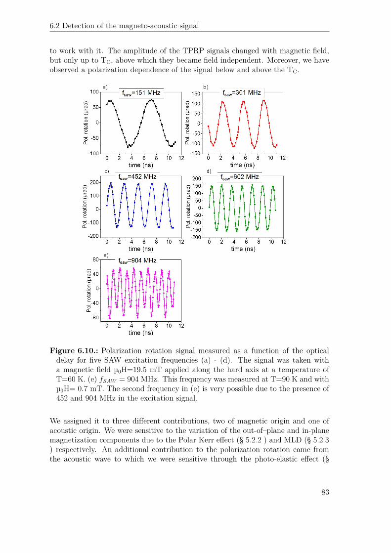
6.2 Detection of the magneto-acoustic signal
to work with it. The amplitude of the TPRP signals changed with magnetic field,but only up to TC, above which they became field independent. Moreover, we haveobserved a polarization dependence of the signal below and above the TC.
Figure 6.10.: Polarization rotation signal measured as a function of the opticaldelay for five SAW excitation frequencies (a) - (d). The signal was taken witha magnetic field µ0H=19.5 mT applied along the hard axis at a temperature ofT=60 K. (e) fSAW = 904 MHz. This frequency was measured at T=90 K and withµ0H= 0.7 mT. The second frequency in (e) is very possible due to the presence of452 and 904 MHz in the excitation signal.
We assigned it to three different contributions, two of magnetic origin and one ofacoustic origin. We were sensitive to the variation of the out-of–plane and in-planemagnetization components due to the Polar Kerr effect (§ 5.2.2 ) and MLD (§ 5.2.3) respectively. An additional contribution to the polarization rotation came fromthe acoustic wave to which we were sensitive through the photo-elastic effect (§
83

Chapter 6Spatial and dynamical control of magnetization with electrically excited surface
acoustic waves
5.3). Hence the measured polarization rotation can be described by the followingexpression:
δβ(β, H, t) = Kδθ(H, t) + 2V δϕ(H, t) cos 2(β−ϕ0(H)) +PESxx(t) sin 2β, (6.7)
Figure 6.11.: Coordinate system for polarization rotation measurements.
where PE is the photo-elastic constant which was defined in section 5.3 and forisotropic materials PE = <
∣∣∣n3P44n2−1
∣∣∣, δθ(H, t) and δϕ(H, t) are the dynamic functionsof magnetization orientation given as:
δθ(H, t) = δθMax cos (2πfSAW t+ ψθ) (6.8)
δϕ(H, t) = δϕMax cos (2πfSAW t+ ψϕ) (6.9)
In contrast to the MLD and PE effects, PMOKE is independent of the polarizationorientation. On the other hand, the PE effect does not depend on the magneticfield. Therefore we can use these dependencies to distinguish the three effects fromeach other.We expected to see two physical regimes: linear and nonlinear. The linear regime iswhen the magnetization precession amplitude is small and we observe it oscillatingonly at a single frequency equal to fSAW (Equations 6.8 and 6.9). This is the casefor most of the data taken at 60 K at a low power. For higher temperatures, itis easier to enter the nonlinear regime, where the magnetization oscillates with thelarge amplitude at 2fSAW or in case of the magnetization switching at fSAW/2.
84

6.2 Detection of the magneto-acoustic signal
6.2.1. Burst shape
Firstly, to confirm that the detected signal was due to the SAWs we measured theamplitude of the magneto-acoustic signal measured in TRPR as a function of theelectrical burst delay ∆τ . For each delay, the signal was measured as a function ofthe optical delay, the amplitude was simply extracted by fitting the curve with thesingle sine function. Here, the purpose was not to disentangle magnetic and acousticsignals, that is why scans were taken for only one probe polarization (β = 30°)and at one value of the magnetic field (µ0H=20 mT). The features of the opticallymeasured signal were compared with the signal detected electrically (red solid line)with the second IDT through the inverse piezo-electric effect and visualized with anoscilloscope. In the electrically detected signal the electromagnetic radiation 400 nsburst arrived first, traveling at the speed of light. After ttrans = d
υR∼= 730 ns, the
acoustic echo arrived. The Rayleigh velocity was found around υR = 2780 m/s. Thewidth of the acoustic burst was bigger because of the lower velocity, which increasesthe transition time through the 25 digits. The burst-shaped excitation, with shortenough on time ensured that those two signals were well separated from each other.
Figure 6.12.: (b) The red curve is the time trace detected electrically and the twodotted lines represent the amplitude of the TRPR signal detected in two placeson the sample marked in the scheme in (a). The data was taken at 60 K with amagnetic field of 19.5 mT. (c) is the image of the IDT and the beam spot, wherethe data represented by empty dots in (b) was taken. The time scans for chosenelectronic delays are plotted in (d) (vertically off-set for clarity).
85

Chapter 6Spatial and dynamical control of magnetization with electrically excited surface
acoustic waves
First the probe beam was positioned 108 µm from the receiving IDT (Fig. 6.12(a) and (b) - empty circles) - the precise position of the spots on the sample wasfound with an imaging system not shown in the set-up scheme (Fig. 6.12 (c)).Each point of the empty circle curve in Fig. 6.12 (b) indicates an amplitude ofthe oscillations observed in TRPR (Fig. 6.12 (d)). We can see that the shape ofthis curve corresponds to the acoustic echo detected with the IDT and it is almostoverlapped with it since it was detected nearly at the same place. The rise and falltime is defined by the time the SAW excited with the last digits pair needs to travelthrough the whole IDT. The duration of a steady state of the burst was proportionalto the excitation pulse width reduced by the rising and falling time. Moreover, wecan conclude that the electromagnetic radiation does not trigger the preccession.Then the probe beam was moved 67 µm from the emitting IDT (black spot in Fig.6.12 (a)) and an identical profile was found, but this time closer to the excitationmoment (Fig. 6.12 (b) full circles). The ∼ 20% change of the amplitude of the peakis due to attenuation of the SAW by the magneto-elastic coupling. Moreover, wecan find the Rayleigh velocity, since we know the distance between the two detectionpoints: υR = 2880 m/s. The small deviation from the value detected electricallyoriginates from the measurement condition, in optically detected SAWs, the burstprofile is discretized and it is difficult to give an exact arrival time.
6.3. Polarization dependence studies
6.3.1. Methodology
To study the magnetization precession excited with the SAWwe performed a series of12 ns - delay line time scans, probing the center of the burst for different orientationsof the incoming linear polarization. Then we plotted the measured signal versus thepolarization for each delay line position and we fitted it with the following expression:
δβ = Fθ +Gϕ cos 2β +HϕS sin 2β, (6.10)
where
Fθ(H, t) = Kδθ(H, t)
Gϕ(H, t) = 2V δϕ(H, t) cos 2ϕ0(H)HϕS(H, t) = 2V δϕ(H, t) sin 2ϕ0(H) + PESxx(t)
(6.11)
Figure 6.13 (a) shows the TRPR signal for 6 orientations of the incoming beampolarization. The curves were taken for a SAW excitation frequency fSAW = 301 MHz
86

6.3 Polarization dependence studies
at T= 60 K. The clear evidence of polarization dependence of the TRPR signal isalso presented in the Figure 6.13 (b), for which data were extracted from the previousgraph at a fixed time indicated by the green dashed line (Figure 6.13 (a)). The datapoints were fitted with the function 6.10. For zero magnetic field we see mainlythe PE contribution of sin 2β, since the magnetization is along the easy axis and ifour experiment is well aligned the precession will not be excited (Equation 3.10).Moreover, when the polarization is at 0°, it is along kSAW and we are not sensitive tothe PE effect. The application of the magnetic field clearly modified the signal (redcurve). The offset that appears corresponds to PMOKE which does not dependon polarization and the change of the phase is due to the presence of the Voigteffect. By performing the fitting for each time and fitting the extracted parameters(Fθ(H, t), Gϕ(H, t), HϕS(H, t)) with a sinusoidal function of fSAW we can obtain theamplitudes of Kerr (fθ(H), Fθ(H, t) = fb + fθ(H) cos(ωSAW t − ψf )) and the Voigt(gϕ(H), Gϕ(H, t) = gb+gϕ(H) cos(ωSAW t−ψg)) rotation and the photo-elastic partmixed with the Voigt effect (hϕS(H), HϕS(H, t) = hb +hϕS(H) cos(ωSAW t−ψh)) ata given field value.
Figure 6.13.: (a) TRPR signal taken for six probe orientations of the polarizationat µ0H=6 mT, fSAW=301 MHz, T=60K. (b) The polarization dependence of thesignal at fixed optical delay (green dashed line in Fig. 6.13(a)) for two values offield.
6.3.2. Field dependence
To find how the parameters vary with the field we performed the polarization studiesfor field up to 36 mT. The amplitudes fθ(H), gϕ(H) and hϕS(H) are presented inFig. 6.14 (a).
87

Chapter 6Spatial and dynamical control of magnetization with electrically excited surface
acoustic waves
Figure 6.14.: (a) Field dependence of the three parameters fθ, gϕ and hϕS forfSAW=302 MHz and T= 60 K. To keep measurement time low we limited thepolarization studies only to 6 polarizations. However, we checked that fit qualitywas not lower than for 18 polarization orientations. The time needed to take thecurves from (a) is 6.5 h. (b) Calculated fθ, gϕ and hϕS components. The valuesof fitting parameters used are K=18 mrad, V=0.8 mrad, PE=0.77 rad with Sxx =5.3×10⁻⁵. The arrow in the graph indicates the field value for which fprec = fSAW .
Before discussing the obtained field dependence we will explicit the relations of theseamplitudes with the magnetization and the strain components:
• fθ = KδθMax - the amplitude of out-of-plane magnetization precession multi-plied by the Kerr constant,
• gϕ = V δϕMax cos 2ϕ0 - the amplitude of in-plane magnetization precessionmultiplied by the Voigt constant and by cosine of 2ϕ0, ϕ0 is giving the orien-tation of ~mwith respect to ~kSAW ,
• hϕS - represents a mixed contribution of the amplitude of the in-plane dynam-ical magnetization and the longitudinal component of the SAW.
fθ (H) increases monotonously up to ∼ 23 mT, where fSAW is expected to be theclosest to fFMR, and decreases again to zero. gϕ(H) has two maxima with anintermediate position at 16 mT for which cos 2ϕ0(H) = 0 and the magnetizationis oriented at 45° to the easy axis (Equation 6.11) . In hϕS(H) signal we cansee the two contributions, the constant offset is directly proportional to the fieldindependent Sxx strain component and the signal on top of it to the Voigt effect.To confirm the fθ(H), gϕ(H) and hϕS(H) field dependence, we calculated the samecomponents using the coupled equation system (Equation 3.9) and the measuredsample parameters (Section 5.4.1). The results are presented in Fig 6.14 (b). Theyare in very good agreement with the data measured experimentally. To obtaincomparable peak’s height and width, a small dispersion of the uniaxial in-planeanisotropy was introduced.
88

6.3 Polarization dependence studies
As shown, the TRPR signal decomposition into the three elements is a techniquewhich allows us to distinguish in-plane and out-of-plane dynamical magnetizationcomponent and Sxx strain component. The results obtained experimentally agreewith the analytical solutions. Hence we used this approach to study the dependenceof the magnetization precession amplitude upon various factors such as the SAWsfrequency and power, and temperature.
6.3.3. The magnetization precession excitation efficiency versusSAW frequency
When the magneto-acoustic coupling occurs part of the SAW power is absorbed bythe magnetic layer, when the magneto-acoustic coupling occurs and it is used toexcite magnetization precession. It can be expressed as Pabs = −ωSAW
2 =~h∗RFχ
~hRF ,where χ is the tensor of magnetic susceptibility [13, 180, 114]. This general formulaindicates that we can expect some fSAW dependence of the absorbed power. Indeedthis behavior was demonstrated experimentally by monitoring electrically the SAWamplitude attenuation versus magnetic field [180, 181, 13], it was also verified byus, see Fig. 6.22. Measuring optically the amplitude of magnetization precessionwe expected to observe a similar behavior: the largest amplitude oscillations for thehighest fSAW . In Figure 6.15 the three extracted components fθ, gϕ and hϕS areplotted for 151, 301, 452 and 602 MHz excitation SAW frequencies.
Figure 6.15.: Comparison of the field dependence of fθ, gϕ and hϕS for the fourexcitation frequencies.
We have excited the 4 frequencies with equal voltage amplitudes (PRF = 24 dBm∼=251mW), however it does not mean that the excited strains had the same amplitudesince the IDT did not have a flat characteristic as you can see in Fig. 6.6 (b) and6.7. Fortunately, we were able to use the PE (baseline of hϕS(H)), which is a verygood indicator of the amplitude of strain Sxx(as it will be shown after) to normalizethe fθ and gϕ curves. Such normalized fθ showed a strong peak around 22.5 mT forall frequencies. This was because there was little dependence of the resonance field
89

Chapter 6Spatial and dynamical control of magnetization with electrically excited surface
acoustic waves
on SAW frequency since the FMR curve is very steep for the frequency range below1 GHz (Fig. 5.8 (b)). Moreover, it is seen that only the amplitude for 602 MHzdiffer from the rest. The gϕ curves coincide for three frequencies 151, 301 and 602MHz. The amplitude of gϕ is comparable with fθ. Thus, the motion of the magne-tization vector is that of an ellipse |δθMax| � |δϕMax| , because K > V . The static~m position ϕ0 reached 45° around the same field value (∼16 mT), which is a goodevidence of the temperature stability of our system and measurement repeatability.For 452 MHz, the two bumps were strongly asymmetric. It is from the hϕS curvesdependencies that the fSAW dependency was better observed. The baseline for hϕSwas not adjusted to show the strain amplitude is not very different for the fourfrequencies. Again the curve for 452 MHz strays from the rest which may suggestthat the experimental conditions for this frequency were different than for the rest.
6.3.4. Phase of the TRPR signal
The data which were not discussed up to now, but carry as important informationsas the signal amplitude, is the phase. The relative phase of Fθ, Gϕ and HϕS wasobtained from the same fit used before to determine the variations of the precessionamplitude with field. The three components have different phases as can be seen inFigure 6.16 (a), where Fθ(H, t), Gϕ(H, t) and HϕS(H, t) are plotted for µ0H= 6mT .
Figure 6.16.: (a) Time traces of Fθ, Gϕ and HϕS for µ0H= 6mT . (b) Dependenceof Fθ, Gϕ, HϕS phases on magnetic field for 301 MHz.
The extracted phase versus field is shown in Figure 6.16 (b) versus field. The phaseof certain components shows very interesting features. The change of phase of theHϕS component is almost flat. This phase is difficult to analyze since we have thecontribution of the two effects. In the two other components, we observe changesrelated to the magnetic field. The phase of Fθ changes monotonously by π. In thecase of small damping we expect an abrupt change of phase by π at the point wherefSAW = fFMR(H). A higher damping (α = 0.05) and small misalignment of themagnetic field in respect to the hard axis can make this change smoother. A similar
90

6.3 Polarization dependence studies
π phase changed was observe by Janusonis et al. [182], where the magnetizationprecession was excited with SAWs generated with the transient grating technique.In the phase of Gϕ(H, t) we also observe a π changed, however much sharper. Thischange is due to the rotation of the orientation of the static magnetization. Whenit traverses 45°, the phase changed by π since in our fitting procedure we forced theamplitude to be positive by adjusting the phase ψg.
6.3.5. Temperature dependence
At temperatures close to TC, the magnetization orientation can be tuned more easily,with lower fields than at low temperature. The anisotropy field of the (Ga,Mn)Assample decrease with increasing the temperature (§ 5.4.1). In Fig. 6.17 we presentfθ, gϕ components normalized by the PE effect and hϕS components for 151 MHzat T= 60 K and 90 K.
Figure 6.17.: fθ, gϕ normalized by the PE effect and hϕS component for 60 K and90 K, versus magnetic field for the sample excited with SAW at 151 MHz. Theexcitation power was 25 dBm.
The temperature influence is very well illustrated by the gϕ component. For 90 Kwe observe only a single, sharp peak. This peak can be identified as the second(high field) peak in the data taken for 60K. It means that even small field (∼1 mT)can bring magnetization at 45°. Similar features are observed in fθ and hϕS signals.The peaks are much shifted to the lower fields. This is explained by the fact thatthe FMR frequency depends strongly on temperature as it was shown in Fig. 5.8.Indeed here we see a confirmation of that. The resonance field is lower by around15 mT for 90 K.In Figure 6.18, the results for three other frequencies are shown. The dependencelooks similar to one observed for 151 MHz. The excitation power for 90 K waschosen to be relatively low (17 dBm= 50 mW) to avoid nonlinear effects, which willbe discussed in the next paragraph.
91
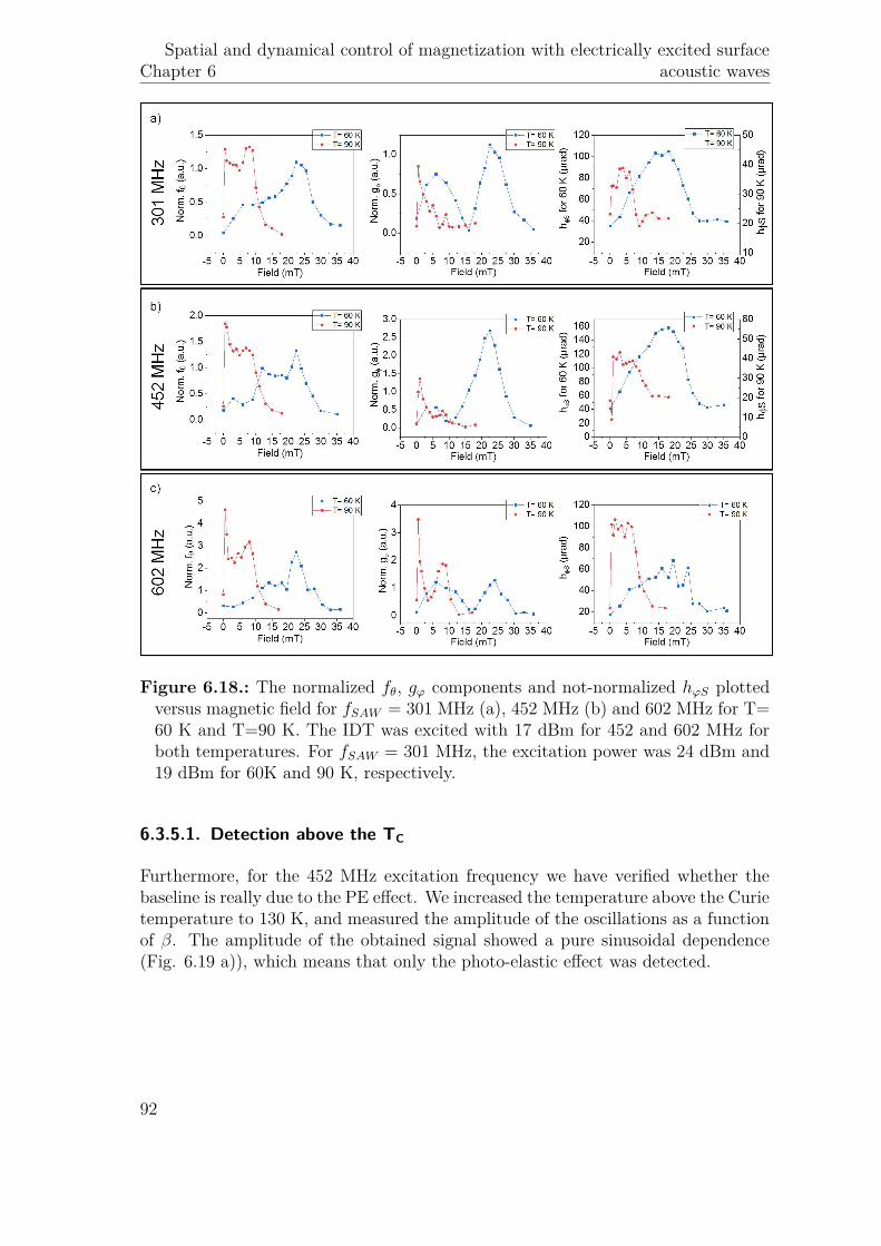
Chapter 6Spatial and dynamical control of magnetization with electrically excited surface
acoustic waves
Figure 6.18.: The normalized fθ, gϕ components and not-normalized hϕS plottedversus magnetic field for fSAW = 301 MHz (a), 452 MHz (b) and 602 MHz for T=60 K and T=90 K. The IDT was excited with 17 dBm for 452 and 602 MHz forboth temperatures. For fSAW = 301 MHz, the excitation power was 24 dBm and19 dBm for 60K and 90 K, respectively.
6.3.5.1. Detection above the TC
Furthermore, for the 452 MHz excitation frequency we have verified whether thebaseline is really due to the PE effect. We increased the temperature above the Curietemperature to 130 K, and measured the amplitude of the oscillations as a functionof β. The amplitude of the obtained signal showed a pure sinusoidal dependence(Fig. 6.19 a)), which means that only the photo-elastic effect was detected.
92

6.3 Polarization dependence studies
Figure 6.19.: (a) Amplitude of photo-elastic signal measured above the TC forfSAW= 452 MHz. (b) Amplitude of hϕS signal versus magnetic field at T= 60 Kand for fSAW= 452 MHz. The horizontal line indicates the amplitude of the signalfrom the left graph.
The amplitude of the signal extracted from Fig. 6.19 a), is plotted on top of thehϕS field dependence curve taken for the same excitation power and frequency at60 K (Fig. 6.19 b)). The baseline perfectly overlaid with the PE signal measuredabove TC. This clearly confirmed our predictions, that no magnetic contribution isdetected above the TC and that only below TC, 2 other components are detected.If we would know the PE for GaAs at low temperature, we could deduce the strainamplitude from Fig. 6.19 (a).
6.3.6. Power dependence
We also tested the efficiency of the precession excitation for different SAW powers.For electrically excited SAW, the power can be easily adjusted by tuning the voltagewith which the IDT is excited. In Figure 6.20 we present Fθ(t), Gϕ(t) and HϕS(t)signals for fSAW = 452 MHz, for three excitation powers: 17, 24 and 30 dBm.The Fθ(t) and HϕS(t) signal amplitudes increase with increasing SAW amplitude.However, the most interesting signal is presented in Figure 6.20 (b), where Gϕ(t)for the highest power oscillated at two frequencies: 452 MHz and double of thisfrequency. Since the 904 MHz frequency is not observed in HϕS(t) and disappearsat high magnetic field, it can clearly be ascribed to the nonlinear precession ofmagnetization and not to the nonlinear excitation of SAW [183]. The componentoscillating at 904 MHz is also present in the Fθ(t) signal but because of the ratiobetween two amplitudes is smaller ( f904MHz
θ
f904MHzθ
+f452MHzθ
× 100 = 11%; g904MHzϕ
g904MHzϕ +g452MHz
ϕ×
100 = 14% ) and the phase between them is also different it is not so well visible asin Gϕ(t).
93
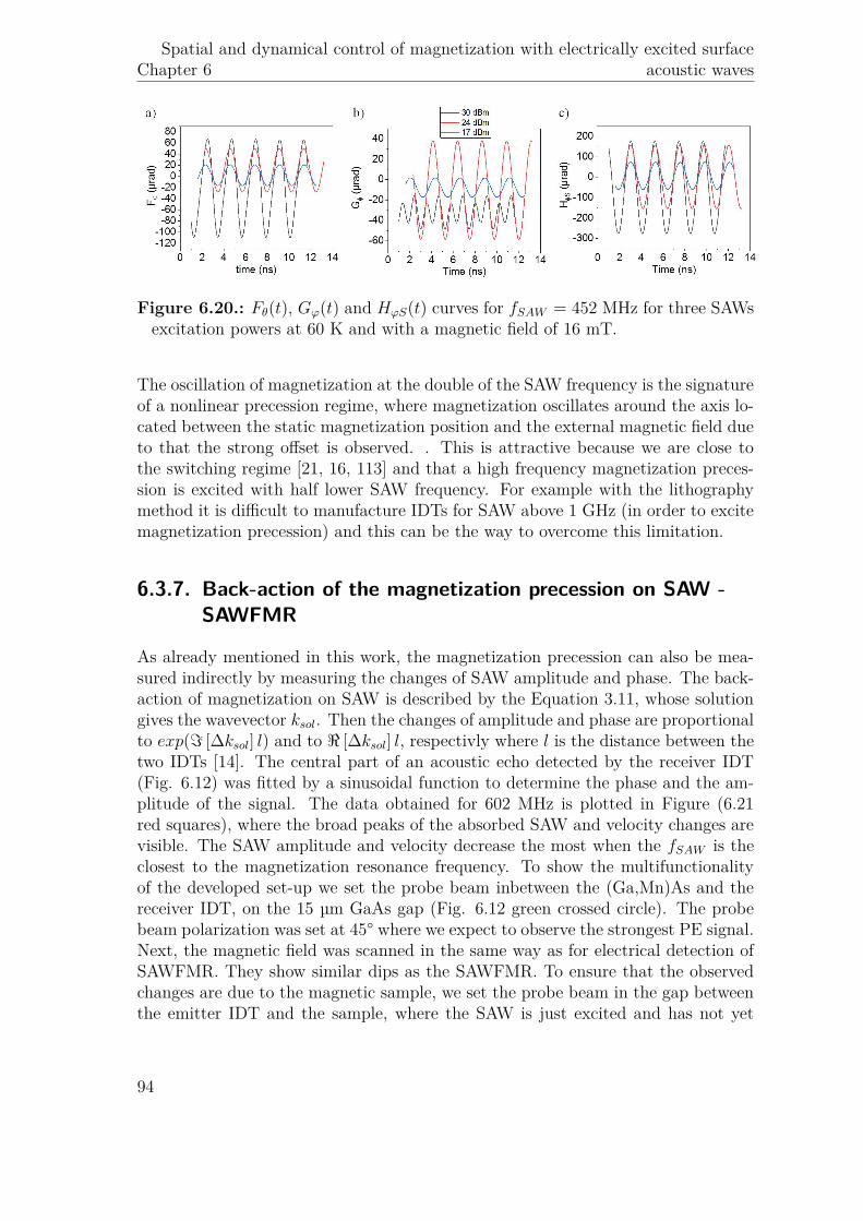
Chapter 6Spatial and dynamical control of magnetization with electrically excited surface
acoustic waves
Figure 6.20.: Fθ(t), Gϕ(t) and HϕS(t) curves for fSAW = 452 MHz for three SAWsexcitation powers at 60 K and with a magnetic field of 16 mT.
The oscillation of magnetization at the double of the SAW frequency is the signatureof a nonlinear precession regime, where magnetization oscillates around the axis lo-cated between the static magnetization position and the external magnetic field dueto that the strong offset is observed. . This is attractive because we are close tothe switching regime [21, 16, 113] and that a high frequency magnetization preces-sion is excited with half lower SAW frequency. For example with the lithographymethod it is difficult to manufacture IDTs for SAW above 1 GHz (in order to excitemagnetization precession) and this can be the way to overcome this limitation.
6.3.7. Back-action of the magnetization precession on SAW -SAWFMR
As already mentioned in this work, the magnetization precession can also be mea-sured indirectly by measuring the changes of SAW amplitude and phase. The back-action of magnetization on SAW is described by the Equation 3.11, whose solutiongives the wavevector ksol. Then the changes of amplitude and phase are proportionalto exp(= [∆ksol] l) and to < [∆ksol] l, respectivly where l is the distance between thetwo IDTs [14]. The central part of an acoustic echo detected by the receiver IDT(Fig. 6.12) was fitted by a sinusoidal function to determine the phase and the am-plitude of the signal. The data obtained for 602 MHz is plotted in Figure (6.21red squares), where the broad peaks of the absorbed SAW and velocity changes arevisible. The SAW amplitude and velocity decrease the most when the fSAW is theclosest to the magnetization resonance frequency. To show the multifunctionalityof the developed set-up we set the probe beam inbetween the (Ga,Mn)As and thereceiver IDT, on the 15 µm GaAs gap (Fig. 6.12 green crossed circle). The probebeam polarization was set at 45° where we expect to observe the strongest PE signal.Next, the magnetic field was scanned in the same way as for electrical detection ofSAWFMR. They show similar dips as the SAWFMR. To ensure that the observedchanges are due to the magnetic sample, we set the probe beam in the gap betweenthe emitter IDT and the sample, where the SAW is just excited and has not yet
94

6.3 Polarization dependence studies
propagated through the magnetic layer. This time, the signal (empty triangles inFig. 6.21) hardly shows any significant variation with the field.
Figure 6.21.: Electrically detected SAWFMR versus optically detected SAWFMR.(a) Amplitude and (b) phase of the electrically and optically measured (in a twoplaces) amplitude and phase variations of the SAWs.
As a result, a maximum attenuation of SAWs was observed for the same field inthe signal detected electrically and optically closer to the receiver IDT. The signaldetected electrically seems to be less noisy, on the grounds that it is faster to measurethe electrical signal and it can be averaged over a few hundred times. In the phasevariation of the optically detected signal we see that it did not return to its originalposition, probably we could not measure it, due to a small drift seen in the presentedfor data detected before the magnetic sample. It is not present in the signal measuredon the receiver IDT, since the whole measurement was at least 10 times shorter.
6.3.7.1. Comparison between the optical detection of magnetization and thestandard SAWFMR
To compare sensitivity and compatibility of the optical detection of magnetizationand electrical SAWFMR techniques we will first consider the data presented in Fig-ure 6.15 (a), since fθ data is the easiest to interpret and compare to the SAWFMR.
95

Chapter 6Spatial and dynamical control of magnetization with electrically excited surface
acoustic waves
Figure 6.22.: Top panels: Field dependence of fθ measured in TRPR for four SAWfrequencies at 60 K. fθ was normalized by the PE effect (baseline of hϕS , not shownhere). Bottom panels: electrically measured variation of the SAW amplitudewith the magnetic field. The excitation powers were the same for optically andelectrically measured signals.
In Fig. 6.22, the top row shows the amplitude of the out-of-plane precession mea-sured optically and the bottom row is the variation of the SAW amplitude detectedelectrically. It is very clear that for SAWFMR measurements, when the amplitudechanges are small (<1%), they are below the detection threshold. This happenedfor the low SAW frequency fSAW= 150 MHz, where we were not able to detect anychanges of the amplitude, while in PMOKE we can clearly observe a sharp peakat the resonance field. As fSAW is higher the SAWFMR dip is more pronounced,but still seems to be more noisy than for optical measurements. With the TRPRmeasurement we are sensitive even to very small changes (a few µrad) because thesignal was detected over a zero background.
6.3.7.2. Temperature dependence- electrical SAWFMR
To confirm the results observed with TRPR for the low (60 K) and high (90 K)temperature (Section 6.3.5), we performed similar studies with SAWFMR. Here wereport the measurement taken for fSAW = 452 MHz at several temperatures forexcitation power 17 dBm.
96

6.3 Polarization dependence studies
Figure 6.23.: The variation of the SAW amplitude versus magnetic field for a sev-eral temperatures. The SAW frequency was equal to 452 MHz and SAWs wereexcited with 17 dBm.
Figure 6.23 reveals similar features as already observed with optical SAWFMR, whenthe temperature is increased the resonance field is shifted to the lower field. More-over, the dip is also bigger (increase of SAW attenuation) for higher temperatureswhich is consistent with fθ.
6.3.8. Spatial mapping of the magnetic and acoustic waves
The final modification of our set-up, which was not discussed in the description ofthe experiment, was introduction of the XYZ piezo stage. This was made in the latespring 2018. The objective was mounted on a remotely movable stage with a rangeof 300 µm in all three directions. By using the stage, we could perform spatiallyresolved maps of SAWs or magnetization precession. In Fig. 6.24 (a), the 150 × 300µm map of propagating SAWs with fSAW = 452 MHz at room temperature (T=291K) is presented. Only part of the image displays the SAW, because the map wastaken at an edge of the excitation transducer, as it is shown in Fig. 6.24 (b), wherethe dashed line rectangle indicates the size and the position of the map.
97
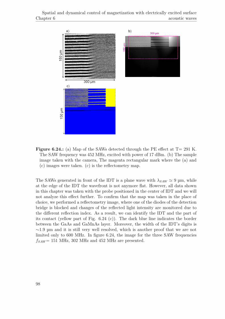
Chapter 6Spatial and dynamical control of magnetization with electrically excited surface
acoustic waves
Figure 6.24.: (a) Map of the SAWs detected through the PE effect at T= 291 K.The SAW frequency was 452 MHz, excited with power of 17 dBm. (b) The sampleimage taken with the camera, The magenta rectangular mark where the (a) and(c) images were taken. (c) is the reflectometry map.
The SAWs generated in front of the IDT is a plane wave with λSAW ' 9 µm, whileat the edge of the IDT the wavefront is not anymore flat. However, all data shownin this chapter was taken with the probe positioned in the center of IDT and we willnot analyze this effect further. To confirm that the map was taken in the place ofchoice, we performed a reflectometry image, where one of the diodes of the detectionbridge is blocked and changes of the reflected light intensity are monitored due tothe different reflection index. As a result, we can identify the IDT and the part ofits contact (yellow part of Fig. 6.24 (c)). The dark blue line indicates the borderbetween the GaAs and GaMnAs layer. Moreover, the width of the IDT’s digits is∼1.9 µm and it is still very well resolved, which is another proof that we are notlimited only to 600 MHz. In figure 6.24, the image for the three SAW frequenciesfSAW= 151 MHz, 302 MHz and 452 MHz are presented.
98

6.3 Polarization dependence studies
Figure 6.25.: Maps taken above TC, using PE effect for three SAWs frequencies:(a) 151 MHz, (b) 302 MHz and (c) 452 MHz. In (d) the image of the sample withthe magenta rectangle that shows were the three maps were taken.
After proving that all used SAW frequencies can be spatially resolved, we performedstudies below TC at T=60 K for fSAW= 453 MHz to image the magnetization preces-sion. However, now the magnetization and strain cannot be as easily distinguishedfrom each other as before, since maps for at least 6 polarizations would need to berecorded and every line of the picture should be analyzed separately. This wouldtake an enormous amount of time if we would like to do it for at least few fieldvalues. Instead, we probed the magnetization with the vertically polarized light(β=0°) where we are not sensitive to PE effect. Nevertheless, the measured signalwas a mixture of the in-plane and out-of-plane magnetization dynamics.
99

Chapter 6Spatial and dynamical control of magnetization with electrically excited surface
acoustic waves
Figure 6.26.: Maps of in-plane and out-of-plane dynamic magnetization compo-nents taken at T=60K with beam polarized at β=0°. The magnetic field for whichthey were taken is indicated above each map. (f) shows the place on the samplewere the maps were detected. (g) The SAWFMR curve, red spots indicate thefields for which maps were taken.
The results are presented in figure 6.26. For a zero magnetic field no magnetizationprecession is detected. Increasing progressively the field, the magnetization preces-sion becomes more visible and at µ0H=20 mT, where we are close to the resonancefield (Fig 6.18 (b) and (g)) the wave is the most intense on the magnetic part of thesample and at 30 mT it disappears again. Furthermore, the wave-like signal wasonly detected at the GaMnAs part in contradiction to the measurement taken withβ=45° where the wave was also detected on the GaAs and underneath IDT. This isanother proof of the magnetic origin of the observed signal.
100
6.4 Perspectives
6.4. Perspectives
As perspectives for the developed set-up we would like to point out the studies ofnonlinear effects, which were just briefly introduced in Section 6.3.6. However, abig number of data have been measured which showed very interesting features,which have not been understood so far. As a perspective, we also need to mentiona time-resolved magnetization switching, which so far was observed only with useof the static MOKE for the excitation with SAWs [16, 180]. The trajectory of themagnetization switching could help us to improve the efficiency of this process. Alsoin this thesis, we did not show the dispersion maps of the magnetic and acousticmodes which are possible to perform in this set-up. Moreover, an interesting exper-iment might be to use the focusing IDT, for which by using the mapping systemwe could image how the magnetization precession changes with the power densityof the SAW.
101


7. Spatial and dynamical control ofmagnetization with opticallyexcited surface acoustic waves
Table of content
7.1 Introduction7.2 Set-up and samples
7.2.1 Set-up7.2.2 Measurement procedure7.2.3 Expected polarization rotation map symmetry7.2.4 Samples (guidelines)
7.3 Results7.3.1 FeGa in zero-field: high precession frequency7.3.2 Nickel in zero-field: low precession frequency7.3.3 FeGa under magnetic field7.3.4 Comparison of dispersion maps for FeGa, Co and Ni7.3.5 Confrontation with the non-magnetic sample
7.4 Conclusions and perspectives
7.1. Introduction
In this chapter we will present results for optically excited SAWs in ferromagneticmetals on transparent substrates. The main challenge of this work was to select asample with suitable magneto-elastic properties and to distinguish the magnetic sig-nal from the acoustic signal. In contrast to SAWs excited with an IDT, the magneti-zation precession was so far not studied with SAWs excited with tightly-focused laserbeam technique. Previously, only the use of unidirectional SAWs excited with theoptical transient grating technique or excited in a patterned samples was reported(Section 4.2.2.2). However, since 2015 several articles reported magnetization pre-cession excitation with BAWs generated in a configuration similar to our (Section4.2.2.1). For both cases a clear evidence of resonance magneto-elastic coupling was
103

Chapter 7Spatial and dynamical control of magnetization with optically excited surface
acoustic waves
shown, confirmed by a strong dependence of the measured signal on the magneticfield.Optical excitation of SAWs has several advantages over the electrical excitation:
• a sample surface being free of any metallic contacts,• excitation of several wavevectors and frequencies,• excitation in 360° directions,• easier synchronization to optical detection,• no need for a piezoelectric substrate.
Hence, the magnetization excitation can be easily studied at various places on thesample surface since preprocessing of samples is not required, which is attractivee.g. for samples with a spatially varying composition of a studied layer. Moreover,with this approach many specimens can be easily examined as it will be shown laterin this chapter. In this project, SAWs are excited with a tightly focused beam (§2.5.1), thus broadband SAWs propagate in 2π directions. This allows us to studythe magnetization precession excited with frequency and wavevector from a widerange, at any angle between the static magnetization and ~kSAW without tuning theexcitation. Only the resonance condition has to be varied via magnetic field to reacha resonance and to increase the efficiency. The magnetization precession and straindynamics are both probed optically. We use polarization rotation measurements asin the Chapter 6 to detect the magnetization dynamics, as well as interferometrymeasurements to measure the out-of-plane displacement.The aim of the study was to determine if a clear signature of SAW-driven magneti-zation precession could be obtained with optically-generated SAWs as was observedfor electrically-generated SAWs.
7.2. Set-up and samples
7.2.1. Set-up
The source of the pump and probe beams was a Ti:Sapphire (MAI-TAI Spectra)laser generating 100 fs long laser pulses of 800 nm wavelength, at a 78.8 GHz repeti-tion rate (Fig. 7.1). At the output, the laser beam was splitted into two beams. Thefrequency of the pump beam was doubled with a BBO crystal. The pump beam wasfocused with a high numerical aperture (NA=0.9) objective to a spot of around 1 µmin diameter (at 1/e2) at one of the interfaces of the sample’s layer. The wavelengthof the excited SAW was directly proportional to the spot diameter [184]. That is whywe have chosen to lower the wavelength of the pump, not of the probe. Additionally,the pump beam was modulated at 0.3 MHz or 1.8 MHz with an acousto-optic mod-ulator (AOM). Before reaching the objective, the probe beam entered a mechanical
104

7.2 Set-up and samples
6×60 cm (12 ns) delay line. Furthermore, since the probe beam was used not onlyto detect the magnetization dynamics by the polarization rotation (PR) but alsothe SAW through interferometric measurements, 50% of the beam was directed toa interferometer reference arm (Michelson interferometer) while the other half wassent to the objective (NA=0.95) and the sample. Then, the reflected beam fromthe sample was detected by the optical bridge. The displacement - Uz was detectedwhen the light reflected from the reference mirror interfered with the one reflectedfrom the sample. Thus, the length of the two paths had to be equal. The PR signalwas detected when the interferometric branch was blocked.
Figure 7.1.: Simplified scheme of the experimental set-up.
The proposed set-up has many advantages:• As it was mentioned, we can perform both PR and interferometry measure-
ments. We detect both signals in a reflection configuration, which is rarein this type of experiments. Most groups detect the polarization rotation intransmission and acoustic signals diffracted on the SAWs in reflection or allacoustic contribution also in transmission ([185, 186]). Nevertheless, the fullreflection set-up was used before by our group to measure the magnetizationprecession induced by picosecond strain and more recently by Yahagi et al. todetect the magnetization precession and SAWs in patterned samples [20, 137].
• The SAW excitation can be either through the substrate or directly on themagnetic layer, which is important as it will be shown later.
• One or both objectives can be mounted on a XYZ piezo stage, which allowsto perform 300 µm × 300 µm XY spatial maps or a 1D scan along a chosenline. If we combine that with the 12 ns delay line, we can take a dispersionmap of either SAWs or spin waves as will be discussed later.
105

Chapter 7Spatial and dynamical control of magnetization with optically excited surface
acoustic waves
However, the use of two objectives with NA>0.9 puts certain constraints on theset-up. The working distance was 1.00+0.35 mm, which means that working at lowtemperature was impossible at least without a specialized cryostat. The limitedspace around the sample impedes the access to it, for example the magnetic fieldcould not be applied as easily. Moreover, the excitation and the detection were oneither side of the sample, therefore the sample’s substrate had to be transparent. Inconclusion, we worked with ferromagnetic metals on different transparent substrates(Section 5.4.2).In contrast to the set-up used for the other project, except for the already mentionedtemperature limitation, another difference was a broadband frequency spectrumexcitation, with a central frequency relying on the focusing. Additionally, with atightly focused laser beam we excited ~kSAW in 2π directions and so the polarizationstudies cannot be used to disentangle the magnetic and photo-elastic (strain - Srrcomponent) contributions as straightforwardly as in the previous chapter.
7.2.2. Measurement procedure
The excitation of magnetization precession with broadband SAWs differs signifi-cantly from the approach presented in the previous chapter, where a few hundredns long acoustic bursts, at a single frequency, forced the magnetization to precessat this frequency. Here, the excitation is broadband. We expect that first mag-netization precesses at SAW frequencies but after the passage of the SAW pulse,magnetization oscillates at its own resonance frequency, for a time defined by thedamping parameter (τd = 1
α2πf ). We expected to observe these features by usingdifferent tools offered by the set-up:
• time scans: the probe can be fixed at a given distance from the excitationpoint and then the optical delay is varied. By performing this measurementin PR and interferometry we expected to observe remarkable differences, suchas different average frequencies and different damping of the oscillations.
• line scans: for this measurements delay line position was set but we could scanfor example a radial line by moving the probe or pump objective. We expectedto see similar results as for the time scans. Moreover, by performing the 1DFFT we obtained the response in the frequency and k space domain for timeand line scans respectively.
• maps: instead of scanning only one line we could scan a large number of lines toobtain a 2D image of acoustic waves or magnetic waves. In the interferometricmap we expected to see a slowness curve, possibly showing the anisotropy ofthe SAW velocity while in the PR map the symmetry breaking defined by anangle between the~kSAW and ~m should appear (see next section).
• dispersion curve: to obtain a dispersion curve either of magnetic or acousticwaves, we needed to take line scans at different optical delays (Fig. 7.2) and
106

7.2 Set-up and samples
process the obtained data with a 2D FFT. From that, we expect to observe adispersion curve of the SAWs and for data taken in PR, part of the dispersioncurve of magnons for places where it crosses the dispersion curve of phonons(Fig. 3.2).
Figure 7.2.: (a) Exemplary line scans measured in the interferometry set-up atdifferent delays between pump and probe (offset for clarity). When enough numberof these scans were taken, they can create the time and space map as it is presentedin (b). Performing the 2D FFT of (b) the dispersion relation in this case of theSAWs can be obtained (c) .
Since the FFT was a frequently used tool to analyze the data in this project, it isworth mentioning that we used a Hanning window.
107

Chapter 7Spatial and dynamical control of magnetization with optically excited surface
acoustic waves
7.2.3. Expected polarization rotation map symmetry
We expect that three axes would break the isotopic symmetry: the probing linearpolarization plane, ~kSAW and the static magnetization. The detected signal shouldhave magnetic and non-magnetic contributions.
7.2.3.1. Magnetic origin
To calculate the signal originating from the magnetization we will start from LLGequation. After T. L. Linnik [79], we neglected the damping and introduced theLL equation in spherical coordinates (Equation 1.16) in the presence of dynamicalstrains:
˙δϕ = γsinΘ0
[∂2f∂Θ2 δΘ + ∂2f
∂Θ∂ϕδϕ+ ∂2f
∂Θ∂SxxδSxx + ∂2f
∂Θ∂SyyδSyy
+ ∂2f∂Θ∂Szz
δSzz + ∂2f∂Θ∂Sxz
δSxz + ∂2f∂Θ∂Syz
δSyz + ∂2f∂Θ∂Sxy
δSxy]
−δΘ̇ = γsinΘ0
[∂2f∂ϕ2 δϕ+ ∂2f
∂ϕ∂ΘδΘ + ∂2f
∂ϕ∂SxxδSxx + ∂2f
∂ϕ∂SyyδSyy
+ ∂2f∂ϕ∂Szz
δSzz + ∂2f∂ϕ∂Sxz
δSxz + ∂2f∂ϕ∂Syz
δSyz + ∂2f∂ϕ∂Sxy
δSxy] (7.1)
Figure 7.3.: (a) Polar coordinates system with the orientation of Ur SAW displac-ment and magnetization. Effect of δϕ̇ in-plane (b) and δΘ̇ out-of plane (c) torques.ψ denotes the orientation of ~kSAW and ϕ of the magnetization.
where f = FMS
is the sum of the magnetocrystalline and magneto-elastic contribu-tions to the free energy F for FeGa [29]:
108

7.2 Set-up and samples
fMCA+MElFeGa = −µ0H[cosΘ cosΘH+sinΘ sinΘH cos(ϕ−ϕH)]+µ0Ms
2 cos2 θ−K2⊥ cos2 θ
+K4‖
4 sin2 2ϕ sin 4θ−K2‖ sin2(ϕ− π
4
)sin2 Θ+B1
[(cos2 ϕSxx + sin2 ϕSyy
)sin2 Θ + cos2 ΘSzz
]
+B2(sin2 Θ sin 2ϕSxy + sin 2Θ sinϕSyz + sin 2Θ cosϕSxz
)(7.2)
one can find the following formulas for the strain induced torques, in the case ofin-plane magnetized samples (Θ0 = π
2 ):
˙δϕ(H, t) = −γ2B2 [cosϕδSxz + sinϕδSyz] + γfΘΘδΘ
− ˙δΘ(H, t) = γB1 sin 2ϕ (−δSxx + δSyy) + 2B2 cos 2ϕδSxy + γfϕϕδϕ(7.3)
For convenience the strains might be rewritten in cylindrical coordinates (Fig. 7.3(a)):
˙δϕ(H, t) = −γ2B2δSrz(t) cos (ϕ− ψ) + γfΘΘδΘ (7.4)
− ˙δΘ(H, t) = γδSrr(t) (−B1 sin 2ϕ cos 2ψ +B2 cos 2ϕ sin 2ψ) + γfϕϕδϕ (7.5)
Here the observation point is located at (r, ψ) in the (x, y) plane (Fig. 7.3 (a)).Equation 7.4 shows that the δSrz strain component acts as an in-plane torque onthe magnetization and can give the symmetry presented in Figure 7.3 (b). Whenthe static magnetization is along ~kSAW (ϕ = ψ), the cosine is equal to 1 and whenit is opposite to it (ϕ = ψ + π) cosine is equal to −1. This gives an opposite phaseacross the epicenter. Moreover, for ϕ − ψ = π
2 or −π2 , no torque is exerted and
we expect not to observe any signal. So we should observe a 2-fold symmetry thatrotates with static ~m position (Fig. 7.3 (b)).Equation 7.5 gives the out-of-plane torque. When B1 = B2 (isotropic magneto-elastic coupling) this torque has a sin 2 (ϕ− ψ) dependence. It depends solely onthe angle between ~m and ~kSAW . It gives a qudrupole-like symmetry for the δΘ andδϕ components (Fig. 7.3 (c)). If B1 6= B2 (cubic symmetry), the symmetry is thesame but is rotated with respect to ~m. For thin Fe80Ga20 samples we have B1= 5MJ/m3 and B2= 3 MJ/m3 [29].
109

Chapter 7Spatial and dynamical control of magnetization with optically excited surface
acoustic waves
7.2.3.2. Non magnetic contribution
Since we observed a clear PE contribution to the PR signal for SAWs generated elec-trically (Chapter 6), it is reasonable to consider the same nonmagnetic contributionin this project. Recalling Equation 5.40, the signal will vary like sin 2β, where β isthe angle between the polarization ~E vector and ~kSAW . As a result, we will get thequadrupole symmetry as it is presented in Figure 7.4.
Figure 7.4.: The calculated photo-elastic contribution in PR signal.
This pattern should rotate, when the incoming polarization is rotated.
7.2.4. Samples (guidelines)
In this project we worked with four different samples. The samples differ from eachother in magnetic layer and substrate. The studied samples were:
• FeGa (88 nm) on STO (0.5µm),• Nickel (100 nm) on glass (0.3 µm),• FeGa (120 nm) on Sapphire (0.5 µm),• Cobalt (100 nm) on Sapphire (0.5 µm).
The FeGa was chosen because of its good magnetostrictive properties. However,the precession frequency was quite high, at least for the FeGa on STO sample (>3GHz at µ0H= 0 mT). It was lower for FeGa on Sapphire (<2 GHz at µ0H= 0 mT)and even lower for Nickel on glass (<1 GHz at µ0H= 0 mT). However, the Rayleighvelocity in glass is small, that is why the peak of the SAW frequency spectrum wasaround 0.8 GHz. The last sample, Cobalt was selected for it is known as a highly
110

7.3 Results
magnetostrictive material and the Sapphire has one of the highest SAW velocitywhich allowed to excite SAWs above 2 GHz.We also used two nonmagnetic samples to confirm the magnetic origin of the mea-sured signals in PR: Aluminium on glass and Titanium on Sapphire.We need to underline, that since the described experimental set-up belongs to Lau-rent Belliard with whom we collaborated on this project, we could work only in shortcampaigns. In total, during 3 years, we had 4 campaigns each lasting from 2 to 4weeks. These campaigns did not yield clear proofs of the magneto-elastic couplingtherefore the results will be presented in chronological order, to show the difficultiesthat we have encountered and how we improved our measurements.
7.3. Results
7.3.1. FeGa in zero-field: high precession frequency
During our first campaign, we studied a magnetically isotropic, epitaxial 88 nmthick FeGa sample on STO substrate in zero field (Section 5.4.2.2). The BBFMRmeasurement shows that the resonance frequency in zero magnetic field was ratherhigh >3GHz (fig. 7.5).
Figure 7.5.: Broadband FMR measurement of FeGa sample on STO. The reso-nance frequency in zero field is difficult to locate but was above 3 GHz.
However, FeGa is known as a good magnetostrictive material and we expected tosee the coupling even if the frequency matching is not optimal [187]. We will startby analyzing the SAWs optically excited on this sample. In Figure 7.6, the interfero-metric map of the generated SAWs is presented. The bright central spot correspondsto the place where the pump laser pulse arrives to excite acoustic waves.
111

Chapter 7Spatial and dynamical control of magnetization with optically excited surface
acoustic waves
Figure 7.6.: FeGa on STO: Interferometry map of optically excited SAWs. TheRayleigh velocity was around υR =4.1km
s.
The signal is isotropic. The inner and outer rings are the SAWs, they are sepa-rated by the distance determined by the laser repetition rate and sound velocity.From the outer ring, we can already say that the propagating SAWs are broadbandand dispersive since we see many fringes. Between the two rings, we can see an-other weaker one, this is the surface skimming longitudinal wave (SSLW). This wavepropagates just below the surface with the velocity of the longitudinal sound wave[188]. Next, we performed a time scan of the SAW. The probe beam was fixed atthe point indicated by the red spot in Fig. 7.6. The result is presented in Figure7.7 (a). First, the acoustic wave with the longer period (lower frequency) arrives,because the velocity for higher frequencies is lower, since they are more sensitive tothe FeGa film. In Fig. 7.7 (b) an FFT of the time profile is presented.
112

7.3 Results
Figure 7.7.: Isotropic FeGa on STO: (a) Time trace of out-of-plane displacementof SAWs. (b) The frequency spectrum from the FFT.
The frequency spectrum was 2 GHz wide at FWHM with the central frequencyaround 1.5 GHz. This frequency depends strongly on the sound velocity in thesubstrate and the spot diameter. After the SAW characterization, we performedKerr studies. The map of the PR measurement is presented in Fig. 7.8 (b). Thered and blue color scale was set for better contrast of the wave phase. The pictureis conspicuously different from the one taken with the interferometry set-up. Thistime, the signal is anisotropic in the ring and in the center. The ring was found atthe same distance from the epicenter as in the interferometry. In two diametricallyopposite parts the ring is clearly weaker than in the other parts. Moreover, by takinga closer look we can see that at the opposite sides of the epicenter, the phase in thering has changed. The epicenter has a two fold symmetry, with the axis crossing thering in the weak part. The obtained symmetry resembles the one expected from thetorque on ϕ (Srz component).
113

Chapter 7Spatial and dynamical control of magnetization with optically excited surface
acoustic waves
Figure 7.8.: Interferometric (a) and PR (b) map taken on FeGa on STO and PRmap for Aluminium sample on glass (c)
Since at that time a magnetic coil was not implemented we performed the same PRmap for a nonmagnetic sample (100 nm on a glass substrate) to test the magneticorigin of the signal (Fig. 7.8 (b)). For Aluminium, the symmetry of the ring wasvery similar, the signal was slightly lower. Although, the signal in the epicenter wasdifferent, it was difficult to analyze it, since the temperature was very high there.Because we observed a similar signal for the Aluminium sample, it was obviously nota good sign and since the FMR frequency was almost out of the excitation frequencyrange for FeGa sample we concluded that the conditions were not fullfilled to observemagneto-elastic coupling. We decided to choose samples with lower FMR frequencyat zero field.
7.3.2. Nickel in zero-field: low precession frequency
From the first campaign, we learned that the frequency coupling might be criticalfor the magnetization precession excited with SAWs. Therefore, we chose a samplewith low FMR frequency in zero magnetic field. This sample was a 100 nm sputteredNickel film on a glass substrate (we have tested also 20 and 300 nm thick Nickelfilms but the results will not be shown here) (Section 5.4.2.1). Since the substratewas different from that for FeGa, the frequency spectrum of the generated SAWswas also slightly different (υR for glass is lower than for STO). In Figure 7.9 (a)and (b) the time profile of the excited SAWs and its FFT are presented. The SAWpeak frequency was clearly lower than before, around 0.8 GHz. To check how itwas located on fFMR(H) curve, we plotted the data extracted from the BBFMRmeasurements (Fig. 5.2 (b) and (c)) in Fig. 7.9 (c).
114

7.3 Results
Figure 7.9.: (a) The time profile of the optically excited SAWs for a 100 nm Nickelsample. (b) The frequency content of the SAWs obtained with FFT. (c) fFMRdependence on magnetic field measured with the BBFMR. The blue bar marksthe frequency band of the SAW from graph (b).
By overlapping the frequency fFMR(H) with the generated SAWs frequency we cansee that for the magnetic field below 20 mT we can expect to see strong magneto-acoustic coupling.For this sample, we have tested two experimental configurations. We will start bypresenting the data for the same configuration as for FeGa on STO where the pumpbeam excites SAWs through the substrate (Fig. 7.10 (a)).
115

Chapter 7Spatial and dynamical control of magnetization with optically excited surface
acoustic waves
Figure 7.10.: (a) Sample orientation for SAW excitation through the substrate.Interferometry and PR maps of Nickel (b). PR map for Aluminium on the glasssubstrate (c).
The results of the interferometric and PR measurements are presented in Fig. 7.10(b) and (c). They are comparable to those obtained for the FeGa sample. Theobserved symmetry in PR maps was tested by applying the magnetic field witha strong permanent magnet along various directions and we observed the samebehavior. Also, we rotated the orientation of the probe polarization, however itdid not influence the symmetry. This rather excludes a purely magnetic origin ofthe signal. The other possibility of the origin of this dipole like symmetry, can bethe deflection of the beam at SAWs as it was proposed in [189]. The probe beam isreflected at a small angle to the normal from the sample surface ridged by the SAWs.If the knife edge is placed in front of the photodetector, some of the k-vectors willbe cut and different intensity will be recorded for light deflected form upward anddownward slope of the surface displacement. This technique was already successfullyapplied to detect gigahertz SAWs [190]. However, we are not sure what could playa role of the knife edge in our experimental set-up.To correlate the signal observed in a ring detected with the interferometry and PR,
116

7.3 Results
we performed two dispersion maps. The dispersion curve of SAWs observed inter-ferometry, showed that the dispersion of SAWs is nearly linear for lower frequenciesbut the velocity (slope) decreases at higher frequency (Fig. 7.11 (a)). It is caused bya stronger sensitivity of higher frequencies to the Nickel layer, which has a quite dif-ferent sound velocity than the substrate. Moreover, we can confirm what we alreadysaw with the 1D FFT (Fig. 7.9 (b)) that the frequency peaks around 0.8 GHz. Thedispersion curve of the signal observed with PR, showed that the maximum intensitywas shifted to around 1.2 GHz. If the PR signal is of magnetic origin, the frequencyshift can be understood as the excitation being the most efficient with the higherfrequency part of the SAWs.
Figure 7.11.: Nickel on glass: Dispersion relations for Interferometry (a) andPMOKE (b) at 0 mT
Figure 7.12 (a) presents the second excitation configuration, where the acousticwaves and magnetic waves are probed through the 200 µm thick glass substrate.The interferometry map now shows some anisotropy (Fig. 7.12 (b)). In the PR mapwe see a different pattern, closer to four-fold symmetry with a change of phase (Fig.7.12 (c)). Moreover, it was now easily visible for the Aluminium layer, which gaveus a clue that this was not magnetic or not purely magnetic signal (Fig. 7.12 (d)).The symmetry is the same as the one predicted for the PE origin. Similar resultswere also reported previously in the literature [191].
117

Chapter 7Spatial and dynamical control of magnetization with optically excited surface
acoustic waves
Figure 7.12.: (a) The configuration of the set-up for detection through the trans-parent substrate. (b) Interferometric and Kerr map for Nickel. The inner ringcorresponds to the Rayleigh acoustic waves and outer ring to SSLW. (c) PR pic-ture for Aluminium.
To understand why the PE effect is higher when we probe through the substrate inthe Figure 7.13 we plotted the amplitude of the SXX strain component versus thesample depth. The strain is present not only in the Nickel layer but also in the glasssubstrate.
118

7.3 Results
Figure 7.13.: The calculated strain SXX amplitude depth dependence for the caseof isotropic Nickel layer on glass (Farnell and Adler’s model for Rayleigh waves[61]).
The strain reaches the highest value at the Nickel layer, however the light travelstwice through the substrate, whose refraction index is modified and the strain isdetected.The difference between the signal in the ring detected with interferometry and PR,was tested with the time traces and 1D FFT. The results of these measurementsfor the Nickel sample are presented in Figure 7.14 (a). The two signals are shiftedin time but have very similar shape. In the frequency range, the signal measuredwith PR peaks at 1.15 GHz, 0.35 GHz higher than in the interferometry (7.14 (b)).There is also a very weak second bump at 4.6 GHz.
119
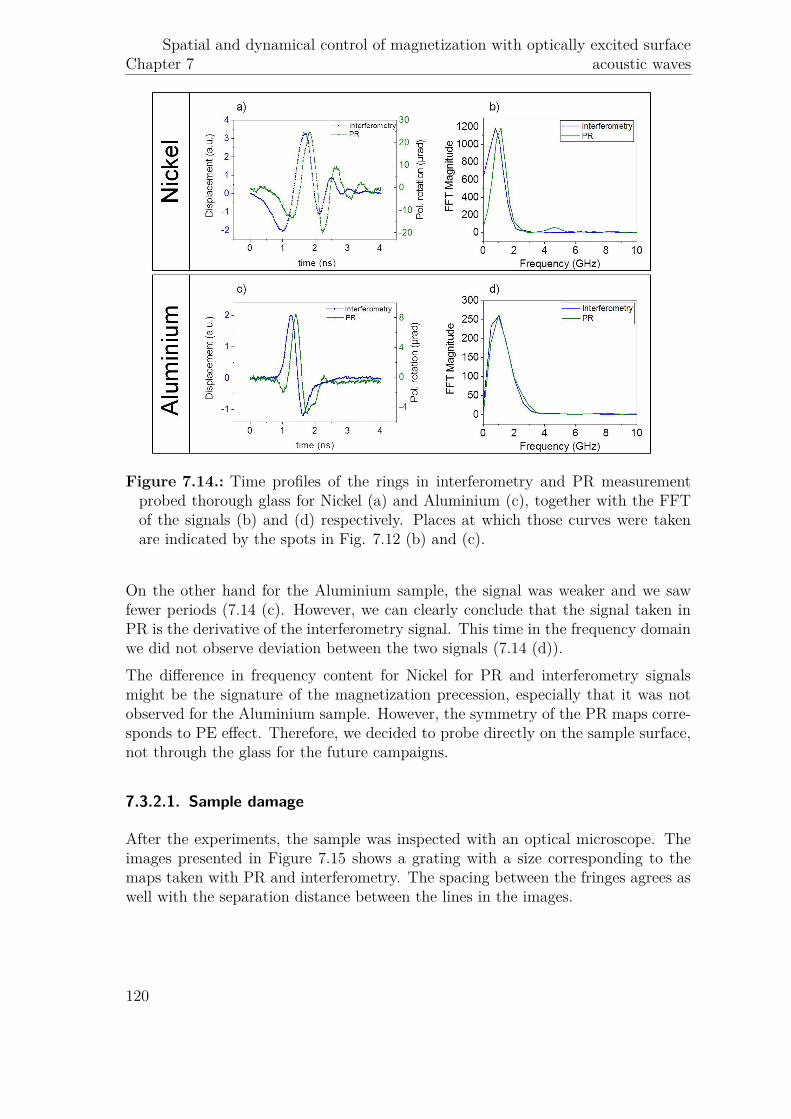
Chapter 7Spatial and dynamical control of magnetization with optically excited surface
acoustic waves
Figure 7.14.: Time profiles of the rings in interferometry and PR measurementprobed thorough glass for Nickel (a) and Aluminium (c), together with the FFTof the signals (b) and (d) respectively. Places at which those curves were takenare indicated by the spots in Fig. 7.12 (b) and (c).
On the other hand for the Aluminium sample, the signal was weaker and we sawfewer periods (7.14 (c). However, we can clearly conclude that the signal taken inPR is the derivative of the interferometry signal. This time in the frequency domainwe did not observe deviation between the two signals (7.14 (d)).The difference in frequency content for Nickel for PR and interferometry signalsmight be the signature of the magnetization precession, especially that it was notobserved for the Aluminium sample. However, the symmetry of the PR maps corre-sponds to PE effect. Therefore, we decided to probe directly on the sample surface,not through the glass for the future campaigns.
7.3.2.1. Sample damage
After the experiments, the sample was inspected with an optical microscope. Theimages presented in Figure 7.15 shows a grating with a size corresponding to themaps taken with PR and interferometry. The spacing between the fringes agrees aswell with the separation distance between the lines in the images.
120

7.3 Results
Figure 7.15.: Microscopy images of the Nickel sample taken in reflection for Nickellayer thickness 100 nm (a), (b) and 20 nm (c).
Since the pump objective was mounted on the piezo stage, we concluded that thegratings were formed due to Nickel ablation by the high fluence pump laser (~3.3mJcm2 ). Moreover, when the penetration depth (δNi ∼= 15 nm [192]) is shorter thanthe sample thickness (100 nm), the efficiency of the ablation can be increased 10times for laser irradiation of the sample from the substrate side as reported before[193, 194]. Because of the evaporation of the metallic layer at the glass/Nickelinterface, the Nickel layer bulges and, when the strain limit is achieved, it lifts-off.These gratings were observed only for 20 nm (Fig. 7.15 (c)) and 100 nm (Fig. 7.15(a) and (b)) Nickel samples but not for the 300 nm and the Aluminium sample.The grating produced might have influenced the magnetic properties of the sample:lower the saturation magnetostriction which was already quite low (λs ∼ 10−6 [195,56]). Thus we had to find a substrate with a better heat conductivity.
7.3.3. FeGa under magnetic field
The final attempt for this project was made in summer 2018. As a sample, thistime we used a FeGa prepared for us in Spain by Rocio Ranchal at UniversidadComplutense de Madrid. Also the following upgrades were made to the experiment:
• A magnetic coil was added to the set-up. To do so, we had to increase thespace between the objectives stages (Fig. 7.16 (a)).
• To obtain higher SAW frequencies and to avoid laser ablation, we used Sap-phire as a substrate. It was chosen for its high sound velocity (Table 2.1) andgood heat conduction. The thermal conductivity for Sapphire at 20°C is 42Wm·K [196], which is much better than for glass: 1 W
m·K [197].• The sample was prepared to have high in-plane magnetic anisotropy [172] in
order to be able to lower the FMR frequency. For samples with distinguishablehard and easy axes, the magnetic field can lower fFMR when it is applied along
121

Chapter 7Spatial and dynamical control of magnetization with optically excited surface
acoustic waves
the hard axis (Fig. 1.6). The FMR frequencies determined from BBFMR areplotted in Fig. 7.16 (b). Data for magnetic field below 20 mT could not bereliably obtained.
• On a selected part of the sample, SiO2 was deposited in order to enhance thePR signal, the thickness of SiO2 was chosen to provide destructive interferenceof the λprobe = 800 nm reflected beam probe [198, 199]. However, the resultwas unsatisfactory, the contrast of static longitudinal MOKE was enhancedonly by 10% and the effect was not visible in PR measurement. Thus we willshow mostly data without the SiO2 layer on the top.
The interferometric map is presented in Fig. 7.16 (c). The ring is slightly anisotropicdue to the hexagonal crystallographic structure of Sapphire substrate. Outside ofthe SAW ring are highly dispersive SSLW waves. They are not as well separated asfor the other samples (Fig. 7.6 and 7.10). Similar features were observed with PR(Fig. 7.16 (d)). The symmetry is the same as for the other samples: 2-fold. Thedifference are oscillations in between the epicenter and the SAW ring. This mightbe long living magnetization oscillations. However, the PR maps under field do notshow significant differences for different field values. In order to check it in a fasterway, we performed time traces.
122

7.3 Results
Figure 7.16.: (a) An image of the experimental set-up with pump and probe objec-tives, the sample located in between the objectives and the magnetic coil behind.(b) Dependence of FMR frequency on the magnetic field obtained in BBFMR.Interferometry (c) and PR (d) maps probing directly on the FeGa side withµ0H= 0mT
The time profile of generated SAWs is presented in Fig. 7.17 (a). First, with thehigher velocity arrives the SSLW (or they might be also a bulk longitudinal wavesince it has the same velocity), which we saw also in the interferometry map. Thebroad frequency content (~3GHz) of SAWs peaks at 2.4 GHz (Fig. 7.17 (b)). Thespectrum covered completely the fFMR(H) curve up to 40 mT (Fig. 7.16 (b)).
123

Chapter 7Spatial and dynamical control of magnetization with optically excited surface
acoustic waves
Figure 7.17.: (a) The time profile of SSLW (black part) and SAW (blue) and FFTof the SAW (b). The SAW frequency spectrum is also overlaid on Fig. 7.16 (b)as a blue bar.
To test if these oscillations are due to a magnetic signal we applied the field alongthe hard axis to tune fFMR. We took a time scan with interferometry and PRmeasurements for 6 field values. For the signal measured in interferometry we didnot expect big changes, however we have noticed that the magnetic field can attractthe probe objective and slightly defocus the beam. Nevertheless, this is mostly thecase for fields above 40 mT. In Figure 7.18 the time traces for interferometry and PRare plotted together for each field on the same chart. Looking at the PR plot for zeromagnetic field (Fig. 7.18 (a)), we can divided the observed signal in four differentregions. First, from 0 to 1.5 ns we observed only the signal originated form theSSLW, which was quite similar for interferometry and for PR. The second regionis from 1.5 to 2.8 ns. It is clearly dominated by the SAW. The frequency of theoscillations is the same for both measurements. Then, from 2.8 to 4 ns we see thatthe frequency for PR and interferometry is not the same anymore. The wave hasa form of the wave packet, probably due to the interference of different frequenciesincluding the SSLW waves that might have not die out and be still present under theSAWs. The most interesting region for us is after 4 ns, where we do not observe theacoustic waves anymore. Thus, we are more sensitive to the pure magnetic signal.This is also the only place where we observed field dependence. If the signal is quiteflat for most of the field values, for µ0H= 20 and 25 mT we observed long livingoscillations at above 3 GHz which are clearly not as well observed for other fieldvalues and interferometry.
124

7.3 Results
Figure 7.18.: FeGa with SiO2 on Sapphire: The time traces measured with PRand interferometry for different field values.
By tuning the magnetic field we expected to observe a change of the frequency inthe PR signal. We went only up to 42 mT, since for higher field values the focusingis lost and the data becomes difficult to compare. In this field range, we shouldbe still well coupled to different frequencies of the SAWs. However, due to the low
125

Chapter 7Spatial and dynamical control of magnetization with optically excited surface
acoustic waves
sensitivity of the detected signal on the magnetic field we can certainly confirm thesmall contribution of the magnetic signal to the PR measurements.
7.3.4. Comparison of dispersion maps for FeGa, Co and Ni
To better resolve the difference between acoustic and magnetic data we recordeddispersion curves for interferometry and PR measurements. Figure 7.19 (a) wastaken in the interferometry set-up for FeGa on Sapphire and it showed the dispersionof the two different waves. The line with the higher slope is the dispersion curve ofSSLW and one with the lower slope corresponds to the SAW. From the slopes wefound the velocities of the two waves: υSSLW = 10.6 km
sand υR = 5.7 km
s. The
dispersion relation for PR is plotted in Figure 7.19 (b) for 20 mT.
Figure 7.19.: Top panel: Dispersion curves measured with (a) interferometry at0 mT, (b) PR at 20 mT and (c) PR at 57 mT for FeGa on Sapphire sample.Time for taking the interferometry maps was 40 min, and 3h for the PR. Longertime for PR is caused by lower intensity. The bottom panel shows the dispersioncurve measured for Cobalt with PR. On the left the frequency projection is shownwhich is a sum of the FFT magnitude in each line. (e) is the maximum magnitudeextracted from (a), (b) and (c) and plotted on the same graph.
126

7.3 Results
As for intereferometry we observed two curves, but this time the SSLW and SAWcurves are not as well separated. Moreover, the highest intensity on the dispersioncurve is localized at higher frequencies, which suggested that the frequency contentof the signal measured in PR is shifted to higher frequencies. The curve with thelower slope was extracted from dispersion map. It is plotted in Fig. 7.19 (e),together with the dispersion curve measured in intereferometry. The two slopes areidentical. This confirms that the signal observed in PR measurement is stronglyrelated to the SAW. Next, to analyze the distribution of intensity in the dispersioncurves in interferometry and PR measurements we projected it on the frequencyaxis, by summing the intensity for each frequency value. This time we can see thedifference, the frequency spectrum of the PR dispersion is narrower (Fig. 7.20 (a)).The low frequency part is missing. However, the variation with the magnetic fieldis rather small, which is presented in Fig. 7.20 (b) where the frequency spectrumtaken at 20 mT is overlaid with the one taken at 57 mT. The position of the centralpeak changes only by 0.2 GHz, while from BBFMR we would expect a much highershift around 5 GHz. Furthermore, the width of the two spectrum is similar. Thesmall difference is for around 3 GHz where another peak appears for the curve takenat 20 mT. This agrees with the time scans observed for the same field (Fig. 7.18(c)), where supplementary oscillations are observe at the frequency associated tothis bump.
127

Chapter 7Spatial and dynamical control of magnetization with optically excited surface
acoustic waves
Figure 7.20.: Dispersion relations projected on the frequency axes for: (a) FeGa(interferometry and PR) at 20 mT, (b) FeGa (PR measured at two field values),(c) Cobalt (interferometry and PR) at 0 mT and (d) Nickel (interferometry andPR taken form Fig. 7.11 (a) and (b)) at 0 mT.
To conclude if this effect was due to the magneto-elastic coupling we performed thesimilar experiment for Cobalt on Sapphire (Section 5.4.2.3) for which results werenot shown so far in this thesis. The fFMR for Co is 1 GHz higher than for FeGa,it is above 2 GHz and we expected to observe frequency spectrum of PR centeredaround higher values. Figure 7.19 (d) shows the dispersion relation measured in PR.The interferometry is not presented because it was very similar to the one obtainedfor FeGa. The SAW velocity is the same as for FeGa since we used the samesubstrate (Fig. 7.19 (e)). In figure 7.20 (c) the projection of the frequency contentin interferometry and PR measurement is plotted. There is a small frequency shiftsimilar to one observed for the Nickel sample (Fig. 7.20 (d)). Moreover, the PRfrequency peaks at 2.4 GHz while for FeGa it was 1.8 GHz, which is consistent withour assumption based on the BBFMR results. However, the frequency of the excitedSAWs is also higher.
128

7.3 Results
7.3.5. Confrontation with the non-magnetic sample
We checked a non-magnetic sample, here a 300 nm Titanium on Sapphire, thesame substrate as for the previously investigated samples: FeGa and Cobalt. Theinterferometry map and PR maps looked very similar to what was obtained before(Fig. 7.21 (a) and (b) respectively). The symmetry of the map observed in PRwas two fold , with a similar orientation of the symmetry axis. Moreover, theshort wavelength fringes are also observed close to the epicenter. To clarify if thedifferences between interferometry and PR signals detected on FeGa also occur againfor this sample, we recorded the time traces (Fig. 7.21 (c)). The frequency of theoscillations detected in the two set-ups was very similar, alike to the other non-magnetic sample, Aluminium on glass (Fig. 7.14 (d)). This is the main indicationthat the observed higher frequency with PR for magnetic samples originates frommagnetization precession.
Figure 7.21.: Ti on sapphire: (a) Interferometry and PR map at 0 mT. (c) Timeprofiles of the oscillations observed in interferometry and PR.
129
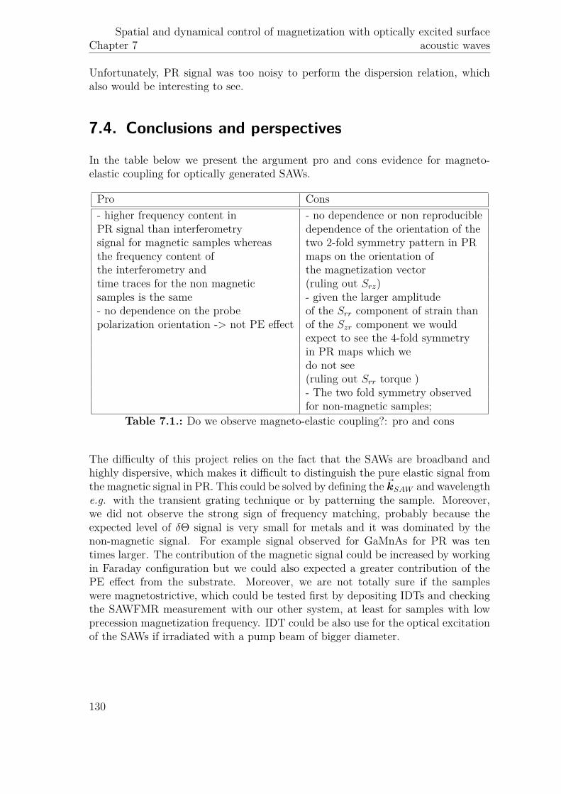
Chapter 7Spatial and dynamical control of magnetization with optically excited surface
acoustic waves
Unfortunately, PR signal was too noisy to perform the dispersion relation, whichalso would be interesting to see.
7.4. Conclusions and perspectives
In the table below we present the argument pro and cons evidence for magneto-elastic coupling for optically generated SAWs.
Pro Cons- higher frequency content in - no dependence or non reproduciblePR signal than interferometry dependence of the orientation of thesignal for magnetic samples whereas two 2-fold symmetry pattern in PRthe frequency content of maps on the orientation ofthe interferometry and the magnetization vectortime traces for the non magnetic (ruling out Srz)samples is the same - given the larger amplitude- no dependence on the probe of the Srr component of strain thanpolarization orientation -> not PE effect of the Szr component we would
expect to see the 4-fold symmetryin PR maps which wedo not see(ruling out Srr torque )- The two fold symmetry observedfor non-magnetic samples;
Table 7.1.: Do we observe magneto-elastic coupling?: pro and cons
The difficulty of this project relies on the fact that the SAWs are broadband andhighly dispersive, which makes it difficult to distinguish the pure elastic signal fromthe magnetic signal in PR. This could be solved by defining the ~kSAW and wavelengthe.g. with the transient grating technique or by patterning the sample. Moreover,we did not observe the strong sign of frequency matching, probably because theexpected level of δΘ signal is very small for metals and it was dominated by thenon-magnetic signal. For example signal observed for GaMnAs for PR was tentimes larger. The contribution of the magnetic signal could be increased by workingin Faraday configuration but we could also expected a greater contribution of thePE effect from the substrate. Moreover, we are not totally sure if the sampleswere magnetostrictive, which could be tested first by depositing IDTs and checkingthe SAWFMR measurement with our other system, at least for samples with lowprecession magnetization frequency. IDT could be also use for the optical excitationof the SAWs if irradiated with a pump beam of bigger diameter.
130

Conclusions and perspectives
In this thesis, we investigated the interaction of surface acoustic waves (SAWs) withmagnetization. The surface acoustic waves were excited electrically and optically.In both cases, the magneto-acoustic signal was detected optically.In the case of SAWs excited electrically with the use of inter digitated transducers(IDTs), it was the first time that the induced magnetization dynamics was detecteddirectly. Before that, the magneto-elastic coupling was detected indirectly as achange of amplitude and phase of the acoustic waves. Here, by locking the phasebetween SAWs and laser pulses, and by studying the polarization rotation in a GaM-nAs sample we detected the in-plane and out-of-plane components of magnetizationdynamics and the in-plane strain component through the PE effect. These studiesshowed that the magnetization precesses at the same frequency as the frequency ofthe acoustic waves in the case of small SAW amplitude. Moreover, the field studiesconfirmed that the magnetization amplitude and SAW absorption peak occur at thesame field, thus evidencing the resonant magneto-elastic coupling by two indepen-dent techniques. The precession efficiency was tested for different SAW excitationpowers, temperatures and SAW frequencies (up to 600 MHz). For a high SAW powerwe observed a nonlinear effect, the precession of magnetization at twice the SAWfrequency. By further investigation of the nonlinear effect: only briefly introducedhere, we believe that new physics could be discovered, which may be especially usefulfor signal processing and magnetization switching.In the second project SAWs were excited optically. This excitation method did notrequire any contacts at the sample surface, which was very convenient. Furthermore,the experimental set-up was very unique since it offered both TR-Kerr detection andinterferometry measurement. A high SAW frequency of around 2.5 GHz for sampleson a Sapphire substrate was obtained. However, the SAW frequency spectrum washighly sensitive to the beam focusing, which made the measurements very difficult toreproduce. Moreover, the excited SAWs were highly dispersive due to the Rayleighvelocity mismatch between the ferromagnetic layer and the substrate. This madethe magnetic signal very difficult to distinguish from the elastic signal. Many ap-proaches were proposed in this work. The most conclusive one was the comparisonof the data obtained for ferromagnetic and nonmagnetic samples. The frequencyspectrum of the polarization rotation signal (potentially containing a magnetic con-tribution) was shifted to higher frequencies with respect to the pure elastic signalfor ferromagnetic layers. However, since the excitation of magnetization precessionwas not very efficient, for future measurements the following solutions should be
131

Conclusions and perspectives
considered:• transmission detection geometry which could increase the contribution of the
magnetic signal, since typically the polarization rotation is a few times higherfor the Faraday configuration than the Kerr configuration. While in thisproject, the Kerr effect and the amplitude of the out-of-plane magnetizationprecession were small comparing to GaMnAs.
• to impose the SAW wavelength with transient grating technique or by pat-terning the sample. By doing this we could concentrate the SAW power in asingle frequency, ensure high reproducibility of the measurements and avoidthe issue of SAW dispersion. The alternative solution for the reduction ofSAW dispersion could be to find a ferromagnetic metal acoustically matchedto a high velocity substrate.
In summary, the two projects showed what a powerful tool for magnetization pre-cession excitation SAWs are. Currently, we were more successful with the electri-cally excited SAWs because they are more narrow band. However, with the opticalmethod we can reach higher frequencies without lithography patterning. GaMnAswas a good material to start with since the resonant magneto-elastic coupling canbe easily obtained and it was already widely studied by our group. We also testedthe magneto-elastic coupling with ferromagnetic metals. However, with the chosenoptical SAW excitation technique it occurred to be a very demanding task and itwill require further work.As a perspective of the study we would like to mention combining our system withmagnonic-phononic crystals, which have been theoretically investigated in the recentyears [200]. In these crystals the propagation properties of magnons and phononscan be designed. With the experimental set-ups used in our work, both acousticand magnetic waves could be imaged in real and reciprocal space which has not yetbeen demonstrated for magnonic-phononic crystals. For example, we could imaginethe realization of a thin 1D periodic structure (for acoustic and magnetic waves)instead of the homogeneous magnetic film. The magnetic-phononic crystals canfold the dispersion curve of magnons and phonons. Thus new crossing points athigh frequencies, where the dispersion of the spin waves is not flat, can be obtained.Hence, the generation of propagating magneto-elastic waves at chosen frequency andwave-vector would be possible.Moreover, with magnonic-phononic crystals we could guide the magnetic and acous-tic waves to separate them from each other and possibly recouple them again, whichis one of the approaches for the realization of logic gates. Also, the band gap of amagnonic-phononic waveguide could be tuned e.g. with the magnetic field or thestatic strain, which would allow to guide a chosen wavelength of the magneto-elasticwaves. Lastly, we would like to mention the usage of the magnonic-phononic crystalsas Bragg mirrors for a resonating cavity of a magnon-phonon laser.
132

A. Expression for the polarizationrotation detected with Lock-in
To find the link between the measured electrical signal and the polarization rotationδβ, let us consider the laser pulse with the Gaussian profile:
I(t) = I0 exp(−t2
a2 ) (A.1)
where a is the pulse duration. Then the intensity reflected from the sample isexpressed by the Dirac delta function: δ(t) = lim
a→01√πa
exp(−t2a2 ), which can be written
as follows:
IR(t) = RI0√πaδ(t) (A.2)
where R is reflection coefficient. The signal was modulated at the pulse selectorfrequency ( fps= fL/N=1/τps) and it is given as:
IR(t) = RI0√πa
∞∑n=0
δ(t− nτps) (A.3)
The intensities of the two orthogonal components of the polarization projected onthe diodes are given as:
IV ert = IR(t) sin2(π4 + δβ
)IHor = IR(t) cos2
(π4 + δβ
) (A.4)
and the difference measured with the bridge:
Idiff (t) = IV ert − IHor = IR(t) sin 2δβ (A.5)
133

Chapter A Expression for the polarization rotation detected with Lock-in
Figure A.1.: (a) Illustration of the polarization rotation and (b) the two modula-tion frequencies: chopper and pulse picker.
We assume that the polarization rotation angle δβ is small with respect to 1, thiswill give ∼ 2δβ rotation. The bridge’s diodes, have their own response describedby the function r(t). Hence the signal observed at the output of the diodes is aconvolution of the reflected intensity and r(t) function:
s = IR(t) ∗ r(t) ∼= 2∫ ∞−∞
IR(u)δβ(u)r (t− u) du (A.6)
The signal from the bridge was detected with the Lock-in amplifier. A lock-inmultiplies the measured signal with the reference signal. As a result, part of thesignal containing the reference frequency is filtered as a DC signal with the low passfilters. The pump signal, in this case acoustic bursts, needs to be modulated at anadditional frequency to provide an effective synchronous detection. In our case themechanical chopper with blades rotating at 541 Hz was placed just before the slowphotodiode (Fig. 6.1). The chopper square modulation signal can be described bythe following function:
fChop(t) = 12 + 2
π
∞∑p=0
sin[(2p+ 1) 2πt
τChop
]2p+ 1 (A.7)
In the case of a polarization rotation angle δβ modulated with the function A.7,Equation A.6 can be rewritten as:
sChop = RI0√πa∫ ∞−∞
∞∑n=0
δ(u− nτps)2δβfChop(u)r (t− u) du (A.8)
134
Expression for the polarization rotation detected with Lock-in
Therefore, the signal detected by lock-in at the chopper frequency, which addition-ally converts it to an rms signal is given as follows:
sChopLock−in = RI02δβ√πa
√2
τChop
×∫ τChop
0
∞∑n=0
r (t− nτps)
12 + 2
π
∞∑p=0
sin[(2p+ 1) 2πt
τChop
]2p+ 1
cos(
2πτChop
t
)dt (A.9)
and the signal detected only by one diode at the chopper frequency
sChop, 1dLock−in(t) = R
2 I0√πa
√2
τps
∫ τChop
0
∞∑n=0
r (t− nτps)
12 + 2
π
∞∑p=0
sin[(2p+ 1) 2πt
τChop
]2p+ 1
cos(
2πτChop
t
)dt
(A.10)
We will need it later to find the polarization rotation. In our experimental set-up thechopper was used to modulate SAWs. Therefore we could not use it to normalize thepolarization rotation. However, because the chopper was triggered externally by anoscillating function generated by the lock-in, we could still use another modulationreference input to detect the signal at a different frequency. Hence we connectedthe reference from the pulse generator (fps), which is the same as reduced laserrepetition rate frequency (fps = fL /N) .The signal detected on a one diode at the pulse selector frequency is given as:
IR(t) = RI0√πa
∞∑n=0
δ(t− nτps) (A.11)
and as before, the signal observed at the output of the diode is a convolution of thereflected intensity and r(t) function:
sDiode(t) = 12IR(t) ∗ r(t) = R
2 I0√πa
∞∑n=0
r(t− nτps) (A.12)
Next, the signal is detected by the lock-in at the pulse selector frequency:
sps, 1dLock−in(t) = R
2 I0√πa
√2
τps
∫ τps
0
∞∑n=0
r(t− nτps) cos(
2πτpst
)dt (A.13)
135

Chapter A Expression for the polarization rotation detected with Lock-in
To find the polarization rotation, the ratio between the differential signal and thesignal measured on one diode at the chopper frequency had to be taken.
sChopLock−in
sChop, 1dLock−in= RI02δβ
√πa
R2 I0√πa
= 4δβ (A.14)
However, because of the reason mentioned above, we used the signal measured at thepulse picker frequency instead of chopper frequency to determine the polarizationrotation. Nevertheless, the pulse selector modulation was very different from thechopper modulation (much shorter window) and additional conversion ratio had tobe added:
δβ = sChopLock−in
4sChop, 1dLock−in= sChopLock−in
4 sChop, 1dLock−insps, 1dLock−in
sps, 1dLock−in
= sChopLock−in
4Rsps, 1dLock−in(A.15)
where the conversion ratio R = sps, 1dLock−insChop, 1dLock−in
was measured with the chopper positionedon the path of the probe beam and it was found to be equal to 1.3 for a bridge gain106.
136
Bibliography
[1] IBM 350 disk storage unit profile: https://www-03.ibm.com/ibm/history/exhibits/storage/storage_350.html.
[2] RAMAC 350 Restoration Web Site: http://www.ed-thelen.org/RAMAC/.[3] Stuart Parkin and See Hun Yang. Memory on the racetrack. Nat. Nanotech-
nol., 10(3):195–198, 2015.[4] M. Collet, O. Gladii, M. Evelt, V. Bessonov, L. Soumah, P. Bortolotti, S. O.
Demokritov, Y. Henry, V. Cros, M. Bailleul, V. E. Demidov, and A. Anane.Spin-wave propagation in ultra-thin YIG based waveguides. Appl. Phys. Lett.,110(9):092408, feb 2017.
[5] A. V. Sadovnikov, C. S. Davies, V. V. Kruglyak, D. V. Romanenko, S. V.Grishin, E. N. Beginin, Y. P. Sharaevskii, and S. A. Nikitov. Spin wavepropagation in a uniformly biased curved magnonic waveguide. Phys. Rev. B,96(6):060401, aug 2017.
[6] T. Fischer, M. Kewenig, D. A. Bozhko, A. A. Serga, I. I. Syvorotka, F. Ciub-otaru, C. Adelmann, B. Hillebrands, and A. V. Chumak. Experimental pro-totype of a spin-wave majority gate. Appl. Phys. Lett., 110(15):152401, apr2017.
[7] Tannous, Charbel and Jacek Gieraltowski. Magnetic Properties: From Tra-ditional to Spintronic. In: Kasap S., Capper P. (eds) Springer Handbook ofElectronic and Photonic Materials. Springer Handbooks. Number 1. SpringerInternational Publishing, Cham, feb 2017.
[8] A. V. Chumak, V. I. Vasyuchka, A. A. Serga, and B. Hillebrands. Magnonspintronics. Nat. Phys., 11(6):453–461, jun 2015.
[9] György Csaba, Ádám Papp, and Wolfgang Porod. Perspectives of using spinwaves for computing and signal processing. Phys. Lett. Sect. A Gen. At. SolidState Phys., 381(17):1471–1476, 2017.
[10] Stephan Breitkreutz-von Gamm, Adam Papp, Eugen Egel, Christian Meier,Cenk Yilmaz, Leonhard Heis, Wolfgang Porod, and Gyorgy Csaba. Designof On-Chip Readout Circuitry for Spin-Wave Devices. IEEE Magn. Lett.,8:3100804, 2017.
[11] Andrii V. Chumak, Alexander A. Serga, and Burkard Hillebrands. Magnontransistor for all-magnon data processing. Nat. Commun., 5(1):4700, dec 2014.
137

Bibliography
[12] T. Fischer, M. Kewenig, D. A. Bozhko, A. A. Serga, I. I. Syvorotka, F. Ciub-otaru, C. Adelmann, B. Hillebrands, and A. V. Chumak. Experimental pro-totype of a spin-wave majority gate. Appl. Phys. Lett., 110(15):152401, apr2017.
[13] L. Dreher, M. Weiler, M. Pernpeintner, H. Huebl, R. Gross, M. S. Brandt, andS. T. B. Goennenwein. Surface acoustic wave driven ferromagnetic resonancein nickel thin films: Theory and experiment. Phys. Rev. B, 86(13):134415, oct2012.
[14] L. Thevenard, C. Gourdon, J. Y. Prieur, H. J. von Bardeleben, S. Vincent,L. Becerra, L. Largeau, and J.-Y. Duquesne. Surface-acoustic-wave-driven fer-romagnetic resonance in (Ga,Mn)(As,P) epilayers. Phys. Rev. B, 90(9):094401,sep 2014.
[15] S. Davis, A. Baruth, and S. Adenwalla. Magnetization dynamics triggered bysurface acoustic waves. Appl. Phys. Lett., 97(23), 2010.
[16] L. Thevenard, I. S. Camara, S. Majrab, M. Bernard, P. Rovillain, A. Lemaître,C. Gourdon, and J.-Y. Duquesne. Precessional magnetization switching by asurface acoustic wave. Phys. Rev. B, 93(13):134430, apr 2016.
[17] J. Dean, M. T. Bryan, J. D. Cooper, A. Virbule, J. E. Cunningham, and T. J.Hayward. A sound idea: Manipulating domain walls in magnetic nanowiresusing surface acoustic waves. Appl. Phys. Lett., 107(14):142405, oct 2015.
[18] Westin Edrington, Uday Singh, Maya Abo Dominguez, James RehwaldtAlexander, Rabindra Nepal, and S. Adenwalla. SAW assisted domain wallmotion in Co/Pt multilayers. Appl. Phys. Lett., 112(5):052402, jan 2018.
[19] Kuntal Roy, Supriyo Bandyopadhyay, and Jayasimha Atulasimha. Hybridspintronics and straintronics: A magnetic technology for ultra low energycomputing and signal processing. Appl. Phys. Lett., 99(6):063108, aug 2011.
[20] L. Thevenard, E. Peronne, C. Gourdon, C. Testelin, M. Cubukcu, E. Charron,S. Vincent, A. Lemaître, and B. Perrin. Effect of picosecond strain pulses onthin layers of the ferromagnetic semiconductor (Ga,Mn)(As,P). Phys. Rev. B,82(10):104422, sep 2010.
[21] L. Thevenard, J.-Y. Duquesne, E. Peronne, H. J. von Bardeleben, H. Jaffres,S. Ruttala, J-M. George, A. Lemaître, and C. Gourdon. Irreversible magne-tization switching using surface acoustic waves. Phys. Rev. B, 87(14):144402,2013.
[22] E. M. Lifshitz L. D. Landau. On the theory of the dispersion of magneticpermeability in ferromagnetic bodies. Phys. Zeitsch. der Sow., (8):153–169,feb 1935.
[23] E. M. Lifshitz L. D. Landau. Statistical physics Part 2: Theory of the con-densed state (Course of theoretical physics; vol. 9). Robert Maxwell, M.C.,1980.
138

Bibliography
[24] T.L. Gilbert. Classics in Magnetics A Phenomenological Theory of Dampingin Ferromagnetic Materials. IEEE Trans. Magn., 40(6):3443–3449, 2004.
[25] P Fulde, M Cardona, and HJ Queisser. Springer series in solid-state sciences.1978.
[26] Stephen Blundell. Magnetism in Condensed Matter. Oxford master Ser. Con-dens. matter Phys., jan 2001.
[27] Kannan M. Krishnan. Fundamentals and Applications of Magnetic Materials.Oxford Univ. Press, 2016.
[28] S. Haghgoo, M. Cubukcu, H. J. von Bardeleben, L. Thevenard, A. Lemaître,and C. Gourdon. Exchange constant and domain wall width in (Ga,Mn)(As,P)films with self-organization of magnetic domains. Phys. Rev. B, 82(4):041301,jul 2010.
[29] Mariana Barturen. Anisotropía magnética y acople magneto-elástico en pelícu-las delgadas de Fe1-xGax crecidas epitaxialmente sobre ZnSe/GaAs(001). PhDthesis, jun 2014.
[30] Robert C. O’Handley. Modern Soft Magnetic Materials, volume 414-415. 2000.[31] E F Silva, M A Corrêa, R D Della Pace, C C Plá Cid, P R Kern, M. Carara,
C. Chesman, O. Alves Santos, R L Rodríguez-Suárez, A. Azevedo, S MRezende, and F. Bohn. Thickness dependence of the magnetic anisotropy anddynamic magnetic response of ferromagnetic NiFe films. J. Phys. D. Appl.Phys., 50(18):185001, may 2017.
[32] P. Němec, E. Rozkotová, N. TesaÅová, F. Trojánek, E. De Ranieri, K. Olejník,J. Zemen, V. Novák, M. Cukr, P. Malý, and T. Jungwirth. Experimentalobservation of the optical spin transfer torque. Nat. Phys., 8(5):411–415, 2012.
[33] Michael Farle. Ferromagnetic resonance of ultrathin metallic layers. ReportsProg. Phys., 61:755–826, 1998.
[34] T. Dietl, H. Ohno, and F. Matsukura. Hole-mediated ferromagnetism in tetra-hedrally coordinated semiconductors. Phys. Rev. B - Condens. Matter Mater.Phys., 63(19), 2001.
[35] J. Stigloher, M. Decker, H. S. Körner, K. Tanabe, T. Moriyama, T. Taniguchi,H. Hata, M. Madami, G. Gubbiotti, K. Kobayashi, T. Ono, and C. H. Back.Snell’s Law for Spin Waves. Phys. Rev. Lett., 117(3):1–5, 2016.
[36] S. Mansfeld, J. Topp, K. Martens, J. N. Toedt, W. Hansen, D. Heitmann, andS. Mendach. Spin wave diffraction and perfect imaging of a grating. Phys.Rev. Lett., 108(4):1–5, 2012.
[37] V. Veerakumar and R. E. Camley. Focusing of spin waves in YIG thin films.IEEE Trans. Magn., 42(10):3318–3320, 2006.
[38] Vladislav E. Demidov, Sergej O. Demokritov, Karsten Rott, Patryk Krzys-teczko, and Guenter Reiss. Mode interference and periodic self-focusing of
139

Bibliography
spin waves in permalloy microstripes. Phys. Rev. B - Condens. Matter Mater.Phys., 77(6):4–9, 2008.
[39] Zhang Zhi-Dong. Spin waves in thin films, superlattices and multilayers. InHandb. Thin Film., chapter Chapter 4, pages 141—-168. Elsevier, 2002.
[40] S O Demokritov, B Hillebrands, and a N Slavin. Brillouin light scatteringstudies of confined spin waves: linear and nonlinear confinement. Phys. Rep.,348(6):441–489, 2001.
[41] B. Lenk, H. Ulrichs, F. Garbs, and M. Münzenberg. The building blocks ofmagnonics. Phys. Rep., 507(4-5):107–136, 2011.
[42] K. Yu Guslienko, S. O. Demokritov, B. Hillebrands, and A. N. Slavin. Effec-tive dipolar boundary conditions for dynamic magnetization in thin magneticstripes. Phys. Rev. B - Condens. Matter Mater. Phys., 66(13):1–4, 2002.
[43] J. Qi, Y. Xu, A. Steigerwald, X. Liu, J. K. Furdyna, I. E. Perakis, and N. H.Tolk. Ultrafast laser-induced coherent spin dynamics in ferromagnetic Ga1-x Mnx As/GaAs structures. Phys. Rev. B - Condens. Matter Mater. Phys.,79(8):1–8, 2009.
[44] Kunihiro Koike, Hironori Asanuma, Satoshi Igarashi, and Shunnsuke Mori.Damping constants of Ni-Fe and Ni-Co alloy thin films. IEEE Trans. Magn.,42(10):2372–2374, 2006.
[45] Christoph Hauser, Tim Richter, Nico Homonnay, Christian Eisenschmidt,Mohammad Qaid, Hakan Deniz, Dietrich Hesse, MacIej Sawicki, Stefan G.Ebbinghaus, and Georg Schmidt. Yttrium Iron Garnet Thin Films with VeryLow Damping Obtained by Recrystallization of Amorphous Material. Sci.Rep., 6(February):1–8, 2016.
[46] Kazuto Yamanoi, Satoshi Yakata, Takashi Kimura, and Takashi Manago. SpinWave Excitation and Propagation Properties in a Permalloy Film. Jpn. J.Appl. Phys., 52(8R):083001, aug 2013.
[47] Sunjae Chung, Anders Eklund, Ezio Iacocca, Seyed Majid Mohseni, Sohrab R.Sani, Lake Bookman, Mark A. Hoefer, Randy K. Dumas, and Johan Åker-man. Magnetic droplet nucleation boundary in orthogonal spin-torque nano-oscillators. Nat. Commun., 7:11209, apr 2016.
[48] S. I. Klselev, J. C. Sankey, I. N. Krivorotov, N. C. Emley, R. J. Schoelkopf,R. A. Buhrman, and D. C. Ralph. Microwave oscillations of a nanomagnetdriven by a spin-polarized current. Nature, 425(6956):380–383, 2003.
[49] N. Locatelli, V. Cros, and J. Grollier. Spin-torque building blocks. Nat. Mater.,13(1):11–20, 2014.
[50] Adrien F. Vincent, Jerome Larroque, Nicolas Locatelli, Nesrine Ben Romd-hane, Olivier Bichler, Christian Gamrat, Wei Sheng Zhao, Jacques-OlivierKlein, Sylvie Galdin-Retailleau, and Damien Querlioz. Spin-Transfer Torque
140

Bibliography
Magnetic Memory as a Stochastic Memristive Synapse for Neuromorphic Sys-tems. IEEE Trans. Biomed. Circuits Syst., 9(2):166–174, apr 2015.
[51] Daniel Royer and Eugène Dieulesaint. Elastic Waves in Solid I: Free andGuided Propagation, 2000.
[52] S. B.Q. Tran, P. Marmottant, and P. Thibault. Fast acoustic tweezers for thetwo-dimensional manipulation of individual particles in microfluidic channels.Appl. Phys. Lett., 101(11), 2012.
[53] Alexey M. Lomonosov, Peter V. Grigoriev, and Peter Hess. Sizing of partiallyclosed surface-breaking microcracks with broadband Rayleigh waves. J. Appl.Phys., 105(8), 2009.
[54] Alexander V. Mamishev, Kishore Sundara-Rajan, Fumin Yang, YanqingDu, and Markus Zahn. Interdigital sensors and transducers. Proc. IEEE,92(5):808–844, 2004.
[55] Y Wang, Z Li, L Qin, M K Chyu, and Q M Wang. Surface acoustic wave flowsensor. 2011 Jt. Conf. IEEE Int. Freq. Control Eur. Freq. Time Forum Proc.,(c):1–4, 2011.
[56] D Sanders. The correlations between mechanical stress and magneticanisotropy in ultra thin film. Reports Prog. Phys., 62(5):809–858, 1999.
[57] Zinoviy Nazarchuk, Valentyn Skalskyi, and Oleh Serhiyenko. Acoustic Emis-sion: Methodology and Application, volume i. Springer, 2017.
[58] B. A. Auld. Acoustic fields and waves in solids, 1973.[59] Arthur A. Oliner. Acoustic surface waves, volume 24. 1978.[60] Ludovic Largeau, Ibrahima Camara, Jean Yves Duquesne, Catherine Gour-
don, Pauline Rovillain, Laura Thevenard, and Bernard Croset. LaboratoryX-ray characterization of a surface acoustic wave on GaAs: The critical roleof instrumental convolution. J. Appl. Crystallogr., 49(6):2073–2081, 2016.
[61] G.W. FARNELL and E.L. ADLER. Elastic Wave Propagation in Thin Layers.In Phys. Acoust. Vol. 9, pages 35–127. Academic Press, 1972.
[62] J D Aussel, A Lebrun, and J C Baboux. Generating Acoustic-Waves by Laser- Theoretical and Experimental-Study of the Emission Source. Ultrasonics,26(5):245–255, 1988.
[63] Daniel Royer and Eugene Dieulesaint. Elastic Waves in Solids II. Generation,Acousto-optic Interaction, Application. Springer-Verlag, 1999.
[64] L. R. F. Rose. Pointâsource representation for laserâgenerated ultrasound. J.Acoust. Soc. Am., 75(3):723–732, 1984.
[65] E. S. Suhubi A. C. Eringen. Elastodynamics, Volum II, Linear theory. Aca-demic Press, 1975.
141

Bibliography
[66] A. M. Aindow, R. J. Dewhurst, and S. B. Palmer. Laser-generation of direc-tional surface acoustic wave pulses in metals. Opt. Commun., 42(2):116–120,1982.
[67] J. Janušonis, C. L. Chang, P. H.M. Van Loosdrecht, and R. I. Tobey. Fre-quency tunable surface magneto elastic waves. Appl. Phys. Lett., 106(18),2015.
[68] D. Royer, E. Dieulesaint, X. Jia, and Y. Shui. Optical generation and detectionof surface acoustic waves on a sphere. Appl. Phys. Lett., 52(9):706–708, feb1988.
[69] Daniel Royer and C Chenu. Experimental and theoretical waveforms ofRayleigh waves generated by a thermoelastic laser line source. Ultrasonics,38(9):891–895, 2000.
[70] M. M. De Lima, F. Alsina, W. Seidel, and P. V. Santos. Focusing of surface-acoustic-wave fields on (100) GaAs surfaces. J. Appl. Phys., 94(12):7848–7855,2003.
[71] Sarah Benchabane, Roland Salut, Olivier Gaiffe, Valérie Soumann, MahmoudAddouche, Vincent Laude, and Abdelkrim Khelif. Surface-Wave Coupling toSingle Phononic Subwavelength Resonators. Phys. Rev. Appl., 8(3):034016,sep 2017.
[72] Kazushi Yamanaka, Noritaka Nakaso, Dongyoun Sim, and Takeshi Fukiura.Principle and application of ball surface acoustic wave (SAW) sensor. Acoust.Sci. Technol., 30(1):2–6, 2009.
[73] L. Sandlund, M. Fahlander, T. Cedell, A. E. Clark, J. B. Restorff, and M.Wun-Fogle. Magnetostriction, elastic moduli, and coupling factors of compositeTerfenol-D. J. Appl. Phys., 75(10):5656–5658, 1994.
[74] N.B. Ekreem, A.G. Olabi, T. Prescott, A. Rafferty, and M.S.J. Hashmi. Anoverview of magnetostriction, its use and methods to measure these properties.J. Mater. Process. Technol., 191(1-3):96–101, aug 2007.
[75] Soshin Chikazumi. Physics of Ferromagnetism. Physics (College. Park. Md).,1(11):655, 1997.
[76] Charles Kittel. Physical Theory of Ferromagnetic Domains. Rev. Mod. Phys.,21(4), 1949.
[77] F; Wooten M.; Batanouny. Symmetry and condensed matter physics. 2008.[78] Hubert Alex and Rudolf Schäfer. Magnetic Domains, volume 40. 1998.[79] T. L. Linnik, A. V. Scherbakov, D. R. Yakovlev, X. Liu, J. K. Furdyna,
and M. Bayer. Theory of magnetization precession induced by a picosec-ond strain pulse in ferromagnetic semiconductor (Ga,Mn)As. Phys. Rev. B,84(21):214432, dec 2011.
142

Bibliography
[80] L.D. Landau E.M. Lifshitz. Theory of Elasticity, 1970.[81] E. W. Lee. Magnetostriction and magnetomechanical effects. Reports Prog.
Phys., 18(1):184–229, 1955.[82] Mingxia Li and Zhihua Feng. Accurate Young’s modulus measurement based
on Rayleigh wave velocity and empirical Poisson’s ratio. Rev. Sci. Instrum.,87(7):075111, jul 2016.
[83] A. K. Ganguly, K. L. Davis, D. C. Webb, and C. Vittoria. Magnetoelasticsurface waves in a magnetic film-piezoelectric substrate configuration. J. Appl.Phys., 47(6):2696–2704, 1976.
[84] I. Feng, M. Tachiki, C. Krischer, and M. Levy. Mechanism for the interactionof surface waves with 200âÅ nickel films. J. Appl. Phys., 53(1):177–193, jan1982.
[85] R. E. Camley. Magnetoelastic waves in a ferromagnetic film on a nonmagneticsubstrate. J. Appl. Phys., 50(8):5272, 1979.
[86] R. Q. Scott and D. L. Mills. Propagation of surface magnetoelastic waves onferromagnetic crystal substrates. Phys. Rev. B, 15(7):3545–3557, 1977.
[87] R. M. Bozorth and H. J. Williams. Effect of small stresses on magnetic prop-erties. Rev. Mod. Phys., 17(1):72–80, 1945.
[88] L. W. McKeehan and P. P. Cioffi. Magnetostriction in Permalloy. Phys. Rev.,28(1):146–157, jul 1926.
[89] P. M. Marcus and F. Jona. Strains in epitaxial films: The general case. Phys.Rev. B, 51(8):5263–5268, 1995.
[90] H Ohno, A Shen, F Matsukura, A Oiwa, A Endo, S Katsumoto, and Y Iye.( Ga , Mn ) As : A new diluted magnetic semiconductor based on GaAs (Ga , Mn ) As : A new diluted magnetic semiconductor based on GaAs. Appl.Phys. Lett., 69:363, 1996.
[91] M. Birowska. Influence of the different strains’ components on the uniax-ial magnetic anisotropy parameters for a (Ga,Mn)As bulk system: A first-principles study. J. Magn. Magn. Mater., 432:396–403, 2017.
[92] J. Wenisch, C. Gould, L. Ebel, J. Storz, K. Pappert, M. J. Schmidt, C. Kumpf,G. Schmidt, K. Brunner, and L. W. Molenkamp. Control of MagneticAnisotropy in (Ga, Mn)As by Lithography-Induced Strain Relaxation. Phys.Rev. Lett., 99(7):077201, aug 2007.
[93] A. Lemaître, A. Miard, L. Travers, O. Mauguin, L. Largeau, C. Gourdon,V. Jeudy, M. Tran, and J. M. George. Strain control of the magnetic anisotropyin (Ga,Mn) (As,P) ferromagnetic semiconductor layers. Appl. Phys. Lett.,93(2), 2008.
143

Bibliography
[94] J. Wunderlich, A. C. Irvine, J. Zemen, V. Holý, A. W. Rushforth, E. DeRanieri, U. Rana, K. Výborný, Jairo Sinova, C. T. Foxon, R. P. Cam-pion, D. A. Williams, B. L. Gallagher, and T. Jungwirth. Local control ofmagnetocrystalline anisotropy in (Ga,Mn)As microdevices: Demonstration incurrent-induced switching. Phys. Rev. B - Condens. Matter Mater. Phys.,76(5):1–8, 2007.
[95] A. W. Rushforth, E. De Ranieri, J. Zemen, J. Wunderlich, K. W. Edmonds,C. S. King, E. Ahmad, R. P. Campion, C. T. Foxon, B. L. Gallagher,K. Výborný, J. Kučera, and T. Jungwirth. Voltage control of magnetocrys-talline anisotropy in ferromagnetic- semiconductor-piezoelectric hybrid struc-tures. Phys. Rev. B - Condens. Matter Mater. Phys., 78(8):1–5, 2008.
[96] E. De Ranieri, A. W. Rushforth, K. Výborný, U. Rana, E. Ahmad, R. P.Campion, C. T. Foxon, B. L. Gallagher, A. C. Irvine, J. Wunderlich, andT. Jungwirth. Lithographically and electrically controlled strain effects onanisotropic magnetoresistance in (Ga,Mn)As. New J. Phys., 10, 2008.
[97] N. A. Pertsev, H. Kohlstedt, and R. Knöchel. Ferromagnetic resonance inepitaxial films: Effects of lattice strains and voltage control via ferroelectricsubstrate. Phys. Rev. B - Condens. Matter Mater. Phys., 84(1):1–7, 2011.
[98] L. Thevenard, I. S. Camara, J.-Y. Prieur, P. Rovillain, A. Lemaître, C. Gour-don, and J.-Y. Duquesne. Strong reduction of the coercivity by a surface acous-tic wave in an out-of-plane magnetized epilayer. Phys. Rev. B, 93(14):140405,apr 2016.
[99] Weiyang Li, Benjamin Buford, Albrecht Jander, and Pallavi Dhagat. Magneticrecording with acoustic waves. Phys. B Condens. Matter, 448:151–154, 2014.
[100] Vimal Sampath, Noel D’Souza, Dhritiman Bhattacharya, Gary M. Atkin-son, Supriyo Bandyopadhyay, and Jayasimha Atulasimha. Acoustic-Wave-Induced Magnetization Switching of Magnetostrictive Nanomagnets fromSingle-Domain to Nonvolatile Vortex States. Nano Lett., 16(9):5681–5687,2016.
[101] H. Bömmel and K. Dransfeld. Excitation of hypersonic waves by ferromagneticresonance. Phys. Rev. Lett., 3(2):83–84, 1959.
[102] P. M. Rowell. Microwave ultrasonics. Br. J. Appl. Phys., 14(2):60–68, 1963.[103] M. Pomerantz. Excitation of Spin-Wave Resonance by Microwave Phonons.
Phys. Rev. Lett., 7(8):312–313, oct 1961.[104] J. P. Parekh and H. L. Bertoni. Magnetoelastic rayleigh-type surface wave on
a tangentially magnetized YIG substrate. Appl. Phys. Lett., 20(9):362–364,1972.
[105] J. P. Parekh and H. L. Bertoni. Magnetoelastic Rayleigh waves on a YIGsubstrate magnetized normal to its surface. J. Appl. Phys., 45(4):1860–1868,1974.
144

Bibliography
[106] J. P. Parekh and H. L. Bertoni. Magnetoelastic Rayleigh waves propagatingalong a tangential bias field on a YIG substrate. J. Appl. Phys., 45(1):434–445,1974.
[107] R.Q. Scott and D.L. Mills. The interaction of Rayleigh waves with ferromag-netic spins; Propagation parallel to the magnetization. Solid State Commun.,18(7):849–852, jan 1976.
[108] R. E. Camley and R. Q. Scott. Surface magnetoelastic waves in the presenceof of exchange interactions and pinning of surface spins. Phys. Rev. B, 17(11),1978.
[109] I. Feng, M. Tachiki, C. Krischer, and M. Levy. Mechanism for the interactionof surface waves with 200âÅ nickel films. J. Appl. Phys., 53(1):177–193, jan1982.
[110] D. Webb, D. Forester, A. Ganguly, and C. Vittoria. Applications of amor-phous magnetic-layers in surface-acoustic-wave devices. IEEE Trans. Magn.,15(6):1410–1415, nov 1979.
[111] Charles Krischer, Ian Feng, Jeffrey B. Block, and Moises Levy. Magnetic-field-dependent attenuation of surface waves by nickel thin films. Appl. Phys. Lett.,29(2):76–77, 1976.
[112] Moises Levy and Hajime Yoshida. Giant attenuation of surface acoustic wavesby ferromagnetic films. J. Magn. Magn. Mater., 35(1-3):139–145, mar 1983.
[113] Piotr Kuszewski, Ibrahima S. Camara, Nicolas Biarrotte, Loic Becerra, Jürgenvon Bardeleben, A. Lemaître, Catherine Gourdon, Jean-Yves Duquesne, andLaura Thevenard. Resonant magneto-acoustic switching: influence of Rayleighwave frequency and wavevector. (001):1–10, 2018.
[114] P. G. Gowtham, T. Moriyama, D. C. Ralph, and R. A. Buhrman. Travelingsurface spin-wave resonance spectroscopy using surface acoustic waves. J.Appl. Phys., 118(23):233910, dec 2015.
[115] V. Polewczyk, K. Dumesnil, D. Lacour, M. Moutaouekkil, H. Mjahed,N. Tiercelin, S. Petit Watelot, H. Mishra, Y. Dusch, S. Hage-Ali, O. Elmazria,F. Montaigne, A. Talbi, O. Bou Matar, and M. Hehn. Unipolar and Bipo-lar High-Magnetic-Field Sensors Based on Surface Acoustic Wave Resonators.Phys. Rev. Appl., 8(2):024001, aug 2017.
[116] N. I. Polzikova, a. O. Raevskii, and a. S. Goremykina. Calculation of thespectral characteristics of an acoustic resonator containing layered multiferroicstructure. J. Commun. Technol. Electron., 58(1):87–94, 2013.
[117] N I Polzikova, I I Pyataikin, S G Alekseev, I M Kotelyanskii, V A Luzanov,and A O Raevskiy. Magnetoelectric bulk acoustic wave resonator for acousticspin pumping. 2016 IEEE Int. Freq. Control Symp., (May):372–373, 2016.
145

Bibliography
[118] N. I. Polzikova, S. G. Alekseev, I. I. Pyataikin, I. M. Kotelyanskii, V. A.Luzanov, and A. P. Orlov. Acoustic spin pumping in magnetoelectric bulkacoustic wave resonator. AIP Adv., 6(5):056306, may 2016.
[119] C. Thomsen, H. T. Grahn, H. J. Maris, and J. Tauc. Surface generation anddetection of phonons by picosecond light pulses. Phys. Rev. B, 34(6):4129–4138, 1986.
[120] O B Wright, T Hyoguchi, and K Kawashima. Laser picosecond acoustic inthin films: effect of elastic boundary conditions on pulse generation. Jpn. J.Appl. Phys., 30(1B):L 131 – L 133, 1991.
[121] A. V. Scherbakov, A. S. Salasyuk, A. V. Akimov, X. Liu, M. Bombeck,C. Brüggemann, D. R. Yakovlev, V. F. Sapega, J. K. Furdyna, and M. Bayer.Coherent magnetization precession in ferromagnetic (Ga,Mn)As induced bypicosecond acoustic pulses. Phys. Rev. Lett., 105(11):1–4, 2010.
[122] L. Thevenard, E. Peronne, C. Gourdon, C. Testelin, M. Cubukcu, E. Charron,S. Vincent, A. Lemaître, and B. Perrin. Effect of picosecond strain pulses onthin layers of the ferromagnetic semiconductor (Ga,Mn)(As,P). Phys. Rev. B- Condens. Matter Mater. Phys., 82(10):1–6, 2010.
[123] M. Bombeck, A. S. Salasyuk, B. A. Glavin, A. V. Scherbakov, C. Brüggemann,D. R. Yakovlev, V. F. Sapega, X. Liu, J. K. Furdyna, A. V. Akimov, andM. Bayer. Excitation of spin waves in ferromagnetic (Ga,Mn)As layers bypicosecond strain pulses. Phys. Rev. B, 85(19):195324, may 2012.
[124] M. Bombeck, J. V. Jäger, A. V. Scherbakov, T. Linnik, D. R. Yakovlev, X. Liu,J. K. Furdyna, A. V. Akimov, and M. Bayer. Magnetization precession inducedby quasitransverse picosecond strain pulses in (311) ferromagnetic (Ga,Mn)As.Phys. Rev. B - Condens. Matter Mater. Phys., 87(6):1–5, 2013.
[125] Ji Wan Kim, Mircea Vomir, and Jean Yves Bigot. Ultrafast magnetoacousticsin nickel. Phys. Rev. Lett., 109(October), 2012.
[126] J. V. Jäger, A. V. Scherbakov, T. L. Linnik, D. R. Yakovlev, M. Wang,P. Wadley, V. Holy, S. A. Cavill, A. V. Akimov, A. W. Rushforth, andM. Bayer. Picosecond inverse magnetostriction in galfenol thin films. Appl.Phys. Lett., 103(3), 2013.
[127] T. L. Linnik, A. V. Scherbakov, D. R. Yakovlev, X. Liu, J. K. Furdyna, andM. Bayer. Theory of magnetization precession induced by a picosecond strainpulse in ferromagnetic semiconductor (Ga,Mn)As. Phys. Rev. B - Condens.Matter Mater. Phys., 84(21):1–11, 2011.
[128] Oleksandr Kovalenko, Thomas Pezeril, and Vasily V. Temnov. New conceptfor magnetization switching by ultrafast acoustic pulses. Phys. Rev. Lett.,110(26):1–5, 2013.
146

Bibliography
[129] Ji Wan Kim and Jean Yves Bigot. Magnetization precession induced by pi-cosecond acoustic pulses in a freestanding film acting as an acoustic cavity.Phys. Rev. B, 95(14):1–6, 2017.
[130] T. Parpiiev, M. Servol, M. Lorenc, I. Chaban, R. Lefort, E. Collet, H. Cailleau,P. Ruello, N. Daro, G. Chastanet, and T. Pezeril. Ultrafast non-thermal laserexcitation of gigahertz longitudinal and shear acoustic waves in spin-crossovermolecular crystals [ Fe ( PM â AzA ) 2 ( NCS ) 2 ]. Appl. Phys. Lett.,111(15):151901, oct 2017.
[131] Yong Xin Yan, Edward B. Gamble, and Keith A. Nelson. Impulsive stimulatedscattering: General importance in femtosecond laser pulse interactions withmatter, and spectroscopic applications. J. Chem. Phys., 83(11):5391–5399,1985.
[132] Naoki Ogawa, Wataru Koshibae, Aron Jonathan Beekman, Naoto Nagaosa,Masashi Kubota, Masashi Kawasaki, and Yoshinori Tokura. Photodriveof magnetic bubbles via magnetoelastic waves. Proc. Natl. Acad. Sci.,112(29):8977–8981, 2015.
[133] Yusuke Hashimoto, Davide Bossini, Tom H. Johansen, Eiji Saitoh, AndreiKirilyuk, and Theo Rasing. Frequency and wavenumber selective excitationof spin waves through coherent energy transfer from elastic waves. Phys. Rev.B, 97(140404):1–5, 2018.
[134] Yusuke Hashimoto, Shunsuke Daimon, Ryo Iguchi, Yasuyuki Oikawa,Ka Shen, Koji Sato, Davide Bossini, Yutaka Tabuchi, Takuya Satoh, BurkardHillebrands, Gerrit E.W. Bauer, Tom H. Johansen, Andrei Kirilyuk, TheoRasing, and Eiji Saitoh. All-optical observation and reconstruction of spinwave dispersion. Nat. Commun., 8(May):1–6, 2017.
[135] Ka Shen and Gerrit E.W. Bauer. Laser-Induced Spatiotemporal Dynamics ofMagnetic Films. Phys. Rev. Lett., 115(19):1–5, 2015.
[136] Ka Shen and Gerrit E. W. Bauer. Theory of spin and lattice wave dynamicsexcited by focused laser pulses. 2:1–7, feb 2018.
[137] Y. Yahagi, B. Harteneck, S. Cabrini, and H. Schmidt. Controlling nanomagnetmagnetization dynamics via magnetoelastic coupling. Phys. Rev. B - Condens.Matter Mater. Phys., 90(14):1–5, 2014.
[138] C. L. Chang, A. M. Lomonosov, J. Janusonis, V. S. Vlasov, V. V. Temnov,and R. I. Tobey. Parametric frequency mixing in a magnetoelastically drivenlinear ferromagnetic-resonance oscillator. Phys. Rev. B, 95(6):1–5, 2017.
[139] K. Hillebrands, B., Ounadjela. Spin Dynamics in Confined Magnetic Struc-tures I, volume 83 of Topics in Applied Physics. Springer Berlin Heidelberg,Berlin, Heidelberg, 2002.
[140] Z. Celinski, K.B. Urquhart, and B. Heinrich. Using ferromagnetic resonance
147

Bibliography
to measure the magnetic moments of ultrathin films. J. Magn. Magn. Mater.,166(1-2):6–26, 1997.
[141] Cheng P. Wen. Coplanar Waveguide: A Surface Strip Transmission LineSuitable for Nonreciprocal Gyromagnetic Device Applications. IEEE Trans.Microw. Theory Tech., 17(12):1087–1090, 1969.
[142] G. Counil, Joo Von Kim, T. Devolder, C. Chappert, K. Shigeto, and Y. Otani.Spin wave contributions to the high-frequency magnetic response of thin filmsobtained with inductive methods. J. Appl. Phys., 95(10):5646–5652, 2004.
[143] Sangita S. Kalarickal, Pavol Krivosik, Mingzhong Wu, Carl E. Patton,Michael L. Schneider, Pavel Kabos, T. J. Silva, and John P. Nibarger. Ferro-magnetic resonance linewidth in metallic thin films: Comparison of measure-ment methods. J. Appl. Phys., 99(9), 2006.
[144] F. Giesen. Magnetization Dynamics of Nanostructured Ferromagnetic Ringsand Rectangular Elements Dissertation. PhD thesis, Univ. Hamburg, Fach-bereich Phys., 2005.
[145] C. Bilzer, T. Devolder, P. Crozat, C. Chappert, S. Cardoso, and P. P. Fre-itas. Vector network analyzer ferromagnetic resonance of thin films on copla-nar waveguides: Comparison of different evaluation methods. J. Appl. Phys.,101(7), 2007.
[146] Simon Foner. Versatile and sensitive vibrating-sample magnetometer. Rev.Sci. Instrum., 30(7):548–557, 1959.
[147] M Faraday. On the magnetization of light and the illumination of magneticlines of force. Philos. Trans. R. Soc. London, 136:1–20, 1846.
[148] E. Hecht. Optics, 2002.[149] Marvin J. Freiser. A Survey of Magnetooptic Effects. IEEE Trans. Magn.,
MAG-4(2):152–161, 1968.[150] Wolfgang Kuch, Rudolf Schäfer, Peter Fischer, and Franz Ulrich Hillebrecht.
Magnetic Microscopy of Layered Structures, volume 57 of Springer Series inSurface Sciences. Springer Berlin Heidelberg, Berlin, Heidelberg, 2015.
[151] J. M. D. Coey. Magnetism and Magnetic Materials. Cambridge UniversityPress, Cambridge, 2010.
[152] T. Kuroiwa, T. Yasuda, F. Matsukura, A. Shen, Y. Ohno, Y. Segawa, andH. Ohno. Faraday rotation of ferromagnetic (Ga, Mn)As. Electron. Lett.,34(2):190, 1998.
[153] A K Zvezdin and V A Kotov. Modern Magnetooptics and MagnetoopticalMaterials. IOP Publishing Ltd, 1997.
[154] K.H.J. Buschow, P.G. van Engen, and R. Jongebreur. Magneto-optical prop-erties of metallic ferromagnetic materials. J. Magn. Magn. Mater., 38(1):1–22,aug 1983.
148

Bibliography
[155] N. TesaÅová, T. Ostatnický, V. Novák, K. Olejník, J. Šubrt, H. Reichlová,C. T. Ellis, A. Mukherjee, J. Lee, G. M. Sipahi, J. Sinova, J. Hamrle, T. Jung-wirth, P. Němec, J. Černe, and K. Výborný. Systematic study of magneticlinear dichroism and birefringence in (Ga,Mn)As. Phys. Rev. B, 89(8):085203,feb 2014.
[156] P. Němec, E. Rozkotová, N. TesaÅová, F. Trojánek, E. De Ranieri, K. Olejník,J. Zemen, V. Novák, M. Cukr, P. Malý, and T. Jungwirth. Experimentalobservation of the optical spin transfer torque. Nat. Phys., 8(5):411–415, 2012.
[157] C. C. Robinson. Longitudinal Kerr Magneto-Optic Effect in Thin Films ofIron, Nickel, and Permalloy*. J. Opt. Soc. Am., 53(6):681, jun 1963.
[158] S Demokritov. Brillouin light scattering studies of confined spin waves: linearand nonlinear confinement. Phys. Rep., 348(6):441–489, jul 2001.
[159] Burkard Hillebrands and Jaroslav Hamrle. Investigation of Spin Waves andSpin Dynamics by Optical Techniques. Handb. Magn. Adv. Magn. Mater.,(December):1–23, 2007.
[160] H. Schultheiss, C. W. Sandweg, B. Obry, S. Hermsdörfer, S. Schäfer, B. Leven,and B. Hillebrands. Dissipation characteristics of quantized spin waves innano-scaled magnetic ring structures. J. Phys. D. Appl. Phys., 41(16):164017,aug 2008.
[161] Moonseok Kim, Sebastien Besner, Antoine Ramier, Sheldon J. J. Kwok, JeesooAn, Giuliano Scarcelli, and Seok Hyun Yun. Shear Brillouin light scatteringmicroscope. Opt. Express, 24(1):319, 2016.
[162] Jean-Charles Beugnot, Sylvie Lebrun, Gilles Pauliat, Hervé Maillotte, VincentLaude, and Thibaut Sylvestre. Brillouin light scattering from surface acousticwaves in a subwavelength-diameter optical fibre. Nat. Commun., 5(1):5242,dec 2014.
[163] Sadao Adachi. Properties of Semiconductor Alloys. John Wiley & Sons, Ltd,Chichester, UK, mar 2009.
[164] H. Ohno, A. Shen, F. Matsukura, A. Oiwa, A. Endo, S. Katsumoto, andY. Iye. (Ga,Mn)As: A new diluted magnetic semiconductor based on GaAs.Appl. Phys. Lett., 69(3):363–365, 1996.
[165] J. Sadowski. GaMnAs: Layers, Wires and Dots. Acta Phys. Pol. A,114(5):1001–1012, nov 2008.
[166] M. Dobrowolska, K. Tivakornsasithorn, X. Liu, J. K. Furdyna, M. Berciu,K. M. Yu, and W. Walukiewicz. Controlling the Curie temperature in(Ga,Mn)As through location of the Fermi level within the impurity band.Nat. Mater., 11(5):444–449, 2012.
[167] L. Chen, S. Yan, P. F. Xu, J. Lu, W. Z. Wang, J. J. Deng, X. Qian, Y. Ji,and J. H. Zhao. Low-temperature magnetotransport behaviors of heavily Mn-
149

Bibliography
doped (Ga,Mn)As films with high ferromagnetic transition temperature. Appl.Phys. Lett., 95(18):2007–2010, 2009.
[168] Kh. Khazen, H. J. von Bardeleben, J. L. Cantin, A. Mauger, L. Chen, and J. H.Zhao. Intrinsically limited critical temperatures of highly doped Ga1âxMnxAsthin films. Phys. Rev. B, 81(23):235201, jun 2010.
[169] A. E. Clark, K. B. Hathaway, M. Wun-Fogle, J. B. Restorff, T. A. Lograsso,V. M. Keppens, G. Petculescu, and R. A. Taylor. Extraordinary magne-toelasticity and lattice softening in bcc Fe-Ga alloys. J. Appl. Phys., 93(103):8621–8623, 2003.
[170] N. Menni M. Hemmous, A. Layadi, A. Guittoum, N. Souami, M. Mebarki.Structure, surface morphology and electrical properties of evaporated Ni thinfilms: Effect of substrates, thickness and Cu underlayer. Thin Solid Films,562:229–238, 2014.
[171] M. Hemmous, A. Layadi, L. Kerkache, N. Tiercelin, V. Preobrazhensky, andP. Pernod. Magnetic Properties of Evaporated Ni Thin Films: Effect of Sub-strates, Thickness, and Cu Underlayer. Metall. Mater. Trans. A Phys. Metall.Mater. Sci., 46(9):4143–4149, 2015.
[172] A. Muñoz-Noval, S. Fin, E. Salas-Colera, D. Bisero, and R. Ranchal. The roleof surface to bulk ratio on the development of magnetic anisotropy in high Gacontent Fe 100-x Ga x thin films. J. Alloys Compd., 745:413–420, may 2018.
[173] Rasmus B. Holländer, Cai Müller, Mathis Lohmann, Babak Mozooni, and Jef-frey McCord. Component selection in time-resolved magneto-optical wide-fieldimaging for the investigation of magnetic microstructures. J. Magn. Magn.Mater., 432:283–290, 2017.
[174] I. S. Camara, B. Croset, L. Largeau, P. Rovillain, L. Thevenard, and J.-Y. Duquesne. Vector network analyzer measurement of the amplitude of anelectrically excited surface acoustic wave and validation by X-ray diffraction.J. Appl. Phys., 121(4):044503, jan 2017.
[175] Wolfgang Maichen. Digital timing measurements: from scopes and probes totiming and jitter. Springer Science & Business Media, 2006.
[176] SITime. Clock Jitter Definitions and Measurement Methods 1. Appl Note,(January):9–10, 2014.
[177] Colin Campbell. Surface Acoustic Wave Devices and Their Signal ProcessingApplications. Academic Press, Inc., 1989.
[178] Florian J.R. Schülein, Eugenio Zallo, Paola Atkinson, Oliver G. Schmidt,Rinaldo Trotta, Armando Rastelli, Achim Wixforth, and Hubert J. Kren-ner. Fourier synthesis of radiofrequency nanomechanical pulses with differentshapes. Nat. Nanotechnol., 10(6):512–516, 2015.
150

Bibliography
[179] Matthias Weiß, Andreas L. Hörner, Eugenio Zallo, Paola Atkinson, ArmandoRastelli, Oliver G. Schmidt, Achim Wixforth, and Hubert J. Krenner. Multi-harmonic Frequency-Chirped Transducers for Surface-Acoustic-Wave Optome-chanics. Phys. Rev. Appl., 9(1):014004, 2018.
[180] Piotr Kuszewski, Ibrahima S. Camara, Nicolas Biarrotte, Loic Becerra, Jür-gen von Bardeleben, W Savero Torres, A. Lemaître, Catherine Gourdon, J-YDuquesne, and Laura Thevenard. Resonant magneto-acoustic switching: in-fluence of Rayleigh wave frequency and wavevector. J. Phys. Condens. Matter,30(24):244003, 2018.
[181] M. Weiler, L. Dreher, C. Heeg, H. Huebl, R. Gross, M. S. Brandt, and S. T. B.Goennenwein. Elastically Driven Ferromagnetic Resonance in Nickel ThinFilms. Phys. Rev. Lett., 106(11):117601, mar 2011.
[182] J. Janušonis, C. L. Chang, P. H. M. van Loosdrecht, and R. I. To-bey. Frequency tunable surface magneto elastic waves. Appl. Phys. Lett.,106(18):181601, may 2015.
[183] A. V. Azovtsev and N. A. Pertsev. Magnetization dynamics and spin pumpinginduced by standing elastic waves. Phys. Rev. B, 94(18):184401, nov 2016.
[184] Zhong-hua Shen, Shu-yi Zhang, and Jian-chun Cheng. Theoretical Study onSurface Acoustic Wave Generated by a Laser Pulse in Solids. In Anal. Sci.Proc. 11th Int. Conf. Photoacoust. Photothermal Phenom., volume 17, pages204–207, 2001.
[185] J. Janušonis, T. Jansma, C. L. Chang, Q. Liu, A. Gatilova, A. M. Lomonosov,V. Shalagatskyi, T. Pezeril, V. V. Temnov, and R. I. Tobey. Transient GratingSpectroscopy in Magnetic Thin Films: Simultaneous Detection of Elastic andMagnetic Dynamics. Sci. Rep., 6(1):29143, sep 2016.
[186] Y. Hashimoto, A. R. Khorsand, M. Savoini, B. Koene, D. Bossini,A. Tsukamoto, A. Itoh, Y. Ohtsuka, K. Aoshima, A. V. Kimel, A. Kir-ilyuk, and Th Rasing. Ultrafast time-resolved magneto-optical imaging ofall-optical switching in GdFeCo with femtosecond time-resolution and a µmspatial-resolution. Rev. Sci. Instrum., 85(6), 2014.
[187] Carolyna Hepburn. Dynamic Interplay between Magnetization and SurfaceAcoustic Waves in Magnetostrictive Fe 1 â x Ga x Thin Films.
[188] A. Abbas, Y. Guillet, J.-M. Rampnoux, P. Rigail, E. Mottay, B. Audoin, andS. Dilhaire. Picosecond time resolved opto-acoustic imaging with 48 MHzfrequency resolution. Opt. Express, 22(7):7831, 2014.
[189] Hiroto Yamazaki, Osamu Matsuda, and Oliver B. Wright. Surface phononimaging through the photoelastic effect. Phys. Status Solidi C Conf.,1(11):2991–2994, 2004.
[190] Julien Higuet, Tony Valier-Brasier, Thomas Dehoux, and Bertrand Audoin.
151

Bibliography
Beam distortion detection and deflectometry measurements of gigahertz sur-face acoustic waves. Rev. Sci. Instrum., 82(11):114905, nov 2011.
[191] Taiki Saito, Osamu Matsuda, Motonobu Tomoda, and Oliver B. Wright. Imag-ing gigahertz surface acoustic waves through the photoelastic effect. J. Opt.Soc. Am. B, 27(12):2632, 2010.
[192] L. Hadley G. Hass. Optical properties of metals. In D. E. Gray, editor, Am.Inst. Phys. Handbook,, chapter 6. McGraw-Hill Book Company, New York,third edition, 1972.
[193] Matthias Domke, Luigi Nobile, Stephan Rapp, Sasia Eiselen, Jürgen Sotrop,Heinz P. Huber, and Michael Schmidt. Understanding thin film laser ablation:The role of the effective penetration depth and the film thickness. Phys.Procedia, 56(C):1007–1014, 2014.
[194] Gerhard Heise, Matthias Domke, Jan Konrad, Sebastian Sarrach, JürgenSotrop, and Heinz P. Huber. Laser lift-off initiated by direct induced ab-lation of different metal thin films with ultra-short laser pulses. J. Phys. D.Appl. Phys., 45(31):315303, aug 2012.
[195] E. Klokholm and J. Aboaf. The saturation magnetostriction of thin poly-crystalline films of iron, cobalt, and nickel. J. Appl. Phys., 53(3):2661–2663,1982.
[196] https://global.kyocera.com/prdct/fc/list/material/.[197] PE Liley RW Powell, CY Ho. Thermal conductivity of selected materials.
National Standard Reference Data Series - National Bureau of Standards,Washington, D. C, 8 edition, 1966.
[198] N. Qureshi, H. Schmidt, and Aaron Hawkins. Cavity-enhanced Kerr effectfor magneto-optic spectroscopy of nanostructures. In Third IEEE Conf. Nan-otechnology. IEEE-NANO 2003., volume 2, pages 175–178. IEEE, 2003.
[199] H. Riahi, L. Thevenard, M.A. Maaref, B. Gallas, A. Lemaître, and C. Gour-don. Optimizing magneto-optical effects in the ferromagnetic semiconductorGaMnAs. J. Magn. Magn. Mater., 395:340–344, dec 2015.
[200] Piotr Graczyk, Jarosław Kłos, and Maciej Krawczyk. Broadband magnetoe-lastic coupling in magnonic-phononic crystals for high-frequency nanoscalespin-wave generation. Phys. Rev. B, 95(10):1–6, 2017.
152