AUTOPILOT DESIGN FOR FIXED WING UAV

AUTOPILOT DESIGN FOR FIXED WING UAV

By

HUDA ELNIEMA ABD-ELRAHMAN ABD-ALLAH

INDEX NO.124107

Supervisor

Prof. Mustafa Nawari

A REPORT SUBMITTED TO

University of Khartoum

In partial fulfillment for the degree of

B.Sc. (HONS) Electrical and Electronics Engineering

(CONTROL AND INSTRUMANTATION ENGINEERING)

Faculty of Engineering

Department of Electrical and Electronic Engineering

October 2017

II

DECLARATION OF ORGINALITY

I declare this report entitled “Autopilot design for fixed wing UAV” is

my own work except as cited in references. The report has been not

accepted for any degree and it is not being submitted currently in

candidature for any degree or other reward.

Signature: ____________________

Name: _______________________

Date: ________________________

III

ACKNOWLEDGEMENT

First and foremost, I would like to thank my supervisor prof. Mustafa Nawari,

who has introduced me to the wonders of control theory, and who has guided me

through this project.

I would like to thank Ustaza Azza Algaily for her useful hints and comments.

She is very dedicated to her work with helping students to advance in their studies.

My gratitude goes to Eng. Mohamed Mahdi from Aviation Researches Centre

(ARC) and Ustaza Dania ALSadig from department of Mechanical Engineering, for

their great help during the journey of this project.

I would also like to thank my advisors Dr. Ahmed ELSayed and Dr. Ahmed

Nasr Eldin Ibrahim for their invaluable guidance and support.

Lastly, I would like to thank my best friend and project partner Mohammed

Abd-Elmoneim, I couldn’t do this without him. I am grateful for all the enjoyable

moments and interesting discussions.

IV

DEDICATION

This thesis is dedicated with love and affection to my Mother for raising me to

believe that anything is possible. Words cannot describe how lucky I’m to have her in

my life. To my family for their continuous support.

Dedicated to Fedaa Awad, Amira Elhadi, Serien Hashim, Hind Hassan,

Hammam Najeeb, Zahraa Najeeb and Eyas Elhashmi who kept me going, when I

wanted to give up. To my best friends and seniors, whose words of encouragement

and push for tenacity ring in my ears.

To coffee, my companion through many a long night of writing.

V

ABSTRACT

Unmanned aerial systems have been widely used for variety of military and

civilian applications over the past few years. Some of these applications require

accurate guidance and control. Consequently, Unmanned Aerial Vehicle (UAV)

guidance and control attracted many researchers in both control theory and aerospace

engineering. Fixed wings, as a particular type of UAV, are considered to have one of

the most efficient aerodynamic structures. The focus of this thesis is on control design

for both lateral and longitudinal for a UAV system. The platform understudy is a fixed

wing developed and modeled by University of Minnesota.

The novel approach suggested in this thesis is to use a successive loop closure

to obtain the gains for the PID controller which is implemented in MATLAB Simulink.

The Software in the Loop Simulation (SIL_Sim) is built by adding actuator and sensor

dynamics that can help prove or test the software.

The performance of the designed controller is compared to the controller of

University of Minnesota. It was found that the performance of the designed controller

is satisfactory in term of time analysis characteristics.

VI

المستخلص

على مدى السنوات القليلة الماضية أصبحت أنظمة الطائرات بدون طيار تستخدم بصورة

بعض هذه التطبيقات تتطلب التوجيه الدقيق و التحكم و المدنية. واسعة فى التطبيقات العسكرية

هتمام أنظار و انتيجة لذلك فإن المركبات الجوية بدون طيار أصبحت محط لهذه الطائرات ؛

من واحدة الطائرات ذات األجنحة الثابتة تعتبر . باحثين فى نظريات التحكم و هندسه الفضاءال

.أكفأ النماذج األيروديناميكية

تركز هذه االطروحة على تصميم أنظمة التحكم لكل من الحركة الجانبية و الطولية

حت الدراسة طائرة ذات جناح ثابت صممت و للمركبات بدون طيار. المنصة أو المنظومة ت

طورت بواسطة جامعة مينيسوتا.

النهج أو الطريقة المقترحة لهذه األطروحة هى استخدام حلقات اإلغالق المتتالية

. ( Simulink)ونفذت باستخدام برنامج الماتالب PIDللحصول على مكاسب من متحكم ال

مع إضافة Software In Loop (SIL)رنامج المحاكاة تم خلق البيئة المطلوبة باستخدام ب

الحساسات و المشغالت الميكانيكية والتي تساعد في إثبات واختبار البرنامج.

قورن أداء المتحكم الذي تم تصميمه بمتحكم جامعة مينيسوتا . ووجد أن أداء المتحكم

لى خصائص تحليل الزمن.المصمم والمقترح في هذه األطروحة قد أعطى نتائج مرضية بناء ع

VII

TABLE OF CONTENTS

DECLARATION OF ORGINALITY .............................................................. II

ACKNOWLEDGEMENT ............................................................................... III

DEDICATION ................................................................................................. IV

ABSTRACT ...................................................................................................... V

VI ............................................................................................................ المستخلص

TABLE OF CONTENTS ............................................................................... VII

LIST OF FIGURES. ......................................................................................... X

LIST OF TABLES. ........................................................................................ XII

LIST OF ABBREVIATIONS ....................................................................... XIII

LIST OF SYMBOLS .................................................................................... XIV

CHAPTER1 INTRODUCTION ..................................................................... 1

1.1 Background .............................................................................................. 1

1.2 Project aim and objectives ....................................................................... 2

CHAPTER2 LITERATURE REVIEW .......................................................... 3

2.1. Coordinate Frames. ........................................................................... 3

2.1.1 The inertial frame Fi. ............................................................................. 4

2.1.2 The vehicle frame Fv. ...................................................................... 4

2.1.3 The vehicle-1 frame Fv1. ................................................................. 4

2.1.4 The vehicle-2 frame Fv2. ................................................................. 5

2.1.5 The body frame Fb. ........................................................................ 6

2.1.6 The stability frame Fs. .................................................................... 7

2.1.7 The wind frame Fw. ........................................................................ 8

2.2 Fixed wing UAV parameters................................................................ 9

2.2.1 Geometric parameters. ................................................................... 9

2.2.2 Basic aerodynamic parameters. ..................................................... 9

2.2.3 Kinematics and dynamics. ............................................................. 10

2.3 Mathematical modeling. ...................................................................... 10

2.3.1. State variables. ............................................................................ 10

2.3.2. Basic aerodynamics. .................................................................... 11

VIII

2.3.3 Forces and moments acting on aircraft. ....................................... 13

2.3.4 Gravitational and thrust forces. .................................................... 13

2.3.5 Kinematic equations. .................................................................... 13

2.3.6 Rigid-body Dynamics. ................................................................. 14

2.3.7 Summary of equations of motion. ................................................ 15

2.3.8 UltraStick25-e. ............................................................................. 17

CHAPTER3 AUTOPILOT DESIGN & SIMULATION.............................. 23

3.1 Introduction. ........................................................................................... 23

3.2 Validation of aircraft model linearization. ......................................... 23

3.2.3 Doublet response of the linear and nonlinear longitudinal model.

24

3.2.4 Doublet response of the linear and nonlinear lateral model. ........ 25

3.3 Automatic Flight Control System (AFCS) ......................................... 26

3.3.1 Successive loops approach. .......................................................... 26

3.3.2 Saturation constraints. .................................................................. 27

3.4 Lateral-directional autopilot. .............................................................. 27

3.4.1 Roll Attitude Loop Design. .......................................................... 28

3.4.2 Course hold loop design. .............................................................. 30

3.4.3 Sideslip hold loop design. ............................................................ 32

3.5 Longitudinal directional controller..................................................... 33

3.5.1 Pitch attitude hold......................................................................... 34

3.5.2 Altitude hold using commanded pitch. ........................................... 36

3.5.3 Airspeed hold using commanded pitch. .......................................... 37

3.5.4 Airspeed hold using throttle. ........................................................ 38

3.6 Controller testing. ............................................................................... 38

3.6.1 Software in loop SIL. ................................................................... 38

3.6.2 Comparison. ................................................................................. 38

CHAPTER4 RESULTS & DISCUSSION .................................................... 40

4.1 Introduction ............................................................................................ 40

4.2 Lateral controller results..................................................................... 40

4.2.1 Direction heading controller......................................................... 42

4.2.2 Sideslip doublet response ............................................................. 43

4.3 Longitudinal controller responses. ..................................................... 45

4.3.1 Pitch Attitude Tracker Simulation Tests. ..................................... 45

IX

4.3.2 Altitude Hold Controller Simulation Tests. ................................. 46

CHAPTER5 CONCLUSION & FUTURE WORK ...................................... 49

5.1 Conclusion ............................................................................................. 49

5.2 Limitations ............................................................................................. 49

5.3 Future Work ........................................................................................... 49

REFERENCES ................................................................................................ 50

APPENDICES ................................................................................................... 1

Appendix A: UAV Nonlinear Simulation Setup ............................................... 1

Appendix B: UAV_NL Model Verification ...................................................... 1

Appendix C: Computing Gains Code ................................................................ 1

Appendix D: Baseline Controller ....................................................................... 1

Appendix E: Heading Controller ....................................................................... 1

Appendix F: UAV Software-in-the-Loop Simulation setup .............................. 1

X

LIST OF FIGURES.

Figure2-1 Inertial frame ..................................................................................... 4

Figure 2-2 Vehicle-1 frame. ............................................................................... 4

Figure 2-3 Vehicle-2 frame. ............................................................................... 5

Figure 2-4 Body frame. ...................................................................................... 6

Figure 2-5 Stability frame. ................................................................................. 7

Figure 2-6 Wind frame....................................................................................... 8

Figure 2-7 Airfoil shape. .................................................................................... 9

Figure 2-8 Wind triangle. ................................................................................. 12

Figure 2-9 UltraStic25-e. ................................................................................. 17

Figure 2-10 Flight scenarios ............................................................................ 19

Figure 3-1 Linear velocity linear response validation. .................................... 23

Figure 3-2 Angular velocity linear response validation. .................................. 24

Figure 3-3 Longitudinal (α, q) doublet response. ............................................ 24

Figure 3-4 Lateral dynamics (β, p, r)response of linear and nonlinear model. 25

Figure 3-5 Open loop system. .......................................................................... 26

Figure 3-6 Successive loops approach. ............................................................ 26

Figure 3-7 Lateral autopilot using successive loops. ....................................... 27

Figure 3-8 Lateral inner loops.......................................................................... 28

Figure 3-9 Roll PD controller. ......................................................................... 29

Figure 3-10 Kiφ using root locus. .................................................................... 29

Figure 3-11 Roll PID controller. ...................................................................... 30

Figure 3-12 Course angle controller design ..................................................... 31

Figure 3-13 Course hold controller. ................................................................. 31

Figure 3-14 Sideslip hold loop. ........................................................................ 32

Figure 3-15 Lateral PID controller. ................................................................. 33

Figure 3-16 Longitudinal controller flight regimes. ........................................ 34

Figure 3-17 Root locus of Pitch tracker. .......................................................... 35

Figure 3-18 Pitch attitude hold controller. ....................................................... 35

Figure 3-19 Altitude hold controller using commanded pitch. ........................ 36

Figure 3-20 Airspeed hold controller using commanded pitch. ...................... 37

Figure 3-21 Airspeed hold controller using throttle. ....................................... 38

XI

Figure 4-1 Doublet response comparison of roll tracker. ................................ 40

Figure 4-2 Doublet response of roll tracker in existance of noise ................... 41

Figure 4-3 Multi step response of the roll tracker. ........................................... 41

Figure 4-4 Doublet signal response of heading angle. ..................................... 42

Figure 4-5 Doublet signal response of heading angle in existence of noise. ... 42

Figure 4-6 Rectangular motion heading command response. .......................... 43

Figure 4-7 Doublet response to β angle ........................................................... 43

Figure 4-8 Doublet signal response of the Φ angle in SIL. ............................. 44

Figure 4-9 Doublet signal response for pitch tracker....................................... 45

Figure 4-10 Doublet signal response of pitch tracker in existence of noise. ... 45

Figure 4-11 Multi steps response for pitch tracker .......................................... 46

Figure 4-12 Step response of altitude hold controller. ..................................... 46

Figure 4-13 Altitude doublet signal response .................................................. 47

Figure 4-14 Altitude doublet signal response with existence of noise. ........... 47

Figure 4-15 Climbing Scenario response. ........................................................ 48

XII

LIST OF TABLES.

Table 2.1 State variables. ................................................................................ 10

Table 2.2 UltraStick25-e specifications. .......................................................... 18

Table 2.3 Trimmed values for UltraStick25-e. ................................................ 20

Table 2.4 Longitudinal poles. .......................................................................... 21

Table 2.5 Lateral poles. .................................................................................... 22

Table 3.1 Errors between linear and nonlinear longitudinal model ................. 25

Table 3.2 Errors between linear and nonlinear lateral model. ......................... 25

Table 3.3 Roll PID controller........................................................................... 30

Table 3.4 Course hold controller. .................................................................... 32

Table 3.5 Sideslip hold controller. ................................................................... 33

Table 3.6 Pitch attitude hold controller............................................................ 36

Table 3.7 Altitude hold controller. ................................................................... 37

Table 3.8 Airspeed hold controller using commanded pitch. .......................... 37

Table 3.9 Airspeed hold controller using throttle. ........................................... 38

Table 3.10 Designed gains and classic gains. .................................................. 39

XIII

LIST OF ABBREVIATIONS

AFCS Automatic Flight Control System.

DOF Degree Of Freedom.

GCS Ground Control Station.

GPS Global Positioning System.

MAV Micro Air Vehicles.

MUAV Mini Unmanned Aerial Vehicle.

NED North East Down.

PID Proportional Integral Differential.

SIL Software In Loop.

SISO Single Input Single Output.

SUAV Small Unmanned Aerial Vehicle.

UAS Unmanned Aircraft Systems.

UAV Unmanned Aerial Vehicle.

XIV

LIST OF SYMBOLS

(ii, ji , ki) Inertial frame axes

(iv, jv, kv) Vehicle frame axes

(ib, jb, kb) Body frame axes

(𝜓, 𝜃, 𝜙) Attitude angles - Euler angles, rad.

α

β

Angle of attack.

Sideslip angle.

𝜒 Course angle.

Γ∗

ρ

Products of the inertia matrix.

Air density.

𝛿𝑎

𝛿𝑒

𝛿𝑟

Aileron deflection.

Elevator deflection.

Rudder deflection.

ζ Damping Coefficient.

𝑎𝜙∗ Constants for transfer function associated with roll dynamics

𝑎𝑥 Acceleration component along x-axis of body frame.

𝑎𝑧 Acceleration component along z-axis of body frame.

B Wing span.

C Mean aerodynamic chord of the wing.

fg Gravity force.

fa Aerodynamic force.

fp Propeller force.

Gp Output vector of accelerometer.

Gpx, Gpy, Gpz Acceleration components of accelerometer.

g Gravitational acceleration (9.81 m/s2) .

J The inertia matrix.

Jx, Jy, Jz, Jxz Elements of the inertia matrix.

kmotor Constant that specifies the efficiency of the motor.

kd_q Feedback damping gain of pitch rate.

kp_θ Proportional gain of pitch angle.

ki_θ Integral gain of pitch angle.

kp_h Proportional gain of altitude.

𝑀∗

State-space coefficients associated with longitudinal dynamics.

XV

m Mass

mb External moment applied to the airframe.

l, m, n The components of mb in Fb.

ma Aerodynamic moment.

mp Propeller moment.

𝑁∗

State-space coefficients associated with lateral dynamics.

𝑝𝑛

The inertial (North) position of the aircraft along ii in Fi.

𝑝𝑒

The inertial (East) position of the aircraft along ji in Fi.

𝑝𝑑

The inertial down position (negative of h (altitude)) of the aircraft

measured along ki in Fi.

𝑝

The roll rate measured along ib in Fb.

𝑞

The pitch rate measured along jb in Fb.

𝑟

The yaw rate measured along kb in Fb.

𝑆𝑝𝑟𝑜𝑝

Area of the propeller.

𝑆𝑌𝑆𝑙𝑎𝑡

State space model associated with lateral dynamics (Alat, Blat, Clat,

Dlat).

𝑆𝑌𝑆𝑙𝑜𝑛𝑔

State space model associated with longitudinal dynamics (Alon,

Blon, Clon, Dlon).

𝑡𝑟

Rise time of step response.

𝑡𝑠

Settling time of step response.

𝑢∗

Trim input.

(𝑢, 𝑣, 𝑤) Velocity components of the airframe projected onto xb-axis.

XVI

𝑉𝑎

Airspeed vector.

𝑉𝑔

Ground speed vector.

𝑉𝑤

Wind speed vector.

𝑥∗ Trim state.

𝑋∗

𝑌∗

𝑍∗


State-space coefficients associated with lateral dynamics.


Chapter 1 Introduction

1

CHAPTER1 INTRODUCTION

High cost and operational limitation of manned aircraft prohibits their use by a

lot of scientific institutions as platforms for research. The use of Unmanned Aerial

Vehicles (UAV) offers a viable alternative. Unmanned Aerial Vehicles (UAVs) become

one of the fastest growing sectors of the world’s aerospace industry.

1.1 Background

There are many different opinions of what an Unmanned Aerial Vehicle (UAV)

is. Many believe that they are only used for military purposes, but this is far from the

truth. The most important definition of an UAV is that it is an aerial vehicle without a

pilot. Without pilot means that the aerial vehicle is flying autonomously. The UAV is

preprogrammed and is supposed to do the operation and come back without human

interference.

Unmanned Aerial Vehicles (UAVs) have many advantages over manned

aircraft: starting from low manufacturing and operational costs of the systems; they

are smaller due to the elimination of the aircrew and related life support systems.

UAVs are capable of flying longer, higher and faster. Furthermore, the development

of small UAVs has been expanded rapidly and used for various purposes such as:

Military applications: reconnaissance surveillance and target acquisition

(RSTA)UAVs surveillance, Meteorology missions, route and landing

reconnaissance support.

Civil Applications:

Scientific Research – In many cases, scientific research necessitates

obtaining data from hazardous or remote locations.

Logistics and Transportation – UAVs can be used to carry and deliver a

variety of payloads.

Disaster and emergency management, industrial applications, etc.

Automatic flight controller is the main building block of UAV , which is known

as autopilot. There are different kinds of autopilots, from the simple ones used in small

private boats to more complex systems used on for instance submarines, oil tankers and

aircrafts [2].

To avoid disasters Autopilot is simulated and tested using MATLAB Simulink

which is a very powerful tool used to estimate the behaviors of systems designed before

implementing them.

UAV can be divided into two categories: Fixed-Wing aircraft & Rotorcraft.

Based on the aircraft role and flight envelope, basic to complex and

sophisticated controllers are used to stabilize the aircraft flight parameters. These

controllers constitute the autopilot system for

Chapter 1 Introduction

2

UAVs. The autopilot systems, most commonly, provide lateral and longitudinal

control through Proportional-Integral-Derivative (PID) controllers. Various techniques

are commonly used to ‘tune’ gains of these controllers.

1.2 Project aim and objectives

This thesis is about small unmanned aircraft which is the class of fixed-wing aircraft

with a wing span between 5 and 10 feet. They are typically designed to operate on the

order of 8 to 20 minutes, with payloads of approximately 10 to 50 pounds.

Autonomy of UAVs requires accurate control systems. Mathematical simulation can be

used to check UAV characteristics, reduce cost, risk and time that is wasted in

experimenting real models.

The main objectives of this thesis are to design a full autonomous controller for a fixed-

wing UAV. The fixed-wing UAV in consideration is UltraStick-25e.

This thesis is organized as follows:

Chapter 2:

includes the modelling of the UAV, its mass-inertia properties. Dynamic model is

based on the 6-DOF equations of motion. Aerodynamic data is used from the

reference [27]. Mass-inertia properties are taken from [27]. UAV model is extracted

in this chapter, is taken from reference [5].

Chapter 3:

The design of autopilot for ULTRA-Stick e25 is introduced using different techniques

such as successive loop closure and root locus.

Chapter 4:

The performance of the designed controller for both lateral and longitudinal parts is

introduced. A variety of setpoints are used to ascertain the attainability of reliable

results. The designed controller is tested against the classical one of university of

Minnesota research team and SIL technique is used to mimic the real aircraft

Chapter 5:

Conclusion and recommendations for future work are presented.

Chapter 2 Literature Review

3

CHAPTER2 LITERATURE REVIEW

In studying unmanned aircraft systems, understanding how different bodies are

oriented relative to each other is very important. In other words, understanding how the

air craft is oriented with respect to earth is the key to determine its behavior. This

chapter describes the various coordinates systems used to express the position and

orientation of the air craft and how to transform between these coordinates. In this

chapter development of a 6-DOF nonlinear model of the ULTRASTICK-25E is

presented. The 6-DOF nonlinear model includes the aerodynamics, atmospheric and

gravity models[1]. The chapter covers linearization of the nonlinear model, decoupling

of airplane dynamics into longitudinal and lateral dynamics, their state space

representations.

2.1. Coordinate Frames.

There are seven major coordinates that describes different aspects of the

aircraft[2]. The transformation from one coordinate frame to another is obtained

through rotation and translation. It is necessary to use several different coordinate

systems for the following reasons:

• Newton’s equations of motion are derived relative to a fixed, inertial reference

frame. However, motion is most easily described in a body-fixed frame.

• Aerodynamic forces and torques act on the aircraft body and are most easily

described in a body-fixed reference frame.

• Sensors like accelerometers and rate gyros measure information with respect

to the body frame. Alternatively, GPS measures position, ground speed, and course

angle with respect to the inertial frame[3].

The inertial frame, vehicle frame, vehicle-1 frame, vehicle-1 frame, body frame,

stability frame, and the wind frame are introduced next. Inertial frame and vehicle frame

are related by translation while other frames are related with rotation. Pitch angle, roll

angle, and yaw angle are the angles which describe the relative orientations of the

vehicle, vehicle-1, vehicle-2, and the body frames. Altitude of the aircraft is determined

by knowing the values of these angles. These angles are commonly known as Euler’s

angles. The rotation angles that define relative orientations between body, stability, and

wind frames are angle of attack and sideslip angle[2][4].


4

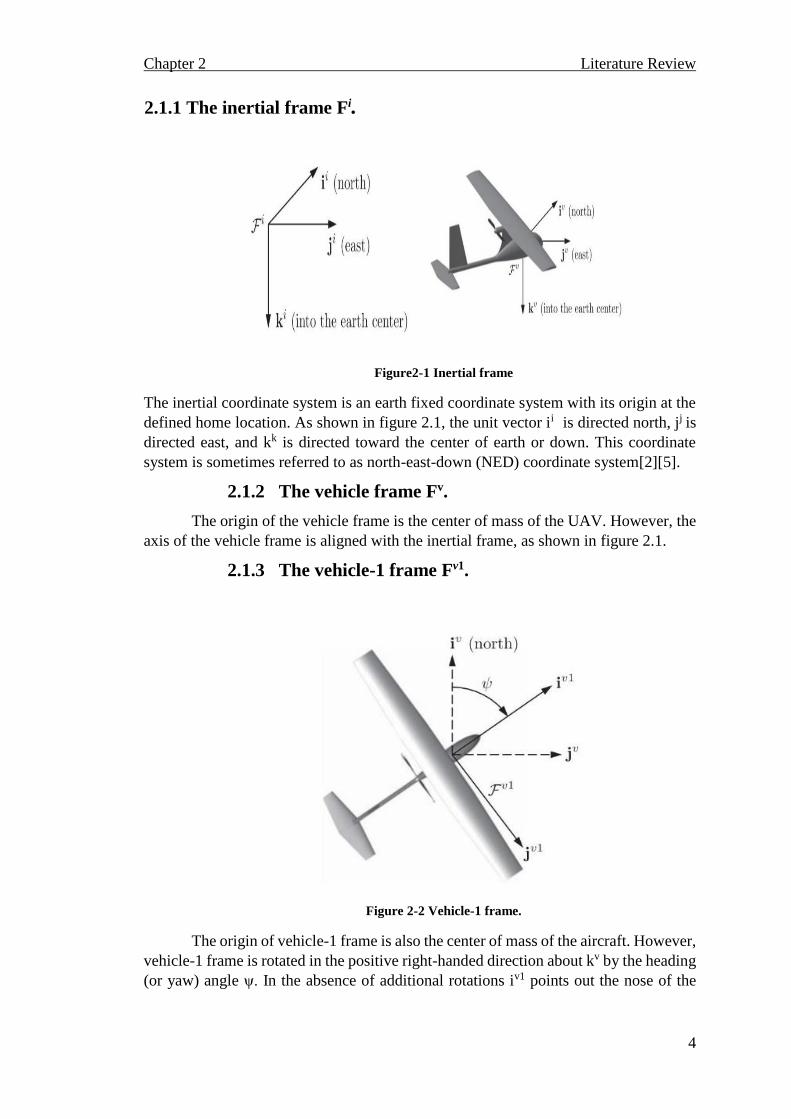
2.1.1 The inertial frame Fi.

Figure2-1 Inertial frame

The inertial coordinate system is an earth fixed coordinate system with its origin at the

defined home location. As shown in figure 2.1, the unit vector ii is directed north, jj is

directed east, and kk is directed toward the center of earth or down. This coordinate

system is sometimes referred to as north-east-down (NED) coordinate system[2][5].

2.1.2 The vehicle frame Fv.

The origin of the vehicle frame is the center of mass of the UAV. However, the

axis of the vehicle frame is aligned with the inertial frame, as shown in figure 2.1.

2.1.3 The vehicle-1 frame Fv1.

Figure 2-2 Vehicle-1 frame.

The origin of vehicle-1 frame is also the center of mass of the aircraft. However,

vehicle-1 frame is rotated in the positive right-handed direction about kv by the heading

(or yaw) angle ψ. In the absence of additional rotations iv1 points out the nose of the


5

airframe, jv1 points out right wing and kv1 is aligned with kv and points into the earth as

in figure 2.2[2].

The transformation from vehicle frame to vehicle-1 frame is given by:

𝑝𝑣1 = 𝑅𝑣1_𝑣𝑝𝑣

Where

𝑅𝑣1_𝑣 = (𝐶𝜓 𝑆𝜓 0

−𝑆𝜓 𝐶𝜓 00 0 1

)

2.1.4 The vehicle-2 frame Fv2.

Figure 2-3 Vehicle-2 frame.

Center of mass of the aircraft is again the origin of vehicle-2 frame. vehicle-2

frame is obtained by rotating vehicle-1 frame in the right-handed side around jv1 axis

by the pitch angle θ. The unit vector iv2 points out the nose of the aircraft, jv2 points out

the right wing, and kv2 points out the belly, as shown in figure 2.3[2].

The transformation from Fv1 to Fv2 is given by:

𝑝𝑣2 = 𝑅𝑣1_𝑣2 𝑝𝑣1

Where

𝑅𝑣1_𝑣2 = (𝐶𝜃 0 −𝑆𝜃0 1 0

𝑆𝜃 0 𝐶𝜃)


6

2.1.5 The body frame Fb.

Figure 2-4 Body frame.

The body frame is obtained by rotating the vehicle-2 frame around the iv2 in the

positive right-handed side by the roll angle φ. There for the unity vector ib points out

the nose of the aircraft, jb points out the right wing and kb out the belly.

The transformation from FV2 to Fb is given by:

𝑝𝑣2 = 𝑅𝑣2_𝑏𝑝𝑣1

Where

𝑅𝑣2_𝑏 = (1 0 00 𝐶φ 𝑆φ0 −𝑆φ 𝐶φ

)

Thus the rotation from vehicle frame to body frame can be obtained directly

using the rotational matrix property[6].

𝑅𝑣2_𝑏𝑅𝑣1_v2𝑅𝑣_𝑣1 = (1 0 00 𝐶φ 𝑆φ0 −𝑆φ 𝐶φ

) (𝐶𝜃 0 −𝑆𝜃0 1 0

𝑆𝜃 0 𝐶𝜃) (

𝐶𝜓 𝑆𝜓 0−𝑆𝜓 𝐶𝜓 0

0 0 1

)

= (

𝐶𝜃𝐶𝜓 𝐶𝜃𝑆𝜓 −𝑆𝜃𝑆𝜑𝑆𝜃𝐶𝜓 − 𝐶𝜑𝑆𝜓 𝑆𝜑𝑆𝜃𝑆𝜓 + 𝐶𝜑𝐶𝜓 𝑆𝜑𝐶𝜃𝐶𝜑𝑆𝜃𝐶𝜓 + 𝑆𝜑𝑆𝜓 𝐶𝜑𝑆𝜃𝑆𝜓 − 𝑆𝜑𝐶𝜓 𝐶𝜑𝐶𝜃

)


7

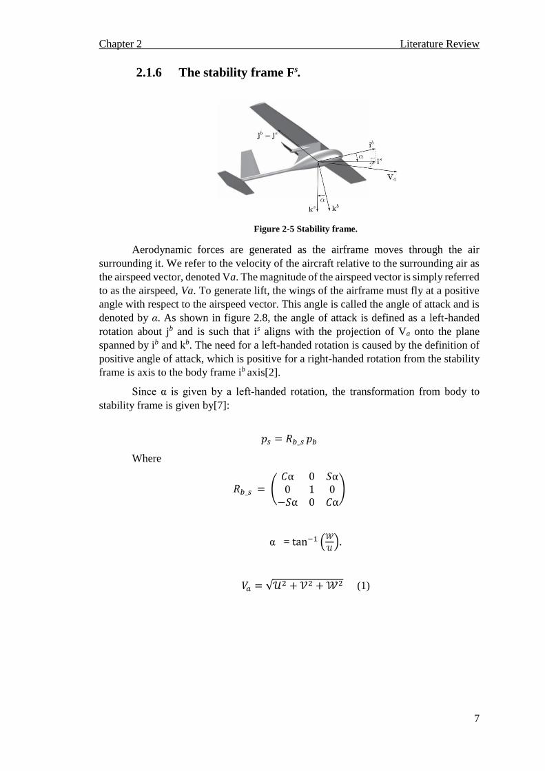
2.1.6 The stability frame Fs.

Figure 2-5 Stability frame.

Aerodynamic forces are generated as the airframe moves through the air

surrounding it. We refer to the velocity of the aircraft relative to the surrounding air as

the airspeed vector, denoted Va. The magnitude of the airspeed vector is simply referred

to as the airspeed, Va. To generate lift, the wings of the airframe must fly at a positive

angle with respect to the airspeed vector. This angle is called the angle of attack and is

denoted by α. As shown in figure 2.8, the angle of attack is defined as a left-handed

rotation about jb and is such that is aligns with the projection of Va onto the plane

spanned by ib and kb. The need for a left-handed rotation is caused by the definition of

positive angle of attack, which is positive for a right-handed rotation from the stability

frame is axis to the body frame ib axis[2].

Since α is given by a left-handed rotation, the transformation from body to

stability frame is given by[7]:

𝑝𝑠 = 𝑅𝑏_𝑠 𝑝𝑏

Where

𝑅𝑏_𝑠 = (𝐶α 0 𝑆α0 1 0

−𝑆α 0 𝐶α)

α = tan−1 (𝒲

𝒰).

𝑉𝑎 = √𝒰2 + 𝒱2 + 𝒲2 (1)


8

2.1.7 The wind frame Fw.

Figure 2-6 Wind frame.

The angle between the velocity vector and the xb-zb plane is called the side-slip

angle and is denoted by β. As shown in figure 2.9, the wind frame is obtained by rotating

the stability frame by a right-handed rotation of β about ks. The unit vector iw is aligned

with the airspeed vector Va[2].

The transformation from stability to wind frame is given by

𝑝𝑤 = 𝑅𝑠_𝑤 𝑝𝑠

Where

𝑅𝑠_𝑤 = (𝐶β 𝑆β 0

−𝑆β 𝐶β 00 0 1

)

The total transformation from the body frame to the wind frame is given by:

𝑅𝑏_𝑤 = 𝑅𝑠_𝑤 𝑅𝑏_𝑠

Where

𝑅𝑏_𝑤 = (CαC β Sβ SαC β

−CαS β Cβ −SαSβ−Sα 0 Cα

)

And

𝛽 = tan−1(𝒱

√𝒰2+𝒲2).


9

2.2 Fixed wing UAV parameters.

This section presents the basic used parameters of the UltraStick-25e (Thor). It

has a conventional fixed-wing airframe with flap, aileron, rudder, and elevator control

surfaces. The maximum deflection of servo actuators equals 25 degrees in each

direction[8].

2.2.1 Geometric parameters.

Figure 2-7 Airfoil shape.

The shape of the airfoil determines its aerodynamic properties, and some of its

geometrical parameters. As shown in figure 2.7.

2.2.2 Basic aerodynamic parameters.

The dynamics of the UAV is decomposed into longitudinal and lateral

dynamics; each of them has some aerodynamic non-dimensional coefficients affect the

stability of the aircraft. These coefficients are parameters in the aerodynamic forces and

moments equations, and influenced by the airfoil design[2].

2.2.2.I Longitudinal Aerodynamic Coefficients

The longitudinal motion acts in the xb-zb plane which is called pitch plane and

affected by the lift force (fL), Drag force (fD), and pitch moment (m). The effectiveness

of these forces and moments are measured by lift coefficient (CL), drag coefficient (CD),

and pitch moment coefficient (Cm). These coefficients influenced by the angle of attack

(α), pitch angular rate (q), and elevator deflection (δe)[9].

2.2.2.II Lateral Aerodynamic Coefficients

The lateral motion which is responsible of the yaw and roll motions. It’s affected

by the side force (fY), yaw moment (𝓃), and roll moment (ℓ). The effectiveness of these

forces and moments are measured by side force coefficient (CY), yaw moment

coefficient (Cn), and roll moment coefficient (Cl). These coefficients influenced by

sideslip angle (𝛽 ), yaw angular rate (r), roll angular rate (p), aileron deflection (𝛿a ) and

rudder deflection (𝛿r )[9].


10

Assuming a flat nonrotating earth surface makes linear approximations for these

coefficients and their derivatives acceptable for modeling purposes and accurate, the

linearization is produced by the first-Taylor approximation, and non-dimensionalize of

the aerodynamic coefficients of the angular rates.

2.2.3 Kinematics and dynamics.

There are three position states and three velocity states associated with the

translational motion of the MAV. Similarly, there are three angular position and three

angular velocity states associated with the rotational motion. The north-east-down

positions of the MAV (Pn, Pe and Pd) are defined relative to the inertial frame. We will

sometimes use h =−Pd to denote the altitude. The linear velocities (u, v and w) and the

angular velocities (p, q and r) of the UAV are defined with respect to the body

frame[8][10].

2.3 Mathematical modeling.

A mathematical model is a representation in mathematical terms of the behavior

of real devices and objects. Since the modeling of devices and phenomena is essential

to both engineering and science, engineers and scientists have very practical reasons

for doing mathematical modeling. Modeling the aircraft allows us to predict the

behavior of the aircraft under certain conditions using simulation; this gives a chance

for avoiding huge losses when system fails, as building an aircraft prototype then testing

its behavior is very expensive especially when talking about fails and errors that could

cause destruction of the prototype[2][11].

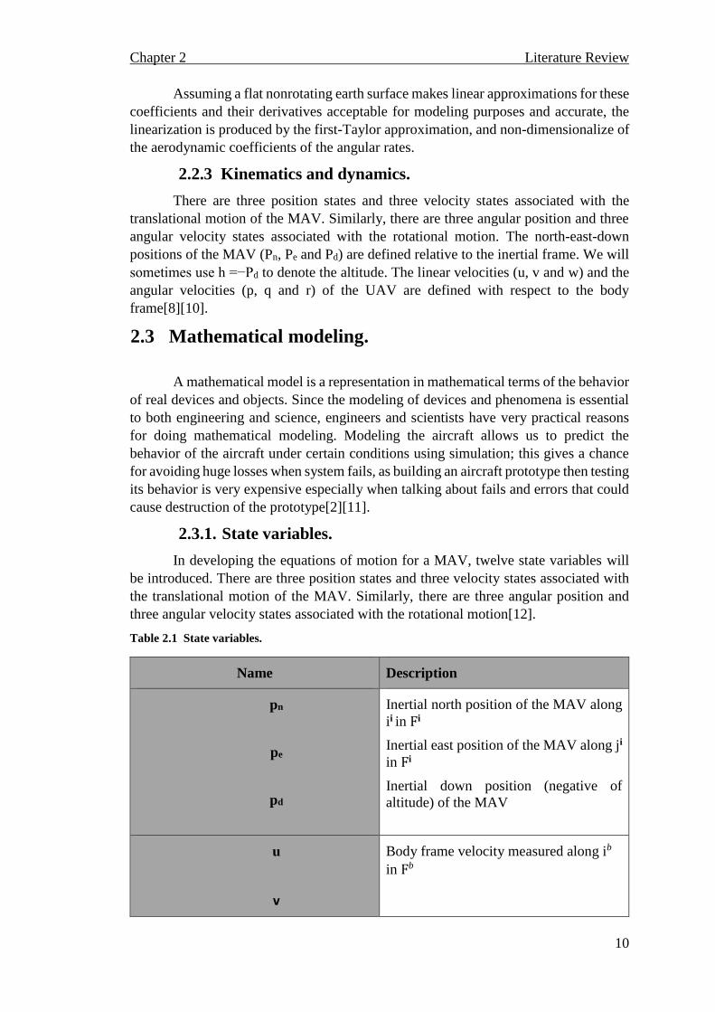
2.3.1. State variables.

In developing the equations of motion for a MAV, twelve state variables will

be introduced. There are three position states and three velocity states associated with

the translational motion of the MAV. Similarly, there are three angular position and

three angular velocity states associated with the rotational motion[12].

Table 2.1 State variables.

Name Description

pn

pe

pd

Inertial north position of the MAV along

ii in Fi

Inertial east position of the MAV along ji

in Fi

Inertial down position (negative of

altitude) of the MAV

u

v

Body frame velocity measured along ib

in Fb


11

w

φ

θ

ψ

Body frame velocity measured along jb

in Fb

Body frame velocity measured along kb

in Fb

Roll angle defined with respect to Fv2v

Pitch angle defined with respect to F 1

Heading (yaw) angle defined with

respect to Fv

p

q

r

Roll rate measured along ib in Fb

Pitch rate measured along jb in Fb

Yaw rate measured along kb in Fb

2.3.2. Basic aerodynamics.

The aerodynamic forces and moments on an aircraft are produced by the relative

motion with respect to the air and depend on the orientation of the aircraft with respect

to the airflow. there are two orientation angles needed to specify the aerodynamic forces

and moments, these angles are the Angle Of Attack (α) and the Sideslip Angle (𝛽), and

are known as the aerodynamic angles. The forces and moments acting on the aircraft

are defined in terms of the aerodynamic angles.

2.3.2.I Airspeed, wind speed, and ground speed.

MAV inertial forces are directly affected with velocities and accelerations

relative to a fixed (inertial) reference frame. Velocity of the airframe relative to the

surrounding air helps determining the aerodynamic forces. In the absence of wind, these

velocities are the same. However, wind is almost always present with MAVs regarding

its light weight and small size. We must carefully distinguish between airspeed,

represented by the velocity with respect to the surrounding air Va, and the ground speed,

represented by the velocity with respect to the inertial frame Vg. These velocities are

related by the expression[2]:

𝑉𝑎 = 𝑉𝑔 − 𝑉𝑤 (2)

Where 𝑉𝑤 is the wind velocity relative to the inertial frame.


12

2.3.2.II The wind triangle.

Figure 2-8 Wind triangle.

Understanding the significant effect of the wind on a MAV is very important

more so than for larger conventional aircraft, where the airspeed is typically much

greater than the wind speed. Introducing the concepts of reference frames, airframe

velocity, wind velocity, and the airspeed vector, gives the ability to discuss some

important definitions relating to the navigation of MAVs. Airspeed is the

vector difference between the groundspeed and the wind speed. On a perfectly still day,

the airspeed is equal to the ground speed. But if the wind is blowing in the same

direction that the aircraft is moving, the airspeed will be less than the groundspeed[2].

The forces and moments acting on the aircraft are defined in terms of the

aerodynamic angles. Dimensionless aerodynamic coefficients and the flight dynamic

pressure as follows[9][13]:

Axial force X = 𝑞SCx = 0.5⍴V2 SCx

Side force Y = 𝑞SCy = 0.5⍴V2SCy

Normal force Z = 𝑞SCz = 0.5⍴V2SC

Rolling force L = 𝑞SCL = 0.5⍴V2SBCL

Pitching force M = 𝑞SCM = 0.5⍴V2𝑐 SCM.

Yawing force N = 𝑞SCN = 0.5⍴V2SBCN.

The aerodynamic coefficients Cx, Cy, Cz, CL, CM, and CN are referred to as

stability derivatives because their values determine the static and dynamic stability of

the MAV.


13

2.3.3 Forces and moments acting on aircraft.

The external forces and moments acting on the aircraft can be re-expressed as

X = FX + GX + XT.

Y = FY + GY + YT.

Z = FZ + GZ + ZT.

L = MX + LT.

M = MY + MT.

N = MZ + NT.

For convenience, X, Y, Z will contain implicitly the propulsive force

components, also L, M, N will contain implicitly the propulsive moment components,

so the nonlinear equations of motions are obtained as follows

X - mg sin θ= m (U + q W - V r).

Y + mg cos θ sin ∅ = m (V + U r - P W).

Z + mg cos θ cos ∅ = m (W + V P - U q).

L = Ixx P - Ixz (r + P q) + (Izz - Iyy) P r.

M= Iyy q + Ixz (p2-r2) + (Ixx - Izz) P r.

N= Izz r - Ixz p + P q (Iyy - Ixx) + Ixz q r.

2.3.4 Gravitational and thrust forces.

The gravitational force acts at the center of gravity of the aircraft. In the aircraft,

the centers of mass and gravity coincide so there is no external moment produced by

gravity about the CG. direct resolution of the vector mg along the coordinate system

axes (x, y, z) yields the following components[14]:

Gx = - mg sinθ.

Gy = mg cosθ sin ∅.

Gz = mg cos ∅ cos θ.

2.3.5 Kinematic equations.

The translational velocity of the MAV is commonly expressed in terms of the

velocity components along each of the axes in a body-fixed coordinate frame. The

components u, v, and w correspond to the inertial velocity of the vehicle projected onto

the ib, jb, and kb axes, respectively. On the other hand, the translational position of the

MAV is usually measured and expressed in an inertial reference frame. Relating the

translational velocity and position requires differentiation and a rotational

transformation.


14

(

𝑝𝑛̇ 𝑝𝑒̇ 𝑝�̇�

) = 𝑅𝑏_𝑣 (𝑢𝑣𝑤

)

(


) = (

𝑐𝜃𝑐𝜓𝑠𝜙𝑠𝜃𝑐𝜓 −𝑐𝜙𝑠𝜓𝑐𝜙𝑠𝜃𝑐𝜓 𝑠𝜙𝑠𝜓

𝑐𝜃𝑠𝜓𝑠𝜙𝑠𝜃𝑠𝜓 𝑐𝜙𝑐𝜓𝑐𝜙𝑠𝜃𝑠𝜓 −𝑠𝜙𝑐𝜓

−𝑠𝜃 𝑠𝜙𝑐𝜃 𝑐𝜙𝑐𝜃

) (𝑢𝑣𝑤

)

This is a kinematic relation in that it relates the derivative of position to velocity:

forces or accelerations are not considered. Angular position elements φ, θ, and ψ and

angular rates p, q, and r relation is a little bit complicated as they exist in different

coordinate frames. The angular rates are defined in the body frame Fb. The angular

positions (Euler angles) are defined in three different coordinate frames: the roll angle

φ is a rotation from Fv2 to Fb about the iv2 = ib axis; the pitch angle θ is a rotation from

Fv1 to Fv2 about the jv1 = jv2 axis; and the yaw angle ψ is a rotation from Fv to Fv1

about the kv = kv1 axis. By performing the proper translation Euler angles derivatives

can express the angular rates in the body frame. The translation can be done as follows

(

�̇�

�̇��̇�

) = (

1 𝑠𝑖𝑛𝜙𝑡𝑎𝑛𝜃 𝑐𝑜𝑠𝜙𝑡𝑎𝑛𝜃0 𝑐𝑜𝑠𝜙 −𝑠𝑖𝑛𝜙0 𝑠𝑖𝑛𝜙𝑠𝑒𝑐𝜃 𝑐𝑜𝑠𝜙𝑠𝑒𝑐𝜃

) (𝑝𝑞𝑟

)

2.3.6 Rigid-body Dynamics.

To derive the dynamic equations of motion for the MAV, we will apply

Newton’s second law—first to the translational degrees of freedom and then to the

rotational degrees of freedom. Newton’s laws hold in inertial reference frames, meaning

the motion of the body of interest must be referenced to a fixed (i.e., inertial) frame of

reference, which in our case is the ground. We will assume a flat earth model, which is

appropriate for small and miniature air vehicles. Even though motion is referenced to a

fixed frame, it can be expressed using vector components associated with other frames,

such as the body frame. We do this with the MAV velocity vector Vg, which for

convenience is most commonly expressed in the body frame as Vb g = (u, v, w). Vb g

is the velocity of the MAV with respect to the ground as expressed in the body

frame[14].

Resulting Rigid-body equation will be

(�̇��̇��̇�

) = (

Γ1 𝑝𝑞 − Γ2𝑞𝑟

Γ5 𝑝𝑟 − Γ6(𝑝2 − 𝑟2)Γ7 𝑝𝑞 − Γ1𝑞𝑟

) + (

𝛤3𝑙 + 𝛤4𝑛1

𝑗𝑦+ 𝑚

𝛤4𝑙 + 𝛤8𝑛

)


15

Where

𝛤1 = 𝐽𝑥𝑧(𝐽𝑥 − 𝐽𝑦 + 𝐽𝑧)

𝛤

𝛤2 = 𝐽𝑧(𝐽𝑧 − 𝐽) + 𝐽𝑥𝑧

2

𝛤

𝛤3 = 𝐽𝑧

𝛤

𝛤4 = 𝐽𝑥𝑧

𝛤

𝛤5 = 𝐽𝑧 − 𝐽𝑥

𝐽𝑦

𝛤6 = 𝐽𝑥𝑧

𝐽𝑦

𝛤7 = 𝐽𝑥(𝐽𝑥 − 𝐽𝑦) + 𝐽𝑥𝑧

2

𝛤

𝛤8 = 𝐽𝑥

𝛤

And Γ = (𝐽𝑥 𝐽𝑦) + 𝐽𝑥𝑧2

𝐽 𝑥 𝑖𝑠 𝑡ℎ𝑒 𝑖𝑛𝑒𝑟𝑡𝑖𝑎𝑙 𝑐𝑜𝑚𝑝𝑜𝑛𝑒𝑛𝑡 𝑎𝑙𝑜𝑛𝑔 𝑡ℎ𝑒 𝑋 𝑑𝑖𝑟𝑒𝑐𝑡𝑖𝑜𝑛 𝐽 𝑦 𝑖𝑠 𝑡ℎ𝑒 𝑖𝑛𝑒𝑟𝑡𝑖𝑎𝑙 𝑐𝑜𝑚𝑝𝑜𝑛𝑒𝑛𝑡 𝑎𝑙𝑜𝑛𝑔 𝑡ℎ𝑒 𝑌 𝑑𝑖𝑟𝑒𝑐𝑡𝑖𝑜𝑛 𝐽 𝑧 𝑖𝑠 𝑡ℎ𝑒 𝑖𝑛𝑒𝑟𝑡𝑖𝑎𝑙 𝑐𝑜𝑚𝑝𝑜𝑛𝑒𝑛𝑡 𝑎𝑙𝑜𝑛𝑔 𝑡ℎ𝑒 𝑍 𝑑𝑖𝑟𝑒𝑐𝑡𝑖𝑜𝑛

2.3.7 Summary of equations of motion.

Finally the 12 state variables equation of motion for a six-degrees of freedom

UAV will be[15]

2.3.7.I Kinematics (Position) equations.

(


) = (

𝑐𝜃𝑐𝜓𝑠𝜙𝑠𝜃𝑐𝜓 −𝑐𝜙𝑠𝜓𝑐𝜙𝑠𝜃𝑐𝜓 𝑠𝜙𝑠𝜓

𝑐𝜃𝑠𝜓𝑠𝜙𝑠𝜃𝑠𝜓 𝑐𝜙𝑐𝜓𝑐𝜙𝑠𝜃𝑠𝜓 −𝑠𝜙𝑐𝜓

−𝑠𝜃 𝑠𝜙𝑐𝜃 𝑐𝜙𝑐𝜃

) (𝑢𝑣𝑤

) (3)

2.3.7.II Aerodynamic angles.

(

�̇�

�̇��̇�

) = (

1 𝑠𝑖𝑛𝜙𝑡𝑎𝑛𝜃 𝑐𝑜𝑠𝜙𝑡𝑎𝑛𝜃0 𝑐𝑜𝑠𝜙 −𝑠𝑖𝑛𝜙0 𝑠𝑖𝑛𝜙𝑠𝑒𝑐𝜃 𝑐𝑜𝑠𝜙𝑠𝑒𝑐𝜃

) (𝑝𝑞𝑟

) (4)


16

2.3.7.III Angular rates (Rigid-body) equations.

(�̇��̇��̇�

) = (

Γ1 𝑝𝑞 − Γ2𝑞𝑟

Γ5 𝑝𝑟 − Γ6(𝑝2 − 𝑟2)Γ7 𝑝𝑞 − Γ1𝑞𝑟

) + (

𝛤3𝑙 + 𝛤4𝑛1

𝑗𝑦+ 𝑚

𝛤4𝑙 + 𝛤8𝑛

) (5)

2.3.7.IV Accelerations, velocities and forces.

(�̇��̇��̇�

) = (

𝑟𝑣 − 𝑞𝑤𝑝𝑤 − 𝑟𝑢𝑞𝑢 − 𝑝𝑣

) + 1

𝑚 (

𝑓𝑥

𝑓𝑦

𝑓𝑧

) (6)

2.3.7.V Final equations of motions.

𝑝𝑛̇ = (𝑐𝑜𝑠𝜃𝑐𝑜𝑠𝜓)𝑢 + (𝑠𝑖𝑛𝜙𝑠𝑖𝑛𝜃𝑐𝑜𝑠𝜓 − 𝑐𝑜𝑠𝜙𝑠𝑖𝑛𝜓)𝑣 + (𝑐𝑜𝑠𝜙𝑠𝑖𝑛𝜃𝑐𝑜𝑠𝜓 +

𝑠𝑖𝑛𝜙𝑠𝑖𝑛𝜓)𝑤 (7)

𝑝𝑒̇ = (𝑐𝑜𝑠𝜃𝑠𝑖𝑛𝜓)𝑢 + (𝑠𝑖𝑛𝜙𝑠𝑖𝑛𝜃𝑠𝑖𝑛𝜓 + 𝑐𝑜𝑠𝜙𝑐𝑜𝑠𝜓)𝑣 + (𝑐𝑜𝑠𝜙𝑠𝑖𝑛𝜃𝑠𝑖𝑛𝜓 +𝑠𝑖𝑛𝜙𝑐𝑜𝑠𝜓)𝑤 (8)

ℎ̇ = 𝑢𝑠𝑖𝑛𝜃 − 𝑣𝑠𝑖𝑛𝜙𝑐𝑜𝑠𝜃 − 𝑤𝑐𝑜𝑠𝜙𝑐𝑜𝑠𝜃 (9)

�̇� = 𝑟𝑣 − 𝑞𝑤 − 𝑔𝑠𝑖𝑛𝜃 +𝜌𝑉𝑎

2𝑆

2𝑚(𝐶𝑥 + 𝐶𝜒𝑞

𝑐𝑞

2𝑉𝑎+ 𝐶𝑋𝛿𝑒

𝛿𝑒)

+ 𝜌𝑆𝑝𝑟𝑜𝑝𝐶𝑝𝑟𝑜𝑝

2𝑚 ((𝐾𝑚𝑜𝑡𝑜𝑟𝛿𝑡)2 − 𝑉𝑎

2) (10)

�̇� = 𝑝𝑤 − 𝑟𝑢 − 𝑔𝑐𝑜𝑠𝜃𝑠𝑖𝑛𝜓

+𝜌𝑉𝑎

2𝑆

2𝑚(𝐶𝑦0 + 𝐶𝑦𝑝

𝑏𝑝

2𝑉𝑎+ 𝐶𝑦𝑟

𝑏𝑟

2𝑉𝑎+ 𝐶𝑦𝛿𝑟

𝛿𝑟 + 𝐶𝑦𝛿𝑎𝛿𝑎) (11)

�̇� = 𝑝𝑤 − 𝑟𝑢 − 𝑔𝑐𝑜𝑠𝜃𝑠𝑖𝑛𝜓

+𝜌𝑉𝑎

2𝑆

2𝑚(𝐶𝑦0 + 𝐶𝑦𝑝

𝑏𝑝


𝑏𝑟

2𝑉𝑎+ 𝐶𝑦𝛿𝑟

𝛿𝑟 + 𝐶𝑦𝛿𝑎𝛿𝑎) (12)

�̇� = 𝑞𝑢 − 𝑝𝑣 − 𝑔𝑐𝑜𝑠𝜃𝑐𝑜𝑠𝜓 +𝜌𝑉𝑎

2𝑆

2𝑚(𝐶𝑧 + 𝐶𝑧𝑞

𝑐𝑝


𝑏𝑟

2𝑉𝑎+ 𝐶𝑧𝛿𝑒

𝛿𝑒) (13)

�̇� = 𝑝 + 𝑞𝑠𝑖𝑛𝜙𝑡𝑎𝑛𝜃 + 𝑟𝑐𝑜𝑠𝜙𝑡𝑎𝑛𝜃 (14)̇

�̇� = 𝑞𝑐𝑜𝑠𝜃 − 𝑟𝑠𝑖𝑛𝜙 (15)

�̇� = 𝑞𝑠𝑖𝑛𝜙𝑠𝑒𝑐𝜃 + 𝑟𝑐𝑜𝑠𝜙𝑠𝑒𝑐𝜃 (16)

�̇� = 𝛤1𝑝𝑞 − 𝛤2𝑞𝑟

+0.5𝜌𝑉𝑎2𝑆𝑏 (𝐶𝑝0 + 𝐶𝑝𝛽

𝛽 + 𝐶𝑝𝑝

𝑏𝑝

2𝑉𝑎+ 𝐶𝑝𝑟

𝑏𝑟

2𝑉𝑎+ 𝐶𝑝𝛿𝑎 + 𝐶𝑝𝛿𝑟𝛿𝑟) (17)


17

�̇� = 𝛤5𝑝𝑟 − 𝛤6(𝑝2 − 𝑟2) +𝜌𝑉𝑎

2𝑆𝐶

2𝐽𝑦(𝐶𝑚0 + 𝐶𝑚𝛼

𝛼 + 𝐶𝑚𝑞

𝑐𝑞

2𝑉𝑎+ 𝐶𝑚𝛿𝑒

𝛿𝑒) (18)

�̇� = 𝛤7𝑝𝑞 − 𝛤1𝑞𝑟 + 0.5𝜌𝑉𝑎2𝑆𝑏 (𝐶𝑟0 + 𝐶𝑟𝛽𝛽 + 𝐶𝑟𝑝

𝑏𝑝

2𝑉𝑎+ 𝐶𝑟𝛿𝑎

𝛿𝑎 + 𝐶𝑟𝛿𝑟𝛿𝑟) (19)

2.3.8 UltraStick25-e.

2.3.8.I UltraStic25-e brief overview.

Figure 2-9 UltraStic25-e.

This plane is based on the hugely popular Hangar 9® Ultra Sticks and offers the

same excellent flying characteristics, but with electric power rather than glow. No other

.25-size Stick on the market comes out of the box with so much ready to go. The

airframe is fully built and covered, the steerable tailwheel is factory-installed and the

control surfaces are prehinged. That means less assembly time and more flying time for

the modeler. It’s also set up to accept two different brushless applications, giving

consumers more options to fit into their personal preferences. Plus, the wing is designed

for optional quad-flap configuration, and separately purchased fiberglass floats can be

added for fun touch-and-go at the lake.

2.3.8.II UltraStick25-e key features.

UltraStick25-e is a Mini UAV (MUAV) that is mostly good for civil

applications it has several advantages, features of ULtraStick25-e which makes it a

good choice are listed next:


18

Fully built and covered airframe is highly prefabricated.

All flight control surfaces are prehinged.

Aft float mount is included with kit for flying off water.

Firewall set up for two different brushless out runner motors.

Fully prebuilt and covered airframe.

Strong landing gear mounts for smooth grass takeoffs and landings.

Preinstalled steerable tailwheel.

Prehinged flight control surfaces.

Large wing area.

Wing designed for optional quad flaps.

2.3.8.III UltraStick25-e specifications.

In this section we will list the main design criteria of the UltraStick25-e which

are used in mathematical modeling. These specifications include body design

specifications, control surface specifications and flight conditions see table 2.2[16][17].

Table 2.2 UltraStick25-e specifications.

Property Symbol The value

Wing

span

B 1.27m

Wing

surface area.

S 0.3097m2

Main cord C 0.25m

Mass M 1.959kg

Inertia Jx

Jy

Jz

Jxz

0.07151kg.m2

0.08636 kg.m2

0.15364kg.m2

0.14kg.m2

2.3.8.IV Equilibrium point and steady state flight.

Bringing the model under control is done by finding a combination of values of

the state and control variables that correspond to a steady-state flight condition then

decoupling of the dynamics. The next step is using trimming technique which is

analyzing the dynamics of the aircraft about steady state scenarios or equilibrium

points. Steady state aircraft flight can be defined as a condition in which all of the

motion variables like linear and angular velocities, mass of the aircraft and all

acceleration components are constant or zero[18].


19

Figure 2-10 Flight scenarios

When studying flight of aircrafts is usually arranged in scenarios methodology

to give a better tracking and understanding of the situation of the flight figure 2.10.

Common scenarios are steady wings level flight, steady turning flight, steady wings

level climb climbing turn. Each scenario has assumptions of its own according to

aircraft parameters at its current scenario. Assumptions of each scenario are

Steady wings level flight:

Φ, div (Φ, θ, ψ) = 0

Steady turning flight:

div (Φ, θ) = 0 and div ψ turn rate .

Steady pull-up flight:

Φ, div (Φ, ψ) = 0 and div θ pull-up rate.

Steady climbing turn:

div (Φ) and div θ pull-up rate, div ψ turn rate.

After obtaining nonlinear 12-state equations of motion and obtaining the

trimmed values of different flight conditions, a linearization technique to linearize the

equations will be derived to obtain the state space models for longitudinal and lateral


20

dynamics at last[16][19]. Table 2.3 shows the trimmed values for the UltraStick25-e

aircraft.

2.3.8.V Longitudinal reduced order modes.

The longitudinal dynamics has two modes, short period mode (fast and damped)

and Phugoid (slow or lightly damped) mode.

2.3.8.VI Lateral reduced order modes.

Lateral motion of the aircraft disturbed from its equilibrium state is a

complicated combination of rolling, yawing, and side slipping motions. There are three

lateral dynamic instabilities of interest to the airframe designer; roll subsidence, spiral

divergence, and Dutch roll oscillations[20].

Table 2.3 Trimmed values for UltraStick25-e.

I II III IV

Thrust control δt 0.569 0.721 0.582 0.731

Elevator control

δe

-0.0963 -0.102 -0.125 -0.131

Rudder control

δr

0.00317 0.00436 -0.00748 -0.00607

Ailerons control

δa

0.01 0.0138 0.0186 0.0253

Va 17 17 17 17

𝛃 3.72*10-22 3.56*10

-25 -1.51*10-20 5.8*10

-20

α 0.054 0.0529 0.0646 0.0633

h 100 Don’t care

Φ -0.00172 -0.00239 0.544 0.547

θ 0.054 0.14 0.0553 0.141

ψ 2.71 2.71 2.71 2.71

p 5.09*10-2 5.21*10

-28 -0.0193 -0.0492

q -7.56*10-23 1.12*10

-26 0.181 0.18

r -1.03*10-24 -8.32*10

-28 0.298

0.295

γ -9.8*10-17

0.0873 -1.23*10-09 0.0873


21

2.3.8.VII State space model for UltraStick25-e.

At this section both longitudinal and lateral state space models of UltraStick25e

are illustrated[21][22].

Longitudinal state space model.

Valued Longitudinal Model for Straight and Level Flight State space

longitudinal model has five States (u, w, θ, q, and h) two Inputs (thrust control and elevator

control), and five Outputs (Va, α, θ, q and h). The longitudinal linear state space model is

SYSlon which has (Alon, Blon, Clon, and Dlon) is as follows:

00179985.05399.

10*284.781.150406.7041.1

01000

000939.72.155294.56.7.744-

10*5.077.8747-9.791-.8008.5944-

Alon18

-5

00

07.133

00

0703.2

04669.

Blon

10000

00000

00100

00005874.003176.

00005399.9985.

Clon

Dlon = 0.

The eigenvalues can be determined by finding the eigenvalues of the matrix Alon.

Table 2.4 shows the damping, frequency and Eigen values of matrix Alon.

Table 2.4 Longitudinal poles.

Eigen value Damping Frequency

-0.159 ± 0.641i 0.241 0.66

-11.7 ± 10.0i 0.759 15.4


22

Lateral state space model.

The lateral-directional model has five states p, r, ψ, Φ,

v, two inputs (ailerons control and rudder control) and five outputs p, r, β, ψ, Φ. The

lateral state space model is SYSlat with (Alat, Blat, Clat, and Dlat) is as follows:

0573.7001.100

0088.405406.10

00775.2514.702.0

00367.309.16823.2

0791.982.168789.8726.

Alat

00

00

04.825.11

008.55.156

302.50

Blat

10000

01000

00100

00010

000005882.

Clat

Dlat = 0.

Also table 2.5 shows the Eigen value of matrix Alat.

Table 2.5 Lateral poles.

Eigen value Damping Frequency

0 -1 0

-0.0138 1 0.0138

-1.84+5.28i 0.329 5.59

-16.1 1 16.1

Chapter 3 Autopilot Design & Simulation

23

CHAPTER3 AUTOPILOT DESIGN & SIMULATION

3.1 Introduction.

Generally, autopilot is a system that is used to guide the aircraft during a flight

without the assistance of a human pilot. The more autonomous abilities of the UAV the

more complex its guidance and control. Autopilots can be as simple as a single-axis

autopilot manages just one set of controls, -usually the ailerons- or as complex as a full

complete autopilot that controls position (altitude, lateral, and longitude) and attitude

(pitch, yaw, and roll) during the flight. A full autopilot design is presented in this

chapter then applied to Ultrastick25-e (Thor) linear model introduced in the previous

chapter. Validation of the linear model is presented in section 3.2 by comparing the

response of the nonlinear model of Ultrastick25-e to the response of the linearized

model. Controller design is presented in section 3.4 and 3.5.

First the lateral motion controllers are presented, starting with the inner loop

controller (roll rate, and roll damper) then a Proportional Integral (PI) controller for roll

tracking. The guidance and control system is related to the design of heading direction

controller with Proportional (P) controller. The second part of the autopilot design is

longitudinal motion controller which also starts with the design of the most inner loop

(pitch rate, and pitch damper). The guidance and control system is related to the design

of altitude hold controller with P controller as an example of outer loop controller

design.

3.2 Validation of aircraft model linearization.

In this section the performance of Ultrastick25-e linear model is compared to

the nonlinear model performance by applying a doublet signal to the control inputs

(elevator, rudder and ailerons) of the linear and nonlinear model.

3.2.1 Linear velocity response.

Figure 3-1 Linear velocity linear response validation.


24

Figure 3.1 shows the response of the linear and nonlinear model linear velocity

Va to the control input elevator, rudder and aileron (δe, δr and δa) respectively.

3.2.2 Angular velocity response.

Figure 3-2 Angular velocity linear response validation.

Figure 3.2 shows the response of the linear and nonlinear model angular velocity

to the control input elevator, rudder and aileron (δe, δr and δa) respectively.

3.2.3 Doublet response of the linear and nonlinear longitudinal

model.

Figure 3-3 Longitudinal (α, q) doublet response.

Response angle of attack and pitch rate of longitudinal dynamics is illustrated

in figure 3.3. Validation of the longitudinal linear model is given in terms of errors in

table 3.1.


25

Table 3.1 Errors between linear and nonlinear longitudinal model

State Errors

Airspeed 0.20 m/s

Angle of attack 0.05 deg.

Pitch angle 0.40 deg.

Pitch rate 1.0 deg./s

3.2.4 Doublet response of the linear and nonlinear lateral

model.

Lateral dynamics response to a doublet signal is also presented in this section.

Figure 3-4 Lateral dynamics (β, p, r)response of linear and nonlinear model.

Figure 3.4 shows the lateral dynamics response to a doublet signal. The response

of both linear and nonlinear model is smooth and quite identical with zero errors shown

in table 3.2.

Table 3.2 Errors between linear and nonlinear lateral model.

State Errors

Sideslip angle 0 deg.

Roll rate 0 deg./s

Yaw rate 0 deg./s


26

3.3 Automatic Flight Control System (AFCS)

Several factors make controlling and stabilization of a small aircraft more

difficult than a large one like low mass of the vehicle and low wing loading. Thus,

control system is more difficult to design for SUAV.

The complete SUAV state is a measure of its position, airspeed, attitudes (Euler

angles), and attitude rates. Controlling these states means complete control of the

SUAV with six degrees of freedom. If designed properly the control system ensures the

dynamics are relatively fast and oscillations die out quickly also a good tracking to the

input command with a minimum steady state error is achieved. The control system of a

SUAV uses linear and nonlinear feedback control to modify poles and loop gains. A

typical successive loops approach is used to design the feedback loop for both

longitudinal and lateral control systems.

3.3.1 Successive loops approach.

Figure 3-5 Open loop system.

The basic idea behind successive loop closure is to close several simple

feedback loops in succession around the open-loop plant dynamics rather than

designing a single (presumably more complicated) control system[23].

Figure 3-6 Successive loops approach.

Assuming a system that has three plants P1, P2 and P3 as shown in figure 3.5,

the successive loop approach can be implemented for such a system by closing the most

inner loop at P1 after adding controller C1 then do the same for the outer loop and the

most outer loop this makes it easier to design states controllers as shown in figure 3.6.

A necessary condition in the design is that the inner loop has the highest bandwidth

with each successive loop bandwidth a factor of 5 to 10 times smaller in frequency so

that the inner loop can be represented with a gain of 1 allowing to design the next outer

loop controller independently[2].


27

For SMAV most plants are second order systems so PID controller is introduced

and methods like root-locus are convenient and will be used.

3.3.2 Saturation constraints.

Designing a controller using successive loop methodology ensures that the

performance of the system is govern by the most inner loop. The need for saturation

rise from the fact that each actuator has a physical limit taking the lateral controller as

an example the roll rate of the SUAV is limited due to physical limitation in the ailerons.

The target of the design is to ensure that the most inner loop has the largest bandwidth

possible without violating the saturation constraints[24][2].

3.4 Lateral-directional autopilot.

Keeping the aircraft flying in a coordinated turn and following a commanded

turn rate is the major tasks of rudder and ailerons. To manage the lateral scenarios of

the aircraft, the lateral autopilot uses multiple inner loops and outer loops.

Designing the lateral autopilot begins with the body axis roll rate which is fed

back to the ailerons to modify the damping of the roll mode, and yaw rate to modify the

damping of the dutch roll mode, but yaw rate feedback only is not sufficient due to

coupling between yaw and roll which results a steady state yaw rate component during

turns, a simple solution of this problem is to use a washout filter on the output of the

yaw rate sensor. The washout filter acts like a high pass filter removing the steady state

component. The output of the washout approximates affects the yaw rate which is

suitable feedback for the dutch roll mode[25].

The outer-loop is designed to achieve the tracking command requirements. The

inner loops are designed to track roll attitude reference signals required for the outer

loop. Several design goals are introduced against the inner loop performance that the

closed loop rise time should be less than 1 second, and the overshoot has to be smaller

than 5%.

Figure 3-7 Lateral autopilot using successive loops.

Figure 3.7 illustrates the block diagram for a lateral autopilot using successive

loop closure. There are five gains associated with the lateral autopilot. The derivative

gain kdφ provides roll rate damping for the most inner loop. The roll attitude is regulated

with the proportional and integral gains kpφ and kiφ. The course angle is regulated with


28

the proportional and integral gains kpχ and kiχ. The idea with successive loop closure is

that the gains are successively chosen beginning with the inner loop and working

outward. In particular, kdφ and kpφ are usually selected first kiφ second, and finally kpχ

and kiχ.

3.4.1 Roll Attitude Loop Design.

Both roll rate and roll angle are controlled using the inner loops of the roll

attitude controller. Equation 20 represents the linearized roll rate transfer function that

is used to design the roll rate damper then the bank angle tracker then the heading

controller.

𝑝(𝑠) =−156.5

𝑠 + 16.09𝛿𝑎 (20)

Now, Kdφ and Kpφ can be systematically selected such that the desired response

of the closed loop controller is met.

Figure 3-8 Lateral inner loops.

From figure 3.8 the overall transfer function of the system is given by

𝜑(𝑠) =𝐾𝑝𝜑𝑎𝜑2

𝑠2+(𝑎𝜑2𝐾𝑑𝜑+𝑎𝜑1)s+𝑎𝜑2𝐾𝑝𝜑𝜑𝑐 (21)

Comparing this form to the second order system general form will give the

systematic calculations of Kdφ and Kpφ.

The general form of a second order system is

𝑌

𝑌𝐶=

𝜔𝑛2

𝑠2+2𝜁𝜔𝑛𝑠+𝜔𝑛2

Thus

𝜔𝑛2 = 𝐾𝑃𝜑𝑎𝜑2

𝐾𝑑𝜑 = 2𝜁𝜑𝜔𝑛𝜑 − 𝑎𝜑1

𝑎𝜑2 (22)

Note that the actuator effort δa can be expressed as

𝛿𝑎 = 𝐾𝑝𝜑𝑒 − 𝐾𝑑𝜑 𝛿�̇�


29

Since 𝛿�̇� is very small or zero the actuator effort is mainly governed by the error

signal and the value of the gain 𝐾𝑝𝜑. The equation above can be rearranged to calculate

the maximum value of 𝐾𝑝𝜑using the maximum actuator effort 𝛿𝑎 𝑚𝑎𝑥 and the maximum

error 𝑒𝑚𝑎𝑥 such that:

𝐾𝑝𝜑 = 𝛿𝑎 𝑚𝑎𝑥

𝑒𝑚𝑎𝑥 (23)

Figure 3-9 Roll PD controller.

With the Kdφ value selected to -0.0618, the desired pole will move from -16.09

to -25.76, which implies more stability.

Figure 3-10 Kiφ using root locus.


30

Usually the roll loop has a disturbance input of dφ. This disturbance represents

the terms in the dynamics that were neglected in the process of creating the linear,

reduced-order model of the roll dynamics. It can also represent physical perturbations

to the system, such as those from gusts or turbulence.

To ensure a zero-steady state error resulting from any disturbance dφ an

integrator with a gain of 𝐾𝑖𝜑 is added to the roll controller loop using root locus

technique shown in figure 3.10.

Figure 3-11 Roll PID controller.

The final roll rate and roll angle controller loop is shown in figure 3.11.

𝐾𝑝𝜑, 𝐾𝑑𝜑 and 𝐾𝑖𝜑 values are shown in table 3.3.

Table 3.3 Roll PID controller.

0 Value

𝑲𝒑𝝋 -1.1216

𝑲𝒅_𝒑 -0.0618

𝑲𝒊𝝋 -0.1

3.4.2 Course hold loop design.

The next step in designing the lateral directional autopilot is the outer loop of

the course angle.

From equation (16 & 1)

�̇� = 𝑞𝑠𝑖𝑛𝜙𝑠𝑒𝑐𝜃 + 𝑟𝑐𝑜𝑠𝜙𝑠𝑒𝑐𝜃

A simplified linear relation between the heading angle and roll angle can

obtained assuming the absence of the wind or sideslip.

Va = Vg & 𝜓 = 𝜒


31

𝜒 ̇ = �̇� =𝑔

𝑉𝑔𝑡𝑎𝑛𝜙 (24)

Equation 24 can be rewritten as:

�̇� =𝑔

𝑉𝑔𝜙 +

𝑔

𝑉𝑔(𝑡𝑎𝑛𝜙 − 𝜙)

�̇� =𝑔

𝑉𝑔𝜙 +

𝑔

𝑉𝑔𝑑𝜒

Converting to Laplace domain

𝜒 =𝑔

𝑉𝑔𝑠(𝜙(𝑠) + 𝑑𝜒(𝑠) ) (25)

Equation 25 can be used to control the heading form roll attitude.

Figure 3-12 Course angle controller design

The inner loop can be replaced with a gain of 1 as its bandwidth is much larger

than the outer loop. Figure 3.12 clarifies the course loop controller.

Figure 3-13 Course hold controller.

Using the same procedure and comparing the closed loop of the course hold

controller to the second order system 𝐾𝑝𝜒 and 𝐾𝑖𝜒 values for Ultrastick25-e can be

obtained. Table 3.4 shows the gains for Ultrastick25-e course hold controller. Figure

3.13 shows the course hold controller loop.


32

Table 3.4 Course hold controller.

Gains Values

𝑲𝒑𝝌 4.0511

𝑲𝒊𝝌 0.01

3.4.3 Sideslip hold loop design.

Figure 3-14 Sideslip hold loop.

Ultrastick25-e rudder is used to maintain zero sideslip angle β = 0. The sideslip

hold loop is illustrated in figure 3.14. Values for 𝐾𝑝𝛽 and 𝐾𝑖𝛽 are obtained using the

same calculations as before. Equation 26 represents the linearized transfer function of

yaw rate to rudder. The lateral model has complex pair poles (-1.84 ± 5.28i) with lightly

damping ratio (0.329) and natural frequency (5.59 rad/sec). The purpose of the damper

is to increase this damping ratio.

𝑟(𝑠)

𝛿𝑟(𝑠)=

−82.04𝑠3 − 1385𝑠2 − 1228𝑠 − 2351

𝑠4 + 19.74𝑠3 + 90.49𝑠2 + 502.2𝑠 + 6.89 (26)

The controlled system is designed by assigning the gain kd_r = 0.065, and the

washout filter with transfer function:

𝐻(𝑠) =𝜏𝑠

𝜏𝑠 + 1


33

Table 3.5 Sideslip hold controller.

Gains Values

𝑲𝒑𝜷 -3

𝑲𝒊𝜷 -0.8

𝑲𝒅𝜷 0.065

Figure 3-15 Lateral PID controller.

Maintaining the roll rate, roll angle, course hold, and sideslip hold loops at

desired values means full state control of the lateral motion. Lateral full controller is

shown in figure 3.15.

3.5 Longitudinal directional controller.

The longitudinal dynamics control is much more difficult than the lateral

dynamics due to airspeed noticeable effect on the longitudinal dynamics. Throttle and

elevators are used as actuators to control the SUAV altitude and to regulate the airspeed.

Altitude and airspeed regulation depends on the altitude error[26].

Concerning design requirements rise time should be less than 1 Second, in the

inner loop and the overshoot has to be smaller than 5% in outer loop, but in pitch attitude

is in between 7% to increase the response and decrease the settling time. The

achievement of above requirements assured the successfulness in Ultrastick-25e flights.


34

Figure 3-16 Longitudinal controller flight regimes.

The longitudinal motion regimes are shown in figure 3.16. In the take-off zone

the need for full throttle is obvious and the pitch attitude is regulated to a fixed value of

θc. Climbing rate is maximized at climb zone by commanding full throttle. Desired

altitude is ensured at altitude hold zone by regulating the throttle and the pitch angle.

The decent zone is much similar to the climb zone except that the throttle is commanded

to zero. Designing a longitudinal controller is composed of four control loops designed

using the same systematic procedures used in designing the lateral controller.

Elevator and throttle represents the inputs for the longitudinal motion controller.

The elevator is used to control inner loops (pitch θ, and pitch rate q) and outer loop

height (h), while the throttle (δt) is used to control vehicle speed in the outer loop.

3.5.1 Pitch attitude hold.

The inner loop of longitudinal motion controller is the pitch damper. Designing

the pitch damper provides satisfactory natural frequency and damping ratio for short

period mode. Pitch rate feedback controls the aircraft position of the short period mode.

The linearized transfer function of the pitch rate taking the elevator command

δe as an input is given in Equation 27.

𝑞

𝛿𝑒=

−133.7𝑠 − 990.7

𝑠2 + 23.37𝑠 + 235.9 (27)

The Eigenvalues are (-11.7 ± 9.97i) with damping ratio ξ = 0.761 and natural

frequency ωn = 15.4 rad/sec. The value of damping ratio is too good but the effect of

actuator will get the response slower, so the choice of the gain is to increase the

damping.


35

Figure 3-17 Root locus of Pitch tracker.

Again, root locus technique is used to find the gain 𝐾𝑑_𝑞 = -0.072. Figure 3.17

shows the gain selection.

The second inner loop is pitch attitude controller (PI), used for regulating the

pitch angle (θ). Using P controller only is not sufficient due to coupling between pitch

attitude (θ) and pitch rate (q). Thus, an integrator is used to get rid off the steady state

error.

Figure 3-18 Pitch attitude hold controller.

Figure 3.18 illustrates the controller for pitch attitude hold. Values for 𝐾𝑝𝜃 ,

𝐾𝑑𝜃 and 𝐾𝑑𝜃 are shown in table 3.6.


36

Table 3.6 Pitch attitude hold controller.

Gains Values

𝑲𝒑𝜽 -0.97

𝑲𝒅_𝒒 -0.072

𝑲𝒊𝜽 -0.1

3.5.2 Altitude hold using commanded pitch.

The altitude-hold autopilot utilizes a successive-loop-closure strategy with the

pitch-attitude-hold autopilot as an inner loop. Equation 28 represents the linear relation

between the altitude and pitch attitude at constant airspeed which is controlled by the

elevator.

ℎ̇ = 𝑣𝑎𝜃 + 𝑑ℎ (28)

Converting to Laplace domain

ℎ(𝑠) =𝑣𝑎

𝑠(𝜃 +

1

𝑣𝑎𝑑ℎ) (29)

Equation 3.10 can be used to derive the altitude controller using commanded

pitch.

Figure 3-19 Altitude hold controller using commanded pitch.

Figure 3.19 shows the altitude hold after designing the inner pitch loop. Suitable

values for 𝐾𝑑ℎ , 𝐾𝑝ℎ and 𝐾𝑖ℎ are calculated after close looping and obtaining the overall

transfer function of the controller inner and outer loops. Altitude hold gains are shown

in table 3.7.


37

Table 3.7 Altitude hold controller.

Gains Values

𝑲𝒑𝒉 0.06

𝑲𝒊𝒉 0.0

𝑲𝒅𝒉 0.0

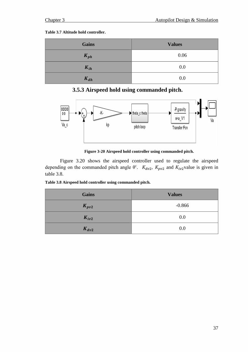
3.5.3 Airspeed hold using commanded pitch.

Figure 3-20 Airspeed hold controller using commanded pitch.

Figure 3.20 shows the airspeed controller used to regulate the airspeed

depending on the commanded pitch angle θc. 𝐾𝑑𝑣2, 𝐾𝑝𝑣2 and 𝐾𝑖𝑣2value is given in

table 3.8.

Table 3.8 Airspeed hold controller using commanded pitch.

Gains Values

𝑲𝒑𝒗𝟐 -0.866

𝑲𝒊𝒗𝟐 0.0

𝑲𝒅𝒗𝟐 0.0


38

3.5.4 Airspeed hold using throttle.

Figure 3-21 Airspeed hold controller using throttle.

Regulating the airspeed using the throttle can be done using the controller in

figure 3.21. 𝐾𝑑𝑣, 𝐾𝑝𝑣 and 𝐾𝑖𝑣 are given in table 3.9.

Table 3.9 Airspeed hold controller using throttle.

Gains Values

𝑲𝒑𝒗 1

𝑲𝒊𝒗 24

𝑲𝒅𝒗 0.0

3.6 Controller testing.

Testing is considered a very important stage in design to evaluate the

performance of the designed autopilot. There are many techniques to measure the

designed controller’s responses, here two mechanisms were used to see if the autopilot

is good enough.

3.6.1 Software in loop SIL.

The SIL simulation is a way of validation of control law performance. The

Software in the Loop Simulation builds upon the nonlinear model simulation by adding

actuator and sensor dynamics as well as integrating Simulink based flight control laws.

3.6.2 Comparison.

SIL shows if the desired control inputs were met. Here the response of the

autopilot is compared to another one in terms of gains and outputs (responses). Gains

values are obtained by a research group from University of MINNESOTA [27]. Table

3.10 shows the designed gains and classic gains used for comparison.


39

Table 3.10 Designed gains and classic gains.

Dampers P PI

Gain p

P

I

Minnesota designed Minnesota designed Minnesota designed Minnesota designed

q -0.08 -0.072

-0.84 -0.97 -0.23 -0.1

h 0.021 0.06 0.0017

P -0.07 -0.072

-0.52

-1.1216

-0.2 -0.01

1.2 4.0511 0.008

Chapter 4 Results & Discussion

40

CHAPTER4 RESULTS & DISCUSSION

4.1 Introduction

This chapter will elaborate more on the findings gathered of this project. It

presents results of the controllers introduced in sections 3.4 to 3.6. also, the performance

of the two controllers is discussed in this chapter.

4.2 Lateral controller results.

Doublet signal response

Figure 4-1 Doublet response comparison of roll tracker.

Doublet signal is concerned with the change in direction of aircraft to measure

its response due to these changes.

As shown in figure 4.1 the designed controller responds to change in input

signal quicker than Minnesota controller. This response is very useful to the

requirements of aircraft design.


41

The effects of sensors noise in the response

By assigning standard deviation σ = 1.0*10-03 rad to investigate the effect of

noise in the response.

Figure 4-2 Doublet response of roll tracker in existance of noise

The noise influences are not effectiveness in the designed controller as seen

from Figure 4.2

Multi-step of roll attitudes response

Figure 4-3 Multi step response of the roll tracker.

As can be seen from figure 4.3 a different reference input such as the multi-step

is applied to assure that the performance meets the required specifications.


42

4.2.1 Direction heading controller.

Doublet signal from standalone Simulink model.

Figure 4-4 Doublet signal response of heading angle.

From figure 4.4 we can deduce that the designed controller tracks the set point

faster than the classical controller and it has less undershoot than the classical one.

The effect of sensor noises.

The noise test is executed under the noise at sigma σ = 1*10-3 rad.

Figure 4-5 Doublet signal response of heading angle in existence of noise.

According to figure 4-5 ,the two models give almost the same response as in

figure 4-4 even in the existence of noise.


43

Rectangular motion heading command

Figure 4-6 Rectangular motion heading command response.

The designed controller has higher overshoot than the classic one, but it

responds to change faster the classic controller, but both has zero steady state error at

the end.

4.2.2 Sideslip doublet response

Figure 4-7 Doublet response to β angle


44

From figure 4.7 the designed controller proposed a good tracking of set point,

but there’s an error in the transition points.

Phi response in SIL:

Figure 4-8 Doublet signal response of the Φ angle in SIL.

According to figure 4-8, the response of the designed controller in SIL has some

ripples, but the response of the classical controller is more smoothers.

We refer this to the limitation that our controller was not tested on the

It can be seen in figures 4-1 to figure 4-8 that the overall performance of the

designed controller is the best.


45

4.3 Longitudinal controller responses.

4.3.1 Pitch Attitude Tracker Simulation Tests.

θref doublet signal response in linear Simulink.

Figure 4-9 Doublet signal response for pitch tracker.

From figure 4-9 The response of the designed controller has a smoother responseand

less overshoot comparing to the classical controller.

The effect of noise (0.001 rad) in the designed control system

Figure 4-10 Doublet signal response of pitch tracker in existence of noise.

The noise influences are not effectiveness in the designed controller as shown

in figure 4.10.


46

Multi steps response

Figure 4-11 Multi steps response for pitch tracker

As seen in figure 4-11 the two controllers have an identical response to multi

step set pint.

4.3.2 Altitude Hold Controller Simulation Tests.

The first category of tests is step response input, doublet signal and climbing

scenario response .

Step response of altitude hold controller

Figure 4-12 Step response of altitude hold controller.

From Figure 4.12 the unit step response showed that the designed controller is

obviously better in rise time and maximum overshoot and settling time.


47

10 [m] Altitude doublet signal response.

Figure 4-13 Altitude doublet signal response

The output changes against noise (0.001m).

Figure 4-14 Altitude doublet signal response with existence of noise.

According to figure 4-13 & 4-14 the designed controller still has a time analysis

characteristics better than the classical one.


48

Climbing Scenario response.

Applying climbing scenario 100 [m] then straight and leveling in the two

controllers

Figure 4-15 Climbing Scenario response.

According to figure 4-15, Simulations results illustrate that Both of the

controllers perform equally well tracking of the input signal in the straight scenario and

both of reaches the climbing level(100m) after almost 20 seconds. Yet the designed

controller has less overshoot.

Chapter 5 Conclusion & Future Work

49

CHAPTER5 CONCLUSION & FUTURE WORK

In this chapter, the state of the project, in the light of its aim and objective, is

investigated and possible future work directions are discussed.

5.1 Conclusion

The main objective of the project, which is the design and implementation of

autopilot has been done successfully, the project status can be elaborated as follows:

The longitudinal and lateral autopilot were successfully implemented

using successive loop closure and PID controller.

Using different set points such as step input, doublet signal the

performance is compared to University of Minnesota research team

controller and better performance was obtained.

SIL simulation demonstrate that PID controller is able to control with

acceptable performance the aircraft adopted for the flight tests.

5.2 Limitations

However, the system still suffers some limitations such as:

Only simulation is used in the project, the response of the designed

controller not satisfactory enough, when implemented using SIL

simulation.

By designing a PID controller, it is impossible to take into account the

uncertainties, which are present in the model parameters.

5.3 Future Work

However, the project still leaves a place for development and enhancement it

includes:

Testing the PID controller on HIL (Hardware in loop) and flight

simulator.

Using different control strategies such as LQR (Linear quadratic

Regulator) and Robust Controller.

50

REFERENCES

[1] N. Kumar and S. Jain, “Identification, Modeling and Control of Unmanned

Aerial Vehicles,” Int. J. Adv. Sci. Technol., vol. 67, pp. 1–10, 2014.

[2] R. W. B. T. W. McLAIN, SMALL UNMANNED AIRCRAFT Theory and

Practice. .

[3] J. D. Barton, “Fundamentals of Small Unmanned Aircraft Flight,” Johns

Hopkins Apl Tech. Dig., vol. 31, no. 2, pp. 132–149, 2012.

[4] T. M. Adami and J. J. Zhu, “6DOF Flight Control of Fixed-Wing Aircraft by

Trajectory Linearization,” 2011 Am. Control Conf., pp. 1610–1617, 2011.

[5] T. S. Andersen, “Master of Science in Technology Aerodynamic Modeling and

Estimation of a Fixed- wing UAV Department of technology,” 2013.

[6] a Noth, S. Bouabdallah, and R. Siegwart, “Dynamic Modeling of Fixed-Wing

UAVs,” Master Course Mech. Eng., pp. 0–11, 2006.

[7] T. I. Fossen, “MATHEMATICAL MODELS FOR CONTROL OF AIRCRAFT

AND SATELLITES,” no. February 1998, 2011.

[8] R. B. Equations, “Equations of Motion for an Unmanned Aerial,” pp. 9–23.

[9] “Rewriting the equations of motion,” pp. 1–5.

[10] S. Bagheri, “Modeling, Simulation and Control System Design for Civil

Unmanned Aerial Vehicle (UAV),” pp. 1–115, 2014.

[11] I. H. Johansen, “Autopilot Design for Unmanned Aerial Vehicles,” no. June,

2012.

[12] N. Kumar and S. Jain, “Identification , Modeling and Control of Unmanned

Aerial Vehicles,” vol. 67, pp. 1–10, 2014.

[13] C. Chen and W. Chen, “Research on Longitudinal Control Algorithm,” vol. 6,

no. 5, pp. 2155–2181, 2013.

[14] S. M. Calhoun, “SIX DEGREE OF FREEDOM,” no. June, 2006.

[15] A. Sarhan and S. Qin, “Adaptive PID Control of UAV Altitude Dynamics Based

on Parameter Optimization with Fuzzy Inference,” Int. J. Model. Optim., vol. 6,

no. 4, p. 246, 2016.

[16] B. Aliyu, A. Petinrin, and A. Adewumi, “PID Control Design of Sideslip Angle

for a FixedWing Mini-UAV,” Adv. Res., vol. 6, no. 3, pp. 1–14, 2015.

[17] D. Sartori, F. Quagliotti, M. J. Rutherford, and K. P. Valavanis, “Implementation

and Testing of a Backstepping Controller Autopilot for Fixed-wing UAVs,” J.

Intell. Robot. Syst. Theory Appl., vol. 76, no. 3–4, pp. 505–525, 2014.

[18] A. E. Ahmed, A. Hafez, A. N. Ouda, H. E. H. Ahmed, and H. M. Abd-elkader,

“Modeling of a Small Unmanned Aerial Vehicle,” Int. J. Mech. Aerospace, Ind.

Mechatron. Manuf. Eng., vol. 9, no. 3, pp. 449–457, 2015.

51

[19] “Feedback Control Systems State-Space.”

[20] “Pilot ’ s Handbook of Aeronautical Knowledge.”

[21] E. N. Mobarez, “Mathematical Representation , Modeling and Linearization for

Fixed Wing UAV,” vol. 147, no. 2, pp. 24–31, 2016.

[22] A. Dorobantu, P. J. Seiler, and G. J. Balas, “Validating Uncertain Aircraft

Simulation Models Using Flight Test Data,” pp. 1–8.

[23] M. Ahsan, K. Rafique, and F. Mazhar, “Optimization Based Tuning of Autopilot

Gains for a Fixed Wing UAV,” World Acad. Sci. Eng. Technol. Int. J. Mech.

Aerospace, Ind. Mechatron. Manuf. Eng., vol. 7, no. 5, pp. 1–6, 2013.

[24] A. Kaviyarasu and K. S. Kumar, “DESIGN OF AUTOMATIC PID GAIN

SCHEDULING FOR FIXED WING UNMANNED AERIAL VEHICLE,” no.

1, pp. 451–460.

[25] T. R. Yechout, INTRODUCTION TO AIRCRAFT FLIGHT MECHANICS,

2003rd ed. .

[26] A. Elsayed, H. Eldin, and H. Ahmed, “Design of Longitudinal Motion Controller

of a Small Unmanned Aerial Vehicle,” no. September, pp. 37–47, 2015.

[27]“UNIVERSITY OF MINNESOTA.” [Online].

Available:http://www.uav.aem.umn.edu/.

A-1

APPENDICES

Appendix A: UAV Nonlinear Simulation Setup

This script will setup the nonlinear simulation (UAV_NL.mdl) and call trim and

linearization routines. ‘Ultra-Stick 25e’ via the "UAV_config( )" function call.

% % Calls: UAV_config.m % trim_UAV.m % linearize_UAV.m % % University of Minnesota % Aerospace Engineering and Mechanics % Copyright 2011 Regents of the University of Minnesota. % All rights reserved.

%clean up clear all close all bdclose all clc

%% Add Libraries folder to MATLAB path addpath ../Libraries warning('off','Simulink:SL_LoadMdlParameterizedLink')

%% Configure Airframe, 'Ultrastick': [AC,Env] = UAV_config('Ultrastick');

%% Simulation sample time SampleTime = 0.02; % sec

%% Set aircraft initial conditions % Set the initial model inputs TrimCondition.Inputs.elevator = 0.091; % rad TrimCondition.Inputs.l_aileron = 0; % rad TrimCondition.Inputs.r_aileron = 0; % rad TrimCondition.Inputs.aileron = 0; % rad, combined aileron input TrimCondition.Inputs.rudder = 0; % rad TrimCondition.Inputs.l_flap = 0; % rad TrimCondition.Inputs.r_flap = 0; % rad TrimCondition.Inputs.throttle = 0.559; % nd, 0 to 1

% Set initial state values TrimCondition.InertialIni = [0 0 -100]'; % Initial Position in

Inertial Frame [Xe Ye Ze], [m] TrimCondition.LLIni = [44.7258357 -93.07501316]'; %

Initial Latitude/Longitude of Aircraft [Lat Long], [deg] TrimCondition.VelocitiesIni = [17 0 0.369]'; % Initial Body Frame

velocities [u v w], [m/s] TrimCondition.AttitudeIni = [0 0.0217 155*pi/180]'; % Initial

Euler orientation [roll,pitch,yaw] [rad], can't use 0 heading,

causes large entry in C matrix for psi

A-2

TrimCondition.RatesIni = [0 0 0]'; % Initial Body Frame

rotation rates [p q r], [rad/s] TrimCondition.EngineSpeedIni = 827; % Initial Engine

Speed [rad/s]

%% Trim aircraft to a specific flight condition % specify as a target.

TrimCondition.target = struct('V_s',17,'gamma',0,'h',100); %

straight and level, (m/s, rad) %TrimCondition.target = struct('V_s',17,'gamma',5/180*pi); % level

climb, (m/s, rad) %TrimCondition.target =

struct('V_s',17,'gamma',0,'psidot',20/180*pi); % level turn, (m/s,

rad, rad/sec) %TrimCondition.target =

struct('V_s',17,'gamma',5/180*pi,'psidot',20/180*pi); % climbing

turn, (m/s, rad, rad/sec) %TrimCondition.target = struct('V_s',17,'gamma',0,'beta',5/180*pi);

% level steady heading sideslip, (m/s, rad, rad)

% Find the trim solution [TrimCondition,OperatingPoint] = trim_UAV(TrimCondition,AC);

%% Linearize about the operating point

[longmod,spmod,latmod,linmodel]=linearize_UAV(OperatingPoint);

B-1

Appendix B: UAV_NL Model Verification

This script compares the linear/nonlinear doublet response of the current simulation

This script Compares the linear/nonlinear doublet response of the current

simulation %model (blue/green lines) with the check case data (red/black).

%% Full Linear Model % Full 13 state linear model. Doublets on elevator, aileron, and

rudder. load('./Verification/doublet_fullmodel.mat')

% Plot results figure(1) subplot(321), hold on plot(tsim,xsim(:,1),'r', tlin,xlin(:,7)+xsim(1,1),'k'); grid on title('Linear Velocity to Doublet Sequence

[elevator,rudder,aileron]'); xlabel('Time (sec)');ylabel('u (m/sec)') legend('NonLinear', 'Linear','Checkcase: NonLinear','Checkcase:

Linear'); subplot(323),hold on plot(tsim,xsim(:,2),'r', tlin,xlin(:,8)+xsim(1,2),'k'); grid on xlabel('Time (sec)');ylabel('v (m/sec)') subplot(325),hold on plot(tsim,xsim(:,3),'r', tlin,xlin(:,9)+xsim(1,3),'k'); grid on xlabel('Time (sec)');ylabel('w (m/sec)')

subplot(322),hold on plot(tsim,180/pi*xsim(:,10),'r',

tlin,180/pi*(xlin(:,4)+xsim(1,10)),'k'); grid on title('Angular Velocity to Doublet Sequence

[elevator,rudder,aileron]'); xlabel('Time (sec)');ylabel('p (deg/sec)') subplot(324),hold on plot(tsim,180/pi*xsim(:,11),'r',

tlin,180/pi*(xlin(:,5)+xsim(1,11)),'k'); grid on xlabel('Time (sec)');ylabel('q (deg/sec)') subplot(326),hold on plot(tsim,180/pi*xsim(:,12),'r',

tlin,180/pi*(xlin(:,6)+xsim(1,12)),'k'); grid on xlabel('Time (sec)');ylabel('r (deg/sec)')

%% Longitudinal Linear Model % Reduced order longitudinal linear model. Doublets on elevator

only. load('./Verification/doublet_longmodel.mat')

% Plot results figure(2) subplot(211),hold on plot(tsim,180/pi*ysim(:,3),'r',

tlin,180/pi*(ylin(:,2)+ysim(1,3)),'k'); grid on title('Longitudinal Model Doublet Sequence [elevator]');

B-2

xlabel('Time (sec)');ylabel('\alpha (deg)') legend('NonLinear', 'Linear','Checkcase: NonLinear','Checkcase:

Linear');


tlin,180/pi*(ylin(:,3)+xsim(1,11)),'k'); grid on xlabel('Time (sec)');ylabel('q (deg/sec)')

%% Lateral-Directional Linear Model % Reduced order lateral directional linear model. Doublets on

aileron and % rudder. load('./Verification/doublet_latmodel.mat')

% Plot results figure(3) subplot(311),hold on plot(tsim,180/pi*ysim(:,2),'r',

tlin,180/pi*(ylin(:,1)+ysim(1,2)),'k'); grid on title('Lateral-Directional Model Doublet Sequence [rudder,

aileron]'); xlabel('Time (sec)');ylabel('\beta (deg)') legend('NonLinear', 'Linear','Checkcase: NonLinear','Checkcase:

Linear');


tlin,180/pi*(ylin(:,2)+xsim(1,10)),'k'); grid on xlabel('Time (sec)');ylabel('p (deg/sec)')


tlin,180/pi*(ylin(:,3)+xsim(1,12)),'k'); grid on

xlabel('Time (sec)');ylabel('r (deg/sec)')

C-1

Appendix C: Computing Gains Code

This code is used to compute the PID controller gains using the successive loop

technique.

%%compute coefficients lambda = P.Jx*P.Jz - (P.Jxz^2); lambda_3 = P.Jz/lambda; lambda_4 = P.Jxz/lambda; C_p_p = lambda_3*P.C_ell_p + lambda_4*P.C_n_p; C_p_delta_a = lambda_3*P.C_ell_delta_a + lambda_4*P.C_n_delta_a; %%TF poles and zeros a_phi1 = -0.25*P.rho*P.Va*P.S_wing*(P.b^2)*C_p_p; a_phi2 = 0.5*P.rho*P.Va*P.Va*P.S_wing*P.b*C_p_delta_a; disp(sprintf('a_phi1 is %d:',a_phi1)); disp(sprintf('a_phi2 is %d:',a_phi2)); e_phi_max = 0.1; delta_a_max = 45; % Maximum aileron deflection zeta_phi = 0.707; phi_max = 15; omega_n_phi = sqrt(-a_phi2*delta_a_max*sqrt(1-zeta_phi^2)/phi_max); P.roll_kp = (omega_n_phi^2)/a_phi2; P.roll_kd = (2*zeta_phi*omega_n_phi - a_phi1)/a_phi2; disp(sprintf('P.roll_kp is %d:',P.roll_kp)); disp(sprintf('P.roll_kd is %d:',P.roll_kd)); disp(sprintf('omega_n_phi is %d:',omega_n_phi)); %%compute P.roll_ki using sisotool & rootlocus s = tf('s'); roll_TF=a_phi2/(s*(s^2+(a_phi1+a_phi2*P.roll_kd)*s+a_phi2*P.roll_kp

)) rlocus(roll_TF) ,sisotool(roll_TF) %------------------------------------------ omega_n_xi = 0.1*omega_n_phi; % W_xi is taken as 10, design

parameter zeta_xi = 0.707; % Design parameter damping P.heading_kp =(2*zeta_xi*omega_n_xi*P.Va)/P.gravity; P.heading_ki = (omega_n_xi^2)*P.Va/P.gravity; disp(sprintf('P.heading_kp is %d:',P.heading_kp)); disp(sprintf('P.heading_ki is %d:',P.heading_ki)); %----------------------------------- omega_n_beta = 0.05*omega_n_phi; zeta_beta = 0.707; lambda4 = P.Jxz/lambda; lambda8 = P.Jx/lambda; a_beta1 = -1*P.rho*P.Va*P.S_wing*P.C_Y_beta/(2*P.mass); a_beta2 = P.rho*P.Va*P.S_wing*P.C_Y_delta_r /(2*P.mass); e_beta_max = 0.1; delta_r_max = 25; P.beta_kp = (2*zeta_beta*omega_n_beta-a_beta1)/a_beta2; P.beta_ki = (omega_n_beta^2)/a_beta2; disp(sprintf('P.beta_kp is %d:',P.beta_kp)); disp(sprintf('P.beta_ki is %d:',P.beta_ki));

E-1

Appendix D: Baseline Controller

This code is used for comparing the roll & theta tracker of both the designed

and classic controller.

%% ======================== Lateral Control ==================%%

%% YAW DAMPER k_YD=0.065;

a_YD=-2.0; K_YD=zpk(0,a_YD,k_YD); % Washout filter K_YDz = c2d(K_YD,SampleTime); [YDz_num,YDz_den]=tfdata(K_YDz,'v'); % obtain discrete T.F.

coefficients %% ROLL TRACKER if(strcmpi(AC.aircraft,'Ultra Stick 25e')) %kp_RT= -1.1216; %ki_RT= -.01; %kp_RD= -0.072; % Roll damper %%Classical parameters kp_RT=-0.52; ki_RT=-0.2; kp_RD=-0.07;

end %% ====================== Longitudinal

Control======================% %% THETA TRACKER if(strcmpi(AC.aircraft,'Ultra Stick 25e'))

%%My parameters %kp_PT= -0.97; %ki_PT=-0.1; %kp_PD=-0.072; %Pitch damper %%Classical parameters kp_PT=-0.84; ki_PT=-0.23; kp_PD=-.08;

end

F-1

Appendix E: Heading Controller

if(strcmpi(AC.aircraft,'Ultra Stick 25e')) %%designed % Velocity Tracker kp_VT = 0.091; ki_VT = 0.02; % Altitude Tracker kp_AT = 0.021; ki_AT = 0.0 % Heading Tracker kp_HT = 1.2; %%classic % Velocity Tracker %kp_VT = .15; %ki_VT = .04; % Altitude Tracker %kp_AT= .023; %ki_AT = 0.0010; % Heading Tracker %kp_HT = 1.5;

end

% Low pass filter for altitude and velocity with pole at 2 rad/sec LP_filter=[0 0.0392;1 -.9608];

F-1

Appendix F: UAV Software-in-the-Loop Simulation

setup

This script will setup the SIL simulation. Stored aircraft configuration and trim

conditions are used.

%% Clean up %clear all %close all %bdclose all %clc

%% Add Libraries and controllers folder to MATLAB path addpath ../Libraries addpath ../Controllers

%% Load airframe configuration and trim condition % To change these, use the functions "UAV_config.m" and

"trim_UAV.m" load UAV_modelconfig load UAV_trimcondition

%% Simulation sample time SampleTime = 0.02; % sec %% Noise off, Turbulence off or on AC.Sensors.NoiseOn = 0; Env.Winds.TurbulenceOn = 0;

%% Set controller variants % Each variant corresponds to a different Simulink model that will

be % referenced in the "UAV_SIL/Control Software/Control Software"

block. flightcode_var = Simulink.Variant('controller_mode == 1 ||

controller_mode == 2); baseline_control_var = Simulink.Variant('controller_mode == 1'); heading_control_var = Simulink.Variant('controller_mode == 2');

%% Set controller mode % Use this variable to quickly change what controller is used in

the % simulation. % % 1 = baseline controller (Simulink) % 2 = Heading controller (Simulink)

controller_mode = 1;

% Load controller parameters or compile flight code switch controller_mode

case 1 % Baseline controller in Simulink. baseline_gains; % Declare baseline controller gains

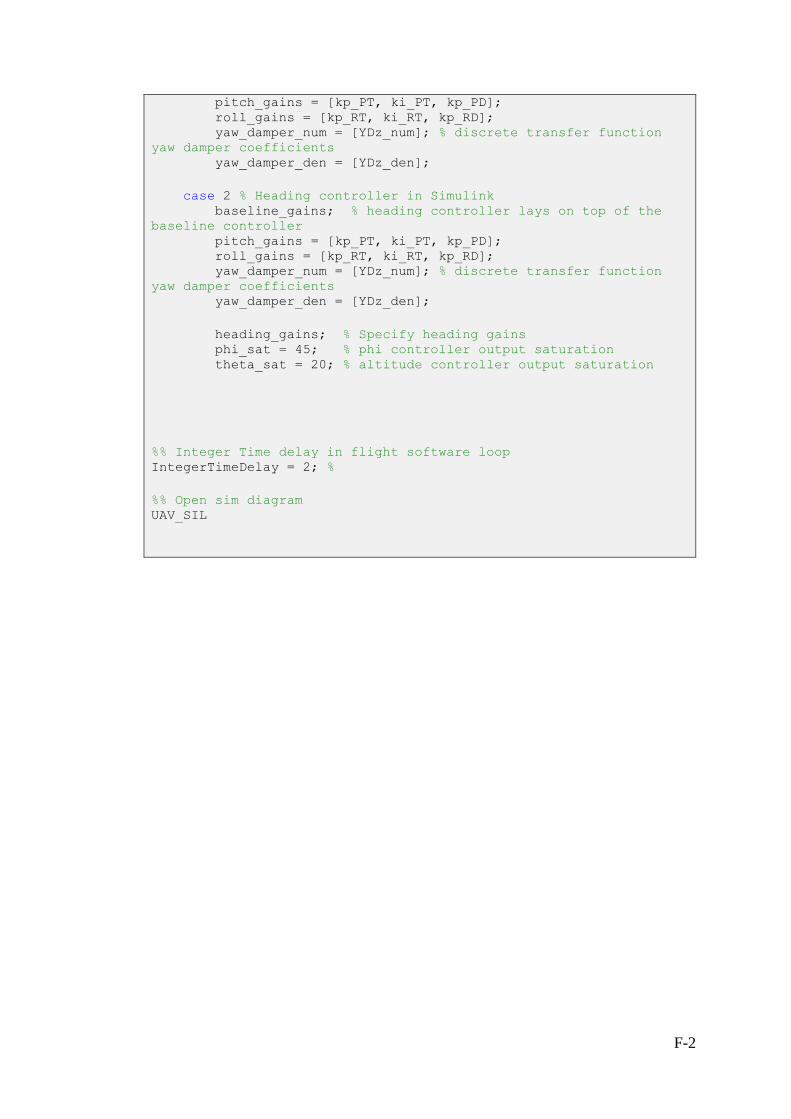
F-2

pitch_gains = [kp_PT, ki_PT, kp_PD]; roll_gains = [kp_RT, ki_RT, kp_RD]; yaw_damper_num = [YDz_num]; % discrete transfer function

yaw damper coefficients yaw_damper_den = [YDz_den];

case 2 % Heading controller in Simulink baseline_gains; % heading controller lays on top of the

baseline controller pitch_gains = [kp_PT, ki_PT, kp_PD]; roll_gains = [kp_RT, ki_RT, kp_RD]; yaw_damper_num = [YDz_num]; % discrete transfer function

yaw damper coefficients yaw_damper_den = [YDz_den];

heading_gains; % Specify heading gains phi_sat = 45; % phi controller output saturation theta_sat = 20; % altitude controller output saturation

%% Integer Time delay in flight software loop IntegerTimeDelay = 2; %

%% Open sim diagram UAV_SIL

AUTOPILOT DESIGN FOR FIXED WING UAV

Documents

Transcript of AUTOPILOT DESIGN FOR FIXED WING UAV