
Damage Tolerance Design for Wing Components
101
Damage Tolerance Design Damage Tolerance Design for Wing Components – Procedure Standardization Bernardo Vilhena Gavinho Lourenço Dissertação para obtenção do Grau de Mestre em Engenharia Aeroespacial Júri Presidente: Professor Fernando José Parracho Lau Orientador: Professor Filipe Szolnoky Ramos Pinto Cunha Co-orientador: Professor Luís Filipe Galrão dos Reis Vogais: Professor Pedro da Graça Tavares Álvares Serrão Professor Ricardo António Lamberto Duarte Cláudio Outubro de 2010
-
Upload
khangminh22 -
Category
Documents
-
view
4 -
download
0
Transcript of Damage Tolerance Design for Wing Components

Damage Tolerance Design
Damage Tolerance Design for Wing Components – Procedure
Standardization
Bernardo Vilhena Gavinho Lourenço
Dissertação para obtenção do Grau de Mestre em
Engenharia Aeroespacial
Júri
Presidente: Professor Fernando José Parracho Lau
Orientador: Professor Filipe Szolnoky Ramos Pinto Cunha
Co-orientador: Professor Luís Filipe Galrão dos Reis
Vogais: Professor Pedro da Graça Tavares Álvares Serrão
Professor Ricardo António Lamberto Duarte Cláudio
Outubro de 2010


i
Acknowledgements
The completion of this thesis was only possible with the support and guidance of many people
to whom I wish to extend my acknowledgment.
First of all, I wish to thank professors Filipe Cunha and Luís Reis for their support, guidance
and availability throughout this thesis. I also wish to thank engineers Carlos Rodrigues and Rui Pereira
for their guidance and availability during my stay in OGMA. I also wish to acknowledge Dr. Wanhill,
from the Nationaal Lucht-en Ruimtevaartlaboratorium (NLR) in the Netherlands, who kindly suggested
some important documents on Initial Damage Characterization.
A special thanks to my family and friends for their outstanding support and patience, without
them it would have been impossible.

ii
iii
Abstract
Fatigue analysis of mechanical components, in many cases, leads to underestimated lives and
thus greater costs, so a different philosophy was developed, Damage Tolerance Design. Using this
theory, the designer no longer assumes a perfect component but rather the existence of an initial
damage that is allowed to propagate. However, that damage is detected and repaired within the safety
limits placed.
The purpose of this thesis will be the definition and standardization of procedures to be
followed by an aircraft contractor, OGMA, in order to implement a Damage Tolerant Design for the
components. Once the procedure is approved by the Aeronautical Authorities it will have significant
impact on costs reduction, without compromising the safety of the repairs.
The thesis is mostly focused towards wing structures, particularly riveted joints. To do so,
stress concentration factors, residual strength determination, crack growth analysis and inspection
intervals must be correctly defined, determined and analyzed. Furthermore, the initial damage on the
structure must also be correctly assumed, in terms of shape, size, direction and quantity.
Computational methods for determining some of these parameters are mandatory.
For the concretization of the created procedure, a wing panel was analyzed using Damage
Tolerance principles.
Keywords: Damage Tolerance, Crack Propagation, Riveted Joint, Inspection Chart.

iv
v
Resumo
Uma análise de fadiga aos componentes mecânicos conduz, em muitas situações, a vidas
subestimadas e consequentemente a maiores custos, sendo por isso adoptada uma filosofia
diferente, a Tolerância ao Dano. Usando esta teoria, o projectista já não assume um componente
perfeito, mas antes que existe um dano inicial que se vai propagar, sendo este detectado e reparado
dentro dos limites de segurança impostos.
Esta tese tem como objectivo a definição e uniformização de procedimentos a serem
seguidos por uma empresa de manutenção de aeronaves, OGMA, de modo a implementar uma
filosofia de Tolerância ao Dano. Quando aprovado pelas autoridades competentes, o manual dará um
importante contributo para redução de custos, sem comprometer a segurança das manutenções.
A tese foca-se principalmente sobre estruturas em asas, em particular juntas rebitadas. Para
tal, tem de ser feita uma análise, determinação e definição detalhada de concentração de tensões,
determinação de resistência residual, análise de propagação de fendas e intervalos de inspecção.
Mais, o dano inicial existente na estrutura também tem de ser correctamente assumido, em termos de
tamanho, forma, direcção e quantidade. Os métodos computacionais assumem grande relevância na
determinação de alguns destes parâmetros.
Para concretizar o procedimento criado, foi estudado um painel de asa, usando os princípios
de Tolerância ao Dano.
Palavras-chave: Tolerância ao Dano, Propagação de Fendas, Junta Rebitada, Carta de Inspecção.

vi
vii
Contents
Acknowledgements ................................................................................................................................... i
Abstract .................................................................................................................................................... iii
Resumo .................................................................................................................................................... v
Contents ................................................................................................................................................. vii
List of Figures .......................................................................................................................................... ix
List of Tables ........................................................................................................................................... xi
Abbreviations, Acronyms and Nomenclature ........................................................................................ xiii
1. Introduction ....................................................................................................................................... 1
2. Theoretical Background of Fundamental Concepts ......................................................................... 3
2.1. Damage Tolerance Design ....................................................................................................... 3
2.2. Fracture Mechanics Design ...................................................................................................... 4
2.2.1. Energy Methods................................................................................................................ 7
2.3. Fatigue ...................................................................................................................................... 9
2.3.1. S–N Curves .................................................................................................................... 11
2.3.2. Crack Growth Rate ......................................................................................................... 11
3. Airworthiness Requirements ........................................................................................................... 15
3.1. General ................................................................................................................................... 15
3.2. Fail Safe Evaluation ................................................................................................................ 16
3.3. Safe Life Evaluation ................................................................................................................ 18
3.4. Sonic Fatigue .......................................................................................................................... 18
3.5. Damage Tolerance Evaluation ............................................................................................... 18
4. Stress Concentration Factor ........................................................................................................... 21
4.1. Rivet – State of the Art ........................................................................................................... 21
4.2. Riveted Joints ......................................................................................................................... 23
4.3. Correlation Method ................................................................................................................. 25
4.3.1. System Construction and Definition ............................................................................... 26
4.4. Finite Element Method (FEM) ................................................................................................. 27
5. Initial Damage Characterization ..................................................................................................... 29
5.1. Non Destructive Inspection Methods ...................................................................................... 29
5.2. Initial Damage Size Assumption ............................................................................................. 32
5.3. Damage Shape and Direction ................................................................................................ 35
5.4. Damage Disposition ............................................................................................................... 36
5.5. Damage Quantity .................................................................................................................... 37
5.6. Damage Location ................................................................................................................... 38
6. Load Spectrum ............................................................................................................................... 39
6.1. Wing Spectrums ..................................................................................................................... 40
6.1.1. TWIST Spectrum ............................................................................................................ 40
6.1.2. FALSTAFF Spectrum ..................................................................................................... 40
viii
6.2. Normalized Spectrum ............................................................................................................. 41
6.2.1. Complete Spectrum Normalization ................................................................................. 42
6.2.2. Spectrum Normalization per Flight Phase ...................................................................... 43
7. Residual Strength ........................................................................................................................... 45
7.1. Residual Strength on Wing Skins ........................................................................................... 46
7.1.1. Simplifications and Assumptions .................................................................................... 46
7.1.2. Requirements Application ............................................................................................... 47
7.2. Residual Strength Determination ............................................................................................ 48
8. Crack Growth Analysis ................................................................................................................... 51
8.1. Crack Retardation ................................................................................................................... 51
8.2. Stress Intensity Factor ............................................................................................................ 53
8.2.1. Stress Intensity Factor Determination in Crack Growth Analysis ................................... 54
8.3. Crack Growth Rate Determination using an Analytical Procedure ......................................... 55
8.4. Crack Growth Rate Determination using AFGROW ............................................................... 57
9. Inspection Requirements ................................................................................................................ 61
9.1. Inspection Type and Crack Detection .................................................................................... 62
9.2. Scatter Factor ......................................................................................................................... 64
9.2.1. Scatter Factor for Complete Life ..................................................................................... 65
9.2.2. Scatter Factor after First Inspection ............................................................................... 65
9.3. Initial Inspection Requirement ................................................................................................ 66
9.4. Recurrent Inspection Requirement ......................................................................................... 66
10. Example of a Damage Tolerance Analysis of a Wing Panel .......................................................... 69
11. Concluding Remarks and Future Developments ........................................................................... 75
References ............................................................................................................................................. 77
Attachments ............................................................................................................................................ 81
Attachment 1. – Utilities for Stress Concentration Factor Calculi [6]...................................................... 81
Attachment 1.1. –Stress Concentration Factor for Bearing Stress .................................................... 81
Attachment 1.2. – Stress Concentration Factor for Bypass Gross Area Stress ................................. 81
Attachment 1.3. – Bearing Distribution Factor .................................................................................... 82
Attachment 2. – Variation of Crack Detection with the Inspection‟s Conditions [45].............................. 83
Attachment 2.1. – Prior information on crack location influence on crack detection .......................... 83
Attachment 2.2. – Structural area influence on crack detection ......................................................... 83
Attachment 2.3. – Crack location influence on crack detection .......................................................... 84
Attachment 2.4. – Surface condition influence on crack detection ..................................................... 84
Attachment 2.5. – Surface condition influence on crack detection ..................................................... 84
Attachment 3. – Characteristics of the Lockheed C-130A [49] [50] ....................................................... 85
ix
List of Figures
Figure 1 – a) Crack Growth; b) Residual Strength [4] ............................................................................. 4
Figure 2 – The Three Different Stress Modes ......................................................................................... 5
Figure 3 – Crack‟s Tip Tensile Field Model Description [1] ..................................................................... 5
Figure 4 – Plastic Zone [7] ....................................................................................................................... 6
Figure 5 – Energy Release Rate for Plain Strain Cases [5] .................................................................... 7
Figure 6 – Energy Release Rate for Plain Stress Cases [5] ................................................................... 8
Figure 7 – Fatigue Process [1] ................................................................................................................ 9
Figure 8 – Fatigue Striations [1] ............................................................................................................ 10
Figure 9 – a) S-N Curve; b) Goodman Diagram [1] .............................................................................. 11
Figure 10 – a) Crack Growth Rate versus Crack Length; b) Crack Growth Rate versus Stress Intensity
Factor Range [1] .................................................................................................................................... 12
Figure 11 – Crack Growth Rate Regions [1] ......................................................................................... 12
Figure 12 – Flight Envelope................................................................................................................... 15
Figure 13 – Example of Stress Concentration near a hole [1] .............................................................. 21
Figure 14 – Different Rivet Shape [21] .................................................................................................. 22
Figure 15 – a) Normal Row; b) Staggered Row .................................................................................... 23
Figure 16 – a) Doublers; b) Splices ....................................................................................................... 24
Figure 17 – Secondary Bending [1] ....................................................................................................... 24
Figure 18 – Splice Spring System ......................................................................................................... 26
Figure 19 – Doubler Spring System ...................................................................................................... 26
Figure 20 – Finite Element Model for Splices [23] ................................................................................ 28
Figure 21 – Crack lengths and quantity [4] ............................................................................................ 29
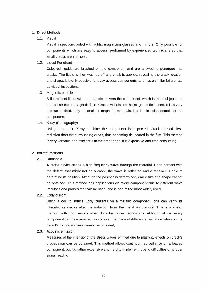
Figure 22 – Geometries for Cracks (to be used along with Table 2) [25] ............................................. 32
Figure 23 – Alternative Initial Damage Location for Countersunk Rivet Holes [28] .............................. 35
Figure 24 – Position of the crack around the fastener hole, for axial loading ....................................... 35
Figure 25 – Position of the crack around the fastener hole, for biaxial loading .................................... 36
Figure 26 – Multiple Site Damage Impact on Fatigue Life [28] ............................................................. 37
Figure 27 – Typical Manufacturing Hole Quality Damage [4] ................................................................ 38
Figure 28 – a) Normal Flight Mission; b) Typical Military Flight Mission ............................................... 39
Figure 29 – TWIST Spectrum: a) simplified; b) detailed ....................................................................... 40
Figure 30 – FALSTAFF Spectrum: a) simplified; b) detailed ................................................................. 41
Figure 31 – Normalized Spectrum per Flight Phase [1] ........................................................................ 42
Figure 32 – TWIST Spectrum after Normalization ................................................................................ 43
Figure 33 – Residual Strength Definition [4] .......................................................................................... 45
Figure 34 – Box Beam Section, Idealized using Ten Booms ................................................................ 46
Figure 35 – Wing Model for Residual Strength Determination .............................................................. 47
Figure 36 – Determination of in-section Loads...................................................................................... 49
Figure 37 – a) Cycles vs. Crack Growth; b) Stress Intensity Factor vs. Growth Rate [1] ..................... 51
x
Figure 38 – Crack Retardation Process [40] ......................................................................................... 52
Figure 39 – Crack Retardation Effects on Crack Growth [1] ................................................................. 52
Figure 40 – Superposition Method Example [1] .................................................................................... 53
Figure 41 – Fatigue Life Variation with the Loading Sequence [1]........................................................ 54
Figure 42 – Geometries Considered for Shape Factor Determination .................................................. 56
Figure 43 – Inspection‟s Detection Interval [43] .................................................................................... 61
Figure 44 – Inspections‟ Influence on Failure [44] ................................................................................ 61
Figure 45 – Crack Detection Capabilities for Different Inspection Methods [47] ................................... 63
Figure 46 – Crack Detection Interval [49] .............................................................................................. 63
Figure 47 – Scatter Factor – j2 [50]........................................................................................................ 65
Figure 48 – Recurrent Inspection Interval Definition [3] ........................................................................ 67
Figure 49 – Structure of the Lockheed C-130A Wing ........................................................................... 69
Figure 50 – Scheme for the Analyzed Wing (without Externally Mounted Probes) .............................. 69
Figure 51 – Crack Growth Prediction using AFGROW ......................................................................... 71
Figure 52 – Initial Damage Location Influence on the Panel Life .......................................................... 72
Figure 53 – Reparation to Conduct ....................................................................................................... 73
Figure 54 – Inspection Chart for Wing Root Damage ........................................................................... 73
xi
List of Tables
Table 1 – Minimum Distance between Rivets – [6] (in inches) ............................................................. 23
Table 2 – Minimum Detectable Crack Sizes – [23] (in inches) .............................................................. 31
Table 3 – Initial Crack Size Assumption – [4][22] (in inches) ................................................................ 33
Table 4 – Initial Crack Size Assumption – [25] (in inches) .................................................................... 34
Table 5 – Crack Disposition around the Hole ........................................................................................ 36
Table 6 – Number of Cracked Holes to be Introduced .......................................................................... 38
Table 7 – Spectrum‟s Main Properties .................................................................................................. 42
Table 8 – Spectrum‟s Properties per Flight Phase ................................................................................ 43
Table 9 – Geometric Models Built for Insertion on AFGROW ............................................................... 58
Table 10 – Visual Inspections‟ Characteristics [4] [43] [44] ................................................................... 62
Table 11 – Life Reduction Factors [44] ................................................................................................. 64
Table 12 – Damage and Residual Strength Data ................................................................................. 70
Table 13 – Results for Crack Growth Prediction using AFGROW ........................................................ 71
Table 14 – Inspection Requirements using a Detailed Visual Inspection ............................................. 74

xii
xiii
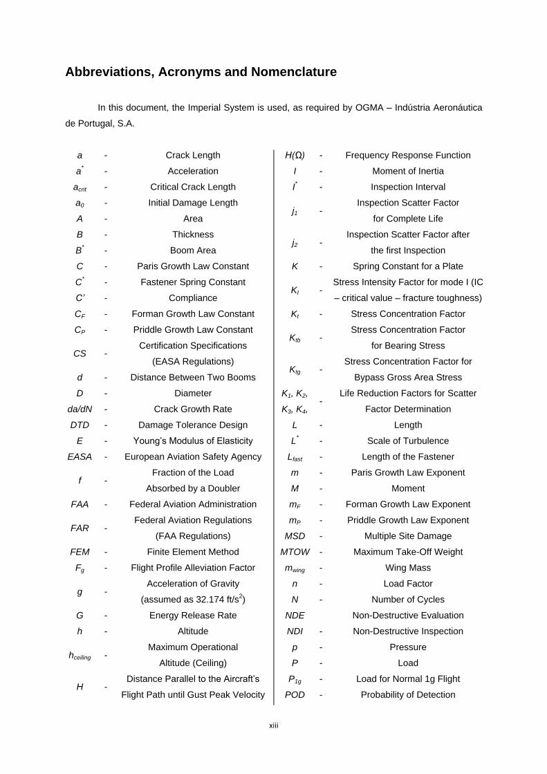
Abbreviations, Acronyms and Nomenclature
In this document, the Imperial System is used, as required by OGMA – Indústria Aeronáutica
de Portugal, S.A.
a - Crack Length
a*
- Acceleration
acrit - Critical Crack Length
a0 - Initial Damage Length
A - Area
B - Thickness
B*
- Boom Area
C - Paris Growth Law Constant
C*
- Fastener Spring Constant
C’ - Compliance
CF - Forman Growth Law Constant
CP - Priddle Growth Law Constant
CS - Certification Specifications
(EASA Regulations)
d - Distance Between Two Booms
D - Diameter
da/dN - Crack Growth Rate
DTD - Damage Tolerance Design
E - Young‟s Modulus of Elasticity
EASA - European Aviation Safety Agency
f - Fraction of the Load
Absorbed by a Doubler
FAA - Federal Aviation Administration
FAR - Federal Aviation Regulations
(FAA Regulations)
FEM - Finite Element Method
Fg - Flight Profile Alleviation Factor
g - Acceleration of Gravity
(assumed as 32.174 ft/s2)
G - Energy Release Rate
h - Altitude
hceiling - Maximum Operational
Altitude (Ceiling)
H - Distance Parallel to the Aircraft‟s
Flight Path until Gust Peak Velocity
H(Ω) - Frequency Response Function
I - Moment of Inertia
I* - Inspection Interval
j1 - Inspection Scatter Factor
for Complete Life
j2 - Inspection Scatter Factor after
the first Inspection
K - Spring Constant for a Plate
KI - Stress Intensity Factor for mode I (IC
– critical value – fracture toughness)
Kt - Stress Concentration Factor
Ktb - Stress Concentration Factor
for Bearing Stress
Ktg - Stress Concentration Factor for
Bypass Gross Area Stress
K1, K2,
K3, K4, -
Life Reduction Factors for Scatter
Factor Determination
L - Length
L* - Scale of Turbulence
Lfast - Length of the Fastener
m - Paris Growth Law Exponent
M - Moment
mF - Forman Growth Law Exponent
mP - Priddle Growth Law Exponent
MSD - Multiple Site Damage
MTOW - Maximum Take-Off Weight
mwing - Wing Mass
n - Load Factor
N - Number of Cycles
NDE Non-Destructive Evaluation
NDI - Non-Destructive Inspection
p - Pressure
P - Load
P1g - Load for Normal 1g Flight
POD - Probability of Detection
xiv
q - Shear Flow Distribution
R - Stress Ratio
R* - Crack Growth Resistance
s - Distance Penetrated in the Gust
S - In Plane Loads Applied in a Beam
Cross-section
t - Thickness
T - Tension vector
U - Elastic Energy
Udes - Design Gust Velocity
Uref - Reference Gust Velocity
USAF - United States Air Force
Uσ - Limit Turbulence Intensity
V - Velocity
VA - Maneuvering Velocity
VC - Cruise Velocity
VD - Dive Velocity
VMC - Calibrated Air Velocity
w - Plate Width
W - Weight
W *
- Crack Formation Energy
β - Shape Factor
ΔKth - Stress Intensity Factor Range in
Threshold Region
θ - Bearing Distribution Factor
θ*
Angle with the crack direction
μ - Friction Factor
ν - Poison Coefficient
ξ - Rigid Body Damping Factor
σ - Stress
σa - Alternating Stress
σmax - Maximum Stress
σm - Mean Stress
σmin - Minimum Stress
σres - Residual Strength
σys - Yield Stress
τ - Shear Stress
Ω - Reduced Frequency
1
1. Introduction
The purpose of this thesis was the development of a Damage Tolerance Design procedure, to
be used by OGMA – Indústria Aeronáutica de Portugal, S.A., one of the main aircraft maintenance
contractors in Portugal. Located in Alverca do Ribatejo, near Lisbon, the company was founded in
1918 and currently is owned by a consortium led by EADS and Embraer, with a workforce of about
1600 employees. The most important roles played by OGMA are concerned with engine and structural
maintenance and its most important maintenance contracts include several aircrafts, such as the
Lockheed C-130, P-3 Orion, F-16 Fighting Falcon, Embraer ERJ 145 family, Airbus A320 family,
among others.
Safety is the major concern for all aircraft related subjects, since the design stage through the
entire duration of the service life. Aircraft maintenance and modification must be made using certified
procedures, which guarantee safety. This procedure will allow the company to make quick estimations
on the damage tolerance capability of a structure, in accordance with EASA specifications. The thesis
will emphasize riveted joints of wings.
The certification of the procedure must be requested by OGMA to the responsible authorities,
such as EASA, which will execute a thorough evaluation in order to guarantee the safety of the
procedures there inscribed.
Since the end of the Second World War, with the increasing operational life of the aircrafts and
the introduction of jet engines, fatigue related failures started to occur. As a consequence, the study of
varied themes, like Fracture Mechanics, Fatigue, Residual Strength, Stress Concentration and Stress
Intensity Factors, was intensified. The understanding of these subjects is crucial for a good
comprehension of Damage Tolerant Design principles.
Furthermore, Damage Tolerance calculation has a great dependence on crack growth
estimations and initial crack assumptions which will display a major role during this thesis, requiring
the use of computational methods, such as FEM and AFGROW, for its determination.
Therefore, using the procedure proposed and its outputs, safe ways to ensure damage
tolerant capabilities can be applied to newly designed or repaired structures. Furthermore the costs
will be reduced, which is the primary objective for every company, as the procedure will allow the
calculus of more accurate inspection charts, assuring that damage won‟t lead to the catastrophic
failure of the structure.

2

3
2. Theoretical Background of Fundamental Concepts
2.1. Damage Tolerance Design
Fatigue related cracks are the greatest responsible for component collapse in engineering.
Thus, methods to prevent fatigue cracks from evolving to catastrophic failure where developed [1].
Safe Life was one of the first methods to be used, and it states that once a component
reaches a specified number of cycles it is replaced with a new one. This method only takes into
account fatigue life issues, and has severe economic implications, as a component will be used for a
number of cycles inferior to the one it can withstand. Nowadays, it‟s only used in critical components
of an aircraft, such as the landing gear [2].
In order to obtain a safe but economically viable component, a different approach was needed,
and thus, in the 70‟s, Damage Tolerance Design (DTD) was created.
Damage Tolerance Design is a relatively recent philosophy in structural design, usually
described as “the ability of aircraft structure to sustain anticipated loads in the presence of fatigue,
corrosion or accidental damage until such damage is detected through inspections or malfunctions
and repaired” [3].
Using DTD, the structural engineer no longer assumes a perfect structural part, like for a safe
life component, but rather assumes that the new part already has a defect that will eventually evolve
leading to the catastrophic failure of said component [3] [4].
At first sight, this theory might seem too conservative, but analysis of in service fractures and
cracking instances have indicated that a major source of cracks is the occurrence of initial
manufacturing defects, as well as service induced damage (like corrosion). As so, the consideration of
initial damage in the form of cracks or equivalent damage is absolutely necessary to ensure structural
safety.
This gives DTD a great advantage over fatigue life tests, as a much more realistic component
life prediction will be obtained, thus allowing a much more time accurate inspections‟ program.
Damage tolerant structures can be divided into two major groups:
1. Slow Crack Growth;
This category includes all types of structures, single and multiple load paths which are
designed such that initial damage will grow at a stable, slow rate and does not achieve a size large
enough to fail the structure for a specified slow crack growth period. Safety is assured by the slow rate
of growth [4].
2. Fail Safe;
Usually are structures comprised of multiple elements or load paths such that damage can be
safely contained by a failing load path or by the arrestment of a rapidly running crack at a tear strap or
other deliberate design feature [4].
Fail safe structures must meet specific residual strength requirements following the failure of
the load path or the arrestment of a running crack. Safety will be assured by the allowance of a partial
failure of the structure, the residual strength and a period of usage during which the partial failure will
4
be found.
Following this philosophy, and in order to achieve safe structures, there are several aspects
that should be taken into consideration, such as [5]:
Obtaining the residual strength as function of the crack dimension;
The allowed crack dimension;
The crack growth time;
The dimension of the pre-existent crack permitted in the structure;
The time gap between inspections, replacements or proof testing.
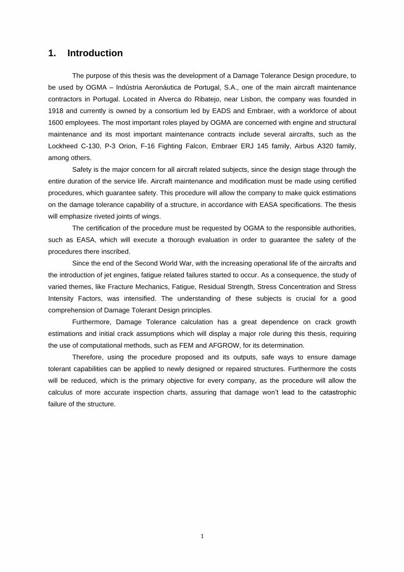
Some of the properties referred will be subject of analysis in the subsequent sections, but
through them, there are two types of graph that can be built, providing the needed information to
proceed with a damage tolerant design, in accordance with the specifications. Figure 1 presents
typical graphs that describe these properties.
Figure 1 – a) Crack Growth; b) Residual Strength [4]
In order to obtain an economically viable solution for the component, one has to ensure long
inspection periods and/or long replacement intervals. To do so the designer has several different tools
and has to take them into account for a damage tolerant design [6].
Using a different material, with better mechanical properties, with a handicap related to
the increased cost;
Improved inspection procedure;
Redesign in order to lower the stresses, as the effect of stress on crack growth is
enormous;
Use of redundant systems, in order to prevent catastrophic component failure.
2.2. Fracture Mechanics Design
Fracture mechanics has always been an important study theme in Engineering, in order to
prevent catastrophic structural failures. Its two biggest branches are Linear-Elastic and Elastic-Plastic.
This work will be mostly focused on Linear-Elastic Fracture Mechanics, which is simpler and produces
good and accurate results. One of its most important study themes is related with cracks, their sizes,
a) b)
5
shapes and growth rates. Using damage tolerance design, the existence of a crack, with
characteristics that will allow propagation, is assumed [5] [7].
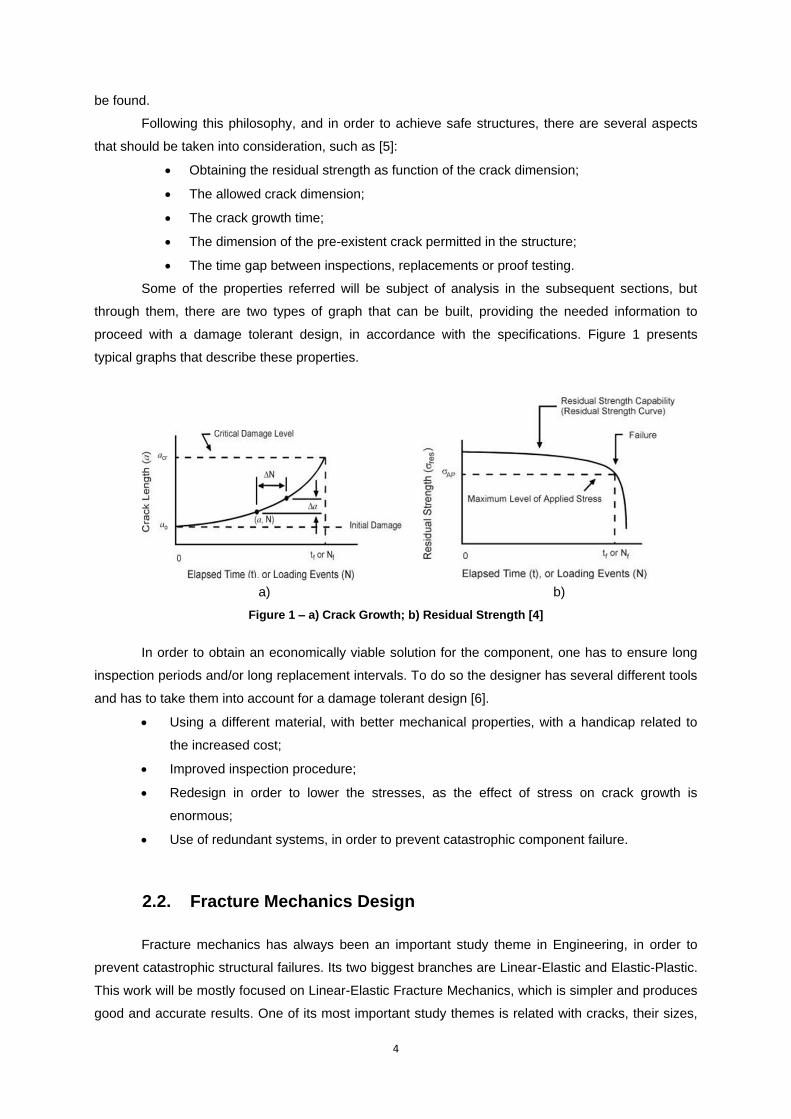
A crack in a component can be stressed in three different modes, described in Figure 2, being
mode I the most critical.
Figure 2 – The Three Different Stress Modes
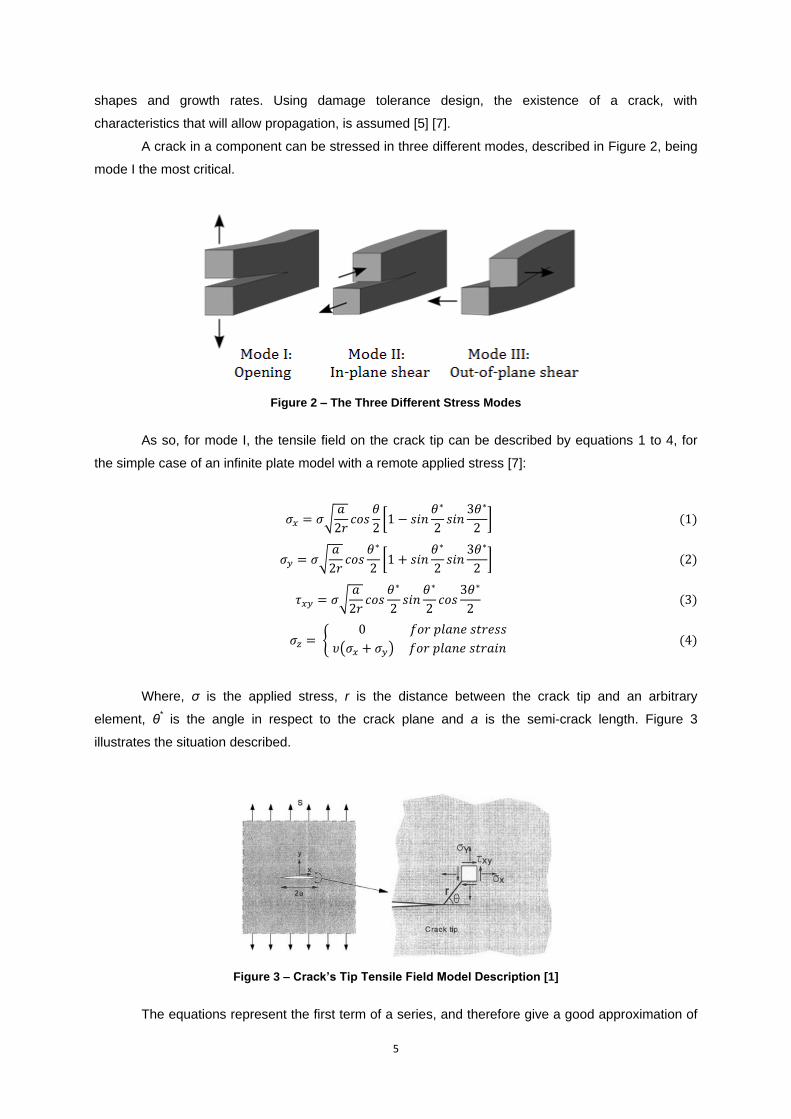
As so, for mode I, the tensile field on the crack tip can be described by equations 1 to 4, for
the simple case of an infinite plate model with a remote applied stress [7]:
Where, σ is the applied stress, r is the distance between the crack tip and an arbitrary
element, θ* is the angle in respect to the crack plane and a is the semi-crack length. Figure 3
illustrates the situation described.
Figure 3 – Crack’s Tip Tensile Field Model Description [1]
The equations represent the first term of a series, and therefore give a good approximation of
6
the crack‟s tip tensile field. As so, they can be written as:
The parameter KI is the stress intensity factor for mode I. It‟s an essentially elastic concept
that gives an indication of the stress intensity and severity near the crack‟s tip. This factor and its
variation are used to describe fatigue crack growth resistance of materials. Also the limiting value, KIC
is a property of the material, occurring when the crack reaches its critical size, known as Fracture
Toughness [1].
The critical stress intensity factor cannot be affected by different crack or component
geometries, once its limiting value defines a material property. As so the shape factor, β, is introduced,
dependent of the component, crack geometry, crack length and load applied. [7]
For an infinite plate, the shape factor will have a value near the unit, as the crack will have
neglectable size compared to the component.
For different geometries, a different β factor will be used. For simpler geometries, this factor
can be found on tables and graphs, in reference [8], but for complex geometries, its determination is
difficult and is made recurring to computational methods.
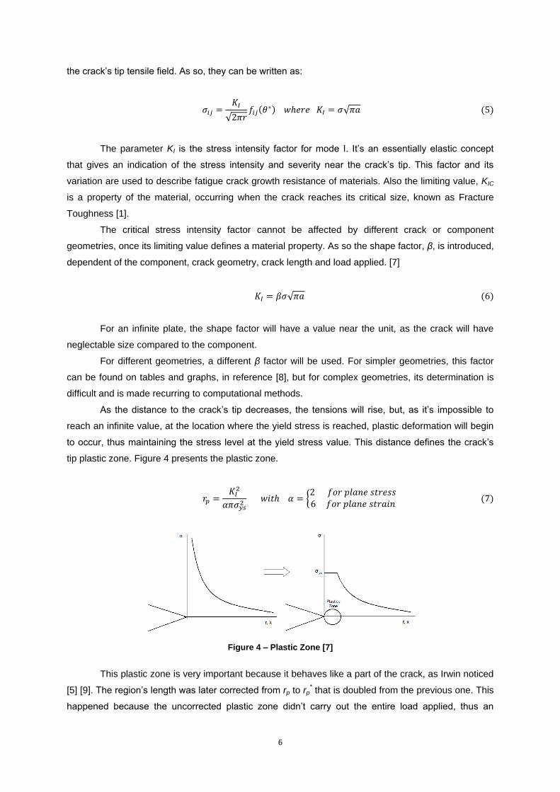
As the distance to the crack‟s tip decreases, the tensions will rise, but, as it‟s impossible to
reach an infinite value, at the location where the yield stress is reached, plastic deformation will begin
to occur, thus maintaining the stress level at the yield stress value. This distance defines the crack‟s
tip plastic zone. Figure 4 presents the plastic zone.
Figure 4 – Plastic Zone [7]
This plastic zone is very important because it behaves like a part of the crack, as Irwin noticed
[5] [9]. The region‟s length was later corrected from rp to rp* that is doubled from the previous one. This
happened because the uncorrected plastic zone didn‟t carry out the entire load applied, thus an
7
increased plastic zone would be needed [5].
The stress intensity factor determines what happens near the crack tip, particularly inside the
plastic zone, as different cracks with the same KI have similar tensile fields. This has important
consequences on crack retardation and will be discussed later on this thesis [7].
2.2.1. Energy Methods
Crack growth can occur if the system is able to provide the required energy to form an addition
to the crack length, da. This is called the Energy Release Rate, G, and can be calculated from the
elastic energy, U, and the crack resistance, R*, can be calculated from the crack formation energy, W
[5] [7].
G R*
As so, it is possible to obtain the expressions for this parameter, G, for both plain strain and
stress, considering only mode I:
Where KI is the stress intensity factor for mode I, E is the Young Modulus and υ is the Poisson
coefficient. In addition, if the component is under effects from more than one mode, the energy release
rate will be equal to the sum of the energy release of each mode.
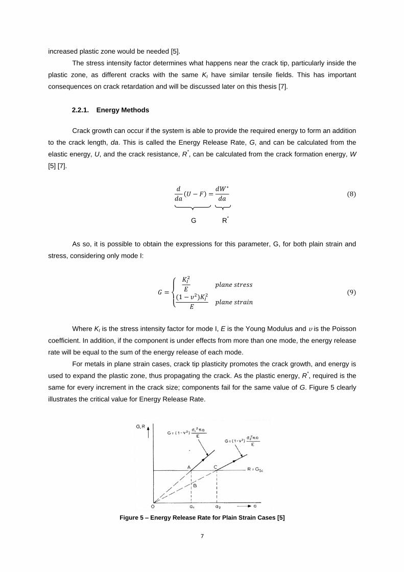
For metals in plane strain cases, crack tip plasticity promotes the crack growth, and energy is
used to expand the plastic zone, thus propagating the crack. As the plastic energy, R*, required is the
same for every increment in the crack size; components fail for the same value of G. Figure 5 clearly
illustrates the critical value for Energy Release Rate.
Figure 5 – Energy Release Rate for Plain Strain Cases [5]
8
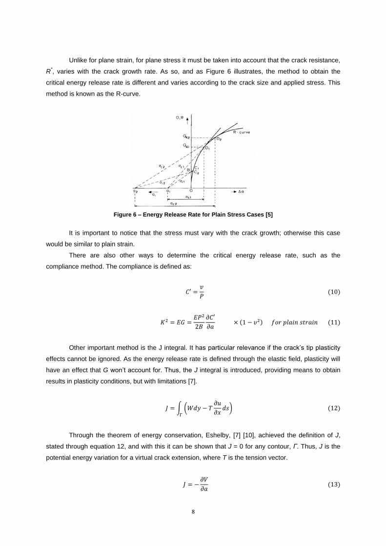
Unlike for plane strain, for plane stress it must be taken into account that the crack resistance,
R*, varies with the crack growth rate. As so, and as Figure 6 illustrates, the method to obtain the
critical energy release rate is different and varies according to the crack size and applied stress. This
method is known as the R-curve.
Figure 6 – Energy Release Rate for Plain Stress Cases [5]
It is important to notice that the stress must vary with the crack growth; otherwise this case
would be similar to plain strain.
There are also other ways to determine the critical energy release rate, such as the
compliance method. The compliance is defined as:
Other important method is the J integral. It has particular relevance if the crack‟s tip plasticity
effects cannot be ignored. As the energy release rate is defined through the elastic field, plasticity will
have an effect that G won‟t account for. Thus, the J integral is introduced, providing means to obtain
results in plasticity conditions, but with limitations [7].
Through the theorem of energy conservation, Eshelby, [7] [10], achieved the definition of J,
stated through equation 12, and with this it can be shown that J = 0 for any contour, Γ. Thus, J is the
potential energy variation for a virtual crack extension, where T is the tension vector.
9
As so, if the material behaviour is linear elastic, J = G, as expected; but in other cases a
solution is also possible. Therefore the J integral method is a more universal failure criterion.
For non linear materials the method presents limitations, as it considers component unloading
linear, fact that won‟t lead to an accurate value on the recovery energy. In spite of this limitation, this
method accounts for plasticity effects [7].
2.3. Fatigue
As mentioned, fatigue is the primary collapse reason for structural components, as so its study
and comprehension is of great importance.
This phenomenon was first acknowledged in the 19th century as a consequence of railroad
accidents, and ever since is one the most studied subjects in Engineering, based on concepts from
fracture mechanics.
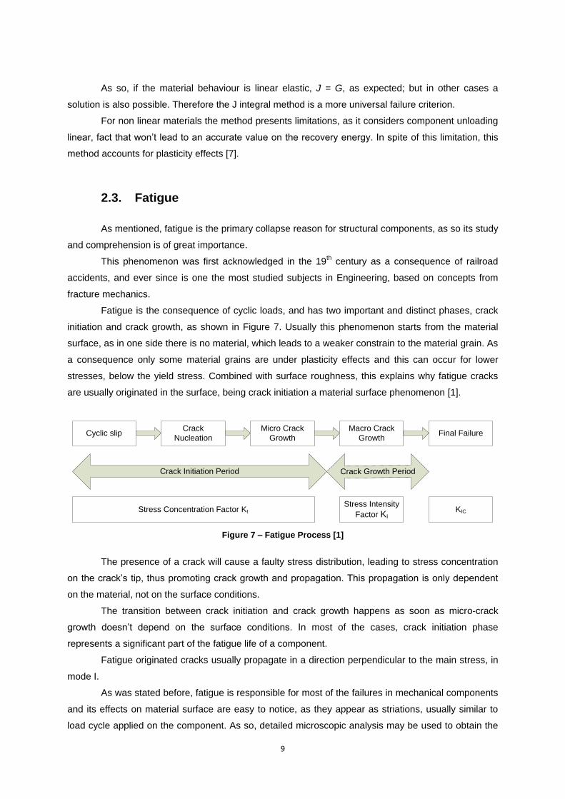
Fatigue is the consequence of cyclic loads, and has two important and distinct phases, crack
initiation and crack growth, as shown in Figure 7. Usually this phenomenon starts from the material
surface, as in one side there is no material, which leads to a weaker constrain to the material grain. As
a consequence only some material grains are under plasticity effects and this can occur for lower
stresses, below the yield stress. Combined with surface roughness, this explains why fatigue cracks
are usually originated in the surface, being crack initiation a material surface phenomenon [1].
Cyclic slipCrack
Nucleation
Micro Crack
Growth
Macro Crack
GrowthFinal Failure
Crack Initiation Period Crack Growth Period
Stress Concentration Factor Kt
Stress Intensity
Factor KIKIC
Figure 7 – Fatigue Process [1]
The presence of a crack will cause a faulty stress distribution, leading to stress concentration
on the crack‟s tip, thus promoting crack growth and propagation. This propagation is only dependent
on the material, not on the surface conditions.
The transition between crack initiation and crack growth happens as soon as micro-crack
growth doesn‟t depend on the surface conditions. In most of the cases, crack initiation phase
represents a significant part of the fatigue life of a component.
Fatigue originated cracks usually propagate in a direction perpendicular to the main stress, in
mode I.
As was stated before, fatigue is responsible for most of the failures in mechanical components
and its effects on material surface are easy to notice, as they appear as striations, usually similar to
load cycle applied on the component. As so, detailed microscopic analysis may be used to obtain the
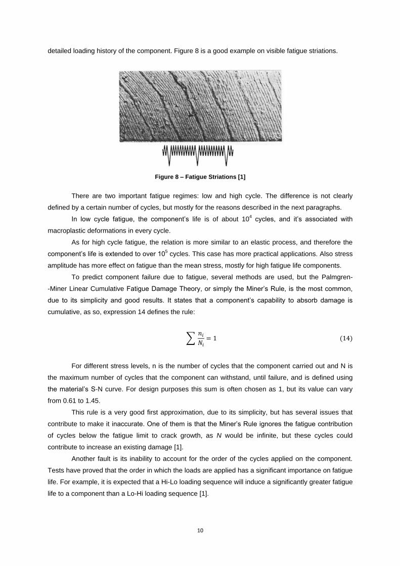
10
detailed loading history of the component. Figure 8 is a good example on visible fatigue striations.
Figure 8 – Fatigue Striations [1]
There are two important fatigue regimes: low and high cycle. The difference is not clearly
defined by a certain number of cycles, but mostly for the reasons described in the next paragraphs.
In low cycle fatigue, the component‟s life is of about 104 cycles, and it‟s associated with
macroplastic deformations in every cycle.
As for high cycle fatigue, the relation is more similar to an elastic process, and therefore the
component‟s life is extended to over 105 cycles. This case has more practical applications. Also stress
amplitude has more effect on fatigue than the mean stress, mostly for high fatigue life components.
To predict component failure due to fatigue, several methods are used, but the Palmgren-
-Miner Linear Cumulative Fatigue Damage Theory, or simply the Miner‟s Rule, is the most common,
due to its simplicity and good results. It states that a component‟s capability to absorb damage is
cumulative, as so, expression 14 defines the rule:
For different stress levels, n is the number of cycles that the component carried out and N is
the maximum number of cycles that the component can withstand, until failure, and is defined using
the material‟s S-N curve. For design purposes this sum is often chosen as 1, but its value can vary
from 0.61 to 1.45.
This rule is a very good first approximation, due to its simplicity, but has several issues that
contribute to make it inaccurate. One of them is that the Miner‟s Rule ignores the fatigue contribution
of cycles below the fatigue limit to crack growth, as N would be infinite, but these cycles could
contribute to increase an existing damage [1].
Another fault is its inability to account for the order of the cycles applied on the component.
Tests have proved that the order in which the loads are applied has a significant importance on fatigue
life. For example, it is expected that a Hi-Lo loading sequence will induce a significantly greater fatigue
life to a component than a Lo-Hi loading sequence [1].
11
2.3.1. S–N Curves
In order to predict the fatigue life of a material a diagram must be determined, called S-N
curve or Wöhler curve, in honour of one of the pioneers in fatigue tests. The line drawn in the graph
indicates critical stress level and number of cycles for a material to fail due to fatigue effects [1].
This curve is determined by fixating a stress level, and applying it in a cyclic slip until rupture
occurs or more than 10 million cycles are achieved. If this high number of cycles is achieved, the
material is said to have infinite life for the imposed stress level; this number of cycles defines the flat
zone of the curve, where fatigue life is infinite.
These curves are a material characteristic, and its determination takes a lot of time, as for
each stress level, at least two specimens are required to validate the result. Also the fatigue life
depends on the values of the mean stress and on the stress concentration factor, which establishes a
relationship between the fatigue life and the stress concentration factor that will be discussed in
Chapter 4. Still, a great compilation of S-N curves, for different material, stress ratios and stress
concentration factors, has already been created – Metallic Material Properties Development and
Standardization (MMPDS) [1] [11] [12].
The values stipulated in this curve are the fatigue limits of a material, which are used in the
Miner‟s Rule, N, representing the maximum damage allowed for the applied stress. Additionally, they
indicate the maximum expectable service period for a Safe Life component.
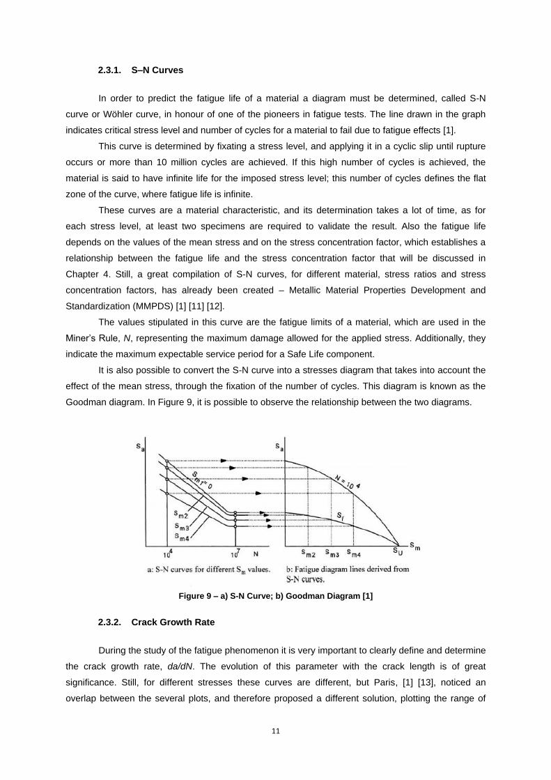
It is also possible to convert the S-N curve into a stresses diagram that takes into account the
effect of the mean stress, through the fixation of the number of cycles. This diagram is known as the
Goodman diagram. In Figure 9, it is possible to observe the relationship between the two diagrams.
Figure 9 – a) S-N Curve; b) Goodman Diagram [1]
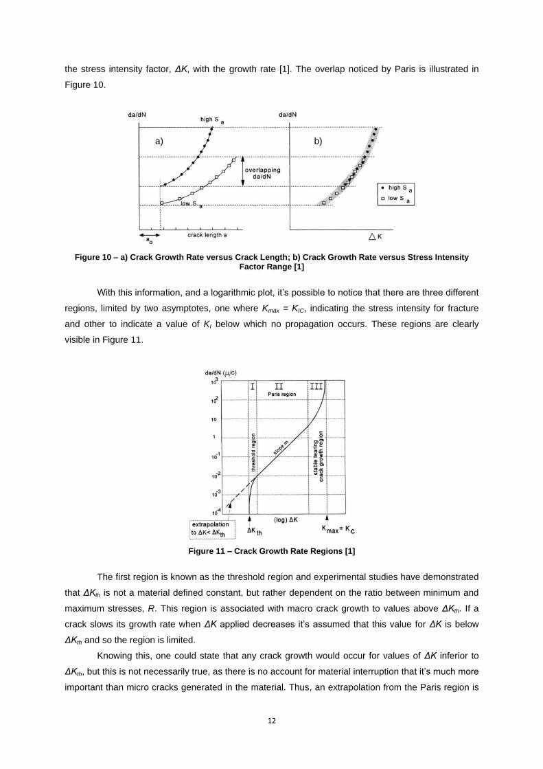
2.3.2. Crack Growth Rate
During the study of the fatigue phenomenon it is very important to clearly define and determine
the crack growth rate, da/dN. The evolution of this parameter with the crack length is of great
significance. Still, for different stresses these curves are different, but Paris, [1] [13], noticed an
overlap between the several plots, and therefore proposed a different solution, plotting the range of
12
the stress intensity factor, ΔK, with the growth rate [1]. The overlap noticed by Paris is illustrated in
Figure 10.
Figure 10 – a) Crack Growth Rate versus Crack Length; b) Crack Growth Rate versus Stress Intensity Factor Range [1]
With this information, and a logarithmic plot, it‟s possible to notice that there are three different
regions, limited by two asymptotes, one where Kmax = KIC, indicating the stress intensity for fracture
and other to indicate a value of KI below which no propagation occurs. These regions are clearly
visible in Figure 11.
Figure 11 – Crack Growth Rate Regions [1]
The first region is known as the threshold region and experimental studies have demonstrated
that ΔKth is not a material defined constant, but rather dependent on the ratio between minimum and
maximum stresses, R. This region is associated with macro crack growth to values above ΔKth. If a
crack slows its growth rate when ΔK applied decreases it‟s assumed that this value for ΔK is below
ΔKth and so the region is limited.
Knowing this, one could state that any crack growth would occur for values of ΔK inferior to
ΔKth, but this is not necessarily true, as there is no account for material interruption that it‟s much more
important than micro cracks generated in the material. Thus, an extrapolation from the Paris region is
a) b)
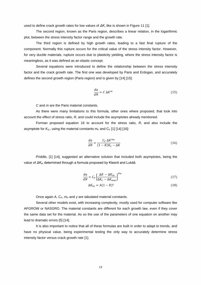
13
used to define crack growth rates for low values of ΔK, like is shown in Figure 11 [1].
The second region, known as the Paris region, describes a linear relation, in the logarithmic
plot, between the stress intensity factor range and the growth rate.
The third region is defined by high growth rates, leading to a fast final rupture of the
component. Normally this rupture occurs for the critical value of the stress intensity factor. However,
for very ductile materials, rupture occurs due to plasticity yielding, where the stress intensity factor is
meaningless, as it was defined as an elastic concept.
Several equations were introduced to define the relationship between the stress intensity
factor and the crack growth rate. The first one was developed by Paris and Erdogan, and accurately
defines the second growth region (Paris region) and is given by [14] [15]:
C and m are the Paris material constants.
As there were many limitations to this formula, other ones where proposed, that took into
account the effect of stress ratio, R, and could include the asymptotes already mentioned.
Forman proposed equation 16 to account for the stress ratio, R, and also include the
asymptote for KIC, using the material constants mF and CF [1] [14] [16]:
Priddle, [1] [14], suggested an alternative solution that included both asymptotes, being the
value of ΔKth determined through a formula proposed by Klesnil and Lukáš.
Once again A, CP, mP and γ are tabulated material constants.
Several other models exist, with increasing complexity, mostly used for computer software like
AFGROW or NASGRO. The material constants are different for each growth law, even if they cover
the same data set for the material. As so the use of the parameters of one equation on another may
lead to dramatic errors [5] [14].
It is also important to notice that all of these formulas are built in order to adapt to trends, and
have no physical value, being experimental testing the only way to accurately determine stress
intensity factor versus crack growth rate [1].

14
15
3. Airworthiness Requirements
In order to develop a damage tolerant structure, certain laws and specifications must be met.
All aircraft related laws and authority requirements can be found in FAR and CS documents; FAR for
the USA, determined by the FAA and CS for Europe, regulated by EASA. For any aircraft with a
maximum take-off weight (MTOW) higher than 12500 lbs, the documents needed to check are FAR-25
or CS-25. [17] [18]
Damage Tolerance requirements appear in sections FAR-25.571 and CS-25.571, where the
same goals are stated in both documents to achieve a damage tolerant design. Some subchapters of
this section may require the consult of other subsections in these documents.
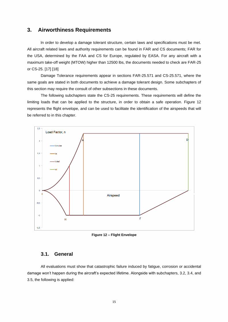
The following subchapters state the CS-25 requirements. These requirements will define the
limiting loads that can be applied to the structure, in order to obtain a safe operation. Figure 12
represents the flight envelope, and can be used to facilitate the identification of the airspeeds that will
be referred to in this chapter.
Figure 12 – Flight Envelope
3.1. General
All evaluations must show that catastrophic failure induced by fatigue, corrosion or accidental
damage won‟t happen during the aircraft‟s expected lifetime. Alongside with subchapters, 3.2, 3.4, and
3.5, the following is applied:
16
a) Evaluations must include;
i. Load spectra, temperature and humidity in flight conditions;
ii. Identification of principal structural elements, with detailed design;
iii. Detailed analysis and testing of the elements defined in 3.1.a) i..
b) Historical data from similar aircrafts, with alterations due to flight conditions;
c) Inspections must be established to prevent catastrophic failure.
3.2. Fail Safe Evaluation
The evaluation must include the determination of location and damage mode due to fatigue,
corrosion and accidental damage. This must be supported by testing, for either static and repeated
loads, or service experience. Locations exposed to prior fatigue must be included if damage is
expected to occur. For residual strength evaluation, damage extension must be consistent with the
initial detection and growth rates. Also, the evaluation must prove that the structure resists to static
ultimate loads in these conditions:
a) Normal flight envelope conditions:
Additionally
b) Gust envelope conditions:
The limit load for gust conditions has three different approaches; one for a single gust,
other for continuous turbulence and other for a gust pair.
i. For a single gust, dynamic analysis of every structural part is needed, considering
a gust with the following shape:
17
ii. In the case of continuous turbulence, the limit load is given by:
If the velocity is VD, Uσ is half of the upper value
iii. For a gust pair, one vertical and one lateral the following is applied:
Being LV and LL the loads induced by the vertical and lateral gusts, respectively,
determined using 3.2.b) i.
c) For roll maneuvering:
i. a load factor of 2/3 of the design load factor in normal flight conditions is used;
ii. Loads resulting from engine failure due to fuel flow interruption are considered
limit loads;
iii. Loads resulting from engine failure due to turbine blade loss or disconnection
between compressor and turbine are considered ultimate loads;
iv. For horizontal tails in slipstream cases are considered maximum loadings from
symmetrical conditions, plus vertical gust conditions on one side and 80% of this
load on the other side.
d) For yaw maneuvering, limited pilot force on rudder deflection of:
i. 1335 N for speeds between VMC and VA;
ii. 890 N for speeds between VC and VD;
iii. Linear variation between the upper values.
e) For pressurized fuselages, the worst case is chosen:
18
f) For landing gears:
a) A maximum vertical load factor of 1.2 for the design weight.
b) During taxi the structure is assumed to be operating under the worst ground
expected, as so, the structure is considered to be under a load factor of 2 for one
axle gears and 1.7 for multi axle gears;
3.3. Safe Life Evaluation
Compliance with subchapter 3.2 is not needed if the structure application is proven to be
unpractical. This structure must be the subject of accurate analysis and testing, proving it able to
withstand the loads expected during the predictable lifetime.
3.4. Sonic Fatigue
Analysis supported on testing or similar aircraft service history must show that:
a) Sonic fatigue cracks are not probable to appear in any structural part subjected to sonic
excitation;
b) Catastrophic failure of any structural part doesn‟t occur assuming loads as prescribed in
subchapter 3.2 applied in crack affected areas.
3.5. Damage Tolerance Evaluation
The structure must be capable of finishing a flight where structural damage occurs due to:
a) Bird strike;
The aircraft must withstand the impact of a 4 lbs bird if the relative velocity between the
aircraft and the bird doesn‟t surpass a critical value for velocity:
i. The cruise speed at sea level;
ii. 85% of the cruise speed for 8000 ft.
b) Sudden decompression of any compartment;
Every component must be designed to withstand a sudden loss of pressure, at any flight
altitude, resulting from such conditions as:
i. Engine part penetration, resulting from engine disintegration;
ii. The maximum opening caused by airplane or equipment failure that are not
extremely improbable;
iii. Any opening to the size of H0:
The maximum cross section of the pressurized compartment is given by As.

19
The fail safe features of the design should be used to determine the probability of failure
or penetration and possible opening dimensions. Improper operations on closure
devices and inadvertent door openings must be also considered. Any loads created by
the depressurization must be considered ultimate loads and be, rational and
conservatively, combined with 1g flight loads.
The main difference between FAR and CS documents, in respect to Damage Tolerance, is
that CS-25 documents make a clear definition of continued turbulence, unlike FAR-25.
Also CS-25 is more specific on gust pairs, and thus should be used to achieve a more reliable
result in such conditions, especially since this condition will most likely represent the worst case
scenario.
These reasons justify the presentation of CS-25 requirements instead of FAR-25. Even more,
this document is to be used by a European company, under EASA regulations.

20
21
4. Stress Concentration Factor
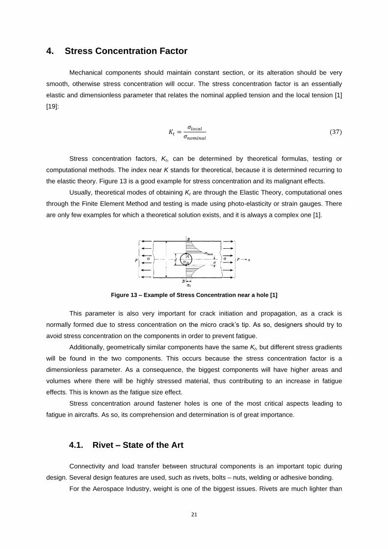
Mechanical components should maintain constant section, or its alteration should be very
smooth, otherwise stress concentration will occur. The stress concentration factor is an essentially
elastic and dimensionless parameter that relates the nominal applied tension and the local tension [1]
[19]:
Stress concentration factors, Kt, can be determined by theoretical formulas, testing or
computational methods. The index near K stands for theoretical, because it is determined recurring to
the elastic theory. Figure 13 is a good example for stress concentration and its malignant effects.
Usually, theoretical modes of obtaining Kt are through the Elastic Theory, computational ones
through the Finite Element Method and testing is made using photo-elasticity or strain gauges. There
are only few examples for which a theoretical solution exists, and it is always a complex one [1].
Figure 13 – Example of Stress Concentration near a hole [1]
This parameter is also very important for crack initiation and propagation, as a crack is
normally formed due to stress concentration on the micro crack‟s tip. As so, designers should try to
avoid stress concentration on the components in order to prevent fatigue.
Additionally, geometrically similar components have the same Kt, but different stress gradients
will be found in the two components. This occurs because the stress concentration factor is a
dimensionless parameter. As a consequence, the biggest components will have higher areas and
volumes where there will be highly stressed material, thus contributing to an increase in fatigue
effects. This is known as the fatigue size effect.
Stress concentration around fastener holes is one of the most critical aspects leading to
fatigue in aircrafts. As so, its comprehension and determination is of great importance.
4.1. Rivet – State of the Art
Connectivity and load transfer between structural components is an important topic during
design. Several design features are used, such as rivets, bolts – nuts, welding or adhesive bonding.
For the Aerospace Industry, weight is one of the biggest issues. Rivets are much lighter than
22
conventional bolts; in the other hand its installation process can be more complex and thus expensive,
unlike bolting. Also, riveted structures cannot be disassembled without destroying the fastener.
Although adhesive bonding or welding would be the lightest, the quality of the adhesive or of the weld
is a big concern and so, for safety issues, they are not used [1].
Together with adhesive bonding, rivets are one of the most ancient joining techniques known
to Mankind. They are used since Ancient Greece, as a method to join bronze parts [20] [21].
Riveting was the most important joining technique until the appearance of welding in the 19th
Century. As welding techniques produce modifications in the material atomic structure, unexpected
behaviours in fatigue processes often occur. Thus, nowadays the fields and applications for rivets
have been increasing, being the Aerospace Industry the greatest responsible.
Most rivets are installed in a predrilled hole and the tail section (opposite to the head) is then
deformed until reaching 1.5 times its original diameter to assure the rivet stays in place. In some
cases, in order to increase the joining capabilities, the rivet is inserted at a high temperature, so that
after cooling, the length reduction induced compresses the plates. The process to remove a rivet is
irreversible, as the rivet must be cut off in order to disassembly the component. This is a significant
flaw of this technique versus bolting, and introduces additional costs.
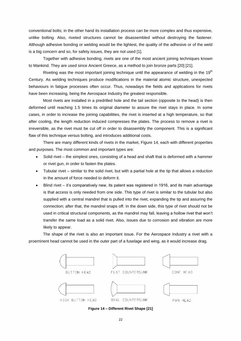
There are many different kinds of rivets in the market, Figure 14, each with different properties
and purposes. The most common and important types are:
Solid rivet – the simplest ones, consisting of a head and shaft that is deformed with a hammer
or rivet gun, in order to fasten the plates.
Tubular rivet – similar to the solid rivet, but with a partial hole at the tip that allows a reduction
in the amount of force needed to deform it.
Blind rivet – it‟s comparatively new, its patent was registered in 1916, and its main advantage
is that access is only needed from one side. This type of rivet is similar to the tubular but also
supplied with a central mandrel that is pulled into the rivet, expanding the tip and assuring the
connection; after that, the mandrel snaps off. In the down side, this type of rivet should not be
used in critical structural components, as the mandrel may fall, leaving a hollow rivet that won‟t
transfer the same load as a solid rivet. Also, issues due to corrosion and vibration are more
likely to appear.
The shape of the rivet is also an important issue. For the Aerospace Industry a rivet with a
proeminent head cannot be used in the outer part of a fuselage and wing, as it would increase drag.
Figure 14 – Different Rivet Shape [21]
23
As so, countersunk rivets are the primary choice. For this rivet shape, the hole will have to
accommodate the head, thus increasing the production costs. In spite of this fact, some aircraft use
button head rivets in the rear part of the fuselage because the airflow has so much turbulence that this
type of rivet wouldn‟t influence the aerodynamical behavouir of the structure.
Rivets can be made from several metals and different alloys. The most commonly used are
made from steel or aluminium, depending on the application and its design purpose. More recently
titanium rivets started to be introduced in aerospace applications due to its reduced weight and
superior mechanical properties. However, such fasteners still have an increased cost which leads to a
reduced market penetration.
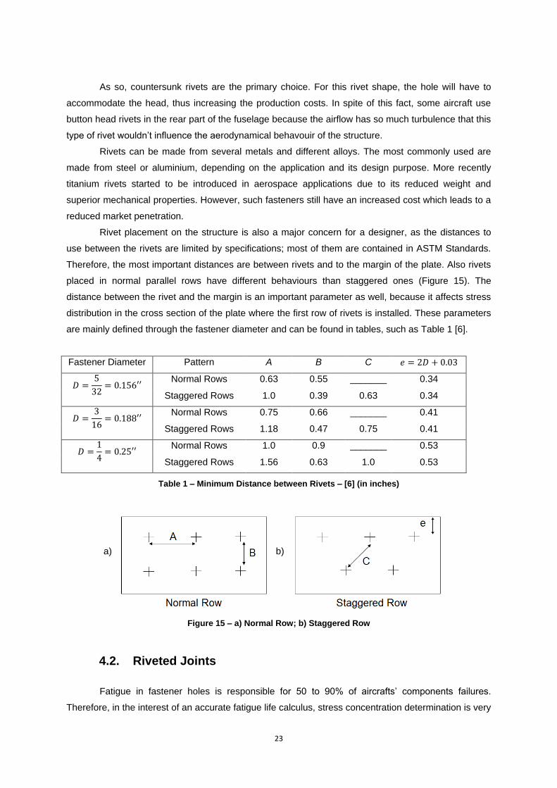
Rivet placement on the structure is also a major concern for a designer, as the distances to
use between the rivets are limited by specifications; most of them are contained in ASTM Standards.
Therefore, the most important distances are between rivets and to the margin of the plate. Also rivets
placed in normal parallel rows have different behaviours than staggered ones (Figure 15). The
distance between the rivet and the margin is an important parameter as well, because it affects stress
distribution in the cross section of the plate where the first row of rivets is installed. These parameters
are mainly defined through the fastener diameter and can be found in tables, such as Table 1 [6].
Fastener Diameter Pattern A B C
Normal Rows 0.63 0.55 _______ 0.34
Staggered Rows 1.0 0.39 0.63 0.34
Normal Rows 0.75 0.66 _______ 0.41
Staggered Rows 1.18 0.47 0.75 0.41
Normal Rows 1.0 0.9 _______ 0.53
Staggered Rows 1.56 0.63 1.0 0.53
Table 1 – Minimum Distance between Rivets – [6] (in inches)
Figure 15 – a) Normal Row; b) Staggered Row
4.2. Riveted Joints
Fatigue in fastener holes is responsible for 50 to 90% of aircrafts‟ components failures.
Therefore, in the interest of an accurate fatigue life calculus, stress concentration determination is very
a) b)
24
important in joints [22].
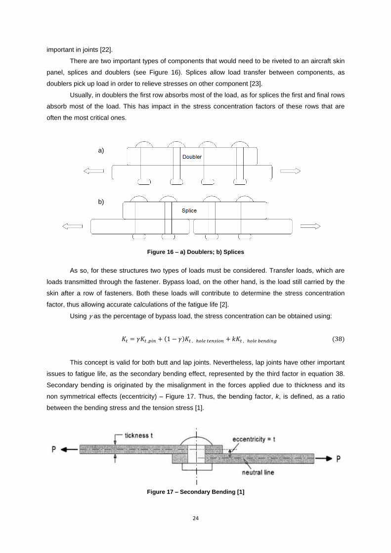
There are two important types of components that would need to be riveted to an aircraft skin
panel, splices and doublers (see Figure 16). Splices allow load transfer between components, as
doublers pick up load in order to relieve stresses on other component [23].
Usually, in doublers the first row absorbs most of the load, as for splices the first and final rows
absorb most of the load. This has impact in the stress concentration factors of these rows that are
often the most critical ones.
Figure 16 – a) Doublers; b) Splices
As so, for these structures two types of loads must be considered. Transfer loads, which are
loads transmitted through the fastener. Bypass load, on the other hand, is the load still carried by the
skin after a row of fasteners. Both these loads will contribute to determine the stress concentration
factor, thus allowing accurate calculations of the fatigue life [2].
Using γ as the percentage of bypass load, the stress concentration can be obtained using:
This concept is valid for both butt and lap joints. Nevertheless, lap joints have other important
issues to fatigue life, as the secondary bending effect, represented by the third factor in equation 38.
Secondary bending is originated by the misalignment in the forces applied due to thickness and its
non symmetrical effects (eccentricity) – Figure 17. Thus, the bending factor, k, is defined, as a ratio
between the bending stress and the tension stress [1].
Figure 17 – Secondary Bending [1]
a)
b)
25
An alternative formula to obtain Kt, used in this thesis, will be discussed in detail in subchapter
4.3.
There are features that can be used to increase fatigue life in joints. One of them is pre-
tension of the fastener, which will lead to better results on fatigue. Other method is substituting
fasteners for adhesive; it can lead to longer life, as this type of connection eliminates fretting corrosion
and stress concentration. However, durability and quality of the adhesive material must be taken into
account. In spite of these methods, the best way to improve fatigue life is avoiding stress
concentration areas during the design.
Additionally, the effect of Kt on the joint can be minored through the introduction of steps,
tapering, in the connection area that will allow a more balanced load distribution, thus leading to lower
stress concentration factors [23].
Also, crack detection is an important issue, as most of the times visual inspection is impossible
without disassembly. Pre-tension often produces a shift in the crack initiation location from the hole to
the contact point of both plates [1].
In order to determine the stress concentration factor for riveted joints there are two important
methods: an adaptation of the FEM and a correlation developed by Tom Swift in 1990. Both of these
methods must take into account fastener deflection and bearing, and also plate bearing [2] [6] [23].
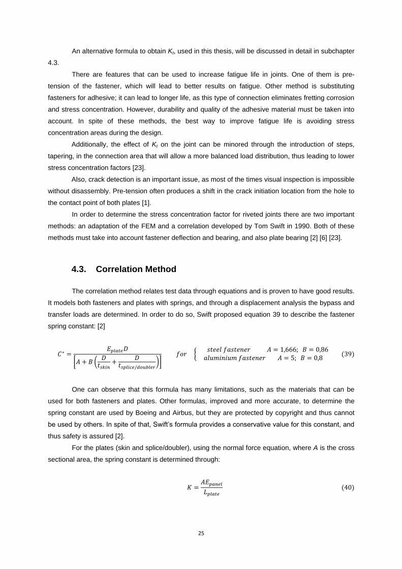
4.3. Correlation Method
The correlation method relates test data through equations and is proven to have good results.
It models both fasteners and plates with springs, and through a displacement analysis the bypass and
transfer loads are determined. In order to do so, Swift proposed equation 39 to describe the fastener
spring constant: [2]
One can observe that this formula has many limitations, such as the materials that can be
used for both fasteners and plates. Other formulas, improved and more accurate, to determine the
spring constant are used by Boeing and Airbus, but they are protected by copyright and thus cannot
be used by others. In spite of that, Swift‟s formula provides a conservative value for this constant, and
thus safety is assured [2].
For the plates (skin and splice/doubler), using the normal force equation, where A is the cross
sectional area, the spring constant is determined through:
26
4.3.1. System Construction and Definition
Knowing the fastener constant, C*, and using for the panel springs, K, it is possible to build a
matrix that relates fastener and plate displacement, and thus create a system of equations where the
only unknowns are the transfer loads in each fastener. This matrix is generated through the spring
system displacement analysis.
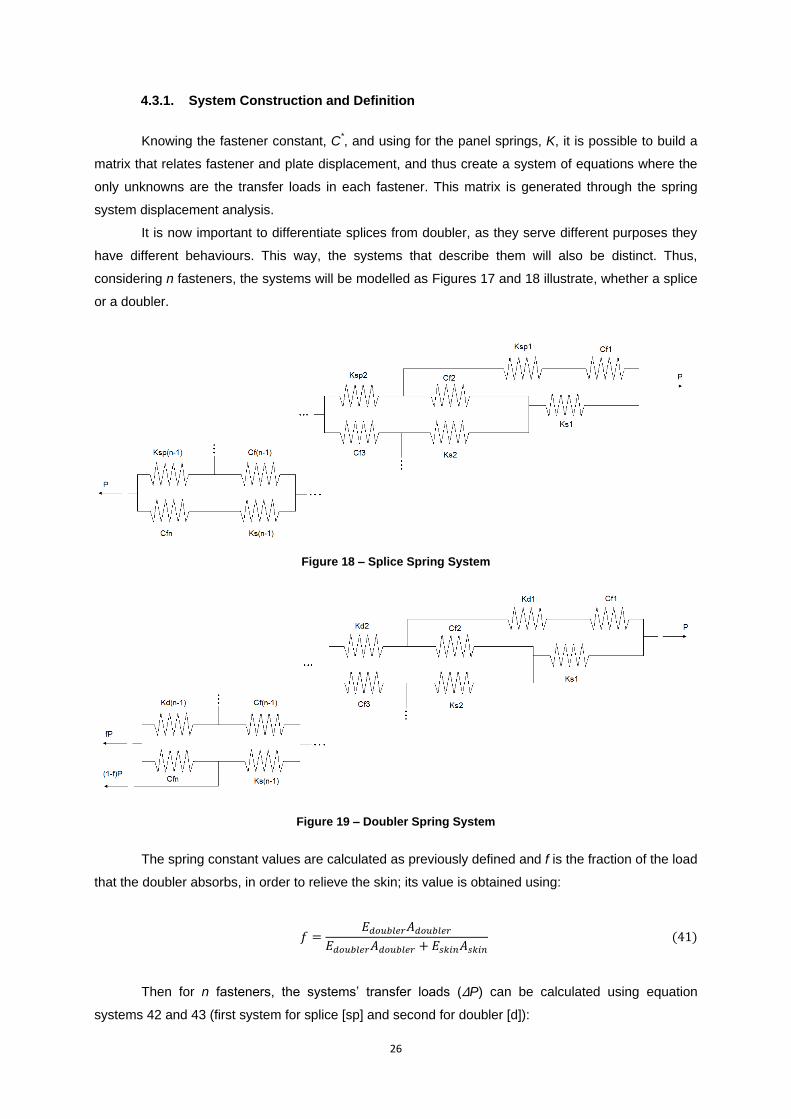
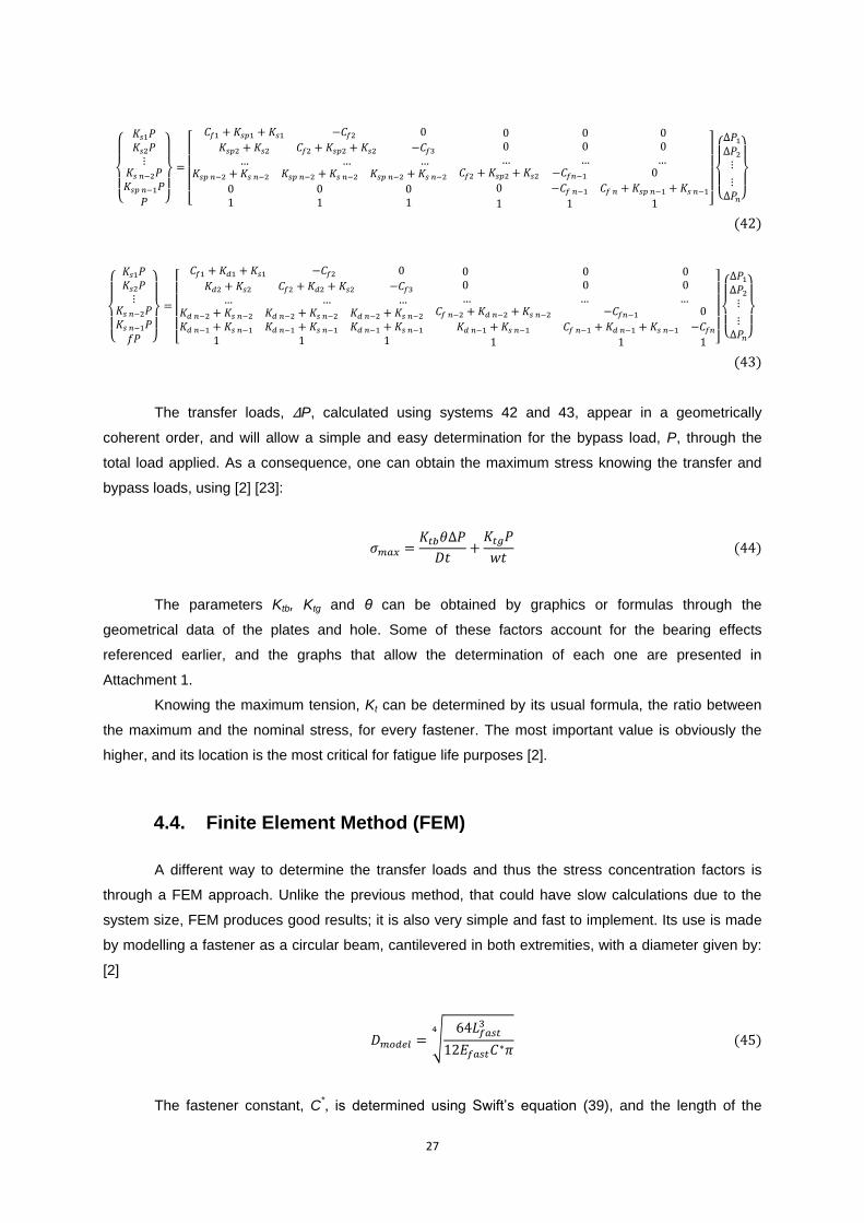
It is now important to differentiate splices from doubler, as they serve different purposes they
have different behaviours. This way, the systems that describe them will also be distinct. Thus,
considering n fasteners, the systems will be modelled as Figures 17 and 18 illustrate, whether a splice
or a doubler.
Figure 18 – Splice Spring System
Figure 19 – Doubler Spring System
The spring constant values are calculated as previously defined and f is the fraction of the load
that the doubler absorbs, in order to relieve the skin; its value is obtained using:
Then for n fasteners, the systems‟ transfer loads (ΔP) can be calculated using equation
systems 42 and 43 (first system for splice [sp] and second for doubler [d]):
27
The transfer loads, ΔP, calculated using systems 42 and 43, appear in a geometrically
coherent order, and will allow a simple and easy determination for the bypass load, P, through the
total load applied. As a consequence, one can obtain the maximum stress knowing the transfer and
bypass loads, using [2] [23]:
The parameters Ktb, Ktg and θ can be obtained by graphics or formulas through the
geometrical data of the plates and hole. Some of these factors account for the bearing effects
referenced earlier, and the graphs that allow the determination of each one are presented in
Attachment 1.
Knowing the maximum tension, Kt can be determined by its usual formula, the ratio between
the maximum and the nominal stress, for every fastener. The most important value is obviously the
higher, and its location is the most critical for fatigue life purposes [2].
4.4. Finite Element Method (FEM)
A different way to determine the transfer loads and thus the stress concentration factors is
through a FEM approach. Unlike the previous method, that could have slow calculations due to the
system size, FEM produces good results; it is also very simple and fast to implement. Its use is made
by modelling a fastener as a circular beam, cantilevered in both extremities, with a diameter given by:
[2]
The fastener constant, C*, is determined using Swift‟s equation (39), and the length of the
28
fastener is assumed unitary in order to improve calculations.
The construction of the finite element model is very simple, the fasteners are modelled as
circular cantilevered beams and linked to each other by springs, with a spring constant equal to the
one presented previously for plates (eq. 40). This way, it‟s possible to determine the bypass and
transfer loads and so, the stress concentration factor, using the same procedure that was described in
subchapter 4.3.
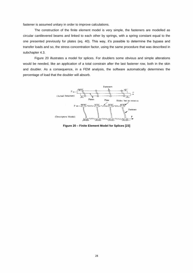
Figure 20 illustrates a model for splices. For doublers some obvious and simple alterations
would be needed, like an application of a total constrain after the last fastener row, both in the skin
and doubler. As a consequence, in a FEM analysis, the software automatically determines the
percentage of load that the doubler will absorb.
Figure 20 – Finite Element Model for Splices [23]
29
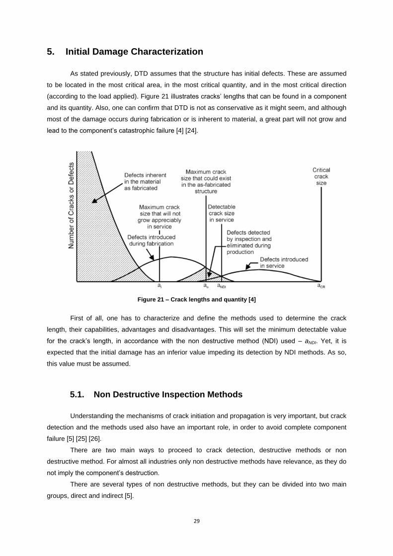
5. Initial Damage Characterization
As stated previously, DTD assumes that the structure has initial defects. These are assumed
to be located in the most critical area, in the most critical quantity, and in the most critical direction
(according to the load applied). Figure 21 illustrates cracks‟ lengths that can be found in a component
and its quantity. Also, one can confirm that DTD is not as conservative as it might seem, and although
most of the damage occurs during fabrication or is inherent to material, a great part will not grow and
lead to the component‟s catastrophic failure [4] [24].
Figure 21 – Crack lengths and quantity [4]
First of all, one has to characterize and define the methods used to determine the crack
length, their capabilities, advantages and disadvantages. This will set the minimum detectable value
for the crack‟s length, in accordance with the non destructive method (NDI) used – aNDI. Yet, it is
expected that the initial damage has an inferior value impeding its detection by NDI methods. As so,
this value must be assumed.
5.1. Non Destructive Inspection Methods
Understanding the mechanisms of crack initiation and propagation is very important, but crack
detection and the methods used also have an important role, in order to avoid complete component
failure [5] [25] [26].
There are two main ways to proceed to crack detection, destructive methods or non
destructive method. For almost all industries only non destructive methods have relevance, as they do
not imply the component‟s destruction.
There are several types of non destructive methods, but they can be divided into two main
groups, direct and indirect [5].
30
1. Direct Methods
1.1. Visual
Visual inspections aided with lights, magnifying glasses and mirrors. Only possible for
components which are easy to access, performed by experienced technicians so that
small cracks aren‟t missed;
1.2. Liquid Penetrant
Coloured liquids are brushed on the component and are allowed to penetrate into
cracks. The liquid is then washed off and chalk is applied, revealing the crack location
and shape. It is only possible for easy access components, and has a similar failure rate
as visual inspections;
1.3. Magnetic particle
A fluorescent liquid with iron particles covers the component, which is then subjected to
an intense electromagnetic field. Cracks will disturb the magnetic field lines. It is a very
precise method, only optional for magnetic materials, but implies disassemble of the
component;
1.4. X-ray (Radiography)
Using a portable X-ray machine the component is inspected. Cracks absorb less
radiation than the surrounding areas, thus becoming delineated in the film. This method
is very versatile and efficient. On the other hand, it is expensive and time consuming.
2. Indirect Methods
2.1. Ultrasonic
A probe device sends a high frequency wave through the material. Upon contact with
the defect, that might not be a crack, the wave is reflected and a receiver is able to
determine its position. Although the position is determined, crack size and shape cannot
be obtained. This method has applications on every component due to different wave
impulses and probes that can be used, and is one of the most widely used;
2.2. Eddy current
Using a coil to induce Eddy currents on a metallic component, one can verify its
integrity, as cracks alter the induction from the metal on the coil. This is a cheap
method, with good results when done by trained technicians. Although almost every
component can be examined, as coils can be made of different sizes, information on the
defect‟s nature and size cannot be obtained;
2.3. Acoustic emission
Measures of the intensity of the stress waves emitted due to plasticity effects on crack‟s
propagation can be obtained. This method allows continuum surveillance on a loaded
component, but it‟s rather expensive and hard to implement, due to difficulties on proper
signal reading.
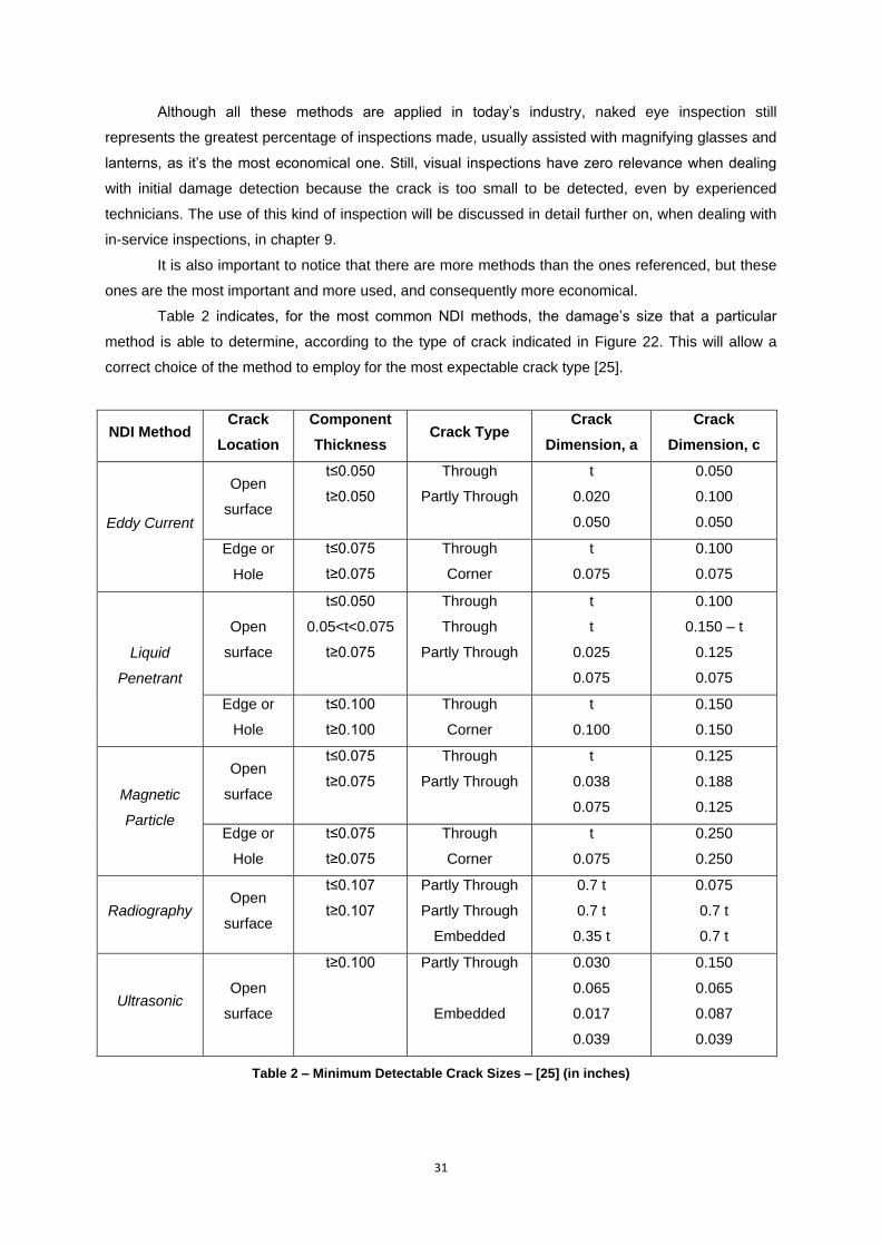
31
Although all these methods are applied in today‟s industry, naked eye inspection still
represents the greatest percentage of inspections made, usually assisted with magnifying glasses and
lanterns, as it‟s the most economical one. Still, visual inspections have zero relevance when dealing
with initial damage detection because the crack is too small to be detected, even by experienced
technicians. The use of this kind of inspection will be discussed in detail further on, when dealing with
in-service inspections, in chapter 9.
It is also important to notice that there are more methods than the ones referenced, but these
ones are the most important and more used, and consequently more economical.
Table 2 indicates, for the most common NDI methods, the damage‟s size that a particular
method is able to determine, according to the type of crack indicated in Figure 22. This will allow a
correct choice of the method to employ for the most expectable crack type [25].
NDI Method Crack
Location
Component
Thickness Crack Type
Crack
Dimension, a
Crack
Dimension, c
Eddy Current
Open
surface
t≤0.050
t≥0.050
Through
Partly Through
t
0.020
0.050
0.050
0.100
0.050
Edge or
Hole
t≤0.075
t≥0.075
Through
Corner
t
0.075
0.100
0.075
Liquid
Penetrant
Open
surface
t≤0.050
0.05<t<0.075
t≥0.075
Through
Through
Partly Through
t
t
0.025
0.075
0.100
0.150 – t
0.125
0.075
Edge or
Hole
t≤0.100
t≥0.100
Through
Corner
t
0.100
0.150
0.150
Magnetic
Particle
Open
surface
t≤0.075
t≥0.075
Through
Partly Through
t
0.038
0.075
0.125
0.188
0.125
Edge or
Hole
t≤0.075
t≥0.075
Through
Corner
t
0.075
0.250
0.250
Radiography Open
surface
t≤0.107
t≥0.107
Partly Through
Partly Through
Embedded
0.7 t
0.7 t
0.35 t
0.075
0.7 t
0.7 t
Ultrasonic Open
surface
t≥0.100 Partly Through
Embedded
0.030
0.065
0.017
0.039
0.150
0.065
0.087
0.039
Table 2 – Minimum Detectable Crack Sizes – [25] (in inches)
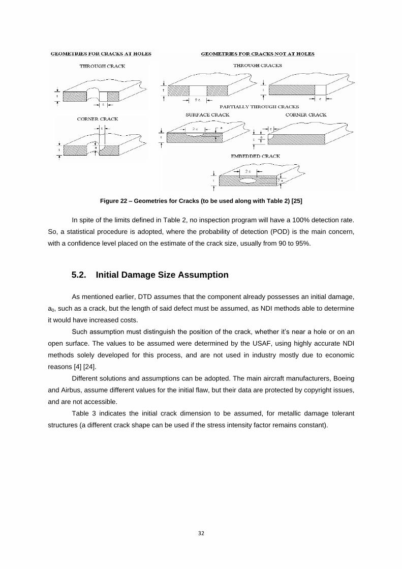
32
Figure 22 – Geometries for Cracks (to be used along with Table 2) [25]
In spite of the limits defined in Table 2, no inspection program will have a 100% detection rate.
So, a statistical procedure is adopted, where the probability of detection (POD) is the main concern,
with a confidence level placed on the estimate of the crack size, usually from 90 to 95%.
5.2. Initial Damage Size Assumption
As mentioned earlier, DTD assumes that the component already possesses an initial damage,
a0, such as a crack, but the length of said defect must be assumed, as NDI methods able to determine
it would have increased costs.
Such assumption must distinguish the position of the crack, whether it‟s near a hole or on an
open surface. The values to be assumed were determined by the USAF, using highly accurate NDI
methods solely developed for this process, and are not used in industry mostly due to economic
reasons [4] [24].
Different solutions and assumptions can be adopted. The main aircraft manufacturers, Boeing
and Airbus, assume different values for the initial flaw, but their data are protected by copyright issues,
and are not accessible.
Table 3 indicates the initial crack dimension to be assumed, for metallic damage tolerant
structures (a different crack shape can be used if the stress intensity factor remains constant).
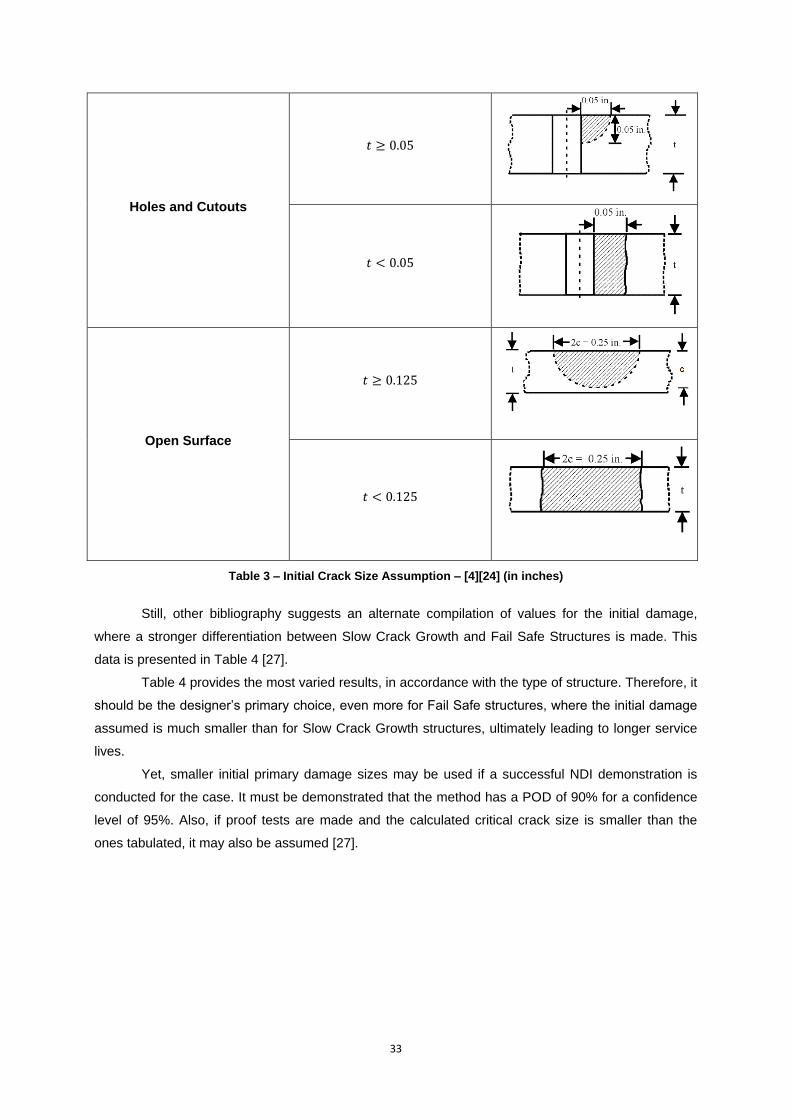
33
Holes and Cutouts
Open Surface
Table 3 – Initial Crack Size Assumption – [4][24] (in inches)
Still, other bibliography suggests an alternate compilation of values for the initial damage,
where a stronger differentiation between Slow Crack Growth and Fail Safe Structures is made. This
data is presented in Table 4 [27].
Table 4 provides the most varied results, in accordance with the type of structure. Therefore, it
should be the designer‟s primary choice, even more for Fail Safe structures, where the initial damage
assumed is much smaller than for Slow Crack Growth structures, ultimately leading to longer service
lives.
Yet, smaller initial primary damage sizes may be used if a successful NDI demonstration is
conducted for the case. It must be demonstrated that the method has a POD of 90% for a confidence
level of 95%. Also, if proof tests are made and the calculated critical crack size is smaller than the
ones tabulated, it may also be assumed [27].
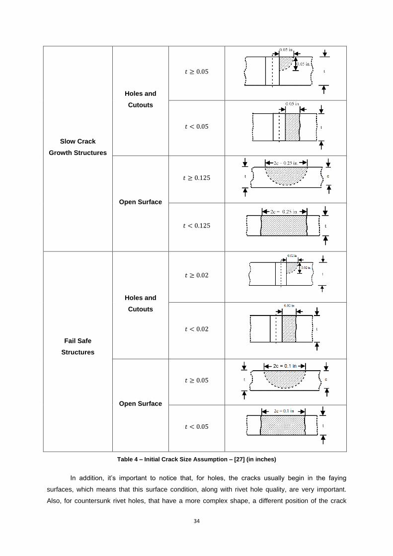
34
Slow Crack
Growth Structures
Holes and
Cutouts
Open Surface
Fail Safe
Structures
Holes and
Cutouts
Open Surface
Table 4 – Initial Crack Size Assumption – [27] (in inches)
In addition, it‟s important to notice that, for holes, the cracks usually begin in the faying
surfaces, which means that this surface condition, along with rivet hole quality, are very important.
Also, for countersunk rivet holes, that have a more complex shape, a different position of the crack
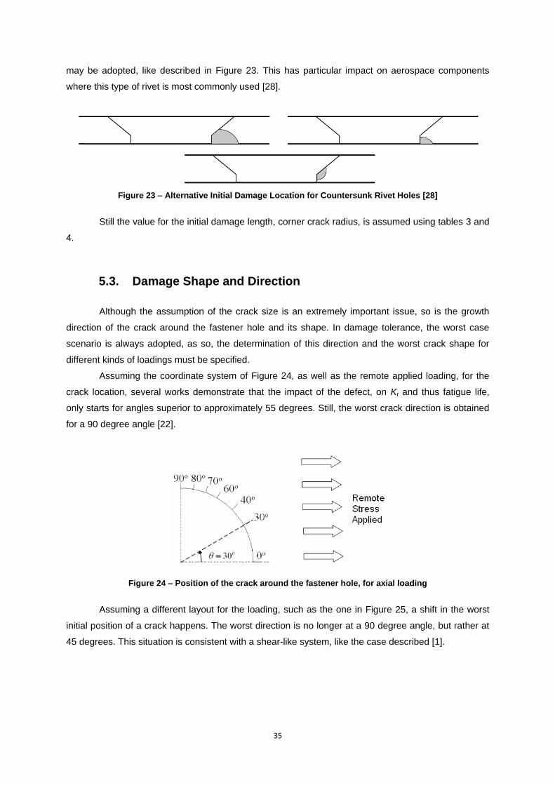
35
may be adopted, like described in Figure 23. This has particular impact on aerospace components
where this type of rivet is most commonly used [28].
Figure 23 – Alternative Initial Damage Location for Countersunk Rivet Holes [28]
Still the value for the initial damage length, corner crack radius, is assumed using tables 3 and
4.
5.3. Damage Shape and Direction
Although the assumption of the crack size is an extremely important issue, so is the growth
direction of the crack around the fastener hole and its shape. In damage tolerance, the worst case
scenario is always adopted, as so, the determination of this direction and the worst crack shape for
different kinds of loadings must be specified.
Assuming the coordinate system of Figure 24, as well as the remote applied loading, for the
crack location, several works demonstrate that the impact of the defect, on Kt and thus fatigue life,
only starts for angles superior to approximately 55 degrees. Still, the worst crack direction is obtained
for a 90 degree angle [22].
Figure 24 – Position of the crack around the fastener hole, for axial loading
Assuming a different layout for the loading, such as the one in Figure 25, a shift in the worst
initial position of a crack happens. The worst direction is no longer at a 90 degree angle, but rather at
45 degrees. This situation is consistent with a shear-like system, like the case described [1].
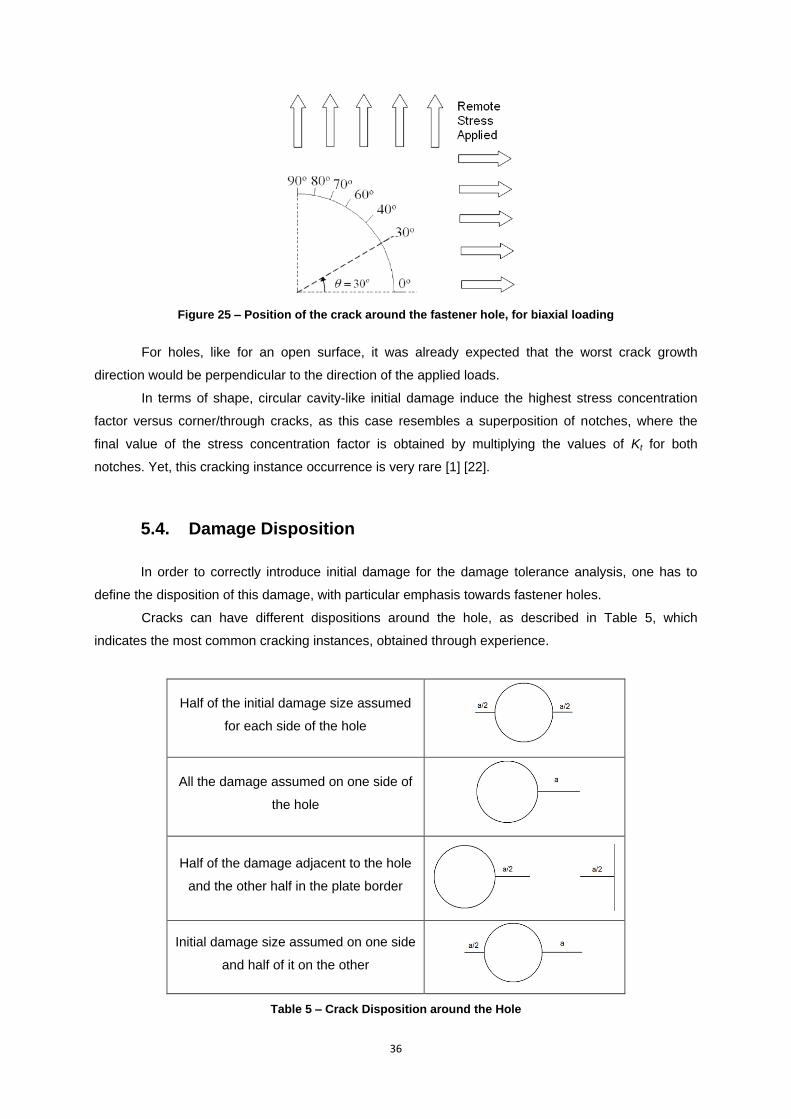
36
Figure 25 – Position of the crack around the fastener hole, for biaxial loading
For holes, like for an open surface, it was already expected that the worst crack growth
direction would be perpendicular to the direction of the applied loads.
In terms of shape, circular cavity-like initial damage induce the highest stress concentration
factor versus corner/through cracks, as this case resembles a superposition of notches, where the
final value of the stress concentration factor is obtained by multiplying the values of Kt for both
notches. Yet, this cracking instance occurrence is very rare [1] [22].
5.4. Damage Disposition
In order to correctly introduce initial damage for the damage tolerance analysis, one has to
define the disposition of this damage, with particular emphasis towards fastener holes.
Cracks can have different dispositions around the hole, as described in Table 5, which
indicates the most common cracking instances, obtained through experience.
Half of the initial damage size assumed
for each side of the hole
All the damage assumed on one side of
the hole
Half of the damage adjacent to the hole
and the other half in the plate border
Initial damage size assumed on one side
and half of it on the other
Table 5 – Crack Disposition around the Hole
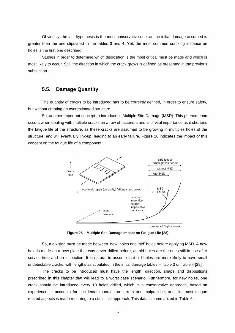
37
Obviously, the last hypothesis is the most conservative one, as the initial damage assumed is
greater than the one stipulated in the tables 3 and 4. Yet, the most common cracking instance on
holes is the first one described.
Studies in order to determine which disposition is the most critical must be made and which is
most likely to occur. Still, the direction in which the crack grows is defined as presented in the previous
subsection.
5.5. Damage Quantity
The quantity of cracks to be introduced has to be correctly defined, in order to ensure safety,
but without creating an overestimated structure.
So, another important concept to introduce is Multiple Site Damage (MSD). This phenomenon
occurs when dealing with multiple cracks on a row of fasteners and is of vital importance as it shortens
the fatigue life of the structure, as these cracks are assumed to be growing in multiples holes of the
structure, and will eventually link-up, leading to an early failure. Figure 26 indicates the impact of this
concept on the fatigue life of a component.
Figure 26 – Multiple Site Damage Impact on Fatigue Life [28]
So, a division must be made between „new‟ holes and „old‟ holes before applying MSD. A new
hole is made on a new plate that was never drilled before, as old holes are the ones still in use after
service time and an inspection. It is natural to assume that old holes are more likely to have small
undetectable cracks, with lengths as stipulated in the initial damage tables – Table 3 or Table 4 [29].
The cracks to be introduced must have the length, direction, shape and dispositions
prescribed in this chapter that will lead to a worst case scenario. Furthermore, for new holes, one
crack should be introduced every 10 holes drilled, which is a conservative approach, based on
experience. It accounts for accidental manufacture errors and malpractice, and like most fatigue
related aspects is made recurring to a statistical approach. This data is summarized in Table 6.

38
New Holes Introduction of one cracked hole
for every 10 new holes drilled
Old Holes Introduction of cracks in
every hole
Table 6 – Number of Cracked Holes to be Introduced
Furthermore, for new holes, it is assumed that every hole, where no primary initial flaw was
introduced, posseses a corner damage of 0.005 in, as shown in Figure 27, to account for the typical
manufacturing hole quality. Even more, the interference between this damage and the primary must
be properly determined. [4]
Figure 27 – Typical Manufacturing Hole Quality Damage [4]
5.6. Damage Location
The initial damage must be introduced in the worst location, in order to obtain a worst case
scenario, ensuring safety.
As mentioned in the previous chapter, for the most common systems, the first and last rows of
a splice absorb most of the load, thus being the most critical area, in terms of tension. For doublers,
the same applies for the first row, which absorbs most of the load.
Still, the area where the maximum tension is reached may not be the most critical. For
sandwich-like systems, cracks in the central skin cannot be seen by visual inspection, and therefore
may grow until obtaining critical sizes. As a consequence, cracks should be introduced in the most
critical rows of a component, whether due to the lack of inspecting capability or the existence of a
maximum stress region.
Additionally, if the cracks in the different fasteners of a row have different sizes, a “catch up”
phenomenon occurs if the ratio between the crack length, a, and the hole radius, r, is in a certain
range, determined for the problem conditions. This effect will allow many cases in which the cracks
around every fastener hole will have the same length, thus facilitating their detection by the
appropriate NDI method chosen, with smaller cracks producing a reduction in the growth rates of
larger ones [30].
Also, a cracking instance may occur due to accidental damage on a free surface, like a panel.
If so, a lead crack with the prescribed sizes and directions must be introduced in the most critical
region of said panel. Furthermore, if this lead crack has sufficient size and is formed between two
fastener holes, it will contribute to create a critical area, where failure will most likely occur [31].
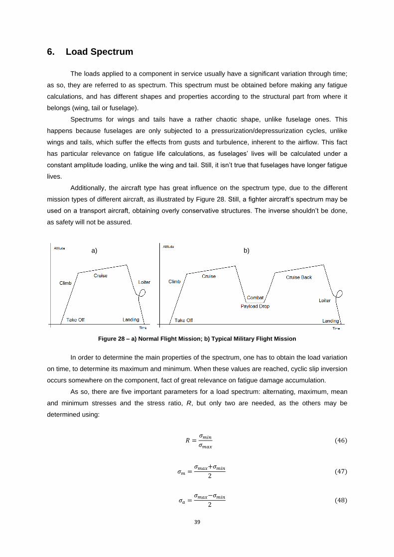
39
6. Load Spectrum
The loads applied to a component in service usually have a significant variation through time;
as so, they are referred to as spectrum. This spectrum must be obtained before making any fatigue
calculations, and has different shapes and properties according to the structural part from where it
belongs (wing, tail or fuselage).
Spectrums for wings and tails have a rather chaotic shape, unlike fuselage ones. This
happens because fuselages are only subjected to a pressurization/depressurization cycles, unlike
wings and tails, which suffer the effects from gusts and turbulence, inherent to the airflow. This fact
has particular relevance on fatigue life calculations, as fuselages‟ lives will be calculated under a
constant amplitude loading, unlike the wing and tail. Still, it isn‟t true that fuselages have longer fatigue
lives.
Additionally, the aircraft type has great influence on the spectrum type, due to the different
mission types of different aircraft, as illustrated by Figure 28. Still, a fighter aircraft‟s spectrum may be
used on a transport aircraft, obtaining overly conservative structures. The inverse shouldn‟t be done,
as safety will not be assured.
Figure 28 – a) Normal Flight Mission; b) Typical Military Flight Mission
In order to determine the main properties of the spectrum, one has to obtain the load variation
on time, to determine its maximum and minimum. When these values are reached, cyclic slip inversion
occurs somewhere on the component, fact of great relevance on fatigue damage accumulation.
As so, there are five important parameters for a load spectrum: alternating, maximum, mean
and minimum stresses and the stress ratio, R, but only two are needed, as the others may be
determined using:
a) b)
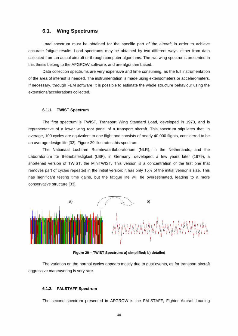
40
6.1. Wing Spectrums
Load spectrum must be obtained for the specific part of the aircraft in order to achieve
accurate fatigue results. Load spectrums may be obtained by two different ways: either from data
collected from an actual aircraft or through computer algorithms. The two wing spectrums presented in
this thesis belong to the AFGROW software, and are algorithm based.
Data collection spectrums are very expensive and time consuming, as the full instrumentation
of the area of interest is needed. The instrumentation is made using extensometers or accelerometers.
If necessary, through FEM software, it is possible to estimate the whole structure behaviour using the
extensions/accelerations collected.
6.1.1. TWIST Spectrum
The first spectrum is TWIST, Transport Wing Standard Load, developed in 1973, and is
representative of a lower wing root panel of a transport aircraft. This spectrum stipulates that, in
average, 100 cycles are equivalent to one flight and consists of nearly 40 000 flights, considered to be
an average design life [32]. Figure 29 illustrates this spectrum.
The Nationaal Lucht-en Ruimtevaartlaboratorium (NLR), in the Netherlands, and the
Laboratorium für Betriebsfestigkeit (LBF), in Germany, developed, a few years later (1979), a
shortened version of TWIST, the MiniTWIST. This version is a concentration of the first one that
removes part of cycles repeated in the initial version; it has only 15% of the initial version‟s size. This
has significant testing time gains, but the fatigue life will be overestimated, leading to a more
conservative structure [33].
Figure 29 – TWIST Spectrum: a) simplified; b) detailed
The variation on the normal cycles appears mostly due to gust events, as for transport aircraft
aggressive maneuvering is very rare.
6.1.2. FALSTAFF Spectrum
The second spectrum presented in AFGROW is the FALSTAFF, Fighter Aircraft Loading
a) b)
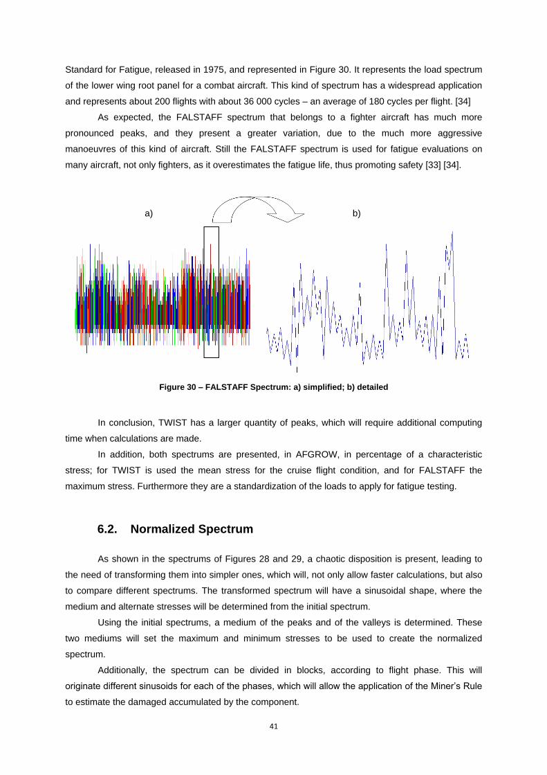
41
Standard for Fatigue, released in 1975, and represented in Figure 30. It represents the load spectrum
of the lower wing root panel for a combat aircraft. This kind of spectrum has a widespread application
and represents about 200 flights with about 36 000 cycles – an average of 180 cycles per flight. [34]
As expected, the FALSTAFF spectrum that belongs to a fighter aircraft has much more
pronounced peaks, and they present a greater variation, due to the much more aggressive
manoeuvres of this kind of aircraft. Still the FALSTAFF spectrum is used for fatigue evaluations on
many aircraft, not only fighters, as it overestimates the fatigue life, thus promoting safety [33] [34].
Figure 30 – FALSTAFF Spectrum: a) simplified; b) detailed
In conclusion, TWIST has a larger quantity of peaks, which will require additional computing
time when calculations are made.
In addition, both spectrums are presented, in AFGROW, in percentage of a characteristic
stress; for TWIST is used the mean stress for the cruise flight condition, and for FALSTAFF the
maximum stress. Furthermore they are a standardization of the loads to apply for fatigue testing.
6.2. Normalized Spectrum
As shown in the spectrums of Figures 28 and 29, a chaotic disposition is present, leading to
the need of transforming them into simpler ones, which will, not only allow faster calculations, but also
to compare different spectrums. The transformed spectrum will have a sinusoidal shape, where the
medium and alternate stresses will be determined from the initial spectrum.
Using the initial spectrums, a medium of the peaks and of the valleys is determined. These
two mediums will set the maximum and minimum stresses to be used to create the normalized
spectrum.
Additionally, the spectrum can be divided in blocks, according to flight phase. This will
originate different sinusoids for each of the phases, which will allow the application of the Miner‟s Rule
to estimate the damaged accumulated by the component.
a) b)
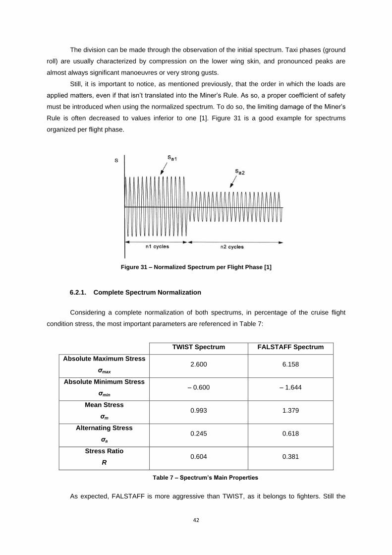
42
The division can be made through the observation of the initial spectrum. Taxi phases (ground
roll) are usually characterized by compression on the lower wing skin, and pronounced peaks are
almost always significant manoeuvres or very strong gusts.
Still, it is important to notice, as mentioned previously, that the order in which the loads are
applied matters, even if that isn‟t translated into the Miner‟s Rule. As so, a proper coefficient of safety
must be introduced when using the normalized spectrum. To do so, the limiting damage of the Miner‟s
Rule is often decreased to values inferior to one [1]. Figure 31 is a good example for spectrums
organized per flight phase.
Figure 31 – Normalized Spectrum per Flight Phase [1]
6.2.1. Complete Spectrum Normalization
Considering a complete normalization of both spectrums, in percentage of the cruise flight
condition stress, the most important parameters are referenced in Table 7:
TWIST Spectrum FALSTAFF Spectrum
Absolute Maximum Stress
σmax 2.600 6.158
Absolute Minimum Stress
σmin – 0.600 – 1.644
Mean Stress
σm 0.993 1.379
Alternating Stress
σa 0.245 0.618
Stress Ratio
R 0.604 0.381
Table 7 – Spectrum’s Main Properties
As expected, FALSTAFF is more aggressive than TWIST, as it belongs to fighters. Still the
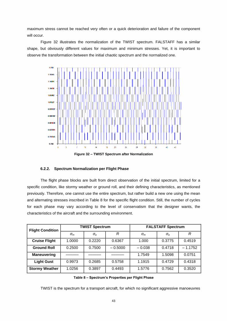
43
maximum stress cannot be reached very often or a quick deterioration and failure of the component
will occur.
Figure 32 illustrates the normalization of the TWIST spectrum. FALSTAFF has a similar
shape, but obviously different values for maximum and minimum stresses. Yet, it is important to
observe the transformation between the initial chaotic spectrum and the normalized one.
Figure 32 – TWIST Spectrum after Normalization
6.2.2. Spectrum Normalization per Flight Phase
The flight phase blocks are built from direct observation of the initial spectrum, limited for a
specific condition, like stormy weather or ground roll, and their defining characteristics, as mentioned
previously. Therefore, one cannot use the entire spectrum, but rather build a new one using the mean
and alternating stresses inscribed in Table 8 for the specific flight condition. Still, the number of cycles
for each phase may vary according to the level of conservatism that the designer wants, the
characteristics of the aircraft and the surrounding environment.
Flight Condition TWIST Spectrum FALSTAFF Spectrum
σm σa R σm σa R
Cruise Flight 1.0000 0.2220 0.6367 1.000 0.3775 0.4519
Ground Roll 0.2500 0.7500 – 0.5000 – 0.038 0.4718 – 1.1752
Maneuvering –––––– –––––– –––––– 1.7549 1.5098 0.0751
Light Gust 0.9973 0.2685 0.5758 1.1915 0.4729 0.4318
Stormy Weather 1.0256 0.3897 0.4493 1.5776 0.7562 0.3520
Table 8 – Spectrum’s Properties per Flight Phase
TWIST is the spectrum for a transport aircraft, for which no significant aggressive manoeuvres

44
exist, thus justifying the empty cells, which leads to a worst operating condition on stormy weather.
Also for FALSTAFF, the maneuvering condition presents itself as the most critical, with higher mean
and alternating stresses, according to what was expected. Furthermore, it is expected that the aircraft
has a more intensive and thorough maintenance program after long combat/maneuvering periods
occur.
Even more, for both spectrums, long periods on stormy weather may require shorter
inspection intervals, in order to ensure that safety has not been compromised.
Both normalizations demonstrate that FALSTAFF is much more aggressive than TWIST, as
expected, once it belongs to a fighter.
The difference between these two spectrums has severe consequences on fatigue life, as the
same component under FALSTAFF spectrum is expected to have less life time until failure. Yet, and
as referenced, its use for non-fighter aircraft will consist on a conservative approach, leading to a safe,
but overestimated structure. This type of reasoning is often used as it consists on the introduction of a
safety factor.
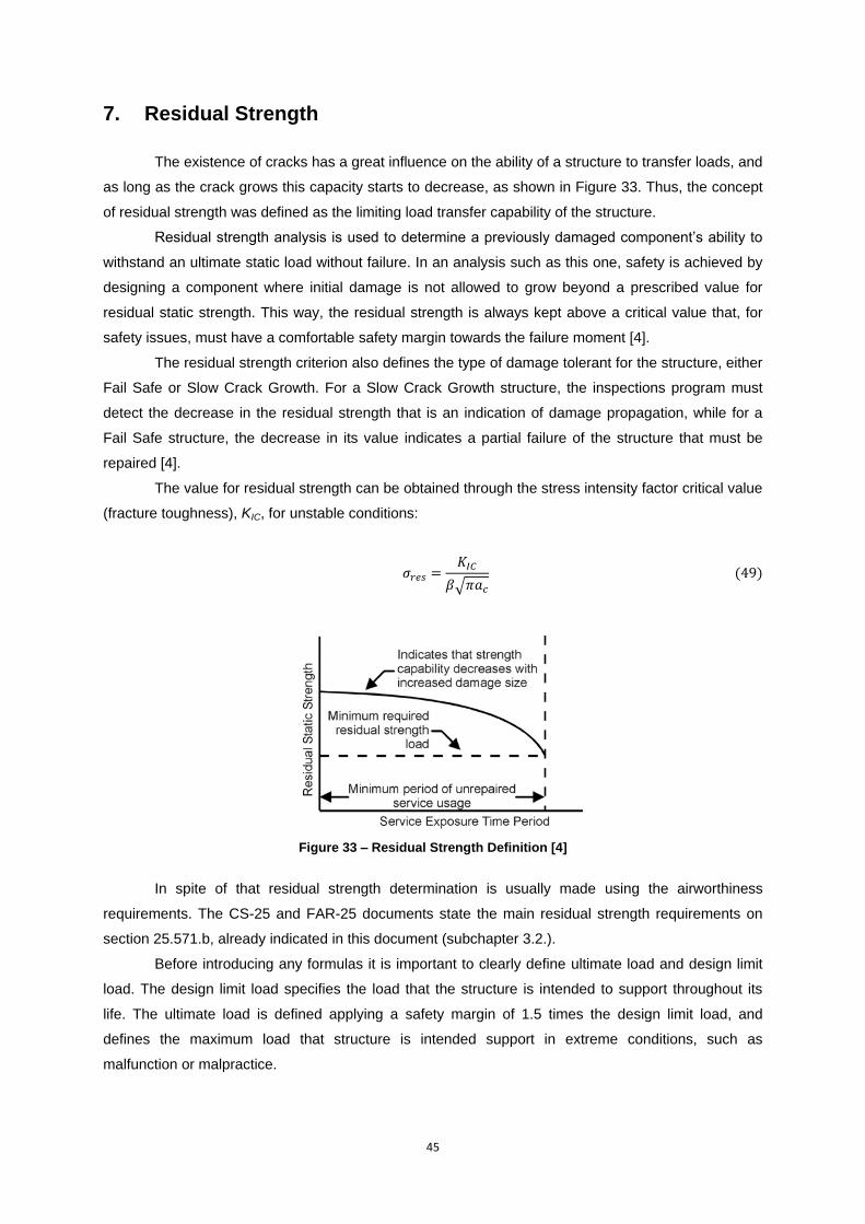
45
7. Residual Strength
The existence of cracks has a great influence on the ability of a structure to transfer loads, and
as long as the crack grows this capacity starts to decrease, as shown in Figure 33. Thus, the concept
of residual strength was defined as the limiting load transfer capability of the structure.
Residual strength analysis is used to determine a previously damaged component‟s ability to
withstand an ultimate static load without failure. In an analysis such as this one, safety is achieved by
designing a component where initial damage is not allowed to grow beyond a prescribed value for
residual static strength. This way, the residual strength is always kept above a critical value that, for
safety issues, must have a comfortable safety margin towards the failure moment [4].
The residual strength criterion also defines the type of damage tolerant for the structure, either
Fail Safe or Slow Crack Growth. For a Slow Crack Growth structure, the inspections program must
detect the decrease in the residual strength that is an indication of damage propagation, while for a
Fail Safe structure, the decrease in its value indicates a partial failure of the structure that must be
repaired [4].
The value for residual strength can be obtained through the stress intensity factor critical value
(fracture toughness), KIC, for unstable conditions:
Figure 33 – Residual Strength Definition [4]
In spite of that residual strength determination is usually made using the airworthiness
requirements. The CS-25 and FAR-25 documents state the main residual strength requirements on
section 25.571.b, already indicated in this document (subchapter 3.2.).
Before introducing any formulas it is important to clearly define ultimate load and design limit
load. The design limit load specifies the load that the structure is intended to support throughout its
life. The ultimate load is defined applying a safety margin of 1.5 times the design limit load, and
defines the maximum load that structure is intended support in extreme conditions, such as
malfunction or malpractice.
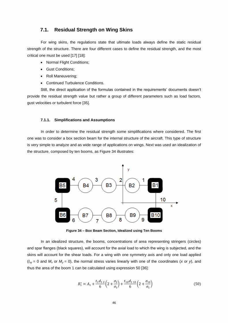
46
7.1. Residual Strength on Wing Skins
For wing skins, the regulations state that ultimate loads always define the static residual
strength of the structure. There are four different cases to define the residual strength, and the most
critical one must be used [17] [18]:
Normal Flight Conditions;
Gust Conditions;
Roll Maneuvering;
Continued Turbulence Conditions.
Still, the direct application of the formulas contained in the requirements‟ documents doesn‟t
provide the residual strength value but rather a group of different parameters such as load factors,
gust velocities or turbulent force [35].
7.1.1. Simplifications and Assumptions
In order to determine the residual strength some simplifications where considered. The first
one was to consider a box section beam for the internal structure of the aircraft. This type of structure
is very simple to analyze and as wide range of applications on wings. Next was used an idealization of
the structure, composed by ten booms, as Figure 34 illustrates:
Figure 34 – Box Beam Section, Idealized using Ten Booms
In an idealized structure, the booms, concentrations of area representing stringers (circles)
and spar flanges (black squares), will account for the axial load to which the wing is subjected, and the
skins will account for the shear loads. For a wing with one symmetry axis and only one load applied
(Ixy = 0 and Mx or My = 0), the normal stress varies linearly with one of the coordinates (x or y), and
thus the area of the boom 1 can be calculated using expression 50 [36]:
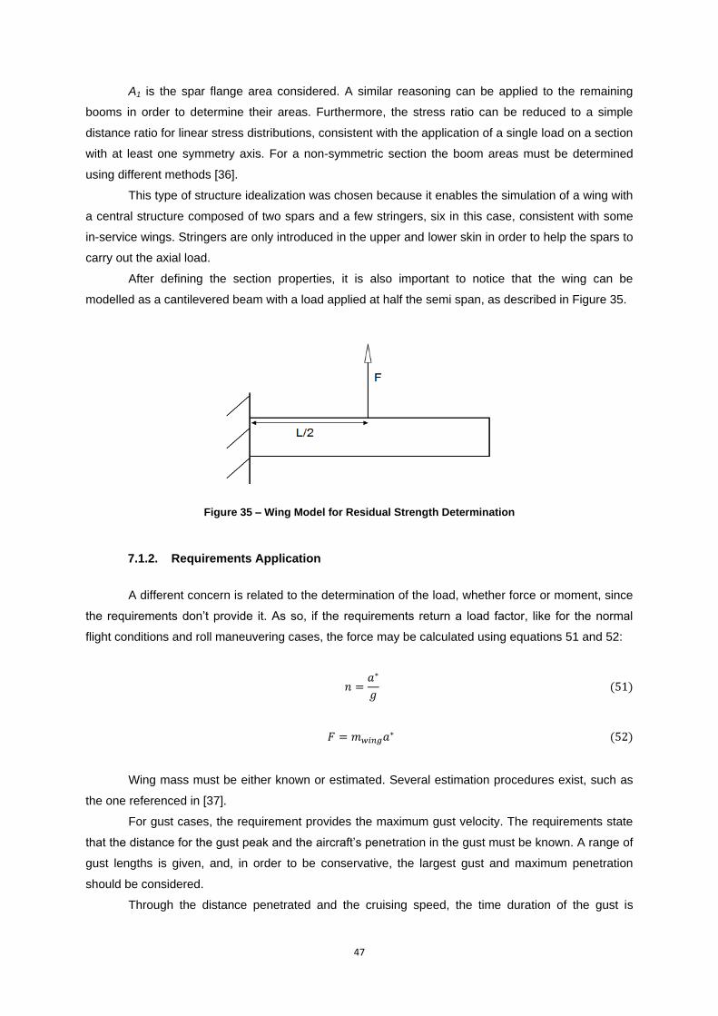
47
A1 is the spar flange area considered. A similar reasoning can be applied to the remaining
booms in order to determine their areas. Furthermore, the stress ratio can be reduced to a simple
distance ratio for linear stress distributions, consistent with the application of a single load on a section
with at least one symmetry axis. For a non-symmetric section the boom areas must be determined
using different methods [36].
This type of structure idealization was chosen because it enables the simulation of a wing with
a central structure composed of two spars and a few stringers, six in this case, consistent with some
in-service wings. Stringers are only introduced in the upper and lower skin in order to help the spars to
carry out the axial load.
After defining the section properties, it is also important to notice that the wing can be
modelled as a cantilevered beam with a load applied at half the semi span, as described in Figure 35.
Figure 35 – Wing Model for Residual Strength Determination
7.1.2. Requirements Application
A different concern is related to the determination of the load, whether force or moment, since
the requirements don‟t provide it. As so, if the requirements return a load factor, like for the normal
flight conditions and roll maneuvering cases, the force may be calculated using equations 51 and 52:
Wing mass must be either known or estimated. Several estimation procedures exist, such as
the one referenced in [37].
For gust cases, the requirement provides the maximum gust velocity. The requirements state
that the distance for the gust peak and the aircraft‟s penetration in the gust must be known. A range of
gust lengths is given, and, in order to be conservative, the largest gust and maximum penetration
should be considered.
Through the distance penetrated and the cruising speed, the time duration of the gust is
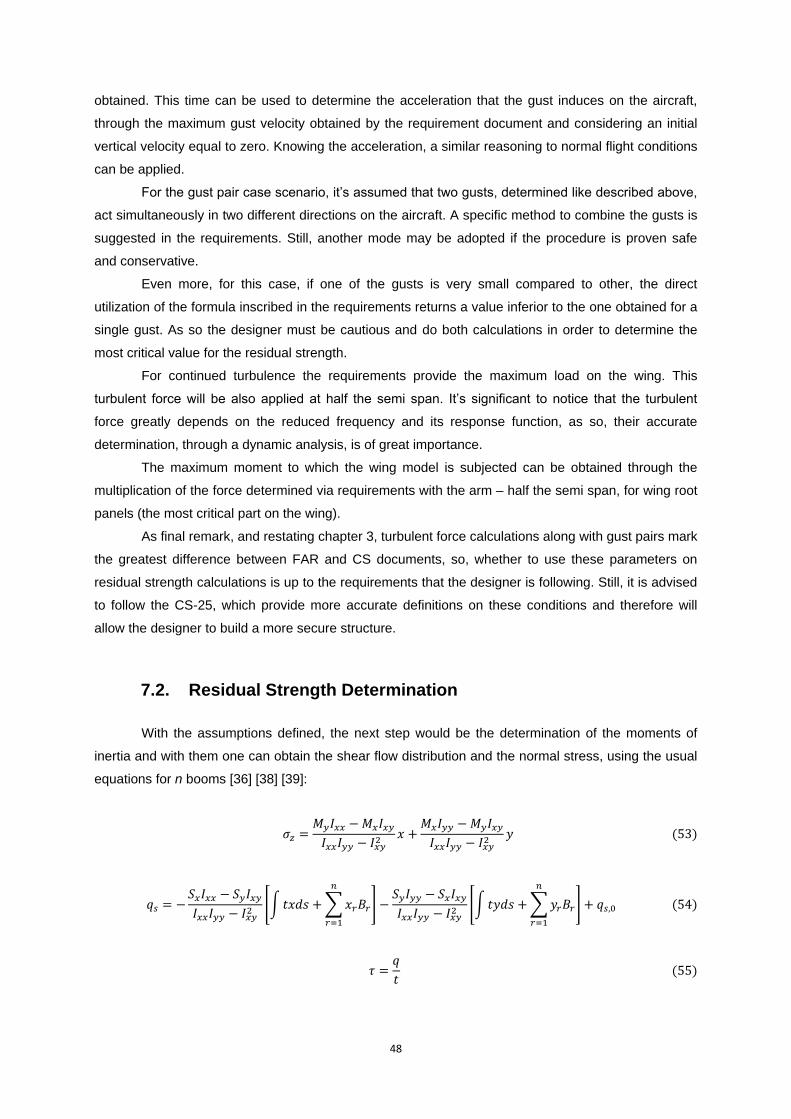
48
obtained. This time can be used to determine the acceleration that the gust induces on the aircraft,
through the maximum gust velocity obtained by the requirement document and considering an initial
vertical velocity equal to zero. Knowing the acceleration, a similar reasoning to normal flight conditions
can be applied.
For the gust pair case scenario, it‟s assumed that two gusts, determined like described above,
act simultaneously in two different directions on the aircraft. A specific method to combine the gusts is
suggested in the requirements. Still, another mode may be adopted if the procedure is proven safe
and conservative.
Even more, for this case, if one of the gusts is very small compared to other, the direct
utilization of the formula inscribed in the requirements returns a value inferior to the one obtained for a
single gust. As so the designer must be cautious and do both calculations in order to determine the
most critical value for the residual strength.
For continued turbulence the requirements provide the maximum load on the wing. This
turbulent force will be also applied at half the semi span. It‟s significant to notice that the turbulent
force greatly depends on the reduced frequency and its response function, as so, their accurate
determination, through a dynamic analysis, is of great importance.
The maximum moment to which the wing model is subjected can be obtained through the
multiplication of the force determined via requirements with the arm – half the semi span, for wing root
panels (the most critical part on the wing).
As final remark, and restating chapter 3, turbulent force calculations along with gust pairs mark
the greatest difference between FAR and CS documents, so, whether to use these parameters on
residual strength calculations is up to the requirements that the designer is following. Still, it is advised
to follow the CS-25, which provide more accurate definitions on these conditions and therefore will
allow the designer to build a more secure structure.
7.2. Residual Strength Determination
With the assumptions defined, the next step would be the determination of the moments of
inertia and with them one can obtain the shear flow distribution and the normal stress, using the usual
equations for n booms [36] [38] [39]:
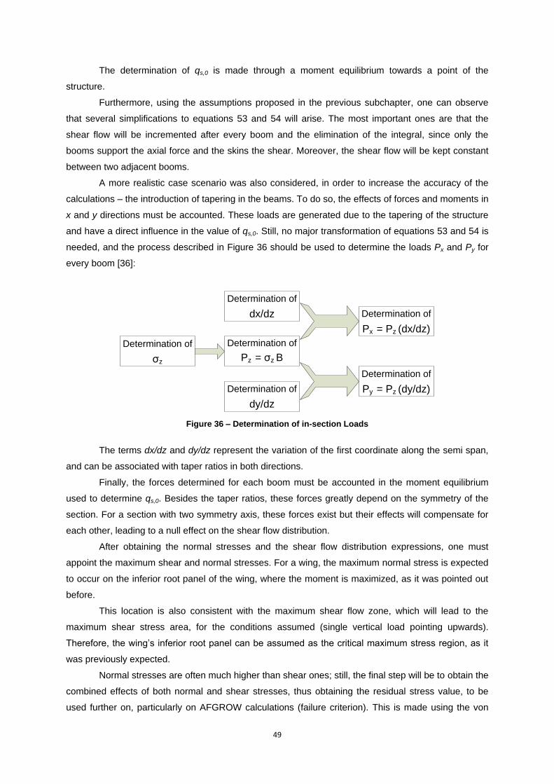
49
The determination of qs,0 is made through a moment equilibrium towards a point of the
structure.
Furthermore, using the assumptions proposed in the previous subchapter, one can observe
that several simplifications to equations 53 and 54 will arise. The most important ones are that the
shear flow will be incremented after every boom and the elimination of the integral, since only the
booms support the axial force and the skins the shear. Moreover, the shear flow will be kept constant
between two adjacent booms.
A more realistic case scenario was also considered, in order to increase the accuracy of the
calculations – the introduction of tapering in the beams. To do so, the effects of forces and moments in
x and y directions must be accounted. These loads are generated due to the tapering of the structure
and have a direct influence in the value of qs,0. Still, no major transformation of equations 53 and 54 is
needed, and the process described in Figure 36 should be used to determine the loads Px and Py for
every boom [36]:
Determination of
σz
Determination of
Pz = σz B
Determination of
dy/dz
Determination of
Py = Pz (dy/dz)
Determination of
Px = Pz (dx/dz)
Determination of
dx/dz
Figure 36 – Determination of in-section Loads
The terms dx/dz and dy/dz represent the variation of the first coordinate along the semi span,
and can be associated with taper ratios in both directions.
Finally, the forces determined for each boom must be accounted in the moment equilibrium
used to determine qs,0. Besides the taper ratios, these forces greatly depend on the symmetry of the
section. For a section with two symmetry axis, these forces exist but their effects will compensate for
each other, leading to a null effect on the shear flow distribution.
After obtaining the normal stresses and the shear flow distribution expressions, one must
appoint the maximum shear and normal stresses. For a wing, the maximum normal stress is expected
to occur on the inferior root panel of the wing, where the moment is maximized, as it was pointed out
before.
This location is also consistent with the maximum shear flow zone, which will lead to the
maximum shear stress area, for the conditions assumed (single vertical load pointing upwards).
Therefore, the wing‟s inferior root panel can be assumed as the critical maximum stress region, as it
was previously expected.
Normal stresses are often much higher than shear ones; still, the final step will be to obtain the
combined effects of both normal and shear stresses, thus obtaining the residual stress value, to be
used further on, particularly on AFGROW calculations (failure criterion). This is made using the von

50
Mises criterion, which states that [36]:
It is expected that a gust pair of maximum intensity or very strong continued turbulence define
the conditions for the most critical value for residual strength.
51
8. Crack Growth Analysis
The subjects addressed in this chapter were already defined and presented in chapter 2,
stress intensity factors and crack growth rates. Still, a much more detailed analysis as well as
determination procedures for these parameters will be conducted.
Furthermore, important characteristics already discussed in this thesis will now be gathered.
The highest stress concentration area will be chosen and the initial damage will be applied there, for
the residual strength value already stipulated.
The residual strength value along with KIC will define the most critical option that will lead to
component failure.
The definition of the crack growth rate through the stress intensity factor will enable the correct
determination of the number of cycles that a component can withstand until achieving a critical crack
length, thus allowing the design of a damage tolerant component. This can be observed in Figure 37.
Figure 37 – a) Cycles vs. Crack Growth; b) Stress Intensity Factor vs. Growth Rate [1]
There are two main paths to follow when determining the crack growth: an analytical
approach, based on the formulas already presented, or a computational approach, through software
like AFGROW or NASGRO.
8.1. Crack Retardation
Before defining the calculus for crack growth rate it is important to introduce the concept of
crack retardation. This phenomenon appears, most of the times, when an overload occurs. The
occurrence of overloads will create a greater plastic zone, like shown in Figure 38, which will slow
down crack progression due to residual compression stresses in the overload‟s plastic zone. This type
of phenomenon is very common and can lead to an increased number of cycles that a component can
withstand. [5]
a) b)
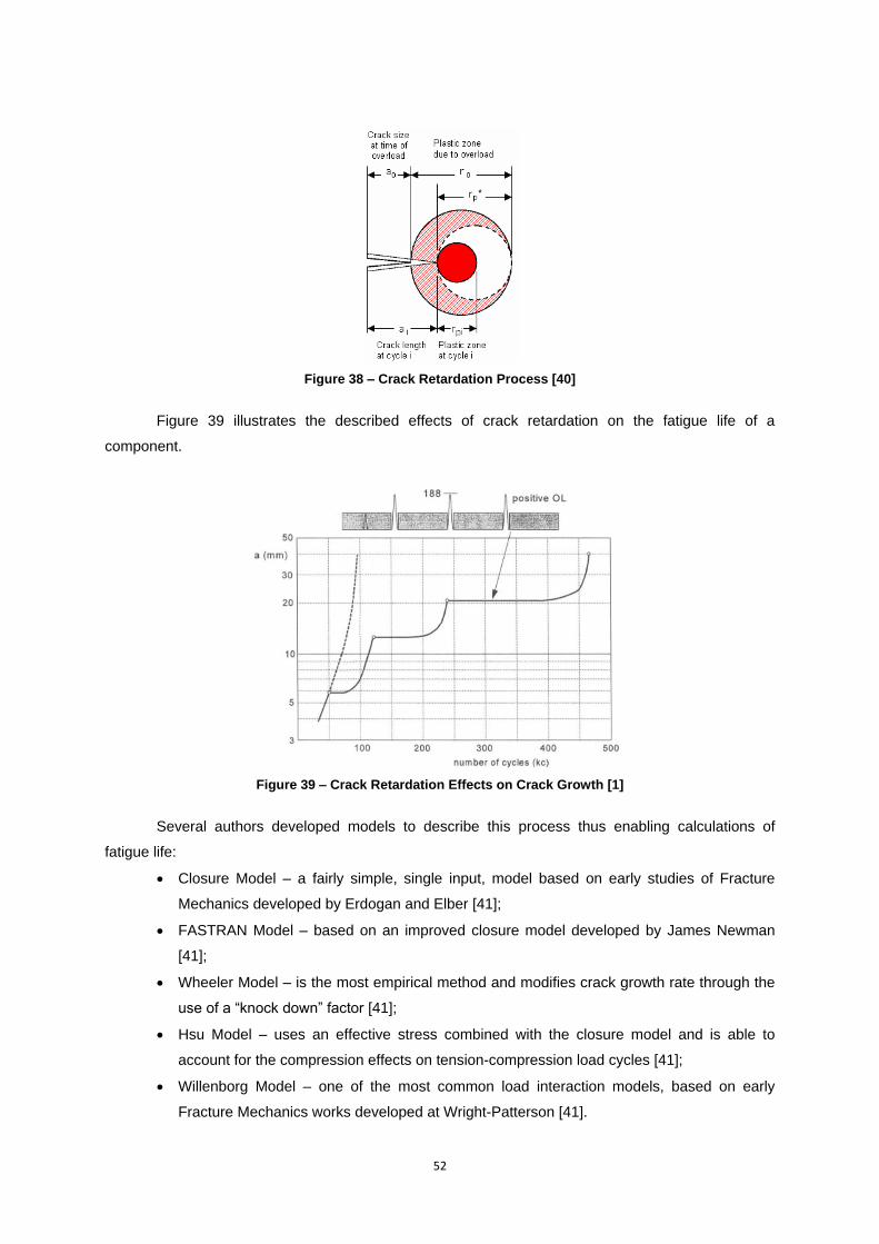
52
Figure 38 – Crack Retardation Process [40]
Figure 39 illustrates the described effects of crack retardation on the fatigue life of a
component.
Figure 39 – Crack Retardation Effects on Crack Growth [1]
Several authors developed models to describe this process thus enabling calculations of
fatigue life:
Closure Model – a fairly simple, single input, model based on early studies of Fracture
Mechanics developed by Erdogan and Elber [41];
FASTRAN Model – based on an improved closure model developed by James Newman
[41];
Wheeler Model – is the most empirical method and modifies crack growth rate through the
use of a “knock down” factor [41];
Hsu Model – uses an effective stress combined with the closure model and is able to
account for the compression effects on tension-compression load cycles [41];
Willenborg Model – one of the most common load interaction models, based on early
Fracture Mechanics works developed at Wright-Patterson [41].
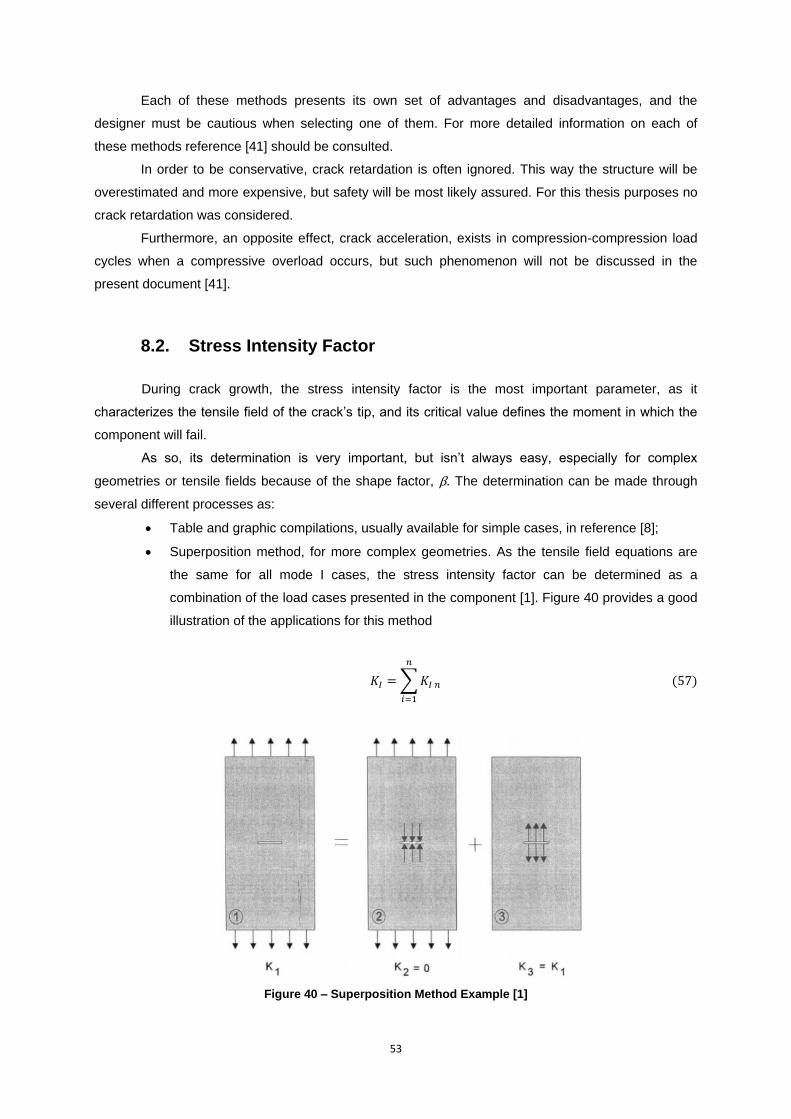
53
Each of these methods presents its own set of advantages and disadvantages, and the
designer must be cautious when selecting one of them. For more detailed information on each of
these methods reference [41] should be consulted.
In order to be conservative, crack retardation is often ignored. This way the structure will be
overestimated and more expensive, but safety will be most likely assured. For this thesis purposes no
crack retardation was considered.
Furthermore, an opposite effect, crack acceleration, exists in compression-compression load
cycles when a compressive overload occurs, but such phenomenon will not be discussed in the
present document [41].
8.2. Stress Intensity Factor
During crack growth, the stress intensity factor is the most important parameter, as it
characterizes the tensile field of the crack‟s tip, and its critical value defines the moment in which the
component will fail.
As so, its determination is very important, but isn‟t always easy, especially for complex
geometries or tensile fields because of the shape factor, β. The determination can be made through
several different processes as:
Table and graphic compilations, usually available for simple cases, in reference [8];
Superposition method, for more complex geometries. As the tensile field equations are
the same for all mode I cases, the stress intensity factor can be determined as a
combination of the load cases presented in the component [1]. Figure 40 provides a good
illustration of the applications for this method
Figure 40 – Superposition Method Example [1]
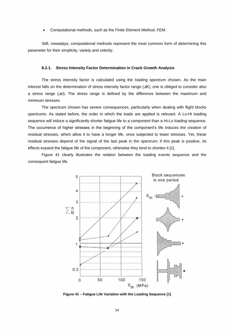
54
Computational methods, such as the Finite Element Method, FEM.
Still, nowadays, computational methods represent the most common form of determining this
parameter for their simplicity, variety and celerity.
8.2.1. Stress Intensity Factor Determination in Crack Growth Analysis
The stress intensity factor is calculated using the loading spectrum chosen. As the main
interest falls on the determination of stress intensity factor range (ΔK), one is obliged to consider also
a stress range (Δσ). The stress range is defined by the difference between the maximum and
minimum stresses.
The spectrum chosen has severe consequences, particularly when dealing with flight blocks
spectrums. As stated before, the order in which the loads are applied is relevant. A Lo-Hi loading
sequence will induce a significantly shorter fatigue life to a component than a Hi-Lo loading sequence.
The occurrence of higher stresses in the beginning of the component‟s life induces the creation of
residual stresses, which allow it to have a longer life, once subjected to lower stresses. Yet, these
residual stresses depend of the signal of the last peak in the spectrum; if this peak is positive, its
effects expand the fatigue life of the component, otherwise they tend to shorten it [1].
Figure 41 clearly illustrates the relation between the loading events sequence and the
consequent fatigue life.
Figure 41 – Fatigue Life Variation with the Loading Sequence [1]
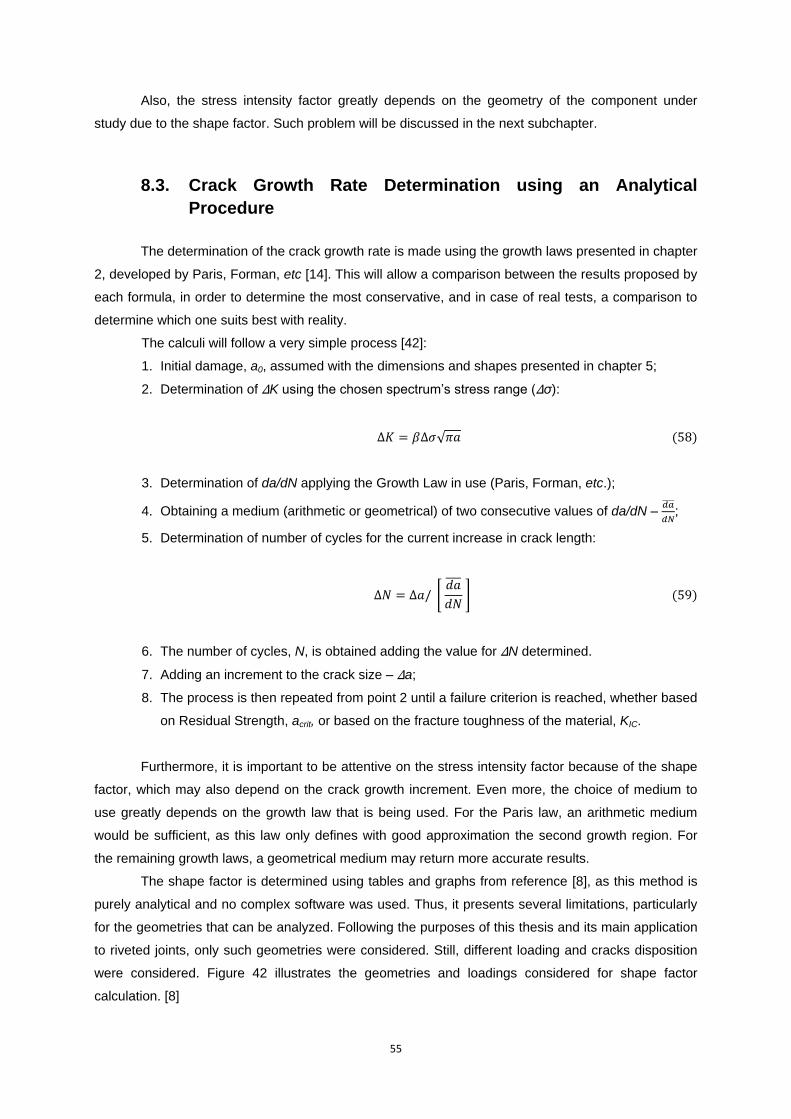
55
Also, the stress intensity factor greatly depends on the geometry of the component under
study due to the shape factor. Such problem will be discussed in the next subchapter.
8.3. Crack Growth Rate Determination using an Analytical
Procedure
The determination of the crack growth rate is made using the growth laws presented in chapter
2, developed by Paris, Forman, etc [14]. This will allow a comparison between the results proposed by
each formula, in order to determine the most conservative, and in case of real tests, a comparison to
determine which one suits best with reality.
The calculi will follow a very simple process [42]:
1. Initial damage, a0, assumed with the dimensions and shapes presented in chapter 5;
2. Determination of ΔK using the chosen spectrum‟s stress range (Δσ):
3. Determination of da/dN applying the Growth Law in use (Paris, Forman, etc.);
4. Obtaining a medium (arithmetic or geometrical) of two consecutive values of da/dN –
;
5. Determination of number of cycles for the current increase in crack length:
6. The number of cycles, N, is obtained adding the value for ΔN determined.
7. Adding an increment to the crack size – Δa;
8. The process is then repeated from point 2 until a failure criterion is reached, whether based
on Residual Strength, acrit, or based on the fracture toughness of the material, KIC.
Furthermore, it is important to be attentive on the stress intensity factor because of the shape
factor, which may also depend on the crack growth increment. Even more, the choice of medium to
use greatly depends on the growth law that is being used. For the Paris law, an arithmetic medium
would be sufficient, as this law only defines with good approximation the second growth region. For
the remaining growth laws, a geometrical medium may return more accurate results.
The shape factor is determined using tables and graphs from reference [8], as this method is
purely analytical and no complex software was used. Thus, it presents several limitations, particularly
for the geometries that can be analyzed. Following the purposes of this thesis and its main application
to riveted joints, only such geometries were considered. Still, different loading and cracks disposition
were considered. Figure 42 illustrates the geometries and loadings considered for shape factor
calculation. [8]
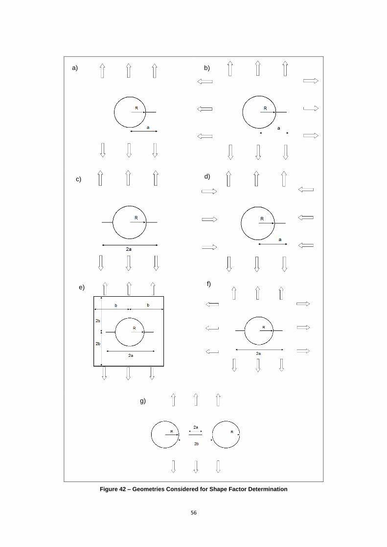
56
Figure 42 – Geometries Considered for Shape Factor Determination
a) b)
c) d)
e) f)
g)
57
Figure 42 illustrates the geometries and load configurations chosen. Only one of the
geometries considers a finite plate model, while others consider an infinite plate with remote applied
stresses (tension, compression or a combination of both).
Through this data, one is able to plot the two characteristic graphs for crack growth presented
before – number of cycles vs. crack length and stress intensity factor vs. crack growth rate, Figure 37.
Analyzing the two graphs, one can determine which law describes the process better, and make
comparisons between the several propagation models.
8.4. Crack Growth Rate Determination using AFGROW
In order to obtain the crack growth rate, without destructive testing, computer aided simulation
methods are often used. Using crack growth software, such as AFGROW or NASGRO, it is possible to
obtain the estimation to the fatigue life of the component. In some software, for more complex
geometries, there is the possibility of importing a finite element model, geometry and load disposition
into the crack growth software and make the estimation for the fatigue life of said part.
For this thesis purposes, AFGROW was the software chosen to be used, as it is freeware, has
an incorporated material database and possesses a tool that allows simple model‟s construction. This
software is one of most commonly used worldwide.
Software used for determining crack growth computes it through a similar procedure to one
presented in the previous subchapter. Furthermore, the software automatically determines the shape
factor and uses much more complex crack growth laws, but if necessary allows its manual introduction
for simple geometries, in table form.
One of the most used growth laws is the NASGRO Equation, which allows the introduction of
the higher number of constants, indicating that this law is expected to have the more accurate results.
As mentioned, the software already includes a material database, which contains the constants
needed for the NASGRO Equation growth law. Still, if the user needs to alter some parameters,
manual introduction is available [14] [41].
So the process to use for crack growth determination on AFGROW will follow these stages:
1. Introduction of the Geometry (model), whether user inputted or software incorporated (if
needed the shape factor table may be also inserted);
2. Crack Growth Law selection, usually NASGRO Equation for the reasons explained
previously. The component‟s material will be also selected in this step;
3. Introduction of a Retardation Model (by default no retardation is chosen leading to a more
conservative structure and its use is recurrent);
4. Spectrum insertion, with the definition of the Residual Strength value;
5. Run the software to determine the two plots (ΔK vs. da/dN and N vs. a).
It is very important to be cautious on spectrum selection, when the stress multiplication factor
is introduced. In AFGROW, the two spectrums are in percentage of different stresses – TWIST is in
percentage of the cruise flight stress and FALSTAFF is in percentage of the maximum stress.
Furthermore, if using the proposed normalized spectrums notice that they were built in percentage of

58
the cruise flight stress too.
Ten geometric models were created using the advanced model construction tool from
AFGROW. These models were created using standard hole, skin and crack sizes, which must be
altered to meet the problem conditions. Furthermore, steps 2 to 5 still must be conducted. Table 9
contains the models built.
a) Two holes and a central through crack
b) Two holes with a through crack on each one
c) Two holes with a corner crack on each one
d) Two holes with a through crack on one of them
e) Two holes with a corner crack on one of them
f) One hole with one through
crack
g) One hole with one corner
crack
h) One hole with two through
crack
i) One hole with one through
crack and one corner crack
j) One hole with two corner
crack
Table 9 – Geometric Models Built for Insertion on AFGROW
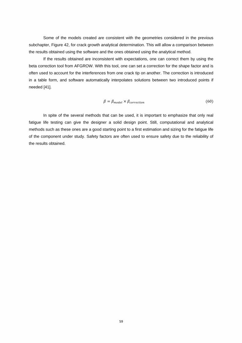
59
Some of the models created are consistent with the geometries considered in the previous
subchapter, Figure 42, for crack growth analytical determination. This will allow a comparison between
the results obtained using the software and the ones obtained using the analytical method.
If the results obtained are inconsistent with expectations, one can correct them by using the
beta correction tool from AFGROW. With this tool, one can set a correction for the shape factor and is
often used to account for the interferences from one crack tip on another. The correction is introduced
in a table form, and software automatically interpolates solutions between two introduced points if
needed [41].
In spite of the several methods that can be used, it is important to emphasize that only real
fatigue life testing can give the designer a solid design point. Still, computational and analytical
methods such as these ones are a good starting point to a first estimation and sizing for the fatigue life
of the component under study. Safety factors are often used to ensure safety due to the reliability of
the results obtained.

60
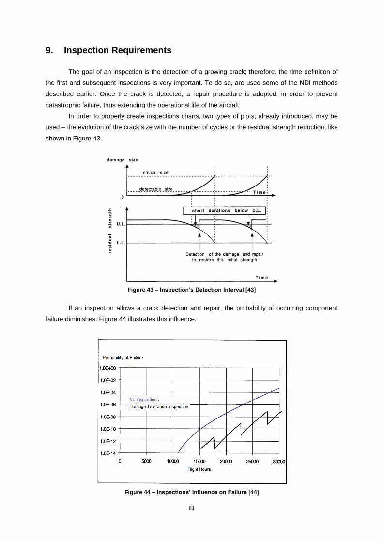
61
9. Inspection Requirements
The goal of an inspection is the detection of a growing crack; therefore, the time definition of
the first and subsequent inspections is very important. To do so, are used some of the NDI methods
described earlier. Once the crack is detected, a repair procedure is adopted, in order to prevent
catastrophic failure, thus extending the operational life of the aircraft.
In order to properly create inspections charts, two types of plots, already introduced, may be
used – the evolution of the crack size with the number of cycles or the residual strength reduction, like
shown in Figure 43.
Figure 43 – Inspection’s Detection Interval [43]
If an inspection allows a crack detection and repair, the probability of occurring component
failure diminishes. Figure 44 illustrates this influence.
Figure 44 – Inspections’ Influence on Failure [44]
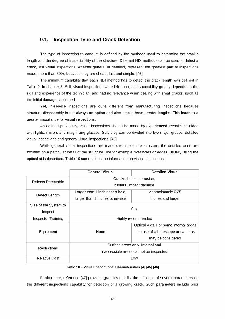
62
9.1. Inspection Type and Crack Detection
The type of inspection to conduct is defined by the methods used to determine the crack‟s
length and the degree of inspectability of the structure. Different NDI methods can be used to detect a
crack, still visual inspections, whether general or detailed, represent the greatest part of inspections
made, more than 80%, because they are cheap, fast and simple. [45]
The minimum capability that each NDI method has to detect the crack length was defined in
Table 2, in chapter 5. Still, visual inspections were left apart, as its capability greatly depends on the
skill and experience of the technician, and had no relevance when dealing with small cracks, such as
the initial damages assumed.
Yet, in-service inspections are quite different from manufacturing inspections because
structure disassembly is not always an option and also cracks have greater lengths. This leads to a
greater importance for visual inspections.
As defined previously, visual inspections should be made by experienced technicians aided
with lights, mirrors and magnifying glasses. Still, they can be divided into two major groups: detailed
visual inspections and general visual inspections. [46]
While general visual inspections are made over the entire structure, the detailed ones are
focused on a particular detail of the structure, like for example rivet holes or edges, usually using the
optical aids described. Table 10 summarizes the information on visual inspections:
General Visual Detailed Visual
Defects Detectable Cracks, holes, corrosion,
blisters, impact damage
Defect Length Larger than 1 inch near a hole,
larger than 2 inches otherwise
Approximately 0.25
inches and larger
Size of the System to
Inspect Any
Inspector Training Highly recommended
Equipment None
Optical Aids. For some internal areas
the use of a borescope or cameras
may be considered
Restrictions Surface areas only. Internal and
inaccessible areas cannot be inspected
Relative Cost Low
Table 10 – Visual Inspections’ Characteristics [4] [45] [46]
Furthermore, reference [47] provides graphics that list the influence of several parameters on
the different inspections capability for detection of a growing crack. Such parameters include prior
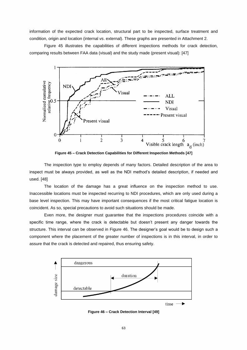
63
information of the expected crack location, structural part to be inspected, surface treatment and
condition, origin and location (internal vs. external). These graphs are presented in Attachment 2.
Figure 45 illustrates the capabilities of different inspections methods for crack detection,
comparing results between FAA data (visual) and the study made (present visual): [47]
Figure 45 – Crack Detection Capabilities for Different Inspection Methods [47]
The inspection type to employ depends of many factors. Detailed description of the area to
inspect must be always provided, as well as the NDI method‟s detailed description, if needed and
used. [48]
The location of the damage has a great influence on the inspection method to use.
Inaccessible locations must be inspected recurring to NDI procedures, which are only used during a
base level inspection. This may have important consequences if the most critical fatigue location is
coincident. As so, special precautions to avoid such situations should be made.
Even more, the designer must guarantee that the inspections procedures coincide with a
specific time range, where the crack is detectable but doesn‟t present any danger towards the
structure. This interval can be observed in Figure 46. The designer‟s goal would be to design such a
component where the placement of the greater number of inspections is in this interval, in order to
assure that the crack is detected and repaired, thus ensuring safety.
Figure 46 – Crack Detection Interval [49]
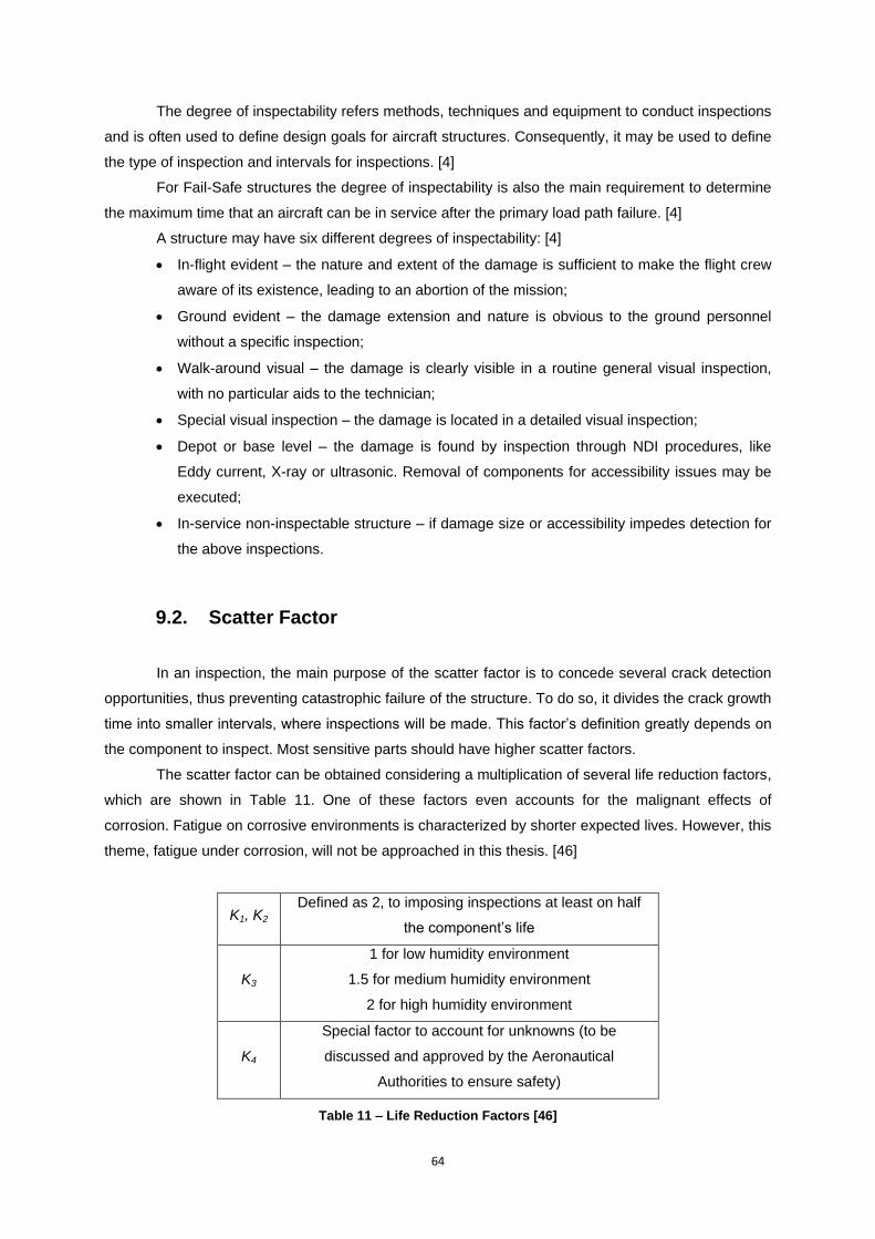
64
The degree of inspectability refers methods, techniques and equipment to conduct inspections
and is often used to define design goals for aircraft structures. Consequently, it may be used to define
the type of inspection and intervals for inspections. [4]
For Fail-Safe structures the degree of inspectability is also the main requirement to determine
the maximum time that an aircraft can be in service after the primary load path failure. [4]
A structure may have six different degrees of inspectability: [4]
In-flight evident – the nature and extent of the damage is sufficient to make the flight crew
aware of its existence, leading to an abortion of the mission;
Ground evident – the damage extension and nature is obvious to the ground personnel
without a specific inspection;
Walk-around visual – the damage is clearly visible in a routine general visual inspection,
with no particular aids to the technician;
Special visual inspection – the damage is located in a detailed visual inspection;
Depot or base level – the damage is found by inspection through NDI procedures, like
Eddy current, X-ray or ultrasonic. Removal of components for accessibility issues may be
executed;
In-service non-inspectable structure – if damage size or accessibility impedes detection for
the above inspections.
9.2. Scatter Factor
In an inspection, the main purpose of the scatter factor is to concede several crack detection
opportunities, thus preventing catastrophic failure of the structure. To do so, it divides the crack growth
time into smaller intervals, where inspections will be made. This factor‟s definition greatly depends on
the component to inspect. Most sensitive parts should have higher scatter factors.
The scatter factor can be obtained considering a multiplication of several life reduction factors,
which are shown in Table 11. One of these factors even accounts for the malignant effects of
corrosion. Fatigue on corrosive environments is characterized by shorter expected lives. However, this
theme, fatigue under corrosion, will not be approached in this thesis. [46]
K1, K2 Defined as 2, to imposing inspections at least on half
the component‟s life
K3
1 for low humidity environment
1.5 for medium humidity environment
2 for high humidity environment
K4
Special factor to account for unknowns (to be
discussed and approved by the Aeronautical
Authorities to ensure safety)
Table 11 – Life Reduction Factors [46]
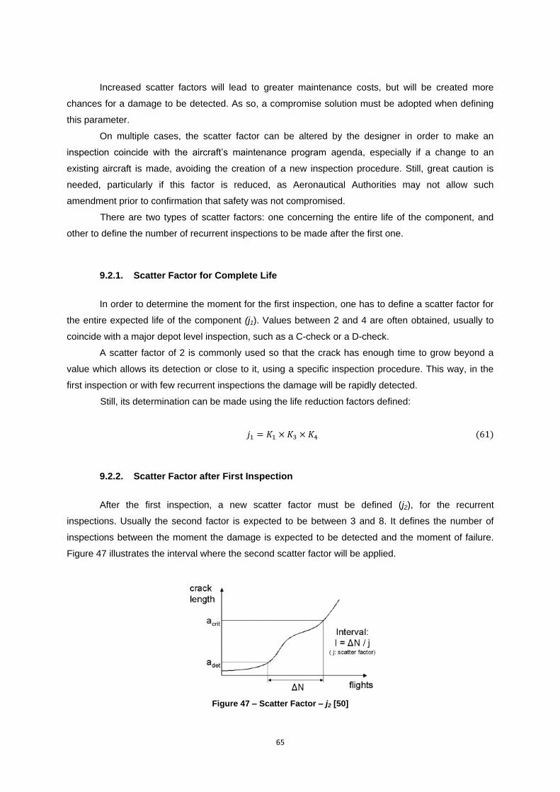
65
Increased scatter factors will lead to greater maintenance costs, but will be created more
chances for a damage to be detected. As so, a compromise solution must be adopted when defining
this parameter.
On multiple cases, the scatter factor can be altered by the designer in order to make an
inspection coincide with the aircraft‟s maintenance program agenda, especially if a change to an
existing aircraft is made, avoiding the creation of a new inspection procedure. Still, great caution is
needed, particularly if this factor is reduced, as Aeronautical Authorities may not allow such
amendment prior to confirmation that safety was not compromised.
There are two types of scatter factors: one concerning the entire life of the component, and
other to define the number of recurrent inspections to be made after the first one.
9.2.1. Scatter Factor for Complete Life
In order to determine the moment for the first inspection, one has to define a scatter factor for
the entire expected life of the component (j1). Values between 2 and 4 are often obtained, usually to
coincide with a major depot level inspection, such as a C-check or a D-check.
A scatter factor of 2 is commonly used so that the crack has enough time to grow beyond a
value which allows its detection or close to it, using a specific inspection procedure. This way, in the
first inspection or with few recurrent inspections the damage will be rapidly detected.
Still, its determination can be made using the life reduction factors defined:
9.2.2. Scatter Factor after First Inspection
After the first inspection, a new scatter factor must be defined (j2), for the recurrent
inspections. Usually the second factor is expected to be between 3 and 8. It defines the number of
inspections between the moment the damage is expected to be detected and the moment of failure.
Figure 47 illustrates the interval where the second scatter factor will be applied.
Figure 47 – Scatter Factor – j2 [50]
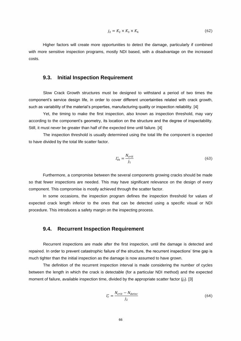
66
Higher factors will create more opportunities to detect the damage, particularly if combined
with more sensitive inspection programs, mostly NDI based, with a disadvantage on the increased
costs.
9.3. Initial Inspection Requirement
Slow Crack Growth structures must be designed to withstand a period of two times the
component‟s service design life, in order to cover different uncertainties related with crack growth,
such as variability of the material‟s properties, manufacturing quality or inspection reliability. [4]
Yet, the timing to make the first inspection, also known as inspection threshold, may vary
according to the component‟s geometry, its location on the structure and the degree of inspectability.
Still, it must never be greater than half of the expected time until failure. [4]
The inspection threshold is usually determined using the total life the component is expected
to have divided by the total life scatter factor.
Furthermore, a compromise between the several components growing cracks should be made
so that fewer inspections are needed. This may have significant relevance on the design of every
component. This compromise is mostly achieved through the scatter factor.
In some occasions, the inspection program defines the inspection threshold for values of
expected crack length inferior to the ones that can be detected using a specific visual or NDI
procedure. This introduces a safety margin on the inspecting process.
9.4. Recurrent Inspection Requirement
Recurrent inspections are made after the first inspection, until the damage is detected and
repaired. In order to prevent catastrophic failure of the structure, the recurrent inspections‟ time gap is
much tighter than the initial inspection as the damage is now assumed to have grown.
The definition of the recurrent inspection interval is made considering the number of cycles
between the length in which the crack is detectable (for a particular NDI method) and the expected
moment of failure, available inspection time, divided by the appropriate scatter factor (j2). [3]
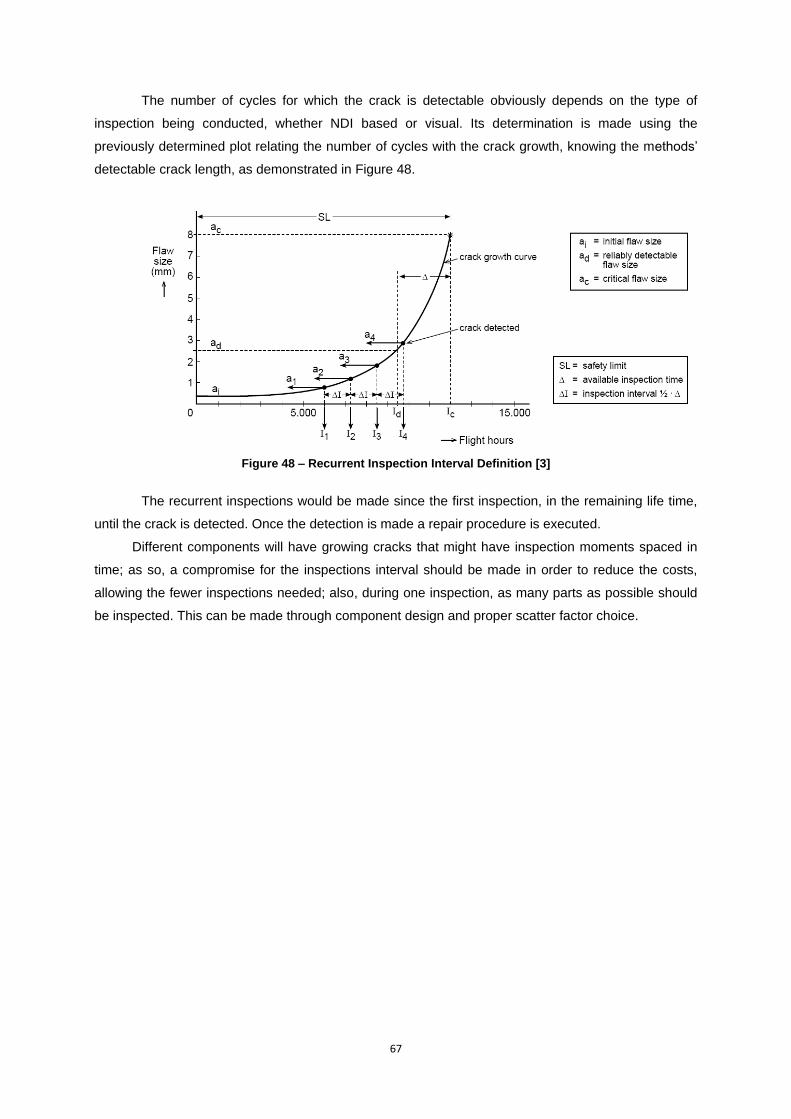
67
The number of cycles for which the crack is detectable obviously depends on the type of
inspection being conducted, whether NDI based or visual. Its determination is made using the
previously determined plot relating the number of cycles with the crack growth, knowing the methods‟
detectable crack length, as demonstrated in Figure 48.
Figure 48 – Recurrent Inspection Interval Definition [3]
The recurrent inspections would be made since the first inspection, in the remaining life time,
until the crack is detected. Once the detection is made a repair procedure is executed.
Different components will have growing cracks that might have inspection moments spaced in
time; as so, a compromise for the inspections interval should be made in order to reduce the costs,
allowing the fewer inspections needed; also, during one inspection, as many parts as possible should
be inspected. This can be made through component design and proper scatter factor choice.

68

69
10. Example of a Damage Tolerance Analysis of a Wing Panel
In this chapter will be conducted a study to determine the damage tolerance capabilities of a
repair made on a lower wing panel, following the procedure developed, together with the Excel files
and AFGROW models created.
The wing under study belongs to a Lockheed C-130A, with an internal structure, as presented
in Figure 49. Three damaged locations were considered in the highlighted panel (see Figure 50): one
on the root, other on the mid semi span and another at the wing tip. This panel is a machinated semi
span long panel, with non linear variable thickness, built in aluminium alloy 7075-T6.
Figure 49 – Structure of the Lockheed C-130A Wing
Figure 50 – Scheme for the Analyzed Wing (without Externally Mounted Probes)
For the damages considered near the wing root and tip, two different approaches can be
made: either considering 10 inches towards the margin or that the damage starts in the margin. The
following calculations were done considering the 10 inches margin.
Stress concentration is not an issue for this example once the panel doesn‟t contain any
fastener holes or particular geometrical feature that would introduce such concentration. Still, the
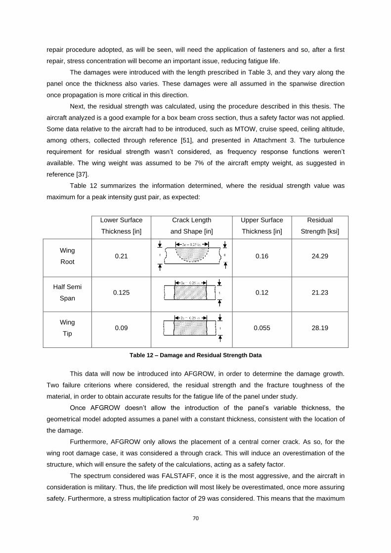
70
repair procedure adopted, as will be seen, will need the application of fasteners and so, after a first
repair, stress concentration will become an important issue, reducing fatigue life.
The damages were introduced with the length prescribed in Table 3, and they vary along the
panel once the thickness also varies. These damages were all assumed in the spanwise direction
once propagation is more critical in this direction.
Next, the residual strength was calculated, using the procedure described in this thesis. The
aircraft analyzed is a good example for a box beam cross section, thus a safety factor was not applied.
Some data relative to the aircraft had to be introduced, such as MTOW, cruise speed, ceiling altitude,
among others, collected through reference [51], and presented in Attachment 3. The turbulence
requirement for residual strength wasn‟t considered, as frequency response functions weren‟t
available. The wing weight was assumed to be 7% of the aircraft empty weight, as suggested in
reference [37].
Table 12 summarizes the information determined, where the residual strength value was
maximum for a peak intensity gust pair, as expected:
Lower Surface
Thickness [in]
Crack Length
and Shape [in]
Upper Surface
Thickness [in]
Residual
Strength [ksi]
Wing
Root 0.21
0.16 24.29
Half Semi
Span 0.125
0.12 21.23
Wing
Tip 0.09
0.055 28.19
Table 12 – Damage and Residual Strength Data
This data will now be introduced into AFGROW, in order to determine the damage growth.
Two failure criterions where considered, the residual strength and the fracture toughness of the
material, in order to obtain accurate results for the fatigue life of the panel under study.
Once AFGROW doesn‟t allow the introduction of the panel‟s variable thickness, the
geometrical model adopted assumes a panel with a constant thickness, consistent with the location of
the damage.
Furthermore, AFGROW only allows the placement of a central corner crack. As so, for the
wing root damage case, it was considered a through crack. This will induce an overestimation of the
structure, which will ensure the safety of the calculations, acting as a safety factor.
The spectrum considered was FALSTAFF, once it is the most aggressive, and the aircraft in
consideration is military. Thus, the life prediction will most likely be overestimated, once more assuring
safety. Furthermore, a stress multiplication factor of 29 was considered. This means that the maximum
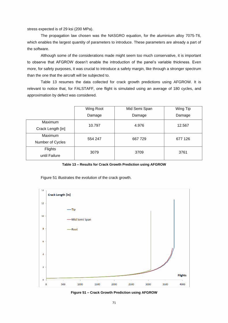
71
stress expected is of 29 ksi (200 MPa).
The propagation law chosen was the NASGRO equation, for the aluminium alloy 7075-T6,
which enables the largest quantity of parameters to introduce. These parameters are already a part of
the software.
Although some of the considerations made might seem too much conservative, it is important
to observe that AFGROW doesn‟t enable the introduction of the panel‟s variable thickness. Even
more, for safety purposes, it was crucial to introduce a safety margin, like through a stronger spectrum
than the one that the aircraft will be subjected to.
Table 13 resumes the data collected for crack growth predictions using AFGROW. It is
relevant to notice that, for FALSTAFF, one flight is simulated using an average of 180 cycles, and
approximation by defect was considered.
Wing Root
Damage
Mid Semi Span
Damage
Wing Tip
Damage
Maximum
Crack Length [in] 10.797 4.976 12.567
Maximum
Number of Cycles 554 247 667 729 677 126
Flights
until Failure 3079 3709 3761
Table 13 – Results for Crack Growth Prediction using AFGROW
Figure 51 illustrates the evolution of the crack growth.
Figure 51 – Crack Growth Prediction using AFGROW
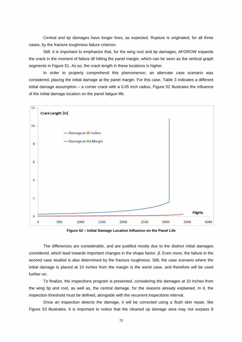
72
Central and tip damages have longer lives, as expected. Rupture is originated, for all three
cases, by the fracture toughness failure criterion.
Still, it is important to emphasize that, for the wing root and tip damages, AFGROW expands
the crack in the moment of failure till hitting the panel margin, which can be seen as the vertical graph
segments in Figure 51. As so, the crack length in these locations is higher.
In order to properly comprehend this phenomenon, an alternate case scenario was
considered, placing the initial damage at the panel margin. For this case, Table 3 indicates a different
initial damage assumption – a corner crack with a 0.05 inch radius. Figure 52 illustrates the influence
of the initial damage location on the panel fatigue life.
Figure 52 – Initial Damage Location Influence on the Panel Life
The differences are considerable, and are justified mostly due to the distinct initial damages
considered, which lead towards important changes in the shape factor, β. Even more, the failure in the
second case studied is also determined by the fracture toughness. Still, the case scenario where the
initial damage is placed at 10 inches from the margin is the worst case, and therefore will be used
further on.
To finalize, the inspections program is presented, considering the damages at 10 inches from
the wing tip and root, as well as, the central damage, for the reasons already explained. In it, the
inspection threshold must be defined, alongside with the recurrent inspections interval.
Once an inspection detects the damage, it will be corrected using a flush skin repair, like
Figure 53 illustrates. It is important to notice that the cleaned up damage area may not surpass 8
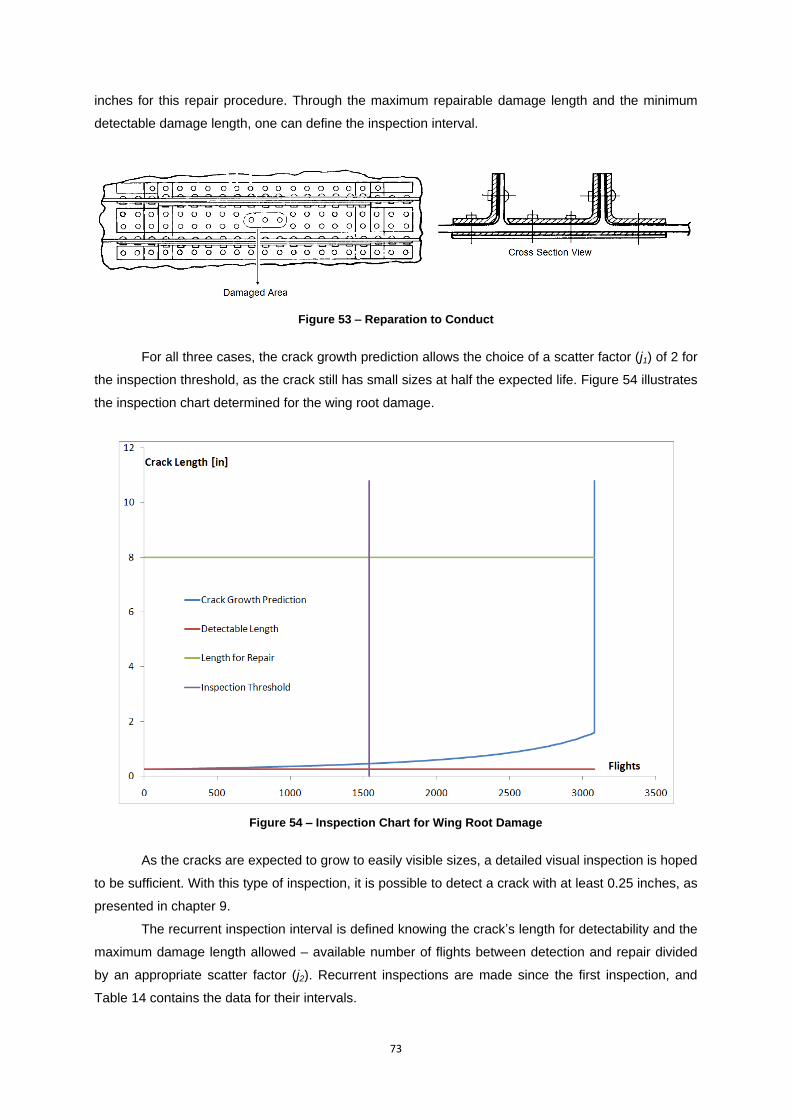
73
inches for this repair procedure. Through the maximum repairable damage length and the minimum
detectable damage length, one can define the inspection interval.
Figure 53 – Reparation to Conduct
For all three cases, the crack growth prediction allows the choice of a scatter factor (j1) of 2 for
the inspection threshold, as the crack still has small sizes at half the expected life. Figure 54 illustrates
the inspection chart determined for the wing root damage.
Figure 54 – Inspection Chart for Wing Root Damage
As the cracks are expected to grow to easily visible sizes, a detailed visual inspection is hoped
to be sufficient. With this type of inspection, it is possible to detect a crack with at least 0.25 inches, as
presented in chapter 9.
The recurrent inspection interval is defined knowing the crack‟s length for detectability and the
maximum damage length allowed – available number of flights between detection and repair divided
by an appropriate scatter factor (j2). Recurrent inspections are made since the first inspection, and
Table 14 contains the data for their intervals.
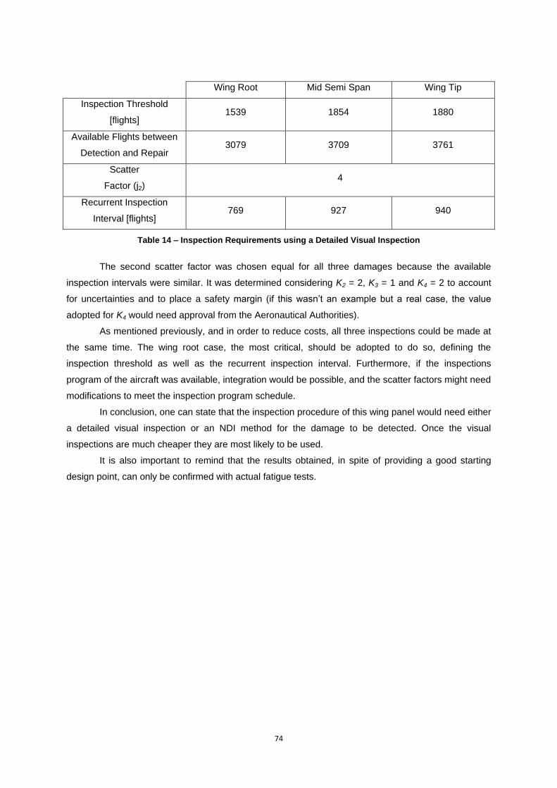
74
Wing Root Mid Semi Span Wing Tip
Inspection Threshold
[flights] 1539 1854 1880
Available Flights between
Detection and Repair 3079 3709 3761
Scatter
Factor (j2) 4
Recurrent Inspection
Interval [flights] 769 927 940
Table 14 – Inspection Requirements using a Detailed Visual Inspection
The second scatter factor was chosen equal for all three damages because the available
inspection intervals were similar. It was determined considering K2 = 2, K3 = 1 and K4 = 2 to account
for uncertainties and to place a safety margin (if this wasn‟t an example but a real case, the value
adopted for K4 would need approval from the Aeronautical Authorities).
As mentioned previously, and in order to reduce costs, all three inspections could be made at
the same time. The wing root case, the most critical, should be adopted to do so, defining the
inspection threshold as well as the recurrent inspection interval. Furthermore, if the inspections
program of the aircraft was available, integration would be possible, and the scatter factors might need
modifications to meet the inspection program schedule.
In conclusion, one can state that the inspection procedure of this wing panel would need either
a detailed visual inspection or an NDI method for the damage to be detected. Once the visual
inspections are much cheaper they are most likely to be used.
It is also important to remind that the results obtained, in spite of providing a good starting
design point, can only be confirmed with actual fatigue tests.
75
11. Concluding Remarks and Future Developments
Damage Tolerance Design analysis of structures is an everyday procedure for maintenance
companies all over the world. As so, this thesis contains a standardized procedure to make
estimations on damage tolerance of a structure as thus promoting more accurate inspection timing,
which will ultimately lead to smaller costs for the company.
Damage tolerance is estimated over several steps:
1. Determination of the most critical point in terms of stress concentration (crack initiation and
propagation is easier at these locations);
2. Definition of the initial damage (length, direction, shape and quantity);
3. Definition of the spectrum to use, whether from a real aircraft or algorithm based, usually
selected concerning the type of aircraft that is being analysed;
4. Residual strength limits, calculated from the Airworthiness Requirements, defining the
maximum allowed crack length on the structure;
5. Crack growth determination will enable to compute the number of cycles for the structure to
have grown a crack with a prescribed dimension;
6. Inspection procedure definition, emphasizing the definition of the inspection threshold and
inspection interval. The construction of the inspection charts is made through these
parameters.
When these steps are completed, and a Damage Tolerance Analysis has been conducted, the
following must be provided:
The residual strength as a function of the crack size;
The crack growth, emphasizing the number of cycles till failure and critical crack length;
The initial damage assumed;
The inspection interval.
Future developments should be concerned with the introduction of more accurate methods to
determine residual strength and crack growth rate, for which several simplifications were made in the
interest of aiding the calculations. Also, in the interest of obtaining more accurate calculations, in-flight
spectrums of the aircraft analysed should be used. This will allow a reduction of the overestimation of
the structures thus reducing costs.
The methods used to determine stress concentration, calculate the fastener constant using
Tom Swift‟s formula. Yet, other formulas, more precise and accurate, exist. The development of such
formulas will allow the designers not to build overestimated structures.
AFGROW provides acceptable results, but its use should be made with special attention, as
only real fatigue testing can accurately estimate the fatigue life. Even more, the software doesn‟t allow
the introduction of more than two cracks, which may lead to the utilization of other software, that isn‟t
freeware, such as NASGRO. Nevertheless the software AFGROW provides a good and reliable
starting point.
Procedures that allow a more accurate determination for the inspection threshold and inspection interval may be considered.

76
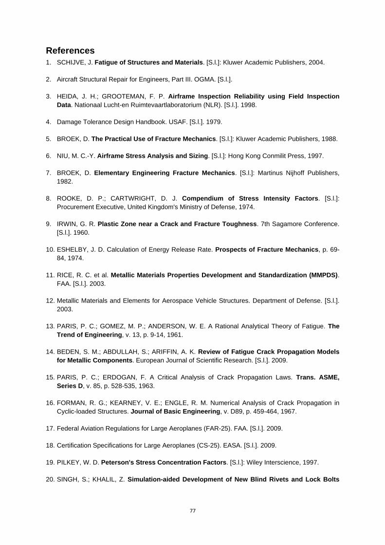
77
References
1. SCHIJVE, J. Fatigue of Structures and Materials. [S.l.]: Kluwer Academic Publishers, 2004.
2. Aircraft Structural Repair for Engineers, Part III. OGMA. [S.l.].
3. HEIDA, J. H.; GROOTEMAN, F. P. Airframe Inspection Reliability using Field Inspection
Data. Nationaal Lucht-en Ruimtevaartlaboratorium (NLR). [S.l.]. 1998.
4. Damage Tolerance Design Handbook. USAF. [S.l.]. 1979.
5. BROEK, D. The Practical Use of Fracture Mechanics. [S.l.]: Kluwer Academic Publishers, 1988.
6. NIU, M. C.-Y. Airframe Stress Analysis and Sizing. [S.l.]: Hong Kong Conmilit Press, 1997.
7. BROEK, D. Elementary Engineering Fracture Mechanics. [S.l.]: Martinus Nijhoff Publishers,
1982.
8. ROOKE, D. P.; CARTWRIGHT, D. J. Compendium of Stress Intensity Factors. [S.l.]:
Procurement Executive, United Kingdom's Ministry of Defense, 1974.
9. IRWIN, G. R. Plastic Zone near a Crack and Fracture Toughness. 7th Sagamore Conference.
[S.l.]. 1960.
10. ESHELBY, J. D. Calculation of Energy Release Rate. Prospects of Fracture Mechanics, p. 69-
84, 1974.
11. RICE, R. C. et al. Metallic Materials Properties Development and Standardization (MMPDS).
FAA. [S.l.]. 2003.
12. Metallic Materials and Elements for Aerospace Vehicle Structures. Department of Defense. [S.l.].
2003.
13. PARIS, P. C.; GOMEZ, M. P.; ANDERSON, W. E. A Rational Analytical Theory of Fatigue. The
Trend of Engineering, v. 13, p. 9-14, 1961.
14. BEDEN, S. M.; ABDULLAH, S.; ARIFFIN, A. K. Review of Fatigue Crack Propagation Models
for Metallic Components. European Journal of Scientific Research. [S.l.]. 2009.
15. PARIS, P. C.; ERDOGAN, F. A Critical Analysis of Crack Propagation Laws. Trans. ASME,
Series D, v. 85, p. 528-535, 1963.
16. FORMAN, R. G.; KEARNEY, V. E.; ENGLE, R. M. Numerical Analysis of Crack Propagation in
Cyclic-loaded Structures. Journal of Basic Engineering, v. D89, p. 459-464, 1967.
17. Federal Aviation Regulations for Large Aeroplanes (FAR-25). FAA. [S.l.]. 2009.
18. Certification Specifications for Large Aeroplanes (CS-25). EASA. [S.l.]. 2009.
19. PILKEY, W. D. Peterson's Stress Concentration Factors. [S.l.]: Wiley Interscience, 1997.
20. SINGH, S.; KHALIL, Z. Simulation-aided Development of New Blind Rivets and Lock Bolts
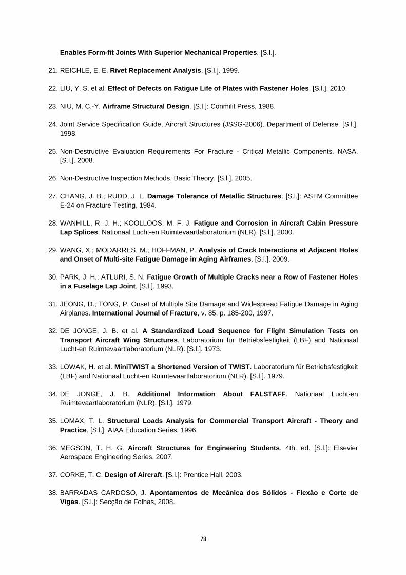
78
Enables Form-fit Joints With Superior Mechanical Properties. [S.l.].
21. REICHLE, E. E. Rivet Replacement Analysis. [S.l.]. 1999.
22. LIU, Y. S. et al. Effect of Defects on Fatigue Life of Plates with Fastener Holes. [S.l.]. 2010.
23. NIU, M. C.-Y. Airframe Structural Design. [S.l.]: Conmilit Press, 1988.
24. Joint Service Specification Guide, Aircraft Structures (JSSG-2006). Department of Defense. [S.l.].
1998.
25. Non-Destructive Evaluation Requirements For Fracture - Critical Metallic Components. NASA.
[S.l.]. 2008.
26. Non-Destructive Inspection Methods, Basic Theory. [S.l.]. 2005.
27. CHANG, J. B.; RUDD, J. L. Damage Tolerance of Metallic Structures. [S.l.]: ASTM Committee
E-24 on Fracture Testing, 1984.
28. WANHILL, R. J. H.; KOOLLOOS, M. F. J. Fatigue and Corrosion in Aircraft Cabin Pressure
Lap Splices. Nationaal Lucht-en Ruimtevaartlaboratorium (NLR). [S.l.]. 2000.
29. WANG, X.; MODARRES, M.; HOFFMAN, P. Analysis of Crack Interactions at Adjacent Holes
and Onset of Multi-site Fatigue Damage in Aging Airframes. [S.l.]. 2009.
30. PARK, J. H.; ATLURI, S. N. Fatigue Growth of Multiple Cracks near a Row of Fastener Holes
in a Fuselage Lap Joint. [S.l.]. 1993.
31. JEONG, D.; TONG, P. Onset of Multiple Site Damage and Widespread Fatigue Damage in Aging
Airplanes. International Journal of Fracture, v. 85, p. 185-200, 1997.
32. DE JONGE, J. B. et al. A Standardized Load Sequence for Flight Simulation Tests on
Transport Aircraft Wing Structures. Laboratorium für Betriebsfestigkeit (LBF) and Nationaal
Lucht-en Ruimtevaartlaboratorium (NLR). [S.l.]. 1973.
33. LOWAK, H. et al. MiniTWIST a Shortened Version of TWIST. Laboratorium für Betriebsfestigkeit
(LBF) and Nationaal Lucht-en Ruimtevaartlaboratorium (NLR). [S.l.]. 1979.
34. DE JONGE, J. B. Additional Information About FALSTAFF. Nationaal Lucht-en
Ruimtevaartlaboratorium (NLR). [S.l.]. 1979.
35. LOMAX, T. L. Structural Loads Analysis for Commercial Transport Aircraft - Theory and
Practice. [S.l.]: AIAA Education Series, 1996.
36. MEGSON, T. H. G. Aircraft Structures for Engineering Students. 4th. ed. [S.l.]: Elsevier
Aerospace Engineering Series, 2007.
37. CORKE, T. C. Design of Aircraft. [S.l.]: Prentice Hall, 2003.
38. BARRADAS CARDOSO, J. Apontamentos de Mecânica dos Sólidos - Flexão e Corte de
Vigas. [S.l.]: Secção de Folhas, 2008.
79
39. YOUNG, W. C.; BUDYNAS, R. G. Roark's Formulas for Stress and Strain. 7th. ed. [S.l.]:
McGraw-Hill, 2002.
40. Engrasp - Worldwide Engineering Solutions. Available at: <http://www.engrasp.com/
doc/etb/mod/fm1/paris/Figure06a.gif>. Acessed in: August 2010.
41. AFGROW Manual. [S.l.]. 2007.
42. ZHANG, X. Aircraft Fatigue and Damage Tolerance. [S.l.]: Cranfield University - College of
Aeronautics, 2002.
43. VAN BEIJNEN, M. N. et al. Damage Tolerance Aspects of a Full Composite Airplane
Fuselage. Delft University of Technology. [S.l.]. 1993.
44. LINCOLN, J. W. Role of Non-destructive Inspections in Airworthiness Assurance. USAF.
[S.l.]. 1998.
45. MATZKANIN, G. A. Selecting a Non-destructive Testing Method, Part II: Visual Inspection.
AMMTIAC Quarterly - Tech Solution 2, v. 1.
46. Approval Procedures For Modifications and Repairs to Damage Tolerant Aircraft Structures.
Transport Canada. [S.l.]. 2004.
47. ASADA, H. et al. Pratical Evaluation of Crack Detection Capability for Visual Inspection in
Japan. National Aerospace Laboratory and Civil Aviation Bureau. [S.l.]. 1993.
48. SCHMIDT, H. J.; SCHMIDT-BRANDECKER, B.; TOBER, G. Design of Modern Aircraft
Structure and the Role of NDI. Daimler Benz Aerospace Airbus. [S.l.]. 1999.
49. SWIFT, S. A Collective Approach to Aircraft Structural Maintenance Programs. Civil Aviation
Safety Authority (CASA). [S.l.]. 2008.
50. ASSLER, H.; TELGKAMP, J. Design of Aircraft Structures under Special Consideration of
NDT. Airbus Deutschland. [S.l.].
51. JUSTINO, L. M. Systematic Procedure for Design and Certification of Structural Repairs.
[S.l.]. 2008.
52. ASTM Standards, Sections 1.8, 3.1 and 3.3. [S.l.]. 2004.
53. WANHILL, R. J. H. Milestone Case Histories in Aircraft Structural Integrity. [S.l.]. 2002.
54. JONES, R.; MOLENT, L.; PITT, S. Understanding Crack Growth on Fuselage Lap Joints.
Elsevier - Theoretical and Applied Fracture Mechanics. [S.l.]. 2007.
55. ANSYS Manual. [S.l.]. 2007.

80
81
Attachments
Attachment 1. – Utilities for Stress Concentration Factor Calculi [6]
Attachment 1.1. –Stress Concentration Factor for Bearing Stress
Attachment 1.2. – Stress Concentration Factor for Bypass Gross Area
Stress
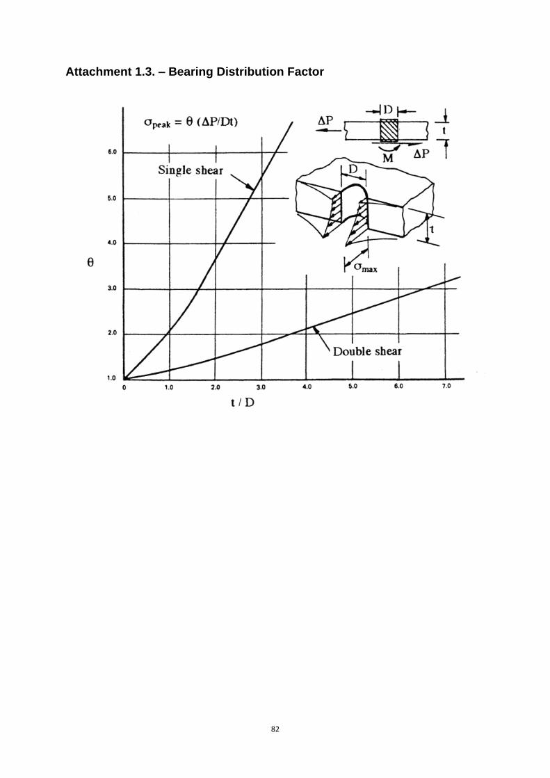
82
Attachment 1.3. – Bearing Distribution Factor
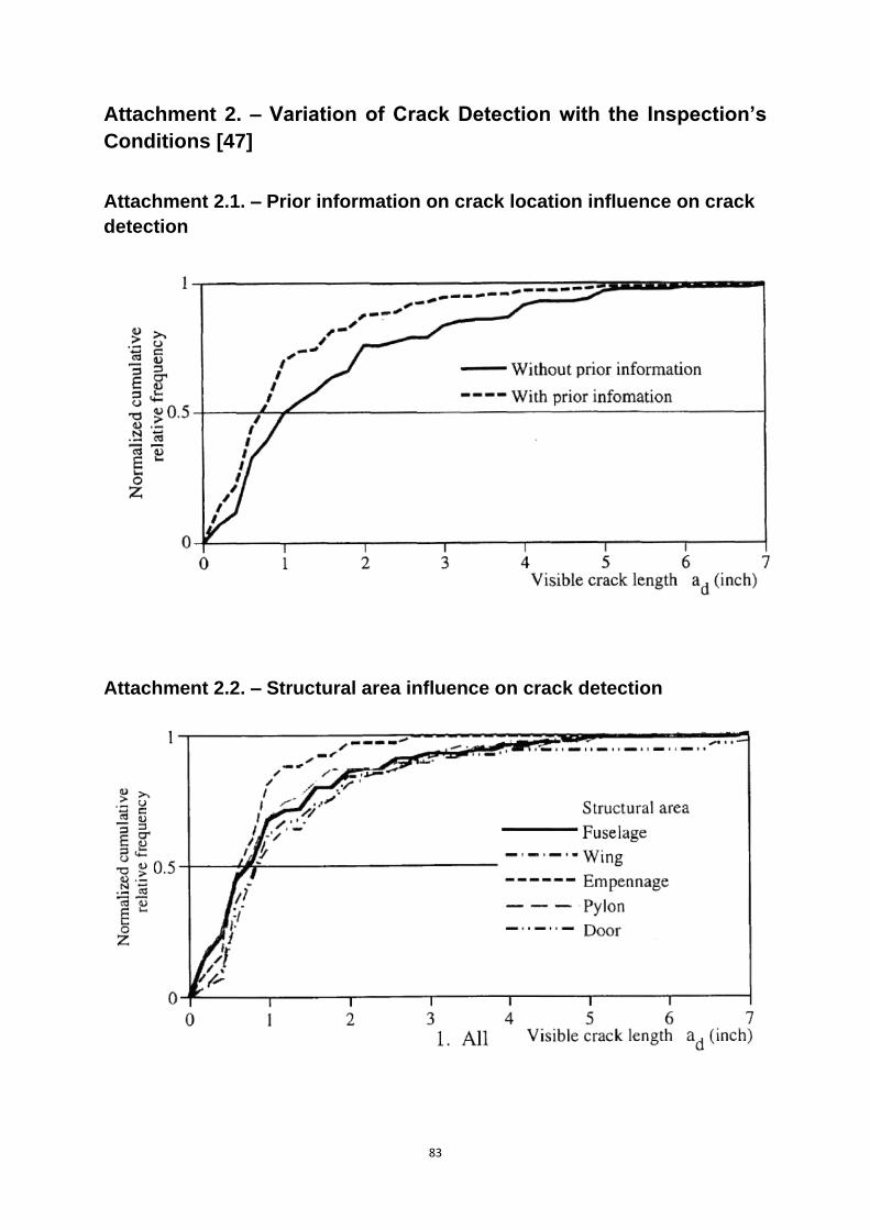
83
Attachment 2. – Variation of Crack Detection with the Inspection’s
Conditions [47]
Attachment 2.1. – Prior information on crack location influence on crack
detection
Attachment 2.2. – Structural area influence on crack detection
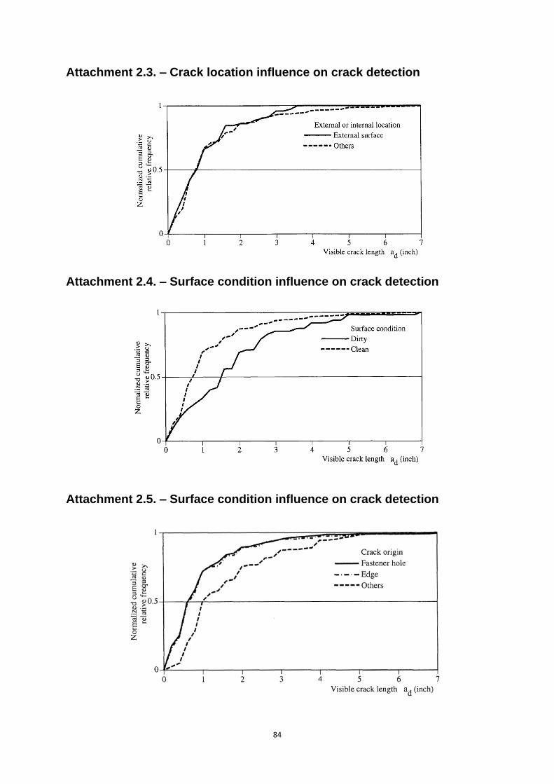
84
Attachment 2.3. – Crack location influence on crack detection
Attachment 2.4. – Surface condition influence on crack detection
Attachment 2.5. – Surface condition influence on crack detection
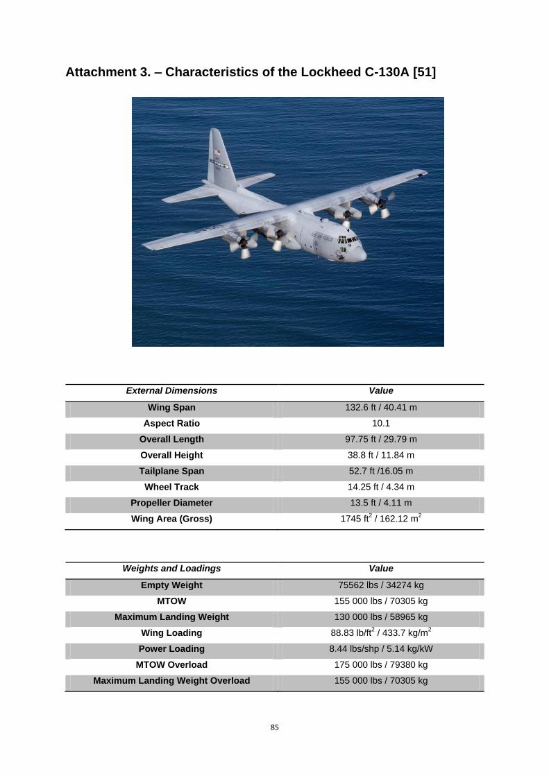
85
Attachment 3. – Characteristics of the Lockheed C-130A [51]
External Dimensions Value
Wing Span 132.6 ft / 40.41 m
Aspect Ratio 10.1
Overall Length 97.75 ft / 29.79 m
Overall Height 38.8 ft / 11.84 m
Tailplane Span 52.7 ft /16.05 m
Wheel Track 14.25 ft / 4.34 m
Propeller Diameter 13.5 ft / 4.11 m
Wing Area (Gross) 1745 ft2 / 162.12 m
2
Weights and Loadings Value
Empty Weight 75562 lbs / 34274 kg
MTOW 155 000 lbs / 70305 kg
Maximum Landing Weight 130 000 lbs / 58965 kg
Wing Loading 88.83 lb/ft2 / 433.7 kg/m
2
Power Loading 8.44 lbs/shp / 5.14 kg/kW
MTOW Overload 175 000 lbs / 79380 kg
Maximum Landing Weight Overload 155 000 lbs / 70305 kg