University of Central Florida University of Central Florida

STARS STARS

Electronic Theses and Dissertations, 2004-2019

2004

Performance Of Interface Elements In The Finite Element Method Performance Of Interface Elements In The Finite Element Method

Kairas Rabadi University of Central Florida

Part of the Mechanical Engineering Commons

Find similar works at: https://stars.library.ucf.edu/etd

University of Central Florida Libraries http://library.ucf.edu

This Masters Thesis (Open Access) is brought to you for free and open access by STARS. It has been accepted for

inclusion in Electronic Theses and Dissertations, 2004-2019 by an authorized administrator of STARS. For more

information, please contact STARS@ucf.edu.

STARS Citation STARS Citation Rabadi, Kairas, "Performance Of Interface Elements In The Finite Element Method" (2004). Electronic Theses and Dissertations, 2004-2019. 226. https://stars.library.ucf.edu/etd/226

PERFORMANCE OF INTERFACE ELEMENTS IN THE FINITE ELEMENT METHOD

by

KAIRAS S. RABADI B.E. N.E.D. University of Engineering & Technology, Karachi, 2001

A thesis submitted in partial fulfillment of the requirements for the degree of Master of Science

from the Department of Mechanical, Materials and Aerospace Engineering in the College of Engineering and Computer Science

at the University of Central Florida Orlando, Florida

Fall Term 2004

© 2004 Kairas S. Rabadi

ii

ABSTRACT

The objective of this research is to assess the performance of interface elements in the

finite element method. Interface elements are implemented in the finite element codes such as

MSC.NASTRAN, which is used in this study. Interface elements in MSC.NASTRAN provide a

tool to transition between a shell-meshed region to another shell-meshed region as well as from a

shell-meshed region to a solid-meshed region. Often, in practice shell elements are layered on

shell elements or on solid elements without the use of interface elements. This is potentially

inaccurate arising in mismatched degrees of freedom. In the case of a shell-to-shell interface, we

consider the case in which the two regions have mismatched nodes along the boundary. Interface

elements are used to connect these mismatched nodes. The interface elements are especially

useful in global/local analysis, where a region with a dense mesh interfaces to a region with a

less dense mesh. Interface elements are used to help avoid using special transition elements

between two meshed regions. This is desirable since the transition elements can be severely

distorted and cause poor results. Accurate results are obtained in shell-shell and shell-solid

combinations. The most interesting result is that not using interface elements can lead to severe

inaccuracies. This difficulty is illustrated by computing the stress concentration of a sharp

elliptical hole.

iii

ACKNOWLEDGEMENTS

I would like to take this opportunity to express my sincere appreciation to my professor

and advisor, Dr. David Nicholson, who has helped and guided me throughout the course of this

research.

I would like to thank Dr. Richard Zarda, who suggested this research topic, and has

helped me at every step of this research.

I would also like to thank my committee members; Dr. Alain Kassab and Dr. Quan Wang

for being on my thesis defense committee, and my colleague Eric Teuma for his constant support

and encouragement.

Last but not the least, I would like to thank my parents, my family, and the Dashtaki

family, for their enduring support in my academic pursuit.

iv

TABLE OF CONTENTS

LIST OF TABLES......................................................................................................................... vi LIST OF FIGURES ...................................................................................................................... vii CHAPTER 1 INTRODUCTION .................................................................................................... 1 CHAPTER 2 LITERATURE REVIEW ......................................................................................... 4 CHAPTER 3 MATHEMATICAL FORMULATION OF INTERFACE ELEMENTS................. 5 CHAPTER 4 SHELL-TO-SHELL INTERFACE ELEMENT....................................................... 8

4.1 Introduction........................................................................................................................... 8 4.2 Quarter-Plate Model............................................................................................................ 10

4.2.1 Mesh of the Quarter-Plate with Element Ratio 1:1...................................................... 11 4.2.2 Mesh of the Quarter Plate with unequal Elements....................................................... 18 4.2.3 Mesh of the Quarter Plate Model using Transition Elements...................................... 21

4.3 Conclusion .......................................................................................................................... 27 CHAPTER 5 shell-to-solid interface elements ............................................................................. 28

5.1 Introduction......................................................................................................................... 28 5.2 Cantilever Beam Model ...................................................................................................... 29 5.3 Quarter Plate Model............................................................................................................ 33

5.3.1Quarter Plate Model - Case 1........................................................................................ 33 5.3.2 Quarter Plate Model - Case 2....................................................................................... 42 5.3.3 Quarter Plate Model - Case 3....................................................................................... 49 5.3.4 Transition Elements ..................................................................................................... 56 5.3.5 Conclusion ................................................................................................................... 63

5.4 Non-linear Model................................................................................................................ 64 CHAPTER 6 DISCUSSION......................................................................................................... 74

6.1 For the shell-to-shell interface element – GMINTC........................................................... 75 6.2 For the shell-to-solid interface element – RSSCON........................................................... 76

CHAPTER 7 CONCLUSION....................................................................................................... 77 REFERENCES ............................................................................................................................. 78

v

LIST OF TABLES

Table 4-1: Summary of Results obtained for the GMINTC element............................................ 27 Table 4-2: Summary of Results obtained for the GMINTC element with Transition Elements .. 27Table 5-1: Summary of Results for the Cantilever Beam Model ................................................. 32 Table 5-2: Summary of Results obtained with the RSSCON element ......................................... 62 Table 5-3: Summary of Results obtained with the RSSCON element in the case of transition

elements ................................................................................................................................ 62 Table 5-4: Summary of Results obtained with the RSSCON element ......................................... 63 Table 5-5: Summary of Results obtained with the RSSCON element in the case of transition

elements ................................................................................................................................ 63

vi

LIST OF FIGURES

Figure 1-1: Distinct models on different workstations ................................................................... 2 Figure 4-1: Two regions of unequal shell mesh densities............................................................... 8 Figure 4-2: Three noded transition shell mesh ............................................................................... 9 Figure 4-3: Illustrating the use of Interface elements ..................................................................... 9 Figure 4-4: Quarter Plate model with dimensions ........................................................................ 10 Figure 4-5: Two shell meshed regions.......................................................................................... 11 Figure 4-6: Two shell meshed regions with unmatched nodes..................................................... 12 Figure 4-7: An enlarged view of the mismatched nodes on the top edge..................................... 13 Figure 4-8: An enlarged view of the mismatched nodes on the right edge .................................. 13 Figure 4-9: Input Panel in I-DEAS9 for Force ............................................................................. 14 Figure 4-10: Input Panel for Constraints on left edge................................................................... 14 Figure 4-11: Input Panel for constraints on bottom edge ............................................................. 15 Figure 4-12: Plot for stresses in the y-direction............................................................................ 17 Figure 4-13: Mesh of the quarter plate with one region denser than the other............................. 18 Figure 4-14: A closer look at the denser mesh and the boundary of mismatched nodes.............. 19 Figure 4-15: An enlarged view of the top edge of the boundary of the mismatched nodes ......... 19 Figure 4-16: Plot of the Stress in the y-direction.......................................................................... 20 Figure 4-17: Mesh of one region of the quarter plate ................................................................... 21 Figure 4-18: Mesh of second region of the quarter plate.............................................................. 22 Figure 4-19: Mesh of the two regions of the quarter plate ........................................................... 22 Figure 4-20: Mesh of the two regions brought together ............................................................... 23 Figure 4-21: An enlarged view of the mismatched nodes along the boundary of the two regions

............................................................................................................................................... 24Figure 4-22: An enlarged view of the transition elements with coincident nodes........................ 24 Figure 4-23: Plot of the stress in the y-direction using interface elements................................... 25 Figure 4-24: Plot of the stress in the y-direction without interface elements ............................... 26 Figure 5-1: Illustrating the position of shell and solid nodes........................................................ 28 Figure 5-2: Cantilever beam model .............................................................................................. 29 Figure 5-3: Displacement Plot in I-DEAS9.................................................................................. 30 Figure 5-4: Non-layered Stress plot in MSC.NASTRAN ............................................................ 31 Figure 5-5: Stress plot in MSC.NASTRAN ................................................................................. 31 Figure 5-6: Isometric view of the quarter plate showing the two regions; surface and volume... 34 Figure 5-7: Showing the front and isometric views of the meshed plate...................................... 35 Figure 5-8: Meshed plate with Boundary conditions applied....................................................... 35 Figure 5-9: Plot of the Stress in the y-direction............................................................................ 36 Figure 5-10: Plot of the stress in the x-direction........................................................................... 37 Figure 5-11: View of the mesh without interface elements.......................................................... 38

vii

Figure 5-12: Stress Plot in the y-direction without Interface Elements........................................ 39 Figure 5-13: Enlarged view of the area of concern....................................................................... 40 Figure 5-14: Stress Plot; Without Interface element (left) and with interface elements (right) ... 40 Figure 5-15: Plot of the stress in the x-direction........................................................................... 41 Figure 5-16: Quarter Plate Model for Case 2................................................................................ 42 Figure 5-17: Quarter Plate Model mesh with Boundary Conditions ............................................ 43 Figure 5-18: Stress Plot in the y-direction .................................................................................... 44 Figure 5-19: Plot of the stresses in the x-direction ....................................................................... 45 Figure 5-20: Stress Plot in the y direction without interface elements ......................................... 46 Figure 5-21: Enlarged view of the area of concern....................................................................... 46 Figure 5-22: Stress Plot; Without Interface element (left) and with interface elements (right) ... 47 Figure 5-23: Plot of stresses in the x-direction ............................................................................. 48 Figure 5-24: Quarter Plate model for Case 3 ............................................................................... 49 Figure 5-25: Mesh of Quarter Plate Model Case 3 with Boundary Conditions............................ 50 Figure 5-26: Stress plot in the y-direction .................................................................................... 51 Figure 5-27: Stress plot in the x-direction .................................................................................... 52 Figure 5-28: Stress Plot in the y direction without interface elements ......................................... 53 Figure 5-29: Enlarged view of the area of concern....................................................................... 54 Figure 5-30: Stress Plot; Without Interface element (left) and with interface elements (right) ... 54 Figure 5-31: Plot of the stresses in the x-direction ....................................................................... 55 Figure 5-32: Shell and Solid mesh along with transition shell elements...................................... 56 Figure 5-33: Transition Elements stepping down from three shell elements to one shell element

............................................................................................................................................... 57Figure 5-34: Transition Elements stepping down from three shell elements to one shell element

in the case of interface elements ........................................................................................... 57 Figure 5-35: Stress plot in the y-direction without Interface Elements ........................................ 58 Figure 5-36: Stress plot in the x-direction without Interface Elements ........................................ 59 Figure 5-37: Stress plot in the y-direction in the case of Interface Elements ............................... 60 Figure 5-38: Stress plot in the x-direction in the case of Interface Elements ............................... 61 Figure 5-39: Solid Model used for Non-Linear Analysis ............................................................. 64 Figure 5-40: Mesh of the symmetric solid model ......................................................................... 65 Figure 5-41: Hyperelastic Material card used in MSC.NASTRAN ............................................. 66 Figure 5-42: Front view of the Cylindrical Model........................................................................ 67 Figure 5-43: Showing the three surfaces for boundary condition application.............................. 67 Figure 5-44: Isometric View of the Mesh and Boundary Conditions........................................... 69 Figure 5-45: Side view of the mesh and Force ............................................................................. 69 Figure 5-46: Plot for Maximum Displacement With Interface elements ..................................... 71 Figure 5-47: X-Y graph plot for Load vs. Displacement for Node # 81 ...................................... 72 Figure 5-48: Plot for Maximum Displacement Without Interface elements ................................ 73

viii

CHAPTER 1 INTRODUCTION

When performing global/local analysis, the issue of connecting dissimilar meshes

often arises, especially when refinement is performed. One method of connecting these

dissimilar meshes is to use interface elements, which have been developed by the NASA

Langley Research Center. In MSC.NASTRAN 2001 and thereafter these interface

elements have been implemented.

The problem of connecting dissimilar meshes at a common interface is a major

one in finite element analysis. Such interfaces can result from a variety of sources, which

can be divided into two categories: generated by the analyst, and generated by the

analysis program.

Dissimilar meshes generated by the analyst can occur with global/local analysis,

where part of the structure is modeled as the area of primary interest, in which detailed

stress distributions are required, and part of the structure is modeled as the area of

secondary interest. Generally the area of primary interest has a finer mesh than the area of

secondary interest, and therefore a transition area is required. Severe transitions generally

produce elements that are heavily distorted, which can result in poor stresses and poor

load transfers into the area of primary interest.

To illustrate the use of interface elements, an example of an airplane model is

given below. Development of an airframe finite element model requires division of

engineering labor. Models are often built by two or more companies remotely located,

1

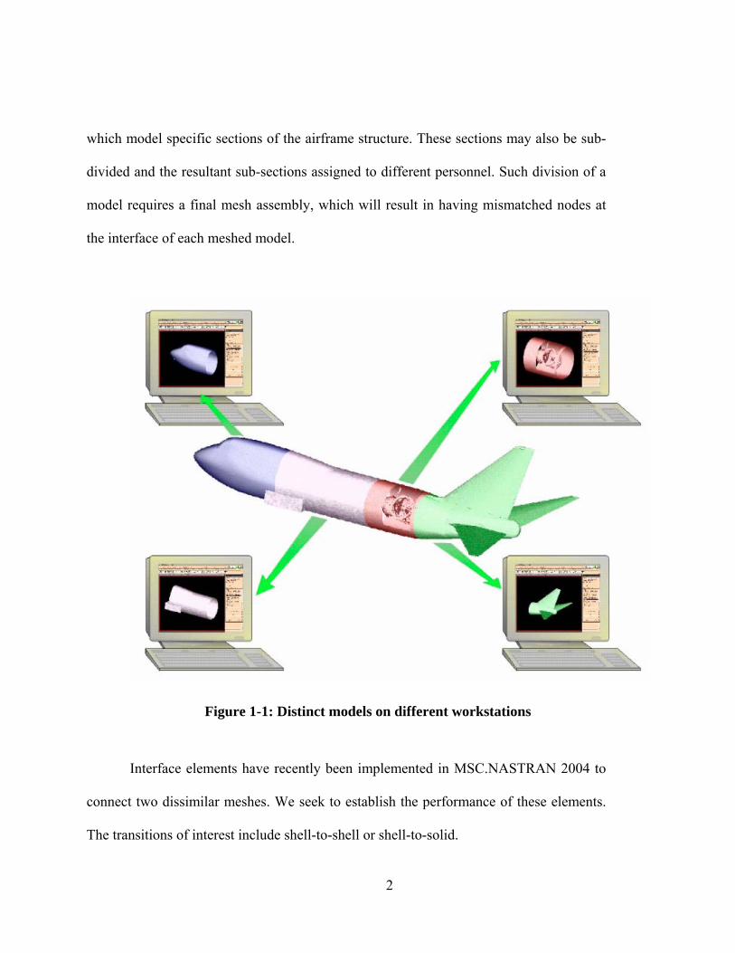
which model specific sections of the airframe structure. These sections may also be sub-

divided and the resultant sub-sections assigned to different personnel. Such division of a

model requires a final mesh assembly, which will result in having mismatched nodes at

the interface of each meshed model.

Figure 1-1: Distinct models on different workstations

Interface elements have recently been implemented in MSC.NASTRAN 2004 to

connect two dissimilar meshes. We seek to establish the performance of these elements.

The transitions of interest include shell-to-shell or shell-to-solid.

2

As previously stated, the goal is to evaluate the performance of the interface

elements implemented in MSC.NASTRAN 2004. I-DEAS9 in used for the initial model

development and I-DEAS9 and PATRAN is used to portray the output graphically.

The major conclusions are as follows:

• Interface elements provided accurate results in the case of a sharp

elliptical crack. However, not using interface elements as is common

practice gave very inaccurate results. Good practice calls for using

interface elements.

• The shell-shell and shell-solid cases gave accurate results using interface

elements, provided there is no discontinuity in nodal density.

• If there is a discontinuity in nodal density, very inaccurate results were

obtained despite using Interface elements.

• Accurate results were obtained in a nonlinear problem using interface

elements.

3

CHAPTER 2 LITERATURE REVIEW

Since the introduction of the finite element method there has been the need to connect

mismatched nodes along the boundary of the element interface. Previously the issue was

addressed by moving the nodes or writing multi-point constraint equations on the interfaces.

Moving the nodes is very cumbersome and may heavily distort the element. The biggest

restriction of moving the nodes is that both sides of the interface must have the same number and

type of elements. The other approach of writing multi-point constraint equations has its

disadvantages as well. Multi-point constraints equations are used for a node between two nodes,

where the node in the center is allowed to slide between these two nodes. However, multi-point

constraint equations provide additional relationships for the existing degrees of freedom on the

interface, and in the process may result in additional local stiffness.

The new method of connecting mismatched nodes using Interface Elements developed by

NASA Langley Research Center has been implemented in MSC.NASTRAN.

4

CHAPTER 3 MATHEMATICAL FORMULATION OF INTERFACE

ELEMENTS

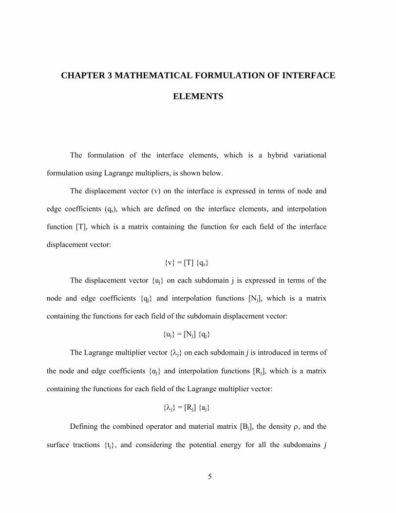
The formulation of the interface elements, which is a hybrid variational

formulation using Lagrange multipliers, is shown below.

The displacement vector (v) on the interface is expressed in terms of node and

edge coefficients (qs), which are defined on the interface elements, and interpolation

function [T], which is a matrix containing the function for each field of the interface

displacement vector:

v = [T] qs

The displacement vector uj on each subdomain j is expressed in terms of the

node and edge coefficients qj and interpolation functions [Nj], which is a matrix

containing the functions for each field of the subdomain displacement vector:

uj = [Nj] qj

The Lagrange multiplier vector λj on each subdomain j is introduced in terms of

the node and edge coefficients αj and interpolation functions [Rj], which is a matrix

containing the functions for each field of the Lagrange multiplier vector:

λj = [Rj] aj

Defining the combined operator and material matrix [Bj], the density ρ, and the

surface tractions tj, and considering the potential energy for all the subdomains j

5

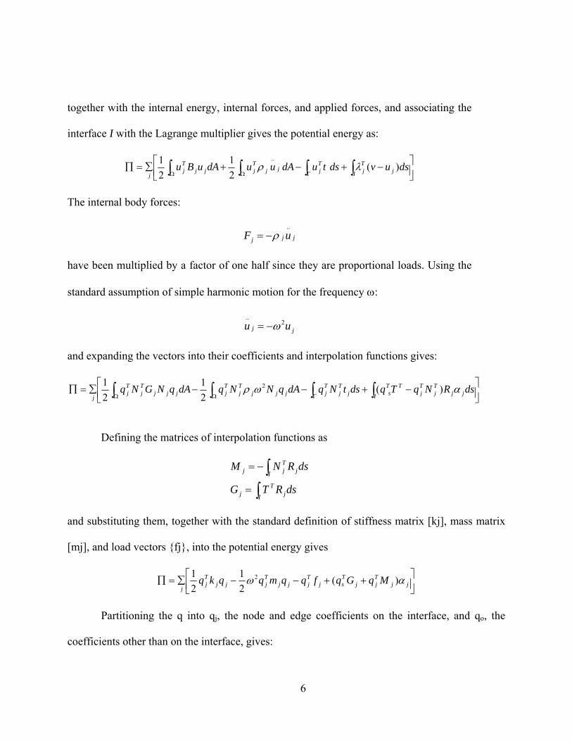
together with the internal energy, internal forces, and applied forces, and associating the

interface I with the Lagrange multiplier gives the potential energy as:

⎥⎦⎤

⎢⎣⎡ −+−+∑=∏ ∫ ∫ ∫∫ Ω ΓΩ I j

Tj

Tjjj

Tjjj

Tj

jdsuvdstudAuudAuBu )(

21

21 ..

λρ

The internal body forces:

jjj uF..

ρ−=

have been multiplied by a factor of one half since they are proportional loads. Using the

standard assumption of simple harmonic motion for the frequency ω:

jj uu 2..

ω−=

and expanding the vectors into their coefficients and interpolation functions gives:

⎥⎦⎤

⎢⎣⎡ −+−−∑=∏ ∫ ∫ ∫∫ Ω ΓΩ I jj

Tj

Tj

TTsj

Tj

Tjjjj

Tj

Tjjjj

Tj

Tj

jdsRNqTqdstNqdAqNNqdAqNGNq αωρ )(

21

21 2

Defining the matrices of interpolation functions as

∫∫

=

−=

I jT

j

I jTjj

dsRTG

dsRNM

and substituting them, together with the standard definition of stiffness matrix [kj], mass matrix

[mj], and load vectors fj, into the potential energy gives

⎥⎦⎤

⎢⎣⎡ ++−−∑=∏ jj

Tjj

Tsj

Tjjj

Tjjj

Tj

jMqGqfqqmqqkq αω )(

21

21 2

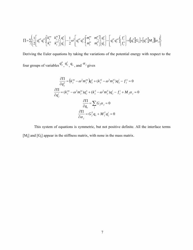
Partitioning the q into qj, the node and edge coefficients on the interface, and qo, the

coefficients other than on the interface, gives:

6

] ] ] [ ][ ] [ ][ ]( ) ⎪⎭

⎪⎬⎫

⎪⎩

⎪⎨⎧

⎢⎢⎣

⎡++

⎭⎬⎫

⎩⎨⎧

−⎢⎢⎣

⎡

⎭⎬⎫

⎩⎨⎧⎥⎦

⎤⎢⎣

⎡−

⎭⎬⎫

⎩⎨⎧

⎢⎢⎣

⎡⎥⎦

⎤⎢⎣

⎡∑=∏ jj

iTjj

Tso

j

ijoT

jiTji

j

oj

iij

ioj

oij

oojiT

joTji

j

oj

iij

ioj

ij

oojiT

joTj

jMqGq

ff

qqqq

mmmm

qqqq

kkkk

qq αω20

21

21

Deriving the Euler equations by taking the variations of the potential energy with respect to the

four groups of variables , , , and ojq i

jq sq jα gives

( ) 0)( 22 =−−+−=∂Π∂ o

jij

oij

oij

oj

ooj

oojo

j

fqmkqmkq

ωω

0)()( 22 =+−−+−=∂Π∂

jjij

ij

iij

iij

oj

ioj

ooji

j

Mfqmkqmkq

αωω

∑ ==∂Π∂

jjj

s

Gq

0α

0=+=∂Π∂ i

jTjs

Tj

j

qMqGα

This system of equations is symmetric, but not positive definite. All the interface terms

[Mj] and [Gj] appear in the stiffness matrix, with none in the mass matrix.

7

CHAPTER 4 SHELL-TO-SHELL INTERFACE ELEMENT

4.1 Introduction

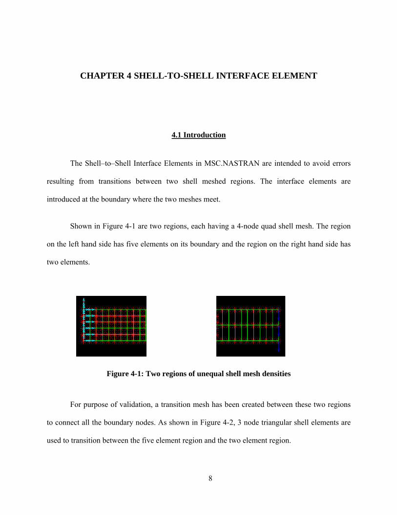
The Shell–to–Shell Interface Elements in MSC.NASTRAN are intended to avoid errors

resulting from transitions between two shell meshed regions. The interface elements are

introduced at the boundary where the two meshes meet.

Shown in Figure 4-1 are two regions, each having a 4-node quad shell mesh. The region

on the left hand side has five elements on its boundary and the region on the right hand side has

two elements.

Figure 4-1: Two regions of unequal shell mesh densities

For purpose of validation, a transition mesh has been created between these two regions

to connect all the boundary nodes. As shown in Figure 4-2, 3 node triangular shell elements are

used to transition between the five element region and the two element region.

8

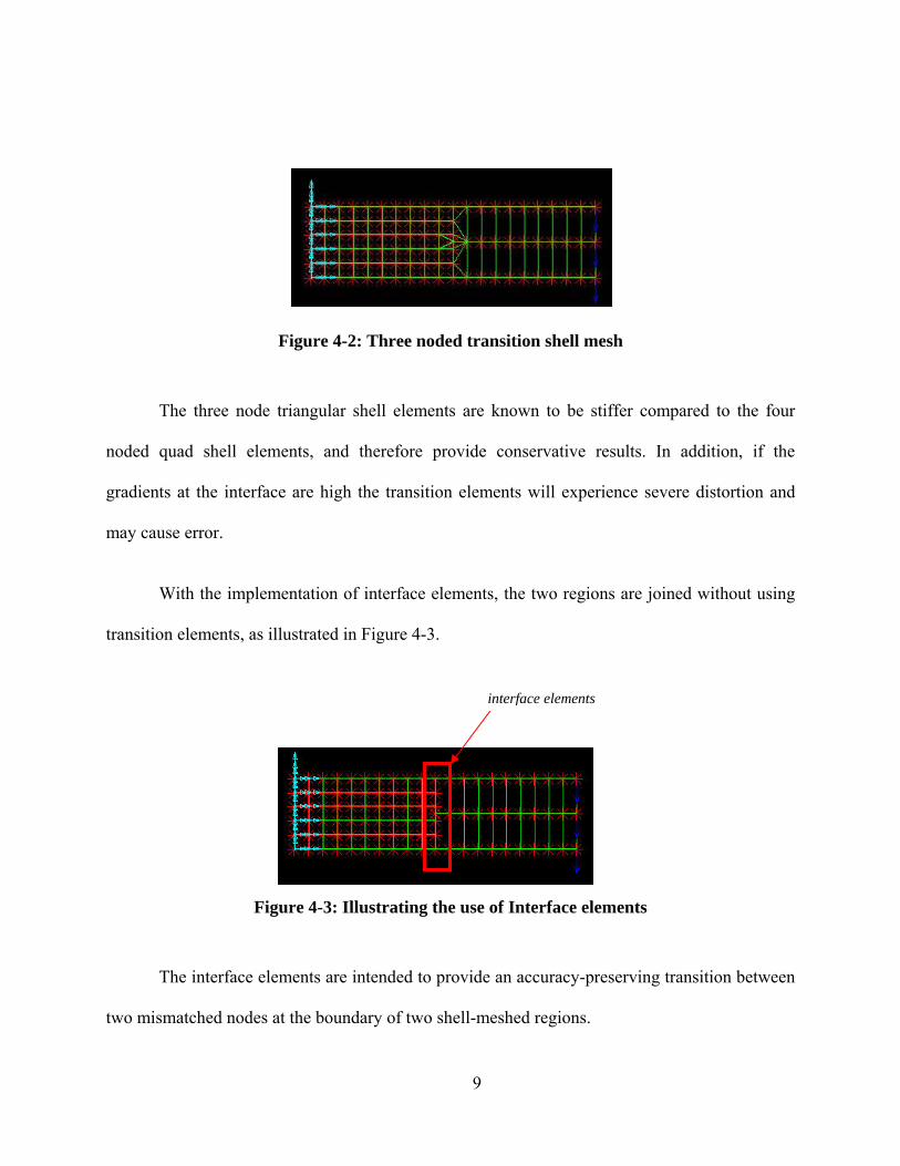
Figure 4-2: Three noded transition shell mesh

The three node triangular shell elements are known to be stiffer compared to the four

noded quad shell elements, and therefore provide conservative results. In addition, if the

gradients at the interface are high the transition elements will experience severe distortion and

may cause error.

With the implementation of interface elements, the two regions are joined without using

transition elements, as illustrated in Figure 4-3.

interface elements

Figure 4-3: Illustrating the use of Interface elements

The interface elements are intended to provide an accuracy-preserving transition between

two mismatched nodes at the boundary of two shell-meshed regions.

9

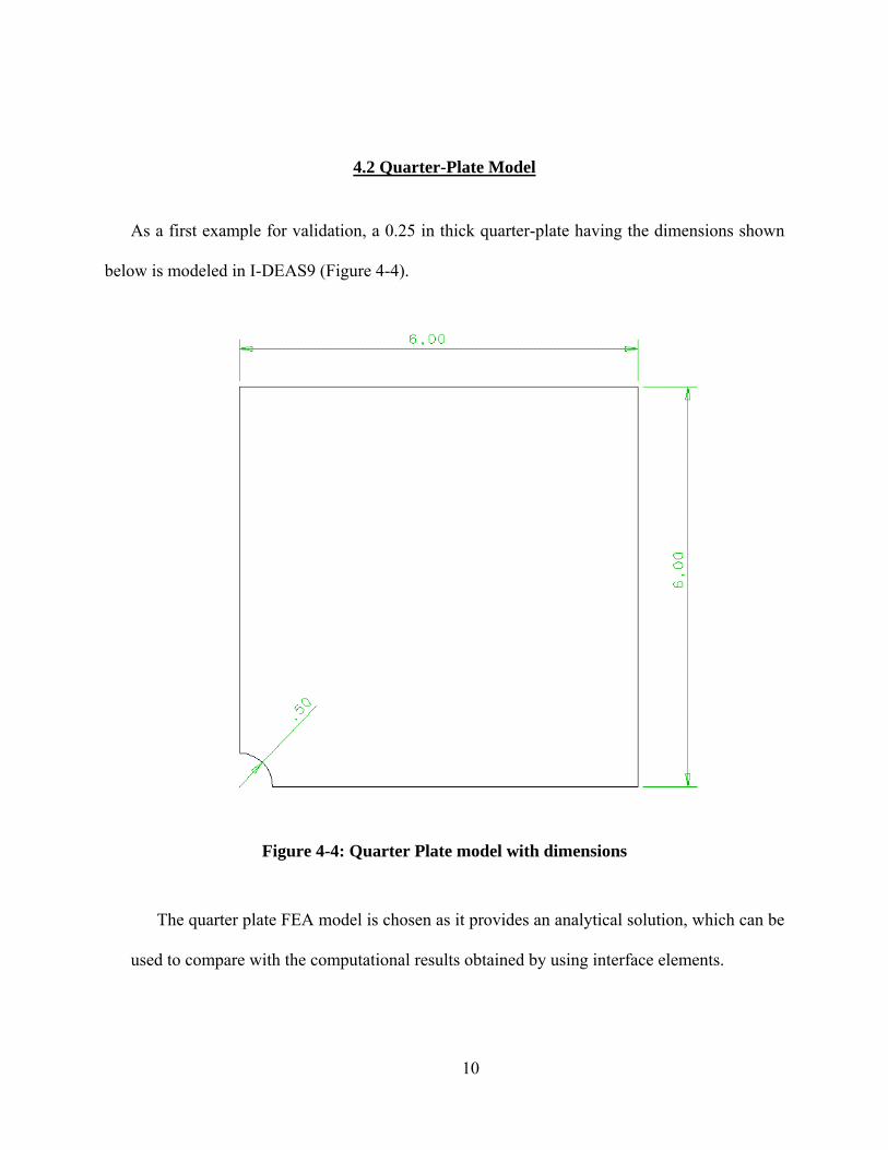
4.2 Quarter-Plate Model

As a first example for validation, a 0.25 in thick quarter-plate having the dimensions shown

below is modeled in I-DEAS9 (Figure 4-4).

Figure 4-4: Quarter Plate model with dimensions

The quarter plate FEA model is chosen as it provides an analytical solution, which can be

used to compare with the computational results obtained by using interface elements.

10

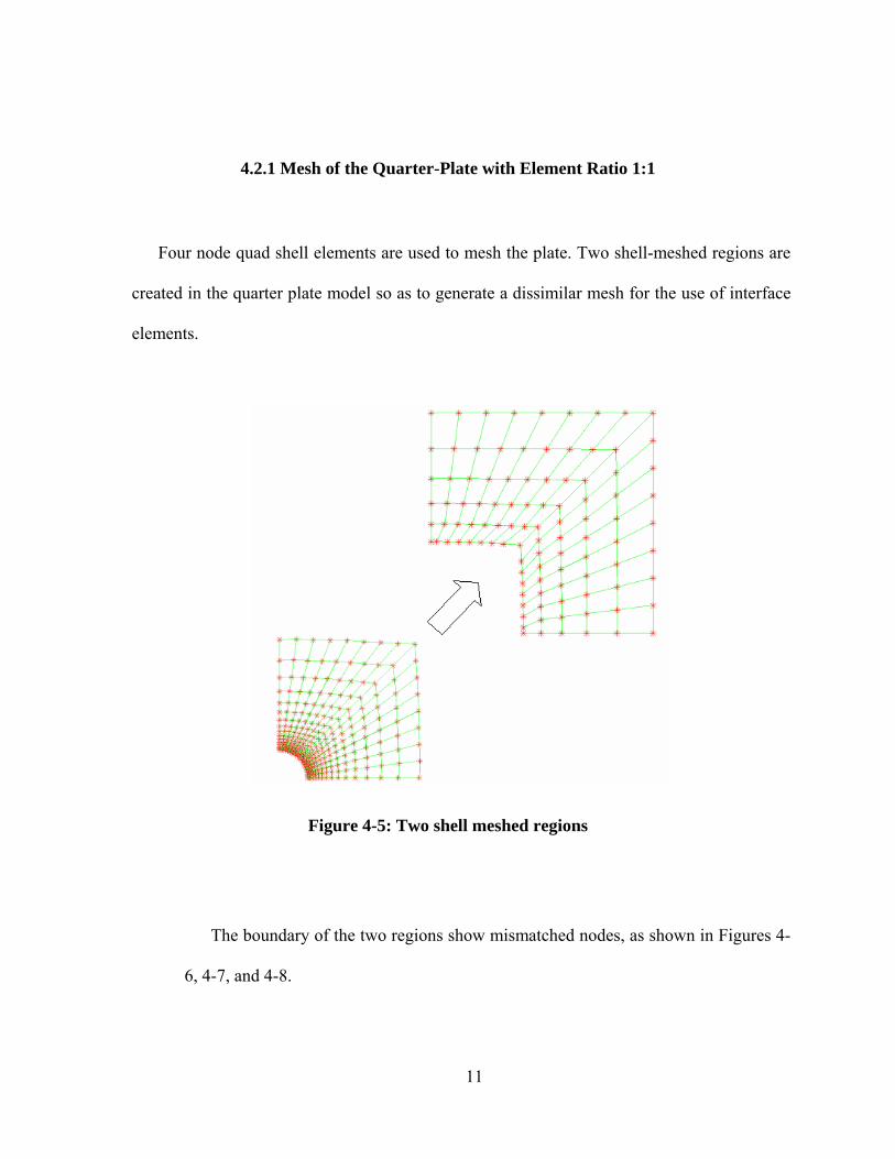
4.2.1 Mesh of the Quarter-Plate with Element Ratio 1:1

Four node quad shell elements are used to mesh the plate. Two shell-meshed regions are

created in the quarter plate model so as to generate a dissimilar mesh for the use of interface

elements.

Figure 4-5: Two shell meshed regions

The boundary of the two regions show mismatched nodes, as shown in Figures 4-

6, 4-7, and 4-8.

11

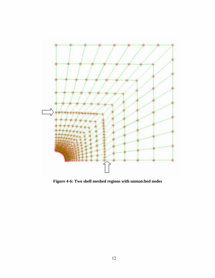
Figure 4-6: Two shell meshed regions with unmatched nodes

12

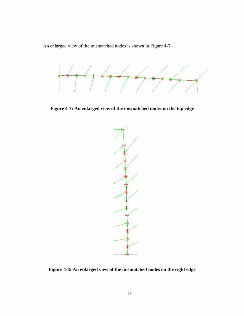
An enlarged view of the mismatched nodes is shown in Figure 4-7.

Figure 4-7: An enlarged view of the mismatched nodes on the top edge

Figure 4-8: An enlarged view of the mismatched nodes on the right edge

13

4.2.1.1 Boundary Conditions

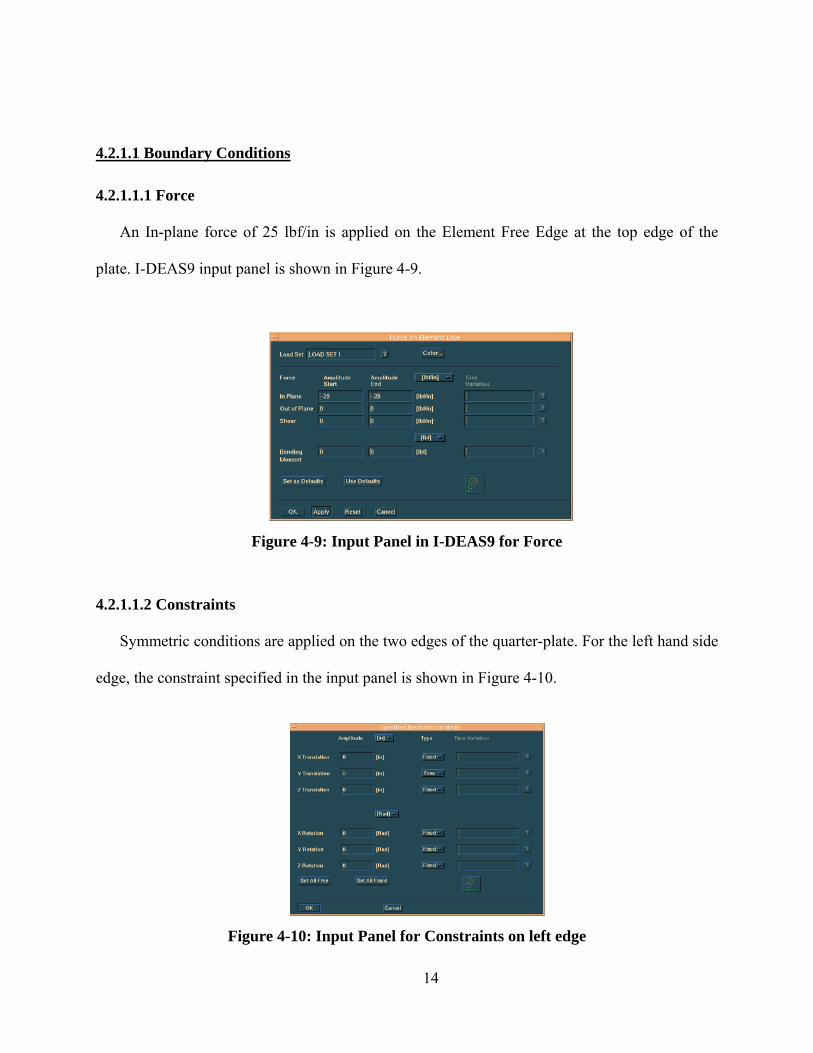
4.2.1.1.1 Force An In-plane force of 25 lbf/in is applied on the Element Free Edge at the top edge of the

plate. I-DEAS9 input panel is shown in Figure 4-9.

Figure 4-9: Input Panel in I-DEAS9 for Force

4.2.1.1.2 Constraints Symmetric conditions are applied on the two edges of the quarter-plate. For the left hand side

edge, the constraint specified in the input panel is shown in Figure 4-10.

Figure 4-10: Input Panel for Constraints on left edge

14

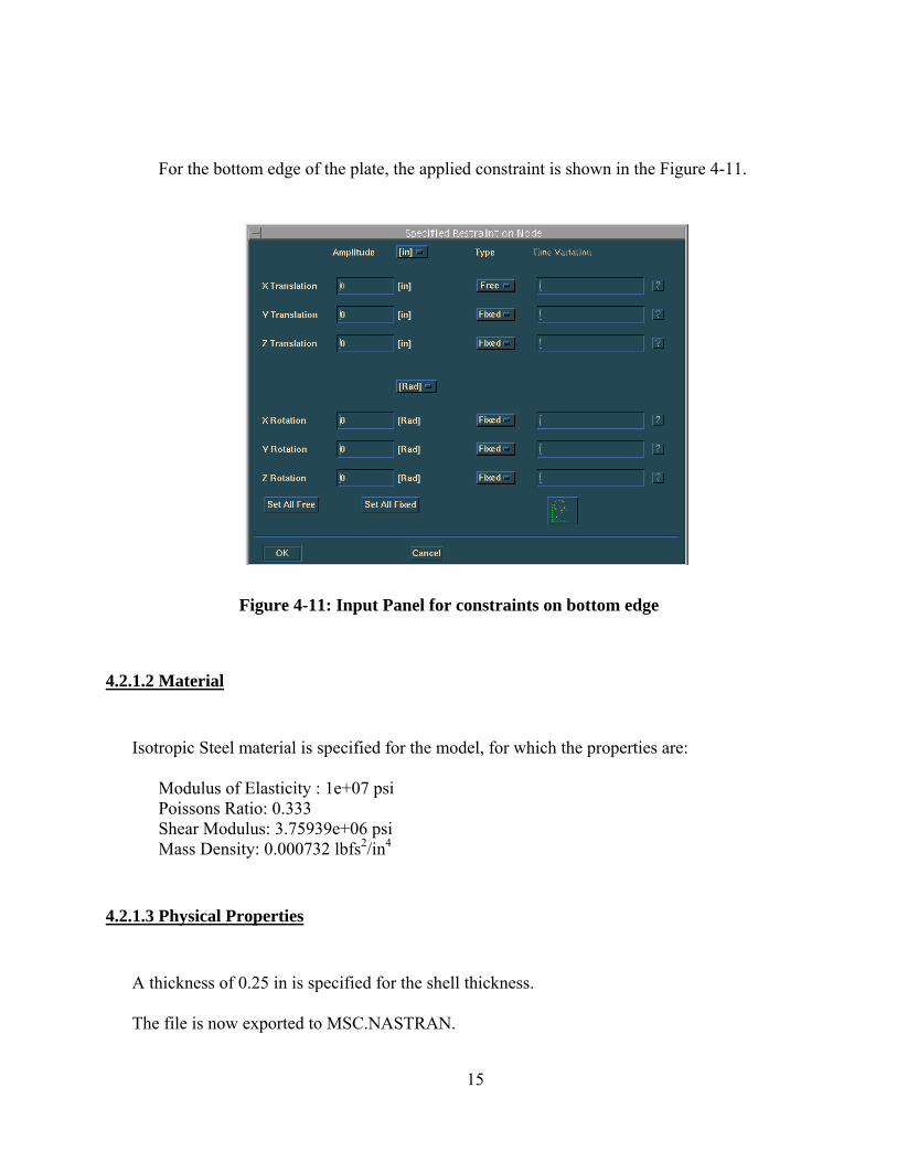
For the bottom edge of the plate, the applied constraint is shown in the Figure 4-11.

Figure 4-11: Input Panel for constraints on bottom edge

4.2.1.2 Material

Isotropic Steel material is specified for the model, for which the properties are:

Modulus of Elasticity : 1e+07 psi Poissons Ratio: 0.333 Shear Modulus: 3.75939e+06 psi Mass Density: 0.000732 lbfs2/in4

4.2.1.3 Physical Properties

A thickness of 0.25 in is specified for the shell thickness. The file is now exported to MSC.NASTRAN.

15

4.2.1.4 Introduction of Interface Elements in Bulk Data Entry in MSC.NASTRAN

After the I-DEAS9 model file is exported to NASTRAN it is necessary to modify the input

file within NASTRAN to exercise the interface elements. The following cards are introduced in

the Bulk Data Entry of MSC.NASTRAN.

GMBNDC GMINTC PINTC Two interface elements are used in this model because of the sharp 45° boundary at the

meeting of the two models.

4.2.1.5 Results

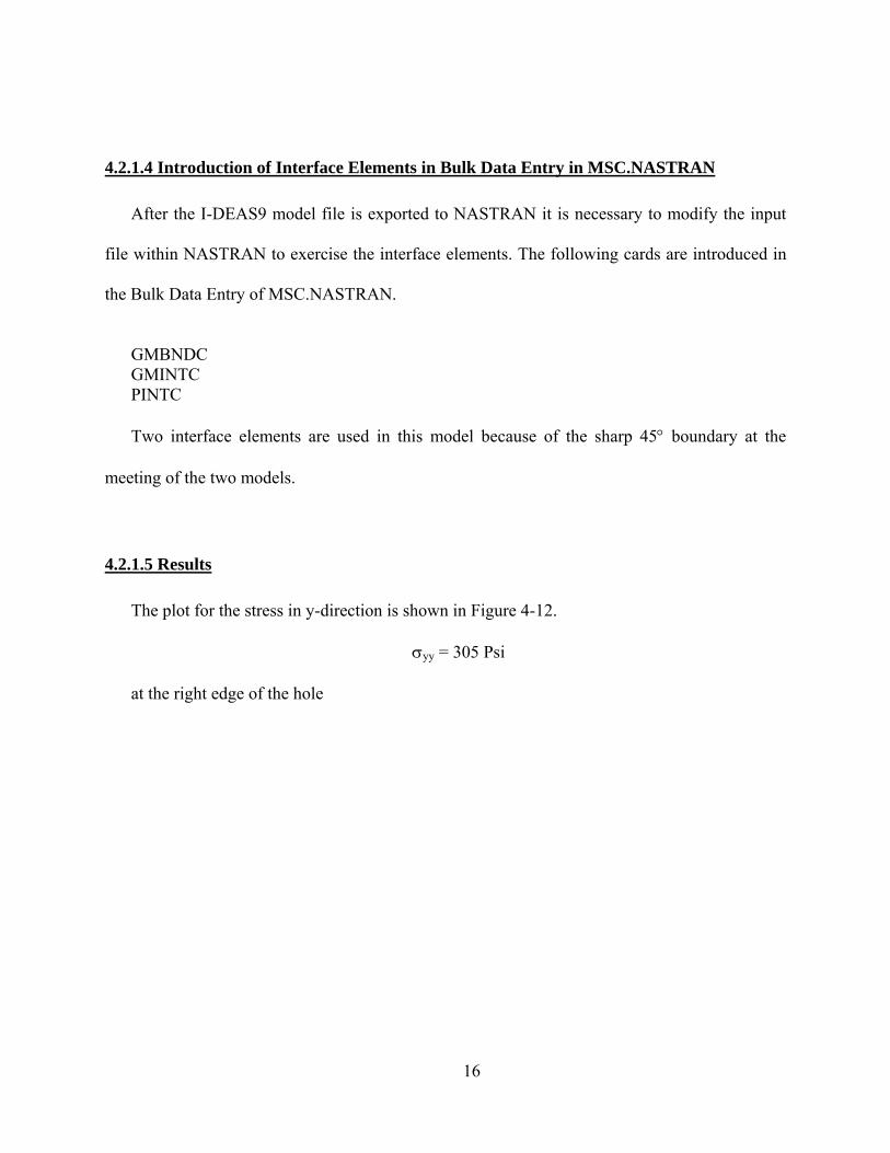
The plot for the stress in y-direction is shown in Figure 4-12.

σyy = 305 Psi

at the right edge of the hole

16

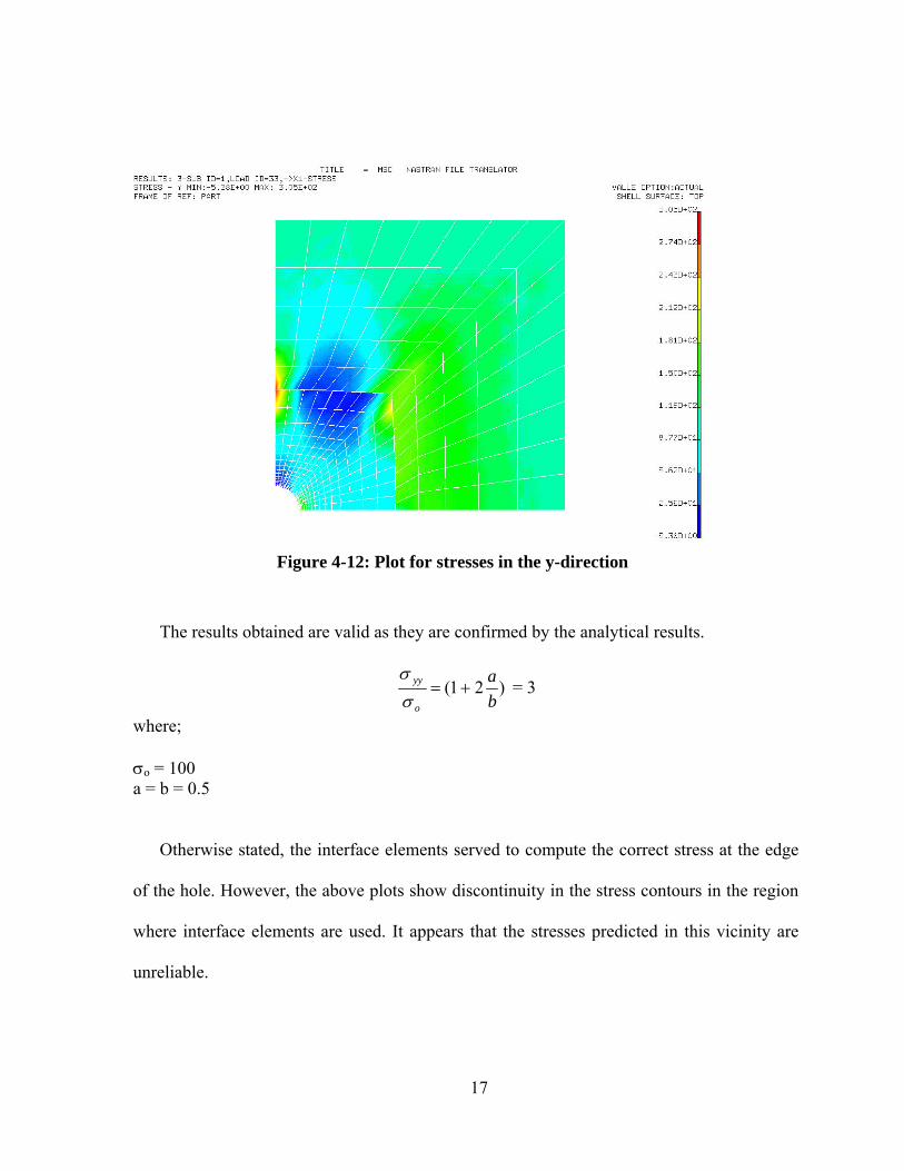
Figure 4-12: Plot for stresses in the y-direction

The results obtained are valid as they are confirmed by the analytical results.

)21(ba

o

yy +=σσ

= 3

where; σo = 100 a = b = 0.5

Otherwise stated, the interface elements served to compute the correct stress at the edge

of the hole. However, the above plots show discontinuity in the stress contours in the region

where interface elements are used. It appears that the stresses predicted in this vicinity are

unreliable.

17

4.2.2 Mesh of the Quarter Plate with unequal Elements

The above case is used again, this time, one the regions have a denser mesh as compared

to the other. There are 12 elements on the edge of the denser mesh to 8 elements on the

corresponding less dense mesh.

Figure 4-13: Mesh of the quarter plate with one region denser than the other

18

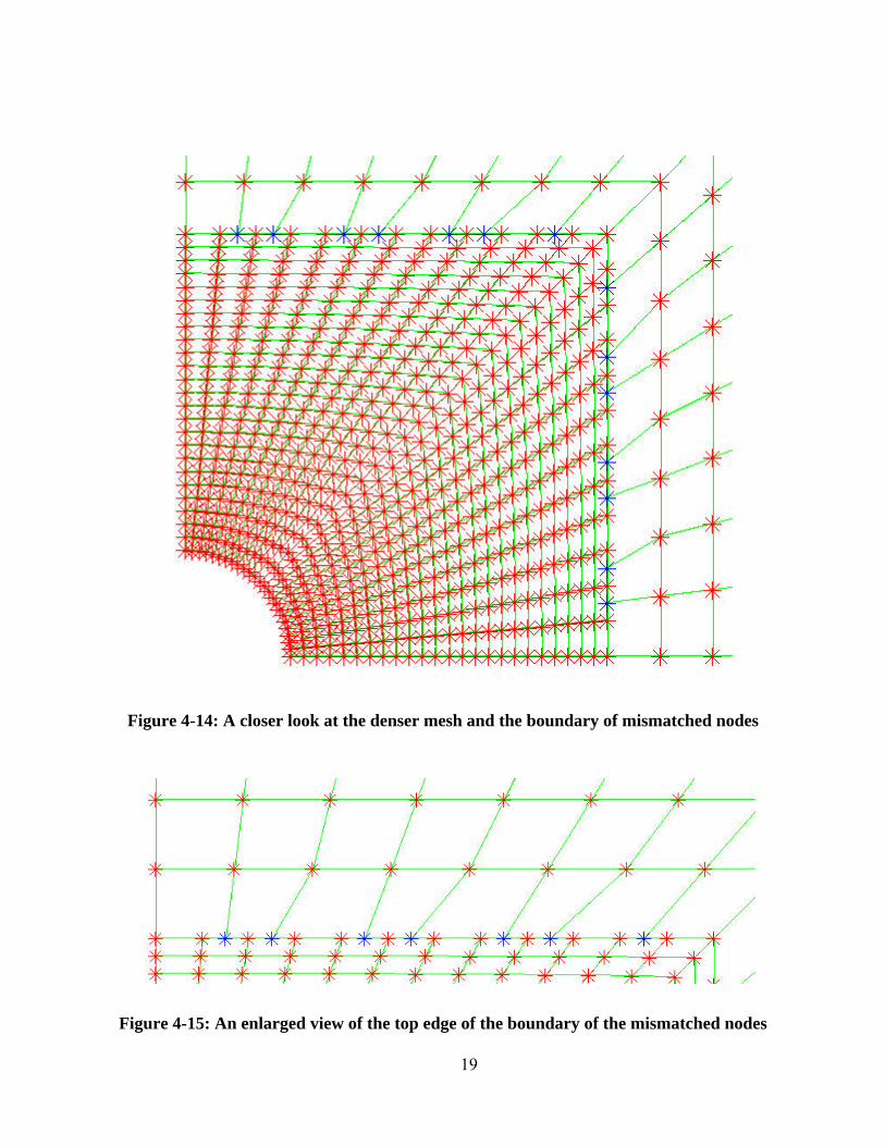
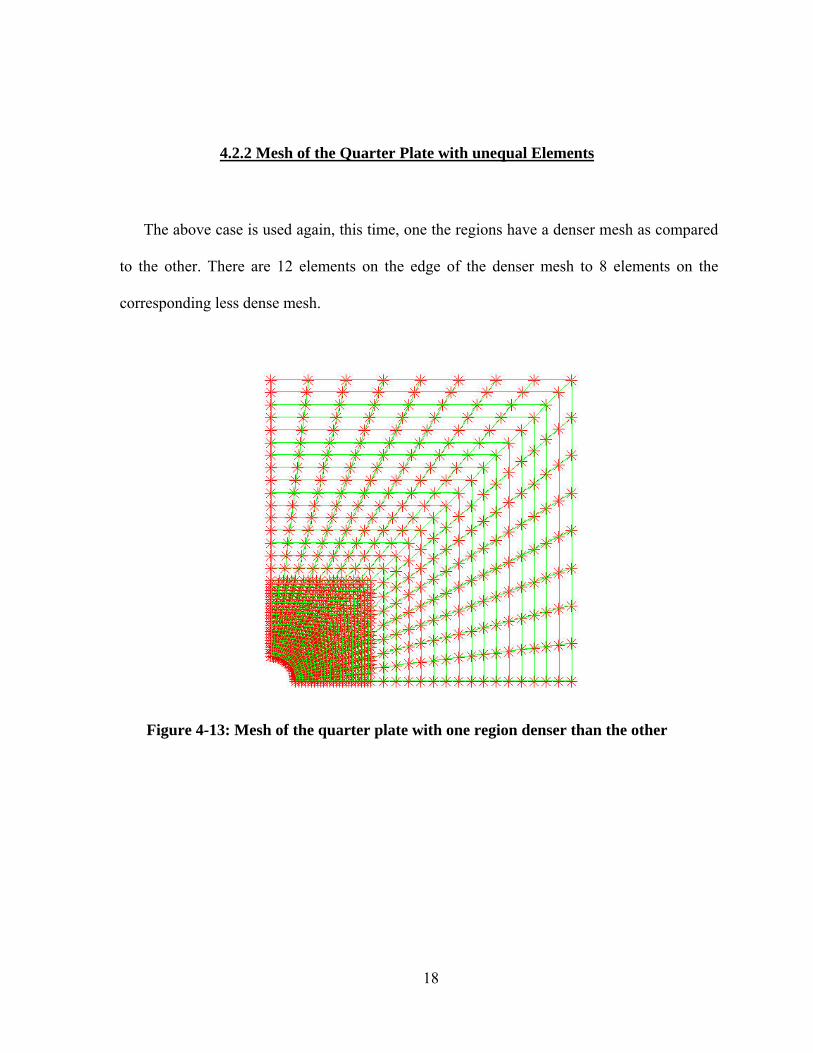
Figure 4-14: A closer look at the denser mesh and the boundary of mismatched nodes

Figure 4-15: An enlarged view of the top edge of the boundary of the mismatched nodes

19

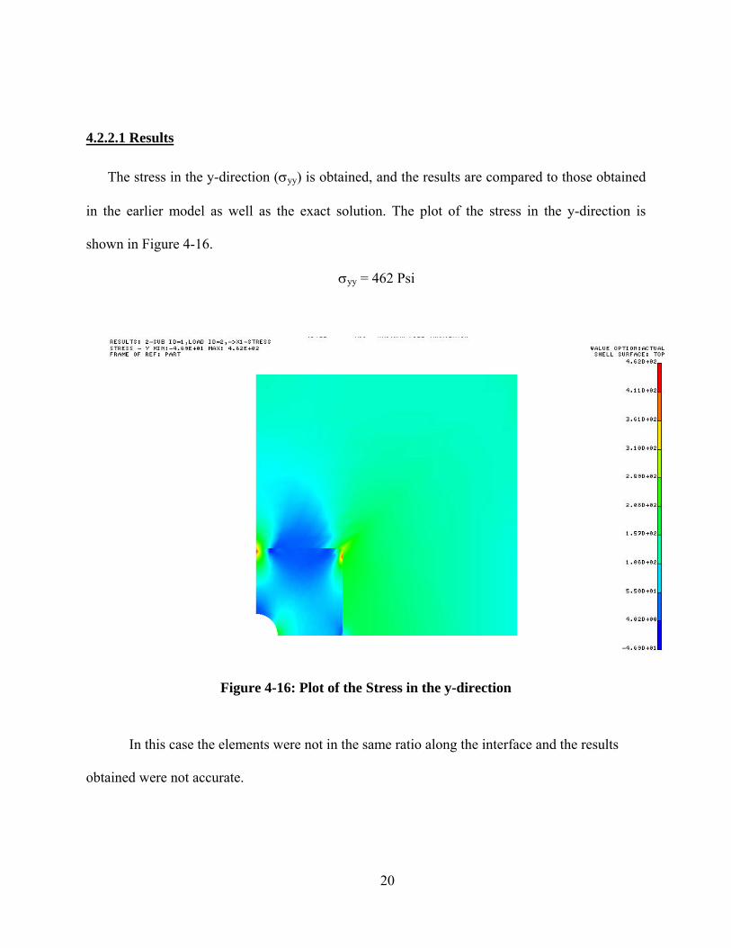
4.2.2.1 Results

The stress in the y-direction (σyy) is obtained, and the results are compared to those obtained

in the earlier model as well as the exact solution. The plot of the stress in the y-direction is

shown in Figure 4-16.

σyy = 462 Psi

Figure 4-16: Plot of the Stress in the y-direction

In this case the elements were not in the same ratio along the interface and the results

obtained were not accurate.

20

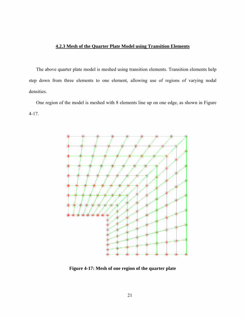
4.2.3 Mesh of the Quarter Plate Model using Transition Elements

The above quarter plate model is meshed using transition elements. Transition elements help

step down from three elements to one element, allowing use of regions of varying nodal

densities.

One region of the model is meshed with 8 elements line up on one edge, as shown in Figure

4-17.

Figure 4-17: Mesh of one region of the quarter plate

21

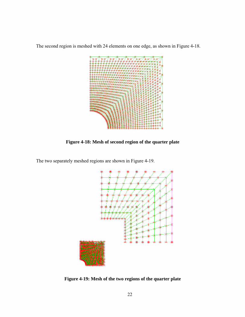
The second region is meshed with 24 elements on one edge, as shown in Figure 4-18.

Figure 4-18: Mesh of second region of the quarter plate

The two separately meshed regions are shown in Figure 4-19.

Figure 4-19: Mesh of the two regions of the quarter plate

22

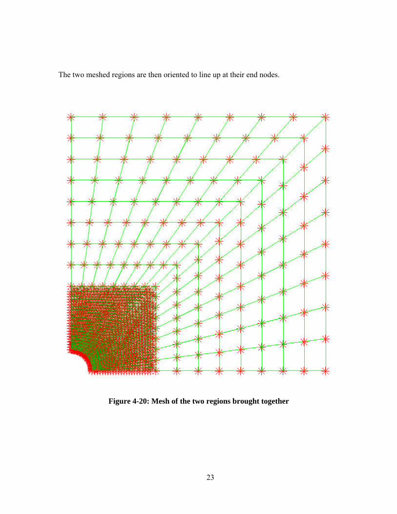
The two meshed regions are then oriented to line up at their end nodes.

Figure 4-20: Mesh of the two regions brought together

23

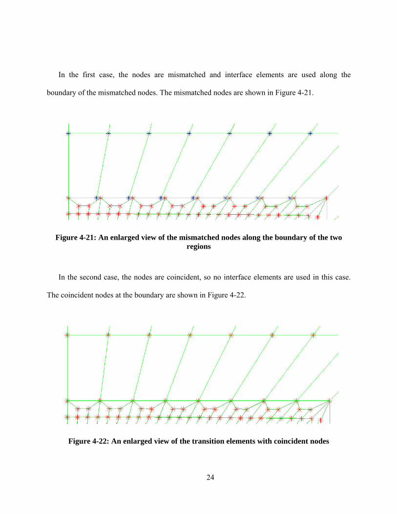
In the first case, the nodes are mismatched and interface elements are used along the

boundary of the mismatched nodes. The mismatched nodes are shown in Figure 4-21.

Figure 4-21: An enlarged view of the mismatched nodes along the boundary of the two regions

In the second case, the nodes are coincident, so no interface elements are used in this case.

The coincident nodes at the boundary are shown in Figure 4-22.

Figure 4-22: An enlarged view of the transition elements with coincident nodes

24

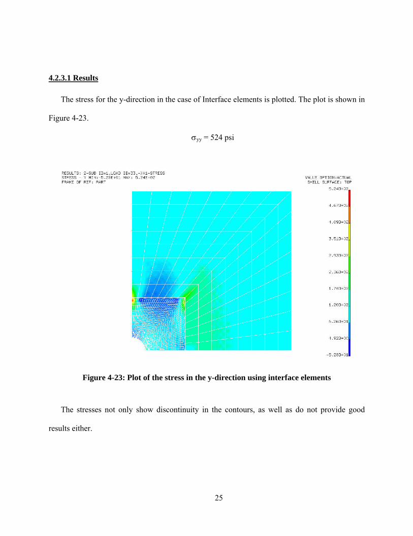
4.2.3.1 Results

The stress for the y-direction in the case of Interface elements is plotted. The plot is shown in

Figure 4-23.

σyy = 524 psi

Figure 4-23: Plot of the stress in the y-direction using interface elements

The stresses not only show discontinuity in the contours, as well as do not provide good

results either.

25

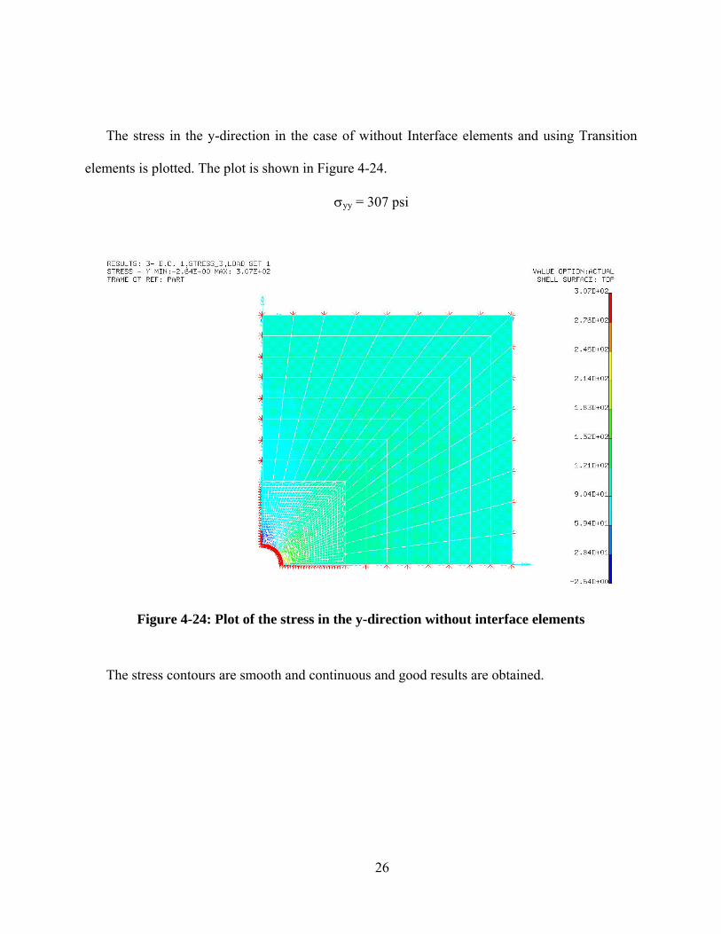
The stress in the y-direction in the case of without Interface elements and using Transition

elements is plotted. The plot is shown in Figure 4-24.

σyy = 307 psi

Figure 4-24: Plot of the stress in the y-direction without interface elements

The stress contours are smooth and continuous and good results are obtained.

26

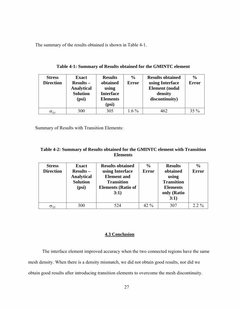
The summary of the results obtained is shown in Table 4-1.

Table 4-1: Summary of Results obtained for the GMINTC element

Stress Direction

Exact Results –

Analytical Solution

(psi)

Results obtained

using Interface Elements

(psi)

% Error

Results obtained using Interface Element (nodal

density discontinuity)

% Error

σyy 300 305 1.6 % 462 35 %

Summary of Results with Transition Elements:

Table 4-2: Summary of Results obtained for the GMINTC element with Transition Elements

Stress

Direction Exact

Results – Analytical Solution

(psi)

Results obtained using Interface Element and Transition

Elements (Ratio of 3:1)

% Error

Results obtained

using Transition Elements

only (Ratio 3:1)

% Error

σyy 300 524 42 % 307 2.2 %

4.3 Conclusion

The interface element improved accuracy when the two connected regions have the same

mesh density. When there is a density mismatch, we did not obtain good results, nor did we

obtain good results after introducing transition elements to overcome the mesh discontinuity.

27

CHAPTER 5 SHELL-TO-SOLID INTERFACE ELEMENTS

5.1 Introduction

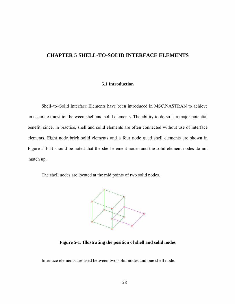
Shell–to–Solid Interface Elements have been introduced in MSC.NASTRAN to achieve

an accurate transition between shell and solid elements. The ability to do so is a major potential

benefit, since, in practice, shell and solid elements are often connected without use of interface

elements. Eight node brick solid elements and a four node quad shell elements are shown in

Figure 5-1. It should be noted that the shell element nodes and the solid element nodes do not

'match up'.

The shell nodes are located at the mid points of two solid nodes.

Figure 5-1: Illustrating the position of shell and solid nodes

Interface elements are used between two solid nodes and one shell node.

28

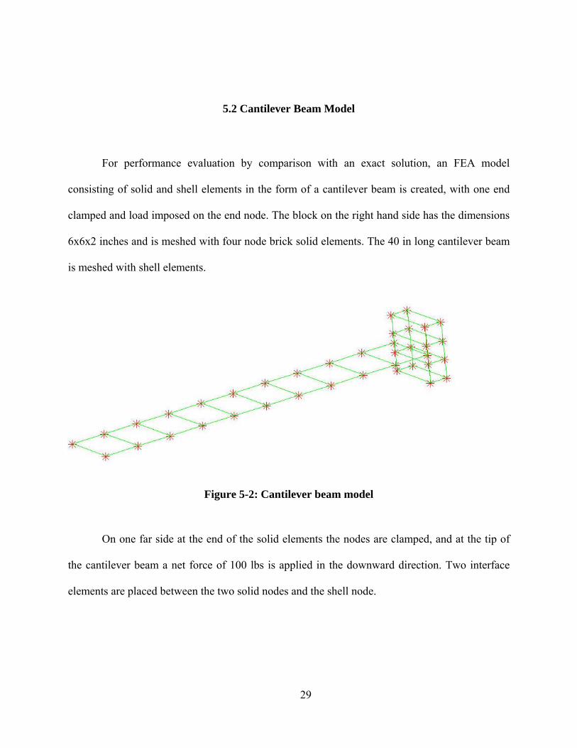
5.2 Cantilever Beam Model

For performance evaluation by comparison with an exact solution, an FEA model

consisting of solid and shell elements in the form of a cantilever beam is created, with one end

clamped and load imposed on the end node. The block on the right hand side has the dimensions

6x6x2 inches and is meshed with four node brick solid elements. The 40 in long cantilever beam

is meshed with shell elements.

Figure 5-2: Cantilever beam model

On one far side at the end of the solid elements the nodes are clamped, and at the tip of

the cantilever beam a net force of 100 lbs is applied in the downward direction. Two interface

elements are placed between the two solid nodes and the shell node.

29

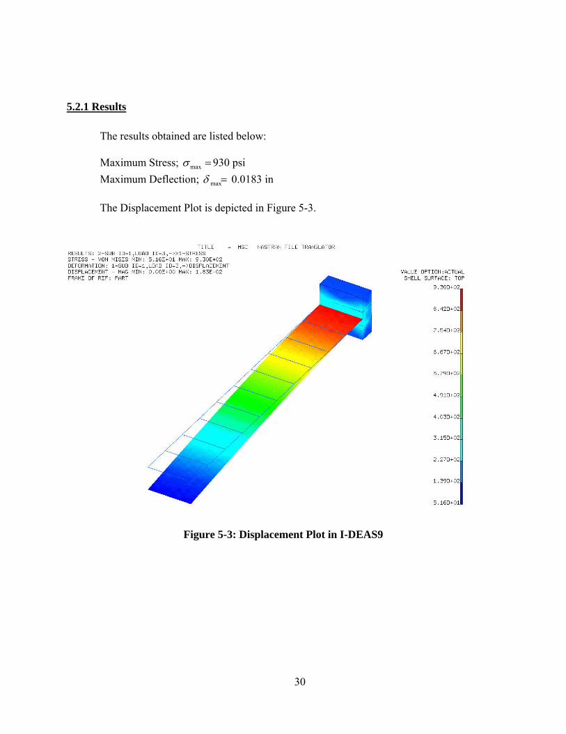
5.2.1 Results

The results obtained are listed below:

Maximum Stress; =maxσ 930 psi Maximum Deflection; =maxδ 0.0183 in

The Displacement Plot is depicted in Figure 5-3.

Figure 5-3: Displacement Plot in I-DEAS9

30

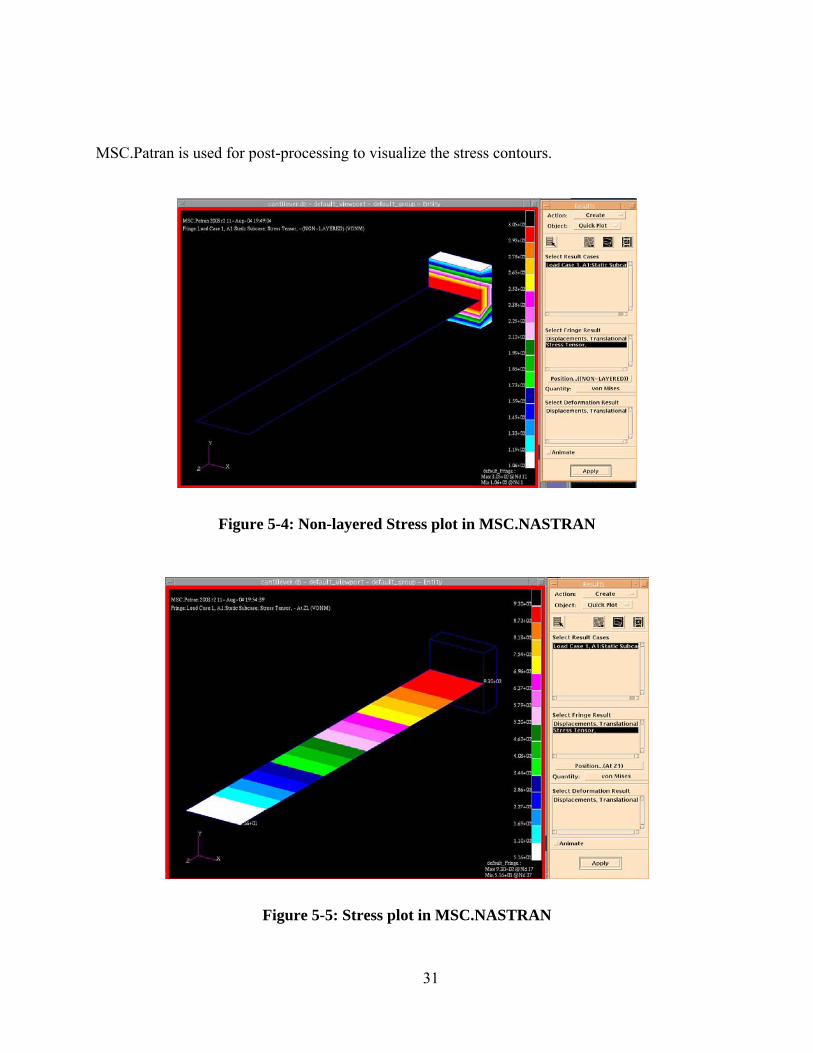
MSC.Patran is used for post-processing to visualize the stress contours.

Figure 5-4: Non-layered Stress plot in MSC.NASTRAN

Figure 5-5: Stress plot in MSC.NASTRAN

31

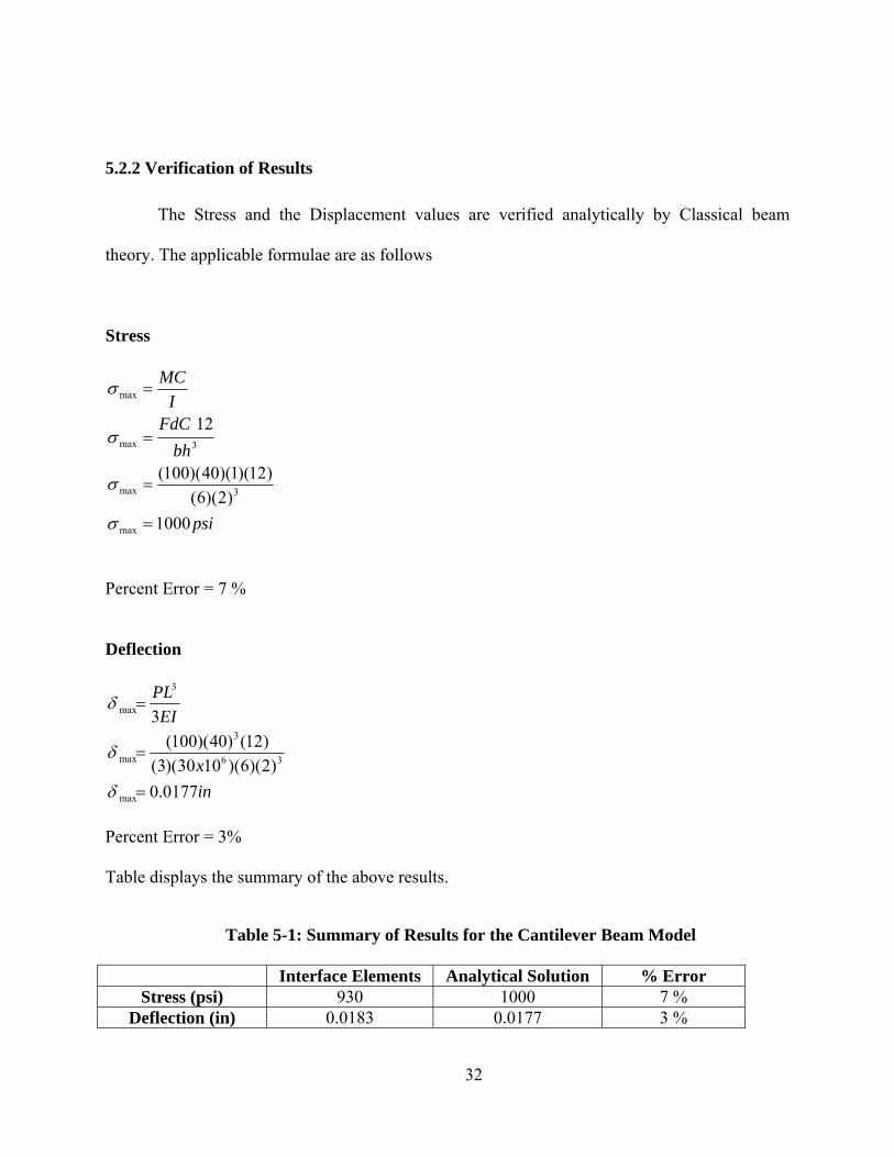
5.2.2 Verification of Results

The Stress and the Displacement values are verified analytically by Classical beam

theory. The applicable formulae are as follows

Stress

psi

bhFdC

IMC

1000)2)(6(

)12)(1)(40)(100(

12

max

3max

3max

max

=

=

=

=

σ

σ

σ

σ

Percent Error = 7 % Deflection

inx

EIPL

0177.0)2)(6)(1030)(3(

)12()40)(100(3

max

36

3

max

3

max

=

=

=

δ

δ

δ

Percent Error = 3% Table displays the summary of the above results.

Table 5-1: Summary of Results for the Cantilever Beam Model

Interface Elements Analytical Solution % Error Stress (psi) 930 1000 7 %

Deflection (in) 0.0183 0.0177 3 %

32

5.3 Quarter Plate Model

The quarter plate discussed in the earlier chapter is again invoked for the RSSCON

(shell-solid interface element). Here, three cases as follows are presented.

Case 1: a = 0.5, b = 0.5 Case 2: a = 0.25, b = 0.5 Case 3: a = 0.05, b = 0.5

where, ‘b’ and ‘a’ are the major and minor axes to the circular/elliptical hole in the center of the

12 x 12 inch symmetric plate. Note that the ellipse approximates a crack in Case 3.

As earlier, owing to symmetry the quarter plate is meshed and symmetric conditions are

applied to the two edges of the plate. A force of 25 lbs is applied on the top edge of the plate, and

isotropic steel material properties are used.

5.3.1Quarter Plate Model - Case 1

The 6 x 6 in quarter plate with a center hole cut-out of 0.5 in radius is shown in Figure 5-

6.

33

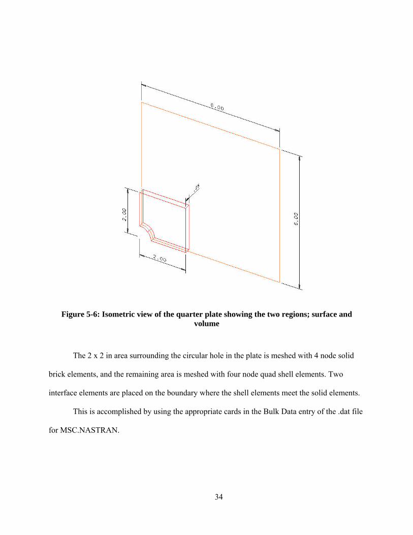
Figure 5-6: Isometric view of the quarter plate showing the two regions; surface and volume

The 2 x 2 in area surrounding the circular hole in the plate is meshed with 4 node solid

brick elements, and the remaining area is meshed with four node quad shell elements. Two

interface elements are placed on the boundary where the shell elements meet the solid elements.

This is accomplished by using the appropriate cards in the Bulk Data entry of the .dat file

for MSC.NASTRAN.

34

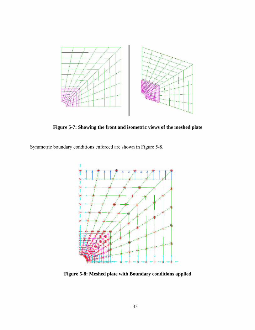
Figure 5-7: Showing the front and isometric views of the meshed plate Symmetric boundary conditions enforced are shown in Figure 5-8.

Figure 5-8: Meshed plate with Boundary conditions applied

35

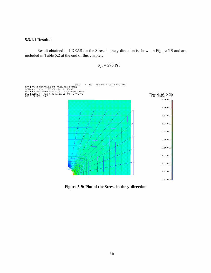
5.3.1.1 Results

Result obtained in I-DEAS for the Stress in the y-direction is shown in Figure 5-9 and are included in Table 5.2 at the end of this chapter.

σyy = 296 Psi

Figure 5-9: Plot of the Stress in the y-direction

36

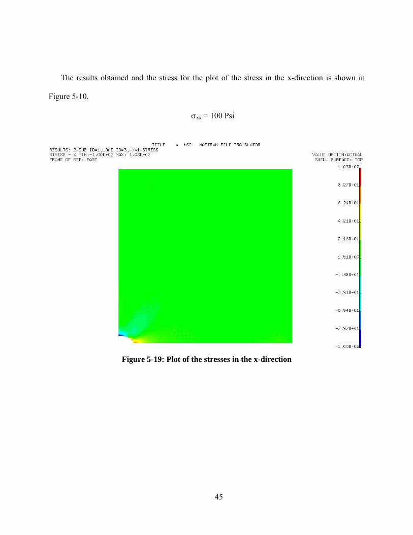
The results obtained and the stress for the plot of the stress in the x-direction is shown in

Figure 5-10.

σxx = 90 Psi

Figure 5-10: Plot of the stress in the x-direction

37

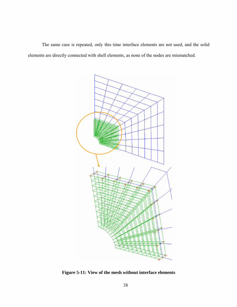
The same case is repeated, only this time interface elements are not used, and the solid

elements are directly connected with shell elements, as none of the nodes are mismatched.

Figure 5-11: View of the mesh without interface elements

38

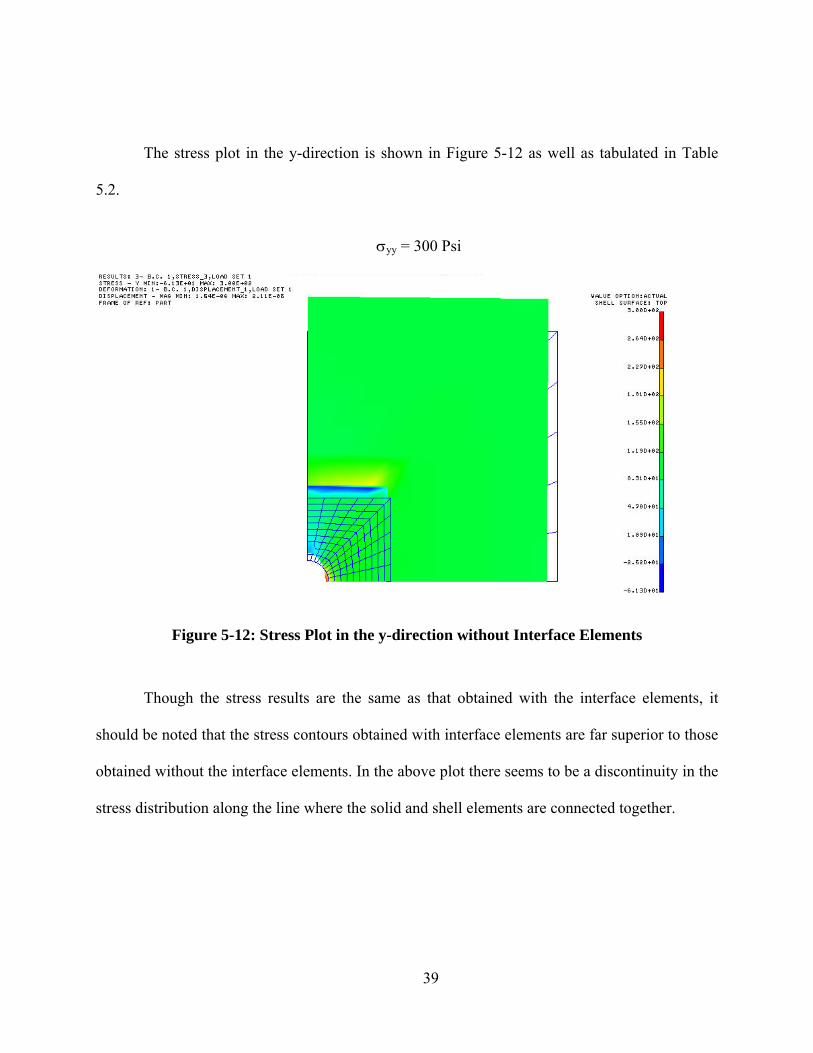
The stress plot in the y-direction is shown in Figure 5-12 as well as tabulated in Table

5.2.

σyy = 300 Psi

Figure 5-12: Stress Plot in the y-direction without Interface Elements

Though the stress results are the same as that obtained with the interface elements, it

should be noted that the stress contours obtained with interface elements are far superior to those

obtained without the interface elements. In the above plot there seems to be a discontinuity in the

stress distribution along the line where the solid and shell elements are connected together.

39

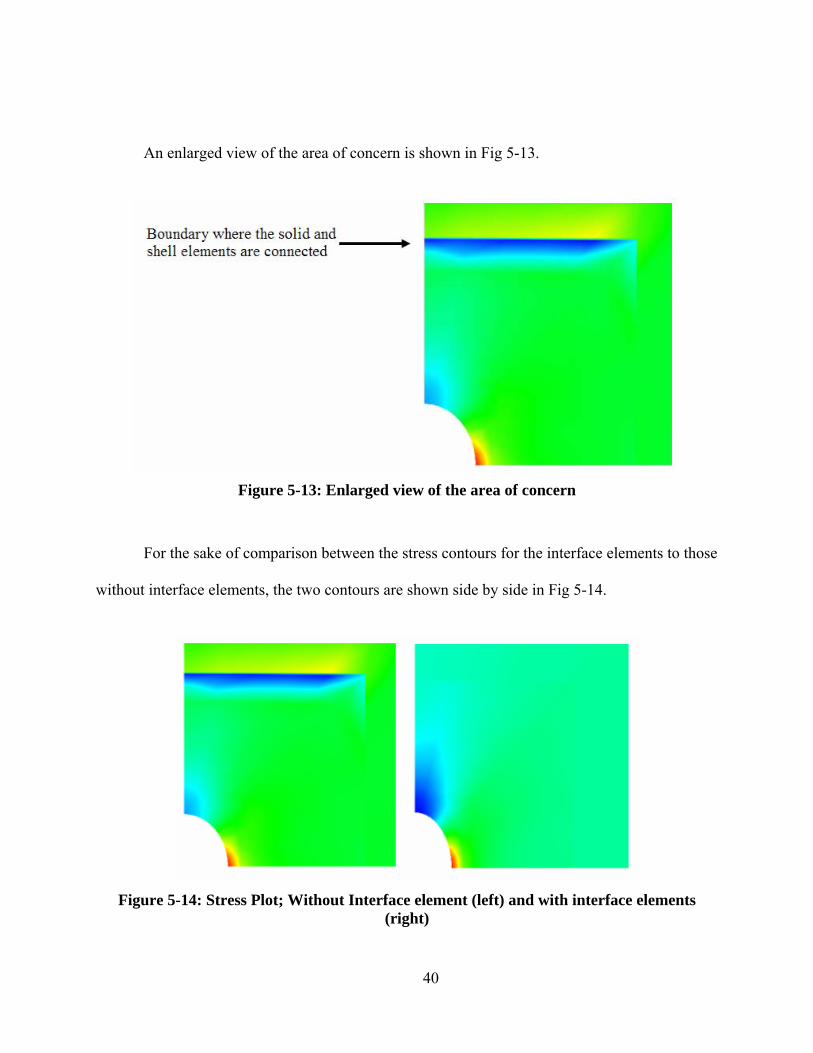
An enlarged view of the area of concern is shown in Fig 5-13.

Figure 5-13: Enlarged view of the area of concern

For the sake of comparison between the stress contours for the interface elements to those

without interface elements, the two contours are shown side by side in Fig 5-14.

Figure 5-14: Stress Plot; Without Interface element (left) and with interface elements

(right)

40

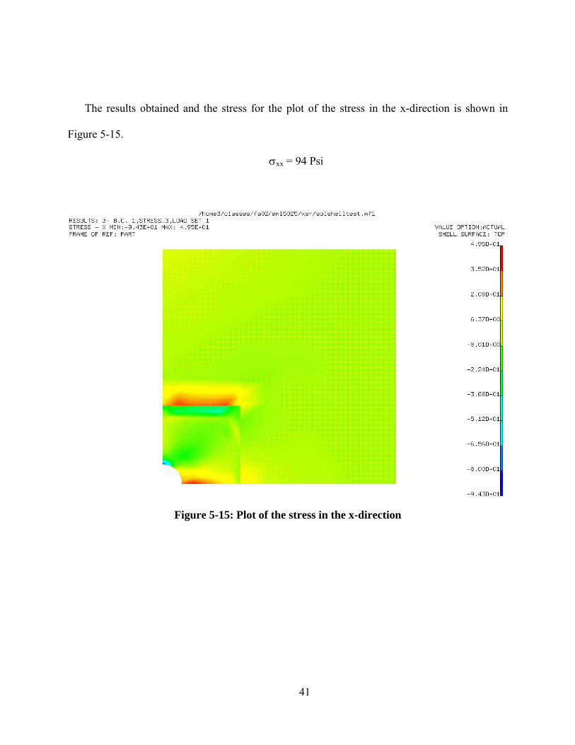
The results obtained and the stress for the plot of the stress in the x-direction is shown in

Figure 5-15.

σxx = 94 Psi

Figure 5-15: Plot of the stress in the x-direction

41

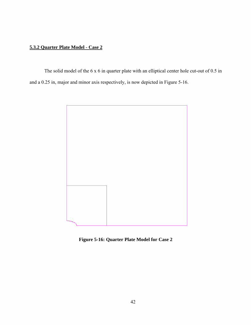
5.3.2 Quarter Plate Model - Case 2

The solid model of the 6 x 6 in quarter plate with an elliptical center hole cut-out of 0.5 in

and a 0.25 in, major and minor axis respectively, is now depicted in Figure 5-16.

Figure 5-16: Quarter Plate Model for Case 2

42

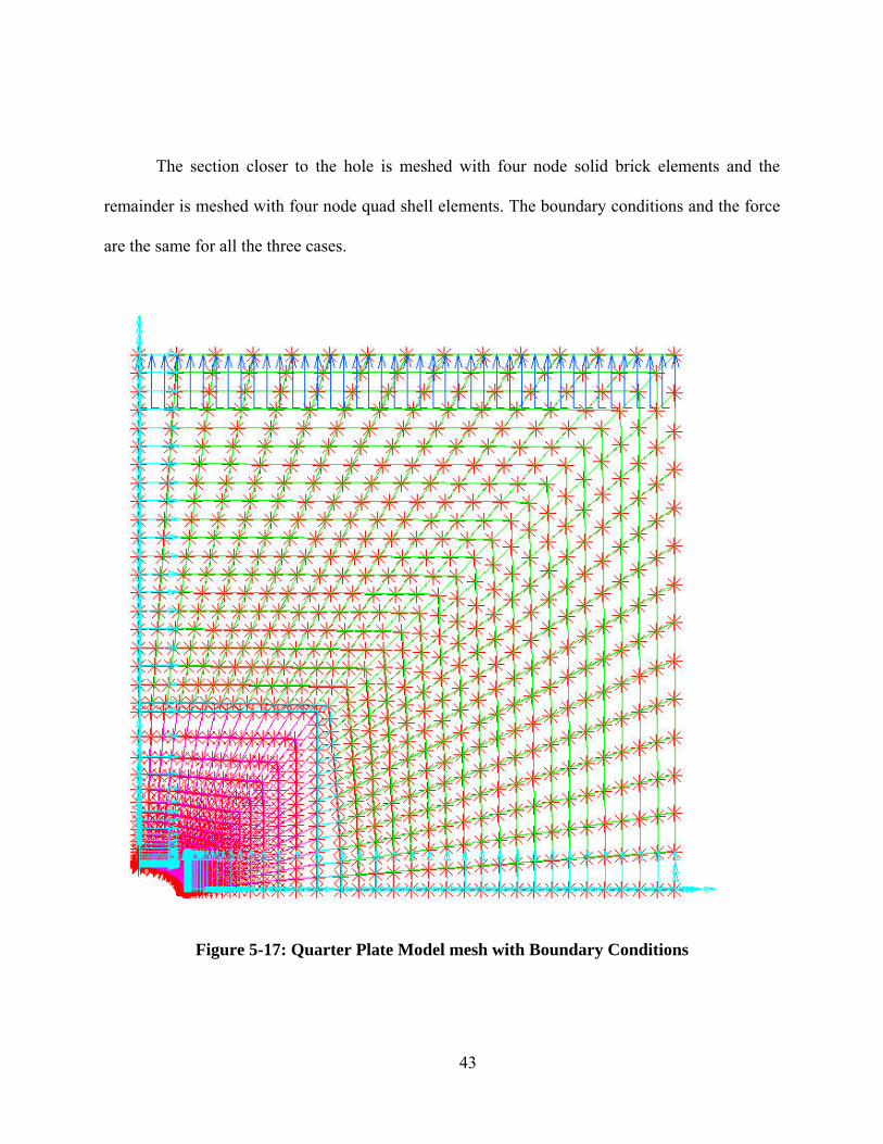
The section closer to the hole is meshed with four node solid brick elements and the

remainder is meshed with four node quad shell elements. The boundary conditions and the force

are the same for all the three cases.

Figure 5-17: Quarter Plate Model mesh with Boundary Conditions

43

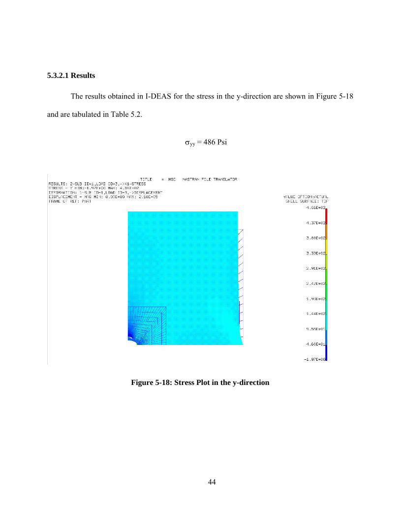
5.3.2.1 Results

The results obtained in I-DEAS for the stress in the y-direction are shown in Figure 5-18

and are tabulated in Table 5.2.

σyy = 486 Psi

Figure 5-18: Stress Plot in the y-direction

44

The results obtained and the stress for the plot of the stress in the x-direction is shown in

Figure 5-10.

σxx = 100 Psi

Figure 5-19: Plot of the stresses in the x-direction

45

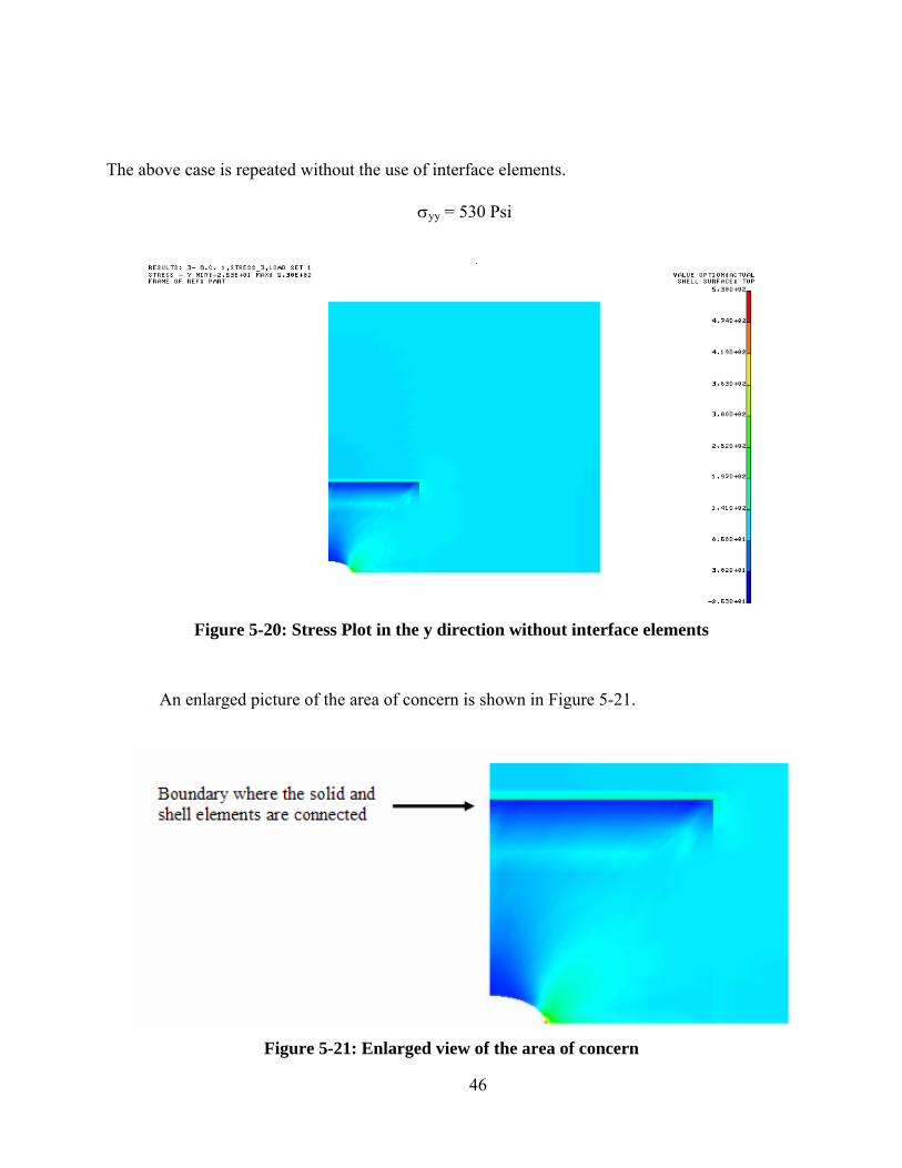
The above case is repeated without the use of interface elements.

σyy = 530 Psi

Figure 5-20: Stress Plot in the y direction without interface elements

An enlarged picture of the area of concern is shown in Figure 5-21.

Figure 5-21: Enlarged view of the area of concern

46

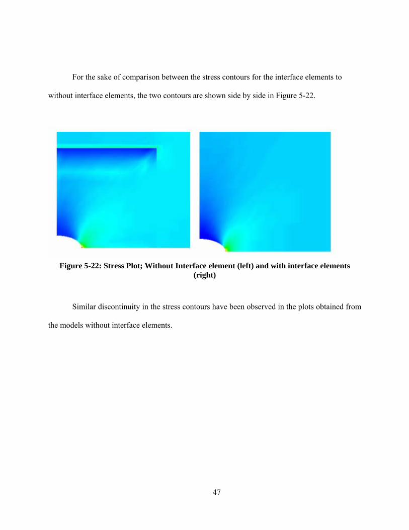
For the sake of comparison between the stress contours for the interface elements to

without interface elements, the two contours are shown side by side in Figure 5-22.

Figure 5-22: Stress Plot; Without Interface element (left) and with interface elements

(right)

Similar discontinuity in the stress contours have been observed in the plots obtained from

the models without interface elements.

47

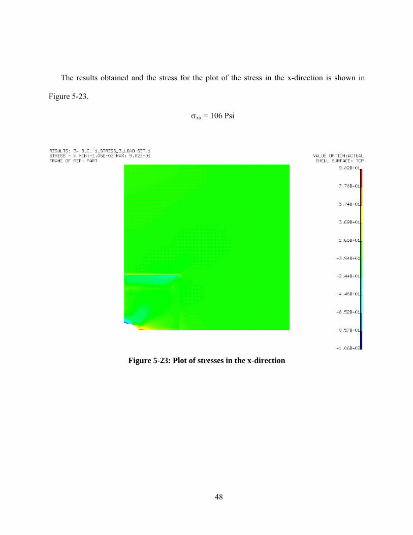
The results obtained and the stress for the plot of the stress in the x-direction is shown in

Figure 5-23.

σxx = 106 Psi

Figure 5-23: Plot of stresses in the x-direction

48

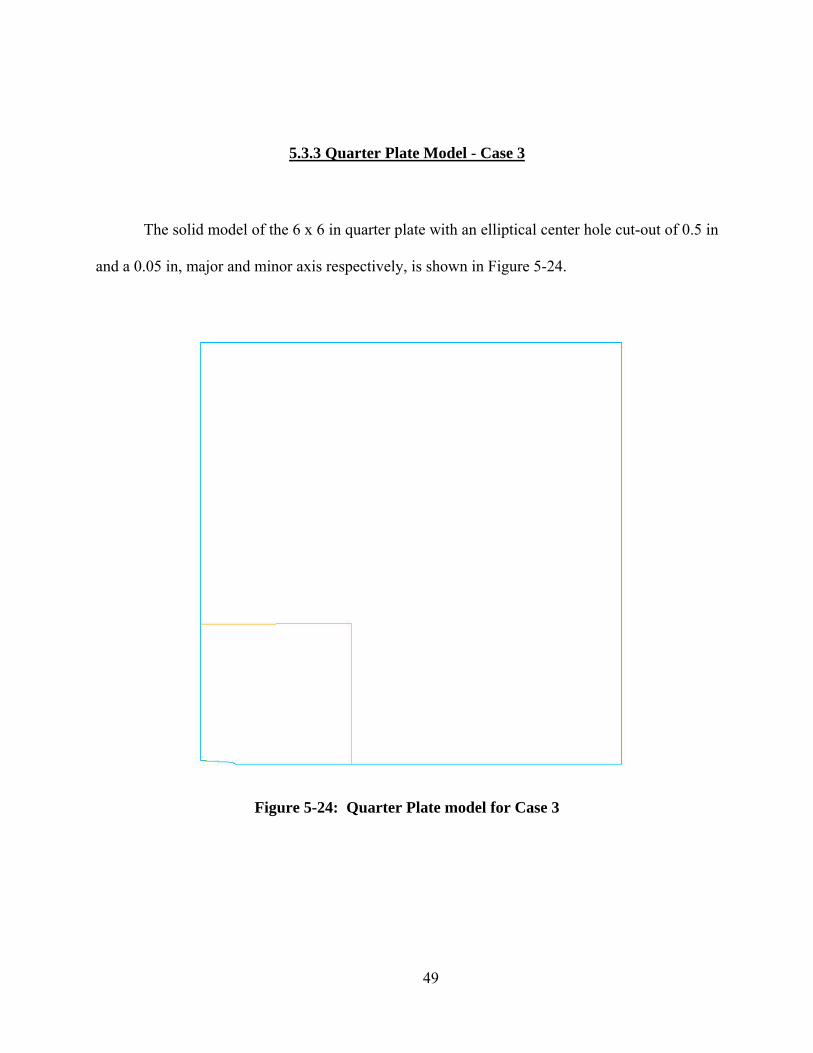
5.3.3 Quarter Plate Model - Case 3

The solid model of the 6 x 6 in quarter plate with an elliptical center hole cut-out of 0.5 in

and a 0.05 in, major and minor axis respectively, is shown in Figure 5-24.

Figure 5-24: Quarter Plate model for Case 3

49

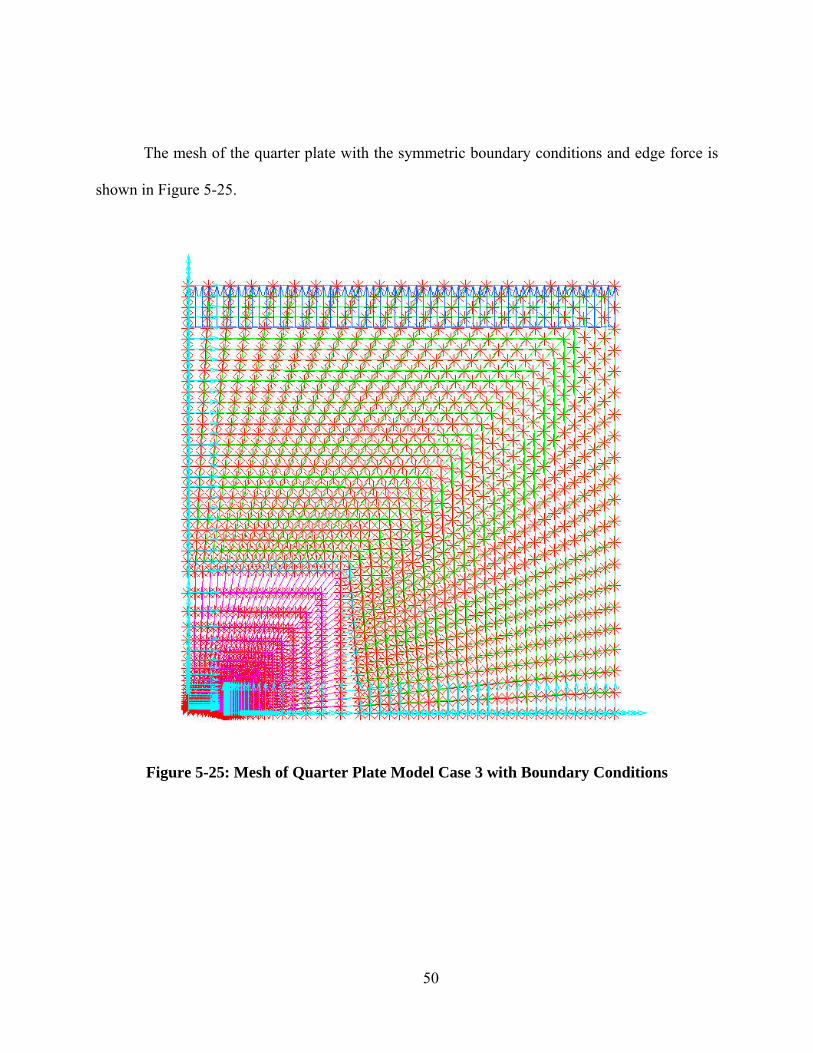
The mesh of the quarter plate with the symmetric boundary conditions and edge force is

shown in Figure 5-25.

Figure 5-25: Mesh of Quarter Plate Model Case 3 with Boundary Conditions

50

5.3.3.1 Results

The result obtained in I-DEAS for the stress in the y-direction is depicted in Figure 5-26,

and listed in Table 5.2.

σyy = 2160 Psi

Figure 5-26: Stress plot in the y-direction

51

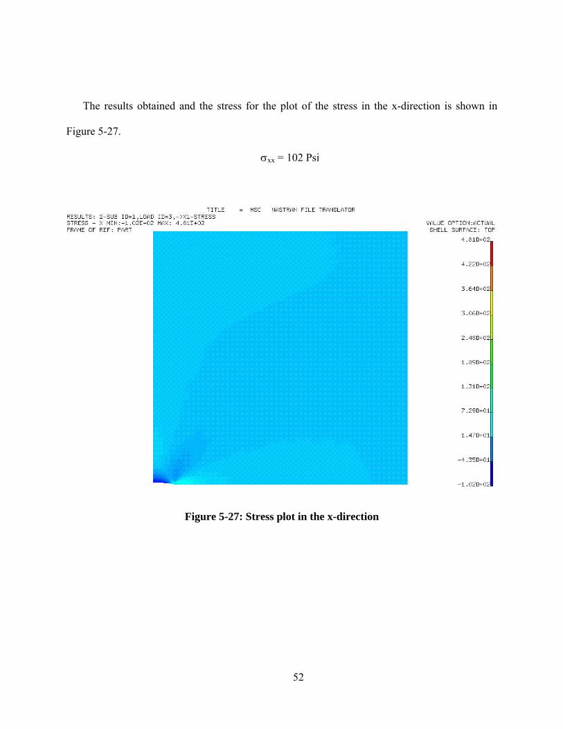
The results obtained and the stress for the plot of the stress in the x-direction is shown in

Figure 5-27.

σxx = 102 Psi

Figure 5-27: Stress plot in the x-direction

52

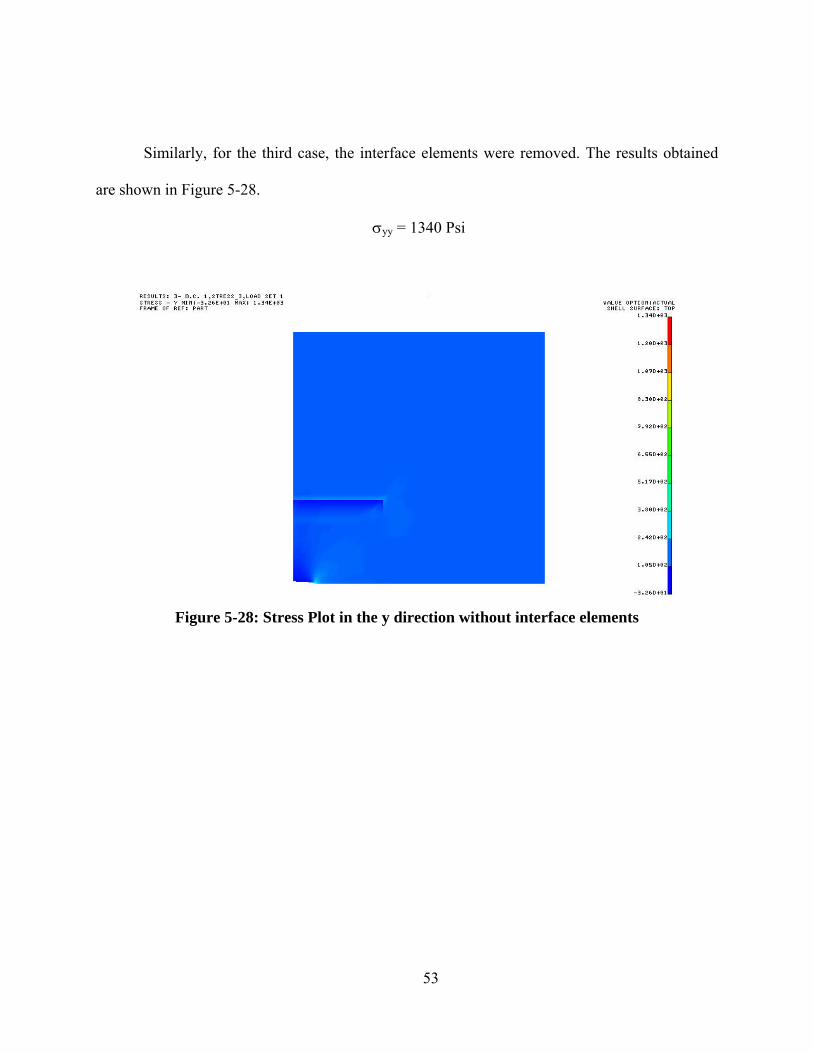
Similarly, for the third case, the interface elements were removed. The results obtained

are shown in Figure 5-28.

σyy = 1340 Psi

Figure 5-28: Stress Plot in the y direction without interface elements

53

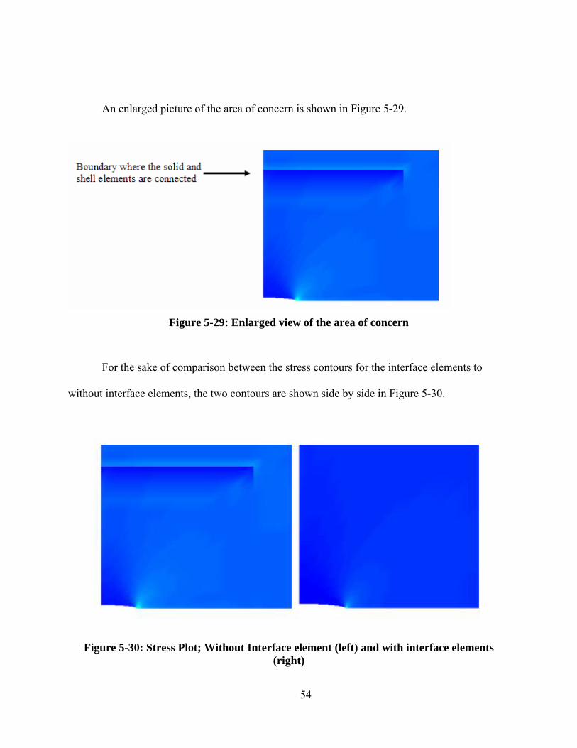
An enlarged picture of the area of concern is shown in Figure 5-29.

Figure 5-29: Enlarged view of the area of concern

For the sake of comparison between the stress contours for the interface elements to

without interface elements, the two contours are shown side by side in Figure 5-30.

Figure 5-30: Stress Plot; Without Interface element (left) and with interface elements (right)

54

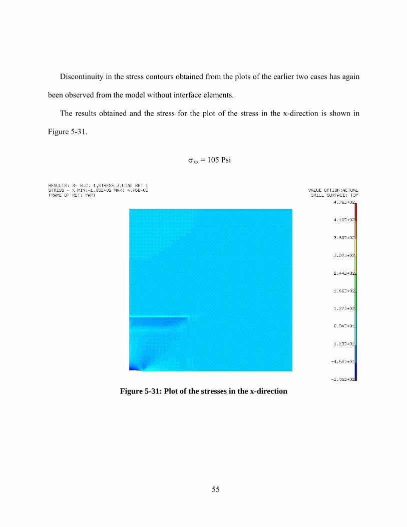
Discontinuity in the stress contours obtained from the plots of the earlier two cases has again

been observed from the model without interface elements.

The results obtained and the stress for the plot of the stress in the x-direction is shown in

Figure 5-31.

σxx = 105 Psi

Figure 5-31: Plot of the stresses in the x-direction

55

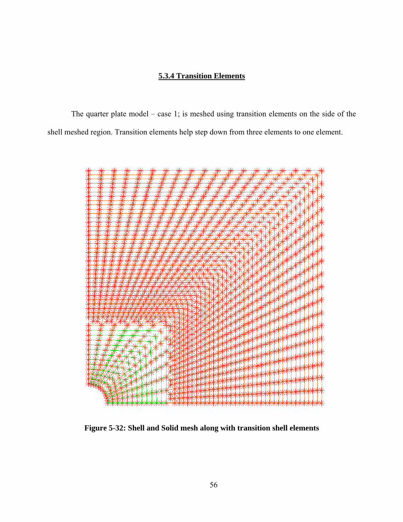
5.3.4 Transition Elements

The quarter plate model – case 1; is meshed using transition elements on the side of the

shell meshed region. Transition elements help step down from three elements to one element.

Figure 5-32: Shell and Solid mesh along with transition shell elements

56

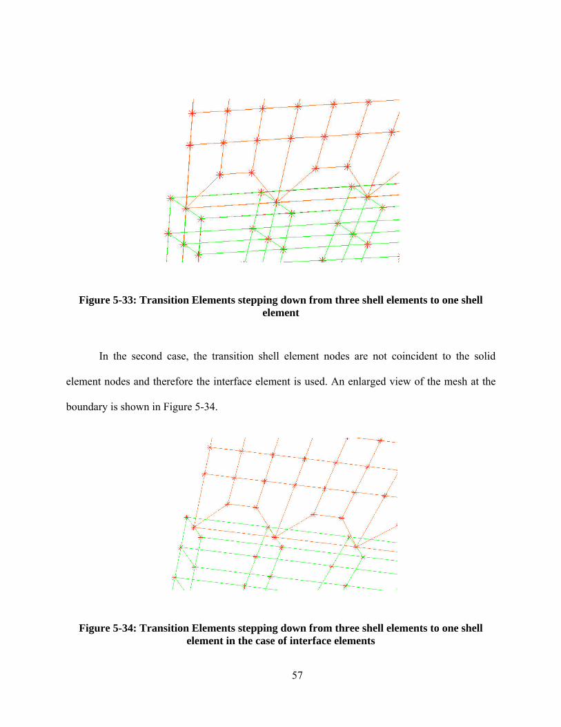
Figure 5-33: Transition Elements stepping down from three shell elements to one shell element

In the second case, the transition shell element nodes are not coincident to the solid

element nodes and therefore the interface element is used. An enlarged view of the mesh at the

boundary is shown in Figure 5-34.

Figure 5-34: Transition Elements stepping down from three shell elements to one shell element in the case of interface elements

57

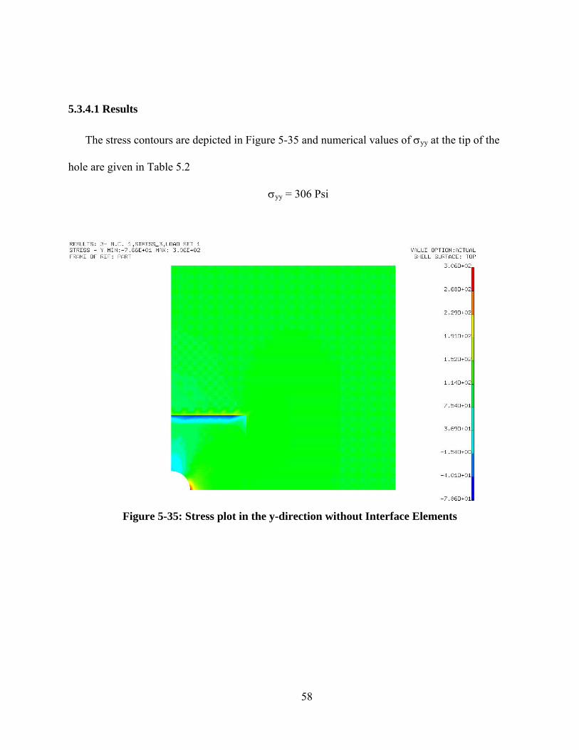
5.3.4.1 Results

The stress contours are depicted in Figure 5-35 and numerical values of σyy at the tip of the

hole are given in Table 5.2

σyy = 306 Psi

Figure 5-35: Stress plot in the y-direction without Interface Elements

58

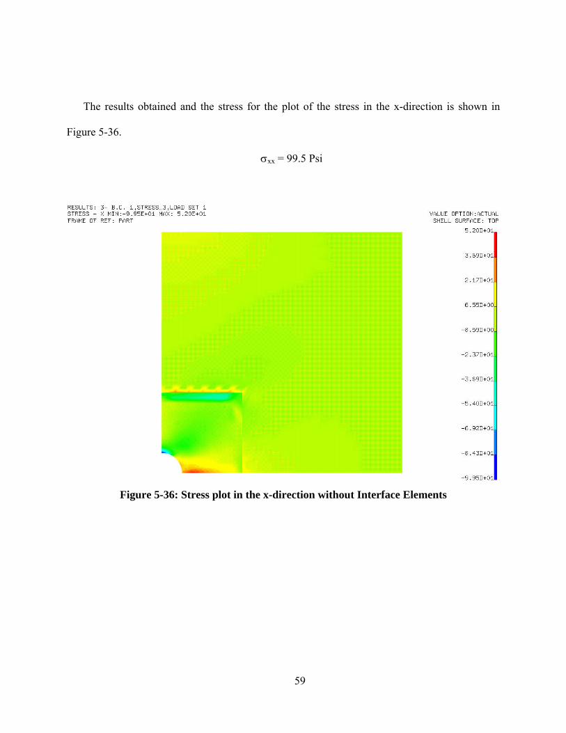
The results obtained and the stress for the plot of the stress in the x-direction is shown in

Figure 5-36.

σxx = 99.5 Psi

Figure 5-36: Stress plot in the x-direction without Interface Elements

59

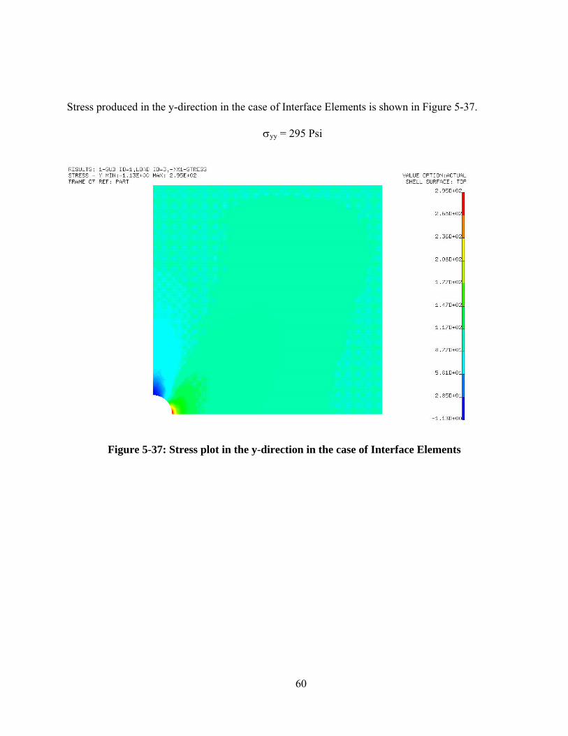
Stress produced in the y-direction in the case of Interface Elements is shown in Figure 5-37.

σyy = 295 Psi

Figure 5-37: Stress plot in the y-direction in the case of Interface Elements

60

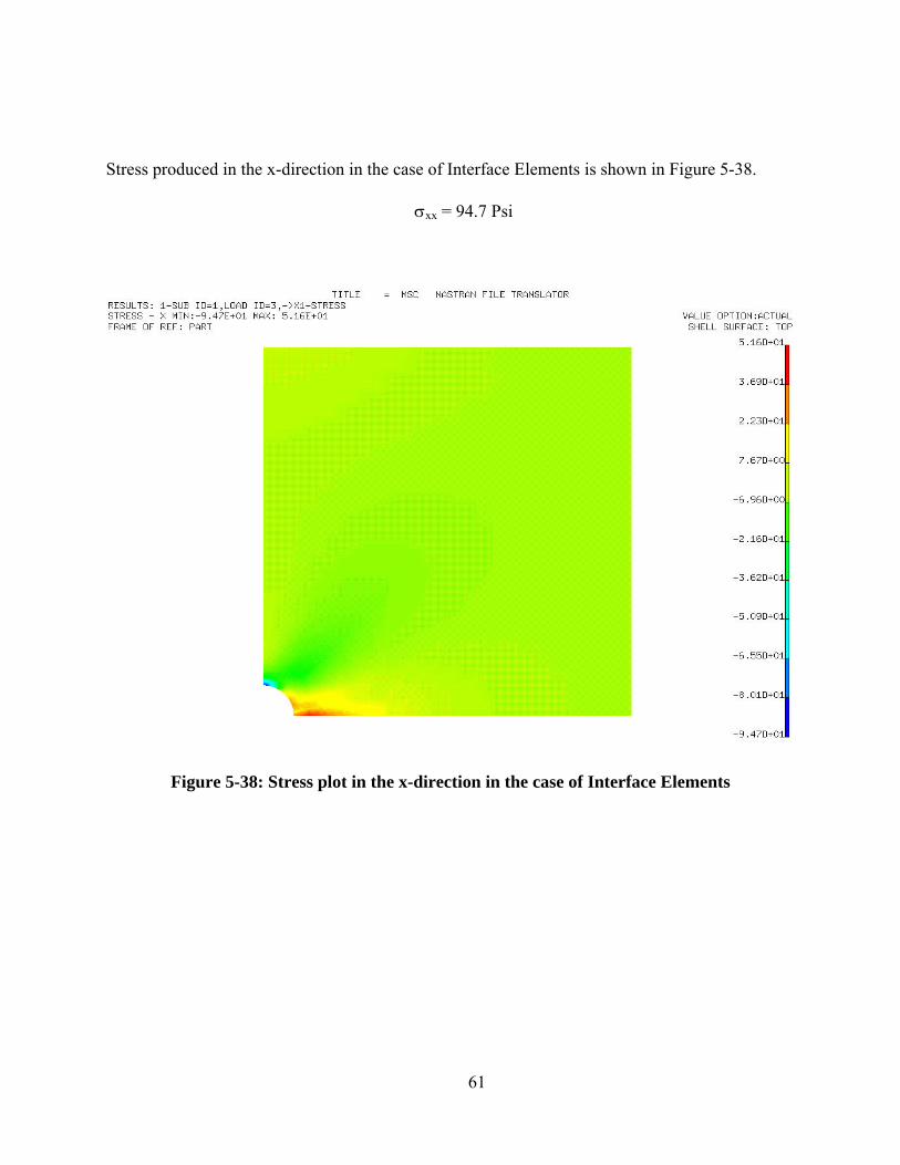
Stress produced in the x-direction in the case of Interface Elements is shown in Figure 5-38.

σxx = 94.7 Psi

Figure 5-38: Stress plot in the x-direction in the case of Interface Elements

61

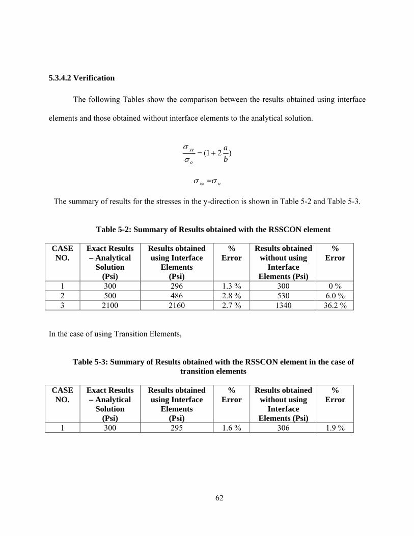
5.3.4.2 Verification

The following Tables show the comparison between the results obtained using interface

elements and those obtained without interface elements to the analytical solution.

)21(ba

o

yy +=σσ

oxx σσ =

The summary of results for the stresses in the y-direction is shown in Table 5-2 and Table 5-3.

Table 5-2: Summary of Results obtained with the RSSCON element

CASE NO.

Exact Results – Analytical

Solution (Psi)

Results obtained using Interface

Elements (Psi)

% Error

Results obtained without using

Interface Elements (Psi)

% Error

1 300 296 1.3 % 300 0 % 2 500 486 2.8 % 530 6.0 % 3 2100 2160 2.7 % 1340 36.2 %

In the case of using Transition Elements,

Table 5-3: Summary of Results obtained with the RSSCON element in the case of transition elements

CASE NO.

Exact Results – Analytical

Solution (Psi)

Results obtained using Interface

Elements (Psi)

% Error

Results obtained without using

Interface Elements (Psi)

% Error

1 300 295 1.6 % 306 1.9 %

62

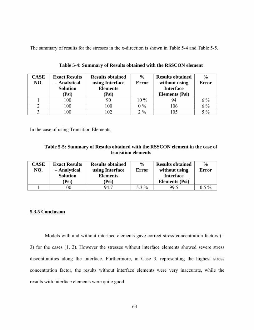
The summary of results for the stresses in the x-direction is shown in Table 5-4 and Table 5-5.

Table 5-4: Summary of Results obtained with the RSSCON element CASE NO.

Exact Results – Analytical

Solution (Psi)

Results obtained using Interface

Elements (Psi)

% Error

Results obtained without using

Interface Elements (Psi)

% Error

1 100 90 10 % 94 6 % 2 100 100 0 % 106 6 % 3 100 102 2 % 105 5 %

In the case of using Transition Elements,

Table 5-5: Summary of Results obtained with the RSSCON element in the case of transition elements

CASE NO.

Exact Results – Analytical

Solution (Psi)

Results obtained using Interface

Elements (Psi)

% Error

Results obtained without using

Interface Elements (Psi)

% Error

1 100 94.7 5.3 % 99.5 0.5 %

5.3.5 Conclusion

Models with and without interface elements gave correct stress concentration factors (=

3) for the cases (1, 2). However the stresses without interface elements showed severe stress

discontinuities along the interface. Furthermore, in Case 3, representing the highest stress

concentration factor, the results without interface elements were very inaccurate, while the

results with interface elements were quite good.

63

For Case 1, the circle, using transition elements provided accurate results with and

without transition elements.

5.4 Non-linear Model

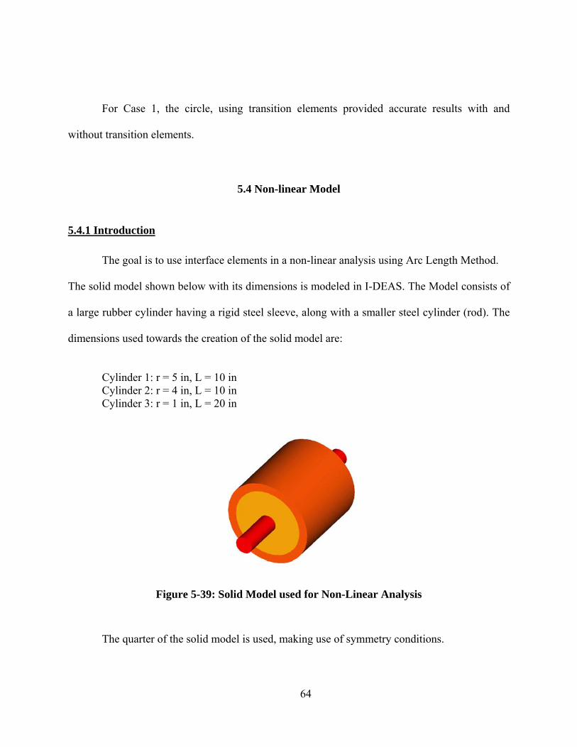
5.4.1 Introduction

The goal is to use interface elements in a non-linear analysis using Arc Length Method. The solid model shown below with its dimensions is modeled in I-DEAS. The Model consists of

a large rubber cylinder having a rigid steel sleeve, along with a smaller steel cylinder (rod). The

dimensions used towards the creation of the solid model are:

Cylinder 1: r = 5 in, L = 10 in Cylinder 2: r = 4 in, L = 10 in Cylinder 3: r = 1 in, L = 20 in

Figure 5-39: Solid Model used for Non-Linear Analysis

The quarter of the solid model is used, making use of symmetry conditions.

64

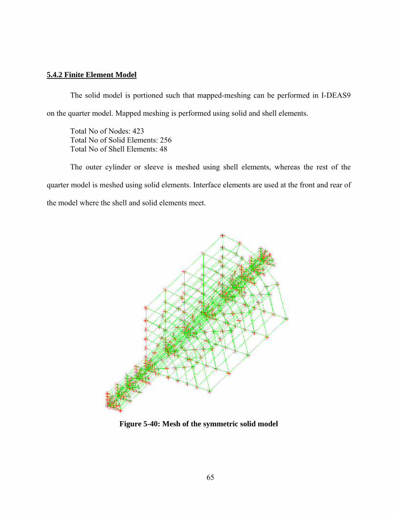
5.4.2 Finite Element Model

The solid model is portioned such that mapped-meshing can be performed in I-DEAS9

on the quarter model. Mapped meshing is performed using solid and shell elements.

Total No of Nodes: 423 Total No of Solid Elements: 256 Total No of Shell Elements: 48

The outer cylinder or sleeve is meshed using shell elements, whereas the rest of the

quarter model is meshed using solid elements. Interface elements are used at the front and rear of

the model where the shell and solid elements meet.

Figure 5-40: Mesh of the symmetric solid model

65

5.4.2.1 Material Properties:

5.4.2.1.1 Rubber

The Mooney-Rivlin rubber material properties are:

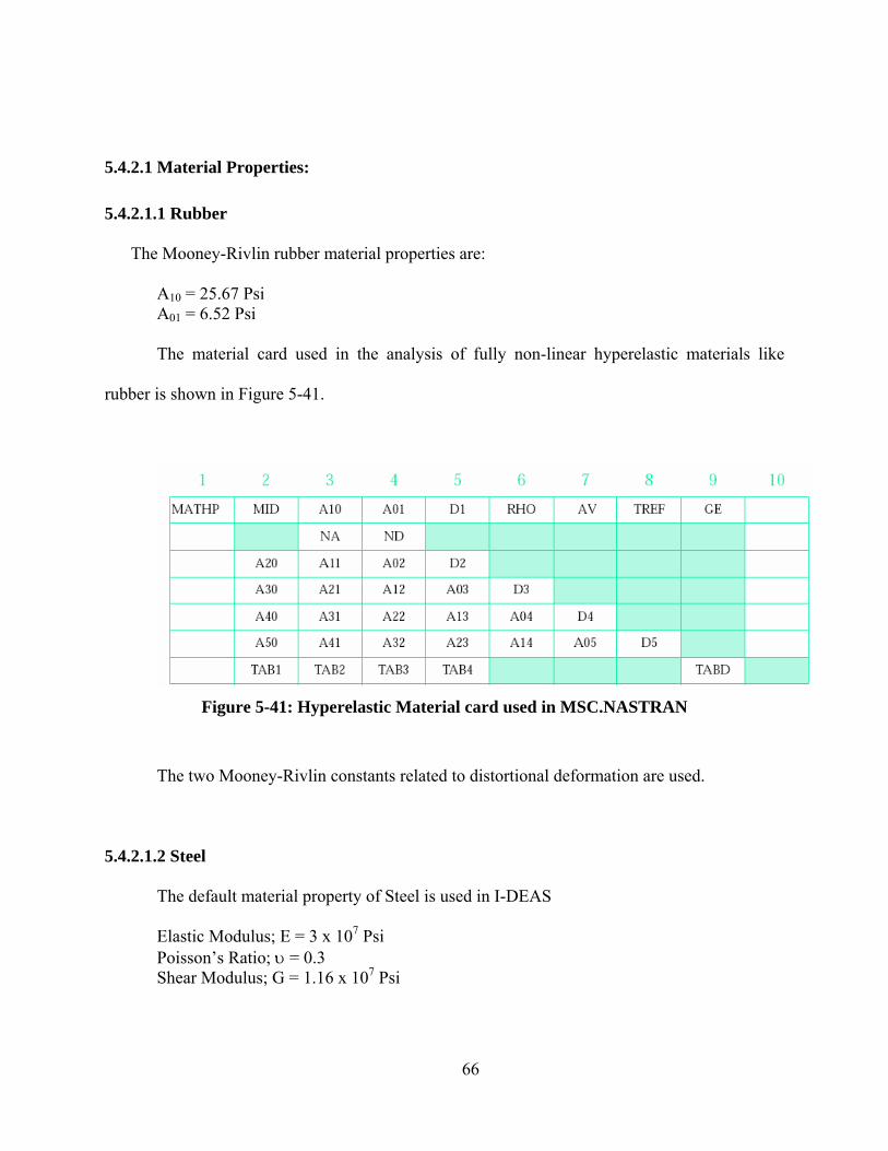
A10 = 25.67 Psi A01 = 6.52 Psi The material card used in the analysis of fully non-linear hyperelastic materials like

rubber is shown in Figure 5-41.

Figure 5-41: Hyperelastic Material card used in MSC.NASTRAN

The two Mooney-Rivlin constants related to distortional deformation are used.

5.4.2.1.2 Steel

The default material property of Steel is used in I-DEAS Elastic Modulus; E = 3 x 107 Psi Poisson’s Ratio; υ = 0.3 Shear Modulus; G = 1.16 x 107 Psi

66

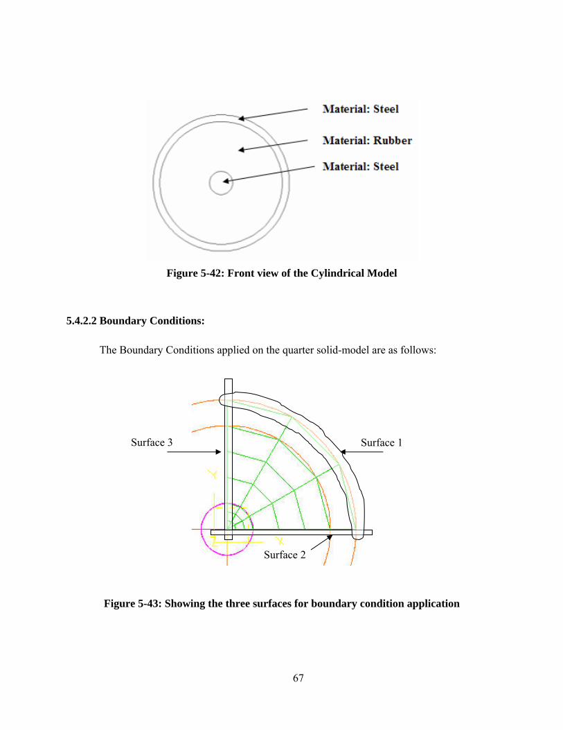
Figure 5-42: Front view of the Cylindrical Model

5.4.2.2 Boundary Conditions:

The Boundary Conditions applied on the quarter solid-model are as follows:

Surface 1

Surface 2

Surface 3

Figure 5-43: Showing the three surfaces for boundary condition application

67

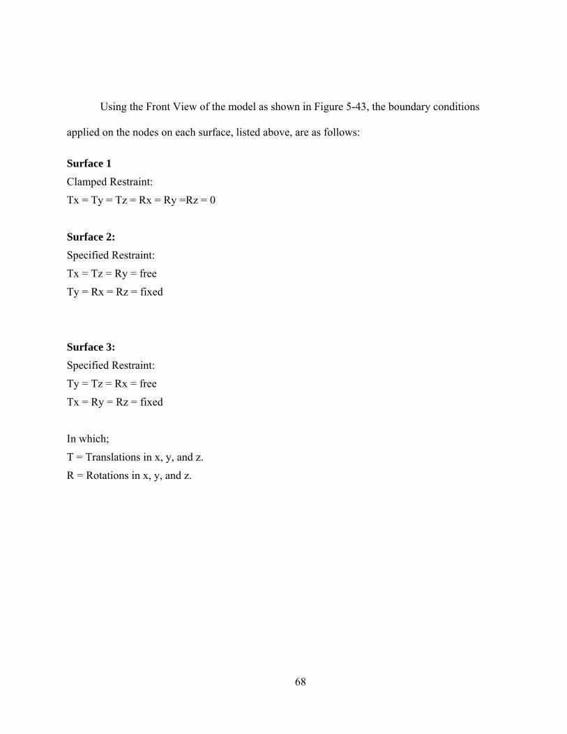
Using the Front View of the model as shown in Figure 5-43, the boundary conditions

applied on the nodes on each surface, listed above, are as follows:

Surface 1

Clamped Restraint:

Tx = Ty = Tz = Rx = Ry =Rz = 0

Surface 2:

Specified Restraint:

Tx = Tz = Ry = free

Ty = Rx = Rz = fixed

Surface 3: Specified Restraint:

Ty = Tz = Rx = free

Tx = Ry = Rz = fixed

In which;

T = Translations in x, y, and z.

R = Rotations in x, y, and z.

68

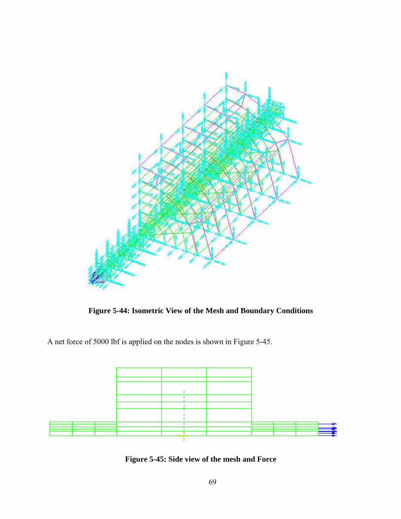
Figure 5-44: Isometric View of the Mesh and Boundary Conditions

A net force of 5000 lbf is applied on the nodes is shown in Figure 5-45.

Figure 5-45: Side view of the mesh and Force

69

5.4.2.3 I-DEAS9 to MSC.NASTRAN

After meshing, applying material properties, and boundary conditions, the FE model is

now exported from I-DEAS9 as a .DAT file.

The cards used for the non-linear analysis are as follows: “Executive Control” Section of the .DAT file: SOL 106 “Case Control” Section of the .DAT file: MPC = 1 NLPARM = 121 “Bulk Data” Section of the .DAT file: NLPARM 121 480 AUTO 1 YES NLPCI 121 CRIS 0.25 4.0 10000.0 1000000 50 MATHP 2 25.67 6.52

70

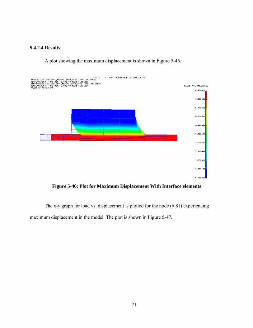
5.4.2.4 Results:

A plot showing the maximum displacement is shown in Figure 5-46.

Figure 5-46: Plot for Maximum Displacement With Interface elements

The x-y graph for load vs. displacement is plotted for the node (# 81) experiencing

maximum displacement in the model. The plot is shown in Figure 5-47.

71

Load vs. Displacement

0

1000

2000

3000

4000

5000

6000

0 1 2 3 4 5 6 7 8

Displacement

Load

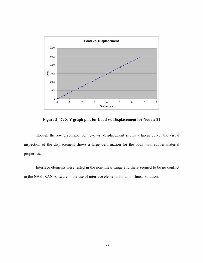
Figure 5-47: X-Y graph plot for Load vs. Displacement for Node # 81

Though the x-y graph plot for load vs. displacement shows a linear curve, the visual

inspection of the displacement shows a large deformation for the body with rubber material

properties.

Interface elements were tested in the non-linear range and there seemed to be no conflict

in the NASTRAN software in the use of interface elements for a non-linear solution.

72

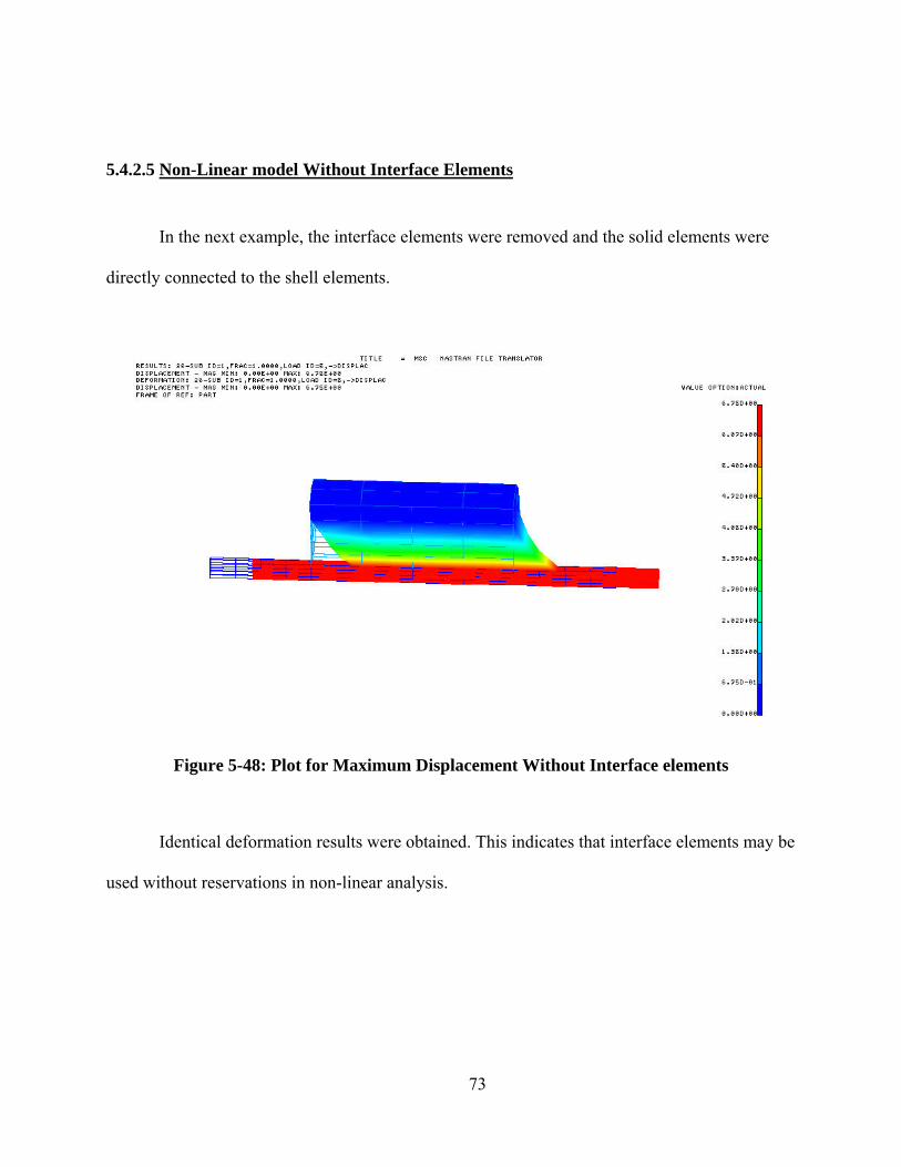
5.4.2.5 Non-Linear model Without Interface Elements

In the next example, the interface elements were removed and the solid elements were

directly connected to the shell elements.

Figure 5-48: Plot for Maximum Displacement Without Interface elements

Identical deformation results were obtained. This indicates that interface elements may be

used without reservations in non-linear analysis.

73

CHAPTER 6 DISCUSSION

The results obtained from the shell-shell interface element GMINTC for the quarter plate

model for the two regions having mismatched nodes show that when the regions have the same

number of elements in both the regions provide valid results. The stress values in the case of the

quarter plate model were verified by the analytical solution. In the case of interface elements

used at the boundary of a dense mesh to a coarse mesh, valid results were not obtained.

• In the case of the shell-to-solid interface element RSSCON, for the cantilever beam

model, the results obtained for the maximum stress and displacement were validated

analytically by classical beam theory.

• For three cases for the quarter plate model having solid elements in the area of the cut

and shell regions in the outer areas, the results were again compared with analytical

solution. The stress contours showed a good distribution along the interface which was

not achieved with the GMINTC element. Poor results were obtained in the sharp elliptical

hole when interface elements were not used, but very good results when they were.

• The interface elements were also used in a non-linear model having Mooney-Rivlin

rubber material properties and mismatched nodes. The interface elements gave the correct

answer, validating that they are applicable to nonlinear analysis.

74

• Interface elements for solid to shell elements were found to provide more accurate results

as compared to the interface elements for shell to shell elements.

• All boundary identification numbers must be unique.

• Interface elements may generate high or negative matrix/factor diagonal ratios. If there

are no other modeling errors, these messages may be ignored and PARAM, BAILOUT,-1

may be used to continue the run, although this is highly discouraged, and this parameter

was not used in any of the analyses carried out.

6.1 For the shell-to-shell interface element – GMINTC

The first and the last node on the interface boundary for two shell meshed regions should

be the same in the case of GMINTC element.

For the shell-to-shell interface element, three new cards were introduced in the Bulk Data

section, GMINC (Geometric Interface Curve), GMBNDC (Geometric Boundary Curve), and

PINTC (Properties of Geometric Interface Curve), where they define the interface curves, nodes

making up the boundary, and properties for the interface element.

The interface elements consists only of the difference in displacement components

weighted by Lagrange multipliers, there are no conventional element or material properties. For

the GMINTC element, the bulk data entry for property specifies a tolerance for the interface

75

element, which defines the allowable distance between the boundaries of the subdomains. If the

distance is greater than the tolerance value, a warning message will be issued.

Interface elements should be applied along a straight edge. If there is a 45 degree edge, two

interface elements should be used.

6.2 For the shell-to-solid interface element – RSSCON

For the shell-to-solid interface element, the RSSCON shell-solid element connector card is

introduced in the Bulk Data section. For every two solid element nodes, one shell element node

located in the middle is specified in this card.

The shell node musts lie between the two solid nodes for the RSSCON interface elements.

76

CHAPTER 7 CONCLUSION

The performance of interface elements was demonstrated in finite element methods on

different models for varied cases. The results obtained where then validated by analytical results,

and also each interface element model was compared to a similar model without using interface

elements.

Interface elements generally gave better results and smoother stress distributions

compared with not using interface elements when there were nodal or element mismatches.

We were not able to obtain accurate results when nodal density changes at a interface in

the case of shell-shell.

77

REFERENCES

Ansel C. Ugural and Saul K. Fenster, “Advanced Strength and Applied Elasticity”, 3rd Edition David Nicholson, “Finite Element Analysis Thermomechanics of solids” I-DEAS Online Help Bookshelf John E. Schiermeier, Jerrold M. Housner, M. A. Aminpour, W. Jefferson Stroud, “The application of interface elements to dissimilar meshes in global/local analysis” M.A. Aminpour, Jonathan B. Ransom, Susan L. McCleary, “A coupled analysis method for structures with independently modeled finite element subdomains” M.A. Aminpour, J.B. Ransom, and S.L. McCleary, “A New Interface Element for Connecting Independently Modeled Substructure” Michael Farley, “Redefining the Process of Airframe Finite Element Model Development using MSC/Super Model” MSC.NASTRAN Quick Reference Guide O.C. Zienkiewicz, “The Finite Element Method” Richard Zarda, “The Finite Element Method (FEM)” William F. Riley, Leroy D. Sturges, Don H. Morris, “Statics and Mechanics of Materials: An Integrated Approach”

78