t ~ E V I E R

An Intemational Joumal Available online at www.sciencedirect.com__ computers &

. c . . . c . ( - r ~ o , - • c T . m a t h e m a t i c s with applications

Computers and Mathematics with Applications 48 (2004) 995-1016 www.elsevier .com/locate/camwa

A Least Squares Coupl ing M e t h o d with Finite E lements and Boundary E l e m e n t s

for Transmiss ion Prob lems

M. MAISCHAK AND E. P. STEPHAN* Institut f/Jr Angewandte Mathematik

Universit£t Hannover Welfengarten 1, 30167 Hannover, Germany

<reals chak><st ephan>©if am. uni-hannover, de

A b s t r a c t - - W e analyze a least squares formulation for the numerical solution of second-order lin- ear transmission problems in two and three dimensions, which allow jumps on the interface. In a bounded domain the second-order partial differential equation is rewritten as a first-order system; the part of the transmission problem which corresponds to the unbounded exterior domain is refor- mulated by means of boundary integral equations on the interface. The least squares functional is given in terms of Sobolev norms of order -1 and of order 1/2. These norms are computed by approx- imating the corresponding inner products using multilevel preconditioners for a second-order elliptic problem in a bounded domain ~ and for the weakly singular integral operator of the single layer potential on its boundary 0~. As preconditioners we use both multigrid and BPX algorithms, and the preconditioned system has bounded or mildly growing condition number. Numerical experiments confirm our theoretical results. (~) 2004 Elsevier Ltd. All rights reserved.

K e y w o r d s - - L e a s t squares methods, Transmission problems, Finite elements, Boundary elements, Multilevel preconditioners.

1. I N T R O D U C T I O N

The coupling of finite elements and boundary elements has developed into a very powerful

method to tackle a large class of t ransmission problems in physics and engineering sciences

(see, e.g., [1-6]). In recent years an increasing interest evolved to apply mixed methods instead

of usual finite-element methods together with either boundary integral equations or Dirichlet-

to -Neumann mappings (see, e.g., [7-9]). Often in applications a mixed finite-element method is

more beneficial than the s tandard FEM, e.g., in s t ructural mechanics via mixed methods stresses

are computed more accurately than displacements. However, often in such mixed F E M / B E M

coupling methods it is difficult to work with finite-element spaces which satisfy appropriate dis-

crete inf-sup conditions. On the other hand, as it is well known, least squares formulations do

not require inf-sup conditions to be satisfied. Therefore they are especially a t t ract ive to use in

combinat ion with mixed formulations.

The use of variat ional methods of least squares type has been studied by many authors (see [10])

s tar t ing with the work by Bramble and Schatz [11]. One of the main least square methods

*This work was supported by the German Research Foundation (DFG) under Grant STE 573/3.

0898-1221/04/$ - see front matter (~ 2004 Elsevier Ltd. All rights reserved. doi: 10.1016/j.camwa.2004.10.002

Typeset by AA/~S-TF~

996 M. MAISCHAK AND E. P. STEPHAN

introduced by Stephan and Wendland [12], Wendland [13], and Jespersen [14] (see also [15]) uses the general theory of elliptic boundary value problems of Agmon-Douglas-Nirenberg type and leads to the minimization of a least squares functional which consists of a weighted sum of the residuals occurring in the equations and the boundary conditions. Another approach, introduced by Fix and his coauthors [16,17], mostly used for second-order elliptic problems reformulated as first-order systems, introduces a least squares functional and studies the resulting minimization problem by showing that the hypotheses of the Lax-Milgram lemma hold on appropriate spaces (for higher order systems see [18]). Recently, Bramble, Lazarov and Pasciak [19] introduced a least squares functional involving a discrete inner product related to the inner product in the Sobolev space of order -1 .

This approach, given in [19] for elliptic differential equations, we extend to a least squares coupling with boundary integral operators. The resulting formulation now involves both the use of the inner products of the Sobolev spaces/~-1 (f~) and H1/2(Of~). In a similar way recently Gatica, Harbrecht and Schneider [20] treated an exterior boundary value problem, where these inner products were realized via wavelet approximations in connection with multilevel preconditioning and multiscale methods. In contrast to [20] we use standard finite-element/boundary-element spaces and apply multigrid or BPX (multilevel additive Schwarz, see [21]) to both finite-element and boundary-element discretizations. In this way we implement discrete versions of the inner products in ~ - 1 ( ~ ) and H1/2(cOfl).

As a model problem we consider an interface problem for second-order strongly elliptic differ- ential operator in a bounded domain f / C ~d and for the Laplacian in the unbounded exterior domain ]~d \ ~ with prescribed jumps u0 for the displacement and to for its normal derivative on the interface F = 0f~. The exterior problem is reduced to a strongly elliptic system of integral equations on F while the interior problem is reformulated as a first-order system. The unknowns are the flux variable 0 e [L2(~)] d, the displacement u C HI(f~), and the traction ~ e H-1/2(F). We show that its least squares formulation--with/~-l(f~) and L2(f~) inner products on ~ and H1/2(F) inner product on the interface--has exactly one solution which is equivalent to the weak solution of the original interface problem. To compute the discrete least squares solution we take discrete versions of the above inner products and use continuous piecewise linear functions for u on f~ and piecewise constant functions for a on F. The flux variable in f~ we discretize either by piecewise constant elements or continuous piecewise linear elements or Raviart-Thomas elements of lowest order.

The discrete inner products are approximated by the action of multilevel preconditioners, on the one hand, for the finite-element discretization of an interior Neumann problem of the Laplacian--stabilized by the mass matrix--and on the other hand for the boundary-element dis- cretization of the single layer potential operator. These preconditioners can be used to accelerate the computation of the solution of the full discrete least squares system by a preconditioned conjugate gradient method. As we show, this least squares coupling approach is an efficient and robust solution procedure. Its preconditioned system has bounded or mildly growing condition number when it is preconditioned by multigrid or BPX, respectively. The given approach should be applicable to more general interface problems from elasticity and electromagnetics.

The paper is organized as follows. In Section 2 we reduce the transmission problem under consideration to a first-order system in the bounded domain with the full Calder6n projec- tor of boundary integral operators for the Laplacian acting on the interface. In Section 3 we give its equivalent least squares formulation and show that it has a unique solution (0, u, cr) E [L 2 (fi)]d × H 1 (f~) x H - 1/2 (F). In the proof of the strong coercivity of the underlying bilinear form (Theorem 3.1), we crucially make use of the positivity of the Poincar@-Steklov operator S for the exterior problem. In Section 4 we introduce the discretized bilinear form (resulting from the least squares formulation) and prove an a priori error estimate. Section 5 deals with the choice of the preconditioners and the realization of the crucial inner products. Finally, in Section 6 numerical results are given which underline our theory.

Least Squares Coupling Method 997

2. T H E T R A N S M I S S I O N P R O B L E M

Let ~1 :-- ~ C R d, d > 2 be a bounded domain with Lipschitz boundary F = 0~1, and ~2 :---- ~ d \ ~ l with normal n on F pointing into ~2. Let f • L2(~1), uo • H1/2(F), to • H-1/2(F). We consider the model transmission problem of finding ul • H I ( ~ ) , us • H~oc(~/2) such that

-d iv(aVu~) = f , in ~1, (1)

Au2 = O, in ft2, (2)

ul = u2 + uo, on F, (3)

Ou2 (aVul) .n = -~n + to, on F, (4)

Alog lx l+o(1) , d = 2 , u2(x) = O (Ixl2-d), d > 3, Ix I ~ oo. (5)

Let a~j • L ~ ( ~ I ) such that there exists a > 0 with

a[JzH 2 ~ Sa(x)z, Vz • ~d and for almost all x • ~i . (~)

In the following, we will apply the boundary integral equation method in ~2 and reduce the original problem to a nonlocal transmission problem on the bounded domain ~/.

The fundamental solution of the Laplacian is given by

-llogJx-y], d=2, G(x,y) = 1 i x _ y[2-d d > 3,

where we have w2 -- 27r, ~d 3 = 471". For all x • ~2 there holds

(7)

u2(x) = fr I On-~G(x,y)u(y) - G(x,Y) O~(y) } d%

satisfying the Laplace equation (2) and the radiation condition (5). By using the boundary integral operators

Ye(~) :=

Ke(x) :=

K 'e (x ) :=

We(x) :=

2 fr G(x, y)C(y) dsy, x • F,

2~0 Jr G(x, Y)e(Y) dsy, x • F,

2 0 jr

(s)

(9)

(10)

(11)

together with their well-known jump conditions we obtain the following integral equations:

2 ° ~ = - w ~ +~± - ~'~ o~2 (12) On " '~ On '

0~2 0 = (I - Z)u2 + V 0---~" (13)

In this way, the original transmission problem (1)-(5) reduces to the following nonlocal bound- ary value problem in ~'L

998 M. MAISCHAK AND E. P. STEPHAN

Find (u,a) E Hl(gt) x H-~/e(F) such that

- d i v ( a V u ) = f , in a , (14)

= ( ~ W ) • ~ , o n r , (15)

2(or - to) = - W ( u - uo) + ( I - K ' ) (or - to) , o n F, (16)

0 = ( I - g ) ( ~ - ~0) + V ( o - to) , o n r . (17)

Introducing the flux variable O := aVu and the new unknown cr := (a~Tu) • n, we note that the unknown 0 belongs to H(div; £t), where

H(div ;~) = {0 E [L2(~)]d : 2 ][O[[[5.(a) ]. ÷ [[ divOl[~,(a ) < oc}

With the inner product

(0, ~)H(div;~t) = (~, ~)[L2(~)] d -4- (div O, div ~)L2(fl),

H(div; ~) is a Hilbert space. Moreover, for all ~ E H(div; ~) there holds 4 n E H-U2(F) and

[[~'n[[H-1/2(F) ~ []¢[[H(div;a) (see [22]). Incorporating the interface conditions we can rewrite the transmission problem into the fol-

lowing formulation with first-order system on Yr. Find (0, u, a) E H(div; £t) × HI (~ ) x H-1/2(F) such that

O = aVu, in fl,

- div 0 = f , in ~,

c r ~- 0.r~, o n F ,

2 ( ~ - to) = - w ( ~ - ~o ) + ( I - K ' ) ( ~ - to) , o n r ,

0 = ( I - K ) ( ~ - ~0) + V ( ~ - to) , o n r .

(is) (19)

(20)

(21)

(22)

For the analysis of the least squares method of (18)-(22) we need the following mapping properties of the boundary integral operators.

LEMMA 2.1.

(a) (See [23].) Let F -= O~ be a Lipschitz boundary. The operators

V : H - 1 / 2 ( F ) > H~/2(F), K':H-~/2(F) , H-~/2(F),

K: H~/2(F) - , H~/2(F), W:H1/2(F) , H - 1 / 2 ( F ) ,

are continuous and V, W are surjective. (b) (See [24].) For d = 2 and provided the capacity ofF, CAP(r) , is less than 1, or d = 3 [23],

then V : H-1/2(F) ----* H1/2(F) is positive definite.

REMARK 2.1. For the definition of CAP(F) we refer to [24] and only mention here that, e.g., if fl lies in a ball with radius less than 1, then CAP(F) < 1. Thus, CAP(F) < 1 can always be achieved by scaling [25].

3. T H E C O N T I N U O U S L E A S T S Q U A R E S F O R M U L A T I O N

In the following, let /~-l(gt) denote the dual space of HI(~) , equipped with the norm

I1~11~-1(~) = s u p v ~ H , < a ) ( ~ , v ) / , ( a ) / l l v l l H l < ~ ) . Inspecting (18)-(22), we observe that the solution of (18)-(22) is a solution of the following

quadratic minimization problem.

Least Squares Coupling Method 999

Find (O,u,a) • X := [L2(fl)] d x Hl(f~) x H-1 /2 (F) such tha t

J(O,u,a) = min J (4 , V,T), (23) (¢,v,r)CX

where J is the quadratic functional defined by

J ( 4 , v , ~ ) II~Vv ~ - - t o ) l lH .= ( r ) -- - 411[L=(~)V + I1(I K)(v - uo) + v (~ 2

div4 15 to)) _ ~ - l ( a ) + + f - ~ ~ ® ( w ( ~ - ~o) + 2 4 . ~ - 2to - ( I - K ' ) ( ~ -

II~V~ 2 - VtollH,/:(r) (24) = _ 4 1 1 [ L = ( n ) V + l l ( Z _ K ) v + V ~ . ( i _ K ) u o 2

div 4 15 + - -~ r ® (Wv + 2 ~ . n - (I - Kt)T)

i K')to) ~-~(a) + f + ~ r ® (Wuo + 2t0 - ( I -

Here 5r ® ~- denotes a distribution in /]r-l(9/) for ~- • H-1 /2 (F) . By proving coercivity and continuity of the corresponding variational problem we show uniqueness of (23) and therefore we have the equivalence of (18)-(22) and (23).

Defining g(4, v, T) := div 4 - (1/2)5r ® (Wv + 24" n - (I - K')T) we can write for the bilinear form corresponding to J(~, v, ~-)

B((O, ~, ~), (4, v, r)) = (aV~ - 0, a V v - 4)L~(n)

+((I - g)u + Vcr, ( I - g)v + VT)H,/~(r) (25) + ( g ( o , ~, o), g(4 , v, ~))~_~(~),

and the linear functional

C(4, v, 7) = ((I - K )v + VT, (I -- K)uo + Vto)H,/2(r)

( ~ ) ~-~(~) (26) - g ( 4 , v , ' r ) , f + 2 5 r ® ( W u o + 2 t o - ( I - K ' ) t o )

The, variational formulation now reads: find (e, u, or) • X = [L2(fl)] a x nl(fl) × n-~/2(r) such that

B((O, u, a), (4, v, T)) = G(4, v, r), V (4, v, v) • X. (27)

In the following we will write a ~< b if a <_ Cb with a constant C independent of the mesh size h, and a ,,~ b if a ~< b and b ~< a.

THEOREM 3.1. The biIinear form B(. , .) is strongly coercive in X , i.e., there holds

B((4, v ,r ) , (4, v , r ) ) > ll(4, v,r)ll~c, v ( 4 , v , r ) • X. (28)

Pro)OF. Let (4, V,T) • X = [L2(~)] d x Hl(f~) × H-1/2(r). We can estimate H4H[L2(a)p by

H4]][L2(~)] d --< ]]4 -- aVV][[L2(~)]d + ]]aVv]][L2(~)],~ ~ ]]4 -- aVv]][L2(~)]a + ]]V]]HI(~). (29)

Using the boundedness of V -1 (as a mapping from H1/2(F) into H-1 /2 (F ) ) and I - K we can estimate

l l ~ l l~ -v~( r ) <~ l l W l l m / ~ ( r )

<~ live + (I - K)vl lHv2(r ) + I1(I - K)vl lHv~(r) (30)

< IIVT + ( I - K)v t lH,z=( r ) + IM IHv=( r )

< t lW" + (_r - K)VllH,/=(r ) + I lv l lm(~)-

i000 M. MAISCHAK AND E. P. STEPHAN

Now we make use of the Poincar4-Steklov operator S : H1/2(F) H H-1/2(F) for the exterior domain, given by

S :---- W + ( . / -- K ' ) V - I ( z - K ) .

From [26, Lemma 4] we know that with the L 2 inner products (., .) and {., ,) o n ~ and F, respectively, there holds

1

Therefore, we have

IlvllHl(~) < sup weH1(~)

We can expand the expression by

V v c H 1 (~t).

( aV v , V w ) ÷ (1/2)<Sv, w)

1 1 (aW, V~) + [ <s~, ~> : (~W - ¢, V~) + (¢, V~) + [ <sv, ~>

1 = ( a V v - ¢,Vw) - (div ¢,w) + (¢. n , w ) + -~(Sv, w)

= ( a V v - ~, V w ) - ( d i v ~ - Sr ® [~ " n + l s v ] , w )

and we obtain the estimate

( a V v - ¢, Vw) (div 4 - 5r N [¢. n + ( 1 / 2 ) S v ] , w) Ilvl lm(~) < sup + sup

<- II a v v - ¢[l[L~(a)]~ + ¢ - 5r ® ¢ . n + -~Sv .

Finally, writing

(31)

S v = m y + ( I - K t ) V - I ( I - K ) v

= W v - ( I - K')"c + ( I - K ' ) V - I ( v ~ - + ( I - K ) v )

we can estimate

d i v e - S t ® [ ¢ " n + l Sv] ~-1(~)

G dive - 15r ® [2¢. n + W v - ( I - K')~-] z~-,(e)

+ ~6r ® [(z - K ' ) V - ' ( V ~ + (± - K)v)] ~-~(~)

= d i v ¢ - 2 5 r @ [ 2 ¢ . n + W v - ( I - K ' ) T ] /~-'(n)

1 + I1(¢- K')v-I( ÷ (±-

div4 15 /~-l(a) ~< - ~ r ® [2¢. ~ + w~ - ( / - K')~] + IIV~ + (Z - K)VIIH,/2(r ).

(32)

Collecting bounds (29) for II¢[[[L2(a)]a, (30) for II~llH--=<r), (31) for IIV[[H,(~) and (32), we obtain (28). |

Least Squares Coupling Method 1001

THEOREM 3.2. The bilinear form B(. , .) is continuous on X x X and the linear form G(.) is

continuous on X .

PROOF. Following the definition of B(., .) we obtain first

S( (0 , ~, ~), (~, ~, ~)) ~ I l aW - 011[L2<a)7" IlaVv -- ~lltL~<a)l~ +11(I - K)u + VcrHH1/2(p ) • I [ ( / - K)v + V'rHHx/2(p )

+119(0, u, ~) l t /~- , (a)" IIg(C, v, ~-)ll~-~(a).

Using the triangle inequality, the mapping properties, and the trace theorem, we have

llo, V'~ - OIItL,,<a)l.~ ~ llalI.L~<a)llWlltL=<a/l'~ + IlOIItL'~<~)r~ ~ IMInl(a) + IlOlltz,=<a)ld

and

Finally, there holds

fig(0, u, ~)ll~-lca) ~ [[ d iv0 - 6r ® 0 " nll~-~Ca) + 2116r ® (Wu - (Z - Kt)~)ll/2r-a(a)

and we obtain

II div 0 - 6r ® 0 • nl l~_l(a ) = (div 0 - 5r ® 0 . n, v)

sup vEHl(a) llVllH~(a)

(div 0, v) - (0 . n, v) = sup

,~g~(a) IlvllH~(a) (o, w )

= sup v~H1(a) IIv[lgl(n)

-< IlOlltL=(av,,

and, analogously,

liar ® (Wu - (I - /( ' )~)l le-l(a) = (*r ® ( w ~ - (I - K ' )~) , v)

sup .~Hl(a) IIvLIHI(a)

( w , , - (I - K') , , , v) = sup

v~Hl(a) Ilvllm(a) _ IlWu - (I - K')~IIH--=(r /

< IlulrllH.2(r) + II~llg---2<r/ <~ Ilullm<a) + II~llH-1/~cr).

Collecting the individual terms, the continuity of B(. , .) follows. The continuity of G(.) follows analogously. |

THEOREM 3.3. There exists a unique solution of the variational least-squares formulation (27),

which is also a solution of (18)-(22).

PROOF. The coercivity of /3( - , .) has been proven in Theorem 3.1, whereas the continuity of B(-, .) and G(.) in the II" IIx-norm has been proven in Theorem 3.2. Due to the Lemma of Lax- Milgram the existence of a unique solution follows. On the other hand, problem (18)-(22) has also a unique solution, see [2]. Inserting (18)-(22) into (27) shows tha t bo th solutions are the same. Therefore, (18)-(22) and (27) are equivalent. |

1002 M. MAISCHAK AND E. P. STEPHAN /

4. T H E D I S C R E T I Z E D L E A S T S Q U A R E S F O R M U L A T I O N

Following [19] we give an alternative representation for the norm in /~ -~ (~ ) which will be discretized later.

Let T : /t-1(~t) ~-+ HI(~) be defined by T f :-- w where w E Hl(~t) is the unique function satisfying

(Vw, Vv) + (w, v) = (f, v), V v E H ~ (~l).

As observed in [19, Lemma 2.1], there holds

2 (~, 0) 2 Ilvll~-~(~) = sup -IITvll~,(~) = (v, Tv).

Therefore, the inner produet on .fi-~(~) x _fi-~(n) is given by O,T~) , for v ,~ e -fi-~(~). Let V h C Hl(gt). Then let Th : / ~ - 1 ( ~ ) ~ Vh be defined by Thf :---- w where w ¢ V h is the

unique function satisfying

(Vw, Vv) + (w,v) = (Lv), W: E ~,,.

In case of the space H1/2(F) we proceed analogously. Let R : H1/~(r) ~+ H-~/~(r) be defined by R f := w where w C H - ' : ( r ) is the unique

function satisfying <Vw, v> = (:,v>, Vv c H-~/2(F).

Then there holds

]Iv]]~/i/=(p) : sup (v, 8) 2 (v, e> 2 0eH-1/2(r) N0i[~/_l/=(r ) 0EH-1/=( F)sup (V0, 0) -- (v, Rv>.

Let Sh C H-1/2(F). Then let Rh : H1/2(F) H Sh be defined by R h f := w where w E Sh is the unique function satisfying

<v~,v> = (:,v>, w e sh.

For the numerical efficiency of the proposed scheme we will replace Ta by the preconditioner Bh and Rh by the preconditioner Cn such that there holds (Th., .) ~" (Bh., .) and (Rh., .} ~ (Cn., .). Ba and Ch will be chosen in such a way that their evaluation is much cheaper than the compu- tation of ThVh or RaTn.

For the diseretization we assume that there exist projection operators which are bounded independently of h

Ph : Hi(D) -* Vn C Hl(~t), (33)

Qh: H-X/2(r) -~ S h c H - ~ : ( r ) . (34)

As a consequence also their adjoints are bounded

Pt::/~-1(~t) -~ Vh* C _fi/-l(a), (35)

Q~: H~/2(F) --~ S~ c H1/2(F). (36)

Replacing T in the representation of the/~-l(~t) inner product by the preconditioner Bh and R in the representation of the H1/2(F) inner prodfict by the preconditioner Ch we obtain the discretized formulation.

Let X h = Hh x Vh x Sh, where Hh C [L2(~t)] d. Then the discretized variational formulation reads: find (Oh, Uh, O'h) E X h such that

B(h)((Oh,Uh,Oh), (~h,Vh,'rh)) : G(h)(O, Vh,Th), V(¢h,Vh,'rh) C X h. (37)

Least Squares Coupl ing Method

The discretized bilinear form is given by

1003

B (h) ((0, u, cr), (G v, 7)) = (aVu - O, aVv - ~)L2 (a)

+ (ChQ*h((I -- K)u + Va), Q*h((I -- K)v + VT)}L2(r )

+ (BhP;g(O, u, a), P;g(G v, ~-))L2(a),

(38)

for all (0, u, a), (G v, 7) • X and the discretized linear functional by

* I * C (h) (¢, v, r) = (ChQh(( -- K)v + VT), Qh((I - K)uo + Vto)}L, (r)

( - BhP~g(¢, v, r), P~ f + -~6r ® (Wuo + 2to - (I - K ' ) t o ) / /L2 (a ) , (39)

for all (C, v, 7) • X.

THEOREM 4.1. For arbitrary functions ((h, Vh, "rh) • X h the following a priori estimate holds:

2 7" 2

< B(~)((¢h, ~h, ~-h), (¢~, ~ , ~-~))

ilaVvh 2 -- ~h]lfL2 (a)]a

+ Blh/2p~ ( d i v , h - - 1 5 r ® [ W v h + 2 , h . n - - ( I - - K ' ) T h ] ) :2(a)

Vrh] :~(r)

(40)

PROOF. Analogously to the proof of Theorem 3.1. |

THEOREM 4.2. For arbitrary functions (~, v,T) E X the discretized bilinear form B(h)( ., .) and the discretized linear form G (h) (') are continuous, i.e., there holds

B(~)((0,~,~),(¢,~,~)) ~< II(0,~,~)llx" II(¢,~,~)llx, and a(h)((¢,~,7)) ~< II(¢,v,7)llx,

for 311 (0, u, or), (~, v, T) E X with constants independent of h.

PROOF. Analogously to the proof of Theorem 3.2, using the boundedness of the adjoint opera- tors P~ and Q~. |

For finite dimensional subspaces X h := Hh x Vh x Sh C X we assume the usual approximation properties, e.g., for the space Vh of continuous, piecewise linear/bilinear functions on a regular triangulation, for the space Hh of either piecewise constant functions or continuous, piecewise linear/bilinear functions or H(div; f~)-conforming Raviart-Thomas elements of lowest order, and for the space Sh of piecewise constant functions on the boundary (see [27,28]).

There exists r > 1 such that for all u E H r (~t)

inf Ilu - VhllH,(a) ~< h'-lllul]H-(a), vh E Vh

inf II~ - 7hllH-1.<r) < h~-ll l~llH~-3/,(r) < h~-lllUllH~(a), ra C Sh

inf I ] 0 - - ~hl][L2(a)]a <~ hr-lHOll[H~_l(n)le <~ hr-lllu]lH~(a ). (hEHh

1004 M. MA[SCHAK AND E. P. STEPHAN

THEOREM 4.3. The unique solution (Oh, ~th, O'h) ~ X h Of the discretized formulation (37) exists and there holds the following convergence estimate:

])u - Uh]]H~(a) + ]]0 -- Oh[][L:(a)]~ + ]]a -- ah])H-~/'(r) < h~-~]lU]]H~(a).

PROOF. Due to Theorems 4.1 and 4.2, the assumptions of the Lax-Milgram lemma are given and the unique solution (Oh, Uh, Crh) E X h exists. Additionally the assumptions of the second Strang lemma (see [29,30]) are fulfilled and there holds

(¢~,,~,r~)ex ~

(¢h, -- a<h) (¢h , h)l + sup

(¢~,~,.~)~x~ II (¢~, ~ , ~)I Ix

Inspecting the linear form G (h) and making use of the properties of the solution (0, u, o) of the first-order system (18)-(22), we obtain

G(h)(¢~, ~ , ~h) = (ChQ*h( (I -- K)~h

- (BhP~g(¢h, Vh,

= ( C h Q * ~ ( ( I - K ) v h

- (BhP~g(4h, Vh,

= (ChQ*h((I -- g)vh

+ V~h), ¢~( ( r -- K)~0 + Vt0)>L~(~)

( 15 - K ' ) t o ) ~ rh) ,P; f +-~ r ® ( W u o + 2 t o - ( I / / L 2 (~)

+ y~h), Q*~((I - I~)u + Y ~ ) ) ~ ( ~ l

rh),P~ ( - d i v O + 2 5r N (Wu + 2~r - ( I - K')~r)) ) L2(a )

+ v ~ h ) , Q;~((I - K ) ~ + Y ~ ) ) L ~ ( r )

)) +-~ r ® (Wu + 20. n - (I - K')cr) L2(n)

= (ChQ*h((I -- K)Vh + V'rh), Q*h((I - K)u + Va))L:(r )

+ (BhP~g(~h, Vh, rh), P~(g(O, u, a)))L:(a) + (aVu - O, aVvh -- ~h)L2(n)

= B ( h) ( (0 , u, ~ ) , (¢h, vh, ~h)).

Therefore, the sup-term in (41) vanishes and we have

I1(0 - 0 h , ~ - ~ h , o - ~ ) t l x < inf II(o, u, ~) - (¢h, vh, ~h)j lx (¢h,vh,rh)EX h

with constants independent of h. Applying the assumed standard approximation properties, i.e., we bound the best approximation term by using the norm of the solution u, we obtain the desired result. |

5. S O L V E R S A N D I M P L E M E N T A T I O N

For the implementation we have to choose basis functions {¢i} of Vh, basis functions {),i} of Sh and basis functions {0~} of Hh. In case of an h-version, later on we choose hat-functions for the discretization of Vh, piecewise constant functions, i.e., brick-functions, for Sh, and investigate the use of hat-functions, brick-functions, and Raviart-Thomas (RT) elements for the discretization of the flux space Hh.

The introduction of basis functions leads to the definition of the following matrices and vectors.

(Ah)q ---- (aV¢i, aVCj)[L2(a)]d, (-Ph)~j = (aV¢i, Oj)[L2(a)]a, (Fh)ij ---- (V¢~, 0j)[L2(a)ld,

(Gh)q = (O. ej)iL~(~)l~, (fh)j = (f, Cj)L~(~).

Least Squares Coupling Method 1005

For the boundary-element part we need the well-known dense matrices

The discretizations of the bilinear form and the linear form result in the following system of linear

+ ( I - K ) h Ch[O, ( I - K ) h , Vh] Uh (42)

Yh J ~h

F B2 l o

:/1 1 Here the system matrix and the right-hand side are constructed by a sequence of matrix-matrix or matrix-vector multiplications, e.g.,

has to be interpreted as Bh applied to (FhOh + (1/2)Whuh + (1/2)(K - I)-~rh).

THEOREM 5.1. Let Eh be such that (Ehl~h, ~h)L2(f~) r,J (~h, ~h)L2(a) • Then with the precondi- tioners Bh and Ch there holds the equivalence

(E;lch, Ch)L~(~) + (B; lv~' v~)L~(~) + <C;1~, ~h}~(~) ~ B(~)((¢h, vh, ~), (¢~, "h, ~)).

Therefore, d iag (Eh l ,Bh 1, Ch 1) is spectrally equivalent to the system matrix B(h)( ., .) and if the block-diagonal matrix diag(Eh, Bh, Ch) iS applied to system (42), the resulting system has a bounded condition number.

PROOF. Due to the definition of Bh, Ch, and Eh there holds the following equivalence:

(E;'¢h, ¢~) .(~) + ( B ; ~ , ~) ~(~) + ( C ; ~ , ~h) . (~ I

(¢h, (h)L'(f~) q- (Thlvh, Vh)L2(a ) + (RhlTh, rh)L2(r ) ( 2 2 T 2

Due to Theorems 4.1 and 4.2, there holds

tl(¢h, v~,~h)ll~ ~ B(~)((¢~, ~h, ~.), (¢h, v~, ~h)), V(¢~ ,v~ ,~ ) e X h.

Therefore, diag(Eh 1, Bh 1, Ch 1) is spectrally equivalent to the system matrix B (h) (., .). |

(Wh)~j = (¢~, wCj ) ,

(Kh),~ = (hi, KCj), (Zh)~j = (hi, Cj>.

equations:

1006 M. MAISCHAK AND E. P. STEPHAN

REMARK 5.1. Eh should be an easily computable approximation of the inverse of the mass

matrix, e.g., a scaled identi ty matrix, i.e., if 8 is discretized by piecewise constant functions or

continuous piecewise linear functions, with basis functions normalized to the maximal value 1,

we c a n u s e (Eh6 , ej) j =

E O ,¢

E

0.1

0.01

0.001

0.0001

110

100

90

8O

e~ E 70 c

p, ~ 60

50

40

30

20

Poientiai u'(MG) , Potential u (BPX) - - - x - - -

w --. " " " 1 . ~ . . . . ~ Potential u (INV) ----~--- " " " ~ Flux Theta (MG) ...... D ......

Flux Theta (BPX) - . -m- . Flux Theta (INV) ---o-.-

~'.:-:. " " " ' ~ Sigma (MG) ----o--- - "" ~.-. ~'---.~ Sigma (BPX) .... ~ ---

~ 'a i p . . .

I , , , I , , , I , , , I

1 0 0 0 1 0 0 0 0 1 0 0 0 0 0 1 e + 0 6

degrees of freedom

' ' ' ' "Mu l t ig r id i K BPX - --x_==x

.-x . . . . . . . . . . . . . . . . . . . . . . . . . . . . . . . . ~ . . . . . . . . . . . ~ 4 r w e r s ~ - ----'- -~---

/ t /

I , , , I , , , l , , , I

1000 10000 100000 1 e+06 degrees of freedom

Figure 1. 8 discretized by piecewise constants. Errors and iteration numbers. (See Example 6.1.)

Least Squares Coupling Method 1007

F o

.L=

(D

0.1

0.01

0.001

0.0001

150

140

130

120

110

100

90

80

70

" ' ' . . . . . . . ' . . . . . . . ' Potential u (MG) - - + - - - Potential u (BPX) - - - x - - - Potential u ( I N V ) ---~--- Flux T h e t a ( M G ) ...... ~ ......

g-:~.., Flux Theta (BPX) - - i - - i..'~':~-:.~, Flux Theta (INV) ---~--- _ " " - , . ~:'~. ..... S igma (MG) .... o--- .~.::::::.:'::.. ".:.~"~:..,.,~ . . . . Sigma (BPX) ---"~ "'"

I . . . . . . . I . . . . . . . I , , , , , , ,

1000 10000 100000 1 e+06

degrees of f reedom

6 0

50

I . . . . . . . . . . . . . . I I . . . . . . . Multiarid I

BPX ---x--- . . . . . . . . . . . . . . . ~oc, k~m,'erse -:::-~=:x-

- - -X - - ' - "

. . . . . . . . XP - - - " j ~ . . . . . . . . . . . .

f " I

1 J "

f I

X j ~

. . . . . . . . -)1( . . . . . . .

i , ~ - ' " , - - ; - - ; " [ ' ~ , , " . . . . . . . . . . . , . . . . . . . . . ; - - ; " " , i , i i i 111 i l i i , i l l

1000 10000 100000 le+06 degrees of freedom

Figure 2. 8 diseretized by continuous piecewise linears. Errors and iteration numbers. (See Example 6.1.)

6. N U M E R I C A L R E S U L T S

In the following examples we give the approximation error for 8 discretized by piecewise con- stant functions, by continuous piecewise linear functions, and by H(div; ~) conforming Raviart- Thomas elements of lowest order on quasiuniform rectangular meshes.

1008 M. MAISCHAK AND E. P. STEPHAN /

.E O

¢q ._1

0,1

0.01

0,001

0.0001

200

180

160

140 Q} ¢-i

E

= 120 ¢-

0

ID

= 100

80

' ' ' ' Poient iai u ' (MG) i Potent ial u (BPX) - - - x - - - Potential u (INV) ---~---

~.,.~.. Flux Theta (MG) ...... ~ ...... • -::~::L~.~.~. Flux Theta (BPX) - . -m- -

--:::::~,. Flux Theta (INV) - . -e - . - L . .-..:~.c~ S igma (MG) ... . e---

"~-.-.,.,... " -:':~-:~.~ .... S igma (BPX) .... A---

I , , , I , , , I , , , I

1000 10000 100000 1 e+06

degrees of freedom

60

40

I • I • l • i •

Mul t ig r id B P X ._=--'~___

B P X ; H ~ a , r - - - -~ - - . , - BIo~C~-'ln v e r s e ...... e ......

3 ( ( ' ' "

• ~ " ._ . )< . . . . . . . . . . . " . - ' " " . . - X - "

J

1000 10000 100000 1 e+06

degrees of freedom

Figure 3. 8 discretized by P~aviart-Thomas elements. Errors and iteration numbers. (See Example 6.1.)

Bh denotes the preconditioner for the FE matrix Ah stabilized by the mass matrix Mh, (Mh)ij = (¢i, Cj)L2(a) (see [31,32]) and Ch is the preconditioner for the matrix with the sin- gle layer potential Vh. For Bh and Ch we use multigrid (MG), BPX, and the inverse matrices (Ah + Mh) -1 and Vh -1 (INV) (performed by several multigrid steps)• The multigrid algorithm

. .Q

E I - ' £ . .

o

f - o

o

1 0 0 0 0 0

Least Squares Coupling Method

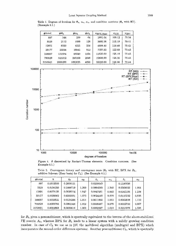
Table 1. Degrees of freedom for Oh, Uh, O'h, and condition numbers (Oh with RT). (Example 6.1.)

1009

# t o t a l #Oh #Uh #O'h /~BPX,Haar

897 544 289 64

3329 2112 1089 128

12801 8320 4225 256

50177 33024 16641 512

198657 131584 66049 1024

790529 525312 263169 2048

3153921 2099200 1050625 4096

~MG ~INV

1991.64 100.12 70.34

3685.58 115.18 70.41

4998.40 119.89 70.42

7597.93 122.68 70.43

11620.00 125.18 70.43

15830.00 126.35 70.43

22030.00 126.86 70.44

10000

1000

100

' ' ' ' ' . , , ~ T " M G ' I R T ( B P X ) - - - x - - -

R T ( B P X . H a a r ) - - - ~ - - - R T ( I N V ) ...... e ......

. - - . . . . . 4~

. . ~h(( . . . . . . . . . . . - oo

. . . . -_.: _~='_'_" L i . . . . . . . . . . x . . . . . . . . . . . . . . . * . . . . . . . . . . . . . . . x

- . ..--"

I I I I I

"El . . . . . . . . . . . . . . . . . . . . . . . . . . . . . . . . . . ~ . . . . . . . . . . . . . . . . . . . . . . . . . . . . . . . . . . ,E l . . . . . . . . . . . . . . . . . . . . . . . . . . . . . . . . . . . ~ . . . . . . . . . . . . . . . . . . . . . . . . . . . . . . . . . . . . E3 . . . . . . . . . . . . . . . . . . . . . . . . . . . . . . . . . . . . E } . . . . . . . . . . . . . . . . . . . . . . . . . . . . . . . . . . . . [ ]

10 I , i ~ i , i t I i i r I

1000 10000 100000 1 e+06

d e g r e e s o f f r e e d o m

Figure 4. 8 discretized by Raviart-Thomas elements. Condition numbers. (See Example 6.1.)

Table 2. Convergence history and convergence rates (Oh with RT, BPX for Bh, additive Schwarz (Haar basis) for Ch). (See Example 6.1.)

h 4

0.0312500 0.2608121

0.0156250 0.1088719

0.0078125 0.0526774

0.0039062 0.0250551

0.0019531 0.0124296

0.0009766 0.0061348

0.0004883 0.0030616

so 5u ~u 5a ~

0.0239543 0.1190020

1.260 0.0094593 1.340 0.0569033 1.064

1.047 0.0047551 0.992 0.0241195 1.238

1.072 0.0024140 0.978 0.0135222 0.835

1.011 0.0011803 1.032 0.0062648 1.110

1.019 0.0005987 0.979 0.0032733 0.937

1.003 0.0002967 1.013 0.0015978 1.035

~ to ta l

897

3329

12801

50177

198657

790529

3153921

for B h gives a p r e c o n d i t i o n e r , w h i c h is s p e c t r a l l y e q u i v a l e n t t o t h e i nve r se of t h e a b o v e - s t a b i l i z e d

F E m a t r i x Ah, w h e r e a s B P X for Bh l eads to a l i n e a r s y s t e m w i t h a m i l d l y g r o w i n g c o n d i t i o n

n u m b e r . I n case of Ch we use as in [33] t h e m u l t i l e v e l a l g o r i t h m ( m u l t i g r i d a n d B P X ) w h i c h

i n c o r p o r a t e s t h e s e c o n d - o r d e r d i f fe rence o p e r a t o r . A n o t h e r p r e c o n d i t i o n e r Ch, w h i c h is s p e c t r a l l y

1 0 1 0 M . M A I $ C H A K A N D E . P . S T E P H A N

10

0.1

0.01

0.001

0.0001

110

100

90

80

J~

E 70 - 1 ¢ -

= 6 0

50

40

30

20

I ' I ' I ' ' I

Potential u (MG) - - + - - Potent ial u (BPX) - - - x - - - Potent ia l u ( INV) - - -~--- F lux The ta (MG) ...... ~ ......

F lux Theta (BPX) - . -= - - . F lux The ta ( INV) - . -e - . -

S igma (MG) . . . . . . Sigma (BPX) --- -~ ---

I i , , I i i , I i , i I

1000 10000 100000 I e+06 degrees of freedom

I • I • I • • i

.xMultigrid i . . . . . x- . . . . . . . . . . . . . . . . BPX - - - x - - -

. . . . . . . . . . × . . . . . . . . . . . . Block- Inverse ---~--- .X - . . . . . . . . . . . . . . . X . . . . . . .

J ..____.+------- ~ J

. . . . . . . . . . . . . . . . . . ~ . . . . . . . . . . . . . . . . . . ~ . . . . . . . . . . . . . . . . . . . ~¢~ . . . . . . . . . . . . . . . . . . ~ . . . . . . . . . . . . . . . . . . .

1000 10000 100000 1 e+06 degrees of freedom

Figure 5. e discretized by piecewise constants. Errors and iteration numbers. (See Example 6.2.)

equivalent to the inverse of the single layer potent ia l ma t r ix Vh up to t e rms depending logari th- mical ly on h, is given by using addi t ive Schwarz me thod based on the Haar basis [34,35]. For Eh in ma t r i x form we choose the ma t r ix h-2I in case of piecewise cons tant basis functions and continuous piecewise l inear basis functions and the ident i ty m a t r i x I in case of R a v i a r t - T h o m a s

Least Squares Coupling Method 1011

r 0

~F C4 - J

.{.=

i3 0

10

0.1

0.01

0.001

0.0001

' ' . . . . . . . ' . . . . . . . . Potential u (M(3) ' - -~-+~ ' Potential u (BPX) - - -x - - - Potential u (INV) ---4--- Flux Theta (MG) . . . . . . { ~ . . . . . .

Flux Theta (BPX) - . -u - - - .~:.. , Flux Theta (INV) -.-e---

:5:~..5~ Sigma (MG) .... ,--- "'"-.~r-~.~--~i * Sigma (BPX) .... ~---

: ~:t::~::~::~ ::~,r ,... ~ . . . . . . . . . . ~- - , - . . . . . . . .

.... -?'-::t.:t:.~.,., . . . . . . . . 8

I l l , i . . . . . . I i , , . . . . . I , , , , , , ,

1000 10000 100000 1 e+06

degrees of freedom

150

140

130

120

110 o

=E c 100

90

80

70

/-

z/"

. J

i -

X j

. . . . . . : M'ultig'rid' ' , ' ' ' ....................... ~3FX- ~=-x--~

Block-inverse ---a---

. . . . . . . . . . . . . . . . . . . . . . - . ~ o . . . 60 ~ : . . . . . . . . . . . . . . . . . . . . . . . . . . . . . . . . . . ~ _

50 ,I , , , , , , , ,I , , , , , , , ,I , , ,

1000 10000 100000

degrees of freedom

Figure 6. O discretized by continuous piecewise linears. Errors and iteration numbers. (See Example 6.2.)

, , t 1

1 e+06

elements. As linear system solver we take the preconditioned conjugate gradient algorithm until

the relative change of the i terated solution is less t han 5 = 10 - s .

Example 6.1 is chosen such that u and a are vanishing on the interface and the jumps u0, to are

zero. In Example 6.2, u and a are nontr ivial on the boundary, bu t the jumps u0, to are vanishing.

In Example 6.3 the jumps u0, to are given explicitly such tha t the solution has a singularity.

1012 M. MAISCHAK AND E. P. STEPHAN

E O ,¢

O J _ J

G )

10

0.1

0.01

0.001

0.0001 I , r , I , , , I , , , I

1000 10000 100000 1 e+06

degrees of freedom

Potential u (MG) , Potential u (BPX) - - -x- - - Potential u (INV) ---~--- Flux Theta (MG) ...... ~ ......

Flux Theta (BPX) - - ~ - - . Flux Theta (INV) -.-e-.-

Sigma (MG) .... .--- Sigma (BPX) .... ~---

160

140

120

1 O0

80

60

40

20

. . . . . . *-" BPX- - -× - - - ._~ . . . . . . . . . . Block-Inverse---~---

. f /

/ - /

/ - /

. . - - +

/

. . . . . . . . . . - )~ . . . . . . . . . . . . . . . . . . . ~ . . . . . . . . . . . . . . . . . . -,v,v,v,v,v,v,v,v, vi~ . . . . . . . .

l , , , I , , i I , I i I

1000 10000 100000 1 e+06 degrees of freedom

Figure 7. 0 discretized by RT-elements. Errors and iteration numbers. (See Exam- ple 6.2.)

Our numerical results (Table 1 and Figure 4 for Example 6.1, F igure 8 for Example 6.3) show

bounded condi t ion numbers for the precondi t ioned sys tem when mul t igr id or the block-inverse are used for Bh and Ch. This is in accordance wi th Theorem 5.1. We also note t ha t the errors

do not depend considerably on the precondi t ioners involved. Only the condi t ion numbers and

Least Squares Coupling Method 1013

iteration numbers are depending on the choice of the preconditioners. For the L 2 errors we write

5a =: 118 - Ohll[L2(a)l:, 5~ = I[u -- UhI[L2(n), and 5~ = I]a - ahHL2(r). In Example 6.1 (Table 1, Figures 1-3) and in Example 6.2 (Figures 5-7) the solution is smooth

and therefore all convergence rates are approaching one. For the solution in Example 6.3 we have u E Hl+2 /3 -e (~ ) , z > 0 arbitrary. Therefore we obtain the theoretical convergence rate with respect to the norm ]](-,., ')]Ix, which is h 2/3-~. The error 6~ is with respect to the L2-norm, whereas the a priori estimate is given in terms of the / t -1 /2 (F) -norm, and therefore we are

losing half an order of convergence rate. Therefore our numerical results correspond to the a

priori estimate in Theorem 4.3. The implementat ion of the least squares coupling method uses only components which are

also necessary in the implementation of the s tandard symmetric coupling method and offers the advantage tha t there is no need for a generalized Krylov method like MINRES or GMRES as

in the case of the symmetr ic coupling method [31,36]. The well-known preconditioned conjugate gradient algorithm is sufficient. The computat ion of the flux is done with negligible implemen- rational effort, because no preconditioner is needed, cf. Theorem 5.1 and the Galerkin matrices involved are sparse and very easy to implement. The numerical experiments presented in this paper are done with the software package maiprogs [37], implemented by one of the authors.

EXAMPLE 6.1. Let ~ = [-0.25,0.25] 2. Let the cut-off function )~ be given by

0, if Ixl _> 3,

i ( x ) ---- 1, if Ix I < 1,

(cos((Ix ] -- 1)(~r/2)) + 1) else. 2

Then we fix f and set u0 = to = 0, a -- 1 such tha t the solution of the transmission prob- lem (1)-(5) is given by ul (x ,y ) : -= )~(12x):~(12y) and u2 --- 0.

In Figure 1 we present the L~-errors and iteration numbers, when the flux 0 is discretized by piecewise constant functions. Figure 2 presents the L2-errors and iteration numbers, when the :flux t? is discretized by continuous piecewise linear functions. Figure 3 gives the L2-errors

and iteration numbers, when the flux 8 is discretized by Raviar t -Thomas elements. For this discretization we show in Table 1 and in Figure 4 the condition numbers, whereas in Table 2 the L~-errors and convergence rates are given.

EXAMPLE 6.2. Let gt = [-0.25,0.25] 2 with X2(x,y) := 1 - )~(12x)~(12y) . The solution of this example is given by u(x , y ) := X 2 ( x , y ) x / ( x 2 + y2), i.e., u0 = to = 0 and u is harmonic outside of ~t, due to x / ( x 2 + y2) = ~(1 /z) .

L2-errors and iteration numbers are presented in Figure 5 when the flux 0 is discretized by piecewise constant functions, in Figure 6 when the flux 8 is discretized by continuous piecewise lineax functions, and in Figure 7 when the flux 0 is discretized by Raviar t -Thomas elements.

Table 3. multigrid preconditioner). (See Example 6.3.)

L2-errors 50, 5~, 5a for Oh, uu, ah and convergence rates (Oh with RT,

~total h 60

0.05517 0.03535 0.02249 0.01425 0.00901 0.00569 0.00359 0.00226

~8 5u 0.0008359

0.642 0.0002838 0.653 0.9398E-04 0.658 0.3147E-04 0.661 0.1203E-04 0.663 0.6128E-05 0.665 0.3801E-05 0.665 0.2468E-05

209 0.06250 705 0.03125

2561 0.01562 9729 0.00781

37889 0.00390 149505 0.00195 593921 0.00097

2367489 0.00048

au 5a aa

0.45692 1.558 0.40826 0.162 1.594 0.36480 0.162 1.578 0.32598 0.162 1.387 0.29128 0.162 0.973 0.26026 0.162 0.689 0.23248 0.163 0.623 0.20758 0.163

0.1

0.01

0.0001

e 0 ,=

" 0.001

l e -05

l e - 0 6 I , , ~ I , , I ,

1000 10000 1 e+06

t - ,

E= t -

O

" ID t -

O

o

I • i i • ' I

Potential u (MG) i . . . . . . . . . . . . . . . . .~ . . . . . . . ~ . Potent ial u (BPX) - - - x - - -

. . . . . . . . . . . . . . . . . . . . . . . . . . . . . 4 . . . . . . . . . . . . . . . . . . . - i . . . . . . . . . . . . . Pot.e•tial u ( INV} ---~---

Flux Theta (BPX) -.-m--- F lux Theta ( INV) ---e---

S igma (MG) .... o--- . . . . ~" - - - - l~ .~_ S igma (BPX) .... ~---

. . . . ~ ~ . t p ,~ .~ .~ ~

1014 M. MAISCHAK AND E. P. STEPHAN i

10000 ,

1000

100

, , I

100000

degrees of f reedom

I:IT ' (MG) I RT (BPX) - - -x - - - RT (INV) " ' -~- ' -

. . . . . . . X . . . . . . . . . . . . . . . . ~ - . . . . . . . . . . . . . . . X . . . . . . . . . . . . . . . -X - . . . . . . . . . . . . . . . X

. . . . . . . . . . . . . . • . . . . . . . . . . . . . . . . . - 2 ( . . . . . . . . . . . . . . . . . . - ~ . . . . . . . . . . . . . . . . . . • . . . . . . . . . . . . . . . . . . ) ~ . . . . . . . . . . . . . . . . . .

10 I , , I , , I , I

1000 10000 100000 1 e+06

degrees of f reedom

Figure 8. Errors and condition numbers, O h with Raviart-Thomas elements. (See Example 6.3.)

EXAMPLE 6.3. Le t £Z be the L - s h a p e d d o m a i n w i t h ver t ices (0, 0), (0, 1 /4) , ( - 1 / 4 , 1 /4) , ( - 1 / 4 , - 1 / 4 ) , ( 1 / 4 , - 1 / 4 ) , and (1 /4 ,0 ) . Now we p re sc r ibe j u m p s w i th s ingu la r i t i e s on the in te r face

F = OgZ and t ake f = 0 in £ / a n d a = 1. Se t t i ng

u0 ( r , ¢) := r 2 /3 sin (27r - ~) - log x - + y - ~ , t0(r , ¢) : = O n '

Least Squares Coupling Method 1015

the solution of (1)-(5) is given by

u l ( r , ~ ) = r2/asin -~(2~r- ~ , in a l ,

u2(r,~)=log~(x-8)2+(y-1) 2, in~2.

T h e e x p e r i m e n t a l convergence ra tes g iven in Table 3 conf i rm the t h e o r e t i c a l convergence rates .

In F i g u r e 8 t h e cond i t i on n u m b e r s for t he p recond i t i oned s y s t e m (42) are p l o t t e d showing excel lent

behav io r for t h e b lock- inverse and t h e mu l t i g r id p recond i t ioner , whe rea s B P X slowly degenera tes .

R E F E R E N C E S

1. M. Costabel and E.P. Stephan, Coupling of finite and boundary element methods for an elastoplastic interface problem, SIAM Y. Numer. Anal. 27, 1212-1226, (1990).

2. M. Costabel and E.P. Stephan, Coupling of finite elements and boundary elements for inhomogeneous trans- mission problems in ~3, In M A F E L A P IV, (Edited by J. Whiteman), pp. 280-296, Academic Press, London, (1988).

3. E.P. Stephan, Coupling of finite elements and boundary elements for some nonlinear interface problems, Comp. Meth. Appl. Mech. Engrg. 101, 61-72, (1992).

4. G. Gatica and G. Hsiao, Boundary-Field Equation Methods for a Class of Nonlinear Problems, Pitman Research Notes in Mathematics Series, 331, (1995).

5. C. Carstensen, E.P. Stephan and D. Zarrabi, On the h-adaptive coupling of fe and be for viscoplastic and elasto-plastic interface problems, Y. Comp. Appl. Math. 75, 345-363, (1996).

6. O.C. Zienkiewicz, D.W. Kelly and P. Bettess, Marriage ~ la mode--The best of both worlds (finite elements and boundary integrals), In Energy Methods in Finite Element Analysis, (Edited by R. Glowinski, E.Y. Rodin and O.Z. Zienkiewicz), pp. 81-107, J. Wiley, (1979).

7. C.N. Gatica, L.F. Catica and E.P. Stephan, A FEM-DtN formulation for a nonlinear exterior problem in incompressible elasticity, Math. Meth. Appl. Sei. 26, 151-170, (2003).

8. U. Brink, C. Carstensen and E. Stein, Symmetric coupling of boundary elements and Raviart-Thomas type mixed finite elements in elastostatics, Numerisehe Mathematik 75, 153-174, (1996).

9. G.N. Gatica, N. Heuer and E.P. Stephan, An implicit-explicit residual error estimator for the coupling of dual-mixed finite elements and boundary elements in elastostatics, Math. Meth. Appl. Sci. 24, 179-191, (2001).

10. P. Boehev and M.D. Gunzburger, Finite element methods of least-squares type, S I A M Rev. 40, 789-837, (1998).

11. J.H. Bramble and A.H. Schatz, Least squares methods for 2m th order elliptic boundary-value problems, Math. Comp. 25, t-32, (1971).

12. E.P. Stephan and W.L. Wendland, Remarks to Galerkin and least squares methods with finite elements for general elliptic problems, Manuscripta Geodaetiea 1, 93-123, (1976).

13. W.L. Wendland, Elliptic Systems in the Plane, Monographs and Studies in Mathematics, 3, Pitman (Ad- vanced Publishing Program), Boston, (1979).

14. D.C. Jespersen, A least-square decomposition method for solving elliptic systems, Math. Comp. 31,873-880, (1977).

15. A.K. Aziz, R.B. Kellog and A.B. Stephens, Least-squares methods for elliptic systems, Math. Comp. 44, 53-70, (1985).

16. G.J. Fix and G.D. Cunzburger, On least squares approximation to indefinite problems of the mixed type, Intl. Journal for Numer. Mtd. in Eng. 12, 453-470, (1978).

17. G.J. Fix, M.D. Gunzburger and R.A. Nicolaides, Least squares finite element methods, Math. and Comp. with Appls. 5, 87-98, (1979).

18. G.J. Fix and E.P. Stephan, On the finite element-least squares approximation to higher order elliptic systems, Arch. Rational Mech. Anal. 91, 137-151, (1985).

19. J. Bramble, R. Lazarov and J. Pasciak, A least-squares approach based on a discrete minus one inner product for first order systems, Math. Comp. 66, 935-955, (1997).

20. G. Gatica, H. Harbrecht and R. Schneider, Least squares methods for the coupling of fem and bem, SIAM J. Numer. Anal. 41 (5), 1974-1995, (2003).

21. J. Bramble, J. Pasciak and J. Xu, Parallel multilevel preconditioners, Math. Comp. 55, 1-22, (1990). 22. V. Girault and P.-A. Raviart, Finite Element Methods for Navier-Stokes Equations. Theory and Algorithms,

Springer-Verlag, (1986). 23. M. Costabel, Boundary integral operators on Lipschitz domains: Elementary results, S I A M J. Math. Anal.

19 (3), 613-626, (1988). 24. I. Sloan and A. Spence, The Galerkin method for integral equations of the first kind with logarithmic kernels:

Theory, []VIA J. Numer. Anal. 8, 105-122, (1988).

1016 M. MAISCHAK AND E. P. STEPHAN

25. E.P. Stephan and W.L. Wendland, An augmented Galerkin procedure for the boundary integral method applied to two-dimensional screen and crack problems, Applicable Anal. 18, 183-219, (1984).

26. C. Carstensen and E.P. Stephan, Adaptive coupling of boundary and finite element methods, Math. Modelling Num. Analysis 29, 779-817, (1995).

27. P.G. Ciarlet, Basic error estimates for elliptic problems, In Handbook of Numerical Analysis Volume II, (Edited by P.G. Ciarlet and J.L. Lions), pp. 17-352, North-Holland, Amsterdam, (1991).

28. J.E. Roberts and J.M. Thomas, Mixed and hybrid methods, In Handbook of Numerical Analysis Volume II, (Edited by P.G. Ciarlet and J.L. Lions), pp. 523-639, North-Holland, Amsterdam, (1991).

29. G. Strang, Variational crimes in the finite element method, In The Mathematical Foundations of the Finite Element Method with Applications to Partial Differential Equations, (Edited by A. Aziz), pp. 689-710, Academic Press, New York, (1972).

30. G. Strang and G.J. Fix, An Analysis of the Finite Element Method, Series in Automatic Computation, Prentice-Hall, (1973).

31. S.A. Funken and E.P. Stephan, Fast solvers with multigrid preconditioners for linear fem-bem coupling, Preprint, University of Hannover, (2001).

32. N. Heuer, M. Maischak and E.P. Stephan, Preconditioned minimum residual iteration for the h-p version of the coupled fem-bem with quasiuniform meshes, Numer. Linear. Algebra. Appl. 6, 435-456, (1999).

33. J. Bramble, Z. Leyk and J. Pasciak, The analysis of multigrid algorithms for pseudo-differential operators of order minus one, Math. Comp. 63, 461-478, (1994).

34. T. Tran and E.P. Stephan, Additive Schwarz method for the h-version boundary element method, Applicable Analysis 60, 63-84, (1996).

35. M. Maischak, E.P. Stephan and T. Tran, Domain decomposition for integral equations of the first kind: Numerical results, Appl. Anal. 63, 111-132, (1997).

36. P. Mund and E.P. Stephan, The preconditioned GMRES method for systems of coupled fem-bem equations, Advances in Computational Math. 9, 131-144, (1998).

37. M. Maischak, Manual of the software package maiprogs, Technical Report ifam48, f t p : / / f t p . i ~ a m / u n i - hannover , d e / p u b / p r e p r i n t s / i f a m 4 8 , ps . Z, Institut fiir Angewandte Mathematik, Universitiit Hannover, (2001).