A weighted least squares method for first-order hyperbolic systems

INTERNATIONAL JOURNAL FOR NUMERICAL METHODS IN FLUIDS, VOL. 20, 191-212 (1995)

A WEIGHTED LEAST SQUARES METHOD FOR FIRST-ORDER HYPERBOLIC SYSTEMS

D. G. ZEITOUN*, J. P. LAIBLE AND G. F. PINDER College of Engineering and Mathematics, IOI btey Building# Universiv of Vermont, Burlington, VT 05403, US.A.

SUMMARY

The paper presents a generalization of the classical L2-norm weighted least squares method for the numerical solution of a first-order h erbolic system. This alternative least squares method consists of the minimization of the weighted sum of the L residuals for each equation of the system. The order of accuracy of global conservation of each equation of the system is shown to be inversely proportional to the weight associated with the equation. The optimal relative weights between the equations are then determined in order to satisfy global conservation of the energy of the physical system.

As an application of the algorithm, the shallow water equations on an irregular domain are first discretized in time and then solved using Laplace modification and the proposed least squares method.

Y P .

KEY WORDS Weighted least squares Hyperbolic system of equations Shallow water equations Newton-Raphson method

1. INTRODUCTION While there are a number of different least squares formulations for solving boundary value problems, they may be generally classified into three groups.

In the first group the partial differential equation is transformed into an optimal control problem via the introduction of a state function, the solution of a given state equation. This equation is generally discretized using a Galerkin finite element approximation. The least squares solution algorithm employs a conjugate gradient method. Conservation of mass and satisfaction of boundary conditions are assured by requiring the state vector to belong to a suitable Sobolev space.','

In the second group the least squares approximation is combined with the Galerkin finite element method to obtain convergent finite element approximations. An example of this type of method is the Galerkin least squares method developed by Hughes et al.3 In this approach the least squares form of the residual is added to the Galerkin method in order to stabilize the Galerkin method without degrading accuracy.

In the third group the mathematical form of the approximate solution (trial solution) is first chosen and then the norm of the corresponding residual is minimized by least s q ~ a r e s . ~ This is the approach addressed in the present paper.

A collocation L2 least squares formulation is proposed herein which takes into account in an optimal way the relative weights identified with the different equations of the system. While the methodology developed in this paper may be applied to various types of partial differential equations, herein the solution of a first-order hyperbolic system generally denoted as the shallow water equations is considered.

*Present address: TAHAL Consulting Eng. Ltd., PO. Box 1 1 1700-61 11, Tel-Aviv, Israel.

CCC 027 1-2091/95/030191-22 0 1995 by John Wiley & Sons, Ltd.

Received 13 December 1993 Revised 19 May 1994

192 D. C. ZEITOUN, J. I? LAIBLE AND G . E PMDER

After a brief review in Section 2 of numerical methods for solving first- order systems of partial differential equations, basic definitions and mathematical properties of the weighted least squares method are discussed in Sections 3 and 4. The absence of global conservation properties of the classical least squares formulation leads to a new method proposed in Section 5 and applied to the solution of the shallow water equations in Section 6.

2. NUMERICAL METHODS FOR FIRST-ORDER SYSTEMS

Let R be a bounded domain in the (x, y ) plane with boundary r. The vector n = ( n x , ny) is the outward unit normal to r. The first-order system of coupled equations considered in this work may be written as

au a u LU A- + D- + CU = f ,

ax ay

with the boundary condition

BU (An, + Dny - M)u = g.

A, D, C and M are p x p matrix-valued functions, the column vector forcing term is fT = c f i , f i , . . . , f , ) , gT = (g,, g2, . . . , gpb) is the column vector of applied boundary conditions and the unknown column vector is uT = (u , , u2, . . . , up) ( T denotes transposition). L represents the linear differential operator defined in the domain R and B represents the boundary differential operator.

Sufficient conditions for problem (l), ( 2 ) to have a unique strong solution have been obtained for symmetric positive systems in the sense of Friedrichs.’

Numerical approximations of pure hyberbolic problems have been extensively studied. Different schemes based on finite difference and Galerkin finite element approximations have been proposed for the solution of linear and non-linear hyperbolic equations and first-order systems (see Reference 6 for a review).

A perceived disadvantage of the least squares method compared with the Galerkin method is the higher-order finite element continuity requirement. However, for basis hnctions defined on rectangular subspaces, such as in the case presented herein, these continuity conditions are easily accommodated and higher-order accuracy and function continuity are achieved. These higher-order continuity constraints may be circumvented by expressing higher-order equations as sets of lower- order equations, although additional field variables are thereby introduced.

The standard Galerkin method leads to ‘central-type’ discrete operators which exhibit oscillatory behaviour on practical meshes. A way to avoid this difficulty is to select a test function for the convective term that explicitly accommodates the directional property of the hyperbolic propagation (upwinding). Such methods are often denoted as Petrov-Galerkin methods. The main drawback of this approach is the absence of a generally applicable systematic procedure for the selection of the test function. Recently the Lax-Wendroff scheme has been used for developing the Taylor-Galerkin method. In addition, the method of characteristics has been used for developing the Galerkin method.

Finite element methods for solving first-order systems which are symmetric and positive in the sense of Friedrichs have been proposed by Lesaint and R a ~ i a r t . ~ For symmetric systems arising out of the heat equation, Aziz and Liu8 proposed a weighted least squares solution method. In their work a unique weight associated with the boundary conditions was determined in order to reduce the error estimates.

For mixed methods based on splines, the least squares theory for second-order elliptic systems developed in Reference 9 specifies the optimal weights in terms of the spline mesh size. Other first- order systems have also been solved numerically using a weighted least squares formulation where

FIRST-ORDER HYPERBOLIC SYSTEMS 193

optimal weights are found theoretically. For example, Wendland" formulates a least squares method for strong elliptic systems satisfying the Lopatinsky conditions for the boundary operator. For elliptic operators in the sense of Douglis and Nirenberg, wherein the operator satisfies the supplementary condition for the operator L and the complementary conditions for the boundary operator B, a weighted least squares method has been proposed by Aziz et al."

A difficulty appearing in the implementation of the method, and one that is addressed in this paper, is the determination of the weights associated with the least squares method for a general first-order system. In most numerical implementations these weights must be specified by the ana ly~t .~ Without some rational criteria for selecting these weights, the efficiency of the method may be seriously affected even if other computational objectives are achieved.

The formulation proposed herein is similar to the least squares finite element method proposed by Jiang and Carey for linear and non-linear hyperbolic system^.'^-'^ However, the method differs in as much as collocation points and weighting functions are introduced.

As noted earlier, the least squares method is validated on the two-dimensional shallow water equations. These equations are oilen used to obtain flow fields necessary for pollution problems and transport in shallow estuaries. A special advantage of using the collocation least squares method for solving the shallow water equations is the ability to solve the equations in an irregular domain with a completely orthogonal computational mesh. l 5 , l 6 This significantly enhances both the accuracy and computation time.

When the non-linear terms appearing in these equations are linearized, they reduce to a system of first-order equations. Classical collocation least squares has good noise control characteristics compared with the Galerkin method when solving the shallow water equations. However, one of the difficulties inhibiting its widespread use is that the accuracy of the solution depends upon the weights appearing in the formu1ation.l6

3. A WEIGHTED LEAST SQUARES METHOD

A least squares formulation is proposed herein which takes into account the relative weights between the different first-order equations appearing in the system. The least squares formulation is presented in terms of the matrix of differential operators L and B defined in equations (1) and (2). These equations may be written as

Lu = f in R, B u = g on r. (3) In order to formulate the method proposed, let us now define the functional spaces and their

associated norms. In the following we define the working space Vg as the p-product of the Sobolev space H'(Q):

V, =H'(R) x H y Q ) x " ' x H ' ( Q ) = [H'(R)]P, \ d

Y

p times

I H'(R) = { v E P ( Q ) ; - E 2(Q);- E L*(Q) 8 V d V

d X 8Y

(4)

Notice that each element u E Vg is a vector of p components ui, i = 1, 2, . . . , p.

may be defined on the domain 0 and the boundary r as If for any u E V, and v E V,, u . v denotes the classical scalar product on Rp, an L2 scalar product

(u, v) = IQ u . vdQ, [u, v] = Ir u . vdr. ( 5 )

194 D. G. ZEITOUN, J. P. LAIBLE AND G. F. PINDER

In the following, 11 . Iln denotes the norm associated with (., .) and 1 1 . Ilr denotes the norm associated with [., .I.

The L2 weighted least squares formulation proposed in this work may be separated into two groups.

Group 1. L2 continuous least squares

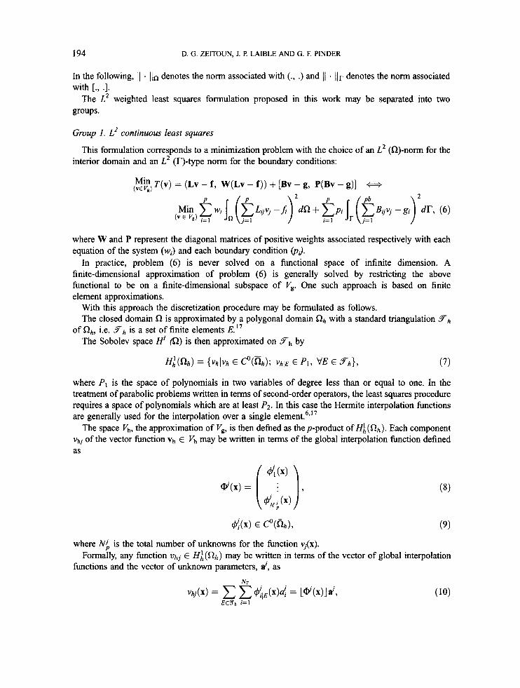
interior domain and an L2 (T)-type norm for the boundary conditions: This formulation corresponds to a minimization problem with the choice of an L2 (R)-norm for the

Min T(v) = (Lv - f , W(LV - f ) ) + [Bv - g, P(Bv - g)] (V€ V&?)

1

where W and P represent the diagonal matrices of positive weights associated respectively with each equation of the system (w;) and each boundary condition (pi).

In practice, problem (6) is never solved on a functional space of infinite dimension. A finite-dimensional approximation of problem (6) is generally solved by restricting the above functional to be on a finite-dimensional subspace of V.. One such approach is based on finite element approximations.

With this approach the discretization procedure may be formulated as follows. The closed domain R is approximated by a polygonal domain R h with a standard triangulation Fh

The Sobolev space H' (32) is then approximated on y h by of Oh, i.e. Fh is a set of finite elements E."

H;(Rh) = {VhIVh E c"(%); VhiE E p1, E Y h } , (7)

where P I is the space of polynomials in two variables of degree less than or equal to one. In the treatment of parabolic problems written in terms of second-order operators, the least squares procedure requires a space of polynomials which are at least P2. In this case the Hermite interpolation functions are generally used for the interpolation over a single element.6"7

The space vh , the approximation of Vg, is then defned as thep-product of H i ( s 2 h ) . Each component vhj of the vector function v h E Vh may be written in terms of the global interpolation hnction defined as

4b) E c " ( f i h ) , (9)

where N i is the total number of unknowns for the function vJ{x).

functions and the vector of unknown parameters, a', as Formally, any function vhj E Hi(Rh) may be written in terms of the vector of global interpolation

NT


where NT is the number of unknowns on the element E. The independent space variable of the domain is represented by x. The L2 approximate continuous least squares formulation consists of the minimization of a functional Zc(a, W, P) containing a weighted sum of the interior and boundary residuals with respect to the unknown vectors a'.

The interior residual RLi corresponding to the ith equation of the system and the boundary residuals RBi corresponding to the ith boundary condition are defined by

Consider now the global unknown vector a formed by the set of all the vectors a', j = 1, . . . , p . The objective fimction Zc(a, W, P) to minimize may be defined as

The approximate L2 continuous least squares formulation corresponding to equation (6) may be defined as

In this general framework an error analysis of the least squares approximation has been conducted for particular problems in fluid dynamic^.',^,^,'^ The choice of a suitable norm 1 1 . on Vg depends on the type of differential operator. For example, the choice of an H1-norm instead of the classical L2-norm stabilized the least squares solution of non-linear hyperbolic problems which generate shock^.'^

Group 2. L2 collocation (or discrete) least squares

The discrete formulation corresponding to the continuous least squares method, also called collocation least squares, consists of selecting a series of collocation points inside the domain and on the boundary and minimizing the hnction

The points x I for 1 = 1, . . . , k correspond to the interior points and for 1 = k+ 1, . . . , m to the boundary points of 0.4 The weights q are associated with the collocation points. One of the difficulties appearing in the implementation of the method is the determination of the weights wi, i = 1, . . . , p, the weights p i , i = 1, . . . , p , and the weights q, 1 = 1, . . . , m.

The addition of the integral of the boundary residual may result in a solution vector with large interior residuals. This scaling problem may degrade the satisfaction of the governing balance laws. This is particularly true when the weights appearing in the matrix P are very large.

196 D. G . ZEITOUN, J. P. LAIBLE AND G. F. PMDER

Basically, the three types of weights introduced (wi, pi and q) are each of a different nature. The first and second types of weights, wi, i = 1, . . . , p , and p i , i = 1, .. . , p b . determine the relative contributions of the interior and boundary residuals. When a system of equations is solved using an L2 least squares method, these weights will balance the different contributions of each equation and each boundary condition. These weights are generally specified by the analyst.

The third type of weights, cI. i = 1, . . . , m, represent the distribution of weights among the collocation points. These weights may be determined by using optimal criteria for numerical integration, such as Gaussian quadrature. For a collocation least squares method using finite element discretization, the use of Gaussian points and their weights leads to an optimal truncation error. More sophisticated criteria have been proposed by the authors.’’

In the present work we concentrate on the first and second types of weights and a general methodology is developed for computation of the optimal values of these weights.

4. PROPERTIES OF THE L2 LEAST SQUARES

In the least squares literature two different methods have been proposed for computing the numerical solution of the minimization problem (problem (1 3) here). The first consists of using an unconstrained optimization algorithm for the quadratic functional I, or Z,. Classical methods such as conjugate gradient or quasi-Newton generally require the computation of both a hnctional and its Jacobian. The second approach consists of solving the normal equation coresponding to a first-order necessary condition for a minimum of the functional.

In the present work we deduce the normal equation from the multidimensional minimization problem (equation (6)) rather than from the finite-dimensional problem as is usually done. Then we discuss the basic properties of the least squares method.

The following theorem gives a necessary condition for a minimum for the least squares and approximate least squares methods.

Theorem 1

If U, resp. uh , is the vector solution of the minimization problem (6), resp. (1 3), then for all v E V,, resp. v h E vh .

(LG - f , ~ ( L v ) ) + [BG - g, P(Bv)] = 0,

(Luh - f , w(Luh)) + [BUh - g, P ( B v ~ ) ] = 0.

(15)

(16)

Proof Consider the least squares functional J(v) = (Lv - f, W(Lv - f)) + [Bv - g,P(Bv - g)]. If U is a solution of equation (1 5) , then Vv E V,

J(U + tv) - J(U) lim 2 0. 1-0 t

The Taylor expansion of J ( U + tv) may be written as

J(U + tv) = J(U) + t{(LG - f , ~ ( L v ) ) + [BG - g, P(Bv)]} + O(t2) .

Then for all v E V, and for t > 0 the above limit leads to

(LG - f , ~ ( L v ) ) + [BG - g, P(Bv)] 2 0.

Taking now -v instead of v in the last inequality, we see that we obtain (15).


The same proof may be developed for the approximate least squares problem (equation (1 6)).

Equation (1 6) may be written as a linear system of algebraic equations with unknown vector a. The solution vector uh and the weighting function vector vh may be expressed in terms of their components as

uhj(x) = [w(x)]d, %j(X) = L@'(x)J&. (19) Equation (16) may be written in terms of the components of the differential operators L and B as

Let us assume that for any j = 1, . . . , p the dimension of the column vector a' is independent of j and equals D. Introduce now the fl x php matrices Y' and the two multipliers LXx) and Bi(x) defined as

With this notation equation (1 6) may be written in matrix form as

where the matrices Ai and Bi and the vectors fi and gi are defined for continuous least squares as

Lf(x)Li(x)dx, B; = bT(x)bi(x)dx, fi = LT(x)fidx, gi = J, bf(x)g;dx

(23) and for collocation least squares as

(24) Equation (22) is valid for any vector d and may therefore be written in the classical form of the normal equation, i.e.

Without loss of generality, equation (25) may be scaled such that the first weights wI will be equal t one. Defining the new weights ei = l/wi, i = 2, . . . , p, and vj = l/wj, j = 1, . . . , Pb, equation (25) may now be expressed as

198 D. G. ZEITOUN, J. F! LAIBLE AND G . F. PMDER

The choice of the optimal relative weightings depends on the criterion of optimality defined. For the numerical least squares method presented in this contribution, these criteria may be separated into four categories:

(a) accuracy of the numerical scheme (b) numerical stability of the linear system resulting from the normal equation (25) (c) satisfaction of the boundary conditions (d) conservation of the mass balance.

The dependence of the weighting on the overall accuracy of the numerical scheme is still a subject of research. Error estimates using different norms on suitable Sobolev spaces have been derived by several authors for the penalty method (see e.g. Reference 9). Compared with our formulation, the classical penalty method corresponds to a system with two equations and a single weight. The optimal weight is chosen for the reduction of the error estimation. This weight depends on the type of partial differential equation, the discretization parameter and the type of boundary conditions. Such analysis shows that a better theoretical error estimate is obtained when the weight is reduced.

It is well known that for a large weight the condition number of the normal equation resulting from the penalty least squares method depends linearly on this weight.' According to this criterion, one has to increase the weight for a good stability of the normal equation.

Thus the weighting strategy for criterion (a) is the opposite of that for criterion (b). Among the basic properties we may require from a numerical method, global conservation of the

system is of primary imp~rtance.~ This property depends on the physical problem to be solved and on the type of differential operator. It may be stated that the flux, the energy or the forces will be conserved globally inside R. For the first-order hyperbolic system considered here, the global conservation property may be written for each equation of the system as follows:

The global conservation property is not always satisfied by the numerical solution of the weighted least squares formulation presented herein. On the basis of Lagrangian multiplier functions, the order of accuracy of the global conservation property is analysed. The following theorem presents an error estimate for the global conservation property for each equation of the first-order system.

Theorem 2

If a is the vector of dimension plv" which is the solution of equation (26), then we have the following.

(i) For the continuous least squares method the following properties hold:

Pb f o r i = 1 ,..., pb, ~ B i j u ~ - g i = D i v i + O ( v ~ ) .

j = 1


(ii) For the collocation least squares method the following properties hold:

Here the function H,(x) does not depend on and Di does not depend on vi

Prooj The proof is developed in the Appendix. 0

For first-order systems a rigorous study of the dependence of the weights on the accuracy of our least squares formulation is outside the scope of this contribution. However, Theorem 2 points out the difficulty in choosing the relative weights appearing in the least squares functional between the different equations.

In terms of global mass balance conservation, the weighting strategy is to increase all the weight appearing in equations (28) and (29). However, in terms of conditioning of the matrix, the weighting strategy is to reduce these weights. For a given equation (i) the choice of a small value for one of the ci, i = 2, . . . , p, will improve the global conservation property for this equation. A good strategy should be to choose large weights for each equation, but unfortunately this will cause ill conditioning in the linear system of equations (26).

So far the goal of Theorem 2 and the above discussion was to justify the need for the definition of a strategy of optimal weighting.

In the following a criterion of optimality based on energy balance considerations is introduced for the computation of these weights.

The optimal weights are those for which the corresponding least squares solution respects more accurately the mechanical energy balance of the system. This balance equation corresponds to the natural proportions between the different equations.

For the first-order hyperbolic system considered here, one may require a conservation property of the type

which may be written in a functional form as

Oa(v) = 0. (31)

The property of global conservation is implicitly verified in the Galerkin method but is not respected by the formulation (6).

The basic idea of the new least squares formulation proposed is to determine the optimal set of weights wi. i = 1, . . . , p, and p i , i = 1, . . . , p, in order that the least squares solution will respect approximately the global Conservation law Ya(v) = 0. In the case where Y a ( v ) is a positive function, the determination of the optimal set of weights may be achieved by minimizing the function Y,(v) with respect to the weights.


5 . OPTIMIZATION ALGORITHM

5.1. General methodology

The basic steps of the methodology proposed are as follows. Consider after k iterations the set of known weights W k and pk.

Step 1. Determine uh(x, Wk, Ps = ArgMin J(v), the solution of the minimization problem (6).

Step 2. For a positive function Ya(v), determine the new matrices with positive coefficients, W(@l) and P(k+l), which are obtained via solution of the minimization problem with respect to the weights:

MinY,(uh, W(k+l), P@+')) (wi > 0; p ; > 0; i = 1, . . . , p ) .

Step 3

If I @ \ E a ( ~ h , W(k+'), P(kf*))l < E then END If not

GO TO Step 1.

In the next section the algorithm developed for the solution of the shallow water equations is

Set Wk = W(k+l) and pk = P(k+lf

presented.

5.2. Methods and procedures

Here we describe the process for determining the weights used in the present least squares method. An associate norm derived from an auxiliary finite element formulation is first computed. Then the weights are determined in order to force the auxiliary norm to a minimum. In the following we will need to distinguish between the discretized form of the differential equations as derived from the least squares method and the discretized form of the differential equations as derived by some other finite element procedure. We will denote the discretized least squares formulation equation (25) as

A x - f = O , (32)

where

P P

A = C ( w i A i +pjBj), x = a, f = C ( w i f i + pigi) 9 (33) i= 1 i= 1

and the discretized auxiliary formulation as

Aaxa - fa = 0.

One possible auxiliary norm may be defined as

(34)

where x(S) represents the least squares solution for a given set of weights S = (s1, s2, . . . , SZ,) = (wl, w2, . . . , w,, p l , . . . , p,) and T denotes the transposed vector. Notice that x(S) is not the solution of the auxiliary formulation. Since A and fare dependent on the weights used in the least squares formulation, x is also a fbnction of the weights. Our minimization probIem may thus be

FIRST-ORDER HYPERBOLIC SYSTEMS 20 I

stated as

Min @,(x(S))subject to A(S)x(S) - f(S) = 0, si > 0. SI C2,... ,SZn

Here we detail a procedure to solve this problem and contrast this approach with the well- known Newton-Raphson and quasi-Newton methods. Consider a first-order Taylor expansion of x(S) around S:

@a = [A,(x + Vsx . (AS)) - fa] . [Aa(x + Vsx . (AS)) - fa] + o(llAS112), (37) where T,x represents the gradient vector of the vector x with respect to the weights (also called the sensitivity matrix). Applying the minimization criterion aYa/aAS = 0 as in a least squares problem, we obtain

[GTAzAaG](AS) = -[GTA:]{Aax - fa},

where G = T,x is the sensitivity matrix. This matrix is obtained by differentiation with respect to each weight si of the least squares equation:

a -[AX - f]. asi Expanding this last equation and solving for dxldsi yields

ax g. ' = - asi = A-'{ - k]~}.

(39)

The sensitivity matrix G is thus defined as G = [g, (g2(g,( - + a lg,,], where n is the number of weights. The steps of the procedure are as follows.

1. Assume a set of weights S. 2. Solve Ax-f= 0. 3. Employ equation (40) to obtain G. 4. Form and solve equation (38) to obtain AS. 5. If IlASll < end; else S"" = So'd+a{AS} and go to step 2.

Alternatively one may expand Ya around the vector So by Taylor's theorem to obtain

@a = @,(So) + Vs(@a) . {AS} AS} . H~{AS} + ~ ( I I A s I ~ ~ ) , (41)

where H, is the Hessian matrix of Ya with respect to the weights and AS = S - So. The minimum of Ya is obtained from aYa/aAS = 0. This yields

Hs{AS} = -Vs(@a) = GTAT[A,x - fa] (42) This last equation is the basis for the second-order Newton-Raphson methods. It can be shown that the exact expression for the second-order derivatives is

where [[aC/aS]] is a third-order tensor. For the problem under consideration this tensor can be determined analytically but not without considerable computational expense. To improve on the inverse of the Hessian matrix, one can employ the BFGS methods readily available in the IMSL Fortran Library.

202 D. G. ZEITOUN. J. P. LAIBLE AND G. F. PINDER

6. HYPERBOLIC SHALLOW WATER EQUATIONS

Here we discuss a specific case of the general methodology defined in Section 4. The specific equations used are the shallow water equations, which may be written in scalar form as

dv & a\, c b - + u-+ v- + -v+fu + g - - 2 = 0, at ax + H + H

i3C ~(Hu) ~ ( H v ) -+- + - - r = o , at a x ay

r - r p = 0,

(45)

(47)

lxu + 1p = V", (48)

H = h + ( . (49) The first two equations are the x- and y-momentum equations respectively. The third equation is the fluid continuity equation. These equations are valid over the region Q. The fourth equation is a prescribed surface elevation to be enforced on a portion 0, of the boundary and the fifth equation is a prescribed normal flow to be applied on a portion (D2 of the boundary. The last equation defines the total depth. For problems with moving boundaries this equation becomes a third-type boundary condition. Here we will restrict our attention to problems of constant geometry. In these equations x and y are Cartesian co-ordinates, t is time, g is gravity, f is the Coriolis parameter, Cb is the bottom friction parameter, u and v are x and y vertically integrated velocities respectively, [ is the surface elevation, h is the water depth from mean sea level, cp is the prescribed surface elevation, v, is the prescribed normal velocity, 1, and l,, are the direction cosines of the outwardly directed unit normal on the boundary, T, and T~ represent the x- and y-components of the wind shear stress respectively and r is the fluid source. The bottom friction parameter may take on various forms and is generally dependent on u and v.

These equations in their full non-linear form have been solved by the least squares method on irregular domains developed by Laible and Pinder." Since we wish to use a test problem that has an analytic solution, we will focus on the linearized form of these equations.

Starting with the scalar equations, we now seek to bring the shallow water equations into the form of equations (1) and (2). First we note that the continuity equations can be expanded in terms of h and t. Inserting the equality H = h + ( into the continuity equation, the following continuity equation may be obtained:

This equation is now in terms of the first-order derivatives of the unknowns u, v and 5. Equations (44H46) are non-linear. We now seek to obtain a linearized form. Here we introduce a

modification (similar to the idea of Laplace modification used to solve problems with time-dependent coefficients). This modification is applied to all the non-linear terms of equations (44)-(46). Suppose we select some time-invariant characteristic values for u, v and h denoted as U, Vand Hi. These values must generally be greater than any anticipated values of u, v and h respectively. The modification is accomplished by writing an identity equation for each of equations (44)-(46) containing the non-linear


terms. To illustrate the process, we will consider equation (44) and deduce the remaining ‘Laplace- modified’ equations. The identity for equation (44) may be written as

The wind stress term r,/H and Cb are taken here to be independent of u, v and C;, although they could also be similarly treated.

If we now subtract this identity from equation (44), one obtains

=(U-u)-+(V-v)-+ all (; --- ;)+$ a x ?Y (53)

This process itself does not introduce any numerical approximations. In the numerical formulation, however, the left-hand side now contains a linear operator with constant coefficients. In the solution process values of u, v and H are assumed known (from a previous time step or by extrapolation from previous values). Therefore the right-hand side will contain known values. After solution for u, v and ( the right-hand side is updated and the system solved again. Iteration within a time step is carried out until some norm of the variation of u, v and 5 meets a convergence tolerance. In the following we will denote the assumed or extrapolated values for u, v and C; on the right-hand side as u*, v* and <* (also H* = h + <*).

Applying this modification to equations (45) and (46), we finally have

(56)

where

au* w t X

ax aiy k” = (U - u*)- + (V - v*)-+ (2 - Z)U* + H’

Fv=

(57)

We now introduce the time discretization scheme. The local time derivative term is approximated by a backward difference, e.g. &/at x (u’ - u - ) / A t . The variables u, v, C;, u*, v+ and <* are evaluated at an intermediate time between t and t + At by the trapezoidal rule, e.g. u = au+ + (1 - a)u-. Here u+ is


at time t + At and u- is at time t. With these approximations we may finally collect all terms that multiply u, du/& and as in the standard form of equation (1). The vector u is now taken as

u = { i}. After some rearrangement we find

al+ al+ A, - + D, - + C,U+ = f ,

d X ay where

A , = [I ,“u 71, D , = a t a:], 0 aU 0 ah aV

c, =

au- aY

+ Dg- + C ~ U -

c b af -+-a At H

0

0

ah a-

8X

The matrices [A]s, [D]b and [C], are identical to [A],, [B], and [C], except that a is replaced by

The boundary conditions are also written in the standard form (equation (2)) as p = (a-1).

0 0 1 [n, ny 01( ;}={;I

Residuals

It is now possible to express the residuals of the differential equations and boundary conditions in terms of the standard matrices [A], [D], [C] and [MI. Here we use the matrix notation dropping the subscript CL. To develop the residuals due to time and space discretization, we now introduce the spatial approximations. We introduce basis hnction expansions of our unknowns with local support over rectangular finite elements:


The vector L4iJ contains the four basic functions for the bilinear rectangular element. The matrix [E] is thus a 3 x 12 matrix and {ii} is a 12 x 1 vector of nodal values on an elemental region.

Substitution of (63) into equation (61) yields the residuals over the domain R,

and over the boundary r,

cr = { :=} = [MI[QI{U}+ - {g}.

Collectively we may write the residuals as

or equivalently

{c} = [LB+]{U}+ - [LB-]{U}- - , (64) {i 1 where {U}+ and {U}- are the vectors of nodal values of the variables at two different time levels and [LB+] and [LB-] are the numerical counterparts of the differential operator matrix [LB].

The total squared weighted residual is given by

E2 = c {c}~[S]{C}. (65) n,r

Substitution of equation (64) into equation (65) and application of the minimization criterion dE2/d{u}+ = 0 leads to

[A]+{u}+ - {F} = 0, (66) where

[A]’ = c [LB+]T[S][LBf], (67) w-

[A]- = e [LB+IT[S][LB-],

6. I . Test problem description

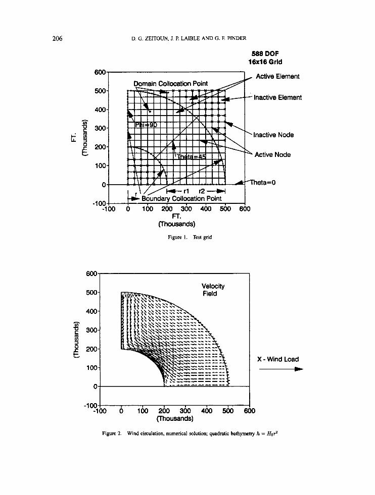
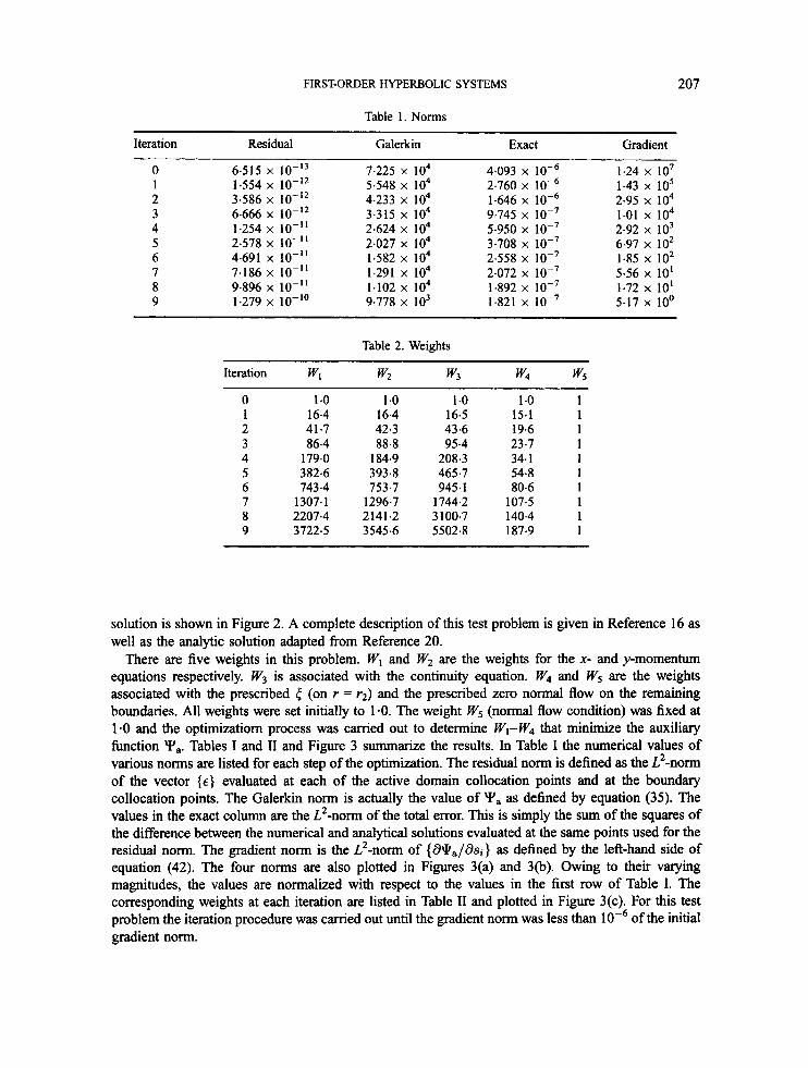
The test problem is shown in Figure 1. The quarter-ring domain has a quadratically varying bathymetry defined by h = H,/ , Ho = hl/rq, hl = 16 m. The surface elevation is prescribed at the outer boundary (r = 2) and all other boundaries have a zero-normal-flow condition. The steady state numerical and analytical solutions were obtained for an x-directed constant wind loading. The velocity

206 D. G . ZEITOUN, J. P. LAIBLE AND G. F. PINDER

588 DOF 16x16 Grid

Active Element

Inactive Element 500

400

300

200

100

0

-1 00 -100 0 100 200 300 400 500 600

FT. (Thousands)

Figure 1. Test grid

500-

400-

2 300- n v)

a 7 g 200-

100-

Velocity

-100 ' 1 I ' -1b0 6 l w 2bO 300 400 500 6 (Thousands)

X - Wind Load ____)

Figure 2. Wind circulation, numerical solution; quadratic bathymeby h = Ho?


Table 1. Norms ~ ~ ~~

Iteration Residual Galerkin Exact Gradient

0 1 2 3 4 5 6 7 8 9

6.515 x 1.554 x lo-'* 3.586 x 6.666 x 1.254 x lo-'' 2.578 x lo-'' 4.691 x lo-" 7.186 x lo-'' 9496 x lo-" 1.279 x lo-''

7.225 x lo4 5.548 x lo4 4.233 x lo4 3.315 x lo4 2.624 x lo4 2.027 x lo4 1.582 x lo4 1.291 x lo4

9.778 x lo3 1.102 x lo4

4.093 x 2.760 x 1.646 x 9.745 x 1 0 - ~ 5.950 x lop7 3.708 x lop7 2.558 x lop7 2.072 x 1.892 x 1.821 x lop7

1.24 x lo7 1.43 lo5 2.95 lo4 1.01 lo4 2.92 x lo3 6.97 x lo2

5.56 x 10' 1.72 x 10' 5.17 x 10'

1.85 x 10'

Table 2. Weights

Iteration Wl w2 w3 w4 WS

0 1 2 3 4 5 6 7 8 9

1 .o 16.4 41.7 86.4

179.0 382.6 7434

1307.1 2207.4 3722.5

1 .o 16.4 42.3 88.8

184.9 393.8 753.7

1296.7 2141.2 3545.6

1 .o 16.5 43.6 95.4

208.3 465.7 945.1

1744.2 3 100.7 5502.8

1 .o 15.1 19.6 23.7 34.1 54.8 80.6

107.5 140.4 187.9

~

1 1 1 1 1 1 1 1 1 1

solution is shown in Figure 2. A complete description of this test problem is given in Reference 16 as well as the analytic solution adapted from Reference 20.

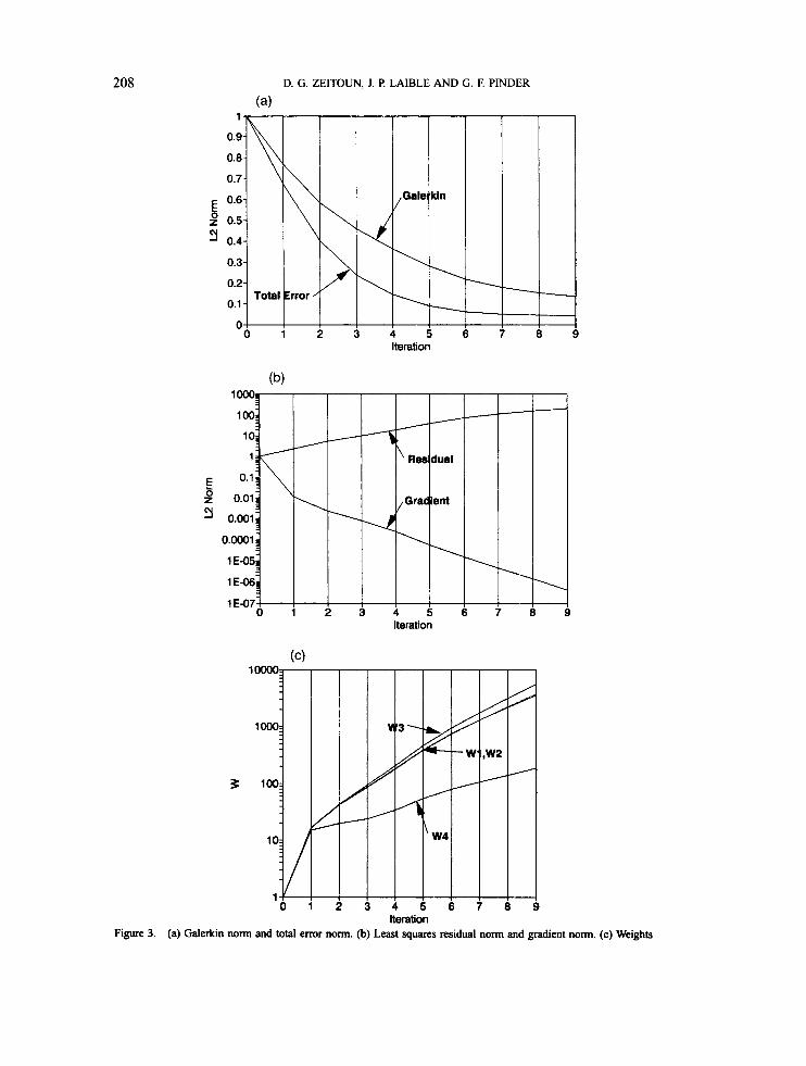
There are five weights in this problem. W, and W, are the weights for the x- and y-momentum equations respectively. W3 is associated with the continuity equation. W4 and W5 are the weights associated with the prescribed < (on r = r2) and the prescribed zero normal flow on the remaining boundaries. All weights were set initially to 1.0. The weight W5 (normal flow condition) was fixed at 1.0 and the optimizatiorn process was carried out to determine Wl-W4 that minimize the auxiliary function Yw Tables I and I1 and Figure 3 summarize the results. In Table I the numerical values of various norms are listed for each step of the optimization. The residual norm is defined as the L2-norm of the vector { e } evaluated at each of the active domain collocation points and at the boundary collocation points. The Galerkin norm is actually the value of Ya as defined by equation (35). The values in the exact column are the L2-norm ofthe total error. This is simply the s u m ofthe squares of the difference between the numerical and analytical solutions evaluated at the same points used for the residual norm. The gradient norm is the L2-norm of {aQ.,/asi} as defined by the left-hand side of equation (42). The four norms are also plotted in Figures 3(a) and 3(b). Owing to their varying magnitudes, the values are normalized with respect to the values in the first row of Table I. The corresponding weights at each iteration are listed in Table I1 and plotted in Figure 3(c). For this test problem the iteration procedure was carried out until the gradient norm was less than lop6 of the initial gradient norm.

208

- w

D. G. ZEITOUN, J. F! LAIBLE AND G . F. PINDER

(a)

,w2

/’ /

Iteration

(b)

Iteration

(c)

Iteration Figure 3. (a) Galerkin norm and total error norm. (b) Least squares residual norm and gradient norm. (c) Weights


6.2. Discussion

The significance of these results is best illustrated by Figure 3(a). We see that weights that reduce the Galerkin norm also reduce the exact (total error) norm. It is thus apparent that in the absence of any knowledge of an analytic solution we can rely on the Galerkin norm as a guide to decreasing the total error of the solution. The importance of this result is hrther appreciated by considering Figure 3(b), where it can be seen that the L2 residual norm of the least squares method is actually increasing as the solution becomes more accurate. Figure 3(c) reveals that although the total error can be reduced by minimizing the Galerkin norm, the weights continue to increase ({ Asi} becomes constant) while the gradient {a@,,/asi} approaches zero. This implies that the second derivatives are zero and that we are approaching a plateau of neutral stability. The selection of weights larger than those that mark the onset of this plateau has a negligible affect on the numerical solution. At the extreme condition of very large weights, however, it is conceivable that ill conditioning may cause the solution to begin to degenerate.

7. CONCLUSIONS

An alternative least squares method for the solution of a first-order system of partial differential equations has been presented. The new feature of the method is a systematic methodology for the determination of the optimal weights appearing in the weighted least squares method.

The results obtained for the solution of the two-dimensional shallow water equations show a superiority of the new approach when compared with the classical least squares and Galerkin methods.

APPENDIX: PROOF OF THEOREM 2

Symbols and notations introduced in Section 4 are used in this appendix. The proof consists of a comparison between two minimization problems. The first optimization

problem does not involve weights and may be formulated as follows. Find the vector solution a,, of dimension php of the minimization problem

Min [RL(a, x)I2dn J, subject to Li(x)a -5 = 0,

subject to Bl(x)a - gr = 0, i = 2 , . . . , P , 1 = 1, . . . ,pb

(problem a), where &(a,@ is defined as the residual of the first equation:

The second minimization problems corresponds to the penalty formulation of problem formulated as

and may be

(problem R,).

210 D. G. ZEITOUN, J. P. LAIBLE AND G . F. PINDER

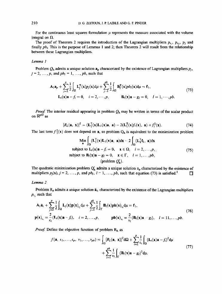
For the continuous least squares formulation p represents the measure associated with the volume integral on R.

The proof of Theorem 2 requires the introduction of the Lagrangian multipliers pe , , p , , p j and finally pbl. This is the purpose of Lemmas 1 and 2; then Theorem 2 will result fiom the relationship between these Lagrangian multipliers.

Lemma 1

Problem Qh admits a unique solution ap characerized by the existence of Lagrangian multipliers pi, j = 2, , . . , p, and pbl = 1, . . . , pb, such that

Li(x)a -J; = 0, i = 2,. . . ,p, BI(x)a - gl = 0, 1 = 1, . . . ,pb.

Proof: The interior residual appearing in problem Qh may be written in terms of the scalar product on [ w P ~ as

[&(a, X)l2 = (LT(x)L1(x)a, a) - 2(LT(xK(x), a) +f2(x). (74) The last temf:(x) does not depend on a, so problem Q h is equivalent to the minimization problem

(LT(x)Ll (x)a, a)dx - 2

(75) subject to Li(x)a -J; = 0, x E R, i = 2,. . . ,p,. subject to Bl(x)a - g1 = 0, x E r, 1 = 1,. . . ,pb,

(problem g,). The quadratic minimization problem Qk admits a unique solution ap characterized by the existence of multipliers pJ{x), j = 2, . . . , p, and pb,, 1 = 1, . . . , pb, such that equation (73) is satisfied.'

Lemma 2

Problem R,, admits a unique solution sic characterized by the existence of the Lagrangian multipliers pe, such that

Proof: Define the objective function of problem R,, as

(77)

FIRST-ORDER HYPERBOLIC SYSTEMS 21 1

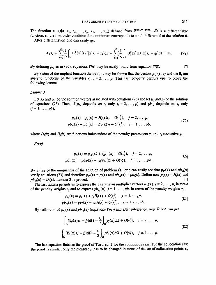
The function a--tf(a, cl, €2, ..., cp, vl, ..., vpb) defined fiom R@(D+lr-pb)+R is a differentiable function, so the first-order condition for a minimum corresponds to a null differential at the solution a.

After differentiation one can easily get

By defining pCi as in (76), equations (76) may be easily found from equation (78). 0 By virtue of the implicit function theorem, it may be shown that the vectors p E (x, c) and the a, are

analytic functions of the variables cj, j = 2, . . . , p . This last property permits one to prove the following lemma.

Lemma 3

Let aE and p., be the solution vectors associated with equations (76) and let ap andp, be the solution of equations (73). Then, if p s depends on cj only (j = 2, . . . , p ) and pb, depends on vj only (j= 1, . . . , p b),

(79) P ~ , ( x ) -pi(.) = 4 ( x ) c j + o($), j = 2,. . . ,P ,

pbV,(x) -pbr(x) = Di(x)vr + ~ ( v : ) , 1 = 1,. . . ,pb,

where Q(x) and Hj(x) are functions independent of the penalty parameters v1 and c, respectively.

Pmof

By virtue of the uniqueness of the solution of problem Q,,, one can easily see that p~,{x) and pbvdx) verify equations (73) and therefore p&) = p,{x) and pb&) = pbl(x). Define now pr,ix) = H,{x) and

0 The last lemma permits us to express the Lagrangian multiplier vectors p,, (x), j = 2, . . . , p , in terms

pbll(x) = Ddx). Lemma 3 is proved.

of the penalty weights c, and to express pb, (x), j = 1, . . . , pb, in terms of the penalty weights v,:

The last equation finishes the proof of Theorem 2 for the continuous case. For the collocation case the proof is similar, only the measure p has to be changed in terms of the set of collocation points xi,

212 D. G. ZEITOUN, J. P. LAIBLE AND G. F. PMDER

i = 1 , . . . , k, for the interior collocation points and x i , i = k + 1, . . . , m, for the boundary collocation points:

REFERENCES

1. R. Glowinski, Numerical Methods for Nonlinear Variational Problems, Springer, Berlin, 1986. 2. J. Bensabat and D. G. Zeitoun, ‘A least-squares formulation for the solution of transport problems’, Int. j. nume,: methods

fluids, 10, 623436. 3. T. J. R. Hughes, L. P. F m c a and G. M. Hulbert, ‘A new finite element formulation for computational fluid dynamics: the

Galerkidleast squares method for advective4iffisive equations’, Comput. Methods Appl. Mech. Eng. 73, 173-1 89 (1 989). 4. E. D. Eason, ‘A review of least-squares methods for solving partial differential equations’, Int. j . nume,: methods eng., 10,

1021-1046 (1976). 5 . K. 0. Friedrichs, ‘Symmetric positive differential equations’, Commun. Pure Appl. Math., 11, 333418 (1958). 6. L. Lapidus and G. F. Pinder, Numerical Solution of Partial Differential Equations in Science and Engineering, Wiley, New

7. P. Lesaint and I? A. Raviart, ‘Finite element collocation methods for first order systems’, Math. Cornput., 33, 891-918

8. A. K. Aziz and J. L. Liu, ‘A weighted least squares method for the backward-forward heat equation’, SIAM1 Nume,: Anal.,

9. J. H. Bramble and A. H. Shatz, ‘Least squares methods for 2mth order elliptic boundary value problems’, Math. Cornput., 25,

York, 1982.

(1 979).

28, 156167 (1991).

1-32 (1971). 10. W. L. Wendland, Elliptic Systems in the Plane, Pitan, London, 1979. 11. A. K. Aziz, R. B. Kellogg and A. B. Stephens, ‘Least squares methods for elliptic systems’, Math. Comput, 44, 53-70

12. G. F. Carey and B. N. Jiang, ‘Least-squares finite elements for first order hyperbolic systems’, Int. j . nume,: methods eng.,

13. B. N. Jiang and G. F. Carey, ‘A stable least-squares finite element method for non-linear hyperbolic problems’, Int. j. nume,:

14. B. N. Jiang and G. F. Carey, ‘Least-squares finite element methods for compressible Euler equations’, Int. j. nume,: methods

15. J. I? Laible and G. F. Pinder, ‘Least squares collocation solution of differential equations on irregularly shaped domains using

16. J. F? Laible and G. F. Pinder, ‘Solution of the shallow water equations by least-squares collocation’, Adv. Water Resources

17. I? A. Raviart and J. M. Thomas, Intmduction a I ’Analyse Numerique des Equations a u Derivees Partielles, Masson, Paris,

18. T.-F. Chen, ‘On least-squares approximations to compressible flow problems’, Numea Methods PDEs, 2 , 207-228 (1986). 19. D. G. Zeitoun, J. I? Laible and G. F. Pinder, ‘An iterative least- squares solution for boundary value problems’, Int. j . numeE

20. D. R. Lynch and W. G. Gray, ‘Analytic solutions for computer flow model testing’, 1 HydmuI. Div., ASCE, 104, 1409-1428

(1985).

26, 81-93 (1988).

methodsfluids, 8, 933-942 (1988).

fluids, 10, 557-568 (1990).

orthogonal meshes’, Nume,: Methods PDEs, 5 , (1989).

Rex, submitted.

1988.

methods eng., submitted.

(1978).

A weighted least squares method for first-order hyperbolic systems

Documents

Transcript of A weighted least squares method for first-order hyperbolic systems