Orthogonal series density estimation in a disaggregation scheme
Upload
independentCategory
view
0download
0
arX
iv:1
407.
1372
v1 [
mat
h.N
A]
5 J
ul 2
014
DIRECT METHODS FOR SOLVING POSITIVE DEFINITE TOTALLEAST SQUARES PROBLEMS USING ORTHOGONAL MATRIX
DECOMPOSITIONS
NEGIN BAGHERPOUR ∗ AND NEZAM MAHDAVI-AMIRI †
Abstract. In several process control contexts such as estimation of mass inertia matrix instructural control problems, an overdetermined linear system of equations with multiple right handside vectors arises with the constraint that the unknown matrix be symmetric and positive definite.The coefficient and the right hand side matrices are respectively named data and target matrices.A similar mathematical problem is also devised for modeling a deformable structure. A number ofoptimization methods were proposed for solving such problems, in which the data matrix is unreal-istically assumed to be error free. Here, considering error in measured data and target matrices, wepropose a new approach based on the use of a newly defined error function to solve a positive definiteconstrained total least squares problem. We provide a comparison of our proposed approach andtwo existing methods, the interior point method and a method based on quadratic programming.Numerical test results show that the new approach leads to smaller standard deviations of the errorentries and smaller effective rank as desired for control problems. Furthermore, in a comparativestudy, using the Dolan-More performance profiles, we show the proposed approach to be more effi-cient .
Key words. Total least squares, positive definite constraints, structural control, deformablestructures, correlation matrix
AMS subject classifications. 65F05, 65F20, 49M05
1. Introduction. Computing a symmetric positive definite solution of an overde-termined linear system of equations arises in a number of physical problems such asestimating the mass inertia matrix in the design of controllers for solid structuresand robots; see, e.g., [1], [2], [3]. Modeling a deformable structure also leads to sucha mathematical problem; see, e.g., [4]. The problem turns into finding an optimalsolution of the system
DX ≃ T,(1.1)
where D,T ∈ Rm×n, with m ≥ n, are given and a symmetric positive definite matrix
X ∈ Rn×n is to be computed as a solution of (1.1). In some special applications,
the data matrix D has a simple structure, which may be taken into considerationfor efficiently organized computations. Estimation of the covariance matrix and com-putation of the correlation matrix in finance are two such examples where the datamatrices are respectively block diagonal and the identity matrix; see, e.g., [5].A number of least squares formulations have been proposed for the physical problems,which may be classified as ordinary and total least squares problems.Also, single or multiple right hand side least squares may arise. With a single righthand side, we have an overdetermined linear system of equations Dx ≃ t, whereD ∈ R
m×n, t ∈ Rm×1, with m ≥ n, are known and the vector x ∈ R
n×1 is to becomputed. In an ordinary least squares formulation, the error is only attributed to
∗Faculty of Mathematical Sciences, Sharif University of Technology, Tehran, Iran, ([email protected]).
†Faculty of Mathematical Sciences, Sharif University of Technology, Tehran, Iran,([email protected]).
1

2 NEGIN BAGHERPOUR AND NEZAM MAHDAVI-AMIRI
t. So, to minimize the corresponding error, the following mathematical problem isdevised:
min ‖∆t‖
s.t. Dx = t+∆t.(1.2)
There are a number of methods for solving (1.2), identified as direct and iterativemethods. A well known direct method is based on using the QR factorization of thematrix D [6]. An iterative method has also been introduced in [7] for solving (1.2)using the GMRES algorithm.In total least squares formulation, however, errors in both D and t are considered. Inthis case, the corresponding mathematical problem is posed to be (see, for example,[8], [9])
min ‖[∆D,∆t]‖
s.t. (D +∆D)x = t+∆t.(1.3)
Both direct [10] and iterative [11] methods have been presented for solving (1.3).A least squares problem with multiple right hand side vectors can also be formulatedas an overdetermined system of equations DX ≃ T , where D ∈ R
m×n, T ∈ Rm×k,
with m ≥ n, are given and the matrix X ∈ Rn×k is to be computed. With ordinary
and total least squares formulations, the respective mathematical problems are:
min ‖∆T ‖
s.t. DX = T +∆T
X ∈ Rn×k(1.4)
and
min ‖[∆D,∆T ]‖
s.t. (D +∆D)X = T +∆T
X ∈ Rn×k.(1.5)
Common methods for solving (1.4) are similar to the ones for (1.2); see, e.g., [6],[7]. Solving (1.5) is possible by using the method described in [12], based on the SVDfactorization of the matrix [D, T ]. Connections between ordinary least squares andtotal least squares formulations have been discussed in [13].Here, we consider an specific case of the total least squares problem with multipleright hand side vectors. Our goal is to compute a symmetric positive definite solutionX ∈ R
n×n to the overdetermined system of equations DX ≃ T , where both matricesD and T may contain errors. Several approaches have been proposed for this prob-lem, commonly considering the ordinary least squares formulation and minimizingthe error ‖∆T ‖F over all n × n symmetric positive definite matrices, where ‖.‖F isthe Frobenious norm. Larson [14] discussed a method for solving a positive definiteleast squares problem considering the corresponding normal system of equations. Heconsiders both symmetric and positive definite least squares problems. Krislock [4]proposed an interior point method for solving a variety of least squares problemswith positive semi-definite constraints. Woodgate [15] described a new algorithm forsolving a similar problem in which a symmetric positive semi-definite matrix P is com-puted to minimize ‖F − PG‖, with known F and G. Hu [16] presented a quadratic
Positive Definite Total Least Squares 3
programming approach to handle the positive definite constraint. In her method, theupper and lower bounds for the entries of the target matrix can be given as extraconstraints. In real measurements, however, both the data and target matrices maycontain errors; hence, the total least squares formulation appears to be appropriate.The rest of our work is organized as follows. In Section 2, we define a new errorfunction and discuss some of its characteristics. A method for solving the resultingoptimization problem with the assumption that D has full column rank is presentedin Section 3. In Section 4, we generalize the method to the case of data matrix havingan arbitrary rank. In Section 5, a detailed discussion is provided on computationalcomplexity of both methods. Computational results and comparisons with availablemethods are given in Section 6. Section 7 gives our concluding remarks.
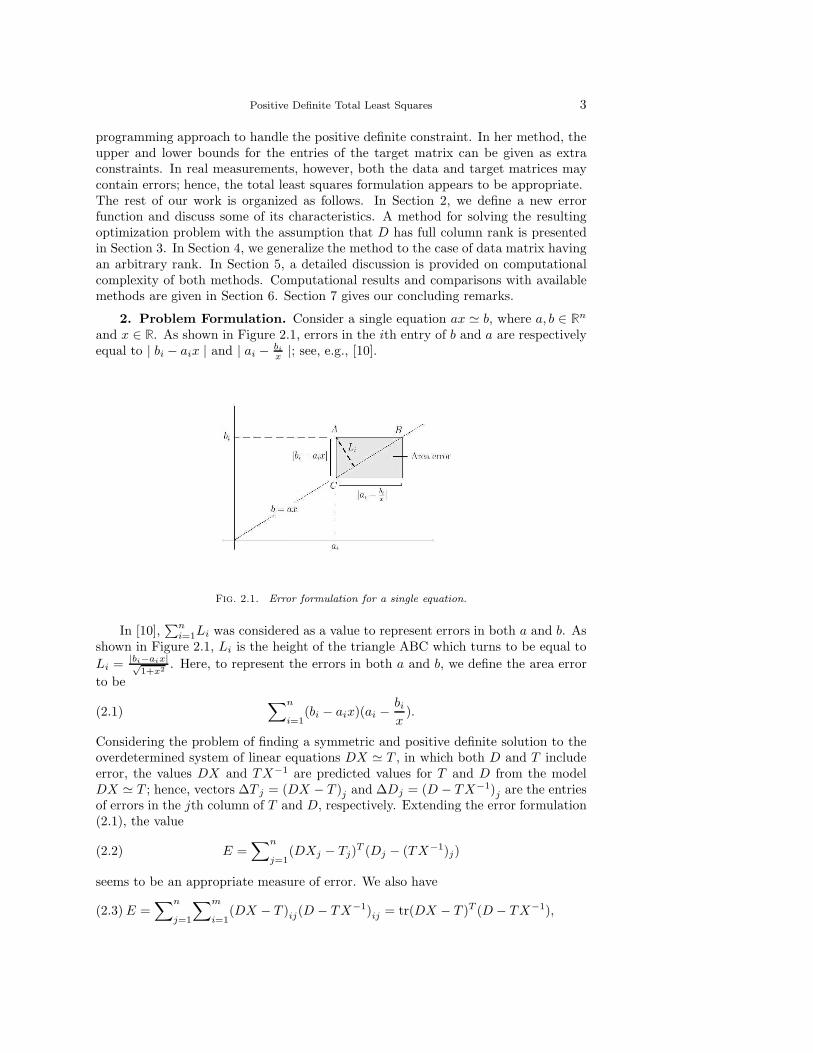
2. Problem Formulation. Consider a single equation ax ≃ b, where a, b ∈ Rn
and x ∈ R. As shown in Figure 2.1, errors in the ith entry of b and a are respectivelyequal to | bi − aix | and | ai −
bix|; see, e.g., [10].
Fig. 2.1. Error formulation for a single equation.
In [10],∑n
i=1Li was considered as a value to represent errors in both a and b. Asshown in Figure 2.1, Li is the height of the triangle ABC which turns to be equal to
Li =|bi−aix|√
1+x2. Here, to represent the errors in both a and b, we define the area error
to be
∑n
i=1(bi − aix)(ai −
bi
x).(2.1)
Considering the problem of finding a symmetric and positive definite solution to theoverdetermined system of linear equations DX ≃ T , in which both D and T includeerror, the values DX and TX−1 are predicted values for T and D from the modelDX ≃ T ; hence, vectors ∆T j = (DX − T )j and ∆Dj = (D − TX−1)j are the entriesof errors in the jth column of T and D, respectively. Extending the error formulation(2.1), the value
E =∑n
j=1(DXj − Tj)
T (Dj − (TX−1)j)(2.2)
seems to be an appropriate measure of error. We also have
E =∑n
j=1
∑m
i=1(DX − T )ij(D − TX−1)ij = tr(DX − T )T (D − TX−1),(2.3)

4 NEGIN BAGHERPOUR AND NEZAM MAHDAVI-AMIRI
with tr(.) standing for trace of a matrix. Therefore, the problem can be formulatedas
minX≻0
tr(DX − T )T (D − TX−1),(2.4)
where X is symmetric and by X ≻ 0, we mean X is positive definite.
Note. An appropriate characteristic of the error formulation proposed by (2.3) isthat its value is nonnegative and it is equal to zero if and only if DX = T .
3. Mathematical Solution. Here, we are to develop an algorithm for solving(2.4) with the assumption that D has full column rank. The following results arewell-known; see, e.g., [18].
Lemma 3.1. For an invertible matrix P ∈ Rn×n and arbitrary matrices Y ∈
Rn×n, A ∈ R
m×n and B ∈ Rn×m we have
(1) tr(Y ) = tr(P−1Y P ).(2) tr(AB) = tr(BA).
Using Lemma 3.1, we have
tr(DX − T )T (D − TX−1) = tr(DTDX +X−1T TT )− 2tr(T TD).
So, (2.4) can be written as
min tr(AX +X−1B),(3.1)
where A = DTD and B = T TT and the symmetric and positive definite matrix X isto be computed.To explain our method for solving (3.1), we present the following theorems.
Theorem 3.2. The solution X∗ for problem (3.1) satisfies
X∗AX∗ = B.
Proof. Let Φ(X) = tr(AX + X−1B). The first order necessary conditions for(3.1) [19] is obtained to be,
∇Φ(X) = A−X−1BX−1 = 0,
or equivalently,
X∗AX∗ = B,(3.2)
where X∗ is symmetric and positive definite.
The following theorem helps us to check whether the first order necessary condi-tions defined in Theorem 3.2 are sufficient for optimality.

Positive Definite Total Least Squares 5
Theorem 3.3. (Sufficient optimality conditions) [19] Consider the opti-mization problem
min f(X)
s.t. g(X) = 0.(3.3)
Suppose that L(X,λ) = f(X) − λg(X) is the corresponding Lagrangian and ∇2L isits Hessian matrix. If the matrices X∗ and λ∗ satisfy the KKT necessary conditionsand sT∇2L(X∗, λ∗)s is positive for each feasible direction s from X∗, then X∗ is astrict local solution for (3.3). Also, if f(X) is strictly convex and {X | g(X) = 0} isconvex, then X∗ is the unique global solution.
Corollary 3.4. For each X∗ satisfying the first order necessary conditions of(3.1), the sufficient optimality conditions described in Theorem 3.3 are satisfied andsince Φ(X) = tr(AX +X−1B) is convex on the cone of symmetric positive definitematrices, we can confirm that the symmetric positive definite matrix satisfying theKKT necessary conditions mentioned in Theorem 3.2 is the unique global solution of(3.1).
Effective methods for computing the positive definite matrix satisfying KKT con-ditions have yet to be developed. Later, we will show how to compute such a matrixby using two well-known matrix decompositions.
Note. (Cholesky decomposition) A Cholesky decomposition [6] of a symmetricpositive definite matrix A ∈ R
n×n is a decomposition of the form A = RTR, whereR, known as the Cholesky factor of A, is an n×n invertible upper triangular matrix.
Note. (Spectral decomposition) [6] All eigenvalues of a symmetric matrix, A ∈Rn×n, are real and there exists an orthonormal matrix with columns representing the
corresponding eigenvectors. Thus, there exist an orthogonal matrix U with columnsequal to the eigenvectors of A and a diagonal matrixD containing the eigenvalues suchthat A = UDUT . Also, if A is positive definite, then all of its eigenvalues are positive,and so we can set D = S2. Thus, spectral decomposition for a symmetric positivedefinite matrix A is a decomposition of the form A = US2UT , with UTU = UUT = I
and S a diagonal matrix.
Theorem 3.5. Assume D,T ∈ Rm×n with m ≥ n are known and rank(D) =
rank(T ) = n. Let A = DTD and B = T TT . Let the Cholesky factor of A beR. Define the matrix Q = RBRT and compute its spectral decomposition, that is,Q = RBRT = US2UT . Then, (3.1) has a unique solution, given by
X∗ = R−1USUTR−T .
Proof. Based on Theorem 3.3 and the afterwards discussion, it is sufficient toshow that X∗ satisfies the necessary optimality conditions, X∗AX∗ = B. Substitut-ing X∗, we have
X∗AX∗ = R−1USUTR−TRTRR−1USUTR−T
= R−1US2UTR−T = R−1RBRTR−T = B.

6 NEGIN BAGHERPOUR AND NEZAM MAHDAVI-AMIRI
We are now ready to outline the steps of our proposed algorithm.
ALGORITHM 1. Solving positive definite total least squares problemusing Cholesky Decomposition (PDTLS-Chol).
Inputs: D,T ∈ Rm×n.
Outputs: X∗ and error E = tr(DX∗ − T )T (D − TX∗−1).
(1) Let A = DTD and compute its Cholesky decomposition: A = RTR.
(2) Let Q = RBRT , where B = T TT and compute the spectral decomposition ofQ, that is, Q = US2UT .
(3) Set X∗ = R−1USUTR−T .
(4) Set E = tr(DX∗ − T )T (D − TX∗−1).
The iterative methods proposed in [4], [5] and [16] generate a sequence convergingto the solution. Unlike these methods, ALGORITHM 1 computes the solution of(2.4) directly. This is the main advantage of ALGORITHM 1, which turns to re-quire less computing time in obtaining a solution.The following theorem shows that the spectral decomposition of A can also be usedto solve (3.1).
Theorem 3.6. Let A = DTD and B = T TT with D,T ∈ Rm×n, m ≥ n and
rank(D) = n. Let the spectral decomposition of A be A = US2UT . Define the matrixQ = SUTBUS and compute its spectral decomposition, Q = SUTBUS = U S2UT .Then, the unique minimizer of (3.1) is
X∗ = US−1U SUTS−1UT .
Proof. Similar to the proof of Theorem 3.5, it is sufficient to show that the men-tioned X∗ satisfies X∗AX∗ = B. Substituting X∗, we have
X∗AX∗ = US−1U SUTS−1UTUS2UTUS−1U SUTS−1UT
= US−1U S2UTS−1UT = US−1SUTBUSS−1UT = B.
Next, based on Theorem 3.6, we outline an algorithm for solving (2.4).
ALGORITHM 2. Solving positive definite total least squares problemusing spectral Decomposition (PDTLS-Spec) .
Inputs: D,T ∈ Rm×n.
Outputs: X∗ and error E = tr(DX∗ − T )T (D − TX∗−1).
(1) Let A = DTD and compute its spectral decomposition: A = US2UT .
(2) Let Q = SUTBUS, where B = T TT and compute the spectral decomposition of
Positive Definite Total Least Squares 7
Q, that is, Q = U S2UT .
(3) Set X∗ = US−1U SUTS−1UT .
(4) Set E = tr(DX∗ − T )T (D − TX∗−1).
4. Solution of a Rank Deficient Data Matrix. Since the data matrix D isusually produced from experimental measurements, the assumption that rank(D) = n
may not hold. In Section 4.1, we generalize ALGORITHM 1 for solving (2.4), as-suming that rank(D) = r < n. It will be shown that, in general, (2.4) may not have aunique solution. Hence, in section 4.2 we discuss finding a particular solution of (2.4)having desirable characteristics for control problems.
4.1. General solution. Based on theorems 3.2 and 3.3, a symmetric positivedefinite matrix X∗ is a solution of (2.4) if and only if
X∗AX∗ = B.(4.1)
Therefore, in the following, we discuss how to find a symmetric positive definite ma-trix X∗ satisfying (4.1).
Let the spectral decomposition of A be A = U
(
S2 00 0
)
UT , where S2 ∈ Rr×r is a
diagonal matrix having the positive eigenvalues of A as its diagonal entries. Substi-tuting the decomposition in (4.1), we get
X∗U
(
S2 00 0
)
UTX∗ = B.(4.2)
Since U is orthonormal, (4.2) can be written as
UTX∗U
(
S2 00 0
)
UTX∗U = UTBU.
Then, letting X = UTXU and B = UTBU , we have
X
(
S2 00 0
)
X = B.(4.3)
Thus, the matrix X = UXUT is a solution of (2.4) if and only if X is symmetricpositive definite and satisfies (4.3).
Substituting the block form X =
(
Xrr Xr,n−r
Xn−r,r Xn−r,n−r
)
, where Xrr ∈ Rr×r, Xr,n−r =
XTn−r,r ∈ R
r×(n−r) and Xn−r,n−r ∈ R(n−r)×(n−r), in (4.3) leads to
(
XrrS2Xrr XrrS
2Xr,n−r
Xn−r,rS2Xrr Xn−r,rS
2Xr,n−r
)
= B =
(
Brr Br,n−r
Bn−r,r Bn−r,n−r
)
,(4.4)
which is satisfied if and only if
XrrS2Xrr = Brr,(4.5a)
XrrS2Xr,n−r = Br,n−r,(4.5b)
8 NEGIN BAGHERPOUR AND NEZAM MAHDAVI-AMIRI
Xn−r,rS2Xr,n−r = Bn−r,n−r.(4.5c)
Let D = S and suppose T satisfies T T T = Brr. Consider problem (2.4) correspondingto the data and target matrices D and T as follows:
minX≻0
tr(DX − T )T (D − T X−1).(4.6)
We know from theorems 3.2 and 3.3 that the necessary and sufficient optimalityconditions for the unique solution of problem (4.6) implies (4.5a). Thus, Xrr can becomputed using ALGORITHM 1 for the input arguments D and T . Substitutingthe computed Xrr in (4.5b), the linear system of equations
XrrS2Xr,n−r = Br,n−r(4.7)
arises, where Xrr, S2 ∈ R
r×r are known and Xr,n−r ∈ Rr×(n−r) is to be computed.
Since Xrr is positive definite and S2 is invertible, the coefficient matrix of the linearsystem (4.7) is invertible and Xr,n−r can be uniquely computed.
It is clear that since X is symmetric, Xn−r,r is the same as XTr,n−r. Now, we check
whether the computed Xn−r,r and Xr,n−r satisfy (4.5c). Inconsistency of (4.5c) meansthat there is no symmetric positive definite matrix satisfying (4.5a)-(4.5c), and if so,(2.4) has no solution. Thus, in solving an specific positive definite total least squaresproblem with rank deficient data and target matrices, a straightforward method toinvestigate the existence of solution is to check whether (4.5c) for the given dataand target matrices. On the other hand, for numerical results, it is necessary togenerate meaningful test problems. Hence, in the following lemma, we investigate thenecessary and sufficient conditions for satisfaction of (4.5c). We later use the resultsof this lemma to generate consistent test problems in Section 6.
Lemma 4.1. Let the spectral decompositions of A and B be determined as A =
U
(
S2 00 0
)
UT and B = V
(
∑20
0 0
)
V T , where S2,∑2
∈ Rr×r and rank(A) =
rank(B) = r. The necessary and sufficient condition for satisfaction of (4.5c) is that
V = U
(
Q 00 P
)
,(4.8)
where Q ∈ Rr×r and P ∈ R
(n−r)×(n−r) satisfy QQT = QTQ = I and PPT = PTP =I.
Proof. From (4.5a), we have
X−1rr S−2X−1
rr = B−1rr ,(4.9)
and from (4.5b), we get
Xr,n−r = S−2X−1rr Br,n−r,(4.10)
Xn−r,r = Bn−r,rX−1rr S−2.(4.11)
Manipulating (4.5c) with (4.9) and (4.10), we get
Bn−r,rB−1rr Br,n−r = Bn−r,n−r.(4.12)

Positive Definite Total Least Squares 9
Considering the block form U =(
Ur Un−r
)
, where Ur ∈ Rn×r and Un−r ∈
Rn×(n−r), we have
B = UTBU =
(
UrT
Un−rT
)
B(
Ur Un−r
)
=
(
UrTBUr Ur
TBUn−r
Un−rTBUr Un−r
TBUn−r
)
.
Rewriting (4.12), we get
Un−rTBUr(Ur
TBUr)−1
UrTBUn−r = Un−r
TBUn−r,(4.13)
which is equivalent to
BUr(UrTBUr)
−1Ur
TB = B+,(4.14)
where B+ is the pesudo-inverse of B.Based on well-known properties of the pesudo-inverse [6], (4.14) is satisfied if and onlyif
Ur(UrTBUr)
−1Ur
T = B+ = Vr
∑−2Vr
T ,(4.15)
where Vr ∈ Rn×r is composed of the first r columns of V .
Multiplying (4.15) by UrT and Ur respectively on the left and right, and substituting
the spectral decomposition of B, we get
(UrTVr
∑2Vr
TUr)−1
= UrTB+Ur = Ur
TVr
∑−2Vr
TUr.(4.16)
Letting M = UrTVr, we get
(M∑2
MT )−1
= M∑−2
MT .(4.17)
Since M has full rank, we get
M−T∑−2
M−1 = M∑−2
MT .(4.18)
Now, (4.18) holds if and only if
MTM = I.(4.19)
This leads to
(UrTVr)
TUr
TVr = VrTUrUr
TVr = I.(4.20)
Since U is orthonormal, we have UUT = UrUrT + Un−rUn−r
T = I. Hence, we get
UrUrT = I − Un−rUn−r
T .(4.21)

10 NEGIN BAGHERPOUR AND NEZAM MAHDAVI-AMIRI
Substituting (4.21) in (4.20), we get
VrT (I − Un−rUn−r
T )Vr = I − VrTUn−rUn−r
TVr = I,(4.22)
which is satisfied if and only if Un−rTVr = 0. Since the columns of Ur form an
orthogonal basis for the null space of Un−rT [6], it can be concluded that each column
of Vr is a linear combination of the columns of Ur. Thus,
Vr = UrQ(4.23)
is a necessary condition for (4.19) to be satisfied, and, since both Ur and Vr haveorthogonal columns, Q ∈ R
r×r satisfies QQT = QTQ = I. On the other hand, weknow from the definition of the spectral decomposition that V V T = UUT = I. Thus,
VrVrT + Vn−rVn−r
T = I,
UrUrT + Un−rUn−r
T = I.(4.24)
Manipulating (4.23) with (4.24), we get
Vn−rVn−rT = Un−rUn−r
T ,(4.25)
which holds if and only if there exists a matrix P ∈ R(n−r)×(n−r) such that PPT =
PTP = I and
Vn−r = PUn−r.(4.26)
It can be concluded from (4.23) and (4.26) that V = U
(
Q 00 P
)
, where QQT =
QTQ = I and PPT = PTP = I.
Corollary 4.2. The matrices P and Q defined in Lemma 4.1 can set to berotation matrices [6] to satisfy
PPT = PTP = I,
QQT = QTQ = I.
Thus, to compute a target matrix, T , satisfying Lemma 4.1, it is sufficient to firstcompute V from (4.8) with Q ∈ R
r×r and P ∈ R(n−r)×(n−r) arbitrary rotation ma-
trices and U as defined in Lemma 4.1 and then set T = U
(∑
00 0
)
V T , where
U ∈ Rm×m and
∑
∈ Rr×r are arbitrary orthonormal and diagonal matrices. Thus,
problem (2.4) has a solution if and only if the data and target matrices satisfy (4.23).In this case, Xrr, Xr,n−r and its transpose Xr,n−r are respectively computed from
(4.5a) and (4.5b). Hence, the only remaining step is to compute Xn−r,n−r so that
X is symmetric and positive definite. Definition3 gives a straightforward idea forcomputing Xn−r,n−r.
We know that X is symmetric positive definite if and only if there exists an invertiblelower triangular matrix L ∈ R
n×n so that
X = LLT ,(4.27)

Positive Definite Total Least Squares 11
where L is lower triangular and nonsingular. Considering the block forms X =(
Xrr Xr,n−r
Xn−r,r Xn−r,n−r
)
and L =
(
Lrr 0Ln−r,r Ln−r,n−r
)
, where Ln−r,r is an (n−r)×
r matrix and Lrr ∈ Rr×r and Ln−r,n−r ∈ R
(n−r)×(n−r) are invertible lower triangularmatrices, we get
(
Xrr Xr,n−r
Xn−r,r Xn−r,n−r
)
=
(
Lrr 0Ln−r,r Ln−r,n−r
)(
LrrT Ln−r,r
T
0 Ln−r,n−rT
)
.(4.28)
Thus,
Xrr = LrrLrrT ,(4.29a)
Xr,n−r = LrrLn−r,rT ,(4.29b)
Xn−r,r = Ln−r,rLrrT ,(4.29c)
Xn−r,n−r = Ln−r,rLn−r,rT + Ln−r,n−rLn−r,n−r
T .(4.29d)
Therefore, to compute a symmetric positive definite X, (4.29a)–(4.29d) must be satis-fied. Let Xrr = LLT be the Cholesky decomposition of Xrr. Lrr = L satisfies (4.29a).Substituting Lrr in (4.29b), Ln−r,r
T is computed uniquely by solving the resultinglinear system. Since (4.29c) is transpose of (4.29b), it does not give any additionalinformation. Finally, to compute a matrix Xn−r,n−r to satisfy (4.29d), it is sufficientto choose an arbitrary lower triangular nonsingular matrix Ln−r,n−r and substitute it
in (4.29d). The resulting Xn−r,n−r gives a symmetric positive definite X as follows:
X =
(
Xrr Xr,n−r
Xn−r,r Xn−r,n−r
)
.
Now, based on the above discussion, we outline the steps of our algorithm for solving(2.4) in the case rank(D) = r < n.
ALGORITHM 3. Solving positive definite total least squares problemwith rank deficient data matrix using spectral decomposition (PDTLS-RD-Spec).
Inputs: D,T ∈ Rm×n.
Outputs: X∗ and error E = tr(DX∗ − T )(D − TX∗−1).
(1) Let A = DTD and compute its spectral decomposition: A = U
(
S2 00 0
)
UT .
(2) Let B = T TT and B = UTBU .(3) Compute rank(D) = r and let Brr = B(1 : r, 1 : r), Br,n−r = B(1 : r, r + 1 : n)
and Bn−r,n−r = B(r + 1 : n, r + 1 : n).
(4) Let D = S and assume T satisfies Brr = T T T .(5) Call ALGORITHM 1 with input parameters D = D and T = T , and let
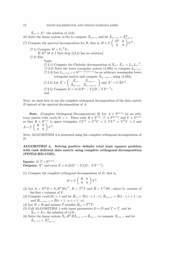
12 NEGIN BAGHERPOUR AND NEZAM MAHDAVI-AMIRI
Xrr = X∗, the solution of (4.6).(6) Solve the linear system (4.5b) to compute Xr,n−r and let Xn−r,r = XT
r,n−r.
(7) Compute the spectral decomposition for B, that is, B = V
(
D2 00 0
)
V T .
(7.1) Compute M = UrTVr.
If MTM 6= I then stop {(2.4) has no solution}(7.2) Else
begin(7.2.1) Compute the Cholesky decomposition of Xrr: Xrr = LrrLrr
T .(7.2.2) Solve the lower triangular system (4.29b) to compute Ln−r,r.(7.2.3) Let Ln−r,n−r ∈ R
(n−r)×(n−r) be an arbitrary nonsingular lower
triangular matrix and compute Xn−r,n−r using (4.29d).
(7.2.4) Let X =
(
Xrr Xr,n−r
Xn−r,r Xn−r,n−r
)
and X∗ = UXUT .
(7.2.5) Compute E = tr(DX∗ − T )(D − TX∗−1).end.
Next, we show how to use the complete orthogonal decomposition of the data matrixD instead of the spectral decomposition of A.
Note. (Complete Orthogonal Decomposition) [6] Let A ∈ Rm×n be an arbi-
trary matrix with rank(A) = r. There exist R ∈ Rr×r, U ∈ R
m×m and V ∈ Rn×n
so that R ∈ Rr×r is upper triangular, UUT = UTU = I, V V T = V TV = I and
A = U
(
R 00 0
)
V T .
Next, ALGORITHM 4 is presented using the complete orthogonal decomposition ofD.
ALGORITHM 4. Solving positive definite total least squares problemwith rank deficient data matrix using complete orthogonal decomposition(PDTLS-RD-COD).
Inputs: D,T ∈ Rm×n.
Outputs: X∗ and error E = tr(DX∗ − T )(D − TX∗−1).
(1) Compute the complete orthogonal decomposition of D, that is,
D = U
(
R 00 0
)
V T .
(2) Let A = DTD = VrRTRVr
T , B = T TT and B = V TBV , where Vr consists ofthe first r columns of V .
(3) Compute rank(D) = r and let Brr = B(1 : r, 1 : r), Br,n−r = B(1 : r, r + 1 : n)
and Bn−r,n−r = B(r + 1 : n, r + 1 : n).
(4) Let D = R and assume T satisfies Brr = T T T .(5) Call ALGORITHM 1 with input parameters D = D and T = T , and let
Xrr = X∗, the solution of (4.6).(6) Solve the linear system XrrR
TRXr,n−r = Br,n−r to compute Xr,n−r and let
Xn−r,r = XTr,n−r.
Positive Definite Total Least Squares 13
(7) Compute the spectral decomposition for B, that is, B = W
(
D2 00 0
)
WT .
(7.1) Compute M = UrTVr.
If MTM 6= I then stop {(2.4) has no solution}(7.2) Else
begin(7.2.1) Compute the Cholesky decomposition of Xrr: Xrr = LrrLrr
T .(7.2.2) Solve the lower triangular system (4.29b) to compute Ln−r,r.(7.2.3) Let Ln−r,n−r ∈ R
(n−r)×(n−r) be an arbitrary nonsingular lower
triangular matrix and compute Xn−r,n−r using (4.29d).
(7.2.4) Let X =
(
Xrr Xr,n−r
Xn−r,r Xn−r,n−r
)
and X∗ = UXUT .
(7.2.5) Compute E = tr(DX∗ − T )(D − TX∗−1).end.
In the following, we discuss finding a particular solution of (2.4) having proper char-acteristics.
4.2. Particular solution. Based on algorithms 3 and 4, in the case of rank de-ficient data matrix, problem (2.4) has infinitely many solutions. These solutions aregenerated by having different choices of Ln−r,n−r ∈ R
(n−r)×(n−r), an arbitrary non-singular lower triangular matrix. Here, we describe how to find a particular solutionX having desired characteristics for control problems. Effective rank and conditionnumber, defined in the next two definitions, are two important characteristics.
Definition 4.3. (Effective Rank [23]) The effective rank of a matrix X ∈ Rn×n
is defined to ber(X) = traceX
‖X‖2
.
Note. For X, a symmetric positive definite matrix, by using the spectral decomposi-tion X = US2UT , the effective rank of X is
r(X) =s21+...+s2
n
s21
,
where s2i is the ith diagonal entry of S2.
Definition 4.4. (Condition Number [6]) Assume that X ∈ Rn×n is a symmetric
positive definite matrix. With the spectral decomposition X = US2UT the conditionnumber of X is defined to be
κ(X) =s21
s2n
.
We will later make use of common constraints on condition number and effectiverank of the particular solution of (2.4), as significant features for control problems.
Proposition 4.5. As proper characteristics for control problems, it is appropri-ate for a solution X of (2.4) to satisfy the following conditions:
(1) r(X) be as low as possible, [23] and(2) κ(X) < K. [24]
Note. Considering the definition X = UTXU , it can be concluded that X andX have the same effective ranks and condition numbers. Thus, in the following wediscuss on r(X) and κ(X) instead of r(X) and κ(X) in Preposition 4.5.

14 NEGIN BAGHERPOUR AND NEZAM MAHDAVI-AMIRI
We know from (4.28) that
X =
(
LrrLrrT LrrLn−r,r
T
Ln−r,rLrrT Ln−r,rLn−r,r
T + I
)
+
(
0 0
0 Ln−r,n−rLn−r,n−rT − I
)
.
Defining
F =
(
LrrLrrT LrrLn−r,r
T
Ln−r,rLrrT Ln−r,rLn−r,r
T + I
)
and
Y =
(
0 0
0 Ln−r,n−rLn−r,n−rT − I
)
,
we get X = F+Y . Note that F =
(
Lrr 0Ln−r,r I
)(
LTrr LT
n−r,r
0 I
)
has full rank. In
Lemma 4.6 below, we review some properties of eigenvalues to simplify the specifiedconditions in Proposition 4.5.
Lemma 4.6. [25] Let A and B be two n × n symmetric positive semi-definitematrices. The following inequalities hold for eigenvalues of A, B and A + B, whereλi(.) denotes the ith largest eigenvalue of a matrix:
(1) λ1(A+B) ≥ λ1(B),(2) λ1(A+B) ≤ λ1(A) + λ1(B),(3) λn(A+B) ≥ λn(A) + λn(B).
Using Lemma 4.6, we get
r(X) =λ1(F ) + ...+ λn(F ) + λ1(Y ) + ...+ λn−r(Y )
λ1(X)
≤λ1(F ) + ...+ λn(F ) + λ1(Y ) + ...+ λn−r(Y )
λ1(Y ).
κ(X) =λ1(X)
λn(X)≤
λ1(F ) + λ1(Y )
λn(F ) + λn(Y ),(4.30)
where λn(Y ) = 0, and since F is nonsingular, λn(F ) 6= 0.Considering (4.30), since F and thus λi(F ) are fixed, the sufficient condition to sat-isfy condition (1) in Proposition 4.5 is to set λ1(Y ) as large as possible and chooseλ2(Y ), λ3(Y ), ... and λn−r(Y ) to be small positive values to decrease the value ofr(X). The largest possible value for λ1(Y ) to satisfy condition (2) in Proposition 4.5is Kλ1(F )− λn(F ).Thus, to compute a particular solution of (2.4) satisfying Proposition 4.5, it is suffi-cient to let Xn−r,n−r have a spectral decomposition of the form Xn−r,n−r = WΣ2WT ,with σ2
1 = Kλ1(F )− λn(F ) and σ2i , i = 1, 2, . . . , n− r, having small positive values.
In Section 5, we will compare the computational complexity of PDTLS-RD-Spec andPDTLS-RD-COD. Also, based on the reported numerical results in Section 6, wemake a comparison of the required computing time by the algorithms.
5. Computational Complexity. Here, we study the computational complexityof our algorithms for solving the positive definite total least squares problem.
5.1. Full column rank data matrix case. The computational complexitiesof PDTLS-Chol and PDTLS-Spec presented in Section 3 for the case of full column

Positive Definite Total Least Squares 15
rank data matrix are respectively given in tables 5.1 and 5.2; for details about theindicated computational complexities, see [6].
Table 5.1
Needed computations in PDTLS-Chol and the corresponding computational complexities.
Computation Time complexity
A = DTD 12mn2
Cholesky decomposition for A ∈ Rn×n n3
6B = TTT 1
2mn2
RB n3
2
Q = RBRT n3
4Spectral decomposition of Q ∈ R
n×n 4n3
R−1 n3
2
USUT n3
2+ n2
R−1USUT n3
2
X∗ = R−1USUTR−T n3
4
Total time complexity NPDTLS−Chol = mn2 + 203n3
Table 5.2
Needed computations in PDTLS-Spec and the corresponding computational complexities.
Computation Time complexity
A = DTD 12mn2
Spectral decomposition for A ∈ Rn×n 4n3
B = TT T 12mn2
SUT n2
Q = SUTBUS 32n3
Spectral decomposition of Q ∈ Rn×n 4n3
S−1 n
US−1 n2
USUT n3
2+ n2
X∗ = US−1U SUTS−1UT . 32n3
Total time complexity NPDTLS−Spec = mn2 + 232n3
Comparing the resulting complexities of NPDTLS−Chol and NPDTLS−Spec, asgiven in tables 5.1 and 5.2, it can readily be concluded that, independent of the matrixsize, the computational complexity of PDTLS-Chol is lower than that of PDTLS-Spec.
5.2. Rank deficient data matrix case. The computational complexities ofPDTLS-RD-Spec and PDTLS-RD-COD presented in Section 4 for the case of rankdeficient data matrix are respectively provided in tables 5.3 and 5.4.

16 NEGIN BAGHERPOUR AND NEZAM MAHDAVI-AMIRI
Table 5.3
Needed computations in PDTLS-RD-Spec and the corresponding computational complexities.
Computation Time complexity
A = DTD 12mn2
Spectral decomposition for A ∈ Rn×n 4n3
B = TTT 12mn2
B = UTBU 32n3
NPDTLS−Chol(r × r diagonal data matrix) 4r3 + 3r2
Solving the linear system (4.5b) (n3
3+ n2)(n− r)
Spectral decomposition for B ∈ Rn×n 2n3
Cholesky decomposition for Xrrr3
6
Solving the lower triangular system (4.29b) (n2
2)(n− r)
Computing Xn−r,n−r from (4.29d) r(n− r)2 +(n−r)3
2Total time complexity NPDTLS−RD−Spec
∗
∗ : NPDTLS−RD−Spec = mn2 + 152 n
3 + 256 r3 + (n
3
3 + n2)(n − r) + (n2
2 )(n − r) +
r(n− r)2+ (n−r)3
2 .
Table 5.4
Needed computations in PDTLS-RD-COD and the corresponding computational complexities.
Computation Time complexity
Complete orthogonal decomposition for D ∈ Rm×n 4mn2
−43n3
A = DTD = VrRTRVr
T nr2 + r3
2B = TTT 1
2mn2
B = V TBV 32n3
NPDTLS−Chol(r × r) 152r3
Solving the linear system (4.5b) (n3
3+ n2)(n − r)
Spectral decomposition for B ∈ Rn×n 2n3
Cholesky decomposition for Xrrr3
6
Solving the lower triangular system (4.29b) (n2
2)(n − r)
Computing Xn−r,n−r from (4.29d) r(n− r)2 +(n−r)3
2Total time complexity NPDTLS−RD−COD
∗
∗ : NPDTLS−RD−COD = 92mn2+nr2+ 13
6 n3+ 496 r
3 +(n3
3 +n2)(n− r)+ (n2
2 )(n−
r) + r(n− r)2+ (n−r)3
2 .
Considering the results for NPDTLS−RD−Spec and NPDTLS−RD−COD in tables5.3 and 5.4, we have
N PDTLS−RD−Spec −NPDTLS−RD−COD
= (mn2 +15
2n3 +
25
6r3)− (
9
2mn2 + nr2 +
13
6n3 +
49
6r3)
= −4mn2 +16
3n3 − nr2 − 4r3.
We can see that if 4mn2+nr2 +4r3 > 163 n
3, then PDTLS-RD-Spec has a lower com-putational complexity; otherwise, the computational complexoty of PDTLS-RD-COD
Positive Definite Total Least Squares 17
is lower.Thus, based on the above study, the computational complexity of PDTLS-Chol islower than that of PDTLS-Spec, for all matrix sizes. But, for the case of rank de-ficient data matrix, depending on the matrix size and rank, one of the algorithmsPDTLS-RD-Spec and PDTLS-RD-COD may have a lower computational complexity.
6. Numerical Results. Here, some numerical results are reported. We madeuse of MATLAB 2012b in a Windows 7 machine with a 3.2 GHz CPU and a 4 GBRAM. We generated random test problems with random data and target matrices.These random matrices were produced using the rand command in MATLAB. Thecommand rand(m,n) generates an m × n matrix with uniformly distributed randomentries in the interval [0, 1]. The random test problems were classified into problemswith full column rank data matrix and problems with rank deficient data matrix.In Section 6.1, we report the numerical results corresponding to full column rank datamatrices. For a given matrix size, we generated 50 random test problems and reportedthe average time and the average error, E values in tables 6.1, 6.2 and 6.3. To studythe effect of using Cholesky or spectral decompositions in our proposed approach, weconstructed the Dolan-More performance profile.The Dolan-More performance profile was introduced in [26] to compare the perfor-mance of different algorithms on solving a given problem. Here, we used the newversion of this performance profile which is derivative free [27].The Dolan-More performance profile can be generated for different parameters. Sincea desired feature in estimation of mass inertia matrix is that the standard deviationvalue of the resulting error matrix in T be as low as possible, we compare the requiredtime and the standard deviation values in PDTLS-Chol and PDTLS-Spec; hence, wepresent the Dolan-More performance profile for these parameters. It can be concludedfrom the generated performance profiles in figures 6.1 and 6.2 that the required timeby PDTLS-Chol is lower than that of PDTLS-Spec.Also, to compare our proposed approach (PDTLS) with the interior point method(IntP), discussed in [4], and the method proposed by Hu in [16] (HuM) we con-structed the corresponding Dolan-More performance profiles in figures 6.3 and 6.4 toconfirm that our proposed method generates solutions with lower standard deviationvalues in lower computing time.
In Section 6.2, the numerical results for test problems with rank deficient datamatrices are reported. In such test problems, generating anm×n random data matrixwith column rank r is necessary. Hence, we first used the command
R = rand(m,n)
to generate a full column rank m × n random matrix, and then set the data matrixD to be equal to its singular value decomposition (SVD) of rank r,
[U , S , V ] = svd(R)D = U(:, 1 : r) ∗ S(1 : r, 1 : r) ∗ (V ′)(1 : r, :).
Also, the target matrix T was computed from Corollary 4.2.For a given matrix size and rank, we generated 50 test problems. Similar to Section6.1, we report the average required time and average value of error, E in tables 6.4,6.5 and 6.6. We also studied the effect of using complete orthogonal decompositionand spectral decomposition in the proposed approach. To compare the efficiency ofthese decompositions, we constructed the Dolan-More performance profiles of requiredtimes and standard deviation values for the numerical results produced by PDTLS-
18 NEGIN BAGHERPOUR AND NEZAM MAHDAVI-AMIRI
RD-Spec and PDTLS-RD-COD in figures 6.5 and 6.6. Our proposed approach wasalso compared with the other available methods based on the Dolan-More perfor-mance profiles as presented in figures 6.7 and 6.8. Also, we computed the particularsolution of (2.4), choosing appropriate values for eigenvalues of the matrix Y based onthe discussion at the end of Section 4 to satisfy conditions given in Proposition 4.5.We presented the Dolan-More performance profiles of effective rank and conditionnumber in figures 6.9 and 6.10 confirming the efficiency of our proposed algorithm ingenerating solutions with lower values of effective rank and condition number.Numerical results also confirmed the effectiveness of ALGORITHM 1 through 4 inproducing more accurate solutions with lower standard deviation values in lower times.
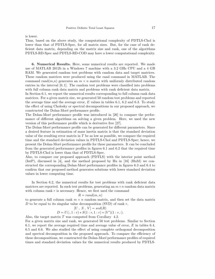
6.1. Full column rank data matrix. In Table 6.1, the average error value,E = tr(DX∗ − T )(D − TX∗−1), and the average required time (in seconds) arereported for (PDTLS-Chol) and (PDTLS-Spec). The first two columns of this ta-ble contain the matrix size, the third to sixth columns give the time and error for(PDTLS-Chol) and the time and error for (PDTLS-Spec), respectively.
Table 6.1
Average time and error values for PDTLS-Chol and PDTLS-Spec.
m n Time E Time E(PDTLS-Chol) (PDTLS-Chol) (PDTLS-Spec) (PDTLS-Spec)
100 10 0.0021 1.6191E+002 0.0014 1.6191E+002100 50 0.0017 7.2274E+002 0.0022 7.2274E+002100 100 0.0058 1.2388E+003 0.0072 1.2388E+0031000 100 0.0089 1.6258E+004 0.0104 1.6258E+0041000 200 0.0434 3.1684E+004 0.0505 3.1684E+004
The reported results in Table 6.1 show that (PDTLS-Chol) is faster in comput-ing the solution. Also, the Dolan-More performance profile for the required timesby these algorithms given in Figure 6.1 confirms this result. However, based on theDolan-More performance profile for the standard deviation values showed in Figure6.2, there is no significant difference between the standard deviation values generatedby the two algorithms.

Positive Definite Total Least Squares 19
1 1.5 2 2.5 30
0.2
0.4
0.6
0.8
1
PDTLS−CholPDTLS−Spec
Fig. 6.1. The Dolan-More performance profile (comparing the required time by PDTLS-Choland PDTLS-Spec).
100
101
102
0
0.2
0.4
0.6
0.8
1
PDTLS−CholPDTLS−Spec
Fig. 6.2. The Dolan-More performance profile (comparing the standard deviation value forPDTLS-Chol and PDTLS-Spec).
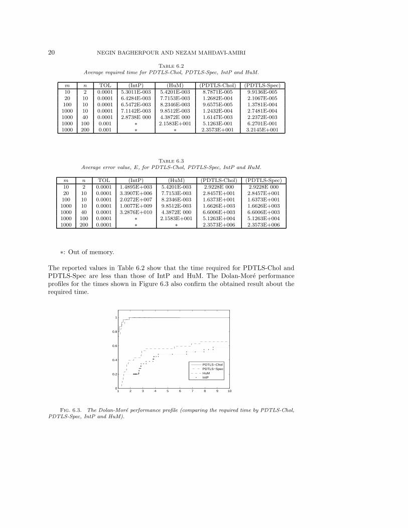
In the following, we compare our proposed approach with the available methods.In tables 6.2 and 6.3, the average required time (in seconds) and the average errorvalue, E = tr(DX∗ − T )(D − TX∗−1), are reported for IntP [7], HuM [16], PDTLS-Chol and PDTLS-Spec.The first two columns give the matrix size, the third column is the value of TOL forIntP and HuM methods and the remaining columns give the average error value, andthe average required time (in seconds) for IntP, HuM, PDTLS-Chol and PDTLS-Spec,respectively.
20 NEGIN BAGHERPOUR AND NEZAM MAHDAVI-AMIRI
Table 6.2
Average required time for PDTLS-Chol, PDTLS-Spec, IntP and HuM.
m n TOL (IntP) (HuM) (PDTLS-Chol) (PDTLS-Spec)10 2 0.0001 5.3011E-003 5.4201E-003 8.7871E-005 9.9136E-00520 10 0.0001 6.4284E-003 7.7153E-003 1.2682E-004 2.1067E-005100 10 0.0001 6.5472E-003 8.2346E-003 9.6575E-005 1.3781E-0041000 10 0.0001 7.1142E-003 9.8512E-003 1.2432E-004 2.7481E-0041000 40 0.0001 2.8738E 000 4.3872E 000 1.6147E-003 2.2372E-0031000 100 0.001 ∗ 2.1583E+001 5.1263E-001 6.2701E-0011000 200 0.001 ∗ ∗ 2.3573E+001 3.2145E+001
Table 6.3
Average error value, E, for PDTLS-Chol, PDTLS-Spec, IntP and HuM.
m n TOL (IntP) (HuM) (PDTLS-Chol) (PDTLS-Spec)10 2 0.0001 1.4895E+003 5.4201E-003 2.9228E 000 2.9228E 00020 10 0.0001 3.3907E+006 7.7153E-003 2.8457E+001 2.8457E+001100 10 0.0001 2.0272E+007 8.2346E-003 1.6373E+001 1.6373E+0011000 10 0.0001 1.0077E+009 9.8512E-003 1.6626E+003 1.6626E+0031000 40 0.0001 3.2876E+010 4.3872E 000 6.6006E+003 6.6006E+0031000 100 0.0001 ∗ 2.1583E+001 5.1263E+004 5.1263E+0041000 200 0.0001 ∗ ∗ 2.3573E+006 2.3573E+006
∗: Out of memory.
The reported values in Table 6.2 show that the time required for PDTLS-Chol andPDTLS-Spec are less than those of IntP and HuM. The Dolan-More performanceprofiles for the times shown in Figure 6.3 also confirm the obtained result about therequired time.
1 2 3 4 5 6 7 8 9 100
0.2
0.4
0.6
0.8
1
PDTLS−CholPDTLS−SpecHuMIntP
Fig. 6.3. The Dolan-More performance profile (comparing the required time by PDTLS-Chol,PDTLS-Spec, IntP and HuM).

Positive Definite Total Least Squares 21
Also, considering the Dolan-More performance profiles for standard deviationvalues in Figure 6.4, the standard deviation values for numerical results generated byPDTLS-Chol and PDTLS-Spec are considerably lower than those of IntP and HuM.
0 200 400 600 800 10000
0.2
0.4
0.6
0.8
1
PDTLS−CholPDTLS−SpecHuMIntP
Fig. 6.4. The Dolan-More performance profile (comparing the standard deviation values forPDTLS-Chol, PDTLS-Spec, IntP and HuM).
6.2. Rank deficient data matrix. Here, we report the obtained numerical re-sults, similar to Section 6.1, for test problems with rank deficient data matrix.In Table 6.4 and figures 6.5 and 6.6, we see numerical results obtained by PDTLS-RD-Spec and PDTLS-RD-COD.In Table 6.4, the average error value and the required time for PDTLS-RD-Spec andPDTLS-RD-COD are reported.
Table 6.4
Average time and error values for PDTLS-RD-Spec and PDTLS-RD-COD.
m n r Time E Time E(Spec) (Spec) (COD) (COD)
100 10 5 3.6377E-004 1.8733E+002 6.3001E-004 1.8733E+002100 50 20 1.4125E-003 2.0468E+003 1.6243E-003 2.0468E+003100 100 50 5.1234E-003 3.9126E+003 5.9146E-003 3.9126E+0031000 100 50 6.3142E-003 2.0047E+004 1.2843E-002 1.6258E+0041000 200 100 3.0763E-002 5.8443E+004 4.3702E-002 5.8443E+004
In figures 6.5 and 6.6, the Dolan-More performance profiles for time and standarddeviation values of PDTLS-RD-Spec and PDTLS-RD-COD are shown.

22 NEGIN BAGHERPOUR AND NEZAM MAHDAVI-AMIRI
1 1.5 2 2.5 30
0.2
0.4
0.6
0.8
1
PDTLS−SpecPDTLS−COD
Fig. 6.5. The Dolan-More performance profile (comparing the required time by PDTLS-RD-Spec and PDTLS-RD-COD).
100
101
102
0
0.2
0.4
0.6
0.8
1
PDTLS−SpecPDTLS−COD
Fig. 6.6. The Dolan-More performance profile (comparing the standard deviation values forPDTLS-RD-Spec and PDTLS-RD-COD).
These results show that PDTLS-RD-Spec computes the solution faster, but thereis no significant difference in the obtained standard deviations.In tables 6.5 and 6.6 and figures 6.7 and 6.8, our proposed approach is compared withother methods.The required times and standard deviations for IntP, HuM, PDTLS-RD-Spec andPDTLS-RD-COD are reported in tables 6.5 and 6.6 respectively.
∗: Out of memory.
In figures 6.7 and 6.8, the Dolan-More performance profiles for time and standarddeviation values confirm that PDTLS-RD-Spec and PDTLS-RD-COD compute moreaccurate solutions with lower values of standard deviation in lower times.

Positive Definite Total Least Squares 23
Table 6.5
Average required time for PDTLS-RD-Spec, PDTLS-RD-COD, IntP and HuM.
m n r TOL (IntP) (HuM) (PDTLS-RD- (PDTLS-RD-Spec) COD)
100 10 5 0.0001 3.0312E-002 3.1056E-002 3.4886E-004 8.9062E-004100 20 10 0.0001 2.0231E-001 2.3417E-001 4.1248E-004 6.7299E-004100 50 10 0.0001 2.2054E-001 2.8615E-001 3.8361E-004 7.1187E-004100 50 20 0.0001 2.1953E-001 3.5758E-001 3.8099E-004 7.0380E-0041000 10 5 0.0001 2.3651E 000 4.1172E 000 2.5414E-004 7.3529E-0041000 40 20 0.0001 ∗ 1.1362E+001 1.6741E-003 8.8415E-0021000 100 50 0.0001 ∗ ∗ 1.1092E-002 7.6443E-001
Table 6.6
Average error value, E, for PDTLS-RD-Spec, PDTLS-RD-COD, IntP and HuM.
m n r TOL (IntP) (HuM) (PDTLS-RD- (PDTLS-RD-Spec) COD)
100 10 5 0.0001 1.2143E+003 1.6157E+003 2.1366E+002 2.1366E+002100 20 10 0.0001 2.8547E+004 3.0147E+004 3.5939E+002 3.5939E+002100 50 10 0.0001 1.6149E+006 5.2981E+006 2.4805E+003 2.4805E+003100 50 20 0.0001 8.9124E+007 2.5746E+008 2.5505E+003 2.5505E+0031000 10 5 0.0001 6.4572E+009 1.7364E+010 1.4846E+003 1.4846E+0031000 40 20 0.0001 ∗ 9.1654E+011 2.5643E+004 2.5643E+0041000 100 50 0.0001 ∗ ∗ 5.8416E+006 5.8416E+006
10 20 30 40 50 60 70 80 90 1000
0.2
0.4
0.6
0.8
1
PDTLS−SpecPDTLS−CODHuMIntP
Fig. 6.7. The Dolan-More performance profile (comparing the required time by PDTLS-RD-Spec, PDTLS-RD-COD, IntP and HuM).
10 20 30 40 50 60 70 80 90 1000
0.2
0.4
0.6
0.8
1
PDTLS−SpecPDTLS−CODHuMIntP
Fig. 6.8. The Dolan-More performance profile (comparing the standard deviation values forPDTLS-RD-Spec, PDTLS-RD-COD, IntP and HuM).

24 NEGIN BAGHERPOUR AND NEZAM MAHDAVI-AMIRI
The Dolan-More performance profiles for effective rank and condition numberpresented in figures 6.9 and 6.10 confirm the efficiency of our proposed algorithm ingenerating solutions with lower values of effective rank and condition number.
0 0.5 1 1.5 2 2.5 3
x 106
0
0.2
0.4
0.6
0.8
1
PDTLS−SpecHuMIntP
Fig. 6.9. The Dolan-More performance profile (comparing the values of effective rank forPDTLS-RD-Spec, IntP and HuM).
0 20 40 60 80 1000
0.2
0.4
0.6
0.8
1
PDTLS−SpecHuMIntP
Fig. 6.10. The Dolan-More performance profile (comparing the values of condition number forPDTLS-RD-Spec, IntP and HuM).
Considering the numerical results reported in this section, for the data matrix D
having full column rank, we observe:
(1) Required time by PDTLS-Chol is lower than that of PDTLS-Spec.(2) Required time and standard deviation values for PDTLS-Chol and PDTLS-Spec
are considerably lower than those of IntP and HuM.
And, if the data matrix is rank deficient, we observe:
(1) Required time by PDTLS-RD-Spec is lower than that of PDTLS-RD-COD.(2) Required time and standard deviation values for PDTLS-RD-Spec and PDTLS-
RD-COD are considerably lower than those of the methods IntP and HuM, andthe standard deviation values for PDTLS-RD-Spec is lower than those of theother three methods.
Positive Definite Total Least Squares 25
(3) PDTLS-RD-Spec can generate particular solutions with considerably lower valuesof effective rank and condition number than IntP and HuM.
7. Concluding Remarks. We proposed a new approach to solve positive def-inite total least squares problems, offering three main desirable features. First, con-sideration of our proposed error in both the data and target matrices admits a morerealistic problem formulation. Second, the proposed algorithm computes the exactsolution directly, and, as shown by numerical results obtained on randomly gener-ated test problems, is more efficient than two other existing methods. The generatedDolan-More performance profiles also confirm the efficiency of our proposed algo-rithms. Finally, numerical results showed lower standard deviation of the error in thetarget matrix and lower values of effective rank and condition number, as desired forcontrol problems. The new approach lead us to develop the algorithms PDTLS-Choland PDTLS-Spec for the case of data matrix having full column rank, and PDTLS-RD-Spec and PDTLS-RD-COD for the case of rank deficient data matrix. The nu-merical results also showed that PDTLS-Chol, using the Cholesky decomposition,computes the solution faster in the case of full column rank data matrix. However,PDTLS-RD-Spec showed to be more efficient when the data matrix is rank deficient.
ACKNOWLEDGEMENT. The authors thank Research Council of Sharif Uni-versity of Technology for supporting this work.
REFERENCES
[1] H. Hu and I. Olkin, A numerical procedure for finding the positive definite matrix closest to apatterned matrix, Statistical and Probability Letters, 12, 1991, pp. 511-515.
[2] P. Poignet and M. Gautier, Comparison of Weighted Least Squares and Extended Kalman Fil-tering Methods for Dynamic Identification of Robots, Proceedings of the IEEE Conferenceon Robotics and Automation, San Francisco, CA, USA, 2000, pp. 3622-3627.
[3] J. McInroy and J. C. Hamann, Design and control of flexure jointed hexapods, IEEE Trans.Robotics and Automation, 16(4), 2000, pp. 372-381.
[4] N. G.Krislock, Numerical Solution of Semidefinite Constrained Least Squares Problems, M. Sc.Thesis, University of British Colombia, 2003.
[5] N. J. Higham, Computing the nearest correlation matrix (A problem from finance), MIMSEPrint: 2006.70, http://eprints.ma.man.ac.uk/, 2006.
[6] C. F. Van Loan and G. Golub, Matrix Computation, 4th edition, JHU Press, 2012.[7] K. Hayami, J. F. Yin and T. Ito, GMRES method for least squares problems, SIAM. J. Matrix
Anal. and Appl., 31(5), 2010, pp. 2400-2430.[8] C. C. Paige and Z. Strakos, Scaled total least squares fundamentals, Numer. Math., 91, 2000,
pp. 117-146.[9] G. H. Golub and C. F. Van Loan, An analysis of the total least squares problem, SIAM J.
Numer. Anal., 17, 1980, pp. 883-893.[10] S. V. Huffel and J. Vandewalle, The Total Least Squares Problem: Computational Aspects and
Analysis, SIAM, 1991.[11] B. Kang, S. Jung and P. Park, A New Iterative Method for Solving Total Least Squares Problem,
Proceeding of the 8th Asian Control Conference (ASCC), Kaohsiung, Taiwan, 2011.[12] I. Hnetynkova, M. Plesinger, D.M. Sima , Z. Strakos and S. Van Huffel, The total least squares
problem in AX ≈ B, A new classification with the relationship to the classical works,SIAM J. Matrix Anal. Appl., 32(3), 2011, pp. 748-770.
[13] S. Van Huffel and J. Vandewalle, Algebraic connections between the least squares and total leastsquares problems, Numer. Math., 55, 1989, pp. 431-449.
[14] H. J. Larson, Least squares estimation of the components of a symmetric matrix, Technomet-rics, 8(2), 1966, pp. 360-362.

26 NEGIN BAGHERPOUR AND NEZAM MAHDAVI-AMIRI
[15] K. G. Woodgate, Least-squares solution of F = PG over positive semidefinite symmetric P,Linear Algebra Appl., 245, 1996, pp. 171-190.
[16] H. Hu, Positive definite constrained least-squares estimation of matrices, Linear Algebra andits Applications, 229, 1995, pp. 167-174.
[17] R. A. Horn and C. R. Johnson, Topics in Matrix Analysis, Cambridge University Press, 1991.[18] P. E. Gill, W. Murray and M. H. Wright, Numerical Linear Algebra and Optimization, Addison
Wesley, 1991.[19] J. Nocedal and S. J. Wright, Numerical Optimization, Springer, New York, 1999.[20] Y. Deng and D. Boley, On the Optimal Approximation for the Symmetric Procrustes Prob-
lems of the Matrix Equation AXB = C, Proceedings of the International Conference onComputational and Mathematical Methods in Science and Engineering, Chicago, 2007, pp.159-168.
[21] M. E. Polites, The estimation error covariance matrix for the ideal state reconstructor withmeasurement noise, NASA Technical Report, NASA TP-2881, 1988.
[22] K. B. Petersen and M. S. Pedersen, The Matrix Cookbook,http://orion.uwaterloo.ca/∼hwolkowi/matrixcookbook.pdf, 2008.
[23] R. Vershynin, Introduction to the non-asymptotic analysis of random matrices,http://arxiv.org/pdf/1011.3027v7.pdf, 2011.
[24] A. Aubry, A. D. Maio, L. Pallotta and Alfonso Farina, Maximum likelihood estimation of astructured covariance matrix with a condition number constraint, IEEE Trans. On SignalProcessing, 60(6), 2012, pp. 3004-3021.
[25] Eigenvalues and sums of Hermitian matrices, http://www.ams.org/bookstore/pspdf/gsm-132-prev.pdf,2009.
[26] E.D. Dolan and J.J. More, Performance profiles were originally introduced in Benchmarkingoptimization software with performance profiles, Mathematical Programming, 91, 2002,pp. 201-213.
[27] J. J. More and S. M. Wild, Benchmarking derivative-free optimization algorithms, SIAM J.Optim., 20, 2009, pp. 172-191.
[28] F. Alizadeh, J. Pierre, A. Heaberly and M. L. Overton, Primal-dual interior point methodsfor semidefinite programming: convergence rates, stability and numerical result, SIAM J.Optim., 8, 1998, pp. 746-768.

0 5 10 15 20 25 300
0.2
0.4
0.6
0.8
1
PSDTLSIntPPFToh

0 20 40 60 80 1000
0.2
0.4
0.6
0.8
1
CG−opGMRES−opCG−lin

0 5 10 15 20 25 30 35 400
0.2
0.4
0.6
0.8
1
PSDTLSMRTohMRRecht
Copyright © 2022 FDOKUMEN