1

iMOLSDOCK : induced-fit docking using mutually

orthogonal Latin squares (MOLS)

D. Sam Paul and N. Gautham*

* Corresponding Author – Dr. N. Gautham, n_gautham@hotmail.com

Centre of Advanced Study in Crystallography and Biophysics, University of Madras, Chennai 600025. India

KEYWORDS

Molecular docking, Induced-fit docking, peptide-protein docking, mutually orthogonal Latin

squares, receptor flexibility, side-chain flexibility, docking tool, MOLSDOCK

ABSTRACT

We have earlier reported the MOLSDOCK technique to perform rigid receptor/flexible ligand

docking. The method uses the MOLS method, developed in our laboratory. In this paper we report

iMOLSDOCK, the ‘flexible receptor’ extension we have carried out to the algorithm

MOLSDOCK. iMOLSDOCK uses mutually orthogonal Latin squares (MOLS) to sample the

conformation and the docking pose of the ligand and also the flexible residues of the receptor

protein. The method then uses a variant of the mean field technique to analyze the sample to arrive

at the optimum. We have benchmarked and validated iMOLSDOCK with a dataset of 44 peptide-

protein complexes with peptides. We have also compared iMOLSDOCK with other flexible

receptor docking tools GOLD v5.2.1 and AutoDock Vina. The results obtained show that the

method works better than these two algorithms, though it consumes more computer time.

2

Introduction

Designing organic small molecules that ‘fit’ into biological receptors is of great interest

in drug discovery research. Computational molecular docking is frequently used to imitate the

behaviour of a ligand (small peptide or small molecule) in the active pocket of receptor proteins.

The earliest method used for automated ligand docking was the DOCK program [1] which held

the conformation of the ligand and the receptor rigid but varied the orientation degrees of

freedom[2]. After that, docking algorithms which take into account conformational degrees of

the ligand as well of the receptor have been developed [3–5].

We had developed the MOLSDOCK technique[6,7] to perform rigid receptor/flexible

ligand docking. The method uses the MOLS technique, earlier developed in our laboratory[8].

Using mutually orthogonal Latin squares[9], the algorithm systematically identifies a small but

completely representative sample of the enormous multidimensional search space. The energy

values are calculated at each of the sampled points. These energy values are then analysed using

a variant of the mean field method[10] to simultaneously obtain the optimal conformation,

position and orientation of a small molecule ligand on a rigid protein receptor.

However, in the living cell, receptor proteins are not rigid, but may flex and move to

accommodate the ligand[11–13]. Significant differences in side-chain conformations occur in at

least 60% of the proteins between the apo and holo forms upon ligand binding, though main-

chain conformations are largely preserved [14]. In ~85% of the cases, side-chain changes were

observed in only three residues or less in the binding pocket [15]. Thus it may be useful to allow

for receptor flexibility, especially side-chain flexibility, as much as for the possible

conformational changes in the ligand.

3

Some of the docking programs that allow receptor flexibility are AutoDock Vina [16],

GOLD [17], GLIDE [18] and RosettaLigand [19]. AutoDock Vina [16] is a new generation

docking in which a succession of steps consisting of a mutation and a local optimization are

taken, with each step being accepted according to the Metropolis criterion. Receptor side-chains

may be chosen as flexible. GOLD [17] is a genetic algorithm-based docking tool which allows

for partial protein flexibility. GLIDE (grid-based ligand docking with energetics) uses

exhaustive systematic search approach, with approximations and truncations, to find the optimal

ligand pose. The Induced Fit Docking protocol in GLIDE docking tool [18] begins by docking

the active ligand using the GLIDE program. Prime, a protein structure prediction technique, is

then used to accommodate the ligand by reorienting nearby side-chains in the active site of the

protein. The initial implementation of RosettaLigand[19] was based on Rosetta [20], which

allowed the rigid body position and orientation of the ligand and the side-chain conformations in

the active site of the protein to be optimized simultaneously using a Monte Carlo minimization

procedure. Later RosettaLigand included backbone flexibility [21] with full side-chain

flexibility, along with simultaneous treatment of the ligand and the protein. The latest release of

RosettaLigand has included simultaneous docking of multiple flexible ligands, accounting for

receptor flexibility [22].

In this paper we report the ‘flexible receptor’ extension we have carried out to the

MOLSDOCK algorithm. We call the upgraded version of MOLSDOCK with receptor flexibility

as iMOLSDOCK. The new docking method iMOLSDOCK, uses ‘induced-fit’ side-chain

fluctuations in the selected flexible residues of the receptor protein, to account for receptor

flexibility. To benchmark iMOLSDOCK, we have applied this method to 44 test cases (protein-

peptide complexes) selected from the Protein Data Bank (PDB). We have compared the

4

performance of the present algorithm with popular flexible receptor docking tools : AutoDock

Vina[16] and GOLD v5.2.1[17]. We present the results here.

Materials and Methods

MOLSDOCK[6,7,23] is a ‘rigid receptor/flexible ligand’ docking method developed

using the MOLS method. The MOLS method has been presented in detail elsewhere[8,24–26].

Here, we give a brief description for completeness. For simplicity, we will first consider the

method as applied to the prediction of the minimum energy structure of a peptide. The

conformation space of a peptide may be defined as the set of all possible combinations of all

values of all its variable torsion angles. Thus, if there are ‘n’ such torsion angles, each which can

take up ‘m’ different values, there are mn different combinations of these values. In other words,

there are mn different conformations for the peptide. For each conformation a potential energy

may be calculated, and therefore the multi-dimensional conformational space can also be

considered to be potential energy surface of the peptide. The task then in peptide structure

prediction is to locate the minimum value on this surface, i.e. the minimum energy conformation.

A brute force search will lead to combinatorial explosion and, for peptides longer than about 15

residues, is beyond the capabilities of most current-day computers. Here, we use mutually

orthogonal Latin squares[9] to systematically choose a set of m2 points (or conformations) from

the conformational space of the peptide. The potential energy for each conformation is

calculated. The m2 energy values are then analyzed using a variant of the mean field

technique[10,27] to arrive at the conformation with the lowest energy. We note here that there

are a very large number of ways in which we can choose the m2 points[28]. Each choice can lead

to either the same, or to a different low energy structure. Previous experience[6–8,26,29] has

shown us that generating about 1,500 structures is sufficient to cover the entire conformational

5

space of a peptide or any other small molecule. The conformations so generated are clustered

together to identify the few lowest energy structures that are possible for the peptide.

The method was later extended to address the docking problem[6,7]. The peptide or

organic molecule is considered the flexible ligand, binding to a rigid receptor protein. In addition

to the variable torsion angles of the ligand, we included, in the search space, the variables for the

position and orientation of the ligand with respect to the protein. The energy function is also

modified to include the interaction energy between protein and ligand, along with the

intramolecular energy of the ligand. The method, dubbed MOLSDOCK, is suitable for all

organic small molecules, including peptides, as ligands.

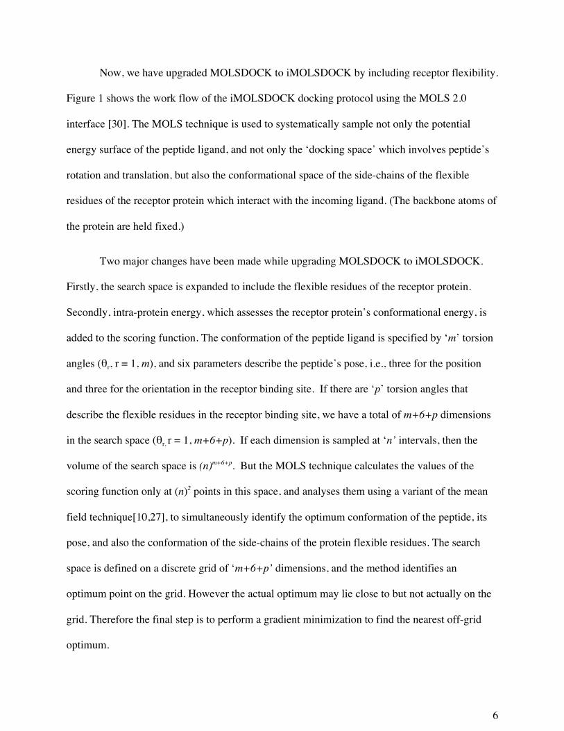
Figure 1. The workflow of iMOLSDOCK docking protocol using the MOLS 2.0 interface. If the Grid centre and flexible residues are not known, options are available in MOLS 2.0 to find them automatically.

6

Now, we have upgraded MOLSDOCK to iMOLSDOCK by including receptor flexibility.

Figure 1 shows the work flow of the iMOLSDOCK docking protocol using the MOLS 2.0

interface [30]. The MOLS technique is used to systematically sample not only the potential

energy surface of the peptide ligand, and not only the ‘docking space’ which involves peptide’s

rotation and translation, but also the conformational space of the side-chains of the flexible

residues of the receptor protein which interact with the incoming ligand. (The backbone atoms of

the protein are held fixed.)

Two major changes have been made while upgrading MOLSDOCK to iMOLSDOCK.

Firstly, the search space is expanded to include the flexible residues of the receptor protein.

Secondly, intra-protein energy, which assesses the receptor protein’s conformational energy, is

added to the scoring function. The conformation of the peptide ligand is specified by ‘m’ torsion

angles (θr, r = 1, m), and six parameters describe the peptide’s pose, i.e., three for the position

and three for the orientation in the receptor binding site. If there are ‘p’ torsion angles that

describe the flexible residues in the receptor binding site, we have a total of m+6+p dimensions

in the search space (θr, r = 1, m+6+p). If each dimension is sampled at ‘n’ intervals, then the

volume of the search space is (n)m+6+p. But the MOLS technique calculates the values of the

scoring function only at (n)2 points in this space, and analyses them using a variant of the mean

field technique[10,27], to simultaneously identify the optimum conformation of the peptide, its

pose, and also the conformation of the side-chains of the protein flexible residues. The search

space is defined on a discrete grid of ‘m+6+p’ dimensions, and the method identifies an

optimum point on the grid. However the actual optimum may lie close to but not actually on the

grid. Therefore the final step is to perform a gradient minimization to find the nearest off-grid

optimum.

7

For the peptide conformation, all its variable torsion angles, main chain and side chain,

are sampled from 0° to 360° at intervals of 10°. The orientation of the ligand in the receptor site

is specified by three angles, two of which specify the position of a rotation axis and the

remaining one is the angle of rotation about this axis, as described by Arun Prasad and Gautham

(2008). The translational position of the ligand is sampled at intervals of 0.14 Å along three

dimensions inside a cubic box of 5 Å centred at the centre of the receptor binding site. This site

is either identified from the crystal structure, if known, or may be found using the Fpocket 2.0

algorithm[30,31].

Ligand binding may induce large structural changes in the receptor protein, such as the

movement of loops[32,33] or even large domains[34,35]. In most cases, changes in backbone

structure are negligible and only side-chain reorientation occurs upon ligand binding[36,37].

Najmanovich et al. (2000) show that backbone displacements on ligand binding is of minor

importance when compared to side-chain flexibility. In iMOLSDOCK, we concentrated on the

residues lining the binding site and incorporated side-chain flexibility, where side-chains

obstructing the binding site are moved to accommodate tight binding of the ligand in the binding

site. Observations by Heringa and Argos [38] show that ligand binding induces nonrotamericity

in the preferred side-chain conformations. Zavodszky and Kuhn (2005) show that side-chain

conformational changes upon ligand binding are typically not changes between rotamers, but

mostly involve small (<15°) changes in side-chain dihedral angles relative to the original

(typically rotameric) position. Comparison between the ligand-free and ligand-bound X-ray

structures show that the side-chain dihedral angles difference is 45° or less in most (~90%) of the

cases and is 15° or less in ~80% of the cases [14]. In iMOLSDOCK we have avoided rotameric

side-chain exploration and allowed the side-chain torsion angles of the flexible residues to

8

fluctuate within the range 0° and 30° (i.e. -15° to +15° from their position in the crystal

structure). Prediction of the ligand docking pose and the receptor flexibility occur

simultaneously, resulting in an ‘induced-fit’ docking in iMOLSDOCK. If the flexible residues

that line the active site of the receptor protein are known, they may be specified explicitly. Else

residues that are within 4.0 Å from each atom of the peptide ligand are automatically selected. In

the test cases (Table 1), we have allowed a maximum of 50 flexible residues in the receptor.

The scoring function in iMOLSDOCK is the sum of the intra-molecular ligand energy,

the intra-molecular protein energy and the inter-molecular interaction energy between the ligand

and the receptor. Both the intra-molecular protein energy and intra-molecular peptide ligand

energy are calculated using the non-bonded terms of the AMBER94 force field[39]. The

intermolecular interaction energy between the protein and the ligand is calculated using the PLP

scoring function[40]. The total potential energy is the weighted sum of intra-molecular peptide

energy, intra-molecular protein energy and the intermolecular protein-peptide interaction energy.

The optimum weights were chosen to yield maximum positive correlation between the energy

and the root mean square deviation (RMSD) of the resulting docked structure with respect to the

‘native’ crystal structure. The AMBER force field is reported in units of kcal/mol[39], whereas

the PLP force field is reported in dimensionless units[40]. Therefore the total potential energy is

reported in dimensionless units.

Earlier studies using MOLS sampling for peptide prediction suggest that a MOLS sample

of 1,500 structures is exhaustive[6–8,26,29]. For iMOLSDOCK, we did an analysis to find the

number of structures sufficient for an exhaustive sampling. We generated 1,500 structures for all

the test cases (Table 1) and then clustered the structures with K-means clustering algorithm using

MMTSB toolset [41]. During the clustering procedure, the conformations were considered as

9

different, when the Ca atom superposition RMSD between them was greater than 2.0 Å. For the

tripeptide cases, 68% of the clusters had at least one representative within the first 100 structures

generated. In the case of tetrapeptides and pentapeptides all the clusters had at least one

representative structure within the first 100 structures. In the case of hexapeptide, heptapeptide

and octapeptide test cases 98%, 95% and 76% of all the clusters had at least one model within

the first 100 structures. On an average, for all the test cases, 84% of the clusters had at least one

model within the first 100 structures. For each test case, we calculated the occurrence of unique

clusters for every 100 models from 1 to 1,500 (Supplementary Figure 1). After the first 1,300

structures, no significant unique clusters occurred. Therefore generating 1,500 structures using

MOLS sampling is sufficient to identify all the low energy docked conformations of the ligand in

the protein receptor site.

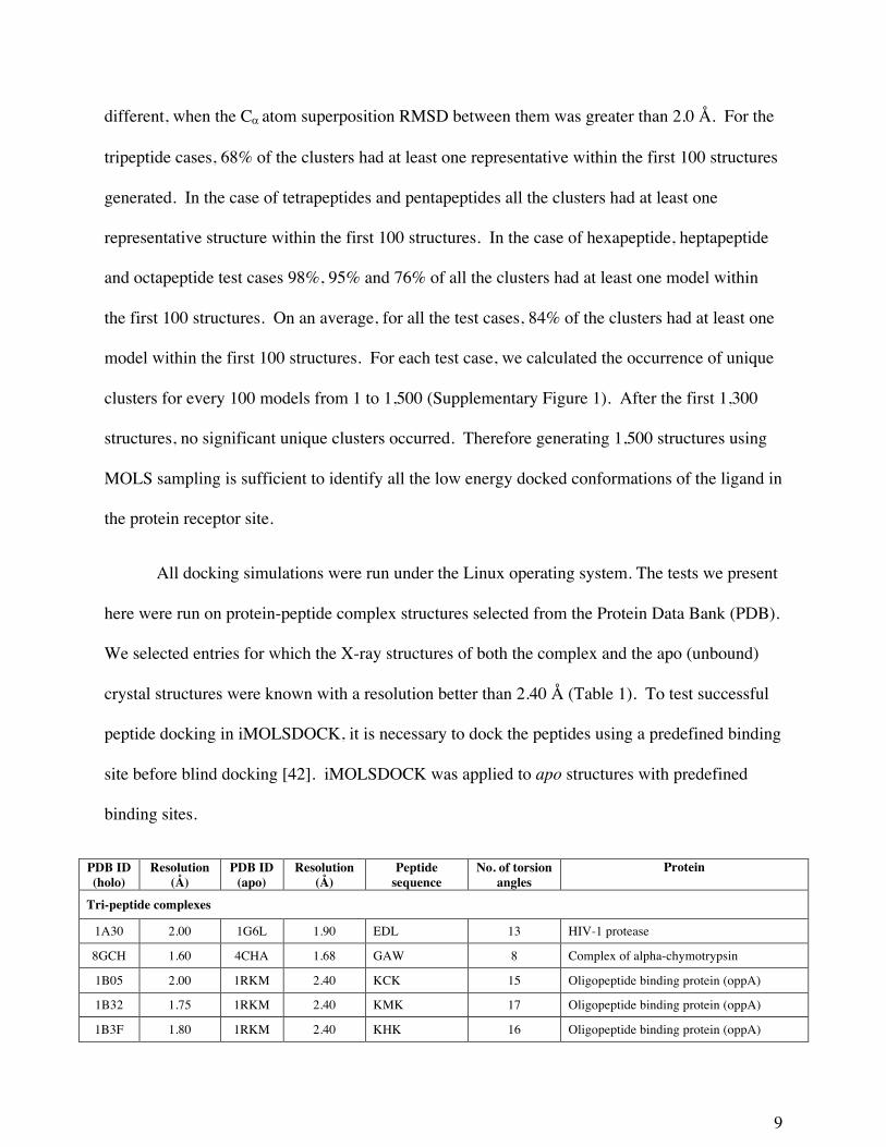
All docking simulations were run under the Linux operating system. The tests we present

here were run on protein-peptide complex structures selected from the Protein Data Bank (PDB).

We selected entries for which the X-ray structures of both the complex and the apo (unbound)

crystal structures were known with a resolution better than 2.40 Å (Table 1). To test successful

peptide docking in iMOLSDOCK, it is necessary to dock the peptides using a predefined binding

site before blind docking [42]. iMOLSDOCK was applied to apo structures with predefined

binding sites.

PDB ID (holo)

Resolution (Å)

PDB ID (apo)

Resolution (Å)

Peptide sequence

No. of torsion angles

Protein

Tri-peptide complexes

1A30 2.00 1G6L 1.90 EDL 13 HIV-1 protease

8GCH 1.60 4CHA 1.68 GAW 8 Complex of alpha-chymotrypsin

1B05 2.00 1RKM 2.40 KCK 15 Oligopeptide binding protein (oppA)

1B32 1.75 1RKM 2.40 KMK 17 Oligopeptide binding protein (oppA)

1B3F 1.80 1RKM 2.40 KHK 16 Oligopeptide binding protein (oppA)

10

1B3G 2.00 1RKM 2.40 KIK 16 Oligopeptide binding protein (oppA)

1B3L 2.00 1RKM 2.40 KGK 14 Oligopeptide binding protein (oppA)

1B46 1.80 1RKM 2.40 KPK 13 Oligopeptide binding protein (oppA)

1B4Z 1.75 1RKM 2.40 KDK 16 Oligopeptide binding protein (oppA)

1B51 1.80 1RKM 2.40 KSK 15 Oligopeptide binding protein (oppA)

1B58 1.80 1RKM 2.40 KYK 16 Oligopeptide binding protein (oppA)

1B5I 1.90 1RKM 2.40 KNK 16 Oligopeptide binding protein (oppA)

1B5J 1.80 1RKM 2.40 KQK 17 Oligopeptide binding protein (oppA)

1B9J 1.80 1RKM 2.40 KLK 16 Oligopeptide binding protein (oppA)

1JET 1.20 1RKM 2.40 KAK 14 Oligopeptide binding protein (oppA)

1JEU 1.25 1RKM 2.40 KEK 17 Oligopeptide binding protein (oppA)

1JEV 1.30 1RKM 2.40 KWK 16 Oligopeptide binding protein (oppA)

1QKA 1.80 1RKM 2.40 KRK 18 Oligopeptide binding protein (oppA)

1QKB 1.80 1RKM 2.40 KVK 15 Oligopeptide binding protein (oppA)

1S2K 2.00 1S2B 2.10 AIH 10 SCP – B a member of the Eqolisin family of peptidases

Tetra-peptide complexes

1TJ9 1.10 1FB2 1.95 VARS 14 Daboia russelli pulchella phospholipase A2

1TK4 1.10 1FB2 1.95 AIRS 15 Daboia russelli pulchella phospholipase A2

1OLC 2.10 1RKM 2.40 KKKA 20 Oligopeptide binding protein (oppA)

2DQK 1.93 2PKC 1.50 VLLH 15 Proteinase K

2FIB 2.10 1FIB 2.10 GPRP 11 Recombinant human gamma-fibrinogen carboxyl terminal

2NPH 1.65 1G6L 1.90 AETF 14 HIV-1 protease

1NRS 2.40 1MKX 2.20 LDPR 15 Human alpha thrombin

Penta-peptide complexes

1BHX 2.30 1MKX 2.20 DFEEI 22 Human alpha thrombin

1TJK 1.25 1FB2 1.95 FLSTK 20 Daboia russelli pulchella phospholipase A2

1TG4 1.70 1FB2 1.95 FLAYK 20 Daboia russelli pulchella phospholipase A2

1JQ9 1.80 1FB2 1.95 FLSYK 21 Daboia russelli pulchella phospholipase A2

1MF4 1.90 1SZ8 1.50 VAFRS 18 Naja naja sagittifera phospholipase A2

2DUJ 1.67 2PKC 1.50 LLFND 20 Proteinase K

2GNS 2.30 1FB2 1.95 ALVYK 19 Daboia russelli pulchella phospholipase A2

Hexa-peptide complexes

1TP5 1.54 3I4W 1.35 KKETWV 27 PDZ3 domain of PSD-95

1OBY 1.85 1NTE 1.24 TNEFYA 22 PDZ2 of syntenin

2FOP 2.1 1YZE 2.00 EKPSSS 21 Ubiquitin carboxyl-terminal hydrolase

2FOO 2.2 1YZE 2.00 EPGGSR 19 Ubiquitin carboxyl-terminal hydrolase

Hepta-peptide complexes

11

1P7W 1.02 2PKC 1.50 PAPFASA 15 Proteinase K

1P7V 1.08 2PKC 1.50 PAPFAAA 14 Proteinase K

1U8I 2.00 2F5A 2.05 ELDKWAN 29 HIV-1 cross neutralizing monoclonal antibody 2F5

1KY6 2.00 1B9K 1.90 FSDPWGG 19 Alpha-adaptin C

2FOJ 1.6 1YZE 2.00 GARAHSS 22 Ubiquitin carboxyl-terminal hydrolase

Octa-peptide complex

2HD4 2.15 2PKC 1.50 GDEQGENK 33 Proteinase K

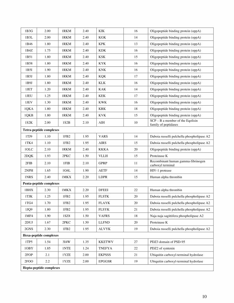
Table 1. The 44 protein-peptide complexes used as test cases in this study, grouped by the length of the peptide ligand

Results and discussions

We generated 1,500 docked structures for each test case of the benchmarking dataset. In

this discussion, we specifically pick two structures from these. The first structure we identify for

our analysis is what we call ‘the best sampled structure’. For each test case, we consider the

peptide structure in the respective holo protein-peptide complex as the native structure. The

1,500 peptide-protein complex structures generated using MOLS were each superimposed on the

native structure without further changing the orientation. The RMSD was calculated on the

peptide backbone alone. This procedure measures the differences not only in the structure of the

peptide, but also in its pose with respect to the protein. We identify the best sampled structure as

one in which the peptide has the lowest backbone RMSD with respect to the native structure.

PDB ID

Peptide Sequence

Native energy

Lowest Energya Best Sampledd Rankinge

(%) RMSDb

(Å) Energy

(no unit) RDEc

(%) RMSD

(Å) Energy

(no unit) RDE (%)

8GCH GAW -870.81 1.69 -949.43 53.11 1.62 -859.77 46.78 4.20 1A30 EDL -886.99 5.83 -792.56 75.09 1.10 -713.90 57.56 11.50 1B32 KMK -1481.97 5.55 -1032.87 74.00 1.72 -896.85 60.14 35.70 1B05 KCK -1395.40 5.84 -1029.37 72.72 2.09 -924.41 60.37 12.20 1B3F KHK -1464.94 3.03 -1077.60 64.00 1.79 -968.99 58.01 12.60 1B3L KGK -1254.63 6.00 -988.15 72.58 1.81 -816.13 61.97 61.30 1B3G KIK -1394.79 3.66 -1041.50 66.30 1.98 -919.84 57.18 9.60

12

1B46 KPK -1428.67 3.39 -944.46 62.89 2.05 -661.75 62.33 69.40 1B4Z KDK -1447.42 6.00 -1053.49 74.89 1.96 -881.66 63.54 49.80 1B51 KSK -1423.22 6.53 -1080.75 74.21 1.89 -890.99 59.53 39.30 1B58 KYK -1516.95 5.50 -1089.65 70.73 1.88 -1014.91 59.88 9.07 1B5I KNK -1465.83 6.43 -1076.80 74.70 2.06 -850.59 62.69 71.70 1B5J KQK -1504.96 4.01 -1066.40 70.61 1.97 -520.93 64.44 97.90 1B9J KLK -1441.99 6.44 -1047.52 75.09 1.95 -928.64 62.27 21.30 1JET KAK -1323.79 4.70 -1033.05 66.73 1.87 -798.73 61.86 77.90 1JEU KEK -1444.22 4.68 -1062.08 74.31 1.92 -841.29 63.00 69.00 1JEV KWK -1454.60 6.43 -1131.75 72.68 1.89 -1003.52 60.73 15.90 1QKA KRK -1551.75 6.29 -1062.55 72.74 2.00 -813.83 68.90 73.80 1QKB KVK -1459.48 6.49 -1071.12 73.81 1.80 -880.55 59.31 52.00 1S2K AIH -600.46 5.80 -715.40 72.11 1.50 -608.98 61.31 15.70 1TK4 AIRS -774.76 5.78 -682.09 68.73 2.21 -543.39 63.39 2.80 1TJ9 VARS -571.31 6.10 -658.96 72.60 1.46 -463.23 56.60 55.90 2FIB GPRP -717.24 6.48 -789.57 75.29 1.63 -615.93 56.46 30.70

2DQK VLLH -171.34 5.26 -957.89 67.21 1.99 -796.92 61.78 49.70 2NPH AETF -827.63 5.52 -906.61 71.65 1.54 -839.45 51.93 1.30 1OLC KKKA -1560.03 2.74 -1145.00 69.82 2.10 -760.29 76.36 82.40 1NRS LDPR -822.17 4.92 -489.16 71.52 1.63 -455.34 57.42 0.73 2DUJ LLFND -1256.21 8.54 -1058.33 73.76 3.21 -1026.52 59.94 0.50 1MF4 VAFRS -745.03 5.68 -1289.01 70.35 2.28 -1110.16 66.52 12.73 1TJK FLSTK -700.96 8.23 -447.40 79.02 2.71 -224.57 65.98 49.53 1TG4 FLAYK 4109.31f 4.67 -473.24 70.19 2.51 -206.20 61.28 49.33 1JQ9 FLSYK -928.87 1.92 -567.13 62.21 1.64 -399.28 62.75 2.47 2GNS ALVYK 35.04 9.58 -867.40 76.57 1.93 -202.37 60.00 31.93 1BHX DFEEI -659.31 7.98 -440.13 78.97 2.01 -230.46 59.05 27.40 1OBY TNEFYA -1412.04 8.69 -878.12 78.48 5.23 -475.11 73.09 94.30 1TP5 KKETWV -1032.59 2.81 -821.69 64.36 1.95 -755.57 60.50 0.40 2FOO EPGGSR -905.22 3.30 -1258.99 64.21 1.80 -1063.24 54.52 25.60 2FOP EKPSSS -943.37 3.81 -1345.65 66.61 2.41 -1212.60 62.88 10.87 1KY6 FSDPWGG -1037.78 7.08 -1036.66 66.91 2.93 -977.11 63.98 1.07 1U8I ELDKWAN -1045.50 9.83 -1080.34 79.56 2.15 -982.20 61.35 1.80 1P7V PAPFAAA 8705.57g 7.15 -902.98 73.05 2.55 -738.16 57.56 10.40 2FOJ GARAHSS -1111.47 8.90 -1756.19 74.41 2.78 -1553.74 61.06 42.40 1P7W PAPFASA -441.29 4.97 -851.07 71.58 2.65 -781.21 57.94 2.40 2HD4 GDEQGENK -909.21 11.20 -1179.33 83.03 3.19 -815.53 66.60 79.73

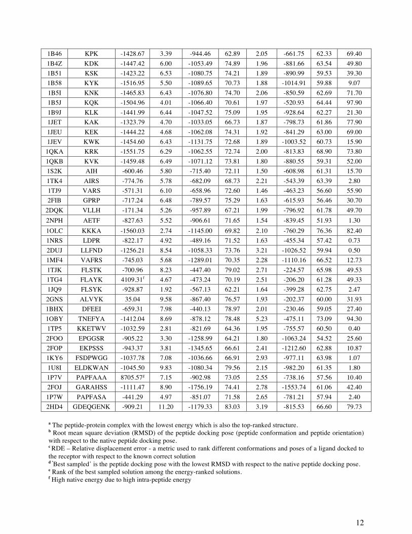
a The peptide-protein complex with the lowest energy which is also the top-ranked structure. b Root mean square deviation (RMSD) of the peptide docking pose (peptide conformation and peptide orientation) with respect to the native peptide docking pose. c RDE – Relative displacement error - a metric used to rank different conformations and poses of a ligand docked to the receptor with respect to the known correct solution

d ‘Best sampled’ is the peptide docking pose with the lowest RMSD with respect to the native peptide docking pose. e Rank of the best sampled solution among the energy-ranked solutions. f High native energy due to high intra-peptide energy

13

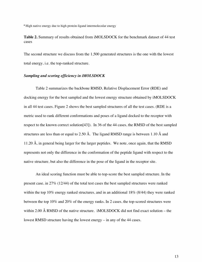
g High native energy due to high protein-ligand intermolecular energy

Table 2. Summary of results obtained from iMOLSDOCK for the benchmark dataset of 44 test cases

The second structure we discuss from the 1,500 generated structures is the one with the lowest

total energy, i.e. the top-ranked structure.

Sampling and scoring efficiency in iMOLSDOCK

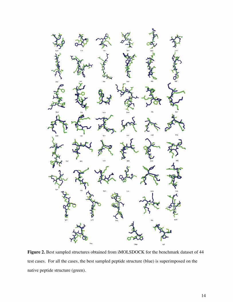
Table 2 summarizes the backbone RMSD, Relative Displacement Error (RDE) and

docking energy for the best sampled and the lowest energy structure obtained by iMOLSDOCK

in all 44 test cases. Figure 2 shows the best sampled structures of all the test cases. (RDE is a

metric used to rank different conformations and poses of a ligand docked to the receptor with

respect to the known correct solution[43]). In 36 of the 44 cases, the RMSD of the best sampled

structures are less than or equal to 2.50 Å. The ligand RMSD range is between 1.10 Å and

11.20 Å, in general being larger for the larger peptides. We note, once again, that the RMSD

represents not only the difference in the conformation of the peptide ligand with respect to the

native structure, but also the difference in the pose of the ligand in the receptor site.

An ideal scoring function must be able to top-score the best sampled structure. In the

present case, in 27% (12/44) of the total test cases the best sampled structures were ranked

within the top 10% energy ranked structures, and in an additional 18% (8/44) they were ranked

between the top 10% and 20% of the energy ranks. In 2 cases, the top-scored structures were

within 2.00 Å RMSD of the native structure. iMOLSDOCK did not find exact solution – the

lowest RMSD structure having the lowest energy – in any of the 44 cases.

14

Figure 2. Best sampled structures obtained from iMOLSDOCK for the benchmark dataset of 44

test cases. For all the cases, the best sampled peptide structure (blue) is superimposed on the

native peptide structure (green).

15

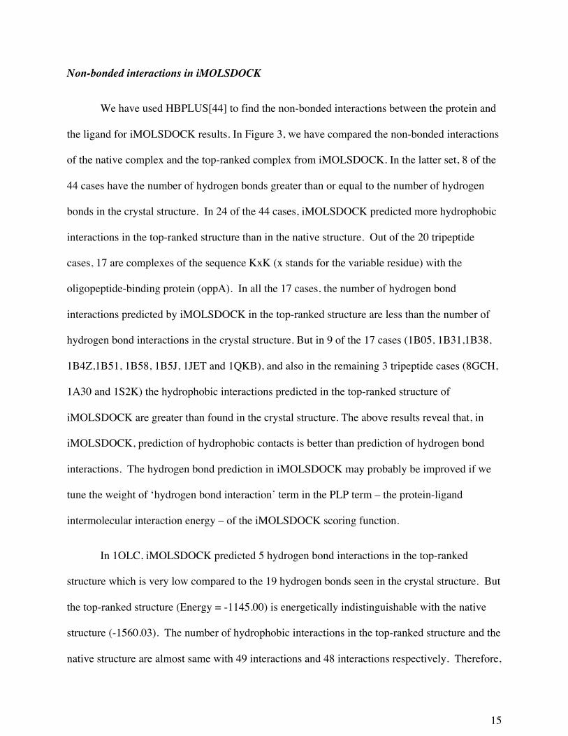
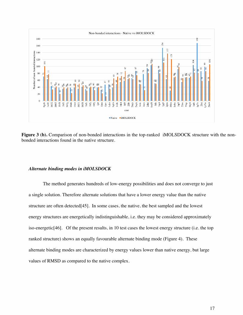
Non-bonded interactions in iMOLSDOCK

We have used HBPLUS[44] to find the non-bonded interactions between the protein and

the ligand for iMOLSDOCK results. In Figure 3, we have compared the non-bonded interactions

of the native complex and the top-ranked complex from iMOLSDOCK. In the latter set, 8 of the

44 cases have the number of hydrogen bonds greater than or equal to the number of hydrogen

bonds in the crystal structure. In 24 of the 44 cases, iMOLSDOCK predicted more hydrophobic

interactions in the top-ranked structure than in the native structure. Out of the 20 tripeptide

cases, 17 are complexes of the sequence KxK (x stands for the variable residue) with the

oligopeptide-binding protein (oppA). In all the 17 cases, the number of hydrogen bond

interactions predicted by iMOLSDOCK in the top-ranked structure are less than the number of

hydrogen bond interactions in the crystal structure. But in 9 of the 17 cases (1B05, 1B31,1B38,

1B4Z,1B51, 1B58, 1B5J, 1JET and 1QKB), and also in the remaining 3 tripeptide cases (8GCH,

1A30 and 1S2K) the hydrophobic interactions predicted in the top-ranked structure of

iMOLSDOCK are greater than found in the crystal structure. The above results reveal that, in

iMOLSDOCK, prediction of hydrophobic contacts is better than prediction of hydrogen bond

interactions. The hydrogen bond prediction in iMOLSDOCK may probably be improved if we

tune the weight of ‘hydrogen bond interaction’ term in the PLP term – the protein-ligand

intermolecular interaction energy – of the iMOLSDOCK scoring function.

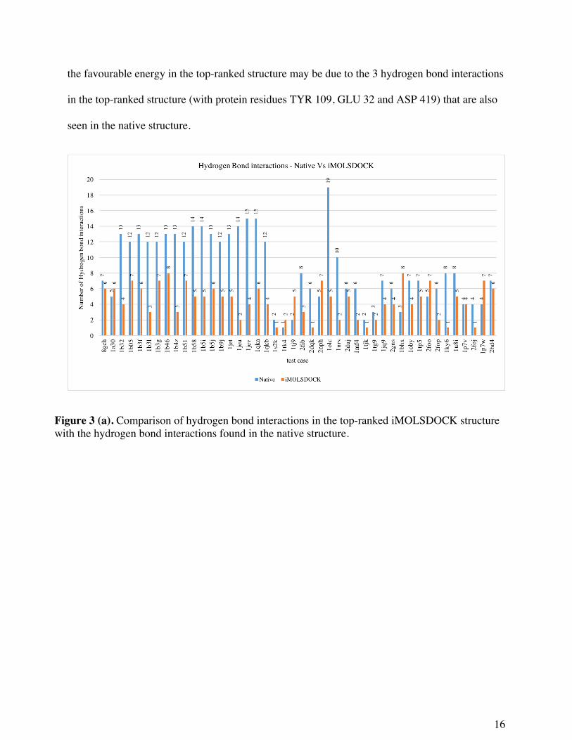
In 1OLC, iMOLSDOCK predicted 5 hydrogen bond interactions in the top-ranked

structure which is very low compared to the 19 hydrogen bonds seen in the crystal structure. But

the top-ranked structure (Energy = -1145.00) is energetically indistinguishable with the native

structure (-1560.03). The number of hydrophobic interactions in the top-ranked structure and the

native structure are almost same with 49 interactions and 48 interactions respectively. Therefore,

16

the favourable energy in the top-ranked structure may be due to the 3 hydrogen bond interactions

in the top-ranked structure (with protein residues TYR 109, GLU 32 and ASP 419) that are also

seen in the native structure.

Figure 3 (a). Comparison of hydrogen bond interactions in the top-ranked iMOLSDOCK structure with the hydrogen bond interactions found in the native structure.

17

Figure 3 (b). Comparison of non-bonded interactions in the top-ranked iMOLSDOCK structure with the non-bonded interactions found in the native structure.

Alternate binding modes in iMOLSDOCK

The method generates hundreds of low-energy possibilities and does not converge to just

a single solution. Therefore alternate solutions that have a lower energy value than the native

structure are often detected[45]. In some cases, the native, the best sampled and the lowest

energy structures are energetically indistinguishable, i.e. they may be considered approximately

iso-energetic[46]. Of the present results, in 10 test cases the lowest energy structure (i.e. the top

ranked structure) shows an equally favourable alternate binding mode (Figure 4). These

alternate binding modes are characterized by energy values lower than native energy, but large

values of RMSD as compared to the native complex.

18

Figure 4. Alternate binding modes predicted by iMOLSDOCK top-ranked structures. The top-ranked structure of iMOLSDOCK is shown in blue and the native structure is shown in green. The native energy in 1P7V is high due to short contacts between the peptide and the protein.

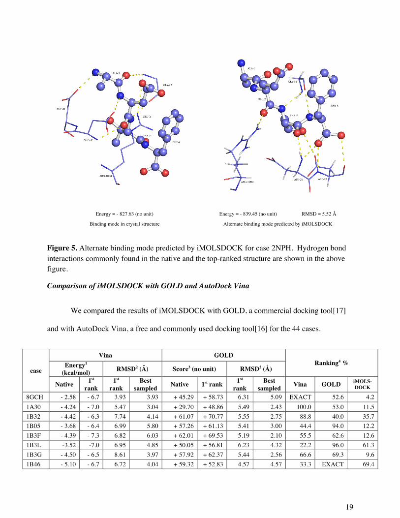
Of particular note is the structure 2NPH. In this test case, the top-ranked structure has a

larger number of hydrogen bond interactions than seen in the native complex. However, the

RMSD of the top ranked structure with respect to the crystal structure is 5.52 Å. In 2NPH the

top ranked structure predicted more hydrogen bond interactions (hydrogen bonds = 7) than the

native structure (hydrogen bonds = 5). Figure 5 shows the hydrogen bond interactions of 2NPH

common to the native structure and the top ranked structure.

19

Energy = - 827.63 (no unit) Energy = - 839.45 (no unit) RMSD = 5.52 Å

Binding mode in crystal structure Alternate binding mode predicted by iMOLSDOCK

Figure 5. Alternate binding mode predicted by iMOLSDOCK for case 2NPH. Hydrogen bond interactions commonly found in the native and the top-ranked structure are shown in the above figure.

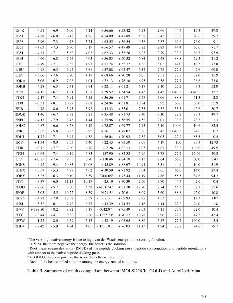
Comparison of iMOLSDOCK with GOLD and AutoDock Vina

We compared the results of iMOLSDOCK with GOLD, a commercial docking tool[17]

and with AutoDock Vina, a free and commonly used docking tool[16] for the 44 cases.

case

Vina GOLD Ranking4 % Energy1

(kcal/mol) RMSD2 (Å) Score3 (no unit) RMSD2 (Å)

Native 1st rank

1st rank

Best sampled Native 1st rank 1st

rank Best

sampled Vina GOLD iMOLS- DOCK

8GCH - 2.58 - 6.7 3.93 3.93 + 45.29 + 58.73 6.31 5.09 EXACT 52.6 4.2 1A30 - 4.24 - 7.0 5.47 3.04 + 29.70 + 48.86 5.49 2.43 100.0 53.0 11.5 1B32 - 4.42 - 6.3 7.74 4.14 + 61.07 + 70.77 5.55 2.75 88.8 40.0 35.7 1B05 - 3.68 - 6.4 6.99 5.80 + 57.26 + 61.13 5.41 3.00 44.4 94.0 12.2 1B3F - 4.39 - 7.3 6.82 6.03 + 62.01 + 69.53 5.19 2.10 55.5 62.6 12.6 1B3L -3.52 -7.0 6.95 4.85 + 50.05 + 56.81 6.23 4.32 22.2 96.0 61.3 1B3G - 4.50 - 6.5 8.61 3.97 + 57.92 + 62.37 5.44 2.56 66.6 69.3 9.6 1B46 - 5.10 - 6.7 6.72 4.04 + 59.32 + 52.83 4.57 4.57 33.3 EXACT 69.4

20

1B4Z - 4.51 - 6.9 6.00 5.24 + 56.66 + 53.42 5.33 2.66 44.4 15.3 49.8 1B51 - 4.28 - 6.8 6.48 4.96 + 54.09 + 47.89 5.38 2.42 33.3 90.6 39.2 1B58 - 5.96 - 7.3 4.78 3.74 + 63.55 + 56.54 6.38 2.87 66.6 76.0 9.1 1B5I - 4.63 - 7.3 6.90 5.19 + 56.57 + 47.49 5.82 2.83 44.4 66.6 71.7 1B5J - 4.81 - 7.1 5.62 4.03 + 62.33 + 53.28 6.23 2.79 33.3 89.3 97.9 1B9J - 4.66 - 6.8 7.55 4.03 + 56.03 + 50.32 6.84 2.48 88.8 29.3 21.2 1JET - 4.79 - 7.1 7.32 4.97 + 51.74 + 55.72 4.36 3.02 44.0 19.3 77.8 1JEU - 4.98 - 6.5 6.92 5.81 + 57.08 + 62.47 6.32 2.78 77.7 2.6 69.0 1JEV - 5.66 - 7.6 7.70 4.17 + 68.66 + 70.28 6.05 2.51 88.8 32.0 15.9 1QKA - 5.06 - 6.9 7.08 4.04 + 72.13 + 76.10 6.95 2.58 77.7 26.6 73.8 1QKB - 4.28 - 6.5 7.41 3.94 + 22.11 + 61.21 6.17 2.10 22.2 3.3 52.0 1S2K - 4.12 - 6.7 1.21 1.21 + 29.52 + 54.54 4.45 4.45 EXACT EXACT 15.7 1TK4 - 2.17 - 7.4 6.92 6.55 + 36.56 + 61.71 7.47 5.06 88.8 51.3 2.8 1TJ9 - 0.31 - 8.1 10.27 9.68 + 24.94 + 31.81 10.94 6.92 66.6 66.0 55.9 2FIB - 4.78 - 8.6 5.95 3.92 + 43.33 + 53.01 7.33 5.52 33.3 42.6 30.7 2DQK - 1.46 - 6.7 8.32 3.21 + 35.48 + 71.73 7.40 3.10 22.2 89.3 49.7 2NPH - 4.13 - 7.9 3.46 1.44 + 35.96 + 56.55 4.52 2.01 33.3 23.3 1.3 1OLC - 4.87 - 6.6 8.58 3.19 + 75.87 + 69.77 7.43 5.16 100.0 10.6 82.4 1NRS - 3.62 - 5.8 6.95 6.95 + 56.11 + 79.07 8.36 3.45 EXACT 24.6 0.7 2DUJ - 1.72 - 7.1 5.97 4.38 + 26.04 + 70.92 7.32 5.03 22.2 83.3 0.5 1MF4 + 1.34 - 8.0 8.53 6.40 - 22.43 + 73.59 8.09 4.19 100 83.3 12.73 1TJK - 0.72 - 7.7 7.60 6.76 + 7.28 + 82.13 7.05 4.81 88.8 16.66 49.5 1TG4 + 0.64 - 7.4 9.19 5.83 - 157.90 + 82.33 5.96 3.78 77.7 12.66 49.3 1JQ9 + 0.85 - 7.4 9.95 6.70 - 110.46 + 84.10 9.13 2.64 66.6 60.0 2.47 2GNS - 4.42 - 9.4 10.83 10.06 + 45.89 + 88.67 10.94 3.51 44.4 10.0 31.9 1BHX - 3.57 - 5.3 4.77 4.62 + 30.59 + 71.92 8.64 5.65 66.6 14.0 27.4 1OBY - 5.25 - 6.3 9.10 8.39 - 2700.65c + 73.44 11.19 7.86 55.5 34.6 94.2 1TP5 - 3.37 - 6.0 11.13 10.17 - 25.19 + 70.39 7.60 5.70 44.4 2.6 0.4 2FOO - 2.66 - 5.7 7.00 5.58 - 4131.54 c + 81.78 12.70 2.74 55.5 32.7 25.6 2FOP - 3.03 - 5.5 10.22 8.39 - 9624.5 c + 70.61 8.09 5.60 88.8 92.0 10.8 1KY6 - 4.72 - 7.8 12.32 8.38 - 1332.56 c + 69.93 7.92 4.33 33.3 17.3 1.07 1U8I - 3.52 - 6.1 7.42 6.77 + 43.39 + 74.52 7.16 4.14 22.2 24.0 1.8 1P7V + 598.80 - 8.2 8.82 5.17 - 6042.07c + 75.49 8.03 4.11 77.7 72.0 10.4 2FOJ - 3.44 - 4.1 9.36 6.20 - 1327.70c + 70.12 10.78 2.96 22.2 47.3 42.4 1P7W - 1.52 - 8.0 6.59 5.17 + 42.19 + 68.65 8.86 5.47 77.7 100.0 2.4 2HD4 - 2.42 - 5.9 4.74 4.05 - 1351.01c + 76.03 11.13 4.24 88.8 24.6 79.7

c The very high native energy is due to high van der Waals energy in the scoring function. 1 In Vina, the more negative the energy, the better is the solution. 2 Root mean square deviation (RMSD) of the peptide docking pose (peptide conformation and peptide orientation) with respect to the native peptide docking pose. 3 In GOLD, the more positive the score the better is the solution. 4 Rank of the best sampled solution among the energy-ranked solutions. Table 3. Summary of results comparison between iMOLSDOCK, GOLD and AutoDock Vina

21

GOLD is a GA-based docking tool. The parameters of the fitness function were fixed to

their default values. A total of 150 GA runs were performed for each test case. We set the

docking speed to ‘slow (most accurate)’ which equated to 100,000 operations. The rest of the

options were set to ‘automatic’.

AutoDock Vina is an open-source program for molecular docking[16]. It uses Iterated

Local Search global optimizer algorithm where a succession of steps are taken, each consisting

of a mutation and a local optimization. Each step is accepted or rejected according to the

Metropolis criterion. The grid size for the search space was set to the optimum size mentioned by

the authors[16], to accommodate the extended conformation of the peptide ligand inside the grid

box. The centre of the grid box was set to the centre of the peptide. All other settings

(exhaustiveness, number of modes, etc.) have been set to the default values. The input peptide

structure for both GOLD and Vina was the extended structure built using the MOLS 2.0 -

peptide modeling tool[30]. In iMOLSDOCK, the amino acid sequence of the peptide ligand is

given as input; the extended structure of the peptide is automatically built using the BUILDER

routine of the iMOLSDOCK algorithm. Table 3 summarises the backbone RMSD of the top-

ranked structures, RMSD of the best sampled structures and energy of the top-ranked structures

of GOLD and Vina. Table 3 also shows the ranking efficiency of Vina, GOLD and

iMOLSDOCK.

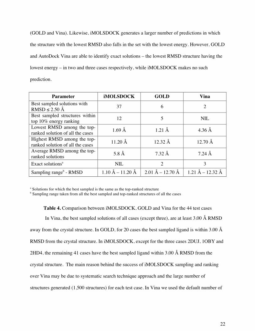
Table 4 shows a comparison of the results from iMOLSDOCK, GOLD and Vina. The

number of cases in which the prediction with lowest RMSD with respect to the native complex

(i.e. the best sampled structure has the RMSD value less than 2.50 Å) is the greatest in the case

of iMOLSDOCK. Clearly this program, iMOLSDOCK, is able to arrive at docked structures

that are close to the crystal structure in a larger number of cases than the other two algorithms

22

(GOLD and Vina). Likewise, iMOLSDOCK generates a larger number of predictions in which

the structure with the lowest RMSD also falls in the set with the lowest energy. However, GOLD

and AutoDock Vina are able to identify exact solutions – the lowest RMSD structure having the

lowest energy – in two and three cases respectively, while iMOLSDOCK makes no such

prediction.

Parameter iMOLSDOCK GOLD Vina Best sampled solutions with RMSD ≤ 2.50 Å 37 6 2

Best sampled structures within top 10% energy ranking 12 5 NIL

Lowest RMSD among the top-ranked solution of all the cases 1.69 Å 1.21 Å 4.36 Å

Highest RMSD among the top-ranked solution of all the cases 11.20 Å 12.32 Å 12.70 Å

Average RMSD among the top-ranked solutions 5.8 Å 7.32 Å 7.24 Å

Exact solutionsa NIL 2 3 Sampling rangeb - RMSD 1.10 Å – 11.20 Å 2.01 Å – 12.70 Å 1.21 Å – 12.32 Å a Solutions for which the best sampled is the same as the top-ranked structure b Sampling range taken from all the best sampled and top-ranked structures of all the cases

Table 4. Comparison between iMOLSDOCK, GOLD and Vina for the 44 test cases

In Vina, the best sampled solutions of all cases (except three), are at least 3.00 Å RMSD

away from the crystal structure. In GOLD, for 20 cases the best sampled ligand is within 3.00 Å

RMSD from the crystal structure. In iMOLSDOCK, except for the three cases 2DUJ, 1OBY and

2HD4, the remaining 41 cases have the best sampled ligand within 3.00 Å RMSD from the

crystal structure. The main reason behind the success of iMOLSDOCK sampling and ranking

over Vina may be due to systematic search technique approach and the large number of

structures generated (1,500 structures) for each test case. In Vina we used the default number of

23

binding modes (9 binding modes) and exhaustiveness. As part of the testing, for all the cases we

tried increasing the number of binding modes (num_modes) and the exhaustiveness but the

results were similar to that obtained with the default num_modes and exhaustiveness.

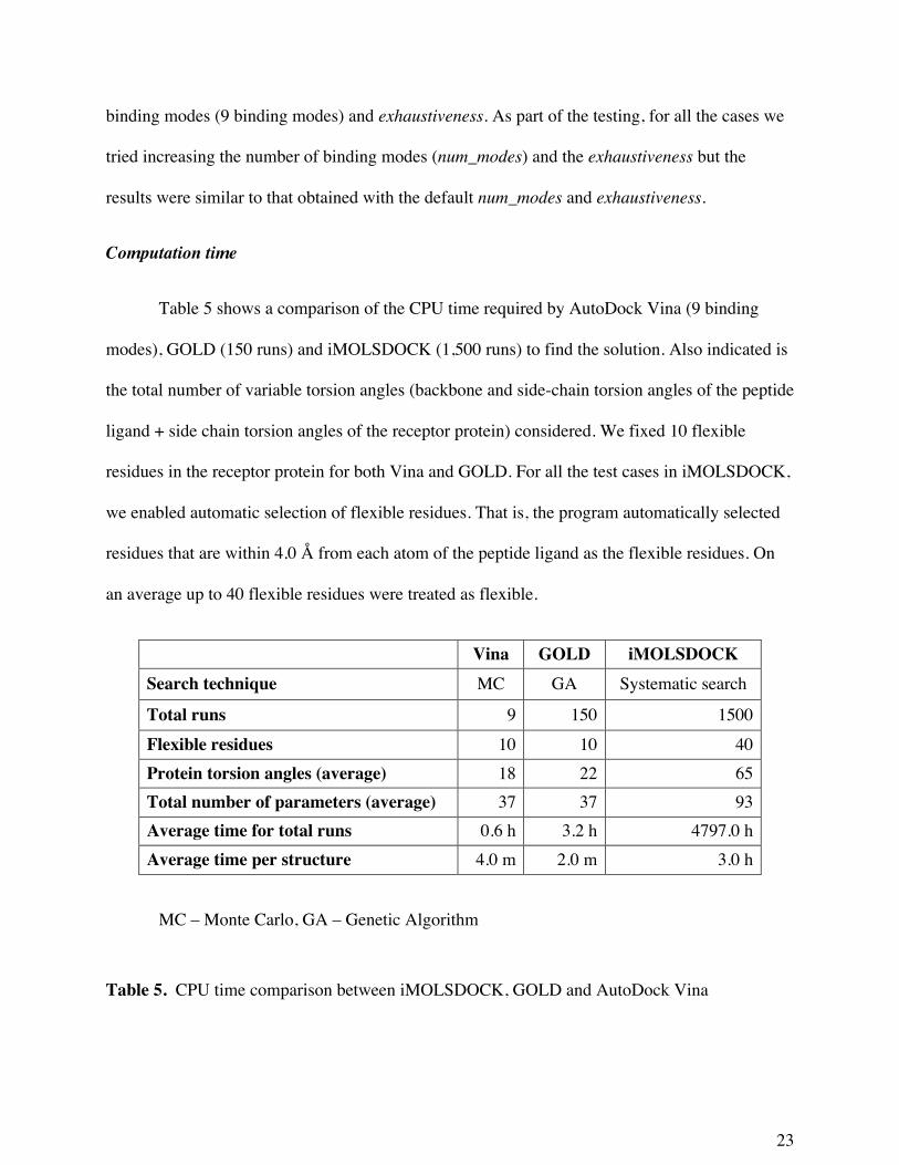
Computation time

Table 5 shows a comparison of the CPU time required by AutoDock Vina (9 binding

modes), GOLD (150 runs) and iMOLSDOCK (1,500 runs) to find the solution. Also indicated is

the total number of variable torsion angles (backbone and side-chain torsion angles of the peptide

ligand + side chain torsion angles of the receptor protein) considered. We fixed 10 flexible

residues in the receptor protein for both Vina and GOLD. For all the test cases in iMOLSDOCK,

we enabled automatic selection of flexible residues. That is, the program automatically selected

residues that are within 4.0 Å from each atom of the peptide ligand as the flexible residues. On

an average up to 40 flexible residues were treated as flexible.

Vina GOLD iMOLSDOCK Search technique MC GA Systematic search

Total runs 9 150 1500 Flexible residues 10 10 40 Protein torsion angles (average) 18 22 65 Total number of parameters (average) 37 37 93 Average time for total runs 0.6 h 3.2 h 4797.0 h Average time per structure 4.0 m 2.0 m 3.0 h

MC – Monte Carlo, GA – Genetic Algorithm

Table 5. CPU time comparison between iMOLSDOCK, GOLD and AutoDock Vina

24

The average CPU time required for one run is 4 m for AutoDock Vina, 2 m for GOLD

and 3 h for iMOLSDOCK. The CPU time of iMOLSDOCK is a function of number of peptide

torsion angles, number of protein torsion angles and number of protein atoms in the docking

space.

Conclusions

We have enhanced the capability of the iMOLSDOCK docking algorithm by

incorporating ‘induced-fit’ side-chain receptor flexibility. Test runs using 44 peptide-protein

complexes from the PDB show that the program performs well. Comparison using the same test

cases with GOLD and AutoDock Vina, shows that iMOLSDOCK outperforms these two

commonly used programs, though it consumes an order of magnitude more computer time. It

may be noted however, that not only is the search space vastly greater in iMOLSDOCK than in

the other two, incorporating, as it does, a larger number of flexible residues, but also the search is

systematic and not stochastic. An added advantage of the iMOLSDOCK algorithm, as pointed

out earlier[6,7] is its ability to identify alternate binding modes. This paper reports

iMOLSDOCK as demonstrated and tested for peptide ligands. However, it is straightforward to

extend the algorithm it to other drug-like ligands.

CONFLICT OF INTEREST

The authors declare no conflict of interest.

ACKNOWLEDGMENT

We thank the Department of Science and Technology, Government of India, for financial support.

We also thank the University Grants Commission for support under the CAS program.

25

REFERENCES

[1] I.D. Kuntz, J.M. Blaney, S.J. Oatley, R. Langridge, T.E. Ferrin, A geometric approach to macromolecule-ligand interactions., J. Mol. Biol. 161 (1982) 269–288.

[2] R.L. DesJarlais, R.P. Sheridan, G.L. Seibel, J.S. Dixon, I.D. Kuntz, R. Venkataraghavan, Using shape complementarity as an initial screen in designing ligands for a receptor binding site of known three-dimensional structure., J. Med. Chem. 31 (1988) 722–729.

[3] R.L. DesJarlais, R.P. Sheridan, J.S. Dixon, I.D. Kuntz, R. Venkataraghavan, Docking flexible ligands to macromolecular receptors by molecular shape., J. Med. Chem. 29 (1986) 2149–2153.

[4] I.D. Kuntz, Structure-based strategies for drug design and discovery., Science. 257 (1992) 1078–1082.

[5] G.M. Morris, D.S. Goodsell, R.S. Halliday, R. Huey, W.E. Hart, R.K. Belew, A.J. Olson, Automated docking using a Lamarckian genetic algorithm and an empirical binding free energy function, J. Comput. Chem. 19 (1998) 1639–1662.

[6] P. Arun Prasad, N. Gautham, A new peptide docking strategy using a mean field technique with mutually orthogonal Latin square sampling, J. Comput. Aided Mol. Des. 22 (2008) 815–829.

[7] S.N. Viji, P.A. Prasad, N. Gautham, Protein- Ligand Docking Using Mutually Orthogonal Latin Squares (MOLSDOCK), J. Chem. Inf. Model. 49 (2009) 2687–2694.

[8] K. Vengadesan, N. Gautham, Enhanced sampling of the molecular potential energy surface using mutually orthogonal Latin squares: Application to peptide structures, Biophys. J. 84 (2003) 2897.

[9] Ito K., Encyclopedic Dictionary of Mathematics, MIT Press, Cambridge, Massachussets, 1987.

[10] P. Koehl, M. Delarue, Mean-field minimization methods for biological macromolecules, Curr. Opin. Struct. Biol. 6 (1996) 222–226. doi:http://dx.doi.org/10.1016/S0959-440X(96)80078-9.

[11] D.E. Koshland, Application of a Theory of Enzyme Specificity to Protein Synthesis, Proc. Natl. Acad. Sci. U. S. A. 44 (1958) 98–104.

[12] J. Monod, J.-P. Changeux, F. Jacob, Allosteric proteins and cellular control systems, J. Mol. Biol. 6 (1963) 306–329. doi:http://dx.doi.org/10.1016/S0022-2836(63)80091-1.

[13] J. Monod, J. Wyman, J.-P. Changeux, On the nature of allosteric transitions: A plausible model, J. Mol. Biol. 12 (1965) 88–118. doi:http://dx.doi.org/10.1016/S0022-2836(65)80285-6.

[14] M.I. Zavodszky, Side-chain flexibility in protein-ligand binding: The minimal rotation hypothesis, Protein Sci. 14 (2005) 1104–1114. doi:10.1110/ps.041153605.

[15] R. Najmanovich, J. Kuttner, V. Sobolev, M. Edelman, Side-chain flexibility in proteins upon ligand binding, Proteins Struct. Funct. Bioinforma. 39 (2000) 261–268. doi:10.1002/(SICI)1097-0134(20000515)39:3<261::AID-PROT90>3.0.CO;2-4.

[16] O. Trott, A.J. Olson, AutoDock Vina: Improving the speed and accuracy of docking with a new scoring function, efficient optimization, and multithreading, J. Comput. Chem. 31 (2010) 455–461. doi:10.1002/jcc.21334.

[17] G. Jones, P. Willett, R.C. Glen, A.R. Leach, R. Taylor, Development and validation of a genetic algorithm for flexible docking., J. Mol. Biol. 267 (1997) 727–748. doi:10.1006/jmbi.1996.0897.

26

[18] W. Sherman, H.S. Beard, R. Farid, Use of an induced fit receptor structure in virtual screening., Chem. Biol. Drug Des. 67 (2006) 83–84. doi:10.1111/j.1747-0285.2005.00327.x.

[19] J. Meiler, D. Baker, ROSETTALIGAND: Protein–small molecule docking with full side-chain flexibility, Proteins Struct. Funct. Bioinforma. 65 (2006) 538–548. doi:10.1002/prot.21086.

[20] R. Das, D. Baker, Macromolecular modeling with rosetta., Annu. Rev. Biochem. 77 (2008) 363–382. doi:10.1146/annurev.biochem.77.062906.171838.

[21] I.W. Davis, D. Baker, RosettaLigand docking with full ligand and receptor flexibility, J. Mol. Biol. 385 (2009) 381–392.

[22] G. Lemmon, J. Meiler, Rosetta Ligand docking with flexible XML protocols., Methods Mol. Biol. Clifton NJ. 819 (2012) 143–155. doi:10.1007/978-1-61779-465-0_10.

[23] S.N. Viji, N. Balaji, N. Gautham, Molecular docking studies of protein-nucleotide complexes using MOLSDOCK (mutually orthogonal Latin squares DOCK), J. Mol. Model. (2012) 1–18.

[24] K. Vengadesan, Sampling the Molecular Potential Energy Surface Using Mutually Orthogonal Latin Squares and Application to Peptide Structures, Dissertation, University of Madras, 2004.

[25] K. Vengadesan, N. Gautham, Conformational studies on enkephalins using the MOLS technique, Biopolymers. 74 (2004) 476–494.

[26] K. Vengadesan, T. Anbupalam, N. Gautham, An application of experimental design using mutually orthogonal Latin squares in conformational studies of peptides, Biochem. Biophys. Res. Commun. 316 (2004) 731–737.

[27] V. Kanagasabai, J. Arunachalam, P. Arun Prasad, N. Gautham, Exploring the conformational space of protein loops using a mean field technique with MOLS sampling, Proteins Struct. Funct. Bioinforma. 67 (2007) 908–921.

[28] C.L. Liu, Introduction to Combinatorial Mathematics, McGraw-Hill Book Co, New York, 1968.

[29] K. Vengadesan, N. Gautham, Energy landscape of Met-enkephalin and Leu-enkephalin drawn using mutually orthogonal Latin squares sampling, J. Phys. Chem. B. 108 (2004) 11196–11205.

[30] D. Sam Paul, N. Gautham, MOLS 2.0: software package for peptide modeling and protein–ligand docking, J. Mol. Model. 22 (2016) 1–9. doi:10.1007/s00894-016-3106-x.

[31] V. Le Guilloux, P. Schmidtke, P. Tuffery, Fpocket: an open source platform for ligand pocket detection, BMC Bioinformatics. 10 (2009) 168.

[32] M.E. Fraser, N.C.J. Strynadka, P.A. Bartlett, J.E. Hanson, M.N.G. James, Crystallographic analysis of transition-state mimics bound to penicillopepsin: phosphorus-containing peptide analogs, Biochemistry (Mosc.). 31 (1992) 5201–5214. doi:10.1021/bi00137a016.

[33] H.J. Hecht, M. Szardenings, J. Collins, D. Schomburg, Three-dimensional structure of a recombinant variant of human pancreatic secretory trypsin inhibitor (Kazal type)., J. Mol. Biol. 225 (1992) 1095–1103.

[34] M. Ikura, G.M. Clore, A.M. Gronenborn, G. Zhu, C.B. Klee, A. Bax, Solution structure of a calmodulin-target peptide complex by multidimensional NMR., Science. 256 (1992) 632–638.

[35] A.M. Lesk, C. Chothia, Elbow motion in the immunoglobulins involves a molecular ball-and-socket joint., Nature. 335 (1988) 188–190. doi:10.1038/335188a0.

27

[36] B.J. Katzin, E.J. Collins, J.D. Robertus, Structure of ricin A-chain at 2.5 Å, Proteins Struct. Funct. Bioinforma. 10 (1991) 251–259. doi:10.1002/prot.340100309.

[37] Z. Xu, D.A. Bernlohr, L.J. Banaszak, Crystal structure of recombinant murine adipocyte lipid-binding protein., Biochemistry (Mosc.). 31 (1992) 3484–3492.

[38] J. Heringa, P. Argos, Strain in protein structures as viewed through nonrotameric side chains: II. effects upon ligand binding., Proteins. 37 (1999) 44–55.

[39] W.D. Cornell, P. Cieplak, C.I. Bayly, I.R. Gould, K.M. Merz, D.M. Ferguson, D.C. Spellmeyer, T. Fox, J.W. Caldwell, P.A. Kollman, A second generation force field for the simulation of proteins, nucleic acids, and organic molecules, J. Am. Chem. Soc. 117 (1995) 5179–5197.

[40] D.K. Gehlhaar, G.M. Verkhivker, P.A. Rejto, C.J. Sherman, D.R. Fogel, L.J. Fogel, S.T. Freer, Molecular recognition of the inhibitor AG-1343 by HIV-1 protease: conformationally flexible docking by evolutionary programming, Chem. Biol. 2 (1995) 317–324.

[41] M. Feig, J. Karanicolas, C.L. 3rd Brooks, MMTSB Tool Set: enhanced sampling and multiscale modeling methods for applications in structural biology., J. Mol. Graph. Model. 22 (2004) 377–395. doi:10.1016/j.jmgm.2003.12.005.

[42] A. Ben-Shimon, M.Y. Niv, AnchorDock: Blind and Flexible Anchor-Driven Peptide Docking, Structure. 23 (2015) 929–940. doi:http://dx.doi.org/10.1016/j.str.2015.03.010.

[43] R.A. Abagyan, M.M. Totrov, Contact area difference (CAD): a robust measure to evaluate accuracy of protein models, J. Mol. Biol. 268 (1997) 678–685.

[44] I.K. McDonald, J.M. Thornton, Satisfying Hydrogen Bonding Potential in Proteins, J. Mol. Biol. 238 (1994) 777–793. doi:http://dx.doi.org/10.1006/jmbi.1994.1334.

[45] R.D. Taylor, P.J. Jewsbury, J.W. Essex, A review of protein-small molecule docking methods, J. Comput. Aided Mol. Des. 16 (2002) 151–166.

[46] R.D. Taylor, P.J. Jewsbury, J.W. Essex, FDS: Flexible ligand and receptor docking with a continuum solvent model and soft-core energy function, J. Comput. Chem. 24 (2003) 1637–1656.