A parameterization of positive definite matrices in terms of ...
27
Linear Algebra and its Applications 372 (2003) 225–251 www.elsevier.com/locate/laa A parameterization of positive definite matrices in terms of partial correlation vines Dorota Kurowicka, Roger Cooke ∗ Delft Institute of Applied Mathematics, Delft University of Technology, Mekelweg 4, Delft 2628 CD, The Netherlands Received 14 April 2000; accepted 31 March 2003 Submitted by R.A. Brualdi Abstract We present a parameterization of the class PD(n) of positive definite n × n matrices using regular vines and partial correlations. Using a bijection from (−1, 1) ( n 2 ) → C(n) (C(n) is the class of n × n correlation matrices) with a clear probabilistic interpretation [Ann. Statist. 30 (4) (2002) 1031], we suggest a new approach to various problems involving positive definite- ness. © 2003 Elsevier Inc. All rights reserved. AMS classification: 60H30; 6209; 62D05; 62H05; 15A48; 15A99 Keywords: Correlation; Tree dependence; Positive definite matrix; Matrix completion 1. Introduction Positive (semi) definiteness is an important property of square matrices. There are algorithms for testing positive definiteness such as the Choleski decomposition or algorithms based on finding eigenvalues of a matrix. We propose to study positive definiteness using partial correlations [4] in conjunction with a new structure which we call a regular vine [1,8]. A symmetric real (n × n) matrix with off-diagonal el- ements in the interval (−1, 1) and with 1’s on the main diagonal is called a proto correlation matrix. For a given n × n proto correlation matrix we consider regular ∗ Corresponding author. E-mail addresses: [email protected] (D. Kurowicka), [email protected] (R. Cooke). 0024-3795/$ - see front matter 2003 Elsevier Inc. All rights reserved. doi:10.1016/S0024-3795(03)00507-X brought to you by CORE View metadata, citation and similar papers at core.ac.uk provided by Elsevier - Publisher Connector
-
Upload
khangminh22 -
Category
Documents
-
view
3 -
download
0
Transcript of A parameterization of positive definite matrices in terms of ...

Linear Algebra and its Applications 372 (2003) 225–251www.elsevier.com/locate/laa
A parameterization of positive definite matricesin terms of partial correlation vines
Dorota Kurowicka, Roger Cooke∗
Delft Institute of Applied Mathematics,Delft University of Technology, Mekelweg 4, Delft 2628 CD, The Netherlands
Received 14 April 2000; accepted 31 March 2003
Submitted by R.A. Brualdi
Abstract
We present a parameterization of the class PD(n) of positive definite n × n matrices using
regular vines and partial correlations. Using a bijection from (−1, 1)(n2) → C(n) (C(n) is the
class of n × n correlation matrices) with a clear probabilistic interpretation [Ann. Statist. 30(4) (2002) 1031], we suggest a new approach to various problems involving positive definite-ness.© 2003 Elsevier Inc. All rights reserved.
AMS classification: 60H30; 6209; 62D05; 62H05; 15A48; 15A99
Keywords: Correlation; Tree dependence; Positive definite matrix; Matrix completion
1. Introduction
Positive (semi) definiteness is an important property of square matrices. Thereare algorithms for testing positive definiteness such as the Choleski decompositionor algorithms based on finding eigenvalues of a matrix. We propose to study positivedefiniteness using partial correlations [4] in conjunction with a new structure whichwe call a regular vine [1,8]. A symmetric real (n × n) matrix with off-diagonal el-ements in the interval (−1, 1) and with 1’s on the main diagonal is called a protocorrelation matrix. For a given n × n proto correlation matrix we consider regular
∗ Corresponding author.E-mail addresses: [email protected] (D. Kurowicka), [email protected] (R. Cooke).
0024-3795/$ - see front matter � 2003 Elsevier Inc. All rights reserved.doi:10.1016/S0024-3795(03)00507-X
brought to you by COREView metadata, citation and similar papers at core.ac.uk
provided by Elsevier - Publisher Connector

226 D. Kurowicka, R. Cooke / Linear Algebra and its Applications 372 (2003) 225–251
vines. A vine is a set of trees such that the edges of the tree Ti are nodes of thetree Ti+1 and all trees have the maximum number of edges. A vine is regular if twoedges of Ti are joined by an edge of Ti+1 only if these edges share a common nodein Ti . A regular vine is called canonical if each tree Ti has a unique node of degreen − i (precise definitions are given in Section 3). In total there are
(n2
)2n−2 partial
correlations. Partial correlations can be assigned to the edges of a regular vine suchthat conditioning and conditioned sets of the vine and partial correlations coincide(see Section 3). There are
(n2
)edges in a regular vine on n elements; hence
(n2
)of
the(n2
)2n−2 partial correlations are selected in this way. It turns out that these partial
correlations are algebraically independent and uniquely determine the correlationmatrix. In fact, a regular vine may be used to construct a bijection from (−1, 1) tothe set of correlation matrices (see Theorem 3.2).
This relationship can be used to specify dependence in high dimensional distribu-tions [2] but also to decide whether a proto correlation matrix is positive definite. Thisalgorithm can be also used to transform a non-positive definite matrix into a positivedefinite matrix. With the new algorithm these alterations have a clear probabilisticinterpretation. This approach can be useful where a high dimensional correlationmatrix should be specified (e.g. dependent Monte Carlo simulations), or when corre-lations are inferred from noisy physical measurements.1 In complex problems manyentries in the correlation matrix may be unspecified, and this partially specified ma-trix must be extended to a positive definite matrix. We present preliminary resultsfor the matrix completion problem using canonical vine partial correlation specifica-tions. In particular, we present effective procedures for deciding whether a partiallyspecified matrix can be extended to a positive definite matrix for certain non-chordalgraphs [3,5,6,9,10].
This paper is organized as follows. In the Section 2 we present definition of partialcorrelations in terms of partial regression coefficients. In Section 3 we introducevines and present definitions and theorems showing relationships between vines andpositive definite matrices. Section 4 contains an algorithm for testing positive defi-niteness of a matrix using the canonical vine. The relationship between the newalgorithm and known matrix theory results is also shown. In Section 5 repairing vio-lation of positive definiteness is given and finally in Section 6 the algorithm solvingthe completion problem for special cases is presented.
2. Partial correlations
Let us consider variables Xi with zero mean and standard deviations σi , i =1, . . . , n. Let the numbers b1n;2,...,n−1, . . . , bn−1;n;1,...,n−2 minimize
E((
Xn − b1n;2,...,n−1X1 − b2n;1,3,...,n−1X2 − · · · − bn−1,n;1,...,n−2Xn−1)2);
1 This arises e.g. in structural mechanics when correlations are inferred from vibration modes.

D. Kurowicka, R. Cooke / Linear Algebra and its Applications 372 (2003) 225–251 227
then the partial correlations are defined as [4]:
ρn,n−1;1,...,n−2 = sgn(bn,n−1;1,...,n−2)(bn,n−1;1,...,n−2bn−1,n;1,...,n−2
)1/2, etc.
Partial correlations can be computed from correlations with the following recursiveformula:
ρn−1,n;1,...,n−2 = ρn,n−1;1,...,n−3 − ρn−2,n;1,...,n−3ρn−2,n−1;1,...,n−3√1 − ρ2
n−2,n;1,...,n−3
√1 − ρ2
n−2,n−1;1,...,n−3
. (1)
All partial correlations can be computed from the correlations by iterating the aboveequation. In general it can be written as follows:
Let X1, . . . , Xn be random variables, and let {i, j, k} be a set of distinct indicesand let C be a (possibly empty) set of indices disjoint from {i, j, k}. The partialcorrelation of Xi and Xj given {Xk,
⋃{Xh | h ∈ C}} is
ρij ;kC = ρij ;C − ρik;Cρjk;C√1 − ρ2
ik;C√
1 − ρ2jk;C
; ρ2ik;C < 1, ρ2
jk;C < 1. (2)
where ρij = ρ(Xi, Xj ). If ρ2ik;C = 1 or ρ2
jk;C = 1, then ρij ;kC is not defined.If X1, . . . , Xn follow a joint normal distribution with variance covariance matrix
of full rank, then partial correlations correspond to conditional correlations. The re-lationship between partial correlations and conditional correlations is studied in [2].
3. Vines
Definition 3.1 (Tree). T = (N, E) is a tree with nodes N and edges E if E is asubset of unordered pairs of N with no cycle and there is a path between each pairof nodes. That is, there does not exist a sequence a1, . . . , ak (k > 2) of elements ofN such that
{a1, a2} ∈ E, . . . , {ak−1, ak} ∈ E, {ak, a1} ∈ E
and for any a, b ∈ N there exists a sequence c2, . . . , ck−1 of elements of N such that
{a, c2} ∈ E, {c2, c3} ∈ E, . . . , {ck−1, b} ∈ E.
Definition 3.2 (Regular vine). V is a regular vine on n elements if
1. V = (T1, . . . , Tn−1);2. T1 is a tree with nodes N1 = {1, . . . , n}, and edges E1; for i = 2, . . . , n − 1, Ti is
a tree with nodes Ni = Ei−1.3. (proximity) for i = 2, . . . , n − 1, {a, b} ∈ Ei , #a�b = 2 where � denotes the
symmetric difference. In other words, if a and b are nodes of Ti connected by

228 D. Kurowicka, R. Cooke / Linear Algebra and its Applications 372 (2003) 225–251
Fig. 1. A regular vine on five elements showing conditioned and conditioning sets.
an edge, where a = {a1, a2}, b = {b1, b2}, then exactly one of the ai equals oneof the bi .
Definition 3.3 (Constraint set).
1. For j ∈ Ei, i � n − 1 the subset Uj (k) of Ei−k = Ni−k+1 defined byUj(k) = {e | ∃ei−(k−1) ∈ ei−(k−2) ∈ · · · ∈ j , e ∈ ei−(k−1)} is called the k-foldunion2 of j ; k = 1, . . . , i.U∗
j = Uj (i) is the complete union of j , that is, the subset of {1, . . . , n} reachablefrom j by the membership relation.If a ∈ N1 then U∗
a = ∅.Uj(1) = {j1, j2} = j .By definition we write Uj (0) = {j}.
2. For i = 1, . . . , n − 1, ei ∈ Ei , if ei = {j, k} then the conditioning set associatedwith ei is
Dei= U∗
j ∩ U∗k
and the conditioned sets associated with ei are
Cei,j = U∗j \ Dei
; Cei,k = U∗k \ Dei
.
3. The constraint set for V is
CV = {Dei, Cei ,j , Cei ,k | ei ∈ Ei; ei = {j, k}, i = 1, . . . , n − 1
}.
Note that for e ∈ E1, the conditioning set is empty. For ei ∈ Ei , i � n − 1, ei ={j, k} we have U∗
ei= U∗
j ∪ U∗k .
We present two examples of a regular vines on five elements with conditioned andconditioning sets (Fig. 1 and Fig. 2). We use the regular vine in Fig. 2 to illustrateDefinition 3.3.
2 The 1-fold union of a set is the set of elements i.e. the set itself, the 2-fold union is the set ofelements of elements, etc.

D. Kurowicka, R. Cooke / Linear Algebra and its Applications 372 (2003) 225–251 229
Fig. 2. A canonical vine on five elements.
We get
T1 = (N1, E1), N1 = {1, 2, . . . , 5}, E1 = {{1, 2}, {1, 3}, {1, 4}, {1, 5}};T2 = (N2, E2), N2 = E1, E2 = {{{1, 2}, {1, 3}}, {{1, 2}, {1, 4}}, {{1, 2}, {1, 5}}};...
The complete union of j = {1, 2} is U∗j = {1, 2} and for k = {1, 3}, U∗
k = {1, 3}.Hence the conditioning set of the edge e = {{1, 2}, {1, 3}} in T2 is De = U∗
j ∩ U∗k =
{1, 2} ∩ {1, 3} = {1}. The conditioned sets are Ce,j = U∗j \ De = {1, 2} \ {1} = {2}
and Ce,k = U∗k \ De = {1, 3} \ {1} = {3}. The doted edge of T2 between {1, 2} and
{1, 3} in Fig. 2 is denoted 2, 3|1, which gives the elements of the conditioned sets{2}, {3} before “|” and conditioning set {1} after “|”.
Definition 3.4 (Canonical vine). A regular vine is called a canonical vine if eachtree Ti has a unique node of degree n − i. The node with maximal degree in T1 is theroot.
For regular vines the structure of the constraint set is particularly simple, as shownby the following lemmata [1].
Lemma 3.1. Let V be a regular vine on n elements, and let j ∈ Ei . Then
#Uj(k) = 2#Uj(k − 1) − #Uj(k − 2); k = 2, 3, . . . (3)
Proof. For eh ∈ Uj(k − 1) write eh = {eh,1, eh,2} and consider the lexigraphicalordering of the names eh,c, c = 1, 2. There are 2k names in this ordering. Uj(k) isthe number of names in the ordering, diminished by the number of names whichrefer to an element which is already named earlier in the ordering. By regularity, for

230 D. Kurowicka, R. Cooke / Linear Algebra and its Applications 372 (2003) 225–251
every element in Uj(k − 2), there is exactly one name in the lexigraphical orderingwhich denotes an element previously named in the ordering. Hence (3) holds. �
Lemma 3.2. Let V be a regular vine on n elements, and let j ∈ Ei . Then
#Uj(k) = k + 1; k = 0, 1, . . . , i. (4)
Proof. The statement clearly holds for k = 0, k = 1. By the proximity property itfollows immediately that it holds for k = 2. Suppose (4) holds up to k − 1. Then#Uj(k − 1) = k. By Lemma 3.1
#Uj(k) = 2#Uj(k − 1) − #Uj(k − 2).
With the induction hypothesis we conclude
#Uj(k) = 2k − (k − 1) = k + 1. �
Lemma 3.3. If V is a regular vine on n elements then for all i = 1, . . . , n − 1, andall ei ∈ Ei, the conditioned sets associated with ei are singletons, #U∗
ei= i + 1,
and #Dei= i − 1.
Proof. Let ei ∈ Ei and ei = {j, k}. By Lemma 3.2 #U∗ei
= i + 1. Let D = U∗j ∩ U∗
k
and C = U∗j �U∗
k . It suffices to show that #C = 2. We get
i + 1 = #D + #C (5)
and
2i = #U∗j + #U∗
k = #C + 2#D. (6)
When we divide (6) by 2 and subtract from (5) then
#C = 2.
Hence #(U∗j \ D) = 1, #(U∗
k \ D) = 1 and #D = i − 1. �
Lemma 3.4. Let V be a regular vine, and suppose for j, k ∈ Ei, U∗j = U∗
k , thenj = k.
Proof. We claim that Uj (x + 1) = Uk(x + 1) implies Uj(x) = Uk(x). In any tree,the number of edges between y vertices is less or equal to y − 1. #Uj(x + 1) =x + 2 and Uj (x + 1) ⊆ Ni−x , so in tree Ti−x the number of edges between thenodes in Uj(x + 1) is less then or equal to x + 1. #Uj (x) = x + 1 = #Uk(x), soboth of these sets must consist of the x + 1 possible edges between the nodes ofTi−x that are in Uj (x + 1) = Uk(x + 1). Hence Uj (x) = Uk(x). Since U∗
j = U∗k ,
that is Uj (i) = Uk(i), repeated application of this result produces Uj(1) = Uk(1),that is, j = k. �

D. Kurowicka, R. Cooke / Linear Algebra and its Applications 372 (2003) 225–251 231
Lemma 3.5. If the conditioned sets of edges i, j in a regular vine are equal, theni = j .
Proof. Suppose i and j have the same conditioned sets. By Lemma 3.3 the con-ditioned sets are singletons, say {a}, {b}, a ∈ N, b ∈ N . Let Di respectively Dj bethe conditioning sets of edges i and j . Then in the tree T1 there is a path from a tob through the nodes in Di , and also a path from a to b through the nodes in Dj . IfDi /= Dj , then there must be a cycle in the edges E1, but this is impossible since T1is a tree. It follows that Di = Dj , and from Lemma 3.4 it follows that i = j. �
Definition 3.5 (Partial correlation specification). A partial correlation specificationfor a regular vine is an assignment of values in (−1, 1) to each edge of the vine.
The edges in a regular vine may be associated with a set of partial correlations inthe following way:
For i = 1, . . . , n − 1, with e ∈ Ei , e = {j, k} we associate
ρCe,j Ce,k;De.
From Lemma 3.3 it follows that the sets Ce,j and Ce,k are singletons, and bydefinition their intersection with De is empty. For tree T1, the conditioning sets De
are empty and the partial correlations are just the ordinary correlations. The order ofa partial correlation is the cardinality of the conditioning set. Hence this associationinvolves (n − 1) partial correlations of order zero, (n − 2) of order one, . . . and oneof order (n − 2). In total there are
n−1∑j=1
j =(
n
2
)
edges in a regular vine and the same number of partial correlations associated withthe edges of a regular vine. Since the conditioned sets of each edge must be distinct,it follows that each pair of indices appears once as conditioned variables in a regularvine.
The following theorem shows that the correlations are uniquely determined by thepartial correlations on a regular vine.
Theorem 3.1. Let X1, . . . , Xn and Y1, . . . , Yn be random variables satisfying thesame partial correlation vine specification. Then for i /= j
ρ(Xi, Xj ) = ρ(Yi, Yj ).
Proof. It suffices to show that the correlations ρij = ρ(Xi, Xj ) can be calculatedfrom the partial correlations specified by the vine. Proof is by induction on the num-ber of elements n. The basic case (n = 2) is trivial. Assume the theorem holds fori = 2, . . . , n − 1. For a regular vine over n elements the tree Tn−1 has one edge, say

232 D. Kurowicka, R. Cooke / Linear Algebra and its Applications 372 (2003) 225–251
e = {j, k}. By Lemma 3.3, #De = n − 2. Re-indexing the variables X1, . . . , Xn ifnecessary, we may assume that
Ce,j = U∗j \ De = Xn−1,
Ce,k = U∗k \ De = Xn,
U∗j = {1, . . . , n − 1},
U∗k = {1, . . . , n − 2, n},
De = {1, . . . , n − 2}.The correlations over U∗
j and U∗k are determined by the induction step. It remains
to determine the correlation ρn−1,n. The left hand side of
ρn−1,n;1,...,n−2 = ρn−1,n;1,...,n−3 − ρn−2,n;1,...,n−3ρn−2,n−1;1,...,n−3√1 − ρ2
n−2,n−1;1,...,n−3
√1 − ρ2
n−2,n−1;1,...,n−3
(7)
is determined by the vine specification. The terms
ρn−2,n−1;1,...,n−3, ρn−2,n;1,...,n−3
are determined by the induction hypotheses. It follows that we can solve the aboveequation for ρn−1,n;1,...,n−3, and write
ρn−1,n;1,...,n−3 = ρn−1,n;1,...,n−4 − ρn−3,n−1;1,...,n−4ρn−3,n;1,...,n−4√1 − ρ2
n−3,n−1;1,...,n−4
√1 − ρ2
n−3,n;1,...,n−4
.
Proceeding in this manner, we eventually find
ρn−1,n;1 = ρn−1,n − ρ1,n−1ρ1n√1 − ρ2
1,n−1
√1 − ρ2
1n
.
This equation may now be solved for ρn−1,n. �
The Lemmas 3.6–3.8 will be used in matrix completion problem in Section 6.The following lemma shows that ρn−1,n;1,...,n−2 can be chosen arbitrarily in (7)
and the resulting system could be solved for ρn−1,n. This idea is the basis for theproof of Theorem 3.2.
Lemma 3.6. If z, x, y ∈ (−1, 1), then also w ∈ (−1, 1), where
w = z
√(1 − x2)(1 − y2) + xy.
Proof. We substitute x = cos α, y = cos β, and use
1 − cos2 α = sin2 α,
cos α cos β = cos(α − β) + cos(α + β)
2,

D. Kurowicka, R. Cooke / Linear Algebra and its Applications 372 (2003) 225–251 233
sin α sin β = cos(α − β) − cos(α + β)
2,
and find
z
∣∣∣cos(α − β) − cos(α + β)
2
∣∣∣+ cos(α − β) + cos(α + β)
2= w.
Write this as
z
∣∣∣a − b
2
∣∣∣+ a + b
2= w,
where a, b ∈ (−1, 1). As the left hand side is linear in z, its extreme values mustoccur when z = 1 or z = −1. It is easy to check that in these cases, w ∈ (−1, 1). �
In the next lemma we will see that it is always possible to find a single unknownvariable on the right hand side of Eq. (2) such that the left hand side will lie in theinterval (−1, 1).
Lemma 3.7. Let w, y ∈ (−1, 1), x ∈ (−1, 1) and
z = w − xy√(1 − x2)(1 − y2)
(8)
then
z ∈ (−1, 1) ⇔ x ∈ Iz, Iz /= ∅, Iz = (x, x) ∩ (−1, 1),
where
x = yw −√
(1 − y2)(1 − w2),
x = yw +√
(1 − y2)(1 − w2).
Proof. It suffices to find the solution of the following inequality
(w − xy)2 < (1 − x2)(1 − y2)
which is equivalent to
x2 − 2wyx + w2 + y2 − 1 < 0. (9)
We get
� = 4w2y2 − 4w2 − 4y2 + 4 = 4(1 − y2)(1 − w2).
Since y, w ∈ (−1, 1) then � > 0 and inequality (9) has always a solution with
x ∈(
yw −√
(1 − y2)(1 − w2); yw +√
(1 − y2)(1 − w2)
)= Ix.

234 D. Kurowicka, R. Cooke / Linear Algebra and its Applications 372 (2003) 225–251
Since w, y ∈ (−1, 1) then wy ∈ (−1, 1). We want also x ∈ (−1, 1) so we get
Iz = Ix ∩ (−1, 1) (10)
which is always non-empty. �
Remark 3.1. Similar considerations hold if we change the role of w and x in (8).Then we obtain that we can always find w such that z ∈ (−1, 1). This solution be-longs to the following non-empty interval
I =(
xy −√
(1 − x2)(1 − y2); xy +√
(1 − x2)(1 − y2)
)∩ (−1, 1).
Lemma 3.8. Let w ∈ (−1, 1) and let z be given by (8):
z ∈ (−1, 1) ⇔ (x, y) ∈ A(w),
where
A(w) ={(x, y) : (y − wx)2
1 − w2+ x2 < 1
}. (11)
Proof. It suffices to find points (x, y) ∈ (−1, 1)2 such that
(w − xy)2 < (1 − x2)(1 − y2),
therefore we test when the function
g(x, y) = (w − xy)2 − (1 − x2)(1 − y2)
= x2 + y2 − 2wxy + w2 − 1
= x2(1 − w2) + (y − xw)2 − (1 − w2)
is less than zero.It is easy to notice that g(x, y) is less then zero if (x, y) ∈ A(w). �
Remark 3.2. Note that point (0, 0) always belongs to A(w).
In [8] the following is proved:
Theorem 3.2. For any regular vine on n elements there is a one to one correspon-dence between the set of n × n positive definite correlation matrices and the set ofpartial correlation specifications for the vine.
The above theorem shows that all assignments of the numbers between −1 and1 to the edges of a regular vine are consistent and all correlation matrices can beobtained this way. This relationship can be used in constructing high dimensionaldistributions realizing a given correlation matrix. It can be also used to determinewhether a proto correlation matrix is positive definite simply by calculating partialcorrelations assigned to the edges of regular vine (see Section 4).
D. Kurowicka, R. Cooke / Linear Algebra and its Applications 372 (2003) 225–251 235
4. Positive definiteness
If A is an n × n symmetric matrix with positive numbers on the main diagonal,we may transform A to a matrix A = DAD where
dij ={
1√aii
if i = j ,0 otherwise.
Thus
aij = aij√aiiajj
. (12)
A has 1’s on the main diagonal. Since it is known that A is positive definite if andonly if all principle submatrices are positive definite then we can restrict our furtherconsiderations to the matrices which after transformation (12) have all aij ∈ (−1, 1)
where i /= j . The matrix with all off-diagonal elements from the interval (−1, 1) andwith 1’s on the main diagonal is called proto correlation matrix. It is well known thatA is positive definite (A � 0) if and only if A is positive definite.
In order to check positive definiteness of the matrix A we will use the partialcorrelation specification for the canonical vine. Because of the one-to-one corre-spondence between partial correlation specifications on a regular vine and positivedefinite matrices given in Theorem 3.2, it is enough to check whether all partialcorrelations from the partial correlation specification on the vine are in the interval(−1, 1) to decide that A is positive definite.
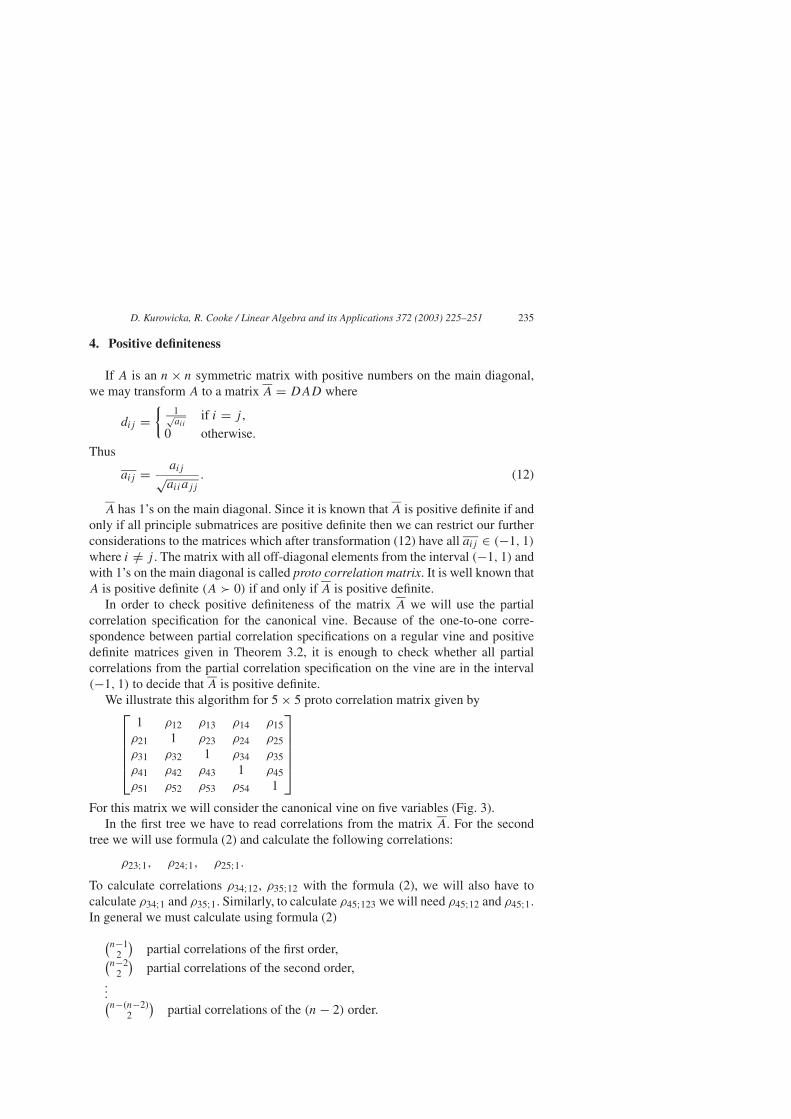
We illustrate this algorithm for 5 × 5 proto correlation matrix given by
1 ρ12 ρ13 ρ14 ρ15ρ21 1 ρ23 ρ24 ρ25ρ31 ρ32 1 ρ34 ρ35ρ41 ρ42 ρ43 1 ρ45ρ51 ρ52 ρ53 ρ54 1
For this matrix we will consider the canonical vine on five variables (Fig. 3).In the first tree we have to read correlations from the matrix A. For the second
tree we will use formula (2) and calculate the following correlations:
ρ23;1, ρ24;1, ρ25;1.To calculate correlations ρ34;12, ρ35;12 with the formula (2), we will also have tocalculate ρ34;1 and ρ35;1. Similarly, to calculate ρ45;123 we will need ρ45;12 and ρ45;1.In general we must calculate using formula (2)
(n−1
2
)partial correlations of the first order,(
n−22
)partial correlations of the second order,
...(n−(n−2)
2
)partial correlations of the (n − 2) order.

236 D. Kurowicka, R. Cooke / Linear Algebra and its Applications 372 (2003) 225–251
Fig. 3. Partial correlation specification for a canonical vine on five variables with root 1.
Hence in order to verify positive definiteness of the matrix A we have to calculate
n−2∑k=1
(n − k
2
)= (n − 2)(n − 1)n
6<
n3
6
partial correlations using formula (2).
Example 1. Let us consider the matrix
A =
25 12 −7 0.5 1812 9 −1.8 1.2 6−7 −1.8 4 0.4 −6.40.5 1.2 0.4 1 −0.418 6 −6.4 −0.4 16
and transform A to proto correlation matrix using formula (12). Then we get
A =
1 0.8 −0.7 0.1 0.90.8 1 −0.3 0.4 0.5
−0.7 −0.3 1 0.2 −0.80.1 0.4 0.2 1 −0.10.9 0.5 −0.8 −0.1 1
.
Since [ρ23;1 ρ24;1 ρ25;1ρ34;1 ρ35;1 ρ45;1
]=[0.6068 0.5360 −0.84120.3800 −0.5461 0.0281
],[
ρ34;12 ρ35;12 ρ45;12] = [0.0816 −0.0830 0.0351
],[
ρ45;123] = [0.0351
]are all between (−1, 1), it follows that, A and A are positive definite.

D. Kurowicka, R. Cooke / Linear Algebra and its Applications 372 (2003) 225–251 237
We now show the relationship between above procedure of testing positive defi-niteness and a test procedure based on the Schur complement.
Theorem 4.1 (Schur complement). Suppose that symmetric matrix M is partitionedas
M =[
X Y
Y T Z
],
where X, Z are square. Then
M � 0 ⇔ X � 0 and Z − Y TX−1Y � 0.
Let A be an n × n proto correlation matrix partitioned in the following way
A =[Xk Yk
Y Tk Zk
],
where X is k × k, 1 � k � n − 2 and Z n − k × n − k matrix.
We introduce the following notation: A;12,...,k: matrix of the kth order partial cor-relations with conditioned set {12, . . . , k}.3 If M is a square matrix with positiveelements on the main diagonal then let M denote the matrix M transformed to protocorrelation matrix using transformation (12).
Theorem 4.2.
A � 0 ⇔ ∀1�k�n−2(Zk − Y T
k X−1k Yk
) = A;12,...,k.
Proof. The proof is by iteration with respect to k. For k = 1 we get
A =[X1 Y1
Y T1 Z1
],
where
X1 = [1], Y1 = [ ρ12 ρ13 · · · ρ1n ],
Z1 =
1 ρ23 ρ24 · · · ρ2n
ρ23 1 ρ34 · · · ρ3n
· · · · · · · · · · · · · · ·ρ2,n−1 ρ3,n−1 · · · 1 ρn−1,n
ρ2n ρ3n · · · · · · 1
.
Since certainly X1 � 0, then by Theorem 4.1
A � 0 if and only if Z1 − Y T1 X−1
1 Y1 � 0.
3 Note that A;12,...,n−2 =[ 1 ρn,n−1;12,...,n−2ρn,n−1;12,...,n−2 1
].
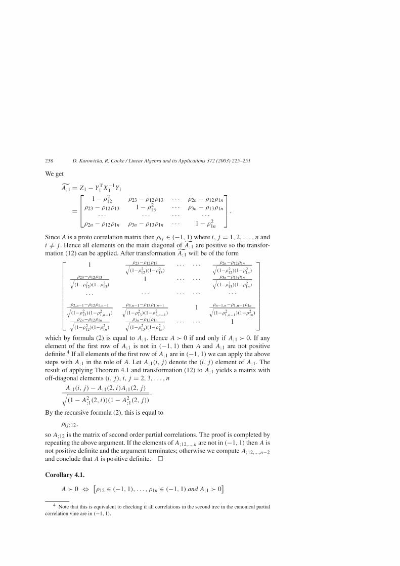
238 D. Kurowicka, R. Cooke / Linear Algebra and its Applications 372 (2003) 225–251
We get
A;1 = Z1 − Y T1 X−1
1 Y1
=
1 − ρ212 ρ23 − ρ12ρ13 · · · ρ2n − ρ12ρ1n
ρ23 − ρ12ρ13 1 − ρ213 · · · ρ3n − ρ13ρ1n
· · · · · · · · · · · ·ρ2n − ρ12ρ1n ρ3n − ρ13ρ1n · · · 1 − ρ2
1n
.
Since A is a proto correlation matrix then ρij ∈ (−1, 1) where i, j = 1, 2, . . . , n andi /= j . Hence all elements on the main diagonal of A;1 are positive so the transfor-mation (12) can be applied. After transformation A;1 will be of the form
1 ρ23−ρ12ρ13√(1−ρ2
12)(1−ρ213)
· · · · · · ρ2n−ρ12ρ1n√(1−ρ2
12)(1−ρ21n)
ρ23−ρ12ρ13√(1−ρ2
12)(1−ρ213)
1 · · · · · · ρ3n−ρ13ρ1n√(1−ρ2
13)(1−ρ21n)
. . . · · · · · · · · · · · ·ρ2,n−1−ρ12ρ1,n−1√(1−ρ2
12)(1−ρ21,n−1)
ρ3,n−1−ρ13ρ1,n−1√(1−ρ2
13)(1−ρ21,n−1)
1 ρn−1,n−ρ1,n−1ρ1n√(1−ρ2
1,n−1)(1−ρ21n)
ρ2n−ρ12ρ1n√(1−ρ2
12)(1−ρ21n)
ρ3n−ρ13ρ1n√(1−ρ2
13)(1−ρ21n)
· · · · · · 1
which by formula (2) is equal to A;1. Hence A � 0 if and only if A;1 � 0. If anyelement of the first row of A;1 is not in (−1, 1) then A and A;1 are not positivedefinite.4 If all elements of the first row of A;1 are in (−1, 1) we can apply the abovesteps with A;1 in the role of A. Let A;1(i, j) denote the (i, j) element of A;1. Theresult of applying Theorem 4.1 and transformation (12) to A;1 yields a matrix withoff-diagonal elements (i, j), i, j = 2, 3, . . . , n
A;1(i, j) − A;1(2, i)A;1(2, j)√(1 − A2
;1(2, i))(1 − A2;1(2, j))
.
By the recursive formula (2), this is equal to
ρij ;12,
so A;12 is the matrix of second order partial correlations. The proof is completed byrepeating the above argument. If the elements of A;12,...,k are not in (−1, 1) then A isnot positive definite and the argument terminates; otherwise we compute A;12,...,n−2and conclude that A is positive definite. �
Corollary 4.1.
A � 0 ⇔ [ρ12 ∈ (−1, 1), . . . , ρ1n ∈ (−1, 1) and A;1 � 0
]4 Note that this is equivalent to checking if all correlations in the second tree in the canonical partial
correlation vine are in (−1, 1).

D. Kurowicka, R. Cooke / Linear Algebra and its Applications 372 (2003) 225–251 239
⇔ [ρ23;1 ∈ (−1, 1), . . . , ρ2n;1 ∈ (−1, 1) and A;12 � 0
]...
⇔ [ρn−2,n−1;1,...,n−3 ∈ (−1, 1), ρn−2,n;1,...,n−3 ∈ (−1, 1) and
A;12,...,n−2 � 0]
⇔ ρn,n−1;12,...,n−2 ∈ (−1, 1).
5. Repairing violations of positive definiteness
In physical applications it often happens that correlations are estimated by noisyprocedures. It may thus arise that the measured matrix is not positive definite. If wewant to use this matrix we must change it to get a positive definite matrix which isas close as possible to the measured matrix.
Partial correlation specifications on a regular vine can be used to alter a non-positive definite matrix A so as to obtain a positive definite matrix B. If the matrixis not positive definite then there exists at least one element in the partial correla-tion specification of the canonical vine which is not in the interval (−1, 1). We willchange the value of that element and recalculate partial correlations on the vine usingthe following algorithm:
For 1 � s � n − 2, j = s + 2, s + 3, . . . , n
ρs+1,j ;12,...,s ∈ (−1, 1) → ρs+1,j ;12,...,s := V (ρs+1,j ;12,...,s ),
where V (ρs+1,j ;12,...,s ) ∈ (−1, 1) is the altered value of ρs+1,j ;12,...,s .Recalculate partial correlations of lower order as follows:
V (ρs+1,j ;1,...,t−1) = V (ρs+1,j ;1,...,t )
√(1 − ρ2
t,s+1;1,...,t−1
) (1 − ρ2
s+1,j ;1,...,t−1
)+ ρt,s+1;1,...,t−1ρs+1,j ;1,...,t−1, (13)
where t = s, s − 1, . . . , 1.
Theorem 5.1. The following hold:
a. all recalculated partial correlations are in the interval (−1, 1),
b. changing the value of the partial correlation on the vine leads to changing onlyone correlation in the matrix and does not effect correlations which were alreadychanged,
c. there is a linear relationship between altered value of partial correlation andcorrelation with the same conditioned set in the proto correlation matrix,
d. this method always produces a positive definite matrix.

240 D. Kurowicka, R. Cooke / Linear Algebra and its Applications 372 (2003) 225–251
Proofa. This condition follows directly from Lemma 3.6.b. The condition (b) is a result of observation that changing the value of the correl-
ation ρs+1,j ;12,...,s in the above algorithm leads to recalculate correlations of thelower order but only with the same indices before “;”, that is, s + 1, j .
c. Since ρs+1,j ;12,...,t−1 is linear in ρs+1,j ;12,...,t for all t = s, s − 1, . . . , 1 the linearrelationship between ρs+1,j and ρs+1,j ;12,...,s follows by substitution.
d. Applying the above algorithm whenever a partial correlation outside the interval(−1, 1) is found, we eventually obtain that all partial correlations in partial correl-ation specification on the vine are in (−1, 1), that is, the altered matrix is positivedefinite. �
From the statement (c) of Theorem 5.1 we can obtain the following result.
Corollary 5.1. If∣∣ρs+1,j ;12,...,s − V (ρs+1,j ;12,...,s )(1)∣∣ < ∣∣ρs+1,j ;12,...,s − V (ρs+1,j ;12,...,s )
(2)∣∣
then ∣∣ρs+1,j − ρ(1)s+1,j
∣∣ < ∣∣ρs+1,j − ρ(2)s+1,j
∣∣,where V (ρs+1,j ;12,...,s )
(1) and V (ρs+1,j ;12,...,s )(2) are two different choices of
V (ρs+1,j ;12,...,s ) in (13).
Let us consider following example:
Example 2. Let
A =
1 −0.6 −0.8 0.5 0.9−0.6 1 0.6 −0.4 −0.4−0.8 0.6 1 0.1 −0.50.5 −0.4 0.1 1 0.70.9 −0.4 −0.5 0.7 1
.
We get ρ34;12 = 1.0420 hence A is not positive definite.Since ρ34;12 > 1 then we will change its value to V (ρ34;12) = 0.9 and recalculate
lower order correlations
V (ρ34;1) = V (ρ34;12)
√(1 − ρ2
23;1)(
1 − ρ224;1)+ ρ23;1ρ24;1
and
V (ρ34) = V (ρ34;1)√(
1 − ρ213
)(1 − ρ2
14
)+ ρ13ρ14.
This way we will get for our example V (ρ34;1) = 0.9623 and finally the new valuein the proto correlation matrix V (ρ34) = 0.0293. Next we will apply the same algo-rithm to verify that this altered matrix is positive definite. We obtained matrix

D. Kurowicka, R. Cooke / Linear Algebra and its Applications 372 (2003) 225–251 241
B =
1 −0.6 −0.8 0.5 0.9−0.6 1 0.6 −0.4 −0.4−0.8 0.6 1 0.0293 −0.50.5 −0.4 0.0293 1 0.70.9 −0.4 −0.5 0.7 1
which is positive definite. Note that only cell (3, 4) is altered.
Remark 5.1. In Example 2 we could choose new value of the correlation ρ34;12,that is, V (ρ34;12) as 0.99 then the altered value of correlation ρ34 is 0.0741. If wechange ρ34;12 to 0.999 then we calculate that ρ34 is 0.0786 but in this case we ob-tain that ρ45;123 is equal −1.6224. If we change this value to −0.999 we calculateρ45 = 0.7052.
Remark 5.2. Note that the choice of vine has a significant effect on the resulting al-tered matrix. The canonical vine favors entries in the first row. They are not changed.The changes are greater the further we go from the first row. Hence when fixing amatrix one should rearrange variables to have the most reliable entries in the firstrow.
6. Completion problem
In this section we apply the canonical vine to the completion problem. First, how-ever, we quote the known results of the completion problem which can be foundin [3,5,6,9,10]. The following definitions are taken from [6]. We define the set ofcorrelation matrices En×n as follows:
En×n = {X = (xij ) symmetric n × n | X � 0, xii = 1 for all i = 1, 2, . . . , n}.
Let G = (N, E) be a graph where N = {1, 2, . . . , n}. G is simple i.e. has no loopsor parallel edges. We define the set En as a projection of En×n on the subspace RE
indexed by the edge set of G
En(G) = {x ∈ RE | ∃A = (aij ) ∈ En×n such that aij = xij for all (i, j) ∈ E}.
The sets En×n and En(G) are called eliptopes.Let G = (N, E) be a graph. Given a subset U ⊆ N , G(U) denotes the subgraph
of G induced by U , with node set U and with edge set {(u, v) ∈ E | u, v ∈ U}. Onesays that U is a clique in G when G(U) is a complete graph.
Suppose X has diagonal entries 1, and let x = (xij )ij∈E ∈ RE denote the vectorwhose components are specified entries of X. Let G denote the graph with edgeset E.
Definition 6.1. X is completable if x ∈ En(G).

242 D. Kurowicka, R. Cooke / Linear Algebra and its Applications 372 (2003) 225–251
Clique condition
x ∈ En(G) ⇒ For every clique K in G, the projection xK of x on the
edge set of K belongs to Ek(K). (14)
The clique condition is also described by saying that every fully specified principalsubmatrix is positive definite, and a matrix with this property is called partial positivedefinite. It is shown in [7] that every partial positive definite matrix whose graph isG can be completed to a positive definite matrix if and only if G is chordal (graph G
is said to be chordal if every cycle of G with length �4 has a chord; a chord of thecycle C is an edge joining two nonconsecutive nodes of C).
Since every vector x ∈ E(G) has all entries in the interval [−1, 1], we can find
ae = arccos xe
π∈ [0, 1] for every e ∈ E.
Cycle condition
x ∈ E(G) ⇒ a = (ae)e∈E satisfies condition∑e∈F
ae −∑
e∈C\Fae � |F | − 1
for C a cycle in G, F ⊆ C with |F | odd. (15)
The conditions (14) and (15) are necessary but in general not sufficient. As noted,(14) is sufficient for chordal graphs. The condition (15) is sufficient for the cyclesand series–parallel graphs i.e. graphs with no K4-minors5 [6,10]. These two con-ditions taken together suffice for describing eliptope En(G) for the graphs calledcycle completable [9] i.e. chordal graphs, series–parallel graphs and their clique sums(where clique sum of graphs G1 = (N1, E1) and G2 = (N2, E2) is a graph G =(N1 ∪ N2, E1 ∪ E2) such that the set K = N1 ∩ N2 induces a clique (possibly emp-ty) in both G1 and G2 and there is no edge between a node of N1 \ K and node ofN2 \ K).
Now we present the solution of the completion problem for the special casesof graphs using partial correlation specification of a canonical vine; the root nodeis always chosen to be 1. We shall see that verifying the relevant conditions forcompletability simultaneously gives the set of completions.
In the cases below we consider only symmetric matrices so only the upper part isshown and unspecified entries in this matrix are indicated by “�”.
5 A graph H is said to be minor of the graph G if H can be obtained from G by repeatedly deletingand/or contracting edges and deleting isolated nodes. Deleting an edge e in graph G means discarding itfrom the edge set of G. Contracting edge e = uv means identifying both end nodes of e and discardingmultiple edges and loops if some are created during the identification of u and v.

D. Kurowicka, R. Cooke / Linear Algebra and its Applications 372 (2003) 225–251 243
Case 1. We have the following partial proto correlation matrix which needs to becompleted
1 ρ12 ρ13 ρ14 · · · ρ1,k+1 ρ1,k+2 · · · ρ1n
1 ρ23 ρ24 · · · ρ2,k+1 ρ2,k+2 · · · ρ2n
· · · · · · · · · · · · · · · · · · · · ·1 ρk,k+1 ρk,k+2 · · · ρk,n
1 � · · · �· · · · · · · · ·1 � �
1 �1
.
In this case all entries in rows k + 1 to n are not specified. For n = 5 and k = 1 thiscorresponds to the graph in Fig. 4.
Since all correlations from the rows 1 to k are given we can calculate all partialcorrelations in canonical vine specifications up to (k − 1)th order.
Assigning the remaining partial correlations of order k to n − 2 in the canonicalvine any value from the interval (−1, 1), we can specify all empty cells recalculatingpartial correlations using the algorithm (13). In this case the matrix can be completedif and only if all partial correlations of order less then k are in the interval (−1, 1).Hence we must evaluate formula (2)
∑n−1j=k+1[
(j2
)− (n−k2
)] times.
Case 2a
1 ρ12 ρ13 · · · ρ1,k+1 ρ1,k+2 ρ1,k+3 ρ1,k+4 · · · ρ1n
1 ρ23 · · · ρ2,k+1 ρ2,k+2 ρ2,k+3 ρ2,k+4 · · · ρ2n
· · · · · · · · · · · · · · · · · · · · · · · ·1 ρk,k+1 ρk,k+2 ρk,k+3 ρk,k+4 · · · ρk,n
1 ρk+1,k+2 � ρk+1,k+4 · · · ρk+1,n
1 ρk+2,k+3 ρk+2,k+4 · · · ρk+2,n
1 � · · · �· · · · · · · · ·1 � �
1 �1
.
In this case all entries in rows k + 3 to n and entry (k + 1, k + 3) are unspecified. Forn = 4 and k = 1 this case corresponds to the graph on Fig. 5 (left). We can calculate
Fig. 4. Chordal graph corresponding to Case 1 with n = 5 and k = 1.

244 D. Kurowicka, R. Cooke / Linear Algebra and its Applications 372 (2003) 225–251
Fig. 5. Chordal graphs corresponding to Case 2a (left) and Case 2b (right) with n = 4 and k = 1.
all partial correlations of order less then k and all of order k except ρk+1,k+3;1,...,k .If all these partial correlations are in the interval (−1, 1) then the matrix can becompleted. To find ρk+1,k+3 we choose a value of ρk+1,k+3;1,...,k which belongs tothe non-empty interval Ik+2,k+3;1,...,k+1
6 given by (10) and then calculate ρk+1,k+3using algorithm (13). Similar solutions are obtained when the empty cell in row k + 1occupies any other position except position (k + 1, k + 2).
Case 2b
1 ρ12 ρ13 · · · ρ1,k+1 ρ1,k+2 ρ1,k+3 ρ1,k+4 · · · ρ1n
1 ρ23 · · · ρ2,k+1 ρ2,k+2 ρ2,k+3 ρ2,k+4 · · · ρ2n
· · · · · · · · · · · · · · · · · · · · · · · ·1 ρk,k+1 ρk,k+2 ρk,k+3 ρk,k+4 · · · ρk,n
1 � � ρk+1,k+4 · · · ρk+1,n
1 ρk+2,k+3 ρk+2,k+4 · · · ρk+2,n
1 � · · · �· · · · · · · · ·1 � �
1 �1
.
The difference with Case 2a is that additionally entry (k + 1, k + 2) is omitted. Forn = 4 and k = 1 this corresponds to the graph on Fig. 5 (right). In contrast to Case 2athe partial correlation ρk+1,k+2;1,...,k , which cannot be calculated now, appears in ev-ery correlation of order k + 1. To find values for correlations ρk+1,k+2 and ρk+1,k+3,we must first choose ρk+1,k+2;1,...,k such that all correlations of order k + 1 exceptρk+1,k+3;1,...,k+1 are in (−1, 1). Hence
ρk+1,k+2;1,...,k ∈ Ik+1,k+2;1,...,k = Ik+2,k+4;1,...,k+1 ∩ Ik+2,k+5;1,...,k+1 ∩ · · ·∩ Ik+2,n;1,...,k+1.
Next given this value of ρk+1,k+2;1,...,k , the value of ρk+1,k+3;1,...,k can be found. Inthis case the matrix can be completed if all correlations which can be computed arein (−1, 1) and if the interval Ik+1,k+2;1,...,k is not empty.
6 We write Ik+1,k+2;1,...,k instead of Iρk+1,k+2;1,...,k.

D. Kurowicka, R. Cooke / Linear Algebra and its Applications 372 (2003) 225–251 245
Case 3. This case is an example of non-chordal graph with one cycle with length 4:
1 ρ12 ρ13 · · · ρ1,k+1 ρ1,k+2 ρ1,k+3 ρ1,k+4 · · · ρ1n
1 ρ23 · · · ρ2,k+1 ρ2,k+2 ρ2,k+3 ρ2,k+4 · · · ρ2n
· · · · · · · · · · · · · · · · · · · · · · · ·1 ρk,k+1 ρk,k+2 ρk,k+3 ρk,k+4 · · · ρk,n
1 ρk+1,k+2 � ρk+1,k+4 · · · ρk+1,n
1 ρk+2,k+3 � · · · ρk+2,n
1 ρk+3,k+4 · · · ρk+3,n
· · · · · · · · ·1 � �
1 �1
.
We can see that rows k + 3 to n and entries (k + 1, k + 3) and (k + 2, k + 4) areunspecified. For k = 1 and n = 5 this corresponds to the graph on Fig. 6 (left). Inthis case we can calculate all partial correlations of order less than k and all of orderk except ρk+1,k+3;12,...,k and ρk+2,k+4;12,...,k .
Using Lemma 3.7 we choose ρk+1,k+3;12,...,k belonging to the intersection
Ik+1,k+3;12,...,k = Ik+2,k+3;12,...,k+1 ∩ Ik+3,k+4;1,...,k+1
of two intervals such that ρk+2,k+3;12,...,k+1 and ρk+3,k+4;12,...,k+1 are in (−1, 1) ifthis intersection is non-empty. We next can find possible solutions forρk+3,k+4;12,...,k+1such that ρk+3,k+4;12,...,k+2 is in (−1, 1). Recalculating correlations using formula(13) we can fill empty cells in the cycle. In this case the matrix can be completedif all correlations which can be calculated are in (−1, 1) and if Ik+1,k+3;1,...,k is notempty. If the intersection of Ik+2,k+3;1,...,k+1 and Ik+3,k+4;1,...,k+1 is empty then thismatrix cannot be completed (see Example 4).
Remark 6.1. We notice that the procedure of finding correlation ρk+1,k+3;12,...,k
which belongs to the interval Ik+1,k+3;12,...,k allows us to choose a chord in thiscircuit. In this way, Case 3 can be reduced to the previous cases where chordal graphswere considered.
In Section 3 of [10] the completion problem for a cycle was solved. The approachused in [10] consist of solving a system of equations which is equivalent to (16).
Fig. 6. Graphs corresponding to Case 3 (left) with k = 1, n = 5 and Case 4 (right) with n = 6.

246 D. Kurowicka, R. Cooke / Linear Algebra and its Applications 372 (2003) 225–251
In Case 4 we present this approach in terms of partial correlation specification on avine.
Case 4. In this case we show the general solution of the completion problem for thecycle of length n (n � 4). The following matrix corresponds to the cycle of length n
(the cycle of length 6 is presented on Fig. 6 (right)),
1 ρ12 � � · · · � ρ1n
1 ρ23 � · · · � �· · · · · · · · · · · · · · ·
1 ρn−3,n−2 � �1 ρn−2,n−1 �
1 ρn−1,n
1
.
We have to choose correlations ρ13, ρ14, . . . , ρ1,n−1 such that by Lemmas 3.7 and3.8 the following system is satisfied
ρ13 ∈ I23;1,(ρ13, ρ14) ∈ A(ρ34),
(ρ14, ρ15) ∈ A(ρ45),
· · ·(ρ1,n−2, ρ1,n−1) ∈ A(ρn−2,n−1),
ρ1,n−1 ∈ In−1,n;1,
(16)
where I23;1 denotes Iρ23;1 .If we can solve (16) then this matrix can be completed. We complete our matrix
with the algorithm presented below:
ρ34;12 ∈ (−1, 1) ⇔ ρ24;1 ∈ I34;12 ⇒ ρ24 can be calculated with (13),
ρ35;12 ∈ (−1, 1) ⇔ ρ25;1 ∈ I35;12 ⇒ ρ25 can be calculated,
· · ·ρn−1,n;12 ∈ (−1, 1) ⇔ ρ2n;1 ∈ In−1,n;12 ⇒ ρ2n can be calculated,
ρ45;123 ∈ (−1, 1) ⇔ ρ35;12 ∈ I45;123 ⇒ ρ35;1 and next ρ35 can be calculated,
· · ·ρn−1,n;123 ∈ (−1, 1) ⇔ ρ3n;12 ∈ In−1,n;123 ⇒ ρ3n;1 and next ρ3n can be calculated,
· · ·ρn−1,n;12,...,n−2 ∈ (−1, 1) ⇔ ρn−2,n;12,...,n−3 ∈ In−1,n;12,...,n−2 ⇒ ρn−2,n;12,...,n−4
and next ρn−2,n;12,...,n−4, . . . , ρn−2,n can be calculated.
Case 5. In this case we consider wheel on n (n � 4) elements (a wheel on n ele-ments is a graph composed of a circuit C on n − 1 nodes together with an additionalnode adjacent to all nodes of C).

D. Kurowicka, R. Cooke / Linear Algebra and its Applications 372 (2003) 225–251 247
The following matrix corresponds to the wheel of length n
1 ρ12 ρ13 ρ14 ρ15 · · · · · · ρ1,n1 ρ1n
1 ρ23 � � · · · · · · � ρ2n
1 ρ34 � · · · · · · � �· · · · · · · · · · · · · · · · · ·
1 ρn−3,n−2 � �1 ρn−2,n−1 �
1 ρn−1,n
1
.
This case can be reduced to the Case 5 by applying Theorem 4.1. If correlationsρk,k+1;1 for k = 2, 3, . . . , n − 1 and ρ2n;1 are in (−1, 1) then the following matrixneeds to be completed
1 ρ23;1 � � · · · � ρ2n;11 ρ34;1 � · · · � �
· · · · · · · · · · · · · · ·1 ρn−2,n−1;1 �
1 ρn−1,n;11
.
Remark 6.2. Note that it is shown in [10] that the wheel on n (n � 5) elements isnot cycle completable.
Remark 6.3. To our knowledge Case 5 is the first method for completing the wheel.Methods of completing chordal graphs and cycles have been previously presented in[7,10].
Example 3. The following matrix corresponds to a wheel on six elements (Fig. 7)
Fig. 7. A wheel on six elements.

248 D. Kurowicka, R. Cooke / Linear Algebra and its Applications 372 (2003) 225–251
1 ρ12 ρ13 ρ14 ρ15 ρ161 ρ23 � � ρ26
1 ρ34 � �1 ρ45 �
1 ρ561
=
1 0.8 0.1 −0.3 0.5 −0.41 0 � � −0.1
1 −0.6 � �1 −0.7 �
1 0.21
.
We can calculate[ρ23;1 ρ26;1 ρ34;1 ρ45;1 ρ56;1
]= [−0.1340 0.4001 −0.6005 −0.6658 0.5040
].
We must choose correlations ρ24;1 and ρ25;1 such that the system similar to (16) issatisfied. Since ρ24;1 ∈ I34;12 = (−0.7119, 0.8729) and ρ25;1 ∈ I56;12 = (−0.5899,
0.9932) then we can choose ρ24;1 = ρ25;1 = 0. Hence ρ34;12 = −0.6060, ρ45;12 =−0.6658 and ρ56;12 = 0.5499. (Note that ρ45;12 depends on ρ24;1 and ρ25;1. Hencewe must choose these correlations such that also ρ45;12 ∈ (−1, 1). If it is not possiblethen this graph cannot be completed.)
Now we can find ρ35;12 ∈ I45;123 = (−0.1900, 0.9970). Let us choose ρ35;12 = 0then ρ45;123 = −0.8370 and ρ36;12 ∈ I56;123 = (−0.8352, 0.8352). Hence we canalso take ρ36;12 = 0 then ρ56;123 = 0.5499. Finally we get ρ46;123 ∈ I56;1234 =(−0.9173, −0.0032). We take for instance ρ46;123 = −0.5 and now we can recal-culate all correlations using algorithm (13).
ρ24;1 = 0⇒ρ24 = ρ12ρ14 = −0.24,
ρ25;1 = 0⇒ρ25 = ρ12ρ15 = 0.4,
ρ35;12 = 0⇒ρ35;1 = ρ23;1ρ25;1 = 0
⇒ρ35 = ρ13ρ15 = 0.05,
ρ36;12 = 0⇒ρ36;1 = ρ23;1ρ26;1 = −0.0536
⇒ρ36 = ρ36;1√(
1 − ρ213
)(1 − ρ2
16
)+ ρ13ρ16 = −0.0889,
ρ46;123 = −0.5⇒ρ46;12 = −0.3977 ⇒ ρ46;1 = −0.3645
⇒ρ46 = −0.1987.
We obtain that the matrix
1 0.8 0.1 −0.3 0.5 −0.41 0 −0.24 0.4 −0.1
1 −0.6 0.05 −0.08891 −0.7 −0.1987
1 0.21
is positive definite.

D. Kurowicka, R. Cooke / Linear Algebra and its Applications 372 (2003) 225–251 249
Example 4. Let us consider the following matrix
1 ρ12 ρ13 ρ14 ρ151 ρ23 � ρ25
1 ρ34 �1 ρ45
1
=
1 0.7 −0.3 0.2 0.51 −0.8 � 0.7
1 0.6 �1 0.9
1
which corresponds to the Case 3 with n = 5 and k = 1. We can calculate[ρ23;1 ρ25;1 ρ34;1 ρ45;1
] = [−0.8661 0.5659 0.7061 0.9428].
Now following the procedure presented in Case 3 we must choose correlation ρ24;1such that it belong to the intersection of I34;12 and I45;12. We get however that
I34;12 = (−0.9655, −0.2576),
I45;12 = (0.2587, 0.8084).
Hence the intersection is empty. From this we conclude that this matrix cannot becompleted.
General solution strategyWe consider a practicable strategy for finding a completion of an incomplete proto
correlation matrix, if such a solution exists. The following matrix is given (assumedto be symmetric)
1 ρ12 ρ13 · · · ρ1,n−1 ρ1n
ρ21 1 ρ23 · · · ρ2,n−1 ρ2n
ρ31 ρ32 1 · · · ρ3,n−1 ρ3n
. . . · · · · · · · · · · · · · · ·ρn−1,1 ρn−1,2 ρn−1,3 · · · 1 ρn−1,n
ρn1 ρn2 ρn3 · · · ρn,n−1 1
.
First, we remark that by Lemma 3.7 we know that if the matrix is completable,then the set of solutions is open. Some of the entries ρij are not specified. We firstorder the rows and columns to obtain a maximal bottom right triangle above the dia-gonal with unspecified elements. If all unspecified cells appear in this triangle, thenthe choices of values for the partial correlations whose conditioned sets correspondwith the empty cells is unconstrained (Case 1). Any choice yields a completion under(2). If there is an unspecified cell (i, j) such that some (i, k) is specified, k > j , thenthe choice of partial correlations ρij ;1,...,i−1 is constrained. The different ways inwhich these are constrained are illustrated in the cases above. In general, we can saythat for all unspecified cells in the ith row, ρij ;1,...,i−1 must be chosen such that allpartial correlations ρkj ;1,...,i , k > i are in (−1, 1).
Define Ck = {j ∈ {k + 1, . . . , n} | ρkj unspecified} and Dj = {k ∈ {j + 1, . . . ,
n} | ρkj specified}. To choose values for ρ1j , j ∈ C1 we must solve a system suchthat all correlations of the first order ρkj ;1 are in the interval (−1, 1), where k ∈ Dj ,

250 D. Kurowicka, R. Cooke / Linear Algebra and its Applications 372 (2003) 225–251
using Lemma 3.7 and/or Lemma 3.8. (If the system has no solutions, the matrix isnot completable.) If this system has solutions then we can fill all empty cells in thefirst row and the values of ρkj ;1 are fixed. Next we repeat the same operation forthe unspecified elements in the second row ρ2j , j ∈ C2. We must solve a systemsuch that all correlations of the second order ρkj ;12 where k ∈ Dj are in the interval(−1, 1). If this system has solutions we obtain partial correlations of the first orderρ2j ;1. If this system has no solutions, we return to C1 and choose another solution,re-fixing the values of ρkj ;1. If the matrix is completable, we can find a solution forC1 which allows us to fix values for C2 in finitely many steps. We continue in thisway through row n. Of course this strategy is not an effective procedure for decidingwhether or not a given incomplete matrix is completable. The issue of decidabilityof real closed fields is not addressed in this paper.
7. Conclusions
We have explained the use of partial correlation specifications on a canonicalvine in various problems regarding positive definiteness of proto correlation matri-ces. One attractive feature is that the steps in the algorithms acquire a probabilisticinterpretation through the notion of partial correlations. We note, however, that theycannot apply to problems involving positive semidefiniteness. Indeed, the denom-inators in (2) must be non-zero and this implies that all partial correlations mustbe greater than −1 and less than 1. The speed of these algorithms appears to becomparable to that of previous algorithms.
Acknowledgements
The authors would like to thank Monique Laurent, Etienne de Klerk, Erling An-dersen for helpful discussions. We would like to acknowledge the conscientious ef-fort the referee has put into this paper.
References
[1] R.M. Cooke, Markov and entropy properties of tree and vines-dependent variables, in: Proceedingsof the ASA Section of Bayesian Statistical Science, 1997.
[2] D. Kurowicka, R. Cooke, Conditional and partial correlation for graphical uncertainty models,in: Proceedings of the 2nd International Conference on Mathematical Methods in Reliability,Birkhäuser, 2000.
[3] M. Fiedler, Matrix inequalities, Numer. Math. 9 (1966) 109–119.[4] G.U. Yule, M.G. Kendall, An introduction to the theory of statistics, 14th ed., Charles Griffin & Co.,
Belmont, CA, 1965.[5] M. Laurent, Cuts, matrix completions and graph rigidity, Math. Program. 79 (1997) 255–283.[6] M. Laurent, The real positive semidefinite completion problem for series–parallel graphs, Linear
Algebra Appl. 253 (1997) 347–366.

D. Kurowicka, R. Cooke / Linear Algebra and its Applications 372 (2003) 225–251 251
[7] R. Grone, C.R. Johnson, E.M. Sá, H. Wolkowicz, Positive definite completions of partial hermitianmatrices, Linear Algebra Appl. 58 (1984) 109–124.
[8] T.J. Bedford, R.M. Cooke, Vines—a new graphical model for dependent random variables, Ann.Statist. 30 (4) (2002) 1031–1068.
[9] W. Barrett, C.R. Johnson, R. Loewy, The real positive definite completion problem: cycle completa-bility, Mem. Amer. Math. Soc. 584 (1996) 69.
[10] W. Barrett, C.R. Johnson, P. Tarazaga, The real positive semidefinite completion problem for se-ries–parallel graphs, Linear Algebra Appl. 192 (1993) 3–31.