Muther.L;iicul Modelling. Vol. 3, pp. 69-81. 1982 0270_0255/82/01ou69-13$03.00/0 P+ted in the USA. All rIghI\ reserved Copyright @ 19112 Pergamon Press Ltd.

’ RECIPROCAL MATRICES WITH RANDOM COEFFICIENTS

LUIS G. VARGAS

University of Pittsburgh Pittsburgh, Pennsylvania 15260, USA

Communicated by Thomas L. Saaty

Abstract-A method is developed to estimate the average opinion (or core) of a group of people. The method elicits judgments from a smaller group of individuals than the total population. What we obtain is a scattering of values around a core value that is being estimated. Some of those values will be closer to the core and others will lie away from it. The method presented here allows us, given the density of concentration of the judgments, to use to a greater extent those values closer to the core. The method generates a surface which is more like a probability distribution that can be used to estimate the core without treating the data as if it were direct estimates of it. The shape of the distribution that we have shown to be the relevant one is that corresponding to a Dirichlet distribution. Here we show that the only distribution of judgments which yields this type of result is the gamma distribution. Under the assumption of total consistency, if the judgments are gamma distributed, the principal right-eigenvector of the resulting reciprocal matrix of pairwise comparisons is Dirichlet distributed. If the assumption of consistency is relaxed, then the hypothesis that the principal right-eigenvector follows a Dirichlet distribution is accepted if inconsistency is 10% or less.

1. INTRODUCTION

A random reciprocal matrix X is a matrix whose coefficients’are random variables and satisfy the property Xij = I/X,, for all i, j = I,2 ~ . ~ n. Such a matrix is used in the Analytic Hierarchy Process to prioritize alternatives using pairwise comp,arison judg- ments elicited from decision makers or other experienced judges. These judgments are arranged in the form of a reciprocal matrix whereby both the judgment and its reciprocal value are entered simultaneously. The principal right eigenvector of such a matrix is the vector of priorities (weights or relative importance) which scales decision makers’ preference among the activities. Thus, if X is the matrix of preferences, and % the vector of priorities, we have X8 = A,,,,,%, where Amax is the largest eigenvalue of X. If the matrix X satisfies XijXjk = Xik, for all i, j, k = 1,2 o . D n, then X is said to be consistent. In this case A,,, = n and the entries of X can be written as the ratios of the components of its principal right eigenvector, Ecij, i.e., Xii = Wi/Wj, i, j = I,2 . . D n. A more detailed analysis of reciprocal matrices, and their importance in the Analytic Hierarchy Process is given in Saaty [I].

Our object is to study reciprocal matrices whose entries are random variables. This would allow us to simulate the behavior of decision makers by establishing probability distributions of the resulting vector of priorities. These distributions would be useful in estimating the PR-eigenvector in behavioral situations which involve a large number of decision makers with diverse opinions.

2. DISTRIBUTION OF THE PRINCIPAL RIGHT EIGENVECTOR: THE PARADIGM CASE

Let us start by analyzing the simplest case-when the matrix of preferences X is consistent. In this case the entries of X satisfy

X,Xi, = Xik, i, j, k = 1.2 . . . n.

69

70 Lurs G. VARGAS

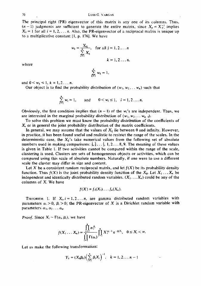
The principal right (PR) eigenvector of this matrix is (n - 1) judgments are sufficient to generate the entire Xii = 1 for all i = 1,2,. . . n. Also, the PR-eigenvector of to a multiplicative constant [l, p. 1761. We have

wr,=_x’“, forall j=1,2.

z xir

any one of its columns. Thus, matrix, since Xii = Xi! implies a reciprocal matrix is unique’up

. . n

where

Our object is to find the probability distribution of (wr, w2. . . w,) such that

&wi=l, and O<WiSl, i=1,2...n.

Obviously, the first condition implies that (n - 1) of the wi’s are independent. Thus, we are interested in the marginal probability distribution of (w,, ~2. . . wn-,).

To solve this problem we must know the probability distribution of the coefficients of X, or in general the joint probability distribution of the matrix coefficients.

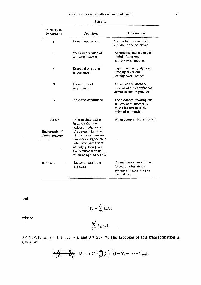
In general, we may assume that the values of Xii lie between 0 and infinity. However, in practice, it has been found useful and realistic to restrict the range of the’scales. In the deterministic case, the Xii’s take numerical values from the following set of absolute numbers used in making comparisons: b,f . . . f, 1,2 . . .8,9. The meaning of these values is given in Table 1. If two activities cannot be compared within the range of the scale, clustering is used. Clusters are sets of homogeneous objects or activities, which can be compared using this scale of absolute numbers. Naturally, if one were to use a different scale the cluster may differ in size and content.

Let X be a consistent random reciprocal matrix, and let f(X) be its probability density function. Thus f(X) is the joint probability density function of the Xii. Let Xr . . . X, be independent and identically distributed random variables. (Xi . . . X,) could be any of the columns of X. We have

f(X) = fl(Xl) . . . f”W”).

THEOREM 1. If Xi, i = 1,2. . . n, are gamma distributed random variables with parameters tii > 0, pi > 0; the PR-eigenvector of X is a Dirichlet random variable with parameters czlr cz2.. . a,.

Proof. Since Xi - T(Cri, pi), we have

flapi ”

f(X, . . . X”) = r=l l i rc ,,J Xg'-'empixf, OlXi <w. al

i=l

Let us make the following transformation:

Reciprocal matrices with random coefficients

Table 1.

71

Intensity of Importance Definition Explanation

1 Equal importance

3 Weak importance of one over another

Essential or strong. importance

Demonstrated importance

Absolute importance

W,O

Reciprocals of above nonzero

Intermediate values between the two adjacent judgments If activity i has one of the above nonzero numbers assigned to it when compared with activity j, then j has the reciprocal value when compared with i.

Rationals Ratios arising from the scale

Two activities contribute equally to the objective

Experience and judgment slightly favor one activity over another.

Experience and judgment strongly favor one activity over another

An activity is strongly favored and its dominance demonstrated in practice

The evidence favoring one activity over another is of the highest possible order of affirmation.

When compromise is needed

If consistency were to be forced by obtaining n numerical values to span the matrix.

and

where ii-l

,F, yk<l,

o<&;,<l,for k=l,2...n- 1, and 0 I Y. < 03. The Jacobian of this transformation is given by

3(X,...X,) c?(Y, * *. Y")

= (.JI = Y i-’ (fi pi)-‘(1 - YI - ’ * ‘-Yn-,)*

12

Thus, we have

LUIS G. VARGAS

Hence, the marginal distribution of (Y,, Yt . . . Y,,-i) is

G,-,(Y,. . . Y,_,) = r(aln+ * * ‘+an)n-’ Q Uai)

where Yk>09 k=1,2...n-l,and

which corresponds to parameters LYI . . . an.

F yk<l,

the probability density function of a Dirichlet distribution with

THEOREM 2. Let (Y,. . . Y,-1) be an (n - 1)-dimensional variable with a Dirichlet distribution of parameters ol . . . an. The variables Yk, k = 1,2. . . n - 1 are distributed according to a beta distribution,

Proof. We define the variables

Z,=Y,,(l-Y‘.)-‘, k=1,2...n-1 h# k.

Then, the Jacobian of the transformation is

IJ\ = (1 - Yk)“-‘,

and, we have

f k

3. GENERALIZATION: THE INCONSISTENT CASE

Let us now consider an arbitrary random reciprocal matrix, X, i.e., there exist some i, j, and k for which xijxjk# Xik.

To obtain the distribution of the principal right eigenvector of X, \ii, we must consider n(n - 1)/2 independent random variables. In this case the PR-eigenvector must be obtained by solving the stochastic system of equations

s Xijwj = &naxWi,

Reciprocal matrices with random coefficients 73

i=l,2... n, where A,, is the principal eigenvalue of X. A,, is also a random variable whose distribution depends on the distribution of the Xij’s. There is not an easy answer for this case. However, we can use an approximation of the PR-eigenvector to obtain an estimate of its distribution.

The average of normalized columns of a reciprocal matrix provides a good estimate of the PR-eigenvector in the deterministic case [see 1, p. 2341, i.e.,

gJi = , i=1,2...n.

If the Xii are gamma random variables we found that

Xj

follow a Dirichlet distribution. Thus, the distribution of \isi is the convolution of n

Dirichlet random variabks, which in general is not a Dirichlet distribution. A way of circumventing this problem is by examining the consistency of the matrix of

expected values and deciding when such a matrix is sufficiently consistent to justify the assumption that the PR-eigenvector would also be a Dirichlet random variable.

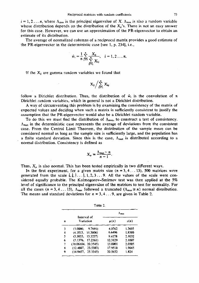
To do this we must find the distribution of A,,,,, to construct a test of consistency. A,,, in the deterministic case represents the average of deviations from the consistent case. From the Central Limit Theorem, the distribution of the sample mean can be considered normal as long as the sample size is sufficiently large, and the population has a finite standard deviation. Since this is the case; A,,,= is distributid according to a normal distribution. Consistency is defined as

Thus, X,, is also normal. This has been tested empirically in two different ways. In the first experiment, for a given matrix size (n = 3,4 _ a a 13), 500 matrices were

generated from the scale i 6 4 : I,2,3 *OD 9 . . _ 9, All the values of the scale were con- sidered equally probable. Ghk Kolmogorov-Smirnov test was then applied at the 5% level of significance to the principal eigenvalue of the matrices to test for normality. For all the cases (n = 3,4. . . Ia), A,,, followed a truncated (h,.,,ax 2 n) normal distribution. The means and standard deviations for n = 3,4 e . .9, are given in Table 2.

Table 2.

A max

Interval of

n Variation CL(n) s(n)

3 (3.0000, 9.7691) 4.0762 1.3695 4 (4.1013, 11.3006) 6.6496 1 A380

5 (5.3855, 15.3237) 9.4178 2.1032

6 (7.1376, 17.2361) 12.3129 2.1007

7 (10.06104, 20.3545) 15.0001 2.0305

8 (12.4807, 23.5383) 17.9518 1.9045 9 (14.9457, 25.3345) 20.5652 1.824

74 LUIS G. !‘ARGAS

The second experiment used a specific (gamma) distribution to obtain the entries of the randomly generated matrices. The sample size in this case was n = 100. Once more

.Imirx fit a truncated normal distribution at the 5% level of significance. Since in the second case we specify the distribution and its parameters, we decided to use the results of the first experiment, which are distribution free, to construct a consistency test.

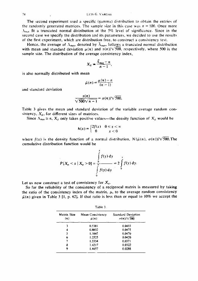
Hence, the average of Amax, denoted by x,,,, follows a truncated normal distribution with mean and standard deviation p(n) and s(n)/%%% respectively, where 500 is the sample size. The distribution of the average consistency index,

is also normally distributed with mean

and standard deviation

CL(n)- n P(n) = (n _ ,)

s(n) - = cr(n)/V/soo.

diiiWn - 1

Table 3 gives the mean and standard deviation of the variable average random con- sistency, XC, for different sizes of matrices.

Since Amax 2 n, XG only takes positive values-the density function of XG would be

h(x)= o 1 2fCx) 05x <r: x<o

where f(x) is the density function of a normal distribution, N(@(n). a(n))/q/500.The cumulative distribution function would be

x

I f(y)dy .x

P[X,<x IX,>O]= : = 2

I

I f(y)0

f(y)dy ’

0

Let us now construct a test of consistency for X6. So far the reliability of the consistency of a reciprocal matrix is measured by taking

the ratio of the consistency index of the matrix, CL, to the average random consistency fi(n) given in Table 3 [l, p_ 621. If that ratio is less than or equal to 10% we accept the

Table 3

Matrix Size Mean Consistency Standard Deviation

(n) C(n) ~(nwm

3 0.5381 0.0433 4 0.8832 0.0475 5 I.1045 0.0470 6 I .2525 0.0420 7 1.3334 0.037 I 8 1.4217 0.0322 9 I .4457 0.0288

Reciprocal matrices with random coefficients 15

Table 4.

Matrix Size Acceptance

(n) Region (a = 5%)

3 0.04532 4 0.07901 5 0.10124 6 0.11803 I 0.12511 8 O.L3586 9 0.13904

Bound of

Am,X

3.09064 4.23703 5.404% 6.59015 I.75066 8.95102

10.11232

results as being sufficiently consistent Let us construct a (I- at)% confidence interval of the ratio p/X,, where p is not a random variable. We have

P[$+j =P[Xi+ Xp is a truncated normal distribution N@(n), a’(n)), where a’(n) = o(n)/v/soo. Stan- dardizing X, we have

At a level of significance of cy%, we have

and

or

CL = r@(n) - Izab’(n)l.

The upper bounds of consistency for y = 0.10 are given in Table 4. Thus, for a given reciprocal matrix, we accept the hypothesis Ho: p/X$5 y if the

consistency of the matrix, p, is smaller than the upper bounds given in Table 4.

4. A BOUND OF RANDOM CONSISTENCY

Let us now examine why y should be 10%. To do this we have selected (3 x 3)

matrices. An obvious reason to select this matrix size is because any 3 X 3 reciprocal matrix X can be decomposed as follows:

76 LUIS G. VARGAS

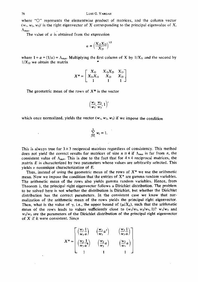
where “0” represents the elementwise product of matrices, and the column vector (w,, w2, w$ is the right eigenvector of X corresponding to the principal eigenvalue of X, A max.

The value of a is’obtained from the expression

a = (y23)“’

where 1 + a + (l/a) = Amax. Multiplying the first column of X by 1/X3, and the second by l/X32 we obtain the matrix .

x13 x12x23 xi3 x*= x21x13 x23 x23

1 1 1 1 The geometric mean of the rows of X* is the vector

which once normalized, yields the vector (WI, ~2, ~3) if we impose the condition

This is always true for 3 x 3 reciprocal matrices regardless of consistency. This method does not yield the correct results for matrices of size n Z- 4 if Amax is far from n, the consistent value of Amax. This is due to the fact that for 4 x 4 reciprocal matrices, the matrix E is characterized by two parameters whose values are arbitrarily selected. This yields a nonunique characterization of E.

Thus, instead of using the geometric mean of the rows of X* we use the arithmetic mean. Now we impose the condition that the entries of X* are gamma random variables. The arithmetic mean of the rows also yields gamma random variables. Hence, from Theorem 1, the principal right eigenvector follows a Dirichlet distribution. The problem to be solved here is not whether the distribution is Dirichlet, but whether the Dirichlet distribution has the correct parameters. In the consistent case we know that nor- malization of the arithmetic mean of the rows yields the principal right eigenvector. Then, what is the value of y, i.e., the upper bound of (p/X@), such that the arithmetic mean of the rows leads to values sufficiently close to (WI/WJ, w2/w3, l)? wt/w~ and w2/w3 are the parameters of the Dirichlet distribution of the principal right eigenvector of X if it were consistent. Since

Reciprocal matrices with random coefficients 77

the arithmetic mean of the rows are

and the estimated principal right eigenvector W follows a Dirichlet distribution D(&i, &, hi,). The solution to the stochastic problem Xw = Amax w, follows a Dirichlet distribution

4 a,=$,a*=q_x3=1f w3 )

We want &i, i = I, 2,3, to be as close to DL~, i = I,%, 3, as possible SO that both distributions coincide, i.e., can we accept the hypothesis Ho: D = B?

Let 6 be an upper bound of the percent deviation of &i9 I’ = 1,2,3, from oi, i = I, 2,3; i.e.,

If 8 = 0.10, then a = 1-k f. Note that for 8 = 0 we have a = 1, and the matrix X is consistent. For a = 1-k 4,

A - 3.0833, and p. = 0.0417. Thus we have max -

0.0417 $ = 0.5381- 1.96C.0433) = o’0919

at a level of significance a = 0.05. Thus, for n = 3, fit&) and D(ai) can be assumed to be the same as long as

p/X& < 0.20. For n 2 4, the characterization of the upper bound of p/Xp is rather complex and the results do not point towards a conclusion as clear as for n = 3.

Some statistical tests for matrices of size n 2 4, point towards an increase of the bound on p/XIz up 20%, for matrices hypothesis

to 20%. All tests performed by fixing the level of consistency above generated according to gamma distributions, failed to accept the

Hence, selecting p/X& < 0.10, we are then sure that the hypothesis is accepted for all values of ~1. For example, let us consider the 3 x 3 reciprocal matrix

78 LUISG.VARGAS

where the principal eigenvector is w = (0.65, 0.29, 0.06) and A,,, = 3.0735. Thus, we have I_L = 0.0368, and p/Xp = 0.0368/0.4532 = 0.0811< 0.10. X can be decomposed as follows,

1 1.31 0.76

0.76 1 1.31 1.31 0.76 1 1 x= X 0 E

Thus, we have

8 18 8

X* = [ 813 6 6 1 1 1 1 and

ai, = 11.33

aiz = 4.89

&3= 1

The estimated Dirichlet distribution is

[&,I = 11

[&I = 5

[&I = 1

rj(ll, 5, 1).

The real Dirichlet distribution of w is D([aJ, [az], I), where

[all = [ 10.83]= 11

[azj.= E4.833 = 5

[aj] = [Xl = 1

Let us now consider the matrix

A B C

I

with principal eigenvector w = (0.6223, 0.2470, 0.1307)’ and A,,, = 3.2174. Thus, we have p = 0.1087 and w/Xi, = 0.108710.4532 = 0.2398 > 0.10. w follows the Dirichlet distribution D(5, 2, 1) if X were consistent. However, we have

3 12 3

x* = [ 314 3 3

1 1 1 I which yields

di, =6 [&,I = 6

aia = 2714 [a;*] = 2

&,= 1 [&I = 1

Reciprocal matrices with random coefficients 19

and the Dirichlet distribution of the estimate eigenvector G is &6,2,1) which is not the same as D(5.2, I).

In general, let us denote by X, a consistent reciprocal matrix whose entries are the expected values of gamma distributed variables. If we generate random matrices using X, as the parameters of gamma distributions, then the average PR-eigenvector of the sample tends to the PR-eigenvector of Xc as inconsistency decreases.

If X, is an arbitrary reciprocal matrix, then the distribution of its PR-eigenvector depends on its consistency; and the distribution of the average PR-eigenvector does not necessarily converge to that of X,.

This analysis can be extended to a hierarchic structure to study its stability. The stability of a hierarchy can be analyzed from different points of view:

(a) Stability with respect to change in the composition of its levels (structural stability);

(b) Stability with respect to changes in judgements (sensitivity analysis) 121; and (c) Stability in time. Our analysis can be used to study the stability of a hierarchy from the second point of

view. That is, if we consider the priorities fixed, what is the possible range of judgments ’ which produce the same result, and given specific changes in the final composite vector, which judgments ought to be changed to attain the desired fluctuation maintaining consistency below a certain level.

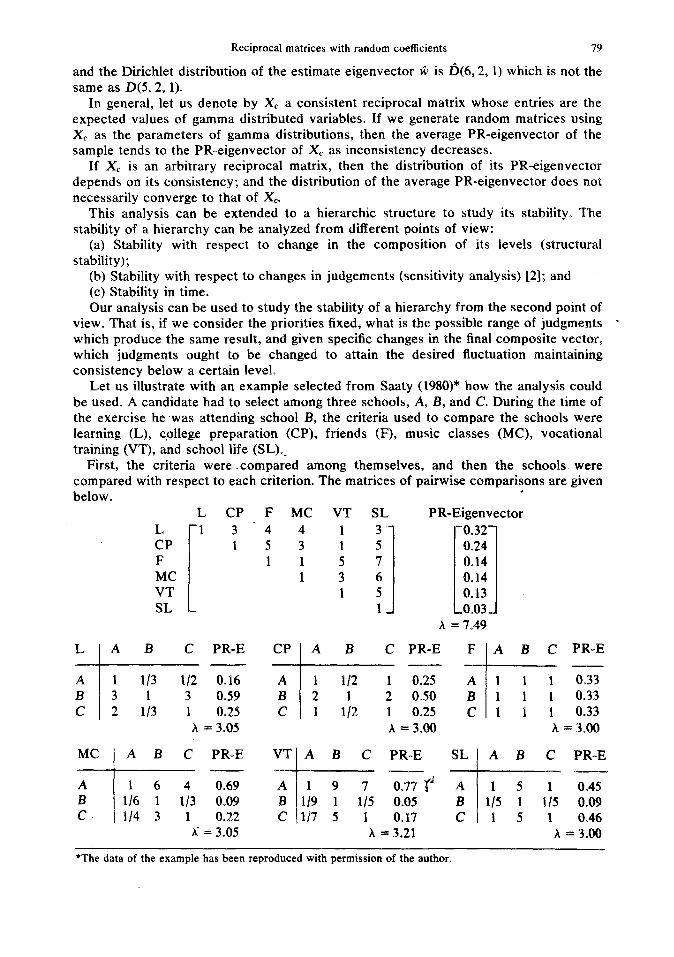
Let us illustrate with an example selected from Saaty (1980)* how the analysis could be used. A candidate had to select among three schools, A, B, and C. During the time of the exercise he .was attending school B, the criteria used to compare the schools were learning (L), cpllege preparation (CP), friends (F), music classes (MC), vocational training (VT), and school life (SL)-_

l?irst, the criteria were .compared among themselves, ?nd then the schools were compared with respect to each criterion. The matrices of pairwise comparisons are given below.

.

L CP F MC VT SL PR-Eigenvector

5[‘G’K] ~~

A = 3149

*The data of the example has been reproduced with permission of the author.

80 LUIS G. VARGAS

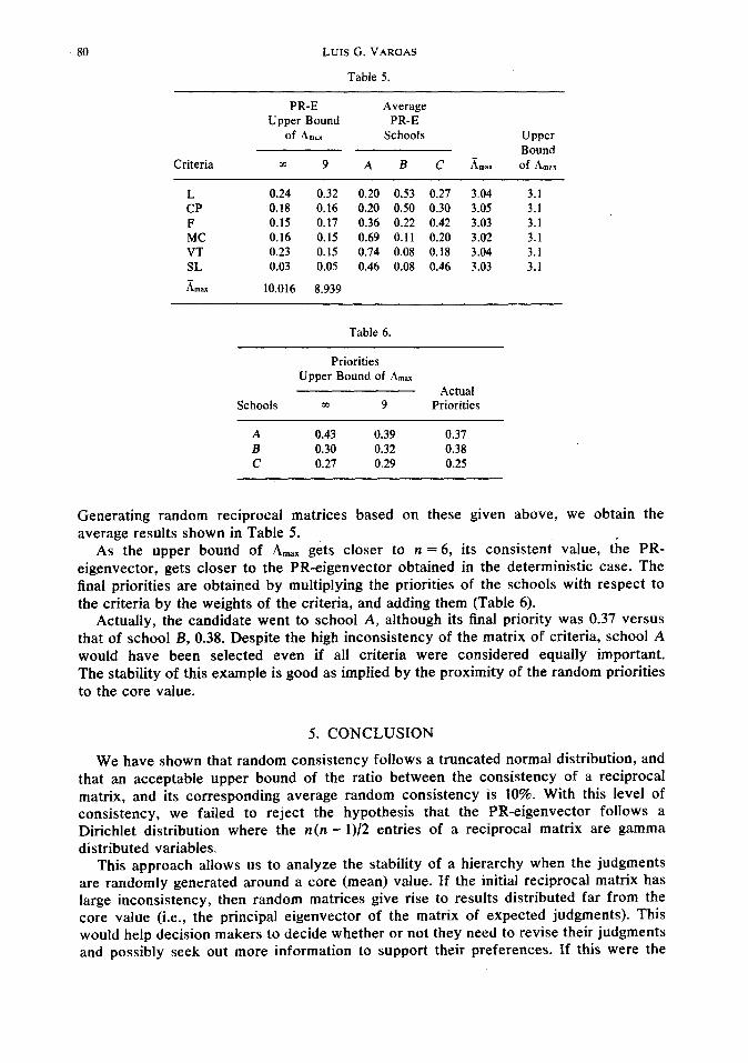
Table 5.

Criteria

PR-E Average Upper Bound PR-E

of Amax Schools Upper Bound

m 9 A B C ii,,, of Amx

L 0.24 0.32 0.20 0.53 0.27 3.04 3.1 CP 0.18 0.16 0.20 0.50 0.30 3.05 3.1 F 0.15 0.17 0.36 0.22 0.42 3.03 3.1 MC 0.16 0.15 0.69 0.11 0.20 3.02 3.1 VT 0.23 0.15 0.74 0.08 0.18 3.04 3.1 SL 0.03 0.05 0.46 0.08 0.46 3.03 3.1

Amax 10.016 8.939

Table 6.

Priorities Upper Bound of Am,

Actual Schools m 9 Priorities

A 0.43 0.39 0.37 B 0.30 0.32 0.38 c 0.27 0.29 0.25

Generating random reciprocal matrices based on these given above, we obtain the average results shown in Table 5.

As the upper bound of A,,, gets closer to n = 6, its consistent value, the PR- eigenvector, gets closer to the PR-eigenvector obtained in the deterministic case. The final priorities are obtained by multiplying the priorities of the schools with respect to the criteria by the weights of the criteria, and adding them (Table 6).

Actually, the candidate went to school A, although its final priority was 0.37 versus that of school B, 0.38. Despite the high inconsistency of the matrix of criteria, school A would have been selected even if all criteria were considered equally important. The stability of this example is good as implied by the proximity of the random priorities to the core value.

5. CONCLUSION

We have shown that random consistency follows a truncated normal distribution, and that an acceptable upper bound of the ratio between the consistency of a reciprocal matrix, and its corresponding average random consistency is 10%. With this level of consistency, we failed to reject the hypothesis that the PR-eigenvector follows a Dirichlet distribution where the n(n - 1)/2 entries of a reciprocal matrix are gamma distributed variables.

This approach allows us to analyze the stability of a hierarchy when the judgments are randomly generated around a core (mean) value. If the initial reciprocal matrix has large inconsistency, then random matrices give rise to results distributed far from the core value (i.e., the principal eigenvector of the matrix of expected judgments). This would help decision makers to decide whether or not they need to revise their judgments and possibly seek out more information to support their preferences. If this were the

Fkciprocal matrices with random coefficients 81

case, there are severai methods to improve consistency. For example, one could first elicit judgments regardless of their consistency, then rank-order the activities according to their prioritics, and obtain a new set of judgments.

On the other hand, if we restrict inconsistency in the random judgments through a rejection procedure of throwing out any matrix with inconsistency greater than IO%, the results obtained are close to the core value provided that the inconsistency of the matrix of expected judgments is less than or equal to 10%.

This is a particularly useful method for those situations where a limited amounted of information is available. Consider, for example, a committee entrusted by the mayor of a city to provide recommendations on several projects of interest to the community. Let us assume that the mayor intends to run for reelection, and is interested in increasing the number of constituents who would vote for for him. Let us also assume that some of the projects may create controversies and possibly decrease the mayor’s public image. How can he decide on what project to implement to maximize the number of votes?

The ideal, though impractical, situation would be to ask each voting member of the community to give his opinion about the desirability of each project. In this manner one could analyze the community’s preferences and couple them with the recommendations of the committee to reach a better rounded decision. In practice, this is usually accomplished through statistical sampling. However, to infer majority preferences from a sample carries along a measurement error. This error may be due in part to the fact that individual preferences depend on the state of mind of the individual and the information available to him. Hence, it seems as if preferences are in many cases spontaneous and momentary decisions rather than consequences of beliefs and experience.

The method proposed here attempts to infer as a “first-cut” from circulating in- formation average public preferences without having to survey opinions which as we said above may only reflect feelings at a given moment, Hence, in our example, the members of the committee could try to assess the preferences of the majority by asking questions such as given two projects, and given a criterion with respect to which the projects are compared, which one is more preferred by the community and how much? They would have to carry out a debate projecting how the community feels about the projects. The resulting judgments would be the core value or average preference of the community as estimated by the committee. Using the method of random reciprocal matrices we can compute the estimated relative preferences of the projects. These priorities along with the committee recommendations can be used to build firmer ground for the decision. Presumably interaction with members of the community would improve the surmised judgments.

Some areas in which the procedure could be applied are marketing decisions-to study the likelihood of success of new products; prediction of outcomes from conflicts- to analyze potential regions, issues, or events which could trigger conflicts; and political candidacy-to study issues on which a candidate must express an opinion, and analyze how his constituents would feel about the issues. Then, he could direct his attention to problems that could provide him with an advantage over the other candidates and bring him the majority of the votes.

We are carrying out work in these areas to develop specific applications to illustrate the approach in greater detail.

REFERENCES

1. Saaty. T. L. The Annlytic Hierarchy Process, McGraw-Hill International (1980). 2. Vargas, L. G., Analysis of sensitivity of reciprocal matrices. Appl. Math. Computat. (submitted).