Regularization Algorithms for Transition MatricesAlexander Kreinin and Marina Sidelnikova

Both estimating portfolio credit risk and pricing credit risky securities require transition matrices for arbitary time horizons. Simply computing the root of the annual transition matrix is unacceptable because the resulting matrices often contain negative elements. A similar situation exists when taking the logarithm of the annual transition matrix to compute a generator. This paper develops regularization algorithms for obtaining transition matrices and generators that give rise to close approximations of a given annual transition matrix. In our approach, the root or logarithm of the annual transition matrix is transformed, on a row-by-row basis, into a valid transition matrix or generator by projecting each row onto an appropriate set in a Euclidean space. Our methods compare favourably with other known regularization algorithms.

Credit risk models typically assume that, over time, a counterparty’s credit rating migrates among a set of possible credit states. Mathematically, this process can be modelled as a finite Markov chain, which assumes that the credit rating changes successively from one state to another, at given time intervals, with a certain probability. The probabilities of credit migration form a transition matrix. Annual transition matrices, which specify the probability of changing states over a one-year period, can be obtained from several agencies that specialize in credit data.

Risk management practices and the reduced form pricing of instruments are based on the finite Markov chain model. For example, Jarrow et al. (1997), Das and Tufano (1996), and Lando (2000) discuss the pricing and hedging of over the counter derivatives with counterparty risk and corporate debt with embedded options, relying on a Markov model of credit migration. For both continuous and discrete-time pricing models, knowledge of the annual transition matrix is insufficient for pricing since most instruments have maturities or cash flows that

occur on a non-annual basis. For example, pricing a credit risky instrument that matures in six months requires a six-month transition matrix. Thus, in general, we need to obtain transition matrices over arbitrary time horizons. Note that if the transition process is time homogeneous, then the n-period transition matrix can be obtained by simply raising the one-period transition matrix to the power n. Therefore, time homogeneity implies that a one-year transition matrix determines all transitions over any integer number of years.

Although this feature of the model is very attractive, it creates some conceptual problems. A six-month transition matrix, for example, should be a square root of the annual transition matrix. Unfortunately, this may not be possible; raising the annual transition matrix to a power less than one typically results in a matrix with negative elements, which is not a transition matrix. Moreover, even when it does exist, a six-month transition matrix may not be unique (see, e.g., Kingman 1962, Carette 1995). If a given annual transition matrix gives rise to several possible six-month transition matrices, the

23ALGO RESEARCH QUARTERLY VOL. 4, NOS.1/2 MARCH/JUNE 2001

Regularization algorithms

natural question is: Which matrix does one use for pricing purposes?

Thus, computing the fractional roots of an annual transition matrix is an ill-posed problem; the result may not be a valid transition matrix or it may not be unique. When faced with such a problem, one possibility is to reformulate it in a manner that allows it to be more readily solved. In this paper, we use this process, known as regularization, to obtain transition matrices for arbitrary time horizons that closely approximate the roots of an annual transition matrix.

One approach that obtains transition matrices for periods of arbitrary length involves embedding the discrete-time Markov chain into a continuous-time Markov process (Kingman 1962). For a continuous-time Markov process, any transition matrix (i.e., for a period of any length) can be expressed as the exponential of a so-called generator matrix. Thus, solving the embedding problem essentially allows one to find a generator that is consistent with the annual transition matrix of the discrete-time Markov chain. However, computing the generator of an existing transition matrix by taking its logarithm still raises the issues of existence and uniqueness. In fact, as we note in this paper, empirically observed transition matrices typically have properties that preclude the existence of a generator (see Israel et al. 2001). Alternatively, more than one generator may give rise to the same transition matrix (Kingman 1962, Carette 1995). To avoid these difficulties, the preferred approach is to estimate the generator directly and then use it to construct transition matrices as necessary. Unfortunately, agencies that provide data on credit migration deal with annualized transition matrices rather than with their generators.

There are a number of examples of using generators for pricing credit risky instruments. In Jarrow et al. (1997), Das and Tufano (1996) and Lando (2000), the discrete-time and continuous-time arbitrage-free models assume the existence and uniqueness of an equivalent martingale measure. To construct this measure in the framework of Markov credit migration models, one has to determine the risk-neutral transition

probabilities from market prices and historical transition probabilities. Thus, one must consider the conditions that guarantee uniqueness of the equivalent martingale measure. The framework suggested by Jarrow et al. (1997) and Das and Tufano (1996) simply assumes the existence of a generator matrix governing credit migration. In Lando (1999), however, the generator is computed from the transition matrix, which potentially raises the issue of uniqueness. If the generator of a transition matrix is not unique then, from a pricing perspective, this may lead to arbitrage. Therefore, the arbitrage-free approach should ideally be based on estimating the generator directly, as in Jarrow et al. (1997) and Lando (2000).

In this paper, we also present a regularization algorithm for computing the generator that can be used for the best approximation of a given transition matrix. Thus, we provide a means to obtain either a root of a transition matrix for discrete-time credit risk models or a generator for continuous-time models. Using our approach, one finds the transition matrix or generator that is closest, in a Euclidean distance sense, to the given root or logarithm, respectively, of the annual transition matrix.

This paper is organized as follows. The first section provides relevant background material. It reviews Markov chains and transition matrices in the context of credit models. The next section describes the embedding problem that is closely related to the regularization of transition matrices. Then, we discuss the issue of uniqueness and examine the properties of a typical transition matrix. In the next section we formulate regularization problems for the root and generator matrices and present algorithms for their solution. We illustrate the regularization procedures by finding a six-month transition matrix and then we compare them on a broader sample of transition matrices. The final section contains our conclusions and suggestions for further research.

Markov chains and transition matrices

A finite Markov chain in discrete time S(t), t = 0, 1, 2, ..., is defined by the following elements:

24ALGO RESEARCH QUARTERLY MARCH/JUNE 2001

Regularization algorithms

• A finite set of states

• An initial probability distribution,

satisfying and

• A family of transition matrices , where

. The transition probabilities satisfy

(1)

We say that the Markov chain S(t) is time homogeneous if the transition probabilities do not depend on t, that is,

.

In credit risk modelling, a one-year transition matrix is the only source of information regarding the transition probabilities. Furthermore, rating agencies do not provide time-dependent forecasts of transition matrices.1 For these reasons, it is practical to assume a time-homogeneous Markov chain when simulating credit events. Note that this also allows the above notation to be simplified: we denote a one-period transition matrix by and, more generally, a t-period (i.e., for the time interval [0, t]) transition matrix by .

The transition probabilities satisfy the relation

or, in matrix form, . The latter formula, usually called the semi-group property, implies

(2)

It is easily verified that any integer power of a

transition matrix is a transition matrix as well. From Equation 2, it follows that the probability distribution of the Markov chain at time t satisfies

where

.

Regular Credit Migration Model

Finite Markov chains used in credit risk models have one special state that represents a default event. This state is absorbing; once reached, the chain will remain there indefinitely. In what follows, we assume that the default state is numbered n. Then we have

and for all ,

To distinguish from the more general case described in the previous section, we define a regular credit migration model (RCMM) to be a Markov chain that also satisfies the following three properties:

• There is one and only one absorbing state.

• There exists such that for all .

• The determinant of the annual transition matrix A is not equal to zero, and the eigenvalues are distinct (this allows us to compute the logarithm of A).

Empirically, we observe that values are common. Thus, even a counterparty with the highest credit rating has a positive probability of defaulting within two to five years. Furthermore, for an RCMM, the transition matrix A(t) satisfies (Snell 1988)

(3)

where

S 1 2 … n, , ,{ }=

q 0( ) P S 0( ) 1={ } P S 0( ) 2={ } … P S 0( ) n={ },,( )=P S 0( ) i={ } 0 i,≥ 1 2 … n, , ,=

P S 0( ) i={ }i 1=

n

� 1=

A t t 1+,( ) aij t t 1+,( )=

aij t t 1+,( ) P S t 1+( ) j S t( ) i=={ }=

aij

j 1=

n

� t t 1+,( ) 1= for i 1 2 …n, ,=

aij t t, 1+( ) 0≥ for i j, 1 2 …n, ,=

aij t t 1+,( ) aij 0 1,( ) aij= =

A aij=

A t( ) aij t( )=

aij t( )

aij t( ) aik m( )akj t m–( )k 1=

n

�= , m 1 2 … t 1–, , ,=

A t( ) A m( )A t m–( )=

A t( ) At=

q t( ) q 0( )At=

q t( ) P S t( ) 0={ } P S t( ) 1={ } … P S t( ) n={ }, , ,( )=

ann t( ) 1= anj t( ) 0= j n≠ t 1 2 …, ,=

tP 1≥ ain tP( ) 0>

i 1 2 … n, , ,=

2 tP 5≤ ≤

A t( ) D as t ∞→→

D

0 0 … 0 10 0 … 0 1… … … … …0 0 … 0 1

=

25ALGO RESEARCH QUARTERLY MARCH/JUNE 2001

Regularization algorithms

Equation 3 implies that default will eventually occur regardless of the initial credit rating; the default state is accessible from every credit state. However, the average time to default may be very large for some initial credit states.

Analysis of empirical annual transition matrices indicates that the diagonal probabilities, aii, dominate in corresponding rows (i.e., for

). However, this relation is not satisfied for arbitrary time t > 1, as is apparent from the matrix D in Equation 3, for example. For this reason, we do not include this condition in the definition of an RCMM and are unable to use the properties of diagonally dominant matrices in our analysis.

Embedding problem

Computation of the fractional roots of transition matrices is closely related to the embedding problem of Markov chains. Given a finite Markov chain in discrete time, S(t), the embedding problem can be posed as follows:

Is it possible to construct a Markov process

in continuous time such that the

probability distribution of at time is identical to the distribution of ?

The embedding problem was studied by Kingman (1962), Carette (1995), Iwanik and Shiflett (1986), and Frydman (1983). The main approach developed in these papers is based on the notion of the generator of a Markov process.

A generator is a matrix G whose elements satisfy

(4)

Generators form a semi-group in the space of matrices, which means that the sum of two generators is also a generator. Note that if A is a transition matrix then A – I is a generator, where I is the identity matrix of the same dimensions as A. Moreover, if G is a generator then eG is a transition matrix (Snell 1988).

Let denote the transition matrix of the

Markov process . The matrix is

called the generator of if satisfies

In this case, we obtain

Therefore, if the distribution of the Markov

process is identical to that of the Markov chain S(t) at time then the transition matrix A must satisfy

(5)

If the matrix exists and is unique, then one

can define a continuous-time extension, , of the transition matrix A as follows

(6)

Note that since τ is continuous, Equation 6 allows us to obtain a transition matrix for a period of arbitary length.

While we can calculate from Equation 5, there is no guarantee that the matrix ln(A) satisfies Equation 4. In general, the question of when a transition matrix A can be represented in the form A = eG, where G is a generator, is technically very difficult. There are several known results related to this problem. For 2 × 2 transition matrices, the generator exists if the determinant of the matrix is positive (see, e.g., Kingman 1962). However, for the 3 × 3 case, studied by Iwanik and Shiflett (1986) and Frydman (1983), no general conditions were found for the existence of the generator. Note that for transition matrices of arbitrary dimensions, inferring such existence conditions from the characterization of their eigenvalues (see, e.g., Karpelevitch 1951) is an interesting possibility.

Finally, we note that the problem of computing

aii aij>

i j≠

S τ( ) τ 0≥,{ } τ

S τ( ) τ 1 2 …, ,=S τ( )

gij

j 1=

n

� 0= for i 1 2 …n ,, ,=

gi j 0≥ for i j, 1 2 …n and i j.≠, ,=

A τ( )

S τ( ) G gi j=

S τ( ) A τ( )

τdd A AG=

A τ( ) eτ G τ 0>,=

S τ( )τ 1 2 …, ,=

A eG=

G

A τ( )

A τ( ) eτ G=

G A( )ln=

26ALGO RESEARCH QUARTERLY MARCH/JUNE 2001

Regularization algorithms

the logarithm and exponential of a matrix is nontrivial (Moler and Van Loan 1978 and Dieci 1996) and a detailed discussion is beyond the scope of this paper. Our implementation is based on Schur decomposition and the Parlett method (Moler and Van Loan 1978).

Non-uniqueness problem

In this section, we address the problem of non-uniqueness of the resulting transition matrix when one computes credit transition probabilities over time horizons of less than one year. We start with an instructive example that demonstrates the non-uniqueness effect. Consider the family of transition matrices

Let us impose the condition px = a, where 0 < p < 1 and 0 < x < 1. Then, the annual transition matrix, is

However, there exists another transition matrix A*(0.5) that is also the square root of A:

Note that A*(0.5) is the solution that would be obtained using a generator, as discussed in the previous section.

This example demonstrates that there can be infinitely many square roots of the transition matrix, each of which has its own financial

interpretation. It is, therefore, natural to ask: What conditions guarantee the uniqueness the resulting transition matrix? A partial answer to this question can be found in Theorem 1 and Theorem 2 below, from the paper by Israel et al. (2001).

Theorem 1: Suppose that all diagonal elements

dominate in the transition matrix A (i.e., ).

Then the eigenvalues of A belong to the disc in the complex plane, and the Taylor series

expansion for the logarithm of the transition matrix converges geometrically quickly to a real matrix, Q, that satisfies exp(Q) = A. Furthermore, under this condition, the transition matrix can have, at most, one generator: if a generator exists, then it is unique.

Note that Theorem 1 does not say that diagonal dominance guarantees existence of the generator. In our analysis of 32 empirical transition matrices, only 10 had dominant diagonal elements and, among those, only one matrix had a generator.

Theorem 2 uses the following definition: a state j is accessible from a state i if there is a sequence of states such that

Theorem 2: Suppose that the transition matrix, A, satisfies one of the conditions.

(1) det A < 0,

(2) det A >

(3) there are states i and j such that j is accessible from i, but aij = 0

Then there does not exist an exact generator for A.

A 0.5( )

0 p … 0 0 1 p–x 0 … 0 0 1 x–

… … … … … …0 0 … 0 p 1 p–0 0 … x 0 1 x–0 0 … 0 0 1

=

A A 0.5( ) A 0.5( )⋅=

A

a 0 0 … 0 1 a–0 a 0 … 0 1 a–0 0 a … 0 1 a–… … … … … …0 0 0 … a 1 a–0 0 0 … 0 1

=

A* 0.5( )

a 0 … 0 1 a–0 a … 0 1 a–… … … … …

0 0 … a 1 a–0 0 … 0 1

=

aii12-->

λ 1– 1≤

k0 i= k1 k2 …, , , km j=

aklkl 1+

l 0=

m 1–

∏ 0>

aii

i 1=

n

∏

27ALGO RESEARCH QUARTERLY MARCH/JUNE 2001

Regularization algorithms

The first and the second conditions of Theorem 2 were not satisfied by any of the 32 empirical transition matrices we examined, while the third condition was satisfied in the majority of the cases. There is a natural explanation of why the third condition should be satisfied by an RCMM. Usually, the one-year transition probability from the highest credit grade to default is zero. However, the default state is accessible from any credit state of the transition matrix. Therefore, we can conclude that, in the majority of practical cases, an exact generator does not exist. However, we can also not deny the possibility of an annual transition matrix having several generators, which can lead potentially to arbitrage when pricing credit risky securities.

Example of a transition matrix

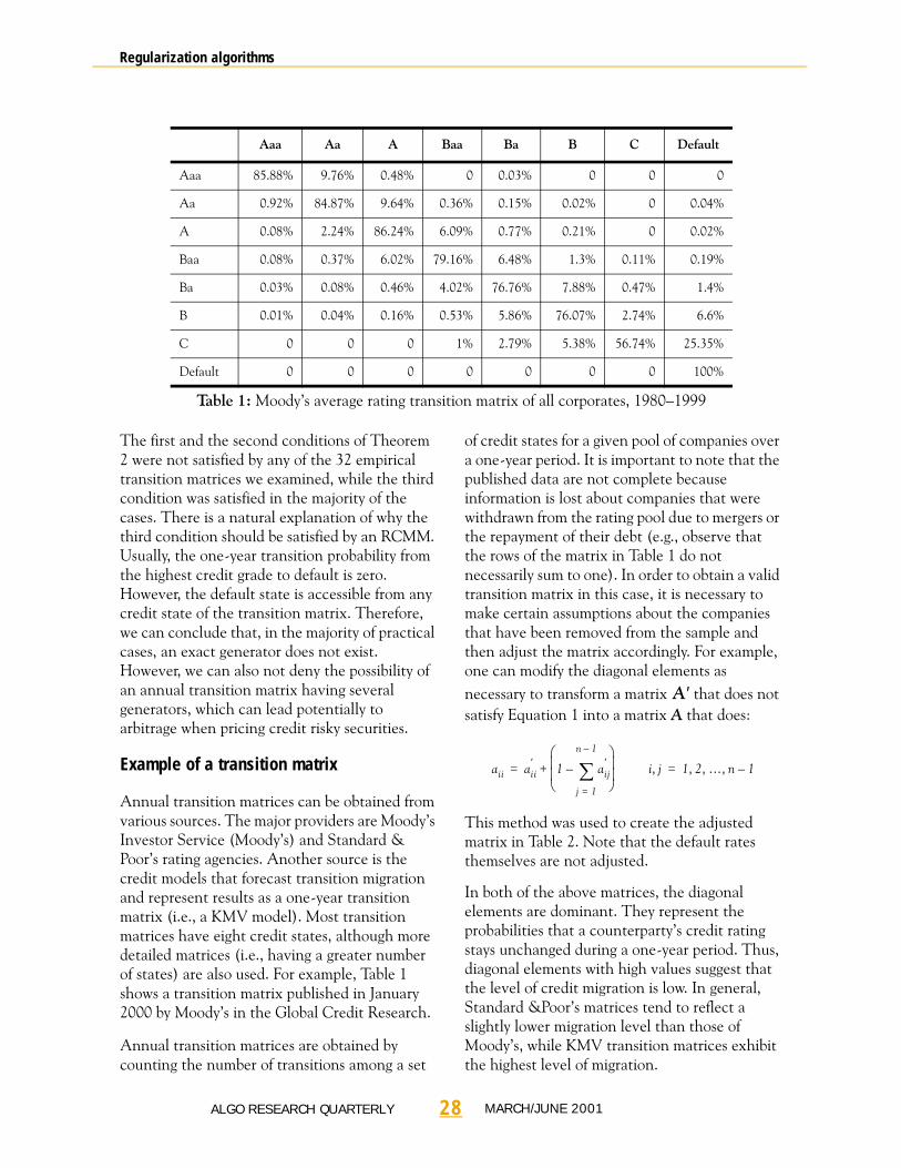
Annual transition matrices can be obtained from various sources. The major providers are Moody’s Investor Service (Moody’s) and Standard & Poor’s rating agencies. Another source is the credit models that forecast transition migration and represent results as a one-year transition matrix (i.e., a KMV model). Most transition matrices have eight credit states, although more detailed matrices (i.e., having a greater number of states) are also used. For example, Table 1 shows a transition matrix published in January 2000 by Moody’s in the Global Credit Research.

Annual transition matrices are obtained by counting the number of transitions among a set

of credit states for a given pool of companies over a one-year period. It is important to note that the published data are not complete because information is lost about companies that were withdrawn from the rating pool due to mergers or the repayment of their debt (e.g., observe that the rows of the matrix in Table 1 do not necessarily sum to one). In order to obtain a valid transition matrix in this case, it is necessary to make certain assumptions about the companies that have been removed from the sample and then adjust the matrix accordingly. For example, one can modify the diagonal elements as necessary to transform a matrix that does not satisfy Equation 1 into a matrix A that does:

This method was used to create the adjusted matrix in Table 2. Note that the default rates themselves are not adjusted.

In both of the above matrices, the diagonal elements are dominant. They represent the probabilities that a counterparty’s credit rating stays unchanged during a one-year period. Thus, diagonal elements with high values suggest that the level of credit migration is low. In general, Standard &Poor’s matrices tend to reflect a slightly lower migration level than those of Moody’s, while KMV transition matrices exhibit the highest level of migration.

Aaa Aa A Baa Ba B C Default

Aaa 85.88% 9.76% 0.48% 0 0.03% 0 0 0

Aa 0.92% 84.87% 9.64% 0.36% 0.15% 0.02% 0 0.04%

A 0.08% 2.24% 86.24% 6.09% 0.77% 0.21% 0 0.02%

Baa 0.08% 0.37% 6.02% 79.16% 6.48% 1.3% 0.11% 0.19%

Ba 0.03% 0.08% 0.46% 4.02% 76.76% 7.88% 0.47% 1.4%

B 0.01% 0.04% 0.16% 0.53% 5.86% 76.07% 2.74% 6.6%

C 0 0 0 1% 2.79% 5.38% 56.74% 25.35%

Default 0 0 0 0 0 0 0 100%

Table 1: Moody’s average rating transition matrix of all corporates, 1980–1999

A ′

aii ai i′ 1 aij

′

j 1=

n 1–

�–� �� �� �� �

+= i j, 1 2 … n 1–, , ,=

28ALGO RESEARCH QUARTERLY MARCH/JUNE 2001

Regularization algorithms

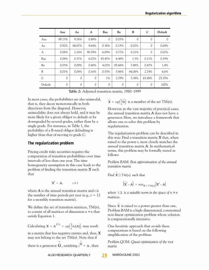
In most cases, the probabilities are also unimodal, that is, they decay monotonically in both directions from the diagonal. However, unimodality does not always hold, and it may be more likely for a given obligor to default or be downgraded by several grades, rather than by a single grade. For instance, in Table 1, the probability of a B-rated obligor defaulting is higher than that of moving to grade C.

The regularization problem

Pricing credit risky securities requires the computation of transition probabilities over time intervals of less than one year. The time homogeneity assumption in this case leads to the problem of finding the transition matrix X such that

where A is the annual transition matrix and t is the number of time periods per year (e.g., t = 12 for a monthly transition matrix).

We define the set of transition matrices, TM(n), to consist of all matrices of dimension n × n that satisfy Equation 1.

Calculating may result

in a matrix that has negative entries and, thus, X may not belong to the set TM(n). Note that if

there is a generator , satisfying , then

is a member of the set TM(n).

However, in the vast majority of practical cases, the annual transition matrix A does not have a generator. Here, we introduce a framework that allows one to solve this problem by regularization.

The regularization problem can be described in this way: Find a transition matrix X that, when raised to the power t, most closely matches the annual transition matrix A. In mathematical terms, this problem may be formally stated as follows:

Problem BAM: Best approximation of the annual transition matrix

Find such that

where is a suitable norm in the space of n × n matrices.

Since is raised to a power greater than one, Problem BAM is a high-dimensional, constrained non-linear optimization problem whose solution is computationally intensive.

One heuristic approach that avoids these computations is based on the following simplification of the problem:

Problem QOM: Quasi-optimization of the root matrix

Aaa Aa A Baa Ba B C Default

Aaa 89.73% 9.76% 0.48% 0 0.03% 0 0 0

Aa 0.92% 88.87% 9.64% 0.36% 0.15% 0.02% 0 0.04%

A 0.08% 2.24% 90.59% 6.09% 0.77% 0.21% 0 0.02%

Baa 0.08% 0.37% 6.02% 85.45% 6.48% 1.3% 0.11% 0.19%

Ba 0.03% 0.08% 0.46% 4.02% 85.66% 7.88% 0.47% 1.4%

B 0.01% 0.04% 0.16% 0.53% 5.86% 84.06% 2.74% 6.6%

C 0 0 0 1% 2.79% 5.38% 65.48% 25.35%

Default 0 0 0 0 0 0 0 100%

Table 2: Adjusted transition matrix, 1980–1999

Xt A,= t 1>

X A1 t⁄ 1

t-- A( )ln� �� �exp= =

G eG

A=

X 1t--G� �� �exp=

X TM n( )∈

Xt

A– minX TM n( )∈ Xt A–=

⋅

X

29ALGO RESEARCH QUARTERLY MARCH/JUNE 2001

Regularization algorithms

Find such that

Thus, problem QOM finds the transition matrix that is as close as possible to the fractional root of the annual transition matrix, as given by

. Comparing problems BAM

and QOM suggests that and should be close to each other; for this reason, it is natural to call

a quasi-solution to problem BAM.

The second heuristic approach uses the generator as the object of regularization. First, define the set of generator matrices, G(n), consisting of all matrices of dimension n × n that satisfy Equation 4. Consider the problem:

Problem QOG: Quasi-optimization of the generator

Find such that

Problems BAM and QOG are related under the

assumption that exp( ) is close to , and thus

the matrix can also be viewed as a quasi-solution to problem BAM. Again, problem QOG is much more attractive than problem BAM in a computational sense.

Figure 1 illustrates the relationships among the above three problems.

Figure 1: Relationship of problems BAM, QOM and QOG

When A1/t is not a valid transition matrix, problems BAM and QOM find solutions in TM(n) that are as close as possible to the root matrix. Similarly, when ln(A) is not a valid generator, problem QOG finds the closest

possible generator matrix . Exponentiation of the generator then yields a valid transition matrix that is close to A1/t.

Solving the quasi-optimization problems

In this section, we present fast algorithms for solving problems QOM and QOG.

Solving problem QOM

To solve problem QOM, we use the fact that the set of transition matrices, TM(n), can be represented as a Cartesian product of n identical n-dimensional simplices. That is, each row of the transition matrix satisfies Equation 1 and thus it belongs to the n-dimensional simplex, Sim(n), defined as follows:

(7)

Furthermore, note that Sim(n) is contained in the hyperplane H(n)

Suppose that we use the Euclidean norm to measure the distance between any two points x and y in Rn:

Then problem QOM can essentially be solved on

a row-by-row basis by projecting a point

(i.e., a row of the matrix ) onto the simplex defined in Equation 7. That is, problem QOM can be reduced to n independent instances of the following distance minimization problem:

Xˆ

TM n( )∈

Xˆ

A1 t⁄– minX TM n( )∈ X A1 t⁄–=

A1 t⁄ 1t-- A( )ln� �� �exp=

Xˆ

X

Xˆ

Gˆ

G n( )∈

Gˆ

A( )ln– minX G n( )∈ X A( )ln–=

1t--G

ˆX

Gˆ

TM(n)

X

G(n)

Problem QOM

Problem QOG

A1/t

ln (A)

X~

^

G^

Problem BAM

exp(1/t G)

Gˆ

Sim n( ) x1 … xn, ,( ) Rn∈ xi

i 1=

n

� 1 xi 0≥,=,

� � � �

=

H n( ) x1 … xn, ,( ) Rn∈ xi

i 1=

n

� 1=,

� � � �

=

dist x y,( ) yi xi–( )2

i 1=

n

�= , x y, Rn∈

a Rn∈

A1 t⁄

30ALGO RESEARCH QUARTERLY MARCH/JUNE 2001

Regularization algorithms

Problem DMPM: Distance minimization problem for the root matrix

For a given point , , find

such that

To the best of our knowledge, an algorithm for solving problem DMPM has not been previously published. The following algorithm was suggested in Merkoulovitch (2000), where the geometrical proof of convergence is given.

Step 1. Find the projection b of the point a on the hyperplane H(n): set , where

Step 2. If all the coordinates of b are non-negative then stop; b is the solution to problem DMPM.

Step 3. Let , where π is a permutation that orders the coordinates of b in descending sequence.

Step 4. Compute for

k = 1, 2,..., n. The sums Ck satisfy

0 ≤ C1 ≤ C2 ≤ ... ≤ Cn.

Step 5. Find k* = max{k: k ≥ 1, Ck ≤ 1}.

Step 6. Construct the vector as

follows. For all j > k* set , and for j ≤ k* set

Step 7. Apply the inverse permutation π-1 to ;

is the solution to problem DMPM.

The correctness of the algorithm above follows from the geometrical proof in Merkoulovitch (2000) and from analytical arguments in Tuenter (2000). While a detailed proof is beyond the

scope of this paper, it relies on the following key propositions.

Proposition 1: Let a = (a1, ..., an) be the initial point

and let be the optimal solution to problem DMPM. Then if , then

.

Proposition 1 states that the elements of the optimal solution are ordered in the same sequence as those of the initial point. This allows us to consider only the case where the coordinates of a are ordered, without loss of generality.

Proposition 2: If b is the projection of a on H(n) and bk < 0 some k, then = 0 for j = k, ..., n.

Proposition 2 states that, if after projection on the hyperplane, some of the coordinates are negative, then, in the optimal solution these coordinates equal zero. This allows us to reduce the original problem to a discrete optimization problem as follows.

With λ obtained as in Step 1 of the algorithm,

define the function for

l = 1, 2, ..., n (note that for k < m).

The solution of the distance minimization problem can be obtained from solving:

The solution l* to this problem determines the optimal number of coordinates k* to be equal to zero in Step 5.

Proposition 3: The objective function f(l) is monotonic (i.e., f(l) > f(l + 1)).

Proposition 3 follows from the identity

a Rn∈ a a1 …an( , )=

x∗ Sim n( )∈

dist a x∗,( ) minx Sim n( )∈ dist a x,( )=

bi ai λ–=

λ 1n-- ai

i 1=

n

� 1–� �� �� �� �

=

a π b( )=

Ck ai

i 1=

k

� k ak⋅–=

x Sim n( )∈

xj 0=

xj aj1k∗----- 1 ai

i 1=

k∗

�–� �� �� �� �

+=

x

π 1– x( )

x∗ x1∗ … x, n

∗,( )=

a1 … an≥ ≥

x1∗ … xn

∗≥ ≥

xj∗

f l( ) l λ2⋅ ai2

i l 1+=

n

�+=

ai2

i k=

m

� 0≡

min f l( )s.t.

l λ⋅ ai

i 1=

l

�+ 1=

λ al+ 0≥ , l = 1, ..., n

l Z+∈

31ALGO RESEARCH QUARTERLY MARCH/JUNE 2001

Regularization algorithms

where

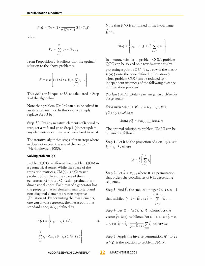
From Proposition 3, it follows that the optimal solution to the above problem is

This yields an l* equal to k*, as calculated in Step 5 of the algorithm.

Note that problem DMPM can also be solved in an iterative manner. In this case, we simply replace Step 3 by:

Step . Fix any negative elements of b equal to zero, set a = b and go to Step 1 (do not update any elements once they have been fixed to zero).

The iterative algorithm stops after m steps where m does not exceed the size of the vector a (Merkoulovitch 2000).

Solving problem QOG

Problem QOG is different from problem QOM in a geometrical sense. While the space of the transition matrices, TM(n), is a Cartesian product of simplices, the space of their generators, G(n), is a Cartesian product of n-dimensional cones. Each row of a generator has the property that its elements sum to zero and non-diagonal elements are non-negative (Equation 4). By permuting the row elements, one can always represent them as a point in a standard cone, , defined by

(8)

Note that K(n) is contained in the hyperplane

:

In a manner similar to problem QOM, problem QOG can be solved on a row-by-row basis by

projecting a point (i.e., a row of the matrix ) onto the cone defined in Equation 8.

Thus, problem QOG can be reduced to n independent instances of the following distance minimization problem:

Problem DMPG: Distance minimization problem for the generator

For a given point , , find

such that

The optimal solution to problem DMPG can be obtained as follows:

Step 1. Let b be the projection of a on : set , where

Step 2. Let , where π is a permutation that orders the coordinates of b in descending sequence.

Step 3. Find l*, the smallest integer 2 ≤ l ≤ n – 1

that satisfies .

Step 4. Let . Construct the

vector as follows. For all set ,

and set otherwise.

Step 5. Apply the inverse permutation π–1 to ;

is the solution to problem DMPM.

f m( ) f m 1+( ) 1m m 1+( )⋅--------------------------- 1 Tm–( )2⋅+=

Tm ai

i 1=

m

� m am 1+⋅–=

l∗ max l : 1 l n≤ ≤ lal ai

i 1=

l

� 1–≥,

� � � �

=

3 ′

K n( )

K n( ) x1 … xn, ,( ) Rn ,∈

xi

i 1=

n

� 0 x1 0 xi 0 for i 2≥,≥,≤,=

�

�

�

�

=

Hˆ

n( )

Hˆ

n( ) x1 … xn, ,( ) Rn∈ xi

i 1=

n

� 0=,

� � � �

=

a Rn∈A( )ln

a Rn∈ a a1 …an( , )=

g∗ K n( )∈

dist a g∗,( ) ming K n( )∈ dist a g,( )=

Hˆ

n( )bi ai λ–=

λ 1n-- ai

i 1=

n

�� �� �� �� �

=

a π b( )=

n l– 1+( )al 1+ a1 an i–

i 0=

n l 1+( )–

�+≥

ℑ i: 2 i l*≤ ≤{ }=

g K n( )∈ i ℑ∈ gi 0=

gi aiˆ 1

n l∗ 1+–( )--------------------------- aj

ˆ

j ℑ∉�–=

g

π 1– g( )

32ALGO RESEARCH QUARTERLY MARCH/JUNE 2001

Regularization algorithms

The correctness of the above algorithm can be proved in a manner similar to that for the case of DMPM. An iterative implementation is possible in this case as well.

Other regularization methods for generators

In this section, we describe regularization methods suggested by Stromquist (1996) and Araten and Angbazo (1997). These methods adjust the matrix G = ln(A), the logarithm of the annual transition matrix, in order to construct a

generator . To satisfy Equation 6, all negative non-diagonal elements of G are first set to zero, and then selected elements are adjusted to ensure that each row sums to zero. Two such methods are diagonal adjustment (DA), which modifies only the diagonal elements, and weighted adjustment (WA), which modifies all

non-zero elements. The computation of proceeds as follows:

Step 1. Set for

i, j = 1, 2, ..., n.

Step 2a (diagonal adjustment). Set the diagonal elements to the negative sum of the non-diagonal elements:

or

Step 2b (weighted adjustment). Adjust the non-zero elements according to their relative magnitudes:

Example: a six-month transition matrix

We now illustrate the regularization algorithms by calculating a six-month transition matrix based on the annual transition matrix (A) in Table 2. Observe that A1/2, the square root of the annual transition matrix, contains negative elements (Table 3) and so it is not a valid transition matrix.

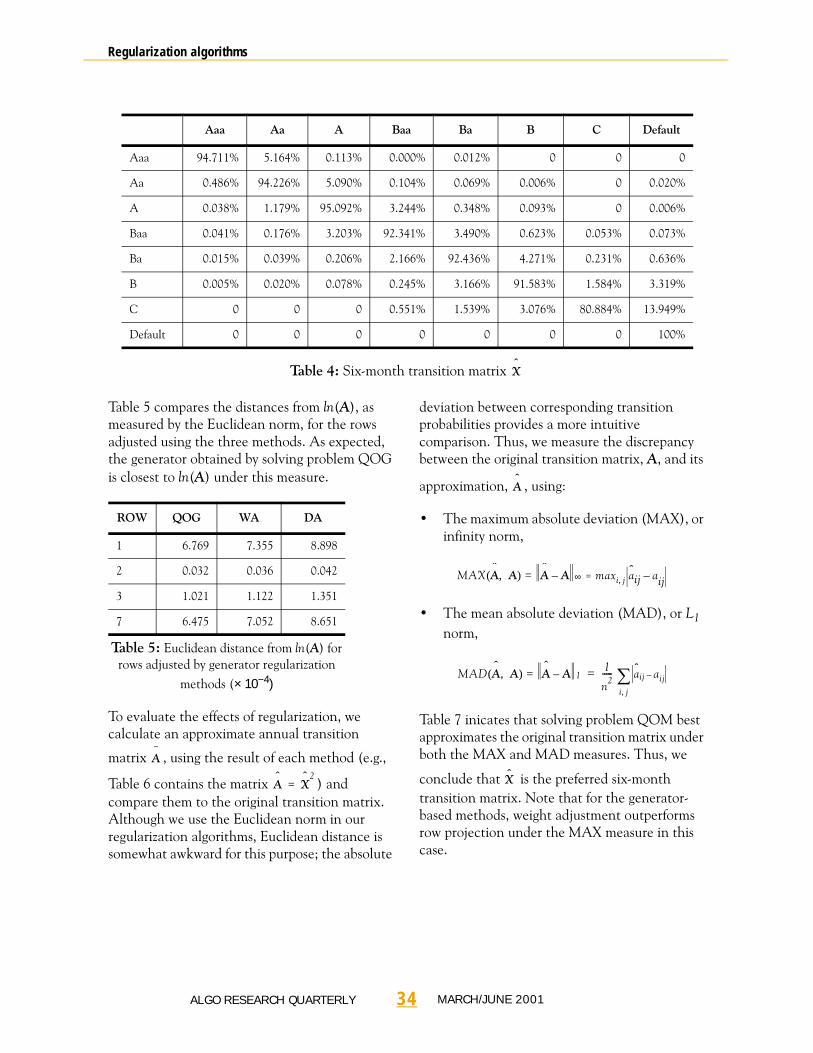
Table 4 shows , the transition matrix that is as close as possible to A1/2, which we obtain by solving problem QOM with the iterative row

projection algorithm. Note that all elements of are non-negative.

We also compute generators that approximate

ln(A) by solving problem QOG, and with the DA and WA methods. When computing the generator in this case, it is necessary to adjust only four of the eight rows comprising ln(A).

Aaa Aa A Baa Ba B C Default

Aaa 94.713% 5.164% 0.114% –0.005% 0.014% –0.001% –0.000% –0.001%

Aa 0.486% 94.226% 5.090% 0.104% 0.069% 0.006% 0.000% 0.020%

A 0.038% 1.179% 95.092% 3.244% 0.348% 0.094% -0.002% 0.006%

Baa 0.041% 0.176% 3.203% 92.341% 3.490% 0.623% 0.053% 0.073%

Ba 0.015% 0.039% 0.205% 2.166% 92.436% 4.271% 0.231% 0.636%

B 0.005% 0.020% 0.078% 0.245% 3.166% 91.583% 1.584% 3.319%

C 0.000% –0.001% –0.013% 0.554% 1.542% 3.079% 80.887% 13.952%

Default 0 0 0 0 0 0 0 100%

Table 3: Square root of Moody’s transition matrix (1999)

Gˆ

Gˆ

gi j0 if i j≠( ) and gij 0<

gij otherwise��

=

gi i gi j

j 1 j i≠,=

n

� for i = 1, 2, ..., n–=

gi j gi j gi j

gi j

j 1=

n

�

gi j

j 1=

n

�

----------------- for i, j = 1, 2, ..., n–=

Xˆ

Xˆ

33ALGO RESEARCH QUARTERLY MARCH/JUNE 2001

Regularization algorithms

Table 5 compares the distances from ln(A), as measured by the Euclidean norm, for the rows adjusted using the three methods. As expected, the generator obtained by solving problem QOG is closest to ln(A) under this measure.

To evaluate the effects of regularization, we calculate an approximate annual transition

matrix , using the result of each method (e.g.,

Table 6 contains the matrix ) and compare them to the original transition matrix. Although we use the Euclidean norm in our regularization algorithms, Euclidean distance is somewhat awkward for this purpose; the absolute

deviation between corresponding transition probabilities provides a more intuitive comparison. Thus, we measure the discrepancy between the original transition matrix, A, and its

approximation, , using:

• The maximum absolute deviation (MAX), or infinity norm,

• The mean absolute deviation (MAD), or L1 norm,

Table 7 inicates that solving problem QOM best approximates the original transition matrix under both the MAX and MAD measures. Thus, we

conclude that is the preferred six-month transition matrix. Note that for the generator-based methods, weight adjustment outperforms row projection under the MAX measure in this case.

Aaa Aa A Baa Ba B C Default

Aaa 94.711% 5.164% 0.113% 0.000% 0.012% 0 0 0

Aa 0.486% 94.226% 5.090% 0.104% 0.069% 0.006% 0 0.020%

A 0.038% 1.179% 95.092% 3.244% 0.348% 0.093% 0 0.006%

Baa 0.041% 0.176% 3.203% 92.341% 3.490% 0.623% 0.053% 0.073%

Ba 0.015% 0.039% 0.206% 2.166% 92.436% 4.271% 0.231% 0.636%

B 0.005% 0.020% 0.078% 0.245% 3.166% 91.583% 1.584% 3.319%

C 0 0 0 0.551% 1.539% 3.076% 80.884% 13.949%

Default 0 0 0 0 0 0 0 100%

Table 4: Six-month transition matrix Xˆ

ROW QOG WA DA

1 6.769 7.355 8.898

2 0.032 0.036 0.042

3 1.021 1.122 1.351

7 6.475 7.052 8.651

Table 5: Euclidean distance from ln(A) for rows adjusted by generator regularization

methods (× 10−4)

Aˆ

Aˆ

Xˆ 2

=

Aˆ

MAX Aˆ

A( , ) Aˆ

A–= ∞ maxi j, aij aij–=

MAD Aˆ

A( , ) Aˆ

A–= 11

n2----- aij ai j–

i j,�=

X

34ALGO RESEARCH QUARTERLY MARCH/JUNE 2001

Regularization algorithms

Robustness of regularization methods

We now briefly examine the robustness of the proposed regularization methods. Specifically, we consider the question: When solving problems QOM and QOG, do similar annual transition matrices give rise to similar six-month transition matrices?

For purposes of this example, we construct a perturbed matrix from the annual transition matrix A by setting

for i, j = 1, 2, ..., n, where uij is a uniformly distributed random variable from the interval [0.99, 1.01]. We then compute six-month

transition matrices and from by

solving problems QOM and QOG, respectively, and measure the deviations between the original and perturbed matrices.

Table 8 reports the results of 1,000 repetitions of the above experiment. Based on these results, we conclude that the regularization methods are robust with respect to small changes in the annual transition matrix.

Computational experiments

We now compare the performance of the regularization methods on a set of 32 annual transition matrices obtained from various sources. The sample includes:

• seventeen matrices of dimension 8 × 8 from Standard & Poor’s the period 1981–1997

• one 18 × 18 matrix from Standard & Poor’s for 1999

• one matrix of dimension 8 × 8 from Moody’s for 1999

• four 8 × 8 matrices from CreditMetrics

Aaa Aa A Baa Ba B C Default

Aaa 89.73% 9.76% 0.48% 0.01% 0.03% 0.00% 0.00% 0.00%

Aa 0.92% 88.87% 9.64% 0.36% 0.15% 0.02% 0.00% 0.04%

A 0.08% 2.24% 90.59% 6.09% 0.77% 0.21% 0.00% 0.02%

Baa 0.08% 0.37% 6.02% 85.45% 6.48% 1.30% 0.11% 0.19%

Ba 0.03% 0.08% 0.46% 4.02% 85.66% 7.88% 0.47% 1.40%

B 0.01% 0.04% 0.16% 0.53% 5.86% 84.06% 2.74% 6.60%

C 0.00% 0.00% 0.02% 1.00% 2.78% 5.37% 65.48% 25.34%

Default 0 0 0 0 0 0 0 100%

Table 6: Approximate annual transition matrix Aˆ

Xˆ 2

=

QOM QOG WA DA

MAX 2.320 4.599 4.544 6.341

MAD 0.131 0.382 0.395 0.404

Table 7: Differences between original (A)

and approximate ( ) annual transition matrix (× 10−4)

Aˆ

A ′

aij′ aijuij( ) aijui j( )

j 1=

n

�� �� �� �� �

1–

=

X′ 12--G ′� �� �exp A ′

MAX 0.872(1.880)

0.527(1.163)

0.516(1.164)

MAD 0.090(0.175)

0.060(0.100)

0.050(0.107)

Table 8: Mean differences between original and perturbed transition matrices (maximum in

parentheses) (× 10−3)

A A′– X X ′–12--G

ˆ� �� �exp 1

2--G'

ˆ� �� �exp–

35ALGO RESEARCH QUARTERLY MARCH/JUNE 2001

Regularization algorithms

(1997): KMV for 1995, Standard & Poor’s for 1996, Moody’s for 1995 and aggregated from historical data of Standard & Poor’s

• one 8 × 8 matrix from Lando (2000) (reported on the webpage of CreditMetrics on February 7, 2000)

• eight matrices calibrated from credit spreads at Algorithmics (one of dimension 19 × 19, one of dimension 8 × 8 and six of dimension 17 × 17) for 1999–2000

We find that the logarithm of the annual transition matrix is a valid generator (i.e., it satisfies Equation 6) for only one member of the sample. Thus, the remaining 31 cases require regularization in order to obtain transition matrices for credit risk analysis. We evaluate the following methods:

• QOM: Obtain a quarterly transition matrix by solving problem QOM using iterative row projection.

• QOG: Obtain a generator by solving problem QOG using iterative row projection.

• WA: Obtain a generator using weight adjustment.

• DA: Obtain a generator using diagonal adjustment.

Table 9 summarizes the performance of the regularization methods on the 31 matrices that required regularization. As in the previous example, we report the differences between the actual annual transition matrix and the approximate annual transition matrices derived from the regularization methods. QOM regularization yields the best results overall, while QOG provides the best generator. Moreover, we find that QOM, in fact, performs best in all 31 cases.

Since it may be of interest to consider the magnitudes of these differences on a relative scale, we also report the MAX results on a percentage basis (Table 10). Note that while the maximum relative differences are large, this is due to the small sizes of the changed elements (i.e., 0.0135 for QOM and 0.0038 for the remaining cases).

The effect of regularization on the default rates (i.e., the final column of the transition matrix) is of special interest. There are two reasons why default rates are particularly important: first, they are used to price credit risky instruments and, second, they are often considered to be the most accurate information contained in the transition matrix. Table 11 gives the absolute and relative deviations for the default probabilities, as measured by MAX. Again, QOM regularization results in the smallest deviations. In most cases, the largest error is due to the regularization reducing, rather than increasing, one of the default rates. This implies that one may expect a slight underestimation of defaults as a result of regularization.

QOM QOG WA DA

MAX 1.11(5.69)

1.65(8.27)

1.93(9.58)

2.60(12.45)

MAD 0.11(0.62)

0.22(1.22)

0.29(1.57)

0.33(1.81)

Table 9: Mean differences between original (A)

and approximate ( ) annual transition matrices

(maximum in parentheses) (× 10−2)

QOM QOG WA DA

MAX 16.5(420.1)

39.0(605.6)

17.0(594.0)

5.8(620.8)

Table 10: Mean relative differences between

original (A) and approximate ( ) annual transition matrices (maximum in parentheses)

(%)

QOM QOG WA DA

MAX (× 10−2)

2.3(8.7)

2.5(10.1)

3.7(19.6)

3.8(23.5)

MAX (%)

4.9(248.3)

4.2(331.2)

4.1(339.1)

7.8(339.4)

Table 11: Mean differences between default probabilities in original (A) and approximate

( ) annual transition matrices (maximum in parentheses)

Aˆ

Aˆ

Aˆ

36ALGO RESEARCH QUARTERLY MARCH/JUNE 2001

Regularization algorithms

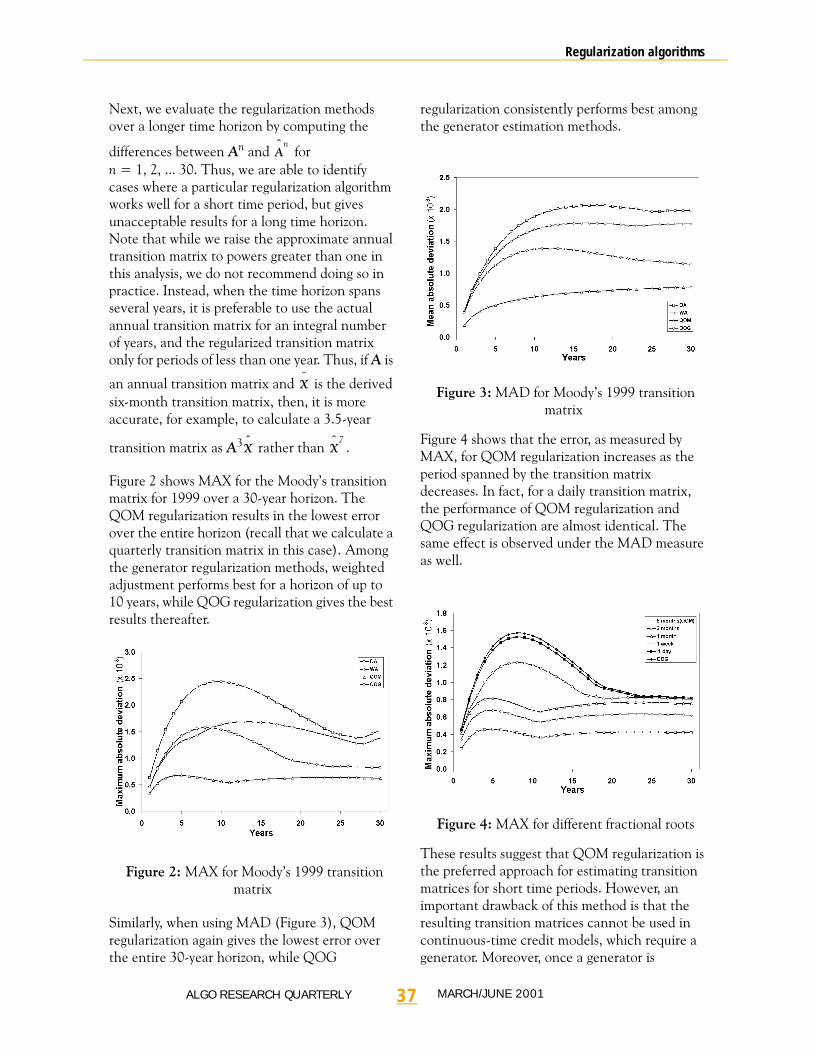
Next, we evaluate the regularization methods over a longer time horizon by computing the

differences between An and for n = 1, 2, ... 30. Thus, we are able to identify cases where a particular regularization algorithm works well for a short time period, but gives unacceptable results for a long time horizon. Note that while we raise the approximate annual transition matrix to powers greater than one in this analysis, we do not recommend doing so in practice. Instead, when the time horizon spans several years, it is preferable to use the actual annual transition matrix for an integral number of years, and the regularized transition matrix only for periods of less than one year. Thus, if A is

an annual transition matrix and is the derived six-month transition matrix, then, it is more accurate, for example, to calculate a 3.5-year

transition matrix as A3 rather than .

Figure 2 shows MAX for the Moody’s transition matrix for 1999 over a 30-year horizon. The QOM regularization results in the lowest error over the entire horizon (recall that we calculate a quarterly transition matrix in this case). Among the generator regularization methods, weighted adjustment performs best for a horizon of up to 10 years, while QOG regularization gives the best results thereafter.

Figure 2: MAX for Moody’s 1999 transition matrix

Similarly, when using MAD (Figure 3), QOM regularization again gives the lowest error over the entire 30-year horizon, while QOG

regularization consistently performs best among the generator estimation methods.

Figure 3: MAD for Moody’s 1999 transition matrix

Figure 4 shows that the error, as measured by MAX, for QOM regularization increases as the period spanned by the transition matrix decreases. In fact, for a daily transition matrix, the performance of QOM regularization and QOG regularization are almost identical. The same effect is observed under the MAD measure as well.

Figure 4: MAX for different fractional roots

These results suggest that QOM regularization is the preferred approach for estimating transition matrices for short time periods. However, an important drawback of this method is that the resulting transition matrices cannot be used in continuous-time credit models, which require a generator. Moreover, once a generator is

Aˆ n

Xˆ

Xˆ

Xˆ 7

37ALGO RESEARCH QUARTERLY MARCH/JUNE 2001

Regularization algorithms

computed, one can easily calculate a transition matrix for any time interval, no matter how small. Thus, the applicability of QOM regularization is limited to discrete-time models.

Finally, we evaluate the impact of the size and the level of migration in the transition matrix on the performance of QOG regularization. Figure 5 plots MAX when QOG regularization is applied to the following matrices:

• 8 × 8, low migration (Moody’s 1999)

• 8 × 8, high migration (KMV 1995)

• 17 × 17, high migration (Algorithmics)

• 18 × 18, low migration (S&P 1999).

The results suggest that the size of the transition matrix does not affect the approximation error. However, the approximation error tends to be larger when transition matrices have a high level of migration.

Figure 5: MAX for QOG regularization

Conclusions

This paper considers the computation of transition matrices for arbitrary time periods based on a given annual transition matrix. Simply calculating roots of the annual transition matrix is not a valid approach because the resulting matrices typically contain negative elements, and, thus, do not represent valid transition matrices. This problem is closely related to the well-known embedding problem for Markov chains. We show that, in most practical cases, the

generator of a particular transitional matrix does not exist and, thus, regularization algorithms are required to find the transition probabilities for time horizons of less than one year.

We demonstrate that the regularization problem can be expressed as a multidimensional, constrained, non-linear optimization problem, whose solution is computationally intensive. We propose an alternative, efficient approach that obtains a valid transition matrix or generator from the root or logarithm, respectively, of the annual transition matrix. Since this transformation is done on a row-by-row basis, the process reduces to solving a set of simple optimization problems.

Evaluating the regularization algorithms on a set of sample problems suggests that approximating the root of the annual transition matrix yields the best results. Given our relatively small number of test cases, we do not draw any formal statistical conclusions in this regard. However, our empirical results do give an indication of the magnitudes of potential approximation errors due to regularization. The results suggest that the use of quasi-optimization is justified by its high precision and computational simplicity. Since the algorithms are very fast, it is feasible to apply all of them, and then select the transition matrix that is most accurate with respect to a chosen error measure.

There are several possible directions for future research. In the transition matrix framework, the most accurate regularization procedure is based on solving problem BAM directly. Thus, solving the corresponding non-linear optimization problem may lead to a better approximation of the transition matrix.

Finally, a large class of credit risk models is based on finite Markov chains with an absorbing state. These models have one significant theoretical disadvantage; namely, the long-term dynamics of the credit states of market participants cannot be described by this type of model because it does not account for the appearance of new companies with a random initial credit state. Therefore, more adequate models can be based on the Markov processes that simulate the birth

38ALGO RESEARCH QUARTERLY MARCH/JUNE 2001

Regularization algorithms

of new market players. In this case, the model estimation starts with the parameters of the generator governing the Markov process, and all the difficulties related to the regularization problem are avoided. This is an interesting problem for future discussions.

Acknowledgements

We are very grateful to Ian Iscoe, Olivier Croissant, Vita Farber, Asif Lakhany, Leonid Merkoulovitch, Rafa Santander and Hans Tuenter for interesting discussions and contributions on the subject. Michael Shtilman of Ambac Financial Group, Inc. made several useful comments on the subject of this paper and informed us that they exploit an algorithm similar to the algorithm of the analytical solution for regularization of the root of the transition matrix in their risk management system.

References

Araten, M. and L. Angbazo, 1997, “Roots of transition matrices: Application to settlement risk,” Chase Manhattan Bank, Practical Paper.

Carette, P., 1995, “Characterizations of embeddable 3 x 3 stochastic matrices with a negative eigenvalue,” New York Journal of Mathematics 1: 120–129.

CreditMetrics: The Benchmark for Understanding Credit Risk, Technical Document, 1997, New York, N.Y.: J.P. Morgan & Co. Inc.

CreditMetricsTM, 2000, (Accessed on the webpage of CreditsMetrics on February 7, 2000)

Das, S. and P. Tufano, 1996, “Pricing credit sensitive debt when interest rates, credit ratings and credit spreads are stochastic,” Journal of Financial Engineering 5(2): 161–198.

Dieci, L., 1996, “Consideration on computing real logarithms of matrices, Hamiltonian logarithms, and skew-symmetric logarithms,” Linear Algebra and Its Applications 244: 35–54.

Frydman, H., 1983, “On a number of Poisson matrices in bang-bang representations for 3 x 3 embeddable matrices,” Journal of Multivariate Analysis 13(3): 464–472.

Global Credit Research, 2000, Moody’s Investor Service, New York, NY.

Israel, R., J. Rosenthal and J. Wei, 2001,“Finding generators for Markov chains via empirical transition matrices, with application to credit raitings,” Mathematical Finance, 11(2): 245-265

Iwanik, A., and R. Shiflett, 1986, “The root problem for stochastic and doubly stochastic operators,” Journal of Mathematical Analysis and Applications 113: 93–112.

Jarrow, R., D. Lando and S. Turnbull, 1997, “A Markov model for the term structure of credit spreads,” Review of Financial Studies 10(2): 481–523.

Karpelevich, F., 1951, “On characteristic roots of matrices with nonnegative elements,” (in Russian) Izvestia Akademii Nauk SSSR, Mathematical Series 15: 361–383.

Kingman, J., 1962, “The imbedding problem for finite Markov chains,” Z. Wahrscheinlichkeitstheorie 1: 14–24.

Lando, D., 1999, “Some elements of rating-based credit risk modeling,” Working Paper, Department of Operations Research, University of Copenhagen, Denmark.

Lando, D., 2000, “Estimating rating transitions: A continuous time approach,” Presentation at the conference on Global Derivantives.

Merkoulovitch, L., 2000, “The projection on the standard simplex,” Algorithmics Inc., Working Paper.

Moler, C. and C. Van Loan, 1978, “Nineteen dubious ways to compute the exponential of a matrix,” SIAM Review, 20(4): 801–836.

Snell, J., 1988, Introduction to Probability, New York, N.Y.: Random House.

Stromquist,W., 1996,“Roots of transition matrices,” Daniel H. Wagner Associates, Practical Paper.

Tuenter, H., 2000, “The minimum -distance

projection onto the canonical simplex: A simple algorithm.” Algorithmics Inc., Working Paper.

L2

39ALGO RESEARCH QUARTERLY MARCH/JUNE 2001

Endnotes

1. It is possible to obtain the set of past historical annual matrices that were published by agencies each year. These data are used extensively by the same sources to construct the averaged annual prediction transition matrices.

40ALGO RESEARCH QUARTERLY MARCH/JUNE 2001