Discontinuity preserving regularization of inverse visual problems

IEEE TRANSACTIONS ON SYSTEMS, MAN, AND CYBERNETICS, VOL. 24, NO. 3, MARCH 1994 455

Discontinuity Preserving Regularization of Inverse Visual Problems

Robert L. Stevenson, Member, ZEEE, Barbara E. Schmitz, and Edward J. Delp, Senior Member, ZEEE

Abstruct- The method of Tikhonov regularization has been widely used to form well-posed inverse problems in low-level vision. The application of this technique usually results in a least squares approximation or a spline fitting of the parameter of interest. This is often adequate for estimating smooth parameter fields. However, when the parameter of interest has discontinuities the estimate formed by this technique will smooth over the discontinuities. Several techniques have been introduced to modify the regularization process to incorporate discontinuities. Many of these approaches however, will themselves be ill-posed or ill-conditioned.

This paper presents a technique for incorporating discontinuities into the reconstruction problem while maintaining a well-posed and well-conditioned problem statement.

The resulting computational problem is a convex functional minimization problem. This method will be compared to previous approaches and examples will be presented for the problems of reconstructing curves and surfaces with discontinuities and for estimating image data. Computational issues arising in both analog and digital implementations will also be discussed.

I. INTRODUCTION N THIS PAPER we address the problem of estimating a I discontinuous parameter field, r from sparse and noisy data

S. We are interested in techniques that are capable of reliably estimating the parameter field given the fact that there are discontinuities in the parameter field, or in one or more of the derivatives of the parameter field. Such estimation problems naturally arise in many low-level computer vision problems [34]. For the problem of visual surface reconstruction, the sparse data is obtained from such low-level vision processes as shape-from-stereo, shape-from-shading, etc. [34]. From this data we wish to estimate the surface depth over a dense mesh of grid points. The surface depth will have depth discontinuities at the edges of objects and will have discontinuities in the first derivative at the comers of objects. In the problem of estimating the optical-flow field of a sequence of images we wish to estimate the two-dimensional vector field of object motion. This vector field will be discontinuous on the boundary of objects moving in front of a static background.

The basis of many classical parameter estimation schemes is the assumption that the parameter field varies smoothly [34]. Therefore, these classical techniques are not appropriate for estimating the piecewise smooth parameter fields that arise in

Manuscript received March 13, 1992; revised April 6, 1993. R. L. Stevenson and B. E. Schmitz are with the Laboratory of Image and

Signal Analysis, Department of Electrical Engineering, University of Notre Dame, Notre Dame, IN 46556.

E. J. Delp is with the Computer Vision and Image Processing Laboratory, School of Electrical Engineering, Purdue University, West Lafayette, IN 47907.

IEEE Log Number 9214600.

low-level vision problems, although they are still often used. In order to form reliable estimates we must incorporate the a priori knowledge that the parameter fields of interest may have discontinuities. The regularizing technique proposed by Tikhonov introduces a priori information into the problem statement through the use of a stabilizing functional. The stabilizing functional measures the consistency of a particular field r* with the a priori assumptions relative to the form of the field. Therefore, one of the important issues to address is an appropriate form for the stabilizing functional.

The Tikhonov regularization technique uses the stabilizing functional to form a functional minimization problem, which is then solved to form the estimated parameter field. If the chosen stabilizing functional is nonconvex, then the resulting computational problem of minimizing a nonconvex functional is itself an ill-posed problem. The nonconvex minimization problem is ill-posed because the solution will no longer vary continuously with a change of the input; i.e., a small change in the input can result in a drastic difference in the output. Because of this ill-posedness the stability of the output may also be affected by the implementation and by quantization noise. Another problem is that although techniques to exist for minimizing such functionals the computational complexity of these algorithms is very high. Thus when considering a possible stabilizing functional it is important to examine the resulting minimization problem in terms of both its stability and computational requirements. For this reason a convex stabilizing functional is highly desirable.

Early approaches to dealing with discontinuities proposed various nonconvex stabilizing functionals and novel methods for dealing with the resulting computational problems [4], [l 11, [121, [261, [271, [30], [31], [39]. Unfortunately, the resulting algorithms are ill-posed and yield unstable results. This paper examines a class of convex stabilizing functionals which yield desirable results when the parameter fields or their derivatives have discontinuities. Section I1 introduces the necessary background from regularization theory that is needed. Section 111 discusses several previous approaches to defining a stabilizing functional which incorporates the a priori knowledge of the existence of discontinuities and characterizes the problems of such algorithms. Section IV introduces a class of convex stabilizing functionals that are useful and characterizes the form of the resulting estimates. Section V discusses some of the computational aspects of minimizing these convex but nonquadratic functionals. Section VI compares the convex regularization kemels with previously proposed nonconvex regularization kernels. It is shown that better reconstructions

0018-9472/94$04.00 0 1994 IEEE

456 EEE TRANSACTIONS ON SYSTEMS, MAN, AND CYBERNETICS, VOL. 24, NO. 3, MARCH 1994

can be obtained with the convex stabilizers in terms of mean absolute and mean squared errors. Computational comparisons and reconstructions using real data are also addressed. Finally Section VII draws some conclusions.

II. REGULARIZATION THEORY

Low-level image analysis problems, because of their inherent structure, are generally inverse problems and like most physical inverse problems the mathematical formulation of the problem statement is ill-posed [l], [33]. The general inverse problem can be stated by the following: find the parameter field r from the observed finite collection of data S = { G } + ~ . For the problem to be well-posed in the sense of Hadamard [14] the solution must exist, be unique, and depend continuously on the data, In image analysis problems the observed data S is generally sparse andor noisy and will not uniquely determine a solution r, hence the problem is ill-posed [34].

To obtain a unique and stable solution from the data, supplementary information must be used so that the problem becomes well-posed [52], [53]. The basic principle common to all methods to use a priori knowledge of the properties of the inverse problem to resolve conflicts in the estimates, and to restrict the space of possible solutions so that the data uniquely determine a stable estimate. Two techniques that are often used to form a well-posed problem for many ill-posed inverse problems are the methods of Tikhonov regularization [52], [53] and stochastic regularization [29], [30].

M

A. likhonov Regularization

To make the problem well-posed, a continuous operator, known as a regularizing operator, is defined which approxi- mates the inverse operator. To construct a regularizing operator, R(. , .), Tikhonov and Arsenin [52] introduce a stabilizing functional, R [ +] . This stabilizing functional provides a measure of the consistency of a particular solution based on the apriori assumptions. The stabilizing functional is used to define the functional

M’[~*,s] = n[r*] + Xil\Ar* - till (1) C , E S

where )I 1 1 is a norm and denotes the process of acquiring the ith data point and is assumed to be linear. This norm measures the distance between a possible solution and the observed data. This term will be large for solutions that are not near the observed data. Let X denote the collection of {&}El. Then, for certain values of A, the minimization of this functional is a regularizing operator,

rx = R ( S , X ) = argminM’[r*,S]. r’

This regularized solution, r’, will be used as the solution estimate which will be denoted as e. Note that the regularizing operator for a particular problem is in general not unique; there may exist many operators which stabilize the ill-posed problem. The choice of the particular operator and the value of the regularization parameter X is based on supplementary information pertaining to the problem.

In summary, to find a regularized solution to an ill-posed problem, a stabilizing functional, Cl[-], must be specified based on a priori information. Then an appropriate X must be found such that the minimization of M’[r*, SI is a regularizing operator. The choice of X will be based on the choice of the stabilizer, the chosen norm, and supplementary information pertaining to noise in the data. Once this information is obtained, the regularized solution, r’, to the ill-posed problem is determined by minimizing the functional M A [r*, SI The hardest task is to find a stabilizer which not only yields a unique and stable solution to the inverse problem, but also accurately measures the consistency of the estimate with respect to the true solution.

If a[-] is chosen so that it is quadratic then it can be shown that the solution space is convex and a unique solution exists [52]. Most applications will therefore define 0[.] to be some norm or semi-norm on the solution space. When this is not the case then the functional may be nonconvex. This makes finding the optimal solution more difficult and ill-posed since there may exist many suboptimal local minimum.

For univariate regularization of scalar functions, Tikhonov proposed a general stabilizer based on the mth-order weighted Sobolev norm. Letflx) be some scalar univariate function, then a general stabilizing functional can be written as

where the wp(x)’s are nonegative and possibly discontinuous weighting functions [52] and m determines the degree of smoothing. Using such a stabilizer makes the problem well- posed by restricting the space of admissible solutions to the Sobolev space of smooth functions. For multivariate vector- valued functions Tikhonov’s suggestion can be generalized for the n-dimensional case to

where p = (p1,p2,..-,pn), I P ( = PI + p z + . * * + p n and x = (XI, 22, . , xn). This multivariate weighted Sobolev norm is the basis on many of the stabilizing norms used in low-level image analysis [34]. Stabilizing functionals of this form measure function smoothness will be lead to algorithms which smooth discontinuities. This functional is also quadratic, thus applications which utilize such stabilizers result in convex optimization problems. In this paper we will examine a more general stabilizing functional with the form

where p( . ) is some scalar function. In this paper we will be examining several possible functions which can be used for p ( - ) . We will show that p ( . ) can be chosen so that the resulting

STEVENSON et al.: DISCONTINUITY PRESERVING REGULARIZATION 451

regularizing functional has the two desirable properties of being convex and allowing discontinuities. Conditions for a stabilizer of the form (5) to be convex are given by the following theorem (the proof is in the Appendix).

Theorem 1: The stabilizer in equation ( 5 ) is convex if and only if the scalar function p ( . ) is convex.

B. Stochastic Regularization

The stochastic solution to ill-posed problems is a straight forward application of Bayesian estimation [ 1 I]. The Tikhonov method makes the problem well-posed by restricting the space of possible solutions to a dense subspace so that a stable and unique solution can be found. The manner in which this restriction is made is based on apriori information. In contrast, a stochastic approach use a priori information relative to the likelihood of a function, r*, being a solution to define a probability distribution, Pr* . A priori information about the observation noise process is used to determine a conditional probability distribution, Using these distributions, the posterior probability distributions can be obtained by

which represents the likelihood of a solution, r*, given that the data, S, was observed. An estimate, r, can then be found with either a MAP estimator or by defining a loss functional and computing a Bayesian estimate. The MAP estimate is found by simply maximizing the probability distribution (6) or the log of the distribution to find the function, e, which is the most likely solution given the data, S, i.e.,

i. = argmax[ln r* PSI.* +In Pr*]. (7)

In summary, to make the problem well-posed, a probabilistic model on the space of possible solutions must be specified based on a priori information. The quality of the solution will depend largely on the quality of the model chosen; thus it is critical that the model accurately reflect the true space of surfaces. The estimated solution is then found by maximizing (or minimizing) a functional. If the measurement process is modeled as having additive Gaussian noise then

where X i = 1/20? and g’ is the variance associated with the ith data point. By choosing a prior with the form

p,. Ex ,-n[r*l (9)

the techniques of Tikhonov and stochastic regularization results in the same functional minimization problem. Using the Sobolev seminorm, (4), for n[.] and by making appropriate discrete approximations, this can be shown to be equivalent to assuming a Markov Random Field (MRF) model for the prior 1471, 1481, where the order of the derivative is equivalent to the order of the MRF. This connection can be used to examine Tikhonov regularization in the context of a probability space P31.

111. MODIFICATIONS TO THE STABILIZING FUNCTIONALS TO INCORPORATE DISCONTINUITIES

In order to incorporate the a priori knowledge that discontinuities exist into the reconstruction process we either examine modifications of the stabilizing function in Tikhonov regularization or the prior distribution function in stochastic regularization. In this section we examine several previously proposed modifications to these functions and the resulting characteristics of the reconstruction algorithms.

A. Controlled-Continuity Stabilizers

If the location and type of discontinuity is known, this information can be easily incorporated into the stabilizing functional through the use of the weight terms, wp(z), in the Sobolev seminorm, (4). For an mth order discontinuity (m = 0 is a jump discontinuity, m = 1 is a discontinuity in the first derivative, etc.) that occurs at the location (x’), set

wp(x’) = 0 , for JpJ 2 m

and for all other locations set the weight term to one. This controls the order of the continuity at discontinuities [49]-[51]. When used in this fashion, the weight term, wp(x), is referred to as a line process since it indicates where lines (Le., edges) exist in the parameter field. The weight term can also be used for other things such as estimating parameter fields which are rotationally invariant 1401, [43], 1441. Since the knowledge of the location and type of discontinuity is rarely known in most applications, the weight term cannot usually be set prior to computing the estimate. Therefore, the weighting function must also be estimated. Approaches based on estimating the weighting function and the reconstructed parameter field separately have been proposed 1131, [181,[251, [261, 1371, 1381, 1391 as well as approaches based on estimating both the weight function and the parameter field together [2]-[5], [51].

The techniques proposed in [13], [18], [25], and [26] make hard decisions about the value of the weight function, Le., wp is set either to 1 or 0. This preprocessing step is essentially performing discontinuity detection on sometimes sparse and noisy data. Since this type of preprocessing requires a decision, these techniques will be prone to unstable reconstructions. This occurs since small perturbations of the data when the decision parameter is near the threshold can result in a different decision being made, and consequently a drastically different parameter field being estimated. A slightly more robust technique was proposed by Sinha and Schunck [37]-[39]. Their method allowed the weighting function to take on any value greater than 0. They perform an initial fit without any discontinuities and then set the weight term to be inversely proportional to the first derivative of the initial estimate. This has the effect of creating a region where the weight term is small near discontinuities and large in regions where the parameter field is smooth. This type of soft decisionmaking will result in a more stable estimate than making a hard decision. The tradeoff is that near discontinuities, where the weight term is small, the noise removal properties of the spline fitting will be defeated. That is, the estimating procedure will produce noisy estimates of the parameter field near the discontinuities. To overcome

458 IEEE TRANSACTIONS ON SYSTEMS, MAN, AND CYBERNETICS, VOL. 24, NO. 3, MARCH 1994

this problem they introduce another parameter which can be used to make the decision harder, i.e., to make the region where the weight term is near zero smaller. Of course, making a harder decision will result in a more unstable estimate.

To form estimates for wp(x) in conjugation with r(x) we cannot simply minimize (1) with respect to wp and r(x) when using the Sobolev seminorm, (4). Doing this would result in the trivial solution wp(x) = 0 and r(x) being only uniquely determined at points where these are constraints.

B. Estimating the Line Process

In order to estimate wp(x) in conjugation with r(x) we need to augment our prior information with some knowledge about the form of wp(x)[51]. This can be done by adding a term to a[.] which measures the consistency of a given wp(x) [51]. That is we minimize a functional of the form

XillAr* -ci112 (10) M’[~*,W~*,S] = fiw[r*,wp*] + c, ES

where a,[., e ] has the form

aW[r*, wp*] = €(r*, wp*) + z)(wP*). (1 1)

The functional E ( . , .) will have a form such as in (4) and I)(.) will measure the consistency of the line process. Unfortunately even for simple D(.) the functional minimization problem becomes nonconvex. This is a problem not only because of the increased computation required for a solution but also because the mathematical problem is no longer well-posed.

Blake and Zisserman proposed a I)(.) which counted the number of discontinuities for a particular wP(x) and used a stabilizer of the norm of (4) for E ( . , e). They showed that this was equivalent to a using standard Tikhonov regularizing functional with a stabilizer of the form of (5) with wp(x) = l , V x and p ( - ) of the form (see Fig. l(a))

This choice for the regularization function will be referred to as the neighborhood interaction function. This choice for p( . ) is nonconvex and thus results in a nonconvex and ill-posed functional minimization problem. Figure l(b) is a plot of the influence functional (the first derivative of p ( - ) ) , it indicates the amount of influence imposed as the derivative term gets larger. For this stabilizer notice that once a threshold is exceeded this term exerts no further influence on the solution.

Similar schemes for estimating he line process were proposed by Geman and Geman [ l l ] and by Marroquin [29], [30]. Their approach also results in a nonconvex and ill-posed functional minimization problems. Several novel techniques have been proposed to overcome some of the computational complexity associated with such an approach [lo], [21]. While the accuracy of signal estimators based on nonconvex optimization may be adequate, the stability of such an approach will be poor. Small noise in the data can dramatically change the result. Even for the same input data and the same functional to minimize, different optimization algorithms can compute very different results. This will be shown in Section VI-B.

2 T T *

IV. CONVEX AND STABLE APPROACHES

As was discussed in the last section, in order for the regularization problem to be well-posed the stabilizing function must be convex. The question then becomes can a convex stabilizing functional be devised such that discontinuities in the parameter field can be accurately reconstructed. In this section we will examine using a stabilizer functional of the form of (5) with some convex p(- ) . The weight terms will be set to some constant value throughout the entire field, that is wp(x) = wp. Since the class of convex functional is very large, we will begin by first discussing other desirable characteristics (besides convexity) which are desirable for the functional p(. ) .

Besides being convex the functional should be symmetric since the sign of a particular term should not change the importance of its magnitude. The most important charac- teristic of course is that discontinuities should be allowed to form. In the previous section the weight term, wp, was used to allow discontinuities, the weight was changed to deemphasize regions where the derivative is large (i.e., regions of discontinuities). Regions of discontinuities can also be deemphasized by modifying p( . ) so that it is less than the squared term, i.e., p(z) < z2 for large values of z. Finally, we would like a parameter, T, which controls the degree of smoothness of the reconstruction, we will denote the parameterization of p( . ) by p T ( - ) . That is, as a parameter T varies from some Tl to T2, the estimated parameter field varies from a smooth reconstruction to a reconstruction that allows more discontinuities. Mathematically this is equivalent to the condition that pT ( ) decreases monotonically as T varies from TI, to T2 for all z. To better understand this condition recall that the stabilizer a[.] measures the consistency of a particular function with our a priori information. If we want a parameter which controls the degree to which discontinuities are allowed (or conversely the degree of smoothness imposed), then for any particular function rl(x) if the parameter T is varied to allow more discontinuities then the consistency measure should decrease. If the pT (.) functional does not decrease monotonically as T is varied then it is easy to devise a function for which the consistency measure will increase as the degree of allowed discontinuities is increased. The desirable properties of p T ( . ) can be summarized

.

by

STEVENSON et al.: DISCONTINUITY PRESERVING REGULARIZATION

1.0

0.8

0.6

0.4

0.2

0.0

459

I .o . ' " ' . ' " . . ~ ' ' ' 1 " ' I . , . , .

0 0 A 0.8'0 0 0 0

0 0 0 0 < ""94"""8"0"".B -0 0 -

0 0 0

0 b -

- - o*o oo 0 - 0 0 0

0 ,g - 0.6 - 0 0 " : - 0 -

0 8 : 0.4 - 0 -

08 0 0 0 0 0

8 O0 8 0

0 00

8 - 0 0

0 0 eo 0 0

8 L O

- 0 0 - o*d%%*%o 0.2 - - 00

0

. . . I . . . I . . , I , . . I . . .

0 20 40 60 80 1w 20 40 60 80 lwo-oo ' ' ' ' . ' . ' '

1) convex, pT[ax + (1 - a)y] 5 apT(z)+ (1 - a ) p T ( y ) .

2) symmetric, pT(x ) = pT(-x), 3) allows regions of discontinuities, p T ( x ) < x2, for 1x1

4) has a parameter which can consistently vary the degree of discontinuities allowed, pT (x) decreases monotonically for all x as a function of T.

To examine some of the characteristics of the functionals that we are going to discuss, we will apply this technique to the problem of approximating piecewise smooth curves from noisy data. The curves will be estimated on a grid on 100 points. There is a discontinuity in the curve near grid point 23, a discontinuity in the first derivative of the curve near grid point 50, and the curve varies smoothly in the region between 55 and 100. Two sets of data will be examined, a set of noisy dense data, Fig. 2(a), and a set of noisy sparse data, Fig. 2(b). The dense data was obtained by sampling at every point and adding Gaussian noise with standard deviation of 0.02. To obtain the sparse data the curve was sampled at every fifth location and Gaussian noise with standard deviation of 0.02 was added to the signal. Let y(x) denote the curve we wish to estimate, then the acquisition process can be modeled by d;g(z) = y(x;). The Stabilizer used in the reconstruction is

x , y E R , a E [O, 11,

large,

x E R,

In this paper we will examine the class of convex stabilizers which can be characterized by the functional (see Fig. 3)

where p , q 2 1, and generally q 5 p. This choice is based on varying the degree of smoothness imposed at different scales. Below some threshold T one weighting function is used while above that threshold a weighting function that increases less rapidly (Le., less smoothness imposed) is used. By choosing

/I

1 T X 1

p > q we smooth small scale noise while retaining large scale discontinuities in the parameter field. The constants in (14) are chosen so that the weight function is convex and continuous and so that the influence function is continuous.

A. A Scale-Invariant Stabilizer

Bouman and Sauer [6], [7] and Harris [21] examine the case where 1.0 5 p 5 2.0 and T = m, which is the special case of (14) when

P ; ( 4 = 1zIP. (15)

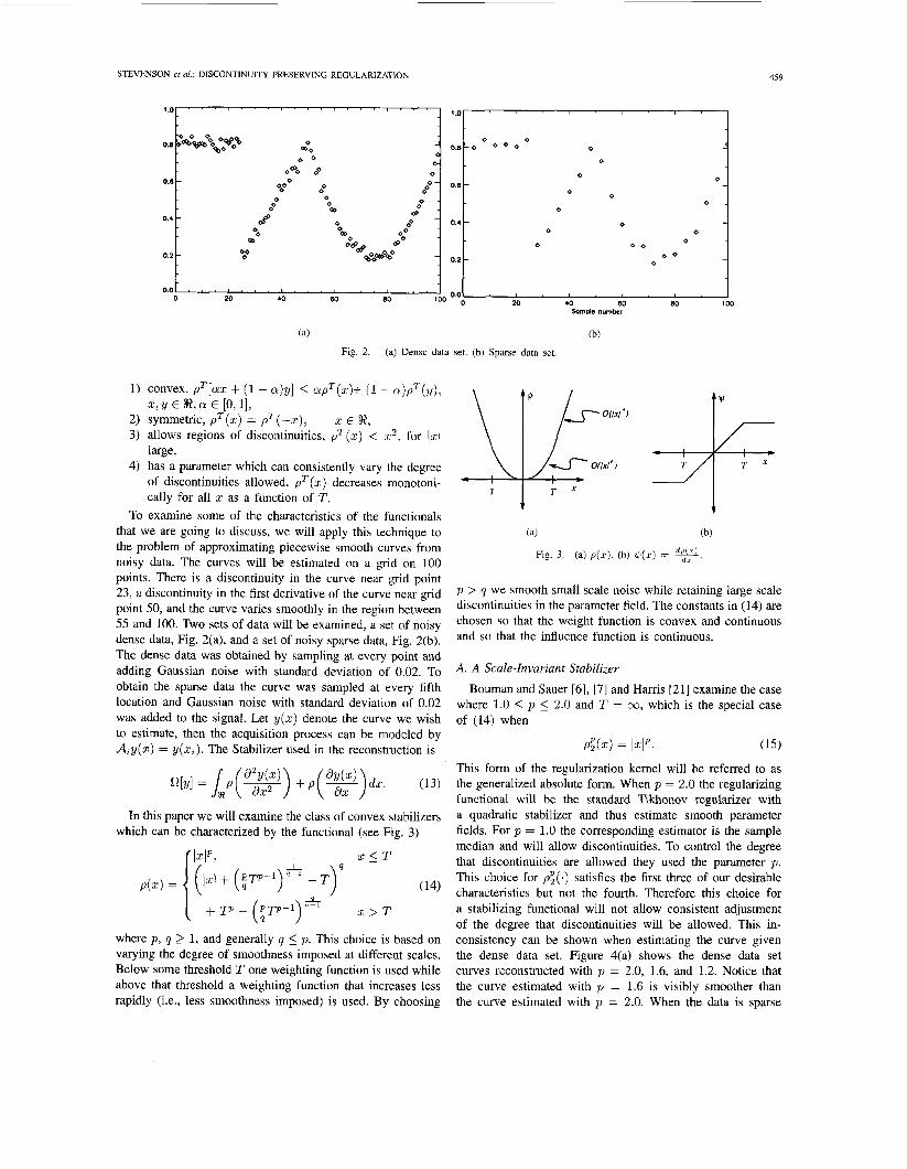
This form of the regularization kernel will be referred to as the generalized absolute form. When p = 2.0 the regularizing functional will be the standard Tikhonov regularizer with a quadratic stabilizer and thus estimate smooth parameter fields. For p = 1.0 the corresponding estimator is the sample median and will allow discontinuities. To control the degree that discontinuities are allowed they used the parameter p . This choice for &(.) satisfies the first three of our desirable characteristics but not the fourth. Therefore this choice for a stabilizing functional will not allow consistent adjustment of the degree that discontinuities will be allowed. This in- consistency can be shown when estimating the curve given the dense data set. Figure 4(a) shows the dense data set curves reconstructed with p = 2.0, 1.6, and 1.2. Notice that the curve estimated with p = 1.6 is visibly smoother than the curve estimated with p = 2.0. When the data is sparse

460 WEE TRANSACTIONS ON SYSTEMS, MAN, AND CYBERNETICS, VOL. 24, NO. 3, MARCH 1994

- p-2.0

...... p-1.8

p-1.2

- - /i 1 'y jj \

0.0 oi 20 40 €4 80 100

(a)

1.0 ' . ' ' . . - ' . - . ' . . . ' ' ' .

0.2 - !

(b)

Fig. 4. (a) Reconstruction for dense data set using p z ( . ) . e) Reconstruction for sparse data set using p2( . ) .

1.0 1 .o ' . ' ' . . . ' . ' ' ' ' . ' ' ' . .

Od

0.6 -

0.4 -

0.2 -

80 100 0.0 0.0 ' . * . . I . . . I . . " ' . '

20 40 €4 80 100 0 20 40

(a) (b)

Fig. 5. (a) Reconstruction for dense data set using p 3 ( . ) . (b) Reconstruction for sparse data set using p3( . )

the estimate formed with this stabilizer also appears to be very sensitive to the selection of the discontinuity parameter. Figure 4(b) shows the curves reconstructed from the sparse data. Notice the drastic difference in the estimate when the discontinuity parameter is adjusted by less than 0.001%. This occurs because it is not possible with the single parameter to provide sufficient smoothness necessary for interpolation while retaining discontinuities in the estimate. In the application in which Bouman and Sauer are interested, the data is dense and they chose the discontinuity parameter to be between 1.0 and 1.2. In this case we computed satisfactory estimates of the curve. Thus, while in general this may not be a good stabilizer, in some applications it may work satisfactorily.

B. Huber Minimax Functional The second special case that we will examine was motivated

by work done by Huber in robust statistics [19], [20]. He was interested in computing smooth estimates when outliers existed in the data set. He proposed to weight the outliers in the data with a functional of the form

where T varies from +oo to 0. This is the special case for when p = 2.0 and q = 1.0. This function varies as a square for values below the threshold and it varies linearly above the threshold. Thus small scale noise is smoothed with a least squares smoother while large scale discontinuities are weighted less by the linear part of the functional. For T = oo we get a smooth estimate and as T approaches zero more discontinuous regions are allewed. This functional has been applied by Stevenson and Delp to the problems of curve [41], [42] and surface [45] reconstruction and by Shulman and Herve [36] for the problem of estimating discontinuous optical flow fields. Using the dense data set the set of curves in Fig. 5(a) were estimated with this stabilizer. The curves reconstructed from the sparse data set are given in Fig. 5(b). Notice that in both cases the curves are estimated with increasing degrees of discontinuity as the parameter T is varied.

C. General Case

There is of course an infinite number of variations on the choice of p and q that can be examined. The correct choice will depend on the particular application and the a priori information that is known. If a good quality reconstruction is available or can be modeled, then p and q can be chosen sta-

STEVENSON et ul.: DISCONTINUITY PRESERVING REGULARIZATION 46 1

tistically by fitting the statistical model in (9) to the available reconstruction. In most cases p should be chosen to be near 2.0 to provide least squares type smoothing of the noise and q chosen to be around 1.0 to reconstruct the discontinuities as sharply as possible with a convex stabilizer. The threshold T will depend on the scale at which discontinuities are present. Since there is a smooth transition in the weight function at the threshold, the quality of the estimate is not very sensitive to the selection of T and the smaller the quantity Ip - q( is the less sensitive the estimate will be to this parameter.

written as a matrix multiplication, that is,

where the matrix Ai,p depends on the location in the mesh and the order of the discontinuity. Most of the terms in A i , p

are zero, the only nonzero terms being given by the difference equation which approximate the derivatives, e.g., (17), (18), and (1 9). Using these approximations the generalized stabilizer function ( 5 ) has the discrete form

nr N

v. COMPUTATIONAL TECHNIQUES Od[rd] = ' ' ' P(WpAi ,prd) . (21) The previous section presented a mathematically well-posed Ipl<mil=l i,=l

technique for estimating parameter fields with discontinuities. The technique results in a convex but nonquadratic fUnC- tional minimization problem. This section examines several computational issues of the resulting mathematical problem statement. The mathematical problem will first be discretized,

Since the acquisition process, ~ ~ ~ ( ~ 1 , the assumed to be linear, the process can be also written as a matrix multiplication, which we will write as .Aird. The resulting discrete regularization functional can be written as

then both digital and analog computational techniques will be N N

examined. m i ( r d , s ) = ... P(WpAi,prd) I p l < m i l = l i , = l

A. Discrete Problem Statement

The finite element method is utilized to discretize the continuous mathematical problem. The function to be estimated, r(x), is discretized on a regular fine-grid mesh. That is r(x) is sampled uniformly along each of its variables. Assume that N samples are taken along each of the variables. This sampling process results in a finite set of nodal variables which will be represented by .(xi) where xi represents the indexed vector quantity ( ~ 1 , ~ ~ ~ ~ 2 . ~ ~ . . . , x , , ,~ ) and each of the indices, z, vary in the range of 1 to N . Using a triangular conforming element for the first order terms gives the discrete approximation to a first order derivative as

-t- X i l l d i r d - Ci1l2 (22) cp ES

where p ( . ) wp, Ai,p, 1 1 . 1 1 , X and A are based on our a priori information about the application and S is the collection of data. To form the discrete parameter field estimate, this functional is minimized with respect to the nodal variables r d .

In the next two subsections, we will examine both digital and analog techniques for minimizing this discrete functional.

B. Digital Descent Methods

The most prevalent class of algorithms for digital convex functional minimization are based on iterative techniques,

dr(xi) - where the update at each iteration monotonically decreases the functional value. Let r$ denote the function value at the i3r" - r ( q 2 , 1 ' ' . 9 TJ,Z,+l% . ' . G,,,,)

" J

(17) lcth iteration. At each iteration the function is updated by - r ( q z l 3 . . . , J j , 1 7 , . . . rn.zn ).

For higher order terms a nonconforming rectangular element can be used. For example for a second order terms the discrete approximation is

and

r$+l = r: + a'pk (23)

where the vector p k is the direction of the update and the scalar ak determines the size of the step taken in the direction. Since our function is convex any of the descent based methods will converge to the optimal solution given any starting vector rz. However overall computational time will depend on the initial guess rz, and the scheme for choosing the update vector p k and step size a'. For a particular application computational time can be dramatically reduced if there exists some quick technique for forming an rough estimate to be used as the initial guess [16], [MI. For example, in the curve reconstruction problem an initial estimate can be formed quickly by fitting a piecewise linear estimate to the data. Similarly, for the surface reconstruction problem a piecewise planar surface can provide an initial guess. Forming this initial estimate is especially helpful when the data is sparse. In applications where the data is sparse and when it is not possible to quickly form an initial estimate, multigrid techniques can be used to improve the computational time [17].


There are many methods for choosing the update vector pk, the conceptually simplest minimization methods choose pk from among the coordinate vectors e l , . . . , e ". This results in univariate relaxation where at each iteration only one component of r$ changes. Another intuitive choice for the update vector is the direction of steepest descent, that is the direction for which the functional will decrease the fastest. The direction of steepest descent is the direction for which

takes on its minimum value as a function of p. If the Z2-norm is used for I I . I I then the direction of steepest descent will be the negative of the gradient vector, i.e.,

pk = -vM,X[~',SS]. (25)

The choices for pk discussed thus far are not guaranteed to converge to a solution in a fixed number of iterations. For linear systems of equations (quadratic optimization problems) the conjugate gradient method has been shown to converge in a bounded number of steps [15]. This minimization method computes a conjugate basis for the linear systems which are used for the update vectors. With this choice for the update vectors, the iterative process can be shown to converge in one cycle through the basis set. For nonquadratic functional optimization problems, conjugate gradient algorithms have been proposed by Daniel [SI and Fletcher and Reeves [9].

Once an update vector is chosen, the next step is to compute the size of the step, ak, which will be taken in that direction. The maximal decrease for a given pk occurs when ak is chosen so as to minimize the functional along that direction,

ak = argminM,X[r; + a p ' , ~ ] . a E R

This results in a univariate nonquadratic minimization problem. In many applications, including the examples presented here, this one-dimensional minimization problem can be approximated by minimization of the osculating parabola.

In this case ak is well-defined and given by

For the applications presented in the previous section, the solutions were computed by first approximating the solution with a piecewise linear approximation, then by using the steepest descent criterion for the update vector and by computing the step size by minimizing the osculating parabola. One of the advantages of these methods is in the inherent parallelism associated with these algorithms. This can be exploited by a mesh of computational nodes which can greatly reduce the total computational times [46].

C. Analog Computational Networks Variational principles, such as the functional minimization

problem arising from regularization theory, have also been solved using analog networks. These networks can be either chemical, electrical or mechanical. This section examines solving the discontinuity preserving regularization functional that has been studied in this paper using analog electrical networks. The class of variational principles which can be solved by an analog electrical network is dictated by Tellegen's Theorem [32]. Basically the properties of convexity and well- posedness will ensure that the resulting network will compute the correct solution. For quadratic variational principles the resulting analog network can be made with linear components, however, for the nonquadratic variational principles presented here the resulting networks will have nonlinear components.

To ease the notational jumble we will only study the construction of a network which will solve the curve reconstruction problem discussed in Section IV. Extensions to other applications should be clear. For curve reconstruction the resulting continuous variational principle is

c ,ES

By taking the derivative of this functional with respect to ~(zi) and setting the equation to zero, the following N nonlinear equations are obtained:

0 = $(Y(Zi+2) - 2Y(Zi+l) + Y ( Z i ) ) - 2.lll(Y(G+l) - 2Y(Zi) + Y ( G - 1 ) ) + $(Y(G) - 2Y(Zi-l) + Y b i - 2 ) )

+ $J(Y(Zi) - Y(Zi-1)) - $J(Y(Xi+l) - Y($i)) + 2Xi(Y(Zi) - ci)2 (31)

where the last term is only present if there exists a constraint on the value of ~ ( x c ; ) . The equations at the boundaries are slightly different. Now examine the network in Fig. 6. The two terminal passive device, c, and the three terminal device, A, can be characterized by their voltage-current relationship as given in Fig. 7. For this network, we can write the following N equations at each node using Kirchhoff s current law:

1 0 = R{$J(Yi+2 - 2Yi+l + Yi) - 2$J(Yi+l - 2% + Yi-1)

2xi -$J(Yi+1 - Yi)} + R ( Y i - C d 2 .

This has the same form as (31), therefore by exciting the network with the constraint controlled voltage sources, the

STEVENSON et aL: DISCONTINUITY PRESERVING REGULAREATION 463

0 0 0

Fig. 6.

- - - 7

I c' I 1: cw I cw

- - - - Network for solving the variational problem.

0

I -R I

0

Fig. 7. Ideal nonlinear circuit elements.

Fig. 8. Circuit elements for a quadratic minimization. node voltages, y1, yz, . . . , Y N , will represent the solution to the variational principle. Theoretically this solution will be obtained instantaneously, however capacitance in any real implementation will cause transients when the constraints are applied. One the network has settled, the solution to the variational principle can be obtained by measuring the node voltages.

The passive elements E and A depend on the form of $(.) that is being implemented. The case of a quadratic functional minimization problem, where $( .) is linear, has been examined [22], [24], [34], [35], and at least one working VLSI chip has been designed and tested [22]. Analog networks have also been proposed for solving some of the nonconvex functionals that arise when incorporating discontinuities information via the methods discussed in Section III [22], [55]. Figure 8 shows the passive devices which can be used to solve the quadratic variational principle. These devices can be modified to be nonlinear through the use of nonlinear devices such as diodes, zener diodes and through the used of active devices such as operational amplifiers [21].

VI. COMPARISONS AND EXAMPLES This section will compare the three main regularization

kernels described in this paper, the neighborhood interaction form, the generalized absolute form, and the Huber minimax form. The non-discontinuity preserving quadratic form will also be included in the comparisons to provide a base for comparison. The Huber minimax, generalized absolute and

quadratic forms are convex and the digital computational techniques described in the previous section are used for computing the signal estimate. For the neighborhood interaction function a continuation method is used to form the estimate [4]. The technique uses a family of p ( . ) varying from a convex form to the final nonconvex form. For each member of the family a steepest descent technique is used to reach a local minimum.

A. Reconstruction Quality

In order to fairly compare the possible reconstruction quality fairly a good set of parameters ( T , p , q , A ) needs to be computed for each regularization kernel. For some of the models some these parameters are specified (e.g., for the Huber based model p = 2, q = 1). Cross-validation [54] is a standard technique and was used to pick the value of A. Cross- validation, however, is not a good technique for picking the discontinuity-preserving parameter, T. It always tends to favor using a value of T which makes the p function quadratic. This is not surprising since it uses an error criterion based on the mean squared error. A more useful heuristic is to select a value of T which will not cause significant overshoot or undershoot at discontinuity boundaries. This was done by selecting a T for which the combination of both overshoot and understood was less than 5% of the discontinuity height. Once T was selected, A was chosen using cross-validation [%I. The values


TABLE I MODEL PARAMETERS USED FOR RECONSTRUCTIONS

Signal Model x T Quadratic 5 .oo - Generalized Absolute 0.20 1.10 Neighborhood Interaction 0.20 1 .00 Huber 0.05 0.05

TABLE II AVERAGE RECONSTRUCTION ERRORS

Signal Model MAE MSE Quadratic 0.006783 0.000264 Generalized Absolute 0.005624 0.000252 Neighborhood Interaction 0.004172 0.000062 Huber 0.003687 O.ooOo26

for T and A for the models of interest are given in Table I. In order to compare reconstruction qualities both the mean

absolute error (MAE) and the mean squared error (MSE) will be computed for each reconstruction. A synthetic data set was created with both smooth regions and regions con- taining discontinuities.Various amounts of noise was added to this known signal and reconstructions were formed using the different reconstruction kernels. The reconstructions were compared with the original data and the MAE and MSE were computed. The MAE and MSE were averaged for over 200 different noise contaminations. The formulas for these error metrics are given by

(33)

The results are shown in Table II. Due to the presence of discontinuities in the signal the

quadratic signal model performs the worse, as expected. The discontinuity-preserving models all do better then the quadratic, with the Huber model performing the best overall. It should be noted that for some of the individual data sets, both the neighborhood interaction function and the generalized absolute did perform better. This indicates that while all of the discontinuity-preserving signal models are capable of computing high quality reconstructions, the Huber based function will on average perform better. This is due primarily to the robustness of the signal estimate with respection to the selection of the model parameters (T,p, q, A) for the Huber model. Small changes in the model parameters for both the neighborhood interaction function and the generalized absolute can cause large changes in the quality of the reconstruction.

B. Stability Issues

Another issue to be considered when choosing a good regularizer is the stability of the estimator. An estimator for which the reconstruction changes dramatically with small changes in the input signal provides unreliable signal estimates. In Section IV-A. the generalized absolute was shown to compute unstable signal estimates in terms of the regularizer parameters. Small

1.5 I 1

1 .o

0.0

I 32 64 96 128

-0.5 I

Fig. 9. Two noisy signal sets with step edge.

32 64 96 -0.5 ‘ Fig. 10. Reconstruction of noisy step edge using neighborhood interaction.

changes in the p parameter can cause large changes in the output estimate in the case of sparse constraints. Note however that small changes in the input constraints will not cause this behavior, that is it stable with respect to the signal noise. This is also true for the entire class of convex stabilizers since small changes in the constraint set does not effect the location of the functional minimum significantly.

For nonconvex stabilizers the output of the estimator can change with small changes in the input signal. This was shown by [28] and can be demonstrated with the following simple example. Consider the noisy signal sets in Fig. 9. One data set is marked with x and the second is marked with 0. Notice that the two data sets are identical except for the 63rd data point which is different by about only 15%. The signal reconstructions for the two data sets using the neighborhood interaction function is shown in Fig. 10. Notice that both the syntactical and statistical properties of the output signal changes significantly. The edge location is no longer clearly defined and the obtained reconstruction is much smoother. Such instability is a very undesirable property of the entire class of nonconvex stabilizers. For any of the convex stabilizers, the difference between the reconstructions for two such similar data sets is very small.

STEVENSON et a/ . : DISCONTINUITY PRESERVING REGULARIZATION

TABLE 111 AVERAGE COMPUTATION TIME (SECONDS)

465

Signal Model Time (sec) ~

Quadratic 20.6 Generallized Absolute 324.9 Neighborhood Interaction 120.7 Huher 23.3

C. Computational Comparison An issue that should not be neglected when comparing

reconstruction techniques is computation time. It is the goal of many image processing systems to operate in real time which puts the limits on the computational complexity of any of the parts of these systems. The time needed to reconstruct a set of constraints using a given signal model varies depending both on the parameters used and the level of sparsity of the data constraints. Table I11 shows the average computation time for the four main types of regularization kernels considered in this paper. The averages where computed for over 600 curve reconstruction examples where the sparsity of the data points varied from 10% to 100%.

The quadratic regularizing function offers the faster per- formance, but of course does not preserve discontinuities. The Huber function cost only slightly more since the main difference from the quadratic function is an extra comparison operation, which can be performed very quickly. The generalized absolute function takes much longer to reach the minimum since the operation of raising a term to a fractional power is a very computationally expensive operation. For the neighborhood interaction function, while the function costs about the same to evaluate as the Huber form, the number of iterations to reach convergence is much longer since it is necessary to minimize each functional in a family of functionals.

Of the discontinuity-preserving regularizing functions the Huber functions does by far the best in terms of computational complexity. This is due to a combination of it being a convex functional and thus generally requiring fewer iterations to reach the minimum and because each evaluation of the Huber function is a computationally fast operation.

D. Example Reconstructions from Real Data

This section details two applications of the discontinuity- preserving regularization kernels proposed in this paper using real data. The first address the problem of three-dimensional surface reconstruction and the second that of image interpolation.

Three-Dimensional Suiface Reconstruction As example application the three-dimensional surface in Fig. 11 was approximated with several stabilizers. Let z ( x , y) denote the surface we wish to approximate and the data acquisition is modeled by A,z(x. y) = z(x, , yz, ). The approximated surfaces were obtained by using the stabilizer

Fig. 1 1 . Original three-dimensional surface data.

Fig. 12. Surface approximated with quadratic stabilizer.

Fig. 13. Surface approximated with discontinuity preserving stabilizer, T = 0.1.

The surface in Fig. 12 was estimated by using X = 1.0 and T = oa, this corresponds to the normal quadratic surface fitting, notice how the discontinuities in the surface are smoothed. In Figs. 13, 14, and 15 the parameter T was set to 0.1, 1.0, and 2.0, respectively. Notice how the degree to which discontinuities are included is controlled by the parameter T. As an example with some real data the sparse three-dimensional data in Fig. 16 was approximated by a dense grid of points. the data was produced by a Technical Arts lOOX scanner (White scanner) at Michigan State University's Pattern Recognition and Image Processing Lab. The approximate surface obtained using A = 1.0 and T = 0.1 is shown in Fig. 17; notice that both jump and orientation discontinuities are accurately estimated.

Image Filtering Various filtering techniques have been de- veloped to suppress the noise in image signals in order to improve the overall quality of the picture. For images, linear filtering operations do not perform well because images


Fig. 14. Surface approximated with discontinuity preserving stabilize T = 1.0.

Fig. 15. Surface approximated with discontinuity preserving stabilizer, T = 2.0.

. ..

x,

Fig. 17. Three-dimensional surface reconstructed with discontii preserving functional.

Fig. 16. Sparse three-dimensional data.

usually contain many sharp edges and thin structures that tend to be smeared or lost in the filtering processing. Non-linear filters based on rank-order operations such as the median and morphological filters do well at preserving edge and image structure, but perform poorly when filtering Gaussian noise out of the image.

Figure 18 shows a segment of a noisy image and the results of filtering with several different nonlinear filters. Figure 18(a) shows the original noisy image data. Figure 18(b) shows the image filtered with an a-trimmed mean (7 x 7 cross window, a = 3). Figure 18(c) shows the image filtered with a median filter (7x7 cross window). Figure 18(d) shows the image

filtered with the proposed regularization technique, with following discontinuity preserving regularization kernel:

iuity

the

: 3 3

Notice that the discontinuity-preserving regularization kernel (Fig. 18(d)) produces the most visually pleasing reconstruction since the discontinuities in the original data are better preserved and the data is well smoothed.

VII. CONCLUSION This paper has presented a mathematically well-posed

method for estimating parameter fields with discontinuities. The proposed method is based on regularization theory where the consistency measure is nonquadratic, but convex. The convexity of the functional is important from both a mathematical and computational viewpoint. It was shown that the class of convex regularizing functions can provide as higher quality (or higher) signal reconstructions without the stability problems or computational problems of the nonconvex forms. The applications of reconstructing piecewise curves/surfaces and of fitting images data were used to demonstrate the usefulness of the proposed method. Finally, some computational issues were discussed and both analog and digital networks were proposed for solving the variational principle.

VnI. APPENDIX: PROOF OF THEOFEM 1 In this appendix we prove the following theorem:

Theorem I: A functional of the form

(E) dX:,P, r(x)) dx

is convex with respect to the function r(x) and fixed wp(x) if and only if the function p ( . ) is convex.

STEVENSON et al.: DISCONTINUITY PRESERVING REGULARIZATION 467

Fig. 18. Image filtering (a) Noisy image. (b) Filtered using a-trimmed mean. (c) Filtered using median. (d) Filtered using discontinuity-preserving regularization kemel.

Proofi Since the differential operators and multiplying by a fixed w,(x) are linear operators, and since a sum of convex functionals is convex, we can examine without loss of generality the convexity of the functional

R[SI = An p(s(x))dx. (37)

A functional is convex if and only if

O[as(x) + (1 - a)t(x)] 5 ~ O [ S ( X ) ] + (1 - a)R[t(x)] (38)

for all possible functions S(X) and t(x) and for all possible

(+) If R[.]is convex then condition (38) is true. If we assume that p(.) is not convex that means that there exists

scalars a E [0, 11. which implies that R is nonconvex since there exists a s(x), t(x) and a such that condition (38) does not hold, this is a contradiction, therefore p( , ) is convex.


(+) If p ( . ) iS Convex then for dl functions S(X) and t(X) [17] W. Hackbusch, Multi-Grid Methods and Applications. Berlin, Ger- many: Springer-Verlag, 1985.

[18] K. Huang, D. Lee, and T. Pavidis, “Edge detection through two- and for all scalars (L: E [O, 11 the inequality

~ dimensional regularization,” in Proc. Workshop on Computer Vision,

[19] P. J. Huber, “Robust Smoothing,” in Robustness in Statistics, R. L. Launer and G. B. Wilkinson, eds. New York John Wiley & Sons, 1981.

[20] P. J. Huber, Robust Statistics. New York: John Wiley & Sons, 1981. [21] J. G. Harris, “Analog models for early vision,” Ph.D. dissertation,

Califomia Institute of Technology, 1991. [221 J. Hutchinson, C. Koch, J. Luo, and C. Mead, “Computing motion using

analog and binary resistive networks,” Computer, pp. 52-62, Mar. 1988. [23] D. Keren and M. Werman, “Variations on Regularization,” in Proc. 10th

Int. Cant on Pattern Recognition, Atlantic City, NJ, June 16-21, 1990,

[24] W. J. Karplus, Analog circuits: Solutions offieldproblem. New York:

[25] D. Lee and T. Pavlidis, “One-dimensional regularization with disconti-

p(as(x) + - a)t(x>) 5 + - a)dt(x)> (41) Mi- Beach, E, Nov. 30-m. 2, 1987, pp. 225-227.

holds. Then

fl[as(x) + (1 - a)t(x)] = + (1 - a)t(x))dx

ap(s(x)) + (1 - a)p(t(x))dx

p ~ . 93-98.

McGraw-Hill, 1958.

Therefore O[.] is convex.

= &[s(x) + (1 - a)R[t(x)]. (42)

0

ACKNOWLEDGMENT The author would like to thank Professors C. Bouman and

K. Sauer for their many useful discussions and Professors P. Flynn and A. Jain for use of their data.

REFERENCES

[ 11 M. Bertero, T. Poggio and V. Torre, “Ill-posed problems in early vision,” Artgcial Intelligence Laboratory Memo, no. 924, Cambridge, MA: MIT, 1986.

[2] A Blake and A. Zissennan, “Invariant surface reconstruction using weak continuity constraints,” in P m . Computer b i o n and Pattern Recognition Cant, Miami, FL, June 22-26, 1986, pp. 62-67.

[3] A. Blake and A. Zisserman, “Some properties of weak continuity constraints and the GNC algorithm,” in P m . Computer vision and Pattern Recognition Con$, Miami, FL, June 22-26, 1986, pp. 656-661.

[4] A. Blake and A. Zisserman, visual Reconstruction, Cambridge, M A MlT Press, 1987.

[5] A. Blake and A Zisserman, “Localizing discontinuities using weak continuity constraints,” Pattem Recog. Lett., vol. 6, pp. 51-59, 1987.

[6] C. Bouman and K. Sauer, “An edge-preserving method for image reconstruction from integral projections,” presented at the Conference on Information Sciences and Systems, The Johns Hopkins University, Baltimore, MD, Mar. 20-22, 1991.

[7] C. Bouman and K. Sauer, “A generalized Gaussian image model for edge-preserving MAP estimation,” IEEE Trans. Image Processing, vol. 2, no. 3, pp. 296-310, July 1993.

[8] J. Daniel, “The conjugate gradient method for linear and nonlinear operator equations,” SIAM J. Numerical Anal., vol. 4, pp. 10-26, 1967.

[9] R. Fletcher and C. Reeves, “Function minimization by conjugate gradients,” Computer J., vol. 7, pp. 149-154, 1964.

[lo] D. Geiger and F. Girosi, “Parallel and deterministic algorithms for MRFs: Surface reconstruction and integration,” IEEE Trans. Pattern Analysis and Machine Intelligence, vol. 13, pp. 401412, 1991.

[ l l ] S. Geman and D. Geman, “Stochastic relaxation, Gibbs distributions and the Bayesian restoration of images,” IEEETruns. Pattem Analysis and Machine Intelligence, vol. PAMI-6, no. 6, pp. 721-741, Nov. 1984.

[12] D. Geman and G. Reynolds, “Constrained restoration and the recovery of discontinuities,” IEEE Trans. Pattern Analysis and Machine Intelligence, vol. 14, no. 3, pp. 367-383, Mar. 1992.

[13] W. E. L. Grimson and T. Pavlidis, “Discontinuity detection for visual surface reconstruction,” Computer Vision, Graphics and I m g e Process- ing, vol. 30, pp. 316-330, 1985.

[I41 J. Hadamard, Lectures on the Cauchy Problem in Linear Partial Differ- ential Equations,

[15] M. R. Hestenes and E. Stiefel, “Methods of conjugate gradients for solving h e a r systems,” J. Res. National Bureau of Standards, vol. 49, no. 6, pp. 409427, Dec. 1952.

[16] J. Jou and A. C. Bovik, “Improved initial approximation and intensity- guided discontinuity detection in visible-surface reconstruction,” Com- puter vision, Graphics and Imuge Processing, vol. 4, no. 3, pp. 292-325, Sept. 1989.

New Haven, CT: Yale University Press, 1923.

nuities,” in P m . First Int. Conj on Computer Vision, London, England, June 8-11, 1987, pp. 572-577.

[26] D. Lee and T. Pavlidis, “One-dimensional regularization with discontinuities,” IEEE Trans. Pattern Analysis and Machine Intelligence, vol. 10, no. 6, pp. 822-829, Nov. 1988.

[27] S. 2. Li, “Reconstruction without discontinuities,” in Proc. Third Int. Cor$ on Computer vision, Osaka, Japan, Dec. 4-7, 1990, pp. 709-712.

[28] A. Lumsdaine, J. L. Wyatt, Jr., and I. M. Elfadel, “Nonlinear analog networks for image smoothing and segmentation,” J. VLSI Signal Processing, no. 2, pp. 53-68, 1991.

[29] J. L. Marrquin, “Probabilistic Solution of Inverse Problems,” Ph.D. dissertation, Department of Electrical Engineering and Computer Science, Massachusetts Institute of Technology, 1985.

[30] J. L. Marrquin, S. Mitter, and T. Poggio, “Probabilistic solution of ill- posed problems in computational vision,” J. Amer. Statist. Assoc., vol. 82, no. 397, pp. 7689, Mar. 1987.

[31] D. Mumford and 3. Shah, “Optimal approximations of piecewise smooth functions and associated variational problems,” Communications in Pure and Applied Mathematics, vol. 42, pp. 577-685, 1989.

[32] P. Penfield, R. Spence, and S . Duinker, Telkgen’s Theorem and Elec- trical Networks. Cambridge, M A MlT Press, 1970.

[33] T. Poggio and V. Torre, “Ill-posed problems and regularization analysis in early vision,” Artificial Intelligence Laboratory Memo, no. 773, Cambridge, MA. MIT, 1984.

[34] T. Poggio, V. Torre, and C. Kock, “Computational vision and regulm- ization theory,” Nature, vol. 317, no. 26, pp. 314-319, Sept. 1985.

[35] T. Poggio, “Early vision: From computational structure to algorithms and parallel hardware,” in Human and Machine Vision 11, A. Rosenfeld, ed. Academic Press, 1986, pp. 190-206.

[36] D. Shulman and J. Y. Hervd, “Regularization of discontinuous flow fields,” in P m . IEEE Workshop on Visual Motion, M e , CA, Mar.

[37] S. S. Sinha and B. G. Schunck, “Discontinuity preserving surface reconstruction,” in Proc. IEEE Con$ on Computer Vision and Pattern Recognition, San Diego, CA, June 4-8, 1989, pp. 229-234.

[38] S. S. Sinha and B. G. Schunck, “A robust method for surface reconstruction,” in Proc. Int. Workshop on Robust Computer Vision, Seattle,

[39] S. S. Sinha and B. G. Schunck, “Surface approximation using weighted splines,” presented at the IEEE Conference on Computer Vision and Pattern Recognition, Lahaina, Maui, Hawaii, June 3-6, 1991.

[40] R. L. Stevenson and E. J. Delp, “Invariant recovery of surfaces in m- dimensional space from sparse data,” J. Opt. SOC. Amer. A, vol. 7, no. 3, pp. 480-490, Mar. 1990.

[41] R. L. Stevenson, “Invariant reconstruction of curves and surfaces with applications in computer vision,” Ph.D. dissertation, Purdue University, 1990.

[42] R. L. Stevenson and E. J. Delp, “Fitting curves with discontinuities,” in IEEE Int. Workshop on Robust Computer Vision, Seattle, WA, Oct 1-3,

[43] R. L. Stevenson and E. J. Delp, “Viewpoint invariant recovery of visual surfaces from sparse data,’’ in Proc. IEEE Third Int. Con& on Computer Vision, Osaka, Japan, Dec. 4-7, 1990, pp. 309-312.

[44] R. L. Stevenson and E. J. Delp, “Viewpoint invariant recovery of visual surfaces from sparse data,” IEEE Trans. Pattern Analysis and Machine Intelligence, vol. 14, no. 9, pp. 897-909, Sept. 1992.

[45] R. L. Stevenson and E. J. Delp, “Surface reconstruction with discontinuities,” presented at the SPIE Conference on Computer Vision and Graphics II, Boston, MA, Nov. 1991.

20-22, 1989, pp. 81-86.

WA, Oct. 1-3, 1990, pp. 183-199.

1990, pp. 127-136.

STEVENSON et ai.: DISCONTINUITY PRESERVING REGULARIZATION 469

[46] R. L. Stevenson, G. B. Adams, L. H. Jamieson and E. J. Delp, “Parallel implementation for iterative image restorahon algonthms on a parallel DSP machine,” J. VLSI Signal Processing, vol. 5, no. 3 3 , pp. 261-272, 1993. both in electrical engineering.

[47] R Szeliski, “Regularization uses fractal pnors,” in Sixth Nat. Con$ on Art$cial Intelligence, Seattle, WA, July 13-17, 1987, pp. 749-754.

[48] R. Szeliski, Bayesian Modeling of Uncertamty in Low-Level Vision. Boston, MA: Kluwer Academc, 1989.

[49] D. Terzopoulos, “The role of constraints and discontmuities in visible- surface reconstruction,” in Proc. 8th Int. Joint Con$ on Artikial Intel- ligence, Karlsruhe, West Germany, Aug. 8-12, 1983, pp. 1073-1077.

[50] D. Terzopoulos, “Controlled-smoothness stabilizers for the regulariza-

Image Understanding Workshop, New Orleans, LA, Oct. 3 4 , 1984, pp.

[5 1 I D. Terzopoulos, “Regulanzation of inverse visual problems involving discontinuities,” IEEE Trans. Pattem Analysis and Machine Intelligence, vol. PAMI-8, no. 4, pp. 413424, July 1986.

[52] A. N. Tikhonov and V. Y. Arsenin, Solutions of Ill-Posed Problems. Washington, DC: V. H. Winston & Sons, 1977.

[53] A. N. Tikhonov and A. V. Goncharsky, eds., Ill-Posed Problems in the

Barbara E. Schmitz received the B.S degree in 1989 from Marquette University and the M.S. degree in 1993 from the University of Notre Dame,

From 1986 to the present she has been periodi- cally employed with the Naval Research Laboratory in Washington, DC, working on mihtary identifi- cation systems. She is currently working toward the Ph.D. degree in electrical engmeering at the University of Notre Dame under a fellowship from the Clare Boothe Luce Foundation. Her research

tion of Ill-posed problems lnvo~vlng discontinuities," in proc. interests are in the Of vision and image processing‘ Ms. Schmitz is a member of Tau Beta Pi and Eta Kappa Nu.

225-229.

Natural Sciences. Moscow: MIR Publishers, 1987. 1541 G. Wahba, “Spline base, regularization, and generalized cross validation

for solving approximation problems with large quantities of noisy data,” in Approximarion Theory Ill: Proc.eedings of a Conference Honoring Professor George G. Lorentz, E. W. Cheney, ed., Academic Press, pp.

[55] A. L. Yuille, “Energy functions for early vision and analog networks,” Biol. Cybem., vol. 16, pp. 115--123, 1989.

[56] B. E. Schmitz and R. L. Stevenson, “Parameter estimation for the curve recovery schedule,”in Proc. 31st Ann. Allerton ConJ on Communica- tions, Control, and Computing, Monticello, IL, 1993, pp. 485494.

905-912, 1980.

Robert L. Stevenson (S’84-M’90) received the B E.E. degree (summa cum laude) from the Uni- versity of Delaware In 1986 and the Ph.D. degree in electncal engineenng from Purdue University in 1990.

He joined the faculty of the Department of Elec- trical Engineering at the university of Notre Dame in 1990, where he is currently an Assistant Profes- sor. While at Purdue, he was supported by graduate fellowships from the National Science Foundation, the duPont Corporation, and Phi Kappa Phi. His

research interests include multidimensional signal processing, electronic imaging, and computer vision.

Dr Stevenson is a member of Phi Kappa Phi, Tau Beta Pi, and Eta Kappa Nu.

Edward J. Delp (SM’86) received the B.S.E.E. (cum laude) and M.S. degrees from the University of Cincinnati, OH, and the Ph.D. degree from Purdue University, West Lafayette, IN.

From 1980-1984, he was with the Department of Electrical and Computer Engineering at the Univer- sity of Michigan. Since 1984, he has been with the School of Electrical Engineering at Purdue Univer- sity, where he is a Professor of Electrical Engineer- ing. His research interests include ill-posed inverse problems in computational vision, nonlinear filtering

using mathematical morphology, image coding, and medical imaging. He has also consulted for various companies and government agencies in the areas of signal and image processing, robot vision, pattem recognition, and secure communications.

Dr. Delp is a member of Tau Beta Pi, Eta Kappa Nu, Phi Kappa Phi, Sigma Xi, the Optical Society of America, the Pattem Recognition Society, and SPIE. He is an Associate Editor of IEEE Transactions on Pattern Analysis and Machine Intelligence. He is also co-editor of the book Digital Cardiac Imaging. In 1990 he received the Honeywell Award and in 1992 the D. D. Ewing Award, both for excellence in teaching. In 1990 he received a Fulbnght Fellowship to teach and perform research at the Universitat Politecnica de Catalunya in Barcelona, Spain.

Discontinuity preserving regularization of inverse visual problems

Documents

Transcript of Discontinuity preserving regularization of inverse visual problems