Search Algorithms
190
Search Algorithms 3 AI Slides (7e) c Lin Zuoquan@PKU 1998-2021 3 1
-
Upload
khangminh22 -
Category
Documents
-
view
2 -
download
0
Transcript of Search Algorithms

Search Algorithms
3
AI Slides (7e) c© Lin Zuoquan@PKU 1998-2021 3 1
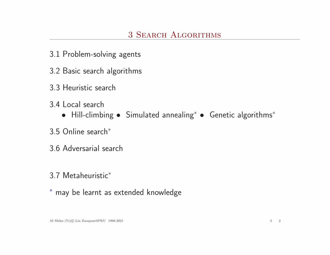
3 Search Algorithms
3.1 Problem-solving agents
3.2 Basic search algorithms
3.3 Heuristic search
3.4 Local search• Hill-climbing • Simulated annealing∗ • Genetic algorithms∗
3.5 Online search∗
3.6 Adversarial search
3.7 Metaheuristic∗
∗ may be learnt as extended knowledge
AI Slides (7e) c© Lin Zuoquan@PKU 1998-2021 3 2
Problem-solving agents
Problem-solving agents: finding sequences of actions that lead todesirable states (goal-based)
State: some description of the current world states– abstracted for problem solving as state space
Goal: a set of world states
Action: transition between world states
Search: the algorithm takes a problem as input and returns a solutionin the form of an action sequence
The agent can execute the actions in the solution
AI Slides (7e) c© Lin Zuoquan@PKU 1998-2021 3 3
Problem-solving agents
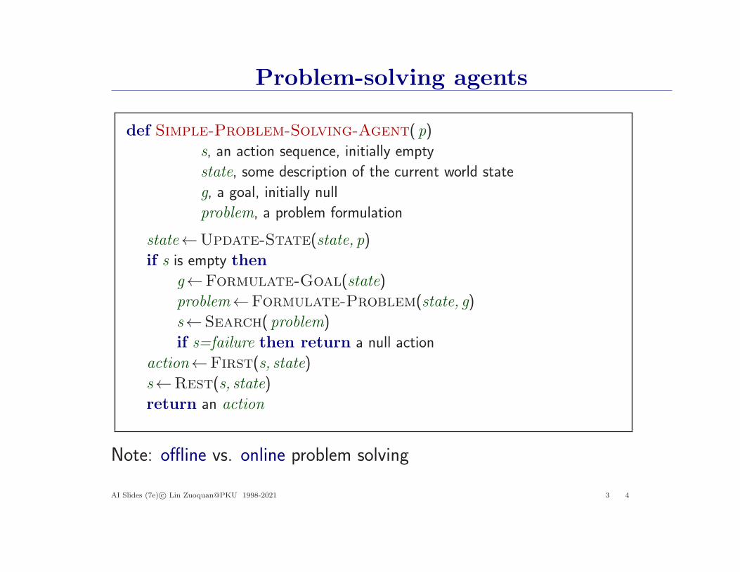
def Simple-Problem-Solving-Agent( p)
s, an action sequence, initially empty
state, some description of the current world state
g, a goal, initially null
problem, a problem formulation
state←Update-State(state, p)
if s is empty then
g←Formulate-Goal(state)
problem←Formulate-Problem(state, g)
s←Search( problem)
if s=failure then return a null action
action←First(s, state)
s←Rest(s, state)
return an action
Note: offline vs. online problem solving
AI Slides (7e) c© Lin Zuoquan@PKU 1998-2021 3 4
Example: Romania
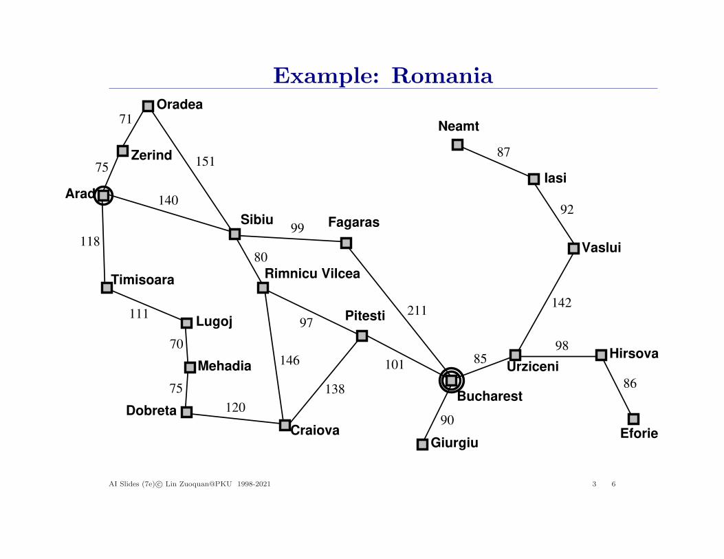
On holiday in Romania, currently in AradFlight leaves tomorrow from Bucharest
Formulate goal:be in Bucharest
Formulate problem:states: various citiesactions: drive between cities
Find solution:sequence of cities, e.g., Arad, Sibiu, Fagaras, Bucharest
AI Slides (7e) c© Lin Zuoquan@PKU 1998-2021 3 5
Example: Romania
Giurgiu
UrziceniHirsova
Eforie
Neamt
Oradea
Zerind
Arad
Timisoara
Lugoj
Mehadia
Dobreta
Craiova
Sibiu Fagaras
Pitesti
Vaslui
Iasi
Rimnicu Vilcea
Bucharest
71
75
118
111
70
75
120
151
140
99
80
97
101
211
138
146 85
90
98
142
92
87
86
AI Slides (7e) c© Lin Zuoquan@PKU 1998-2021 3 6
Problem types
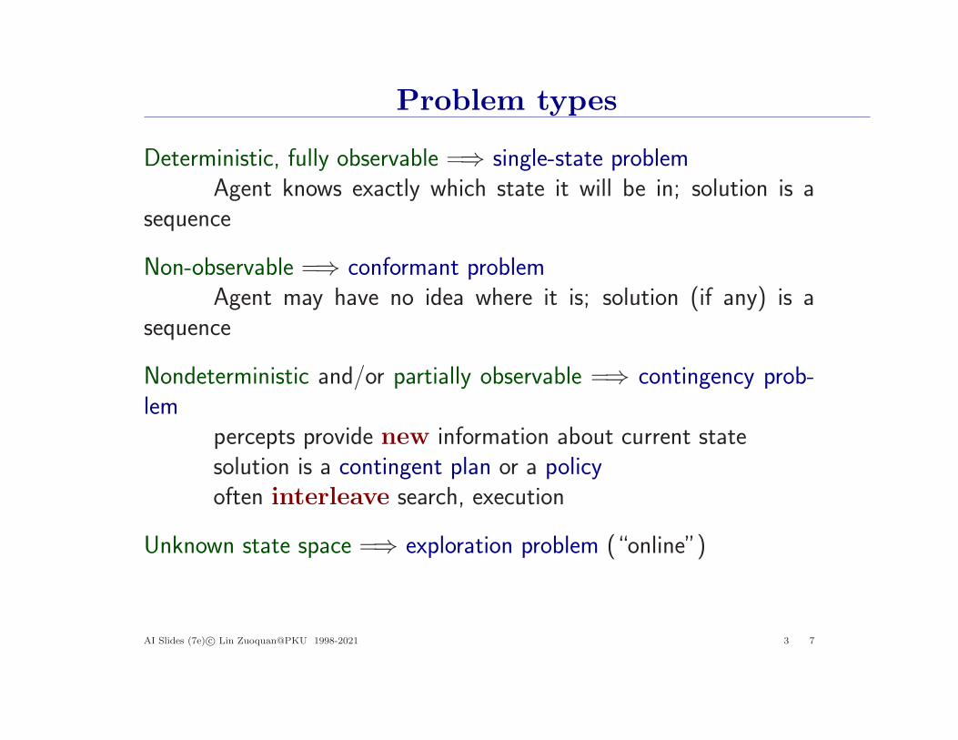
Deterministic, fully observable =⇒ single-state problemAgent knows exactly which state it will be in; solution is a
sequence
Non-observable =⇒ conformant problemAgent may have no idea where it is; solution (if any) is a
sequence
Nondeterministic and/or partially observable =⇒ contingency prob-lem
percepts provide new information about current statesolution is a contingent plan or a policyoften interleave search, execution
Unknown state space =⇒ exploration problem (“online”)
AI Slides (7e) c© Lin Zuoquan@PKU 1998-2021 3 7
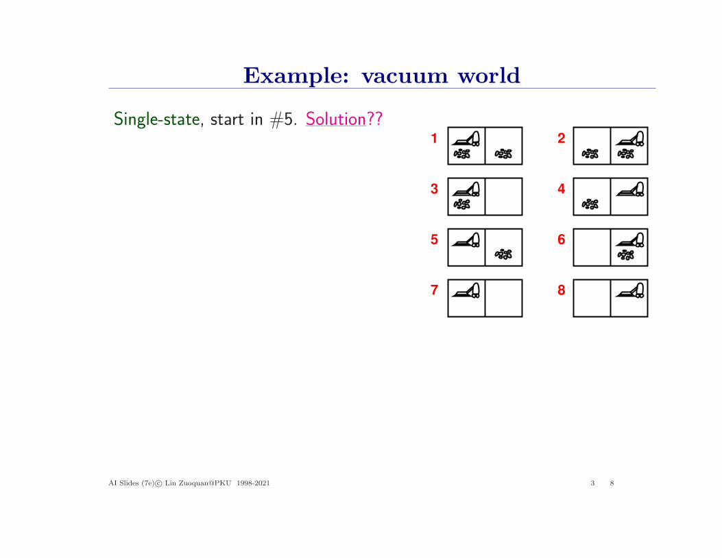
Example: vacuum world
Single-state, start in #5. Solution??1 2
3 4
5 6
7 8
AI Slides (7e) c© Lin Zuoquan@PKU 1998-2021 3 8

Example: vacuum world
Single-state, start in #5. Solution??[Right, Suck]
Conformant, start in {1, 2, 3, 4, 5, 6, 7, 8}e.g., Right goes to {2, 4, 6, 8}.Solution??
1 2
3 4
5 6
7 8
AI Slides (7e) c© Lin Zuoquan@PKU 1998-2021 3 9

Example: vacuum world
Single-state, start in #5. Solution??[Right, Suck]
Conformant, start in {1, 2, 3, 4, 5, 6, 7, 8}e.g., Right goes to {2, 4, 6, 8}.Solution??[Right, Suck, Left, Suck]
Contingency, start in #5Murphy’s Law: Suck can dirty a cleancarpetLocal sensing: dirt, location onlySolution??
1 2
3 4
5 6
7 8
AI Slides (7e) c© Lin Zuoquan@PKU 1998-2021 3 10
Example: vacuum world
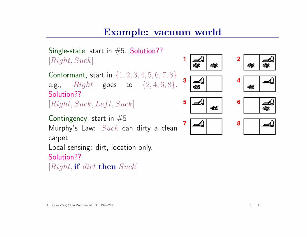
Single-state, start in #5. Solution??[Right, Suck]
Conformant, start in {1, 2, 3, 4, 5, 6, 7, 8}e.g., Right goes to {2, 4, 6, 8}.Solution??[Right, Suck, Left, Suck]
Contingency, start in #5Murphy’s Law: Suck can dirty a cleancarpetLocal sensing: dirt, location only.Solution??[Right, if dirt then Suck]
1 2
3 4
5 6
7 8
AI Slides (7e) c© Lin Zuoquan@PKU 1998-2021 3 11
Problem formulation
A problem is defined formally by five components
initial state that the agent starts– any state s ∈ S (set of states), the initial state S0 ∈ Se.g., In(Arad) (“at Arad”)
actions: given a state s, Action(s) returns the set of actions thatcan be executed in s
e.g., from the state In(Arad), the applicable actions are{Go(Sibiu), Go(T imisoara), Go(Zerind)}
transition model: a function Result(s , a) (or Do(a, s)) that re-turns the state that results from doing action a in the state s;
– also use the term successor to refer to any state reachable froma given state by a single action
e.g.,Result(In(Arad), Go(Zerind)) = In(Zerind)
AI Slides (7e) c© Lin Zuoquan@PKU 1998-2021 3 12
Problem formulation
goal test, can beexplicit, e.g., x = In(Bucharest)implicit, e.g., NoDirt(x)
cost (action or path): function that assigns a numeric cost to eachpath (of actions)
e.g., sum of distances, number of actions executed, etc.c(s, a, s′) is the step cost, assumed to be ≥ 0
A solution is a sequence of actions– [a1, a2, · · · , an]
leading from the initial state to a goal state
AI Slides (7e) c© Lin Zuoquan@PKU 1998-2021 3 13
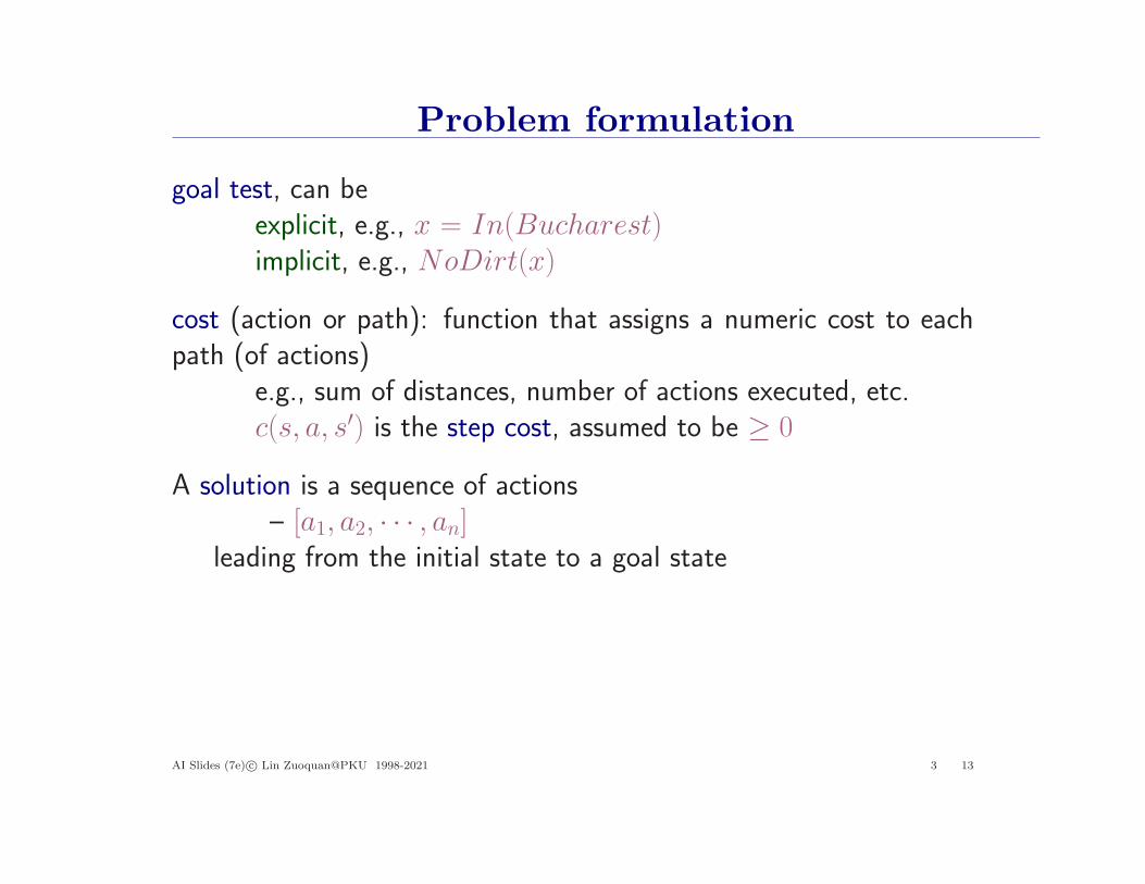
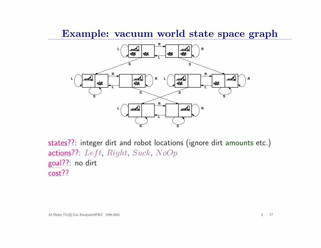
Example: vacuum world state space graphR
L
S S
S S
R
L
R
L
R
L
S
SS
S
L
L
LL R
R
R
R
states??actions??goal??cost??
AI Slides (7e) c© Lin Zuoquan@PKU 1998-2021 3 14
Example: vacuum world state space graphR
L
S S
S S
R
L
R
L
R
L
S
SS
S
L
L
LL R
R
R
R
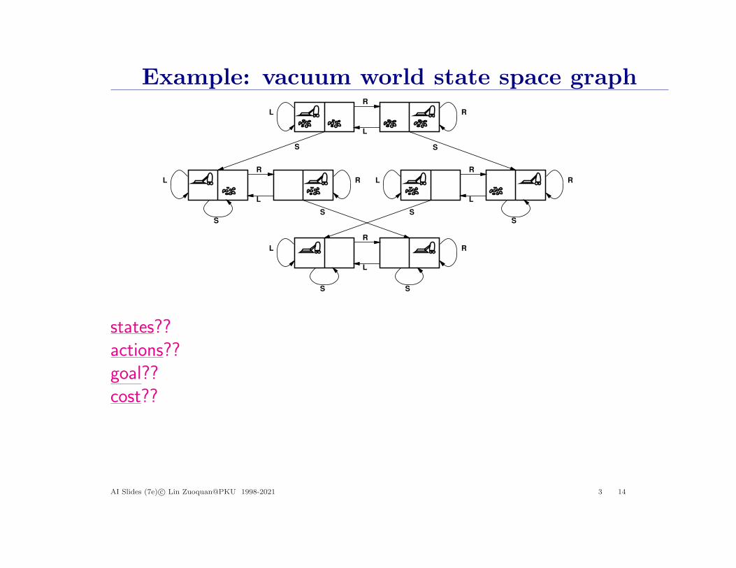
states??: integer dirt and robot locations (ignore dirt amounts etc.)actions??goal??cost??
AI Slides (7e) c© Lin Zuoquan@PKU 1998-2021 3 15
Example: vacuum world state space graphR
L
S S
S S
R
L
R
L
R
L
S
SS
S
L
L
LL R
R
R
R
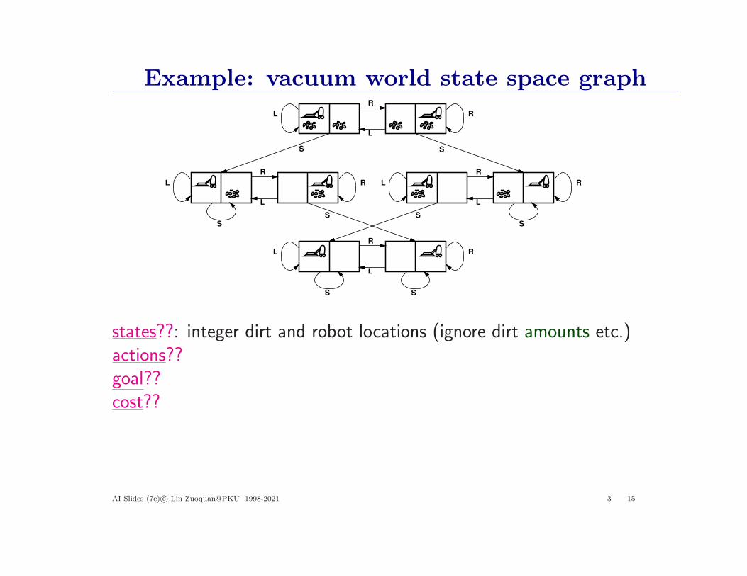
states??: integer dirt and robot locations (ignore dirt amounts etc.)actions??: Left, Right, Suck, NoOpgoal??cost??
AI Slides (7e) c© Lin Zuoquan@PKU 1998-2021 3 16
Example: vacuum world state space graphR
L
S S
S S
R
L
R
L
R
L
S
SS
S
L
L
LL R
R
R
R
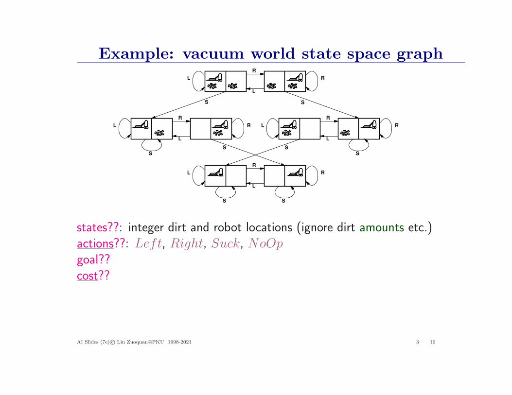
states??: integer dirt and robot locations (ignore dirt amounts etc.)actions??: Left, Right, Suck, NoOpgoal??: no dirtcost??
AI Slides (7e) c© Lin Zuoquan@PKU 1998-2021 3 17

Example: vacuum world state space graphR
L
S S
S S
R
L
R
L
R
L
S
SS
S
L
L
LL R
R
R
R
states??: integer dirt and robot locations (ignore dirt amounts etc.)actions??: Left, Right, Suck, NoOpgoal??: no dirtcost??: 1 per action (0 for NoOp)
AI Slides (7e) c© Lin Zuoquan@PKU 1998-2021 3 18
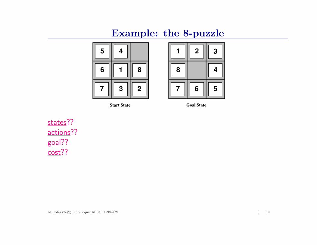
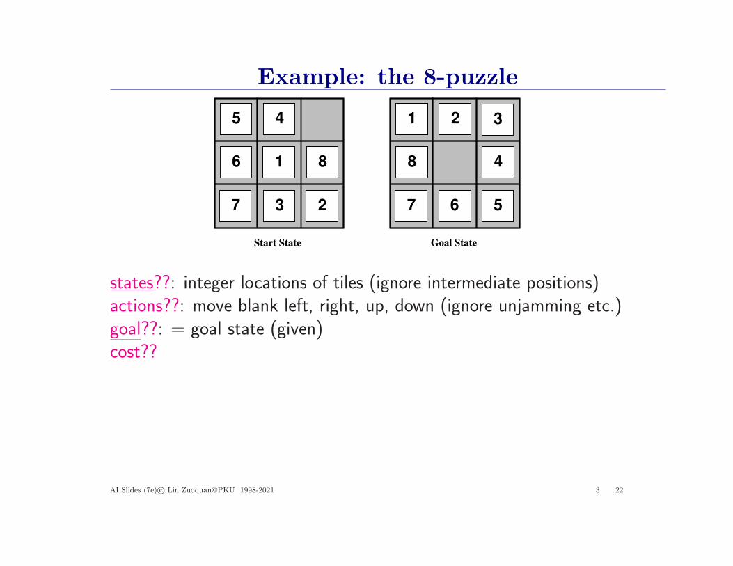
Example: the 8-puzzle
Start State Goal State
2
45
6
7
8
1 2 3
4
67
81
23
45
6
7
81
23
45
6
7
8
5
states??actions??goal??cost??
AI Slides (7e) c© Lin Zuoquan@PKU 1998-2021 3 19
Example: the 8-puzzle
Start State Goal State
2
45
6
7
8
1 2 3
4
67
81
23
45
6
7
81
23
45
6
7
8
5
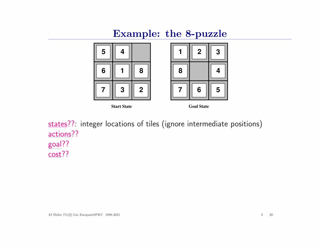
states??: integer locations of tiles (ignore intermediate positions)actions??goal??cost??
AI Slides (7e) c© Lin Zuoquan@PKU 1998-2021 3 20
Example: the 8-puzzle
Start State Goal State
2
45
6
7
8
1 2 3
4
67
81
23
45
6
7
81
23
45
6
7
8
5
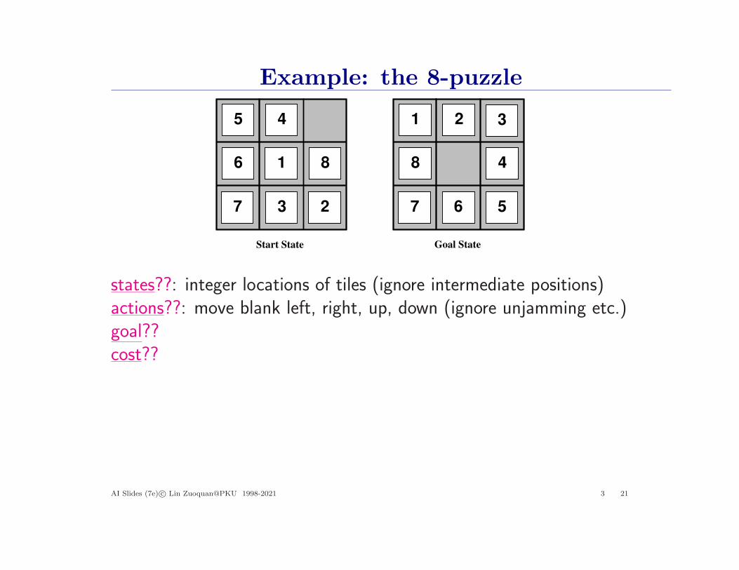
states??: integer locations of tiles (ignore intermediate positions)actions??: move blank left, right, up, down (ignore unjamming etc.)goal??cost??
AI Slides (7e) c© Lin Zuoquan@PKU 1998-2021 3 21
Example: the 8-puzzle
Start State Goal State
2
45
6
7
8
1 2 3
4
67
81
23
45
6
7
81
23
45
6
7
8
5
states??: integer locations of tiles (ignore intermediate positions)actions??: move blank left, right, up, down (ignore unjamming etc.)goal??: = goal state (given)cost??
AI Slides (7e) c© Lin Zuoquan@PKU 1998-2021 3 22
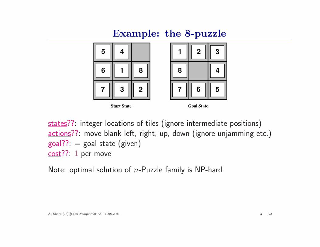
Example: the 8-puzzle
Start State Goal State
2
45
6
7
8
1 2 3
4
67
81
23
45
6
7
81
23
45
6
7
8
5
states??: integer locations of tiles (ignore intermediate positions)actions??: move blank left, right, up, down (ignore unjamming etc.)goal??: = goal state (given)cost??: 1 per move
Note: optimal solution of n-Puzzle family is NP-hard
AI Slides (7e) c© Lin Zuoquan@PKU 1998-2021 3 23
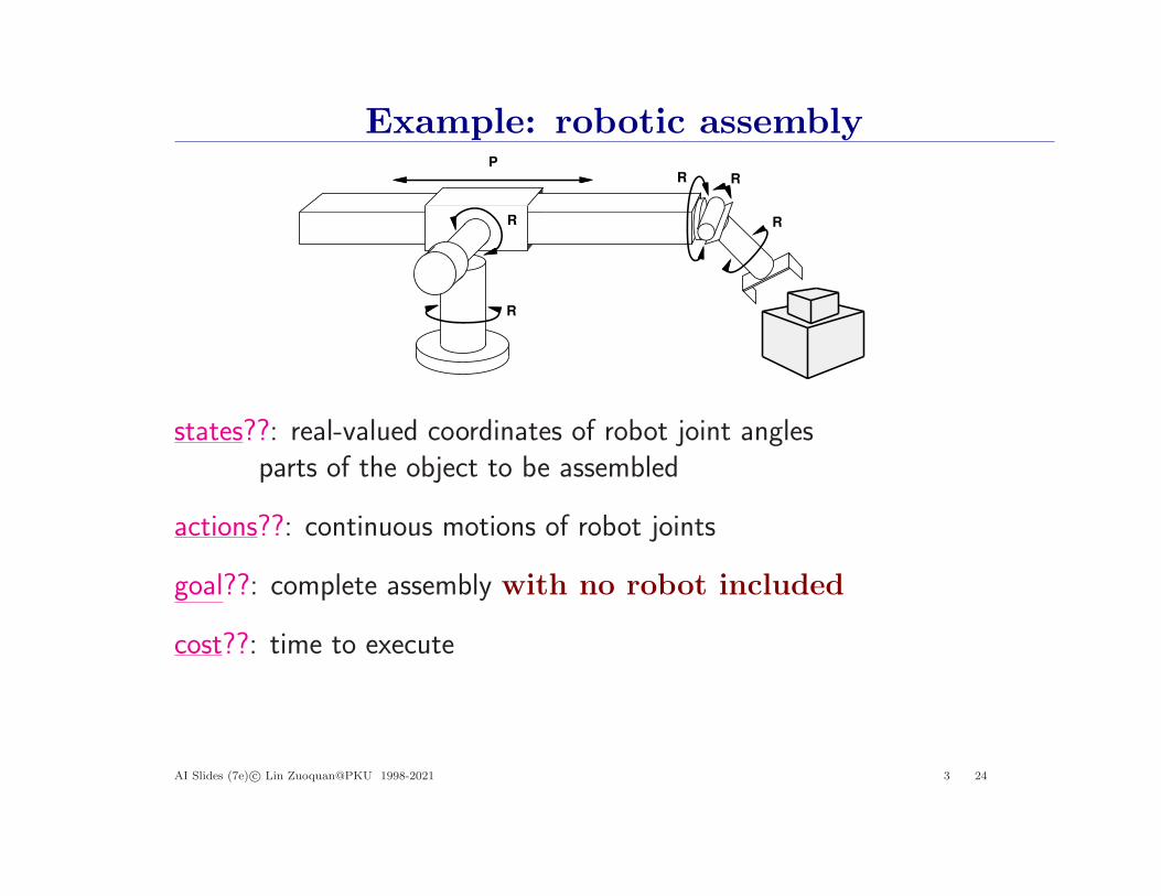
Example: robotic assembly
R
RRP
R R
states??: real-valued coordinates of robot joint anglesparts of the object to be assembled
actions??: continuous motions of robot joints
goal??: complete assembly with no robot included
cost??: time to execute
AI Slides (7e) c© Lin Zuoquan@PKU 1998-2021 3 24
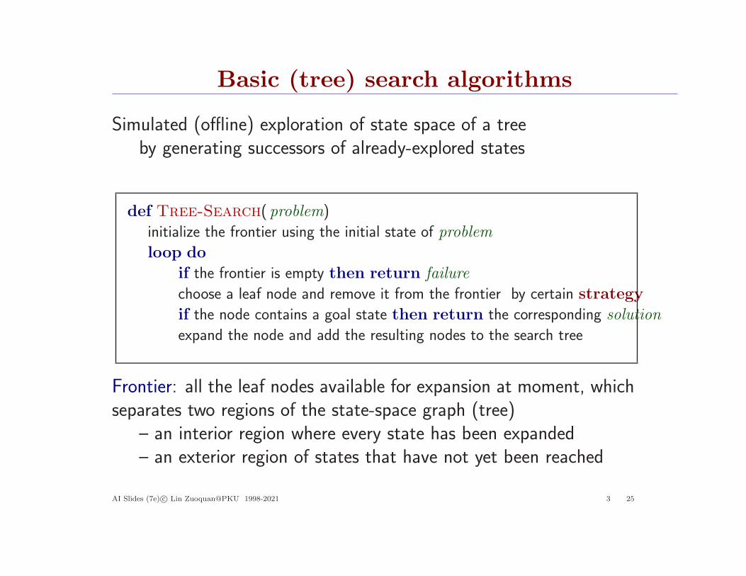
Basic (tree) search algorithms
Simulated (offline) exploration of state space of a treeby generating successors of already-explored states
def Tree-Search( problem)
initialize the frontier using the initial state of problem
loop do
if the frontier is empty then return failure
choose a leaf node and remove it from the frontier by certain strategy
if the node contains a goal state then return the corresponding solution
expand the node and add the resulting nodes to the search tree
Frontier: all the leaf nodes available for expansion at moment, whichseparates two regions of the state-space graph (tree)
– an interior region where every state has been expanded– an exterior region of states that have not yet been reached
AI Slides (7e) c© Lin Zuoquan@PKU 1998-2021 3 25
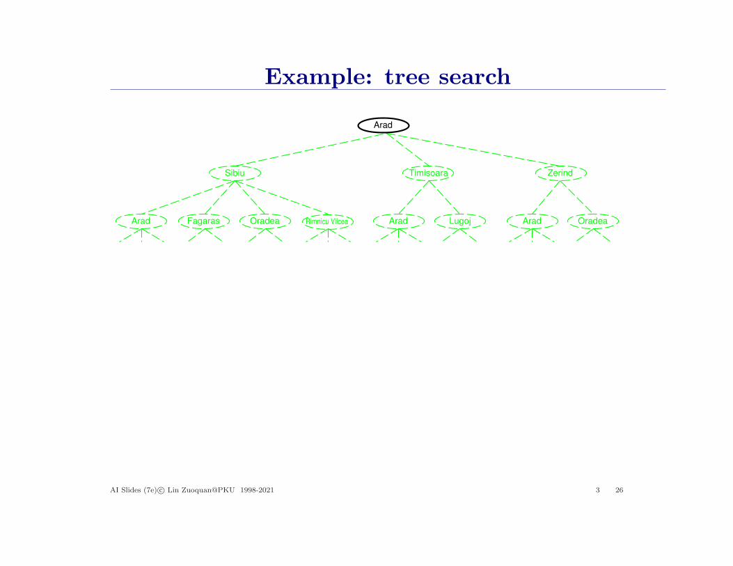
Example: tree search
Rimnicu Vilcea Lugoj
ZerindSibiu
Arad Fagaras Oradea
Timisoara
AradArad Oradea
Arad
AI Slides (7e) c© Lin Zuoquan@PKU 1998-2021 3 26

Example: tree search
Rimnicu Vilcea LugojArad Fagaras Oradea AradArad Oradea
Zerind
Arad
Sibiu Timisoara
AI Slides (7e) c© Lin Zuoquan@PKU 1998-2021 3 27
Example: tree search
Lugoj AradArad OradeaRimnicu Vilcea
Zerind
Arad
Sibiu
Arad Fagaras Oradea
Timisoara
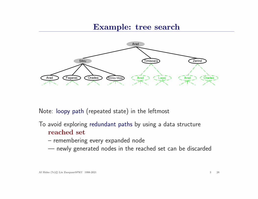
Note: loopy path (repeated state) in the leftmost
To avoid exploring redundant paths by using a data structurereached set
– remembering every expanded node— newly generated nodes in the reached set can be discarded
AI Slides (7e) c© Lin Zuoquan@PKU 1998-2021 3 28
Implementation: states vs. nodes
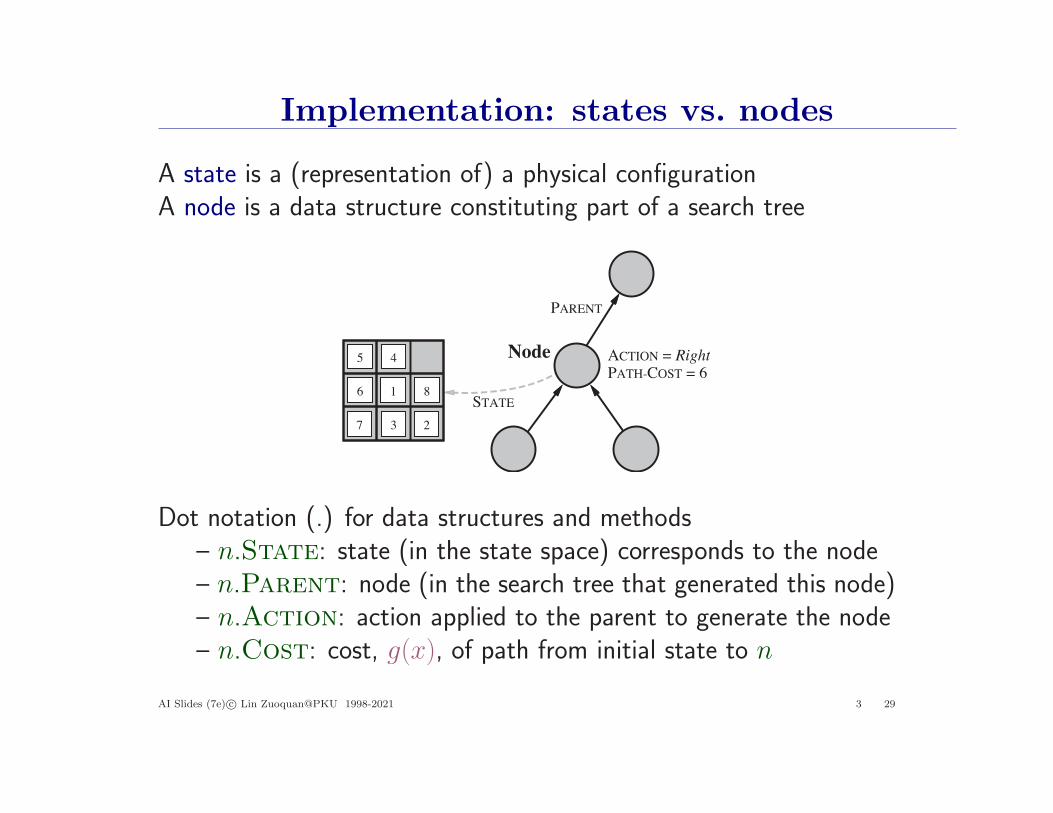
A state is a (representation of) a physical configurationA node is a data structure constituting part of a search tree
1
23
45
6
7
81
23
45
6
7
8
Node
STATE
PARENT
ACTION = RightPATH-COST = 6
Dot notation (.) for data structures and methods– n.State: state (in the state space) corresponds to the node– n.Parent: node (in the search tree that generated this node)– n.Action: action applied to the parent to generate the node– n.Cost: cost, g(x), of path from initial state to n
AI Slides (7e) c© Lin Zuoquan@PKU 1998-2021 3 29
Implementation: states vs. nodes
Queue: a data structure to store the frontier, with the operations• Is-Empty(frontier) returns true only if there are no nodes in
the frontier• Pop(frontier) removes the top node from the frontier and
returns it• Top(frontier) returns (but does not remove) the top node of
the frontier• Add(node, frontier) inserts node into its proper place in the
queue
Priority queue first pops the node with the minimum costFIFO (first-in-first-out) queue first pops the node that was added tothe queue firstLIFO (last-in-first-out) queue (a.k.a stack) pops first the most re-cently added node
AI Slides (7e) c© Lin Zuoquan@PKU 1998-2021 3 30
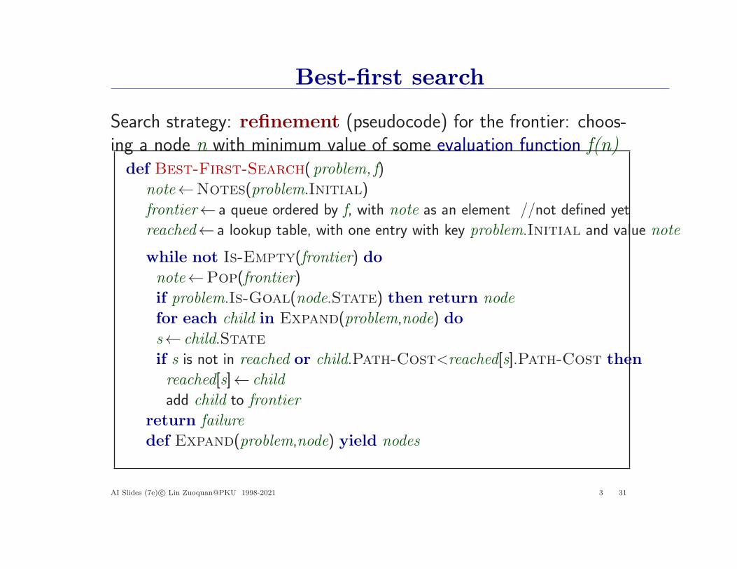
Best-first search
Search strategy: refinement (pseudocode) for the frontier: choos-ing a node n with minimum value of some evaluation function f(n)def Best-First-Search( problem, f)
note←Notes(problem.Initial)
frontier← a queue ordered by f, with note as an element //not defined yet
reached← a lookup table, with one entry with key problem.Initial and value note
while not Is-Empty(frontier) do
note←Pop(frontier)
if problem.Is-Goal(node.State) then return node
for each child in Expand(problem,node) do
s← child.State
if s is not in reached or child.Path-Cost<reached[s].Path-Cost then
reached[s]← child
add child to frontier
return failure
def Expand(problem,node) yield nodes
AI Slides (7e) c© Lin Zuoquan@PKU 1998-2021 3 31
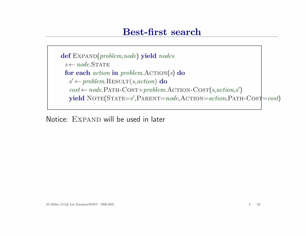
Best-first search
def Expand(problem,node) yield nodes
s← node.State
for each action in problem.Action(s) do
s′← problem.Result(s,action) do
cost← node.Path-Cost+problem.Action-Cost(s,action,s′)yield Note(State=s′,Parent=node,Action=action,Path-Cost=cost)
Notice: Expand will be used in later
AI Slides (7e) c© Lin Zuoquan@PKU 1998-2021 3 32

Search strategies
A strategy is defined by picking the order of node expansion
• Uninformed search• Informed search
Strategies are evaluated along the following dimensions:completeness—does it always find a solution if one exists?time complexity—number of nodes generated/expandedspace complexity—maximum number of nodes in memoryoptimality—does it always find a least-cost solution?
Time and space complexity are measured in terms ofb — maximum branching factor of the search treed — depth of the least-cost solutionm — maximum depth of the state space (may be ∞)
AI Slides (7e) c© Lin Zuoquan@PKU 1998-2021 3 33
Uninformed search strategies
Uninformed (blind) strategies use only the information availablein the problem definition
• Breadth-first search
• Uniform-cost search
• Depth-first search
• Depth-limited search
• Iterative deepening search
AI Slides (7e) c© Lin Zuoquan@PKU 1998-2021 3 34

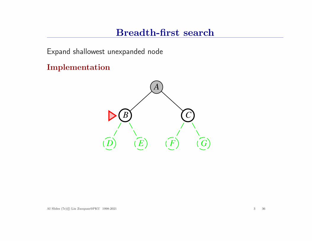
Breadth-first search
BFS: Expand shallowest unexpanded node
Implementation
frontier = FIFOA
B C
D E F G
AI Slides (7e) c© Lin Zuoquan@PKU 1998-2021 3 35
Breadth-first search
Expand shallowest unexpanded node
Implementation
A
B C
D E F G
AI Slides (7e) c© Lin Zuoquan@PKU 1998-2021 3 36
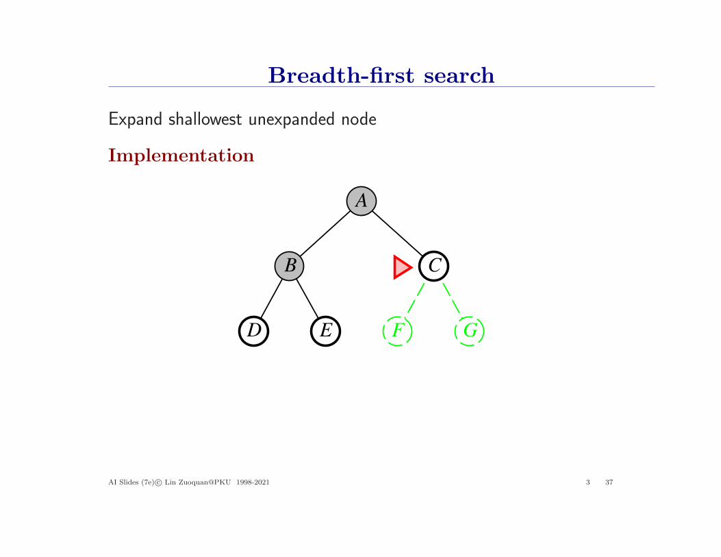
Breadth-first search
Expand shallowest unexpanded node
Implementation
A
B C
D E F G
AI Slides (7e) c© Lin Zuoquan@PKU 1998-2021 3 37
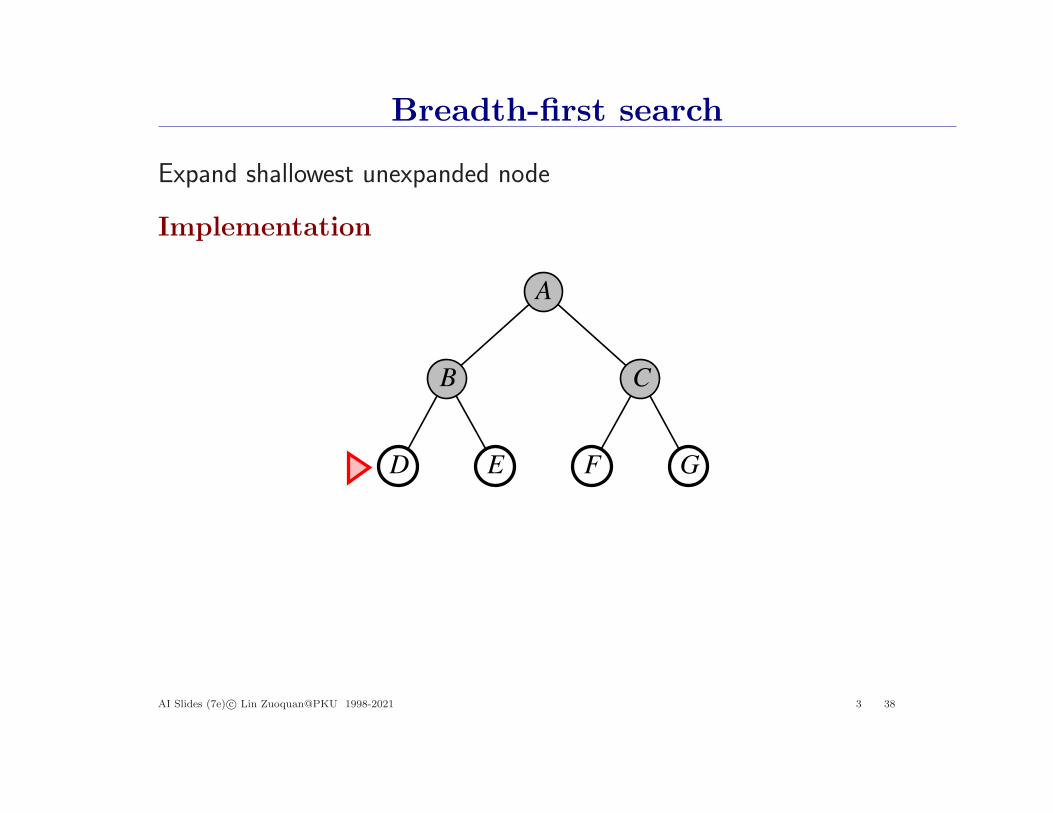
Breadth-first search
Expand shallowest unexpanded node
Implementation
A
B C
D E F G
AI Slides (7e) c© Lin Zuoquan@PKU 1998-2021 3 38

Breadth-first search
def Breadth-First-Search( problem)
node←Note(problem.Initial)
if problem.Is-Goal(node.State) then return node /* solution */
frontier← a FIFO queue with node as an element
reached←{problem.Initial}while not Is-Empty(frontier) do
node←Pop(frontier)
for each child in Expand(problem,node) do
s← child.State
if problem.Is-Goal(s) then return child /* solution */
if s is not in reached then
add s to reached
add child to frontier
return failure
AI Slides (7e) c© Lin Zuoquan@PKU 1998-2021 3 39

Properties of breadth-first search
Complete??
AI Slides (7e) c© Lin Zuoquan@PKU 1998-2021 3 40
Properties of breadth-first search
Complete?? Yes (if b is finite)
Time??
AI Slides (7e) c© Lin Zuoquan@PKU 1998-2021 3 41

Properties of breadth-first search
Complete?? Yes (if b is finite)
Time?? 1 + b + b2 + b3 + . . . + bd + b(bd − 1) = O(bd+1)i.e., exp. in d
Space??
AI Slides (7e) c© Lin Zuoquan@PKU 1998-2021 3 42
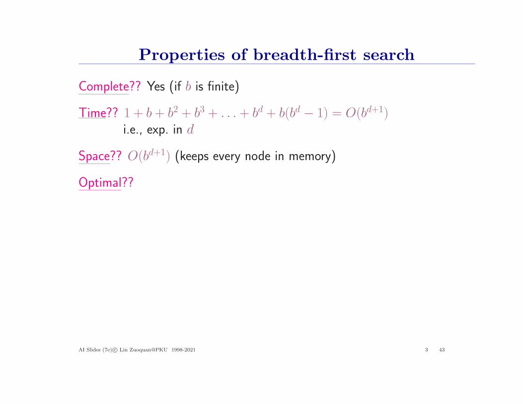
Properties of breadth-first search
Complete?? Yes (if b is finite)
Time?? 1 + b + b2 + b3 + . . . + bd + b(bd − 1) = O(bd+1)i.e., exp. in d
Space?? O(bd+1) (keeps every node in memory)
Optimal??
AI Slides (7e) c© Lin Zuoquan@PKU 1998-2021 3 43
Properties of breadth-first search
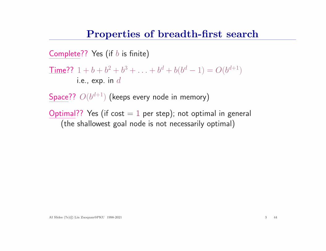
Complete?? Yes (if b is finite)
Time?? 1 + b + b2 + b3 + . . . + bd + b(bd − 1) = O(bd+1)i.e., exp. in d
Space?? O(bd+1) (keeps every node in memory)
Optimal?? Yes (if cost = 1 per step); not optimal in general(the shallowest goal node is not necessarily optimal)
AI Slides (7e) c© Lin Zuoquan@PKU 1998-2021 3 44
Properties of breadth-first search
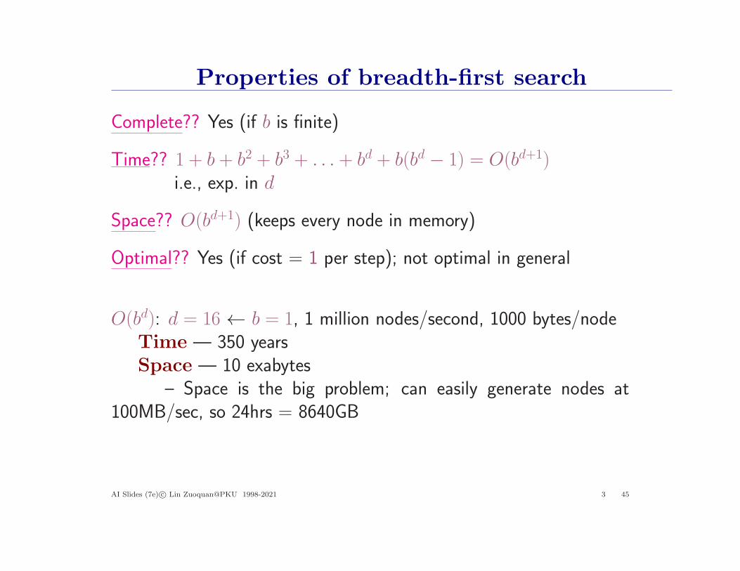
Complete?? Yes (if b is finite)
Time?? 1 + b + b2 + b3 + . . . + bd + b(bd − 1) = O(bd+1)i.e., exp. in d
Space?? O(bd+1) (keeps every node in memory)
Optimal?? Yes (if cost = 1 per step); not optimal in general
O(bd): d = 16 ← b = 1, 1 million nodes/second, 1000 bytes/nodeTime — 350 yearsSpace — 10 exabytes
– Space is the big problem; can easily generate nodes at100MB/sec, so 24hrs = 8640GB
AI Slides (7e) c© Lin Zuoquan@PKU 1998-2021 3 45
Python: search classes∗
"""
Search
Create classes of problems and problem instances, and solve them with calls to the various search functions.
"""
import sys
from collections import deque
from utils import *
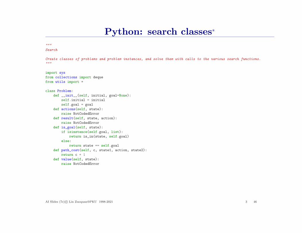
class Problem:
def __init__(self, initial, goal=None):
self.initial = initial
self.goal = goal
def actions(self, state):
raise NotCodedError
def result(self, state, action):
raise NotCodedError
def is_goal(self, state):
if isinstance(self.goal, list):
return is_in(state, self.goal)
else:
return state == self.goal
def path_cost(self, c, state1, action, state2):
return c + 1
def value(self, state):
raise NotCodedError
AI Slides (7e) c© Lin Zuoquan@PKU 1998-2021 3 46

Python: search classes∗
class Node:
"""A node in a search tree."""
def __init__(self, state, parent=None, action=None, path_cost=0):
self.state = state
self.parent = parent
self.action = action
self.path_cost = path_cost
self.depth = 0
if parent:
self.depth = parent.depth + 1
def __repr__(self):
return "<Node {}>".format(self.state)
def __lt__(self, node):
return self.state < node.state
def expand(self, problem):
return [self.child_node(problem, action)
for action in problem.actions(self.state)]
def child_node(self, problem, action):
next_state = problem.result(self.state, action)
next_node = Node(next_state, self, action, problem.path_cost(self.path_cost, self.state, action, next_state))
return next_node
def solution(self):
return [node.action for node in self.path()[1:]]
AI Slides (7e) c© Lin Zuoquan@PKU 1998-2021 3 47
Python: search classes∗
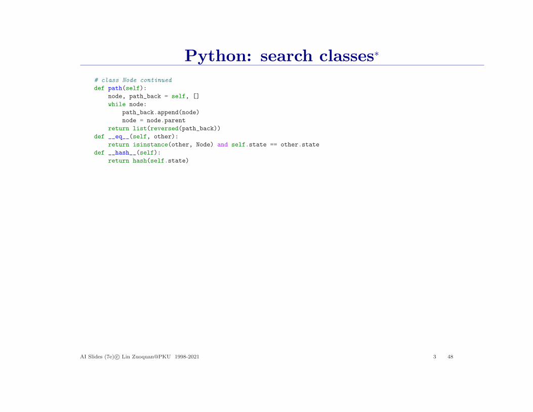
# class Node continued
def path(self):
node, path_back = self, []
while node:
path_back.append(node)
node = node.parent
return list(reversed(path_back))
def __eq__(self, other):
return isinstance(other, Node) and self.state == other.state
def __hash__(self):
return hash(self.state)
AI Slides (7e) c© Lin Zuoquan@PKU 1998-2021 3 48

Python: breadth-first search∗
"""
BFS
Implemente the pseudocode by calling function.
"""
def breadth_first_search(problem):
frontier = deque([Node(problem.initial)]) # FIFO queue
while frontier:
node = frontier.popleft()
if problem.is_goal(node.state):
return node
frontier.extend(node.expand(problem))
return None
Is it possible to have a tool to translate the pseudocode to Python??— Refer to Natural Language Understanding
AI Slides (7e) c© Lin Zuoquan@PKU 1998-2021 3 49
Uniform-cost search
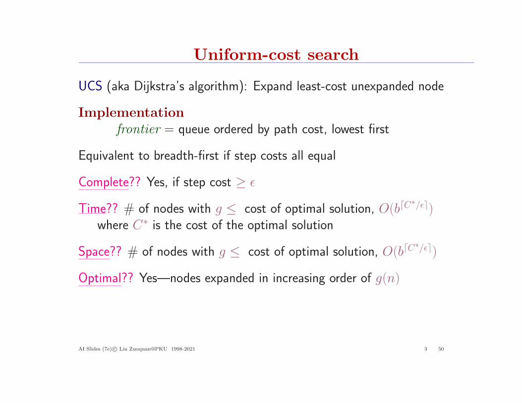
UCS (aka Dijkstra’s algorithm): Expand least-cost unexpanded node
Implementation
frontier = queue ordered by path cost, lowest first
Equivalent to breadth-first if step costs all equal
Complete?? Yes, if step cost ≥ ǫ
Time?? # of nodes with g ≤ cost of optimal solution, O(b⌈C∗/ǫ⌉)
where C∗ is the cost of the optimal solution
Space?? # of nodes with g ≤ cost of optimal solution, O(b⌈C∗/ǫ⌉)
Optimal?? Yes—nodes expanded in increasing order of g(n)
AI Slides (7e) c© Lin Zuoquan@PKU 1998-2021 3 50
Uniform-cost search
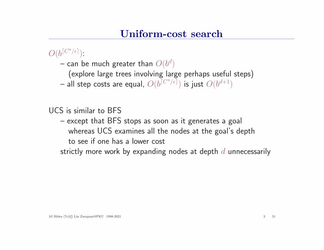
O(b⌈C∗/ǫ⌉):
– can be much greater than O(bd)(explore large trees involving large perhaps useful steps)
– all step costs are equal, O(b⌈C∗/ǫ⌉) is just O(bd+1)
UCS is similar to BFS– except that BFS stops as soon as it generates a goalwhereas UCS examines all the nodes at the goal’s depthto see if one has a lower cost
strictly more work by expanding nodes at depth d unnecessarily
AI Slides (7e) c© Lin Zuoquan@PKU 1998-2021 3 51
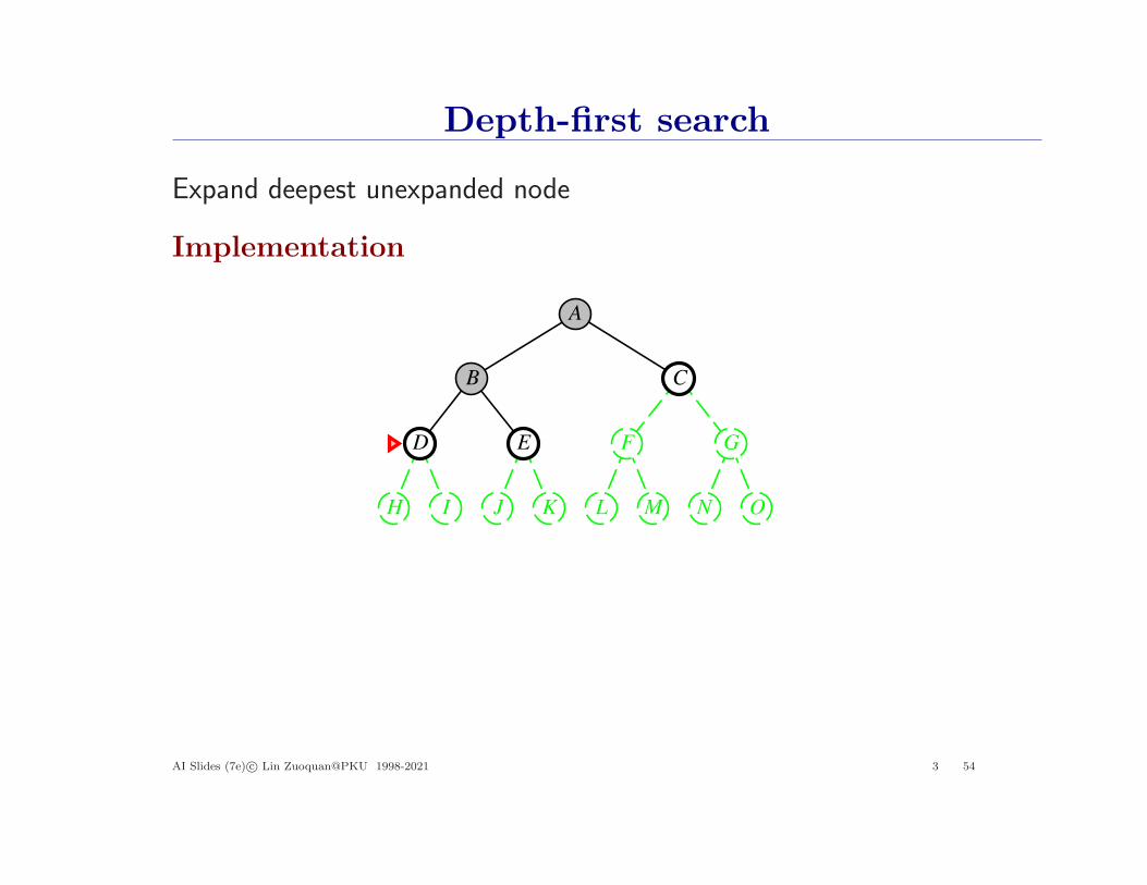
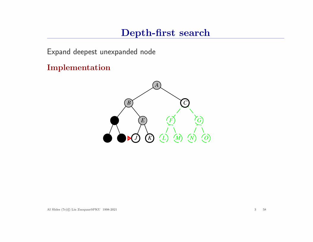
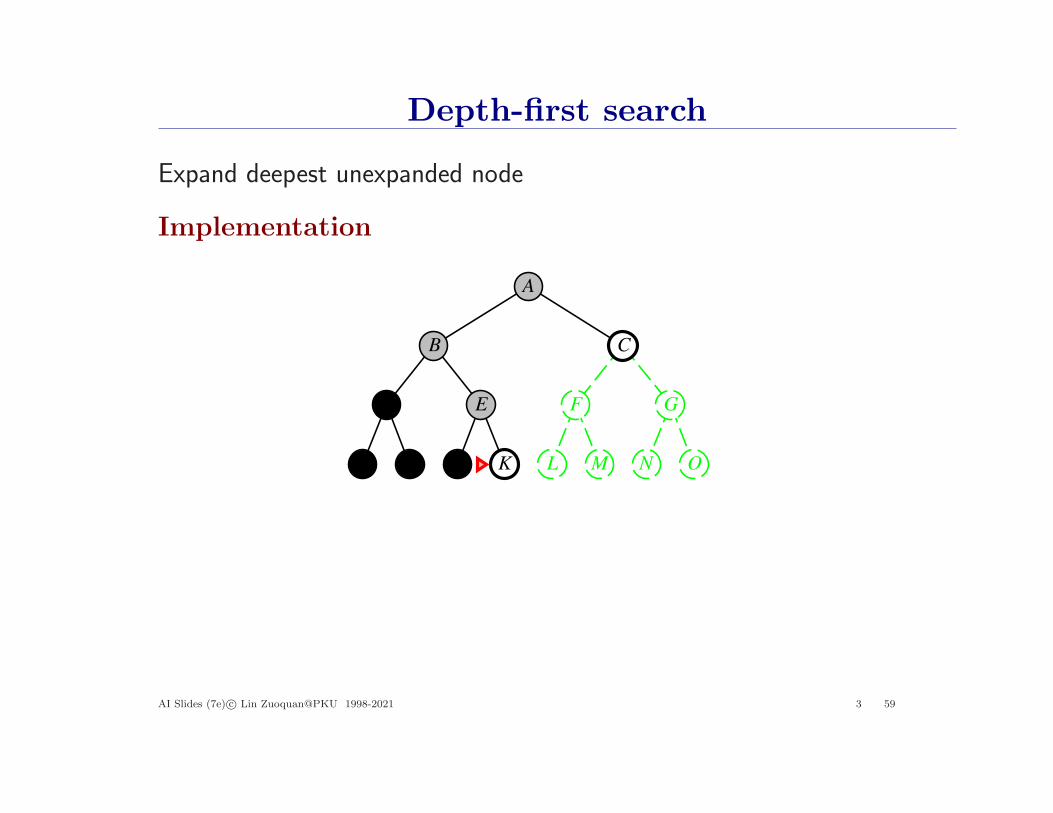
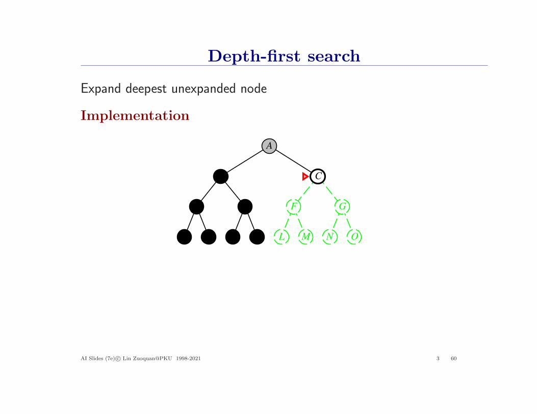
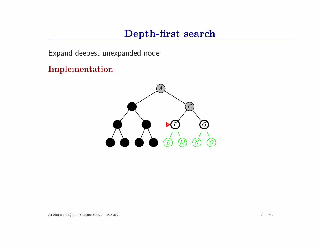
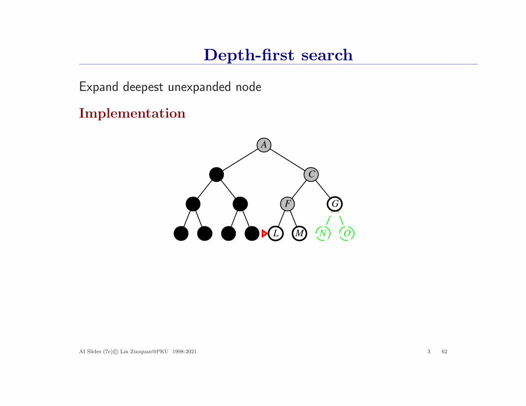
Depth-first search
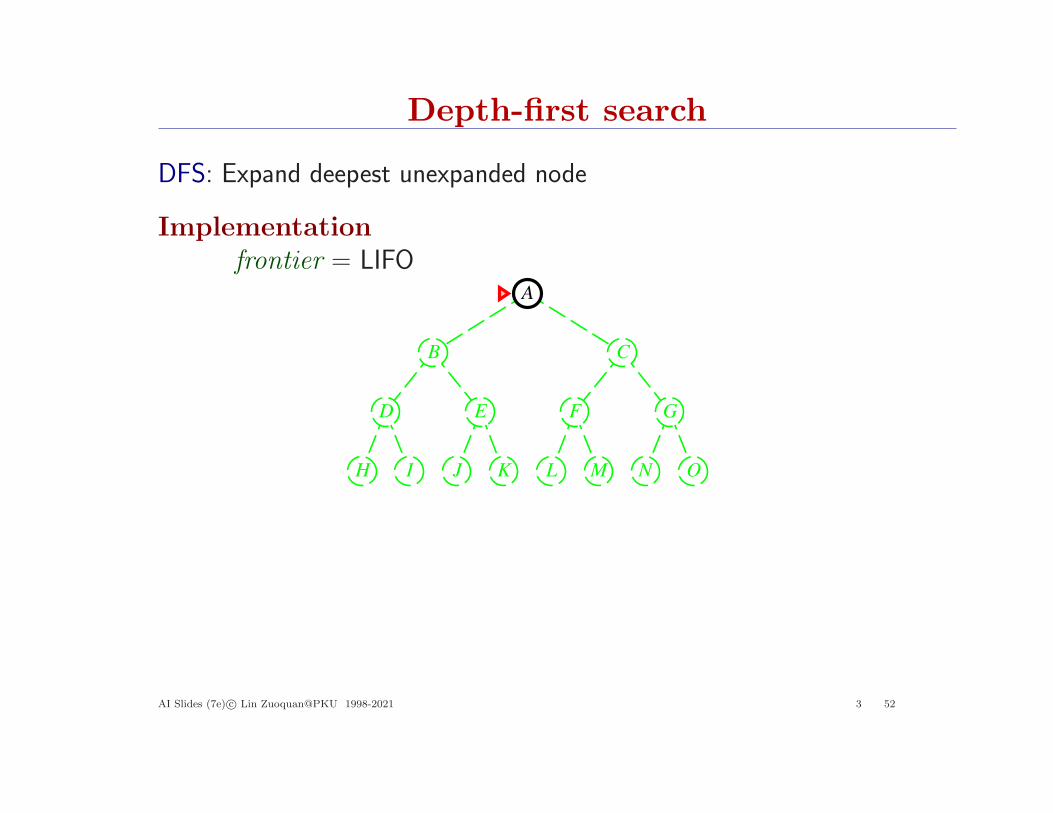
DFS: Expand deepest unexpanded node
Implementation
frontier = LIFOA
B C
D E F G
H I J K L M N O
AI Slides (7e) c© Lin Zuoquan@PKU 1998-2021 3 52
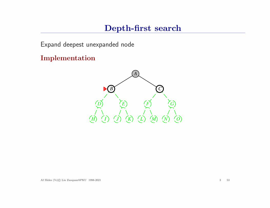
Depth-first search
Expand deepest unexpanded node
Implementation
A
B C
D E F G
H I J K L M N O
AI Slides (7e) c© Lin Zuoquan@PKU 1998-2021 3 53
Depth-first search
Expand deepest unexpanded node
Implementation
A
B C
D E F G
H I J K L M N O
AI Slides (7e) c© Lin Zuoquan@PKU 1998-2021 3 54
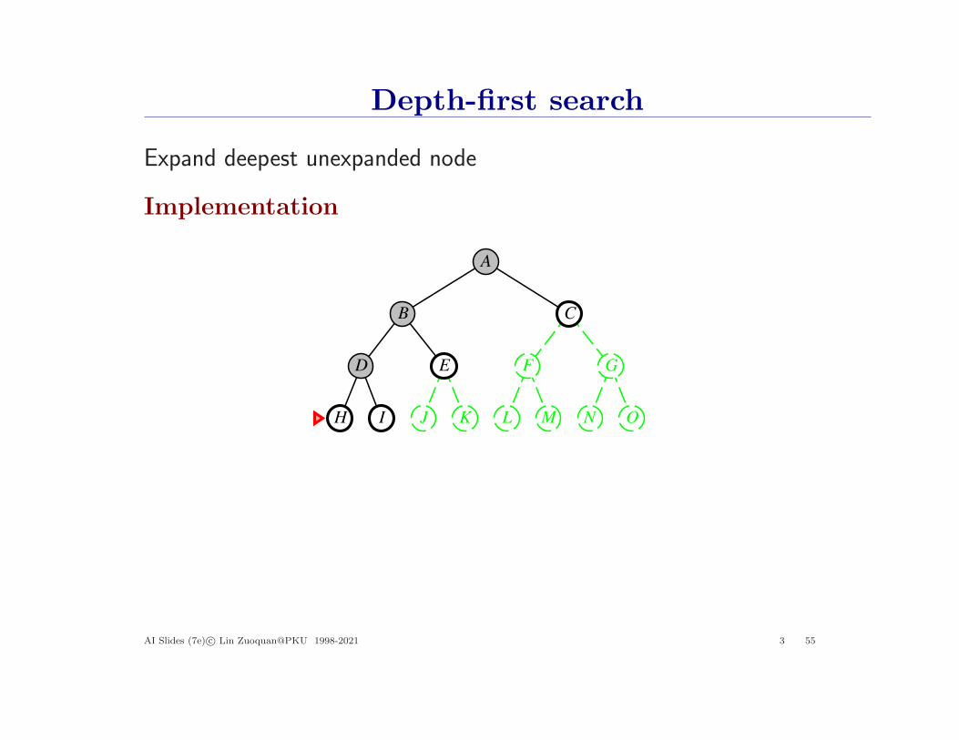
Depth-first search
Expand deepest unexpanded node
Implementation
A
B C
D E F G
H I J K L M N O
AI Slides (7e) c© Lin Zuoquan@PKU 1998-2021 3 55
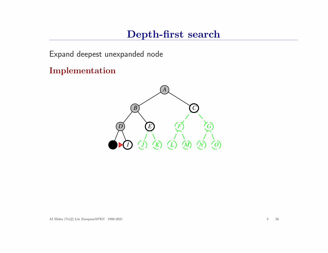
Depth-first search
Expand deepest unexpanded node
Implementation
A
B C
D E F G
H I J K L M N O
AI Slides (7e) c© Lin Zuoquan@PKU 1998-2021 3 56
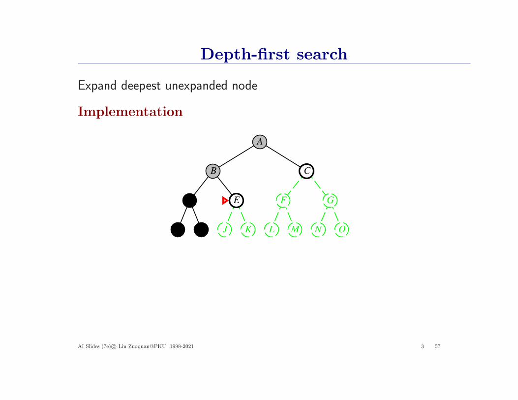
Depth-first search
Expand deepest unexpanded node
Implementation
A
B C
D E F G
H I J K L M N O
AI Slides (7e) c© Lin Zuoquan@PKU 1998-2021 3 57
Depth-first search
Expand deepest unexpanded node
Implementation
A
B C
D E F G
H I J K L M N O
AI Slides (7e) c© Lin Zuoquan@PKU 1998-2021 3 58
Depth-first search
Expand deepest unexpanded node
Implementation
A
B C
D E F G
H I J K L M N O
AI Slides (7e) c© Lin Zuoquan@PKU 1998-2021 3 59
Depth-first search
Expand deepest unexpanded node
Implementation
A
B C
D E F G
H I J K L M N O
AI Slides (7e) c© Lin Zuoquan@PKU 1998-2021 3 60
Depth-first search
Expand deepest unexpanded node
Implementation
A
B C
D E F G
H I J K L M N O
AI Slides (7e) c© Lin Zuoquan@PKU 1998-2021 3 61
Depth-first search
Expand deepest unexpanded node
Implementation
A
B C
D E F G
H I J K L M N O
AI Slides (7e) c© Lin Zuoquan@PKU 1998-2021 3 62

Depth-first search
Expand deepest unexpanded node
Implementation
A
B C
D E F G
H I J K L M N O
AI Slides (7e) c© Lin Zuoquan@PKU 1998-2021 3 63

Properties of depth-first search
Complete??
AI Slides (7e) c© Lin Zuoquan@PKU 1998-2021 3 64

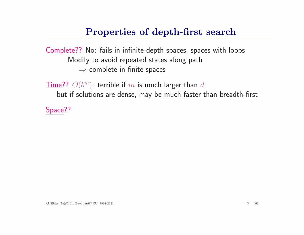
Properties of depth-first search
Complete?? No: fails in infinite-depth spaces, spaces with loopsModify to avoid repeated states along path⇒ complete in finite spaces
Time??
AI Slides (7e) c© Lin Zuoquan@PKU 1998-2021 3 65
Properties of depth-first search
Complete?? No: fails in infinite-depth spaces, spaces with loopsModify to avoid repeated states along path⇒ complete in finite spaces
Time?? O(bm): terrible if m is much larger than dbut if solutions are dense, may be much faster than breadth-first
Space??
AI Slides (7e) c© Lin Zuoquan@PKU 1998-2021 3 66
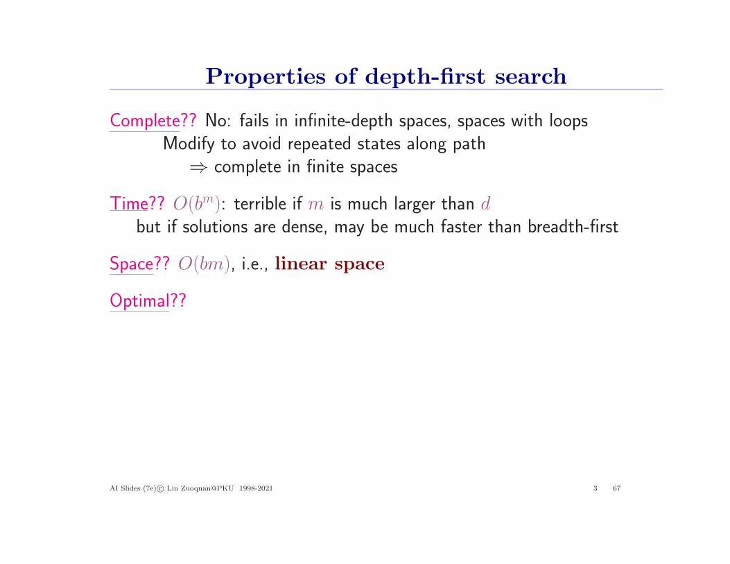
Properties of depth-first search
Complete?? No: fails in infinite-depth spaces, spaces with loopsModify to avoid repeated states along path⇒ complete in finite spaces
Time?? O(bm): terrible if m is much larger than dbut if solutions are dense, may be much faster than breadth-first
Space?? O(bm), i.e., linear space
Optimal??
AI Slides (7e) c© Lin Zuoquan@PKU 1998-2021 3 67
Properties of depth-first search
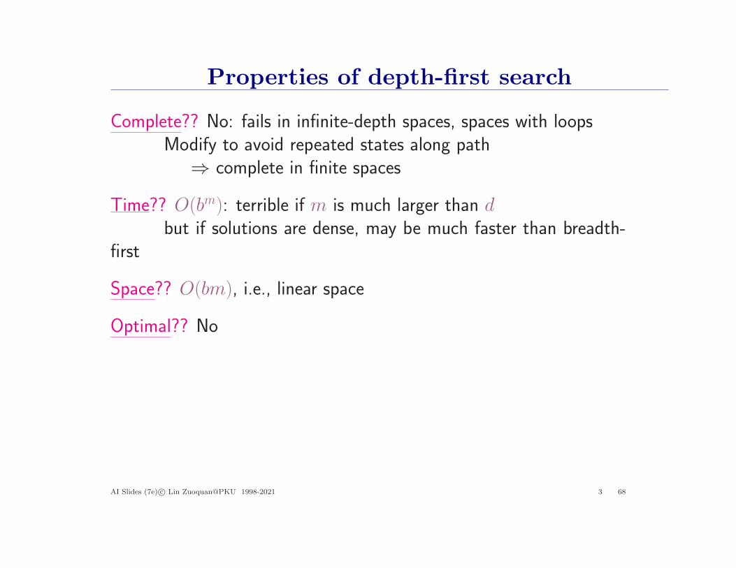
Complete?? No: fails in infinite-depth spaces, spaces with loopsModify to avoid repeated states along path⇒ complete in finite spaces
Time?? O(bm): terrible if m is much larger than dbut if solutions are dense, may be much faster than breadth-
first
Space?? O(bm), i.e., linear space
Optimal?? No
AI Slides (7e) c© Lin Zuoquan@PKU 1998-2021 3 68
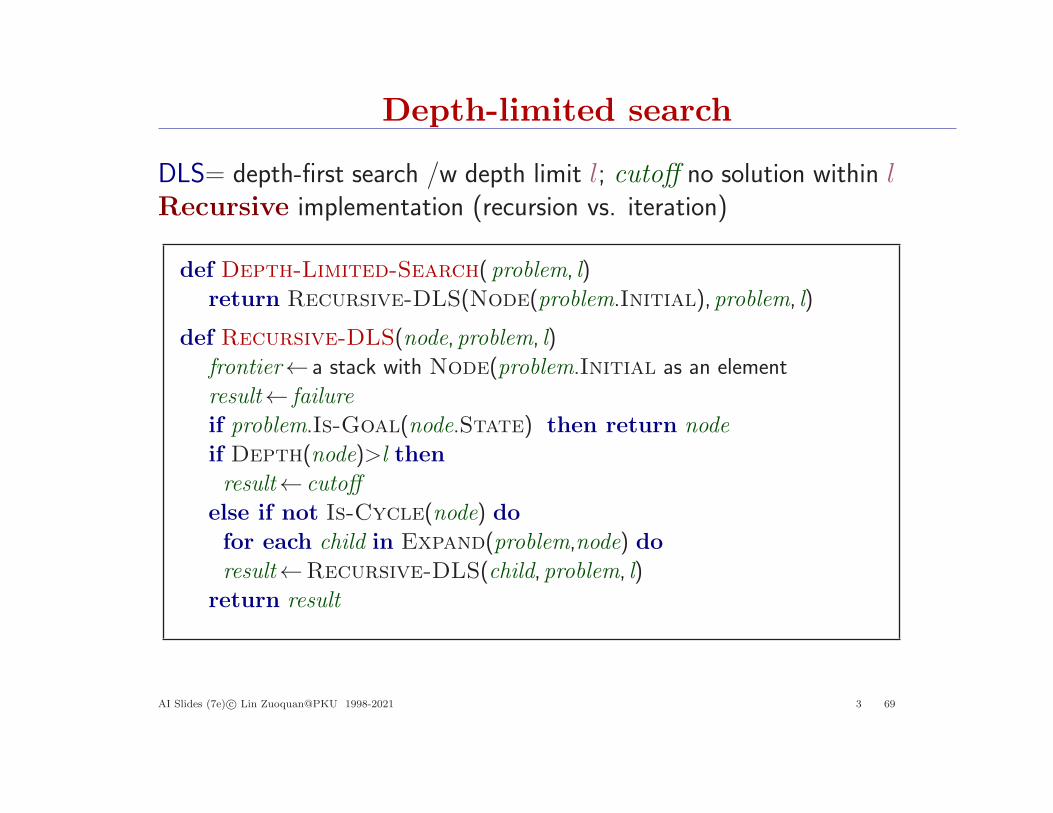
Depth-limited search
DLS= depth-first search /w depth limit l; cutoff no solution within lRecursive implementation (recursion vs. iteration)
def Depth-Limited-Search( problem, l)
return Recursive-DLS(Node(problem.Initial),problem, l)
def Recursive-DLS(node,problem, l)
frontier← a stack with Node(problem.Initial as an element
result← failure
if problem.Is-Goal(node.State) then return node
if Depth(node)>l then
result← cutoff
else if not Is-Cycle(node) do
for each child in Expand(problem,node) do
result←Recursive-DLS(child,problem, l)
return result
AI Slides (7e) c© Lin Zuoquan@PKU 1998-2021 3 69

Iterative deepening search
IDS repeatedly applies DLS with increasing limits
def Iterative-Deepening-Search( problem)
for depth=0 to ∞ do
result←Depth-Limited-Search( problem, depth)
if result 6= cutoff then return result
AI Slides (7e) c© Lin Zuoquan@PKU 1998-2021 3 70
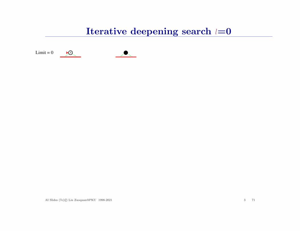
Iterative deepening search l=0
Limit = 0 A A
AI Slides (7e) c© Lin Zuoquan@PKU 1998-2021 3 71

Iterative deepening search l = 1
Limit = 1 A
B C
A
B C
A
B C
A
B C
AI Slides (7e) c© Lin Zuoquan@PKU 1998-2021 3 72
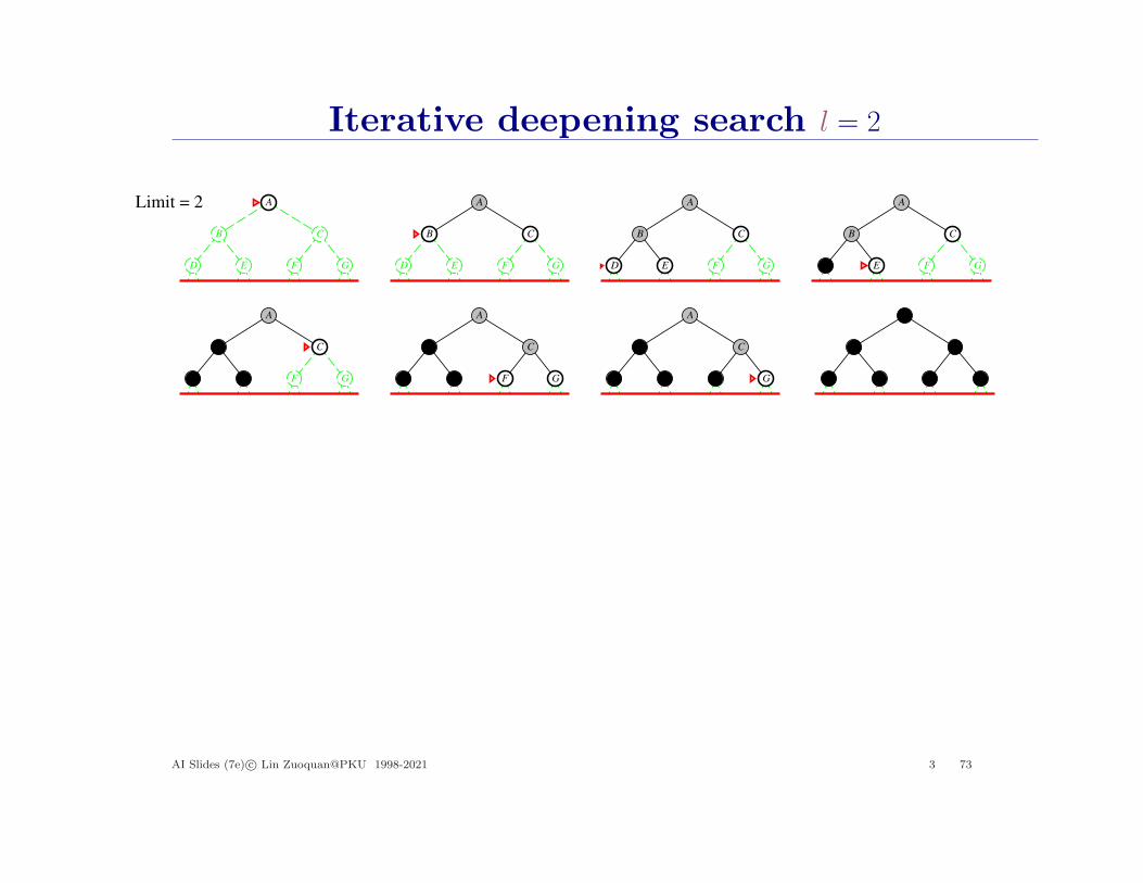
Iterative deepening search l = 2
Limit = 2 A
B C
D E F G
A
B C
D E F G
A
B C
D E F G
A
B C
D E F G
A
B C
D E F G
A
B C
D E F G
A
B C
D E F G
A
B C
D E F G
AI Slides (7e) c© Lin Zuoquan@PKU 1998-2021 3 73

Iterative deepening search l = 3
Limit = 3
A
B C
D E F G
H I J K L M N O
A
B C
D E F G
H I J K L M N O
A
B C
D E F G
H I J K L M N O
A
B C
D E F G
H I J K L M N O
A
B C
D E F G
H I J K L M N O
A
B C
D E F G
H I J K L M N O
A
B C
D E F G
H I J K L M N O
A
B C
D E F G
H I J K L M N O
A
B C
D E F G
H I J K L M N O
A
B C
D E F G
H I J K L M N O
A
B C
D E F G
H J K L M N OI
A
B C
D E F G
H I J K L M N O
AI Slides (7e) c© Lin Zuoquan@PKU 1998-2021 3 74
Properties of iterative deepening search
Complete??
AI Slides (7e) c© Lin Zuoquan@PKU 1998-2021 3 75
Properties of iterative deepening search
Complete?? Yes
Time??
AI Slides (7e) c© Lin Zuoquan@PKU 1998-2021 3 76
Properties of iterative deepening search
Complete?? Yes
Time?? (d + 1)b0 + db1 + (d− 1)b2 + . . . + bd = O(bd)
Space??
AI Slides (7e) c© Lin Zuoquan@PKU 1998-2021 3 77
Properties of iterative deepening search
Complete?? Yes
Time?? (d + 1)b0 + db1 + (d− 1)b2 + . . . + bd = O(bd)
Space?? O(bd)
Optimal??
AI Slides (7e) c© Lin Zuoquan@PKU 1998-2021 3 78

Properties of iterative deepening search
Complete?? Yes
Time?? (d + 1)b0 + db1 + (d− 1)b2 + . . . + bd = O(bd)
Space?? O(bd)
Optimal?? Yes, if step cost = 1Can be modified to explore uniform-cost tree
Numerical comparison for b = 10 and d = 5, solution at far rightleaf:
N(IDS) = 50 + 400 + 3, 000 + 20, 000 + 100, 000 = 123, 450
N(BFS) = 10 + 100 + 1, 000 + 10, 000 + 100, 000 + 999, 990 = 111, 100
IDS does better because other nodes at depth d are not expandedBFS can be modified to apply goal test when a node is generated
AI Slides (7e) c© Lin Zuoquan@PKU 1998-2021 3 79
Bidirection search∗
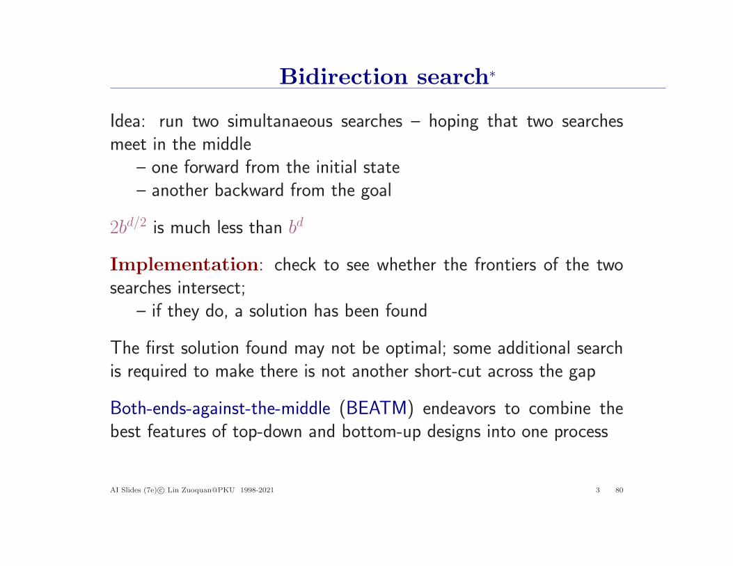
Idea: run two simultanaeous searches – hoping that two searchesmeet in the middle
– one forward from the initial state– another backward from the goal
2bd/2 is much less than bd
Implementation: check to see whether the frontiers of the twosearches intersect;
– if they do, a solution has been found
The first solution found may not be optimal; some additional searchis required to make there is not another short-cut across the gap
Both-ends-against-the-middle (BEATM) endeavors to combine thebest features of top-down and bottom-up designs into one process
AI Slides (7e) c© Lin Zuoquan@PKU 1998-2021 3 80
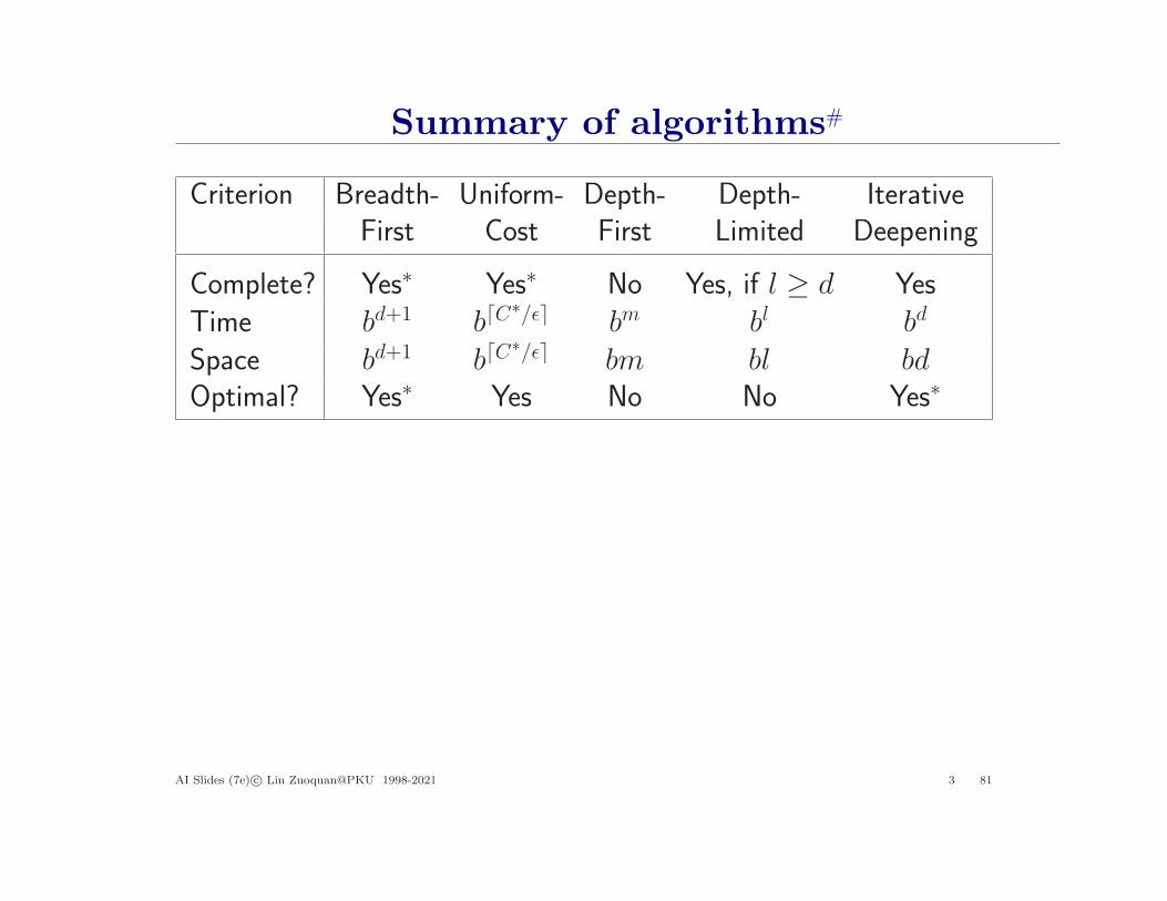
Summary of algorithms#
Criterion Breadth- Uniform- Depth- Depth- IterativeFirst Cost First Limited Deepening
Complete? Yes∗ Yes∗ No Yes, if l ≥ d YesTime bd+1 b⌈C
∗/ǫ⌉ bm bl bd
Space bd+1 b⌈C∗/ǫ⌉ bm bl bd
Optimal? Yes∗ Yes No No Yes∗
AI Slides (7e) c© Lin Zuoquan@PKU 1998-2021 3 81

Graph search: repeated states∗
Graph ⇒ Tree
Failure to detect repeated states can turn a linear problem into anexponential one
A
B
C
D
A
BB
CCCC
d + 1 states space ⇒ 2d paths
All the tree-search versions of algorithms can be extended to thegraph-search versions by checking the repeated states
AI Slides (7e) c© Lin Zuoquan@PKU 1998-2021 3 82

Graph search∗
def Graph-Search( problem)
initialize the frontier using the initial state of problem
initialize the reached set to empty
loop do
if the frontier is empty then return failure
choose a leaf node and remove it from the frontier
if the node contains a goal state then return node
add node to the reached set
expand the chosen node and add the resulting nodes to the frontier
only if not in the frontier or reached set
Note: using reached set to avoid exploring redundant paths
AI Slides (7e) c© Lin Zuoquan@PKU 1998-2021 3 83
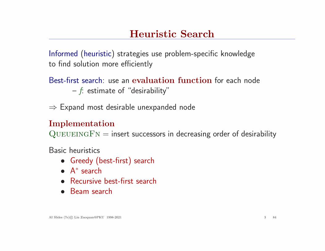
Heuristic Search
Informed (heuristic) strategies use problem-specific knowledgeto find solution more efficiently
Best-first search: use an evaluation function for each node– f: estimate of “desirability”
⇒ Expand most desirable unexpanded node
Implementation
QueueingFn = insert successors in decreasing order of desirability
Basic heuristics• Greedy (best-first) search• A∗ search• Recursive best-first search• Beam search
AI Slides (7e) c© Lin Zuoquan@PKU 1998-2021 3 84
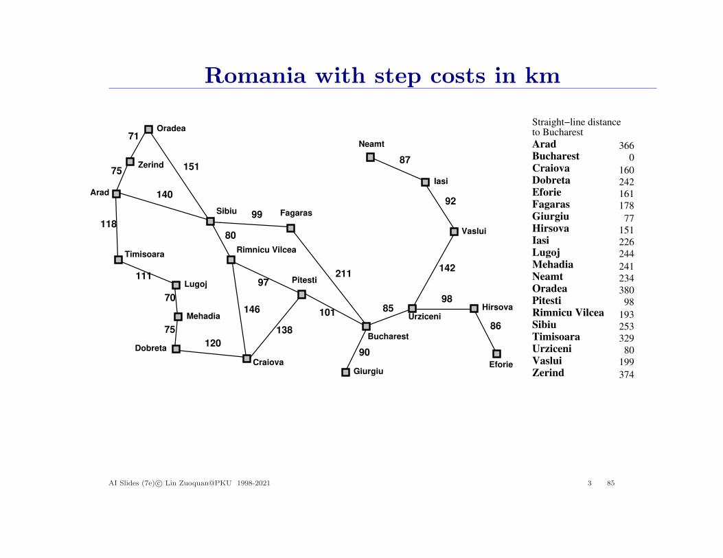
Romania with step costs in km
Bucharest
Giurgiu
Urziceni
Hirsova
Eforie
NeamtOradea
Zerind
Arad
Timisoara
LugojMehadia
DobretaCraiova
Sibiu
Fagaras
PitestiRimnicu Vilcea
Vaslui
Iasi
Straight−line distanceto Bucharest
0
160
242
161
77
151
241
366
193
178
253
329
80
199
244
380
226
234
374
98
Giurgiu
UrziceniHirsova
Eforie
Neamt
Oradea
Zerind
Arad
Timisoara
Lugoj
Mehadia
Dobreta
Craiova
Sibiu Fagaras
Pitesti
Vaslui
Iasi
Rimnicu Vilcea
Bucharest
71
75
118
111
70
75
120
151
140
99
80
97
101
211
138
146 85
90
98
142
92
87
86
AI Slides (7e) c© Lin Zuoquan@PKU 1998-2021 3 85
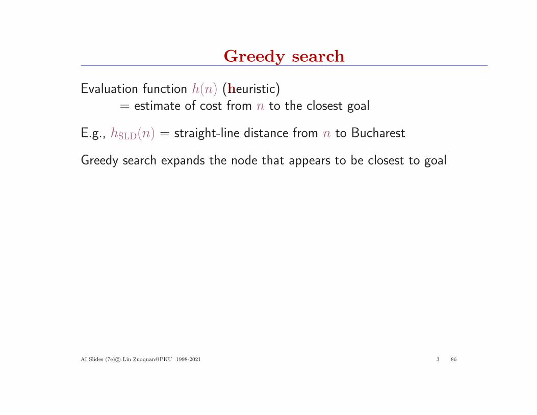
Greedy search
Evaluation function h(n) (heuristic)= estimate of cost from n to the closest goal
E.g., hSLD(n) = straight-line distance from n to Bucharest
Greedy search expands the node that appears to be closest to goal
AI Slides (7e) c© Lin Zuoquan@PKU 1998-2021 3 86
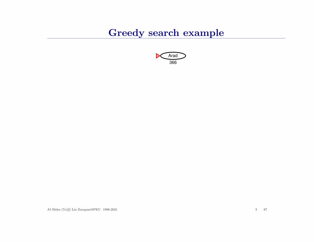
Greedy search example
Arad
366
AI Slides (7e) c© Lin Zuoquan@PKU 1998-2021 3 87
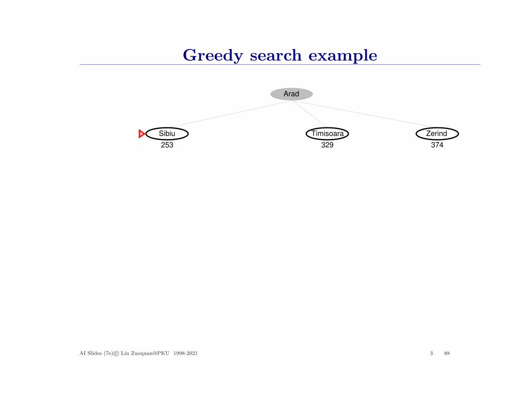
Greedy search example
Zerind
Arad
Sibiu Timisoara
253 329 374
AI Slides (7e) c© Lin Zuoquan@PKU 1998-2021 3 88

Greedy search example
Rimnicu Vilcea
Zerind
Arad
Sibiu
Arad Fagaras Oradea
Timisoara
329 374
366 176 380 193
AI Slides (7e) c© Lin Zuoquan@PKU 1998-2021 3 89
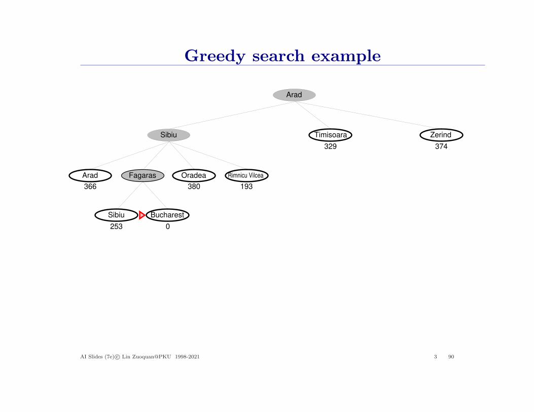
Greedy search example
Rimnicu Vilcea
Zerind
Arad
Sibiu
Arad Fagaras Oradea
Timisoara
Sibiu Bucharest
329 374
366 380 193
253 0
AI Slides (7e) c© Lin Zuoquan@PKU 1998-2021 3 90
Properties of greedy search
Complete??
AI Slides (7e) c© Lin Zuoquan@PKU 1998-2021 3 91
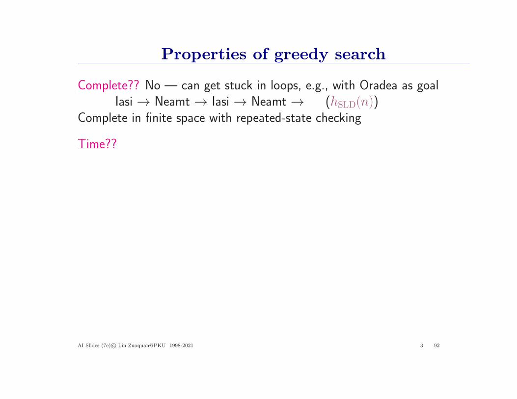
Properties of greedy search
Complete?? No — can get stuck in loops, e.g., with Oradea as goalIasi → Neamt → Iasi → Neamt → (hSLD(n))
Complete in finite space with repeated-state checking
Time??
AI Slides (7e) c© Lin Zuoquan@PKU 1998-2021 3 92
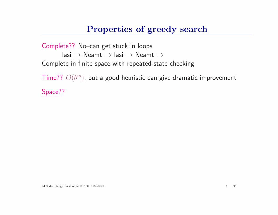
Properties of greedy search
Complete?? No–can get stuck in loopsIasi → Neamt → Iasi → Neamt →
Complete in finite space with repeated-state checking
Time?? O(bm), but a good heuristic can give dramatic improvement
Space??
AI Slides (7e) c© Lin Zuoquan@PKU 1998-2021 3 93
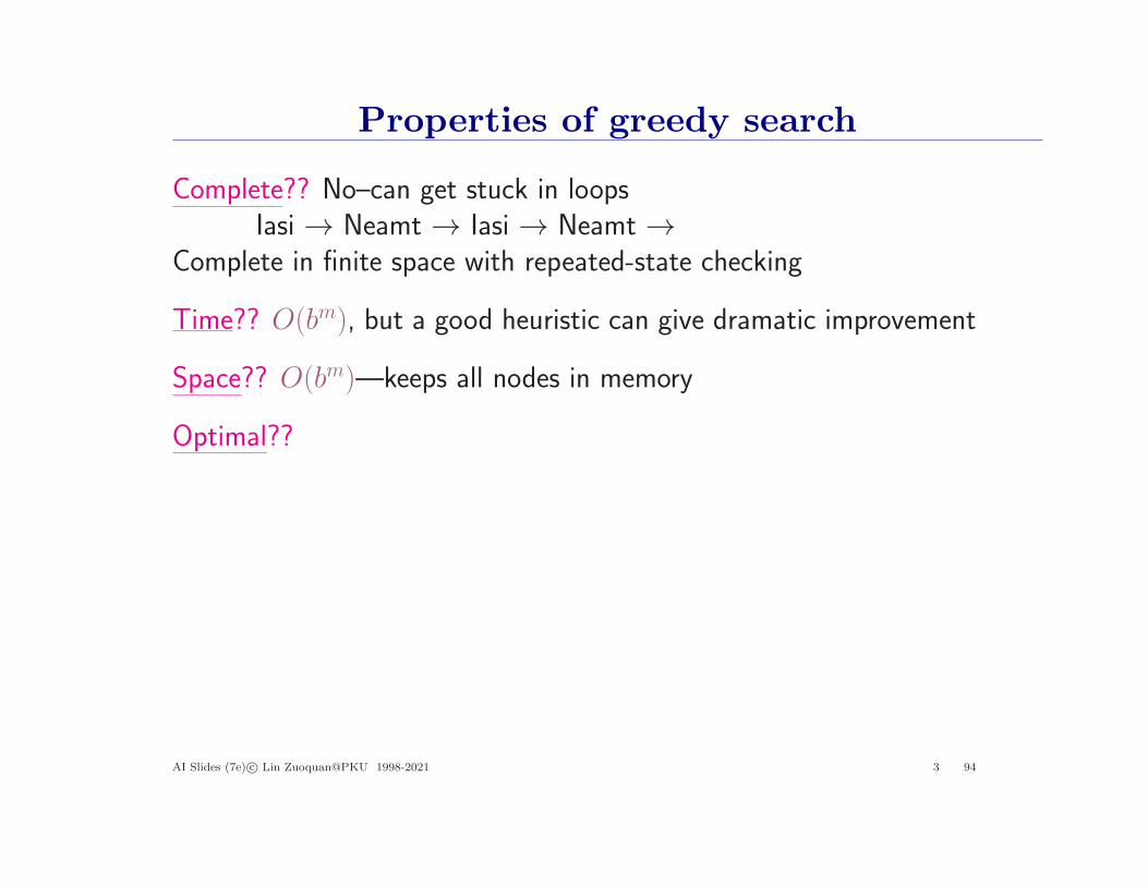
Properties of greedy search
Complete?? No–can get stuck in loopsIasi → Neamt → Iasi → Neamt →
Complete in finite space with repeated-state checking
Time?? O(bm), but a good heuristic can give dramatic improvement
Space?? O(bm)—keeps all nodes in memory
Optimal??
AI Slides (7e) c© Lin Zuoquan@PKU 1998-2021 3 94
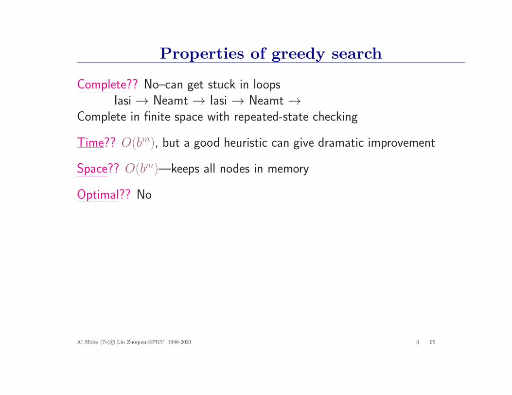
Properties of greedy search
Complete?? No–can get stuck in loopsIasi → Neamt → Iasi → Neamt →
Complete in finite space with repeated-state checking
Time?? O(bm), but a good heuristic can give dramatic improvement
Space?? O(bm)—keeps all nodes in memory
Optimal?? No
AI Slides (7e) c© Lin Zuoquan@PKU 1998-2021 3 95

A∗ search
Idea: avoid expanding paths that are already expensive
Evaluation function f (n) = g(n) + h(n)
g(n) = cost so far to reach nh(n) = estimated cost to goal from nf (n) = estimated total cost of path through n to goal
Algorithm: identical to Uniform-Cost-Search except for using g + hinstead of g
A∗ search uses an admissible heuristici.e., h(n) ≤ h∗(n) where h∗(n) is the true cost from n(Also require h(n) ≥ 0, so h(G) = 0 for any goal G)
E.g., hSLD(n) never overestimates the actual road distance
Theorem: A∗ search is optimal
AI Slides (7e) c© Lin Zuoquan@PKU 1998-2021 3 96
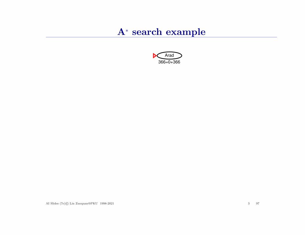
A∗ search example
Arad
366=0+366
AI Slides (7e) c© Lin Zuoquan@PKU 1998-2021 3 97
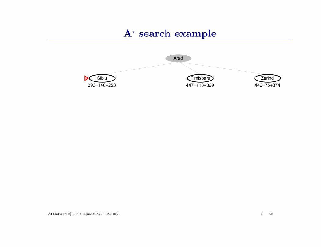
A∗ search example
Zerind
Arad
Sibiu Timisoara
447=118+329 449=75+374393=140+253
AI Slides (7e) c© Lin Zuoquan@PKU 1998-2021 3 98
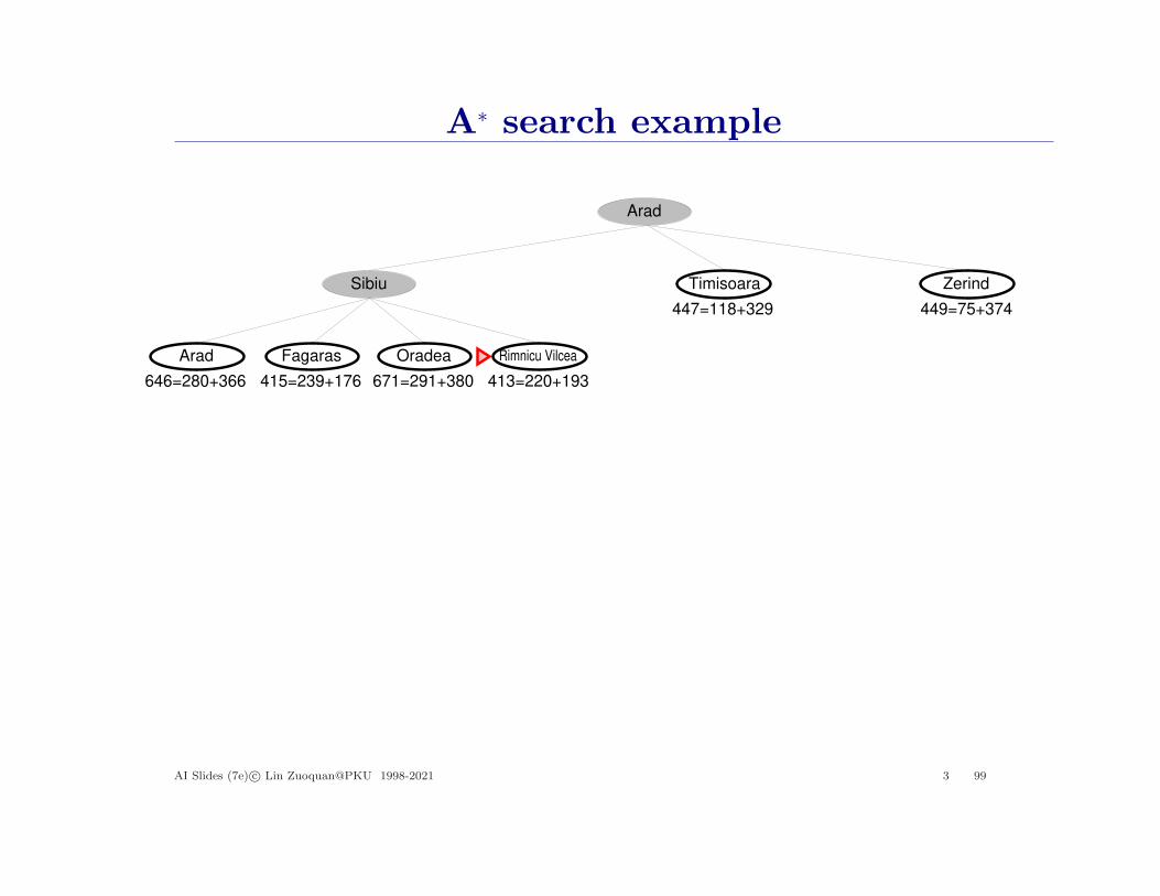
A∗ search example
Zerind
Arad
Sibiu
Arad
Timisoara
Rimnicu VilceaFagaras Oradea
447=118+329 449=75+374
646=280+366 413=220+193415=239+176 671=291+380
AI Slides (7e) c© Lin Zuoquan@PKU 1998-2021 3 99

A∗ search example
Zerind
Arad
Sibiu
Arad
Timisoara
Fagaras Oradea
447=118+329 449=75+374
646=280+366 415=239+176
Rimnicu Vilcea
Craiova Pitesti Sibiu
526=366+160 553=300+253417=317+100
671=291+380
AI Slides (7e) c© Lin Zuoquan@PKU 1998-2021 3 100

A∗ search example
Zerind
Arad
Sibiu
Arad
Timisoara
Sibiu Bucharest
Rimnicu VilceaFagaras Oradea
Craiova Pitesti Sibiu
447=118+329 449=75+374
646=280+366
591=338+253 450=450+0 526=366+160 553=300+253417=317+100
671=291+380
AI Slides (7e) c© Lin Zuoquan@PKU 1998-2021 3 101
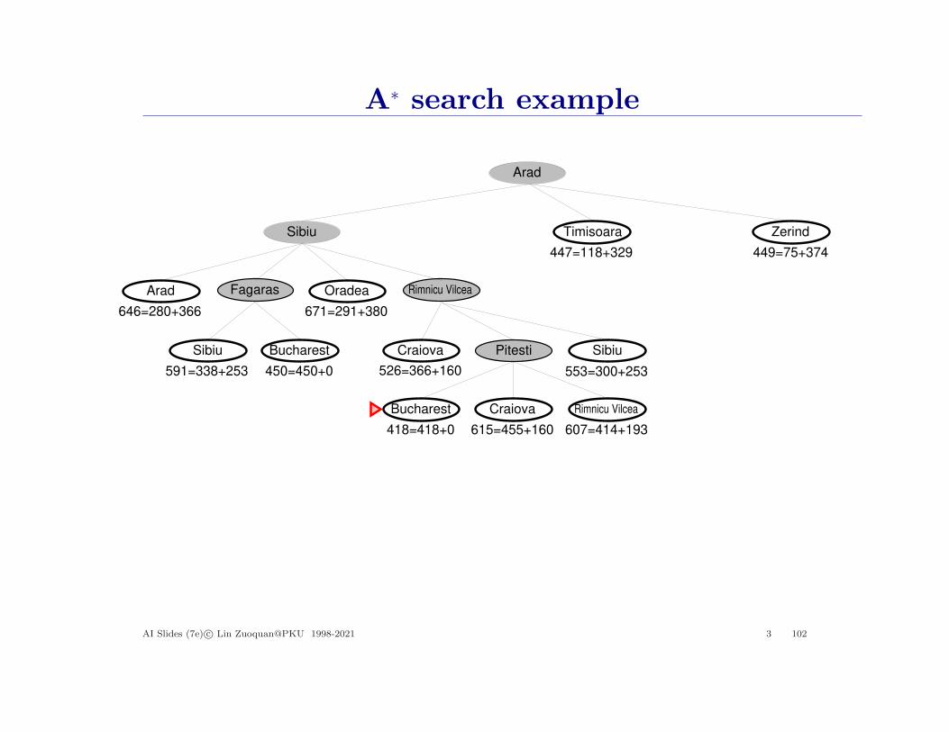
A∗ search example
Zerind
Arad
Sibiu
Arad
Timisoara
Sibiu Bucharest
Rimnicu VilceaFagaras Oradea
Craiova Pitesti Sibiu
Bucharest Craiova Rimnicu Vilcea
418=418+0
447=118+329 449=75+374
646=280+366
591=338+253 450=450+0 526=366+160 553=300+253
615=455+160 607=414+193
671=291+380
AI Slides (7e) c© Lin Zuoquan@PKU 1998-2021 3 102
Optimality of A∗
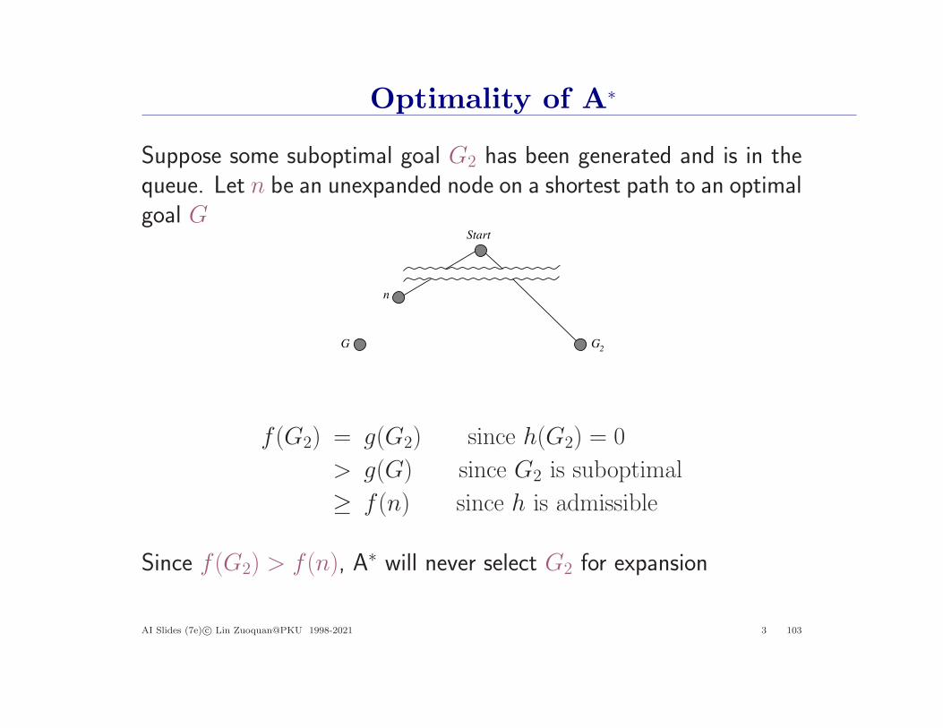
Suppose some suboptimal goal G2 has been generated and is in thequeue. Let n be an unexpanded node on a shortest path to an optimalgoal G
G
n
G2
Start
f (G2) = g(G2) since h(G2) = 0
> g(G) since G2 is suboptimal
≥ f (n) since h is admissible
Since f (G2) > f (n), A∗ will never select G2 for expansion
AI Slides (7e) c© Lin Zuoquan@PKU 1998-2021 3 103
Optimality of A∗
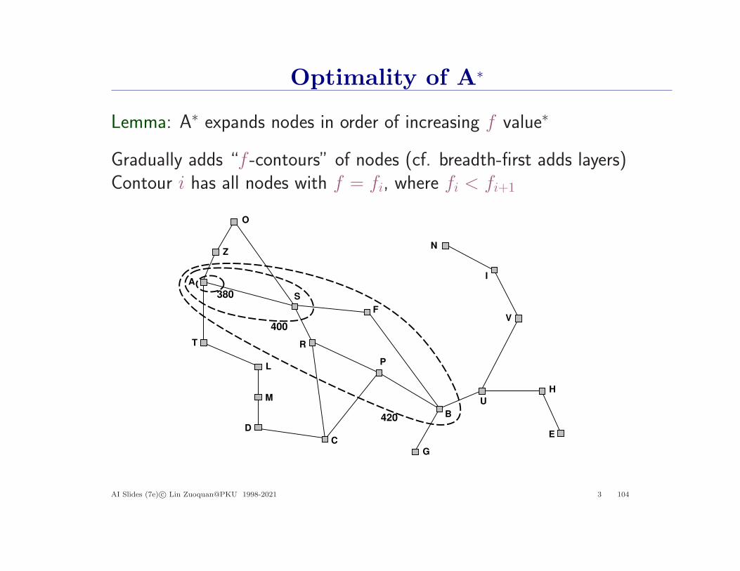
Lemma: A∗ expands nodes in order of increasing f value∗
Gradually adds “f -contours” of nodes (cf. breadth-first adds layers)Contour i has all nodes with f = fi, where fi < fi+1
O
Z
A
T
L
M
D
C
R
F
P
G
B
U
H
E
V
I
N
380
400
420
S
AI Slides (7e) c© Lin Zuoquan@PKU 1998-2021 3 104
Heuristic consistency
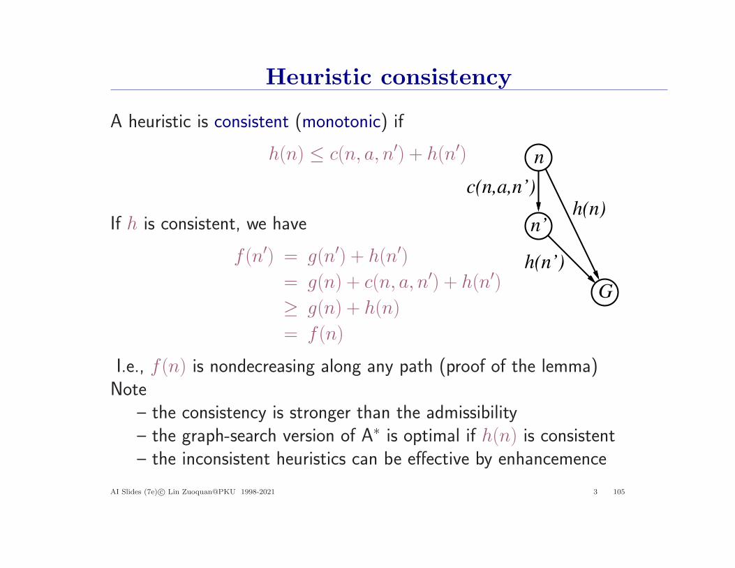
A heuristic is consistent (monotonic) if
n
c(n,a,n’)
h(n’)
h(n)
G
n’
h(n) ≤ c(n, a, n′) + h(n′)
If h is consistent, we have
f (n′) = g(n′) + h(n′)
= g(n) + c(n, a, n′) + h(n′)
≥ g(n) + h(n)
= f (n)
I.e., f (n) is nondecreasing along any path (proof of the lemma)Note
– the consistency is stronger than the admissibility– the graph-search version of A∗ is optimal if h(n) is consistent– the inconsistent heuristics can be effective by enhancemence
AI Slides (7e) c© Lin Zuoquan@PKU 1998-2021 3 105

Properties of A∗
Complete??
AI Slides (7e) c© Lin Zuoquan@PKU 1998-2021 3 106
Properties of A∗
Complete?? Yes, unless there are infinitely many nodes with f ≤f (G)
Time??
AI Slides (7e) c© Lin Zuoquan@PKU 1998-2021 3 107

Properties of A∗
Complete?? Yes, unless there are infinitely many nodes with f ≤f (G)
Time?? Exponential in [relative error in h × length of soln.]– absolute error: ∆ = h∗ − h, relative error: ǫ = (h∗ − h)/h∗
– exponential in the maximum absolute error, O(b∆)– for constant step costs, O(bǫd), or O((bǫ)d) w.r.t. h∗
(Polynomial in various variants of the heuristics)
Space??
AI Slides (7e) c© Lin Zuoquan@PKU 1998-2021 3 108
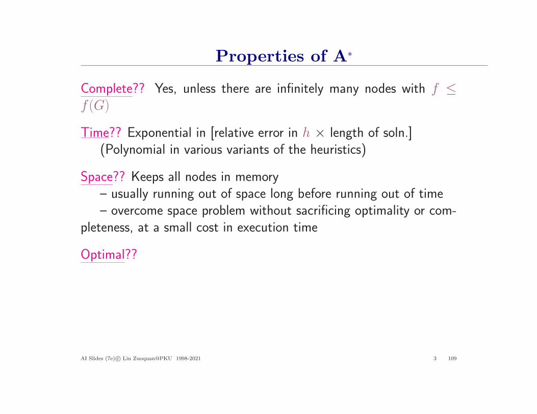
Properties of A∗
Complete?? Yes, unless there are infinitely many nodes with f ≤f (G)
Time?? Exponential in [relative error in h × length of soln.](Polynomial in various variants of the heuristics)
Space?? Keeps all nodes in memory– usually running out of space long before running out of time– overcome space problem without sacrificing optimality or com-
pleteness, at a small cost in execution time
Optimal??
AI Slides (7e) c© Lin Zuoquan@PKU 1998-2021 3 109

Properties of A∗
Complete?? Yes, unless there are infinitely many nodes with f ≤f (G)
Time?? Exponential in [relative error in h × length of soln.](Polynomial in various variants of the heuristics)
Space?? Keeps all nodes in memory
Optimal?? Yes — cannot expand fi+1 until fi is finished— optimally efficient
(C∗ is the cost of the optimal solution path)A∗ expands all nodes with f (n) < C∗
A∗ expands some nodes with f (n) = C∗
A∗ expands no nodes with f (n) > C∗
prune – eliminating possibilities without having to examine
AI Slides (7e) c© Lin Zuoquan@PKU 1998-2021 3 110
A∗ variants∗
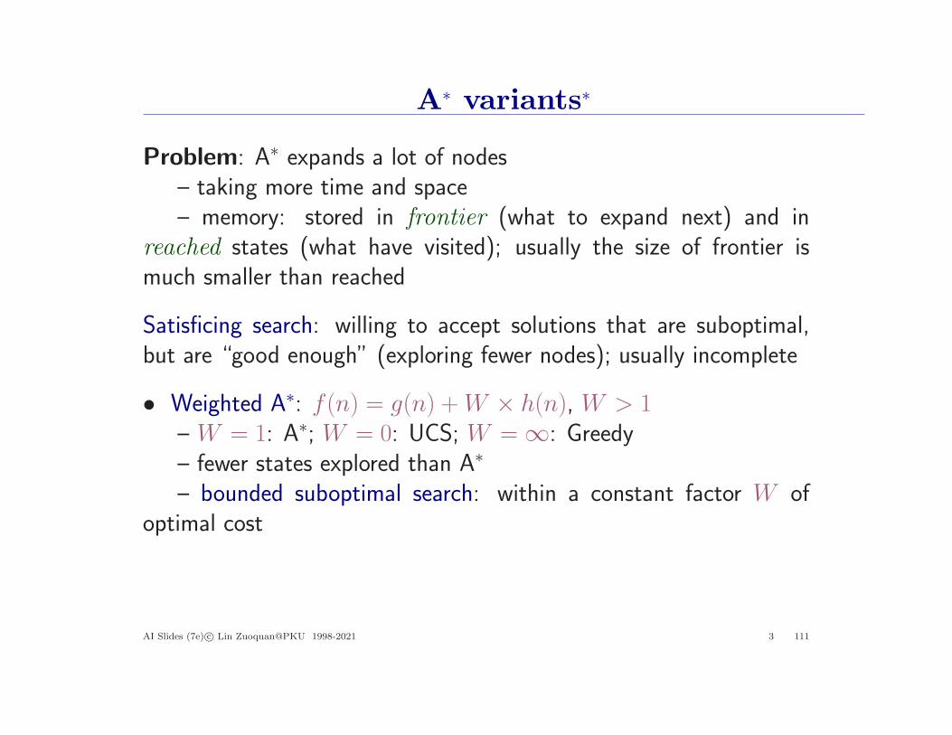
Problem: A∗ expands a lot of nodes– taking more time and space– memory: stored in frontier (what to expand next) and in
reached states (what have visited); usually the size of frontier ismuch smaller than reached
Satisficing search: willing to accept solutions that are suboptimal,but are “good enough” (exploring fewer nodes); usually incomplete
• Weighted A∗: f (n) = g(n) +W × h(n), W > 1– W = 1: A∗; W = 0: UCS; W =∞: Greedy– fewer states explored than A∗
– bounded suboptimal search: within a constant factor W ofoptimal cost
AI Slides (7e) c© Lin Zuoquan@PKU 1998-2021 3 111
A∗ variants∗
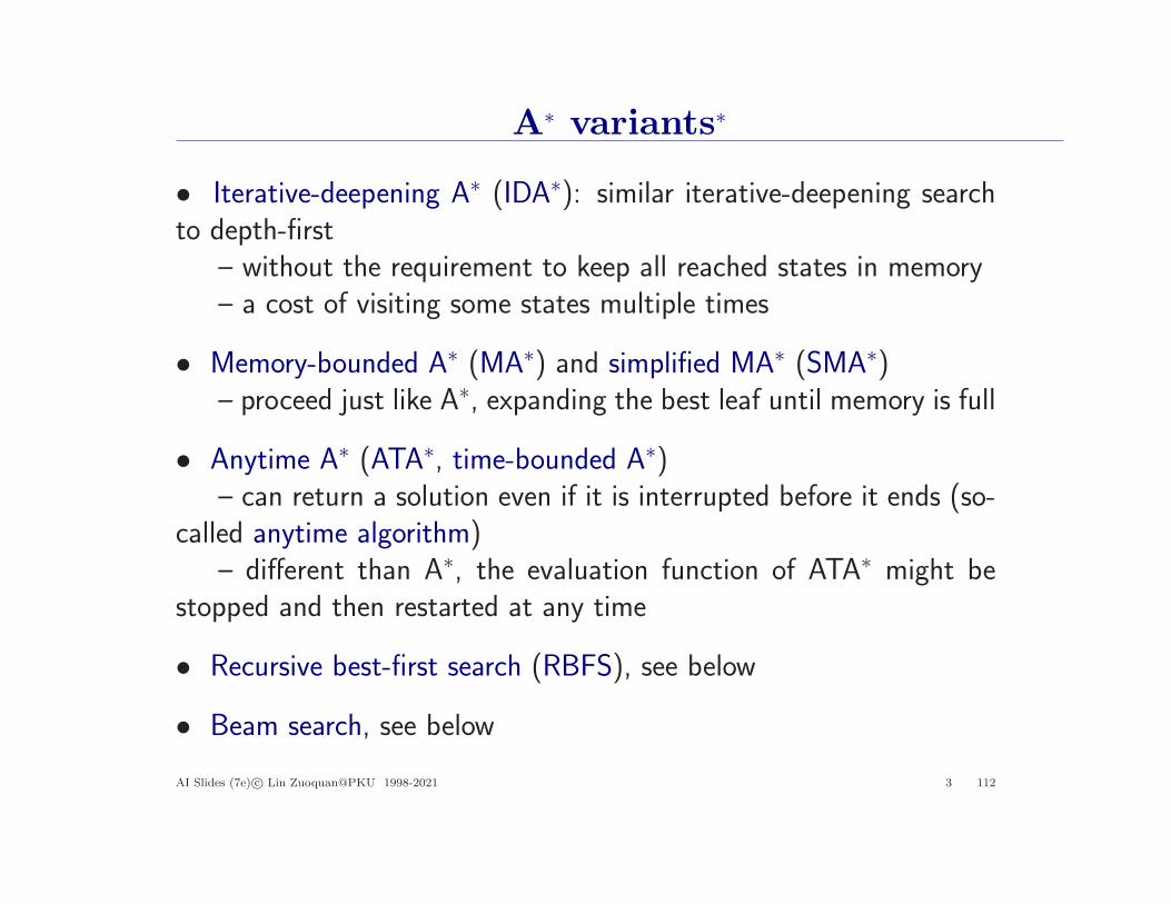
• Iterative-deepening A∗ (IDA∗): similar iterative-deepening searchto depth-first
– without the requirement to keep all reached states in memory– a cost of visiting some states multiple times
• Memory-bounded A∗ (MA∗) and simplified MA∗ (SMA∗)– proceed just like A∗, expanding the best leaf until memory is full
• Anytime A∗ (ATA∗, time-bounded A∗)– can return a solution even if it is interrupted before it ends (so-
called anytime algorithm)– different than A∗, the evaluation function of ATA∗ might be
stopped and then restarted at any time
• Recursive best-first search (RBFS), see below
• Beam search, see below
AI Slides (7e) c© Lin Zuoquan@PKU 1998-2021 3 112

Recursive best-first search
RBFS: recursive algorithm– best-first search, but using only linear space
– similar to recursive-DLS, but– – using the f-limit variable to keep track of the f -value of the
best alternative path available from any ancestor of the current node
Complete?? Yes, like to A∗
Time?? Exponential, depending both on the accuracy of f and onhow often the best path changes as nodes are expanded
Space?? linear in the depth of the deepest optimal solution
Optimal?? Yes, like to A∗ (if h(n) is admissible)
AI Slides (7e) c© Lin Zuoquan@PKU 1998-2021 3 113

Recursive best-first algorithm#
def Recursive-Best-First-Search( problem)
solution,fvalue←RBFS(problem,Note(problem.Initial),∞)
return solution
def RBFS(problem,node, f-limit)
if problem.Is-Goal(node.State) then return node
successors← LIST(Expand(node))
if successors is empty then return failure, ∞for each s in successors do // update f with value from previous search
s.f←max(s .Path-Cost + h(s), node.f )
while true do
best← the lowest f-value node in successors
if best.f > f-limit then return failure, best.f
alternative← the second-lowest f-value among successors
result, best.f←RBFS(problem, best,min(f-limit, alternative))
if result 6=failure then return result,best.f
AI Slides (7e) c© Lin Zuoquan@PKU 1998-2021 3 114
Beam search
Idea: keep k states instead of 1; choose top k of all their successors– keeping the k nodes with the best f-scores– limiting the size of the frontier, saving memory– incomplete and suboptimal
Not the same as k searches run in parallelSearches that find good states recruit other searches to join them
AI Slides (7e) c© Lin Zuoquan@PKU 1998-2021 3 115
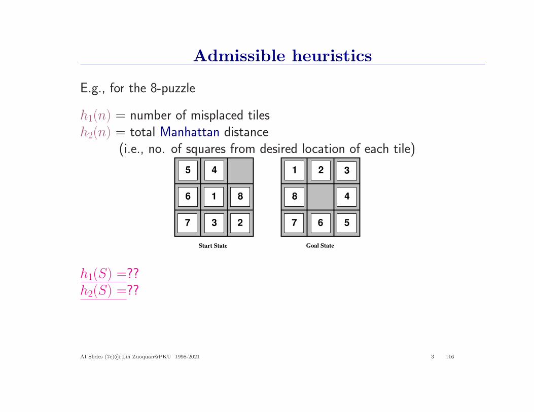
Admissible heuristics
E.g., for the 8-puzzle
h1(n) = number of misplaced tilesh2(n) = total Manhattan distance
(i.e., no. of squares from desired location of each tile)
Start State Goal State
2
45
6
7
8
1 2 3
4
67
81
23
45
6
7
81
23
45
6
7
8
5
h1(S) =??h2(S) =??
AI Slides (7e) c© Lin Zuoquan@PKU 1998-2021 3 116
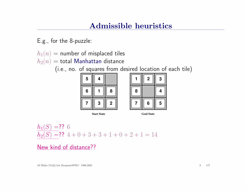
Admissible heuristics
E.g., for the 8-puzzle:
h1(n) = number of misplaced tilesh2(n) = total Manhattan distance
(i.e., no. of squares from desired location of each tile)
Start State Goal State
2
45
6
7
8
1 2 3
4
67
81
23
45
6
7
81
23
45
6
7
8
5
h1(S) =?? 6h2(S) =?? 4 + 0 + 3 + 3 + 1 + 0 + 2 + 1 = 14
New kind of distance??
AI Slides (7e) c© Lin Zuoquan@PKU 1998-2021 3 117

Dominance#
If h2(n) ≥ h1(n) for all n (both admissible)then h2 dominates h1 and is better for search
Typical search costs:
d = 14 IDS = 3,473,941 nodesA∗(h1) = 539 nodesA∗(h2) = 113 nodes
d = 24 IDS ≈ 54,000,000,000 nodesA∗(h1) = 39,135 nodesA∗(h2) = 1,641 nodes
Given any admissible heuristics ha, hb,
h(n) = max(ha(n), hb(n))
is also admissible and dominates ha, hb
AI Slides (7e) c© Lin Zuoquan@PKU 1998-2021 3 118

Relaxed problems#
Admissible heuristics can be derived from the exactsolution cost of a relaxed version of the problem
If the rules of the 8-puzzle are relaxed so that a tile can move any-where, then h1(n) gives the shortest solution
If the rules are relaxed so that a tile can move to any adjacent
square, then h2(n) gives the shortest solution
Key point: the optimal solution cost of a relaxed problemis no greater than the optimal solution cost of the real problem
AI Slides (7e) c© Lin Zuoquan@PKU 1998-2021 3 119
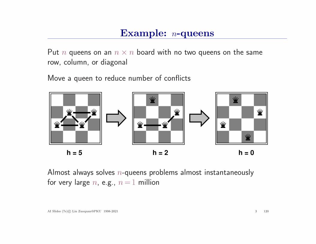
Example: n-queens
Put n queens on an n× n board with no two queens on the samerow, column, or diagonal
Move a queen to reduce number of conflicts
h = 5 h = 2 h = 0
Almost always solves n-queens problems almost instantaneouslyfor very large n, e.g., n=1 million
AI Slides (7e) c© Lin Zuoquan@PKU 1998-2021 3 120
Local Search
Local search algorithms operate using a single current (rather thanmultiple paths) and generally move only to neighbors of that node
Local search vs. global search– global search, including informed or uninformed search, system-
atically explore paths from an initial state– global search problems: observable, deterministic, known envi-
ronments– local search use very little memory and find reasonable solutions
in larger or infinite (continuous) state spaces for which global searchis unsuitable
AI Slides (7e) c© Lin Zuoquan@PKU 1998-2021 3 121
Local Search
Local search are useful for solving optimization problems
— the best estimate of “objective function”, e.g., reproductivefitness in nature by Darwinian evolution
Local search algorithms• Hill-climbing (greedy local search)• Simulated annealing• Genetic algorithms
AI Slides (7e) c© Lin Zuoquan@PKU 1998-2021 3 122
Hill-climbing
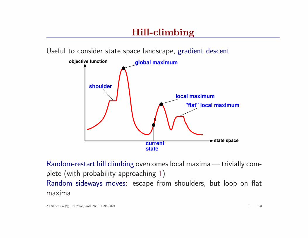
Useful to consider state space landscape, gradient descent
currentstate
objective function
state space
global maximum
local maximum
"flat" local maximum
shoulder
Random-restart hill climbing overcomes local maxima— trivially com-plete (with probability approaching 1)Random sideways moves: escape from shoulders, but loop on flatmaxima
AI Slides (7e) c© Lin Zuoquan@PKU 1998-2021 3 123
Hill-climbing
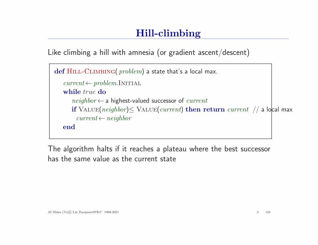
Like climbing a hill with amnesia (or gradient ascent/descent)
def Hill-Climbing( problem) a state that’s a local max.
current← problem.Initial
while true do
neighbor← a highest-valued successor of current
if Value(neighbor)≤ Value(current) then return current // a local max
current← neighbor
end
The algorithm halts if it reaches a plateau where the best successorhas the same value as the current state
AI Slides (7e) c© Lin Zuoquan@PKU 1998-2021 3 124
Simulated annealing∗
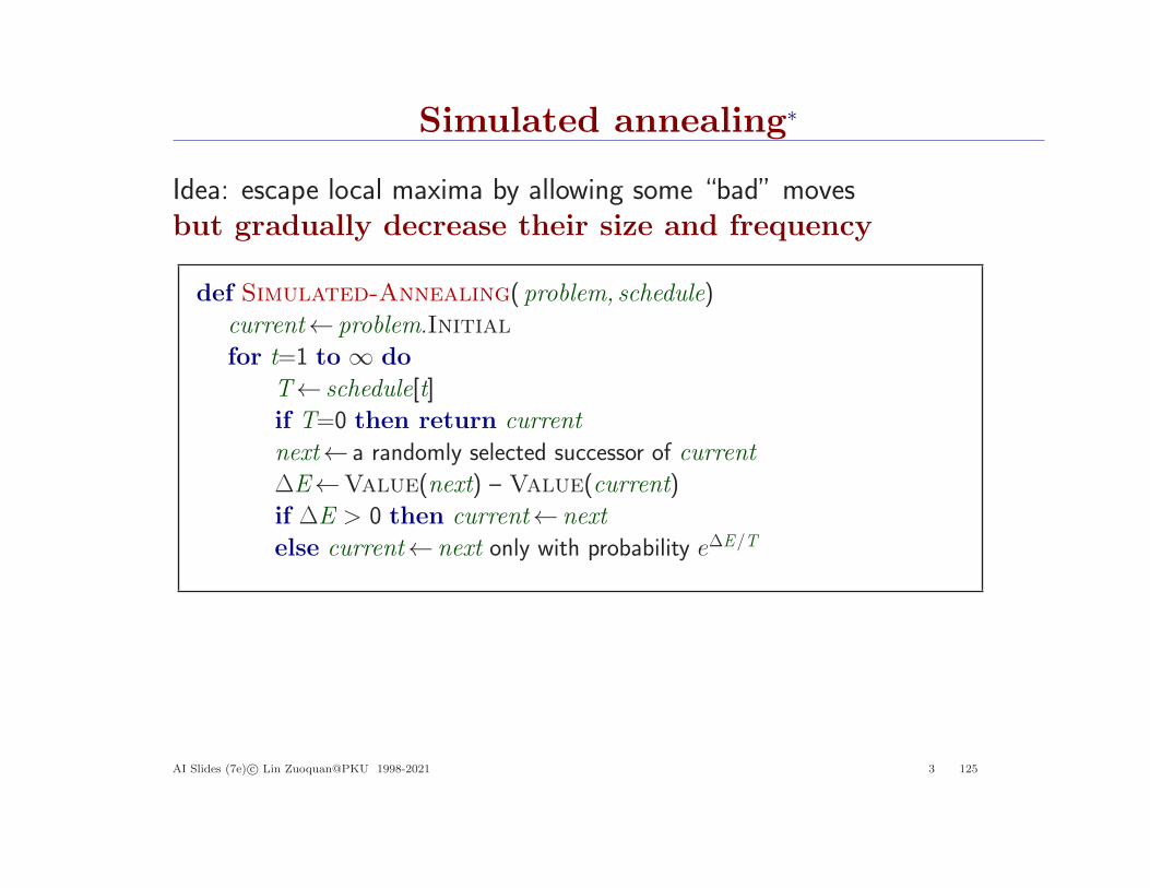
Idea: escape local maxima by allowing some “bad” movesbut gradually decrease their size and frequency
def Simulated-Annealing( problem, schedule)
current← problem.Initial
for t=1 to ∞ do
T← schedule[t]
if T=0 then return current
next← a randomly selected successor of current
∆E←Value(next) – Value(current)
if ∆E > 0 then current← next
else current← next only with probability e∆E/T
AI Slides (7e) c© Lin Zuoquan@PKU 1998-2021 3 125

Properties of simulated annealing
At fixed “temperature” T , state occupation probability reachesBoltzman distribution (see later in probabilistic distribuiton)
p(x) = αeE(x)kT
T decreased slowly enough =⇒ always reach best state x∗
because eE(x∗)kT /e
E(x)kT = e
E(x∗)−E(x)kT ≫ 1 for small T
find a global optimum with probability approaching 1
Devised (Metropolis et al., 1953) for physical process modeling
Simulated annealing is a field in itself, widely used in VLSI layout,airline scheduling, etc.
AI Slides (7e) c© Lin Zuoquan@PKU 1998-2021 3 126
Local beam search
Beam search by local search to choose top k of all their successors
Problem: quite often, all k states end up on same local hill
Idea: choose k successors randomly (stochastic beam search), biasedtowards good ones
Observe the close analogy to natural selection
AI Slides (7e) c© Lin Zuoquan@PKU 1998-2021 3 127

Genetic algorithms∗
GA= stochastic local beam search + generate successors from pairs
of states
32252124
Selection Cross−Over Mutation
24748552
32752411
24415124
24
23
20
32543213 11
29%
31%
26%
14%
32752411
24748552
32752411
24415124
32748552
24752411
32752124
24415411
24752411
32748152
24415417
Fitness Pairs
AI Slides (7e) c© Lin Zuoquan@PKU 1998-2021 3 128

Genetic algorithms
GAs require states encoded as strings (GPs use programs)
Crossover helps iff substrings are meaningful components
+ =
GAs 6= evolution: e.g., real genes encode replication machinery
A.k.a, evolutionary algorithms
Genetic programming (GP) is closely related to GAs
Artificial Life (AL) moves one step further
AI Slides (7e) c© Lin Zuoquan@PKU 1998-2021 3 129

Local search in continuous state spaces∗
Suppose we want to site three airports in Romania– 6-D state space defined by (x1, y2), (x2, y2), (x3, y3)– objective function f (x1, y2, x2, y2, x3, y3) =
sum of squared distances from each city to nearest airportDiscretization methods turn continuous space into discrete space,e.g., empirical gradient considers ±δ change in each coordinateGradient methods compute
∇f =
∂f
∂x1,∂f
∂y1,∂f
∂x2,∂f
∂y2,∂f
∂x3,∂f
∂y3
to increase/reduce f , e.g., by x← x + α∇f (x)Sometimes can solve for ∇f (x) = 0 exactly (e.g., with one city).Newton–Raphson (1664, 1690) iterates x← x−H−1f (x)∇f (x)to solve ∇f (x) = 0, where Hij = ∂2f/∂xi∂xj
Hint: Newton-Raphson method is an efficient local search
AI Slides (7e) c© Lin Zuoquan@PKU 1998-2021 3 130
Online search∗
Offline search algorithms compute a complete solution before exec.vs.
online search ones interleave computation and action (processing in-put data as they are received)
– necessary for unknown environment(dynamic or semidynamic, and nonderterministic domains)⇐ exploration problem
AI Slides (7e) c© Lin Zuoquan@PKU 1998-2021 3 131
Example: maze problem
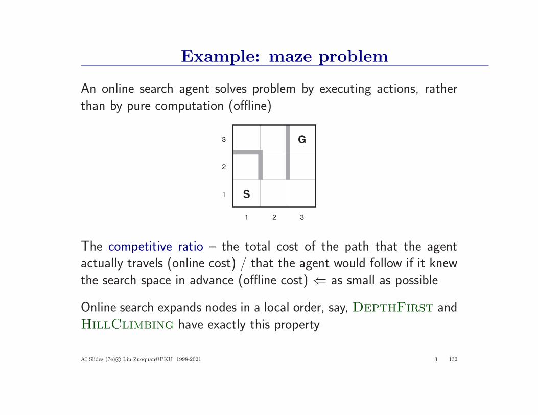
An online search agent solves problem by executing actions, ratherthan by pure computation (offline)
G
S1
2
3
1 2 3
The competitive ratio – the total cost of the path that the agentactually travels (online cost) / that the agent would follow if it knewthe search space in advance (offline cost) ⇐ as small as possible
Online search expands nodes in a local order, say, DepthFirst andHillClimbing have exactly this property
AI Slides (7e) c© Lin Zuoquan@PKU 1998-2021 3 132
Online search agents#
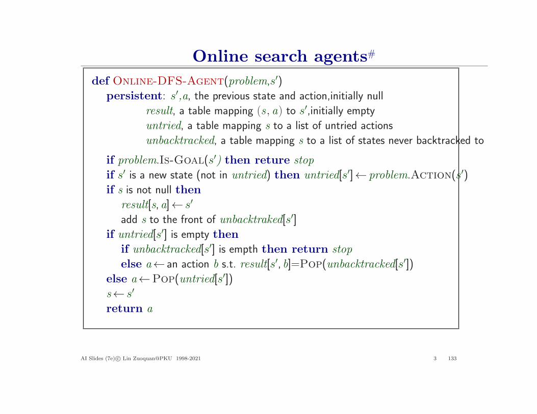
def Online-DFS-Agent(problem,s′)persistent: s′,a, the previous state and action,initially null
result, a table mapping (s , a) to s′,initially emptyuntried, a table mapping s to a list of untried actions
unbacktracked, a table mapping s to a list of states never backtracked to
if problem.Is-Goal(s′) then reture stop
if s′ is a new state (not in untried) then untried[s′]← problem.Action(s′)if s is not null then
result[s,a]← s′
add s to the front of unbacktraked[s′]if untried[s′] is empty then
if unbacktracked[s′] is empth then return stop
else a← an action b s.t. result[s′, b]=Pop(unbacktracked[s′])else a←Pop(untried[s′])s← s′
return a
AI Slides (7e) c© Lin Zuoquan@PKU 1998-2021 3 133
Adversarial search
• Games
• Perfect play– minimax decisions– α–β pruning
• Imperfect play– Monte Carlo tree search
AI Slides (7e) c© Lin Zuoquan@PKU 1998-2021 3 134
Games
Game as adversarial search
“Unpredictable” opponent ⇒ solution is a strategyspecifying a move for every possible opponent reply
Time limits ⇒ unlikely to find goal, must approximatePlan of attack
• Computer considers possible lines of play (Babbage, 1846)• Algorithm for perfect play (Zermelo, 1912; Von Neumann, 1944)
• Finite horizon, approximate evaluation (Zuse, 1945; Wiener, 1948;Shannon, 1950)
• First chess program (Turing, 1951)
•Machine learning to improve evaluation accuracy (Samuel, 1952–57)
• Pruning to allow deeper search (McCarthy, 1956)
AI Slides (7e) c© Lin Zuoquan@PKU 1998-2021 3 135
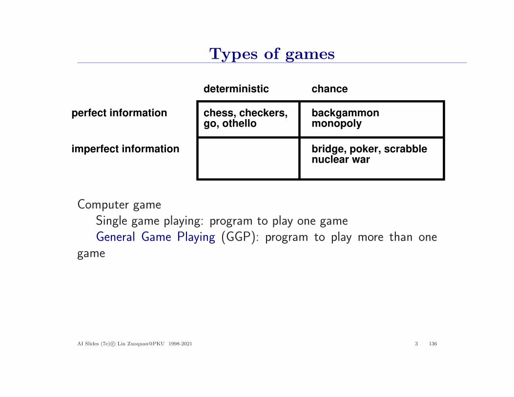
Types of games
deterministic chance
perfect information
imperfect information
chess, checkers,go, othello
backgammonmonopoly
bridge, poker, scrabblenuclear war
Computer gameSingle game playing: program to play one gameGeneral Game Playing (GGP): program to play more than one
game
AI Slides (7e) c© Lin Zuoquan@PKU 1998-2021 3 136
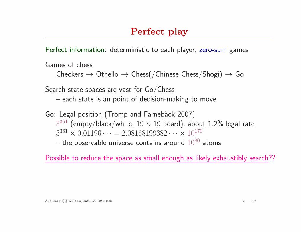
Perfect play
Perfect information: deterministic to each player, zero-sum games
Games of chessCheckers → Othello → Chess(/Chinese Chess/Shogi) → Go
Search state spaces are vast for Go/Chess– each state is an point of decision-making to move
Go: Legal position (Tromp and Farneback 2007)3361 (empty/black/white, 19× 19 board), about 1.2% legal rate3361 × 0.01196 · · · = 2.08168199382 · · · × 10170
– the observable universe contains around 1080 atoms
Possible to reduce the space as small enough as likely exhaustibly search??
AI Slides (7e) c© Lin Zuoquan@PKU 1998-2021 3 137
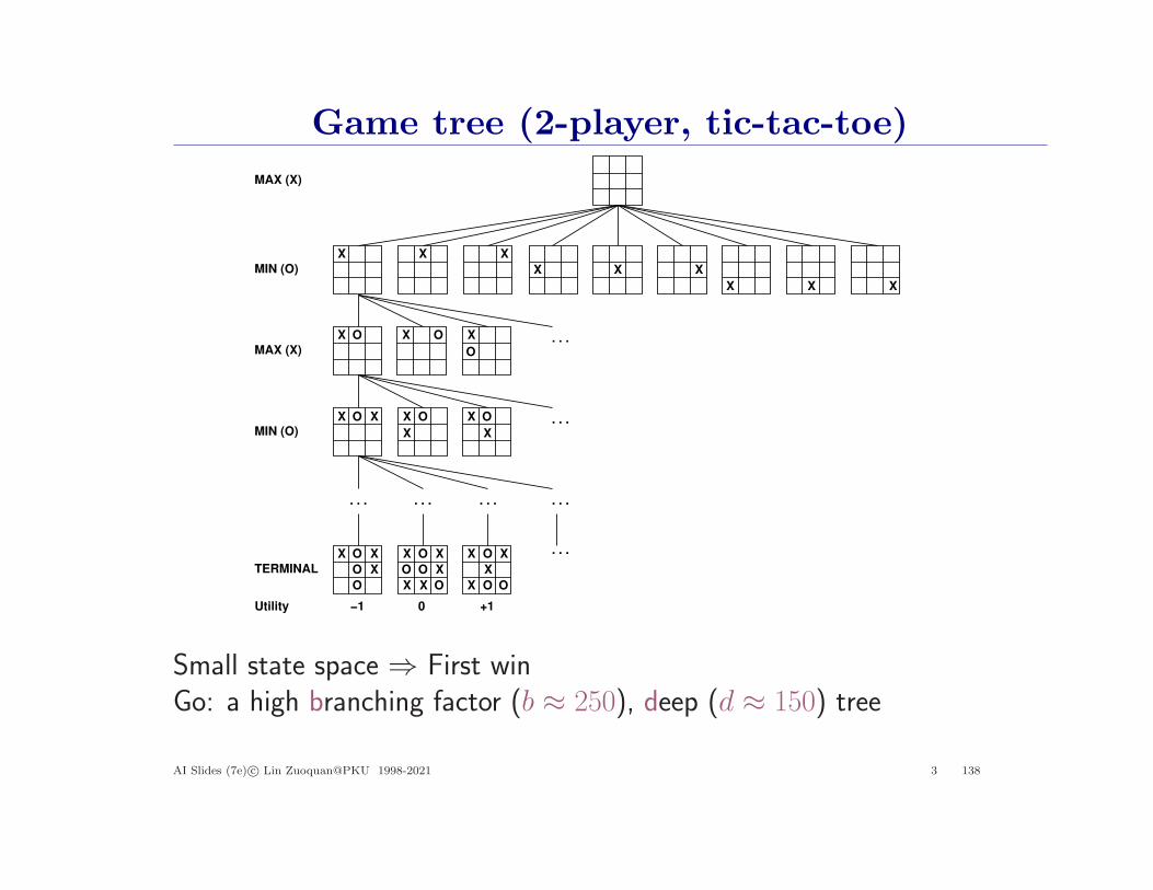
Game tree (2-player, tic-tac-toe)
XX
XX
X
X
X
XX
MAX (X)
MIN (O)
X X
O
O
OX O
O
O O
O OO
MAX (X)
X OX OX O X
X X
X
X
X X
MIN (O)
X O X X O X X O X
. . . . . . . . . . . .
. . .
. . .
. . .
TERMINAL
XX
−1 0 +1Utility
Small state space ⇒ First winGo: a high branching factor (b ≈ 250), deep (d ≈ 150) tree
AI Slides (7e) c© Lin Zuoquan@PKU 1998-2021 3 138
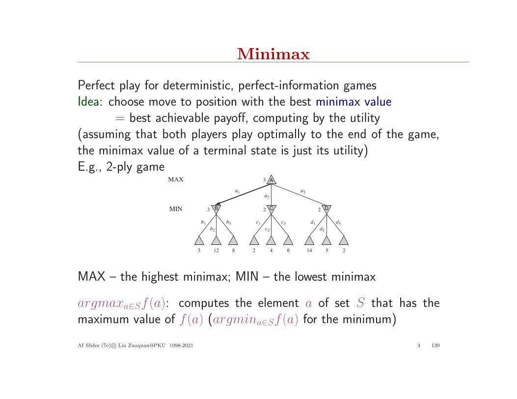
Minimax
Perfect play for deterministic, perfect-information gamesIdea: choose move to position with the best minimax value
= best achievable payoff, computing by the utility(assuming that both players play optimally to the end of the game,the minimax value of a terminal state is just its utility)E.g., 2-ply game
MAX A
B C D
3 12 8 2 4 6 14 5 2
3 2 2
3
a1
a2
a3
b1
b2
b3 c1
c2
c3 d1
d2
d3
MIN
MAX – the highest minimax; MIN – the lowest minimax
argmaxa∈Sf (a): computes the element a of set S that has themaximum value of f (a) (argmina∈Sf (a) for the minimum)
AI Slides (7e) c© Lin Zuoquan@PKU 1998-2021 3 139

Minimax algorithm
def Minimax-Search(game,state)
player← game.To-Move(state) //The player’s turn is to move
value,move←Max-Value(game,state)
return move //an action
def Max-Value(game,state)
if game.Is-Terminal(state) then return game.Utility(state,palyer),null
// a utility function defines the final numeric value to player
v←−∞for each a in game.Actions(state) do
v2,a2←Min-Value(game,game.Result(state,a))
if v2 > v then
v,move← v2,a
return v,move //a (utility,move) pair
AI Slides (7e) c© Lin Zuoquan@PKU 1998-2021 3 140
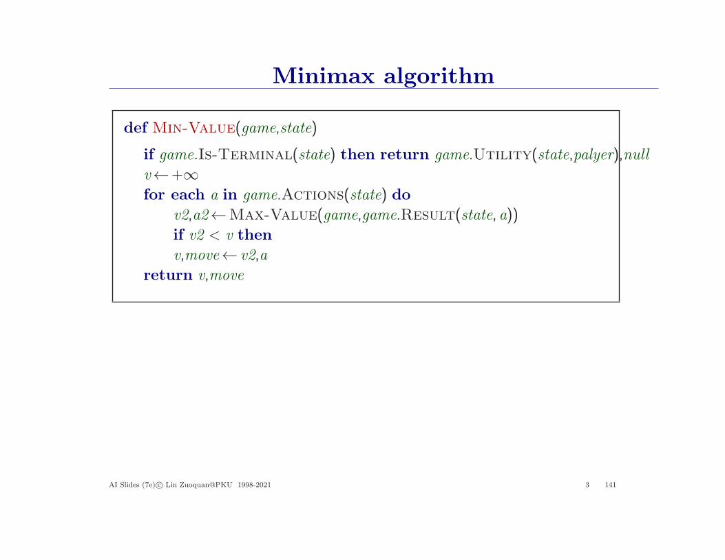
Minimax algorithm
def Min-Value(game,state)
if game.Is-Terminal(state) then return game.Utility(state,palyer),null
v←+∞for each a in game.Actions(state) do
v2,a2←Max-Value(game,game.Result(state,a))
if v2 < v then
v,move← v2,a
return v,move
AI Slides (7e) c© Lin Zuoquan@PKU 1998-2021 3 141

Properties of minimax#
Complete??
AI Slides (7e) c© Lin Zuoquan@PKU 1998-2021 3 142

Properties of minimax
Complete?? Only if tree is finite (chess has specific rules for this)(A finite strategy can exist even in an infinite tree)
Optimal??
AI Slides (7e) c© Lin Zuoquan@PKU 1998-2021 3 143
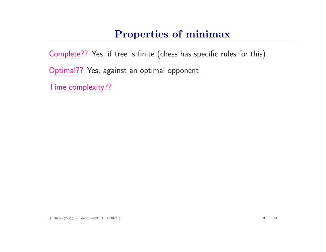
Properties of minimax
Complete?? Yes, if tree is finite (chess has specific rules for this)
Optimal?? Yes, against an optimal opponent
Time complexity??
AI Slides (7e) c© Lin Zuoquan@PKU 1998-2021 3 144

Properties of minimax
Complete?? Yes, if tree is finite (chess has specific rules for this)
Optimal?? Yes, against an optimal opponent. Otherwise??
Time complexity?? O(bm)
Space complexity??
AI Slides (7e) c© Lin Zuoquan@PKU 1998-2021 3 145
Properties of minimax
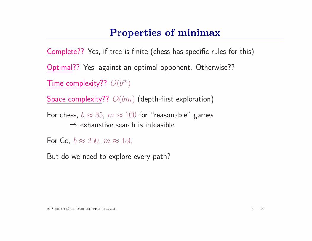
Complete?? Yes, if tree is finite (chess has specific rules for this)
Optimal?? Yes, against an optimal opponent. Otherwise??
Time complexity?? O(bm)
Space complexity?? O(bm) (depth-first exploration)
For chess, b ≈ 35, m ≈ 100 for “reasonable” games⇒ exhaustive search is infeasible
For Go, b ≈ 250, m ≈ 150
But do we need to explore every path?
AI Slides (7e) c© Lin Zuoquan@PKU 1998-2021 3 146
α–β pruning
..
..
..
MAX
MIN
MAX
MIN V
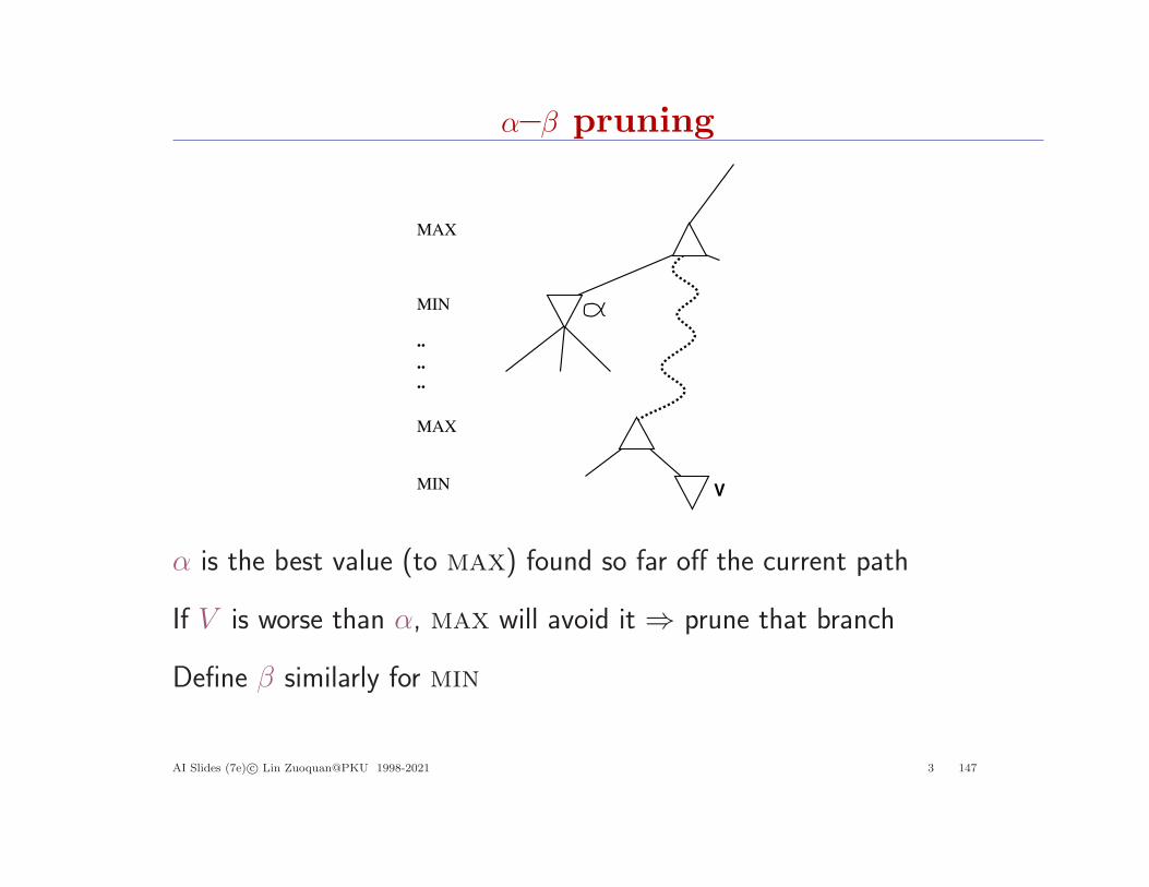
α is the best value (to max) found so far off the current path
If V is worse than α, max will avoid it ⇒ prune that branch
Define β similarly for min
AI Slides (7e) c© Lin Zuoquan@PKU 1998-2021 3 147
Example: α–β pruning
MAX
3 12 8
MIN 3
3
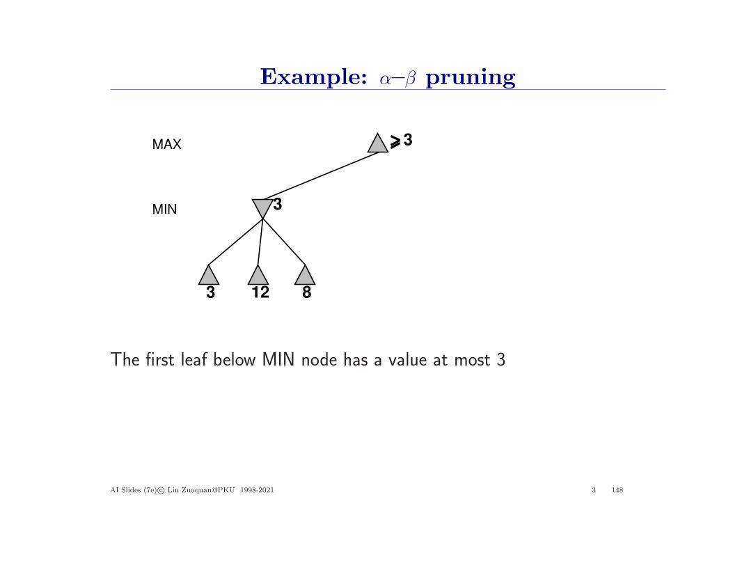
The first leaf below MIN node has a value at most 3
AI Slides (7e) c© Lin Zuoquan@PKU 1998-2021 3 148
Example: α–β pruning
MAX
3 12 8
MIN 3
2
2
X X
3
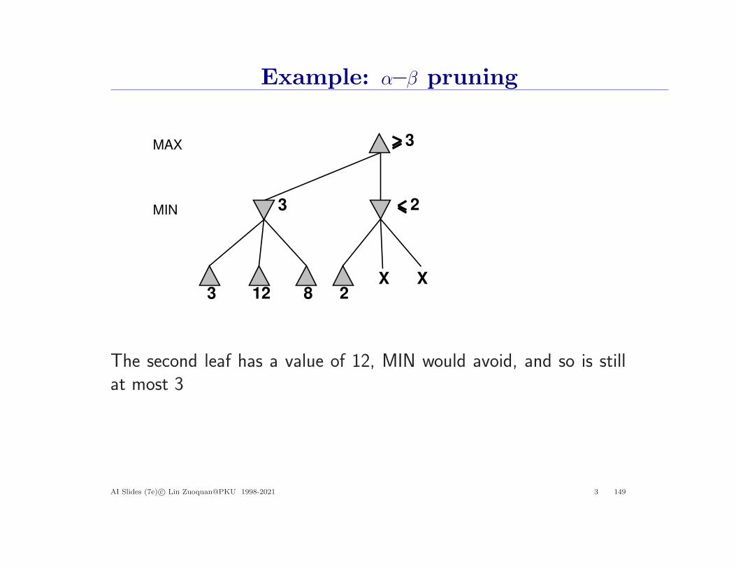
The second leaf has a value of 12, MIN would avoid, and so is stillat most 3
AI Slides (7e) c© Lin Zuoquan@PKU 1998-2021 3 149
Example: α–β pruning
MAX
3 12 8
MIN 3
2
2
X X14
14
3
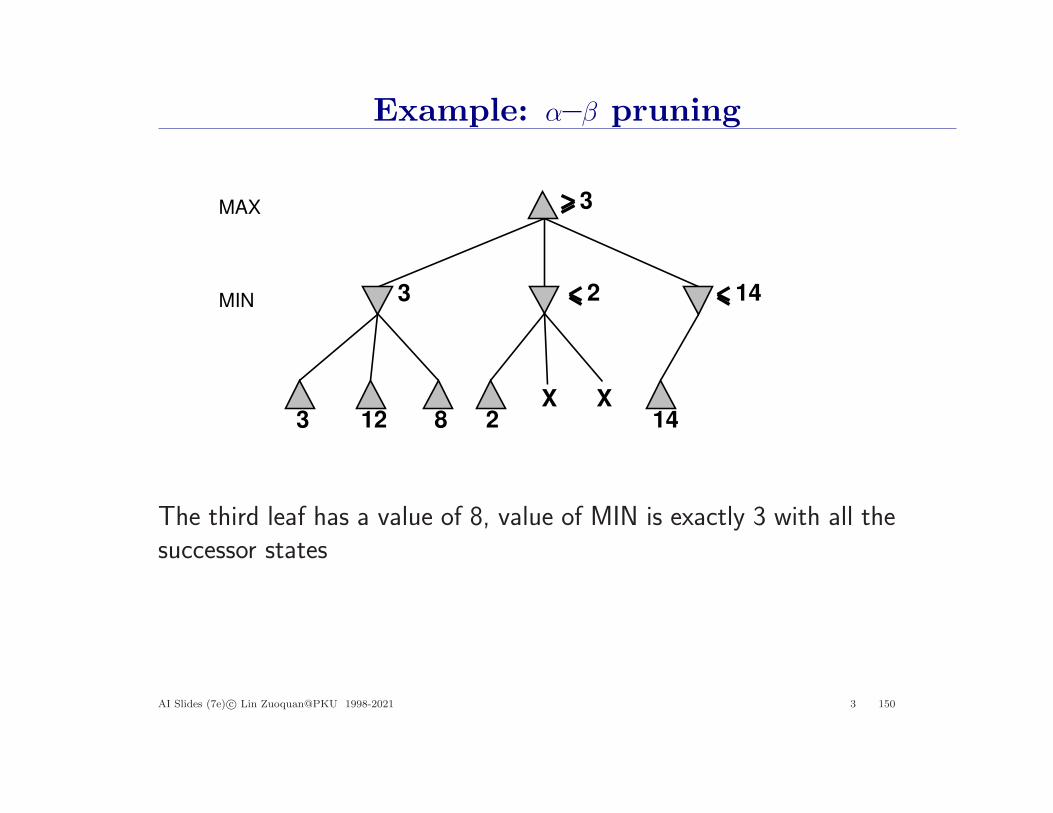
The third leaf has a value of 8, value of MIN is exactly 3 with all thesuccessor states
AI Slides (7e) c© Lin Zuoquan@PKU 1998-2021 3 150
Example: α–β pruning
MAX
3 12 8
MIN 3
2
2
X X14
14
5
5
3
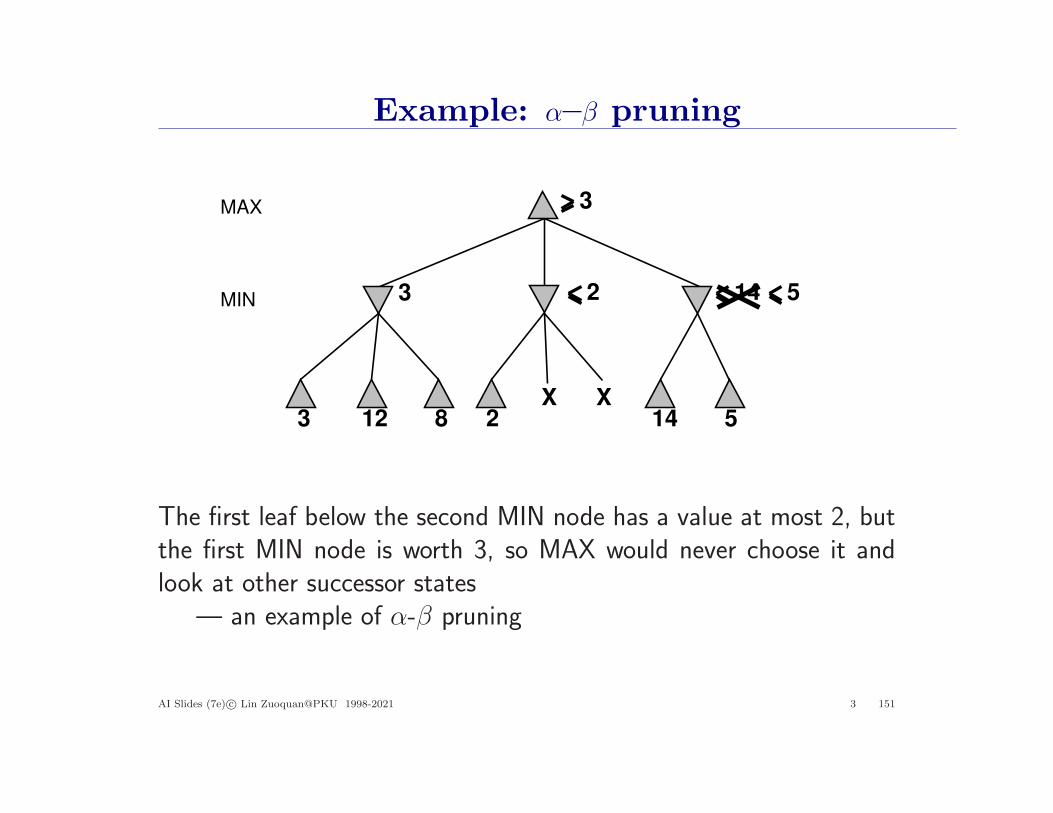
The first leaf below the second MIN node has a value at most 2, butthe first MIN node is worth 3, so MAX would never choose it andlook at other successor states
— an example of α-β pruning
AI Slides (7e) c© Lin Zuoquan@PKU 1998-2021 3 151
Example: α–β pruning
MAX
3 12 8
MIN
3
3
2
2
X X14
14
5
5
2
2
3
AI Slides (7e) c© Lin Zuoquan@PKU 1998-2021 3 152

The α–β algorithm
def Alpha-Beta-Pruning(game,state)
player← game.To-Move(state)
value,move←Max-Value(game,state,−∞,+∞)
return value
def Max-Value(game,state,α,β)
if game.Is-Terminal(state) then return game.Utility(state,palyer),null
v←−∞for each a in game.Actions(state) do
v2,a2←Min-Value(game,game.Result(state,a),α,β)
if v2 > v then
v,move← v2,a
α←Max(α,v)
if v ≥ β then return v,move
return v,move
AI Slides (7e) c© Lin Zuoquan@PKU 1998-2021 3 153

The α–β algorithm
def Min-Value(game,state,α,β)
if game.Is-Terminal(state) then return game.Utility(state,palyer),null
v←−∞for each a in game.Actions(state) do
v2,a2←Max-Value(game,game.Result(state,a),α,β)
if v2 < v then
v,move← v2,a
α←Max(α,v)
if v ≤ α then return v,move
return v,move
AI Slides (7e) c© Lin Zuoquan@PKU 1998-2021 3 154
Properties of α–β
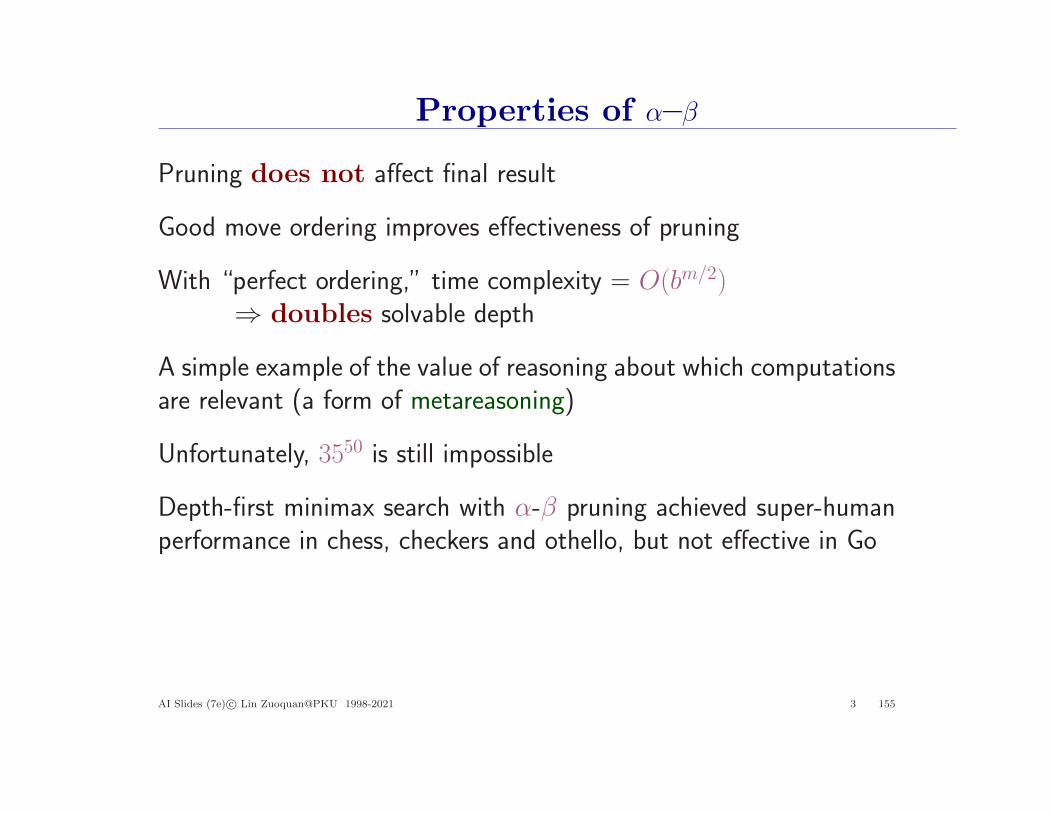
Pruning does not affect final result
Good move ordering improves effectiveness of pruning
With “perfect ordering,” time complexity = O(bm/2)⇒ doubles solvable depth
A simple example of the value of reasoning about which computationsare relevant (a form of metareasoning)
Unfortunately, 3550 is still impossible
Depth-first minimax search with α-β pruning achieved super-humanperformance in chess, checkers and othello, but not effective in Go
AI Slides (7e) c© Lin Zuoquan@PKU 1998-2021 3 155
Imperfect play
Resource limits– deterministic game may have imperfect information in real time
• Use Cutoff-Test instead of Is-Terminale.g., depth limit
• Use Eval instead of Utilityi.e., eval. function that estimates desirability of position
Suppose we have 100 seconds, explore 104 nodes/second⇒ 106 nodes per move ≈ 358/2
⇒ α–β reaches depth 8 ⇒ pretty good chess program
AI Slides (7e) c© Lin Zuoquan@PKU 1998-2021 3 156

Evaluation functions
Black to move
White slightly better
White to move
Black winning
For chess, typically linear weighted sum of features
Eval(s) = w1f1(s) + w2f2(s) + . . . + wnfn(s)
e.g., w1 = 9 withf1(s) = (number of white queens) – (number of black queens), etc.
AI Slides (7e) c© Lin Zuoquan@PKU 1998-2021 3 157
Evaluation functions
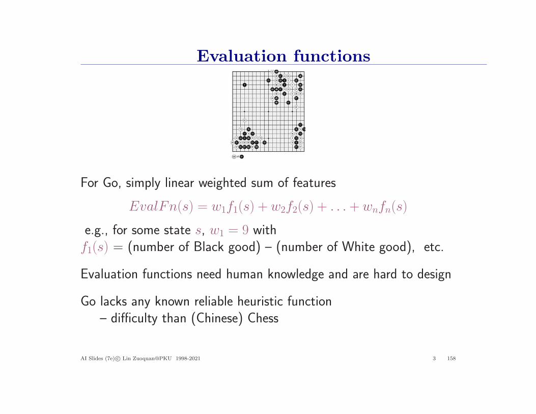
For Go, simply linear weighted sum of features
EvalFn(s) = w1f1(s) + w2f2(s) + . . . + wnfn(s)
e.g., for some state s, w1 = 9 withf1(s) = (number of Black good) – (number of White good), etc.
Evaluation functions need human knowledge and are hard to design
Go lacks any known reliable heuristic function– difficulty than (Chinese) Chess
AI Slides (7e) c© Lin Zuoquan@PKU 1998-2021 3 158
Deterministic (perfect information) games in practice
Checkers: Chinook ended 40-year-reign of human world championMarion Tinsley in 1994. Used an endgame database defining perfectplay for all positions involving 8 or fewer pieces on the board, a totalof 443,748,401,247 positions
Othello: human champions refuse to compete against computers,who are too good
Chess: IBM Deep Blue defeated human world champion Gary Kas-parov in 1997. Deep Blue uses very sophisticated evaluation, andundisclosed methods for extending some lines of search up to 40 ply
AI Slides (7e) c© Lin Zuoquan@PKU 1998-2021 3 159
Deterministic games in practice
Go: Google Deep MindAlphaGo
– Defeated human world champion Lee Sedol in 2016 and Ke Jiein 2017
– AlphaGo Zero defeated the champion-defeating versions Al-phaGo Lee/Master in 2017
– AlphaZero: a GGP program, achieved within 24h a superhumanlevel of play in the games of Chess/Shogi/Go (defeated AlphaGoZero) in Dec. 2017
MuZero: extension of AlphaZero including Atari in 2019– outperform AlphaZero– without any knowledge of the game rules
Achievements:• “the God of the chess” of superhuman• self-learning without prior human knowledge
AI Slides (7e) c© Lin Zuoquan@PKU 1998-2021 3 160
Deterministic games in practice
Chinese Chess: there is not seriously studied yet– in principle, the algorithm of AlphaZero can be directly used
for Chess and similar deterministic games
All deterministic games have being well defeated by AI
AI Slides (7e) c© Lin Zuoquan@PKU 1998-2021 3 161
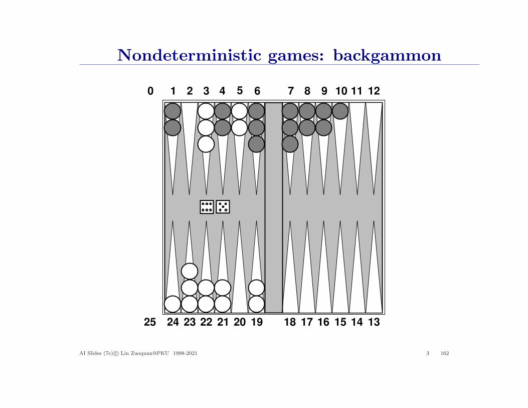
Nondeterministic games: backgammon
1 2 3 4 5 6 7 8 9 10 11 12
24 23 22 21 20 19 18 17 16 15 14 13
0
25
AI Slides (7e) c© Lin Zuoquan@PKU 1998-2021 3 162
Nondeterministic games in general
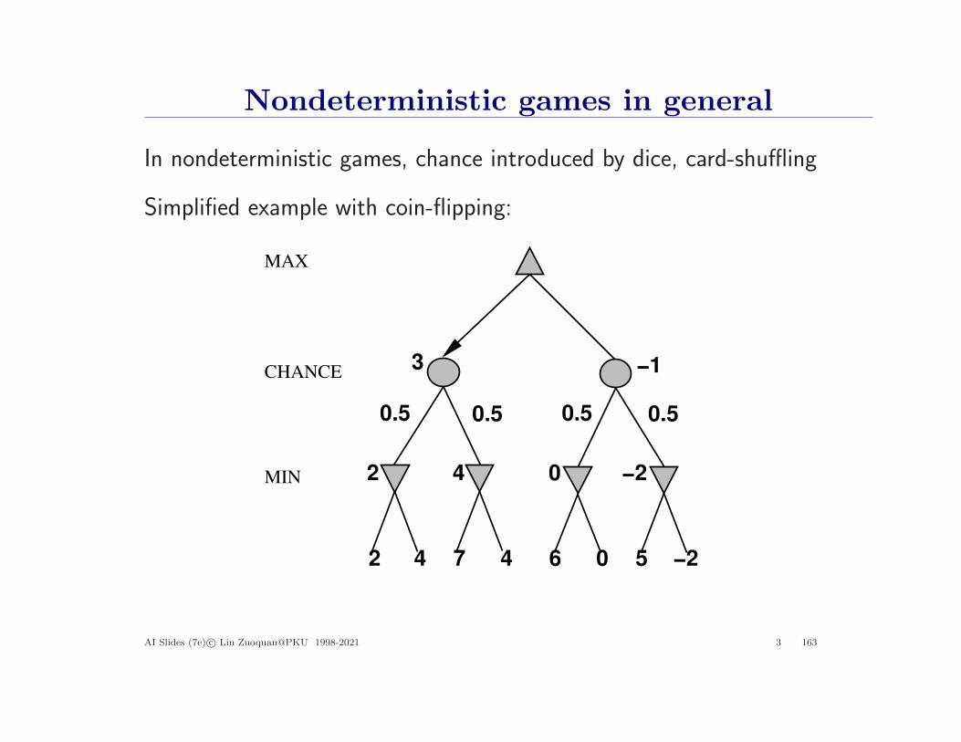
In nondeterministic games, chance introduced by dice, card-shuffling
Simplified example with coin-flipping:
MIN
MAX
2
CHANCE
4 7 4 6 0 5 −2
2 4 0 −2
0.5 0.5 0.5 0.5
3 −1
AI Slides (7e) c© Lin Zuoquan@PKU 1998-2021 3 163
Algorithm for nondeterministic games
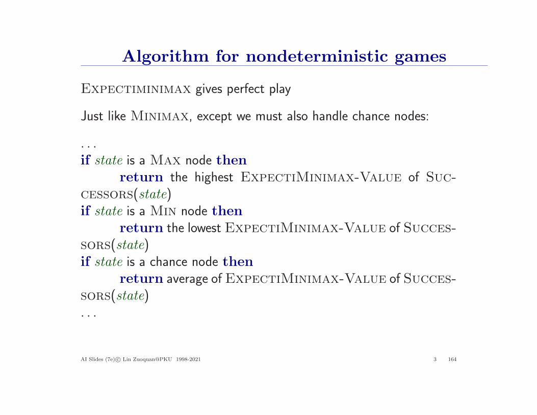
Expectiminimax gives perfect play
Just like Minimax, except we must also handle chance nodes:
. . .if state is a Max node then
return the highest ExpectiMinimax-Value of Suc-cessors(state)if state is a Min node then
return the lowest ExpectiMinimax-Value of Succes-sors(state)if state is a chance node then
return average of ExpectiMinimax-Value of Succes-sors(state). . .
AI Slides (7e) c© Lin Zuoquan@PKU 1998-2021 3 164
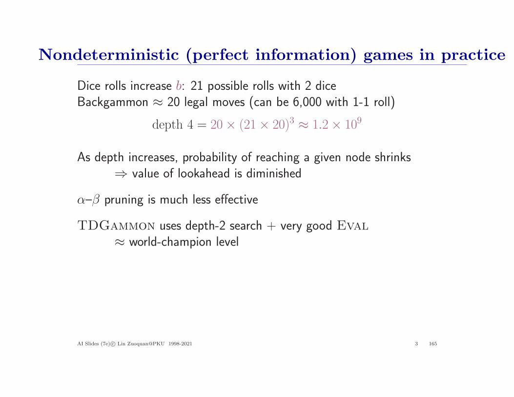
Nondeterministic (perfect information) games in practice
Dice rolls increase b: 21 possible rolls with 2 diceBackgammon ≈ 20 legal moves (can be 6,000 with 1-1 roll)
depth 4 = 20× (21× 20)3 ≈ 1.2× 10⁹
As depth increases, probability of reaching a given node shrinks⇒ value of lookahead is diminished
α–β pruning is much less effective
TDGammon uses depth-2 search + very good Eval≈ world-champion level
AI Slides (7e) c© Lin Zuoquan@PKU 1998-2021 3 165

Games of imperfect information
E.g., card games, where opponent’s initial cards are unknown
Typically we can calculate a probability for each possible deal
Seems just like having one big dice roll at the beginning of the game
Idea: compute the minimax value of each action in each deal, thenchoose the action with highest expected value over all deals
Special case: if an action is optimal for all deals, it’s optimal
Current best bridge program, approximates this idea by1) generating 100 deals consistent with bidding information2) picking the action that wins most tricks on average
AI Slides (7e) c© Lin Zuoquan@PKU 1998-2021 3 166
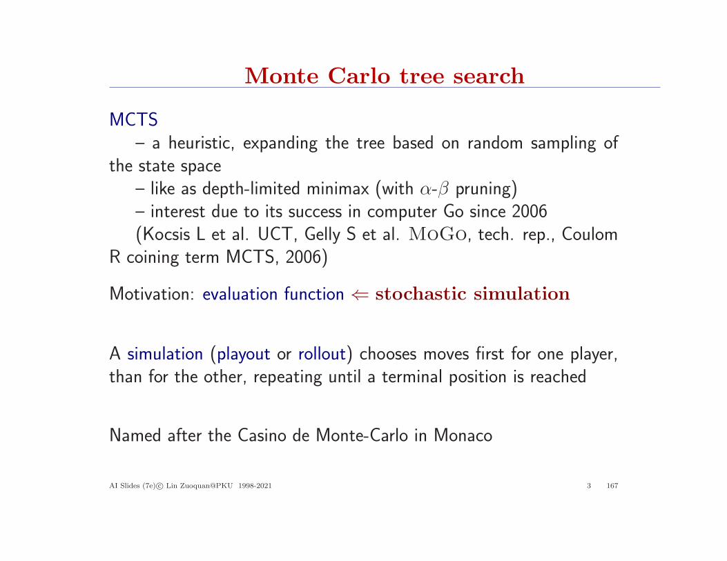
Monte Carlo tree search
MCTS– a heuristic, expanding the tree based on random sampling of
the state space– like as depth-limited minimax (with α-β pruning)– interest due to its success in computer Go since 2006(Kocsis L et al. UCT, Gelly S et al. MoGo, tech. rep., Coulom
R coining term MCTS, 2006)
Motivation: evaluation function ⇐ stochastic simulation
A simulation (playout or rollout) chooses moves first for one player,than for the other, repeating until a terminal position is reached
Named after the Casino de Monte-Carlo in Monaco
AI Slides (7e) c© Lin Zuoquan@PKU 1998-2021 3 167

MCTS
After 100 iterations (a) select moves for 27 wins for black out of 35playouts; (b) expand the selected node and do a playout ended in awin for black; (c) the results of playout are back-propagated up thetree (incremented 1)
AI Slides (7e) c© Lin Zuoquan@PKU 1998-2021 3 168
MCTS
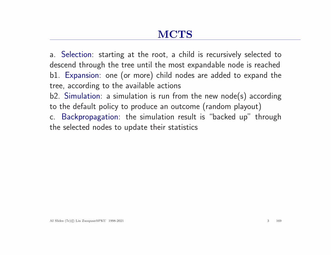
a. Selection: starting at the root, a child is recursively selected todescend through the tree until the most expandable node is reachedb1. Expansion: one (or more) child nodes are added to expand thetree, according to the available actionsb2. Simulation: a simulation is run from the new node(s) accordingto the default policy to produce an outcome (random playout)c. Backpropagation: the simulation result is “backed up” throughthe selected nodes to update their statistics
AI Slides (7e) c© Lin Zuoquan@PKU 1998-2021 3 169
MCTS policy
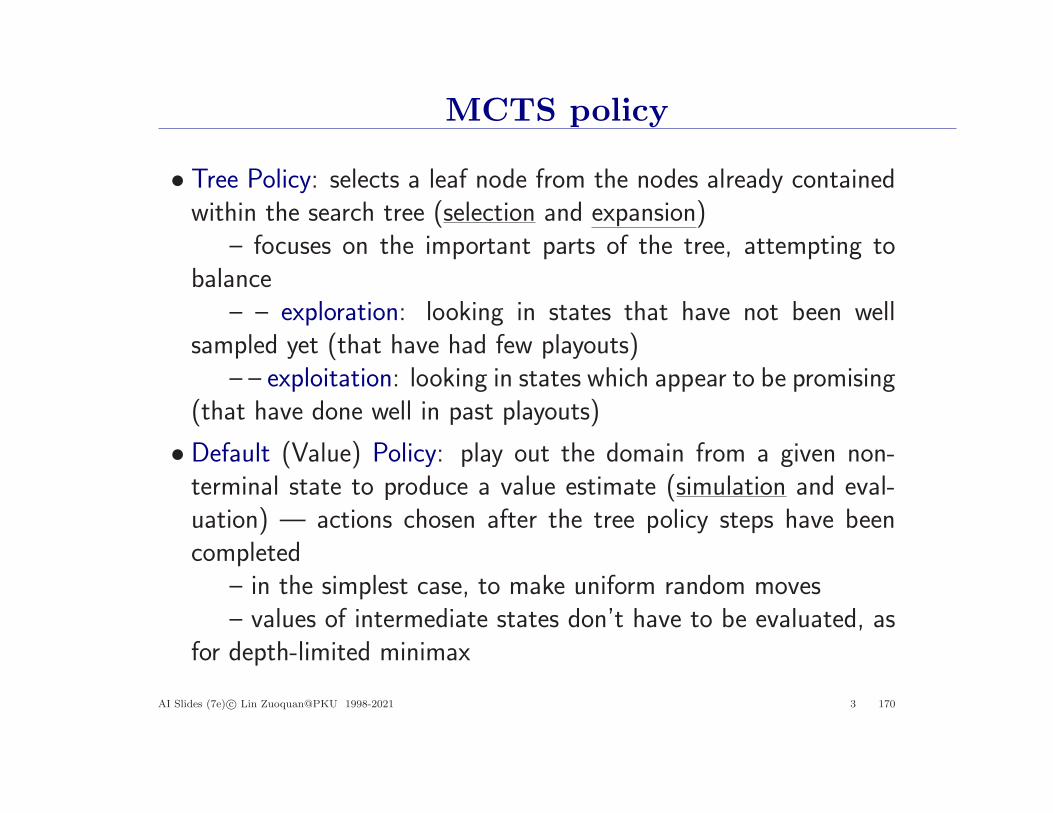
• Tree Policy: selects a leaf node from the nodes already containedwithin the search tree (selection and expansion)
– focuses on the important parts of the tree, attempting tobalance
– – exploration: looking in states that have not been wellsampled yet (that have had few playouts)
– – exploitation: looking in states which appear to be promising(that have done well in past playouts)
• Default (Value) Policy: play out the domain from a given non-terminal state to produce a value estimate (simulation and eval-uation) — actions chosen after the tree policy steps have beencompleted
– in the simplest case, to make uniform random moves– values of intermediate states don’t have to be evaluated, as
for depth-limited minimax
AI Slides (7e) c© Lin Zuoquan@PKU 1998-2021 3 170
Exploitation-exploration
Exploitation-exploration dilemma– one needs to balance the exploitation of the action currently
believed to be optimal with the exploration of other actions thatcurrently appear suboptimal but may turn out to be superior in thelong run
There are a number of variations of tree policy, say UCT,
Theorem: UCT allows MCTS to converge to the minimax tree and isthus optimal, given enough time (and memory)
AI Slides (7e) c© Lin Zuoquan@PKU 1998-2021 3 171
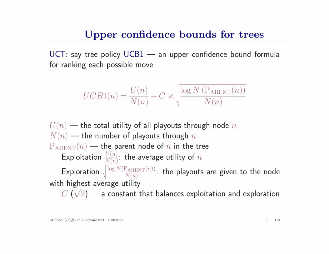
Upper confidence bounds for trees
UCT: say tree policy UCB1 — an upper confidence bound formulafor ranking each possible move
UCB1(n) =U(n)
N(n)+ C ×
√
√
√
√
√
√
√
logN (PARENT(n))
N(n)
U(n) — the total utility of all playouts through node nN(n) — the number of playouts through nPARENT(n) — the parent node of n in the tree
Exploitation U(n)N(n): the average utility of n
Exploration√
√
√
√
logN(PARENT(n))N(n) : the playouts are given to the node
with highest average utilityC (√2) — a constant that balances exploitation and exploration
AI Slides (7e) c© Lin Zuoquan@PKU 1998-2021 3 172
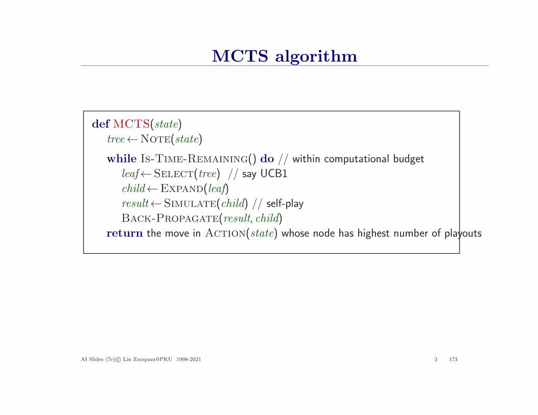
MCTS algorithm
def MCTS(state)
tree←Note(state)
while Is-Time-Remaining() do // within computational budget
leaf←Select(tree) // say UCB1
child←Expand(leaf)
result←Simulate(child) // self-play
Back-Propagate(result, child)
return the move in Action(state) whose node has highest number of playouts
AI Slides (7e) c© Lin Zuoquan@PKU 1998-2021 3 173

Properties of MCTS#
• Aheuristic: don’t need domain-specific knowledge (heuristic), ap-plicable to any domain modeled by a tree
• Anytime: all values up-to-date by backed up immediately allow toreturn an action from the root at any moment in time
• Asymmetric: The selection allows to favor more promising nodes(without allowing the selection probability of the other nodes to con-verge to zero), leading to an asymmetric tree over time
AI Slides (7e) c© Lin Zuoquan@PKU 1998-2021 3 174

Example: Alpha0
Go– MCTS had a dramatic effect on narrowing this gap, but is com-
petitive only on small boards (say, 9 × 9), or weak amateur levelplayer on the standard 19 × 19 board
– Pachi: open-source Go program, using MCTS, ranked at ama-teur 2 dan on KGS, that executes 100,000 simulations per move
Ref. Rimmel. A et al., Current Frontiers in Computer Go, IEEE Trans. Comp. Intell. AI Games, vol. 2, no. 4,
2010
AI Slides (7e) c© Lin Zuoquan@PKU 1998-2021 3 175
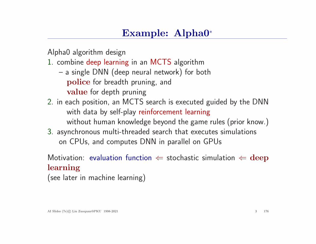
Example: Alpha0∗
Alpha0 algorithm design1. combine deep learning in an MCTS algorithm
– a single DNN (deep neural network) for bothpolice for breadth pruning, andvalue for depth pruning
2. in each position, an MCTS search is executed guided by the DNNwith data by self-play reinforcement learningwithout human knowledge beyond the game rules (prior know.)
3. asynchronous multi-threaded search that executes simulationson CPUs, and computes DNN in parallel on GPUs
Motivation: evaluation function ⇐ stochastic simulation ⇐ deep
learning
(see later in machine learning)
AI Slides (7e) c© Lin Zuoquan@PKU 1998-2021 3 176
Example: Alpha0
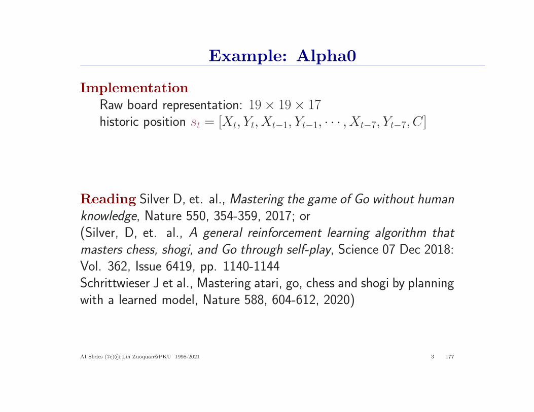
Implementation
Raw board representation: 19× 19× 17historic position st = [Xt, Yt, Xt−1, Yt−1, · · · , Xt−7, Yt−7, C]
Reading Silver D, et. al., Mastering the game of Go without human
knowledge, Nature 550, 354-359, 2017; or(Silver, D, et. al., A general reinforcement learning algorithm that
masters chess, shogi, and Go through self-play, Science 07 Dec 2018:Vol. 362, Issue 6419, pp. 1140-1144Schrittwieser J et al., Mastering atari, go, chess and shogi by planningwith a learned model, Nature 588, 604-612, 2020)
AI Slides (7e) c© Lin Zuoquan@PKU 1998-2021 3 177
Alpha0 algorithm: MCTS∗
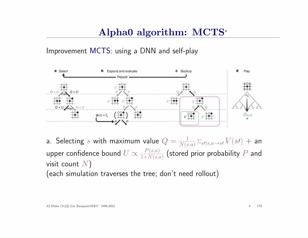
Improvement MCTS: using a DNN and self-play
a. Selecting s with maximum value Q = 1N(s,a)
∑
s′|s,a→s′ V (s′) + an
upper confidence bound U ∝ P (s,a)1+N(s,a) (stored prior probability P and
visit count N)(each simulation traverses the tree; don’t need rollout)
AI Slides (7e) c© Lin Zuoquan@PKU 1998-2021 3 178

Alpha0 algorithm: MCTS∗
Improvement MCTS: using a DNN and self-play
b. Expanding leaf and evaluating s by DNN (P (s, ·), V (s)) = fθ(s)c. Updating Q to track all V in the subtreed. Once completed, search probabilities π ∝ N(s, a)1/τ are returned(τ is a hyperparameter)
AI Slides (7e) c© Lin Zuoquan@PKU 1998-2021 3 179
Alpha0 pseudocode∗
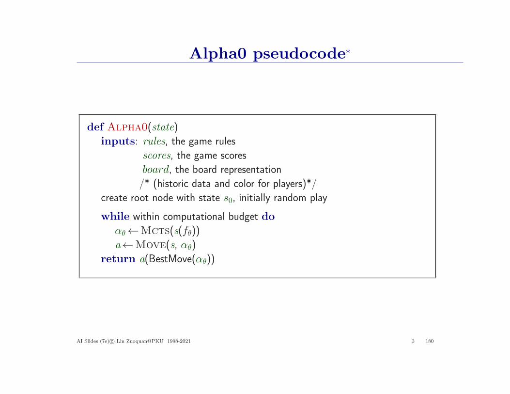
def Alpha0(state)
inputs: rules, the game rules
scores, the game scores
board, the board representation
/* (historic data and color for players)*/
create root node with state s0, initially random play
while within computational budget do
αθ←Mcts(s(fθ))
a←Move(s, αθ)
return a(BestMove(αθ))
AI Slides (7e) c© Lin Zuoquan@PKU 1998-2021 3 180
Alpha0 pseudocode∗
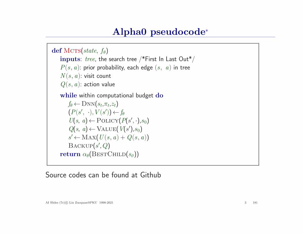
def Mcts(state, fθ)
inputs: tree, the search tree /*First In Last Out*/
P(s , a): prior probability, each edge (s , a) in tree
N (s , a): visit count
Q(s , a): action value
while within computational budget do
fθ←Dnn(st,πt,zt)
(P(s′, ·), V (s′))← fθU(s, a)←Policy(P(s′, ·),s0)Q(s, a)←Value(V(s′),s0)s′←Max(U (s , a) +Q(s , a))
Backup(s′,Q)
return αθ(BestChild(s0 ))
Source codes can be found at Github
AI Slides (7e) c© Lin Zuoquan@PKU 1998-2021 3 181

Complexity of Alpha0 algorithm
Go/Chess are NP-hard (“almost” in PSPACE) problems
Alpha0 do not reduce the complexity of Go/Chess, but– outperforms human in the complexity– – practical approach to handle NP-hard problems– obeys the complexity of MCTS and machine learning– – performance improvements from deep learning
by bigdata and computational power
Alpha0 toward N-steps optimization??– if so, a draw on Alpha0 vs. Alpha0 for Go/Chess
AI Slides (7e) c© Lin Zuoquan@PKU 1998-2021 3 182
Alpha0 vs. deep blue
Alpha0Go/Chess exceeded the performance of all other Go/Chessprograms, demonstrating that DNN provides a viable alternative toMonte Carlo simulation
Evaluated thousands of times fewer positions than Deep Blue did inmatch
– while Deep Blue relied on a handcrafted evaluation function,Alpha0’s neural network is trained purely through self-play reinforce-ment learning
AI Slides (7e) c© Lin Zuoquan@PKU 1998-2021 3 183
Example: Card
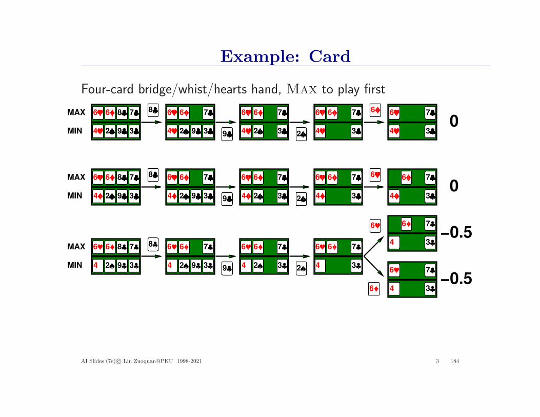
Four-card bridge/whist/hearts hand, Max to play first
8
9 2
66 6 8 7 6 6 7 6 6 7 6 6 7 6 7
4 2 9 3 4 2 9 3 4 2 3 4 3 4 30
6
4
8
9 2
6 6 8 7 6 6 7 6 6 7 6 6 7 7
2 9 3 2 9 3 2 3 3 30
4444
6
6
4
8
9 2
6 6 8 7 6 6 7 6 6 7
2 9 3 2 9 3 2 3
7
3
6
46 6 7
34446
6
7
34
−0.5
−0.5
MAX
MIN
MAX
MIN
MAX
MIN
AI Slides (7e) c© Lin Zuoquan@PKU 1998-2021 3 184
Imperfect information games in practice
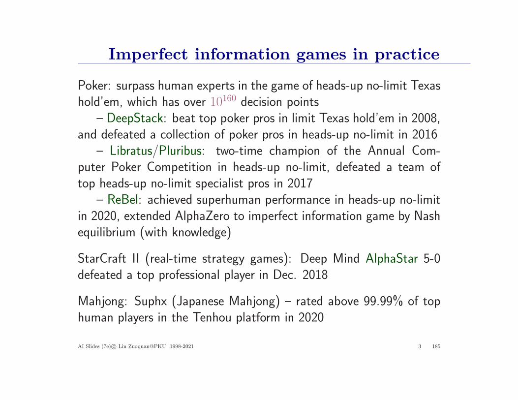
Poker: surpass human experts in the game of heads-up no-limit Texashold’em, which has over 10160 decision points
– DeepStack: beat top poker pros in limit Texas hold’em in 2008,and defeated a collection of poker pros in heads-up no-limit in 2016
– Libratus/Pluribus: two-time champion of the Annual Com-puter Poker Competition in heads-up no-limit, defeated a team oftop heads-up no-limit specialist pros in 2017
– ReBel: achieved superhuman performance in heads-up no-limitin 2020, extended AlphaZero to imperfect information game by Nashequilibrium (with knowledge)
StarCraft II (real-time strategy games): Deep Mind AlphaStar 5-0defeated a top professional player in Dec. 2018
Mahjong: Suphx (Japanese Mahjong) – rated above 99.99% of tophuman players in the Tenhou platform in 2020
AI Slides (7e) c© Lin Zuoquan@PKU 1998-2021 3 185

Imperfect information games in practice
Imperfect information games involves obstacles not present in classicboard games like go, but
which are present in many real-world applications, such as nego-tiation, auctions, security, weather prediction and climate modellingetc.
AI Slides (7e) c© Lin Zuoquan@PKU 1998-2021 3 186
Metaheuristic∗
Metaheuristic: higher-level procedure or heuristicto find a heuristic for optimization ⇐ local seache.g., simulated annealing
Metalevel vs. object-level state spaceEach state in a metalevel state space captures the internal state
of a program that is searching in an object-level state space
An agent can learn how to search better– metalevel learning algorithm can learn from experiences to avoid
exploring unpromising subtrees– learning is to minimize the total cost of problem solvingspecially, learning admissible heuristics from example, e.g., 8-
puzzle
AI Slides (7e) c© Lin Zuoquan@PKU 1998-2021 3 187
Tabu search
Tabu search is a metaheuristic employing local searchresolving stuck in local minimum or plateause.g., Hill-Climbing
Tabu (forbidden) uses memory structures (tabulist) that describethe visited solutions or user-provided rules
– to discourage the search from coming back to previously-visitedsolutions
– depended certain short-term period or violated a rule (markedas “tab”) to avoid repeat
AI Slides (7e) c© Lin Zuoquan@PKU 1998-2021 3 188

Tabu search algorithm
def Tabu-Search( solution)
persistent: tabulist, a memory structure for states visited, initially empty
solution-best← solution
while not Stopping-Condition
Candidate← null
best.Candidate-List← null
for solution.Candidate in solution.Neighborhood
if not tabulist.Contains(solution.Candidate) and
Fitness(solution.Candidate)> Fitness(best.Candidate)
best.Candidate← solution.Candidate
solution← best.Candidate
if Fitness(best.Candidate) > Fitness(solution-best)
solution-best← best.Candidate
tabuist.Push(best.Candidate)
if tabulist.Size > MaxTabuSize
tabulist.RemoveFirst()
return solution-best
AI Slides (7e) c© Lin Zuoquan@PKU 1998-2021 3 189

Searching search∗
Researchers have taken inspiration for search (and optimization) al-gorithms from a wide variety of fields
– metallurgy (simulated annealing)– biology (genetic algorithms)– economics (market-based algorithms)– entomology (ant colony)– neurology (neural networks)– animal behavior (reinforcement learning)– mountaineering (hill climbing)– politics (struggle forms), and others
Ref: Pearl, J (1984), Heuristics: Intelligent Search Strategies for Computer Problem Solving, Addison- Wesley
Is there a general problem solver to generality of intelligence?? – NO
AI Slides (7e) c© Lin Zuoquan@PKU 1998-2021 3 190