Bandit Algorithms for Tree Search

Bandit Algorithms for Tree Search

Pierre-Arnaud Coquelin, Remi Munos

To cite this version:

Pierre-Arnaud Coquelin, Remi Munos. Bandit Algorithms for Tree Search. [Research Report]RR-6141, INRIA. 2007, pp.20. <inria-00136198v2>

HAL Id: inria-00136198

https://hal.inria.fr/inria-00136198v2

Submitted on 13 Mar 2007

HAL is a multi-disciplinary open accessarchive for the deposit and dissemination of sci-entific research documents, whether they are pub-lished or not. The documents may come fromteaching and research institutions in France orabroad, or from public or private research centers.

L’archive ouverte pluridisciplinaire HAL, estdestinee au depot et a la diffusion de documentsscientifiques de niveau recherche, publies ou non,emanant des etablissements d’enseignement et derecherche francais ou etrangers, des laboratoirespublics ou prives.

https://hal.archives-ouvertes.fr

https://hal.inria.fr/inria-00136198v2

inria

-001

3619

8, v

ersi

on 2

- 1

3 M

ar 2

007

appor t de r ech er ch e

ISS

N02

49-6

399

ISR

NIN

RIA

/RR

--61

41--

FR

+E

NG

Thème COG

INSTITUT NATIONAL DE RECHERCHE EN INFORMATIQUE ET EN AUTOMATIQUE


Pierre-Arnaud Coquelin — Rémi Munos

N° 6141

March 2007

Unité de recherche INRIA FutursParc Club Orsay Université, ZAC des Vignes,

4, rue Jacques Monod, 91893 ORSAY Cedex (France)Téléphone : +33 1 72 92 59 00 — Télécopie : +33 1 60 19 66 08


Pierre-Arnaud Coquelin ∗, Remi Munos †

Theme COG — Systemes cognitifsProjet SequeL

Rapport de recherche n° 6141 — March 2007 — 19 pages

Abstract: Bandit based methods for tree search have recently gained popularity whenapplied to huge trees, e.g. in the game of go [GWMT06]. The UCT algorithm [KS06], atree search method based on Upper Confidence Bounds (UCB) [ACBF02], is believed toadapt locally to the effective smoothness of the tree. However, we show that UCT is too“optimistic” in some cases, leading to a regret Ω(exp(exp(D))) where D is the depth ofthe tree. We propose alternative bandit algorithms for tree search. First, a modificationof UCT using a confidence sequence that scales exponentially with the horizon depth isproven to have a regret O(2D

√n), but does not adapt to possible smoothness in the tree.

We then analyze Flat-UCB performed on the leaves and provide a finite regret bound withhigh probability. Then, we introduce a UCB-based Bandit Algorithm for Smooth Treeswhich takes into account actual smoothness of the rewards for performing efficient “cuts” ofsub-optimal branches with high confidence. Finally, we present an incremental tree searchversion which applies when the full tree is too big (possibly infinite) to be entirely representedand show that with high probability, essentially only the optimal branches is indefinitelydeveloped. We illustrate these methods on a global optimization problem of a Lipschitzfunction, given noisy data.

Key-words: Bandit algorithms, tree search, exploration-exploitation tradeoff, upper con-fidence bounds, minimax game, reinforcement learning

∗ CMAP, Ecole Polytechnique, [email protected]† SequeL, INRIA, [email protected]


Resume : Les methodes de recherche arborescentes utilisant des algorithmes de banditont recemment connu une forte popularite, pour leur capacite de traiter des grands arbres,par exemple pour le jeu de go [GWMT06]. Il est connu que l’algorithme UCT [KS06], unemethode de recherche arborescente basees sur des intervalles de confiance (algorithme UpperConfidence Bounds (UCB) de [ACBF02]), s’adapte locallement a la profondeur effective del’arbre. Cependant, nous montrons ici que UCT peut etre trop “optimiste” dans certainscas, menant a un regret Ω(exp(exp(D))) ou D est la profondeur de l’arbre. Nous proposonsplusieurs alternatives d’algorithmes de bandit pour la recherche arborescente. Tout d’abord,nous proposons une modification d’UCT utilisant un intervalle de confiance qui croit exponentiellementavec la profondeur de l’horizon de l’arbre, et montrons qu’il mene a un regret O(2D

√n) mais

ne s’adapte pas a la regularite de l’arbre. Puis nous analysons un algorithme Flat-UCB debandit de type UCB directement sur les feuilles et prouvons une borne finie (independantede n) sur le regret avec forte probabilite. Ensuite, nous introduisons un algorithme BanditAlgorithm for Smooth Trees qui prend en compte d’eventuelles regularites dans l’arbre pourrealiser des “coupes” efficaces de branches sous-optimale avec grande confiance. Enfin,nous presentons une version incrementale de recherche arborescente qui s’applique lorsquel’arbre est trop grand (voire infini) pour pouvoir etre represente entierement, et montronsqu’essentiellement, et avec forte probabilite, seule la branche optimale est indefinimentdeveloppee. Nous illustrons ces methodes sur un probleme d’optimisation d’une fonctionLipschitzienne, a partir de donnees bruitees.

Mots-cles : Algorithmes de bandit, recherche arborescente, compromis exploration-exploitation, bornes superieures d’intervalles de confiance, jeux minimax, apprentissage parrenforcement

Bandit Algorithms for Tree Search 3

1 Introduction

Bandit algorithms have been used recently for tree search, because of their efficient trade-offbetween exploration of the most uncertain branches and exploitation of the most promisingones, leading to very promising results in dealing with huge trees (e.g. the go programMoGo, see [GWMT06]). In this paper we focus on Upper Confidence Bound (UCB) banditalgorithms [ACBF02] applied to tree search, such as UCT (Upper Confidence Bounds appliedto Trees) [KS06]. The general procedure is described by Algorithm 1 and depends on theway the upper-bounds Bi,p,ni for each node i are maintained.

Algorithm 1 Bandit Algorithm for Tree Search

for n ≥ 1 do

Run n-th trajectory from the root to a leaf:

Set the current node i0 to the rootfor d = 1 to D do

Select node id as the children j of node id−1 that maximizes Bj,nid−1,nj

end for

Receive reward xniid∼ XiD

Update the nodes visited by this trajectory:

for d = D to 0 do

Update the number of visits: nid= nid

+ 1Update the bound Bid,nid−1

,nid

end for

end for

A trajectory is a sequence of nodes from the root to a leaf, where at each node, thenext node is chosen as the one maximizing its B value among the children. A reward isreceived at the leaf. After a trajectory is run, the B values of each node in the trajectoryare updated. In the case of UCT, the upper-bound Bi,p,ni of a node i, given that the nodehas already been visited ni times and its parent’s node p times, is the average of the rewardsxt1≤t≤ni obtained from that node Xi,ni = 1

ni

∑ni

t=1 xt plus a confidence interval, derivedfrom a Chernoff-Hoeffding bound (see e.g. [GDL96]):

Bi,p,ni

def= Xi,ni +

√

2 log(p)

ni(1)

In this paper we consider a max search (the minimax problem is a direct generalizationof the results presented here) in binary trees (i.e. there are 2 actions in each node), althoughthe extension to more actions is straightforward. Let a binary tree of depth D where at eachleaf i is assigned a random variable Xi, with bounded support [0, 1], whose law is unknown.Successive visits of a leaf i yield a sequence of independent and identically distributed (i.i.d.)samples xi,t ∼ Xi, called rewards, or payoff. The value of a leaf i is its expected reward:

RR n° 6141

4 Coquelin & Munos

µidef= EXi. Now we define the value of any node i as the maximal value of the leaves in the

branch starting from node i. Our goal is to compute the value µ∗ of the root.An optimal leaf is a leaf having the largest expected reward. We will denote by ∗

quantities related to an optimal node. For example µ∗ denote maxi µi. An optimal branchis a sequence of nodes from the root to a leaf, having the µ∗ value. We define the regret upto time n as the difference between the optimal expected payoff and the sum of obtainedrewards:

Rndef= µ∗ −

n∑

t=1

xit,t,

where it is the chosen leaf at round t. We also define the pseudo-regret up to time n:

Rndef= µ∗ −

n∑

t=1

µit =∑

j∈L

nj∆j ,

where L is the set of leaves, ∆jdef= µ∗ − µj , and nj is the random variable that counts

the number of times leaf j has been visited up to time n. The pseudo-regret may thus beanalyzed by estimating the number of times each sub-optimal leaf is visited.

In tree search, our goal is thus to find an exploration policy of the branches such as tominimize the regret, in order to select an optimal leaf as fast as possible. Now, thanks to asimple contraction of measure phenomenon, the regret per bound Rn/n turns out to be veryclose to the pseudo regret per round Rn/n. Indeed, using Azuma’s inequality for martingaledifference sequences (see Proposition 1), with probability at least 1 − β, we have at time n,

1

n|Rn − Rn| ≤

√

2 log(2/β)

n.

The fact that R(n)−Rn is a martingale difference sequence comes from the property that,given the filtration Ft−1 defined by the random samples up to time t− 1, the expectation ofthe next reward Ext is conditioned to the leaf it chosen by the algorithm: E[xt|Ft−1] = µit .Thus Rn − Rn =

∑nt=1 xt − µit with E[xt − µit |Ft−1] = 0. Hence, we will only focus on

providing high probability bounds on the pseudo-regret.First, we analyze the UCT algorithm defined by the upper confidence bound (1). We show

that its behavior is risky and may lead to a regret as bad as Ω(exp(· · · exp(D) · · · )) (D − 1composed exponential functions). We modify the algorithm by increasing the explorationsequence, defining:

Bi,p,ni

def= Xi,ni +

√√p

ni. (2)

This yields an improved worst-case behavior over regular UCT, but the regret may stillbe as bad as Ω(exp(exp(D))) (see Section 2). We then propose in Section 3 a modified UCTbased on the bound (2), where the confidence interval is multiplied by a factor that scalesexponentially with the horizon depth. We derive a worst-case regret O(2D/

√n) with high

INRIA


probability. However this algorithm does not adapt to the effective smoothness of the tree,if any.

Next we analyze the Flat-UCB algorithm, which simply performs UCB directly on theleaves. With a slight modification of the usual confidence sequence, we show in Section4 that this algorithm has a finite regret O(2D/∆) (where ∆ = mini,∆i>0 ∆i) with highprobability.

In Section 5, we introduce a UCB-based algorithm, called Bandit Algorithm for SmoothTrees, which takes into account actual smoothness of the rewards for performing efficient“cuts” of sub-optimal branches based on concentration inequality. We give a numericalexperiment for the problem of optimizing a Lipschitz function given noisy observations.

Finally, in Section 6 we present and analyze a growing tree search, which builds incre-mentally the tree by expanding, at each iteration, the most promising node. This methodis memory efficient and well adapted to search in large (possibly infinite) trees.

Additional notations: Let L denotes the set of leaves and S the set of sub-optimal leaves.For any node i, we write L(i) the set of leaves in the branch starting from node i. For anynode i, we write ni the number of times node i has been visited up to round n, and wedefine the cumulative rewards:

Xi,ni =1

ni

∑

j∈L(i)

njXj,nj ,

the cumulative expected rewards:

Xi,ni =1

ni

∑

j∈L(i)

njµj ,

and the pseudo-regret:

Ri,ni =∑

j∈L(i)

nj(µi − µj).

2 Lower regret bound for UCT

The UCT algorithm introduced in [KS06] is believed to adapt automatically to the effective(and a priori unknown) smoothness of the tree: If the tree possesses an effective depth d < D(i.e. if all leaves of a branch starting from a node of depth d have the same value) then itsregret will be equal to the regret of a tree of depth d. First, we notice that the bound (1) isnot a true upper confidence bound on the value µi of a node i since the rewards received atnode i are not identically distributed (because the chosen leaves depend on a non-stationarynode selection process). However, due to the increasing confidence term log(p) when a nodeis not chosen, all nodes will be infinitely visited, which guarantees an asymptotic regret ofO(log(n)). However the transitory phase may last very long.

RR n° 6141

6 Coquelin & Munos

Indeed, consider the example illustrated in Figure 1. The rewards are deterministic andfor a node of depth d in the optimal branch (obtained after choosing d times action 1), ifaction 2 is chosen, then a reward of D−d

D is received (all leaves in this branch have the samereward). If action 1 is chosen, then this moves to the next node in the optimal branch. Atdepth D− 1, action 1 yields reward 1 and action 2, reward 0. We assume that when a nodeis visited for the first time, the algorithm starts by choosing action 2 before choosing action1.

1

0

(D−1)/D

(D−2)/D

1/D

2/D1

1

21

2

2

1

21

2

Figure 1: A bad example for UCT. From the root (left node), action 2 leads to a node fromwhich all leaves yield reward D−1

D . The optimal branch consists in choosing always action1, which yields reward 1. In the beginning, the algorithm believes the arm 2 is the best,spending most of its times exploring this branch (as well as all other sub-optimal branches).It takes Ω(exp(exp(D))) rounds to get the 1 reward!

We now establish a lower bound on the number of times suboptimal rewards are receivedbefore getting the optimal 1 reward for the first time. Write n the first instant when theoptimal leaf is reached. Write nd the number of times the node (also written d making aslight abuse of notation) of depth d in the optimal branch is reached. Thus n = n0 andnD = 1. At depth D − 1, we have nD−1 = 2 (since action 2 has been chosen once in nodeD − 1).

We consider both the logarithmic confidence sequence used in (1) and the square rootsequence in (2). Let us start with the square root confidence sequence (2). At depth d − 1,since the optimal branch is followed by the n-th trajectory, we have (writting d′ the node

INRIA


resulting from action 2 in the node d − 1):

Xd′,nd′+

√√nd−1

nd′

≤ Xd,nd+

√√nd−1

nd.

But Xd′,nd′= (D − d)/D and Xd,nd

≤ (D − (d + 1))/D since the 1 reward has not beenreceived before. We deduce that

1

D≤

√√nd−1

nd.

Thus for the square root confidence sequence, we have nd−1 ≥ n2d/D4. Now, by induction,

n ≥ n21

D4≥ n22

2

D4(1+2)≥ n23

3

D4(1+2+3)≥ · · · ≥ n2D−1

D−1

D2D(D−1)

Since nD−1 = 2, we obtain n ≥ 22D−1

D2D(D−1) . This is a double exponential dependencyw.r.t. D. For example, for D = 20, we have n ≥ 10156837. Consequently, the regret is alsoΩ(exp(exp(D))).

Now, the usual logarithmic confidence sequence defined by (1) yields an even worstlower bound on the regret since we may show similarly that nd−1 ≥ exp(nd/(2D2)) thusn ≥ exp(exp(· · · exp(2) · · · )) (composition of D − 1 exponential functions).

Thus, although UCT algorithm has asymptotically regret O(log(n)) in n, (or O(√

n) forthe square root sequence), the transitory regret is Ω(exp(exp(· · · exp(2) · · · ))) (or Ω(exp(exp(D)))in the square root sequence).

The reason for this bad behavior is that the algorithm is too optimistic (it does notexplore enough and may take a very long time to discover good branches that looked initiallybad) since the bounds (1) and (2) are not true upper bounds.

3 Modified UCT

We modify the confidence sequence to explore more the nodes close to the root that theleaves, taking into account the fact that the time needed to decrease the bias (µi −E[Xi,ni ])at a node i of depth d increases with the depth horizon (D− d). For such a node i of depthd, we define the upper confidence bound:

Bi,ni

def= Xi,ni + (kd + 1)

√

2 log(β−1ni )

ni+

k′d

ni, (3)

where βndef= β

2Nn(n+1) with N = 2D+1 − 1 the number of nodes in the tree, and the

coefficients:

kddef=

1 +√

2√2

[

(1 +√

2)D−d − 1]

(4)

k′d

def= (3D−d − 1)/2

RR n° 6141

8 Coquelin & Munos

Notice that we used a simplified notation, writing Bi,ni instead of Bi,p,ni since the bounddoes not depend on the number of visits of the parent’s node.

Theorem 1. Let β > 0. Consider Algorithm 1 with the upper confidence bound (3). Then,with probability at least 1 − β, for all n ≥ 1, the pseudo-regret is bounded by

Rn ≤ 1 +√

2√2

[

(1 +√

2)D − 1]

√

2 log(β−1n )n +

3D − 1

2

Proof. We first remind Azuma’s inequality (see [GDL96]):

Proposition 1. Let f be a Lipschitz function of n independent random variables such thatf −Ef =

∑ni=1 di where (di)1≤i≤n is a martingale difference sequence, i.e.: E[di|Fi−1] = 0,

1 ≤ i ≤ n, such that ||di||∞ ≤ 1/n. Then for every ǫ > 0,

P (|f − Ef | > ǫ) ≤ 2 exp(

− nǫ2/2).

We apply Azuma’s inequality to the random variables Yi,ni and Zi,ni , defined respectively,

for all nodes i, by Yi,ni

def= Xi,ni − Xi,ni , and for all non-leaf nodes i, by

Zi,ni

def=

1

ni(ni1Yi1,ni1

− ni2Yi2,ni2),

where i1 and i2 denote the children of i.Since at each round t ≤ ni, the choice of the next leaf only depends on the random

samples drawn at previous times s < t, we have E[Yi,t|Ft−1] = 0 and E[Zi,t|Ft−1] = 0, (i.e..Y and Z are martingale difference sequences), and Azuma’s inequality gives that, for anynode i, for any ni, for any ǫ > 0, P (|Yi,ni | > ǫ) ≤ 2 exp

(

− niǫ2/2) and P (|Zi,ni | > ǫ) ≤

2 exp(

− niǫ2/2).

We now define a confidence level cni such that with probability at least 1−β, the randomvariables Yi,ni and Zi,ni belong to their confidence intervals for all nodes and for all times.More precisely, let E be the event under which, for all ni ≥ 1, for all nodes i, |Yi,ni | ≤ cni

and for all non-leaf nodes i, |Zi,ni | ≤ cni . Then, by defining

cndef=

√

2 log(β−1n )

n, with βn

def=

β

2Nn(n + 1),

the event E holds with probability at least 1 − β.Indeed, from an union bound argument, there are at most 2N inequalities (for each node,

one for Y , one for Z) of the form:

P (|Yi,ni | > cni , ∀ni ≥ 1) ≤∑

ni≥1

β

2Nni(ni + 1)=

β

2N.

INRIA


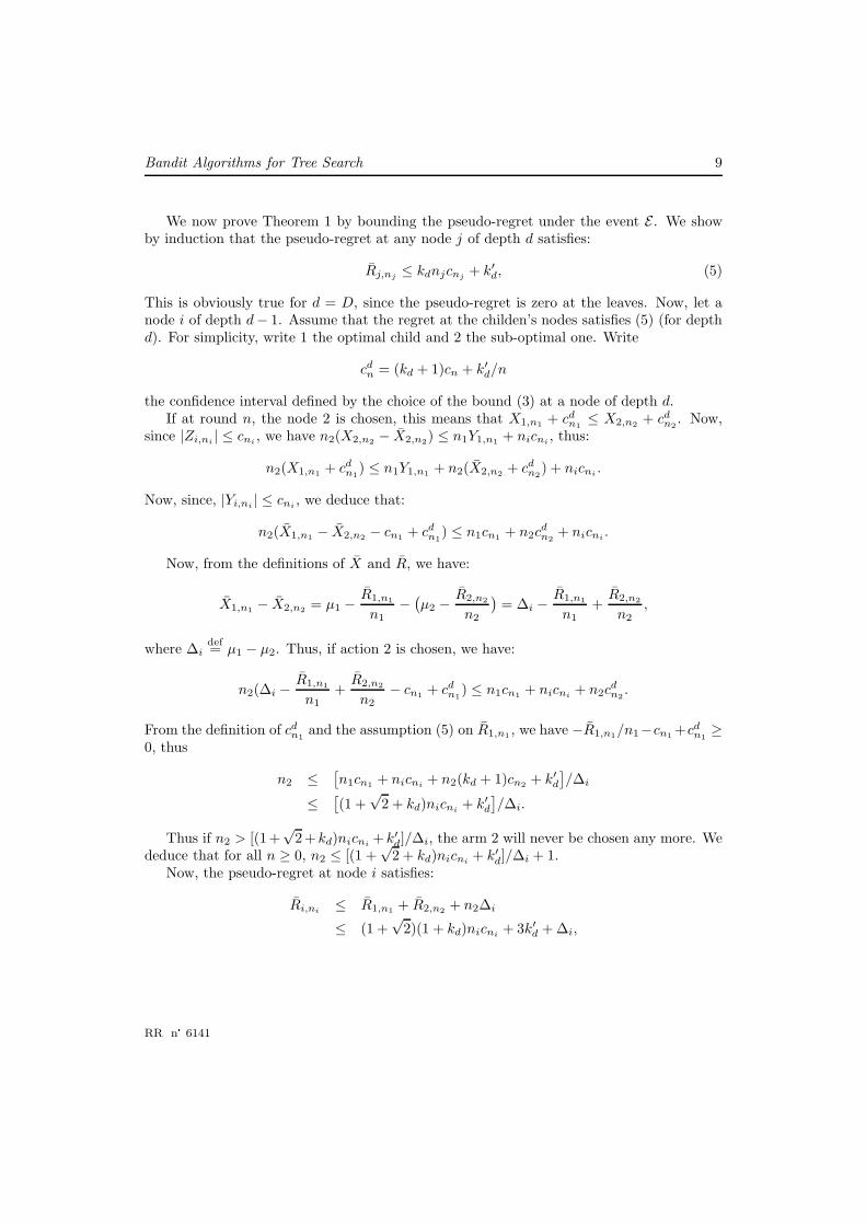
We now prove Theorem 1 by bounding the pseudo-regret under the event E . We showby induction that the pseudo-regret at any node j of depth d satisfies:

Rj,nj ≤ kdnjcnj + k′d, (5)

This is obviously true for d = D, since the pseudo-regret is zero at the leaves. Now, let anode i of depth d− 1. Assume that the regret at the childen’s nodes satisfies (5) (for depthd). For simplicity, write 1 the optimal child and 2 the sub-optimal one. Write

cdn = (kd + 1)cn + k′

d/n

the confidence interval defined by the choice of the bound (3) at a node of depth d.If at round n, the node 2 is chosen, this means that X1,n1 + cd

n1≤ X2,n2 + cd

n2. Now,

since |Zi,ni | ≤ cni , we have n2(X2,n2 − X2,n2) ≤ n1Y1,n1 + nicni , thus:

n2(X1,n1 + cdn1

) ≤ n1Y1,n1 + n2(X2,n2 + cdn2

) + nicni .

Now, since, |Yi,ni | ≤ cni , we deduce that:

n2(X1,n1 − X2,n2 − cn1 + cdn1

) ≤ n1cn1 + n2cdn2

+ nicni .

Now, from the definitions of X and R, we have:

X1,n1 − X2,n2 = µ1 −R1,n1

n1−

(

µ2 −R2,n2

n2

)

= ∆i −R1,n1

n1+

R2,n2

n2,

where ∆idef= µ1 − µ2. Thus, if action 2 is chosen, we have:

n2(∆i −R1,n1

n1+

R2,n2

n2− cn1 + cd

n1) ≤ n1cn1 + nicni + n2c

dn2

.

From the definition of cdn1

and the assumption (5) on R1,n1 , we have −R1,n1/n1−cn1 +cdn1

≥0, thus

n2 ≤[

n1cn1 + nicni + n2(kd + 1)cn2 + k′d

]

/∆i

≤[

(1 +√

2 + kd)nicni + k′d

]

/∆i.

Thus if n2 > [(1+√

2+ kd)nicni + k′d]/∆i, the arm 2 will never be chosen any more. We

deduce that for all n ≥ 0, n2 ≤ [(1 +√

2 + kd)nicni + k′d]/∆i + 1.

Now, the pseudo-regret at node i satisfies:

Ri,ni ≤ R1,n1 + R2,n2 + n2∆i

≤ (1 +√

2)(1 + kd)nicni + 3k′d + ∆i,

RR n° 6141

10 Coquelin & Munos

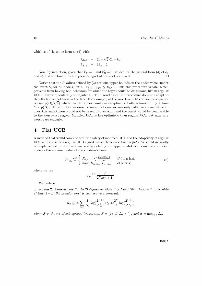
which is of the same form as (5) with

kd−1 = (1 +√

2)(1 + kd)

k′d−1 = 3k′

d + 1.

Now, by induction, given that kD = 0 and k′D = 0, we deduce the general form (4) of kd

and k′d and the bound on the pseudo-regret at the root for d = 0.

Notice that the B values defined by (3) are true upper bounds on the nodes value: underthe event E , for all node i, for all ni ≥ 1, µi ≤ Bi,ni . Thus this procedure is safe, whichprevents from having bad behaviors for which the regret could be disastrous, like in regularUCT. However, contrarily to regular UCT, in good cases, the procedure does not adapt tothe effective smoothness in the tree. For example, at the root level, the confidence sequenceis O(exp(D)/

√n) which lead to almost uniform sampling of both actions during a time

O(exp(D)). Thus, if the tree were to contain 2 branches, one only with zeros, one only withones, this smoothness would not be taken into account, and the regret would be comparableto the worst-case regret. Modified UCT is less optimistic than regular UCT but safer in aworst-case scenario.

4 Flat UCB

A method that would combine both the safety of modified UCT and the adaptivity of regularUCT is to consider a regular UCB algorithm on the leaves. Such a flat UCB could naturallybe implemented in the tree structure by defining the upper confidence bound of a non-leafnode as the maximal value of the children’s bound:

Bi,ni

def=

Xi,ni +

√

2 log(β−1ni

)

niif i is a leaf,

max[

Bi1,ni1 , Bi2,ni2

]

otherwise.(6)

where we use

βndef=

β

2Dn(n + 1).

We deduce:

Theorem 2. Consider the flat UCB defined by Algorithm 1 and (6). Then, with probabilityat least 1 − β, the pseudo-regret is bounded by a constant:

Rn ≤ 40∑

i∈S

1

∆ilog(

2D+1

∆2i β

) ≤ 402D

∆log(

2D+1

∆2β),

where S is the set of sub-optimal leaves, i.e.. S = i ∈ L, ∆i > 0, and ∆ = mini∈S ∆i.

INRIA


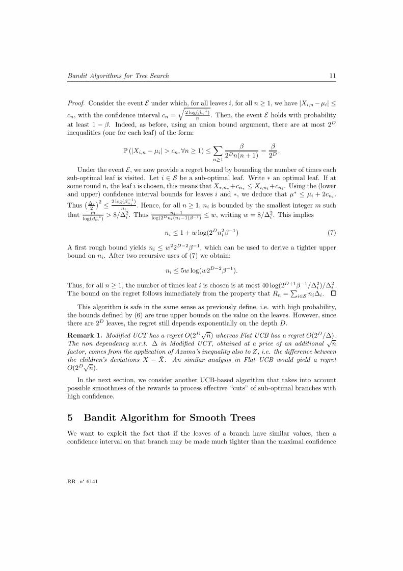
Proof. Consider the event E under which, for all leaves i, for all n ≥ 1, we have |Xi,n−µi| ≤cn, with the confidence interval cn =

√

2 log(β−1n )

n . Then, the event E holds with probability

at least 1 − β. Indeed, as before, using an union bound argument, there are at most 2D

inequalities (one for each leaf) of the form:

P (|Xi,n − µi| > cn, ∀n ≥ 1) ≤∑

n≥1

β

2Dn(n + 1)=

β

2D.

Under the event E , we now provide a regret bound by bounding the number of times eachsub-optimal leaf is visited. Let i ∈ S be a sub-optimal leaf. Write ∗ an optimal leaf. If atsome round n, the leaf i is chosen, this means that X∗,n∗

+cn∗≤ Xi,ni +cni . Using the (lower

and upper) confidence interval bounds for leaves i and ∗, we deduce that µ∗ ≤ µi + 2cni .

Thus(

∆i

2

)2 ≤ 2 log(β−1ni

)

ni. Hence, for all n ≥ 1, ni is bounded by the smallest integer m such

that mlog(β−1

m )> 8/∆2

i . Thus ni−1log(2Dni(ni−1)β−1) ≤ w, writing w = 8/∆2

i . This implies

ni ≤ 1 + w log(2Dn2i β

−1) (7)

A first rough bound yields ni ≤ w22D−2β−1, which can be used to derive a tighter upperbound on ni. After two recursive uses of (7) we obtain:

ni ≤ 5w log(w2D−2β−1).

Thus, for all n ≥ 1, the number of times leaf i is chosen is at most 40 log(2D+1β−1/∆2i )/∆2

i .The bound on the regret follows immediately from the property that Rn =

∑

i∈S ni∆i.

This algorithm is safe in the same sense as previously define, i.e. with high probability,the bounds defined by (6) are true upper bounds on the value on the leaves. However, sincethere are 2D leaves, the regret still depends exponentially on the depth D.

Remark 1. Modified UCT has a regret O(2D√

n) whereas Flat UCB has a regret O(2D/∆).The non dependency w.r.t. ∆ in Modified UCT, obtained at a price of an additional

√n

factor, comes from the application of Azuma’s inequality also to Z, i.e. the difference betweenthe children’s deviations X − X. An similar analysis in Flat UCB would yield a regretO(2D√

n).

In the next section, we consider another UCB-based algorithm that takes into accountpossible smoothness of the rewards to process effective “cuts” of sub-optimal branches withhigh confidence.

5 Bandit Algorithm for Smooth Trees

We want to exploit the fact that if the leaves of a branch have similar values, then aconfidence interval on that branch may be made much tighter than the maximal confidence

RR n° 6141

12 Coquelin & Munos

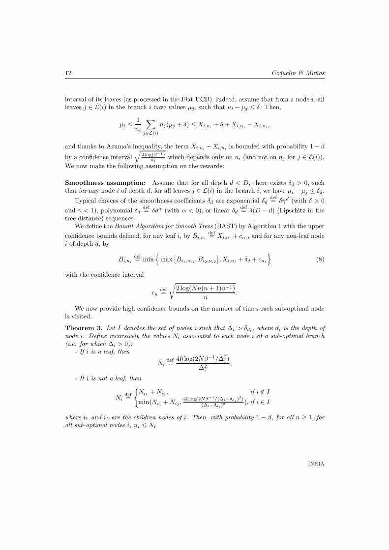
interval of its leaves (as processed in the Flat UCB). Indeed, assume that from a node i, allleaves j ∈ L(i) in the branch i have values µj , such that µi − µj ≤ δ. Then,

µi ≤1

ni

∑

j∈L(i)

nj(µj + δ) ≤ Xi,ni + δ + Xi,ni − Xi,ni ,

and thanks to Azuma’s inequality, the term Xi,ni −Xi,ni is bounded with probability 1− β

by a confidence interval√

2 log(β−1)ni

which depends only on ni (and not on nj for j ∈ L(i)).

We now make the following assumption on the rewards:

Smoothness assumption: Assume that for all depth d < D, there exists δd > 0, suchthat for any node i of depth d, for all leaves j ∈ L(i) in the branch i, we have µi − µj ≤ δd.

Typical choices of the smoothness coefficients δd are exponential δddef= δγd (with δ > 0

and γ < 1), polynomial δddef= δdα (with α < 0), or linear δd

def= δ(D − d) (Lipschitz in the

tree distance) sequences.We define the Bandit Algorithm for Smooth Trees (BAST) by Algorithm 1 with the upper

confidence bounds defined, for any leaf i, by Bi,ni

def= Xi,ni + cni , and for any non-leaf node

i of depth d, by

Bi,ni

def= min

max[

Bi1,ni1 , Bi2,ni2

]

, Xi,ni + δd + cni

(8)

with the confidence interval

cndef=

√

2 log(Nn(n + 1)β−1)

n.

We now provide high confidence bounds on the number of times each sub-optimal nodeis visited.

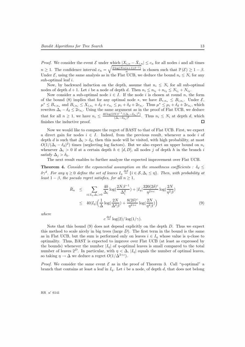
Theorem 3. Let I denotes the set of nodes i such that ∆i > δdi , where di is the depth ofnode i. Define recursively the values Ni associated to each node i of a sub-optimal branch(i.e. for which ∆i > 0):

- If i is a leaf, then

Nidef=

40 log(2Nβ−1/∆2i )

∆2i

,

- It i is not a leaf, then

Nidef=

Ni1 + Ni2 , if i /∈ I

min(Ni1 + Ni2 ,40 log(2Nβ−1/(∆i−δdi

)2)

(∆i−δdi)2 ), if i ∈ I

where i1 and i2 are the children nodes of i. Then, with probability 1 − β, for all n ≥ 1, forall sub-optimal nodes i, ni ≤ Ni.

INRIA


Proof. We consider the event E under which |Xi,n − Xi,n| ≤ cn for all nodes i and all times

n ≥ 1. The confidence interval cn =√

2 log(Nn(n+1)β−1)n is chosen such that P (E) ≥ 1 − β.

Under E , using the same analysis as in the Flat UCB, we deduce the bound ni ≤ Ni for anysub-optimal leaf i.

Now, by backward induction on the depth, assume that ni ≤ Ni for all sub-optimalnodes of depth d + 1. Let i be a node of depth d. Then ni ≤ ni1 + ni2 ≤ Ni1 + Ni2 .

Now consider a sub-optimal node i ∈ I. If the node i is chosen at round n, the formof the bound (8) implies that for any optimal node ∗, we have B∗,n∗

≤ Bi,ni . Under E ,µ∗ ≤ B∗,n∗

and Bi,ni ≤ Xi,ni + δd + cni ≤ µi + δd + 2cni. Thus µ∗ ≤ µi + δd + 2cni , whichrewrites ∆i − δd ≤ 2cni . Using the same argument as in the proof of Flat UCB, we deduce

that for all n ≥ 1, we have ni ≤ 40 log(2Nβ−1/(∆i−δdi)2)

(∆i−δdi)2 . Thus ni ≤ Ni at depth d, which

finishes the inductive proof.

Now we would like to compare the regret of BAST to that of Flat UCB. First, we expecta direct gain for nodes i ∈ I. Indeed, from the previous result, whenever a node i ofdepth d is such that ∆i > δd, then this node will be visited, with high probability, at mostO(1/(∆i − δd)

2) times (neglecting log factors). But we also expect an upper bound on ni

whenever ∆i > 0 if at a certain depth h ∈ [d, D], all nodes j of depth h in the branch isatisfy ∆j > δh.

The next result enables to further analyze the expected improvement over Flat UCB.

Theorem 4. Consider the exponential assumption on the smoothness coefficients : δd ≤δγd. For any η ≥ 0 define the set of leaves Iη

def= i ∈ S, ∆i ≤ η. Then, with probability at

least 1 − β, the pseudo regret satisfies, for all n ≥ 1,

Rn ≤∑

i∈Iη ,∆i>0

40

∆ilog(

2Nβ−1

∆2i

) + |Iη|320(2δ)c

η2+clog(

2N

η2β)

≤ 40|Iη|( 1

∆log(

2N

∆2β) +

8(2δ)c

η2+clog(

2N

η2β))

(9)

wherec

def= log(2)/ log(1/γ).

Note that this bound (9) does not depend explicitly on the depth D. Thus we expectthis method to scale nicely in big trees (large D). The first term in the bound is the sameas in Flat UCB, but the sum is performed only on leaves i ∈ Iη whose value is η-close tooptimality. Thus, BAST is expected to improve over Flat UCB (at least as expressed bythe bounds) whenever the number |Iη| of η-optimal leaves is small compared to the totalnumber of leaves 2D. In particular, with η < ∆, |Iη| equals the number of optimal leaves,so taking η → ∆ we deduce a regret O(1/∆2+c).

Proof. We consider the same event E as in the proof of Theorem 3. Call “η-optimal” abranch that contains at least a leaf in Iη. Let i be a node, of depth d, that does not belong

RR n° 6141

14 Coquelin & Munos

to an η-optimal branch. Let h be the smallest integer such that δh ≤ η/2, where δh = δγh.

We have h ≤ log(2δ/η)log(1/γ) + 1. Let j be a node of depth h in the branch i. Using similar

arguments as in Theorem 2, the number of times nj the node j is visited is at most

nj ≤ 40 log(2Nβ−1/(∆j − δh)2)

(∆j − δh)2,

but since ∆j − δh ≥ ∆i − δh ≥ ∆i − η/2 ≥ η/2, we have: nj ≤ l/η2, writing l =160 log(8Nβ−1/η2).

Now the number of such nodes j is at most 2h−d, thus:

ni ≤ 2h−d l

η2≤ 2

(2δ

η

)

log(2)log(1/γ)

2−d l

η2=

2l(2δ)c

ηc+22−d

with c = log(2)/ log(1/γ). Thus, the number of times η-optimal branches are not followeduntil the η-optimal leaves is at most

|Iη|D

∑

d=1

2l(2δ)c

ηc+22−d ≤ |Iη|

2l(2δ)c

ηc+2.

Now for the leaves i ∈ Iη, we derive similarly to the Flat UCB that ni ≤ 40 log(2Nβ−1/∆2i )/∆2

i .Thus, the pseudo regret is bounded by the sum for all sub-optimal leaves i ∈ Iη of ni∆i

plus the sum of all trajectories that do not follow η-optimal branches until η-optimal leaves

|Iη| 2l(2δ)c

ηc+2 . This implies (9).

Remark 2. Notice that if we choose δ = 0, then BAST algorithm reduces to regular UCT(with a slightly different confidence interval), whereas if δ = ∞, then this is simply FlatUCB. Thus BAST may be seen as a generic UCB-based bandit algorithm for tree search,that allows to take into account actual smoothness of the tree, if available.

Numerical experiments: global optimization of a noisy function. We search theglobal optimum of an [0, 1]-valued function, given noisy data. The domain [0, 1] is uniformlydiscretized by 2D points yj, each one related to a leaf j of a tree of depth D. The treeimplements a recursive binary splitting of the domain. At time t, if the algorithm selects a

leaf j, then the (binary) reward xti.i.d.∼ B(f(yj)), a Bernoulli random variable with parameter

f(yj) (i.e. P (xt = 1) = f(yj), P (xt = 0) = 1 − f(yj)).We assume that f is Lipschitz. Thus the exponential smoothness assumption δd = δ2−d

on the rewards holds with δ being the Lipschitz constant of f and γ = 1/2 (thus c = 1). Inthe experiments, we used the function

f(x)def= | sin(4πx) + cos(x)|/2

plotted in Figure 2. Note that an immediate upper bound on the Lipschitz constant of f is(4π + 1)/2 < 7.

INRIA


0 0.1 0.2 0.3 0.4 0.5 0.6 0.7 0.8 0.9 10

0.005

0.01

0.015

0.02

0.025

Location of the leaf

n=104

n=106

Shape of f

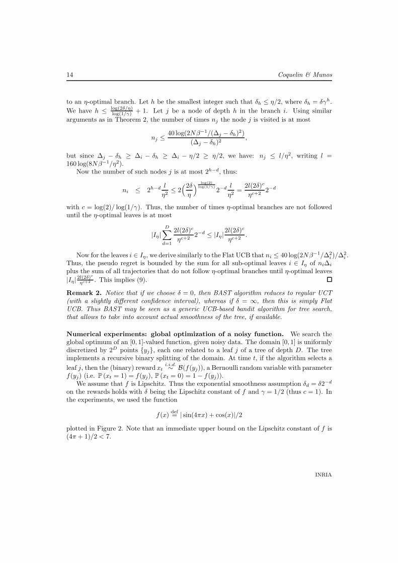
Figure 2: Function f rescaled (in plain) and proportion nj/n of leaves visitation for BASTwith δ = 7, depth D = 10, after n = 104 and n = 106 rounds.

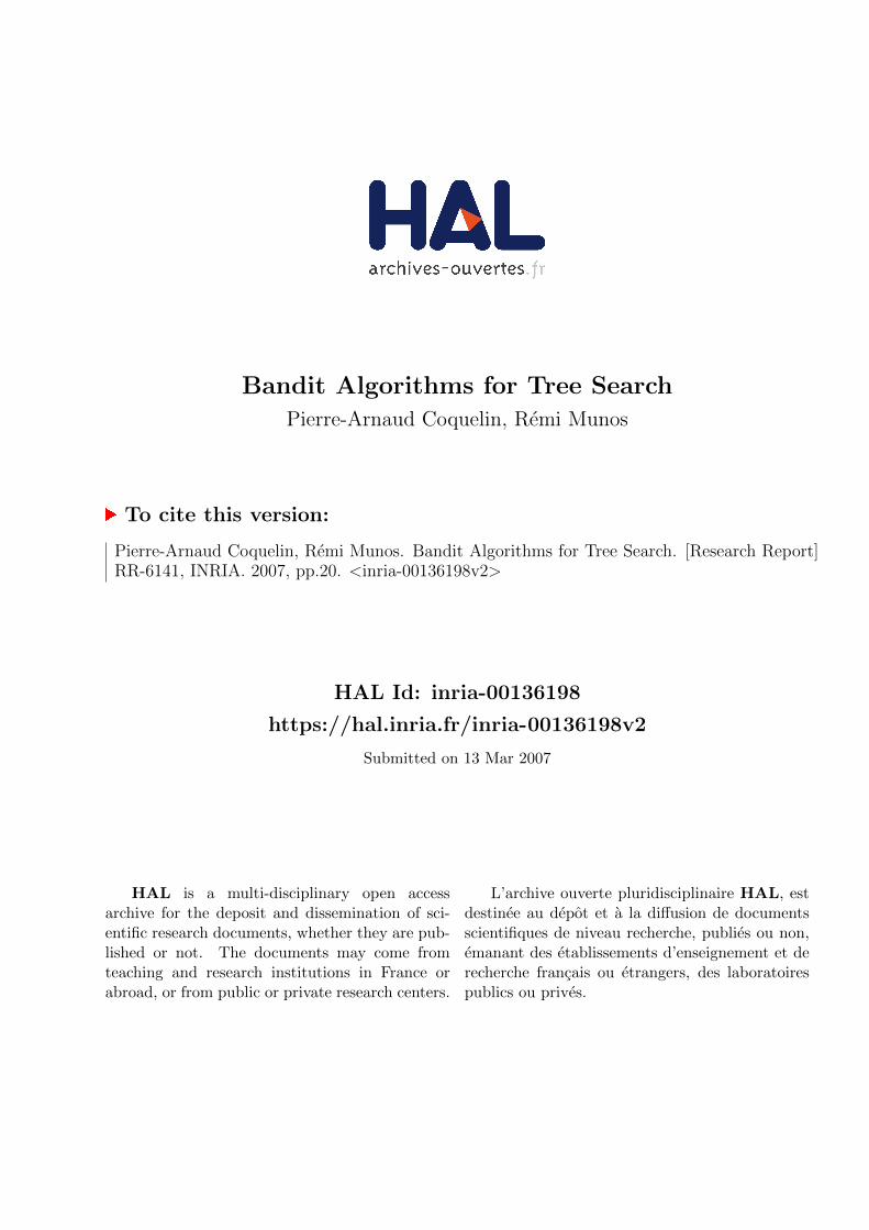
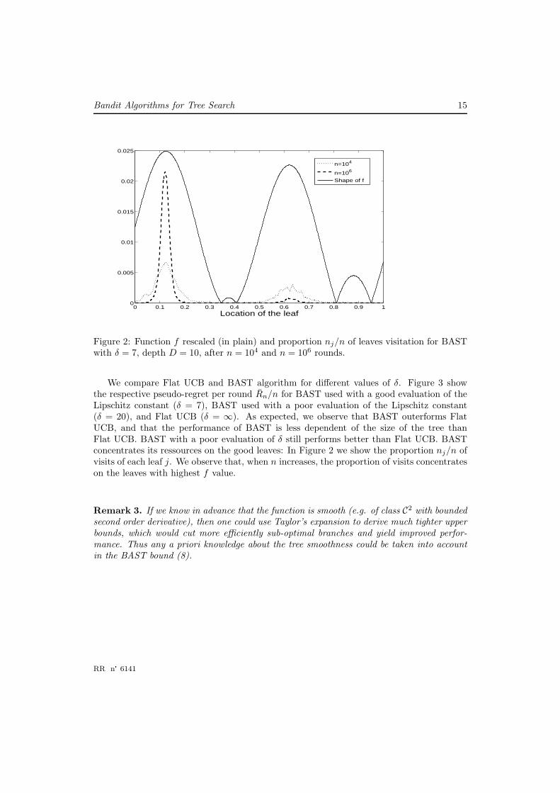
We compare Flat UCB and BAST algorithm for different values of δ. Figure 3 showthe respective pseudo-regret per round Rn/n for BAST used with a good evaluation of theLipschitz constant (δ = 7), BAST used with a poor evaluation of the Lipschitz constant(δ = 20), and Flat UCB (δ = ∞). As expected, we observe that BAST outerforms FlatUCB, and that the performance of BAST is less dependent of the size of the tree thanFlat UCB. BAST with a poor evaluation of δ still performs better than Flat UCB. BASTconcentrates its ressources on the good leaves: In Figure 2 we show the proportion nj/n ofvisits of each leaf j. We observe that, when n increases, the proportion of visits concentrateson the leaves with highest f value.

Remark 3. If we know in advance that the function is smooth (e.g. of class C2 with boundedsecond order derivative), then one could use Taylor’s expansion to derive much tighter upperbounds, which would cut more efficiently sub-optimal branches and yield improved perfor-mance. Thus any a priori knowledge about the tree smoothness could be taken into accountin the BAST bound (8).

RR n° 6141

16 Coquelin & Munos

5 10 15 200

0.05

0.1

0.15

0.2

0.25

0.3

0.35

0.4

Depth of the tree

Pseu

do re

gret

per r

ound

L=7L=20Flat

Figure 3: Pseudo regret per round Rn/n for n = 106, as a function of the depth D ∈5, 10, 15, 20, for BAST with δ ∈ 7, 20 and Flat UCB.

6 Growing trees

If the tree is too big (possibly infinite) to be represented, one may wish to discover ititeratively, exploring it as the same time as searching for an optimal value. We proposean incremental algorithm similar to the method described in [Cou06] and [GWMT06]: Thealgorithm starts with only the root node. Then, at each stage n it chooses which leaf, callit i, to expand next. Expanding a leaf means turning it into a node i, and adding in ourcurrent tree representation its children leaves i1 and i2, from which a reward (one for eachchild) is received. The process is then repeated in the new tree.

We make an assumption on the rewards: from any leaf j, the received reward x is arandom variable whose expected value satisfies: µj − E[x] ≤ δd, where d is the depth of j,and µj the value of j (defined as previously by the maximum of its children values).

Such an iterative growing tree requires a amount of memory O(n) directly related to thenumber of exploration rounds in the tree.

We now apply BAST algorithm and expect the tree to grow in an asymmetric way,expanding in depth the most promising branches first, leaving mainly unbuilt the sub-optimal branches.

Theorem 5. Consider this incremental tree method using Algorithm 1 defined by the bound(8) with the confidence interval

cni

def=

√

2 log(n(n + 1)ni(ni + 1)β−1)

ni,

INRIA


where n is the current number of expanded nodes. Then, with probability 1 − β, for anysub-optimal node i (of depth d), i.e. s.t. ∆i > 0,

ni ≤ 10(δ

c

)c(2 + c

∆i

)c+2

log(n(n + 1)

β

(2 + c)2

2∆2i

)

2−d. (10)

Thus this algorithm essentially develops the optimal branch, i.e. except for O(log(n))samples at each depth, all computational resources are devoted to further explore the optimalbranch.

Proof. Consider the event E under which |Xi,ni − Xi,ni | ≤ cni for all expanded nodes 1 ≤i ≤ n, all times ni ≥ 1, and all rounds n ≥ 1. The confidence interval cni are suchthat P (E) ≥ 1 − β. At round n, let i be a node of depth d. Let h be a depth such

that δh < ∆i. This is satisfied for all integer h ≥ log(δ/∆i)log(1/γ) . Similarly to Flat UCB, we

deduce that the number of times nj a node j of depth h has been visited is bounded by40 log(2n(n + 1)β−1/(∆i − δh)2)/(∆i − δh)2. Thus i has been visited at most

ni ≤ minh≥

log(δ/∆i)

log(1/γ)

2h−d 40 log(2n(n + 1)β−1/(∆i − δh)2)

(∆i − δh)2.

This function is minimized (neglecting the log term) for h = log( δ(2+c)c∆i

)/ log(1/γ), whichleads to (10).

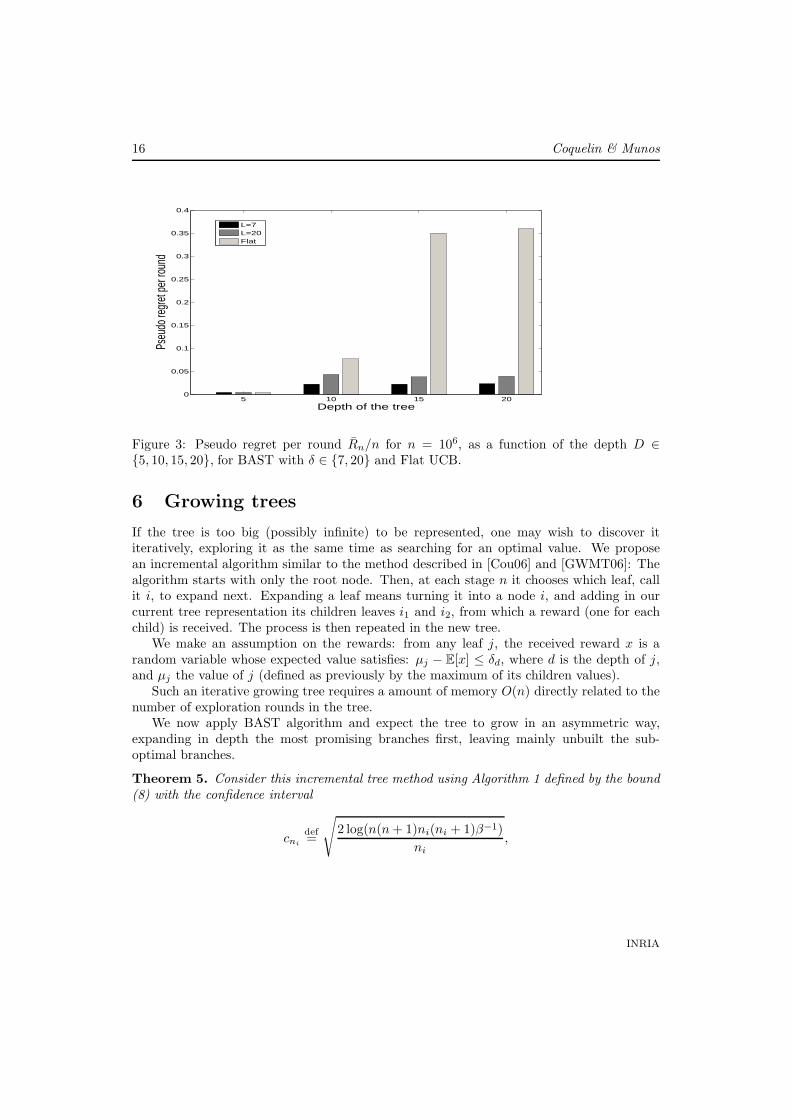
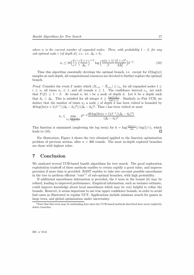
For illustration, Figure 4 shows the tree obtained applied to the function optimizationproblem of previous section, after n = 300 rounds. The most in-depth explored branchesare those with highest value.

7 Conclusion

We analyzed several UCB-based bandit algorithms for tree search. The good explorationexploitation tradeoff of these methods enables to return rapidly a good value, and improveprecision if more time is provided. BAST enables to take into account possible smoothnessin the tree to perform efficient “cuts”1 of sub-optimal branches, with high probability.

If additional smoothness information is provided, the δ term in the bound (8) may berefined, leading to improved performance. Empirical information, such as variance estimate,could improve knowledge about local smoothness which may be very helpful to refine thebounds. However, it seems important to use true upper confidence bounds, in order to avoidbad cases as illustrated in regular UCT. Applications include minimax search for games inlarge trees, and global optimization under uncertainty.

1Note that this term may be misleading here since the UCB-based methods described here never explicitly

delete branches

RR n° 6141

18 Coquelin & Munos

Figure 4: Tree resulting from the iterative growing BAST algorithm, after n = 300 rounds,with δ = 7.

INRIA


Acknowledgements

We wish to thank Jean-Francois Hren for running the numerical experiments.

References

[ACBF02] P. Auer, N. Cesa-Bianchi, and P. Fischer. Finite-time analysis of the multiarmed banditproblem. Machine Learning Journal, 47(2-3):235–256, 2002.

[Cou06] R. Coulom. Efficient selectivity and backup operators in Monte-Carlo tree search. 5th

International Conference on Computer and Games, 2006.

[GDL96] L. Gyorfi, L. Devroye, and G. Lugosi. A Probabilistic Theory of Pattern Recognition.Springer-Verlag, 1996.

[GWMT06] S. Gelly, Y. Wang, R. Munos, and O. Teytaud. Modication of UCT with patterns inMonte-Carlo go. Technical Report INRIA RR-6062, 2006.

[KS06] L. Kocsis and Cs. Szepesvari. Bandit based monte-carlo planning. European Conference

on Machine Learning, pages 282–293, 2006.

RR n° 6141

Unité de recherche INRIA FutursParc Club Orsay Université - ZAC des Vignes

4, rue Jacques Monod - 91893 ORSAY Cedex (France)

Unité de recherche INRIA Lorraine : LORIA, Technopôle de Nancy-Brabois - Campus scientifique615, rue du Jardin Botanique - BP 101 - 54602 Villers-lès-Nancy Cedex (France)

Unité de recherche INRIA Rennes : IRISA, Campus universitaire de Beaulieu - 35042 Rennes Cedex (France)Unité de recherche INRIA Rhône-Alpes : 655, avenue de l’Europe - 38334 Montbonnot Saint-Ismier (France)

Unité de recherche INRIA Rocquencourt : Domaine de Voluceau- Rocquencourt - BP 105 - 78153 Le Chesnay Cedex (France)Unité de recherche INRIA Sophia Antipolis : 2004, route des Lucioles - BP 93 - 06902 Sophia Antipolis Cedex (France)

ÉditeurINRIA - Domaine de Voluceau - Rocquencourt, BP 105 - 78153 Le Chesnay Cedex (France)http://www.inria.fr

ISSN 0249-6399

Bandit Algorithms for Tree Search

Documents

Transcript of Bandit Algorithms for Tree Search