PPA-based methods for monotone inverse variational inequalities
Upload
khangminh22Category
view
5download
0
.
.
.
.
.
.
.
.
.
.
.
.
.
.
.
.
.
.
.
.
.
.
.
.
.
.
.
.
.
.
.
.
.
.
.
.
.
.
.
.
Tree-Based Methods
Chapter 8
Chapter 8 1 / 55
.
.
.
.
.
.
.
.
.
.
.
.
.
.
.
.
.
.
.
.
.
.
.
.
.
.
.
.
.
.
.
.
.
.
.
.
.
.
.
.
1 8.1 The basics of decision trees.
2 8.2 Bagging, random forests and boosting
Chapter 8 2 / 55

.
.
.
.
.
.
.
.
.
.
.
.
.
.
.
.
.
.
.
.
.
.
.
.
.
.
.
.
.
.
.
.
.
.
.
.
.
.
.
.
About this chapter
• Decisions trees: splitting each variable sequentially, creatingrectugular regions.
• Making fitting/prediction locally at each region.
• It is intuitive and easy to implement, may have good interpreation.
• Generally of lower prediction accuracy.
• Bagging, random forests and boosting ... make fitting/predictionbased on a number of trees.
• Bagging and Boosting are general methodologies, not just limitedto trees.
Chapter 8 3 / 55

.
.
.
.
.
.
.
.
.
.
.
.
.
.
.
.
.
.
.
.
.
.
.
.
.
.
.
.
.
.
.
.
.
.
.
.
.
.
.
.
8.1 The basics of decision trees.
Regression trees
• Trees can be applied to both regression and classifcation.
• CART refers to classification and regression trees.
• We first consider regression trees through an example of predictingBaseball players’ salaries.
Chapter 8 4 / 55

.
.
.
.
.
.
.
.
.
.
.
.
.
.
.
.
.
.
.
.
.
.
.
.
.
.
.
.
.
.
.
.
.
.
.
.
.
.
.
.
8.1 The basics of decision trees.
The Hitters data
• Response/outputs: Salary.
• Covarites/Inputs:Years (the number of years that he has played in the majorleagues)Hits (the number of hits that he made in the previous year).
• preparing data: remove the observations with missing data andlog-transformed the Salary (preventing heavy right-skewness)
Chapter 8 5 / 55
.
.
.
.
.
.
.
.
.
.
.
.
.
.
.
.
.
.
.
.
.
.
.
.
.
.
.
.
.
.
.
.
.
.
.
.
.
.
.
.
8.1 The basics of decision trees.
|Years < 4.5
Hits < 117.5
5.11
6.00 6.74
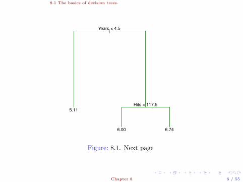
Figure: 8.1. Next page
Chapter 8 6 / 55

.
.
.
.
.
.
.
.
.
.
.
.
.
.
.
.
.
.
.
.
.
.
.
.
.
.
.
.
.
.
.
.
.
.
.
.
.
.
.
.
8.1 The basics of decision trees.
Figure 8.1. For the Hitters data, a regression tree for predicting the logsalary of a baseball player, based on the number of years that he hasplayed in the major leagues and the number of hits that he made in theprevious year. At a given internal node, the label (of the form Xj < tk)indicates the left-hand branch emanating from that split, and theright-hand branch corresponds to Xj ≥ tk. For instance, the split atthe top of the tree results in two large branches. The left-hand branchcorresponds to Years< 4.5, and the right-hand branch corresponds toYears≥ 4.5. The tree has two internal nodes and three terminal nodes,or leaves. The number in each leaf is the mean of the response for theobservations that fall there.
Chapter 8 7 / 55
.
.
.
.
.
.
.
.
.
.
.
.
.
.
.
.
.
.
.
.
.
.
.
.
.
.
.
.
.
.
.
.
.
.
.
.
.
.
.
.
8.1 The basics of decision trees.
Years
Hits
1
117.5
238
1 4.5 24
R1
R3
R2
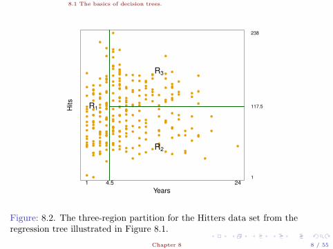
Figure: 8.2. The three-region partition for the Hitters data set from theregression tree illustrated in Figure 8.1.
Chapter 8 8 / 55
.
.
.
.
.
.
.
.
.
.
.
.
.
.
.
.
.
.
.
.
.
.
.
.
.
.
.
.
.
.
.
.
.
.
.
.
.
.
.
.
8.1 The basics of decision trees.
Estimation/prediction
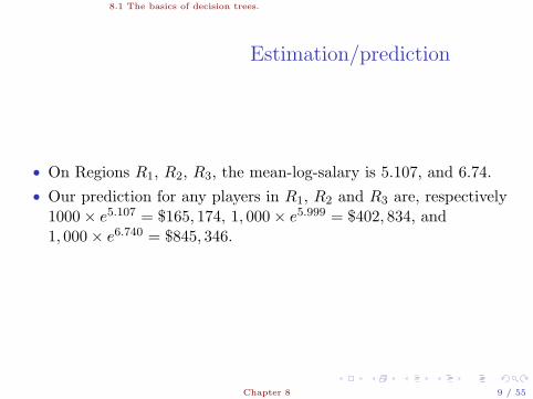
• On Regions R1, R2, R3, the mean-log-salary is 5.107, and 6.74.
• Our prediction for any players in R1, R2 and R3 are, respectively1000× e5.107 = $165, 174, 1, 000× e5.999 = $402, 834, and1, 000× e6.740 = $845, 346.
Chapter 8 9 / 55
.
.
.
.
.
.
.
.
.
.
.
.
.
.
.
.
.
.
.
.
.
.
.
.
.
.
.
.
.
.
.
.
.
.
.
.
.
.
.
.
8.1 The basics of decision trees.
Estimation/prediction
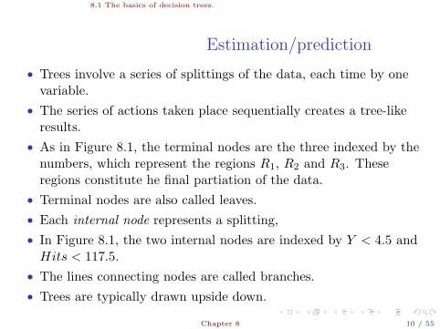
• Trees involve a series of splittings of the data, each time by onevariable.
• The series of actions taken place sequentially creates a tree-likeresults.
• As in Figure 8.1, the terminal nodes are the three indexed by thenumbers, which represent the regions R1, R2 and R3. Theseregions constitute he final partiation of the data.
• Terminal nodes are also called leaves.
• Each internal node represents a splitting,
• In Figure 8.1, the two internal nodes are indexed by Y < 4.5 andHits < 117.5.
• The lines connecting nodes are called branches.
• Trees are typically drawn upside down.
Chapter 8 10 / 55
.
.
.
.
.
.
.
.
.
.
.
.
.
.
.
.
.
.
.
.
.
.
.
.
.
.
.
.
.
.
.
.
.
.
.
.
.
.
.
.
8.1 The basics of decision trees.
Two step towards prediction
• Run the splitting according to input values sequentially, andobtain final partition of the data in regions R1, ..., RJ .
• For any new observation with covariates in region Rk, we predictits response by the average of the reponses of the data points inregion Rk.
Chapter 8 11 / 55
.
.
.
.
.
.
.
.
.
.
.
.
.
.
.
.
.
.
.
.
.
.
.
.
.
.
.
.
.
.
.
.
.
.
.
.
.
.
.
.
8.1 The basics of decision trees.
How to split
• Suppose we wish to partition a region R. In other words, we wishto separate the data in region R into two parts, day R1 and R2,according to one input values.
• What would be the optimal or efficient split in some sense?
• Only two flexibility in the split: 1. Choice of the input variable tosplit, 2. the cutpoint of the split of that chose input.
• Imagine that this is the final split of R: R1 and R2 would beleaves.And we would use the mean response of data in R1 and R2 topredict the response of any new/old observations.We wish our choice of R1 and R2 would be optimal in the sense ofachieving miminum prediction error on the training data in regionR.
Chapter 8 12 / 55
.
.
.
.
.
.
.
.
.
.
.
.
.
.
.
.
.
.
.
.
.
.
.
.
.
.
.
.
.
.
.
.
.
.
.
.
.
.
.
.
8.1 The basics of decision trees.
Recursive binary splitting
• A greedy algorithm (geedy means it is optimal at the current step):For j = 1, ..., p and all real value s, let R1(j, s) = {i ∈ R : Xj < s}and R2(j, s) = {i ∈ R : Xj ≥ s}. And let y1 and y2 be the meanresponse of all observations in R1(j, s) and R2(j, s), respectively.Consider the following prediction error:
RSSnew =∑
i∈R1(j,s)
(yi − y1)2 +
∑i∈R2(j,s)
(yi − y2)2
Choose the split which has the smallest prediction error. This splitis the optimal one, denoted as R1 and R2.
• Continue the split till the final partition.
Chapter 8 13 / 55

.
.
.
.
.
.
.
.
.
.
.
.
.
.
.
.
.
.
.
.
.
.
.
.
.
.
.
.
.
.
.
.
.
.
.
.
.
.
.
.
8.1 The basics of decision trees.
|
t1
t2
t3
t4
R1
R1
R2
R2
R3
R3
R4
R4
R5
R5
X1
X1X1
X2
X2
X2
X1 ≤ t1
X2 ≤ t2 X1 ≤ t3
X2 ≤ t4
Chapter 8 14 / 55
.
.
.
.
.
.
.
.
.
.
.
.
.
.
.
.
.
.
.
.
.
.
.
.
.
.
.
.
.
.
.
.
.
.
.
.
.
.
.
.
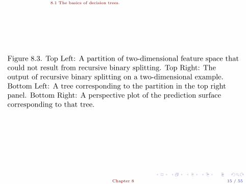
8.1 The basics of decision trees.
Figure 8.3. Top Left: A partition of two-dimensional feature space thatcould not result from recursive binary splitting. Top Right: Theoutput of recursive binary splitting on a two-dimensional example.Bottom Left: A tree corresponding to the partition in the top rightpanel. Bottom Right: A perspective plot of the prediction surfacecorresponding to that tree.
Chapter 8 15 / 55
.
.
.
.
.
.
.
.
.
.
.
.
.
.
.
.
.
.
.
.
.
.
.
.
.
.
.
.
.
.
.
.
.
.
.
.
.
.
.
.
8.1 The basics of decision trees.
When to stop split
• The problem of when to stop.
• If too many steps of splitting: many leaves, too complex model,small bias but large variance, may overfit.
• If too few steps of splitting: few leaves, too simple model, largebias but small variance, may underfit.
Chapter 8 16 / 55

.
.
.
.
.
.
.
.
.
.
.
.
.
.
.
.
.
.
.
.
.
.
.
.
.
.
.
.
.
.
.
.
.
.
.
.
.
.
.
.
8.1 The basics of decision trees.
One natural idea
• When splitting R into R1 and R2, consider the RSS before the split
RSSold =∑i∈R
(yi − y)2
where y is the average of the response of data in R. With theoptimal split, the reduction of RSS is
RSSold − RSSnew
• We can pre-choose a threshold, h, and decide the worthiness of thesplit.
• If the reduction is smaller than h, we do not do it, and stop rightthere; then R is one terminal node (a leave).
• If the reduction is greater than h, we make the split, and continuewith next step.
Chapter 8 17 / 55

.
.
.
.
.
.
.
.
.
.
.
.
.
.
.
.
.
.
.
.
.
.
.
.
.
.
.
.
.
.
.
.
.
.
.
.
.
.
.
.
8.1 The basics of decision trees.
One natural idea
• The idea is seemingly reasonable, but is too near-sighted.
• Only look at the effect of the current split.
• It is possible that even if the current split is not effective, thefuture splits could be effective and, maybe, very effective.
Chapter 8 18 / 55

.
.
.
.
.
.
.
.
.
.
.
.
.
.
.
.
.
.
.
.
.
.
.
.
.
.
.
.
.
.
.
.
.
.
.
.
.
.
.
.
8.1 The basics of decision trees.
Tree pruning
• Grow a very large tree.
• Prune the true back to obtain a subtree.
• Objective: find the subtree that has the best test error.
• Cannot use cross-validation to examine the test errors for allpossible subtrees, since there are just too many.
• Even if we can, this would probably be overfitting, since modelspace is too large.
Chapter 8 19 / 55
.
.
.
.
.
.
.
.
.
.
.
.
.
.
.
.
.
.
.
.
.
.
.
.
.
.
.
.
.
.
.
.
.
.
.
.
.
.
.
.
8.1 The basics of decision trees.
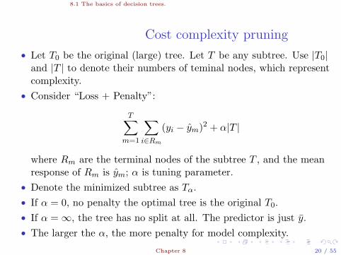
Cost complexity pruning
• Let T0 be the original (large) tree. Let T be any subtree. Use |T0|and |T | to denote their numbers of teminal nodes, which representcomplexity.
• Consider “Loss + Penalty”:
T∑m=1
∑i∈Rm
(yi − ym)2 + α|T |
where Rm are the terminal nodes of the subtree T , and the meanresponse of Rm is ym; α is tuning parameter.
• Denote the minimized subtree as Tα.
• If α = 0, no penalty the optimal tree is the original T0.
• If α =∞, the tree has no split at all. The predictor is just y.
• The larger the α, the more penalty for model complexity.
Chapter 8 20 / 55
.
.
.
.
.
.
.
.
.
.
.
.
.
.
.
.
.
.
.
.
.
.
.
.
.
.
.
.
.
.
.
.
.
.
.
.
.
.
.
.
8.1 The basics of decision trees.
Cost complexity pruning
• Just like Lasso, there exists efficient computation algorithm tocompute the entire sequence of Tα for all α.
• Use cross-validation to find the best α to minimize the test error.
Chapter 8 21 / 55
.
.
.
.
.
.
.
.
.
.
.
.
.
.
.
.
.
.
.
.
.
.
.
.
.
.
.
.
.
.
.
.
.
.
.
.
.
.
.
.
8.1 The basics of decision trees.
The algorithm
• 1. Use recursive binary splitting to grow a large tree on thetraining data, stopping only when each terminal node has fewerthan some minimum number of observations.
• 2. Apply cost complexity pruning to the large tree in order toobtain a sequence of best subtrees, as a function of α.
Chapter 8 22 / 55
.
.
.
.
.
.
.
.
.
.
.
.
.
.
.
.
.
.
.
.
.
.
.
.
.
.
.
.
.
.
.
.
.
.
.
.
.
.
.
.
8.1 The basics of decision trees.
The algorithm
• 3. Use K-fold cross-validation to determine best α. That is, dividethe training observations into K folds. For each k = 1, ...,K(a) Repeat Steps 1 and 2 on all but the kth fold of the trainingdata.(b) Evaluate the mean squared prediction error on the data in theleft-out k-th fold, as a function of α.(c) Average the results for each value of α, and pick α to minimizethe average error.
• 4. Return the subtree from Step 2 that corresponds to the chosenvalue of α.
Chapter 8 23 / 55

.
.
.
.
.
.
.
.
.
.
.
.
.
.
.
.
.
.
.
.
.
.
.
.
.
.
.
.
.
.
.
.
.
.
.
.
.
.
.
.
8.1 The basics of decision trees.
|Years < 4.5
RBI < 60.5
Putouts < 82
Years < 3.5
Years < 3.5
Hits < 117.5
Walks < 43.5
Runs < 47.5
Walks < 52.5
RBI < 80.5
Years < 6.5
5.487
4.622 5.183
5.394 6.189
6.015 5.5716.407 6.549
6.459 7.0077.289
Figure: 8.4. Regression tree analysis for the Hitters data. The unpruned treethat results from top-down greedy splitting on the training data is shown.
Chapter 8 24 / 55
.
.
.
.
.
.
.
.
.
.
.
.
.
.
.
.
.
.
.
.
.
.
.
.
.
.
.
.
.
.
.
.
.
.
.
.
.
.
.
.
8.1 The basics of decision trees.
2 4 6 8 10
0.0
0.2
0.4
0.6
0.8
1.0
Tree Size
Me
an
Sq
ua
red
Err
or
Training
Cross−Validation
Test
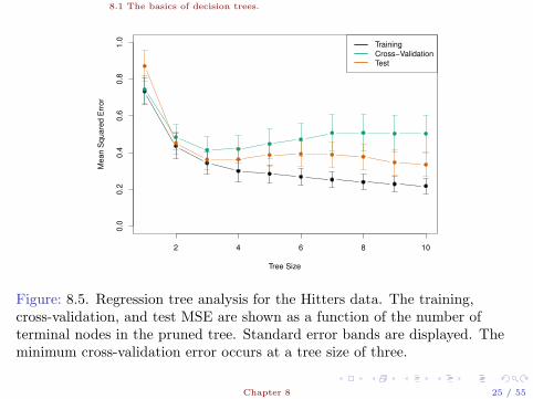
Figure: 8.5. Regression tree analysis for the Hitters data. The training,cross-validation, and test MSE are shown as a function of the number ofterminal nodes in the pruned tree. Standard error bands are displayed. Theminimum cross-validation error occurs at a tree size of three.
Chapter 8 25 / 55
.
.
.
.
.
.
.
.
.
.
.
.
.
.
.
.
.
.
.
.
.
.
.
.
.
.
.
.
.
.
.
.
.
.
.
.
.
.
.
.
8.1 The basics of decision trees.
Classification trees
• Regression has numerical responses; and classification hasqualitative responses.
• Recall that for regression trees, we chose to obtain the greatestreduction of RSS.RSS is using sum of squares to measure the error.
• For classification trees, one can follow the same line of procedureas that of regression trees, but using error measurements that aremore appropriate for classification.
Chapter 8 26 / 55
.
.
.
.
.
.
.
.
.
.
.
.
.
.
.
.
.
.
.
.
.
.
.
.
.
.
.
.
.
.
.
.
.
.
.
.
.
.
.
.
8.1 The basics of decision trees.
Classification error rates
• For a region R, let pk be the percentage of observations in thisregion that belong to class k.
• We assign any new observation in region R as from the class withlargest pk, which is the so-called most commonly occuring class intraining data.
Chapter 8 27 / 55

.
.
.
.
.
.
.
.
.
.
.
.
.
.
.
.
.
.
.
.
.
.
.
.
.
.
.
.
.
.
.
.
.
.
.
.
.
.
.
.
8.1 The basics of decision trees.
The impurity measure
• The classification error rate (for this region R) is
E = 1−maxkpk.
• The Gini index is
G =
K∑k=1
pk(1− pk)
• The cross-entropy is
D = −K∑k=1
pk log(pk)
.
Chapter 8 28 / 55

.
.
.
.
.
.
.
.
.
.
.
.
.
.
.
.
.
.
.
.
.
.
.
.
.
.
.
.
.
.
.
.
.
.
.
.
.
.
.
.
8.1 The basics of decision trees.
• If R is nearly pure, most of the observations are from one class,then the Gini-index and cross-entropy would take smaller valuesthan classfication error rate.
• Gini-index and cross-entropy are more sentive to node purity.
• To evaluate the quality of a particluar split, the Gini-index andcross-entropy are more popularly used as error measurementcrietria than classification error rate.
• Any of these three approaches might be used when pruning thetree.
• The classification error rate is preferable if prediction accuracy ofthe final pruned tree is the goal.
Chapter 8 29 / 55
.
.
.
.
.
.
.
.
.
.
.
.
.
.
.
.
.
.
.
.
.
.
.
.
.
.
.
.
.
.
.
.
.
.
.
.
.
.
.
.
8.1 The basics of decision trees.
|Thal:a
Ca < 0.5
MaxHR < 161.5
RestBP < 157
Chol < 244MaxHR < 156
MaxHR < 145.5
ChestPain:bc
Chol < 244 Sex < 0.5
Ca < 0.5
Slope < 1.5
Age < 52 Thal:b
ChestPain:a
Oldpeak < 1.1
RestECG < 1
No YesNo
NoYes
No
No No No Yes
Yes No No
No Yes
Yes Yes
Yes
5 10 15
0.0
0.1
0.2
0.3
0.4
0.5
0.6
Tree Size
Err
or
TrainingCross−ValidationTest
|Thal:a
Ca < 0.5
MaxHR < 161.5 ChestPain:bc
Ca < 0.5
No No
No Yes
Yes Yes
Chapter 8 30 / 55

.
.
.
.
.
.
.
.
.
.
.
.
.
.
.
.
.
.
.
.
.
.
.
.
.
.
.
.
.
.
.
.
.
.
.
.
.
.
.
.
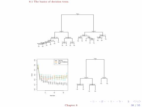
8.1 The basics of decision trees.
Figure 8.6. Heart data. Top: The unpruned tree. Bottom Left:Cross-validation error, training, and test error, for different sizes of thepruned tree. Bottom Right: The pruned tree corresponding to theminimal cross-validation error.
Chapter 8 31 / 55

.
.
.
.
.
.
.
.
.
.
.
.
.
.
.
.
.
.
.
.
.
.
.
.
.
.
.
.
.
.
.
.
.
.
.
.
.
.
.
.
8.1 The basics of decision trees.
Trees vs. Linear models
• For regression model:Y = f(X) + ϵ
• Linear model assumes
f(X) = β0 +
p∑j=1
Xjβj
• Regression trees assume
f(X) =
M∑j=1
cm1(X ∈ Rm)
where R1, ..., RM are rectagular partitions of the input space.
• If the underlying realation is close to linear, linear model is better.Otherwise, regression trees are generally better. (Uselesscomments)
Chapter 8 32 / 55
.
.
.
.
.
.
.
.
.
.
.
.
.
.
.
.
.
.
.
.
.
.
.
.
.
.
.
.
.
.
.
.
.
.
.
.
.
.
.
.
8.1 The basics of decision trees.
−2 −1 0 1 2
−2
−1
01
2
X1
X2
−2 −1 0 1 2
−2
−1
01
2
X1
X2
−2 −1 0 1 2
−2
−1
01
2
X1
X2
−2 −1 0 1 2
−2
−1
01
2
X1
X2
Chapter 8 33 / 55
.
.
.
.
.
.
.
.
.
.
.
.
.
.
.
.
.
.
.
.
.
.
.
.
.
.
.
.
.
.
.
.
.
.
.
.
.
.
.
.
8.1 The basics of decision trees.
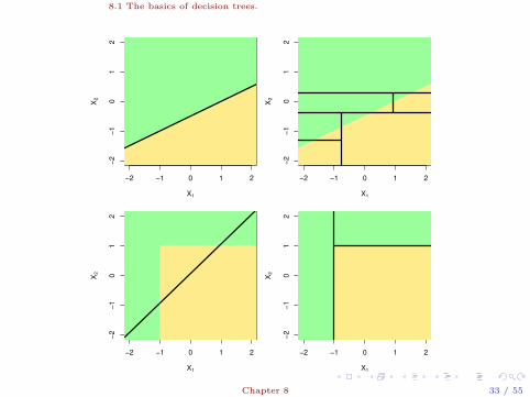
Figure 8.7. Top Row: A two-dimensional classification example inwhich the true decision boundary is linear, and is indicated by theshaded regions. A classical approach that assumes a linear boundary(left) will outperform a decision tree that performs splits parallel to theaxes (right). Bottom Row: Here the true decision boundary isnon-linear. Here a linear model is unable to capture the true decisionboundary (left), whereas a decision tree is successful (right).
Chapter 8 34 / 55
.
.
.
.
.
.
.
.
.
.
.
.
.
.
.
.
.
.
.
.
.
.
.
.
.
.
.
.
.
.
.
.
.
.
.
.
.
.
.
.
8.1 The basics of decision trees.
Advantages of Trees
• Trees are very easy to explain to people. In fact, they are eveneasier to explain than linear regression!
• Some people believe that decision trees more closely mirror humandecision-making than do the regression and classificationapproaches seen in previous chapters.
• Trees can be displayed graphically, and are easily interpreted evenby a non-expert (especially if they are small).
• Trees can easily handle qualitative predictors without the need tocreate dummy variables.
Chapter 8 35 / 55
.
.
.
.
.
.
.
.
.
.
.
.
.
.
.
.
.
.
.
.
.
.
.
.
.
.
.
.
.
.
.
.
.
.
.
.
.
.
.
.
8.1 The basics of decision trees.
Disadvantages of Trees
• Trees generally do not have the same level of predictive accuracyas some of the other regression and classification approaches seenin this book.
• Trees can be very non-robust. In other words, a small change inthe data can cause a large change in the final estimated tree.
• However, by aggregating many decision trees, using methods likebagging, random forests, and boosting, the predictive performanceof trees can be substantially improved. We introduce theseconcepts in the next section.
Chapter 8 36 / 55

.
.
.
.
.
.
.
.
.
.
.
.
.
.
.
.
.
.
.
.
.
.
.
.
.
.
.
.
.
.
.
.
.
.
.
.
.
.
.
.
8.2 Bagging, random forests and boosting
Bagging (Boostrap Aggregating)
• A general purpose procedure to reduce variance of a learningmethod.
• A model averaging technique.
• Decision tree is generally a high variance method. (Apply themethod based on different data based on same sampling schemewould lead to very different result.)
• Average of iid random variables would have a reduced varianceσ2/n
Chapter 8 37 / 55
.
.
.
.
.
.
.
.
.
.
.
.
.
.
.
.
.
.
.
.
.
.
.
.
.
.
.
.
.
.
.
.
.
.
.
.
.
.
.
.
8.2 Bagging, random forests and boosting
The procedure.
• Modelyi = f(xi) + ϵi, i = 1, ..., n.
• Suppose a statistical learning method gives f(·) based on thetraining data (yi, xi), i =, 1..., n.
• For example,
1 Linear model: f(x) = β0 + βTxi
2 KNN: f(x) =∑J
j=1 yRjwith least distance to K-cluster partition.
3 Decision tree: f(x) =∑J
j=1 yRjwith rectangular partition.
4 ...
Chapter 8 38 / 55
.
.
.
.
.
.
.
.
.
.
.
.
.
.
.
.
.
.
.
.
.
.
.
.
.
.
.
.
.
.
.
.
.
.
.
.
.
.
.
.
8.2 Bagging, random forests and boosting
The procedure of Bagging
• Data (yi, xi), i = 1, ..., n; and a learning method f
• Draw a boostrap sample from the data, and compute a f∗1 based
on this set of bootstrap sample.
• Draw another boostrap sample from the data, and compute a f∗2
based on this set of bootstrap sample.
• ....
• Repeat M times, obtain f∗1 , ...., f
∗M .
• Produce the learning method with bagging as
1
M
M∑j=1
f∗j
Chapter 8 39 / 55
.
.
.
.
.
.
.
.
.
.
.
.
.
.
.
.
.
.
.
.
.
.
.
.
.
.
.
.
.
.
.
.
.
.
.
.
.
.
.
.
8.2 Bagging, random forests and boosting
The Bagging
• Bagging is general-purpose.
• It works best for high variance low bias learning methods.
• This is the case for decision trees, particularly deep trees.
• Also the case for large p.
• If the response is qualitative, we can take the majority vote (notaveraging) of the predicted class based on all learning methodsbased on boostrap samples.
Chapter 8 40 / 55
.
.
.
.
.
.
.
.
.
.
.
.
.
.
.
.
.
.
.
.
.
.
.
.
.
.
.
.
.
.
.
.
.
.
.
.
.
.
.
.
8.2 Bagging, random forests and boosting
0 50 100 150 200 250 300
0.1
00
.15
0.2
00
.25
0.3
0
Number of Trees
Err
or
Test: Bagging
Test: RandomForest
OOB: Bagging
OOB: RandomForest
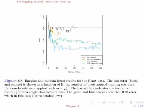
Figure: 8.8. Bagging and random forest results for the Heart data. The test error (blackand orange) is shown as a function of B, the number of bootstrapped training sets used.Random forests were applied with m =
√p. The dashed line indicates the test error
resulting from a single classification tree. The green and blue traces show the OOB error,which in this case is considerably lower
Chapter 8 41 / 55

.
.
.
.
.
.
.
.
.
.
.
.
.
.
.
.
.
.
.
.
.
.
.
.
.
.
.
.
.
.
.
.
.
.
.
.
.
.
.
.
8.2 Bagging, random forests and boosting
Out-of-Bag (OOB) error estimation
• Estimation of test error for the bagged model.
• For each bootstrap sample, observation i is bootstrap sampledwith probabilty (1− 1/n)n ≈ 1/e.
• For each bootstrap sample, the number of observations not takeninto this bootstrap sample is n(1− 1/n)n ≈ n/e. These arereferred to as out-of-bag (OOB) observations.
• For totally B bootstrap samples, about B/e times, the bootstrapsample does not contain observation i.
• The trees based on these bootstrap sample can be used to predictthe response of observation i. Tatoally about B/e predictions.
• We average these predictions (for regression) or take majority vote(for classification) to produce the Bagged prediction forobservation i, denote it as f∗(xi).
Chapter 8 42 / 55
.
.
.
.
.
.
.
.
.
.
.
.
.
.
.
.
.
.
.
.
.
.
.
.
.
.
.
.
.
.
.
.
.
.
.
.
.
.
.
.
8.2 Bagging, random forests and boosting
Out-of-Bag (OOB) error estimation
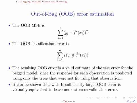
• The OOB MSE isn∑
i=1
(yi − f∗(xi))2
• The OOB classification error is
n∑i=1
I(yi /∈ f∗(xi))
• The resulting OOB error is a valid estimate of the test error for thebagged model, since the response for each observation is predictedusing only the trees that were not fit using that observation.
• It can be shown that with B sufficiently large, OOB error isvirtually equivalent to leave-one-out cross-validation error.
Chapter 8 43 / 55

.
.
.
.
.
.
.
.
.
.
.
.
.
.
.
.
.
.
.
.
.
.
.
.
.
.
.
.
.
.
.
.
.
.
.
.
.
.
.
.
8.2 Bagging, random forests and boosting
Variable importance measures
• Bagging improves prediction accuracy at the expense ofinterpretability.
• An overall summary of the importance of each predictor using theRSS (for bagging regression trees) or the Gini index (for baggingclassification trees).
• Bagging regression trees, we can record the total amount that theRSS is decreased due to splits over a given predictor, averagedover all B trees.
• A large value indicates an important predictor.
• Bagging classification trees, we can add up the total amount thatthe Gini index is decreased by splits over a given predictor,averaged over all B trees.
Chapter 8 44 / 55

.
.
.
.
.
.
.
.
.
.
.
.
.
.
.
.
.
.
.
.
.
.
.
.
.
.
.
.
.
.
.
.
.
.
.
.
.
.
.
.
8.2 Bagging, random forests and boosting
Thal
Ca
ChestPain
Oldpeak
MaxHR
RestBP
Age
Chol
Slope
Sex
ExAng
RestECG
Fbs
0 20 40 60 80 100
Variable Importance
Figure: 8.9. A variable importance plot for the Heart data. Variable importance iscomputed using the mean decrease in Gini index, and expressed relative to the maximum.
Chapter 8 45 / 55
.
.
.
.
.
.
.
.
.
.
.
.
.
.
.
.
.
.
.
.
.
.
.
.
.
.
.
.
.
.
.
.
.
.
.
.
.
.
.
.
8.2 Bagging, random forests and boosting
Random forest
• Same as bagging decision trees, except ...
• When building these decision trees, each time a split in a tree isconsidered, a random sample of m predictors is chosen as splitcandidates from the full set of p predictors
• Typically m ≈ √p.
Chapter 8 46 / 55
.
.
.
.
.
.
.
.
.
.
.
.
.
.
.
.
.
.
.
.
.
.
.
.
.
.
.
.
.
.
.
.
.
.
.
.
.
.
.
.
8.2 Bagging, random forests and boosting
Random forest
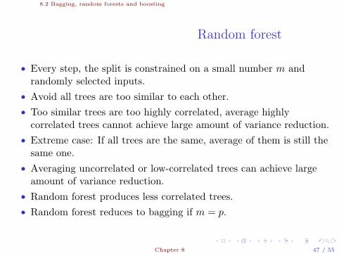
• Every step, the split is constrained on a small number m andrandomly selected inputs.
• Avoid all trees are too similar to each other.
• Too similar trees are too highly correlated, average highlycorrelated trees cannot achieve large amount of variance reduction.
• Extreme case: If all trees are the same, average of them is still thesame one.
• Averaging uncorrelated or low-correlated trees can achieve largeamount of variance reduction.
• Random forest produces less correlated trees.
• Random forest reduces to bagging if m = p.
Chapter 8 47 / 55

.
.
.
.
.
.
.
.
.
.
.
.
.
.
.
.
.
.
.
.
.
.
.
.
.
.
.
.
.
.
.
.
.
.
.
.
.
.
.
.
8.2 Bagging, random forests and boosting
0 100 200 300 400 500
0.2
0.3
0.4
0.5
Number of Trees
Te
st
Cla
ssific
atio
n E
rro
r
m=p
m=p/2
m= p
Figure: 8.10. Results from random forests for the 15-class gene expression data set withp = 500 predictors. The test error is displayed as a function of the number of trees. Eachcolored line corresponds to a different value of m, the number of predictors available forsplitting at each interior tree node. Random forests (m < p) lead to a slight improvementover bagging (m = p). A single classification tree has an error rate of 45.7%.
Chapter 8 48 / 55

.
.
.
.
.
.
.
.
.
.
.
.
.
.
.
.
.
.
.
.
.
.
.
.
.
.
.
.
.
.
.
.
.
.
.
.
.
.
.
.
8.2 Bagging, random forests and boosting
Boosting
• General purpose for improving learning methods by combiningmany weaker learners in attempt to produce a strong learner.
• Like bagging, boosting involves combining a large number ofweaker learners.
• The weaker learners are created sequentially. (no boostrapinvolved).
• Bagging create large variance and possibly over-fit boostraplearners and try to reduce their variance by averaging.
• Boosting create weak learners sequentially and slowly (to avoidover-fit).
Chapter 8 49 / 55

.
.
.
.
.
.
.
.
.
.
.
.
.
.
.
.
.
.
.
.
.
.
.
.
.
.
.
.
.
.
.
.
.
.
.
.
.
.
.
.
8.2 Bagging, random forests and boosting
Boosting
• Suppose we have model
yi = f(xi) + ϵi
and a learning method to produce f based on (yi, xi), i = 1, .., n.
• Start with an initial predictor f = 0. Let ri = yi.
• Start loop:
1 Fit the data (xi, ri), i = 1, .., n, to produce g.
2 Update f by f + λg.3 Update ri by ri − λg(xi).
• Continue the loop ... till a stop.
• Output f
• Note that the output f is the sum of λg at each step.
Chapter 8 50 / 55
.
.
.
.
.
.
.
.
.
.
.
.
.
.
.
.
.
.
.
.
.
.
.
.
.
.
.
.
.
.
.
.
.
.
.
.
.
.
.
.
8.2 Bagging, random forests and boosting
Algorithm for tree boosting
• 1. Set f(x) = 0 and ri = yi for all i in the training set.
• 2. For b = 1, 2, ..., B, repeat:1 Fit a tree with d splits (d+ 1 terminal nodes) to the training data
(xi, ri).
2 Update f by adding in a shrunken version of the new tree:
f(x)← f(x) + λfb(x)
3 Update the residuals,
ri ← ri − λfb(xi) = yi − f(xi).
• 3. Output the boosted model f . In fact,
f(x) =
B∑i=1
λf b(x).
Chapter 8 51 / 55
.
.
.
.
.
.
.
.
.
.
.
.
.
.
.
.
.
.
.
.
.
.
.
.
.
.
.
.
.
.
.
.
.
.
.
.
.
.
.
.
8.2 Bagging, random forests and boosting
Tuning parameters for boosting trees
• The number of trees B. Large B leads to overfit. (not a tuningparameter for bagging)
• The learning rate λ.
• The number d in splits in each tree (the size of each tree). Oftend = 1 works well, in which case each tree is a stump, consisting ofa single split
Chapter 8 52 / 55
.
.
.
.
.
.
.
.
.
.
.
.
.
.
.
.
.
.
.
.
.
.
.
.
.
.
.
.
.
.
.
.
.
.
.
.
.
.
.
.
8.2 Bagging, random forests and boosting
0 1000 2000 3000 4000 5000
0.0
50.1
00.1
50.2
00.2
5
Number of Trees
Test C
lassific
ation E
rror
Boosting: depth=1
Boosting: depth=2
RandomForest: m= p
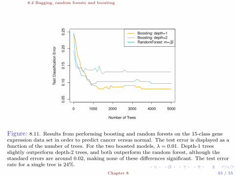
Figure: 8.11. Results from performing boosting and random forests on the 15-class geneexpression data set in order to predict cancer versus normal. The test error is displayed as afunction of the number of trees. For the two boosted models, λ = 0.01. Depth-1 treesslightly outperform depth-2 trees, and both outperform the random forest, although thestandard errors are around 0.02, making none of these differences significant. The test errorrate for a single tree is 24%.
Chapter 8 53 / 55

.
.
.
.
.
.
.
.
.
.
.
.
.
.
.
.
.
.
.
.
.
.
.
.
.
.
.
.
.
.
.
.
.
.
.
.
.
.
.
.
8.2 Bagging, random forests and boosting
Exercises
Run the R-Lab codes in Section *.3 of ISLRExercises 1-4 and 7-8 of Section 8.4 of ISLR
Chapter 8 54 / 55

.
.
.
.
.
.
.
.
.
.
.
.
.
.
.
.
.
.
.
.
.
.
.
.
.
.
.
.
.
.
.
.
.
.
.
.
.
.
.
.
8.2 Bagging, random forests and boosting
End of Chapter 8.
Chapter 8 55 / 55
Copyright © 2022 FDOKUMEN