Incremental Tree-Based Missing Data

Imputation with Lexicographic Ordering

Claudio ConversanoDepartment of Economics

University of CassinoVia M. Mazzaroppi, I-03043 Cassino (FR), Italy

conversa@unina.it

Roberta SicilianoDepartment of Mathematics and Statistics

University Federico II of NaplesVia Cinthia, Monte Sant’Angelo, I-80126, Napoli, Italy

roberta@unina.it

October 2, 2003

Abstract. In the framework of data imputation, this paper provides anon-parametric approach to missing data imputation based on InformationRetrieval. In particular, an incremental procedure based on the iterative useof a tree-based method is proposed and a suitable Incremental ImputationAlgorithm is introduced. The key idea is to define a lexicographic ordering ofcases and variables so that conditional mean imputation via binary trees canbe performed incrementally. A simulation study and real world applicationsare shown to describe the advantages and the good performance with respectto standard approaches1

Keywords: Missing Data, Tree-based Classifiers, Regression Trees, Lexi-cographic Order, Nonparametric Imputation, Data Editing.

1The work has benn realized within the framework of the Research Project ”‘INSPEC-TOR”’, Quality in the Statistical Information Life-Cycle: A Distributed System for DataValidation, supported by the European Community, Proposal/Contract no.: IST-2000-26347.

1 Introduction

1.1 Background

Missing or incomplete data are a serious problem in many fields of researchbecause they can lead to bias and inefficiency in estimating the quantitiesof interest. The relevance of this problem is strictly proportional to the di-mensionality of the collected data. Particularly, in data mining applicationsa substantial proportion of the data may be missing and predictions mightbe made for instances with missing inputs.

In recent years, several approaches for missing data imputation havebeen presented in the literature. Main reference in the field is the Little andRubin book (1987) on statistical analysis with missing data.

An important feature characterizing an incomplete data set is the typeof missing data patterns: if variables are logically related, patterns followspecific monotone structures. Another important aspect is the missing datamechanism which takes into account the process generating missing values.In most situations, a common way for dealing with missing data is to discardrecords with missing values and restrict the attention to the completelyobserved records. This approach relies on the restrictive assumption thatmissing data are Missing Completely At Random (MCAR), i.e., that themissing-ness mechanism does not depend on the value of observed or missingattributes. This assumption rarely holds and, when the emphasis is onprediction rather than on estimation, discarding the records with missingdata is not an option (Sarle, 1998). An alternative and weaker version ofthe MCAR assumption is the Missing at Random (MAR) condition. Undera MAR process the fact that data are missing depends on observed data butnot on missing data themselves. While the MCAR condition means that thedistributions of observed and missing data are indistinguishable, the MARcondition states that the distributions differ but missing data points can beexplained (and therefore predicted) by other observed variables. In principle,a way to meet the MAR condition is to include completely observed variablesthat are highly related to the missing ones.

Actually, most of the existing methods for missing data imputation dis-cussed in Shafer (1997) just assume the MAR condition and, in these set-tings, a common way to deal with missing data are conditional mean methodsor model imputation, i.e., to fit a model on the complete cases for a givenvariable treating it as the outcome and then, for cases where this variableis missing, plug-in the available data in the model to get an imputed value.The most popular conditional mean method employs least squares regres-sion (Little, 1992) but it can be often unsatisfactory for nonlinear data andbiased if model misspecification occurs. Other examples of model-based im-putations are logistic regression (Vach, 1994) or generalized linear models(Ibrahim, et al., 1999).

1.2 The key idea

In the framework of model-based imputation, parametric as well as semi-parametric approaches can be unsatisfactory for nonlinear data and yield tobiased estimates if model misspecification occurs.

This paper provides a methodology to overcome the above shortcomingswhen dealing with the monotone missing data pattern assumption withinthe missing at random mechanism. The idea is to consider a non-parametricapproach such as tree-based modelling. As well known, exploratory trees canbe very useful to describe the dependence relationships of a response or out-put variable Y given a set of predictors or inputs. At the same time, decisiontrees can be fruitfully considered to classify or to predict the response of un-seen cases. In this respect, we use decision trees for data imputation whendealing with missing data.

The basic idea of the proposed methodology is as follows: given a variablefor which data needs to be imputed, and a set of other observed variables,the method considers the former as response and the latter as predictorsin a tree-based estimation procedure. Indeed, terminal nodes of the treeare internally homogeneous with respect to the response variable providingcandidate imputation values for this variable. In order to deal with impu-tations in many variables we introduce an incremental approach based on asuitably defined pre-processing schema, generating a lexicographic orderingof different missing values. The key idea is to rank missing values that occurin different variables and deals with these incrementally, i.e, augmenting thedata by the previously imputed values in records according to the definedorder.

1.3 The structure of the paper

This paper is structured into two methodological sections and two othersections for the empirical evidence and discussion of the results, in additionto the present introduction and the final conclusions.

In section 2, we present a suitable tree-based method to define decisionrules for missing data imputation. Particular attention is payed to the FASTsplitting algorithm for computational cost savings. In section 3, we intro-duce the incremental tree-based approach for conditional data imputationusing lexicographic ordering. Both methodological and computational issueswill be discussed and the Incremental Imputation Algorithm (IIA) will beintroduced.

Section 4 shows the results of a simulation study encouraging the useof the proposed methodology when dealing with nonstandard and complexdata structures. Section 5 provides the results of practical applications ofthe proposed approach using well known data sets derived from the ma-chine learning repository. The performance of the proposed methodology in

both simulations and real world applications will be compared to standardapproaches to data imputation.

2 Tree-based methods

2.1 Growing exploratory trees

Let (Y,X) be a multivariate random variable where X is the vector of Mpredictors of numerical or categorical type and Y is the response variabletaking values either in the set of prior classes C = {1, . . . , j, . . . , J} (if cat-egorical) - yielding to classification trees - or the real space (if numerical) -yielding to regression trees.

Basically, any tree-based methodology consists of a data-driven proce-dure called segmentation, that is a recursive partitioning of the feature spaceyielding to a final partition of cases into internally homogeneous groups,where a simple constant model is fitted in each group. In the following, werestrict our attention to binary partitions and thus binary trees which willbe considered in the proposed incremental approach for data imputation.

From an exploratory point of view, an oriented tree graph allows to de-scribe conditional paths and interactions among those predictors to explainthe response variable. Indeed, data are partitioned by choosing at eachstep a predictor and a cut point along it, generating the most homogeneoussubgroups respect to the response variable according to a goodness of splitmeasure.

The heterogeneity of Y in any node t is evaluated by an impurity mea-sure iY (t), i.e., the heterogeneity Gini index or the entropy measure forclassification trees, the variation for regression trees. The best split at anynode t can be found minimizing the so-called local impurity reduction factor:

ωY |s(t) =∑

k

iY (tk, s)p(tk|t, s) (1)

for any split s ∈ S provided by splitting the input features, and childrennodes k = 1, 2, where p(tk|t, s) is the proportion of observations that passfrom the node t to the sub-group tk due to the split s of the input features.

It is also possible to define a boundary value to the local impurity re-duction factor that cannot be improved by any split. The lowest value isreached by the optimal theoretical split of the cases looking at the splittingretrospectively, without considering the predictors. In other words, it is de-termined by the split of objects that minimizes the internal heterogeneityof Y into the two sub-groups discarding the input features. If there existsan observed split of the input features which provides the optimal split ofthe cases then the best split is also an optimal one (for further details seeSiciliano and Mola, 2002). In the other cases, the ratio between the localimpurity reduction factor provided by the best split over that one provided

by the optimal split can be interpreted as a relative efficiency measure ofthe split optimality.

Applying recursively the splitting criterion allows to minimizing the totaltree impurity:

IY (T ) =∑

h∈H̃

iY (h)p(h) (2)

where H is the set of terminal nodes of the tree, each including a proportionp(h) of observations.

Once the tree is built, a response value or a class label is assigned toeach terminal node. In classification trees, the response variable takes valuein a set of previously defined classes, so that the node is assigned to theclass which presents the highest proportion of cases. In regression trees, thevalue assigned to the objects of a terminal node is the mean of the responsevariable values associated with the cases belonging to the given node. Notethat, in both cases, this assignment is probabilistic, in the sense that ameasure of error is associated with it.

2.2 FAST splitting algorithm

The goodness of split criterion based on (??) express in different way someequivalent criteria which are present in most of the tree-growing proceduresimplemented in specialized softwares; for instance, CART (Breiman, et al.,1984), ID3 and CN4.5 (Quinlan, 1993).

In our methodology, the computational time consuming spent by a seg-mentation procedure is crucial so that a fast algorithm is required. Forthat, we recall the two-stage splitting criterion which considers the globalrole played by the predictor in the binary partition. The global impurityreduction factor of any predictor Xm is defined as:

ωY |Xm(t) =

∑

g∈Gm

iY |g(t)p(g|t) (3)

where iY |g(t) is the impurity of the conditional distribution of Y given them-th modality of Xm for Gm the number of modalities of Xm and m ∈ M .Two-stage finds the best predictor(s) minimizing (??) and then the bestsplit among the splits of the best predictor(s) minimizing the (??) takingaccount of only the partitions or splits generated by the best predictor. Thiscriterion can be applied either sic et simpliciter or considering alternativemodelling strategies in the predictor selection (an overview of the two-stagemethodology can be found in (Siciliano and Mola, 2000).

The FAST splitting algorithm (Mola and Siciliano, 1997) can be appliedwhen the following property holds for the impurity measure: ωY |Xm

(t) ≤ωY |s(t) for any s ∈ Sm of Xm. The FAST algorithm consists of two basicrules:

• iterate the two-stage partitioning criterion using (??) and (??) select-ing one predictor at a time and each time considering the predictorsthat have not been selected previously;

• stop the iterations when the current best predictor in the order X(v) atiteration v does not satisfy the condition ωY |X(v)

(t) ≤ ωY |s∗(v−1)

wheres∗(v−1) is the best partition at iteration (v − 1).

The fast partitioning algorithm finds the optimal split but with substantialtime savings in terms of the reduced number of partitions or splits to betried out at each node of the tree. Simulation studies show that in binarytrees the relative reduction in the average number of splits analyzed bythe fast algorithm with respect to the standard approach increases as thenumber of predictor modalities and the number of observations at a givennode increase. Further theoretical results about the computational efficiencyof the fast-like algorithms can be found in Klaschka, et al. (1998).

2.3 Decision tree induction

The exploratory tree procedure results in a powerful graphical representationwhich express the sequential grouping process. Exploratory trees are accu-rate and effective with respect to the training data set used for growing thetree but they might perform poorly when applied for classifying/predictingfresh observations which have not been used in the growing phase. To sat-isfy an inductive task, a reliable and parsimonious tree (with a honest sizeand high accuracy) should be found to be used as decision-making modelfor nonstandard and complex data structures.

A possible approach is to grow the totally expanded tree and removeretrospectively some of the branches considering a down-top algorithm calledpruning. The training set is often used for pruning whereas cross-validationis considered to select the final decision rule (Breiman et al.).

In order to define the pruning criterion it is necessary to introduce ameasure C∗(.) that depends on both the size (number of terminal nodes)and the accuracy (error rate or Gini index for classification tree and meansquare error for regression tree).

Let Tt be the branch departing from the node t having |T̄t| terminalnodes. In CART the following cost-complexity measure is defined respec-tively for the node t and for the branch Tt as

Cα(t) = Q(t) + α, (4)

Cα(Tt) =∑

h∈|T̄t|Q(h) + α|T̄t|, (5)

where α is the penalty for complexity due to one extra terminal node in thetree, Q(·) is the node accuracy measure and |T̄t| is the number of terminalnodes of Tt.

The idea of CART pruning is to prune recursively the branch Tt thatprovides the lowest reduction in accuracy per terminal node (i.e., the weakestlink) as measured by

αt =Q(t)−Q(Tt)|T̄t| − 1

(6)

that is evaluated for any internal node t.As a result, a finite sequence of nested pruned trees can be found T1 ⊃

T2 ⊃ . . . Tq ⊃ {t1} and the final decision rule is selected as the one which min-imizes the five- or tenfold cross-validation estimate of the accuracy (Hastie,et al., 2001).

A statistical testing procedure can be also adopted in order to define areliable honest tree, validating in this way the pruning selective selectionmade with CART (Cappelli, et al., 2002).

3 The incremental approach for data imputation

3.1 The lexicographic ordering for data ranking

The proposed imputation methodology is based on the assumption thatdata are missing at random so that the mechanism resulting in its omissionis independent of its unobserved value. Furthermore, missing values oftenoccur for more variables.

Let X be the n×p original data matrix, where there are d < p completelyobserved variables and m < n complete records. For any row of X, ifq = p − d is the number of variables with missing data, which maximumvalue is Q = (p− d + 1), there might be up to

∑k(

Qq ) types of missing-ness,

ranging from the simplest case where data are missing for only one variableto the hardest condition to deal with, where data are missing for all the Qvariables.

Define the matrix R to be the indicator matrix with ij-th entry 1 if xij

is missing and zero otherwise. Summing up over the rows of R yields tothe p-dimensional row vector c which includes the total number of missingvalues for each variable. Summing up over the columns of R yields to then-dimensional column vector r which includes the total number of missingvalues for each record.

A B C D E F G H I J K L M N O P Q R S T U V W X Y Z A C E H I M O P S V W Y B D G J K L Q R T U X Z N F

1 0 1

2 3 2

3 0 3

4 0 4

5 0 5

6 2 6

7 1 7

8 3 8

9 0 9

10 1 10

11 3 11

12 2 12

13 0 13

14 0 14

15 2 15

0 1 0 1 0 3 1 0 0 1 1 1 0 2 0 0 1 1 0 1 1 0 0 1 0 1

b)

A C E H I M O P S V W Y B D G J K L Q R T U X Z N F A C E H I M O P S V W Y B D G J K L Q R T U X Z N F

1 0_mis 1 0_mis

3 0_mis 3 0_mis

4 0_mis 4 0_mis

5 0_mis 5 0_mis

9 0_mis 9 0_mis

13 0_mis 13 0_mis

14 0_mis 14 0_mis

7 1_f 7 0_mis

10 1_l 10 1_l

6 1_j 6 1_j

12 2_u_f 12 2_u_f

15 2_d_j 15 2_d_j

2 3_t_n_f 2 3_t_n_f

8 3_b_l_n 8 3_b_l_n

11 3_d_r_z 11 3_d_r_z

c) d)

a)

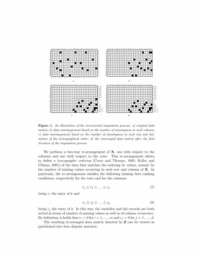
Figure 1. An illustration of the incremental imputation process: a) original datamatrix; b) data rearrangement based on the number of missingness in each column;c) data rearrangement based on the number of missingness in each row and def-inition of the lexicographical order; d) the rearranged data matrix after the firstiteration of the imputation process.

We perform a two-way re-arrangement of X, one with respect to thecolumns and one with respect to the rows. This re-arrangement allowsto define a lexicographic ordering (Cover and Thomas, 1991; Keller andUllman, 2001) of the data that matches the ordering by values, namely bythe number of missing values occurring in each row and column of X. Inparticular, the re-arrangement satisfies the following missing data rankingconditions, respectively for the rows and for the columns:

r1 ≤ r2 ≤ . . . ≤ rn (7)

being ri the entry of r and

c1 ≤ c2 ≤ . . . ≤ cp (8)

being cj the entry of c. In this way, the variables and the records are bothsorted in terms of number of missing values as well as of column occurrence.By definition, it holds that ri = 0 for i = 1, . . . ,m and cj = 0 for j = 1, . . . , d.

The resulting re-arranged data matrix denoted by Z can be viewed aspartitioned into four disjoint matrices:

Zn,p =

Am,d Cm,p−d

Bn−m,d Dn−m,p−d

where only the matrix D contains missing values while the other three blocksare completely observed in both rows and columns. By definition, withinthe uncomplete block D missing values are placed at different degrees ofmissing-ness from the right to left and from the upper part to the bottompart. In particular, if there exists only one variable presenting only one miss-ing data, then this variable results in the p-th column and the first imputedvalue will be found for the m + 1-th record. If there are two variables withonly one missing data then they are in the last two columns, and the first im-puted values will be found in the m+1-th record. A graphical representationof the above data pre-processing yielding to the matrix Z is given in figure 1.

3.2 The incremental imputation method

Once that the different types of missing-ness have been ranked and coded,the missing data imputation is iteratively made using tree based models.

The general idea is to use the complete part of Z to impute - via decisiontrees - the uncomplete one D, and on the basis of the lexicographic orderingthe imputed values enter in the complete part for the imputation of theremaining missing values.

In practice, the matrix Z can be viewed as structured into two sub-matrices Z = [Zobs|Zmis], where Zobs is the n × d complete part and Zmis

is the n× (p− d) uncomplete part. The latter is formed by the q = (p− d)variables presenting missing values, namely Zmis = [Zd+1, . . . ,Zp].

With respect to the records presenting only one missing data, a simpletree is used. Applying the tree-based procedure, each variable presentingmissing values is considered as response variable at turn, whereas the re-maining variables presenting either no missing values or imputed values areused as predictors. Whereas the first d variables in Zobs always enter aspredictors, the last q variables might enter either as a response or as a pre-dictor in the tree procedure. The decision tree is obtained applying cross-validation estimates of the error rate and considering the current completesample of objects. The results of the tree are used to impute the missingdata in D. In fact, terminal nodes of the tree represent candidate imputedvalues. Actual imputed values are get by dropping down the tree the casesof B corresponding to the missing values in D (for the variable under im-putation), till a terminal node is reached. The conjunction of the filled-incells of D with the corresponding observed rows in B generates new recordswhich are appended to A, that gains the rows whose missing values have

been just imputed and a “new” column corresponding to the variable underimputation.

For records presenting multiple missing values, trees are used iteratively.In this case, according to the previously defined lexicographic ordering, thetree is first used to fill in the missing values of the variables presenting thesmallest number of incomplete records. The procedure is then repeated forthe remaining variables under imputation. In this way, we form as manytrees as the number of variables with missing values in the given missing-ness. In the end, the imputation of joint missing-ness derives from subse-quent trees. A graphical description of the imputation of the first missingvalue is given in figure 2.

Figure 2. An illustration of the incremental imputation process: after the first it-

eration the row 10 becomes completely observed and the imputation process proceedthrough imputation of row 6.

A formal description of the proposed imputation process at any generic v-th iteration can be given as follows. Let yi∗,j∗ be the cell presenting a missinginput in the i∗-th row and the j ∗-th column of the matrix Z. The imputationderives from the tree grown from the sample Lv = {x′i, yi; i = 1, . . . , s} whereyi = zij∗ and x′i = (zi,1, . . . , zi,j , . . . , zi,p)′ such that rij = 0 for any couple(i, j). The imputation of the current missing data zi∗j∗ is obtained from thedecision rule d(x) = y.

Obviously due to the lexicographical order the imputation is made sep-arately for each set of rows presenting missing data in the same cells.

As a result, this imputation process is incremental, because as it goes onmore and more information is added to the data matrix, both respect therows and the columns. In other words, the matrices A, B and C are updatedin each iteration, and the additional information is used for imputing theremaining missing inputs. Equivalently, the matrix D containing missingvalues shrinks after each set of records with missing inputs has been filled-in. Furthermore, the imputation is also conditional because, in the jointimputation of multiple inputs, the subsequent imputations are conditionedon previously filled-in inputs.

3.3 The Incremental Imputation Algorithm (IIA)

From the computational point of view, some issues need to be considered inorder to implement the proposed imputation procedure.

Actually, the data re-arrangement of the matrix X yielding to Z is per-formed only at the beginning of the procedure, resulting in a data pre-processing step. In sub-sequent iterations, instead of sorting rows andcolumns of Z, the ri and the cj , in the conditions (??) and (??) respectively,are updated and used as pointers to identify the data under imputation. Itresults that the procedure stops when all the ri and the cj become zero.

It is worth mentioning a specific property derived from the lexicographicordering to rank missing data in each row of the matrix Z. At any v-thiteration, the procedure takes account of the row with the lowest numberof missing data. It can be shown that if a missing data is imputed withinthe i∗-th record then it follows that, in the subsequent iteration v + 1, anyfurther missing data within the same record will be necessarily imputed.

In the following, we outline the Incremental Imputation Algorithm (IIA)implementing the proposed methodology.

0. : Pre-Processing: Missing Data Ranking.

Let X be the data matrix.

Define the indicator matrix R with ij-the entry 1 if xij = 0 and zerootherwise.

Define the column vector r = R1 being the ri entry the number ofmissing values in the i-th record.

Define the row vector c = 1R being the cj entry the number of missingvalues in the j-th variable.

Apply the missing data ranking conditions (??) and (??) to the ma-trix X for both rows and columns in order to define the matrix Z =[Zobs|Zmis] or, equivalently, Z = [Z1 . . . ,Zd|Zd+1, . . . ,Zp]

1. : Initialize.

Fix v = 1, s = m and t = d.

2. : Row-block selection of missing records.

For i = s + 1, . . . , n, find min(ri) = l.

Define the row-block string vector k = [1, . . . , K] indicating the rowsfor that rk = l with K ≡ #[ri = l], namely the total number of rowswith l missing values.

3. : Column selection of response variable.

For j = t + 1, . . . , p, find j∗ ≡ argminj(cj) such that Zj has missingvalues within any of the K rows-block.

Identify the missing data cell (i∗, j∗) choosing the row i∗ correspondingto the column j∗ with the lowest number of missing data.

Define Y (v) = Zj∗ as the current response variable which i∗-th rowneeds to be imputed.

4. : Incremental imputation.

Define the decision tree using the sample Lv = {x′i, yi; i = 1, . . . , s}where yi = zij∗ and x′i = (zi,1, . . . , zi,j , . . . , zi,p)′ such that rij = 0 forany couple (i, j).

Impute the current missing data zi∗j∗ from the decision tree d(x) = y.

5. : Updating missing data ranking.

Fix v = v + 1 and s = s + 1.

Update R, r and c.

If cj = 0 for j > t then t = t− 1. Otherwise, continue.

6. : Check.

If s = n then stop, Otherwise, go to 2.

4 A simulation study

4.1 The simulation settings

We show the results of a simulation study considering several simulationsettings. In each setting, covariates are uniformly distributed in [0, 10] andvalues are missing with conditional probability:

ψ = {1 + exp[a + Xb]}−1

where X is the covariates matrix, a is a constant and b is a vector of coef-ficients (in either case some can be zero). When generating missing valueswith the function ψ, corresponding to the MAR process, we impose that

the existence of missing values depends only on some covariates. In particu-lar, we distinguish the case of missing values generation in nominal (binary)covariates (i.e. the nominal response case) from the case of missing valuesgeneration in numerical covariates (i.e. the numerical response case). Thedifferent simulation setting are summarized in table 1.In each simulation setting, we distinguish between the case of linear andnonlinear data. In practice, we generated 8 different data structures for thenumerical as well as the nominal response case. Among these, the first four(namely sim1, sim2, sim3 and sim4) presented missing data in two variables,whereas in the other cases missing data occur in three covariates. The vari-ables under imputation are generated according to a theoretical distribution(the normal distribution for the numerical case and the binomial distribu-tion in the binary case). In some cases (sim1, sim2, sim5 and sim6), theparameters characterizing the distribution of the missing values depend onsome covariates in a nonlinear way, whereas in the other cases the parame-ters characterizing the distribution of the variable with missing values canbe expressed as a linear combination of some of the covariates.Each experiment was performed with the goal of estimating the parameterscharacterizing the distribution of the variable under imputation. In par-ticular, for the numerical response case we estimate the mean µ and thestandard deviation σ whereas, for the binary response case, we focus on theestimation of the expected value π.Table 2 to 5 report the results of the estimated parameters from 100 in-dependent samples randomly drawn from the original distribution function.We tested the hypothesis that the proposed methodology works well for non-linear data. In this respect, the data were generated varying the number ofobservations (1000 or 5000) and their structure (linear or nonlinear).For comparison purposes, we estimate the quantities of interest for the Un-conditional Mean Imputation (UMI), the Parametric Imputation (PI), theNon Parametric Imputation (NPI) and the Incremental Non ParametricImputation (INPI) based on the algorithm described in section 3.3. PI isbased on linear least squares with constant variance while NPI is based ontree based models2. For each simulation setting we searched for the impu-tation method providing the best results.

2The terminal nodes are defined by means of the CART pruning method (Breiman etal, 1984) in the cross validation version.

Numerical responsen p missing variables

sim1.n 1000 10 Y1 ∼ N(X1 −X22 , exp(0.3X1 + 0.1X2))

sim2.n 5000 10 Y2 ∼ N(X3 −X24 , exp(−1 + 0.5(0.3X3 + 0.1X4)))

sim3.n 1000 10 Y1 ∼ N(X1 −X22 , 0.3X1 + 0.1X2)

sim4.n 5000 10 Y2 ∼ N(X3 −X24 ,−1 + 0.5(0.3X3 + 0.1X4))

sim5.n 1000 10 Y1 ∼ N(X1 −X22 , exp(0.3X1 + 0.1X2))

sim6.n 5000 10 Y2 ∼ N(X3 −X24 , exp(−1 + 0.5(0.3X3 + 0.1X4)))

Y3 ∼ N(X5 −X26 , exp(−1 + 0.5(0.2X5 + 0.3X6)))

sim7.n 1000 10 Y1 ∼ N(X1 −X22 , 0.3X1 + 0.1X2)

sim8.n 5000 10 Y2 ∼ N(X3 −X24 ,−1 + 0.5(0.3X3 + 0.1X4)

Y3 ∼ N(X5 −X26 ,−1 + 0.5(0.2X5 + 0.3X6)

Binary responsen p missing variables

sim1.c 1000 10 Y1 ∼ Bin(

exp(X1−X2)1+exp(X1−X2)

)

sim2.c 5000 10 Y2 ∼ Bin(

exp(Y1+X2−X3)1+exp(Y1+X2−X3)

)

sim3.c 1000 10 Y1 ∼ Bin(

X1−X20.75(1+X1−X2)

)

sim4.c 5000 10 Y2 ∼ Bin(∣∣∣ Y1+X2−X3

1.25(1+Y1+X2−X3)

∣∣∣)

sim5.c 1000 10 Y1 ∼ Bin(

exp(X1−X2)1+exp(X1−X2)

)

sim6.c 5000 10 Y2 ∼ Bin(

exp(Y1+X2−X3)1+exp(Y1+X2−X3)

)

Y3 ∼ Bin(

exp(Y1+X4−X5)1+exp(Y1+X4−X5)

)

sim7.c 1000 10 Y1 ∼ Bin(

X1−X20.75(1+X1−X2)

)

sim8.n 5000 10 Y2 ∼ Bin(∣∣∣ Y1+X2−X3

1.25(1+Y1+X2−X3)

∣∣∣)

Y3 ∼ Bin(∣∣∣ Y1+X4−X5

1.25(1+Y1+X4−X5)

∣∣∣)

Table 1. Simulation settings

4.2 The results

Table 2 and Table 3 report the results of the compared methods for the 8data sets concerning the binary response case. In each table, the row namedwith ”TRUE” shows the values of the parameters under imputation in thecomplete data, that is before generating missing values from condition speci-fied in section 4. In each table we reported in bold the estimated parametersthat are closer to the true values (first row of the table).What is evident from tables 2 and 3 is that INPI works particularly wellfor nonlinear data, namely those resulting from sim1.c, sim2.c, sim5.c andsim6.c. In this cases, it is surprising to notice that INPI provides good esti-mates simultaneously for all the parameters under imputation. Instead, inthe other there is no imputation method clearly outperforming the others.For the experiments concerning the numerical response case, results are re-

ported in tables 4 and 5. Also in this case, INPI seems to perform betterboth for the mean and the standard deviation for nonlinear data (sim1.n,sim2.n, sim5.n and sim6.n), despite the number of covariates under imputa-tion (two for data in table 4 and three for data in table 5). In the remainingcases, even if PI was supposed to perform better, the results do not indicateexplicitly a single outperforming method.

sim1.c sim2.c sim3.c sim4.cπ̂1 π̂2 π̂1 π̂2 π̂1 π̂2 π̂1 π̂2

TRUE 0.520 0.562 0.506 0.529 0.546 0.550 0.549 0.558UMI 0.750 0.680 0.740 0.616 0.540 0.552 0.536 0.554PI 0.570 0.612 0.589 0.472 0.606 0.570 0.622 0.630NPI 0.490 0.493 0.470 0.458 0.605 0.562 0.574 0.615INPI 0.513 0.571 0.497 0.498 0.597 0.558 0.562 0.601

Table 2. Estimated probabilities for the binary response case in data setspresenting missing values in 2 covariates ( 100 independent samples randomly

drawn from the original distribution function).

sim5.c sim6.cπ̂1 π̂2 π̂3 π̂1 π̂2 π̂3

TRUE 0.533 0.539 0.557 0.507 0.452 0.547UMI 0.691 0.618 0.686 0.722 0.692 0.690PI 0.653 0.510 0.503 0.632 0.546 0.556NPI 0.501 0.525 0.587 0.481 0.536 0.554INPI 0.540 0.530 0.570 0.500 0.501 0.552

sim7.c sim8.cπ̂1 π̂2 π̂3 π̂1 π̂2 π̂3

TRUE 0.537 0.897 0.889 0.574 0.895 0.895UMI 0.530 0.908 0.906 0.471 0.782 0.906PI 0.615 0.925 0.920 0.646 0.928 0.923NPI 0.611 0.923 0.932 0.498 0.927 0.918INPI 0.534 0.925 0.917 0.577 0.929 0.794

Table 3. Estimated probabilities for the binary response case in data setspresenting missing values in 3 covariates ( 100 independent samples randomly

drawn from the original distribution function).

sim1.n sim2.nµ̂1 µ̂2 σ̂1 σ̂2 µ̂1 µ̂2 σ̂1 σ̂2

TRUE -26.15 -28.39 33.61 29.92 -25.93 -28.26 33.68 29.81UMI -30.73 -39.76 36.80 31.12 -31.15 -40.43 37.36 30.80PI -28.97 -24.78 34.12 34.38 -27.51 -24.30 34.59 34.70NPI -27.63 -26.08 33.35 31.13 -28.23 -26.11 32.93 30.79INPI -26.64 -27.07 33.46 29.47 -25.99 -27.10 33.91 29.16

sim3.n sim4.nµ̂1 µ̂2 σ̂1 σ̂2 µ̂1 µ̂2 σ̂1 σ̂2

TRUE 0.29 0.03 4.46 4.61 -28.81 -28.16 30.15 30.00UMI 1.21 0.59 4.59 4.90 -31.79 -39.92 30.94 29.33PI 0.16 0.00 4.32 4.48 -28.14 -24.41 31.19 34.61NPI 1.54 1.03 4.23 4.43 -26.97 -26.92 30.47 31.08INPI 1.63 1.05 4.11 4.49 -26.81 -26.98 30.51 31.02

Table 4. Estimated means and standard deviations for the numerical responsecase in data sets presenting missing values in 2 covariates ( 100 independent

samples randomly drawn from the original distribution function).

sim5.nµ̂1 µ̂2 µ̂3 σ̂1 σ̂2 σ̂3

TRUE -28.99 -27.19 -28.19 32.94 29.01 30.12UMI -31.81 -26.87 -28.48 36.27 28.69 30.45PI -31.19 -26.93 -28.28 32.03 28.75 29.14NPI -28.37 -27.00 -28.01 33.34 28.84 30.29INPI -28.90 -27.16 -28.16 33.07 28.99 30.17

sim6.nµ̂1 µ̂2 µ̂3 σ̂1 σ̂2 σ̂3

TRUE -28.49 -28.72 -28.95 33.52 30.49 30.17UMI -32.07 -29.01 -29.06 37.55 30.96 30.26PI -26.00 -28.49 -29.00 34.20 30.22 30.03NPI -26.05 -28.54 -28.75 33.85 30.36 30.34INPI -27.51 -28.72 -28.97 33.54 30.46 30.15

sim7.nµ̂1 µ̂2 µ̂3 σ̂1 σ̂2 σ̂3

TRUE -28.65 -29.71 -29.44 29.77 29.99 31.09UMI -31.64 -29.95 -29.49 30.97 30.66 30.95PI -28.64 -30.01 -29.34 30.52 29.73 30.98NPI -26.36 -29.81 -29.45 30.35 30.08 31.05INPI -26.85 -29.87 -29.24 29.67 30.16 31.28

sim8.nµ̂1 µ̂2 µ̂3 σ̂1 σ̂2 σ̂3

TRUE -28.65 -29.71 -29.44 29.77 29.99 31.09UMI -31.64 -28.95 -29.49 30.97 30.66 30.95PI -28.64 -30.02 -24.34 30.52 29.73 30.98NPI -26.36 -29.82 -29.45 30.34 30.08 31.27INPI -27.91 -29.78 -29.35 29.61 30.15 31.05

Table 5. Estimated means and standard deviations for the numerical responsecase in data sets presenting missing values in 3 covariates ( 100 independent

samples randomly drawn from the original distribution function).

5 Evidence from real data

In addition to the simulation study, we have tested the proposed incre-mental imputation method on two real data sets from the UCI Repositoryof Machine Learning databases (www.ics.uci.edu/∼mlearn/MLRepository),namely the Mushroom dataset (8124 instances, 22 nominally valued at-tributes), and the Boston Housing dataset (506 instances, 13 real valuedand 1 binary attributes). For each data set, we have generated missing val-ues in 4 covariates, according to the MAR condition.Table 6 and 7 summarize the results of the estimated parameters for the co-

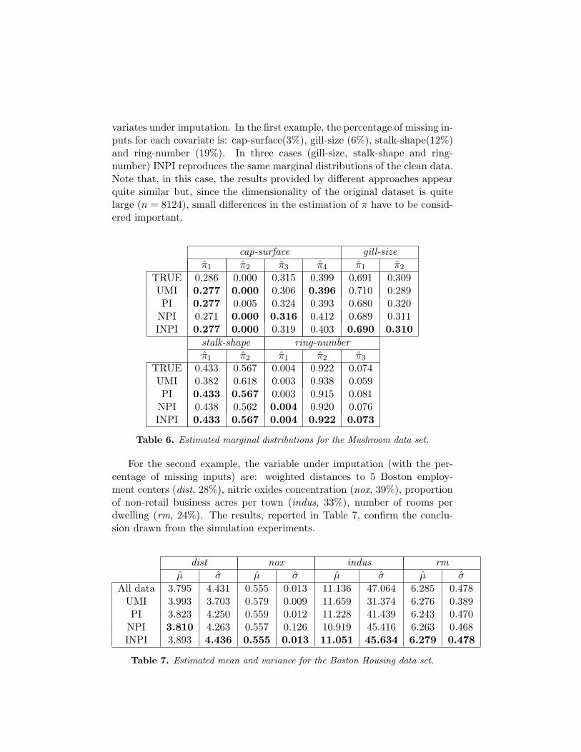
variates under imputation. In the first example, the percentage of missing in-puts for each covariate is: cap-surface(3%), gill-size (6%), stalk-shape(12%)and ring-number (19%). In three cases (gill-size, stalk-shape and ring-number) INPI reproduces the same marginal distributions of the clean data.Note that, in this case, the results provided by different approaches appearquite similar but, since the dimensionality of the original dataset is quitelarge (n = 8124), small differences in the estimation of π have to be consid-ered important.

cap-surface gill-sizeπ̂1 π̂2 π̂3 π̂4 π̂1 π̂2

TRUE 0.286 0.000 0.315 0.399 0.691 0.309UMI 0.277 0.000 0.306 0.396 0.710 0.289PI 0.277 0.005 0.324 0.393 0.680 0.320

NPI 0.271 0.000 0.316 0.412 0.689 0.311INPI 0.277 0.000 0.319 0.403 0.690 0.310

stalk-shape ring-numberπ̂1 π̂2 π̂1 π̂2 π̂3

TRUE 0.433 0.567 0.004 0.922 0.074UMI 0.382 0.618 0.003 0.938 0.059PI 0.433 0.567 0.003 0.915 0.081

NPI 0.438 0.562 0.004 0.920 0.076INPI 0.433 0.567 0.004 0.922 0.073

Table 6. Estimated marginal distributions for the Mushroom data set.

For the second example, the variable under imputation (with the per-centage of missing inputs) are: weighted distances to 5 Boston employ-ment centers (dist, 28%), nitric oxides concentration (nox, 39%), proportionof non-retail business acres per town (indus, 33%), number of rooms perdwelling (rm, 24%). The results, reported in Table 7, confirm the conclu-sion drawn from the simulation experiments.

dist nox indus rmµ̂ σ̂ µ̂ σ̂ µ̂ σ̂ µ̂ σ̂

All data 3.795 4.431 0.555 0.013 11.136 47.064 6.285 0.478UMI 3.993 3.703 0.579 0.009 11.659 31.374 6.276 0.389PI 3.823 4.250 0.559 0.012 11.228 41.439 6.243 0.470

NPI 3.810 4.263 0.557 0.126 10.919 45.416 6.263 0.468INPI 3.893 4.436 0.555 0.013 11.051 45.634 6.279 0.478

Table 7. Estimated mean and variance for the Boston Housing data set.

6 Conclusions

Tree-based methods have been increasing their popularity in various disci-plines due to several advantages: their non parametric nature, since they donot assume any underlying family of probability distributions; their flexibil-ity, because they handle simultaneously categorical and numerical predictorsand interactions among them; their simplicity, from a conceptual viewpoint,that is very useful for the definition of handy decision rules. From the ge-ometrical point of view, trees consider conditional interactions among vari-ables to define a partition of the feature space into a set of rectangles wheresimple models (like a constant) are fitted.

These advantages of trees have been exploited in the definition of theIncremental Non Parametric Imputation (INPI) for handling missing dataas described in the so called Incremental Imputation Algorithm (IIA). Thebasic assumption is that monotone missing data pattern are derived fromthe Missing At Random (MAR) mechanism. The proposed methodologyconsiders a lexicographic ordering of the missing data in order to performiteratively tree-based data imputation, yielding to a nonparametric condi-tional mean estimation. The resulting missing data imputation is performedincrementally because, in each iteration, the imputed values are added tothe completely observed ones and concur to the imputation of the remain-ing missing data. The results concerning the application of the proposedmethodology on both artificial and real data set, confirm its effectiveness,in most cases when data are nonlinear and heteroscedastic.

In our opinion, this approach might be part of the statistical learn-ing paradigm, aimed to extract important patterns and trends from vastamounts of data. In particular, we think that missing data represents a lossof information that can not be used for statistical purposes. Our method-ology can be understood as tool to do statistical learning by informationretrieval, namely to recapture missing data in order to improve the knowl-edge discovery process.

References

Breiman, L., Friedman, J.H., Olshen, R.A., and Stone, C.J. (1984). Classi-fication and Regression Trees. Monterey (CA): Wadsworth & Brooks.

Cappelli, C., Mola, F., and Siciliano, R. (2002). A Statistical Approach toGrowing a Reliable Honest Tree, Computational Statistics and DataAnalysis, 38, 285-299, Elsevier Science.

Cover, T.M., Thomas, J.A., (1991). Elements of Information Theory. NewYork: John Wiley and Sons.

Hastie, T., Tibshirani, R., Friedman, J. (2001). The Elements of StatisticalLearning. Springer, NY.

Ibrahim, J.G., Lipsitz, S.R., Chen, M.H. (1999). Missing Covariates inGeneralized Linear Models when the missing data mechanism is non-ignorable, Journal of the Royal Statistical Society, Series B, 61(1),173-190.

Keller, A.M., Ullman, J.D., (2001). A Version Numbering Scheme with aUseful Lexicographical Order, Technical Report, Stanford University.

Klaschka, J., Siciliano, R., and Antoch, J. (1998): Computational En-hancements in Tree-Growing Methods, Advances in Data Science andClassification: Proceedings of the 6th Conference of the InternationalFederation of Classification Society (Roma, July 21-24, 1998), (Rizzi,A., Vichi, M., Bock, H.H., eds.) Springer-Verlag, Berlin Heidelberg(D), 295-302.

Little, J.R.A. (1992). Regression with Missing X’s: A Review, Journal ofthe American Statistical Association, 87(420), 1227-1237.

Little, J.R.A, Rubin, D.B. (1987). Statistical Analysis with Missing Data,John Wiley and Sons, New York.

Mola, F., Siciliano, R. (1997): A Fast Splitting Procedure for ClassificationTrees Statistics and Computing 7, 208–216.

Mola, F., Siciliano, R. (2002). Factorial Multiple Splits in Recursive Par-titioning for Data Mining, Proceedings of International Conference onMultiple Classifier Systems (Roli, F., Kittler, J., eds) (Cagliari, June24-26, 2002), Lecture Notes in Computer Science, 118-126, Springer,Berlin.

Sarle, W.S. (1998), Prediction with Missing Inputs, Technical Report, SASInstitute.

Schafer, J. L., (1997). Analysis of Incomplete Multivariate Data, Chapman& Hall.

Siciliano, R., Mola, F. 2000): Multivariate Data Analysis through Clas-sification and Regression Trees. Computational Statistics and DataAnalysis, (32), Elsevier Science, 285–301.

Vach, W. (1994). Logistic Regression with Missing Values and Covariates,Lecture Notes in Statistics, vol. 86, Springer Verlag, Berlin.