Reordering rows for better compression: Beyond the lexicographic order

Reordering Rows for Better Compression: Beyond the LexicographicOrder

DANIEL LEMIRE, TELUQ

OWEN KASER, University of New Brunswick

EDUARDO GUTARRA, University of New Brunswick

Sorting database tables before compressing them improves the compression rate. Can we do better than the

lexicographical order? For minimizing the number of runs in a run-length encoding compression scheme,

the best approaches to row-ordering are derived from traveling salesman heuristics, although there is a

significant trade-off between running time and compression. A new heuristic, Multiple Lists, which is a

variant on Nearest Neighbor that trades off compression for a major running-time speedup, is a good

option for very large tables. However, for some compression schemes, it is more important to generate long

runs rather than few runs. For this case, another novel heuristic, Vortex, is promising. We find that we

can improve run-length encoding up to a factor of 3 whereas we can improve prefix coding by up to 80%:

these gains are on top of the gains due to lexicographically sorting the table. We prove that the new row

reordering is optimal (within 10%) at minimizing the runs of identical values within columns, in a few cases.

Categories and Subject Descriptors: E.4 [Coding and Information Theory]: Data compaction and com-

pression; H.4.0 [Information Systems Applications]: General

General Terms: Algorithms, Experimentation, Theory

Additional Key Words and Phrases: Compression, Data Warehousing, Gray codes, Hamming Distance,

Traveling Salesman Problem

1. INTRODUCTION

Database compression reduces storage while improving the performance of some queries. Itis commonly recommended to sort tables to improve the compressibility of the tables [Poessand Potapov 2003] or of the indexes [Lemire et al. 2010]. While it is not always possible oruseful to sort and compress tables, sorting is a critical component of some column-orientedarchitectures [Abadi et al. 2008; Holloway and DeWitt 2008]

At the simplest level, we model compressibility by counting runs of identical values withincolumns. Thus, we want to reorder rows to minimize the total number of runs, in all columns(§ 3). The lexicographical order is the most common row-reordering heuristic for this prob-lem.

Can we beat the lexicographic order? Engineers might be willing to spend extra timereordering rows—even for modest gains (10% or 20%)—if the computational cost is accept-able. Indeed, popular compression utilities such as bzip2 are often several times slower thanfaster alternatives (e.g., gzip) for similar gains.

Moreover, minimizing the number of runs is of theoretical interest. Indeed, it reduces tothe Traveling Salesman Problem (TSP) under the Hamming distance—an NP-hard prob-lem [Trevisan 1997; Ernvall et al. 1985] (§ 3.1). Yet there have been few attempts to designand study TSP heuristics with the Hamming distance and even fewer on large data sets.For the generic TSP, there are several well known heuristics (§ 3.2), as well as strategies toscale them up (§ 3.3). Inspired by these heuristics, we introduce the novel Multiple Listsheuristic (§ 3.3.1) which is designed with the Hamming distance and scalability in mind.

While counting runs is convenient, it is an incomplete model. Indeed, several compression

This work is supported by Natural Sciences and Engineering Research Council of Canada grants 261437and 155967 and a Quebec/NB Cooperation grant.Author’s addresses: D. Lemire, LICEF Research Center, TELUQ; O. Kaser and E. Gutarra, Dept. of CSAS,University of New Brunswick, Saint John.

arX

iv:1

207.

2189

v3 [

cs.D

B]

3 F

eb 2

014

:2 D. Lemire et al.

algorithms for databases may be more effective when there are many “long runs” (§ 4).Thus, instead of minimizing the number of runs of column values, we may seek to maxi-mize the number of long runs. We can then test the result with popular compression algo-rithms (§ 6.1). For this new problem, we propose two heuristics: Frequent-Component(§ 4.2), and Vortex (§ 4.3). Vortex is novel.

All our contributed heuristics have O(n log n) complexity when the number of columns isa constant. However, Multiple Lists uses a linear number of random accesses, making itprohibitive for very large tables: in such cases, we use table partitioning (§ 3.3.2).

We can assess these TSP heuristics experimentally under the Hamming distance (§ 5).Using synthetic data sets (uniform and Zipfian), we find that Vortex is a competitiveheuristic on Zipfian data. It is one of the best heuristics for generating long runs. Meanwhile,Multiple Lists offers a good compromise between speed and run minimization: it can evensurpass much more expensive alternatives. Unfortunately, it is poor at generating long runs.

Based on these good results, we apply Vortex and Multiple Lists to realistic tables,using various table-encoding techniques. We show that on several data sets both MultipleLists and Vortex can improve compression when compared to the lexicographical order—especially if the column histograms have high statistical dispersion (§ 6).

2. RELATED WORK

Many forms of compression in databases are susceptible to row reordering. For example,to increase the compression factor, Oracle engineers [Poess and Potapov 2003] recommendsorting the data before loading it. Moreover, they recommend taking into account the cardi-nality of the columns—that is, the number of distinct column values. Indeed, they indicatethat sorting on low-cardinality columns is more likely to increase the compression factor.Poess and Potapov do not quantify the effect of row reordering. However, they report thatcompression gains on synthetic data are small (a factor of 1.4 on TPC-H) but can be muchlarger on real data (a factor of 3.1). The effect on performance varies from slightly longerrunning times to a speedup of 38% on some queries. Loading times are doubled.

Column-oriented databases and indexes are particularly suitable for compression.Column-oriented databases such as C-Store use the conventional (lexicographical) sort toimprove compression [Stonebraker et al. 2005; Abadi et al. 2006]. Specifically, a given tableis decomposed into several overlapping projections (e.g., on columns 1,2,3 then on column2,3,4) which are sorted and compressed. By choosing projections matching the query work-load, it is possible to surpass a conventional DBMS by orders of magnitude. To validatetheir model, Stonebraker et al. used TPC-H with a scale factor of 10: this generated 60 mil-lion rows in the main table. They kept only attributes of type INTEGER and CHAR(1).On this data, they report a total space usage of 2 GB compared to 2.7 GB for an alternativecolumn store. They have a 30% storage advantage, and better performance, partly becausethey sort their projections before compressing them.

Lemire and Kaser [2011] prove that sorting the projections on the low-cardinality columnfirst often maximizes compression.They stress that picking the right column order is impor-tant as the compressibility could vary substantially (e.g., by a factor of 2 or 3). They considervarious alternatives to the lexicographical order such as modular and reflected Gray-codeorders or Hilbert orders, and find them ineffective. In contrast, we propose new heuristics(Vortex and Multiple Lists) that can surpass the lexicographical order. Indeed, whenusing a compression technique such as Prefix coding (see § 6.1.1), Lemire and Kaser obtaincompression gains of more than 20% due to sorting: using the same compression technique,on the same data set, we report further gains of 21%. Pourabbas et al. [2012] extend thestrategy by showing that columns with the same cardinality should be ordered from highskewness to low skewness.

The compression of bitmap indexes also greatly benefits from table sorting. In some exper-iments, the sizes of the bitmap indexes are reduced by nearly an order of magnitude [Lemire

Reordering Rows for Better Compression: Beyond the Lexicographic Order :3

et al. 2010]. Of course, everything else being equal, smaller indexes tend to be faster. Mean-while, alternatives to the lexicographical order such as Frequent-Component, reflectedGray-code or Hilbert orders are unhelpful on bitmap indexes [Lemire et al. 2010]. (Wereview an improved version of Frequent-Component in § 4.2.)

Still in the context of bitmap indexes, Malik and Kender [2007] get good compressionresults using a variation on the Nearest Neighbor TSP heuristic. Unfortunately, its quadratictime complexity makes the processing of large data sets difficult. To improve scalability,Malik and Kender [2007] also propose a faster heuristic called aHDO which we review in§ 3.2. In comparison, our novel Multiple Lists heuristic is also an attempt to get a morescalable Nearest Neighbor heuristic. Malik and Kender used small data sets having between204 rows and 34 389 rows. All their compressed bitmap indexes were under 10 MB. On theirlargest data set, the compression gain from aHDO was 14% when compared to the originalorder. Sorting improved compression by 7%, whereas their Nearest Neighbor TSP heuristichad the best gain at 17%. Pinar et al. [2005] also present good compression results on bitmapindexes after reordering: on their largest data set (11 MB), they report using a Gray-codeapproach to get a compression ratio of 1.64 compared to the original order. Unfortunately,they do not compare with the lexicographical order.

Sometimes reordering all of the data before compression is not an option. For example,Fusco et al. [2010; 2012] describe a system where bitmap indexes must be compressed on-the-fly to index network traffic. They report that their system can accommodate the insertionof more than a million records per second. To improve compressibility without sacrificingperformance, they cluster the rows using locality sensitive hashing [Gionis et al. 1999]. Theyreport a compression factor of 2.7 due to this reordering (from 845 MB to 314 MB).

3. MINIMIZING THE NUMBER OF RUNS

One of the primary benefits of column stores is the compression due to run-length encoding(RLE) [Abadi et al. 2008; Bruno 2009; Holloway and DeWitt 2008]. Moreover, the mostpopular bitmap-index compression techniques are variations on RLE [Wu et al. 2006].

RLE is a compression strategy where runs of identical values are coded using the repeatedvalue and the length of the run. For example, the sequence aaaaabcc becomes 5 × a, 1 ×b, 2 × c. Counters may be stored using a variable number of bits, e.g., using variable-bytecoding [Scholer et al. 2002; Bhattacharjee et al. 2009], Elias delta coding [Scholer et al.2002] or Golomb coding [Golomb 1966]. Or we may store counters using a fixed number ofbits for faster decoding.

RLE not only reduces the storage requirement: it also reduces the processing time. Forexample, we can compute the component-wise sum—or indeed any O(1) operation—oftwo RLE-compressed array in time proportional to the total number of runs. In fact, wesometimes sacrifice compression in favor of speed:

— to help random access, we can add the row identifier to the run length and repeatedvalue [Abadi et al. 2006] so that 5×a, 1×b, 2× c becomes 5×a at 1, 1×b at 6, 2× c at 7;

— to simplify computations, we can forbid runs from different columns to partially over-lap [Bruno 2009]: unless two runs are disjoint as sets of row identifiers, then one must bea subset of the other;

— to avoid the overhead of decoding too many counters, we may store single values or shortruns verbatim—without any attempt at compression [Antoshenkov 1995; Wu et al. 2006].

Thus, instead of trying to model each form of RLE compression accurately, we only countthe total number of runs (henceforth RunCount).

Unfortunately, minimizing RunCount by row reordering is NP-hard [Lemire and Kaser2011; Olken and Rotem 1986]. Therefore, we resort to heuristics. We examine many possiblealternatives (see Table I).

:4 D. Lemire et al.

Table I: Summary of heuristics considered and overall results. Not all methods were testedon realistic data; those not tested were either too inefficient for large data, or were clearlyunpromising after testing on Zipfian data.

Name Reference DescribedExperiments

Synthetic Realistic

1-reinsertion [Pinar and Heath 1999] § 3.2 § 5 —

aHDO [Malik and Kender 2007] § 3.2 § 5 —

BruteForcePeephole novel § 3.2 § 5 —

Farthest Insertion,Nearest Insertion,Random Insertion

[Rosenkrantz et al. 1977] § 3.2 § 5 —

Frequent-Component [Lemire et al. 2010] § 4.2 § 5 —

Lexicographic Sort — § 3 § 5 § 6.4

Multiple Fragment [Bentley 1992] § 3.2 § 5 —

Multiple Lists novel § 3.3.1 § 5 § 6.4

Nearest Neighbor [Bellmore and Nemhauser 1968] § 3.2 § 5 —

Savings [Clarke and Wright 1964] § 3.2 § 5 —

Vortex novel § 4.3 § 5 § 6.4

An effective heuristic for the RunCount minimization problem is to sort the rows inlexicographic order. In the lexicographic order, the first component where two tuples differ(aj 6= bj but ai = bi for i < j) determines which tuple is smaller.

There are alternatives to the lexicographical order. A Gray code is an ordered list oftuples such that the Hamming distance between successive tuples is one.1 The Hammingdistance is the number of different components between two same-length tuples, e.g.,

d( (a, b, y), (a, d, x) ) = 2.

The Hamming distance is a metric: i.e., d(x, x) = 0, d(x, y) = d(y, x) and d(x, y) +d(y, z) ≥d(x, z). A Gray code over all possible tuples generates an order (henceforth a Gray-codeorder): x < y whenever x appears before y in the Gray code. For example, we can use themixed-radix reflected Gray-code order [Richards 1986; Knuth 2011] (henceforth ReflectedGC). Consider a two-column table with column cardinalities N1 and N2. We label thecolumn values from 1 to N1 and 1 to N2. Starting with the tuple (1, 1), we generate alltuples in Reflected GC order by the following algorithm:

— If the first component is odd then if the second component is less than N2, increment it,otherwise increment the first component.

— If the first component is even then if the second component is greater than 1, decrementit, otherwise increment the first component.

E.g., the following list is in Reflected GC order:

(1, 1), (1, 2), . . . , (1, N2), (2, N2), (2, N2 − 1), . . . , (2, 1), (3, 1), . . .

The generalization to more than two columns is straightforward. Unfortunately, the benefitsof Reflected GC compared to the lexicographic order are small [Malik and Kender 2007;Lemire and Kaser 2011; Lemire et al. 2010].

We can bound the optimality of lexicographic orders using only the number of rows andthe cardinality of each column. Indeed, for the problem of minimizing RunCount by rowreordering, lexicographic sorting is µ-optimal [Lemire and Kaser 2011] for a table with

1For a more restrictive definition, we can replace the Hamming distance by the Lee metric [Anantha et al.2007].


n distinct rows and column cardinalities Ni for i = 1, . . . , c with

µ =

∑cj=1 min(n,

∏jk=1Nk)

n+ c− 1.

To illustrate this formula, consider a table with 1 million distinct rows and four columns hav-ing cardinalities 10, 100, 1000, 10000. Then, we have µ ≈ 2 which means that lexicographicsorting is 2-optimal. To apply this formula in practice, the main difficulty might be to de-termine the number of distinct rows, but there are good approximation algorithms [Aouicheand Lemire 2007; Kane et al. 2010]. We can improve the bound µ slightly:

Lemma 3.1. For the RunCount minimization problem, sorting the table lexicographi-cally is ω-optimal for

ω =

∑ci=1 n1,i

n+ c− 1

where c is the number of columns, n is the number of distinct rows, and n1,j is the numberof distinct rows when considering only the first j columns (e.g., n = n1,c).

Proof. Irrespective of the order of the rows, there are at least n+c−1 runs. Yet, underthe lexicographic order, there are no more than n1,i runs in the ith column. The resultfollows.

The bound ω is tight. Indeed, consider a table with N1, N2, . . . , Nc distinct values incolumns 1, 2, . . . , c and such that it has n = N1N2 . . . Nc distinct rows. The lexicographicorder will generate N1+N1N2+ · · ·+N1N2 . . . Nc runs. In the notation of Lemma 3.1, thereare

∑ci=1 n1,i runs. However, we can also order the rows so that there are only n+c−1 runs

by using the Reflected GC order.We have that ω is bounded by the number of columns. That is, we have that 1 ≤ ω ≤ c.

Indeed, we have that n1,c = n and n1,i ≥ 1 so that∑c

i=1 n1,i ≥ n+ c− 1 and therefore

ω =∑c

i=1 n1,i

n+c−1 ≥ 1. We also have that n1,i ≤ n so that∑c

i=1 n1,i ≤ cn ≤ c(n + c − 1) and

hence ω =∑c

i=1 n1,i

n+c−1 ≤ c. In practice, the bound ω is often larger when c is larger (see § 6.2).

3.1. Run minimization and TSP

There is much literature about the TSP, including approximation algorithms and manyheuristics, but our run-minimization problem is not quite the TSP: it more resembles aminimum-weight Hamiltonian path problem because we do not complete the cycle [Choand Hong 2000]. In order to use known TSP heuristics, we need a reduction from ourproblem to TSP. In particular, we reduce the run-minimization problem to TSP over theHamming distance d. Given the rows r1, r2, . . . , rn, RunCount for c columns is given bythe sum of the Hamming distance between the successive rows,

c+

n−1∑i=1

d(ri, ri+1).

Our goal is to minimize∑n−1

i=1 d(ri, ri+1). Introduce an extra row r? with the property thatd(r?, ri) = c for any i. We can achieve the desired result under the Hamming distance byfilling in the row r? with values that do not appear in the other rows. We solve the TSPover this extended set (r1, . . . , rn, r?) by finding a reordering of the elements (r′1, . . . , r

′n, r?)

minimizing the sum of the Hamming distances between successive rows:

d(r′n, r?) + d(r?, r′1) +

n−1∑i=1

d(r′i, r′i+1) = 2c+

n−1∑i=1

d(r′i, r′i+1).

:6 D. Lemire et al.

Any reordering minimizing 2c+∑n−1

i=1 d(r′i, r′i+1) also minimizes

∑n−1i=1 d(r′i, r

′i+1). Thus, we

have reduced the minimization of RunCount by row reordering to TSP. Heuristics forTSP can now be employed for our problem—after finding a tour (r′1, . . . , r

′n, r?), we order

the table rows as r′1, r′2, . . . , r

′n.

Unlike the general TSP, we know of linear-time c-optimal heuristics when using the Ham-ming distance. An ordering is discriminating [Cai and Paige 1995] if duplicates are listedconsecutively. By constructing a hash table, we can generate a discriminating order in ex-pected linear time. It is sufficient for c-optimality.

Lemma 3.2. Any discriminating row ordering is c-optimal for the RunCount mini-mization problem.

Proof. If n is the number of distinct rows, then a discriminating row ordering has atmost nc runs. Yet any ordering generates at least n runs. This proves the result.

Moreover—by the triangle inequality—there is a discriminating row order minimizingthe number of runs. In fact, given any row ordering we can construct a discriminatingrow ordering with a lesser or equal cost

∑n−1i=1 d(ri, ri+1) because of the triangle inequality.

Formally, suppose that we have a non-discriminating order r1, r2, . . . , rn. We can find twoidentical tuples (rk = rj) separated by at least one different tuple (rk+1 6= rj). Suppose j <

n. If we move rj between rk and rk+1, the cost∑n−1

i=1 d(ri, ri+1) will change by d(rj−1, rj+1)−(d(rj−1, rj) + d(rj , rj+1)): a quantity at most zero by the triangle inequality. If j = n, thecost will change by −d(rj−1, rj), another non-positive quantity. We can repeat such movesuntil the new order is discriminating, which proves the result.

3.2. TSP heuristics

We want to solve TSP instances with the Hamming distance. For such metrics, oneof the earliest and still unbeaten TSP heuristics is the 1.5-optimal Christofides algo-rithm [Christofides 1976; Berman and Karpinski 2006; Gharan et al. 2011]. Unfortunately,it runs in O(n2.5(log n)1.5) time [Gabow and Tarjan 1991] and even a quadratic runningtime would be prohibitive for our application.2

Thus, we consider faster alternatives [Johnson and McGeoch 2004; Johnson and McGeoch1997].

— Some heuristics are based on space-filling curves [Platzman and Bartholdi 1989]. In-tuitively, we want to sort the tuples in the order in which they would appear on a curvevisiting every possible tuple. Ideally, the curve would be such that nearby points on thecurve are also nearby under the Hamming distance. In this sense, lexicographic orders—aswell as the Vortex order (see § 4.3)—belong to this class of heuristics even though they arenot generally considered space-filling curves. Most of these heuristics run in time O(n log n).

— There are various tour-construction heuristics [Johnson and McGeoch 2004]. Theseheuristics work by inserting, or appending, one tuple at a time in the solution. In this sense,they are greedy heuristics. They all begin with a randomly chosen starting tuple. Thesimplest is Nearest Neighbor [Bellmore and Nemhauser 1968]: we append an availabletuple, choosing one of those nearest to the last tuple added. It runs in time O(n2) (seealso Lemma 3.3). A variation is to also allow tuples to be inserted at the beginning of thelist or appended at the end [Bentley 1992]. Another similar heuristic is Savings [Clarkeand Wright 1964] which is reported to work well with the Euclidean distance [Johnson andMcGeoch 2004]. A subclass of the tour-construction heuristics are the insertion heuristics:

2Unless we explicitly include the number of columns c in the complexity analysis, we consider it to be aconstant.


the selected tuple is inserted at the best possible location in the existing tour. They differin how they pick the tuple to be inserted:— Nearest Insertion: we pick a tuple nearest to a tuple in the tour.— Farthest Insertion: we pick a tuple farthest from the tuples in the tour.— Random Insertion: we pick an available tuple at random.One might also pick a tuple whose cost of insertion is minimal, leading to an O(n2 log n)heuristic. Both this approach and Nearest Insertion are 2-optimal, but the named in-sertion heuristics are in O(n2) [Rosenkrantz et al. 1977]. There are many variations [Kahngand Reda 2004].

— Multiple Fragment (or Greedy) is a bottom-up heuristic: initially, each tupleconstitutes a fragment of a tour, and fragments of tours are repeatedly merged [Bentley1992]. The distance between fragments is computed by comparing the first and last tuplesof both fragments. Under the Hamming distance, there is a c + 1-pass implementationstrategy: first merge fragments with Hamming distance zero, then merge fragments withHamming distance one and so on. It runs in time O(n2c2).

— Finally, the last class of heuristics are those beginning with an existing tour. Wecontinue trying to improve the tour until it is no longer possible or another stopping criteriais met. There are many “tour-improvement techniques” [Helsgaun 2000; Applegate et al.2003]. Several heuristics break the tour and attempt to reconstruct a better one [Croes 1958;Lin and Kernighan 1973; Helsgaun 2000; Applegate et al. 2003].Malik and Kender [2007] propose the aHDO heuristic which permutes successive tuples toimprove the solution. Pinar et al. [2005] describe a similar scheme, where they considerpermuting tuples that are not immediately adjacent, provided that they are not too farapart. Pinar and Heath [1999] repeatedly remove and reinsert (henceforth 1-Reinsertion)a single tuple at a better location. A variation is the BruteForcePeephole heuristic:divide up the table into small non-overlapping partitions of rows, and find the optimalsolution that leaves the first and last row unchanged (that is, we solve a Traveling SalesmanPath Problem (TSPP) [Lam and Newman 2008]).

3.3. Scaling up the heuristics

External-memory sorting is applicable to very large tables. However, even one of the fastestTSP heuristics (Nearest Neighbor) may fail to scale. We consider several strategies toalleviate this scalability problem.

3.3.1. Sparse graph. Instead of trying to solve the problem over a dense graph, where everytuple can follow any other tuple in the tour, we may construct a sparse graph [Reinelt 1994;Johnson et al. 2004]. For example, the sparse graph might be constructed by limiting eachtuple to some of its near neighbors. A similar approach has also been used, for example,in the design of heuristics in weighted matching [Grigoriadis and Kalantari 1988] and fordocument identifier assignment [Ding et al. 2010]. In effect, we approximate the nearestneighbors.

We consider a similar strategy. Instead of storing a sparse graph structure, we storethe table in several different orders. We compare rows only against other rows appearingconsecutively in one of the lists. Intuitively, we consider rows appearing consecutively insorted lists to be approximate near neighbors [Indyk and Motwani 1998; Gionis et al. 1999;Indyk et al. 1997; Chakrabarti et al. 1999; Liu 2004; Kushilevitz et al. 1998]. We implementedan instance of this strategy (henceforth Multiple Lists).

Before we formally describe the Multiple Lists heuristic, consider the example givenin Fig. 1. Starting from an initial table (Fig. 1a), we sort the table lexicographically withthe first column as the primary key: this forms a list which we represent as solid edges inthe graph of Fig. 1c. Then, we re-sort the table, this time using the second column as theprimary key: this forms a second list which we represent as dotted edges in Fig. 1c. Finally,

:8 D. Lemire et al.

1 32 12 23 34 14 25 36 16 27 48 3

(a) Initial table

1 33 35 38 37 46 26 14 14 22 22 1

(b) Possible solution

1,3

2,1

3,3

2,2

4,14,25,3

6,1

6,28,3

7,4

(c) Multiply-linked list

Fig. 1: Row-reordering example with Multiple Lists

starting from one particular row (say 1,3), we can greedily pick a nearest neighbor (say 3,3)within the newly created sparse graph. We repeat this process iteratively (3,3 goes to 5,3and so on) until we have the solution given in Fig. 1b.

Hence, to apply Multiple Lists we pick several different ways to sort the table. For eachtable order, we store the result in a dynamic data structure so that rows can be selectedin order and removed quickly. (Duplicate rows can be stored once if we keep track of theirfrequencies.) One implementation strategy uses a multiply-linked list. Let K be the numberof different table orders. Add to each row room for 2K row pointers. First sort the rowin the first order. With pointers, link the successive rows, as in a doubly-linked list—using2 pointers per row. Resort the rows in the second order. Link successive rows, using another2 pointers per row. Continue until all K orders have been processed and every row has2K pointers. Removing a row in this data structure requires the modification of up to4K pointers.

For our experiments, we applied Multiple Lists with K = c as follows. First sort thetable lexicographically3 after ordering the columns by non-decreasing cardinalities (N1 ≤N2 ≤ · · · ≤ Nc). Then rotate the columns cyclically so that the first column becomes thesecond one, the second one becomes the third one, and the last column becomes the first:

3Sorting with reflected Gray code yielded no appreciable improvement on Zipfian data.


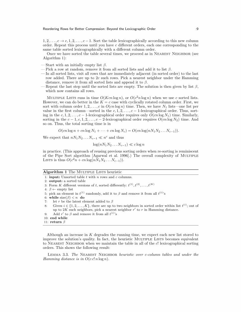
1, 2, . . . , c→ c, 1, 2, . . . , c− 1. Sort the table lexicographically according to this new columnorder. Repeat this process until you have c different orders, each one corresponding to thesame table sorted lexicographically with a different column order.

Once we have sorted the table several times, we proceed as in Nearest Neighbor (seeAlgorithm 1):

— Start with an initially empty list β.— Pick a row at random, remove it from all sorted lists and add it to list β.— In all sorted lists, visit all rows that are immediately adjacent (in sorted order) to the last

row added. There are up to 2c such rows. Pick a nearest neighbor under the Hammingdistance, remove it from all sorted lists and append it to β.

— Repeat the last step until the sorted lists are empty. The solution is then given by list β,which now contains all rows.

Multiple Lists runs in time O(Kcn log n), or O(c2n log n) when we use c sorted lists.However, we can do better in the K = c case with cyclically rotated column order. First, wesort with column order 1, 2, . . . , c in O(cn log n) time. Then, we have N1 lists—one list pervalue in the first column—sorted in the c, 1, 2, . . . , c − 1-lexicographical order. Thus, sort-ing in the c, 1, 2, . . . , c− 1-lexicographical order requires only O(cn logN1) time. Similarly,sorting in the c − 1, c, 1, 2, . . . , c − 2-lexicographical order requires O(cn logN2) time. Andso on. Thus, the total sorting time is in

O(cn log n+ cn logN1 + · · ·+ cn logNc) = O(cn log(nN1N2 . . . Nc−1)).

We expect that nN1N2 . . . Nc−1 � nc and thus

log(nN1N2 . . . Nc−1)� c log n

in practice. (This approach of reusing previous sorting orders when re-sorting is reminiscentof the Pipe Sort algorithm [Agarwal et al. 1996].) The overall complexity of MultipleLists is thus O(c2n+ cn log(nN1N2 . . . Nc−1)).

Algorithm 1 The Multiple Lists heuristic

1: input: Unsorted table t with n rows and c columns.2: output: a sorted table3: Form K different versions of t, sorted differently: t(1), t(2), . . . , t(K)

4: β ← empty list5: pick an element in t(1) randomly, add it to β and remove it from all t(i)’s6: while size(β) < n do7: let r be the latest element added to β8: Given i ∈ {1, 2, . . . ,K}, there are up to two neighbors in sorted order within list t(i); out of

up to 2K such neighbors, pick a nearest neighbor r′ to r in Hamming distance.9: Add r′ to β and remove it from all t(i)’s10: end while11: return β

Although an increase in K degrades the running time, we expect each new list stored toimprove the solution’s quality. In fact, the heuristic Multiple Lists becomes equivalentto Nearest Neighbor when we maintain the table in all of the c! lexicographical sortingorders. This shows the following result:

Lemma 3.3. The Nearest Neighbor heuristic over c-column tables and under theHamming distance is in O(c c!n log n).

:10 D. Lemire et al.

When there are many columns (c > 4), constructing and maintaining c! lists might beprohibitive. Through informal tests, we found that maintaining c different sort orders is agood compromise. For c ≤ 2, Multiple Lists with c sorted lists is already equivalent toNearest Neighbor.

Unfortunately, our implementation of Multiple Lists is not suited to an external-memory implementation without partitioning.

3.3.2. Partitioning. Several authors partition—or cluster—the tuples before applying a TSPheuristic. [Cesari 1996; Reinelt 1994; Karp 1977; Johnson et al. 2004; Schaller 1999] Usingdatabase terminology, they partition the table horizontally. We explore this approach. Thecontent of the horizontal partitions depends on the original order of the rows: the first rowsare in the first partition and so on. Hence, we are effectively considering a tour-improvementtechnique: starting from an existing row ordering, we partition it and try to reduce thenumber of runs within each partition. For example, we can partition a lexicographicallysorted table and process each partition in main memory using expensive heuristics such asNearest Neighbor or random-access-intensive heuristics such as Multiple Lists.

We can process each partition independently: the problem is embarrassingly parallel. Ofcourse, this ignores runs created at the boundary between partitions.

Sometimes, we know the final row of the previous partition. In such cases, we mightchoose the initial row in the current partition to have a small Hamming distance with thelast row in the previous partition. In any case, this boundary effect becomes small as thesizes of the partitions grow.

Another immediate practical benefit of the horizontal partitioning is that we have ananytime—or interruptible—algorithm [Dean and Boddy 1988]. Indeed, we progressivelyimprove the row ordering, but can also abort the process at any time without losing thegains achieved up to that point.

We could ensure that the number of runs is always reduced. Indeed, whenever the ap-plication of the heuristic on the partition makes matter worse, we can revert back to theoriginal tuple order. Similarly, we can try several heuristics on each partition and pick thebest. And probabilistic heuristics such as Nearest Neighbor can be repeated. Moreover,we can repartition the table: e.g., each new partition—except the first and the last—cantake half its tuples from each of the two adjacent old partitions [Johnson and McGeoch1997].

For simplicity, we can use partitions having a fixed number of rows (except maybe forthe last partition). As an alternative, we could first sort the data and then create partitionsbased on the value of one or several columns. Thus, for example, we could ensure that allrows within a partition have the same value in one or several columns.

4. MAXIMIZING THE NUMBER OF LONG RUNS

It is convenient to model database compression by the number of runs (RunCount). How-ever, this model is clearly incomplete. For example, there is some overhead correspondingto each run of values we need to code: short runs are difficult to compress.

4.1. Heuristics for long runs

We developed a number of row-reordering heuristics whose goal was to produce long runs.Two straightforward approaches did not give experimental results that justified their costs.

One is due to an idea of Malik and Kender [2007]. Consider the Nearest Neighbor TSPheuristic. Because we use the Hamming distance, there are often several nearest neighborsfor the last tuple added. Malik and Kender proposed a modification of Nearest Neighborwhere they determine the best nearest neighbor based on comparisons with the previoustuples—and not only with the latest one. We considered many variations on this idea, andnone of them proved consistently beneficial: e.g., when there are several nearest neighbors


1 32 12 23 34 14 25 36 16 27 48 3

(a) Initial table

(1,1,1) (4,2,3)(2,1,2) (3,2,1)(2,1,2) (3,2,2)(1,1,3) (4,2,3)(2,1,4) (3,2,1)(2,1,4) (3,2,2)(1,1,5) (4,2,3)(2,1,6) (3,2,1)(2,1,6) (3,2,2)(1,1,7) (1,2,4)(1,1,8) (4,2,3)

(b) (f(vi), i, vi)

(4,2,3) (1,1,1)(3,2,1) (2,1,2)(3,2,2) (2,1,2)(4,2,3) (1,1,3)(3,2,1) (2,1,4)(3,2,2) (2,1,4)(4,2,3) (1,1,5)(3,2,1) (2,1,6)(3,2,2) (2,1,6)(1,2,4) (1,1,7)(4,2,3) (1,1,8)

(c) (f(vi), i, vi) (sorted)

(1,2,4) (1,1,7)(3,2,1) (2,1,2)(3,2,1) (2,1,4)(3,2,1) (2,1,6)(3,2,2) (2,1,2)(3,2,2) (2,1,4)(3,2,2) (2,1,6)(4,2,3) (1,1,1)(4,2,3) (1,1,3)(4,2,3) (1,1,5)(4,2,3) (1,1,8)

(d) Sorted triples

7 42 14 16 12 24 26 21 33 35 38 3

(e) Solution

Fig. 2: Row-reordering example with Frequent-Component

to the latest tuple, we tried reducing the set to a single tuple by removing the tuples thatare not also nearest to the second last tuple, and then removing the tuples that are not alsonearest to the third last tuple, and so on.

A novel heuristic, Iterated Matching, was also developed but found to be too ex-pensive for the quality of results typically obtained. It is based on the observation thata weighted-matching algorithm can form pairs of rows that have many length-two runs.Pairs of rows can themselves be matched into collections of four rows with many length-four runs, etc. Unfortunately, known maximum-matching algorithms are expensive and theexperimental results obtained with this heuristic were not promising. Details can be foundelsewhere [Lemire et al. 2012].

4.2. The Frequent-Component order

Intuitively, we would like to sort rows so that frequent values are more likely to appearconsecutively. The Frequent-Component [Lemire et al. 2010] order follows this intuition.

As a preliminary step, we compute the frequency f(v) of each column value v within eachof the c columns. Given a tuple, we map each component to the triple (frequency, column in-dex, column value).4 Thus, from the c components, we derive c triples (see Figs. 2a and 2b):e.g., given the tuple (v1, v2, v3), we get the triples ((f(v1), 1, v1), (f(v2), 2, v2), (f(v3), 3, v3)).We then lexicographically sort the triples, so that the triple corresponding to a most-frequent column value appears first—that is, we sort in reverse lexicographical order (seeFig. 2c): e.g., assuming that f(v3) < f(v1) < f(v2), the triples appear in sorted order as((f(v2), 2, v2), (f(v1), 1, v1), (f(v3), 3, v3)). The new tuples are then compared against eachother lexicographically over the 3c values (see Fig. 2d). When sorting, we can precomputethe ordered lists of triples for speed. As a last step, we reconstruct the solution from thelist of triples (see Fig. 2e).

Consider a table where columns have uniform histograms: given n rows and a columnof cardinality Ni, each value appears n/Ni times. In such a case, Frequent-Componentbecomes equivalent to the lexicographic order with the columns organized in non-decreasingcardinality.

4.3. Vortex: a novel order

The Frequent-Component order has at least two inconveniences:

4This differs slightly from the original presentation of the order [Lemire et al. 2010] where the column valueappeared before the column index.


1 11 21 31 42 12 22 32 43 13 23 33 44 14 24 34 4

(a) Lexicographic

1 11 21 31 42 42 32 22 13 13 23 33 44 44 34 24 1

(b) Reflected GC

1 41 31 21 14 13 12 12 42 32 24 23 23 43 34 34 4

(c) Vortex

1 11 22 22 12 32 41 41 33 33 44 44 34 14 23 23 1

(d) z-order withGray codes

1 12 12 21 21 31 42 42 33 33 44 44 34 23 23 14 1

(e) Hilbert

Fig. 3: Two-column tables sorted in various orders

— Given c columns having N distinct values apiece, a table where all possible rows arepresent has N c distinct rows. In this instance, Frequent-Component is equivalent to thelexicographic order. Thus, its RunCount is N c+N c−1+· · ·+1. Yet a better solution wouldbe to sort the rows in a Gray-code order, generating only N c +c−1 runs. For mathematicalelegance, we would rather have Gray-code orders even though the Gray-code property maynot enhance compression in practice.

— The Frequent-Component order requires comparisons between the frequencies ofvalues that are in different columns. Hence, we must at least maintain one ordered list ofvalues from all columns. We would prefer a simpler alternative with less overhead.

Thus, to improve over Frequent-Component, we want an order that considers thefrequencies of column values and yet is a Gray-code order. Unlike Frequent-Component,we would prefer that it compare frequencies only between values from the same column.

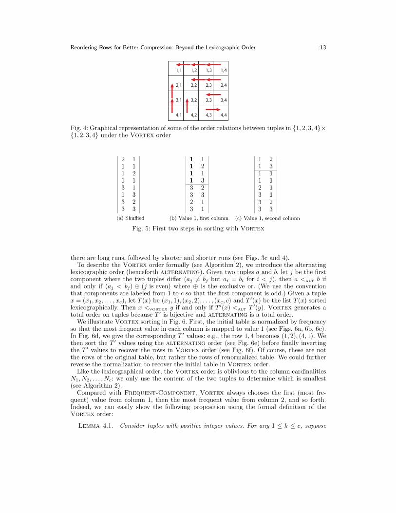
Many orders, such as z-orders with Gray codes [Faloutsos 1986] (see Fig. 3d) and Hilbertorders [Hamilton and Rau-Chaplin 2008; Kamel and Faloutsos 1994; Eavis and Cueva 2007](see Fig. 3e), use some form of bit interleaving : when comparing two tuples, we begin bycomparing the most significant bits of their values before considering the less significantbits. Our novel Vortex order interleaves individual column values instead (see Fig. 3c).Informally, we describe the order as follows:

— Pick a most frequent value x(1) from the first column, select all tuples having the valuex(1) as their first component, and put them first (see Fig. 5b with x(1) = 1);

— Consider the second column. Pick a most frequent value y(1). Among the tuples havingx(1) as their first component, select all tuples having y(1) as their second component andput them last. Among the remaining tuples, select all tuples having y(1) as their secondcomponent, and put them first (see Fig. 5c with y(1) = 1);

— Repeat.

Our intuition is that, compared to bit interleaving, this form of interleaving is more likelyto generate runs of identical values. The name Vortex comes from the fact that initially


1,21,1 1,3 1,4

2,1

3,1

4,1

2,32,2 2,4

3,2

4,2

3,3 3,4

4,3 4,4

Fig. 4: Graphical representation of some of the order relations between tuples in {1, 2, 3, 4}×{1, 2, 3, 4} under the Vortex order

2 11 11 21 13 11 33 23 3

(a) Shuffled

1 11 21 11 33 23 32 13 1

(b) Value 1, first column

1 21 31 11 12 13 13 23 3

(c) Value 1, second column

Fig. 5: First two steps in sorting with Vortex

there are long runs, followed by shorter and shorter runs (see Figs. 3c and 4).To describe the Vortex order formally (see Algorithm 2), we introduce the alternating

lexicographic order (henceforth alternating). Given two tuples a and b, let j be the firstcomponent where the two tuples differ (aj 6= bj but ai = bi for i < j), then a <ALT b ifand only if (aj < bj) ⊕ (j is even) where ⊕ is the exclusive or. (We use the conventionthat components are labeled from 1 to c so that the first component is odd.) Given a tuplex = (x1, x2, . . . , xc), let T (x) be (x1, 1), (x2, 2), . . . , (xc, c) and T ′(x) be the list T (x) sortedlexicographically. Then x <VORTEX y if and only if T ′(x) <ALT T

′(y). Vortex generates atotal order on tuples because T ′ is bijective and alternating is a total order.

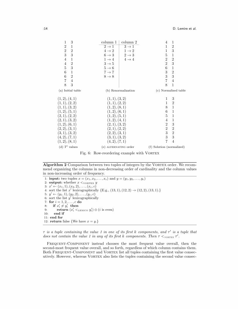
We illustrate Vortex sorting in Fig. 6. First, the initial table is normalized by frequencyso that the most frequent value in each column is mapped to value 1 (see Figs. 6a, 6b, 6c).In Fig. 6d, we give the corresponding T ′ values: e.g., the row 1, 4 becomes (1, 2), (4, 1). Wethen sort the T ′ values using the alternating order (see Fig. 6e) before finally invertingthe T ′ values to recover the rows in Vortex order (see Fig. 6f). Of course, these are notthe rows of the original table, but rather the rows of renormalized table. We could furtherreverse the normalization to recover the initial table in Vortex order.

Like the lexicographical order, the Vortex order is oblivious to the column cardinalitiesN1, N2, . . . , Nc: we only use the content of the two tuples to determine which is smallest(see Algorithm 2).

Compared with Frequent-Component, Vortex always chooses the first (most fre-quent) value from column 1, then the most frequent value from column 2, and so forth.Indeed, we can easily show the following proposition using the formal definition of theVortex order:

Lemma 4.1. Consider tuples with positive integer values. For any 1 ≤ k ≤ c, suppose


1 32 12 23 34 14 25 36 16 27 48 3

(a) Initial table

column 1 column 22→ 1 3→ 14→ 2 1→ 26→ 3 2→ 31→ 4 4→ 43→ 55→ 67→ 78→ 8

(b) Renormalization

4 11 21 35 12 22 36 13 23 37 48 1

(c) Normalized table

(1, 2), (4, 1)(1, 1), (2, 2)(1, 1), (3, 2)(1, 2), (5, 1)(2, 1), (2, 2)(2, 1), (3, 2)(1, 2), (6, 1)(2, 2), (3, 1)(3, 1), (3, 2)(4, 2), (7, 1)(1, 2), (8, 1)

(d) T ′ values

(1, 1), (3, 2)(1, 1), (2, 2)(1, 2), (8, 1)(1, 2), (6, 1)(1, 2), (5, 1)(1, 2), (4, 1)(2, 1), (3, 2)(2, 1), (2, 2)(2, 2), (3, 1)(3, 1), (3, 2)(4, 2), (7, 1)

(e) alternating order

1 31 28 16 15 14 12 32 23 23 37 4

(f) Solution (normalized)

Fig. 6: Row-reordering example with Vortex

Algorithm 2 Comparison between two tuples of integers by the Vortex order. We recom-mend organizing the columns in non-decreasing order of cardinality and the column valuesin non-increasing order of frequency.

1: input: two tuples x = (x1, x2, . . . , xc) and y = (y1, y2, . . . , yc)2: output: whether x <VORTEX y3: x′ ← (x1, 1), (x2, 2), . . . , (xc, c)4: sort the list x′ lexicographically {E.g., (13, 1), (12, 2)→ (12, 2), (13, 1).}5: y′ ← (y1, 1), (y2, 2), . . . , (yc, c)6: sort the list y′ lexicographically7: for i = 1, 2, . . . , c do8: if x′i 6= y′i then9: return (x′i <LEXICO y′i)⊕ (i is even)10: end if11: end for12: return false {We have x = y.}

τ is a tuple containing the value 1 in one of its first k components, and τ ′ is a tuple thatdoes not contain the value 1 in any of its first k components. Then τ <VORTEX τ

′.

Frequent-Component instead chooses the most frequent value overall, then thesecond-most frequent value overall, and so forth, regardless of which column contains them.Both Frequent-Component and Vortex list all tuples containing the first value consec-utively. However, whereas Vortex also lists the tuples containing the second value consec-


utively, Frequent-Component may fail to do so. Thus, we expect Vortex to producefewer runs among the most frequent values, compared to Frequent-Component.

Whereas the Hilbert order is only a Gray code when N is a power of two, we wantto show that Vortex is always an N -ary Gray code. That is, sorting all of the tuplesin {1, 2, . . . , N} × · · · × {1, 2, . . . , N} = {1, 2, . . . , N}c creates a Gray code—the Hammingdistance of successive tuples is one. We believe that of all possible orders, we might as wellpick those with the Gray-code property, everything else being equal.

Let Vortex(N1, N2, . . . , Nc) be the∏c

i=1Ni tuples in {1, 2, . . . , N1}×· · ·×{1, 2, . . . , Nc}sorted in the Vortex order. Let

ΛNc,k = Vortex(N,N, . . . , N︸︷︷︸

c−k

, N − 1, N − 1, . . . , N − 1︸︷︷︸k

).

We begin by the following technical lemmata which allow us to prove that Vortex is aGray code by induction.

Lemma 4.2. If ΛNc−1,k−1 and ΛN

c,k are Gray codes, then so is ΛNc,k−1 for any integers

N > 1, c ≥ 2, k ∈ {1, . . . , c}.Proof. Assume that ΛN

c−1,k and ΛNc,k are Gray codes. The ΛN

c,k−1 tuples begin with thetuple

(1, N, . . . , N︸︷︷︸c−k

, N − 1, N − 1, . . . , N − 1︸︷︷︸k−1

)

and they continue up to the tuple

(1, 1, N, . . . , N︸︷︷︸c−k−1

, N − 1, N − 1, . . . , N − 1︸︷︷︸k−1

).

Except for the first column which has a fixed value (one), these tuples are in reverse ΛNc−1,k−1

order, so they form a Gray code. The next tuple in ΛNc,k−1 is

(N, 1, N, . . . , N︸︷︷︸c−k−1

, N − 1, N − 1, . . . , N − 1︸︷︷︸k−1

)

and the following tuples are in an order equivalent to ΛNc,k, except that we must consider

the first column as the last and decrement its values by one, while the second column isconsidered the first, the third column the second, and so on. The proof concludes.

Lemma 4.3. For all c ≥ 1 and all k ∈ {0, 1, . . . , c}, Λ2c,k is a Gray code.

Proof. We have that Λ2c,0 is a reflected Gray code with column values 1 and 2: e.g., for

c = 3, we have the order

Λ23,0 =

1, 2, 21, 2, 11, 1, 11, 1, 22, 1, 22, 1, 12, 2, 12, 2, 2

.

Thus, we have that Λ2c,0 is always a Gray code. Any column with cardinality one can be

trivially discarded. Hence, we have that Λ2c,k is always a Gray code for all k ∈ {0, 1, . . . , c},

proving the lemma.


c = 1 c = 2 · · · CN = 2 Lemma 4.3N = 3

Lem

ma

4.4 → →

......

...

N → →Fig. 7: Illustration of the basis for the induction argument in the proof of Proposition 4.5

Lemma 4.4. For any value of N and for k = 0 or k = 1, ΛN1,k is a Gray code.

Proof. We have that ΛN1,0 is a Gray code for any value of N because one-component

tuples are always Gray codes. It immediately follows that ΛN1,1 is also a Gray code for any

N since, by definition, ΛN1,1 = ΛN−1

1,0 .

Proposition 4.5. The Vortex order is an N -ary Gray code.

Proof. The proof uses a multiple induction argument, which we express as pseudocode.At the end of each pass through the loop on N , we have that ΛN ′

c,k is a Gray code for all

N ′ ≤ N , all c ∈ {2, . . . , C} and all k ∈ {0, 1, 2, . . . , c}. The induction begins from the caseswhere there are only two values per column (N = 2, see Lemma 4.3) or only one column(c = 1, Lemma 4.4). See Fig. 7 for an illustration.

1: for N = 3, 4, . . . ,N do2: We have that ΛN−1

c,k is a Gray code for all c ∈ {2, 3, . . . , C} and also for all

k ∈ {0, 1, 2, . . . , c}. {For N > 3, this is true from the previous pass in the loopon N . For N = 3, it follows from Lemma 4.3.}

3: for c = 2, . . . , C do4: By line 2, ΛN−1

c,0 is a Gray code, and by definition ΛNc,c = ΛN−1

c,0 .5: for k = c, c− 1, . . . , 1 do6: (1) ΛN

c,k is a Gray code {when k = c it follows by line 4 and otherwise byline 8 from the previous pass of the loop on k}

7: (2) ΛNc−1,k−1 is a Gray code {when c = 2, it follows by Lemma 4.4, and for

c > 2 it follows from the previous pass of the loop on c}8: (1) + (2) ⇒ ΛN

c,k−1 is a Gray code by Lemma 4.2.9: end for10: Hence, ΛN

c,0 is a Gray code. (And also ΛNc,k for all k ∈ {0, 1, 2, . . . , c− 1}.)

11: end for12: end for

The integers N and C can be arbitrarily large. Thus, the pseudocode shows that ΛNc,k is

always a Gray code which proves that Vortex is an N -ary Gray code for any number ofcolumns and any value of N .

5. EXPERIMENTS: TSP AND SYNTHETIC DATA

We present two groups of experiments. In this section, we use synthetic data to comparemany heuristics for minimizing RunCount. Because the minimization of RunCountreduces to the TSP over the Hamming distance, we effectively assess TSP heuristics.Two heuristics stand out, and then in § 6 these two heuristics are assessed in more re-alistic settings with actual database compression techniques and large tables. The Javasource code necessary to reproduce our experiments is at http://code.google.com/p/rowreorderingjavalibrary/.

http://code.google.com/p/rowreorderingjavalibrary/

http://code.google.com/p/rowreorderingjavalibrary/


Table II: Relative reduction in RunCount compared to lexicographical sort (set at 1.0),for Zipfian tables (c = 4)

relative RunCount reductionn =8 192 n =131 072 n = 1 048 576

Lexicographic Sort 1.000 1.000 1.00Multiple Lists 1.167 1.188 1.204Vortex 1.154 1.186 1.203Frequent-Component 1.151 1.186 1.203Nearest Neighbor 1.223 1.242Savings 1.225 1.243Multiple Fragment 1.219 1.232Farthest Insertion 1.187Nearest Insertion 1.214Random Insertion 1.201Lexicographic Sort+1-reinsertion 1.171Vortex+1-reinsertion 1.193Frequent-Component+1-reinsertion 1.191

The aHDO scheme runs a complete pass through the table, trying to permute successiverows. If a pair of rows is permuted, we run through another pass over the entire table. Werepeat until no improvement is possible. In contrast, the more expensive tour-improvementheuristics (BruteForcePeephole and 1-reinsertion) do a single pass through the table.The BruteForcePeephole is applied on successive blocks of 8 rows.

5.1. Reducing the number of runs on Zipfian tables

Zipfian distributions are commonly used [Eavis and Cueva 2007; Houkjær et al. 2006; Grayet al. 1994] to model value distributions in databases: within a column, the frequency ofthe ith value is proportional to 1/i. If a table has n rows, we allow each column to haven possible distinct values, not all of which will usually appear. We generated tables with8 192–1 048 576 rows, using four Zipfian-distributed columns that were generated indepen-dently. Applying Lemma 3.1 to these tables, the lexicographical order is ω-optimal forω ≈ 3.

The RunCount results are presented in Table II. We present relative RunCount reduc-tion values: a value of 1.2 means that the heuristic is 20% better than lexicographic sort.For some less scalable heuristics, we only give results for small tables. Moreover, we omitresults for aHDO [Malik and Kender 2007] and BruteForcePeephole (with partitions ofeight rows) because these tour-improvement heuristics failed to improve any tour by morethan 1%. Because BruteForcePeephole fails, we conclude that all heuristics we considerare “locally almost optimal” because you cannot improve them appreciably by optimizingsubsets of 8 consecutive rows.

Both Frequent-Component and Vortex are better than the lexicographic order.The Multiple Lists heuristic is even better but slower. Other heuristics such as NearestNeighbor, Savings, Multiple Fragment and the insertion heuristics are even better,but with worse running time complexity. For all heuristics, the run-reduction efficiencygrows with the number of rows.

5.2. Reducing the number of runs on uniformly distributed tables

We also ran experiments using uniformly distributed tables, generating n-row tables whereeach column has n possible values. Any value within the table can take one of n distinctvalues with probability 1/n.5 For these tables, the lexicographical order is 3.6-optimal ac-

5We abuse the terminology slightly by referring to these tables as uniformly distributed: the models usedto generate the tables are uniformly distributed, but the data of the generated tables may not have uniform


Table III: Relative reduction in RunCount compared to lexicographical sort (set at 1.0),for uniformly distributed tables (c = 4)

relative RunCount reductionn =8 192 n =131 072 n = 1 048 576

Lexicographic Sort 1.000 1.000 1.00Multiple Lists 1.127 1.128 1.128Vortex 1.020 1.020 1.021Frequent-Component 1.022 1.023 1.023Nearest Neighbor 1.122 1.123Savings 1.122 1.123Multiple Fragment 1.133 1.133Farthest Insertion 1.075Nearest Insertion 1.129Random Insertion 1.103Lexicographic Sort+1-reinsertion 1.092Vortex+1-reinsertion 1.094Frequent-Component+1-reinsertion 1.080

cording to Lemma 3.1.Table III summarizes the results. The most striking difference with Zipfian tables is

that the efficiency of most heuristics drops drastically. Whereas Vortex and Frequent-Component are 20% superior to the lexicographical order on Zipfian data, they are barelybetter (2%) on uniformly distributed data. Moreover, we fail to see improved gains as thetables grow larger—unlike the Zipfian case. Intuitively, a uniform model implies that thereare fewer opportunities to create long runs of identical values in several columns, whencompared to a Zipfian model. This probably explains the poor performance of Vortex andFrequent-Component.

We were surprised by how well Multiple Lists performed on uniformly distributeddata, even for small n. It fared better than most heuristics, including Nearest Neighbor,by beating lexicographic sort by 13%. Since Multiple Lists is a variant of the greedyNearest Neighbor that considers a subset of the possible neighbors, we see that morechoice does not necessarily give better results. Multiple Lists is a good choice for thisproblem.

5.3. Discussion

For these in-memory synthetic data sets, we find that the good heuristics to minimizeRunCount—that is, to solve the TSP under the Hamming distance—are Vortex andMultiple Lists. They are both reasonably scalable in the number of rows (O(n log n))and they perform well as TSP heuristics.

Frequent-Component would be another worthy alternative, but it is harder to imple-ment as efficiently as Vortex. Similarly, we found that Savings and Multiple Fragmentcould be superior TSP heuristics for Zipfian and uniformly distributed tables, but they scalepoorly with respect to the number of rows: they have a quadratic running time (O(n2)).For small tables (n = 131 072), they were three and four orders of magnitude slower thanMultiple Lists in our tests.

6. EXPERIMENTS WITH REALISTIC TABLES

Minimizing RunCount on synthetic data might have theoretical appeal and be some-what applicable to many applications. However, we also want to determine whether row-reordering heuristics can specifically improve table compression, and therefore databaseperformance, on realistic examples. This requires that we move from general models such

histograms.


as RunCount to size measurements based on specific database-compression techniques. Italso requires large real data sets.

6.1. Realistic column storage

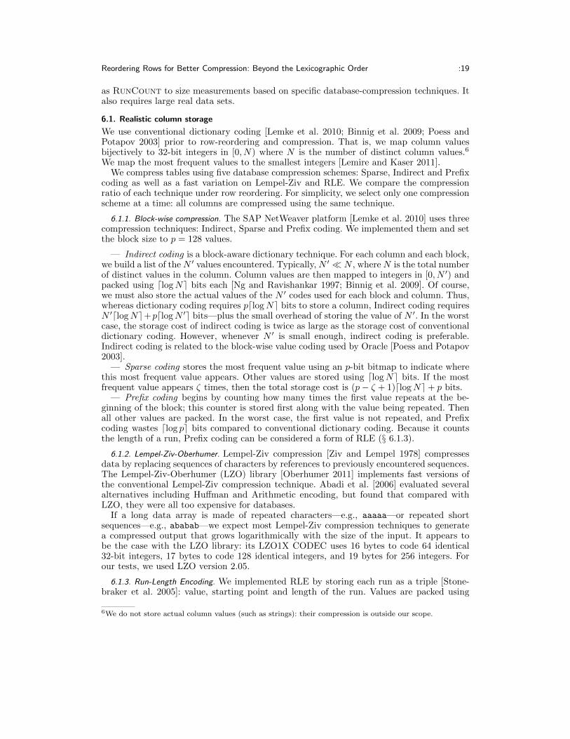
We use conventional dictionary coding [Lemke et al. 2010; Binnig et al. 2009; Poess andPotapov 2003] prior to row-reordering and compression. That is, we map column valuesbijectively to 32-bit integers in [0, N) where N is the number of distinct column values.6

We map the most frequent values to the smallest integers [Lemire and Kaser 2011].We compress tables using five database compression schemes: Sparse, Indirect and Prefix

coding as well as a fast variation on Lempel-Ziv and RLE. We compare the compressionratio of each technique under row reordering. For simplicity, we select only one compressionscheme at a time: all columns are compressed using the same technique.

6.1.1. Block-wise compression. The SAP NetWeaver platform [Lemke et al. 2010] uses threecompression techniques: Indirect, Sparse and Prefix coding. We implemented them and setthe block size to p = 128 values.

— Indirect coding is a block-aware dictionary technique. For each column and each block,we build a list of the N ′ values encountered. Typically, N ′ � N , where N is the total numberof distinct values in the column. Column values are then mapped to integers in [0, N ′) andpacked using dlogNe bits each [Ng and Ravishankar 1997; Binnig et al. 2009]. Of course,we must also store the actual values of the N ′ codes used for each block and column. Thus,whereas dictionary coding requires pdlogNe bits to store a column, Indirect coding requiresN ′dlogNe+pdlogN ′e bits—plus the small overhead of storing the value of N ′. In the worstcase, the storage cost of indirect coding is twice as large as the storage cost of conventionaldictionary coding. However, whenever N ′ is small enough, indirect coding is preferable.Indirect coding is related to the block-wise value coding used by Oracle [Poess and Potapov2003].

— Sparse coding stores the most frequent value using an p-bit bitmap to indicate wherethis most frequent value appears. Other values are stored using dlogNe bits. If the mostfrequent value appears ζ times, then the total storage cost is (p− ζ + 1)dlogNe+ p bits.

— Prefix coding begins by counting how many times the first value repeats at the be-ginning of the block; this counter is stored first along with the value being repeated. Thenall other values are packed. In the worst case, the first value is not repeated, and Prefixcoding wastes dlog pe bits compared to conventional dictionary coding. Because it countsthe length of a run, Prefix coding can be considered a form of RLE (§ 6.1.3).

6.1.2. Lempel-Ziv-Oberhumer. Lempel-Ziv compression [Ziv and Lempel 1978] compressesdata by replacing sequences of characters by references to previously encountered sequences.The Lempel-Ziv-Oberhumer (LZO) library [Oberhumer 2011] implements fast versions ofthe conventional Lempel-Ziv compression technique. Abadi et al. [2006] evaluated severalalternatives including Huffman and Arithmetic encoding, but found that compared withLZO, they were all too expensive for databases.

If a long data array is made of repeated characters—e.g., aaaaa—or repeated shortsequences—e.g., ababab—we expect most Lempel-Ziv compression techniques to generatea compressed output that grows logarithmically with the size of the input. It appears tobe the case with the LZO library: its LZO1X CODEC uses 16 bytes to code 64 identical32-bit integers, 17 bytes to code 128 identical integers, and 19 bytes for 256 integers. Forour tests, we used LZO version 2.05.

6.1.3. Run-Length Encoding. We implemented RLE by storing each run as a triple [Stone-braker et al. 2005]: value, starting point and length of the run. Values are packed using

6We do not store actual column values (such as strings): their compression is outside our scope.


Table IV: Characteristics of data sets used with bounds on the optimality of lexicographicalorder (ω), and a measure of statistical deviation (p0).

rows distinct rows cols∑

iNi ω p0Census1881 4 277 807 4 262 238 7 343 422 2.9 0.17Census-Income 199 523 196 294 42 103 419 12 0.65Wikileaks 1 178 559 1 147 059 4 10 513 1.3 0.04SSB (DBGEN) 240 012 290 240 012 290 15 8 874 195 8.0 0.10Weather 124 164 607 124 164 371 19 52 369 4.5 0.36USCensus2000 37 019 068 22 493 432 10 2 774 239 3.4 0.54

dlogNe bits whereas both the starting point and the length of the run are stored usingdlog ne bits, where n is the number of rows.

6.2. Data sets

We selected realistic data sets (see Table IV): Census1881 [Lemire and Kaser 2011; Pro-gramme de recherche en demographie historique 2009], Census-Income [Frank and Asun-cion 2010], a Wikileaks-related data set, the fact table from the Star Schema Benchmark(SSB) [O’Neil et al. 2009] and Weather [Hahn et al. 2004]. Census1881 comes from theCanadian census of 1881: it is over 305 MB and over 4 million records. Census-Income is thesmallest data set with 100 MB and 199 523 records. However, it has 42 columns and one col-umn has a very high relative cardinality (99 800 distinct values). The Wikileaks table wascreated from a public repository published by Google7 and it contains the non-classifiedmetadata related to leaked diplomatic cables. We extracted 4 columns: year, time, placeand descriptive code. It has 1 178 559 records. We generated the SSB fact table using a ver-sion of the DBGEN software modified by O’Neil.8 We used a scale factor of 40 to generateit: that is, we used command dbgen -s 40 -T l. It is 20 GB and includes 240 million rows.The largest non-synthetic data set (Weather) is 9 GB. It consists of 124 million surfacesynoptic weather reports from land stations for the 10-year period from December 1981through November 1991. We also extracted a table from the US Census of 2000 [US CensusBureau 2002] (henceforth USCensus2000). We used attributes 5 to 15 from summary file 3.The resulting table has 37 million rows.

The column cardinalities for Census1881 range from 138 to 152 882 and from 2 to99 800 for Census-Income. Our Wikileaks table has column cardinalities 273, 1 440, 3 935and 4 865. The SSB table has column cardinalities ranging from 1 to 6 084 386. (The facttable has a column with a single value in it: zero.) For Weather, the column cardinalitiesrange from 2 to 28 767. Attribute cardinalities for USCensus2000 vary between 130 001 to534 896.

For each data set, we give the suboptimality factor ω from Lemma 3.1 in Table IV.Wikileaks has the lowest factor (ω = 1.3) followed by Census1881 (ω = 2.9) whereasCensus-Income has the largest one (ω = 12.4). Correspondingly, Wikileaks and Census1881have the fewest columns (4 and 7), and Census-Income has the most (42).

We also provide a simple measure of the statistical dispersion of the frequency of thevalues. For column i, we find a most frequent value vi, and we determine what fraction of thiscolumn’s values are vi. Averaging the fractions, we have our measure p0 =

∑ci=1 f(vi)/nc,

where our table has n rows and c columns and f(vi) is the number of times vi occurs in itscolumn. As an example, consider the table in Fig. 1a. In the first column, the value ‘6’ is amost frequent value and it appears twice in 11 tuples. In the second column, the value ‘3’ ismost frequent, and it appears 4 times. In this example, we have p0 = 2+4

2×11 ≈ 0.27. In general,

7http://www.google.com/fusiontables/DataSource?dsrcid=2244538http://www.cs.umb.edu/~poneil/publist.html

http://www.google.com/fusiontables/DataSource?dsrcid=224453

http://www.cs.umb.edu/~poneil/publist.html


0

10

20

30

40

50

60

70

80

1 32 1024 32768 1048576

tim

e (m

in)

partition size (rows)

(a) Running time

0

100

200

300

400

500

600

700

800

1 32 1024 32768 1048576

com

pre

ssed

siz

e (M

B)

partition size (rows)

LZORLE

(b) Compressed data size

Fig. 8: The Multiple Lists heuristic applied on each partition of a lexicographicallysorted Weather table for various partition sizes. When partitions have size 1, we recover thelexicographical order. We refer to the case where the partition size is set to 131 072 rows asMultiple Lists? (indicated by a dashed vertical line in the plots).

we have that p0 ranges between 0 and 1. For uniformly distributed tables having highcardinality columns, the fraction p0 is near zero. When there is high statistical dispersionof the frequencies, we expect that the most frequent values have high frequencies and sop0 could be close to 1. One benefit of this measure is that it can be computed efficiently.By this measure, we have the highest statistical dispersion in Census-Income, Weather andUSCensus2000.

6.3. Implementation

Because we must be able to process large files in a reasonable time, we selected Vortexas one promising row-reordering heuristic. We implemented Vortex in memory-consciousmanner: intermediate tuples required for a comparison between rows are repeatedly builton-the-fly.

Prior to sorting lexicographically, we reorder columns in order of non-decreasing cardi-nality [Lemire and Kaser 2011]: in all cases this was preferable to ordering the columns indecreasing cardinality. For Vortex, in all cases, there was no significant difference (< 1%)between ordering the columns in increasing or decreasing order of cardinality. Effectively,Vortex does not favor a particular column order. (A related property can be formallyproved [Lemire et al. 2012].)

We used Multiple Lists on partitions of a lexicographically sorted table (see § 3.3).9

Fig. 8 shows the effect of the partition size on both the running time and the data com-pression. Though larger partitions may improve compression, they also require more time.As a default, we chose partitions of 131 072 rows. Henceforth, we refer to this heuristic asMultiple Lists?.

We compiled our C++ software under GNU GCC 4.5.2 using the -O3 flag. The C++source code is at http://code.google.com/p/rowreorderingcpplibrary/. We ran ourexperiments on an Intel Core i7 2600 processor with 16 GB of RAM using Linux. All datawas stored on disk, before and after the compression. We used a 1 TB SATA hard drivewith an estimated sustained reading speed of 115 MB/s. We used an external-memory sortthat we implemented in the conventional manner [Knuth 1997]: we load partitions of rows,

9When reporting the running time, we include the time required to sort the table lexicographically.

http://code.google.com/p/rowreorderingcpplibrary/


Table V: Compression ratio compared to lexicographical sort

Vortex Multiple Lists?

Sparse 1.27 1.00Indirect 1.07 1.02Prefix 1.45 0.99LZO 0.99 1.07RLE 1.02 1.13RunCount 0.99 1.13

(a) Census 1881


1.00 0.991.03 0.961.15 0.950.97 1.040.97 1.240.96 1.25

(b) Census-Income



(c) Wikileaks


1.00 0.991.00 0.991.00 0.971.00 1.001.00 1.001.00 1.00

(d) SSB (DBGEN)



(e) Weather


1.09 1.001.72 1.061.81 1.080.26 0.943.08 1.153.04 1.15

(f) USCensus2000

which we sort in RAM and write back in the file; we then merge these sorted partitionsusing a priority queue. Our code is sequential.

Our algorithms are scalable. Indeed, both Vortex and lexicographical sorting rely onthe standard external-memory sorting algorithm. The only difference between Vortex andlexicographical sort is that the function used to compare tuples is different. This differencedoes not affect scalability with respect to the number of tuples even though it makes Vortexslower. As for Multiple Lists?, it relies on external-memory sorting and the repeatedapplication of Multiple Lists on fixed-sized blocks—both of which are scalable.

6.4. Experimental results on realistic data sets

We present the results in Table V, giving the compression ratio on top of the lexicographicalorder: e.g., a value of two indicates that the compression ratio is twice as large as what weget with the lexicographical order.

Neither Vortex nor Multiple Lists? was able to improve the compression ratio on theSSB data set. In fact, there was no change (within 1%) when replacing the lexicographicalorder with Vortex. And Multiple Lists? made things slightly worse (by 3%) for Prefixcoding, but left other compression ratios unaffected (within 1%). To interpret this result,consider that, while widely used, the DBGEN tool still generates synthetic data. For ex-ample, out of 17 columns, seven have almost perfectly uniform histograms. Yet “real worlddata is not uniformly distributed” [Poess and Potapov 2003].

For Census1881, the most remarkable result is that Vortex was able to improvethe compression under Sparse or Prefix coding by 27% and 45%. For Census-Income,Multiple Lists? was able to improve RLE compression by 25%. For Wikileaks, wefound it interesting that Multiple Lists? reduced RunCount (and the RLE output)


Table VI: Time necessary to reorder the rows

Lexico. Vortex Multiple Lists?

Census1881 2.7 s 14 s 19 sCensus-Income 0.19 s 4.7 s 11 sWikileaks 0.3 s 2.0 s 2.5 sSSB 12 min 35 min 52 minSSB ×2.5 49 min 105 min 154 minWeather 6 min 26 min 43 minUSCensus2000 33 s 3 min 12 min

by 14% whereas the lexicographical order is already 1.26-optimal, which means thatMultiple Lists? is 1.1-optimal in this case. On Weather, the performance of Vortexwas disappointing: it worsened the compression in all cases. However, Multiple Lists?

had excellent results: it doubled the Lempel-Ziv (LZO) compression, and it improvedRLE compression by 70%. Yet on the USCensus2000 data set, Vortex was preferable toMultiple Lists? for all compression schemes except LZO. We know that the lexicographi-cal order is 3.4-optimal at reducing RunCount, yet Vortex is able to reduce RunCountby a factor of 3 compared to the lexicographical order. It follows that Vortex is 1.1-optimalin this case.

Overall, both Vortex and Multiple Lists? can significantly improve over the lexi-cographic order when a database-compression technique is used on real data. For everydatabase-compression technique, significant improvement could be obtained by at least oneof the reordering heuristics on the real data sets. However, significant degradation couldalso be observed, and lexicographic order was best in four realistic cases (Sparse codingon Census-Income, Indirect coding on Wikileaks, Prefix coding on Weather and LZO onUSCensus2000). In § 6.5, we propose to determine, based on characteristics of the data,whether significant gains are possible on top of the lexicographical order.

6.4.1. Our row-reordering heuristics are scalable. We present wall-clock timings in Table VIto confirm our claims of scalability. For this test, we included a variation of the SSBwhere we used a scale factor of 100 instead of 40 when generating the data. That is, itis 2.5 times larger (henceforth SSB ×2.5). As expected, the lexicographical order is fastest,whereas Multiple Lists? is slower than either Vortex or the lexicographical order. Onthe largest data set (SSB), Vortex and Multiple Lists? were 3 and 4 times slower thanlexicographical sorting. One of the benefits of an approach based on partitions, such asMultiple Lists?, is that one might stop early if benefits are not apparent after a fewpartitions. When comparing SSB and SSB ×2.5, we see that the running time grew by afactor of 4 for the lexicographical order, a factor of 2 for Vortex and a factor of 3 forMultiple Lists?. For SSB ×2.5, the running time of Multiple Lists? included 50 minfor sorting the table lexicographically, and the application of Multiple Lists on blocks ofrows only took 104 min. Because Multiple Lists? uses blocks with a fixed size, its runningtime will be eventually dominated by the time required to sort the table lexicographicallyas we increase the number of tuples.

6.4.2. Better compression improves speed. Everything else being equal, if less data needs tobe loaded from RAM and disk to the CPU, speed is improved. It remains to assess whetherimproved compression can translate into better speed in practice. Thus, we evaluated howfast we could uncompress all of the columns back into the original 32-bit dictionary values.Our test was to retrieve the data from disk (with buffering) and store it back on disk. Wereport the ratio of the decompression time with lexicographical sorting over the decompres-sion time with alternative row reordering methods. Because the time required to write thedecompressed values would have been unaffected by the compression, we would not expectspeed gains exceeding 50% with better compression in this kind of test.


— First, we look at our good compression results on the Weather data set withMultiple Lists? for the LZO and RLE (resp. 1.96 and 1.69 compression gain). Thedecompression speed was improved respectively by a factor of 1.19 and 1.14.

— Second, we consider the USCensus2000 table, where Vortex improved both Prefix cod-ing and RLE compression (resp. 1.81 and 3.04 compression gain). We saw gains to thedecompression speed of 1.04 and 1.12.

These speed gains were on top of the gains already achieved by lexicographical sorting. Forexample, Prefix coding was only improved by 4% compared to the lexicographical order onthe USCensus2000 table, but if we compute ratios with respect to a shuffled table, they wentfrom 1.25 for lexicographical sorting to 1.30 with Vortex. Hence, the total performancegain due to row reordering is 30%.

6.5. Guidance on selecting the row-reordering heuristic

It is difficult to determine which row-reordering heuristic is best given a table and a compres-sion scheme. Our processing techniques are already fast, and useful guidance would needto be obtained faster—probably limiting us to decisions using summaries such as thosemaintained by the DBMS. And such concise summaries might be insufficient:

— Suppose that we are given a set of columns and complete knowledge of their his-tograms. That is, we have the list of attribute values and their frequencies. Unfortunately,even given all this data, we could not predict the efficiency of the row reordering techniquesreliably. Indeed, consider the USCensus2000 data set. According to Table V, Vortex im-proves RLE compression by a factor of 3 over the lexicographical order. Consider whathappened when we took the same table (USCensus2000) and randomly shuffled columns,independently. The column histograms were not changed—only the relationships betweencolumns were affected. Yet, not only did Vortex fail to improve RLE compression over thisnewly generated table, it made it much worse (from a ratio of 3.04 to 0.74). The performanceof Multiple Lists? was also adversely affected: while it slightly improves the compressionby Prefix coding (1.08) over the original USCensus2000 table, it made compression worse(0.93) over the reshuffled USCensus2000 table.

— Perhaps one might hope to predict the efficiency of row-reordering techniques by us-ing small samples, without ever sorting the entire table. There are reasons again to bepessimistic. We took a random sample of 65 536 tuples from the USCensus2000 table. Oversuch a sample, Vortex improved LZO compression by 2.5% compared to the lexicograph-ical order, whereas over the whole data set Vortex makes LZO much worse than thelexicographical order (1.025 versus 0.26). Similarly, whereas Vortex improves RLE by afactor of 3 when applied over the whole table, the gain was far more modest over our sample(1.06 versus 3.04).

However, we can offer some guidance. For compression schemes that are closely related toRunCount, such as RLE, the optimality of a lexicographic sort should be computed usingLemma 3.1. If ω ≈ 1, we can safely conclude that the lexicographical order is sufficient.

Moreover, our results on synthetic data sets (§ 5) suggest that some statistical dispersionin the frequencies of the values is necessary. Indeed, we could not improve the RunCountof tables having uniformly distributed columns even when ω were relatively large. On ourreal data sets, we got the best compression gains compared to the lexicographical order withthe Weather and USCensus2000 tables. They both have high p0 values (0.36 and 0.54).

Hence, we propose to only try better row-reordering heuristics when ω and p0 are large(e.g., ω > 3 and p0 > 0.3). Both measures can be computed efficiently.

Furthermore, when applying a scheme such as Multiple Lists on partitions of the sortedtable, it would be reasonable to stop the heuristic after a few partitions if there is nobenefit. For example, consider the Weather data and Multiple Lists?. After 20 blocks of


131 072 tuples, we have a promising gain of 1.6 for LZO and RLE, but a disappointing ratioof 0.96 for Prefix coding. That is, we have valid estimates (within 10%) of the actual gainover the whole data set after processing only 2% of the table.

7. CONCLUSION

For the TSP under the Hamming distance, lexicographical sort is an effective and natu-ral heuristic. It appears to be easier to surpass the lexicographical sort when the columnhistograms have high statistical dispersion (e.g. Zipfian distributions).

Our original question was whether engineers willing to spend extra time reordering rowscould improve the compressibility of their tables, at least by a modest amount. Our answeris positive.

— Over real data, Multiple Lists? always improved RLE compression when compared tothe lexicographical order (10% to 70% better).

— Vortex almost always improved Prefix coding compression, sometimes by a large per-centage (80%) compared to the lexicographical order.

— On one data set, Vortex improved RLE compression by a factor of 3 compared to lexi-cographical order.

As far as heuristics are concerned, we have certainly not exhausted the possibilities.Several tour-improvement heuristics used to solve the TSP [Johnson and McGeoch 1997]could be adapted for row reordering. Maybe more importantly, we could adapt the TSPheuristics using a different distance measure than the Hamming distance. For example,consider difference coding [Moffat and Stuiver 2000; Bhattacharjee et al. 2009; Anh andMoffat 2010] where the successive differences between attribute values are coded. In thiscase, we could use an inter-row distance that measures the number of bits required to codethe differences. Just as importantly, the implementations of our row-reordering heuristicsare sequential: parallel versions could be faster, especially on multicore processors.

REFERENCES

Abadi, D., Madden, S., and Ferreira, M. 2006. Integrating compression and execution in column-orienteddatabase systems. In Proceedings of the 2006 ACM SIGMOD International Conference on Managementof Data. ACM, New York, NY, USA, 671–682.

Abadi, D. J., Madden, S. R., and Hachem, N. 2008. Column-stores vs. row-stores: how different are theyreally? In Proceedings of the 2008 ACM SIGMOD International Conference on Management of Data.ACM, New York, NY, USA, 967–980.

Agarwal, S., Agrawal, R., Deshpande, P., Gupta, A., Naughton, J. F., Ramakrishnan, R., andSarawagi, S. 1996. On the computation of multidimensional aggregates. In VLDB’96, Proceedings ofthe 22nd International Conference on Very Large Data Bases. Morgan Kaufmann, San Francisco, CA,USA, 506–521.

Anantha, M., Bose, B., and AlBdaiwi, B. 2007. Mixed-radix Gray codes in Lee metric. IEEE Trans.Comput. 56, 10, 1297–1307.

Anh, V. N. and Moffat, A. 2010. Index compression using 64-bit words. Softw. Pract. Exper. 40, 2,131–147.

Antoshenkov, G. 1995. Byte-aligned bitmap compression. In Data Compression Conference (DCC’95).IEEE Computer Society, Washington, DC, USA, 476.

Aouiche, K. and Lemire, D. 2007. A comparison of five probabilistic view-size estimation techniques inOLAP. In Proceedings of the ACM 10th International Workshop on Data Warehousing and OLAP(DOLAP ’07). ACM, New York, NY, USA, 17–24.

Applegate, D., Cook, W., and Rohe, A. 2003. Chained Lin-Kernighan for large traveling salesman prob-lems. INFORMS J. Comput. 15, 1, 82–92.

Bellmore, M. and Nemhauser, G. L. 1968. The traveling salesman problem: a survey. Oper. Res. 16, 3,538–558.

Bentley, J. 1992. Fast algorithms for geometric traveling salesman problems. INFORMS J. Comput. 4, 4,387–411.


Berman, P. and Karpinski, M. 2006. 8/7-approximation algorithm for (1,2)-TSP. In Proceedings of the17th annual ACM-SIAM symposium on Discrete algorithms. ACM, New York, NY, USA, 641–648.

Bhattacharjee, B., Lim, L., Malkemus, T., Mihaila, G., Ross, K., Lau, S., McArthur, C., Toth, Z.,and Sherkat, R. 2009. Efficient index compression in DB2 LUW. Proc. VLDB Endow. 2, 2, 1462–1473.

Binnig, C., Hildenbrand, S., and Farber, F. 2009. Dictionary-based order-preserving string compressionfor main memory column stores. In Proceedings of the 2009 ACM SIGMOD International Conferenceon Management of Data. ACM, New York, NY, USA, 283–296.

Bruno, N. 2009. Teaching an old elephant new tricks. In Proceedings, CIDR 2009 : Fourth Biennial Con-ference on Innovative Data Systems. Asilomar, USA. electronic proceedings at https://database.cs.wisc.edu/cidr/cidr2009/cidr2009.zip, last checked 2012-07-04.

Cai, J. and Paige, R. 1995. Using multiset discrimination to solve language processing problems withouthashing. Theor. Comput. Sci. 145, 1-2, 189–228.

Cesari, G. 1996. Divide and conquer strategies for parallel TSP heuristics. Comput. Oper. Res. 23, 7,681–694.

Chakrabarti, A., Chazelle, B., Gum, B., and Lvov, A. 1999. A lower bound on the complexity ofapproximate nearest-neighbor searching on the Hamming cube. In Proceedings of the 31st annual ACMsymposium on Theory of computing. ACM, New York, NY, USA, 305–311.

Cho, D.-S. and Hong, B.-H. 2000. Optimal page ordering for region queries in static spatial databases. In11th International Conference on Database and Expert System Applications (DEXA’00), LNCS 1873.Springer, Berlin, Heidelberg, 366–375.

Christofides, N. 1976. Worst-case analysis of a new heuristic for the travelling salesman problem. Tech.Rep. 388, Graduate School of Industrial Administration, Carnegie Mellon University.

Clarke, G. and Wright, J. W. 1964. Scheduling of vehicles from a central depot to a number of deliverypoints. Oper. Res. 12, 4, 568–581.

Croes, G. A. 1958. A method for solving traveling-salesman problems. Oper. Res. 6, 6, 791–812.

Dean, T. and Boddy, M. 1988. An analysis of time-dependent planning. In Proceedings of the 7th nationalconference on artificial intelligence. AAAI, Palo Alto, California, USA, 49–54.

Ding, S., Attenberg, J., and Suel, T. 2010. Scalable techniques for document identifier assignment ininverted indexes. In Proceedings of the 19th International Conference on World Wide Web (WWW’10). ACM, New York, NY, USA, 311–320.

Eavis, T. and Cueva, D. 2007. A Hilbert space compression architecture for data warehouse environ-ments. In Data Warehousing and Knowledge Discovery (DaWaK’07) (LNCS 4654). Springer, Berlin,Heidelberg, 1–12.

Ernvall, J., Katajainen, J., and Penttonen, M. 1985. NP-completeness of the Hamming salesmanproblem. Bit 25, 1, 289–292.

Faloutsos, C. 1986. Multiattribute hashing using Gray codes. SIGMOD Rec. 15, 2, 227–238.

Frank, A. and Asuncion, A. 2010. UCI machine learning repository. http://archive.ics.uci.edu/ml(checked 2012-07-04).

Fusco, F., Stoecklin, M. P., and Vlachos, M. 2010. NET-FLi: On-the-fly compression, archiving andindexing of streaming network traffic. Proc. VLDB Endow. 3, 1382–1393.

Fusco, F., Vlachos, M., and Stoecklin, M. 2012. Real-time creation of bitmap indexes on streamingnetwork data. VLDB J. 21, 3, 287–307.

Gabow, H. N. and Tarjan, R. E. 1991. Faster scaling algorithms for general graph matching problems. J.ACM 38, 4, 815–853.

Gharan, S. O., Saberi, A., and Singh, M. 2011. A randomized rounding approach to the traveling salesmanproblem. In Proceedings of the 2011 IEEE 52nd Annual Symposium on Foundations of ComputerScience. IEEE Computer Society, Washington, DC, USA, 550–559.

Gionis, A., Indyk, P., and Motwani, R. 1999. Similarity search in high dimensions via hashing. InVLDB’99, Proceedings of the 25th International Conference on Very Large Data Bases. Morgan Kauf-mann, San Francisco, CA, USA, 518–529.

Golomb, S. W. 1966. Run-length encodings. IEEE Trans. Inf. Theory 12, 3, 399–401.

Gray, J., Sundaresan, P., Englert, S., Baclawski, K., and Weinberger, P. J. 1994. Quickly generatingbillion-record synthetic databases. SIGMOD Rec. 23, 2, 243–252.

Grigoriadis, M. D. and Kalantari, B. 1988. A new class of heuristic algorithms for weighted perfectmatching. J. ACM 35, 4, 769–776.

Hahn, C., Warren, S., and London, J. 2004. Edited synoptic cloud reports from ships and land stationsover the globe, 1982–1991. http://cdiac.ornl.gov/ftp/ndp026b/ (checked 2012-07-04).

https://database.cs.wisc.edu/cidr/cidr2009/cidr2009.zip

https://database.cs.wisc.edu/cidr/cidr2009/cidr2009.zip

http://archive.ics.uci.edu/ml

http://cdiac.ornl.gov/ftp/ndp026b/


Hamilton, C. H. and Rau-Chaplin, A. 2008. Compact Hilbert indices: Space-filling curves for domainswith unequal side lengths. Inf. Process. Lett. 105, 5, 155–163.

Helsgaun, K. 2000. An effective implementation of the Lin–Kernighan traveling salesman heuristic. Eur.J. Oper. Res. 126, 1, 106–130.

Holloway, A. L. and DeWitt, D. J. 2008. Read-optimized databases, in depth. Proc. VLDB Endow. 1, 1,502–513.

Houkjær, K., Torp, K., and Wind, R. 2006. Simple and realistic data generation. In VLDB’06, Proceedingsof the 32nd International Conference on Very Large Data Bases. ACM, New York, NY, USA, 1243–1246.

Indyk, P. and Motwani, R. 1998. Approximate nearest neighbors: towards removing the curse of dimen-sionality. In Proceedings of the 30th annual ACM symposium on Theory of computing. ACM, NewYork, NY, USA, 604–613.

Indyk, P., Motwani, R., Raghavan, P., and Vempala, S. 1997. Locality-preserving hashing in multidi-mensional spaces. In Proceedings of the 29th annual ACM symposium on Theory of computing. ACM,New York, NY, USA, 618–625.

Johnson, D. S., Krishnan, S., Chhugani, J., Kumar, S., and Venkatasubramanian, S. 2004. Com-pressing large boolean matrices using reordering techniques. In VLDB’04, Proceedings of the 30thInternational Conference on Very Large Data Bases. Morgan Kaufmann, San Francisco, CA, USA,13–23.

Johnson, D. S. and McGeoch, L. A. 1997. The traveling salesman problem: A case study. In Local Searchin Combinatorial Optimization, E. H. L. Aarts and J. K. Lenstra, Eds. John Wiley and Sons, Hoboken,NJ, USA, 215–310. http://akpublic.research.att.com/~dsj/papers/TSPchapter.pdf (Last checked2012-07-04).

Johnson, D. S. and McGeoch, L. A. 2004. Experimental analysis of heuristics for the STSP. In TheTraveling Salesman Problem and Its Variations, G. Gutin and A. P. Punnen, Eds. Springer, Berlin,Heidelberg, 369–443.

Kahng, A. and Reda, S. 2004. Match twice and stitch: a new TSP tour construction heuristic. Oper. Res.Lett. 32, 6, 499–509.

Kamel, I. and Faloutsos, C. 1994. Hilbert R-tree: An improved R-tree using fractals. In VLDB’94,Proceedings of the 20th International Conference on Very Large Data Bases. Morgan Kaufmann, SanFrancisco, CA, USA, 500–509.

Kane, D. M., Nelson, J., and Woodruff, D. P. 2010. An optimal algorithm for the distinct elementsproblem. In Proceedings of the 29th ACM SIGMOD-SIGACT-SIGART symposium on Principles ofdatabase systems. ACM, New York, NY, USA, 41–52.

Karp, R. M. 1977. Probabilistic analysis of partitioning algorithms for the traveling-salesman problem inthe plane. Math. Oper. Res. 2, 3, 209–224.

Knuth, D. E. 1997. Searching and Sorting. The Art of Computer Programming Series, vol. 3. Addison-Wesley, Reading, Massachusetts.

Knuth, D. E. 2011. Combinatorial Algorithms, Part 1. The Art of Computer Programming Series, vol. 4A.Addison-Wesley, Boston, Massachusetts.

Kushilevitz, E., Ostrovsky, R., and Rabani, Y. 1998. Efficient search for approximate nearest neighborin high dimensional spaces. In Proceedings of the 30th annual ACM symposium on Theory of computing.ACM, New York, NY, USA, 614–623.

Lam, F. and Newman, A. 2008. Traveling salesman path problems. Math. Program. 113, 1, 39–59.

Lemire, D. and Kaser, O. 2011. Reordering columns for smaller indexes. Inf. Sci. 181, 12, 2550–2570.

Lemire, D., Kaser, O., and Aouiche, K. 2010. Sorting improves word-aligned bitmap indexes. Data Knowl.Eng. 69, 1, 3–28.

Lemire, D., Kaser, O., and Gutarra, E. 2012. Reordering rows for better compression: Beyond thelexicographical order. Tech. Rep. TR-12-001, UNBSJ CSAS. July.

Lemke, C., Sattler, K.-U., Faerber, F., and Zeier, A. 2010. Speeding up queries in column stores. InData Warehousing and Knowledge Discovery (DaWaK’10) (LNCS 6263). Springer, Berlin, Heidelberg,117–129.

Lin, S. and Kernighan, B. W. 1973. An effective heuristic algorithm for the traveling-salesman problem.Oper. Res. 21, 2, 498–516.

Liu, D. 2004. A strong lower bound for approximate nearest neighbor searching. Inf. Process. Lett. 92, 1,23–29.

Malik, H. H. and Kender, J. R. 2007. Optimizing frequency queries for data mining applications. InProceedings of the 7th IEEE International Conference on Data Mining (ICDM 2007). IEEE Computer

http://akpublic.research.att.com/~dsj/papers/TSPchapter.pdf


Society, Washington, DC, USA, 595–600.

Moffat, A. and Stuiver, L. 2000. Binary interpolative coding for effective index compression. Inform.Retr. 3, 1, 25–47.

Ng, W. and Ravishankar, C. 1997. Block-oriented compression techniques for large statistical databases.IEEE Trans. Knowl. Data Eng. 9, 2, 314–328.

Oberhumer, M. F. X. J. 2011. LZO real-time data compression library. online: http://www.oberhumer.com/opensource/lzo/. checked 2012-04-18.

Olken, F. and Rotem, D. 1986. Rearranging data to maximize the efficiency of compression. In Proceedingsof the 5th ACM SIGACT-SIGMOD-SIGART symposium on Principles of database systems. ACM, NewYork, NY, USA, 78–90.

O’Neil, P., O’Neil, E., Chen, X., and Revilak, S. 2009. The star schema benchmark and augmentedfact table indexing. In Performance Evaluation and Benchmarking (LNCS 5895). Springer, Berlin,Heidelberg, 237–252.

Pinar, A. and Heath, M. T. 1999. Improving performance of sparse matrix-vector multiplication. InProceedings of the 1999 ACM/IEEE conference on Supercomputing. ACM, New York, NY, USA. ArticleNo. 30.

Pinar, A., Tao, T., and Ferhatosmanoglu, H. 2005. Compressing bitmap indices by data reorganization.In Proceedings of the 21st International Conference on Data Engineering (ICDE’05). IEEE ComputerSociety, Washington, DC, USA, 310–321.

Platzman, L. and Bartholdi, III, J. 1989. Spacefilling curves and the planar travelling salesman problem.J. ACM 36, 4, 719–737.

Poess, M. and Potapov, D. 2003. Data compression in Oracle. In VLDB’03, Proceedings of the 29thInternational Conference on Very Large Data Bases. Morgan Kaufmann, San Francisco, CA, USA,937–947.

Pourabbas, E., Shoshani, A., and Wu, K. 2012. Minimizing index size by reordering rows and columns.In SSDBM’08: Proceedings of the 24th International Conference on Scientific and Statistical DatabaseManagement. Springer, Berlin, Heidelberg, 467–484.

Programme de recherche en demographie historique. 2009. The 1852 and 1881 historical censuses ofCanada. http://www.prdh.umontreal.ca/census/en/main.aspx. last checked 2012-07-04.

Reinelt, G. 1994. The traveling salesman: computational solutions for TSP applications. Springer-Verlag,Berlin, Heidelberg.

Richards, D. 1986. Data compression and Gray-code sorting. Inf. Process. Lett. 22, 4, 201–205.

Rosenkrantz, D., Stearns, R., and Lewis, II, P. 1977. An analysis of several heuristics for the travelingsalesman problem. SIAM J. Comput. 6, 3, 563–581.

Schaller, M. 1999. Reclustering of high energy physics data. In SSDBM’99: Proceedings of the 11thInternational Conference on Scientific and Statistical Database Management. IEEE Computer Society,Washington, DC, USA.

Scholer, F., Williams, H., Yiannis, J., and Zobel, J. 2002. Compression of inverted indexes for fastquery evaluation. In Proceedings of the 25th annual international ACM SIGIR conference on Researchand development in information retrieval. ACM, New York, NY, USA, 222–229.

Stonebraker, M., Abadi, D. J., Batkin, A., Chen, X., Cherniack, M., Ferreira, M., Lau, E., Lin, A.,Madden, S., O’Neil, E., O’Neil, P., Rasin, A., Tran, N., and Zdonik, S. 2005. C-Store: a column-oriented DBMS. In VLDB’05, Proceedings of the 31st International Conference on Very Large DataBases. ACM, New York, NY, USA, 553–564.

Trevisan, L. 1997. When Hamming meets Euclid: the approximability of geometric TSP and MST. InProceedings of the 29th annual ACM symposium on Theory of computing. ACM, New York, NY, USA,21–29.

US Census Bureau. 2002. United States census 2000—summary file 3. http://www.census.gov/census2000/sumfile3.html (checked 2012-07-04).

Wu, K., Otoo, E. J., and Shoshani, A. 2006. Optimizing bitmap indices with efficient compression. ACMTrans. Database Syst. 31, 1, 1–38.

Ziv, J. and Lempel, A. 1978. Compression of individual sequences via variable-rate coding. IEEE Trans.Inf. Theory 24, 5, 530–536.

http://www.oberhumer.com/opensource/lzo/

http://www.oberhumer.com/opensource/lzo/

http://www.prdh.umontreal.ca/census/en/main.aspx

http://www.census.gov/census2000/sumfile3.html

http://www.census.gov/census2000/sumfile3.html

Reordering rows for better compression: Beyond the lexicographic order

Documents

Transcript of Reordering rows for better compression: Beyond the lexicographic order