Assessing new sensor-based volume measurement methods ...

HAL Id: hal-03212399https://hal.inrae.fr/hal-03212399

Submitted on 3 Jan 2022

HAL is a multi-disciplinary open accessarchive for the deposit and dissemination of sci-entific research documents, whether they are pub-lished or not. The documents may come fromteaching and research institutions in France orabroad, or from public or private research centers.

L’archive ouverte pluridisciplinaire HAL, estdestinée au dépôt et à la diffusion de documentsscientifiques de niveau recherche, publiés ou non,émanant des établissements d’enseignement et derecherche français ou étrangers, des laboratoirespublics ou privés.

Distributed under a Creative Commons Attribution - NonCommercial| 4.0 InternationalLicense

Assessing new sensor-based volume measurementmethods for high-throughput bulk density estimation in

the field under various soil conditionsGuillaume Coulouma, Denis Feurer, Fabrice Vinatier, Olivier Huttel

To cite this version:Guillaume Coulouma, Denis Feurer, Fabrice Vinatier, Olivier Huttel. Assessing new sensor-basedvolume measurement methods for high-throughput bulk density estimation in the field under varioussoil conditions. European Journal of Soil Science, Wiley, 2021, �10.1111/ejss.13115�. �hal-03212399�

https://hal.inrae.fr/hal-03212399

http://creativecommons.org/licenses/by-nc/4.0/



https://hal.archives-ouvertes.fr

Assessing new sensor-based volume measurement methods for high-throughput

bulk density estimation in the field under various soil conditions

Running title : new bulk density estimation in the field

COULOUMA*, G., FEURER, D., VINATIER, F., HUTTEL, O.

LISAH, Univ Montpellier, INRAE, IRD, Institut Agro, F-34060 Montpellier, France

*Corresponding Author : COULOUMA, G., [email protected]

Abstract

Soil bulk density (BD) is a key soil property in soil science. BD is measured at the scale of the soil

horizon with conventional methods : core sampling and rubber balloon. Regardless of the method,

BD measurement in the field is cumbersome and time-consuming, especially in stony soils, and

new, less invasive methods have emerged but their measurement quality needs to be compared

with conventional ones. The photogrammetric technique (SfM) consists of the reconstruction of a

given scene in 3D from multi-view photographs. The aim of the present work is to assess the SfM

as a rapid, accurate method of measuring the volume of undisturbed soil for BD measurements,

regardless of the soil depth and stone content. Ten soil horizons were investigated from various

types of soils with different soil properties, especially texture (10 to 48% of clay) and stone

content (0 to 73%). The bulk density of each horizon was measured with a reference method (core

sampling), an excavation method (rubber balloon) and two recently developed sensor-based

methods: SfM and a lightweight flash lidar. For the sensor-based methods, an automated post-

processing method was developed to reduce the human operating time. The BDs measured from

the SfM were significantly similar to those measured from core sampling. At this stage, the

lightweight flash lidar is not sufficient to measure the BD with high accuracy. Finally, we

recommend the use of SfM to measure BD regarding its robustness in varying soil conditions,

especially stony soils and we discussed the potential of the method regarding the recent advances

on its field use with smartphones.

1. Introduction

Soil bulk density (BD) is a key soil property in soil science. BD is related to soil porosity,

which strongly influences the calculation of carbon content (Goidts et al., 2009), soil available

water capacity and nutrient estimation in the soil. Al Shamary et al. (2018) classify BD

Acc

epte

d A

rticl

e

This article is protected by copyright. All rights reserved.

This article has been accepted for publication and undergone full peer review but has not been through the copyediting, typesetting, pagination and proofreading process which may lead to differences between this version and the Version of Record. Please cite this article as doi: 10.1002/ejss.13115

2

measurement methods as direct or indirect measurements. The core, excavation and clod

methods involve direct measurements of the undisturbed volume of soil samples in the field (core

and excavation) or in the laboratory (clod or excavation). Radiation methods such as gamma rays

(for example, Bertuzzi et al., 1987) rely on indirect measurements in the field and require time-

consuming calibration as well as precautions related to the radiation. Whatever the available

method, the measurement of BD is time-consuming and generally requires soil pits to be dug to

allow accurate BD measurements. Consequently, BD data are sparse in existing soil databases,

which prevent the use of these databases as, for example, inputs for carbon stock calculations

(Walter et al., 2016). Pedotransfer functions are commonly used for the prediction of BD (Qiao et

al., 2019; Chen et al., 2018) based on relationships between well-characterized soil variables (for

example, texture and organic carbon content) and bulk density measurements.

The effectiveness of conventional methods used to measure BD at the scale of the soil

horizon, such as core sampling and rubber balloon, are also limited by its stone content. The core

method is currently considered the standard method for direct BD estimation (Blake and Hartge,

1986). However, the reference core volume varies across studies and results in biases in the

measured BDs (Terry et al. 1981). Terry et al. (1981) found that smaller cores (33 cm3) enhanced

the compression effect and that larger cores (2792 cm3) captured macroporosity in the case of

forest soils without gravel or stones. Moreover, the core sampling method is not applicable

everywhere. The core sampling method is not usable in the case of stony soils or soils without

sufficient structure. Excavation methods are then an alternative. The principle of the excavation

method is based on the direct measurement in the field of the undisturbed volume with water,

sand or Styrofoam balls (Grossman and Reinsch, 2002). To prevent the loss of water due to

infiltration, different imaginative ways to seal the border of the excavation have been developed.

The rubber balloon method replaces the void spaces with a rubber balloon filled with a volume of

water directly measured on the excavation tool (Andraski et al. 1991). In the same way, Van

Remortel (1993) sealed the border of the excavation with plastic wrap. Excavation with foam

(Laundre, 1989) or plaster (Frisbie et al., 2014; Scanlan et al., 2018) is also a satisfactory method

but is even more time-consuming than the other methods. Moreover, all of the excavation

methods recommended in the case of stony soils are difficult to apply vertically (Brye et al.,2004).

Finally, the clod method consists of sampling clods within the soil horizons and measuring their

volume in the laboratory following different methods (Archimedes’ principle, X-ray tomography,

photogrammetry). The difficulties arise with disaggregation during transport and the risk of

selecting specific hard soil structure features within the soil horizon. All of these methods have

Acc

epte

d A

rticl

e


3

been compared in the literature in terms of their effectiveness and cost as well as the

representativeness of the measured BD (for example Al Shammary et al., 2018).

New developments have been made in the use of photogrammetry in terms of the number

of available platforms, sensors, and software packages (Smith et al 2015). The structure from

motion photogrammetric technique, denoted SfM hereafter, consists of the reconstruction of a

given scene in 3D from multi-view photographs. Moret-Fernandez et al. (2016), and more recently

Whiting et al. (2020) characterised the volume of small soil aggregates in the laboratory with SfM

techniques . Bauer et al. (2014) tested SfM directly in the field on eight different soil surfaces and

compared it with classical sand excavation for stony soils (4 out of 8 sites) and core methods for

the rest. The SfM estimated the volume with a better precision than the sand replacement

method. The comparison with the core method showed differences, mainly due to soil surface

cracks that were not sampled in the cores. In the same way, 3D scanning methods were applied to

BD measurement in the laboratory by Rossi et al. (2008) with a laser scanner on soil aggregates

and most recently, Bagnall et al (2020) characterised the soil structure from the pit flank with a

lidar. Scanlan et al. (2018) also used a Kinect sensor from the soil surface but with depth

increments to characterize the BD at four different depths within the same excavation. The

authors compared the volume calculated from the scanning system with the volume from a

classical plaster cast of the excavation hole. The differences were exacerbated in the deeper

measurements due to border effects. More recently, Polyakov et al. (2019) proposed terrestrial

LiDAR as an alternative to the classical excavation method in stony soils for BD measurements at

the surface with strong limitations due to the technical requirements and the cost of the device.

However, these promising techniques were only tested in horizontal situations and from

the soil surface (Bauer et al., 2014; Scanlan et al., 2018; Polyakov et al., 2019). For example, Brye

et al. (2004) already note the need to measure BD along the exposed face of soil profiles,

especially in the case of stony soils. The punctual soil investigations require a vertical approach

through the horizonation within the soil pits to obtain a large set of soil property measurements

(Hartemink and Minasny, 2014). Currently, there is a lack of study on the comparison of

conventional versus new sensor based methods in situ for a large range of soils.

Considering the need for BD data in many soil science applications, the aim of the present

work is to assess SfM as an all-terrain method capable of overcoming the limitations of

conventional methods for BD measurements, regardless of the stone content. Moreover, a simple

and inexpensive 3D sensor is simultaneously tested with photogrammetry and other classical

methods used as references: core sampling and the rubber balloon method. To the best of our

Acc

epte

d A

rticl

e


4

knowledge, our study is the first to assess and compare these four techniques on the same

horizons with investigations both from above and from the side of the pit. Starting with a brief

description of all the methods tested in the study, their associated protocols and their

corresponding operating times, we compared all combinations of methods on the basis of a

complete field dataset covering a large range of stone contents, organic carbon, textures, and

structures.

2. Material and methods

2.1. Study area The seven investigated pits that constitute the experimental dataset of this study were located in

five study areas, all included in the Langedoc (southern France). They were selected to be

representative of the diversity of soil characteristics that may change the bulk density

measurement conditions (e.g., coarse fragments, texture, soil depth) and the bulk density itself

(e.g., structure). A morphological description was performed on each pit according to the FAO

guidelines for soil description (FAO, 2006). The final ten investigated horizons were chosen among

this available different soil horizons, which is why not all the horizons at the same site were

investigated. Five soil pits were dug in January, July and October 2018 for the Pech Rouge

(43°08’33’’, 3°07’59’’), Lavalette (43°08’33’’, 3°07’59’’) and Mauguio (43°35’33’’,4°00’39’’) sites,

respectively and two additional soil pits were investigated in September 2020 for the Angles

(43°31’14’’,2°31’45’’) and Restinclieres (43°45’58’’,3°51’15’’) sites. Samples of over 500 g were

taken from each horizon for further laboratory characterization. The particle size distribution

(texture), gravel and stone content, organic carbon content (OC), and calcium carbonate content

(CaCO3) were measured at the French INRAE-ARRAS laboratory. Each sampled horizon is denoted

(Site name)_(Pit number when there were multiple pits in a site)_H(horizon number, from top to

bottom). Tables 1 and 2 summarize the characteristics of this soil dataset. Lavalette_H2,

Mauguio_2_H2, and Pech_H2 correspond to deeply tilled horizons with high structural variability.

Lavalette_H4 and Mauguio_1_H3 show medium to high porosity due to high microfaunal activity.

The clay content is highly variable between the investigated horizons, from 10% for Pech_H2 to

48% for Mauguio_3_H2. The organic carbon is generally low except in the Angles_H1 covered by

Acc

epte

d A

rticl

e


5

Douglas trees. Finally, the coarse fragment varied between low content in Mauguio_H1 to a

maximum in Mauguio_3_H2.

<Table 1 and 2 here>

2.2. Soil bulk density estimation 2.2.1 General experimental setup Each of the ten horizons was investigated both on the side of the pit (core sampling, SfM, flash

LiDAR) and from above after digging to reach the given horizon (rubber baloon, SfM, flash LiDAR).

<figure 1 here>

Investigations from the vertical side of the horizons: core sampling, SfM and Flash LiDAR

The first investigations were performed directly in the side of the pit (figure 1a) with the same

procedure repeated for each investigated soil horizon. One unique flash lidar data acquisition of

the whole horizon was performed immediately followed by an SfM acquisition that also covered

the whole horizon. Both of these procedures were done before soil sampling. Then, five

excavations were performed for each sampled horizon. Once the soil was sampled at these five

locations, a second flash lidar acquisition of the whole soil horizon and a SfM acquisition of the

whole horizon were performed after the soil sampling. Finally, three repetitions of core sampling

with 100 cm3 cores (Blacke and Hartge, 1986) were performed within each of the five excavations.

Hence, the flash lidar data and SfM acquisitions imaged exactly the same volumes, while the core

sampling method investigated its own fixed volume samples at the back of each excavation.

Investigations from the horizontal side of the horizons: rubber ballon, SfM and Flash LiDAR

For each investigated horizon, the same procedure described hereafter was used (figure 1b). First,

soil was removed to constitute a planar horizontal surface at the average level of the five

excavations previously dug from the sides of the pit in order to investigate the same zone

(previous section) of a given soil horizon. Five excavations were performed, following the

recommendation of the rubber balloon method (NF X31-502). For each excavation, exactly the

same excavated volume was measured with three methods: rubber balloon, flash lidar and SfM.

The same procedure was used as above, but with the addition of a density plate around each

Acc

epte

d A

rticl

e


6

excavation, fixed with iron fastening clips, which was necessitated by the rubber balloon

acquisition (figure 1b). Adding a density plate to the protocol necessitated moving both the

density plate and flash lidar from one excavation to another, leading to five acquisitions with each

method for a given horizon, compared to only one acquisition from the side of the pit.

The following table (Table 3) summarizes the soil samples taken for each of the ten investigated

horizons of the seven different pits.

<Table 3 here>

2.2.2 Laboratory sample processing for raw and fine bulk density estimation

The excavated samples were dried (48 h at 105°C) and weighed in the lab. Bulk densities (ρb) were

determined as the ratio between the dry soil mass and the total sampled volume. As some

samples contained high volumes of gravels and stones, we calculated a fine earth bulk density

(ρbFE) without coarse fragments. To that end, each sample was sieved to extract the coarse

fragments (e.g., >2 mm). There were different types of coarse fragments, and their density was

measured following the classical method based on the Archimede’s principle. The values varied

between 1.9 for the highly weathered pebbles in Angles_H1 to 2.6 for the limestones in

Restinclieres_H1. The ρbFE was determined as the ratio between the dry soil mass without the

coarse fragments and the total sampling volume without the volume corresponding to the coarse

fragments. This latter volume was calculated from the mean bulk density of the coarse fragments

given in table 2. Due to the large range of coarse fragments within the dataset, the ρbFE values

were chosen to compare the methods.

2.3 Sensor-based volume measurement - data acquisition

For all the investigations, a canopy was used to obtain homogeneous lighting. The canopy was

used to prevent shadowing and shade changes during sensor-based data acquisition and soil

sampling.

2.3.1. Flash lidar

Acc

epte

d A

rticl

e


7

We used a PmdTec Pico Flexx flash lidar sensor operated from a smartphone and fixed on an angle

iron so that it did not move between the before and after acquisitions. The sensor provides 224 x

171 3D frames with a given precision of 1% of the distance, which corresponds to the order of

magnitude of the centimetre in our case (acquisition at approx. one metre).

Acquisition was performed over five seconds for median temporal filtering of the point cloud to

decrease noise and eliminate outliers. For a minority of acquisitions, a small offset between the

two point clouds was observed, most likely because the angle iron may have shifted during soil

sampling. These particular point clouds were thus co-registered by using the ICP algorithm of

CloudCompare 2.10.1.

2.3.2. SfM We used a Nikon D3200 camera with an 18-55 mm AF Nikkor objective set at 18 mm with camera

focus fixed so that camera parameters could be considered constant during the acquisitions. A

convergent set of at least 20 images - both before and after soil sampling - was acquired to cover

the whole area with multi-view stereoscopic imagery, including the scale bars with coded targets.

In the office, all images taken before and after excavation were processed with the Time-SIFT

method (Feurer and Vinatier, 2018) using Agisoft Photoscan 1.2.6 to produce two 3D point clouds

with the exact same geometric reference. Coded targets were used to scale the model. For soil

samples taken from the side of the pit, a single pair of before and after point clouds was obtained

for the whole horizon. For soil samples taken from above, there was one pair of before and after

point clouds for each excavation.

2.4 Sensor-based data post-processing 2.4.1 Manual post-processing method

For the manual estimation of excavation volumes, 3D point clouds derived from flash lidar and/or

SfM acquisition were processed together in the CloudCompare 2.10.1 software. A cloud-to-cloud

distance was computed, and the 3D point clouds were coloured with this distance information.

Each excavation was then manually delineated and clipped. Finally, the excavated volume was

computed as a 2.5D volume on a 1 mm resolution grid.

2.4.2 Automatic post-processing method

Acc

epte

d A

rticl

e


8

After automatically trimming the borders of the excavations, dense 3D point clouds resulting from

the flash lidar and SfM acquisitions were processed in several steps consisting of a combination of

calls to CloudCompare 2.10.1 functions using R software and raster processes using the ‘raster’ R

library. Excavated holes were detected using cloud-to-cloud distances between 3D point cloud

before and after excavation, considering the minimal areas of the holes and the level of noises of

the methods (Figure 2). The complete method is available as an R code in the open access

repository Zenodo at the following URL (https://doi.org/10.5281/zenodo.4036423), and a sample

dataset is available at the following URL (https://doi.org/10.5281/zenodo.4036313).

<Figure 2 here>

2.5. Comparison of operating times The long operating time of core sampling is mainly due to the high number of samples required to

improve the statistical significance of the measured bulk density. The other methods require

similar, lower operating times. However, the rubber balloon method in the field is also time-

consuming compared to the sensor-based methods (Table 4).

<Table 4 here>

2.6. Statistical analyses

First, manual and automatic processing for volume estimation were compared two-by-two (SfM

and flash Lidar) using a linear model. Second, taking the automatic volume processing as the basis

for volume calculations, volumes issued from SfM method were compared to those issued from

rubber balloon and flash lidar using a linear model and the classical figures of merit (R2, RMSE,

intercept and slope) of the model as descriptors of the accuracy of the correlation between

variables. Finally, all densities calculated from the automatic volume processing were compared

using ANOVA considering the methods, horizons and replicates as explanatory variables. Reliability

of the SfM method to the others was tested using differences in means and Tukey’s HSD post hoc

criterion.

Acc

epte

d A

rticl

e


https://doi.org/10.5281/zenodo.4036423

9

3. Results

3.1 Representativity of the dataset in terms of volumes and densities

3.1.1 Range of raw density ρb

Based on the classical core sampling reference method, the studied horizons corresponded to a

large observed range of ρb [1.04 - 1.71] mainly due to their various structural arrangements,

organic carbon content and porosities. This dataset covered a large part of the bulk density

measured in national databases (for example Hollis et al., 2012). The highest ρb values measured

with core sampling were in Mauguio_1_H2, due to tillage and wheeling degradations. The highest

ρb values (a mean of 2.01, measured in Mauguio_3_H2 with flash lidar and SFM) could not be

measured with core sampling due to high pebble and gravel content (the highest : 73% in mass).

The lower ρb values corresponded to the organic horizon Angles_H1 (1.04). The ρbFE were lower

than the ρb values due to the high content of coarse fragments in some horizons.

3.1.2 Range of measured volumes

The distribution of the volumes measured with rubber balloon, SFM and flash lidar demonstrate a

large range from 100 to 1400 cm3. The high number of measurements around the median (385

cm3) corresponded to the rubber balloon excavations.

3.2. Comparison of the volume estimation from SfM, flash lidar, and rubber balloon The automatic post-processing method used to estimate the volume from sensor-based methods

was compared to the manual post-processing method. The automatically estimated volumes from

both SfM and flash lidar were extremely similar to those estimated by the manual approach

(R2=0.998, RMSE of 11 cm3). Therefore, automatic post-processing was used in the rest of the

analysis.

In the case of the investigation of the horizons from above, the excavations were sized for the

rubber balloon method, and exactly the same holes were scanned by the flash lidar and SfM.

Hence, for these samples, exactly the same volumes from the three methods were measured and

compared. The volumes measured by rubber balloon were systematically greater than the

volumes measured by SfM (intercept of the linear model = 12 cm3, P<0.05 Student’s t-test) (Figure

3a). Conversely, no bias was observed between the volumes from flash lidar and SfM (Figure 3b).

However, the relationship between the volumes was noisy, especially at larger volumes, with an

RMSE of 36 cm3.

Acc

epte

d A

rticl

e


10

<Figure 3 here >

3.3 Determination of the bulk densities at the horizon scale <Table 5 here>

A comparison between the methods was conducted on the basis of the ρbFE (figure 4 and table 5).

The ρbFE values measured from sensor-based methods were similar regardless of the soil

characteristics, except for Lavalette_H2 (Tukey’s HSD test, P<0.01). However, the standard

deviation of the flash lidar data was systematically higher than those of SFM. The significant noisy

measurement of the volume (an RMSE of 36 cm3) directly corresponds to a high standard

deviation of the resulting BD (more than 0.05 for a volume of 1000 cm3). The comparison between

classical methods and SFM showed differences in relation to the coarse fragments. For low

content of coarse fragments (i.e. <15% in mass), The ρbFE values measured from core sampling

were significantly the same of those from SFM (Tukey’s HSD test, P<0.01), except for

Mauguio_1_H3 and Mauguio_2_H2. Moreover, the standard deviations of ρbFE from both core

sampling and SfM measured within each horizon were also similar. The ρbFE values measured from

rubber balloon was systematically lower than that measured from SFM and significantly lower for

Lavalette_H2, Mauguio_3_H3, and Pech_2 (Tukey’s HSD test, P<0.01).

<figure 4 here>

Conversely for high content of coarse fragments, the ρbFE measured from core sampling were

always lower than the other methods, regardless of the other soil properties (Tables 5 and 2).

Finally, the variability of the measurements was high whatever the methods. The flash lidar

resulted to the highest standard deviation measured in the Angles_H1 horizon and Mauguio_3_H2

horizon (the highest coarse fragment content).

Acc

epte

d A

rticl

e


11

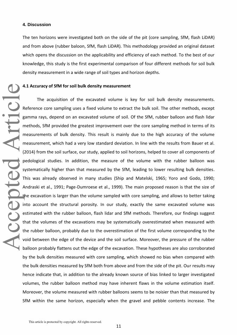
4. Discussion

The ten horizons were investigated both on the side of the pit (core sampling, SfM, flash LiDAR)

and from above (rubber baloon, SfM, flash LiDAR). This methodology provided an original dataset

which opens the discussion on the applicability and efficiency of each method. To the best of our

knowledge, this study is the first experimental comparison of four different methods for soil bulk

density measurement in a wide range of soil types and horizon depths.

4.1 Accuracy of SfM for soil bulk density measurement

The acquisition of the excavated volume is key for soil bulk density measurements.

Reference core sampling uses a fixed volume to extract the bulk soil. The other methods, except

gamma rays, depend on an excavated volume of soil. Of the SfM, rubber balloon and flash lidar

methods, SfM provided the greatest improvement over the core sampling method in terms of its

measurements of bulk density. This result is mainly due to the high accuracy of the volume

measurement, which had a very low standard deviation. In line with the results from Bauer et al.

(2014) from the soil surface, our study, applied to soil horizons, helped to cover all components of

pedological studies. In addition, the measure of the volume with the rubber balloon was

systematically higher than that measured by the SfM, leading to lower resulting bulk densities.

This was already observed in many studies (Ship and Matelski, 1965; Yoro and Godo, 1990;

Andraski et al., 1991; Page-Dumroese et al., 1999). The main proposed reason is that the size of

the excavation is larger than the volume sampled with core sampling, and allows to better taking

into account the structural porosity. In our study, exactly the same excavated volume was

estimated with the rubber balloon, flash lidar and SfM methods. Therefore, our findings suggest

that the volumes of the excavations may be systematically overestimated when measured with

the rubber balloon, probably due to the overestimation of the first volume corresponding to the

void between the edge of the device and the soil surface. Moreover, the pressure of the rubber

balloon probably flattens out the edge of the excavation. These hypotheses are also corroborated

by the bulk densities measured with core sampling, which showed no bias when compared with

the bulk densities measured by SfM both from above and from the side of the pit. Our results may

hence indicate that, in addition to the already known source of bias linked to larger investigated

volumes, the rubber balloon method may have inherent flaws in the volume estimation itself.

Moreover, the volume measured with rubber balloons seems to be noisier than that measured by

SfM within the same horizon, especially when the gravel and pebble contents increase. The

Acc

epte

d A

rticl

e


12

balloon may not truly match the edges of the excavations, although the shape follows smooth

edges during the excavation. The coarse gravels and pebbles may modify the contact between the

balloon and the excavation edge and result in an increase in noise.

Excavation methods are generally used in the literature when the gravel and stone content of the

soil exceeds 10% by mass. The different horizons tested in our study show the satisfactory

applicability of the SfM method in these cases. Indeed, the total amount of gravel and stone varied

from 0 to 73% (in mass), and the SfM method was not impacted by the gravel content. Similarly,

the rubber balloon method is not recommended in the case of sandy textures due to the collapse

of the excavation (Andraski et al., 1991). In our study, the SfM method succeeded in the sandy

Pech_H2 horizon (79% of sand). However, it must be noted that the bulk density was slightly

overestimated compared to that estimated by core sampling.

Kutilek and Nielsen (1994) discussed about the representative elementary volume (REV) in

Hydrodynamic and calculated a REV minor than 100 cm3 for poor structured soils and larger for

well-structured soils. The core sampling with a fixed investigated volume is limiting in order to

characterise structured soils. The size of the excavation for SfM measurement may be adapted to

each situation to take into account the different specific porosities (small cracks, structural vughs,

pebble size). This point was already made by Bauer et al. (2014) in the case of small soil surface

cracks that could not be characterized by classical core sampling. Scanlan et al. (2018) noted the

value of sizing the excavation to characterize different representative volumes. For example in

Mauguio_1_H3 with a high porosity combined to a very clear structure, the volume investigated

with the core sampling were lower than those from SFM and flash lidar (more than 1000 cm3) and

probably did not include the structural porosity. Consequently, the ρbFE values from core sampling

were higher than from the other methods. Finally, an additional advantage of SfM is its

applicability regardless of the orientation of the soil face, along the side of the pit or from above.

4.2 Displaying SfM from the field to the lab

In addition to the demonstrated accuracy and precision of the volume estimation both from above

and from the side of the pit, a great advantage of the proposed SfM method is the very low time

needed in the field (Table 4), as already noted in previous studies (Bauer et al., 2014; Scanlan et

al., 2018). Moreover, the volume is directly measured in the field and any undisturbed samples

need to be returned to the laboratory for fine volume measurement, as proposed SfM methods

from Moret-Fernandez et al. (2016) or from Whiting et al. (2020). Field work is often performed

under time constraints. The representativity of the sampling with only 5 samples (a total of 1500

Acc

epte

d A

rticl

e


13

cm3 on average) is at least comparable to that of the core sampling with an equivalent of 15

samples. However, the sampling must follow important recommendations mainly: (i) maintain a

smooth shape of the excavation, (ii) be careful to maintain a good lighting of the image without

potential moving objects , and (iii) prevent external soil particles from falling during the

excavation.

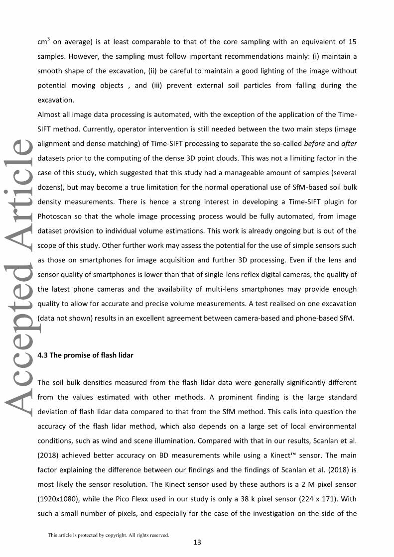
Almost all image data processing is automated, with the exception of the application of the Time-

SIFT method. Currently, operator intervention is still needed between the two main steps (image

alignment and dense matching) of Time-SIFT processing to separate the so-called before and after

datasets prior to the computing of the dense 3D point clouds. This was not a limiting factor in the

case of this study, which suggested that this study had a manageable amount of samples (several

dozens), but may become a true limitation for the normal operational use of SfM-based soil bulk

density measurements. There is hence a strong interest in developing a Time-SIFT plugin for

Photoscan so that the whole image processing process would be fully automated, from image

dataset provision to individual volume estimations. This work is already ongoing but is out of the

scope of this study. Other further work may assess the potential for the use of simple sensors such

as those on smartphones for image acquisition and further 3D processing. Even if the lens and

sensor quality of smartphones is lower than that of single-lens reflex digital cameras, the quality of

the latest phone cameras and the availability of multi-lens smartphones may provide enough

quality to allow for accurate and precise volume measurements. A test realised on one excavation

(data not shown) results in an excellent agreement between camera-based and phone-based SfM.

4.3 The promise of flash lidar

The soil bulk densities measured from the flash lidar data were generally significantly different

from the values estimated with other methods. A prominent finding is the large standard

deviation of flash lidar data compared to that from the SfM method. This calls into question the

accuracy of the flash lidar method, which also depends on a large set of local environmental

conditions, such as wind and scene illumination. Compared with that in our results, Scanlan et al.

(2018) achieved better accuracy on BD measurements while using a Kinect™ sensor. The main

factor explaining the difference between our findings and the findings of Scanlan et al. (2018) is

most likely the sensor resolution. The Kinect sensor used by these authors is a 2 M pixel sensor

(1920x1080), while the Pico Flexx used in our study is only a 38 k pixel sensor (224 x 171). With

such a small number of pixels, and especially for the case of the investigation on the side of the

Acc

epte

d A

rticl

e


14

pit, sampling of the 3D surface may not be sufficient to correctly depict the geometries before and

after excavation. On the other hand, Polyakov et al. (2019) used a professional-grade terrestrial

laser scanner whose accuracy and precision specifications are totally different from the

specifications of the lightweight flash lidar such as the ones used in the study of Scanlan et al.

(2018) and in this study. However, their work confirms the interest in using laser-based sensors for

volume measurements, and our three studies definitely demonstrate the strong potential of 3D

sensors for soil studies. Considering the differences among the sensors used in our three studies, it

is still hard to determine whether continuous flash lidar scanning (as proposed by Scanlan et al.

(2018) is needed to obtain the required precision and accuracy or whether a single point of view

with time averaging (as we propose in our study), but with a better sensor would be sufficient.

Regardless, the main advantages of using such lightweight range imaging sensors are their easy

handling without prior specific knowledge and the large frame (more than 2 m²) recorded during

just a few seconds. These devices also connect directly to a simple smartphone and do not need a

single- lens reflex camera, which is advised for the SfM. Finally, it is expected that better

lightweight flash lidar devices will become available and would allow the use of this method to

obtain the required accuracy and precision for the volume estimations.

4.4 The bulk density of fine earth from the stony soils

The studied dataset showed large differences with the measurement of bulk density in relation to

the coarse fragment contents. Core sampling was considered as a reference for the measurement

of bulk density in numerous studies. In case of low coarse fragment contents (i.e. <15%), the

sampling was possible with the core sampling and a simple correction is sufficient to study the

bulk density of the fine earth. Restinclieres_H2 and Angles_H1, with respectively 24 and 36 % in

mass of coarse fragment contents, presented lower bulk densities of the fine earth than expected

with the core sampling method. During the sampling in the field, the fine gravels and gravels were

easily included in the core stainless steel and did not significantly deflect the driving of the core.

However, the stones modified the driving and the structure of the sample. The resulting sample

consequently contained lower quantity of fine earth. Conversely, the excavation methods

undisturbed the structure of the fine earth whatever the gravel and stone content. The

comparison with the core sampling was biased and conducted to an underestimation of ρbFE with

the core sampling. In case of very high stone content (Mauguio_3_H2), the core sampling was

Acc

epte

d A

rticl

e


15

even not applicable at all. The sensor-based excavation methods denoted low and noisy ρbFE

values, which probably depend on the irregular voids between the stones.

Stony soils (i.e. soils with more than 30 % in mass of coarse fragments) represent a large part of

the Mediterranean soils and more generally of the European countries (The soil map of Europe,

2014). New studies focusing on the relation between stony soils and water retention show the

importance of stones and the relation between stones and fine earth (for example, Korboulewsky

et al. (2020)). The structural arrangements within the fine earth in stony soils needs to be studied

and the new proposed excavation methods may improve future datasets.

5. Conclusion

Although BD is a key property in soil science, the classical methods for measuring BD in the field

are time-consuming and present some limitations, especially in stony soils. The aim of the present

work was to assess SfM as an all-terrain method capable of overcoming the limitations of

conventional methods for BD measurements, regardless of the stone content. The SfM method

provides accurate measurements with significantly less time in the field than the traditional

method, regardless of the soil conditions. Moreover, the representativeness of the measurement

is larger than that of the reference core sampling and is adjustable according to the size of the

different soil porosities. The volume of excavations measured from rubber balloons, which are

often used in the case of stony soils, is significantly higher than the volume measured from the

SfM. This result confirms the bias of the rubber balloon method, which is often discussed in the

literature. At this stage, lightweight flash lidar is not sufficient to measure BD with high accuracy.

However, the flash lidar method is very accessible, and technical advances may provide more

accurate devices in the future. Finally, the authors recommend the use of SfM to measure BD.

6. Acknowledgements

This study was directly supported by the LISAH research team. The authors thank N. Saurin for his

kind help at the Pech Rouge site, the DIASCOPE team and Y. Blanca for their appreciated help at

the Mauguio site.

Conflict of interest: None

Data availability statement:

R code https://doi.org/10.5281/zenodo.4036423

Acc

epte

d A

rticl

e


16

Sample dataset https://doi.org/10.5281/zenodo.4036313

7. References

Al-Shammary, A.A.G., Kouzani, A.Z., Kaynak, A., Khoo, S.Y., Norton, M., & Gates, W. (2018). Soil

Bulk Density estimation methods: A review. Pedosphere, 28(4), 581-596.

Andraski, B.J. (1991). Balloon and core sampling for determining Bulk Density of alluvial desert soil.

Soil Science Society of America Journal, 55, 1188-1190.

Bagnall, D.K., Jones, E.J., Balke, S., Morgan, C.L.S., & McBratney, A.B. (2020). An in situ method for

quantifying tillage effects on soil structure using multistripe laser triangulation. Geoderma 380, in

press.

Bauer, T., Strauss, P., & Murer, E. (2014). A photogrammetric method for calculating soil bulk

density. Journal of Plant Nutrition and Soil Science, 177, 496-499.

Bertuzzi, P., Bruckler, L., Gabilly, Y., & Gaudu, J.C. (1987). Calibration, field testing, and error

analysis of a gamma-ray probe for in situ measurement of dry bulk density. Soil

Science, 144(6), 425-436.

Blake, G.R., Hartge, K.H., 1986. Bulk density. In: Klute, A., Ed., Methods of Soil Analysis, Part 1—

Physical and Mineralogical Methods, 2nd Edition, Agronomy Monograph 9, American

Society of Agronomy—Soil Science Society of America, Madison, 363-382.

Brye, K.R., Morris, T.L., Miller, D.M., Formica, S.J., & Van Eps, M.A. (2004). Estimating Bulk Density

in vertically exposed stoney alluvium using a modified excavation method. Journal of

Environmental Quality, 33, 1937-1942.

Chen, S., Richer-de-Forges, A.C., Saby, N.P.A., Martin, M.P., Walter, C., & Arrouays, D. (2018).

Building a pedotransfer function for soil bulk density on regional dataset and testing its

validity over a larger area. Geoderma, 312, 52-63.

FAO, 2006. Guidelines for soil description. Fourth edition. FAO, Rome

Feurer, D., & Vinatier, F. (2018). Joining multi-epoch archival aerial images in a single SfM block

allows 3-D change detection with almost exclusively image information. ISPRS Journal

of Photogrammetry and Remote Sensing, 146, 495-506.

Frisbie, J.A., Graham, R.C., & Lee, B.D. (2014). A plaster cast method for determining soil Bulk

Density. Soil Science,179, 103-106.

Acc

epte

d A

rticl

e


17

Goidts, E., van Wesemael, B., & Crucifix, M. (2009). Magnitude and sources of uncertainties in soil

organic carbon (SOC) stock assessments at various scales. European Journal of Soil

Science, 60(5), 723-739.

Grossman, R.B., & Reinsch, T.G. (2002). Bulk Density and linear extensibility, In: Dane,J.J., & Topp,

G.C., Ed., Methods of Soil Analysis, Part 4—Physical Methods, 5.4—Soil Science Society

of America, Madison, 201-228.

Hartemink, A.E., and Minasny, B. (2014). Towards digital soil morphometrics. Geoderma, 230-231,

305-317.

Hollis, J.M., Hannam, J., Bellamy, P.H. (2012). Empirically-derived pedotransfert functions for

predicting bulk density in European soils. European Journal of Soil Science (63), 96-109.

Korboulewsky, N., Tetegan, A., Szmouelian, A., & Cousin, I. (2020). Plants use water in the pores of

rock fragments during drought. Plant and Soil ,454(1-2), 37-45.

Kutilec, M., and Nielsen, D.R. (1994). Soil Hydrology. CATENA VERLAG. Germany

Laundre, J.W. (1989). Estimating Soil Bulk Density with expanding polyurethane foam. Soil Science,

147, 223-224.

Moret-Fernandez, D., Latorre, B., Pena, C., Gonzalez-Cebollada, C., & Lopez, M.V. (2016).

Applicability of the photogrammetry technique to determine the volume and the bulk

density of small soil aggregates. Soil Research, 54(3), 354-359.

Page-Dumroese, D.S., Jurgensen, M.F., Brown, R.E., & Mroz, G.D. (1999). Comparison of methods

for determining bulk densities of rocky forest soils. Soil Science Society of America

Journal, 63, 379-383.

Polyakov, V., Nearing, M., Nichols, M. H., Cavanaugh, M. (2019). An improved excavation method

for measuring bulk density of rocky soil using terrestrial LiDAR. Journal of Soil and

Water Conservation, 74(3), 319-322.

Qiao, J., Zhu, Y., Jia, X., Huang, L., & Shao, M. (2019).Development of pedotransfer functions for

predicting the bulk density in the critical zone on the Loess Plateau, China. Journal of

Soils and Sediments, 19,366-372.

Rossi, A.M., Hirmas, D.R., Graham, R.C., & Stenberg, P.D. (2008). Bulk Density determination by

automated three-dimensional laser scanning. Soil Science Society of America Journal,

72, 1591-1593.

Scanlan, C. A., Rahmani, H., Bowles, R., Bennamoun, M. (2018). Three-dimensional scanning for

measurement of bulk density in gravelly soils. Soil Use and Management, 34(3), 380-

387.

Acc

epte

d A

rticl

e


18

Ship, R.F., & Matelski, R.P. (1965). Bulk Density and coarse-fragment determinations on some

Pennsylvania soils. Soil Science, 99, 392-397.

Smith, M. W., Carrivick, J. L., & Quincey, D. J. (2015). Structure from motion photogrammetry in

physical geography. Progress in Physical Geography, 40(2), 247–275.

Terry, T.A., Cassel, D.K., & Wollum, A.G. (1981). Effect of soil sample size and included root and

wood on bulk density of forested soils. Soil Science Society of America Journal, 45, 135-

138.

The Soil Map of Europe (2014). European Commission — Joint Research Centre Institute for

Environment and Sustainability. http://eusoils.jrc.ec.europa.eu/projects/soil_atlas.

Van Remortel, R.D., & Shields, D.A. (1993). Comparison of clod and core methods for

determination of Bulk Density. Communication in Soil Science and Plant Analysis, 24,

2517-2528.

Walter, K., Don, A., Tiemeyer, B., & Freibauer, A. (2016). Determining Soil Bulk Density for Carbon

Stock calculations: A systematic method comparison. Soil Science Society of America

Journal, 80, 579-591.

Whiting, M., Salley, S.W., James, D.K., Karl, J.W., & Brungard, C.W. (2020). Rapid bulk density

measurement using mobile device photogrammetry. Soil Science Society of America

Journal, 84, 811-817.

Yoro, G., & Godo, G. (1990). Les méthodes de mesure de la densité apparente. Analyse de la

dispersion des résultats dans un horizon donné. Cahiers ORSTOM, 25(4),423-429.

Acc

epte

d A

rticl

e


Table 1: Morphological properties of the investigated soil horizons

Investigated soil

horizon

WRB

Soil type

minimum

depth

(m)

maximum

depth

(m)

Colour Structure porosity

Type* Size (mm) pore level type

Lavalette_H2 Calcisol 0.18 0.45 2.5Y44 SB/MA 20 medium/low vughs

Lavalette_H4 0.60 1.90 2.5Y54 SB 30 very high channels

Mauguio_1_H2 Fluvisol 0.65 1.00 2.5Y43 PR/SB 100/30 medium vughs

Mauguio_1_H3 1.00 1.40 2.5Y64 SB 30 high vughs

Mauguio_3_H2 Rhodic

luvisol

0.45 0.75 5YR56 AB 10 low -

Mauguio_3_H3 0.75 1.20 5YR44 AB 40 medium -

Mauguio_2_H2 Fluvisol 0.40 0.80 10YR54 SB/MA 30 low -

Pech_H2 Sandy

Cambisol

0.35 0.60 10YR44 SB 30 low -

Angles_H1 Cambic

Umbrisol

0 0.35 10YR22 GR 10 medium vughs

Restincliere_H2 Calcisol 0.10 0.25 10YR54 SB 20 medium channels

*according to FAO Guidelines for soil description (2006) : SB:subangular blocky; AB:angular blocky; MA:massive; PR:prismatic; GR:granular.

Acc

epte

d A

rticl

e


Table 2: Main physico-chemical properties of the investigated soil horizons

Investigated soil

horizon

fine

gravel

(%mass)

gravel/stones

(%mass)

density

of the

coarse

fragments

A

(%)

L

(%)

S

(%)

Organic

carbon

(g/kg)

Calcium

carbonate

(g/kg)

Lavalette_H2 0 2 2.5 24 47 29 6.2 579

Lavalette_H4 0 0 2.5 27 47 26 4.1 734

Mauguio_1_H2 1 2 2.5 26 42 32 6 355

Mauguio_1_H3 1 0 2.5 23 39 38 4.5 367

Mauguio_3_H2 11 62 2.3 48 27 25 3.5 0

Mauguio_3_H3 3 3 2.3 45 33 22 2.4 0

Mauguio_2_H2 2 3 2.5 19 32 49 3.7 348

Pech_H2 4 8 2.5 10 11 79 5 306

Angles_H1 14 22 1.9 12 24 64 41 0

Restincliere_H2 8 16 2.6 20 42 38 6.7 749

Acc

epte

d A

rticl

e


Table 3: Characteristics of the soil samples and associated volume estimation methods.

Soil sample origin

Detailed location

Soil sampling method

Volume estimation method number

of samples SfM

flash lidar

rubber balloo

n

core sampling

dug from the side of

the pit

soil horizon free

excavation same volume investigated

- - 5 for each

horizon

background of the free

excavations above

core samples

- - - fixed

volume* (100 cm3)

3x5 for each

horizon

dug from above

hole of the density plate

free excavation

same volume investigated - 5 for each

horizon

*for Mauguio_3_H2, the pebble content was too important to allow the core sampling method to be used

Acc

epte

d A

rticl

e


Table 4: Average human operating time (in min) of each method for one horizon with sufficient replications

Time (min)

Method

(number of

samples)

Field work

Lab work

(except oven time)

Total

count

Soil

sampling

Volume

estimation

Soil

weighing

Automatic sensor-

based data pre-

processing

Core

sampling (15)

45 - 15 - 60

Rubber

balloon (5)

25 35 5 - 65

SfM (5) 15* 6 5 15 41

Lidar (5) 15* 1 5 15 36

*This time is lower mainly due to the ease of vertical sampling. In the case of horizontal sampling (rubber balloon), the excavation is time-consuming.

Acc

epte

d A

rticl

e


Table 5: Mean soil bulk densities of fine earth (ρbFE) measured by the different methods within each

investigated horizon

horizons Coarse

fragments

(% in mass)

Sensor-based methods Classical methods

SfM Flash lidar Rubber balloon Core sampling

Lavalette_H4 0 1.30 ± 0.06 (10)* 1.28 ± 0.14 (10)* 1.22 ± 0.07 (5)* 1.33 ± 0.06 (15)*

Mauguio_1_H3 1 1.53 ± 0.04 (10)* 1.45 ± 0.10 (10)* 1.47 ± 0.05 (5)* 1.59 ± 0.03 (15)

Lavalette_H2 2 1.63 ± 0.04 (10)* 1.57 ± 0.04 (10) 1.55 ± 0.04 (5) 1.65 ± 0.04 (15)*

Mauguio_1_H2 3 1.67 ± 0.04 (10)* 1.62 ± 0.10 (8)* 1.65 ± 0.09 (5)* 1.70 ± 0.07 (4)*

Mauguio_2_H2 5 1.64 ± 0.03 (10)* 1.56 ± 0.09 (10)* 1.57 ± 0.11 (5)* 1.69 ± 0.05 (15)

Mauguio_3_H3 6 1.59 ± 0.03 (10)* 1.68 ± 0.18 (10)* 1.51 ± 0.06 (5) 1.58 ± 0.04 (15)*

Pech_H2 12 1.66 ± 0.05 (4)* 1.70 ± 0.03 (2)* 1.46 ± 0.08 (5) 1.61 ± 0.07 (15)*

Restinclieres_H2 24 1.43 ± 0.09 (10)* 1.41 ± 0.13 (10)* 1.39 ± 0.13 (5)* 1.28 ± 0.13 (15)

Angles_H1 36 1.03 ± 0.07 (10)* 1.14 ± 0.23 (10)* 0.93 ± 0.08 (5)* 0.88 ± 0.05 (14)

Mauguio_3_H2 73 1.45 ± 0.22 (8)* 1.99 ± 1.42 (8)* 1.12 ± 0.18 (4)* -

Mean ± standard deviation (number of samples)

Horizons were ranked by their coarse fragment content, from low (Lavalette_H4) to high (Mauguio_3_H2).

Bold cells with * represent significantly equal means for each line (Tukey’s HSD based on the Student

distribution, at P<0.01) comparing to SFM.

Acc

epte

d A

rticl

e


Acc

epte

d A

rticl

e


Assessing new sensor-based volume measurement methods ...

Documents

Transcript of Assessing new sensor-based volume measurement methods ...