A Curvature Based Method for Combining Multi-Temporal SAR Differential Interferometric Measurements
Upload
khangminh22Category
view
1download
0
Thèse de doctorat
de l’UTT
Yunlong ZHU
Exploration of Interferometric Detection Methods based on
Continuous Phase Modulation
Champ disciplinaire : Sciences pour l’Ingénieur
2018TROY0024 Année 2018

THESE
pour l’obtention du grade de
DOCTEUR
de l’UNIVERSITE DE TECHNOLOGIE DE TROYES
EN SCIENCES POUR L’INGENIEUR
Spécialité : MATERIAUX, MECANIQUE, OPTIQUE, NANOTECHNOLOGIE
présentée et soutenue par
Yunlong ZHU
le 11 juillet 2018
Exploration of Interferometric Detection Methods based on Continuous Phase Modulation
JURY
M. W. UHRING PROFESSEUR DES UNIVERSITES Président
M. L. CHASSAGNE PROFESSEUR DES UNIVERSITES Rapporteur
M. A. DUBOIS PROFESSEUR DES UNIVERSITES Rapporteur
M. H.-L. HSIEH ASSOCIATE PROFESSOR Examinateur
Mme L. LE JONCOUR MAITRE DE CONFERENCES Examinatrice
M. A. BRUYANT MAITRE DE CONFERENCES - HDR Directeur de thèse
Personnalités invitées
M. M. FRANÇOIS PROFESSEUR DES UNIVERSITES
M. Y. HADJAR INGENIEUR DE RECHERCHE UTT

I
Acknowledgements
First of all, I’d like to thank Prof. Aurélien Bruyant, my supervisor, for guiding me into the world of
scientific research, and for giving me a strong support whenever I met a problem. I am really impressed
by his passion for work and his optimism. For scientific research, he always has a lot of new ideas, and
I enjoyed the brainstorms with him.
Also, I’d like to thank Mr. Julien Vaillant for his help on optical setup and LabVIEW/Arduino coding;
his work on signal processing also inspired me a lot. I want to express my gratitude to the research group
in the laboratory LASMIS (Prof. Khemais Saanouni, Prof. Manuel François, Prof. Guillaume Montay,
Prof. Bruno Guelorget, Prof. Carl Labergere, Prof. Léa Le Joncour, etc.) as well for taking me as a
member of them, listening to my research progress and giving comments, and helping me with
experimentation. I also give my thanks to Dr. Tzu-Heng Wu, for his technical support on SPR sensors,
as well as Miss Zu-Yi WANG, for cooperating with me on the SPR sensing experiments and providing
several figures.
Besides, I am truly thankful that I met so many warmhearted people in L2N who helped me a lot: Prof.
Renaud Bachelot, Prof. Gilles Lerondel, Prof. Julien Proust, Prof. Christophe Couteau, Mr. Regis
Deturche, Dr. Serguei Kochtcheev, Dr. Anna Rumyantseva, Dr. Komla Nomenyo, Dr. Feng Tang, Dr.
Jiyong Wang, Dr. Wei Geng, Dr. Ying Peng, Dr. Feifei Zhang, Mr. Shijian Wang, Miss Yi Huang, Mr.
Junze Zhou, Mr. Hongshi Chen, Mr. Quan Liu, Miss Fang Dai, Miss Dandan Ge, Mr. Xiaolun Xu, Miss
Lan Zhou, Mr. Lin Pan, etc. Also, I would like to thank all my friends outside L2N; I do not think it is
necessary to make a long list here, but I am truly grateful to them for their company.
I want to give special thanks to the nice and excellent scholars that I met during the conferences / forums
/ summer schools that I have been. I feel extremely lucky to have had an unforgettable talk with Prof.
Thomas Kreis. I was really moved by his kind instruction and encouragement.
Last but not least, I want to thank my family wholeheartedly, for always being there for me. I know that
they are the few persons in the whole world who cares about me the most and truly love me no matter
what happens. Their love and their blind trust in me really helped me go through many troubles. I love
them forever.

II
Abstract
Interferometric techniques have been widely used to carry out precise measurements. Phase-shifting and
continuous phase modulation techniques are often applied to further improve the precision and to get
rid of the phase ambiguity. Phase-shifting technique is simple and effective, so it has been applied in
interferometric measurements. However, the discrete phase shifts may cause error or limit the measuring
speed.
To solve these problems and to further improve the precision, continuous phase modulation techniques
are applicable. By continuously modulating the phase of reference light beam, a temporal beating can
be recorded, from which amplitude and phase information can be obtained by analyzing this signal. To
perform this analysis, different algorithms may be used depending on the actual type of phase
modulation.
In this thesis, the mathematical expression of interference signal with continuous phase modulation is
first presented and discussed. Several common phase modulation functions and phase retrieval
algorithms are presented. We mainly focus on the use of sinusoidal phase modulation (SPM), which is
the most natural way of oscillation for most modulators. When SPM is applied, we need to face issues
related to synchronization as well as a possible additional intensity modulation. Mathematical solutions
are proposed for these two problems.
The second part of the thesis focuses on the application of continuous phase modulation in simple and
cost-efficient home-made setups. A lensless co-axis digital holography setup has been built, where SPM
can be applied. Two different algorithms are used to retrieve the phase information. The results are
compared for imaging and for measuring out-of-plane displacement. Besides, continuous phase
modulations have been applied in electronic speckle pattern interferometry (ESPI) to realize
simultaneous 2D in-plane deformation measurements. The fringe visibility is very good, and the
displacement along two different axes can be efficiently separated in the frequency domain from the
same temporal interference signal. Lastly, SPM has been introduced into surface plasmon resonance
(SPR) sensor for phase sensitive imaging purpose. Tests have been done on a home-made SPR sensor
to prove the feasibility of this method.
III
Contents
Acknowledgements ................................................................................................................................. I
Abstract ................................................................................................................................................. II
Nomenclature ..................................................................................................................................... VII
General introduction ............................................................................................................................. 1
Chapter 1 Basic methods of phase retrieval .................................................................................... 7
1.1 Fundamentals of optical interference ..............................................................................................................7
1.2 Interferometry and holography ........................................................................................................................9
1.3 Phase retrieval methods ................................................................................................................................... 10
1.3.1 Analysis of static interferograms ...................................................................................................................... 10
1.3.2 Phase shifting method ......................................................................................................................................... 11
1.3.3 Continuous phase modulation methods ....................................................................................................... 12
1.4 Different types of phase modulation function ........................................................................................... 12
1.4.1 Linear phase modulation .................................................................................................................................... 12
1.4.2 Sinusoidal phase modulation ............................................................................................................................ 13
1.4.3 Other types of phase modulation .................................................................................................................... 14
1.5 Phase demodulation techniques .................................................................................................................... 15
1.5.1 Lock-in amplifier technique (LIA algorithm) ................................................................................................ 15
1.5.2 SPM algorithm ........................................................................................................................................................ 16
1.5.3 G-LIA algorithm ..................................................................................................................................................... 17
1.5.4 f-G-LIA algorithm .................................................................................................................................................. 19
1.5.5 Integrating bucket algorithm ............................................................................................................................. 20
1.6 Comparison between different algorithms ................................................................................................. 20
1.6.1 SPM algorithm and (f-)G-LIA algorithm ........................................................................................................ 20
1.6.2 Amplitude of phase modulation ...................................................................................................................... 22
IV
1.7 Conclusion ........................................................................................................................................................... 28
Chapter 2 Advanced methods of phase retrieval .......................................................................... 29
2.1 Initial phase problem ........................................................................................................................................ 30
2.1.1 LIA algorithm ........................................................................................................................................................... 31
2.1.2 SPM algorithm ........................................................................................................................................................ 32
2.1.3 (f-)G-LIA algorithm ............................................................................................................................................... 34
2.2 The intensity modulation problem and frequency analysis .................................................................... 37
2.2.1 Frequency domain analysis ................................................................................................................................ 37
2.3 Demodulation techniques for intensity modulated signals .................................................................... 38
2.3.1 Modified SPM algorithm ..................................................................................................................................... 39
2.3.2 Determination of the initial phase ................................................................................................................... 42
2.3.3 Modified f-G-LIA algorithm ............................................................................................................................... 42
2.3.4 Modified integrating bucket algorithm .......................................................................................................... 44
2.4 Conclusion ........................................................................................................................................................... 49
Chapter 3 Application of SPM in Digital Holography and Holographic Interferometry ......... 51
3.1 Experimental method and data processing ................................................................................................ 51
3.2 Digital holography (DH) ................................................................................................................................... 54
3.3 Digital holographic interferometry (DHI) .................................................................................................... 59
3.4 Conclusion ........................................................................................................................................................... 67
Chapter 4 2D-ESPI with double phase modulations .................................................................... 69
4.1 Introduction ......................................................................................................................................................... 69
4.2 Experimental Method and Data Processing ................................................................................................ 72
4.2.1 Optical arrangement ............................................................................................................................................ 72
4.2.2 Principle of measurement ................................................................................................................................... 73
4.2.3 Set appropriate voltages ..................................................................................................................................... 80

V
4.3 Experimental details .......................................................................................................................................... 82
4.3.1 Practical requirement on the Laser .................................................................................................................. 82
4.3.2 Evaluation of exposure conditions ................................................................................................................... 82
4.3.3 Data acquisition / video recording .................................................................................................................. 84
4.3.4 Initial phase problem ............................................................................................................................................ 85
4.4 Potential for 3D displacement field measurement ................................................................................... 87
4.4.1 Linear/sawtooth phase modulations............................................................................................................... 88
4.4.2 Sinusoidal phase modulations .......................................................................................................................... 89
4.5 Results ................................................................................................................................................................... 90
4.6 Conclusion ........................................................................................................................................................... 94
Chapter 5 Application of SPM in SPR detector ............................................................................ 97
5.1 Introduction to SPR ........................................................................................................................................... 97
5.2 Principle of phase modulation through wavelength modulation ....................................................... 101
5.3 Phase extraction in wavelength modulated interferometers ............................................................... 104
5.4 Experiments ....................................................................................................................................................... 104
5.4.1 Preliminary setup: test of the algorithms .................................................................................................... 105
5.4.2 Phase-sensitive SPR sensor .............................................................................................................................. 107
5.5 Perspective: Combining shearing interferometry with SPRi ................................................................. 111
5.6 Conclusion ......................................................................................................................................................... 114
General conclusion and perspectives ............................................................................................... 116
General conclusion ................................................................................................................................................. 116
Perspectives .............................................................................................................................................................. 117
Smart detector using sinusoidal phase modulation ................................................................................................. 117
Automatic control of measuring systems .................................................................................................................... 118
Final comments ..................................................................................................................................................................... 119

VI
Résumé en français ............................................................................................................................ 121
1. Algorithmes de récupération de phase ................................................................................................... 121
2. Holographie / interférométrie holographique numérique ................................................................ 129
3. Interférométrie de speckle ......................................................................................................................... 137
4. Détections avec résonance plasmonique de surface (SPR) ............................................................... 145
Conclusions et perspectives ................................................................................................................................. 153
Appendix ............................................................................................................................................ 155
Complete derivation processes of formulae .................................................................................................... 155
Angular spectrum method ................................................................................................................................... 179
References .......................................................................................................................................... 181

VII
Nomenclature
DC: direct current (zero-frequency)
LIA: lock-in amplifier
LIA algorithm: algorithm for lock-in amplifier
SPM: sinusoidal phase modulation
SPM interferometer: sinusoidal phase modulating interferometer
SPM algorithm: traditional algorithm for SPM interferometer
G-LIA: generalized lock-in amplifier
G-LIA algorithm: algorithm for generalized lock-in amplifier
f-G-LIA algorithm: G-LIA algorithm with DC filter
DH: digital holography
DHI: digital holographic interferometry
ESPI: electronic speckle pattern interferometry
CCD: charge-coupled device
CMOS: complementary metal–oxide–semiconductor
VCSEL: vertical-cavity surface-emitting laser
SPR: surface plasmon resonance
SPRi: surface plasmon resonance imaging
LSPR: localized surface plasmon resonance
LSPRi: localized surface plasmon resonance imaging

General introduction
1
General introduction
The wave nature of light was progressively discovered in the 17th and 18th. The famous “rings of
Newton” described by Sir Isaac Newton in his treatise on optics (1704) are a manifestation of this wave
nature. However, Newton did not accept this theory and the concepts were developed by other scientists
like Christiaan Huygens, Leonhard Euler or Robert Hooke. Amongst them, the polymath Thomas Young
is often regarded as the father of interferometry, with the introduction of its famous experiment referred
to as the double slit experiment (c.f. Figure 1), where “fringes produced by the interference of two
portions of light” can be observed, as quoted by T. Young, and from which wavelength can be deduced
[1].
Figure 1. Double-Slit experiment as reported in Thomas Young's "Lectures", (1807), as a proof of the
wave theory of light.
In fact, as explained in [2] this phenomenon observed by T. Young was not firstly observed using two
adjacent slits but using a simple piece of paper, namely a “slip of card” held edgewise into the sunbeam
coming from a tiny hole in a window shutter.
More advanced experiments on interferometry were then conducted by the French polytechnician
Augustin Fresnel who also completed most of the optical wave theory. He notably introduced the two
tilted “Fresnels Mirrors” (1816), illuminated by a point source (Experiment made in a camera obscura

General introduction
2
with the light coming from a heliostat) allowing for the observation of more clear interferences, without
additional diffraction phenomenon compared to the T. Young’s experiments [3].
In 1851, the French astronomer Hyppolite Fizeau introduced a new setup, which would be considered
now as a Mach-Zehnder based system, as shown in Figure 2. Water flows in two opposite directions in
the two arms A1 and A2 (pipes) where the light propagates. The difference in speed of light in the two
directions of the water is inducing a continuous displacement of the interference fringes. Although the
development served another purpose, this system was most probably the first interferometer
incorporating a linear phase modulator.
Figure 2. Fizeau experiment (1851): the light of a point source can be introduced inside the
interferometer by a beam splitter G on the right. After collimation, the light is passing through two
openings (O1 and O2) forming two beams. On the left, a mirror m is reflecting back the two beams
toward the image S where the fringe pattern can be observed via additional optics.
Later on, in 1862, he also invented the so called Fizeau interferometer whose design is still in use
nowadays to inspect the 3D shape of optical surface, notably during their manufacture. At that time, we
can also mention the Jamin interferometer (1856) based on the use of thick metalized glass. The Jamin-
type beam splitters are also currently used in stable, modern, interferometers for displacement sensing
(e.g. AIMS Interferometer from Queensgate Instruments inc.).
About 20 years later, the well-known Michelson interferometer was proposed (1881) [4] and used few
years later to test the existence of Aether (A.A. Michelson & E.W. Morley, 1887) [5]. Following these
works, an amplitude splitting interferometer inspired by Jamin’s work was proposed by L. Zehnder
(1891) [6] and refined by L. Mach (1892). [7]
Since that time, many interferometers have been proposed, but the laser invention in 1960 tremendously
improved the performance of all these systems for calibration or displacement measurement, making
them essential tools for metrology. About one hundred years after the introduction of Mach-Zehnder
interferometer, precision in the order of 10-19m over measurement time of one second were for example
achieved in a controlled environment lab [8].
For a common interferometer, there are typically two coherent light beams: one of them is the signal
beam which contains the required phase information; the other one is the reference beam which do not
contain useful information. For example, in a typical Michelson interferometer [9], the signal beam is
the one reflected by the sample, while the reference beam is the one reflected by a mirror [10]. The

General introduction
3
reference beam may stay still [11]; it may also make discrete phase shifts [10] / continuous phase
modulations [12,13,14] to eliminate the phase ambiguity and to improve the precision of interferometric
measurements [10]. Since interferometry is widely applied in mechanics [15,16,17], biosensing [18,19],
nanophotonics [20,21], etc., developments on the phase modulation and retrieval method are still of
great importance for the researchers working in these fields. In term of application, achieving
experimentally simple and compact systems based on versatile modulation/demodulation scheme is a
requirement for developing ubiquitous interferometric detection means with strong metrologic
performances.
In practice, when applying continuous phase modulation, different types of modulation function (linear
/ sawtooth function [22,23], sinusoidal function [14,24,25], triangular function [22,23], etc.) may be
used, mainly due to the cost, the working environment, the requirement of measurement precision, etc.
For each type of phase modulation, different algorithms may be used to retrieve the phase information
of signal [14,22,26]. Among these different modulation functions, we noticed that the sinusoidal phase
modulation, which was formally introduced into interferometer in 1986 [14,24], has great potential to
be applied in cheap and compact detectors. Sinusoidal function represents the most natural way of
oscillation; thus, it can be easily realized with high precision by using simple and cheap devices, e.g.
through a piezo-mounted mirror (achromatic) or via a sine wavelength modulation in an unbalanced
interferometer. However, as far as we know, there is not many studies aiming at making simple and
compact interferometry devices using sinusoidal phase modulation [27], as well as comparing the
performance of different phase-retrieval algorithms [28].
Based on the principle of optical interference, many techniques have been proposed and developed,
including: (digital) holography [29 ], (digital) holographic interferometry [ 30 ], (digital/electronic)
speckle pattern interferometry [31], phase-sensitive surface plasmon resonance (SPR) sensor [32], etc.
In all these techniques, the method of phase-shifting or phase modulation can be applied to enhance the
performance [33,34,35,36].
Holography is proposed by Gabor in 1948 [37,38]. The general idea is to reconstruct the original wave
front from the sample with the recorded interference fringe pattern (called “hologram”). In traditional
holography, the method of phase-shifting or phase modulation is not needed: when the reference light
is incident on the hologram, the original sample can be seen by naked eyes. This procedure is often
called reconstruction [39,30]. Later on, along with the development of semiconductor industry, digital
cameras (CCD/CMOS matrices) have been introduced to record the interference fringe pattern instead
of traditional holographic plates [40]. This way, the acquired data can be easily processed using
computers. Besides, the chemical development process of the holographic plates is no more necessary,
real-time measurement becomes possible, and the technique becomes also more economic to use since
CCD/CMOS detectors, unlike the one-time holographic plates, are of course reusable. The

General introduction
4
reconstruction can also be done numerically in the computer [41,42,43]. In order to further improve the
precision of measurements and simplify the process of numerical reconstruction, the phase-shifting
technique and phase modulation techniques have also been applied to digital holography [33,44] (DH).
By using two holograms before and after certain displacement of the sample, the
displacement/deformation may be measured [30,31]. For example, when a co-axis configuration is
applied, then it is sensible to the out-of-plane displacement [28]. This technique is called holographic
interferometry (HI) [45, 30, 31]. The traditional way of doing HI is also by using holographic plates.
We may choose to make a double exposure (before and after displacement) to the same holographic
plate [45]. However, the chemical development makes the measurement impossible to be realized in
real-time. Another way is to record a hologram on a holographic plate, make the chemical development,
and put it back to the original position [30, 31]. This way, the fringes representing the
displacement/deformation can be shown in real-time. However, it is difficult to put the hologram exactly
to its original position. After the introduction of digital cameras into HI, digital holographic
interferometry (DHI) arose [30], and these practical issues were solved. Like in DH, phase-shifting
technique and phase modulation techniques have also been applied to DHI [46,34, 30].
Recently, a new phase-retrieval algorithm call “generalized lock-in amplifier (G-LIA)” was proposed,
which is able to deal with interference signal when applying sinusoidal phase modulation [22,47,48].
However, its performance in DH and DHI is to be determined, and the comparison between this
algorithm and the traditional one needs to be done [28,49].
As for the speckle pattern interferometry (SPI), it is a widely used technique based on the speckle
phenomenon to measure displacement field in mechanics [31]. Like holography/HI, the speckle pattern
is also recorded on a photosensitive plate. Likewise, when digital cameras were introduced into SPI, it
became electronic/digital speckle pattern interferometry (ESPI/DSPI) [31,50], while the phase-shifting
technique can also be applied to improve the performance of the system [51,35,34]. Recently, the phase-
shifting technique has been widely used in commercial ESPI systems for its simplicity and efficacy
[52,53]. However, these systems mainly aim at measuring 1D displacement field, since the 2D/3D
measuring systems require complicated configurations and longer data acquisition time [53,54,55]. In
this context, continuous phase modulation techniques have received only little attention [36], but could
be helpful to reduce the systems complexity and provide simultaneous high-throughput measurements
of different displacement components.
Another field of application of phase modulation techniques is the phase-sensitive surface plasmon
resonance (SPR) sensor. In a typical SPR sensor, a light beam is incident on a thin layer of metal, through
a substrate. The light reflected at a specific angle experiences a strong SPR and is collected to detect
tiny refractive index change on the superstrate side of the metal layer [56]. With proper functionalization
of the metal surface, bio-sensing (including medical diagnostic testing) can be realized [57]. By using

General introduction
5
detector matrix like CCD/CMOS, SPR imaging can be made to realize high-throughput measurements
[58,59]. In fact, SPR sensors have been widely recognized as an effective way of measuring dynamic
interactions between biomolecules. Many different schemes of SPR sensor have been proposed,
including: intensity detection scheme [32], angular interrogation scheme [ 60 , 61 ], wavelength
interrogation scheme [62], phase detection scheme [63], etc. Among these schemes, the phase detection
scheme is not the most mature one technically, but it is considered by many researchers to be the most
sensitive one to extremely small refractive index change [32,64]. Many different phase detection
methods have been presented [63,65], and the phase-shifting / phase modulation techniques have been
applied [66,67,68], but most of them are not very cost-effective, or not compact enough, thus not suitable
for the emerging requirement for point-of-care testing (POST). As a cost-effective laser source, vertical
cavity surface emitting laser (VCSEL) is promising to be applied in the POST systems [69,70].
However, as a kind of laser diode, the stabilization of wavelength is needed to avoid phase drifts in
interferometric configurations [71]. Sinusoidal phase modulation can be realized by modulating the
input voltage to laser diode [72], yet the additional output intensity/power modulation which comes
along with this modulation can affect the interference signal [73,74,75].
In this thesis, theoretical works have been done on the interference signal analysis when using linear or
sinusoidal phase modulation(s). The feasibility of our phase-retrieval algorithms has been proved by the
experiments of DH/DHI, ESPI and phase-sensitive SPR sensor. By combining phase modulation
techniques with these practical applications, new possibilities of making simple, compact, cost-effective
yet precise measuring systems are shown.
In Chapter 1, the fundamentals of optical interference are presented. We give the basic mathematical
expression of interference. The meanings of the terms “interferometry” and “holography” are presented.
The traditional phase-shifting method is described. Several common types of continuous phase
modulation functions are also presented. Then the basic principles of phase-retrieval methods in phase
modulating interferometers are presented. We focus on the linear and sinusoidal phase modulation
functions, and give the mathematical detail of four phase-retrieval algorithms: LIA algorithm (algorithm
for lock-in amplifier), SPM algorithm (traditional algorithm for sinusoidal phase modulating
interferometer), G-LIA algorithm (algorithm for generalized lock-in amplifier), and f-G-LIA algorithm
(G-LIA algorithm with DC filter). Besides, a comparison between SPM algorithm and (f-)G-LIA
algorithm is done theoretically and by simulations. The amplitude of the sinusoidal phase modulation
(phase modulation depth), which is an important coefficient, is also taken into consideration.
In Chapter 2, the initial phase problem and the additional intensity modulation problem, which are two
practical ones while applying sinusoidal phase modulation in cost-effective interferometric measuring
systems, have been proposed. The mathematical expression of the interference signal affected by these
two problems is shown and analyzed in the frequency domain. For the first problem, the influence of a

General introduction
6
wrong initial phase value on the final result is discussed, and a mathematical solution is given to
calculate the initial phase when it is unknown. For the second problem, modified SPM algorithm,
modified f-G-LIA algorithm and modified integrating bucket method are proposed to get rid of the
influence of the additional intensity modulation.
In Chapter 3, sinusoidal phase modulation is applied into digital holography (DH) and digital
holographic interferometry (DHI). A simple homemade lensless co-axis setup is used. The phase and
intensity images of a resolution test target is obtained. The profile of the surface can be measured with
a reasonable spatial resolution is obtained. The out-of-plane rotation of a scattering sample is also
measured using the principle of DHI. Clear fringes are obtained, and the precision is good. Different
filtering methods to get clear fringe images are also discussed. In the whole chapter, SPM and G-LIA
algorithms are compared to each other for every measurement, showing similar performance for the
considered phase modulation depths.
In Chapter 4, phase modulation techniques are applied to ESPI to realize simultaneous 2D in-plane
displacement field measurement. An innovative 3-beam electronic speckle pattern interferometry (ESPI)
configuration is proposed. With one reference beam and two modulating beams at different modulation
frequencies, the 2D displacement field can be recorded simultaneously. By analyzing the phase images
before and after deformation, clear fringes representing the displacement along two perpendicular
directions are obtained, then the 2D in-plane deformation is calculated. This method can be easily
expanded to do 3D displacement field. The core idea of mixing interference signals at different
frequencies and separate them in the frequency domain could be applied in other configurations to
simplify the setups and to realize simultaneous measurements.
In Chapter 5, sinusoidal phase modulation is applied in phase-sensitive SPR detection. A cost-effective
vertical-cavity surface-emitting laser (VCSEL) is used as the light source. The phase modulation is
carried out by modulating the input voltage to the VCSEL. The resulting intensity modulation problem
is taken into account, and the experiments show that the induced error is small. By using the software
LabVIEW to control the system, the initial phase problem is solved. A CMOS camera is used as detector,
showing the possibility to do SPR imaging in the future. Several methods to compensate the influence
of ambient temperature fluctuation are proposed, including the scheme of combining shearing
interferometry with SPR imaging.
At last, a general conclusion of this thesis is made; several perspectives to improve the performance or
to overcome the disadvantages of phase modulating interferometry are proposed, including the
promising idea of combining sinusoidal phase modulation with smart detector.
An appendix is also attached, providing the complete derivation processes of some formulae, which may
be helpful for the readers.

Chapter 1: Basic methods of phase retrieval
7
Chapter 1 Basic methods of phase retrieval
In this chapter, the basis of optical interference is described. Interferometry and holography, which are
two main applications of optical interference investigated in this work are presented. The phase-
shifting/modulating methods, which are often used to solve the phase ambiguity problem, are also
discussed. In our experimental configuration, we will use lasers that are spatially and longitudinally
single mode within relatively balanced interferometer, therefore the notion of coherence will not be
detailed. When applying different phase modulation functions, different algorithms may be used to
process the interference signal. The methods considered in this work will be presented and compared:
LIA algorithm (algorithm for lock-in amplifier), SPM algorithm (traditional algorithm for sinusoidal
phase modulating interferometer), G-LIA algorithm (algorithm for generalized lock-in amplifier), and
f-G-LIA algorithm (G-LIA algorithm with DC filter).
1.1 Fundamentals of optical interference
From the quantum mechanics concept of wave–particle duality, light can be seen as an electromagnetic
wave as well as made of particles [76]. However, when it comes to the macroscopic propagation of light,
it is more convenient to consider it as a wave; in other words, to make use of the Maxwell's equations
[77,29] to describe and predict the behaviour of light.
For two correlated or coherent waves, when they superpose, they may interact with each other to result
in a total intensity which is not only determined by the intensities of these two waves, but also by the
phase difference between these two waves. This phenomenon observed for all kind of waves including
the transverse optical waves is called interference [78,31].
When two coherent light beams interfere with each other, the total intensity is also influenced by the
phase difference between the two light beams. In fact, the information provided by the phase of the light
is usually more useful and precise than intensity when it comes to optical measurements, and the
phenomenon of interference makes it possible to obtain this phase information. To date, many
techniques based on optical interferometry have been used to carry out such precise measurements.

Chapter 1: Basic methods of phase retrieval
8
To describe the principle of interferometry, we take the simplest case of two scalar plane waves
comprising a signal field and a reference field. The signal light field which is transverse is usually
expressed by the complex quantity [29,31]. When the light consists of a single frequency, the complex
signal field is expressed as:
( ) ( ) ( )( )2 si ft t
s sE t A t e +
= (0.1)
where i is the imaginary unit, t is time, sA is the amplitude of signal light, s is the phase of
signal light, and f is the frequency of light. Despite the harmonic character of the considered wave, a
time dependence in the amplitude As(t) and phase φs(t), considering that these two quantities can change
during an experiment but on timescale much longer than a field oscillation period (by several orders of
magnitude).
The frequency of light is in the order of 1014Hz in the visible range, while for an ordinary light detector,
the GHz range typically corresponds to an upper limit of detection, notably due to capacitive effects. In
consequence, only the light intensity is detected, which is a time averaged quantity:
( ) ( ) ( ) ( )2 2
d s sI t I t E t A t = = (0.2)
I(t) is the normalized light intensity, and Id(t) is the detected light intensity value which is proportional
to I(t). In practice, Id(t) can be used to represent I(t) for all the data processing methods in this thesis,
since for most of the interferometric detections, it is not necessary to obtain the absolute light intensity.
For simplicity, only I(t) will be used hereinafter.
If we have a reference light Er with the same frequency at the same point, then the corresponding
complex field can be expressed as:
( ) ( ) ( )( )2 ri ft t
r rE t A t e +
= (0.3)
where rA is the amplitude of reference light, r is the phase of reference light. The total light
intensity can be expressed as:
( ) ( ) ( ) ( ) ( ) ( ) ( ) ( ) ( )( )2 2 2 2 cosr s r s r s r sI t E t E t A t A t A t A t t t = + = + + − (0.4)
where 𝜂 is a coefficient representing the coherence between signal and reference. In practice, we often
have 0<𝜂<1 because of the limited coherence of the source (or because of polarization mismatch
between the signal and reference beams). For two non-coherent beams, 𝜂=0; for two completely
coherent beams, 𝜂=1.

Chapter 1: Basic methods of phase retrieval
9
Obviously, the phase information ( ) ( )r st t − now has an influence on ( )I t , which can be detected
by light detectors. This means than by optical interference, phase-sensitive detections can be achieved.
It should be noted that only the phase difference between ( )s t and ( )r t is accessible but not each
phase separately since the absolute phase of a harmonic signal is relative to a certain time origin and is
therefore arbitrary. So the detectable phase signal that can be measured is noted:
( ) ( ) ( )s s rt t t = − (0.5)
In a relatively stable state, Eq. (0.4) can be expressed as:
2 2
2 2s 1 co
22 co sr s
r s r s s s
r s
o
A AI A A A A
A AI +
= + + =
+ (0.6)
where Io=As2+Ar
2 is the average intensity. With this definition, the fringe contrast is the factor
2 2
2 r s
r s
A A
A A
+. Usually, As and Ar can be easily measured, while φs is the main measurand of interest.
1.2 Interferometry and holography
The word “interferometry” refers to the techniques which make use of the phenomenon of interference
to extract information [79].
One of the most used classical interferometric method is used for surface profiling, as can be done with
a Fizeau interferometer. The observed fringes correspond to the contour lines of the surface. A good
precision is obtained given the wavelength scale of visible light (380nm-780nm), and the fact that the
height difference between two fringes is in the order of one wavelength. The wavelength being used as
a ruler, the interferometric measurement can provide precise non-contact measurement which is an
inherent advantage of phase-sensitive detection.
In 1948, holography was proposed by Denis Gabor [37,38], as mentioned in the general introduction.
The idea is to reconstruct the original wave front via the recorded interference pattern. While strictly
speaking, the technique also belongs to interferometry, holography usually requires scattering samples,
and light reconstruction is always required to observe or to measure the sample. In this sense, it is a
rather specific technique that can be distinguished from a variety of classical interferometry. Therefore,
nowadays, the techniques based on classical interferometry are called interferometric techniques, and
the techniques based on holography are often referred to as holographic techniques. At present, both
interferometric and holographic techniques are highly developed. They have been widely used in

Chapter 1: Basic methods of phase retrieval
10
physics, astronomy, engineering and applied science, biology, medicine, etc. [79]. However, precise yet
cheap measuring methods are still needed.
1.3 Phase retrieval methods
As expressed by Eq. (0.6), cos s can be extracted, provided that sA and rA are measured (or if Io
and 𝜂 are known). However, the phase ambiguity may still be a problem in real measurements. For
example, the values 3
s n
= +
( n is an integer) all give the result of cos 0.5s = . Besides, when
the measurements of sA and rA are not precise, a large error may occur. To solve these issues, and
determine both amplitude and phase without ambiguity, the following three types of phase retrieval
methods can be used.
1.3.1 Analysis of static interferograms
In many applications of interferometry, a 2D image containing interference fringes (also called
interferogram) can be obtained. In this case, the signal is said to have a spatial carrier. Eq. (0.6), can
then be expressed as:
( ) ( ) ( ) ( ) ( ) ( )( )2 2, = , , 2 , , ,r s r s sI x y A x y A x y A x y A x y f x y + + (0.7)
These fringes are caused by the term ( )( , )sf x y . As previously, this function is simply ( )cos ,s x y in
case of interference between two harmonic plane waves. By analyzing the fringes, we can measure the
variation of ( ),s x y . The phase ambiguity remains a problem, but it is less annoying here because
when the whole image of fringes is taken into consideration with a sufficient spatial sampling, the
obtained phases will be continuous from point to point. No jumps between positive and negative phase
values will occur between neighboring points. Since we are usually interested in the phase changes
between different points, and sometimes we may have a reference point with a known phase value to
eliminate the ambiguity, this method turns out to be very practical. Besides, some noises caused by the
variation of ( ),rA x y and ( ),sA x y can be easily filtered out.
Classical analysis of static interferograms has been widely used. It is intuitive, and it only needs one
image to get the phase information at every point. Many algorithms have been proposed to improve the
speed and precision of fringe analysis. However, the precision is limited by the fact that the phase value
relies on the judgement of fringe center and the noise level of neighboring zone. Retrieving amplitude

Chapter 1: Basic methods of phase retrieval
11
and phase without ambiguity become also more complex when more beams are interfering, and when
amplitude has fast spatial variations.
1.3.2 Phase shifting method
In order to address the issues of phase ambiguity and measurement precision, phase shifting method has
been introduced [33,34,35]. By using this method, the measured phase value at one point has no more
relation with the light intensity measured at other points: no spatial carrier is needed, and the phase can
be more precisely measured point by point without ambiguity.
The idea is to add a controllable phase r to the phase of reference so that the reference becomes:
( ) ( ) ( )2 r ri ft
r rE t A t e + +
= (0.8)
And the measurable intensity becomes:
( )2 2 2 2 cosr s r s r s r sI E E A A A A = + = + + − (0.9)
For a traditional 4-step phase-shifting method, the light intensity I is detected when φr takes four
different values (φr=0, α, 2α, 3α; α is a constant, 0<α<π):
( )2 2
1= 2 cos 1.5r s r s sI A A A A + + − − (0.10)
( )2 2
2 = 2 cos 0.5r s r s sI A A A A + + − − (0.11)
( )2 2
3 = 2 cos 0.5r s r s sI A A A A + + − (0.12)
( )2 2
4 = 2 cos 1.5r s r s sI A A A A + + − (0.13)
If we suppose:
1 2 3 4X I I I I= − + + − (0.14)
1 2 3 4 1 2 3 43 3Y I I I I I I I I= + − − − + − + (0.15)
It should be noticed that when calculating the value of Y, if 1 2 3 4 0I I I I+ − − or
1 2 3 43 3 0I I I I− + − +
, then imaginary number expression should be used. Then we can obtain:
( )args X iY = − + (0.16)
2 2
sA X Y + (0.17)

Chapter 1: Basic methods of phase retrieval
12
where arg means the argument of complex number①. This method is very simple and effective, so it has
been widely used. People often take α=π/2; but in fact, α can take any value as long as 0<α<π, which is
very practical: the precise calibration of α is not necessary. In practice the phase shift can be obtained
using a piezo-actuated mirror in the path of the reference beam.
1.3.3 Continuous phase modulation methods
Instead of making the discrete phase shifts forr , we may also make a continuous phase modulation
( )r t [14,26,36]. So the intensity of light also becomes a temporal signal I(t):
( ) ( )( )2 2 2= 2 cosr s r s r s r sI t E E A A A A t + = + + − (0.18)
Obviously, the non-modulated term 2 2
r sA A+ can be filtered out with a DC filter, while the modulated
term ( )( )2 cosr s r sA A t − can be used to do the phase retrieval. Since η is often a constant over time,
it is not necessary to measure its value in most phase retrieval methods, as will be shown later in this
chapter.
In practice, since the sampling time cannot be infinitely small, I(t) is also composed of a sequence of
values with a limited length (e.g. 1 2, ,..., ;nI I I n ). But the number of samples needed to calculate
s
is often bigger than phase-shifting method (i.e. n>4).
Continuous phase modulations may be used to replace discrete phase shifts for a variety of reasons: to
achieve a higher phase resolution and suppress certain noise, to simplify the measuring system, to
improve the measurement speed, etc. [14,26,36]
Different types of phase modulation function have different advantages and disadvantages. Some typical
phase modulation methods are discussed in the next section.
1.4 Different types of phase modulation function
1.4.1 Linear phase modulation
If we apply a linear phase modulation:
① The function arg(Z) takes the argument of a complex number Z=X+iY. In practice it is often computed through the function
atan2(X,Y) or angle(X+iY) in MATLAB.
Chapter 1: Basic methods of phase retrieval
13
( ) 0 02r t t f t = = (0.19)
where 0 and 0f are constants, then the light intensity turns into:
( ) ( ) ( )2 2 2 2
0 02 cos 2 cos 2r s r s s r s r s sI t A A A A t A A A A f t = + + − = + + − (0.20)
Obviously, the signal ( )I t has only one fundamental harmonic described by 0 or 0f . The phase
can be extracted by the traditional algorithm for lock-in amplifier (hereinafter referred to as "LIA
algorithm"), which will be detailed in the next chapter.
This linear phase modulation can be carried out in some heterodyne schemes, but the setups are often
complex and expensive. This modulation can also be realized with a simple mirror mounted on a
piezoelectric actuator. However, since the extension of piezoelectric crystal is always limited, usually
the linear modulation must be replaced by an equivalent sawtooth modulation.
It should be noticed that when piezoelectric actuators are driven to make sawtooth displacements, the
precision cannot be guaranteed, especially at high frequency, where the fly-back time of the mirror
cannot be neglected. The nonlinearity and noise generated by the sudden return becomes unacceptable
when high speed measurement is required. The sudden return may also reduce the lifetime of
piezoelectric crystals. These issues can be addressed with sinusoidal phase modulations.
1.4.2 Sinusoidal phase modulation
In the context of accurate interferometric measurement, sinusoidal phase modulating (SPM)
interferometry was introduced to enable the use of sinusoidal phase modulators within optical
interferometers [14,24]. Since then, this method has been recognized as a space- and cost-efficient
approach providing accurate phase determination. Significant works and possible improvements were
proposed based on this approach, including the use of a feedback system [72], laser diodes [72,73,80]
or the integrating-bucket method [26,81].
In an SPM interferometer, the modulator often consists in a simple mirror mounted on a piezoelectric
actuator which is driven to follow a harmonic motion at an angular frequency . Such device is simple,
cheap (usually much cheaper than the heterodyne schemes for linear phase modulation) and achromatic;
therefore, it can advantageously replace various modulators such as Bragg cells [82], rotating gratings
[83] or waveplates [84].
The sinusoidal phase modulation function ( )r t can be expressed as the following function:

Chapter 1: Basic methods of phase retrieval
14
( ) ( ) ( )sin sin 2r t a t a ft = = (0.21)
where a is a constant representing the amplitude of phase modulation (phase modulation depth),
is the angular frequency of modulation, and f is the frequency of modulation. The light intensity
( )I t becomes:
( ) ( )( )2 2 2 cos sinr s r s sI t A A A A a t = + + − (0.22)
According to the Jacobi–Anger expansion, this interferometric signal ( )I t presents a number of
harmonics at n ( 0, 1, 2,n = ) [22]:
( ) ( )( )
( )( ) ( )( )( )
( ) ( ) ( )
( ) ( )( )
2 2
2 2
0 2
12 2
2 1
1
2 cos sin
2 cos sin cos sin sin sin
2 cos 2 cos
2
2 sin 2 1 sin
r s r s s
r s r s s s
n s
n
r s r s
n s
n
I t A A A A a t
A A A A a t a t
J a J a n t
A A A A
J a n t
+
=
+
−
=
= + + −
= + + +
+
= + + + −
(0.23)
To determine s from SPM interferometric signal ( )I t , both the traditional algorithm (hereinafter
referred to as "SPM algorithm") [14] and a novel detection method based on so-called "Generalized
Lock-In Amplifier" (hereinafter referred to as "G-LIA algorithm") [22] can be used. Besides, the
integrating-bucket method [26,81] can also be applied to obtain s . These algorithms are detailed later
in the forthcoming section.
1.4.3 Other types of phase modulation
Linear/sawtooth and sinusoidal phase modulations are widely used in interferometric techniques.
However, sometimes, other types of phase modulation function may be more appropriate to eliminate
noise at certain frequencies or to make the best use of the equipment. In these cases, it is recommended
to consider G-LIA algorithm as a method to obtain s since the adaptability of G-LIA algorithm is
good.

Chapter 1: Basic methods of phase retrieval
15
1.5 Phase demodulation techniques
1.5.1 Lock-in amplifier technique (LIA algorithm)
In optical interferometry, LIA algorithm is able to deal with linear phase modulation:
( ) 0 02r t t f t = = (0.24)
where the light intensity is:
( ) ( ) ( )2 2 2 2
0 02 cos 2 cos 2r s r s s r s r s sI t A A A A t A A A A f t = + + − = + + − (0.25)
As we can see here, 0 and 0f represent the beating frequency.
Now we define two functions ( )C t and ( )S t as follows:
( ) ( )0cosC t t= (0.26)
( ) ( )0sinS t t= (0.27)
Then we define two values X and Y which can be calculated by integrating over time:
( ) ( )0
T
X I t C t dt= (0.28)
( ) ( )0
T
Y I t S t dt= (0.29)
T is the integration time. In order to make use of the orthogonality of trigonometric functions to get
accurate results, the integration time T should be long enough to cover many periods of modulation,
or it should be an integer multiple of the period 02 / . X and Y can be calculated as follows:
( )( ) ( )2 2
0 0
0
2 cos cos cos
T
r s r s s r s sX A A A A t t dt TA A = + + − = (0.30)
( )( ) ( )2 2
0 0
0
2 cos sin sin
T
r s r s s r s sY A A A A t t dt TA A = + + − = (0.31)

Chapter 1: Basic methods of phase retrieval
16
Then we see that s can be obtained by taking the argument of the complex number (X+iY). By
analogy with the methods that will be presented later on, we can also define two coefficients 1M =
and 1N = , so that s is given by:
args
X Yi
M N
= +
(0.32)
We also have:
2 2
s
X YA
M N
+
(0.33)
1.5.2 SPM algorithm
In this case, we have a sinusoidal phase modulation:
( ) ( ) ( )sin sin 2r t a t a ft = = (0.34)
so the light intensity is:
( ) ( )( )2 2 2 cos sinr s r s sI t A A A A a t = + + − (0.35)
As described in [14], the and 2 components of the recorded signal ( )I t can be used to
calculate s . First, we define two functions of time ( )C t and ( )S t :
( ) ( )cos 2C t t= (0.36)
( ) ( )sinS t t= (0.37)
Then we can calculate the values of X and Y using two harmonics component provided by the
Jacobi–Anger expansion (given inside Eq. (0.23)) based on the orthogonality of trigonometric functions
(the integration time T should be long enough to cover many periods of modulation, or it should be
an integer multiple of the period 2 / ):
( ) ( ) ( )2
0
2 cos
T
r s sX I t C t dt TA A J a = = (0.38)

Chapter 1: Basic methods of phase retrieval
17
( ) ( ) ( )1
0
2 sin
T
r s sY I t S t dt TA A J a = = (0.39)
where nJ is the n-th Bessel function of the first kind. If we define M and N as follows:
( )2M J a= (0.40)
( )1N J a= (0.41)
Then we can obtain the value of φs:
args
X Yi
M N
= +
(0.42)
and the value of As:
2 2
s
X YA
M N
+
(0.43)
1.5.3 G-LIA algorithm
The G-LIA idea is to use reference signals C(t) and S(t) containing the same harmonic contents (in
frequency component and relative weights) than the signal modulation induced by the phase modulation.
G-LIA algorithm was first applied to phase sensitive near-field nanoscopy [22], where the signal
amplitude is also modulated but at a frequency different from the phase modulation① via the periodic
scattering of tip frequency carrier). In such technique where the signal is low, G-LIA is interesting as
all the SPM sidebands on the low and high frequency sides of the tip frequency are contributing to the
near-field signal.
In G-LIA algorithm, for any type of phase modulation function ( )r t , ( )C t and ( )S t are defined
as:
( ) ( )( )cos rC t t= (0.44)
( ) ( )( )sin rS t t= (0.45)
① The origin of this modulation of the signal amplitude comes from the fact that the nano-probe providing the signal is
oscillating in and out the near-field region where a maximum of optical field is scattered toward the detector.

Chapter 1: Basic methods of phase retrieval
18
For a sinusoidal phase modulation described by:
( ) ( ) ( )sin sin 2r t a t a ft = = (0.46)
The light intensity also turns into:
( ) ( )( )2 2 2 cos sinr s r s sI t A A A A a t = + + − (0.47)
Then we can calculate X according to Jacobi–Anger expansion and the orthogonality of
trigonometric functions (here also, the integration time T should be long enough to cover many
periods of modulation, or it should be an integer multiple of the period ( ) ( )2
0 01 2 2M J a J a= + − ):
( ) ( ) ( ) ( ) ( )( )2 2
0 0
0
2 co1 s
T
r s r s sX I t C t dt T A A J a TA A J a + += = + (0.48)
Since ( )r t is controllable, if we set 2.4048a rad= ① so that ( )0 0J a = , then we have:
( )( )01 2 cosr s sX TA A J a = + (0.49)
Likewise, we can calculate Y :
( ) ( ) ( )( )0
0
sin21
T
r s sY I t S t dt TA A J a −= = (0.50)
In G-LIA algorithm, M and N should be defined according to the type of phase modulation function
( )r t [22]. When dealing with sinusoidal modulation function, as we do now, M and N should be
defined as follows:
( )01 2M J a= + (0.51)
( )01 2N J a= − (0.52)
So that we can obtain:
args
X Yi
M N
= +
(0.53)
① Or more generally a equals to any zero of Jo(a).

Chapter 1: Basic methods of phase retrieval
19
2 2
s
X YA
M N
+
(0.54)
Obviously, LIA algorithm can be seen as a special case of G-LIA algorithm when ( )r t is a linear
function and 1M N= = . However, to overcome limitations of G-LIA, the f-G-LIA should be used as
explained in the next paragraphs.
1.5.4 f-G-LIA algorithm
As shown in the previous section, for G-LIA algorithm working with a sinusoidal phase modulation, the
DC component of ( )I t is also concerned: it consists of the non-modulated term 2 2
r sA A+ , as well as
the DC component in the modulated term ( )( )2 cosr s r sA A t − . The presence of such DC
component undoubtedly requires that ( )0 0J a = to eliminate the term 2 2
r sA A+ ; otherwise, error will
occur. This restricts the choice of amplitude of phase modulation a .
In order to avoid this problem, we can apply a DC filter to the signal ( )I t before calculating the values
of X and Y . We know that:
( ) ( )( )
( )( ) ( )( )( )
( ) ( ) ( )
( ) ( )( )
2 2
2 2
0 2
12 2
2 1
1
2 cos sin
2 cos sin cos sin sin sin
2 cos 2 cos
2
2 sin 2 1 sin
r s r s s
r s r s s s
n s
n
r s r s
n s
n
I t A A A A a t
A A A A a t a t
J a J a n t
A A A A
J a n t
+
=
+
−
=
= + + −
= + + +
+
= + + + −
(0.55)
So the filtered signal ( )I t can be expressed as:
( ) ( ) ( ) ( ) ( )( )
( )( ) ( )( )( ) ( )
2 2 1
1 1
0
2 2 cos 2 cos 2 sin 2 1 sin
2 cos sin cos sin sin sin 2 cos
r s n s n s
n n
r s s s r s s
I t A A J a n t J a n t
A A a t a t A A J a
+ +
−
= =
= + −
= + −
(0.56)
Then we can calculate the new values of X and Y :
( ) ( ) ( ) ( )( )2
0 0
0
1 2 2 cos
T
r s sX I t C t dt TA A J a J a = += − (0.57)

Chapter 1: Basic methods of phase retrieval
20
( ) ( ) ( )( )0
0
sin21
T
r s sY I t S t dt TA A J a −= = (0.58)
Obviously, M and N should be redefined as:
( ) ( )2
0 01 2 2M J a J a= + − (0.59)
( )01 2N J a= − (0.60)
This modified G-LIA algorithm is hereinafter referred as "f-G-LIA algorithm" (G-LIA algorithm with
DC filter). Strictly speaking, f-G-LIA algorithm still belongs to G-LIA algorithm. From the definitions
of M and N above, it can be seen that when ( )0 0J a = , f-G-LIA algorithm and G-LIA algorithm
are equivalent. Since f-G-LIA makes use of all the harmonics contents, it is also much preferable to use
this method rather than the traditional SPM method when the phase modulation depth is large, as the
signal is spread over a large number of harmonics in this case.
1.5.5 Integrating bucket algorithm
Another possibility of doing phase retrieval is the so-called “integrating bucket” technique [85,86]:
instead of recording the whole interference signal, it only records several values (typically 4 values)
during each period of modulation; each recorded value is the integration of light intensity over time. The
integral operations can naturally be done by making use of the integration time of the sampling process
of photosensitive elements. This way, the speed of data processing can be largely improved. But it
should be noticed that in order to carry out this method, the exposure time must be precisely controlled.
The traditional integrating bucket algorithm was proposed in 1975 to deal with the case of linear phase
modulation [85]. In 1987, the application of integrating bucket algorithm in sinusoidal phase modulating
interferometer was proposed [26]; we will give a more general mathematical expression of this algorithm
in Section 2.3.4.
1.6 Comparison between different algorithms
1.6.1 SPM algorithm and (f-)G-LIA algorithm
Although SPM algorithm and (f-)G-LIA algorithm can retrieve the same quantities, the different
definitions of ( )C t and ( )S t make them quite different from the perspective of frequency domain
analysis, as shown in the following figure.

Chapter 1: Basic methods of phase retrieval
21
Figure 1-1 Frequency analysis of: (a) Signal I(t) when a=2.4048rad or 8.0000rad; As=1, Ar=1, 𝜂=1,
𝜔=5Hz, 𝜑s is randomly set to be 0.5rad; (b) C(t) and S(t) in SPM algorithm when a=2.4048rad and
𝜔=5Hz; (c) C(t) and S(t) in G-LIA algorithm when a=2.4048rad and 𝜔=5Hz.

Chapter 1: Basic methods of phase retrieval
22
SPM algorithm uses a limited number of frequency components (see Figure 1-1(b)), typically and
2 , while ignoring the information contained in the higher harmonics. Through (f-)G-LIA algorithm,
all the available harmonics are extracted with an adequate weight (which is determined by the frequency
spectrum of ( )( )sin r t and ( )( )cos r t ) in a single step. Besides, a variety of phase modulation
functions can be used.
(f-)G-LIA algorithm has thus two interests. Firstly, it can extract phase and amplitude information with
the same procedure for a variety of phase modulation functions including the traditional ones (linear,
sine or triangular). Secondly, since the frequency components used in (f-)G-LIA and SPM algorithms
are different (see Figure 1-1(c)), the (f-)G-LIA can have a better anti-noise ability depending on the type
of noise and modulation. More precisely, we may consider that since all the useful frequency
components are used to recover the signal in (f-)G-LIA, it tends to have a better noise to signal ratio,
especially if the phase modulation depth is large so that signal is spread over a large number of
harmonics (see Figure 1-1(a)). This should be tempered by the fact that extracting weak frequency
components can be problematic if the noise is unexpectedly stronger for some of these harmonics. A
possible strategy offered by (f-)G-LIA, if the experimental conditions permit, is then to select a proper
modulation function r so that ( )( )sin r t and ( )( )cos r t have a lesser similarity with the noise
in the frequency domain, in order to reach the best anti-noise ability.
1.6.2 Amplitude of phase modulation
According to the discussion above, we know that when ( )0 0J a = (which means 2.4048a rad= if
the first zero is taken), f-G-LIA algorithm and G-LIA algorithm are equivalent, and all the algorithms
(f-G-LIA, G-LIA and SPM) can give accurate results; otherwise, only f-G-LIA and SPM algorithms can
give accurate results. This is exemplified in the following Figure 1, where a known phase value is
retrieved by the three methods.

Chapter 1: Basic methods of phase retrieval
23
Figure 1-2 Simulation results given by SPM, G-LIA and f-G-LIA algorithms at different values of a .
3s rad = − is the exact value to be detected. The sampling rate was 15 points per period of phase
modulation.
A more practical issue is to study the influence of an error on the amplitude of phase modulation a . In
other words, when the experimental modulation depth a is not the same as the a value used in the
algorithms. It is then important to know how much error it may bring.

Chapter 1: Basic methods of phase retrieval
24
Figure 1-3 Effect of an error made on the amplitude of phase modulation: simulation results given by
SPM, G-LIA and f-G-LIA algorithms at different values of a while a is always considered to be
2.63rad in the algorithms.
Figure 1-4. Same as Figure 1-3, for value of a=2.4048 rad in the algorithms.
The figures above show the simulation results concerning the impact on the retrieved φs of an error on
the phase modulation depth a in the intensity I(t). The phase to be retrieved is 3s rad = − , and the
sampling rate is 15 points per period of phase modulation.

Chapter 1: Basic methods of phase retrieval
25
As shown in Figure 1-3 , when the a value used in the references C(t) and S(t) is set to be 2.63rad .
This value corresponds to a nearly optimal value for the SPM algorithm in terms of anti-noise capability,
as mentioned in [14, 24]. The results derived from G-LIA algorithm is particularly affected, even for a
phase modulation depth 2.4a rad , where the precision is not as good as in Figure 1-2 because of
the mismatching value of a . On the contrary, for SPM and f-G-LIA algorithms, the results are still
good near 2.63a rad because they are not so dependent on the value of a , the mismatch of a
being the only problem. Given the difference of slopes in Figure 1-3, it can be seen that when a
measurement error on a exists, the f-G-LIA algorithm is less affected than SPM algorithm.
Likewise, in Figure 1-4, when a is set to be 2.4048rad , the results are still good near 2.4a rad
, and f-G-LIA algorithm remains less affected by the measurement error of a than SPM algorithm.
Another point to notice is that the results of G-LIA and f-G-LIA algorithm completely overlap because
as previously discussed, when 2.4048a rad= , f-G-LIA algorithm and G-LIA algorithm are
equivalent. So hereinafter when a is set to be 2.4048rad , only the results of SPM and G-LIA
algorithms will be shown and compared.
For SPM algorithm, the value of a also affect the anti-noise ability, so 2.63a rad= is often used
[14, 24]. In order to compare the anti-noise ability of SPM, G-LIA and f-G-LIA algorithms, simulations
were done and the results are shown by the following figures. In these simulations, white Gaussian noise
was added to the signal ( )I t resulting in a signal-to-noise ratio (SNR) of 20 dB. (Power of
noise: -17.46 dBW; power of signal ( )I t : 2.54 dBW.) For each sampling rate, 100 repetitive
measurements were made to obtain the standard deviation of s .

Chapter 1: Basic methods of phase retrieval
26
Figure 1-5 Simulation results of the standard deviation of measured s when white Gaussian noise is
added to the signal ( )I t . The phase modulation depth and the a value used in the algoritm are both set
to 2.63a rad= .
Figure 1-6 Simulation results of the standard deviation of measured s when white Gaussian noise is
added to the signal ( )I t . 2.4048a rad= , and the measurement error of a is supposed to be 0.

Chapter 1: Basic methods of phase retrieval
27
Figure 1-7 Simulation results of the standard deviation of measured s when white Gaussian noise is
added to the signal ( )I t . 5.5201a rad= , and the measurement error of a is supposed to be 0.
As shown in Figure 1-5, f-G-LIA algorithm is slightly less affected by the noise than SPM algorithm.
Besides, according to Figure 1-3, when the actual phase modulation depth is 2.63a rad= , both f-G-
LIA and SPM algorithms gave accurate results. In short, f-G-LIA algorithm had a slightly better
performance than SPM algorithm when 2.63a rad= .
In Figure 1-6 and Figure 1-7, the same analysis is performed when 2.4048a rad= and
5.5201a rad= , where ( )0 0J a = thus the f-G-LIA algorithm is equivalent to the G-LIA algorithm.
In Figure 1-6, the G-LIA approach is still slightly less affected by the noise than the SPM algorithm.
We note that for both cases of Figure 1-5 and Figure 1-6, the obtained standard deviations are similar
because the phase modulation depths are close from each other. However, as shown in Figure 1-7, when
the phase modulation depth increases, the obtained standard deviations for G-LIA algorithm remain at
the same level, while for SPM algorithm they have been increased a lot. In fact, according to several
simulations, we observed that: as the value of a increases, there is no significant change of the standard
deviations for G-LIA algorithm, while for SPM algorithm they keep increasing. It means that as the
phase modulation depth increases, the advantage of G-LIA algorithm on anti-noise ability will be more
and more obvious. This result can be explained by the fact that when a increases, the power of

Chapter 1: Basic methods of phase retrieval
28
high-frequency components in I(t) also increases, but these components cannot be used by SPM
algorithm, since it only makes use of the first two harmonics ω and 2ω, as shown by Figure 1-1.
1.7 Conclusion
In this chapter, the basic idea of optical interference is introduced, and the basic expression of
interference signal is given. To measure the phase difference between two laser beams, the common
phase-shifting and continuous phase modulation techniques are introduced. Traditional phase retrieval
algorithms are presented, as well as the newly proposed (f-)G-LIA algorithm. Finally, a comparison
between SPM algorithm and (f-)G-LIA algorithm is done. The results of simulations show that, even at
modest phase modulation depth, (f-)G-LIA algorithm has a slightly better anti-noise ability than SPM
algorithm regarding a white Gaussian noise. Besides, (f-)G-LIA algorithm can also be adapted to
different types of phase modulation functions. A table is shown below to make this comparison clearer.
Algorithm C(t) S(t) Involved
frequencies
Anti-noise①
ability
Type of
modulation
SPM cos(2ωt) sin(ωt) ω,2ω Good Only sinusoidal
(f-)G-LIA cos(φr(t)) sin(φr(t)) ω,2ω,3ω,…
(same as I(t))
Better Not limited
Table 1-1. Brief comparison between SPM and (f-)G-LIA algorithm.
From Section 1.5, we can see that when the value of η is a non-zero constant over time, it is not necessary
to know its true value to carry out precise measurements of φs, and the measured value of As is only
multiplied by η, since X and Y are both proportional to η. For the sake of simplicity, hereinafter we
suppose η=1 for the following chapters. Still, it should be noticed that the (As2+Ar
2) term in I(t) is not
multiplied by η, so this supposition may bring errors when 0<η<1 and the DC component of I(t) is used.
① Only the white Gaussian noise has been discussed. Depending on the spectrum of noise and the spectrum of signal, the
result may be different. Generally speaking, the more different these two spectrums are, the more obvious the advantage of
(f-)G-LIA algorithm is.

Chapter 2: Advanced methods of phase retrieval
29
Chapter 2 Advanced methods of phase retrieval
In the last chapter, we have considered the case of an interferometric signal containing solely an ideal
sinusoidal phase modulation: ( ) ( )( )2 2 2 cos sinr s r s sI t A A A A a t = + + − . Besides noises, two
issues discussed in this chapter can increase the complexity of the interferometric signal. The first one
is the non-zero initial phase of phase modulation, which occurs when the modulating components (like
the piezo-electric actuators) and the acquisition of the detector signals (like Photodiode and camera) are
not synchronized. The second one is the additional intensity modulation of laser. This problem often
occurs when the phase modulation is induced through a wavelength modulation driven by a current
modulation of the laser source, as can be done with laser diode such as VCSEL①. In such case the
algorithm presented in the previous chapter can fail.
In fact, the first issue can be solved by determining an initial phase. Section 2.1 focus on the error that
a wrong guess of the initial phase may bring. The results are useful for the trial and error method in
experiments. A mathematical method to calculate the initial phase is also introduced in Section 2.3.2.
In Section 2.2, we solve the second issue related to the intensity modulation in a mathematical way. The
resulting interference signal is analyzed in the frequency domain in Section 2.2.1. Then the mathematical
solutions for this problem as well as the initial phase problem are proposed.
In Section 2.3.1 and Section 2.3.3, SPM algorithm and f-G-LIA algorithm have been modified to solve
these problems. In Section 2.3.4, based on the analysis in Section 2.2.1, a generalized integrating bucket
algorithm is also proposed, which may largely extend the application area of integrating bucket method.
① VCSEL: vertical-cavity surface-emitting laser.

Chapter 2: Advanced methods of phase retrieval
30
2.1 Initial phase problem
In all the algorithms discussed in the last chapter, ideal phase modulation functions like
( ) 0 02r t t f t = = or ( ) ( ) ( )sin sin 2r t a t a ft = = were used. However, in reality, the exact
time when the phase modulation begins may be difficult to decide, because of synchronization issue.
For example, a piezo actuator exhibits a frequency-dependent lag in its mechanical response when it is
excited with a sine signal. If we use 0t to represent the initial time difference between the beginning
of phase modulation and the beginning of signal recording, then we have: (we suppose η=1)
( ) ( )0'r rt t t = + (1.1)
( ) ( )( )2 2' 2 cos 'r s r s r sI t A A A A t = + + − (1.2)
where ( )'r t is the real phase modulation function, and ( )'I t is the real light intensity. We can
make a guess that the initial time difference is gt , then we can set:
( ) ( )' gC t C t t= + (1.3)
( ) ( )' gS t S t t= + (1.4)
Likewise, we define two values 'X and 'Y :
( ) ( )0
' ' '
T
X I t C t dt= (1.5)
( ) ( )0
' ' '
T
Y I t S t dt= (1.6)
If the guess is right, which means g ot t= , then we have:
'X X= (1.7)
'Y Y= (1.8)
Thus the final results will not be influenced. However, in fact, we often have g ot t resulting in
algorithm- dependent errors.

Chapter 2: Advanced methods of phase retrieval
31
2.1.1 LIA algorithm
When g ot t , for a linear/sawtooth phase modulation:
( ) ( ) ( )0 0 0 0' 2r t t t f t t = + = + (1.9)
We have:
( ) ( )( )0' cos gC t t t= + (1.10)
( ) ( )( )0sin gS t t t= + (1.11)
( )( ) ( )( )
( )( ) ( )
( )( )( ) ( )
2 2
0 0 0
0
2 2
0 0 0
0
2 2
0 0 0 0
0
' 2 cos cos
2 cos - cos
2 cos cos
T
r s r s s g
T
r s r s g s
T
r s r s s g
X A A A A t t t t dt
A A A A t t t dt
A A A A t
t
t tt dt
= + + + − +
= + + + −
= + +
−− +
(1.12)
( )( ) ( )( )
( )( ) ( )
( )( )( ) ( )
2 2
0 0 0
0
2 2
0 0 0
0
2 2
0 0 0 0
0
' 2 cos sin
2 cos - sin
2 cos sin
T
r s r s s g
T
r s r s g s
T
r s r s s g
Y A A A A t t t t dt
A A A A t t t t dt
A A A A tt tt dt
= + + + − +
= + + + −
= + +
−− +
(1.13)
By comparing Eq. (1.12)-(1.13) with Eq. (0.30)-(0.31), we see that the final obtained phase using LIA
algorithm is:
0
' 'arg
1 1's s
X Yi
= =
−+ (1.14)
with
( )0 0 0 gt t = − (1.15)

Chapter 2: Advanced methods of phase retrieval
32
This means that for the case of linear/sawtooth phase modulation, the non-corrected guess of initial
phase will result in a constant 0− added to the final detected phase. This phase shift is tolerable when
0 remains indeed the same all the time, and when we are only interested in the phase change.
2.1.2 SPM algorithm
When 0gt t , for a sinusoidal phase modulation:
( ) ( )( ) ( )( )0 0' sin sin 2r t a t t a f t t = + = + . (1.16)
Using SPM algorithm, we have:
( ) ( )( )' cos 2 gC t t t= + , (1.17)
( ) ( )( )' sin gS t t t= + . (1.18)
If we set:
( )0 gt t = − , (1.19)
then we can calculate:
( )( )( ) ( )( )
( ) ( )( )( )
2 2
0
0
2 0
2
' 2 cos sin cos 2
2 cos 2 cos
2 cos 2 cos
T
r s r s s g
r s g s
r s s
X A A A A a t t t t dt
TA A J a t t
TA A J a
= + + + −
=
+
= −
(1.20)
( )( )( ) ( )( )
( ) ( )( )( )
2 2
0
0
1 0
1
' 2 cos sin sin
2 cos sin
2 cos sin
T
r s r s s g
r s g s
r s s
Y A A A A a t t t t dt
TA A J a t t
TA A J a
= + + + − +
= −
=
(1.21)
Comparing the values of X and Y with 'X and 'Y we have:
'
cos 2X
X= , (1.22)

Chapter 2: Advanced methods of phase retrieval
33
'
cosY
Y= . (1.23)
Since we have:
' '
arg's
X Yi
M N
= +
, (1.24)
args
X Yi
M N
= +
, (1.25)
the desired result 's s = is obtained only when '/
1'/
X X
Y Y= ,
'0
X
X and
'0
Y
Y ,
When θ changes from 0 to 2 , the corresponding values of 'X
X,
'Y
Y and
'/
'/
X X
Y Y are shown in
the figure below:
Figure 2-1 Initial phase (θ) problem in SPM algorithm. Relationship between (a) '/X X and ; (b)
'/Y Y and ; (c) ( ) ( )'/ / '/X X Y Y and , when goes from 0 to 2 .
This figure shows that:
(1) At point P0 (where 2n = , n is an integer), ' '
1X Y
X Y= = , so 's s = ;

Chapter 2: Advanced methods of phase retrieval
34
(2) At point P2 and P4, ' '
0X Y
X Y= , so 's s = ;
(3) At point P3, where θ=(2n+1)π , with n an integer, ' '
1X Y
X Y= − = , so 's s = − ;
(4) At point P1 and P5, ' '
0X Y
X Y− = , so 's s = − .
When gets any of the values discussed above, we know that s can be measured with ambiguity (
's s n = ). When we only care about the absolute value of phase change s , then the
measurements can be carried out without problem.
However, when gets other values, then ' 'X Y
X Y , so a measurement error will certainly occur.
2.1.3 (f-)G-LIA algorithm
For G-LIA algorithm dealing with the same sinusoidal phase modulation, we have:
( ) ( )( )( )' cos sin gC t a t t= + , (1.26)
( ) ( )( )( )' sin sin gS t a t t= + , (1.27)
and:
( ) ( )
( ) ( )
0
2 2
0
0
' ' '
cos 2 cos sin cos 2 cos sin sin2 2
,
cos 2 sin cos cos 2 sin cos sin2 2
sin
sin
T
r s
s sT
r s
s s
X I t C t dt
T A A J a
a t a t
A A dt
a t a t
=
= +
+
+
+
+
(1.28)

Chapter 2: Advanced methods of phase retrieval
35
( ) ( )0
0
' ' '
sin 2 cos sin cos 2
c
cos sin sin2 2
.
sin 2 sin cos cos 2 sin cos sin2 2
cos
os
T
s sT
r s
s s
Y I t S t dt
a t a t
A A dt
a t a t
=
=
−
−
+
(1.29)
Each integral contains the four following terms:
( )0 2
10 0
0
cos 2 cos sin 2 cos 2 2 cos cos 22 2 2
2 cos2
T T
n
n
a t dt J a J a n t dt
TJ a
+
=
= +
=
(1.30)
( )( )2 1
10 0
2 cos sin 2 2 cos sin 2 1 02
s2
in
T T
n
n
a t dt J a n t dt
+
−
=
= − =
(1.31)
( ) ( )0 2
10 0
0
cos 2 sin cos 2 sin 2 1 2 sin cos 22 2 2
2 sin2
T Tn
n
n
a t dt J a J a n t dt
TJ a
+
=
= + −
=
(1.32)
( ) ( )( )2 1
10 0
sin 2 sin cos 2 1 2 sin cos 2 1 0.2 2
T Tn
n
n
a t dt J a n t dt
+
−
=
= − − − =
(1.33)
So, for the G-LIA, we obtain:
( ) ( )2 2
0 0 0' 2 sin 2 cos cos2 2
r s r s sX T A A J a TA A J a J a
= + + +
(1.34)
0 0' 2 sin 2 cos sin2 2
r s sY TA A J a J a
= −
(1.35)
Similarly, for f-G-LIA algorithm, we can get:
( )2
0 0 0' 2 sin 2 cos 2 cos2 2
r s sX TA A J a J a J a
= + −
(1.36)

Chapter 2: Advanced methods of phase retrieval
36
0 0' 2 sin 2 cos sin2 2
r s sY TA A J a J a
= −
(1.37)
When 2.4048a rad= so that ( )0 0J a = , for both G-LIA and f-G-LIA algorithms, we have:
0 0' 2 sin 2 cos cos2 2
r s sX TA A J a J a
= +
(1.38)
0 0' 2 sin 2 cos sin2 2
r s sY TA A J a J a
= −
(1.39)
For this phase modulation depth 2.4048a = , the values of 'X
X,
'Y
Y and
'/
'/
X X
Y Y are shown in the
figure below, when ( )0 gt t − changes from 0 to 2 ,:
Figure 2-2 Initial phase (θ) problem with the (f)-G-LIA algorithm, when 2.4048a = rad.
Relationship between: (a) '/X X and ; (b) '/Y Y and ; (c) ( ) ( )'/ / '/X X Y Y and ,
and changes from 0 to 2 .
By comparing Figure 2-2 with Figure 2-1, we can see that they are quite similar to each other: the
positions of P0 and P3 remain the same; the zero points of '/Y Y remain the same; the positions of P1,
P2, P4 and P5 only shift a little. The descriptions made on Figure 2-1 is also applicable to Figure 2-2.

Chapter 2: Advanced methods of phase retrieval
37
2.2 The intensity modulation problem and frequency analysis
An important type of phase modulation is achieved by tuning the wavelength of the laser source. When
the lengths of the two-arm interferometer are not balanced, this indeed results in a phase modulation.
This phase modulation is typically carried out by modulating the input voltage to modulate the injection
current of laser diode current, resulting in a correlated output power modulation. In the linear range of
the laser diode, we have:
( ) ( )( ) ( )2 2 2 cos 1r s r s r s rI t A A A A t t = + + − + (1.40)
where μ is a coefficient determined by the property of laser. To avoid such additional intensity
modulation due to the current modulation, we note that a photothermal modulation technique can lead
to a more negligible intensity modulation [75]. However, the complexity of setup is clearly increased.
Considering the initial phase problem in SPM interferometer, this signal becomes:
( ) ( )( )( ) ( )( )2 2
0 0' 2 cos sin 1 sinr s r s sI t A A A A a t t a t t = + + + − + + (1.41)
According to the definitions of X’, Y’, θ, C’(t) and S’(t) for either SPM algorithm or (f)-G-LIA algorithm
(see Section 2.1), we can see that processing the signal described by Eq. (1.41) with C’(t) and S’(t) is
equivalent to processing the signal described by Eq. (2.42) with C(t) and S(t).
( ) ( )( ) ( )2 2 2 cos sin 1 sinr s r s sI t A A A A a t a t = + + + − + + (1.42)
To obtain s and sA from this signal, we can still carry out different algorithms, which are detailed
later in this chapter. To address this issue, we first need to perform a signal analysis in the frequency
domain in order to determine what will be the integration result of the phase demodulation algorithms.
2.2.1 Frequency domain analysis
By using Jacobi-Anger expansion and trigonometric identities, we can analyze the signal ( )I t in the
frequency domain (see Appendix for a detailed derivation):
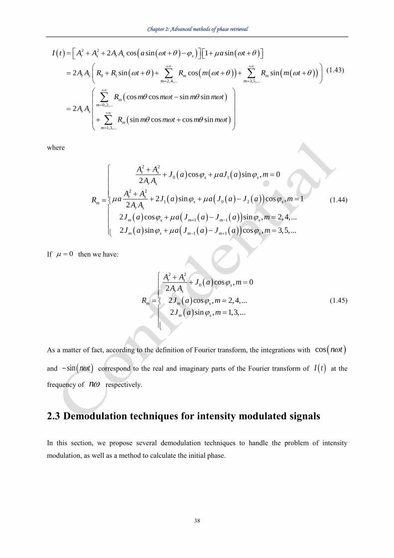
Chapter 2: Advanced methods of phase retrieval
38
( ) ( )( ) ( )
( ) ( )( ) ( )( )
( )
( )
2 2
1
2,4,... 3,5
0
,...
0,2,...
1,3,...
2 cos sin 1 sin
2 sin cos sin
cos sin
2
sin cos cos s
cos i
n
s n
i
r s r
m
s s
r s m
m
r s
m
m
m
m
m
I t A A A A a t a t
A A R t m t R m t
m t m t
A A
R m m t m m t
R R
R m m
+ +
= =
+
=
+
=
= + + + − + +
= + + + + +
−
=
+
+ +
(1.43)
where
( ) ( )
( ) ( ) ( )( )
( ) ( ) ( )( )( ) ( ) ( )( )
2 2
0 1
2 2
1 0 2
1 1
1 1
cos sin2
2 sin cos , 12
2 c
, 0
, 2,4,...
, 3,5,..
n
.
os si
2 sin cos
r ss s
r s
r ss s
r s
m s m m s
m s s
m
m m
m
R
A AJ a aJ a
A A
A Aa J a a J a J a m
A A
J a a J a J ma
J a a J ma J a
+ −
− +
+ =
= + =
+ = −
++
++ + − =
−
(1.44)
If 0 = then we have:
( )
( )
( )
2 2
0 cos2
2 cos
2 sin
.
, 0
, 2,4, ..
, 1,3,...
m m
r ss
r s
s
m s
m
R
A AJ a
A A
J a
mJ a
m
=
= =
++
=
(1.45)
As a matter of fact, according to the definition of Fourier transform, the integrations with ( )cos n t
and ( )sin n t− correspond to the real and imaginary parts of the Fourier transform of ( )I t at the
frequency of n respectively.
2.3 Demodulation techniques for intensity modulated signals
In this section, we propose several demodulation techniques to handle the problem of intensity
modulation, as well as a method to calculate the initial phase.

Chapter 2: Advanced methods of phase retrieval
39
2.3.1 Modified SPM algorithm
We know that in SPM algorithm, the definitions of ( )C t and ( )S t are:
( ) ( )cos 2C t t= , (1.46)
( ) ( )sinS t t= . (1.47)
Then according to the orthogonality of trigonometric functions, we have:
( ) ( )
( ) ( ) ( ) ( )( )( )0
1 1cos 2 2 cos sin
T
r s m s m m s
X I t C t dt
TA A J a a J a J a + −
=
= −+
(1.48)
( ) ( )
( ) ( ) ( )( )
0
2 2
1 0 2cos 2 sin cos2
T
r sr s s s
r s
Y I t S t dt
A ATA A a J a a J a J a
A A
=
+= + + −
(1.49)
If we define the following coefficients:
( )2 2
0
1cos
2r sQ aT A A = + (1.50)
( )1 12 cosr sQ TA A J a= (1.51)
( ) ( )( )2 0 2cosr sQ aTA A J a J a = − (1.52)
( ) ( )3 2 cos 2r s mTA A J aQ = (1.53)
( ) ( ) ( )( )14 1cos 2r s m maTA A J a J aQ + −−= (1.54)
Then we obtain an equation set:
0 1 2sin coss sY Q Q Q = + + (1.55)
3 4cos sins sX Q Q = + (1.56)

Chapter 2: Advanced methods of phase retrieval
40
The solutions of this equation set are:
4 1 0 4
2 4 1 3
cos s
Q Y Q X Q Q
Q Q Q Q
− −=
− (1.57)
3 2 0 3
1 3 2 4
sin s
Q Y Q X Q Q
Q Q Q Q
− −=
− (1.58)
So we can obtain:
( )arg cos sins s si = + (1.59)
From the derivation above, we can see that the and 2 components are used to obtain s . This
is the basic idea of SPM algorithm. When 0 = , it becomes the case described by [74].
However, according to the frequency domain analysis, the components at other harmonics also contain
information of s (see Eq. (1.44)). If we want to use other components to obtain s , it is feasible as
long as the equation set containing cos s and sin s is solvable. For example, if we want to make
use of the and 2 components, we may redefine ( )S t :
( ) ( )sin 3S t t= (1.60)
Then the Y becomes:
( ) ( )
( ) ( ) ( ) ( )( )( )0
3 2 4cos 3 2 sin cos
T
r s s s
Y I t S t dt
TA A J a a J a J a −+
=
=
(1.61)
Also 1Q and 2Q should be redefined as:
( ) ( )1 32 cos 3r sQ TA A J a= (1.62)
( ) ( ) ( )( )2 2 4cos 3r sQ aTA A J a J a = − (1.63)
Now the equation set becomes:
1 2sin coss sY Q Q = + (1.64)

Chapter 2: Advanced methods of phase retrieval
41
3 4cos sins sX Q Q = + (1.65)
The solutions of this equation set are:
4 1
2 4 1 3
cos s
Q Y Q X
Q Q Q Q
−=
− (1.66)
3 2
1 3 2 4
sin s
Q Y Q X
Q Q Q Q
−=
− (1.67)
This way s can be obtained. The advantage of using 3 instead of is that: the term 0Q , which
used to be the only one containing the term ( )2 2
r sA A+ , becomes zero. This is advantageous because
as discussed in the last chapter, when η<1, which is often the case in reality, it is preferred to avoid using
the DC component in I(t) so that there is no need to measure η. Besides, 1Q , 2Q ,
3Q and 4Q all
contain r sA A so that it can be eliminated, which means it is unnecessary to measure rA and sA .
When choosing the components to be used, the low frequency components (like ω, 2ω and 3ω) should
be chosen in priority, since the high frequency components are usually very weak, which will affect the
precision of measurements. Yet the zero-frequency/DC component of signal is not recommended to be
used, because it can be easily affected (by the ambient light, by the gain/exposure of camera/detector,
etc.).
Another thing to be noticed is that the value of θ should also be considered while choosing the
components. For example, if 4
= , then ( )cos 2 0 = , which means
3 4 0Q Q= = , making 0X = .
In this case, we may choose other frequency components, or change the definition of ( )C t from
( ) ( )cos 2C t t= to ( ) ( )sin 2C t t= .
In practice, the values of θ and μ may be difficult to measure. However, it should be noticed that after a
signal I(t) is obtained, all the frequency components below the Nyquist frequency can be extracted. This
means we have an equation set containing θ, μ, sin φs , cos φs (and eventually a, Ar, As), with some
redundance, to be solved. So if we make full use of this signal, it is hopeful that we may manage to
directly solve the values of θ, μ, φs, etc., or to improve the measurement precision since we have the
redundant equations. But this part of work requires more mathematical skills, so it will not be discussed
in this thesis.

Chapter 2: Advanced methods of phase retrieval
42
2.3.2 Determination of the initial phase
When θ is unknown, we can make use of the signal at the frequency of ω to obtain its value. We may
redefine:
( ) ( )cosC t t= (1.68)
( ) ( )sinS t t= (1.69)
Then according to Eq. (1.45) we have:
( ) ( ) 1
0
sin
T
r sX I t C t dt TA A R = = (1.70)
( ) ( ) 1
0
cos
T
r sY I t S t dt TA A R = = (1.71)
As long as ( ) ( ) ( )( )2 2
1 1 0 22 sin cos 02
r ss s
r s
A AR a J a a J a J a
A A
+= + + − , we have:
( )arg Y iX = + (1.72)
This method is also described in [14] for the special case when µ=0.
2.3.3 Modified f-G-LIA algorithm
According to Eq. (1.43)-(1.44), the DC-filtered signal ( )I t can be expressed as:
( ) ( ) ( ) ( )2 2
0 12 cos sin2
r sr s s s
r s
A AI t I t A A J a aJ a
A A
+
++
= −
(1.73)
We know that in f-G-LIA algorithm, the definitions of ( )C t and ( )S t are:
( ) ( )( )cos sinC t a t= (1.74)
( ) ( )( )sin sinS t a t= (1.75)
So X and Y can be calculated: (see Appendix for a detailed derivation)

Chapter 2: Advanced methods of phase retrieval
43
( ) ( )
( )
( ) ( )
0
2
0 0 0
1 1 0 1
2 sin 2 cos 2 cos2
cos si
2
2 cos 2 sin 2 sin2 2 2
n2
T
r s s
r s s
X I t C t dt
TA A J a J a J a
TA A a J a J a J a J a
=
+ −
+ −
=
+
(1.76)
( ) ( )
( ) ( )
0
2 2
0 0 1
1 1
2 sin 2 cos sin cos2 2
2 cos 2 sin cos2 2 2 2
cos sin
T
r s s r s
r s s
Y I t S t dt
TA A J a J a T A A a J a
TA A a J a J a
=
= − +
+ −
+
(1.77)
If we define the following coefficients:①
( ) ( )2 2
0 1cosr sQ T A A a J a = + (1.78)
1 0 02 sin 2 cos2 2
r sQ TA A J a J a
= −
(1.79)
2 1 12 cos 22
cos si sin2 2
n2
r sQ TA A a J a J a
= −
(1.80)
( )2
0 0 03 2 sin 2 cos 22 2
r sQ TA A J a J a J a
+ −
=
(1.81)
( ) ( )14 1 0 12 cos 2s si in 22 2 2 2
cos nr sQ TA A a J a J a J a J a
+ − =
(1.82)
Then we obtain an equation set:
0 1 2sin coss sY Q Q Q = + + (1.83)
3 4cos sins sX Q Q = + (1.84)
The solutions of this equation set are:
① In practice, when the interference is not perfect (0<η<1), the value of η should be considered.
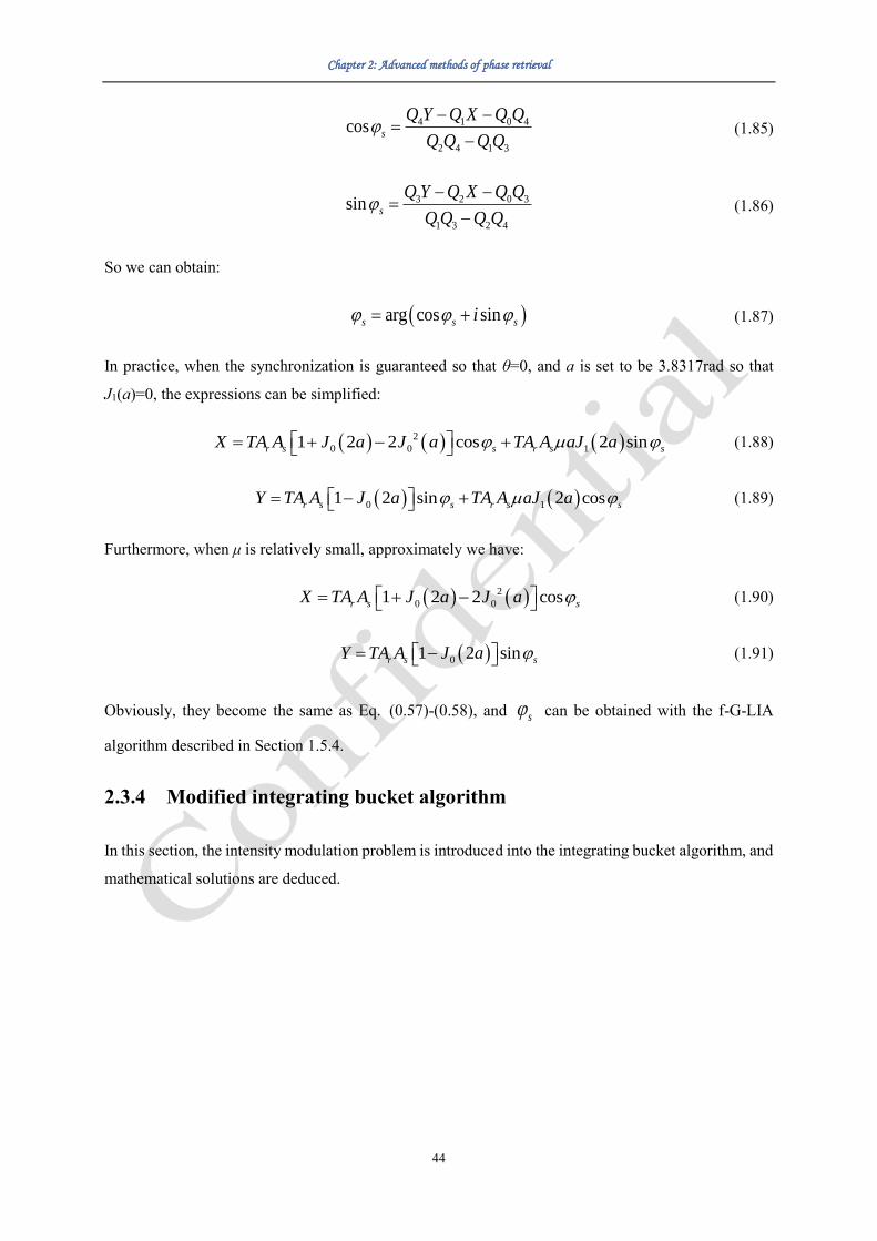
Chapter 2: Advanced methods of phase retrieval
44
4 1 0 4
2 4 1 3
cos s
Q Y Q X Q Q
Q Q Q Q
− −=
− (1.85)
3 2 0 3
1 3 2 4
sin s
Q Y Q X Q Q
Q Q Q Q
− −=
− (1.86)
So we can obtain:
( )arg cos sins s si = + (1.87)
In practice, when the synchronization is guaranteed so that θ=0, and a is set to be 3.8317rad so that
J1(a)=0, the expressions can be simplified:
( ) ( ) ( )2
0 0 11 2 2 cos 2 sinr s s r s sX TA A J a J a TA A aJ a + +−= (1.88)
( ) ( )0 11 2 sin 2 cosr s s r s sY TA A J a TA A aJ a = − + (1.89)
Furthermore, when μ is relatively small, approximately we have:
( ) ( )2
0 01 2 2 cosr s sX TA A J a J a + − = (1.90)
( )01 2 sinr s sY TA A J a = − (1.91)
Obviously, they become the same as Eq. (0.57)-(0.58), and s can be obtained with the f-G-LIA
algorithm described in Section 1.5.4.
2.3.4 Modified integrating bucket algorithm
In this section, the intensity modulation problem is introduced into the integrating bucket algorithm, and
mathematical solutions are deduced.

Chapter 2: Advanced methods of phase retrieval
45
According to the integral properties of trigonometric functions, it can be easily calculated that:
( )f t
1 0 ( )( )cos 2 1n t−
( )( )sin 2 1n t−
( )cos 2n t
( )sin 2n t
( )2
0f t dt
2
0 ( )
( )
1
2 1
n
n
− −
−
( )1
2 1n −
0 ( )1 1
2
n
n
− −
( )2
f t dt
2
0 ( )
( )
1
2 1
n
n
−
−
( )1
2 1n −
0 ( )1 1
2
n
n
− −
( )3
2 f t dt
2
0 ( )
( )
1
2 1
n
n
−
−
( )1
2 1n
−
−
0 ( )1 1
2
n
n
− −
( )2
3
2
f t dt
2
0 ( )
( )
1
2 1
n
n
− −
−
( )1
2 1n
−
−
0 ( )1 1
2
n
n
− −
Table 2-1. Integrals of trigonometric functions over quarter periods.
We define U1, U2, U3, U4 as follows:
( )21
0U I t dt
= (1.92)
( )2
2
U I t dt
= (1.93)
( )3
23U I t dt
= (1.94)
( )2
34
2
U I t dt
= (1.95)
U1, U2, U3, U4 are the values which can be directly measured, as the exposure process of digital camera
can be seen as the integration of light intensity over time. We can deduce that:

Chapter 2: Advanced methods of phase retrieval
46
( )
( )
2
2,4,...
11
2
1,3,...
0
s
s1 1
22
o
i
1 1in s
n
c
m
m
mr s
m
m
m mm
U A A
R m mm m
R R
+
=
++
=
− −
=
− − + +
−
(1.96)
( )
( )
2
0
2,4,...
12
2
1,3,...
1 1
22
1 1sin co
sin
s
m
m
m
mr s
m
m
mm
U
R
A A
R m
R
mm m
+
=
++
=
− −
=
− + +
−
(1.97)
( )
( )
2
2,4,...
1
1
0
3
2
,3,...
1 1
22
1 1s
s
in cos
inm
m
m
mr s
m
m
mm
U
R
A A
R m
R
mm m
+
=
++
=
− −
=
− − + +
−
(1.98)
( )
( )
2
0
2,4,...
14
2
1,3,...
1 1
22
1 1sin co
sin
s
m
m
m
mr s
m
m
mm
U A A
R m mm
R R
m
+
=
++
=
− −
=
− − − + +
−
(1.99)
where the functions Rm (m=0,1,2,…), which contain information of φs, are defined by Eq. (1.44). If we
define three new functions as follows:
( ) 2
1
2,4,...
sin1 1
m
m
m
L mRm
+
=
− −= (1.100)
( )
1
2
2
1,3,...
1sin
m
m
m
L R mm
++
=
− −= (1.101)
3
1,3,...
1cosm
m
L R mm
+
=
= (1.102)
Then we can simplify the expressions for U1, U2, U3, U4:

Chapter 2: Advanced methods of phase retrieval
47
01 1 2 322
r sU A A LR L L
= + +
− (1.103)
02 1 2 322
r sU A A L L LR
= + − +
(1.104)
03 1 2 322
r sU A A LR L L
= − −
− (1.105)
04 1 2 322
r sU A A L L LR
= + + −
(1.106)
In this equation set, since U1, U2, U3 and U4 can be measured in the experiments, we can obtain the
values of R0, L1, L2 and L3 by solving this equation. For example:
1 2 3 4
242 r s
U U U UL
A A
− + + −− = (1.107)
1 2 3 4
142 r s
U U U UL
A A
− + − += (1.108)
Besides, according to the definitions of L1 and L2, we also have:①
( )( )
( )
( ) ( )( )( )
12 2
2
2
1,3,...
1
2
1 1
1,3,...
2 sin 14 8 sin sin
14 sin cos
m
r s
m s
mr s
m
m m s
m
A AL J a m
A A m
J a J a mm
+
+
=
++
− +
=
− + − − = +
− −
+
(1.109)
( )( )
( ) ( )( )( )
2
1
2,4,...
2
1 1
2,4,...
1 14 ssin
si
8 co
1 14 sn in
m
m s
m
m
m m s
m
L J a mm
J a J a mm
+
=
+
+ −
=
− −
=
− −
+ −
(1.110)
In order to simplify these two equations, we may define:
① In practice, when the interference is not perfect (0<η<1), the value of η should be considered.

Chapter 2: Advanced methods of phase retrieval
48
( )2
0
22 sinr s
r s
QA A
A A
− += (1.111)
( )( )
1
2
1
1,3,...
18 sin
m
m
m
Q J a mm
++
=
−= (1.112)
( ) ( )( )( )
1
2
2 1 1
1,3,...
14 sin
m
m m
m
Q J a J a mm
++
− +
=
−= − (1.113)
( )( ) 2
3
2,4,...
si11
n8
m
m
m
Q J a mm
+
=
− −= (1.114)
( ) ( )( )( ) 2
4 1 1
2,4,...
1 1in4 s
m
m m
m
Q J a J a mm
+
+ −
=
− −= − (1.115)
21 4P L= − (1.116)
12 4P L= (1.117)
So Eq. (1.109)-(1.110) can be expressed as:
1 0 1 2sin coss sP Q Q Q = + + (1.118)
2 3 4cos sins sP Q Q = + (1.119)
These two equations can be seen as an equation set of sinφs and cosφs since the values of P1, P2, Q0,
Q1, Q2, Q3, and Q4 can all be obtained. This equation set can be easily solved:
4 1 1 2 0 4
2 4 1 3
cos s
Q P Q P Q Q
Q Q Q Q
− −=
− (1.120)
3 1 2 2 0 3
1 3 2 4
sin s
Q P Q P Q Q
Q Q Q Q
− −=
− (1.121)
Then the signal phase can be obtained:
( )arg cos sins s si = + (1.122)

Chapter 2: Advanced methods of phase retrieval
49
If μ=0 which is the case described by the reference [81], then, Q0 = Q2 = Q4 = 0 so we have:
2
3
cos s
P
Q = (1.123)
1
1
sin s
P
Q = (1.124)
For the integrating bucket method, it is important to choose the right value of θ. Obviously, if 0 =
then L1 = L2 = 0, making it impossible to retrieve the phase information s . In this case, we may
redefine P1 and P2 to retrieve the values of R0 and L3 instead. However, R0 often contains DC noise,
which may drastically reduce the measurement precision of s . So it is preferred to choose a good
value of θ in order to make the integrating bucket method works. Besides, the values of a and µ may
also have an influence on the final results, since they are widely present in the coefficients. When μ=0
, in order to minimize the effect of Gaussian additive noise (to have a zero mean phase error for any s ,
and to get the minimum mean square phase error), we should set 2.45a rad= and 0.98rad =
[26,81]. Recently, the values 2.08a rad= and 4 2
n
= + (n is an integer) have also been used
in a simplified algorithm [87]. This way, the phase of signal may be calculated correctly without even
knowing which image is the first one in the sequence of images.
2.4 Conclusion
In this chapter, the initial phase problem in phase modulating interferometer is mentioned and
mathematically described. This problem is not a real issue when using linear/sawtooth modulation (see
Section 2.1.1); when using a sinusoidal phase modulation, the value of the initial phase may be
calculated from the interference signal (see Section 2.3.2). When this problem cannot be eliminated, its
influence on the phase detection is discussed in Section 2.1.
The intensity modulation problem is described. To solve this issue, the affected interference signal is
analyzed in the frequency domain (see Section 2.2.1), and a modified SPM algorithm is proposed based
on it (see Section 2.3.1). Besides, we also make modifications to the f-G-LIA algorithm (see Section
2.3.3) and the integrating bucket algorithm (see Section 2.3.4) to get rid of the influence of this problem.
By solving these two practical problems, we have now better tools to apply continuous phase modulation
techniques in simple and cost-effective measuring systems, as will be shown in Chapter 3, Chapter 4
and Chapter 5.

Chapter 3: Application of SPM in DH/DHI
51
Chapter 3 Application of SPM in Digital
Holography and Holographic Interferometry
In this chapter, we detail how the G-LIA algorithm can be used in a simple and lens-less interferometric
setup to perform low-cost yet efficient 2D phase measurement, and focus on the performance of G-LIA
algorithm in this system. We first describe the optical system which can also be regarded as a phase-
shifting digital holographic microscope without optical magnification. Digital holography (DH) and
Digital Holographic Interferometry (DHI) capability is demonstrated.
3.1 Experimental method and data processing
The setup we built is a simple and compact one, adapted from a traditional Michelson interferometer.
As shown in the following figure, we replaced one mirror of classical Michelson interferometer by a
scattering sample, the other mirror by a piezo-actuated mirror, and the point detector by a CMOS camera
(without objective lens). It can be seen as a co-axis① digital holography setup.
① Co-axis setups differs from the off-axis ones because the “reference light” reflected by the mirror and the “signal light”
scattered by the sample both hit the CMOS camera from nearly the same direction.

Chapter 3: Application of SPM in DH/DHI
52
Figure 3-1 Co-axis digital holography using sinusoidal phase modulation.
We restricted our study to sinusoidal phase modulation, the most convenient one in practice. We note
that for cheap phase-shifting devices like piezo-actuated mirrors, a sinusoidal modulation function is the
most practical choice. In our case the piezo hysteresis doesn't need to be considered given the short
modulation range, although it could also be included in the modulation function used to extract the phase
information.
By applying sinusoidal phase modulation, (f)-G-LIA algorithm can be compared with SPM algorithm
in the case of digital holography and digital holographic interferometry. Since when 2.4048a rad= ,
f-G-LIA and G-LIA algorithms are the same, for simplicity, SPM and G-LIA algorithms at
2.4048a rad= are compared experimentally.
The sinusoidal phase modulation was achieved by controlling the piezo-actuated mirror with a
waveform generator. We used a red laser emitting at 640nm = (DL640-070-SO, diode laser made
by CrystaLaser, 70mW). For this wavelength, the condition of 2.4048a rad= corresponds to a mirror
oscillation amplitude of about 122nm . This amplitude is adjusted by using a strain gauge sensor
attached to the piezoelectric actuator to measure its deformation and to obtain the mirror displacement.
In fact, with this experimental method, the actual amplitude of phase modulation is estimated to be
2.40 0.05a rad .
Usually at least 5 frames should be taken for each period of modulation to ensure a reasonable sampling
rate. In this experiment, we took 10 frames for each period of modulation. Hence, the maximum
modulation frequency is fixed by the frame rate of the camera given in FPS (frames per second), e.g.
the maximum modulation frequency equals to 1 Hz when recording a video at 10 FPS. For this reason,
high-speed cameras are needed when the measurement has to be done in a short time. However,
depending on the needs, low-speed and cheap cameras can also be used.

Chapter 3: Application of SPM in DH/DHI
53
The beam of the red laser (DL640-070-SO, diode laser made by CrystaLaser, 640nm, 70mW) with an
attenuated power of about 1.4mW was expended up to a diameter of about 1cm to achieve a relatively
homogeneous illumination of the CMOS sensor. Then each image taken by this lens-less CMOS camera
(8-bit, variable frame rate) is an interference pattern between the reference plane wave reflected by the
mirror and the signal light scattered by the sample. The effective numerical aperture depends on the size
of CMOS matrix and the distance from the CMOS to the sample. Usually this distance is several
centimeters, so that in our setup, an effective numerical aperture of NAeff≈0.04 (This value may differ
when the size of CMOS or the distance between sample and camera changes) is obtained. The method
we used to determine NAeff is shown by the figure below.
Figure 3-2 Determination of an effective numerical aperture relative to the sample centre. Ideally, the
sample should be small compared to the CMOS matrix to keep a homogeneous spatial resolution across
the sample. Beside pixel size, a high effective numerical aperture is required to achieve a high-resolution
imaging.
From the video recorded during the reference mirror oscillation, the phase and amplitude of the scattered
signal is obtained on each pixel of the camera using both the G-LIA algorithm and the SPM algorithm
respectively (see Section 1.5) performed in the MATLAB environment. We note that the amplitude of
the signal which can also be obtained without interferometry, is less important than the phase, in the
sense that the sample image is still perceptible from the phase information only, i.e. if we consider a
constant signal amplitude on each camera pixel.
Once the complex light field on the CMOS plane is obtained, the complex light field on the sample
plane can be reconstructed using the angular spectrum method [88,89]: the angular spectrum of plane
waves was determined by 2D Fourier transform, then the plane waves were numerically retro-
propagated from the detector to the sample plane where the best focus is obtained (see Appendix).

Chapter 3: Application of SPM in DH/DHI
54
For a proper operation, the recorded signal I(t) should be synchronized with C(t) and S(t). Otherwise a
non-zero initial phase θ can appear in the signal:
( ) ( )( )2 2 2 cos sinr s r s sI t A A A A a t = + + + − (1.125)
Synchronization can be done by triggering the camera recording together with the start of sinusoidal
phase modulation. Alternately, the initial phase θ can be calculated pixel by pixel with the recorded
video using the harmonic component of ω in the signal I(t) (see Section 2.3.2). Experimentally, since
the mirror movement corresponds to a rigid body oscillation, the average value of calculated initial
phases (or the calculated initial phase using the average intensity signal over many pixels) can be
considered to be the real initial phase for each pixel to reduce the error. Once we have the value of the
initial phase, we can adjust C(t) and S(t) accordingly — which is more practical than adjusting I(t) —
and carry out the algorithms discussed in Section 1.5.
3.2 Digital holography (DH)
A USAF 1951 resolution test target was observed to test the spatial resolution of our system. A camera
with a pixel size of 5.2µm5.2µm was used. The frame rate was set to 10 FPS, and the modulation
frequency was set to 1 Hz. By using only 10 images (1 period of modulation), high-quality results can
be obtained. As shown in the Figure 3-3 hereafter, although the phase image is a little noisy, our system
which is operated in a standard environment can be used to carry out the lens-less imaging, and the
profile of the surface can be measured.
Another experiment is done to compare the performance of G-LIA and SPM algorithms. The results are
shown in Figure 3-4

Chapter 3: Application of SPM in DH/DHI
55
Figure 3-3 Test with USAF 1951 resolution test target. The pixel size of camera is 5.2µm5.2µm . (a)
The positive 1951 USAF test target “R1DS1P” is from the company ThorLabs [90]. (b) Phase image
obtained by G-LIA algorithm. (c) Profiles of the sixth element of the second group, which is highlighted
by the green rectangles in (a)(b). (d) 3D profile image of the sixth element of the second group.

Chapter 3: Application of SPM in DH/DHI
56
Figure 3-4 Holographic images obtained with G-LIA and SPM algorithms. Left column: light intensity
images of the resolution test target. Middle column: zoomed-in light intensity images showing the first
three elements of the fifth group of the resolution test target. Right column: phase images (without 2D
unwrapping) of the resolution test target.
According to Figure 3-4, visually G-LIA and SPM algorithms give almost the same results. The smallest
distinguishable pattern is the first element of the fifth group for both of them (as shown in the middle
column of Figure 3-4), which means the spatial resolution of this setup can reach 32 LP/mm (LP: line
pair), or 15.6μm, for both G-LIA and SPM algorithms. Although this resolution is not comparable to
the current high-resolution [91] or super-resolution [92,93] digital holography microscopes [94], which
can usually reach a spatial resolution around 1μm, it is reasonable (as detailed later in this section) for
the proposed lens-less setup, which is sufficient to test the performance of the phase retrieval algorithms.
In order to show this resolution clearly and to better compare G-LIA and SPM algorithms, 1D
normalized profiles of the first element of the fifth group are represented in the following figure. The
pattern representing resolution of 32 LP/mm is clearly distinguished, and the results given by G-LIA
and SPM algorithms are nearly identical, except that the peak-to-peak values for the G-LIA algorithm
is slightly bigger (higher contrast).

Chapter 3: Application of SPM in DH/DHI
57
Figure 3-5 Normalized profiles of the light intensity images using SPM and G-LIA algorithms. Two
profiles (a) and (b) were taken on the first element of the fifth group of the resolution test target.
If all the wavevectors of the light scattered by the sample are collected, then the resolution is mostly
limited by the spatial sampling given by the distance between camera pixels (5.2µm in both directions),
since a lens-less system was used and there was no optical magnification. It can be easily calculated that
32 LP/mm means 6 pixels/LP, which is close to the limit of 2 pixels/LP given by the Nyquist–Shannon
sampling theorem. It is hard to actually reach this theoretical limit for several reasons. First of all, the

Chapter 3: Application of SPM in DH/DHI
58
wavevectors are not totally collected by the system with the effective numerical aperture NAeff≈0.04
(corresponding to about 10µm resolution according to the Rayleigh criterion). Also, the digital data
acquisition itself is affected by experimental noises, as well as slight measurement error on the value of
a. Besides, theoretically, the angular spectrum method that we used for light field reconstruction is based
on Fourier transform and is affected by the finite size of the sensor. Therefore, the obtained 6 pixels/LP
resolution can be reasonably accounted for.
Another thing that we can observe from Figure 3-5 is that the background level of the phase image is
not perfectly flat. However, the observed phase variations are within one wavelength which is
reasonable, since the sample is not perfectly flat. We note that the substrate positioning also induces
residual tilts with respect to the direction of incident beam which is not a perfect plane wave either.
We also made a test on the influence of spatial phase noise on the final spatial resolution. The results
are shown in the figure below.
Figure 3-6 Zoomed-in light intensity images showing the first three elements of the fifth group of the
resolution test target with 2D white Gaussian noises added to the obtained phase image. (a) Without
noise. (b) Power of noise: -20dBW. (c) Power of noise: -9dBW. (d) Power of noise: -5dBW.
From Figure 3-7 we can see that as the power of noise goes bigger, the pattern becomes more blurred.
When the power of noise reaches -5dBW, the first element of the fifth group becomes indistinguishable.
Yet we noticed that with a power of noise smaller than -9dBW, the first element of the fifth group can
be distinguished, which means the spatial resolution will not be affected when the phase noise is small.
We also considered the case when several pixels cannot provide phase information, e.g. when the pixels
are broken. For these pixels, we set the phase as zero. A test is done with different numbers of such
pixels. The results are shown in the following figure.

Chapter 3: Application of SPM in DH/DHI
59
Figure 3-8 Zoomed-in light intensity images showing the first three elements of the fifth group of the
resolution test target with the phase of several pixels in the middle of this zone set to zero. The size of
the selected zone is 100×100 pixels. (a) 1×1 pixel. (b) 10×10 pixels. (c) 30×30 pixels. (d) 100×100
pixels.
As shown in Figure 3-9, if the defection is small (from 1 pixel to 10×10 pixels), then it will not have an
obvious influence on the spatial resolution; when it reaches 30×30 pixels, a ring ripple becomes obvious,
which blurred the pattern to some extent. Finally, when all the phase information in this zone is lost, as
shown in Figure 3-10 (d), the first element of the fifth group can hardly be distinguished; yet some parts
of the pattern can be observed, since the phase information at the neighboring zone is good. In fact, it is
an intrinsic property of holography: we do not need the whole hologram to reconstruct the image of
object. [31]
3.3 Digital holographic interferometry (DHI)
For digital holographic interferometry (DHI), the same methods were used to obtain the light field on
the CMOS plane and then the same numerical reconstruction was done to get the light field on the
sample surface. According to the theory of holographic interferometry [31], by subtracting the sample
light field after a small deformation/displacement ( ( )22 2 exp sE A i= ) from the one before (
( )11 1 exp sE A i= ), fringes can be observed in the image of 2 1E E− , or in the image of
( )2 1
cos s s − for a better contrast.①
① Through angular spectrum method (see Appendix), the complex field difference can be calculated at different positions,
and the corresponding fringe images can be obtained.

Chapter 3: Application of SPM in DH/DHI
60
Considering the sensitivity vector① [31] of our system which is almost perpendicular to the sample
surface, these fringes mainly account for the out-of-plane displacement field. In the same way, when the
sample is purely rotated out of plane, the reconstructed plane with the best fringe visibility coincide with
the sample surface [31]. However, in practice, a minor in-plane displacement may slightly shift these
two planes away from each other.
In these experiments, the measuring system remains the same (see Figure 3-1), and videos are recorded
at different deformation/displacement states. A camera with a pixel size of 3.63µm3.63µm was used.
Its frame rate was set to 120 FPS, and the phase modulation frequency was set to 10 Hz. By using only
12 images (1 period) for each measurement, good quality results are obtained.
Figure 3-11 The one euro cent coin sample. (a) Photo of the coin. (b) Amplitude of the scattered light field at the
plane of sample surface calculated by G-LIA algorithm. (c) Phase of the scattered light field at the plane of sample
surface calculated by G-LIA algorithm.
A coin of one euro cent was used as scattering sample (see Figure 3-11). Unlike Figure 3-4, the phase
image does not exhibit distinctive patterns. It shows that the coin has a complex and optically rough
surface, inducing speckle-like scattering. A small zone of interest was selected by covering the outer
part of the zone with a black tape. The coin was fixed on a rotation stage allowing for a nearly pure out-
of-plane rotation around the vertical axis (minimum scale: 0.04°). The reconstructed planes giving the
best fringe visibility were nearly coinciding with the sample surface. (In Figure 3-11, the images were
obtained on a plane which is 70mm away from the plane of the CMOS, while in Figure 3-12 and Figure
3-13 this distance was 68mm.)
① For a certain point on the sample, the sensitivity vector is the difference between the unit vectors representing the
directions of illumination and viewing of that point.

Chapter 3: Application of SPM in DH/DHI
61
Figure 3-12 and Figure 3-13 show the results obtained for rotations of about 0.02° and 0.04°, obtained
by G-LIA and SPM algorithms by using the two complex field images E1 and E2.
Figure 3-12 Image of 2 1E E− obtained by using G-LIA and SPM algorithms for out-of-plane
rotations of about 0.02° and 0.04°.

Chapter 3: Application of SPM in DH/DHI
62
Figure 3-13 Image of ( )2 1
cos s s − obtained by using G-LIA and SPM algorithms for out-of-plane
rotations of about 0.02° and 0.04°.
We can see from Figure 3-12 and Figure 3-13 that the visibility of the fringes is very good. The covered
zone is much noisier than the zone of interest because the black tape could barely scatter light. The
fringe visibility is better in Figure 3-13 where only the phase information is used, but it looks naturally
noisier than Figure 3-12 near the edges where the signal is low (the phase always gives a value in its
definition interval of 2 while the amplitudes goes to zero when the signal is weak). Given the
relatively high frequency nature of this noise, these fast fluctuations can be suppressed by a low-pass
spatial filter without affecting the fringes describing the rotation (see Figure 3-15).

Chapter 3: Application of SPM in DH/DHI
63
As shown in Figure 3-12 and Figure 3-13, the fringes orientation is almost vertical, i.e. parallel to the
rotation axis. The number of fringes k we obtain can be compared with the theoretical expectation for
0.02°:
2 3.63 / 1280 sin 0.02
5.07640
m pixel pixelk
nm
= (1.126)
This k value is in agreement with the Figure 3-13 showing about 5 fringes. Likewise, for a rotation of
about 0.04°, the theoretical fringe number is 10.14, while we can observe around 10.5 fringes in Figure
3-13. A sensitivity better than 0.004° (corresponding to one single fringe in the whole image) can hence
reasonably be obtained, for example 0.0004°, if a variation of one tenth of a fringe is detected with
proper algorithms of fringe analysis.
From Figure 3-12 and Figure 3-13, no difference between the results given by G-LIA and SPM
algorithms can be seen visually. In order to make a clearer comparison, profiles of the fringes presented
in the left column of Figure 3-13 are shown in Figure 3-14; then these images of fringes went through
a 2D low-pass filter so that the noise can be suppressed, and the profiles at the same position are shown
in Figure 3-15.

Chapter 3: Application of SPM in DH/DHI
64
Figure 3-14 Profiles of the fringes in the unfiltered image of ( )2 1
cos s s − obtained by G-LIA and
SPM algorithms respectively for an out-of-plane rotation of about 0.02°.
Figure 3-15 Profiles of the fringes in the filtered image of ( )2 1
cos s s − obtained by G-LIA and SPM
algorithms respectively for an out-of-plane rotation of about 0.02°.
Chapter 3: Application of SPM in DH/DHI
65
Further analysis of Figure 3-14 shows that although the exact values obtained by G-LIA and SPM
algorithms differ, their noise levels are nearly the same as expected from the simulations performed
before. As shown in Figure 3-15, the high frequency noise can be efficiently suppressed using a 2D
low-pass filter, and the same smooth profile was obtained by both G-LIA and SPM algorithms.
However, when a simple low-pass filter is directly applied to the image of ( )2 1
cos s s − , error will
occur on the results of φS2 - φS1. As shown in Figure 3-15, the value of ( )2 1
cos s s − never reaches
1, which is not reasonable and will affect the precision of fringe count. To solve this problem, we may
use the following phase filtering method:
1. Calculate the images ( )2 1
cos s s − and ( )2 1
sin s s − from the image of 2 1s s − ;
2. The images of ( )2 1
cos s s − and ( )2 1
sin s s − are filtered respectively;
3. The new image of phase can be obtained: ( ) ( )2 1 2 1 2 1
coarg s sins s s s s si =− − −
+ ;
4. If necessary, repeat step 1 to 3 several times (iterative method).
In Step 2, different ways of filtering are usable: we may keep using the simple low-pass filter, or we can
use the conventional 2D convolution method [95,96]. The results are shown in Figure 3-16 and Figure
3-17 respectively.

Chapter 3: Application of SPM in DH/DHI
66
Figure 3-16 Profiles of the fringes in the image of filtered ( )2 1
cos s s − obtained by G-LIA and SPM
algorithms respectively for an out-of-plane rotation of about 0.02°. Phase filtering method with low-
pass filtering was used, and the number of iterations is 1.
Figure 3-17 Profiles of the fringes in the image of filtered ( )2 1
cos s s − obtained by G-LIA and SPM
algorithms respectively for an out-of-plane rotation of about 0.02°. Phase filtering method with 2D
convolution filtering was used, and the number of iterations is 200. The kernel used is Gaussian blur
11×11 with a standard deviation of 0.8.
From Figure 3-16 and Figure 3-17, we can see the problem of Figure 3-15 can be solved by using this
phase filtering method, and the results given by G-LIA and SPM algorithms are still almost the same.
Chapter 3: Application of SPM in DH/DHI
67
In Figure 3-16 and Figure 3-17, the fringe qualities are nearly the same, however the fringe counts are
slightly different, which is caused by the different filtering methods in Step 2 as well as the different
numbers of iterations. It should be noticed that for the simple fringe image discussed here, low-pass
Fourier filtering (number of iterations: 1) is much more effective than the convolution filtering (number
of iterations: 200). However, when the fringe image is complicated and contains very fine fringes (see
Chapter 5), the convolution filtering is more suitable.
3.4 Conclusion
From the discussions above, we can see that by using sinusoidal phase modulation with G-LIA algorithm
or SPM algorithm, our lens-less digital holography imaging system can reach a spatial resolution of
32 LP/mm which is reasonable given the effective numerical aperture and the pixel size of our system.
This method has the potential to be applied in the well-established digital holographic microscopes
[97,98] with high NA objective lenses, in order to reach a much higher spatial resolution. Besides,
holographic interferometric fringes of out-of-plane rotation could be observed clearly, with highly
visible and predictable fringes given by rotation angles as small as 0.004°. Since DHI can be applied not
only in the displacement measurement but also in a lot of circumstances [99,100,101] where the change
of wavefront of signal needs to be measured, the discussed phase retrieval algorithms may also have a
wide range of applications.
It was proved that for each measurement, data from only one period of sinusoidal modulation was
enough to perform a correct analysis, with sampling rate of about 10 images/period. Compared to the
SPM algorithm, G-LIA algorithm showed similar capacity of retrieving phase information in digital
holography (or holographic interferometry) while having the potential of using a variety of other
modulation functions. This advantage may be important for any situation where another type of
modulation function becomes the most practical choice in the future. Besides, it can be expected that
when the frequency spectrum of noise is known, a certain type of modulation function may be chosen
accordingly in order to improve the anti-noise ability.
As for displacement field measurement, a limitation of the proposed configuration for DHI is that the
sensitivity vector is essentially along the vertical direction, making it mainly sensitive to out-of-plane
displacement. Yet in the next chapter, we will mainly focus on the in-plane displacement field
measurement using continuous phase modulation techniques.


Chapter 4: 2D-ESPI with double phase modulations
69
Chapter 4 2D-ESPI with double phase modulations
Electronic/Digital speckle pattern interferometry (ESPI/DSPI) is a well-established non-contact
detection method. It has been widely used to carry out precise displacement field measurements.
However, the simultaneous 2D or 3D displacement field measurements using ESPI with phase shifting
usually involve complicated and slow equipment. To solve these issues, we proposed a modified ESPI
system based on a single laser and the use of an original modulation technique: by applying two phase
modulations at different frequencies in two different illumination arms, the whole 2D displacement field
is extracted from short video sequences recorded at each deformation state. In-plane normal and shear
strains are then obtained with good quality. This system can also be further developed to measure 3D
deformation, and it has the potential to carry out faster measurements with a high-speed camera.
4.1 Introduction
Before the introduction of digital cameras and computers, the speckle phenomenon was already used to
measure displacement fields; two major types of speckle technique were known as “speckle pattern
photography” and “speckle pattern correlation interferometry” [31]. The first technique, speckle pattern
photography, which is based on the analysis of the speckle displacement, requires a single coherent
beam, and it can be used to measure relatively large in-plane deformation. The second approach, speckle
pattern photography, which is interferometric, requires at least two coherent laser beams. Thanks to the
phase information, it can measure minute in-plane deformations or out-of-plane deformations depending
on the impinging light direction.
As mentioned in the general introduction, with the introduction of digital instruments, the two
approaches have evolved to Digital Speckle Photography (DSP) and Electronic/Digital Speckle Pattern
Interferometry (ESPI/DSPI) respectively.
In-plane deformations can be easily measured by a simple ESPI measuring system [31]. In such system,
the temporal phase-shifting technique is often applied for phase retrieval to improve the performance
[35]. However, in a standard, two-beam, configuration, only one displacement component is measured.
This direction is fixed by the orientation of the laser beams.

Chapter 4: 2D-ESPI with double phase modulations
70
Figure 4-1 Typical phase-shifting ESPI setup for 1D in-plane displacement measurement.
In order to measure the 2D in-plane displacement field (or the whole 3D displacement field), several
solutions have been proposed. The most direct one is to use DSP for the 2D in-plane measurement (or
to combine DSP with out-of-plane ESPI for the 3D measurement) [102]. Nevertheless, the sensitivity of
DSP is not as good as ESPI. A natural solution is then to combine ESPI measuring systems [103,53].
More recently, in-plane ESPI measurement systems were notably combined with out-of-plane ESPI to
perform 3D analysis using optical switches, with a limited time resolution though due to the iterative
process requirement [104,54,55]. To solve the time issue, spatial phase-shifting technique can be
applied: for example, using three lasers producing three spatial frequency carriers [104]. The latter
approach however inevitably makes the whole system substantially more complex and expensive.
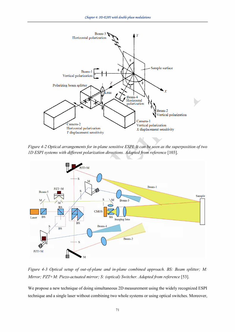
Chapter 4: 2D-ESPI with double phase modulations
71
Figure 4-2 Optical arrangements for in-plane sensitive ESPI. It can be seen as the superposition of two
1D ESPI systems with different polarization directions. Adapted from reference [103].
Figure 4-3 Optical setup of out-of-plane and in-plane combined approach. BS: Beam splitter; M:
Mirror; PZT+M: Piezo-actuated mirror; S: (optical) Switcher. Adapted from reference [53].
We propose a new technique of doing simultaneous 2D measurement using the widely recognized ESPI
technique and a single laser without combining two whole systems or using optical switches. Moreover,

Chapter 4: 2D-ESPI with double phase modulations
72
this technique also has the potential to handle 3D measurement at relatively high speed with minor
modifications. Instead of using the traditional phase-shifting technique, we simultaneously apply two
continuous phase modulations and a short video is taken (e.g. 1 second or much less depending on
camera speed) at each deformation state. During data processing, by selecting the right frequencies, the
displacements along two different directions can be extracted separately.
4.2 Experimental Method and Data Processing
4.2.1 Optical arrangement
The proposed optical arrangement is shown in the figure below. There are three coherent laser beams
originating from a single laser: Beam-1, Beam-2 and Beam-3. The phases of Beam-1 and Beam-2 can
be modulated by the corresponding piezo-actuated mirrors.
Figure 4-4 Setup for ESPI measurement. (a) Top view; (b) 3D view. The camera is above the sample to
take photos of its surface. The height and focus of camera can be adjusted to get different magnifications.
The optics plane is a little above the sample plane so that the surface can be illuminated by laser beams.

Chapter 4: 2D-ESPI with double phase modulations
73
Laser: CNI MSL-532 (diode-pumped solid-state laser, 532nm, 20mW). Camera: Flea®3 FL3-U3-
13S2M-CS 1/3" Monochrome USB 3.0 Camera. CL: Concave lens. CM: Concave mirror. BS: Beam
splitter. PZT+M: Piezo-actuated mirror.
4.2.2 Principle of measurement
If Beam-1 is blocked, then it becomes a typical phase-shifting ESPI system that measures deformation
along X-axis. Likewise, if Beam-2 is blocked, then it is sensitive to the deformation along Y-axis. When
none of them is blocked and two temporal phase modulation functions, F1(t) and F2(t), are applied to
Beam-1 and Beam-2 respectively, the scalar light field of the subjective speckles E(x,y) can be expressed
as:
( ) ( ) ( ) ( ) ( ) ( ) ( ) ( ) ( )1 1 2 2 32 , 2 , 2 ,
1 2 3, , , ,c c ci f t x y F t i f t x y F t i f t x yE x y A x y e A x y e A x y e
+ + + + + = + + (2.1)
Am(x,y) and θm(x,y) are the amplitude and the initial phase of Beam-m (m=1,2,3) at point (x,y)
respectively, and fc is the optical frequency of laser.
On the sample surface, the light intensity I(x,y) can be expressed as:
( ) ( )
( ) ( ) ( ) ( ) ( ) ( ) ( ) ( ) ( )
( ) ( ) ( ) ( ) ( ) ( ) ( ) ( ) ( ) ( )
2
2 2 2
1 2 3 1 2 1 1 2 2
1 3 1 1 3 2 3 2 2 3
, ,
, , , 2 , , cos , + , -
+2 , , cos , + , +2 , , cos , + ,
I x y E x y
A x y A x y A x y A x y A x y x y F t x y F t
A x y A x y x y F t x y A x y A x y x y F t x y
=
= + + + −
− −
(2.2)
After a small displacement u(x,y), the light intensity turns into:
( ) ( )
( ) ( ) ( ) ( ) ( ) ( ) ( ) ( ) ( )
( ) ( ) ( ) ( ) ( ) ( ) ( ) ( ) ( ) ( )
2
2 2 2
1 2 3 1 2 1 1 2 2
31 3 1 1 2 3 32 2
, ,
, , , 2 , , cos , + , -
+2 , , cos , + , +2 , , cos , + ,
I x y E x y
A x y A x y A x y A x y A x y x y F t x y F t
A x y A x y x y F t x y A x y A x y x y F t x y
=
= + + + −
− −
(2.3)
With
( ) ( ) ( ) ( )1 1 1
2, , ,x y x y x y
= + − sn n u (2.4)
( ) ( ) ( ) ( )2 2 2
2, , ,sx y x y x y
= + −n n u (2.5)
( ) ( ) ( ) ( )3 3 3
2, , ,sx y x y x y
= + −n n u (2.6)

Chapter 4: 2D-ESPI with double phase modulations
74
where λ is the wavelength of laser, nm is the unit vector along illumination direction of Beam-m
(m=1,2,3), ns is the unit vector along viewing direction. nm and ns can be roughly considered to be the
same for every point (x,y) on the sample surface.
If we choose the following linear (or sawtooth) modulation functions:
( )1 12F t f t= (2.7)
( )2 22F t f t= (2.8)
then we have:
( ) ( ) ( ) ( ) ( ) ( ) ( ) ( )
( ) ( ) ( ) ( ) ( ) ( ) ( ) ( )
2 2 2
1 2 3 1 2 1 1 2 2
1 3 1 1 3 2 3 2 2 3
, , , , 2 , , cos , +2 , -2
+2 , , cos , +2 , +2 , , cos , +2 ,
I x y A x y A x y A x y A x y A x y x y f t x y f t
A x y A x y x y f t x y A x y A x y x y f t x y
= + + + −
− −
.
(2.9)
Obviously, when f1, f2 and |f1-f2| are not equal to each other, with a lock-in detection at f1, θ1(x,y)-θ3(x,y)
can be extracted; with a lock-in detection at f2, θ2(x,y)-θ3(x,y) can be extracted [28]. The same procedure
can be carried out to obtain θ1’(x,y)-θ3’(x,y) and θ2’(x,y)-θ3’(x,y). If we set:
( ) ( ) ( ) ( ) ( )1 1 3 1 3, , , , ,C x y x y x y x y x y = − − − (2.10)
( ) ( ) ( ) ( ) ( )2 2 3 2 3, , , , ,C x y x y x y x y x y = − − − (2.11)
then according to Eq. (2.4)-(2.6), we have:
( ) ( ) ( )1
2, ,C x y x y
= −1 3n n u (2.12)
( ) ( ) ( )2
2, ,C x y x y
= −2 3n n u (2.13)
The z components of n1, n2 and n3 are almost equal, so they will cancel each other out in Eq. (2.12)-
(2.13). Concerning the x and y components of n1, n2 and n3, we can see from Fig. 1 that n1-n3 is parallel
to the Y-axis, and n2-n3 is parallel to the X-axis. So C1(x,y) and C2(x,y) can be expressed as:
( ) ( )1 , ,y yC x g uy x= (2.14)
( ) ( )2 , ,xC x y g u x y= (2.15)

Chapter 4: 2D-ESPI with double phase modulations
75
where g is a measurable constant, ux(x,y) and uy(x,y) are the x and y components of u(x,y) respectively.
This means the 2D in-plane displacement field can be measured. The whole procedure is shown by the
flowchart hereafter.
Figure 4-5 Flowchart of the 2D displacement measurement.
It should be noticed that when piezoelectric actuators are driven to make sawtooth displacements, the
precision cannot be guaranteed, especially at high frequency, where the fly-back time of the mirror
cannot be neglected. The nonlinearity and noise generated by the sudden return becomes unacceptable
when high speed measurement is required. This issue can be addressed with sinusoidal phase
modulations such as:
( )1 1sin 2F t a f t= (2.16)
( )2 2sin 2F t a f t= (2.17)
where a is the amplitude of phase modulation. It should be noticed that f1 and f2 are not randomly chosen.
It is favorable to choose coprime integers①, as will be detailed later. Now we have:
( ) ( ) ( ) ( )
( ) ( ) ( ) ( )
( ) ( ) ( ) ( )
( ) ( ) ( ) ( )
2 2 2
1 2 3
1 2 1 2 1 2
1 3 1 3 1
2 3 2 3 2
, , , ,
2 , , cos , , sin 2 sin 2
+2 , , cos , , sin 2
+2 , , cos , , sin 2
I x y A x y A x y A x y
A x y A x y x y x y a f t a f t
A x y A x y x y x y a f t
A x y A x y x y x y a f t
= + +
+ − + −
− +
− +
(2.18)
① Which means, as a reminder, that the only positive integer that divides both of them is 1.

Chapter 4: 2D-ESPI with double phase modulations
76
As we can see, the situation now seems more complex. In Eq. (2.18), according to the Jacobi–Anger
expansion, in the frequency domain, the third term (representing the interference between Beam-1 and
Beam-3) will be distributed at the integer multiples of f1, and the fourth term (representing the
interference between Beam-2 and Beam-3) will be distributed at the integer multiples of f2. If we set
a=2.4048rad so that J0(a)=0 (J0 is the 0th Bessel function of the first kind), then both of them will not
contain any signal at 0Hz. So in the frequency domain, they will not overlap with each other until the
least common multiple of f1 and f2, which is 63Hz in our case (f1=9Hz, f2=7Hz, 9 and 7 are coprime
integers). This means these two terms can be efficiently separated.
The second term in Eq. (2.18) represents the interference between Beam-1 and Beam-2. It may be
eliminated by playing with the polarization (e.g. linear polarization of 0° for Beam-1, 90° for Beam-2,
and 45° for Beam-3) or the temporal coherence (e.g. optical path length: Beam-1<Beam-2<Beam-3);
but these solutions would surely increase the difficulty of adjusting the measuring system. In our
method, we keep this term as it is and make use of the trigonometric formulas (sum/difference identities)
to further analyze it:
( ) ( )
( ) ( ) ( ) ( )
( ) ( ) ( ) ( )
( ) ( ) ( ) ( )
( ) ( ) ( )
1 2
1 2
1 2
1 2
1 2
1 2
1 2
1 2 1
1 2
cos , , sin sin
cos , , cos sin cos sin
cos , , sin sin sin sin
sin , , sin sin cos sin
sin , , cos sin si
2 2
2 2
2 2
2 2
2
x y x y a a
x y x
x
f t
y a a
x y x y a a
f t
f t f t
f t f t
f t fx y x y ta
f t
a
x y y a
− + −
= −
− −
− −
+ − ( )22n sin f ta
(2.19)
If we analyze the first term in Eq. (2.19) with the Jacobi–Anger expansion, then we have:
( ) ( )
( ) ( ) ( )
( ) ( ) ( )
1 2
2
2 2 1 2 0
1 1
0 2 2 2 2
1 1
cos sin 2 cos sin 2
4 cos(2 2 )cos(2 2 )
2 cos(2 2 ) cos(2 2 )
p q
p q
q q
q q
a f t a f t
J a J a p f t q f t J a
J a J a q f t J a q f t
= =
= =
= +
+ +
(2.20)
when J0(a)=0, Eq. (2.20) becomes:
( ) ( )
( ) ( )
1 2
2 2 1 2
1 1
cos sin 2 cos sin 2
4 cos(2 2 )cos(2 2 )p q
p q
a f t a f t
J a J a p f t q f t
= =
= (2.21)
with

Chapter 4: 2D-ESPI with double phase modulations
77
1 2
1 2 1 2
cos(2 2 )cos(2 2 )
1cos(2 2 2 2 ) cos(2 2 2 2 )
2
p f t q f t
p f t q f t p f t q f t
= + + − (2.22)
where p and q are positive integers. Through Eq. (2.22), we know that the term described by Eq. (2.21)
contains signals at the frequencies of |2pf1±2qf2| (p,q>0). However, if J0(a)≠0, then the term described
by Eq. (2.20) contains signals at 0Hz, 2pf1 and 2qf2 (the useful frequencies for SPM and G-LIA
algorithms) as well. In order to eliminate these disturbance terms with simplicity and efficiency, we
always set a=2.4048rad thus J0(a)=0 in this experiment, since the value of a can usually be easily
controlled.
Likewise, we can analyze the other three terms in Eq. (2.19) when J0(a)=0:
( ) ( )
( ) ( ) ( )( ) ( )( )
1 2
2 1 2 1 1 2
1 1
sin sin 2 sin sin 2
4 sin 2 1 2 sin 2 1 2p q
p q
a f t a f t
J a J a p f t q f t
− −
= =
= − − (2.23)
( ) ( )
( ) ( ) ( )( )
1 2
2 1 2 1 2
1 1
sin sin 2 cos sin 2
4 sin 2 1 2 cos(2 2 )p q
p q
a f t a f t
J a J a p f t q f t
−
= =
= − (2.24)
( ) ( )
( ) ( ) ( )( )
1 2
2 2 1 1 2
1 1
cos sin 2 sin sin 2
4 cos(2 2 )sin 2 1 2p q
p q
a f t a f t
J a J a p f t q f t
−
= =
= − (2.25)
with
( )( ) ( )( )( ) ( )( )
( ) ( )( )1 2
1 2
1 2
cos 2 1 2 2 1 21sin 2 1 2 sin 2 1 2
2 cos 2 1 2 2 1 2
p f t q f tp f t q f t
p f t q f t
− + − − − = −− − − −
(2.26)
( )( )( )( )
( )( )1 2
1 2
1 2
sin 2 1 2 2 21sin 2 1 2 cos(2 2 )
2 sin 2 1 2 2 2
p f t q f tp f t q f t
p f t q f t
− + − =+ − −
(2.27)
( )( )( )( )
( )( )1 2
1 2
1 2
sin 2 2 2 1 21cos(2 2 )sin 2 1 2
2 sin 2 2 2 1 2
p f t q f tp f t q f t
p f t q f t
+ − − =− − −
(2.28)

Chapter 4: 2D-ESPI with double phase modulations
78
It is shown that these terms contain signals at the frequencies of |(2p-1)f1±(2q-1)f2|, |(2p-1)f1±2qf2| and
|2pf1±(2q-1)f2| respectively. Thus it can be concluded that the second term in Eq. (2.18) contains |pf1±qf2|
signals.
Since p and q are positive integers, the solutions for pf1±qf2=nf1 or pf1±qf2=nf2 (n is a positive integer)
can only be found when p or q is relatively big (at least one of them is bigger than 6), where we have
Jp(a) or Jq(a) approximately equals to zero (see Figure 4-6). So we can estimate that it will not have too
much influence on the interesting frequencies (pf1 and qf2). A simple simulation is done with f1=9Hz and
f2=7Hz, and the result is shown in Figure 4-7 to illustrate this point.

Chapter 4: 2D-ESPI with double phase modulations
79
Figure 4-6 Chart of Jm(2.4048) for m=1,2,…,10.
Figure 4-7 The term cos(θ1-θ2+asin2πf1t-asin2πf2t) represented in the frequency domain with
t=0s,1/63s,2/63s,…,62/63s. a is set to be 2.4048rad, f1=9Hz, and f2=7Hz. Here, we have arbitrarily set
θ1=0.2rad and θ2=0.9rad.
We can now draw a direct link between the four terms in Eq. (2.18) and the frequency spectrum. The
first term corresponds to the signal at 0Hz, the third term corresponds to signals at pf1, the fourth term
corresponds to signals at qf2, and the second term corresponds to signals at other frequencies. So just
like the case when linear modulations are applied, information can be easily sorted out so that the 2D
displacement field can be measured.
In fact, by simply replacing the lock-in detection algorithm with traditional sinusoidal phase modulation
algorithm or the recently proposed generalized lock-in detection algorithm (see Chapter 2), the needed

Chapter 4: 2D-ESPI with double phase modulations
80
phase information can be obtained. Likewise, while dealing with the same set of data, if we set the
demodulation frequency at f1 in the algorithm, then we can get C1(x,y); if we set it at f2, then we can get
C2(x,y). With C1(x,y) and C2(x,y), the 2D displacement field ux(x,y) and uy(x,y) can be obtained.
4.2.3 Set appropriate voltages
In our measuring system, the voltages are applied by a waveform generator (RIGOL DG1032Z). It has
two outputs, so we can easily modulate the two piezo-mounted mirrors at different frequencies.
In order to drive the piezo-actuated mirrors correctly so that the phase modulation functions can be
realized, it is important to know the properties of the piezoelectric crystal. Here we take the piezoelectric
crystal “PZS001” made by the company ThorLabs as an example. It has the following specifications:
Figure 4-8 Specifications of the piezoelectric crystal “PZS001” [105].
If we suppose that the relation between voltage and piezo displacement is totally linear, then we have
U kS= (2.29)
Where U is the voltage, S is the displacement caused by the deformation of piezoelectric crystal, and k
is a coefficient. According the chart of specs above, we have:
11.6
116 /100
mk nm V
V
= (2.30)

Chapter 4: 2D-ESPI with double phase modulations
81
After measuring the incident angle of laser to the mirror (γ), we will know the optical path difference
(OPD) caused by the voltage U:
2 cosOPD S = (2.31)
If we want to have a modulation amplitude of a, then from
2
OPD a
= (2.32)
we can deduce that
4 cos
aS
= (2.33)
Now we know the relation between voltage and phase shift. To better protect the piezoelectric crystal
and to get a better performance, it is preferred to add an appropriate offset to keep the voltage always
between 0V and the recommended drive voltage limit (100V for this piezo). It should always be paid
attention that the maximum voltage should never exceed the maximum voltage (150V for this piezo).
However, apart from the existence of non-linearity, the response of the piezoelectric crystal, which has
a mechanical resonance frequency, is actually frequency-dependent in both amplitude and phase. This
effect is not perceived in our case though because the modulation frequency remains modest. Another
possibility to obtain the voltage is to build a simple interferometer (like Michelson interferometer or
Mach–Zehnder interferometer) with the piezo-mounted mirror. The relation between the voltage and the
phase change can be easily obtained by applying a slow linear/sawtooth phase modulation and measure
the period of intensity fluctuation. The influence of modulation frequency can also be corrected by
applying the actual phase modulation function and analyze the intensity signal. By using this method,
we can avoid the errors caused by the assumption that the voltage is totally proportional to piezo
displacement, and it is also possible to determine the real amplitude of phase modulation if high
modulation frequency is used.
However, it is more convenient to determine a directly on the ESPI setup. In that case, we apply a
linear/sawtooth modulation to one of the piezo-mounted mirrors, record a video, and determine the
voltage required to obtain one period of intensity fluctuation (phase change of 2π). It is the most direct
method, which can be very accurate. In practice, it may be difficult to find the period in the total intensity
variation because of the speckle phenomenon.
In our experiments, we used a single axis piezo positioner (Nano-OP30HS) made by the company Mad
City Lab for the modulation of f1=9Hz, and a piezo made by the company Thorlabs for the modulation
of f2=7Hz. The first one is calibrated individually before sale, so we know that for the piezo positioner
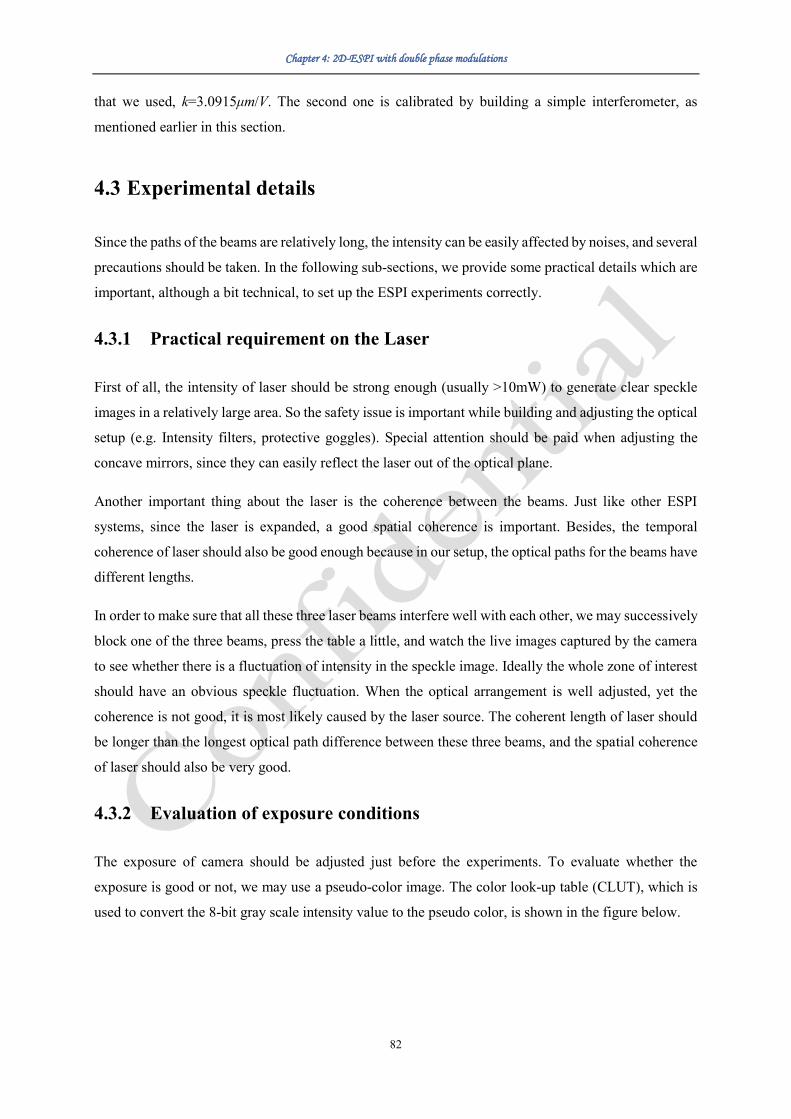
Chapter 4: 2D-ESPI with double phase modulations
82
that we used, k=3.0915μm/V. The second one is calibrated by building a simple interferometer, as
mentioned earlier in this section.
4.3 Experimental details
Since the paths of the beams are relatively long, the intensity can be easily affected by noises, and several
precautions should be taken. In the following sub-sections, we provide some practical details which are
important, although a bit technical, to set up the ESPI experiments correctly.
4.3.1 Practical requirement on the Laser
First of all, the intensity of laser should be strong enough (usually >10mW) to generate clear speckle
images in a relatively large area. So the safety issue is important while building and adjusting the optical
setup (e.g. Intensity filters, protective goggles). Special attention should be paid when adjusting the
concave mirrors, since they can easily reflect the laser out of the optical plane.
Another important thing about the laser is the coherence between the beams. Just like other ESPI
systems, since the laser is expanded, a good spatial coherence is important. Besides, the temporal
coherence of laser should also be good enough because in our setup, the optical paths for the beams have
different lengths.
In order to make sure that all these three laser beams interfere well with each other, we may successively
block one of the three beams, press the table a little, and watch the live images captured by the camera
to see whether there is a fluctuation of intensity in the speckle image. Ideally the whole zone of interest
should have an obvious speckle fluctuation. When the optical arrangement is well adjusted, yet the
coherence is not good, it is most likely caused by the laser source. The coherent length of laser should
be longer than the longest optical path difference between these three beams, and the spatial coherence
of laser should also be very good.
4.3.2 Evaluation of exposure conditions
The exposure of camera should be adjusted just before the experiments. To evaluate whether the
exposure is good or not, we may use a pseudo-color image. The color look-up table (CLUT), which is
used to convert the 8-bit gray scale intensity value to the pseudo color, is shown in the figure below.

Chapter 4: 2D-ESPI with double phase modulations
83
Figure 4-9 Color look-up table for the pseudo-color image conversion.
Experimentally, if the pseudo-color image contains mainly green/red/pink colors, and the speckle pattern
is fine and clear, then it means the adjustment of exposure is good, even though some pixels may usually
be saturated. An example is given below.
Figure 4-10 Example of pseudo-color images. (a) A bad one: the exposure is too weak. (b) A good one.
The adjustment of exposure can be done by directly adjusting the aperture of the objective lens, or by
the software FlyCapture (see figure below).

Chapter 4: 2D-ESPI with double phase modulations
84
Figure 4-11 The “camera control dialog” of FlyCapture. The important elements are highlighted by
red rectangles. More practical details are provided in the footnote①.
With the laser power and setting we use, the ambient light does not seem to be a trouble as long as a
good pseudo-color image is observed. However, if the intensity of ambient light changes, the adjustment
should be redone to obtain a good pseudo-color image again. It should be noticed that if the ambient
light is strong and the laser is too weak so that the speckle pattern is not clear, then adjusting only the
exposure is not enough; we should use a stronger laser or reduce the ambient light.
4.3.3 Data acquisition / video recording
It is recommended to save the videos temporarily in a SSD disk whose speed is higher, which is good
for recording the videos fluently. When we set the frame rate at 63 frames per second (FPS), the real
time needed to capture 63 frames may not be exactly 1 second; but as long as there is no dropped frame,
the quality of video is usually good enough. On the contrary, if we see the sign showing that there is
① Setting on FlyCapture. First, we should set the desired “Frame Rate”. Then we can just put all the
“Auto” on. When the image becomes stable, we may close all the “Auto” and capture an image to be
evaluated by the pseudo-color image. If it is good, which is often the case, then we can begin the
measurements as soon as possible; if not, we can adjust the “Exposure”, “Shutter” and “Gain” manually
until we see a good pseudo-color image. If the software adjustment reaches its limit, we can also adjust
the aperture of the objective of camera.

Chapter 4: 2D-ESPI with double phase modulations
85
dropped frame (this is usually caused by the bad contact of USB cable or the unstable performance of
computer) during the recording, it is preferable to redo the recording.
Figure 4-12 The “Capture video or image sequence” window of FlyCapture. The important elements
are highlighted by red rectangles.
When recording a video, it is necessary to choose the “uncompressed” format to avoid the loss of detail
information of speckle pattern. As shown in the following figure, the compression of images may cause
the loss of details.
Figure 4-13 Comparison of compressed and uncompressed pseudo-color speckle images. (a)
Compressed image. (b) Uncompressed image.
4.3.4 Initial phase problem
In our measuring system, when the outputs of the waveform generator are turned on manually, the phase
modulations begin; when the button “Start Recording” is clicked in the software FlyCapture, the video

Chapter 4: 2D-ESPI with double phase modulations
86
recording begins. So usually we have a non-zero initial phase for each of the two phase modulations.
Since the values of these two phase modulations are coprime numbers, there is no fixed relation between
the two initial phases. So the two initial phases should be determined one by one independently.
The best solution is to control the phase modulations and the video recording with the same computing
unit. This can be done through a microcontroller such as Arduino or via an acquisition card (e.g. NI
card). Still, the camera triggering often has a delay; yet this delay can usually be regarded as a constant
when the modulation function is fixed. The synchronization issues can then be solved by introducing
this delay in C(t) and S(t).
Another choice is to calculate the values of initial phase (as described in Section 2.3.2). Theoretically,
the fact that we have two modulated beams and one non-modulated beam interfering with each other
does not affect the final results, since the signals at different frequencies are used to calculate the initial
phase of different phase modulation functions. However, the calculated initial phase image turned out
to be very noisy, and using the average value of them can hardly lead to the best fringe image. This may
be caused by the fact that in a typical digital speckle image, there are many saturated pixels, which will
largely reduce the measurement accuracy of initial phase.
In this experiment, in order to give the best result without means of synchronization, we chose the trial
and error method. The principle is simple: we try different pairs of initial phase values before and after
deformation, and choose the phase-difference image with the best fringe visibility. This process should
be carried out for both modulation functions to get the 2D deformation field.
It should be noticed that when using the linear/sawtooth phase modulations, according to the discussion
in Section 3.1.1, a wrong guess of phase modulation will result in a constant ( )0 0gt t − added to the
final detected phase. This constant is approximately the same for every point on the plane of X-Y. So
when we make different guesses of initial phase, the changes for every point in the phase-difference
image are the same, which only makes the fringes “move” in the image without any change of fringe
visibility.
Since the phase difference is proportional to the displacement (ux or uy), a residual constant will also be
added to ux and uy. However, since we only use the derivatives of ux and uy to calculate the normal strains
(εy, εx) and shear strain (γxy), this constant will not have an influence on the final results.
x
x
u
x
=
(2.34)
y
y
u
y
=
(2.35)

Chapter 4: 2D-ESPI with double phase modulations
87
y x
xy
u u
x y
= +
(2.36)
It means that when linear/sawtooth phase modulations are used and we only care about the deformation,
then the unknown initial phase is not a problem.
When sinusoidal phase modulations are applied, and we still use the trial and error method, then
according to the discussions in Section 2.1, the sign (+/-) of the detected phases (ux and uy) may be
wrong, and there may be a phase shift of nπ ( 's s n = , n is an integer). Through the discussion
above, we already know that this phase shift of nπ will not affect the measurements of strains. However,
according to Eq. (2.34)-(2.36), the sign ambiguity of ux or uy may bring errors to the deformation
measurements. So it is necessary to check whether the final strain field is reasonable or not from the
perspective of mechanics. Otherwise, the modulators and the camera should be precisely controlled to
realize the synchronization.
4.4 Potential for 3D displacement field measurement
This method can also be extended to carry out 3D displacement field measurement without increasing
acquisition time, and without additional laser or camera. We can simply separate the laser into a fourth
coherent beam (Beam-4). This beam also hits the sample surface and interfere with Beam-1, Beam-2
and Beam-3. If the phase modulation functions for Beam-4 is F4(t), the amplitude and the initial phase
of Beam-4 are A4(x,y) and θ4(x,y) respectively, then E(x,y) becomes:
( ) ( ) ( ) ( ) ( ) ( ) ( )
( ) ( ) ( ) ( ) ( )
1 1 2 2
3 4 4
2 , 2 ,
1 2
2 , 2 ,
3 4
, , ,
, ,
c c
c c
i f t x y F t i f t x y F t
i f t x y i f t x y F t
E x y A x y e A x y e
A x y e A x y e
+ + + +
+ + +
= +
+ + (2.37)
After a small deformation, the phase of Beam-4 on the sample surface turns into θ4’(x,y):
( ) ( ) ( ) ( )44 4
2, , ,x y x y x y
= + − sn n u (2.38)
where n4 is the unit vector along illumination direction of Beam-4. We already know that:
( ) ( ) ( ) ( )33 3
2, , ,x y x y x y
= + − sn n u (2.39)
If we set
( ) ( ) ( ) ( ) ( )3 34 4 4, , , , ,C x y x y x y x y x y = − − − (2.40)

Chapter 4: 2D-ESPI with double phase modulations
88
then we have:
( ) ( ) ( )4 4 3
2, ,C x y x y
= − n n u (2.41)
If we deliberately make sure that the z component of n4-n3 is non-zero, then we know that:
( ) ( ) ( ) ( )4 , ,, ,x x y y z zu x y u x y u x yC x y h h h= + + (2.42)
where hx, hy and hz are measurable constants. Since ux(x,y) and uy(x,y) can be obtained from C1(x,y) and
C2(x,y), hz≠0, we know that uz(x,y) can be solved. This way the 3D displacement field u(x,y) is obtained.
We may also combine digital holographic interferometry (DHI) with 2D ESPI to obtain the 3D
displacement field. In this case, the forth coherent beam directly hits the CCD/CMOS matrix and
interfere with the other three beams. This time we have:
( ) ( )3 3, ,x y x y = (2.43)
Thus
( ) ( ) ( )4 3
2, ,sC x y x y
= − n n u (2.44)
Likewise, when the z component of ns-n3 is non-zero (which is usually true), the 3D displacement field
u(x,y) can be obtained.
The only problem left is to get the correct values of C1(x,y), C2(x,y) and C4(x,y). Different types of phase
modulations may be used, and appropriate modulation frequencies should be chosen for each case.
4.4.1 Linear/sawtooth phase modulations
In the case where we use linear/sawtooth phase modulations, we set:
( )4 42F t f t= (2.45)
then we have

Chapter 4: 2D-ESPI with double phase modulations
89
( )
( ) ( ) ( ) ( ) ( )
( ) ( ) ( ) ( )
( ) ( ) ( ) ( )
( ) ( ) ( ) ( )
2
3 3
1,2,3,4 1,2,4
1 2 1 1 2 2
4 2 4 4 2 2
1 4 1 1 4 4
,
, +2 , , cos , +2 ,
2 , , cos , +2 , -2
2 , , cos , +2 , -2
2 , , cos , +2 , -2
m m m m
m m
I x y
A x y A x y A x y x y f t x y
A x y A x y x y f t x y f t
A x y A x y x y f t x y f t
A x y A x y x y f t x y f t
= =
= −
+ −
+ −
+ −
(2.46)
Obviously, when f1, f2 and f4 are not equal to each other, and they are not equal to |f1-f2| or |f4-f2| or |f1-
f4|, with lock-in detections at f1, f2 and f4, we can obtain θ1(x,y)-θ3(x,y), θ2(x,y)-θ3(x,y) and θ4(x,y)-θ3(x,y)
[28]. Same procedure can be carried out to calculate θ1’(x,y)-θ3’(x,y), θ2’(x,y)-θ3’(x,y) and θ4’(x,y)-
θ3’(x,y). This way, we can get C1(x,y), C2(x,y) and C4(x,y), and thus the 3D displacement field.
The choice of is pretty simple. For example, f1=3Hz, f2=4Hz and f4=5Hz (|f1-f2|=1Hz, |f4-f2|=1Hz and |f1-
f4|=2Hz) is a good choice. Then we may set the camera frame rate at 60FPS and set the recording time
at 1 second to record every video.
4.4.2 Sinusoidal phase modulations
For the case of sinusoidal phase modulations, we set:
( )4 4sin 2F t a f t= (2.47)
Now we have:
( )
( ) ( ) ( ) ( ) ( )
( ) ( ) ( ) ( )
( ) ( ) ( ) ( )
( ) ( ) ( )
2
3 3
1,2,3,4 1,2,4
1 2 1 1 2 2
4 2 4 4 2 2
1 4 1 1
,
, +2 , , cos , + sin 2 ,
2 , , cos , + sin 2 , - sin 2
2 , , cos , + sin 2 , - sin 2
2 , , cos , + sin 2
m m m m
m m
I x y
A x y A x y A x y x y a f t x y
A x y A x y x y a f t x y a f t
A x y A x y x y a f t x y a f t
A x y A x y x y a f t
= =
= −
+ −
+ −
+ −
( )4 4, - sin 2x y a f t
(2.48)
Through similar analysis (see Section 4.2.2), we know that when J0(a)=0, the last three terms contain
|pf1±qf2|, |pf4±qf2| and |pf1±qf4| signals respectively, where p and q are positive integers.
For SPM algorithm, it is required that the last three terms do not contain f1, 2f1, f2, 2f2, f3 or 2f3 signals.
From Section 4.2.2 we know that this requirement means that: when |pf1±qf2|, |pf4±qf2| or |pf1±qf4| equals
to f1, 2f1, f2, 2f2, f3 or 2f3, the value of p or q should be relatively big (at least one of them is bigger than
6) so that Jp(a) or Jq(a) approximately equals to zero (see Figure 4-6). It is more difficult to find

Chapter 4: 2D-ESPI with double phase modulations
90
appropriate values of f1, f2 and f3 than the 2D case, but still they exist. For example, this requirement can
be satisfied by setting f1=17Hz, f2=31Hz and f3=36Hz.
For G-LIA algorithm, it is required that the last three terms do not contain any signals at integer multiples
of f1, f2, or f3 signals. This means that when |pf1±qf2|, |pf4±qf2| or |pf1±qf4| equals to mf1, mf2 or mf3 (m is
a positive integer), the value of p or q should be relatively big (at least one of them is bigger than 6).
However, this requirement is more difficult to satisfy. For example, if we still set f1=17Hz, f2=31Hz and
f3=36Hz, then we can only guarantee that p or q is bigger than 2, not 6. Knowing that J3(2.4048)≈0.2,
this set of modulation frequencies will bring some errors. So if the results are not satisfactory, it is
recommended to look for more suitable modulation frequencies, to change the algorithm, or to change
the type of modulation functions.
4.5 Results
We used a bending specimen shown in the figure below. It is a test sample fabricated by the company
HOLO 3 [52].
Figure 4-14 The bending specimen (photo taken by a camera which is not used in the experiments). By
adjusting the micrometer screw, different deformation states can be obtained. The white rectangle
represents the zone of interest.
First, we make sure that there is already an initial contact between the micrometer screw and the bending
specimen (see Figure 4-14). Then we start the two phase modulations by turning on the two channels of
the waveform generator. A short video (1 second, 63 frames per second) is recorded by the software
FlyCapture (see Section 4.3.3). Likewise, we recorded another video after turning the micrometer screw
so that the deformation state changed. We may repeat this procedure several times to record one video
at each deformation state. (It is preferred to turn the screw along the same direction without any going

Chapter 4: 2D-ESPI with double phase modulations
91
back during the measurements to avoid the hysteresis error.) By analyzing two videos at different
deformation states, we can measure the 2D displacement field.
When applying sinusoidal phase modulations described by Eq. (2.16)-(2.17) with f1=9Hz and f2=7Hz,
we successfully obtained phase images (C1 and C2), as shown in Figure 4-15. The fringe visibility is
very good; besides, very fine fringes can be observed on the left part of Figure 4-15(a,b).
Figure 4-15 Phase images (without filtering) showing the displacement field along Y-axis and X-axis
obtained with sinusoidal phase modulations. A phase difference of 2π represents a displacement
difference of about 385nm. The micrometer screw advanced 10μm and 50μm respectively along Y-axis.
The generalized lock-in detection [22,28,47] is used to process data.
From the obtained phase images (Figure 4-15), we can quantitatively measure the 2D deformation
(Figure 4-16). First, the original phase images (Figure 4-16(a,b)) were filtered (see Figure 4-16(c,d))
using the phase filtering method described in Section 3.3 (conventional 2D convolution filtering [95,96]
was used; number of iteration: 150; kernel: Gaussian blur 11×11 with a standard deviation of 0.8). Then
they are 2D-unwrapped using 2D Goldstein branch cut phase unwrapping algorithm [106,107] to get
smooth phase images, and the displacements uy and ux (Figure 4-16(e,f)) can be calculated by Eq. (2.14)

Chapter 4: 2D-ESPI with double phase modulations
92
-(2.15). Through Eq. (2.34)-(2.36), the strains εy, εx and γxy can be quantitatively measured (Figure
4-16(g,h,i)) for any choice of origins for uy and ux.
During the 2D unwrapping process, an origin point is required for each wrapped phase image. When the
real origin (the point where the displacement is known to be zero) is unknown, we may randomly choose
a point in a smooth part of the wrapped phase image as the origin. This will introduce a constant phase
shift to every point in the image, but it will not affect the measurements of strains according to Eq.
(2.34)-(2.36).

Chapter 4: 2D-ESPI with double phase modulations
93
Figure 4-16 From phase images to quantitative 2D strain field. (a,b) Unfiltered phase images (we took
the central parts of Figure 4-15(c,d) as an example). (c,d) Filtered phase images. (e,f) Displacements
uy and ux. (g,h) Normal strains εy and εx. (i) Shear strain γxy.
When applying linear/sawtooth phase modulations described by Eq. (2.7)-(2.8), similar fringes (see
Figure 4-17) are obtained, since the modulation frequencies are quite low (f1=9Hz and f2=7Hz).
However, the sawtooth approach will become much less efficient at higher speed. There are some small
differences in the fringe pattern, which are mainly due to phase noise, initial phase adjustment and the
fact that the loading processes were done manually and are not perfectly reproducible.

Chapter 4: 2D-ESPI with double phase modulations
94
Figure 4-17 Phase images (without filtering) showing the displacement field along Y-axis and X-axis
obtained with linear/sawtooth phase modulations. A phase difference of 2π represents a displacement
difference of about 385nm. The micrometer screw advanced 50μm along Y-axis. The lock-in detection
[28] is used to process data.
4.6 Conclusion
In this chapter we have applied original double phase modulations in order to perform quasi-real-time
2D-ESPI. Compared to previous reports of 2D in-plane displacement field measurement, the proposed
approach is much simpler with only one laser and one camera, yet high-quality fringes have been
obtained.
Theoretically, we can choose any two different phase modulation functions (same type with different
parameters, or even different types) for the two piezo-mounted mirrors as long as the needed signals can
be clearly separated in the frequency domain. For different choices of phase modulation functions,
appropriate algorithms should be used to separate these signals and to obtain the phase images. For
example, LIA algorithm is suitable for linear/sawtooth phase modulations, SPM algorithm is suitable
for sinusoidal phase modulations, and G-LIA algorithm is suitable for a variety of phase modulation
functions.
In this chapter, we focused on the cases when linear/sawtooth or sinusoidal phase modulations are
applied. Generally speaking, at a relative low frequency (like f<50Hz), both linear/sawtooth or
sinusoidal phase modulations can be used (the linear one has an easier algorithm, while the sinusoidal
one is better for the protection of piezo). However, at a higher frequency, it is clear that a sinusoidal
phase modulation will guarantee a much better precision in the piezo positions.

Chapter 4: 2D-ESPI with double phase modulations
95
While dealing with sinusoidal phase modulations, for the simplicity and efficiency of signal separation
in the frequency domain, it is required that J0(a)=0 (see Section 4.2.2), which coincides with the
requirement of G-LIA algorithm (see Section 1.5.3). According to the discussion in Section 1.6, we
know that when a=2.4048 rad so that J0(a)=0, G-LIA algorithm may have a better anti-noise ability.
This is an advantage for the G-LIA algorithm. However, since SPM algorithm needs less frequency
components to carry out the calculations, it is easier to find good frequencies of modulation for this
experiment, especially for the 3D measurements (see Section 4.4). So G-LIA and SPM algorithms both
have their own advantage, and the choice of algorithm should be done according to the experimental
conditions and requirements.
While a camera with moderate speed (63 frames per second) is used, the data acquisition time (1 second
for 2D information) is still more advantageous compared to some commercialized systems (e.g. 3.5
second for 3D information [55]). Obviously, this system has great potential to be operated at a high
speed while providing accurate results by using the sinusoidal phase modulation together with a high-
speed camera.
Although the relatively voluminous data may be a challenge for lower-end computers to carry out real-
time analysis at higher speed, this issue can be solved with enough computing resource or FPGA-based
(FPGA: Field-Programmable Gate Array) calculation. Last but not least, this approach has the potential
to carry out simultaneous ESPI measurement of 3D displacement field.


Chapter 5: Application of SPM in SPR detector
97
Chapter 5 Application of SPM in SPR detector
Surface plasmon resonance (SPR) is a well-known phenomenon which has been widely used for a
variety of detectors. SPR is very sensible to the change of refraction index, so there are many bio-sensors
based on SPR which can characterize molecular interactions. Apart from SPR bio-sensors, there are also
bio-sensors based on LSPR (Localized Surface Plasmon Resonance). Although SPR bio-sensor has been
developed for a longer time than LSPR bio-sensor, they both have their own advantages and
disadvantages, which will be only briefly detailed in this chapter. By combining 2D optical detectors
with SPR/LSPR, SPR/LSPR imaging (SPRi/LSPRi) has also been developed. This technique allows for
high throughput measurements (e.g. measure several different kinds of molecular interactions at the
same time). In this chapter, sinusoidal phase modulation is applied into phase-sensitive detection. A 2D
detector is used, so it also has the potential to do SPRi in the future.
5.1 Introduction to SPR
Surface plasmon resonance (SPR) is the resonant oscillation of conduction electrons at the interface
between negative and positive permittivity material stimulated by incident light. [108]
In a traditional SPR sensor (see figure below), a metal (usually gold or silver) thin film of about 40 to
50 nm when operating in the visible or NIR range, is coated on a piece of glass substrate to form the
required interface. A glass or plastic prism is then used as the coupling device: it is attached to the SPR
substrate with index-matching oil to realize the required incident angle (resonance angle θk), which is
needed to elicit the SPR. The resonance angle θk, named Kretschmann angle, is specific because
essentially, the wave vector of the p-polarized component of the incident light should be matched with
the resonance requirement. This angle, which is beyond the critical angle, is determined by the properties
of the two materials (metal and probed medium, cf. Figure 5-1). The metal thin film being fixed in
thickness and refractive index, the angle will vary with the refractive index value n(λ) of the probed
medium in the vicinity of the metal.

Chapter 5: Application of SPM in SPR detector
98
Figure 5-1 Typical set-up for an angular interrogation SPR biosensor. The darker ray impinging at a
specific angle on the detector is attenuated due to the SPR occurring at the gold/liquid interface. This
angle θk depends on the fluid refractive index in the immediate vicinity of the metal layer.
The Figure 5-1 shows a traditional angular interrogation scheme of SPR sensor. When the analytes in
the flow channel are captured on the surface of gold thin film, a small change of refractive index will
appear, thus the resonance angle will change accordingly. Since the absorption is maximum at the
resonance angle, the resonance angle θk is characterized by a reflection dip. This angle is determined
directly with such setup since the intensity of reflected light over a range of angles can be measured if a
1D detector array or a scanning detector is used. With such angle-resolved system, the change of
resonance angle can be monitored. The change in θk produced by a change of refractive index, gives
information on the analyte concentration, while the time trace θk(t) provides kinetic information on the
binding affinity between the selected probes and targets.
In addition to this scheme, there are also intensity detection scheme, wavelength interrogation scheme
and phase detection scheme. In intensity detection scheme, the incident angle is fixed at or very near θk,
and the intensity of reflected light is detected. While the dynamic range is reduced in this case, this is
sufficient if the change in θk is small or if only a threshold value needs to be determined [32]. In
wavelength interrogation scheme, a white light (or other broadband/tunable light sources) is used as
incident light. The incident angle is typically fixed, and the corresponding resonance wavelength can be
measured by analyzing the spectrum of the reflected light. In phase detection scheme, the incident angle
can be fixed or not, the important point being that the phase of the reflected light is detected.
In all these schemes, the ability to measure small refractive index change is a basic performance
indicator. From Table 5-1, we can see that the phase detection scheme has the best refractive index
resolution, and is also more convenient to do SPRi if a fixed angle angle is used, although the dynamic
range is limited in this case. Based on the literature review, our experiments, and simulation, it appears
indeed that phase detection is helpful to reach a higher resolution, if carefully selected metal thicknesses
are used.
Probed medium

Chapter 5: Application of SPM in SPR detector
99
SPR detection techniques have been commercialized for a long time. The first commercial SPR sensor
(called “Biacore”) was released by the company “Pharmacia Biosensor AB” in 1990 [109,110,111]. The
Biacore instruments (an example is shown in Figure 5-2(a)) have been evolving ever since, and the
brand of Biacore (now GE-Healthcare) is still one of the most recognized one in the field of SPR sensing
system; however, they are usually bulky.
SPR schemes Angular interrogation Wavelength interrogation Phase detection
Typical resolution 5×10⁻⁷ RIU 10-6 RIU 4×10⁻⁸ RIU
Record of resolution① 10-8 RIU [61] 10-6 RIU [112] 2.8×10⁻⁹ RIU [63]
Typical dynamic range 0.1 RIU >0.1 RIU 5×10⁻⁴ RIU
SPR imaging Difficult Difficult Convenient
Table 5-1 Brief comparison between several common schemes in SPR sensing. For the phase detection
a fixed angle is considered. Adapted from [32].
There are some other companies who focus on making portable and low-cost commercial SPR sensors.
For example, the SPR sensor called “Spreeta” was announced in 1997 (see Figure 5-2(b)). The size is
quite small and the cost is low, however additional signal processing system (including computer and
interface) is needed [113,114,115].
① Data given by our literature review. There may be better results that we did not know.

Chapter 5: Application of SPM in SPR detector
100
Figure 5-2 Commercial SPR/LSPR systems. (a) Biacore 8K [116]. (b) Spreeta [115]. (c) LiteChek [117].
If metal nanostructures are used instead of thin films, then the phenomenon of localized surface plasmon
resonance (LSPR) may happen. Just like SPR, LSPR is sensible to the change of refractive index.
Compared to SPR, LSPR is much easier to excite, so the strict angle control is no more needed [118].
This may be helpful to build compact and portable sensors.
In fact, the sensitivity of SPR is so high that the change of refractive index caused by ambient
temperature fluctuation will add noise to the signal. So for most SPR sensors, temperature control or
temperature compensation methods are needed. LSPR sensors, on the contrary, is usually less sensitive,
so LSPR sensors can hardly be affected by the ambient temperature fluctuation. However, LSPR is only
sensible to the refractive index change close to the metal surface due to stronger light concentration,
while SPR is sensitive to a larger volume (given by the penetration depth of the evanescent tail of the
impinging field). We can see that although LSPR is less sensitive to refractive index change, the
measurement efficiency of LSPR may be higher for very small targets. With further development, LSPR
sensors are hopeful to provide a resolution comparable to SPR sensors in certain cases, with the benefit
of a lesser temperature control and easier excitation.
Technically speaking, LSPR sensors are less mature than SPR sensors though. Still, there are already
commercial LSPR sensors, as shown in the Figure 5-2(c).
SPR imaging (SPRi) and LSPR imaging (LSPRi) is a research focus in recent years [58,119,120,121].
By replacing a point detector with a 2D detector matrix (e.g. CCD, CMOS), the throughput of
measurements can be largely improved. Through different functionalizations at different zones of the
metal surface and with the help of appropriate microfluidics design, several different kinds of molecular
interactions can be detected at the same time.
In this chapter, we will focus on an innovative, compact, phase sensitive SPR sensor. It should be noted
that the initial prototype and tests were notably developed in our lab by Julien Vaillant and the support
of Dr Tzu-Heng during his post-doctoral stay. This work has not yet been published. In the framework

Chapter 5: Application of SPM in SPR detector
101
of this thesis, we have considered experimentally and theoretically the possibility to add imaging
capability to the developed system, and we discuss some of the performance achievable with different
demodulation schemes. The system includes a common path interferometer and a sinusoidal phase
modulation. As will be detailed, the SPM is achieved through the combined use of a current-modulated
Vertical Cavity Surface Emitting Laser (VCSEL) and an anisotropic crystal. A CMOS camera is used
as detector, showing the potential to do SPRi in the future.
5.2 Principle of phase modulation through wavelength modulation
Phase modulation through wavelength modulation can be achieved when an unbalance exists between
signal and reference arm. This approach may enable low-cost and high-speed operation because, as will
be shown here, only a small wavelength change is required and laser diode can be modulated at very
high frequency. Some practical issues limit the use of this technique, mainly related to the wavelength
stability; but this issue is mostly overcome in the developed system presented in the forthcoming
sections.
In our setup, the phase modulation is obtained via an injection current modulation of the laser source.
This current modulation entails a small wavelength modulation which can be converted into a phase
modulation if the signal and reference beams have unbalanced paths. In order to modulate the current
(and therefore obtain a phase modulation), we need to modulate the input voltage.
We know that for a VCSEL, in the vicinity of the operating voltage U0, the output wavelength λ of
VCSEL approximately will exhibit a linear relationship with the input voltage U:
U = (3.1)
where τ is a constant. When applying the operating voltage U0, we have the expression of operating
wavelength λ0:
0 0U = (3.2)
If we define that:
0
0U U U
= − = −
(3.3)
Then we get:
U = (3.4)

Chapter 5: Application of SPM in SPR detector
102
If we separate the laser beam in two beams, and the optical path difference is L, then we have the
resulting phase difference κ:
2 L
= (3.5)
If we take the differential on both sides, then we have:
2
2 Ldd
−= (3.6)
When applying the operating voltage U0, we have the phase difference κ0:
0
0
2 L
= (3.7)
We define that:
0 = − (3.8)
When the wavelength change Δλ is small, approximately we have:
2
0
2 L
− = (3.9)
So that
0 0 02 2
0 0
2 2L LU
− −= + = + = + (3.10)
By defining a coefficient:
2
0
2 L
−= (3.11)
We can express this approximation by:
U = (3.12)
In the case of SPM, this equation gives an expression for the phase modulation depth, i.e. a= χΔU for a
given sine voltage modulation U(t)=Uo+ΔU.sin(ωt). It shows that when the amplitude of voltage
modulation is small, then the phase modulation depth is approximately proportional to the voltage
change.

Chapter 5: Application of SPM in SPR detector
103
In practice, we used a VCSEL emitting at around λ0=670nm. If we suppose that L=1mm, then we may
make a simulation to see the precision of this approximation. The results are shown by the following
figures:
Figure 5-3 Phase difference (wrapped) caused by the modulation of wavelength.
Figure 5-4 Error of the approximation described by Eq. (3.9).
Figure 5-3 shows that when the wavelength is tuned by 1nm (from 669.5nm to 670.5nm), the error of
approximation is small; besides, the phase difference changes for more than 4π in this zone, which is
big enough to carry out most phase modulation functions. From Figure 5-4, we can see that in this range
of modulation, the maximum error is about 5×10⁻³rad, which is often tolerable.

Chapter 5: Application of SPM in SPR detector
104
In practice, in order to measure , we may directly apply a slow linear phase modulation to the
VCSEL and measure the period of the interference signal. For example, with our setup, we obtained
experimentally that 8.6 /mV rad .
When a sinusoidal phase modulation with the amplitude a=3.8317rad is needed, which corresponds to
Δκ=±3.8317rad at maximum, according to Eq. (3.12) and 8.6 /mV rad , we can get ΔU≈±33mV
at maximum, thus we can set 66mV as the peak-to-peak value of VCSEL voltage modulation. This value
should also be adjusted by observing Lissajous curves experimentally, which will be discussed in
Section 5.4, to guarantee the precision of the measurements.
5.3 Phase extraction in wavelength modulated interferometers
When a voltage modulation is applied to the VCSEL, the output power/intensity changes too, which can
be described by Eq. (1.40). To extract the phase information while using sinusoidal phase modulation,
three algorithms may be used.
The first one is the modified SPM algorithm (see Section 2.3.1). However, the coefficient μ representing
the intensity modulation should be known. It can be easily measured by applying a slow linear voltage
modulation and monitoring the output power/intensity (no interferometry). Some simple tests are done
to prove the feasibility of this method (see Section 5.4).
The second one is the modified f-G-LIA algorithm (see Section 2.3.3). In our experiments, μ is relatively
small and the amplitude of phase modulation a=3.8317rad can be achieved. So this algorithm can be
simplified into f-G-LIA algorithm (see Section 1.5.4). This method is used to carry out detections of
refractive index change (see Section 5.4).
The third one is the modified integrating bucket algorithm (see Section 2.3.4). This method requires
precise exposure time control, which is beyond the scope of this thesis.
5.4 Experiments
The operation principle is described in this part through two simplified, preliminary, setups made in this
thesis to test the phase extraction methods.

Chapter 5: Application of SPM in SPR detector
105
5.4.1 Preliminary setup: test of the algorithms
Before using the CMOS camera as detector, we test the feasibility of modified SPM/f-G-LIA algorithms
by using a photo detector. A common path interferometer, which can hardly be affected by external
vibrations or noises, is built. The setup is shown in the figure below.
Figure 5-5 Preliminary setup for testing the algorithms.
The initial polarization of laser is at around 45° with respect to the vertical axis. Then the laser passes
through a birefringent crystal YVO4, which leads to an optical path difference between the 0° and the
90° polarization components of laser, although the geometrical paths are the same for them. This optical
path difference due to the crystal anisotropy can be seen as a constant L (see Eq. (3.5)). Thus the phase
modulation method described by Section 5.2 can be carried out by modulating the input voltage to the
VCSEL. A polarizer at around 45° is put after the YVO4 crystal to make the 0° and 90° laser components
interfere with each other. Then the interference signal is captured by the single photo detector. The
software LabVIEW is used to control the input voltage to the VCSEL, to obtain the signal from photo
detector, and to process the data, with the help of a NI card.

Chapter 5: Application of SPM in SPR detector
106
In order to test the system setting, we add a “fake” phase change, via a small triangular voltage
modulation, which is added to the sinusoidal modulation to cause a triangular phase change (see Eq.
(3.11)-(3.12)). If the frequency of this triangular signal is much smaller than the sinusoidal phase
modulation, then during each sampling / each calculation for one phase value, the triangular signal can
be seen as a constant. Therefore, if our measuring method works fine, this triangular phase change can
be obtained.
Such simple tests are done with the modified SPM/f-G-LIA algorithms. The results are shown in the
figure below:
Figure 5-6 Measuring a sawtooth phase change in the common path interferometry with different
algorithms. (a) With modified SPM algorithm; (b) With f-G-LIA algorithm.
The retrieved phase is shown in red. From the figure above, we can see that these two algorithms both
give precise results. There is a small delay in both of them, which is caused by the data transmission and
processing. Since this delay is small and constant, it is not a problem for most measurements.
Calibration
The input voltage to the VCSEL can be calibrated using the Lissajous curve beforehand. We take the
case of the f-G-LIA algorithm as an example: if we plot all the possible points ,X Y
M N
(see Section
1.5.4 for definitions of X, Y, M and N) in a Cartesian coordinate system, then according to Eq. (0.53),

Chapter 5: Application of SPM in SPR detector
107
we can get a perfect circle if all the measurements are precise. If the circle is not round enough, then the
input voltage to VCSEL should be adjusted.
By varying the added phase change in a range larger than 2π, we can get the Lissajous curves, as
exemplified in the figure below:
Figure 5-7 Lissajous curves while using different algorithms after calibrations①. (a) Modified SPM
algorithm; (b) f-G-LIA algorithm.
Generally speaking, the two Lissajous curves in Figure 5-7 are both tolerable, and similar good results
using these two algorithms have been shown in Figure 5-6. We can also see from Figure 5-7 that the
Lissajous curve given by modified SPM algorithm (see Section 2.3.1), which takes the non-zero value
of μ into account, is closer to a perfect circle than the one given by f-G-LIA algorithm (see Section
1.5.4), which requires that μ≈0 (or small enough). The non-perfect calibrations may also be one of the
reasons for that. It should be noticed that with the modified f-G-LIA algorithm (see Section 2.3.3), the
non-zero value of μ can also be taken into account. So theoretically speaking, the modified
SPM/f-G-LIA algorithms are preferred. However, f-G-LIA is simpler in practice, and when the
calibration is nicely done, it can also give very good results, as shown in Figure 5-6. Since our primary
goal is to prove the feasibility of this method, we choose to use the f-G-LIA algorithm for the following
experiments.
5.4.2 Phase-sensitive SPR sensor
A homemade SPR sensor is shown in the following figure:
① The calibrations may not be perfectly done, since they are performed manually.
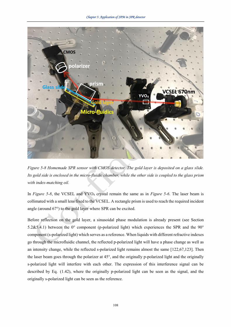
Chapter 5: Application of SPM in SPR detector
108
Figure 5-8 Homemade SPR sensor with CMOS detector. The gold layer is deposited on a glass slide.
Its gold side is enclosed in the micro-fluidic chamber, while the other side is coupled to the glass prism
with index-matching oil.
In Figure 5-8, the VCSEL and YVO4 crystal remain the same as in Figure 5-6. The laser beam is
collimated with a small lens fixed to the VCSEL. A rectangle prism is used to reach the required incident
angle (around 67°) to the gold layer where SPR can be excited.
Before reflection on the gold layer, a sinusoidal phase modulation is already present (see Section
5.2&5.4.1) between the 0° component (p-polarized light) which experiences the SPR and the 90°
component (s-polarized light) which serves as a reference. When liquids with different refractive indexes
go through the microfluidic channel, the reflected p-polarized light will have a phase change as well as
an intensity change, while the reflected s-polarized light remains almost the same [122,67,123]. Then
the laser beam goes through the polarizer at 45°, and the originally p-polarized light and the originally
s-polarized light will interfere with each other. The expression of this interference signal can be
described by Eq. (1.42), where the originally p-polarized light can be seen as the signal, and the
originally s-polarized light can be seen as the reference.
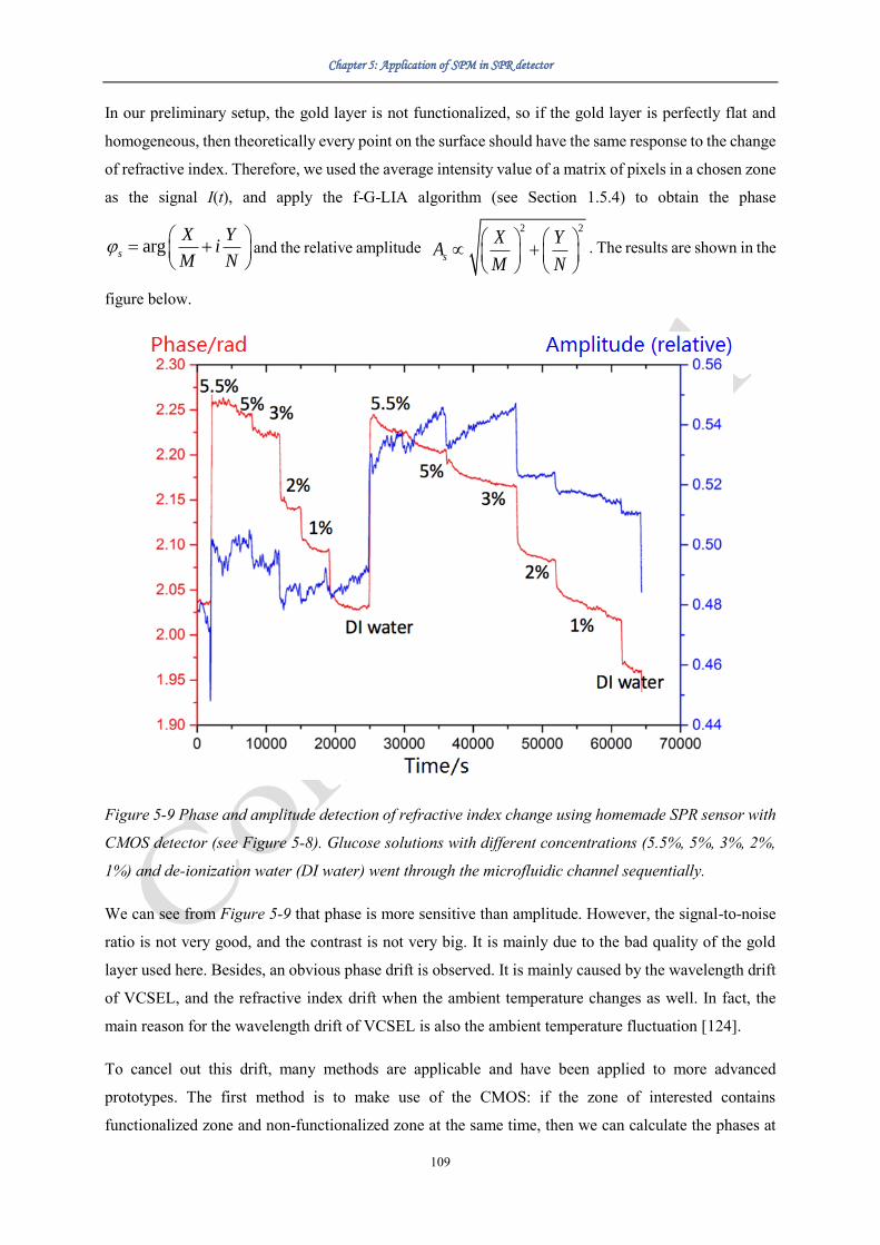
Chapter 5: Application of SPM in SPR detector
109
In our preliminary setup, the gold layer is not functionalized, so if the gold layer is perfectly flat and
homogeneous, then theoretically every point on the surface should have the same response to the change
of refractive index. Therefore, we used the average intensity value of a matrix of pixels in a chosen zone
as the signal I(t), and apply the f-G-LIA algorithm (see Section 1.5.4) to obtain the phase
args
X Yi
M N
= +
and the relative amplitude
2 2
s
X YA
M N
+
. The results are shown in the
figure below.
Figure 5-9 Phase and amplitude detection of refractive index change using homemade SPR sensor with
CMOS detector (see Figure 5-8). Glucose solutions with different concentrations (5.5%, 5%, 3%, 2%,
1%) and de-ionization water (DI water) went through the microfluidic channel sequentially.
We can see from Figure 5-9 that phase is more sensitive than amplitude. However, the signal-to-noise
ratio is not very good, and the contrast is not very big. It is mainly due to the bad quality of the gold
layer used here. Besides, an obvious phase drift is observed. It is mainly caused by the wavelength drift
of VCSEL, and the refractive index drift when the ambient temperature changes as well. In fact, the
main reason for the wavelength drift of VCSEL is also the ambient temperature fluctuation [124].
To cancel out this drift, many methods are applicable and have been applied to more advanced
prototypes. The first method is to make use of the CMOS: if the zone of interested contains
functionalized zone and non-functionalized zone at the same time, then we can calculate the phases at

Chapter 5: Application of SPM in SPR detector
110
these two zones respectively and make the subtraction. The second method is to compensate only the
wavelength drift of VCSEL: by inserting a beam-splitter between YVO4 and the prism in Figure 5-8,
we can measure the initial phase difference between the p-polarized and s-polarized light before being
reflected by the gold layer, then we can subtract this initial phase from the measured phase in real time.
This second method has been proved to be very effective. Fig. 6-10 shows the results of an experiment
done in our research group to prove this point: the second method is used to cancel out the phase drift,
a simple photodiode is used to replace the CMOS matrix, angular interrogation mechanism is added,
and a commercial SPR chip is coupled on a 45° prism, while the phase modulation method and phase
retrieval method remain the same.
Figure 5-10 Angular interrogation SPR sensor with phase and intensity detection. Sinusoidal phase
modulation is carried out by VCSEL wavelength modulation (see Section 5.2). f-G-LIA algorithm (see
Section 1.5.4) is used to extract the phase information. A commercial SPR chip is used without any
microfluidics. (a) Phase response to angle change. (b) Intensity response to angle change.
As shown in Figure 5-10(b), at SPR angle (around 44.3°), the intensity is almost zero, which proves that
the quality of this SPR chip is so good that the electromagnetic coupling is very effective. In Figure
5-10(b), we can see that the phase measurement is very stable and there is a quasi-vertical drop of phase
at SPR angle, which proves the efficiency of our method to compensate the wavelength drift of VCSEL,
as well as the feasibility of our phase detection method.
In Figure 5-10, the small zone around SPR angle where we have a quasi-vertical drop of phase can be
called “phase-sensitive zone”. We can make use of this zone to do highly sensitive SPR phase detections.
If we fix the angle at the center of this zone (SPR angle), then when a tiny change of refractive index

Chapter 5: Application of SPM in SPR detector
111
takes place on the gold surface, a big phase difference can be detected. The only drawback of using this
zone is that: the light intensity of signal (p-polarized light) remains very small in this zone, while the
intensity of reference (s-polarized light) is as strong as usual, which may result in a loss of signal-to-
noise ratio to some extent. But its influence seems to be limited, since in Figure 5-10, we did not get
unnormal phase values in this phase-sensitive zone.
For all the experiments in this section, the software LabVIEW was used to control all the
outputs/inputs/calculations/displays. The advantage is that the phase modulation and intensity detection
(e.g. capturing pictures for the camera) can usually be synchronized easily. Thus we do not need to
worry about the initial phase problem (see Section 2.1).
5.5 Perspective: Combining shearing interferometry with SPRi
From the discussions in Sections 5.1 & 5.4.2, we know that the ambient temperature fluctuation may
affect the precision of SPR measurements, and two methods were proposed to solve this problem.
In this section, we propose another method which is inspired by the shearography technique: to make
SPR imaging with the help of shearing interferometry to compensate these errors, with the benefit of
using a single polarization component. First of all, we need a shearing element to make a shearing to the
original image and to superpose these two images. A modified cube beam splitter is proposed to achieve
this function. The principle is shown in the figure below:
Figure 5-11 A modified cube beam splitter working as the shearing element. The upper side and the left
side of the beam splitter are coated with metal so that the light can be efficiently reflected. If the optical
paths are the same for the separated beams (this kind of beam splitter is represented by the blue lines),
then there will no shearing between the two beams, as shown by the red lines. If one side of the beam

Chapter 5: Application of SPM in SPR detector
112
splitter is thicker (see the orange lines) than the other one, then the laser beam reflected by the thicker
side (see the pink lines) will be parallel but shifted away from the other one.
Through simple geometric derivation, we deduced that the shifted beam (pink) and the other beam (red)
are parallel in the end with a distance:
2 sins d = (3.13)
Also, we can obtain the optical path difference:
2 cosL d = (3.14)
Obviously, s and L can be easily adjusted by changing d and δ.
When an expanded and collimated laser beam is incident, this shearing is applicable to the whole beam,
resulting in an image of shearing interferometry. The following figure shows the proposed shearing SPR
imaging system:
Figure 5-12 Combination of shearing interferometry and SPR imaging.
When the incident angle to the prism is fixed, presuming that the incident collimated beam is
homogeneous, we have the functions A(n) and φ(n) to represent the amplitude and phase of reflected
light (n is the refractive index). At different zones of functionalization, the values of n are often different.
For example, in Zone-1 and Zone-2, respectively we have:
( ) ( )( )12
1 1
i ft nE A n e
+= (3.15)
( ) ( )( )22
2 2
i ft nE A n e
+= (3.16)
At the places where Zone-1 is not overlapped with Zone-2, the light intensity can be expressed as:

Chapter 5: Application of SPM in SPR detector
113
( )2 2
11 1 1 14I E E A n= + = (3.17)
( )2 2
22 2 2 24I E E A n= + = (3.18)
At the places where Zone-1 is overlapped with Zone-2, the light intensity can be expressed as:
( ) ( ) ( ) ( ) ( ) ( )( )2 2 2
12 1 2 1 2 1 2 1 22 cosI E E A n A n A n A n n n = + = + + − (3.19)
When the ambient temperature changes, if we suppose this change lead to the same refractive index
change nt in Zone-1 and Zone-2, then we have:
( ) ( )( )12
1 1' ti ft n n
tE A n n e + +
= + (3.20)
( ) ( )( )22
2 2' ti ft n n
tE A n n e + +
= + (3.21)
( ) ( ) ( ) ( ) ( ) ( )( )2 2 2
12 1 2 1 2 1 2 1 2' ' ' 2 cost t t t t tI E E A n n A n n A n n A n n n n n n = + = + + + + + + + − + (3.22)
As discussed in Section 5.4.2, for SPR phase detection, we make use of the “phase-sensitive zone”,
where the phase changes rapidly and almost linearly, and the intensity changes slowly (see Fig. 6-10).
So approximately we have:
( ) ( )1 1tA n n A n+ (3.23)
( ) ( )2 2tA n n A n+ (3.24)
( ) ( ) ( ) ( )1 2 1 2t tn n n n n n + − + − (3.25)
Thus
12 12'I I (3.26)
Which means that the influence of ambient temperature change can be compensated.
The intensity I12 is mainly determined by the phase difference ( ) ( )1 2n n − , making this system able
to do phase-sensitive detections. Besides, A(n1) and A(n2) can be measured where Zone-1 is not
overlapping with Zone-2. (See Eq. (3.17)-(3.18)) A simulation of a possible shearing image is shown
in the figure below:

Chapter 5: Application of SPM in SPR detector
114
Figure 5-13 A possible shearing image made by simulation. It is supposed that the round zone in the
middle (Zone-2) is functionalized and that the analyte is attached to its surface evenly, while the other
part (Zone-1) is only non-functionalized gold layer. A beam-splitter of 50/50 is used, and a pure
horizontal shear is realized.
Obviously, Figure 5-13 is the simplest case for SPR imaging. SPR chips with different functionalization
zones can be used in this method, as long as the shearing distance s (see Figure 5-11) is well controlled.
5.6 Conclusion
In this chapter, we have analysed the possibility to combine SPM with SPR sensor as preliminary tests
for phase sensitive SPRi. These preliminary experiments were done to prove the feasibility of this idea.
A CMOS is used as detector to show the possibility of doing SPR imaging in the future. The initial phase
problem (see Section 2.1) is solved by using LabVIEW to control the whole measuring system.
Generally speaking, in our experiments, the goal of combining sinusoidal phase modulating
interferometer and SPR sensor is to make a cheap, simple, compact, robust yet high-precision SPR
detector. By using VCSEL as the light source, the cost can be lowered; besides, the size of VCSEL is
small, and the input voltage is low (less than 5V), which is practical for the fabrication of compact and
portable devices in the future. Phase detection is used to improve the precision. By simply modulating

Chapter 5: Application of SPM in SPR detector
115
the input voltage to the VCSEL, phase modulation can be realized, which reduce the cost as well as the
complexity of measuring system. Sinusoidal phase modulation was applied to guarantee the precision
of modulation, and corresponding algorithms for signal processing have been developed to extract
information. Simple yet effective temperature compensation methods have been proposed to further
improve the stability and precision of the measuring system.
Based on this system, many methods may be applied to improve its performance in the foreseeable
future. For example, we may functionalize the gold surface differentially at different zones to realize
SPR imaging, use nanostructures (e.g. Graphene–MoS2 hybrid nanostructures [123]) to enhance the
sensitivity of SPR sensor, use holograph/grating to realize the coupling of the incident light with the
surface plasmon of the gold layer, combine SPR imaging with shearing interferometry (see Section 5.5),
use LSPR chips instead of SPR chips, combine angle interrogation with phase detection in SPR imaging,
etc.

General conclusion and perspectives
116
General conclusion and perspectives
General conclusion
Phase modulation techniques can be applied in almost every interferometric measuring systems.
Basically, by applying phase modulations, the number of sampling for each measurement increases, thus
the measurement precision can be greatly improved, and the phase ambiguity problem can also be
solved. In order to provide new possibilities for simple, cheap, reliable and precise interferometric
measurements, we have studied the signal of phase modulating interferometer theoretically and
experimentally. Sinusoidal phase modulation was specifically considered because such modulation is
typically affordable and it can be accurately achieved even at high frequency.
Sinusoidal phase modulation has been applied in holography and holographic interferometry. (f)-G-LIA
algorithm is used to retrieve phase information, and the obtained results are similar to the traditional
SPM algorithm. Besides, two linear/sawtooth or sinusoidal phase modulations are applied in an
innovative 2D-ESPI setup, making it possible to do simultaneous 2D displacement field measurement
with a single laser and camera. Sinusoidal phase modulation has also been applied to phase-sensitive
SPR sensor. Several methods to compensate the ambient temperature fluctuation have been proposed.
The feasibility has been proved by a preliminary setup.
In Chapter 1, we focused on the basic principles and mathematical expressions of interference signal.
Several phase-shifting and phase modulation techniques were introduced, and the corresponding
algorithms were presented. We highlighted the newly proposed (f-)G-LIA algorithm, and compared its
application in SPM interferometer with the traditional SPM algorithm.
In Chapter 2, two practical problems were considered: the initial phase problem, which is caused by the
non-synchronized detection and modulation, and the intensity modulation problem, which occurs in
most laser diodes when applying an injection current modulation for doing SPM. The modulated signal
was analysed in the frequency domain, and the mathematical solutions for these problems in different
algorithms have been deduced.
In Chapter 3, sinusoidal phase modulation was applied in a homemade co-axis lens-less DH/DHI system.
A reasonable spatial resolution (32 LP/mm) was obtained, and precise out-of-plane rotation
measurements (with a sensitivity better than 0.004°) have been realized. SPM algorithm and (f-)G-LIA
General conclusion and perspectives
117
algorithm were applied to retrieve the phase information. The results given by these two algorithms have
been compared, and it can be concluded that the performance of (f-)G-LIA is only slightly superior for
the investigated phase modulation depth.
In Chapter 4, an innovative 3-beam ESPI system was built to carry out simultaneous 2D in-plane
deformation measurements. Two modulations with different frequencies have been added to the two
beams respectively. The displacement field along X-axis and Y-axis can be separated in the frequency
domain efficiently. The fringe visibility is very good for both directions. Sinusoidal phase modulation
and linear/sawtooth modulations have been tested and proved to be applicable. The possible extension
of this method to carry out 3D measurements has been discussed.
In Chapter 5, the use of sinusoidal phase modulation in phase-sensitive SPR sensor was discussed. More
precisely, a common-path design using YVO4 crystal combined with wavelength modulated VCSEL
was considered for its high stability potential and possible high modulation frequency. The modified
SPM algorithm and the f-G-LIA algorithm have been firstly tested without SPR chip. Then a preliminary
experiment using a SPR chip and a CMOS matrix was done to show the feasibility of this method. The
idea of applying shearing interferometry into SPRi was also proposed.
Perspectives
Smart detector using sinusoidal phase modulation
For SPM interferometers, the relatively complex data processing may limit the maximum measurement
speed and make it impossible to realize real-time measurements with lower-end computers.
Nevertheless, we noticed that a new kind of camera called “lock-in camera” has been proposed and
fabricated, which was originally developed for high-speed low coherence interferometry
[125,126,127,128]. Inspired by such lock-in camera, we propose to realize SPM camera by combining
SPM interferometer with smart detector array. The principle is shown by the figure below:

General conclusion and perspectives
118
Figure C-1 Flowchart of the working principle for one smart pixel in SPM camera.
We may use the waveform generator to generate two synchronized voltage signals, asin(ωt) and
acos(2ωt), where a is a positive constant representing the amplitude of phase modulation. Then the
signal of asin(ωt) is used to modulate the piezoelectric actuator (or wavelength modulation); the signals
asin(ωt) and acos(2ωt) as well as the light intensity signal I(t) enter the smart detector array to make
analogue calculations. The operations described by Eq. (0.28)-(0.29), which used to be the most time-
consuming steps, are carried out through this analogue signal treatment. [125,126] Then the images of
X and Y described by Eq. (0.28)-(0.29) are directly transferred to the computer at a speed comparable
to the frame rate of camera, and the computer can easily calculate and show the results through Eq.
(0.32) in real time. Obviously, the required time for each measurement can be greatly shortened, thus
the time issue of data acquisition and data processing should be efficiently solved.
Another advantage is that the synchronization of the system is also done automatically: the same signal
asin(ωt) is used to control the piezoelectric actuator and to make analogue calculations, and the two
outputs of waveform generator (asin(ωt) and acos(2ωt)) can usually be synchronized easily.
In a word, smart detector and SPM interferometer seems to be a perfect match even if the cost of such
smart detector may be prohibitive for a number of applications. Ideally, this approach should be certainly
pursued as a perspective beyond this thesis work.
Automatic control of measuring systems
Since the initial phase has been solved mathematically and experimentally, most of the experiments
presented in this thesis do not have synchronization control (in some cases modulation and detection
were synchronized though, especially when a point detector is used). However, in order to improve the

General conclusion and perspectives
119
measurement precision and make automatic measurements in the future, automatic control will become
necessary. The goal is to accomplish the measurements only by using a single software in a computer
with the least manual operation after properly adjusting the optical setup. Generally speaking, this
automatic control may include: synchronization and control of the camera and modulation, calibration,
processing, image filtering, etc.
As discussed before, smart detectors may be used to fulfil the synchronization and to greatly increase
the measuring speed. Additional algorithms are also needed to find automatically the position of sample
/ find the position with the best fringe visibility in the reconstruction process of DH/DHI, as well as to
find the SPR angle in SPR sensor. To control the incident angle in SPR setup, the automatic control may
be carried out with stepping motor (which is done on recent prototypes in our group using
microcontrollers) and appropriate algorithms (to find the Kretschmann angle, to realize the
measurements at different angles, etc.).
Final comments
In this thesis, several advances based on phase modulation techniques have been proposed; besides,
linear/sawtooth and sinusoidal phase modulations have been analyzed intensively. However, there are
also many other kinds of phase modulation functions, which may be used to suppress the noise in the
interferometric signal at different frequencies, as discussed in Section 1.6. Generally speaking, a good
choice of phase modulation function can help to improve the anti-noise ability, precision, stability of a
measuring system, and even the service lifetime of modulators as well. Therefore, the choice of the
phase modulation functions, and the related parameters such as the phase modulation depth, etc. should
be considered carefully for each application.
In fact, there are many kinds of modulators in interferometry: piezo-mounted mirror, piezoelectric
optical fiber stretcher, liquid crystal on silicon-spatial light modulator (LCOS-SLM), photoelastic
modulator (PEM), free-space electro-optic modulators, laser diode with tunable wavelength, etc. Such
modulators that have different properties and different costs, can be matched with different phase
modulation functions to meet actual needs. It is important to wisely choose the type of modulator, the
type of modulation function and phase-retrieval algorithm according to the modulation frequency, and
other parameters such as the required modulation precision and range, the noise characteristics, the
wavelength of the laser or the desired cost. A well-balanced equilibrium between all these factors is
desirable to achieve high performance and cost efficient interferometric system for a considered
application.


Résumé en français
121
Résumé en français
Dans cette thèse, nous nous intéressons aux signaux interférométriques à modulation de phase continue,
dans le but de développer des dispositifs de détections performants et originaux pour des applications
en mécanique et en optique.
Nous présentons d'abord plusieurs des techniques de modulation et démodulation employées dans ce
contexte. Nous nous focalisons sur les modulations de phase sinusoïdales (SPM), qui sont
particulièrement avantageuses pour les dispositifs de modulations les plus largement accessibles (e.g.
modulateurs piézoélectriques, électro-optiques, ...). Nous proposons en particulier des solutions au
problème de synchronisation lors du processus de démodulation ainsi qu'au problème éventuel de
modulation d'amplitude concomitante à la modulation SPM.
Ces techniques de démodulations sont ensuite appliquées à trois dispositifs expérimentaux développés
au cours de cette thèse. Il s'agit d'abord d'un dispositif d’holographie digitale compact sans lentille,
mettant en œuvre une modulation SPM simple, pour de l'imagerie et de la mesure de déplacement sans
lentille. Nous utilisons ensuite une technique de modulation à double fréquence pour réaliser des
mesures bidimensionnelles de champ de déformation, à l'aide d'un dispositif ESPI (interférométrie de
speckle électronique) original. Cette approche permet une mesure simultanée selon les 2 directions du
plan à l'aide d'un seul système de laser et caméra. Finalement, nous présentons un instrument de type
SPR (Surface Plasmon Resonance) compact mettant en œuvre une détection interférométrique de type
SPM à modulation de longueur d'onde, dans lequel la modulation d'amplitude est prise en compte avec
succès.
1. Algorithmes de récupération de phase
Dans le cas d’une interférence entre deux ondes planes polarisées selon la même direction, l’intensité
en un point où les deux champs se superposent s’écrit :
( )2 2 2= 2 cosr s r s r s r sI E E A A A A + = + + − (1)

Résumé en français
122
Où apparaissent As et ϕs l’amplitude et la phase du champ signal, qui en notation scalaire complexe
s’écrit :
( )2 si ft
s sE A e +
= (2)
Où t et f sont le temps et la fréquence de la lumière respectivement. Ar et ϕr sont l’amplitude et la phase
du champ considéré comme référence, qui en notation scalaire complexe s’écrit également:
( )2 ri ft
r rE A e +
= (3)
Nous pouvons définir la différence de phase qui est mesurable:
s s r = − (4)
Alors notre première équation devient:
( )2 2 2 cos -r s r s sI A A A A = + + (5)
Afin de mesurer s sans ambiguïté, des méthodes de « décalage de phase » ont été introduites,
consistant à ajouter une phase contrôlable r à la lumière de référence, l'intensité se transforme alors
en:
( )2 2 2 cosr s r s r sI A A A A = + + − (6)
En affectant à r certaines des valeurs différentes, s peut être mesurée sans ambiguïté. Pour
augmenter la précision, Nous pouvons également faire une modulation de phase continue ( )r t .
L'intensité de la lumière devient donc un signal temporel I(t):
( ) ( )( )2 2 2 cosr s r s r sI t A A A A t = + + − (7)
Pour une modulation de phase linéaire simple:
( ) 0 02r t t f t = = (8)
Dans ce cas une détection synchrone (LIA : Lock-in amplifier) peut être utilisée pour démoduler le
signa, c’est-à-dire retrouvé l’amplitude et la phase φs du champ signal. D’abord, nous définissons deux
fonctions C(t) et S(t) :
( ) ( )0cosC t t= (9)
( ) ( )0sinS t t= (10)
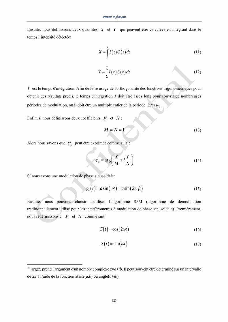
Résumé en français
123
Ensuite, nous définissons deux quantités X et Y qui peuvent être calculées en intégrant dans le
temps l’intensité détéctée:
( ) ( )0
T
X I t C t dt= (11)
( ) ( )0
T
Y I t S t dt= (12)
T est le temps d'intégration. Afin de faire usage de l'orthogonalité des fonctions trigonométriques pour
obtenir des résultats précis, le temps d'intégration T doit être assez long pour couvrir de nombreuses
périodes de modulation, ou il doit être un multiple entier de la période 02 / .
Enfin, si nous définissons deux coefficients M et N :
1M N= = (13)
Alors nous savons que s peut être exprimée comme suit①:
args
X Yi
M N
= +
(14)
Si nous avons une modulation de phase sinusoïdale:
( ) ( ) ( )sin sin 2r t a t a ft = = (15)
Ensuite, nous pouvons choisir d'utiliser l’algorithme SPM (algorithme de démodulation
traditionnellement utilisé pour les interféromètres à modulation de phase sinusoïdale). Premièrement,
nous redéfinissons c, M et N comme suit:
( ) ( )cos 2C t t= (16)
( ) ( )sinS t t= (17)
① arg(z) prend l'argument d'un nombre complexe z=a+ib. Il peut souvent être déterminé sur un intervalle
de 2π à l’aide de la fonction atan2(a,b) ou angle(a+ib).

Résumé en français
124
( )2M J a= (18)
( )1N J a= (19)
Et alors
args
X Yi
M N
= +
(20)
L’algorithme dit G-LIA (LIA généralisé), récemment introduit dans notre laboratoire, peut être utilisé
pour traiter de nombreux types de fonctions de modulation de phase, dont la fonction de modulation de
phase sinusoïdale. Pour tout type de fonction de modulation de phase ( )r t , C(t) et S(t) sont définis
comme suit:
( ) ( )( )cos rC t t= (21)
( ) ( )( )sin rS t t= (22)
Pour la modulation de phase sinusoïdale décrite par Eq. (15), M et N sont ainsi redéfinis:
( )01 2M J a= + (23)
( )01 2N J a= − (24)
Enfin, s peut être obtenu:
args
X Yi
M N
= +
(25)
Néanmoins, en raison de la présence d’une composante continue dans I(t) et dans C(t), cettte méthode
ne fonctionne sans précaution particulière que si on impose ( )0 0J a = , de manière à supprimer la
composante continue de C(t).
Pour s’affranchir de cette contrainte, l’algorithme f-G-LIA (algorithme G-LIA avec filtre) peut être
utilisé. Tout d'abord ( )I t passe par un filtre DC avant d’être traité. M doit alors être redéfini
comme:
( ) ( )2
0 01 2 2M J a J a= + − (26)

Résumé en français
125
Les autres étapes de l'algorithme f-G-LIA sont les mêmes que l'algorithme G-LIA. Évidemment quand
( )0 0J a = , l'algorithme f-G-LIA et l'algorithme G-LIA sont équivalents.
Cependant, deux problèmes peuvent généralement augmenter la complexité du processus de
démodulation. Le premier est la phase initiale non nulle de la modulation de phase, qui se produit lorsque
les modulateurs (comme les actionneurs piézo-électriques) et l’acquisition ne sont pas synchronisés. Le
second est lié à l’existence d’une certaine modulation d'intensité due à la modulation de phase. Ce
problème se produit souvent lorsque la modulation de phase est assurée par une modulation de la
longueur d'onde de la source laser (comme un VCSEL). En tenant compte de ces deux problèmes, le
signal d'interférence d'un interféromètre à modulation de phase sinusoïdale devient:
( ) ( )( ) ( )2 2 2 cos sin 1 sinr s r s sI t A A A A a t a t = + + + − + + (27)
Où θ est la phase initiale de modulation, μ est la profondeur de modulation d’amplitude dont la valeur
dépends directement de la profondeur de modulation en phase a désirée et des caractéristiques du laser.
En utilisant l'expansion de Jacobi-Anger et les identités trigonométriques, nous pouvons analyser le
signal I(t) dans le domaine fréquentiel:
( ) ( )( ) ( )
( ) ( )( ) ( )( )
( )
( )
2 2
1
2,4,... 3,5
0
,...
0,2,...
1,3,...
2 cos sin 1 sin
2 sin cos sin
cos sin
2
sin cos cos s
cos i
n
s n
i
r s r
m
s s
r s m
m
r s
m
m
m
m
m
I t A A A A a t a t
A A R t m t R m t
m t m t
A A
R m m t m m t
R R
R m m
+ +
= =
+
=
+
=
= + + + − + +
= + + + + +
−
=
+
+ +
(28)
où
( ) ( )
( ) ( ) ( )( )
( ) ( ) ( )( )( ) ( ) ( )( )
2 2
0 1
2 2
1 0 2
1 1
1 1
cos sin2
2 sin cos , 12
2 c
, 0
, 2,4,...
, 3,5,..
n
.
os si
2 sin cos
r ss s
r s
r ss s
r s
m s m m s
m s s
m
m m
m
R
A AJ a aJ a
A A
A Aa J a a J a J a m
A A
J a a J a J ma
J a a J ma J a
+ −
− +
+ =
= + =
+ = −
++
++ + − =
−
(29)
Pour obtenir s de ce signal, nous pouvons utiliser un algorithme SPM modifié. Les définitions de
C(t) et S(t) restent les mêmes que l'algorithme SPM. En outre, nous définissons les coefficients suivants:

Résumé en français
126
( )2 2
0
1cos
2r sQ aT A A = + (30)
( )1 12 cosr sQ TA A J a= (31)
( ) ( )( )2 0 2cosr sQ aTA A J a J a = − (32)
( ) ( )3 2 cos 2r s mTA A J aQ = (33)
( ) ( ) ( )( )14 1cos 2r s m maTA A J a J aQ + −−= (34)
Puis nous pouvons obtenir:
4 1 0 4 3 2 0 3
2 4 1 3 1 3 2 4
args
Q Y Q X Q Q Q Y Q X Q Qi
Q Q Q Q Q Q Q Q
− − − −= +
− − (35)
Quand est le seul paramètre inconnu, nous pouvons faire usage du signal à la fréquence de pour
obtenir sa valeur. Pour cela, nous pouvons utiliser:
( ) ( )cosC t t= (36)
( ) ( )sinS t t= (37)
Puis selon l’Eq. (28), nous avons:
( ) ( ) 1
0
sin
T
r sX I t C t dt TA A R = = (38)
( ) ( ) 1
0
cos
T
r sY I t S t dt TA A R = = (39)
Tant que R1≠0 nous avons:
( )arg Y iX = + (40)
Nous pouvons également utiliser l’algorithme f-G-Lia modifié pour obtenir s du signal ( )I t
décrit par Eq. (27). Les définitions de C(t) et S(t) restent les mêmes que l’algorithme f-G-Lia. En outre,
nous définissons les coefficients suivants:

Résumé en français
127
( ) ( )2 2
0 1cosr sQ T A A a J a = + (41)
1 0 02 sin 2 cos2 2
r sQ TA A J a J a
= −
(42)
2 1 12 cos 22
cos si sin2 2
n2
r sQ TA A a J a J a
= −
(43)
( )2
0 0 03 2 sin 2 cos 22 2
r sQ TA A J a J a J a
+ −
=
(44)
( ) ( )14 1 0 12 cos 2s si in 22 2 2 2
cos nr sQ TA A a J a J a J a J a
+ − =
(45)
Puis nous pouvons obtenir:
4 1 0 4 3 2 0 3
2 4 1 3 1 3 2 4
args
Q Y Q X Q Q Q Y Q X Q Qi
Q Q Q Q Q Q Q Q
− − − −= +
− − (46)
Dans la pratique, lorsque la synchronisation est garantie de sorte que θ= 0, a est défini pour être 3,8317
rad, et alors J1(a) = 0, Dans le cas où μ est relativement faible, l'algorithme f-G-Lia peut être utilisé
sans modification pour obtenir s .
Un algorithme IBA (integrating bucket algoritm) modifié est également proposé pour obtenir s dans
ce cas. Tout comme l’algorithme traditionnel IBA, il prend en compte le temps d’intégration inhérent à
la mesure optique des éléments photosensibles pour faire les opérations d'intégration, ce qui peut
grandement améliorer la vitesse de traitement des données. Cependant, l'algorithme traditionnel IBA ne
traite pas du problème de modulation d'intensité. Ici, un IBA modifié est proposé pour prendre un compte
le problème de modulation d'intensité.
Nous définissons 1U , 2U , 3U et 4U comme suit:
( )21
0U I t dt
= (47)
( )2
2
U I t dt
= (48)

Résumé en français
128
( )3
23U I t dt
= (49)
( )2
34
2
U I t dt
= (50)
Ce sont des valeurs qui peuvent être directement mesurées dans le cas de mesures sur caméra où un
temps d’intégration est défini.
Si on pose:
1 2 3 4
12 r s
U U U UP
A A
− + + −= (51)
1 2 3 4
22 r s
U U U UP
A A
− + − += (52)
( )2
0
22 sinr s
r s
QA A
A A
− += (53)
( )( )
1
2
1
1,3,...
18 sin
m
m
m
Q J a mm
++
=
−= (54)
( ) ( )( )( )
1
2
2 1 1
1,3,...
14 sin
m
m m
m
Q J a J a mm
++
− +
=
−= − (55)
( )( ) 2
3
2,4,...
si11
n8
m
m
m
Q J a mm
+
=
− −= (56)
( ) ( )( )( ) 2
4 1 1
2,4,...
1 1in4 s
m
m m
m
Q J a J a mm
+
+ −
=
− −= − (57)
Nous pouvons obtenir (IBA modifié):
4 1 1 2 0 4 3 1 2 2 0 3
2 4 1 3 1 3 2 4
args
Q P Q P Q Q Q P Q P Q Qi
Q Q Q Q Q Q Q Q
− − − −= +
− − (58)

Résumé en français
129
2. Holographie / interférométrie holographique numérique
Pour tester les performances de l'algorithme G-LIA en holographie numérique et interférométrie
holographique numérique, nous avons proposé une configuration simple et compacte. Essentiellement,
il s'agit initialement d'un interféromètre de Michelson traditionnel. Comme indiqué sur la Figure R-1,
nous avons remplacé un miroir de l'interféromètre Michelson classique par un échantillon (diffusant),
l'autre miroir par un miroir piézo-contrôlé, et le détecteur ponctuel par un CMOS nu (sans objectif). Ce
dispositif peut être vu comme une configuration d'holographie numérique co-axiale.
Figure R-1 Holographie numérique co-axiale à modulation de phase sinusoïdale compact, bas coût,
sans système d’imagerie à lentille.
Nous avons limité notre étude à la modulation de phase sinusoïdale, Nous notons que pour l’essentiel
des modulateurs du marché, une fonction de modulation sinusoïdale est le choix le plus pratique,
modulateurs acousto-optiques mis à part, mais dont le coût est élevé. Dans notre cas, l'hystérésis du
crystal piézoélectrique n'a pas besoin d'être considérée étant donné la faible modulation appliquée, bien
qu'elle puisse également être incluse dans la fonction de modulation utilisée pour extraire les
informations de phase.
En appliquant la modulation de phase sinusoïdale, l'algorithme (f)-G-LIA peut être comparé à
l'algorithme SPM dans le cas d’holographie numériques et de l'interférométrie holographique
numérique. Nous montrons dans le manuscrit que pour 2.4048a rad= , les algorithmes f-G-LIA et g-
LIA coïncident. Nous avons choisi ici cette profondeur de modulation de phase, pour comparer ces deux
techniques au SPM traditionnels.

Résumé en français
130
La modulation de phase sinusoïdale a été obtenue en contrôlant le miroir piezo-actionné avec un
générateur de forme d'onde. La valeur 2.4048a rad= correspond à une amplitude d'oscillation de
miroir d'environ 122nm (avec un laser à état solide rouge, pour lequel 640nm = ), ajustée
initialement à l'aide d'un pont de jauges de déformation fixé à l'actionneur piézoélectrique pour mesurer
la course du miroir. Les incertitudes estimées de notre mesure permettent en réalité de donner la
profondeur de modulation de phase avec deux à trois chiffres seulement ( 2.4a rad au lieu de
2.4048a rad= ).
A partir de la vidéo enregistrée lors de l'oscillation du miroir de référence, la phase du signal
spatialement dispersée est obtenue sur chaque pixel de la caméra à l'aide de l'algorithme G-LIA et de
l'algorithme SPM respectivement dans l'environnement MATLAB. Nous notons que l'amplitude du
signal qui peut être obtenue sans interférométrie, est moins importante que la phase, dans le sens où
l'image de l’échantillon est toujours perceptible à partir de l'information de phase seulement c'est-à-dire
si nous considérons une amplitude constante de signal sur chaque pixel de la caméra.
Une fois que le champ de lumière complexe sur le plan du CMOS est obtenu, le champ de lumière
complexe sur le plan de l'échantillon peut être reconstruit à l'aide de la méthode du spectre angulaire
[88,89]: le spectre angulaire d’ondes planes est déterminé par transformation de Fourier 2D (fft), puis
les ondes planes sont numériquement rétro-propagées (en utilisant MATLAB aussi) du détecteur au plan
d'échantillonnage où la meilleure mise au point est obtenue.
Une cible d'essai de résolution USAF 1951 a été observée pour tester la résolution spatiale de notre
système. Une caméra avec une taille de pixel de 5.2 5.2m m a été utilisé. L’échantillonnage
temporel est réglé à 10 FPS, et la fréquence de modulation a 1 Hz. Avec 10 images (1 période de
modulation), des résultats de haute qualité sont obtenus, et les performances de l’algorithme G-LIA et
SPM ont pu être comparés, comme indiqué dans la figure ci-dessous.

Résumé en français
131
Figure R-2 Images holographiques obtenues avec l'algorithme G-LIA et SPM. Colonne de gauche:
images d'intensité lumineuse de la cible de test de résolution. Colonne du milieu: images d'intensité
lumineuse zoomées montrant les trois premiers éléments du cinquième groupe de la cible de test de
résolution. Colonne de droite: images de phase (sur l’intervalle -π à π) de la cible de test de résolution.
Selon la Figure R-2, visuellement les algorithmes G-LIA et SPM donnent presque les mêmes résultats,
et le plus petit motif distingué est le premier élément du cinquième groupe pour tous les deux (comme
indiqué dans la colonne du milieu de la Figure R-2), ce qui signifie que la résolution spatiale de cette
configuration peut atteindre 32 LP/mm (LP: Line pair) pour les algorithmes G-LIA et SPM. Avec notre
taille de pixel (5,2 μm × 5,2 μm), on détermine que 32 LP/mm correspondent à 6 pixels/LP, ce qui est
assez supérieur à la limite maximale de 2 pixels/LP donnée par le théorème d'échantillonnage de Nyquist
– Shannon. Compte tenu de l’ouverture numérique limitée par la taille du CMOS, et des bruits résiduels,
cette résolution est raisonnable. L’ouverture numérique effective, estimée géométriquement à 0.04
conduit en effet à une limite de résolution d’environ 4 pixels selon le critère de Rayleigh.
Pour l'interférométrie holographique numérique (DHI), la même méthode a été utilisée pour obtenir le
champ complexe au niveau du capteur CMOS, et la partie radiative du champ complexe en surface de
l’échantillon est reconstruit.

Résumé en français
132
Compte tenu du vecteur de sensibilité de notre système qui est presque perpendiculaire à la surface de
l'échantillon, ces franges représentent principalement le champ de déplacement hors plan. Lorsque
l’échantillon est légèrement tourné hors du plan, le plan reconstruit avec la meilleure visibilité de frange
coïncide également avec la surface de l'échantillon [31].
Dans ces expériences, le système de mesure reste le même (voir Figure R-1), et les vidéos sont
enregistrées à différents états de déformation/déplacement. Un capteur CMOS avec une taille de pixel
carré de 3,63 µm est ici utilisé dont la cadence est réglée à 120 FPS. La fréquence de modulation est
cette fois de 10 Hz. En utilisant 12 images (1 période) pour chaque mesure, des résultats de bonne qualité
sont obtenus.
Figure R-3 Échantillon: une pièce d'un centime d'euro. (a) Photo de la pièce. (b-c) Amplitude et phase
du champ reconstruit en surface de l’échantillon depuis le champ complexe sur le capteur CMOS
déterminé par G-LIA. .
Une pièce d'un centime d'euro est ici utilisée comme échantillon diffusant (voir Figure R-3).
Contrairement à la Figure R-2, l'image de phase n'affiche pas de motifs distinctifs. Ceci indique que la
pièce a une surface complexe et optiquement rugueuse, induisant un speckle caractéristique. Une petite
zone d'intérêt a été sélectionnée en couvrant la partie extérieure de la zone avec une bande noire. La
pièce a été fixée sur un plateau de rotation permettant une rotation hors plan presque pure autour de l'axe
vertical (échelle minimale: 0,04 °). Les plans reconstruits donnant la meilleure visibilité des franges
coïncidaient presque exactement avec la surface de l'échantillon. (Figure R-3, les images ont été
obtenues sur un plan distant de 70mm environ du CMOS, tandis que dans la Figure R-4 cette distance
est de 68mm.)
La Figure R-4 montre les résultats obtenus pour des rotations d'environ 0,020° et 0,040°, obtenues par
algorithme G-LIA et SPM.

Résumé en français
133
Figure R-4 Image de ( )2 1
cos s s − obtenus en utilisant des algorithmes G-LIA et SPM pour des
rotations hors plan d'environ 0,020° et 0,040°.
On peut voir de la Figure R-4 que la visibilité des franges est très bonne. La zone couverte est beaucoup
plus bruyante que la zone d'intérêt compte tenu du faible signal en cet endroit. Les fluctuations spatiales
haute fréquences peuvent être supprimées par un filtre spatial passe-bas sans affecter les franges
décrivant la rotation (voir Figure R-6).
Comme montré par la Figure R-4, l'orientation des franges est presque verticale, c'est-à-dire parallèle à
l'axe de rotation. Le nombre de franges que nous obtenons peut-être comparé à l’attente théorique de
0,020°:

Résumé en français
134
2 3.63 / 1280 sin 0.02
5.07640
m pixel pixelnum
nm
= (59)
Ce nombre est en accord avec la Figure R-4 montrant environ 5 franges. De même, pour une rotation
d'environ 0,040°, le nombre de franges théoriques est 10,14, tandis que nous pouvons observer autour
de 10,5 franges sur la Figure R-4. Une sensibilité supérieure à 0,004 ° (correspondant à une frange
unique de l'image entière) peut donc être raisonnablement obtenue, ou encore 4.10-4 degré, considérant
qu’une variation d'un dixième de frange est détectable avec des algorithmes d'analyse des franges
appropriés.
Au vu de la Figure R-4, aucune différence entre les résultats des algorithmes G-LIA et SPM ne peut être
observée visuellement. Afin de faire une comparaison plus claire, les profils des franges présentés dans
la colonne de gauche de la Figure R-4 sont indiqués en Figure R-5; ensuite, ces images de franges sont
filtrées pour supprimer le bruit haute fréquences. Les profils en des endroits identiques sont affichés sur
la Figure R-6.
Figure R-5 Profils des franges dans l'image non filtrée de ( )2 1
cos s s − obtenus respectivement par
des algorithmes G-LIA et SPM pour une rotation hors plan d'environ 0,02°.

Résumé en français
135
Figure R-6 Profils des franges dans l'image filtrée de ( )2 1
cos s s − obtenus respectivement par des
algorithmes G-Lia et SPM pour une rotation hors plan d'environ 0,02°.
Une analyse plus poussée de la Figure R-5 montre que bien que les valeurs exactes obtenues par les
algorithmes G-LIA et SPM diffèrent, leurs niveaux de bruit sont presque les mêmes. Comme le montre
la Figure R-6, le bruit à haute fréquence peut être supprimé efficacement à l'aide d'un filtre passe-bas
2D, et le même profil lisse a été obtenu à la fois par les algorithmes G-LIA et SPM.
Cependant, lorsqu'un filtre passe-bas simple est appliqué directement à l'image de ( )2 1
cos s s − , une
erreur se produira sur les résultats de 2 1s s − . Comme le montre la Figure R-6, la valeur de
( )2 1
cos s s − n'atteint jamais 1, ce qui n'est pas raisonnable et affectera la précision de la mesure du
nombre de franges. Pour résoudre ce problème, nous pouvons utiliser une méthode de filtrage de phase
itérative portant sur φs1 et φs2. Les résultats sont indiqués sur la Figure R-7.

Résumé en français
136
Figure R-7 Profils des franges à l'image de filtrée ( )2 1
cos s s − obtenus respectivement par des
algorithmes G-Lia et SPM pour une rotation hors plan d'environ 0,02 °. Méthode de filtrage de phase
itérative avec filtrage passe-bas a été utilisée, et le nombre d’itérations est 1.
Avec la Figure R-7, on peut voir que le problème de la Figure R-6 est résolu en utilisant cette méthode
de filtrage de phase, et les résultats donnés par G-LIA et SPM sont très similaires.
Pour conclure sur cette partie, nous avons vu qu'en utilisant la modulation de phase sinusoïdale avec
l'algorithme de G-LIA ou l'algorithme de SPM, notre système d'imagerie holographie numérique sans
lentille peut atteindre une résolution spatiale raisonnable (32 LP/mm). En outre, des franges
d'interférométrie holographiques de rotation hors plan peuvent être observées clairement, avec des
franges très visibles et prévisibles, pour des angles de rotation aussi petits que 0,004 °. Il a été montré
que, pour chaque mesure, les données provenant d'une seule période de modulation sinusoïdale suffisent
pour effectuer une analyse correcte, avec un taux d'échantillonnage d'environ 10 images/période. Par
rapport à l'algorithme SPM, Le G-LIA montre une capacité similaire, pour la profondeur de modulation
sélectionnée, à récupérer l’informations de phase en holographie numérique (et en interférométrie
holographique) tout en ayant le potentiel d'utiliser une variété d'autres fonctions de modulation. Cet
avantage peut être très important dans le cas de forte profondeur de modulation de phase ou pour toute
situation où un autre type de fonction de modulation doit être considéré. Par exemple, lorsque le spectre
de fréquence du bruit est connu, un certain type de fonction de modulation peut être choisi en
conséquence afin d'améliorer la capacité anti-bruit.

Résumé en français
137
3. Interférométrie de speckle
L'interférométrie électronique/numérique de speckle (ESPI/DSPI) est une méthode bien établie de
détection sans contact. Elle a été largement utilisée pour effectuer des mesures précises de champ de
déplacement. Toutefois, dans une configuration standard à deux faisceaux, une seule composante de
déplacement est mesurée. Cette direction est fixée par l'orientation des faisceaux laser.
Afin de mesurer le champ de déplacement 2D dans le plan (ou le champ de déplacement 3D entier),
plusieurs solutions ont été proposées. Néanmoins, elles ont toutes des défauts: soit la résolution spatiale
est limitée, soit le système est complexe et coûteux, soit la vitesse de mesure est limitée, soit les mesures
de déplacement le long de différents axes ne sont pas simultanées.
Nous proposons ici une nouvelle technique de mesure 2D simultanée, utilisant la technique ESPI
largement reconnue et un seul laser, c’est à dire sans combiner deux systèmes entiers ou de switch
optique. En outre, cette technique pourra être généralisée pour permettre d’effectuer des mesures 3D à
une vitesse relativement élevée moyennant des modifications mineures. Au lieu d'utiliser la technique
traditionnelle de décalage de phase, nous appliquons simultanément deux modulations de phase
continues et une courte vidéo est prise (par exemple 1 seconde ou beaucoup moins selon la vitesse de la
caméra) à chaque état de déformation. Pendant le traitement des données, en sélectionnant les bonnes
fréquences, les déplacements le long de deux directions différentes peuvent être extraits séparément.
La disposition optique proposée est illustrée à la Figure R-8. Il existe trois faisceaux laser cohérents
provenant d'un seul laser, dits Faisceau-1, Faisceau-2 et Faisceau-3. Les phases du Faisceau-1 et du
Faisceau-2 peuvent être modulées par les miroirs piézo-contrôlés correspondants.

Résumé en français
138
Figure R-8. Configuration pour la mesure ESPI. (a) Vue de dessus; (b) Vue 3D. La caméra est au-dessus
de l'échantillon pour prendre des images de la surface. La hauteur et le focus de la caméra peuvent être
ajustés pour obtenir des grossissements différents. Le plan optique est un peu au-dessus du plan de
l'échantillon de sorte que la surface peut être éclairée par des faisceaux laser. Laser: CNI MSL-532
(laser pompé par diode à l'état solide, 532nm, 20mW). Caméra: Flea®3 FL3-U3-13S2M-CS 1/3"
monochrome USB 3,0 caméra. CL: lentille concave. CM: miroir concave. BS: séparateur de faisceau.
PZT+M: miroir piezo-contrôlé.
Quand deux fonctions de modulation de phase temporelle, F1(t) et F2(t), sont appliqués aux Faisceau-1
et Faisceau-2 respectivement, le champ scalaire des taches subjectives E(x,y) peut être exprimée comme:
( ) ( ) ( ) ( ) ( ) ( ) ( ) ( ) ( )1 1 2 2 32 , 2 , 2 ,
1 2 3, , , ,c c ci f t x y F t i f t x y F t i f t x yE x y A x y e A x y e A x y e
+ + + + + = + + (60)
Avec Am(x,y) et θm(x,y) l'amplitude et la phase initiale du Faisceau-m (m=1,2,3) au point (x,y)
respectivement, et fc est la fréquence optique du laser.

Résumé en français
139
Sur la surface de l'échantillon, l’intensité lumineuse I(x,y) peut être exprimée comme:
( ) ( )
( ) ( ) ( )
( ) ( ) ( ) ( ) ( ) ( )
( ) ( ) ( ) ( ) ( )
( ) ( ) ( ) ( ) ( )
2
2 2 2
1 2 3
1 2 1 1 2 2
1 3 1 1 3
2 3 2 2 3
, ,
, , ,
2 , , cos , + , -
+2 , , cos , + ,
+2 , , cos , + ,
I x y E x y
A x y A x y A x y
A x y A x y x y F t x y F t
A x y A x y x y F t x y
A x y A x y x y F t x y
=
= + +
+ −
−
−
(61)
Après un petit déplacement u(x,y), l'intensité lumineuse se transforme en:
( ) ( )
( ) ( ) ( )
( ) ( ) ( ) ( ) ( ) ( )
( ) ( ) ( ) ( ) ( )
( ) ( ) ( ) ( ) ( )
2
2 2 2
1 2 3
1 2 1 1 2 2
31 3 1 1
2 3 32 2
, ,
, , ,
2 , , cos , + , -
+2 , , cos , + ,
+2 , , cos , + ,
I x y E x y
A x y A x y A x y
A x y A x y x y F t x y F t
A x y A x y x y F t x y
A x y A x y x y F t x y
=
= + +
+ −
−
−
(62)
avec
( ) ( ) ( ) ( )1 1 1
2, , ,x y x y x y
= + − sn n u (63)
( ) ( ) ( ) ( )2 2 2
2, , ,sx y x y x y
= + −n n u (64)
( ) ( ) ( ) ( )3 3 3
2, , ,sx y x y x y
= + −n n u (65)
où λ est la longueur d'onde du laser, nm est le vecteur unité le long de la direction d'illumination du
Faisceau-m (m=1,2,3), ns est le vecteur unité le long de la direction de collection. nm et ns peuvent être
grossièrement considérés comme identiques pour chaque point (x,y) de la surface de l'échantillon.
Si nous choisissons les fonctions de modulation linéaires (ou dent de scie) suivantes:
( )1 12F t f t= (66)
( )2 22F t f t= (67)
Nous avons :

Résumé en français
140
( ) ( ) ( ) ( )
( ) ( ) ( ) ( )
( ) ( ) ( ) ( )
( ) ( ) ( ) ( )
2 2 2
1 2 3
1 2 1 1 2 2
1 3 1 1 3
2 3 2 2 3
, , , ,
2 , , cos , +2 , -2
+2 , , cos , +2 ,
+2 , , cos , +2 ,
I x y A x y A x y A x y
A x y A x y x y f t x y f t
A x y A x y x y f t x y
A x y A x y x y f t x y
= + +
+ −
−
−
(68)
Avec l’algorithme LIA fonctionnant à la fréquence f1, il est clair que quand f1, f2 et |f1-f2| ne sont pas
égaux les uns aux autres, l’information de phase θ1(x,y)-θ3(x,y) peut être extraites. Avec l’algorithm LIA
fonctionnant à f2, θ2(x,y)-θ3(x,y) peut aussi être extrait [28]. La même procédure peut être effectuée pour
obtenir θ1'(x,y)-θ3'(x,y) et θ2'(x,y)-θ3'(x,y). Si nous posons:
( ) ( ) ( ) ( ) ( )1 1 3 1 3, , , , ,C x y x y x y x y x y = − − − (69)
( ) ( ) ( ) ( ) ( )2 2 3 2 3, , , , ,C x y x y x y x y x y = − − − (70)
Alors, selon les Eq. (63)-(65), nous avons:
( ) ( ) ( )1
2, ,C x y x y
= −1 3n n u (71)
( ) ( ) ( )2
2, ,C x y x y
= −2 3n n u (72)
Les composantes z de n1, n2 et n3 sont presque égales, de sorte qu'elles s'annulent les uns les autres dans
les Eq. (71)-(72). Concernant les composantes x et y de n1, n2 et n3, on peut voir à partir de la Figure
R-8 que n1-n3 est parallèle à l’axe Y, et que n2-n3 est parallèle à l’axe X. Donc C1(x,y) et C2(x,y) peuvent
être exprimées comme:
( ) ( )1 , ,y yC x g uy x= (73)
( ) ( )2 , ,xC x y g u x y= (74)
où g est une constante mesurable, ux(x,y) et uy(x,y) sont les composantes x et y de u(x,y), respectivement.
Cela signifie que le champ de déplacement 2D dans le plan peut être mesuré. Il devrait être remarqué
que lorsque les actionneurs piézoélectriques sont poussés à faire des déplacements en dents de scie, la
précision ne peut être garantie, surtout à haute fréquence, où le temps de retour du miroir ne peut pas
être négligé. La non-linéarité et le bruit générés par le retour soudain deviennent inacceptable lorsqu’une
mesure à grande vitesse est nécessaire. Ce problème est largement diminué avec des modulations de
phase sinusoïdales telles que:

Résumé en français
141
( )1 1sin 2F t a f t= (75)
( )2 2sin 2F t a f t= (76)
Où a est l'amplitude de la modulation de phase. Il faut remarquer que f1 et f2 ne sont pas choisies au
hasard. Il est favorable de choisir des entiers premiers entre eux, comme il sera détaillé plus tard.
Maintenant, nous avons:
( ) ( ) ( ) ( )
( ) ( ) ( ) ( )
( ) ( ) ( ) ( )
( ) ( ) ( ) ( )
2 2 2
1 2 3
1 2 1 2 1 2
1 3 1 3 1
2 3 2 3 2
, , , ,
2 , , cos , , sin 2 sin 2
+2 , , cos , , sin 2
+2 , , cos , , sin 2
I x y A x y A x y A x y
A x y A x y x y x y a f t a f t
A x y A x y x y x y a f t
A x y A x y x y x y a f t
= + +
+ − + −
− +
− +
(77)
Dans l’Eq. (77), selon l'expansion de Jacobi-Anger, dans le domaine de la fréquence, le contenu
fréquentiel du troisième terme (représentant l'interférence entre le Faisceau-1 et le Faisceau-3) est
distribué sur des multiples entiers de f1. Le quatrième terme (représentant l'interférence entre Faisceau-
2 et Faisceau-3) est lui distribué sur des composantes harmoniques de f2. Si a=2.4048rad pour que
J0(a)=0 (J0 est la 0ème fonction de Bessel du premier type), alors les deux termes ne contiendront aucun
signal à 0Hz. Ainsi, dans le domaine de la fréquence, ils ne se chevauchent pas les uns avec les autres
jusqu'au moindre multiple commun de f1 et f2, qui est 63Hz dans notre cas (f1= 9Hz, f2= 7Hz, 9 et 7 sont
premiers entre eux). Cela signifie que ces deux termes peuvent être efficacement distingués.
Le second terme dans l’Eq. (77) représente l'interférence entre le Faisceau-1 et le Faisceau-2. Nous
pouvons utiliser les formules trigonométriques (identités de somme/différence) et le développement de
Jacobi-Anger pour analyser ce terme, et tirer comme conclusion que lorsque J0(a)=0, ce terme contient
composantes aux fréquences |pf1±qf2|. Puisque p et q sont des entiers positifs, les solutions pour
pf1±qf2=nf1 ou pf1±qf2=nf2 (n étant un entier positif) ne peuvent être trouvées que lorsque p ou q sont
relativement grands (quand f1=9Hz, f2=7Hz, au moins un d'entre eux est plus grand que 6), où nous
avons Jp(a) ou Jq(a) proches de zéro. Nous pouvons donc estimer qu'il n'aura pas beaucoup d'influence
sur les fréquences intéressantes (pf1 et qf2).
Nous pouvons maintenant tracer un lien direct entre les quatre termes de l’Eq. (77) et le spectre des
fréquences. Le premier terme correspond au signal continu (fréquence nulle), le troisième terme
correspond aux signaux pf1, le quatrième terme correspond aux signaux qf2. Quant au second terme il
contient des signaux à d'autres fréquences. Ainsi, l'information utile peut être facilement obtenue afin
de mesurer le champ de déplacement 2D, par SPM ou G-LIA.

Résumé en français
142
Ainsi, si nous définissons la fréquence de démodulation à f1 dans l'algorithmede démodulation, alors
nous pouvons obtenir C1(x,y). Si celle-ci est fixé à f2, alors nous pouvons obtenir C2(x,y). Avec C1(x,y)
et C2(x,y), le champ de déplacement 2D ux(x,y) et uy(x,y) peuvent être obtenus.
Après avoir eu les valeurs de ux(x,y) et uy(x,y), Nous pouvons calculer les composantes normale de
déformation εy(x,y), εx(x,y) et la déformation de cisaillement γxy(x,y):
x
x
u
x
=
(78)
y
y
u
y
=
(79)
y x
xy
u u
x y
= +
(80)
Cette méthode peut également être étendue pour effectuer la mesure de champ de déplacement 3D sans
augmenter le temps d'acquisition, et sans caméra supplémentaire. Nous pouvons simplement séparer le
laser en un quatrième faisceau cohérent (Faisceau-4) afin qu’il éclaire également la surface de
l'échantillon et interfère avec le Faisceau-1, le Faisceau-2 et le Faisceau-3. Si la direction d’incidence
du faisceau-4 et les fonctions de modulation de phase pour les Faisceau-1, Faisceau-2 et Faisceau-4 sont
bien choisies, la mesure de champ de déplacement 3D pourra être réalisée.
Dans notre expérience, un spécimen fabriqué par la société Holo 3 [52] est sollicité avec une vis
micrométrique. Pour différente compressions, les différents états de déformation peuvent être obtenus.
Tout d'abord, nous nous assurons qu'il y a déjà un contact initial entre la vis micrométrique et
l'échantillon. Ensuite, la double modulation est produite avec un même générateur de formes d'ondes
contrôlant la position des deux miroirs servant à moduler la phase. Une courte vidéo (1 seconde, 63
images par seconde) est enregistrée par le logiciel FlyCapture. De même, nous enregistrons une autre
vidéo après avoir tourné la vis du micromètre de sorte que l'état de déformation change. Nous pouvons
répéter cette procédure plusieurs fois pour enregistrer une vidéo à chaque état de déformation. (Il est
préférable de tourner la vis le long de la même direction sans revenir en arrière pendant les mesures pour
éviter l'erreur d'hystérésis.) En analysant deux vidéos à différents états de déformation, nous pouvons
mesurer le champ de déplacement 2D.
Par application des modulations de phase sinusoïdales décrites par les Eq. (75)-(76) avec f1=9Hz et
f2=7Hz, nous obtenons avec succès des images de phase (C1 et C2), comme illustré sur la Figure R-9. La
visibilité des franges est très bonne. En outre, des franges très fines peuvent être observées sur la partie
gauche de la Figure R-9(a,b).

Résumé en français
143
Figure R-9 Images de phase (sans filtrage) montrant les champs de déformation le long l’axe Y et l’axe
X obtenus avec des modulations de phase sinusoïdales. Une différence de phase de 2π représente une
différence de déplacement d'environ 385nm. La vis micrométrique avance de 10μm et 50μm
respectivement le long de l’axe Y. L’algorithme G-LIA [28,47,22] est utilisé pour traiter les données.
Les images de phase obtenues (Figure R-9), nous pouvons mesurer quantitativement la déformation 2D
(Figure R-10). Tout d'abord, les images de phase originales (Figure R-10(a, b)) ont été filtrées avec une
méthode de convolution 2D conventionnelle (voir Figure R-10(c,d)) [95,96]. Ensuite, l’image de phase
2D est déroulée [106,107] pour obtenir des images de phase lisses, et les déplacements uy et ux (Figure
R-10(e,f)) peuvent être calculés par les Eq. (73)-(74). Par les Eq. (78)-(80), les déformations εy, εx et γxy
peuvent être mesurées quantitativement (Figure R-10(g,h,i)) pour tout choix d'origine de uy et ux.

Résumé en français
144
Figure R-10 Images de phase et champ de déformation 2D. (a,b) Images de phase non filtrées (nous
avons pris les parties centrales de la Figure R-9(c,d) à titre d'exemple). (c,d) Images de phase filtrées.
(e,f) Déplacements uy et ux. (g,h) Déformations normales εy et εx. (i) Déformation de cisaillement γxy.
Lors de l'application de modulations de phase linéaire, ou dent de scie, décrites par les Eq. (66)-(67),
des franges similaires sont obtenues, puisque les fréquences de modulation sont assez basses (f1=9Hz et
f2=7Hz). Cependant, l'approche « dent de scie » deviendra beaucoup moins pertinente et efficace à une
vitesse plus élevée. Quelques petites différences dans le motif des franges sont visibles, principalement
dues au bruit de phase, à l'ajustement initial de phase et au fait que les processus de chargement sont
effectués manuellement et ne sont pas parfaitement reproductibles.
En conclusion pour cette partie, nous avons réalisé des mesures de champ de déplacement dans le plan
(2D), avec une méthode instrumentale plus simple que l’existant reposant sur un laser et une caméra,
permettant d’obtenir des franges de haute qualité. Nous avons utilisé des modulations de phase linéaire
/ en dents de scie et sinusoïdales à des fréquences relativement basses (typiquement f<50Hz). Il convient
de noter qu'aux fréquences élevées, il est préférable d'utiliser des modulations en phase sinusoïdale pour
garantir la précision des mouvements piézo-électriques. Une caméra de fréquence d’acquisition modérée

Résumé en français
145
(63 images par seconde) est utilisée, mais le temps d'acquisition des données (1 seconde pour les
informations 2D) est néanmoins avantageux par rapport à certains systèmes commercialisés (par
exemple 3,5 secondes pour les informations 3D [55]). Nous pouvons également souligner le potentiel
de cette technique. En effet, en utilisant une modulation de phase sinusoïdale et une caméra rapide,
l’approche proposée pourra fonctionner à grande vitesse tout en fournissant des résultats quantitatifs
précis sur les champs de déplacement et déformation. Enfin, cette approche a le potentiel d'effectuer la
mesure simultanément d’ESPI du champ de déplacement 3D.
4. Détections avec résonance plasmonique de surface (SPR)
Les dispositifs dits SPR sont basés sur le phénomène bien connu de Résonance Plasmonique de Surface
(SPR), qui apparait lorsqu’une couche mince métallique d’épaisseur contrôlée est excitée en polarisation
p depuis son substrat, à un angle spécifique θk, (angle de Kretschmann), au-delà de l’angle critique. Dans
cette condition d’excitation, les SPR sont très sensibles au changement d'indice de réfraction dans le
voisinage immédiat de la couche métallique, et sont utilisés pour la détection et le suivi (cinétique)
d’interactions moléculaires entre des cibles à détecter et des sondes greffées sur la surface métallique.
Une détection SPR en lumière monochromatique peut être effectuée dans des conditions de mesures
distinctes: (a) le schéma d'interrogation angulaire (angle d’incidence variable) où l’on détecte les
variations de θk induite par les cibles, (b) le schéma de détection en intensité pure, où l’on mesure aussi
les changements d’intensité réfléchie induits par la cible, mais pour un angle fixe au voisinage de θk, ou
encore (c) une détection en phase de l’onde lumineuse réfléchie par la couche mince fonctionnalisée (à
angle fixe ou variable autours de θk). Dans tous ces schémas, la capacité à mesurer un faible changement
d'indice de réfraction dans le milieu sondé est un indicateur de performance de base.
Pour des métaux nobles comme l’Ag et l’Au et des épaisseurs bien précises (typiquement autour de
47nm pour de l’or dans le rouge ou proche infrarouge), la résonance plasmonique à θk se caractérise par
une chute très marquée de la réflexion (R<1%) et une réponse en phase extrêmement abrupte (e.g. une
variation de phase de plusieurs radians pour une variation d’angle incident de 1 milli degré). Dans ces
conditions, l’interrogation en phase est considérée comme la méthode d’interrogation la plus sensible
aux changements d’indice, au détriment malgré tout de la gamme dynamique qui est souvent limitée, à
moins que cette interrogation ne soit couplée à une mesure angulaire permettant de suivre les variations
de θk.
L'imagerie SPR (SPRi) et l'imagerie LSPR (LSPRi : localized SPRi) font l'objet de recherches intensives
ces dernières années [58,119,120,121]. En remplaçant le détecteur ponctuel par une matrice de détecteur
2D (par exemple CCD, CMOS), plusieurs zones de la surface métalliques peuvent être analysées,
augmentant ainsi le débit des mesures. En effet, en fonctionnalisant différentes zones avec différentes

Résumé en français
146
sondes (comme des anticorps, ou des brins d’ADN), des interactions moléculaires distinctes peuvent
être détectées en même temps. Dans ce cas, la puce SPR composée typiquement d’une couche d’or
fonctionnalisée et d’un substrat transparent, comporte souvent un circuit microfluidique approprié pour
convoyer le ou les fluides à analyser.
Dans nos expériences, nous nous concentrons sur un capteur SPR en utilisant la détection de phase,
mode d’interrogation qui demeure largement sous exploité essentiellement en raison de la difficulté
d’effectuer une mesure interférométrique non bruitée dans un environnement standard. Une modulation
de phase sinusoïdale est appliquée et testée dans une configuration à chemin commun (common path).
Pour créer la modulation de phase, un laser à émission par la surface à cavité verticale (VCSEL) est
modulé en courant via la modulation d’une tension d'entrée. Il en résulte une variation légère de longueur
d’onde, suffisante pour induire une modulation de phase notable entre le faisceau signal et le faisceau
de référence dès lors que ceux-ci ne voient pas la même longueur de chemin optique (interféromètre
déséquilibré). Pour créer ce déséquilibre nous utilisons le même chemin géométrique pour les deux
faisceaux mais avec des indices différents selon les deux polarisations (milieu anisotrope). La lumière
polarisée s qui ne voit pas la résonance SPR mais qui suit le même chemin sert alors de référence. Une
caméra CMOS est utilisée comme détecteur placé après un polariseur, nécessaire pour que les deux
faisceaux (s et p) aux polarisations orthogonales interfèrent. Ce principe de fonctionnement dans son
ensemble, non encore publié, a été récemment développé suite à des travaux amorcés dans notre
laboratoire, notamment durant le séjour postdoctoral de Tzu-Heng Wu et par l’apport de Julien Vaillant
avec lesquels nous travaillons pour apporter une résolution spatiale au système. Dans le cadre de ce
travail, nous avons réalisé les dispositifs simplifiés de la Figure R-11 et de la Figure R-13 pour tester
différents algorithmes d’extraction.
Comme pour d’autres lasers spectralement monomodes, un VCSEL, autour de son point de
fonctionnement optimal, présente une accordabilité spectrale (nm/mA) relativement constante.
Cependant, lorsqu'une modulation de tension est appliquée au VCSEL, sa puissance change également,
ce qui peut être décrit par:
( ) ( )( ) ( )2 2 2 cos 1r s r s r s rI t A A A A t t = + + − + (81)
Où μ est la profondeur de modulation en intensité induite par la modulation de phase (dûe à la
modulation en courant). Pour extraire les informations de phase en utilisant une modulation de phase
sinusoïdale, trois algorithmes peuvent notamment être utilisés :
Le premier est l'algorithme SPM modifié. Cependant, le coefficient μ représentant la modulation
d'intensité doit être connu. Il peut être facilement mesuré en appliquant une modulation de phase linéaire
lente et mesurer la puissance / l'intensité de sortie directe. Quelques tests simples sont effectués pour
prouver la faisabilité de cette méthode.

Résumé en français
147
Le second est l'algorithme f-G-LIA modifié. Dans nos expériences, μ est relativement petit et l'amplitude
de modulation de phase a=3.8317rad peut être atteinte. Cet algorithme peut donc être simplifié en
algorithme f-G-LIA. Cette méthode est utilisée pour effectuer des détections du changement d'indice de
réfraction.
Le troisième est l'algorithme IBA modifié (Integrating Bucket Algorithm). Cette méthode nécessite un
contrôle précis du temps d'exposition, et n’a pas été abordé dans le cadre de cette thèse.
Avant d'utiliser la caméra CMOS comme détecteur, nous testons la faisabilité des algorithmes SPM et
f-G-LIA modifiés en utilisant un photodétecteur ponctuel. L’interféromètre à chemin géométrique
commun, particulièrement stable, est représenté sur la Figure R-11.
Figure R-11 Configuration expérimentale réalisé pour tester les algorithmes du SPR résolu en phase.
La polarisation initiale du laser est d'environ 45° par rapport à la verticale (à 90°). La lumière traverse
un cristal biréfringent (YVO4), ce qui conduit à une différence de chemin optique entre les composantes
de polarisation 0° et 90° du laser. Cette différence de chemin optique peut être vue comme constante.
Ainsi, la méthode de modulation de phase peut être réalisée en modulant le VCSEL en courant. Un
polariseur dont l’axe est également tourné de 45° est placé après le cristal YVO4 pour que les
composantes de polarisation selon les directions 0° et 90° interfèrent l’une avec l’autre. Ensuite, le signal
d'interférence est capturé par le photodétecteur ponctuel. Le logiciel LabVIEW est utilisé pour contrôler
la tension d'entrée du VCSEL, afin d’obtenir le signal du photodétecteur et pour traiter les données, à
l'aide d'une carte NI.
Dans cette configuration, une rampe lente, triangulaire, de tension est ajoutée à la modulation
sinusoïdale, provoquant un changement de phase de forme identique. En effet, si la fréquence de ce
signal triangulaire est beaucoup plus petite que la modulation de phase sinusoïdale, alors pour chaque

Résumé en français
148
mesure de phase, la variation de phase due à la rampe n’induit qu’un décalage constant entre chaque
point.
Des tests simples sont effectués avec des algorithmes SPM modifiés / f-G-LIA. Les résultats sont
montrés dans la figure ci-dessous:
Figure R-12 Mesure de changements de phase triangulaires dans l'interféromètre à chemin commun
avec différents algorithmes. (a) Avec l'algorithme SPM modifié; (b) Avec l'algorithme f-G-LIA.
A partir de la figure ci-dessus, nous pouvons voir que ces deux algorithmes donnent tous les deux des
résultats assez précis. Le léger retard observé entre la modulation exercée et la phase mesuré est lié à la
transmission et au traitement des données qui repose sur une intégration. Le temps d’intégration peut
être réduit dès lors que des fréquences de modulation élevées sont employées, ce qui ne pose pas de
problème particulier ici.
Le capteur SPR réalisé est montré dans la figure ci-après:

Résumé en français
149
Figure R-13 Capteur SPR interférométrique avec détecteur CMOS. La couche d'or est déposée sur une
lame de verre. Le côté d'or est enfermé dans un chambre micro-fluidique, tandis que l'autre côté est
couplé à un prisme de verre avec via une huile d'indice.
Sur cette Figure R-13, le VCSEL et le crystal anisotrope sont les mêmes que sur la Figure R-11. Le
faisceau laser est collimaté avec une petite lentille fixée au VCSEL. Un prisme rectangulaire est utilisé
ici pour atteindre l'angle d'incidence requis (environ 67°) jusqu'à la couche d'or où la résonance SPR
peut être excitée. Une modulation de phase sinusoïdale est créée entre la composante à 0° (lumière p-
polarisée) et la composante à 90° (lumière s-polarisée). Nous considérons ici que ces deux composantes
de la lumière conservent leur caractère p et s à la réflexion, mais que la polarisation p subit une
atténuation et un déphasage caractéristique de la résonance. Ainsi, lorsque des liquides ayant des indices
de réfraction différents traversent le canal micro fluidique, la lumière p-polarisée réfléchie présente un
changement de phase ainsi qu'un changement d'intensité, tandis que la lumière réfléchie s-polarisée reste
presque la même [122,67,123]. Ensuite, le faisceau laser traverse le polariseur à 45°, et la lumière p-
polarisée et la lumière s-polarisée interfèrent l'une avec l'autre. L'expression de ce signal d'interférence
peut être décrite par l’Eq. (81), où la lumière p-polarisée peut être considérée comme le signal, et la
lumière s-polarisée peut être considérée comme la référence.
Pour cette configuration de test, la couche d'or n'est pas fonctionnalisée. Ainsi, si la couche d'or est
parfaitement plate et homogène en épaisseur, alors théoriquement chaque point de la surface doit avoir
la même réponse au changement d'indice de réfraction. Par conséquent, nous avons utilisé la valeur
d'intensité moyenne d'une matrice de pixels dans une zone choisie comme le signal I(t), et appliquons
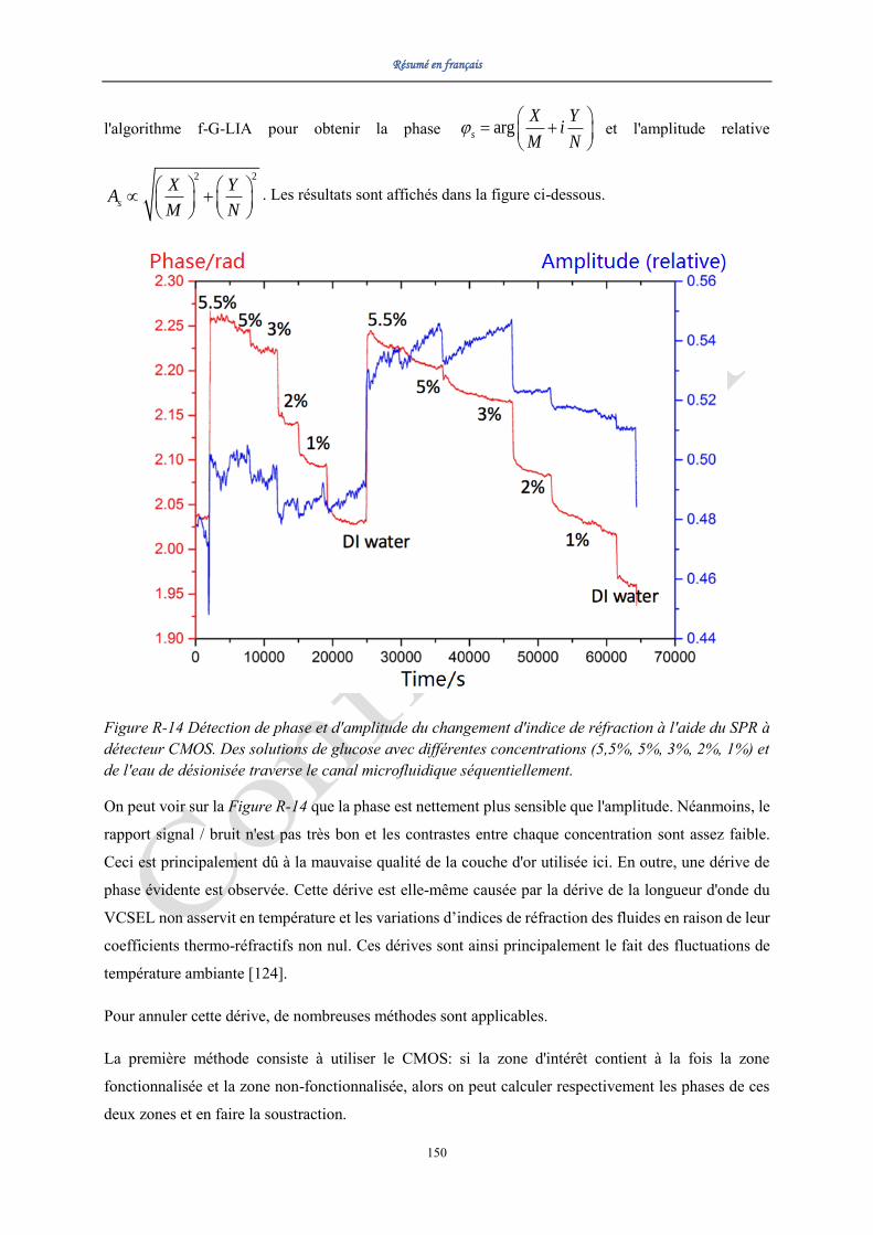
Résumé en français
150
l'algorithme f-G-LIA pour obtenir la phase args
X Yi
M N
= +
et l'amplitude relative
2 2
s
X YA
M N
+
. Les résultats sont affichés dans la figure ci-dessous.
Figure R-14 Détection de phase et d'amplitude du changement d'indice de réfraction à l'aide du SPR à
détecteur CMOS. Des solutions de glucose avec différentes concentrations (5,5%, 5%, 3%, 2%, 1%) et
de l'eau de désionisée traverse le canal microfluidique séquentiellement.
On peut voir sur la Figure R-14 que la phase est nettement plus sensible que l'amplitude. Néanmoins, le
rapport signal / bruit n'est pas très bon et les contrastes entre chaque concentration sont assez faible.
Ceci est principalement dû à la mauvaise qualité de la couche d'or utilisée ici. En outre, une dérive de
phase évidente est observée. Cette dérive est elle-même causée par la dérive de la longueur d'onde du
VCSEL non asservit en température et les variations d’indices de réfraction des fluides en raison de leur
coefficients thermo-réfractifs non nul. Ces dérives sont ainsi principalement le fait des fluctuations de
température ambiante [124].
Pour annuler cette dérive, de nombreuses méthodes sont applicables.
La première méthode consiste à utiliser le CMOS: si la zone d'intérêt contient à la fois la zone
fonctionnalisée et la zone non-fonctionnalisée, alors on peut calculer respectivement les phases de ces
deux zones et en faire la soustraction.

Résumé en français
151
La seconde méthode consiste à compenser uniquement la dérive de longueur d'onde du VCSEL: en
insérant un séparateur de faisceau entre YVO4 et le prisme de la Figure R-13, on peut mesurer la
différence de phase initiale entre la lumière p-polarisée et s-polarisée avant qu’elle ne soit réfléchie par
la couche d'or. Nous pouvons alors soustraire cette phase initiale de la phase mesurée en temps réel.
La Figure R-15 montre les résultats d'une expérience réalisée dans notre groupe sur un prototype plus
avancé (interrogation interférométrique et angulaire) pour démontrer l’efficacité de cette méthode. Dans
ce cas, une puce SPR commerciale est couplée sur un prisme à 45°, tandis que le procédé de modulation
de phase et le procédé de récupération de phase restent les mêmes.
Figure R-15 Capteur SPR à interrogation angulaire avec détection de phase et d'intensité. La
modulation de phase sinusoïdale est effectuée par modulation de longueur d'onde VCSEL. L'algorithme
f-G-LIA est utilisé pour extraire les informations de phase. Une puce SPR commerciale est utilisée sans
aucune microfluidique (dans l'air). (a) Réponse de phase au changement d'angle. (b) Réponse d'intensité
au changement d'angle.
Comme le montre la Figure R-15(b), à l'angle SPR (environ 44,3°), l'intensité est presque nulle, ce qui
implique que la qualité de cette puce SPR est excellente pour la mesure de phase. Sur la Figure R-15(a),
nous pouvons voir que la mesure de phase est très stable et qu'il y a une chute de phase quasi verticale
à l'angle SPR, ce qui prouve l'efficacité de notre méthode pour compenser la dérive de longueur d'onde
du VCSEL, ainsi que la faisabilité de notre méthode de détection de phase.
Nous pouvons utiliser la zone autour de l'angle SPR pour effectuer des détections de phase SPR très
sensibles, comme indiqué par la Figure R-15. Si nous fixons l'angle θk au centre de cette zone (angle
SPR), alors un minuscule changement d'indice de réfraction (e.g. 10-7) induit une différence de phase
notable. L’inconvénient est naturellement que l'intensité lumineuse du signal (lumière p-polarisée) est

Résumé en français
152
faible dans cette zone, tandis que l'intensité de référence (lumière s-polarisée) demeure forte que
d'habitude, ce qui n’est pas favorable à un rapport signal à bruit excellent. Il est clair que le rapport
signal à bruit déterminera ultimement la sensibilité de cette mesure de phase aux changements d’indices.
Nous pouvons proposer également une troisième méthode originale qui s'inspire de la technique de la
shearographie. Cette méthode à l’avantage de pouvoir fonctionné avec un signal entièrement p-polarisé,
comme représenté sur la figure ci-après:
Figure R-16 Combinaison d'interférométrie de type shearing et d'imagerie SPR.
On considère une puce fonctionnalisée par endroit (il faut au moins une zone de référence). Les
différentes parties du laser sont réfléchies par les différentes zones. Proche de θk, les différences de phase
peuvent être très grandes pour des différences d'intensité relativement plus faibles). Ainsi, à l’aide d’un
interféromètre de shearing comme celui représenté, nous pourrons observer l'intensité de la lumière
interférée aux zones de chevauchement, représentant la différence de phase entre les zones. En outre,
lorsque la température ambiante change, les changements de phase résultants sont presque les mêmes
pour différentes zones, de sorte que l'influence de la fluctuation de la température ambiante peut être
naturellement annulée.
En conclusion pour cette dernière partie plus exploratoire, nous avons étudié la possibilité d’utiliser
l’interférométrie à modulation de phase sinusoïdale dans un capteur SPR. Des expériences préliminaires
ont été conduites pour montrer l’applicabilité des méthodes de démodulation étudiées durant cette thèse.
Un capteur CMOS a été utilisé comme détecteur pour montrer la possibilité de faire de l'imagerie SPR
à l'avenir. Le problème de la phase initiale est résolu en utilisant LabVIEW pour contrôler l'ensemble
du système de mesure. En outre, plusieurs méthodes pour compenser l'influence de la fluctuation de la
température ambiante ont été décrites. Ces résultats ouvrent des perspectives pour le développement de
détecteurs SPR interférométriques précis, compacts, et robustes sans éléments couteux.
Résumé en français
153
Conclusions et perspectives
Dans le but d’élargir les possibilités de mesures interférométriques alliant simplicité, stabilité, fiabilité
et précision dans des systèmes simples (peu onéreux), nous avons étudié le signal interférométrique à
modulation de phase théoriquement et expérimentalement. La modulation de phase sinusoïdale a été
particulièrement considérée car elle est facile à réaliser et garantit une bonne précision sur la modulation
de phase, même à haute fréquence.
En particulier, cette modulation de phase sinusoïdale a été appliquée en holographie et en interférométrie
holographique. L'algorithme (f)-G-LIA a été utilisé pour récupérer les informations de phase, et les
résultats obtenus sont similaires à l'algorithme SPM traditionnel, pour des profondeurs de modulation
de phase favorables. En outre, des modulations de phase linéaires (en dents de scie) ou sinusoïdales ont
été mises en œuvre dans une configuration 2D-ESPI originale, permettant de réaliser des mesures
simultanées de champ de déplacement 2D. La modulation de phase sinusoïdale est également appliquée
à un capteur SPR sensible à la phase. Plusieurs méthodes pour compenser la fluctuation de la
température ambiante ont été proposées. La faisabilité de l’approche a été démontré expérimentalement.
Quelques perspectives peuvent être dressées : le problème de la phase initiale a été résolue
mathématiquement et expérimentalement, la plupart des expériences présentées dans cette thèse
n'intégrant pas de synchronisation. Cependant, afin d'améliorer la précision de la mesure et de faire des
mesures automatiques dans le futur, il sera nécessaire de contrôler la synchronisation entre la caméra et
les modulateurs, ou même de contrôler toute la procédure de mesure.
Pour un interféromètre à modulation de phase sinusoïdale classique, les données sont relativement
volumineuses et le traitement des données est relativement complexe, ce qui peut ralentir la vitesse de
mesure lorsqu'une caméra à haute fréquence d’acquisition ou un ordinateur à faible performance est
utilisé. La méthode du IBA (integrating bucket algorithm) peut être utilisée pour améliorer cette
situation.
En outre, nous pouvons nous inspirer des nouvelles "caméra LIA" qui intègre une détection synchrone
sur chaque pixel, et proposer de combiner la modulation de phase sinusoïdale avec le traitement du
signal analogique dans les "détecteurs intelligents". De cette manière, le temps d'acquisition des données
et de traitement des données peut être considérablement raccourci. La synchronisation entre la
modulation de phase et l'acquisition de données peut également être effectuée automatiquement.
Enfin, un enseignement général est qu’il demeurera important de choisir judicieusement le type de
modulateur, le type de modulation et l'algorithme de récupération de phase en fonction de la fréquence
de modulation, de la précision de modulation requise, des caractéristiques du bruit, de la longueur d'onde

Résumé en français
154
du laser et du coût souhaité. Ces différents facteurs doivent être considérés et bien équilibrés au sein des
prototypes à réaliser, en fonction de l’application ciblée.

Appendix
155
Appendix
Complete derivation processes of formulae
Eq. (0.30)
( )( ) ( )
( ) ( )
( ) ( )( ) ( )
( )
2 2
0 0
0
0 0
0
0 0 0
0
2
0
0
2 cos cos
2 cos cos
2 cos cos sin cos
2 cos cos
co
s n
s
i
T
r s r s s
T
r s s
T
r s s s
T
r s s
r s s
X A A A A t t dt
A A t t dt
A A t t t dt
A A t dt
TA A
= + + −
= −
=
=
=
+
Eq. (0.31)
( )( ) ( )
( ) ( )
( ) ( )( ) ( )
( )
2 2
0 0
0
0 0
0
0 0 0
0
2
0
0
2 cos sin
2 cos sin
2 cos c nsin
sin
s
os si sin
2 sin
in
T
r s r s s
T
r s s
T
r s s s
T
r s s
r s s
Y A A A A t t dt
A A t t dt
A A t t t dt
A A t dt
TA A
= + + −
= −
=
=
=
+

Appendix
156
Eq. (0.38)
( ) ( )
( )( )( ) ( )
( )( ) ( )
( )( ) ( )( )( ) ( )
( ) ( ) ( )
( ) ( )( )
0
2 2
0
0
0
0 2
1
2 1
1
2 cos sin cos 2
2 cos sin cos 2
2 cos sin cos sin sin sin cos 2
2 cos 2 cos
2
2 sin 2 1 sin
T
T
r s r s s
T
r s s
T
r s s s
n s
n
r s
n s
n
X I t C t dt
A A A A a t t dt
A A a t t dt
A A a t a t t dt
J a J a n t
A A
J a n t
+
=
+
−
=
=
= + + −
= −
= +
+
=
+ −
( )
( ) ( )
( )
0
2
2
0
2
cos 2
2 2cos cos 2
2 cos
T
T
r s s
r s s
t dt
A A J a t dt
TA A J a
=
=
Eq. (0.39)
( ) ( )
( )( )( ) ( )
( )( ) ( )
( )( ) ( )( )( ) ( )
( ) ( ) ( )
( ) ( )( )
0
2 2
0
0
0
0 2
1
2 1
1
2 cos sin sin
2 cos sin sin
2 cos sin cos sin sin sin sin
2 cos 2 cos
2
2 sin 2 1 sin
T
T
r s r s s
T
r s s
T
r s s s
n s
n
r s
n s
n
Y I t S t dt
A A A A a t t dt
A A a t t dt
A A a t a t t dt
J a J a n t
A A
J a n t
+
=
+
−
=
=
= + + −
= −
= +
+
=
+ −
( )
( ) ( )
( )
0
2
1
0
1
sin
2 2sin sin
2 sin
T
T
r s s
r s s
t dt
A A J a t dt
TA A J a
=
=

Appendix
157
Eq. (0.48)
( ) ( )
( )( )( ) ( )( )
( ) ( ) ( ) ( ) ( )( ) ( )( )
( ) ( ) ( )( ) ( )( )
( ) ( )
0
2 2
0
2 2
0 2
10 0
2 2
0
0
2 2
0
2 cos sin cos sin
2 cos 2 2 cos sin cos sin
2 cos sin cos sin
12 cos 2 sin
2
T
T
r s r s s
T T
r s n r s s
n
T
r s r s s
r s r s
X I t C t dt
A A A A a t a t dt
A A J a J a n t dt A A a t a t dt
T A A J a A A a t a t dt
T A A J a A A a
+
=
=
= + + −
= + + + −
= + + −
= + +
( )( ) ( )( )
( ) ( ) ( )( )
( ) ( ) ( )( ) ( )( )( )
( ) ( )
( ) ( ) ( )
0
2 2
0
0
2 2
0
0
2 2
0
0 2 2
1
cos
cos cos 2 sin
cos cos 2 sin cos sin 2 sin sin
cos
2 2 2 cos 2 cos 2
T
s s
T
r s r s s r s s
T
r s r s s r s s s
r s r s s
r s n s
n
t dt
T A A J a TA A A A a t dt
T A A J a TA A A A a t a t dt
T A A J a TA A
A A J a J a n t J
+
=
− + −
= + + −
= + + +
=
+
+
+ +
+ +
+
( ) ( )( )
( ) ( ) ( )
( ) ( ) ( )( )
1
10
2 2
0 0
0
2 2
0 0
2 sin 2 1 sin
cos 2 cos
2 cos1
T
n s
n
T
r s r s s r s s
r s r s s
a n t dt
T A A J a TA A A A J a dt
T A A J a TA A J a
+
−
=
−
= + +
= + +
+
+

Appendix
158
Eq. (0.50)
( ) ( )
( )( )( ) ( )( )
( ) ( ) ( )( ) ( )( ) ( )( )
( )( ) ( )( )
( )( ) ( )( )
0
2 2
0
2 2
2 1
10 0
0
0
2 cos sin sin sin
2 2 sin 2 1 2 cos sin sin sin
2 cos sin sin sin
12 sin 2 sin sin
2
T
T
r s r s s
T T
r s n r s s
n
T
r s s
T
r s s s
r
Y I t S t dt
A A A A a t a t dt
A A J a n t dt A A a t a t dt
A A a t a t dt
A A a t dt
TA A
+
−
=
=
= + + −
= + − + −
= −
= − − −
=
( )( )
( )( ) ( )( )( )
( ) ( )( ) ( ) ( ) ( )
0
0
2 1 0 2
1 10
sin 2 sin
cos sin 2 sin cos 2 sin sin
cos
2 2 sin 2 1 cos 2 2 2 cos 2 sin
cos
sin
cos
T
s s r s s
T
r s s r s s s
r s s
T
r s n s n s
n n
r s s r
A A a t dt
TA A A A a t a t dt
TA A
A A J a n t J a J a n t dt
TA A A A
+ +
−
= =
+
+ −
+ −
−
=
=
− +
+
=
( )( )
( )( )
0
0
0
2 si
si
n
21 n
T
s s
r s s
J a dt
TA A J a
= −
−

Appendix
159
Eq. (0.57)
( ) ( )
( )( ) ( )( ) ( )( )
( )( ) ( )( ) ( ) ( )( )
( )( ) ( )( )
( ) ( ) ( ) ( )
0
0
0
0
0 0
0
0 0 2
1
2 cos sin 2 cos cos sin
2 cos sin cos sin 2 cos cos sin
12 cos 2 sin cos
2
2 cos 2 cos 2
T
T
r s s r s s
T T
r s s r s s
T
r s s s
r s s n
n
X I t C t dt
A A a t A A J a a t dt
A A a t a t dt A A J a a t dt
A A a t dt
A A J a J a J a n t d
+
=
=
= − −
= − −
= − + −
− +
( )( ) ( )
( )( ) ( )( )( ) ( )
( )
( ) ( ) ( )
0
2
0
0
2
0
0
2
0
0 2
1
cos cos 2 sin 2 cos
cos cos 2 sin cos sin 2 sin sin 2 cos
2 cos cos
2 2 2 cos 2 cos 2
T
T
r s s r s s r s s
T
r s s r s s s r s s
r s s r s s
r s n s
n
t
TA A A A a t dt TA A J a
TA A A A a t a t dt TA A J a
TA A J a TA A
A A J a J a n t
+
=
+
+
= − −
= + −
= − +
+ +
+
( ) ( )( )
( ) ( )
( ) ( )( )
2 1
10
2
0 0
0
2
0 0
2 sin 2 1 sin
2 cos cos 2 co
21
s
2 cos
T
n s
n
T
r s s r s s r s s
r s s
J a n t dt
TA A J a TA A A A J a dt
TA A J a J a
+
−
=
−
+
+
= − +
= −
Appendix
160
Eq. (0.58)
( ) ( )
( )( ) ( )( ) ( )( )
( )( ) ( )( ) ( ) ( ) ( )( )
( )( ) ( )( )
( )( )
0
0
0
0 2 1
10 0
0
2 cos sin 2 cos sin sin
2 cos sin sin sin 2 cos 2 2 sin 2 1
2 cos sin sin sin
12 sin 2 sin si
2
T
T
r s s r s s
T T
r s s r s s n
n
T
r s s
r s s
Y I t S t dt
A A a t A A J a a t dt
A A a t a t dt A A J a J a n t dt
A A a t a t dt
A A a t
+
−
=
=
= − −
= − − −
= −
= − −
( )( )
( )( )
( )( ) ( )( )( )
( ) ( )( ) ( ) ( ) ( )
0
0
0
2 1 0 2
1 10
n
sin 2 sin
cos sin 2 sin cos 2 sin sin
cos
2 2 sin 2 1 cos
sin
c
2 2 2 cos 2 sin
os
T
s
T
r s s r s s
T
r s s r s s s
r s s
T
r s n s n s
n n
dt
TA A A A a t dt
TA A A A a t a t dt
TA A
A A J a n t J a J a n t dt
+ +
−
= =
−
= −
=
=
− +
+
+ −
+
=
−
( )( )
( )( )
0
0
0
cos 2 sin
21 sin
T
r s s r s s
r s s
TA A A A J a dt
TA A J a
−+
−=
Eq. (1.20)
( )( )( ) ( )( )
( )( ) ( )( )
( ) ( ) ( ) ( )( )
( ) ( ) ( ) ( )( ) ( ) ( )( )
2 2
0
0
0
0
0 2 0
10
2 0 0
' 2 cos sin cos 2
2 cos sin cos 2
2 2 cos 2 cos cos 2
2 2cos cos 2 cos 2 cos 2 sin 2 sin 2
T
r s r s s g
T
r s s g
T
r s n s g
n
r s s g g
X A A A A a t t t t dt
A A a t t t t dt
A A J a J a n t t t t dt
A A J a t t t t t t t
+
=
= + + + − +
= − + −
= + + −
= − − −
( ) ( )( )( )
0
2 0
2
2 cos 2 cos
2 cos 2 cos
T
r s g s
r s s
dt
TA A J a t t
TA A J a
= −
=

Appendix
161
Eq. (1.21)
( )( )( ) ( )( )
( )( ) ( )( )
( ) ( )( ) ( )( )
( ) ( ) ( ) ( )( ) ( ) ( )( )
2 2
0
0
0
0
2 1 0
10
1 0 0
0
' 2 cos sin sin
2 cos sin sin
2 2 sin 2 1 sin sin
2 2sin sin sin cos cos sin
T
r s r s s g
T
r s s g
T
r s n s g
n
T
r s s g g
Y A A A A a t t t t dt
A A a t t t t dt
A A J a n t t t t dt
A A J a t t t t t t t dt
+
−
=
= + + + − +
= − + −
= − + −
= − + −
( ) ( )( )( )
1 0
1
2 cos sin
2 cos sin
r s g s
r s s
TA A J a t t
TA A J a
= −
=

Appendix
162
Eq. (1.28)
( ) ( )
( )( )( ) ( )( )( )
( ) ( ) ( )
0
2 2
0
0
0 02 2
0
02 2
0 2
' ' '
2 cos sin cos sin
2 cos sin cos sin2 2
2 cos 22
T
T
r s r s s g
Tg g
r s r s s
g
r s n
X I t C t dt
A A A A a t t a t t dt
t t t tA A A A a t a t dt
t tA A J a J a n t
=
= + + + − +
− − = + + + − +
−= + + +
( ) ( )
10
0 0
0
0 0
2 2
0
2 cos sin cos sin2 2
cos sin sin2 2
cos
T
n
Tg g
r s s
g g
s
r s r s
dt
t t t tA A a t a t dt
t t t ta t a t
T A A J a A A
+
=
− − + + − +
− − + + + −
= + +
+
( ) ( )
( ) ( )
0 0 0
0 02 2
0
0
0
2 2
0
sin sin2 2
cos 2 cos sin cos 2 sin cos2 2
cos 2 cos2
T
g g
s
Tg g
r s r s s s
g
r s r s
dtt t t t
a t a t
t t t tT A A J a A A a t a t dt
t ta
T A A J a A A
− − + − + −
− − = + + − + −
−
= + +
( ) ( )
0
0 0 0
2 2
0
sin cos 2 cos sin sin2
cos 2 sin cos cos 2 sin cos sin2 2
cos 2 c
sin
si
os sin co
n
ss 2 cos sin si nn i2 2
g
s sT
g g
s s
s
r s r s
t tt a t
dtt t t t
a t a t
a t a t
T A A J a A A
−
− − +
+
+
+
= + +
0 cos 2 sin cos cos 2 sinsin cos sin2 2
sT
s s
dt
a t a t
+
+

Appendix
163
Eq. (1.29)
( ) ( )
( )( )( ) ( )( )( )
( ) ( ) ( )
0
2 2
0
0
0 02 2
0
02 2
2 1
' ' '
2 cos sin sin sin
2 cos sin sin sin2 2
2 sin 2 12
T
T
r s r s s g
Tg g
r s r s s
g
r s n
Y I t S t dt
A A A A a t t a t t dt
t t t tA A A A a t a t dt
t tA A J a n t
−
=
= + + + − +
− − = + + + − +
−= + − +
10
0 0
0
0 0
0
2 cos sin cos sin2 2
sin sin sin2 2
0
sin sin
T
n
Tg g
r s s
g g
s
r s
dt
t t t tA A a t a t dt
t t t ta t a t
A At
a t
+
=
− − + + − +
− − + + + −
= +
−− +
0 0
0 0
0
0 0
sin2 2
sin 2 cos sin sin 2 sin cos2 2
sin 2 cos sin cos 2 cos si2 2
cos
T
g g
s
Tg g
r s s s
g g
s
r s
dtt t t
a t
t t t tA A a t a t dt
t t t ta t a
A A
− − + −
− − = − − −
− −
=
−
0 0 0
n sin
sin 2 sin cos cos 2 sin cos sin2 2
sin 2 cos sin cos 2 cos sin sin2 2
sin 2 sin cos cos
cos
cos
2 sicos n cos2 2
sT
g g
s s
s s
r s
s
t
dtt t t t
a t a t
a t a t
A A
a t a t
− − −
=
− +
+
−
0 sin
T
s
dt

Appendix
164
Eq. (1.43)
( ) ( )( ) ( )
( )( ) ( )( )( ) ( )
( )( ) ( )( ) ( )
2 2
2 2
2 2
2
2 cos sin 1 sin
2 cos sin cos sin sin sin 1 sin
2 cos sin cos sin sin sin 1 sin2
2
r s r s s
r s r s s s
r sr s s s
r s
r s
r s
I t A A A A a t a t
A A A A a t a t a t
A AA A a t a t a t
A A
A A
A A
= + + + − + +
= + + + + + + +
+= + + + + + +
+
=
( )( )
( )( )
( )( )
( ) ( )( )
( ) ( )( )
( )( )
( ) ( ) ( )( )
2
2 2
0 2
1
1 sin2
cos cos sin
sin sin sin
cos sin cos sin
sin sin sin sin
1 sin2
cos 2 cos 2
2 sin 2
r s
s
s
s
s
r s
r s
s n
n
r s s
a tA A
a t
a t
a t a t
a t a t
A Aa t
A A
J a J a n t
A A J
+
=
+ +
+ + + + + + + + + +
++ +
+ + +
= +
( ) ( )( )( )
( ) ( ) ( ) ( )( )
( ) ( ) ( )( )( )
( ) ( )
2 1
1
0 2
1
2 1
1
2 2 2 2
0 0
sin 2 1
cos sin 2 cos 2
sin sin 2 sin 2 1
cos2 2
2
n
n
s n
n
s n
n
r s r ss
r s r s
r s
a n t
a t J a J a n t
a t J a n t
A A A AJ a J a
A A A A
A A
+
−
=
+
=
+
−
=
− +
+ + + +
+ + − +
+ ++ + +
=
( )
( ) ( )( )
( ) ( )( )( )
( ) ( )( ) ( )
( ) ( )( )( ) ( )
2
1
2 1
1
2
1
2 1
1
cos sin
cos 2 cos 2
sin 2 sin 2 1
cos 2 cos 2 sin
sin 2 sin 2 1 sin
s
s n
n
s n
n
s n
n
s n
n
a t
J a n t
J a n t
a J a n t t
a J a n t t
+
=
+
−
=
+
=
+
−
=
+
+ +
+ − +
+ + +
+ − + +

Appendix
165
( ) ( ) ( )
( ) ( )( )
( ) ( )( )( )
( ) ( )( )( ) ( )( )( )( )
( )
2 2 2 2
0 0
2
1
2 1
1
2
1
2 1
cos cos sin2 2
cos 2 cos 2
2 sin 2 sin 2 1
cos sin 2 1 sin 2 1
sin c
r s r ss s
r s r s
s n
n
r s s n
n
s n
n
s n
A A A AJ a J a a t
A A A A
J a n t
A A J a n t
a J a n t n t
a J a
+
=
+
−
=
+
=
−
+ ++ + + +
+ +
= + − +
+ + + − − +
+
( )( )( ) ( )( )( )
( ) ( ) ( )
( ) ( )( )
( ) ( )( )
1
2 2 2 2
0 0
2,4,...
1,3,...
os 2 2 cos 2
cos cos sin2 2
cos 2 cos
2 sin 2 sin
n
r s r ss s
r s r s
s m
m
r s s m
m
n t n t
A A A AJ a J a a t
A A A A
J a m t
A A J a m t
+
=
+
=
+
=
− + − +
+ ++ + + +
+ +
= + +
( ) ( )( ) ( ) ( )( )
( ) ( )( ) ( ) ( )( )
( )
1 1
3,5,... 1,3,...
1 1
0,2,... 2,4,...
2 2
0
cos sin sin
sin cos cos
cos2
2
s m m
m m
s m m
m m
r ss
r s
r s
a J a m t J a m t
a J a m t J a m t
A AJ a a
A A
A A
+ +
− +
= =
+ +
+ −
= =
+ + − +
+ + − +
++
=
+
( )
( ) ( )( ) ( ) ( )
( ) ( )( )
( ) ( )( )
( ) ( )( ) ( ) ( )( )
1
2 2
0 2 1
2,4,...
3,5,...
1 1
3,5,... 3,5,...
sin
cos 2sin sin2
cos 2 cos
sin 2 sin
cos sin sin
s
r ss s
r s
s m
m
s m
m
s m m
m m
J a
A Aa a J a J a J a t
A A
J a m t
J a m t
a J a m t J a m t
+
=
+
=
+ +
− +
= =
++ + − + +
+ +
+ +
+ + − +
( ) ( )( ) ( ) ( )( )1 1
2,4,... 2,4,...
sin cos coss m m
m m
a J a m t J a m t + +
+ −
= =
+ + − +

Appendix
166
( ) ( )
( ) ( ) ( )( ) ( )
( ) ( ) ( )( )( ) ( )( )
( ) ( ) ( )( )( ) ( )( )
2 2
0 1
2 2
1 0 2
1 1
2,4,...
1 1
3,5,...
cos sin2
2 sin cos sin2
2
2 cos sin cos
2 sin cos sin
r ss s
r s
r ss s
r sr s
m s m m s
m
m s m m s
m
A AJ a aJ a
A A
A Aa J a J a J a t
A AA A
J a a J a J a m t
J a a J a J a m t
+
+ −
=
+
− +
=
++
++ + + − + =
+ − +
+ − +
+
+
+
( ) ( )( ) ( )( )
( )
( )
1
2,4,... 3,5,...
0,2,...
1 3, ..
0
, .
2 sin cos sin
cos sin
2
cos si
sin cos c n
n
os si
r s m
m m
m
r s
m
m
m
m
A A R t m t R m t
m t
R R
R m t
A A
R m m t
m
m t
m
m
+ +
= =
+
=
+
=
+
= + + + + +
−
= + +
Eq. (1.48)
( ) ( )
( ) ( ) ( ) ( )( ) ( )
( ) ( )
( )
( ) ( ) ( ) ( )( )( )
0
2
0
2
0
1 1
2
2
2 cos 2 sin 2 cos 2
2 cos 2 cos 2
cos 2
cos 2 2 cos si
cos 2 s
n
in 2
T
T
r s
T
r s
r s
r s m s m m s
X I t C t dt
A A t t t dt
A
R
RA t dt
TA A
TA A J a a J a J a
R
+ −+
=
= −
=
=
= −
Eq. (1.49)
( ) ( )
( ) ( )( ) ( )
( )
( ) ( ) ( )( )
0
1
0
2
1
0
1
2 2
1 0 2
2 sin cos cos sin sin
2 cos sin
cos
cos 2 sin cos2
T
T
r s
T
r s
r s
r sr s s s
r s
Y I t S t dt
A A R t t t dt
A A R t dt
TA A R
A ATA A a J a a J a J a
A A
=
= +
=
=
+ =
+ −
+

Appendix
167
Eq. (1.61)
( ) ( )
( ) ( ) ( ) ( )( ) ( )
( ) ( )
( )
( ) ( ) ( ) ( )( )( )
0
3
0
2
1
0
1
3 2 4
2 sin 3 cos 3 cos 3 sin 3 sin 3
2 cos 3 sin 3
cos 3
cos 3 2 sin cos
T
T
r s
T
r s
r s
r s s s
Y I t S t dt
A A R t t t dt
A A R t dt
TA A R
TA A J a a J a J a
=
= +
=
−+
=
=
Eq. (1.76)
( ) ( )
( )( ) ( )
( ) ( )( )( )
( )( )
( ) ( )
( )( ) ( )
0
2 2
2 2
0 0 1
2 2
2 cos sin 1 sin
cos sin2 cos sin
2
2 cos sin
sin
2 cos sin sin
2
T
r s r s sT
r sr s s s
r s
r s s
r s
r s s
X I t C t dt
A A A A a t a t
a t dtA AA A J a aJ a
A A
A A a t
A A a t
A A a t a t
A
=
+ + + − + +
+
= +− +
+ −
+ + +=
+ + − +
−
( ) ( )( )
( )( )0
0 1
cos sin
cos sin
T
r s s s
a t dt
A J a aJ a
+
According to Eq. (1.34), we can get the first term:
( )( ) ( )( )1
0
0 0
2 cos sin cos sin
2 sin 2 cos cos2 2
T
r s s
r s s
T A A a t a t dt
TA A J a J a
= + −
= +
According to the trigonometric identities and the symmetry properties of periodic functions, we know
that:
( )( ) ( )( ) ( ) ( )( ) ( )0 0 0
sin sin sin sin cos cos sin sin 0
T T T
a t t dt a t t dt a t t dt = =
According to the definition of Bessel function:

Appendix
168
( )( ) ( )( ) ( ) ( ) ( )2
1 1
0 0
2 1 2cos sin cos sin
2
T
a t t dt t a t d t J a TJ a
= = =
So with the help of the trigonometric identities, we can get the second term:
( ) ( ) ( )( )
( ) ( ) ( )( ) ( ) ( )( )
( )( )( ) ( )( )( )
( )( ) ( )( )( )
( )
2 2
2
0
2 2
0 0
02 2
0
2 2
sin cos sin
sin cos cos sin cos sin cos sin
cossin sin sin sin
2
sincos sin cos sin
2
T
r s
T T
r s
T
r s T
r s
T A A a t a t dt
A A a t a t dt t a t dt
t a t t a t dt
A A a
t a t t a t dt
A A
= + +
= + +
+ + −
= + + + + −
= +
( ) ( )( )1 1
sin0
2
0
a T J a J a
+ − +
=
The third term can be deduced as follow:

Appendix
169
( )( ) ( ) ( )( )
( )( ) ( )( ) ( ) ( )( )
( )
3
0
0
2 cos sin sin cos sin
sin2 cos sin sin cos sin sin
2
sin cos 2 sin cos cos 2 cos sin2 2 2 2
T
r s s
T
r s s s
r s s s
T A A a t a t a t dt
tA A a a t a t a t a t dt
A A a t a t a t
= + − +
+ = + − + + −
= + + − + + −
+
−
( )
( )
0
0
sin cos 2 cos sin2 2
sin cos 2 sin cos2 2
sin 2 cos sin sin 2 cos sin2 2 2 21
2s
T
sT
r s
s
s s
r s
dt
t a t
A A a dt
t a t
t a t t a t
A A a
+ + −
= + + + −
+ + + − + + − + +
=
+
0in 2 sin cos sin 2 sin cos
2 2 2 2
sin 2 cos sin2 2 2 2
sin 2 cos sin2 2 2 21
2
T
s s
s
s
r s
dt
t a t t a t
t a t
t a t
A A a
+ + + − + + − + +
+ + + −
+ + − + +
=
−
−
0sin 2 sin cos
2 2 2 2
sin 2 sin cos2 2 2 2
T
s
s
dt
t a t
t a t
+ + + + −
+ + − + + −
−
where
0
0
0 0
1
sin 2 cos sin2 2 2 2
sin 2 cos sin2 2
sin 2 cos sin cos cos 2 cos sin sin2 2 2 2
0 sin2
T
s
T
s
T T
s s
s
t a t dt
t a t dt
t a t dt t a t dt
TJ
+ + + −
= + −
= + − + + −
−
−
− −
+
= − −
1
2 cos2
sin 2 cos2 2
s
a
T J a
=
+

Appendix
170
0
0
0 0
1
sin 2 cos sin2 2 2 2
sin 2 cos sin2 2
sin 2 cos sin cos cos 2 cos sin sin2 2 2 2
0 sin 2 c2
T
s
T
s
T T
s s
s
t a t dt
t a t dt
t a t dt t a t dt
TJ a
−
−
− −
+ − + +
= − +
= − + −
= + −
1
os2
sin 2 cos2 2
sT J a
−
=
0
0
0
0
sin 2 sin cos2 2 2 2
sin 2 sin cos2 2
sin 2 sin sin2 2 2
sin 2 sin sin2 2 2 2 2
sin 2
T
s
T
s
T
s
T
s
t a t dt
t a t dt
t a t dt
t a t dt
t a
+ + + −
= + −
= + − −
= − − − − +
−
−
−
−
= −
0
0 0
1
1
sin sin2 2 2
sin 2 sin sin cos cos 2 sin sin sin2 2 2 2 2 2
0 cos 2 sin2 2
cos 2 sin2 2
T
s
T T
s s
s
s
t dt
t a t dt t a t dt
TJ a
T J a
− +
= − − + + − − +
= +
=
−
− −
+
+

Appendix
171
0
0
0
0
sin 2 sin cos2 2 2 2
sin 2 sin cos2 2
sin 2 sin sin2 2 2
sin 2 sin sin2 2 2 2 2
sin 2
T
s
T
s
T
s
T
s
t a t dt
t a t dt
t a t dt
t a t dt
t a
+ − + +
= − +
= − − +
= − + − + +
−
−
−
−
= +
0
0 0
1
1
sin sin2 2 2
sin 2 sin sin cos cos 2 sin sin sin2 2 2 2 2 2
0 cos 2 sin2 2
cos 2 sin2 2
T
s
T T
s s
s
s
t dt
t a t dt t a t dt
TJ a
T J a
+ +
= + + + + +
= + − −
−
−
= −
−
+
−
So we can get:
1 1
3
1 1
1
sin 2 cos sin 2 cos2 2 2 21
2cos 2 sin cos 2 sin
2 2 2 2
sin 2 cos sin2 2 2
2
s s
r s
s s
s s
r s
T J a T J a
T A A a
T J a T J a
J a JT
A A a
+
= + −
+
+ −
+
+ −
−
=
1
1 1
1
1
1 1
2 cos2
cos 2 sin cos 2 sin2 2 2 2
2sin 2 cos2 2
22s
cos
sin
cos s
in 2 sin2 2
2 cos 2 si2 2
i2
n
s s
s
r s
s
r s
a
J a J a
J aT
A A a
J a
TA A a J a J a
+ −
=
+
= +
+
−
n sin2
s
According to Jacobi-Anger expansion and the orthogonality of trigonometric functions, the forth term
can be deduced:
Appendix
172
( ) ( )( ) ( )( )
( ) ( )( ) ( )( )
( ) ( )( ) ( ) ( ) ( )
( ) ( ) ( )( )
4 0 1
0
0 1
0
0 1 0 2
10
2
0 0 1
2 cos sin cos sin
2 cos sin cos sin
2 cos sin 2 cos 2
2 cos sin
T
r s s s
T
r s s s
T
r s s s n
n
r s s s
T A A J a aJ a a t dt
A A J a aJ a a t dt
A A J a aJ a J a J a n t dt
TA A J a aJ a J a
=
= −
= −
= − +
+
= −
+
+
+
So we get X:
( ) ( ) ( )( )
( )
1 2 3 4
0 0
1 1
2
0 0 1
2
0 0 0
2 sin 2 cos cos2 2
2 cos 2 sin sin2 2 2 2
2 cos s
0
in
2 sin 2 cos 22 2
cos sin
r s s
r s s
r s s s
r s
X T T T T
TA A J a J a
TA A a J a J a
TA A J a aJ a J a
TA A J a J a J a
= + + +
= +
+ +
−
+ −
+
+
=
( ) ( )1 1 0 1cos si
cos
2 cos 2 sin 2 sin2 2 2 2
n
s
r s sTA A a J a J a J a J a
+ −
+
Eq. (1.77)
( ) ( )
( )( ) ( )
( ) ( )( )( )
( )( )
( ) ( )
( )( ) ( )
0
2 2
2 2
0 0 1
2 2
2 cos sin 1 sin
sin2 cos sin
2
2 cos sin
sin
2 cos si
sin
n sin
2
T
r s r s sT
r sr s s s
r s
r s s
r s
r s s
Y I t S t dt
A A A A a t a t
a t dtA AA A J a aJ a
A A
A A a t
A A a t
A A a t a t
A
=
+ + + − + +
+
= +− +
+ −
+ + +=
+ + − +
−
( ) ( )( )
( )( )0
0 1
sin
cos sin
sin
T
r s s s
a t dt
A J a aJ a
+
According to Eq. (1.35), we can get the first term:

Appendix
173
( )( ) ( )( )1
0
0 0
2 cos sin sin sin
2 sin 2 cos sin2 2
T
r s s
r s s
T A A a t a t dt
TA A J a J a
= + −
= −
According to the trigonometric identities and the symmetry properties of periodic functions, we know
that:
( )( ) ( )( ) ( ) ( )( ) ( )0 0 0
sin sin sin sin cos cos sin sin 0
T T T
a t t dt a t t dt a t t dt = =
According to the definition of Bessel function:
( )( ) ( )( ) ( ) ( ) ( )2
1 1
0 0
2 1 2cos sin cos sin
2
T
a t t dt t a t d t J a TJ a
= = =
So with the help of the trigonometric identities, we can get the second term:
( ) ( ) ( )( )
( ) ( ) ( )( ) ( ) ( )( )
( )( )( ) ( )( )( )
( )( ) ( )( )( )
( )
2 2
2
0
2 2
0 0
02 2
0
2 2
sin sin sin
sin cos sin sin cos sin sin sin
coscos sin cos sin
2
sinsin sin sin sin
2
T
r s
T T
r s
T
r s T
r s
T A A a t a t dt
A A a t a t dt t a t dt
t a t t a t dt
A A a
t a t t a t dt
A A
= + +
= + +
− − +
= + + + − −
= +
( ) ( )( )
( ) ( )
1 1
2 2
1
cos0
2
cosr s
a T J a J a
T A A a J a
+ +
= +
The third term can be deduced as follow:

Appendix
174
( )( ) ( ) ( )( )
( )( ) ( )( ) ( ) ( )( )
( )
3
0
0
2 cos sin sin sin sin
sin2 sin sin sin sin sin sin
2
sin sin 2 sin cos sin 2 cos sin2 2 2 2
T
r s s
T
r s s s
r s s s
T A A a t a t a t dt
tA A a a t a t a t a t dt
A A a t a t a t
= + − +
+ = + − − + −
= + + − − + −
+
−
( )
( )
0
0
sin sin 2 cos sin2 2
sin sin 2 sin cos2 2
cos 2 cos sin cos 2 cos sin2 2 2 21
2c
T
sT
r s
s
s s
r s
dt
t a t
A A a dt
t a t
t a t t a t
A A a
+ + −
= − + + −
+ − + + − + + + −
=
+
0os 2 sin cos cos 2 sin cos
2 2 2 2
cos 2 cos sin2 2 2 2
cos 2 cos sin2 2 2 21
2
T
s s
s
s
r s
dt
t a t t a t
t a t
t a t
A A a
+ − + + − + + + −
+ − + +
− + + + −
=
−
−
0cos 2 sin cos
2 2 2 2
cos 2 sin cos2 2 2 2
T
s
s
dt
t a t
t a t
+ + − + +
− + + + − −
−
Where
0
0
0 0
1
cos 2 cos sin2 2 2 2
cos 2 cos sin2 2
cos 2 cos sin cos sin 2 cos sin sin2 2 2 2
cos 2 cos2
T
s
T
s
T T
s s
s
t a t dt
t a t dt
t a t dt t a t dt
TJ a
−
−
−
+ − + +
= − +
= − − −
=
−
−
1
02
cos 2 cos2 2
sT J a
−
−
=

Appendix
175
0
0
0 0
cos 2 cos sin2 2 2 2
cos 2 cos sin2 2
cos 2 cos sin cos sin 2 cos sin sin2 2 2 2
cos2
T
s
T
s
T T
s s
s
t a t dt
t a t dt
t a t dt t a t dt
T
− + + + −
= − + −
= − + − + + −
−
−
= − −+
−
−
1
1
2 cos 02
cos 2 cos2 2
s
J a
T J a
+
=
+
0
0
0
0
cos 2 sin cos2 2 2 2
cos 2 sin cos2 2
cos 2 sin sin2 2 2
cos 2 sin sin2 2 2 2 2
cos 2
T
s
T
s
T
s
T
s
t a t dt
t a t dt
t a t dt
t a t dt
t a
+ − + +
= − +
= − − +
= − + − + +
−
−
−
−
= +
0
0 0
1
1
sin sin2 2 2
cos 2 sin sin cos sin 2 sin sin sin2 2 2 2 2 2
sin 2 sin 02 2
sin 2 sin2 2
T
s
T T
s s
s
s
t dt
t a t dt t a t dt
TJ a
T J a
+ +
= + + − + +
= − − −
=
− −
−
+
−

Appendix
176
0
0
0
0
cos 2 sin cos2 2 2 2
cos 2 sin cos2 2
cos 2 sin sin2 2 2
cos 2 sin sin2 2 2 2 2
cos
T
s
T
s
T
s
T
s
t a t dt
t a t dt
t a t dt
t a t dt
− + + + −
= − + −
= − + − −
= − − − − − +
−
−
−
−
−
=
0
0 0
1
1
2 sin sin2 2 2
cos 2 sin sin cos sin 2 sin sin sin2 2 2 2 2 2
sin 2 sin 02 2
sin 2 sin2 2
T
s
T T
s s
s
s
t a t dt
t a t dt t a t dt
TJ a
T J a
− − +
= − − − + + − − +
= − +
=
−
− −
+
+−
So we get:
1 1
3
1 1
1 1
cos 2 cos cos 2 cos2 2 2 21
2sin 2 sin sin 2 sin
2 2 2 2
cos 2 cos cos2 2 2
2
s s
r s
s s
s s
r s
T J a T J a
T A A a
T J a T J a
J a JT
A A a
+
=
−
+
− +
−
=
+
− +
1 1
1
1
1 1
c
2 cos2
sin 2 sin si
os
sin
co
n 2 sin2 2 2 2
2co
s sin
s 2 cos2 2
22cos 2 sin
2 2
2 cos 2 sin2 2 2
s s
s
r s
s
r s
a
J a J a
J aT
A A a
J a
TA A a J a J a
+ −
=
−
= −
− +
cos
2s
According to Jacobi-Anger expansion and the orthogonality of trigonometric functions, the forth term
can be deduced:

Appendix
177
( ) ( )( ) ( )( )
( ) ( )( ) ( )( )
( ) ( )( ) ( ) ( )( )
4 0 1
0
0 1
0
0 1 2 1
10
2 cos sin sin
2 cos sin sin sin
2
sin
cos sin 2 cos 2 1
0
T
r s s s
T
r s s s
T
r s s s n
n
T A A J a aJ a a t dt
A A J a aJ a a t dt
A A J a aJ a J a n t dt
−
=
= −
= −
= −
+
=
+
+ −
So we get Y:
( ) ( )
1 2 3 4
2 2
0 0 1
1 1
2 sin 2 cos sin cos2 2
2 cocos sins 2 sin cos2 2 2 2
r s s r s
r s s
Y T T T T
TA A J a J a T A A a J a
TA A a J a J a
= + + +
= − +
+ −
+
Eq. (1.96)
( )
( ) ( )
( ) ( )
21
0
2
00,2,... 1,3,...
2
02,4,... 1
0
,3,...
0
2 cos sin sin cos cos sin
2 sin sin cos cos s
cos si
2
n
ii ns n
r s m
m m
r s m
m
m
r
m
m
s
U I t dt
A A m t m t R m m t m m t dt
A A m t R m m t m m t dt
A
R m m
R R m
RA
+ +
= =
+ +
= =
=
= − + +
= − + +
+
=
( ) ( )1
2 2
2,4,... 1,3,...
s1 1 1 1
sin cosin2
m
m
m
m
m m
m R m mm m m
R
+
+ +
= =
− − − − + +
−
Eq. (1.97)
( )
( ) ( )
( ) ( )
2
2
0,2,... 1,3,...2
2,4,... 1,3,...2
0
2 cos sin sin cos cos sin
2 sin sin cos
cos sin
sin cos sin
2
r s m
m m
r s m
m m
m
r
m
U I t dt
A A m t m t R m m t m m t dt
A A m t R m m t m m t dt
R m
R
A
m
A
m
R
+ +
= =
+ +
= =
=
= − + +
= − + +
=
+
( ) ( )1
2 2
2,4,... 1,3,...
0
1 1 1 1sins co
2in s
m m
s m
m m
mR m R m mm m m
R
+
+ +
= =
− − − + +
−

Appendix
178
Eq. (1.98)
( )
( ) ( )
( ) ( )
3
23
3
2
0,2,... 1,3,...
3
2
2,4,... 1
0
,3,...
2 cos sin sincos sin
si
cos cos sin
2 sin sin cos cos s
2
n in
r m
m
s m
m m
r s m
m m
U I t dt
A A m t m t R m m t m m t dt
A A m t R m m t m m t d
R
t
m m
R R m
+ +
= =
+ +
= =
=
= − + +
= −+ + +
=
( ) ( )1
2 2
2,4,... 1 3 . .
0
, , .
1 1 1 1sin co
2sin s
m m
r s m
m
m
m
A A m R m mm m m
R R
+
+ +
= =
− − − − + +
−
Eq. (1.99)
( )
( ) ( )
( ) ( )
2
34
2
2
3
0,2,... 1,3,...2
2
3
2,4,... 1,3,..
0
.2
2 cos sin sin cos cos sin
2 sin sin cos cos sin
cos sin
sin
r s m
m m
r s mm
m m
m
U I t dt
A A m t m t R m m t m m t dt
A A m t R m m t m m t d
R m m
R R m t
+ +
= =
+ +
= =
=
= − + +
= − ++ +
( ) ( )1
2 2
2,4,... 1,3,..
0
.
1 1 1 12 sin cos n si
2
m m
r s m
m m
mRA A m R m mm m m
R
+
+ +
= =
− − − − − = +− +
Eq. (1.109)
( )
( ) ( ) ( )( )
( ) ( ) ( )( )( )( )
( )( )
( )
1
21 2 3 4
1 2
1,3,...
2 2
1 0 2
1
2
1 1
3,5,...
12 2
2
1
14 4 sin
2
4sin2 sin cos
2
14 2 sin cos sin
2 sin 18 sin
m
m
mr s
r ss s
r s
m
m s m m s
m
m
r s
m
mr s
U U U UP L R m
A A m
A AJ a J a J a
A A
J a J a J a mm
A AJ a m
A A m
+
+
=
+
+
− +
=
+
=
−− + + −= = − =
+−= + + −
−+ −
+ −= +
+
−
( ) ( )( )( )
,3,...
1
2
1 1
1,3,...
sin
14 sin cos
s
m
m m s
m
J a J a mm
+
+
+
− +
=
− −
+

Appendix
179
Eq. (1.110)
( )
( ) ( ) ( )( )( )( )
( )( )
( ) ( )( )( )
21 2 3 4
2 1
2,4,...
2
1 1
2,4,...
2 2
1 1
2,4,... 2,4,...
si1 1
4 42
1 14 2 cos sin
1 1 1 18 co
n
sin
sin sins 4
m
mr s
m
m s m m s
m
m m
m s m m
m
m
m
U U U UP L m
A A m
J a J a J a mm
J a m J a J a mm m
R
+
=
+
+ −
=
+ +
+ −
= =
+
− −− + − += = =
− −= −
− − − − =
+ −
sin s
Angular spectrum method
When the complex light field on the plane of z=z0 is known to be ( )0
,zE x y , then we can use 2D Fourier
transform to decompose it into plane waves along different directions described by different wave
vectors ( ), ,x y zk k k k= :
( ) ( )( )2 2 2
0
0 0
ˆ , ,x y x yi k x k y k k k z
z x y zE k k E x y e dxd y− + + − −
=
where 2
k k
= = , 2 2 2
z x yk k k k= − − .
Then the complex light field on the plane of z=z1 can be calculated by the inverse Fourier transform:
( ) ( ) ( ) ( )2 2 22 2 201 0
1 0
ˆ, ,x y x yx y
i k x k y k k k zi k k k z z
z z x y x yE x y E k k e e dk dk+ + − −− − − =

References
181
References
1 Young, T. (1804). Experimental demonstration of the general law of the interference of
light. Philosophical Transactions of the Royal society of London, 94(1804), 1.
2 Scheider, W. (1986). Do the" Double Slit" experiment the way it was originally done. The Physics
Teacher, 24, 217-219.
3 Basdevant, J. L. (2009). Le Mémoire de Fresnel sur la diffraction de la lumière. Bibnum. Textes
fondateurs de la science.
4 Michelson, A. A. (1881). The relative motion of the Earth and of the luminiferous ether. American
Journal of Science, (128), 120-129.
5 Michelson, A. A., & Morley, E. W. (1887). On the Relative Motion of the Earth and of the
Luminiferous Ether. Sidereal Messenger, vol. 6, pp. 306-310, 6, 306-310.
6 Zehnder, L. (1891). Ein neuer interferenzrefraktor. Springer.
7 Mach, L. (1892). Ueber einen interferenzrefraktor. Zeitschrift für Instrumentenkunde, 12(3), 89.
8 Hadjar, Y., Cohadon, P. F., Aminoff, C. G., Pinard, M., & Heidmann, A. (1999). High-sensitivity
optical measurement of mechanical Brownian motion. EPL (Europhysics Letters), 47(5), 545.
9 Libbrecht, K. G., & Black, E. D. (2014). A Laser Interferometer for the Undergraduate Teaching
Laboratory Demonstrating Picometer Sesitivity. arXiv preprint arXiv:1407.0075.
10 Creath, K. (1988). V phase-measurement interferometry techniques. In Progress in optics (Vol. 26,
pp. 349-393). Elsevier.
11 Reid, G. T. (1986). Automatic fringe pattern analysis: a review. Optics and Lasers in
Engineering, 7(1), 37-68.

References
182
12 Moore, D. T., Murray, R., & Neves, F. B. (1978). Large aperture ac interferometer for optical
testing. Applied optics, 17(24), 3959-3963.
13 Basile, G., Bergamin, A., Cavagnero, G., & Mana, G. (1991). Phase modulation in high-resolution
optical interferometry. Metrologia, 28(6), 455.
14 Sasaki, O., & Okazaki, H. (1986). Sinusoidal phase modulating interferometry for surface profile
measurement. Applied optics, 25(18), 3137-3140.
15 Kato, J. I., Yamaguchi, I., & Ping, Q. (1993). Automatic deformation analysis by a TV speckle
interferometer using a laser diode. Applied optics, 32(1), 77-83.
16 Furstenau, N., Schmidt, M., Horack, H., Goetze, W., & Schmidt, W. (1997). Extrinsic Fabry-Perot
interferometer vibration and acoustic sensor systems for airport ground traffic monitoring. IEE
Proceedings-Optoelectronics, 144(3), 134-144.
17 Steinchen, W., & Yang, L. (2003). Digital shearography: theory and application of digital speckle
pattern shearing interferometry (Vol. 93). Bellingham: SPIE press.
18 Lin, V. S. Y., Motesharei, K., Dancil, K. P. S., Sailor, M. J., & Ghadiri, M. R. (1997). A porous
silicon-based optical interferometric biosensor. Science, 278(5339), 840-843.
19 Fan, X., White, I. M., Shopova, S. I., Zhu, H., Suter, J. D., & Sun, Y. (2008). Sensitive optical
biosensors for unlabeled targets: A review. analytica chimica acta, 620(1-2), 8-26.
20 Duval, D., González-Guerrero, A. B., Dante, S., Osmond, J., Monge, R., Fernández, L. J., ... &
Lechuga, L. M. (2012). Nanophotonic lab-on-a-chip platforms including novel bimodal
interferometers, microfluidics and grating couplers. Lab on a Chip, 12(11), 1987-1994.
21 Micó, V., Garcia-Monreal, J., & Zalevsky, Z. (2009). Quantitative phase imaging by common-path
interferometric microscopy: application to super-resolved imaging and nanophotonics. Journal of
Nanophotonics, 3(1), 031780.
22 Al Mohtar, A., Vaillant, J., Sedaghat, Z., Kazan, M., Joly, L., Stoeffler, C., ... & Bruyant, A. (2014).
Generalized lock-in detection for interferometry: application to phase sensitive spectroscopy and near-
field nanoscopy. Optics express, 22(18), 22232-22245.
23 Zheng, J. (2004). Analysis of optical frequency-modulated continuous-wave interference. Applied
optics, 43(21), 4189-4198.
24 Sasaki, O., & Okazaki, H. (1986). Analysis of measurement accuracy in sinusoidal phase
modulating interferometry. Applied optics, 25(18), 3152-3158.

References
183
25 Tatsuno, K., & Tsunoda, Y. (1987). Diode laser direct modulation heterodyne
interferometer. Applied optics, 26(1), 37-40.
26 Sasaki, O., Okazaki, H., & Sakai, M. (1987). Sinusoidal phase modulating interferometer using the
integrating-bucket method. Applied optics, 26(6), 1089-1093.
27 Dante, S., Duval, D., Sepúlveda, B., González-Guerrero, A. B., Sendra, J. R., & Lechuga, L. M.
(2012). All-optical phase modulation for integrated interferometric biosensors. Optics express, 20(7),
7195-7205.
28 Zhu, Y., Vaillant, J., François, M., Montay, G., & Bruyant, A. (2017). Co-axis digital holography
based on sinusoidal phase modulation using generalized lock-in detection. Applied optics, 56(13),
F97-F104.
29 Schnars, U., & Jueptner, W. (2005). Digital Holography: Digital hologram recording,
reconstruction principle, and related techniques. Springer.
30 Kreis, T. (2006). Handbook of holographic interferometry: optical and digital methods. John Wiley
& Sons.
31 Jones, R., & Wykes, C. (1989). Holographic and speckle interferometry (Vol. 6). Cambridge
university press.
32 Huang, Y. H., Ho, H. P., Wu, S. Y., & Kong, S. K. (2012). Detecting phase shifts in surface
plasmon resonance: a review. Advances in Optical Technologies, 2012.
33 Yamaguchi, I., & Zhang, T. (1997). Phase-shifting digital holography. Optics letters, 22(16), 1268-
1270.
34 Vandenrijt, J. F., & Georges, M. P. (2010). Electronic speckle pattern interferometry and digital
holographic interferometry with microbolometer arrays at 10.6 μm. Applied optics, 49(27), 5067-5075.
35 Creath, K. (1985). Phase-shifting speckle interferometry. Applied Optics, 24(18), 3053-3058.
36 Lokberg, O. J., & Hogmoen, K. (1976). Use of modulated reference wave in electronic speckle
pattern interferometry. Journal of Physics E: Scientific Instruments, 9(10), 847.
37 Gabor, D. (1949). Microscopy by reconstructed wave-fronts. Proc. R. Soc. Lond. A, 197(1051),
454-487.
38 Gabor, D. (1951). Microscopy by reconstructed wave fronts: II. Proceedings of the Physical
Society. Section B, 64(6), 449.

References
184
39 Mueller, R. K., & Sheridon, N. K. (1966). Sound holograms and optical reconstruction. Applied
Physics Letters, 9(9), 328-329.
40 Schnars, U., & Jüptner, W. (1994). Direct recording of holograms by a CCD target and numerical
reconstruction. Applied optics, 33(2), 179-181.
41 Schnars, U., & Jüptner, W. P. (2002). Digital recording and numerical reconstruction of
holograms. Measurement science and technology, 13(9), R85.
42 Fienup, J. R. (1982). Phase retrieval algorithms: a comparison. Applied optics, 21(15), 2758-2769.
43 Fienup, J. R. (2013). Phase retrieval algorithms: a personal tour. Applied optics, 52(1), 45-56.
44 Yamaguchi, I., Kato, J. I., & Ohta, S. (2001). Surface shape measurement by phase-shifting digital
holography. Optical review, 8(2), 85-89.
45 Heflinger, L. O., Wuerker, R. F., & Brooks, R. E. (1966). Holographic interferometry. Journal of
Applied Physics, 37(2), 642-649.
46 Kreis, T. (1986). Digital holographic interference-phase measurement using the Fourier-transform
method. JOSA A, 3(6), 847-855.
47 Bruyant, A., Vaillant, J., Wu, T. H., Zhu, Y., Huang, Y., & Al Mohtar, A. (2017). Interferometry
Using Generalized Lock-in Amplifier (G-LIA): A Versatile Approach for Phase-Sensitive Sensing and
Imaging. In Optical Interferometry. InTech.
48 Bruyant, A. P., Vaillant, J., & Al Mohtar, A. (2016). U.S. Patent No. 9,518,869. Washington, DC:
U.S. Patent and Trademark Office.
49 Zhu, Y., Vaillant, J., Montay, G., & Bruyant, A. (2016, July). Generalized lock-in detection applied
to lens-less digital holographic interferometry. In Digital Holography and Three-Dimensional
Imaging (pp. DTh3C-3). Optical Society of America.
50 František, Š., Matúš, K., & Martin, O. (2013). The Verification of Fixture for Shear Load with
Optical Method ESPI. Am. J. Mech. Eng, 1(7), 180-184.
51 Robinson, D. W., & Williams, D. C. (1986). Digital phase stepping speckle interferometry. Optics
communications, 57(1), 26-30.
52 Holo3, “Speckle interferometry,” http://www.holo3.com/en/experiment-simulation/speckle-
interferometry/ .

References
185
53 Yang, L., Xie, X., Zhu, L., Wu, S., & Wang, Y. (2014). Review of electronic speckle pattern
interferometry (ESPI) for three dimensional displacement measurement. Chinese Journal of
Mechanical Engineering, 27(1), 1-13.
54 Yang, L. X., & Ettemeyer, A. (2003). Strain measurement by three-dimensional electronic speckle
pattern interferometry: potentials, limitations, and applications. Optical Engineering, 42(5), 1257-
1267.
55 DantecDynamics, “3D ESPI System (Q-300),” https://www.dantecdynamics.com/3d-espi-system-q-
300 .
56 Homola, J., Yee, S. S., & Gauglitz, G. (1999). Surface plasmon resonance sensors. Sensors and
Actuators B: Chemical, 54(1-2), 3-15.
57 Wijaya, E., Lenaerts, C., Maricot, S., Hastanin, J., Habraken, S., Vilcot, J. P., ... & Szunerits, S.
(2011). Surface plasmon resonance-based biosensors: From the development of different SPR
structures to novel surface functionalization strategies. Current Opinion in Solid State and Materials
Science, 15(5), 208-224.
58 Wong, C. L., & Olivo, M. (2014). Surface plasmon resonance imaging sensors: a
review. Plasmonics, 9(4), 809-824.
59 Goodrich, T. T., Lee, H. J., & Corn, R. M. (2004). Direct detection of genomic DNA by
enzymatically amplified SPR imaging measurements of RNA microarrays. Journal of the American
Chemical Society, 126(13), 4086-4087.
60 Cooper, M. A. (2002). Optical biosensors in drug discovery. Nature reviews Drug discovery, 1(7),
515.
61 Tao, N. J., Boussaad, S., Huang, W. L., Arechabaleta, R. A., & D’Agnese, J. (1999). High
resolution surface plasmon resonance spectroscopy. Review of Scientific Instruments, 70(12), 4656-
4660.
62 Jorgenson, R. C., & Yee, S. S. (1993). A fiber-optic chemical sensor based on surface plasmon
resonance. Sensors and Actuators B: Chemical, 12(3), 213-220.
63 Li, Y. C., Chang, Y. F., Su, L. C., & Chou, C. (2008). Differential-phase surface plasmon resonance
biosensor. Analytical Chemistry, 80(14), 5590-5595.
64 Kabashin, A. V., Patskovsky, S., & Grigorenko, A. N. (2009). Phase and amplitude sensitivities in
surface plasmon resonance bio and chemical sensing. Optics Express, 17(23), 21191-21204.

References
186
65 Kashif, M., Bakar, A. A. A., Arsad, N., & Shaari, S. (2014). Development of phase detection
schemes based on surface plasmon resonance using interferometry. Sensors, 14(9), 15914-15938.
66 Su, Y. D., Chen, S. J., & Yeh, T. L. (2005). Common-path phase-shift interferometry surface
plasmon resonance imaging system. Optics letters, 30(12), 1488-1490.
67 Zeng, S., Yu, X., Law, W. C., Zhang, Y., Hu, R., Dinh, X. Q., ... & Yong, K. T. (2013). Size
dependence of Au NP-enhanced surface plasmon resonance based on differential phase
measurement. Sensors and Actuators B: Chemical, 176, 1128-1133.
68 He, P., Kang, Z. Y., Wan, X. Q., & Fang, H. X. (2016). Research on protein thermal condensation
detection based on phase modulation SPR imaging. Biotechnology and applied biochemistry, 63(1),
138-144.
69 Chang-Hasnain, C. J. (2000). Tunable vcsel. IEEE Journal of Selected Topics in Quantum
Electronics, 6(6), 978-987.
70 Mateus, C. F., Huang, M. C., Li, P., Cunningham, B. T., & Chang-Hasnain, C. J. (2004). Compact
label-free biosensor using VCSEL-based measurement system. IEEE Photonics Technology
Letters, 16(7), 1712-1714.
71 Yoshino, T., Nara, M., Mnatzakanian, S., Lee, B. S., & Strand, T. C. (1987). Laser diode feedback
interferometer for stabilization and displacement measurements. Applied optics, 26(5), 892-897.
72 Sasaki, O., Takahashi, K., & Suzuki, T. (1990). Sinusoidal phase modulating laser diode
interferometer with feedback control system to eliminate external disturbance. Optical
Engineering, 29(12), 1511-1516.
73 Li, Z., Wang, X., Bu, P., Huang, B., & Zheng, D. (2009). Sinusoidal phase-modulating laser diode
interferometer insensitive to the intensity modulation of the light source. Optik-International Journal
for Light and Electron Optics, 120(16), 799-803.
74 Wang, B., Wang, X., Li, Z., & Sasaki, O. (2012). Sinusoidal phase-modulating laser diode
interferometer insensitive to intensity modulation for real-time displacement measurement with
feedback control system. Optics Communications, 285(18), 3827-3831.
75 Wang, X., Wang, X., Qian, F., Chen, G., Chen, G., & Fang, Z. (1999). Photothermal modulation of
laser diode wavelength: application to sinusoidal phase-modulating interferometer for displacement
measurements. Optics & Laser Technology, 31(8), 559-564.
76 Dimitrova, T. L., & Weis, A. (2008). The wave-particle duality of light: A demonstration
experiment. American Journal of Physics, 76(2), 137-142.

References
187
77 Dudley, D. G. (1994). Mathematical foundations for electromagnetic theory. New York: IEEE
press.
78 Wikipedia, “Wave interference,” https://en.wikipedia.org/wiki/Wave_interference .
79 Wikipedia, “Interferometry,” https://en.wikipedia.org/wiki/Interferometry .
80 He, G., & Wang, X. (2009). Real-time micro-vibration measurement in sinusoidal phase-
modulating interferometry. Optik-International Journal for Light and Electron Optics, 120(3), 101-
105.
81 Dubois, A. (2001). Phase-map measurements by interferometry with sinusoidal phase modulation
and four integrating buckets. JOSA A, 18(8), 1972-1979.
82 Massie, N. A., Nelson, R. D., & Holly, S. (1979). High-performance real-time heterodyne
interferometry. Applied Optics, 18(11), 1797-1803.
83 Howard, J. (1992). Multiorder rotating grating interferometer. Applied optics, 31(10), 1419-1425.
84 Kothiyal, M. P., & Delisle, C. (1984). Optical frequency shifter for heterodyne interferometry using
counterrotating wave plates. Optics letters, 9(8), 319-321.
85 Wyant, J. C. (1975). Use of an ac heterodyne lateral shear interferometer with real–time wavefront
correction systems. Applied optics, 14(11), 2622-2626.
86 Wyant, J. C., Koliopoulos, C. L., Bhushan, B., & George, O. E. (1984). An optical profilometer for
surface characterization of magnetic media. ASLE transactions, 27(2), 101-113.
87 Dubois, A. (2017). A simplified algorithm for digital fringe analysis in two-wave interferometry
with sinusoidal phase modulation. Optics Communications, 391, 128-134.
88 Stetson, K. A. (2009). Mathematical refocusing of images in electronic holography. Applied
optics, 48(19), 3565-3569.
89 Wikipedia, “Angular spectrum method,” https://en.wikipedia.org/wiki/Angular_spectrum_method .
90 ThorLabs, “Resolution Test Targets,”
https://www.thorlabs.com/newgrouppage9.cfm?objectgroup_id=4338 .
91 Mann, C. J., Yu, L., Lo, C. M., & Kim, M. K. (2005). High-resolution quantitative phase-contrast
microscopy by digital holography. Optics Express, 13(22), 8693-8698.
92 Micó, V., Zalevsky, Z., Ferreira, C., & García, J. (2008). Superresolution digital holographic
microscopy for three-dimensional samples. Optics express, 16(23), 19260-19270.

References
188
93 Sobieranski, A. C., Inci, F., Tekin, H. C., Yuksekkaya, M., Comunello, E., Cobra, D., ... & Demirci,
U. (2015). Portable lensless wide-field microscopy imaging platform based on digital inline
holography and multi-frame pixel super-resolution. Light: Science & Applications, 4(10), e346.
94 Tahara, T., Quan, X., Otani, R., Takaki, Y., & Matoba, O. (2018). Digital holography and its
multidimensional imaging applications: a review. Microscopy, 67(2), 55-67.
95 Aebischer, H. A., & Waldner, S. (1999). A simple and effective method for filtering speckle-
interferometric phase fringe patterns. Optics Communications, 162(4-6), 205-210.
96 Wikipedia, “Kernel (image processing),” https://en.wikipedia.org/wiki/Kernel_(image_processing) .
97 Wikipedia, “Digital holographic microscopy,”
https://en.wikipedia.org/wiki/Digital_holographic_microscopy#cite_ref-Kemper2_3-0 .
98 Kemper, B., Langehanenberg, P., & Von Bally, G. (2007). Digital Holographic Microscopy: A
New Method for Surface Analysis and Marker‐Free Dynamic Life Cell Imaging. Optik &
Photonik, 2(2), 41-44.
99 Zhang, J., Di, J., Li, Y., Xi, T., & Zhao, J. (2015). Dynamical measurement of refractive index
distribution using digital holographic interferometry based on total internal reflection. Optics
express, 23(21), 27328-27334.
100 He, M. G., Zhang, S., Zhang, Y., & Peng, S. G. (2015). Development of measuring diffusion
coefficients by digital holographic interferometry in transparent liquid mixtures. Optics express, 23(9),
10884-10899.
101 Pérez-Huerta, J. S., Saucedo-Anaya, T., Moreno, I., Ariza-Flores, D., & Saucedo-Orozco, B.
(2017). Digital holographic interferometry applied to the investigation of ignition process. Optics
express, 25(12), 13190-13198.
102 Li, J., Li, S., Sun, Y., & An, H. (2001, April). Dynamic speckle pattern technique on measuring in-
plane deformation of metal surface. In 24th International Congress on High-Speed Photography and
Photonics (Vol. 4183, pp. 309-313). International Society for Optics and Photonics.
103 Moore, A. J., & Tyrer, J. R. (1990). An electronic speckle pattern interferometer for complete in-
plane displacement measurement. Measurement science and technology, 1(10), 1024.
104 Xie, X., Yang, L., Chen, X., Xu, N., & Wang, Y. (2013, October). Review and comparison of
temporal-and spatial-phase shift speckle pattern interferometry for 3D deformation measurement.
In Sixth International Symposium on Precision Mechanical Measurements (Vol. 8916, p. 89160D).
International Society for Optics and Photonics.

References
189
105 ThorLabs, “Piezoelectric Actuators with Attached Strain Gauges,”
https://www.thorlabs.com/newgrouppage9.cfm?objectgroup_id=10975 .
106 Goldstein, R. M., Zebker, H. A., & Werner, C. L. (1988). Satellite radar interferometry: Two-
dimensional phase unwrapping. Radio science, 23(4), 713-720.
107 Ghiglia, D. C., & Pritt, M. D. (1998). Two-dimensional phase unwrapping: theory, algorithms, and
software (Vol. 4). New York: Wiley.
108 Wikipedia, “Surface plasmon resonance,”
https://en.wikipedia.org/wiki/Surface_plasmon_resonance .
109 Liedberg, B., Nylander, C., & Lundström, I. (1995). Biosensing with surface plasmon resonance—
how it all started. Biosensors and Bioelectronics, 10(8), i-ix.
110 Lofas, S. (1995). Dextran modified self-assembled monolayer surfaces for use in biointeraction
analysis with surface plasmon resonance. Pure and applied chemistry, 67(5), 829-834.
111 Löfås, S., & Johnsson, B. (1990). A novel hydrogel matrix on gold surfaces in surface plasmon
resonance sensors for fast and efficient covalent immobilization of ligands. Journal of the Chemical
Society, Chemical Communications, (21), 1526-1528.
112 Tetz, K. A., Pang, L., & Fainman, Y. (2006). High-resolution surface plasmon resonance sensor
based on linewidth-optimized nanohole array transmittance. Optics letters, 31(10), 1528-1530.
113 Chinowsky, T. M., Quinn, J. G., Bartholomew, D. U., Kaiser, R., & Elkind, J. L. (2003).
Performance of the Spreeta 2000 integrated surface plasmon resonance affinity sensor. Sensors and
Actuators B: Chemical, 91(1-3), 266-274.
114 Soelberg, S. D., Chinowsky, T., Geiss, G., Spinelli, C. B., Stevens, R., Near, S., ... & Furlong, C.
E. (2005). A portable surface plasmon resonance sensor system for real-time monitoring of small to
large analytes. Journal of industrial microbiology and biotechnology, 32(11-12), 669-674.
115 Wikipedia, “Spreeta,” https://en.wikipedia.org/wiki/Spreeta .
116 GE Healthcare Life Science, “Biacore 8K,” https://www.gelifesciences.com/en/bs/shop/protein-
analysis/spr-label-free-analysis/systems/biacore-8k-p-05540 .
117 “In-Vitro Diagnostics & POC – LamdaGen corporation” http://lamdagen.com/applications/in-
vitro-diagnostics-poc/ .
118 Haes, A. J., & Van Duyne, R. P. (2004). A unified view of propagating and localized surface
plasmon resonance biosensors. Analytical and bioanalytical chemistry, 379(7-8), 920-930.

References
190
119 Bhagawati, M., You, C., & Piehler, J. (2013). Quantitative real-time imaging of protein–protein
interactions by LSPR detection with micropatterned gold nanoparticles. Analytical chemistry, 85(20),
9564-9571.
120 Raphael, M. P., Christodoulides, J. A., Delehanty, J. B., Long, J. P., Pehrsson, P. E., & Byers, J.
M. (2013). Quantitative LSPR imaging for biosensing with single nanostructure
resolution. Biophysical journal, 104(1), 30-36.
121 Ruemmele, J. A., Hall, W. P., Ruvuna, L. K., & Van Duyne, R. P. (2013). A localized surface
plasmon resonance imaging instrument for multiplexed biosensing. Analytical chemistry, 85(9), 4560-
4566.
122 Raether, H. (1988). Surface Plasmons on Smooth and Rough Surfaces and on Gratings. Springer-
Verlag, Berlin.
123 Zeng, S., Hu, S., Xia, J., Anderson, T., Dinh, X. Q., Meng, X. M., ... & Yong, K. T. (2015).
Graphene–MoS2 hybrid nanostructures enhanced surface plasmon resonance biosensors. Sensors and
Actuators B: Chemical, 207, 801-810.
124 Vaillant, J., & Bruyant, A. (2017). An unbalanced interferometer insensitive to wavelength
drift. Sensors and Actuators A: Physical, 268, 188-192.
125 heliotis AG, “heliCamTM C3 - Fast Lock-In Camera,” http://heliotis.ch/html/lockInCameraC3.htm .
126 heliotis AG, “High-speed Lock-IN CMOS camera with pixel-level signal processing,”
https://www.swissphotonics.net/libraries.files/Heliotis_presentation.pdf .
127 Liu, Y., Shen, Y., Ma, C., Shi, J., & Wang, L. V. (2016). Lock-in camera based heterodyne
holography for ultrasound-modulated optical tomography inside dynamic scattering media. Applied
physics letters, 108(23), 231106.
128 Liu, Y., Ma, C., Shen, Y., & Wang, L. V. (2016). Bit-efficient, sub-millisecond wavefront
measurement using a lock-in camera for time-reversal based optical focusing inside scattering
media. Optics letters, 41(7), 1321-1324.

Exploration de méthodes de détection interférométriques à modulation de phase continue Dans cette thèse, nous nous intéressons aux si-gnaux interférométriques à modulation de phase continue, dans le but de développer des dispositifs de détection performants et originaux pour des applications en mécanique et en optique. Nous présentons d'abord plusieurs des techniques de modulation et démodulation employées dans ce contexte. Nous nous focalisons sur les modulations de phase sinusoïdales (SPM), qui sont particulière-ment avantageuses pour les dispositifs de modula-tion les plus largement accessibles. Nous proposons alors des solutions au problème de synchronisation ainsi qu'au problème éventuel de modulation d'amplitude concomitante à la modulation SPM. Ces techniques de démodulations sont ensuite ap-pliquées à 3 dispositifs expérimentaux développés au cours de cette thèse. Il s'agit d'abord d'un dispo-sitif d'holographie digitale compact sans lentille, mettant en œuvre une modulation SPM simple, pour l'imagerie et la mesure de déplacement. Nous utili-sons ensuite une technique de modulation à double fréquence pour réaliser des mesures bidimension-nelles de champ de déformation, à l'aide d'un dispo-sitif ESPI (interférométrie de speckle) original. Cette approche permet une mesure simultanée dans les 2 directions du plan à l'aide d'un seul système de laser et caméra. Finalement, nous présentons un instrument de type SPR (Surface Plasmon Re-sonance) compact mettant en œuvre une détection interférométrique SPM par modulation de longueur d'onde, dans lequel la modulation d'amplitude est prise en compte avec succès. Mots clés : interférométrie – modulation de phase – interférométrie holographique – interférométrie par granularité – résonance plasmonique de surface.
Yunlong ZHU Doctorat : Matériaux, Mécanique, Optique, Nanotechnologie
Année 2018
Exploration of Interferometric Detection Methods based on Continuous Phase Modulation In this thesis, interference signals with continuous phase modulations are theoretically and experimen-tally analyzed in order to develop cost-efficient solutions for sensing application in mechanics and optics. Several common phase modulation functions and phase retrieval algorithms are presented. We mainly focus on sinusoidal phase modulation (SPM), which is especially attractive for the most accessible mod-ulators (e.g. electro-optical or piezoelectrical modu-lators). In such case, the demodulation process must handle synchronization issue as well as a possible intensity modulation induced by the SPM. Mathematical solutions are proposed in this context. These demodulation techniques are then applied to three experimental devices developed during this thesis. First of all, a lens-less co-axis digital holog-raphy setup has been built, and SPM has been ap-plied for imaging and displacement measurement. Then we use a dual-frequency modulation technique to perform two-dimensional deformation field meas-urements using an original ESPI (Electronic Speckle Pattern Interferometry) device. This approach allows for simultaneous measurement of the displacement along two different axes using a single laser and a single camera. Finally, we present a compact SPR (Surface Plasmon Resonance) instrument imple-menting SPM interferometric detection through wavelength modulation, where the amplitude modu-lation is successfully taken into account. Keywords: interferometry – phase modulation – holographic interferometry – speckle metrology – surface plasmon resonance.
Ecole Doctorale "Sciences pour l’Ingénieur"
Thèse réalisée en partenariat entre :
Copyright © 2022 FDOKUMEN