ENHANCED STATISTICAL STABILITY IN COHERENT INTERFEROMETRIC

IMAGING

LILIANA BORCEA∗, JOSSELIN GARNIER† , GEORGE PAPANICOLAOU† , AND CHRYSOULA TSOGKA§

Abstract. We analyze the resolution and statistical fluctuations of images when the ambient medium is random andscattering can be modeled primarily by wavefront distortion. We compare the coherent interferometric imaging method to thewidely used Kirchhoff migration and show how the latter loses statistical stability at an exponential rate with the distance ofpropagation. In Kirchhoff migration we form images by superposing the array data back propagated to the image domain. Incoherent interferometry we back propagate local cross correlations of the array data. This is a denoising process that enhancesthe signal-to-noise ratio of images but also reduces the resolution. We quantify analytically the trade-off between enhancedstability and reduced resolution in coherent interferometric imaging.

Key words. array imaging, coherent interferometric imaging, data denoising, image resolution.

1. Introduction. We study the mathematical problem of imaging remote sources or reflectors in het-

erogeneous (cluttered) media with passive and active arrays of sensors. Because the inhomogeneities in the

medium are not known, and they cannot be estimated in detail from the data gathered at the array, we

model the uncertainty about the clutter with spatial random perturbations of the wave speed. The goal is

to carry out analytically a comparative study of the resolution and signal-to-noise ratio (SNR) of two array

imaging methods: the widely used Kirchhoff migration (KM) and coherent interferometry (CINT). By noise

in the images we mean fluctuations that are due to the random medium.

Kirchhoff migration [5, 6] and its variants are widely used in seismic inversion, radar [14] and elsewhere.

It forms images by superposing the wave fields received at the array, delayed by the travel times from

the array sensors to the imaging points. KM works well in smooth and known media, where there is no

wave scattering and the travel times can be estimated accurately. It also works well with data that has

additive, uncorrelated measurement noise, provided the array is large, because the noise is averaged out

by the summation over the many sensors, as expected from the law of large numbers. This is illustrated

for example in [12], where it is also shown how KM fails to image in heterogeneous (cluttered) media. KM

images in such media are unreliable and difficult to interpret because of the significant wave distortion by the

inhomogeneities. The distortion is very different from additive, uncorrelated noise, and it cannot be reduced

by simply summing over the sensors in the array. CINT images efficiently in clutter [8, 9, 10], at ranges

that do not exceed one or two transport mean free paths [20]. Beyond such ranges the problem becomes

much more difficult, specially in the case of active arrays, because the clutter backscatter overwhelms the

echoes from the reflectors that we wish to image. Coherent imaging in such media may work only after

pre-processing the data with filters of clutter backscatter, as is done in [12, 2]. The clutter considered in

this paper is not as strong as in [12, 2], so imaging with CINT alone, without any extra array data filtering,

gives good results.

The CINT method has been introduced in [8, 9, 10] for mitigating wave distortion effects induced by

clutter. It forms images by superposing time delayed, local cross-correlations of the wave fields received at

∗Computational and Applied Mathematics, Rice University, Houston, TX 77005. (borcea@caam.rice.edu)†Laboratoire de Probabilites et Modeles Aleatoires & Laboratoire Jacques-Louis Lions, Universite Paris VII, Site Chevaleret,

75205 Paris Cedex 13, France. (garnier@math.jussieu.fr)‡Mathematics, Stanford University, Stanford, CA 94305. (papanicolaou@stanford.edu)§Applied Mathematics, University of Crete and IACM/FORTH, GR-71409 Heraklion, Greece. (tsogka@tem.uoc.gr)

1

the array. Here local cross correlations means that they are computed in appropriate time windows and

over limited array sensor offsets. It has been shown with analysis and verified with numerical simulations

[8, 9, 10, 11, 7] that the time and offset thresholding in the computation of the cross-correlations is essential

in CINT, because it introduces a smoothing that is necessary to achieve statistical stability, at the expense

of some loss in resolution. By statistical stability we mean negligibly small fluctuations in the CINT image

even when cumulative fluctuation effects in the random medium are not small.

The statistical stability of CINT has been studied analytically in [9, 11] using the paraxial wave approx-

imation that neglects back scattering in random media. However, a detailed comparative study between KM

and CINT has not been carried out because the scattering model in [9, 11] is too complicated to allow an

analysis of the SNR.

In this paper we consider the resolution versus statistical stability trade-off in CINT using a relatively

simple random travel time model for the effects of the random medium. We compute the mean and SNR∗

of the KM and CINT point spread functions, and show explicitly that no matter how large the array is,

KM loses statistical stability at an exponential rate with the distance of propagation, the range. CINT is

superior to KM because its SNR does not decay with range and it can be improved by increasing the array

aperture.

The random travel time model [21, 19] captures wavefront distortions in heterogeneous media, but not the

delay spread (coda) due to multiple scattering. The model is valid in the geometrical optics regime in random

media with weak fluctuations and large correlation lengths compared to the wavelength [21, 19, 23, 15]. It

ignores diffraction and amplitude fluctuations that cause scintillation, and it is widely used in adaptive optics

for approximating wavefront distortions due to propagation in turbulent media [22, 16]. We use it in this

paper because it allows us to carry out analytically a comparative study of resolution and statistical stability

of CINT and KM.

The paper is organized as follows: We begin in section 2 with the statement of the array imaging problem

and the mathematical expression of the KM and CINT imaging functions for passive and active arrays. The

random travel time model is considered in section 3 with details of its derivation provided for completeness

in Appendix A. We study the point spread function in passive array imaging in section 4. The resolution

and stability analysis of KM is in section 4.3 and that of CINT in section 4.4. In section 5 we study active

array imaging. We illustrate the analytical results with numerical simulations in section 6. We end with a

summary in section 7.

2. Formulation of the array imaging problem. To image sources or reflectors in a medium we

record the wave fields at a remote array of sensors. By an array we mean a collection of N sensors that

are placed sufficiently close together to behave as a continuum aperture, the array. The basic propagation

model is the scalar (acoustic) wave equation in n+1 dimensions, where n = 1, 2, and the array data consists

of measurements of the acoustic pressure p. We refer to the measurements as time traces to emphasize that

they are functions of time t.

2.1. Imaging with passive arrays. In the source localization problem the sensors are receivers and

the array is called passive. The excitation comes from the unknown source and the receivers at ~xr, for

r = 1, . . . , N , record the traces p(t, ~xr). Since we study the point spread function, we assume a point source

∗The SNR is defined as the mean value of the imaging function at its peak, divided by its standard deviation.

2

Array of sensors

~y⋆

f(t)

~xr

Fig. 2.1. Setup for source localization with a passive array.

at location ~y, as illustrated in Figure 2.1. It emits a pulse

f(t) = e−iωotfB(t), (2.1)

with Fourier transform

f(ω) =

∫ ∞

−∞

dt f(t)eiωt = fB(ω − ωo). (2.2)

Here ωo is the central frequency, fB is the baseband pulse, and B denotes the bandwidth, that is, the size of

the frequency interval that supports fB. We take for convenience a Gaussian shaped pulse fB(t) = e−B2t2/2,

so that we can evaluate explicitly the integrals that arise in the analysis and obtain explicit relations for the

resolution and the SNR of CINT and KM. We have

f(t) = e−iωot−B2t2

2 , f(ω) =

√2π

Be−

(ω−ωo)2

2B2 , (2.3)

and we assume that the width of f(t), which scales as 1/B, is much smaller than the travel time of the waves

from the source to the array.

The inverse problem is to determine the location ~y of the source from the array data traces, modeled

by the convolution of the pulse with the Green’s function G(t, ~xr, ~y) of the wave equation

p(t, ~xr) = f(t) ⋆ G(t, ~xr, ~y) =

∫ ∞

−∞

dω

2πf(ω)G(ω, ~xr, ~y)e−iωt. (2.4)

We analyze it using two imaging methods: KM and CINT. The KM imaging function is [5, 6]

IKM(~yS) =

N∑

r=1

p(τo(~xr, ~yS), ~xr) =

N∑

r=1

∫ ∞

−∞

dω

2πp(ω, ~xr)e

−iωτo(~xr,~yS), (2.5)

where τo(~xr, ~yS) is the travel time from the point ~yS at which we image to the receiver at ~xr in the

background medium without fluctuations. In this paper we assume a homogeneous background medium and

3

so τo(~xr, ~yS) = |~xr − ~yS |/co. In general τo is given by Fermat’s principle. The KM function gives an image

by superposing the time traces back propagated to ~yS with travel time delays.

The CINT imaging function [8, 9] is

ICINT(~yS) =

N∑

r,r′=1

∫ ∞

−∞

dω

2π

∫ ∞

−∞

dω′

2πΦ

(ω − ω′

Ωd

)Ψ

(~xr − ~xr′

Xd

)

×p(ω, ~xr)p(ω′, ~xr′)e−iωτo(~xr,~yS)+iω′τo(~xr′ ,~yS), (2.6)

where the bar denotes complex conjugate and Φ and Ψ are windows with support scaled by two parameters

Ωd and Xd. We use these windows to threshold the frequency and sensor offsets over which we form cross-

correlations of the array traces. In general, ICINT does not have a simple expression in the time domain, like

IKM, because the sensor offset threshold Xd may vary in the bandwidth [9]. If Xd were a constant, we could

write

ICINT(~yS) =

N∑

r,r′=1

Ψ

(~xr − ~xr′

Xd

)∫ ∞

−∞

dt ΩdΦ (tΩd) p(τo(~xr, ~y

S) − t, ~xr

)p (τo(~xr′ , ~yS) − t, ~xr′).

This is somewhat similar to (2.5), but it forms the image by superposing the back propagated cross-

correlations of the array traces over receivers that are not further than Xd apart and in a time interval

scaled by 1/Ωd. It is only when Xd is as large as the array aperture, and Ωd → ∞, that the imaging methods

become essentially the same, with ICINT(~yS) proportional to∣∣IKM(~yS)

∣∣2.The thresholding by Xd and Ωd in the CINT imaging function (2.6) is essential when imaging in clutter.

It introduces a smoothing in the imaging process that leads to statistically stable results, as shown in [11, 9]

and with more analytical detail in this paper. The optimal thresholding is determined by the trade-off

between the smoothing for stability and loss of resolution. The optimal parameters Xd and Ωd are related

to the decoherence length and frequency that describe how the wave fields lose coherence due to scattering

in clutter. They may be determined directly from the data using statistical signal processing tools such as

the variogram [17, 18], but the estimation may not be accurate enough. It is better to determine Xd and Ωd

adaptively during the image formation, as explained in [9].

2.2. Imaging with active arrays. The setup for imaging a reflector with an active array of sensors

is illustrated in Figure 2.2. The reflector is centered at ~y and the array is active, because its sensors play

the dual role of sources and receivers. We denote the source locations by ~xs and the receivers by ~xr. Even

though s and r are indices that take integer values between 1 and N , we use them consistently in the paper

to remind us which are the sources and receivers. We assume for simplicity that all the sources emit the

same pulse f(t) given by (2.3), and we denote the time traces recorded at the receivers by p(t, ~xr, ~xs).

The imaging problem is to determine the support of the reflector from the array data traces. We study it

using KM and CINT, and since we are interested in the point spread function, we assume that the reflector

is a point at ~y with reflectivity one. Then the model of the time traces is

p(t, ~xr, ~xs) = f(t) ⋆ G(t, ~xr, ~y) ⋆ G(t, ~xs, ~y) =

∫ ∞

−∞

dω

2πf(ω)G(ω, ~xr, ~y)G(ω, ~xs, ~y)e−iωt. (2.7)

4

Array of sensors

~y

~xs

~xr

D

Fig. 2.2. Setup for imaging with an active array.

The KM imaging function with active arrays is

IKM(~yS) =

N∑

r,s=1

p(τo(~xr, ~yS) + τo(~xs, ~y

S), ~xr, ~xs)

=

N∑

r,s=1

∫ ∞

−∞

dω

2πp(ω, ~xr, ~xs)e

−iω[τo(~xr,~yS)+τo(~xs,~yS)]. (2.8)

It is similar to (2.5) except that we sum over both the sources and receivers, and we account for the additional

travel time between the source and the point ~yS at which we form the image.

The CINT imaging function is

ICINT(~yS) =N∑

s,s′=1

N∑

r,r′=1

∫ ∞

−∞

dω

2π

∫ ∞

−∞

dω′

2πΦ

(ω − ω′

Ωd

)Ψ

(~xr − ~xr′

Xd

)Ψ

(~xs − ~xs′

Xd

)

×p(ω, ~xr, ~xs)p(ω′, ~xr′ , ~xs′)e−iω[τo(~xr ,~yS)+τo(~xs,~yS)]+iω′[τo(~xr′ ,~yS)+τo(~xs′ ,~y

S)]. (2.9)

It forms the image with the superposition of the back propagated cross-correlations of the traces at sources

and receivers that are not further than Xd apart.

2.3. Simplifying assumptions on the geometry, the array and the thresholding windows.

We assume for simplicity that the array is in the plane xn+1 = 0 in Rn+1, where n = 1 or 2. The center of

the array is the origin of the system of coordinates, with axis xn+1 in the range direction, from the array to

the point source or reflector that we wish to locate. The sensor locations are

~xr = (xr, 0), xr ∈ A ⊂ Rn, r = 1, . . .N, (2.10)

and the unknown source or reflector location is

~y = (y = 0, L). (2.11)

5

Here L is the range and y ∈ Rn is the cross-range. We take y at the origin to obtain simpler formulas. The

results extend to y 6= 0. The image points

~yS = (ξ, L + η) (2.12)

are offset from ~y by ξ in cross-range and by η in range.

The sensors are uniformly spaced in A ⊂ Rn at distance h = a/N1/n apart, and we suppose that N is

large enough to be able to approximate the array by a continuum aperture. This allows us to approximate

the sums over the sensors by integrals over A,

N∑

r=1

1

hn

∫

A

dx. (2.13)

We use henceforth this continuum approximation and we drop the scaling constant h−n. In three dimensions,

where n = 2, A is the square with center at 0 of side a, the array aperture. A is the interval [−a/2, a/2] in

two dimensions, where n = 1.

For simplicity in the analysis of CINT, we take Gaussian shaped thresholding windows

Φ(t) = e−t2/2, Ψ(~x = (x, 0)

)= e−|x|2/2. (2.14)

Just as the Gaussian assumption (2.3) on the pulse, (2.14) allows us to evaluate analytically the integrals in

ICINT to obtain explicit expressions of its mean and SNR.

3. The noise and random travel time model. The Green’s function G(t, ~xr, ~y) in equations (2.4)

and (2.7) is for the wave equation in a random medium, with wave speed c(~x) defined by

1

c2(~x)=

1

c2o

[1 + σµ

(~x

ℓ

)]. (3.1)

It fluctuates about the constant speed co, as modeled with the random, mean zero function µ. We assume

that µ is statistically homogeneous with autocorrelation

R(~x − ~x′) = E µ(~x)µ(~x′) , (3.2)

normalized so that R(0) = 1 and

∫

Rn+1

d~xR(~x) = O(1). (3.3)

The strength of the fluctuations is quantified by σ, and under the assumption that the power spectral

density of the fluctuations (the Fourier transform of the covariance function R) decays fast, the effective

correlation length is given by ℓ. We take henceforth for simplicity, and without loss of generality, a Gaussian

autocorrelation for µ,

R(~x) = e−|~x|2/2. (3.4)

The travel time is given by Fermat’s principle

τ(~x, ~y) = minΓ

∫

Γ

du

c(~x(u)), (3.5)

6

where Γ denotes the paths from ~y to ~x, parametrized by the arclength u. It fluctuates randomly about the

value

τo(~x, ~y) =|~x − ~y|

co, (3.6)

which is the travel time in the homogeneous background.

We consider waves that travel long distances

ℓ ≪ L. (3.7)

We assume further that the random fluctuations of the wave speed are weak

σ2 ≪ ℓ3

L3, (3.8)

and that the typical wavelength λ (where ω = 2πco/λ) satisfies

σ2 L3

ℓ3≪ λ2

σ2ℓL. 1. (3.9)

The three conditions (3.7-3.8-3.9) ensure the validity of the random travel time model, which is a special

high-frequency model λ ≪ l in which the reciprocal of the Fresnel number relative to the correlation length

is small

Lλ

ℓ2.

σL3/2

ℓ3/2≪ 1.

In this model the geometric optics approximation is valid in the presence of random fluctuations of the wave

speed. The perturbation of the amplitude of the propagating waves is negligible, while the perturbation of

the phase of the waves is of order one or larger, and described in terms of Gaussian statistics. The range of

validity of this model is analyzed in Appendix A in terms of the conditions (3.7-3.8-3.9). We note that:

• The condition ℓ ≪ L ensures that the fluctuations of the travel time have approximately Gaussian

statistics by invoking the central limit theorem.

• The term σ2(L/ℓ)3 quantifies the variance of the fluctuations of the amplitude of the waves, so it

should be small to ensure that the perturbation of the amplitude is negligible.

• The term σ2ℓL/λ2 quantifies the variance of the fluctuations of the phase of the waves, so it should

be large enough to ensure that the perturbation of the phase is not negligible.

Similar conditions for the validity of the random travel time model can be found in [21, Chapter 6], [19,

Chapter 1] and in [15].

The random travel time model provides an approximate expression for the Green’s function between two

points at a distance of order L from each other

G(ω, ~x, ~y) ≈ αo(|~x − ~y|, ω)eiω[τo(~x,~y)+ντ (~x,~y)]. (3.10)

Here αo is the amplitude of the Green’s function in the background medium, which is uniform in our case,

and ντ (~x, ~y) is the random travel time perturbation given by the integral of the fluctuations of 1/c along

the unperturbed, straight ray from ~y to ~x,

ντ (~x, ~y) =σ|~x − ~y|

2co

∫ 1

0

ds µ

(~y + (~x − ~y)s

ℓ

). (3.11)

7

Since the source point ~y is at long range from the array (L ≫ ℓ), the statistical distribution of the travel

time perturbation ντ (~x, ~y) takes the form described in the following lemma.

Lemma 3.1. If ~y = (0, L) ∈ Rn+1 and A ⊂ R

n with diam(A) ≪ L, ℓ ≪ L, then the random process

defined for x ∈ A by

ν(x) := ντ

(~x = (x, 0), ~y

)(3.12)

has Gaussian statistics with mean zero and covariance function

E ν(x)ν(x′) = τ2c C( |x − x′|

ℓ

). (3.13)

Here

τ2c =

√2πσ2ℓL

4c2o

(3.14)

is the variance of the random travel time fluctuations and

C(r) =1

r

∫ r

0

du e−u2/2 (3.15)

is the normalized form of the covariance.

Proof. It follows by direct calculation from (3.11), (3.4) and the assumption L ≫ |x|, |x′| that the

random process ν(x) has mean zero and covariance function

E ν(x)ν(x′) =σ2L2

4c2o

∫ 1

0

ds

∫ 1

0

ds′ exp

[−|s(x − x′) + (s − s′)x′|2

2ℓ2− (s − s′)2L2

2ℓ2

]

=σ2L2

4c2o

∫ 1

0

ds

∫ 1−s

−s

ds exp

[−|s(x − x′) − sx′|2

2ℓ2− s2L2

2ℓ2

]. (3.16)

The Gaussian property is automatic if µ is Gaussian. In the general case the Gaussian property is obtained

from a form of the central limit theorem when L ≫ ℓ. Moreover, when L ≫ ℓ, we can extend the s integral

in (3.16) to the entire real line, to obtain (3.13-3.14).

The analysis of the KM and CINT imaging functions involves the computation of statistical moments

of the Green’s function. These moments follow from (3.13) and the Gaussianity of ν.

Lemma 3.2. If y = (0, L) ∈ Rn+1 and A ⊂ R

n with diam(A) ≪ L, ℓ ≪ L, then we have (approximately)

E

eiων(x)

= exp

−ωτ2

c

2

, (3.17)

E

eiων(x)−iω′ν(x′)

= exp

− (ω − ω′)2τ2

c

2− ωω′τ2

c

[1 − C

( |x − x′|ℓ

)]. (3.18)

If, additionally, ωτc, ω′τc ≫ 1, then

E

eiων(x)−iω′ν(x′)

≈ exp

− (ω − ω′)2

2Ω2c

− |x − x′|22X2

c

, (3.19)

where

Xc =

√3ℓ

ωoτc, Ωc =

1

τc. (3.20)

8

Equation (3.19) means that Xc is the decoherence length of the Green’s function for receiving points in Aand Ωc is its decoherence frequency. Note that the additional condition ωτc ≫ 1 is equivalent to having

λ2

σ2ℓL ≪ 1 in (3.9).

Proof. Equations (3.17-3.18) follow from the expression of the characteristic function of a Gaussian

random variable

E

eiων(x)−iω′ν(x′)

= exp

−

E

[ων(x) − ω′ν(x′)]

2

2

.

When ωτc, ω′τc ≫ 1 the first order moment (3.17) is very small, and so is the second-order moment (3.18)

for |x − x′| ≥ ℓ. It is only for |x − x′| ≪ ℓ, where C (|x − x′|/ℓ) ≈ 1, that the expectation in (3.18) is of

order one. We can then expand the covariance function (3.15) around zero: C(r) = 1 − r2/6 + o(r2) to get

the result (3.19-3.20).

Consider for example the mean of the Green’s function

E

G(ω, ~x, ~y)

= Go(ω, ~x, ~y)E

eiων(x)

= Go(ω, ~x, ~y)e−

ω2τ2c

2 , (3.21)

and its variance

E

|G(ω, ~x, ~y)|2

−∣∣∣E

G(ω, ~x, ~y)∣∣∣

2

=∣∣∣Go(ω, ~x, ~y)

∣∣∣2 (

1 − e−ω2τ2c

). (3.22)

We see that G ≈ Go in very weak clutter ωτc ≪ 1, where the wavefront distortions are negligible. In this

paper we study the regime with strong wavefront distortions, where ωτc ≫ 1 and G has significant random

phase fluctuations.

4. Source localization with passive arrays. We study in section 4.3 the mean and variance of the

KM imaging function. The analysis of CINT and the comparison with KM is in section 4.4. The scaling

regime and the data model are described in sections 4.1-4.2.

4.1. Scaling assumptions on the array and the source. The pulse width, which scales like 1/B,

is assumed short compared to typical travel times, as stated in section 2.1, but we take

B ≪ ωo, (4.1)

so that all the wavelengths are close to the central one λo.

The array aperture a may be larger or similar to ℓ, and it satisfies

θ =a2

λoL≫ 1. (4.2)

Here θ is the array Fresnel number and the assumption says that the aperture is large with respect to the

focal spot size λoL/a, which is the first zero of the array diffraction pattern in the Fraunhofer diffraction

regime [13, Chapter 8.5]. The aperture is small with respect to the range L, and in fact we suppose that

a

L≪ 1√

θ≪ 1, (4.3)

so that we can approximate the background phase from the source ~y to the receiver ~xr by

ωτo(~xr, ~y) =ω

c

(L +

|xr|22L

)+ o(1), (4.4)

9

with negligible residual in the regime of interest.

The image domain (with image points of the form (2.12)) is much larger than the spot size λoL/a in

cross-range and c/B in range, in order to observe the focus. However, we bound it by

|ξ| ≪ min

√λoL,

ωo

B

λoL

a

, |η| ≪ L

θ≪ L, (4.5)

to obtain the following approximation for the background phase from the image point ~yS to the receiver ~xr

ωτo(~xr, ~yS) =

ω

c

(L + η +

|xr|22L

)− ωo

c

xr · ξL

+ o(1). (4.6)

4.2. The data set. The data set (2.4) in the frequency domain is of the form

p(ω, ~xr) = f(ω)G(ω, ~xr, ~y) ≈ P (ω, xr) := f(ω)αo(L, ωo)eiωτo(~xr ,~y)+iων(xr), (4.7)

where we used (3.10) and (3.12). Since ~xr = (xr, 0), we suppressed the constant zero range in the arguments

of P . The statistical distribution of ν is Gaussian as described in Lemma 3.1. The smooth amplitude αo of

the background Green’s function is approximated by

αo(|~x − ~y|, ω) ≈ αo(L, ωo), (4.8)

because a ≪ L and the bandwidth is much smaller than ωo. Thus,

Go(ω, ~x, ~y) ≈ αo(L, ωo)eiωτo(~x,~y) (4.9)

is the approximate Green’s function in the homogeneous background, with travel time τo given by (3.6) and

amplitude

αo(L, ωo) =

14πL if n = 2,

12

√ico

2πLωoif n = 1.

(4.10)

4.3. Kirchhoff migration imaging. The KM imaging function with passive arrays is

IKM(~yS) =

∫

A

dxr

∫ ∞

−∞

dω

2πP (ω, xr)e

−iωτo(~xr,~yS)

≈ αo(L, ωo)

∫

A

dxr

∫ ∞

−∞

dω

2πf(ω) exp

−i

ω

coη + i

ωo

co

ξ · xr

L+ iων(xr)

, (4.11)

where we used the data model (4.7) and approximations (4.4) and (4.6).

4.3.1. Homogeneous media. If there are no fluctuations, we have from (4.11) with ν = 0, after

integrating over frequency and aperture, that the point spread function is

IKM

o (~yS) ≈ anαo(L, ωo)

n∏

j=1

sinc

(πaξj

λoL

)f

(η

co

)

= anαo(L, ωo)

n∏

j=1

sinc

(πaξj

λoL

)e−i ωo

coη−B2η2

2c2o . (4.12)

10

It peaks at ~yS = ~y, where ξ = (ξ1, . . . , ξn) = 0 and η = 0. The range resolution is determined by the width

1/B of the pulse,

|η| . co

B, (4.13)

where we use symbol . to indicate that there is a multiplicative, order one constant in the bound. The

cross-range resolution, defined as the radial distance from the peak to the first zero, is

|ξ| ≤ λoL

a, (4.14)

which is the classical Rayleigh resolution formula [13].

4.3.2. Random media. The imaging function (4.11) is random, with mean

EIKM(~yS)

≈ anαo(L, ωo)

n∏

j=1

sinc

(πaξj

λoL

)∫ ∞

−∞

dω

2πf(ω)exp

−i

ω

coη − ω2τ2

c

2

.

Here we use (3.21) and compute the integral over the aperture. Using also the Gaussian pulse shape (2.3),

we obtain

EIKM(~yS)

≈ anαo(L, ωo)D

n∏

j=1

sinc

(πaξj

λoL

)e−i ωo

co

η

(1+B2τ2c )

− B2η2

2c2o(1+B2τ2c ) , (4.15)

where

D =exp

[− ω2

oτ2c

2(1+B2τ2c )

]

√1 + B2τ2

c

(4.16)

captures the strong damping effect on the mean waves by the random medium.

We see that the mean of the KM imaging function peaks at the true location ~y, where the offsets ξ

and η are zero. The cross-range resolution is the same as in the homogeneous medium. However, the range

resolution

|η| . co

B

√1 + τ2

c B2 (4.17)

deteriorates as Bτc grows. This is because as we change the realizations of the medium, the peak dances

around the zero range offset, due to the random travel time perturbations scaled by τc. When we average,

we essentially see the envelope of these random point spread functions, which can be significantly smeared

in range depending on how large Bτc is.

In addition to the blur in range, there is a strong exponential damping of the mean point spread function,

as seen from (4.16). This implies that IKM(~yS) is essentially incoherent, with its random fluctuations

dominating the mean, as follows more clearly from the relative standard deviation at its peak, given in the

following proposition.

Proposition 4.1. The peak of EIKM(~yS)

is at ~yS = ~y but it is strongly damped,

E IKM(~y) =IKM

o (~y)√1 + B2τ2

c

e−

ω2oτ2

c2(1+B2τ2

c ) . (4.18)

11

The fluctuations do not experience such a damping,

E

|IKM(~y)|2

≈ |IKM

o (~y)|2(√

2πXc

a

)n (1 + 2B2τ2

c

)− 12 , (4.19)

where the approximation sign means equality up to an 1+o(1) factor, and the decoherence length Xc is given

by (3.20). Therefore, the SNR is small

SNRKM =|E IKM(~y)|√Var IKM(~y)

≈(

a√2πXc

)n2(1 + 2B2τ2

c

)1/4

(1 + B2τ2c )

1/2e−

ω2oτ2

c2(1+B2τ2

c ) (4.20)

and decreases exponentially with (ωoτc)2 ≫ 1.

Proof. Equation (4.18) follows easily from (4.15) and (4.12). The second-order moment calculation is

in Appendix B. It uses (3.18) and (3.19). Since the mean is exponentially small, (4.19) approximates the

variance

Var IKM(~y) = E

|IKM(~y)|2

− |E IKM(~y)|2 .

The SNR is obtained from (4.18) and (4.19) by direct calculation.

4.4. Coherent interferometric imaging. The CINT point spread function for passive arrays is

ICINT(~yS) =

∫

A

dxr

∫

A

dx′r

∫ ∞

−∞

dω

2π

∫ ∞

−∞

dω′

2πP (ω, xr)P (ω′, x′

r)Φ

(ω − ω′

Ωd

)Ψ

(xr − x′

r

Xd

)

×exp

−i

(ω − ω′)

co(L + η) + i

ωo

co

ξ · (xr − x′r)

L− i

ω

co

|xr|22L

+ iω′

co

|x′r|2

2L

, (4.21)

where we used approximation (4.6). The data model P (ω, x) is given by (4.7).

While in general it is advantageous to let Xd vary over the bandwidth [9, 11], in the asymptotic regime

considered in this paper we may take it to be constant. This assumption, within the random travel time

model, simplifies the calculations and is justified by the conclusion drawn below that the optimal thresholding

is Xd ∼ Xc, where the decoherence length (3.20) is constant.

4.4.1. CINT as the smoothed Wigner transform. To show how the thresholding windows Φ and

Ψ introduce a smoothing in CINT, let us rewrite (4.21) in terms of the Wigner transform of P ,

W (ω, x; κ, T ) =

∫

Rn

dx

∫ ∞

−∞

dω P

(ω +

ω

2, x +

x

2

)P

(ω − ω

2, x − x

2

)eiκ·ex−ieωT . (4.22)

We have the following result proved in Appendix C.

Proposition 4.2. Assume that the thresholding parameters Xd and Ωd in CINT are sufficiently small

so that

B

ωo

Xd

λoL/a≪ 1,

Ωd

ωo

X2d

λoL≪ 1. (4.23)

Then, the CINT imaging function is given by the Wigner transform smoothed over all its arguments,

ICINT(~yS) =ΩdX

nd

(2π)n+5

2

∫

A

dx

∫ ∞

−∞

dω

∫

Rn

dκ

∫ ∞

−∞

dT W (ω, x; κ, T )

× exp

−Ω2

d

[T − τo(~x, ~yS)

]2

2−

X2d

∣∣∣κ − ωo

co

(ξ−x)L

∣∣∣2

2

. (4.24)

12

This is essentially the same result as in [11], obtained there with the more complicated forward scattering

or parabolic approximation model. Note how the thresholding over the frequency offsets results in smoothing

over time T , by convolution with the Gaussian of standard deviation 1/Ωd. The convolution is evaluated

at the travel time τo(~x, ~yS), and the smaller Ωd is the more smoothing there is. The thresholding over

sensor offsets results in smoothing over directions, by convolution with the Gaussian of standard deviation

Xdωo/co ∼ Xd/λo. Again, the smaller Xd is the more smoothing there is.

4.4.2. The mean of CINT. To calculate the mean of the point spread function (4.24), let us consider

first the mean of the Wigner transform. It is derived in Appendix D, under the assumptions

1

ωoτc

X2c

λoL=

3

(ωoτc)3ℓ2

λoL≪ 1,

B

ωo

Xc

λoL/a=

√3

ωoτc

B

ωo

ℓa

λoL≪ 1. (4.25)

These assumptions follow from (4.23) if Ωd ∼ τ−1c and Xd ∼ Xc. We give them here to allow for the case

where the thresholding parameters in CINT are different than the decoherence ones.

Proposition 4.3. The mean Wigner transform is given by

E W (ω, x; κ, T ) ≈ |αo(L, ωo)|2∣∣∣f(ω)

∣∣∣2

(2π)n+1

2 Xnc

√2B2

1 + 2B2τ2c

×exp

−B2 [T − τo(~x, ~y)]

2

1 + 2B2τ2c

−X2

c

∣∣∣κ + ωo

co

xL

∣∣∣2

2

. (4.26)

The mean CINT point spread function EICINT(~yS) follows from (4.24) and Proposition 4.3, as shown

in Appendix D.

Proposition 4.4. The mean CINT point spread function with passive arrays is given by

EICINT(~yS)

≈ |αo(L, ωo)|2(2π)

n2 a2n

(a2

X2c

+a2

X2d

)−n/2Ωd/B√

2 + 2Ω2dτ

2c + (Ωd/B)2

×exp

− Ω2

d

2 [2 + 2Ω2dτ

2c + (Ωd/B)2]

(η

co

)2

− X2dX2

c

2(X2d + X2

c )

(ωo

co

|ξ|L

)2

. (4.27)

We compare it to the mean KM point spread function in section 4.4.4.

4.4.3. The SNR of CINT. To study the SNR of CINT, we compute first its variance. We obtain,

after a calculation given in Appendix E, the following result.

Proposition 4.5. Under the assumptions

Xd ≪ ℓ, Ωd ≪ τ−1c , (4.28)

the variance of CINT at its peak, ~yS = ~y, is given by

Var [ICINT(~y)] ≈ 1

2

(τ2c

τ2c + 1

Ω2d

+ 12B2

)2 [1

a2n

∫

A

dx

∫

A

dx′ C2

( |x − x′|ℓ

)] ∣∣E[ICINT(~y)

]∣∣2 . (4.29)

13

Therefore, the SNR is

SNRCINT =|E ICINT(~y)|√Var ICINT(~y)

≈√

2(τ2c + 1

Ω2d

+ 12B2

)

τ2c CA,ℓ

, (4.30)

where

C2A,ℓ =

1

a2n

∫

A

dx

∫

A

dx′ C2

( |x − x′|ℓ

). (4.31)

The first assumption in (4.28) holds when Xd . Xc, because Xc ≪ ℓ by definition (3.20). We explain

in the following section that the choice Xd ∼ Xc is optimal from the point of view of focusing, and that

when Xd ≫ Xc, it plays no role in EICINT(~yS). We can assume therefore that Xd . Xc ≪ ℓ. Similarly,

if Ωd ≫ τ−1c , it plays no role in EICINT(~yS). The frequency threshold should satisfy Ωd . τ−1

c . We

assume that it is much smaller in (4.28) to simplify the variance calculation, as explained in Appendix E. If

Ωd ∼ τ−1c , one can show that the same result holds in the narrow band case B ≪ τ−1

c .

4.4.4. Comparison between the KM and CINT imaging functions. Let us look at the similar-

ities and differences between the CINT mean point spread function (4.27) and the mean KM point spread

function (4.18). They both peak at the source location ~y, where the search point offsets ξ and η vanish, but

they have different resolution.

The range resolution of EICINT is

|η| . co

B

√1 + 2B2τ2

c +2B2

Ω2d

, (4.32)

and it is worse than that of KM , given by (4.17). If we choose the thresholding frequency as Ωd ≫ Ωc = τ−1c ,

then it plays no role in EICINT. If we choose Ωd ≪ τ−1c , then the range resolution is much worse than that

of KM . Thus, from the point of view of focusing, the choice Ωd ∼ τ−1c is optimal, as it gives a comparable

range resolution to that of KM. If Bτc . 1, this range resolution is comparable to that in homogeneous

media. It is worse when τc is so large that Bτc ≫ 1. Then, we have

|η| . co

Ωc= coτc. (4.33)

This is the CINT range resolution obtained in [11, 9, 10], with a more complicated model based on the

forward scattering or parabolic approximation in random media.

The cross-range resolution of EICINT is

|ξ| . λoL

a

√a2

X2d

+a2

X2c

, (4.34)

and it is worse than that of KM. If we choose Xd ≫ Xc, the sensor offset threshold Xd plays no role in

EICINT, and if Xd ≪ Xc, the cross-range resolution deteriorates significantly. Thus, we see as above, that

the optimal choice from the point of view of focusing is Xd ∼ Xc, and the cross-range resolution becomes

|ξ| . λoL

Xc, (4.35)

14

with the role of the aperture replaced by the decoherence length Xc. This is the CINT cross-range resolution

obtained in [11, 9, 10].

The fluctuations of the the peak values of CINT and KM are very different. While EIKM(~y) is

exponentially damped as e−ω2oτ2

c , the decay of EICINT(~y) is only polynomial in ωoτc. More importantly,

the SNR of the two imaging functions at ~y is very different. The SNR of KM is given by (4.20) and it decays

exponentially with (ωoτc)2, no matter how large the aperture a is. This means that KM is not useful for

imaging in regimes with large wave front distortions, ωoτc ≫ 1, because the fluctuations of the image caused

by the random medium are large and we cannot expect to observe the peak of IKM(~yS) at the true location

~y. The peak of the image function dances around the unknown ~y in an unpredictable manner, as illustrated

with numerical simulations in section 6.

The SNR of the CINT imaging function at ~y is given by equation (4.30). As τc grows (recall (3.14)),

the SNR becomes independent of τc when Ωd ∼ τ−1c . The SNR increases as (Ωdτc)

−2 when Ωd ≪ τ−1c . It

is not surprising that increasing the bandwidth B does not improve the SNR. This is because the random

travel time model accounts only for wave front distortion and does not take into consideration delay spread.

However, the array aperture plays a significant role. The larger the aperture, the larger the SNR. In fact,

the SNR becomes larger than one for ℓ . a. Therefore, the CINT imaging function gives a reliable estimate

of the unknown source location ~y, even in regimes with large wave front distortions, where KM is not useful.

The fluctuations of the CINT imaging function are small and the mean point spread function is a good

approximation of ICINT(~yS) for ~yS in the vicinity of ~y.

4.4.5. Resolution versus statistical stability in CINT. Now that we have analyzed in detail

the effect of the thresholding parameters Ωd and Xd on the CINT imaging function, we can discuss the

trade-off between its resolution and stability. Mathematically, we may express the trade-off as the following

optimization problem: Minimize with respect to Ωd and Xd the function

V CINT

Vo+

1

SNRCINT .

Here

V CINT =

∫d~yS

E[ICINT(~yS)

]

E [ICINT(~y)]and Vo =

∫d~yS

E

[∣∣IKMo (~yS)

∣∣2]

E

[|IKM

o (~y)|2] (4.36)

quantify the spatial spread of ICINT in the random medium and in the homogeneous medium, respectively.

Recall that when Ωd, Xd → ∞, the CINT imaging function becomes the square of the KM function. With

the previous results we find that, up to a multiplicative order one constant, we have

V CINT

Vo+

1

SNRCINT∼(X2

c

X2d

) d2( 1

Ω2dτ

2c

) 12

+ CA,ℓΩ2dτ

2c . (4.37)

This is assuming Ωd . B, and it suggests taking Xd ≃ Xc and Ωd ≃ τ−1c , to obtain an SNR of the order of

1/CA,ℓ. If CA,ℓ ≪ 1, then the SNR is much larger than one which means a statistically stable image. This

occurs for large aperture arrays. If the aperture is small, so that CA,ℓ . 1, we should take a smaller Ωd to

ensure the statistical stablity.

Thus, the thresholding parameters Xd ≃ Xc and Ωd ≃ τ−1c achieve a good trade-off between resolution

and stability, if the array is large enough. When taking smaller frequency thresholds Ωd ≪ τ−1c , we increase

15

the SNR but we also reduce the range resolution. The SNR is not affected by Xd, but the cross-range

resolution is. Thus, we should take Xd ≈ Xc. In practice, these parameters are difficult to estimate directly

from the data, so it is better to determine them adaptively, by optimizing over Ωd and Xd the quality of the

resulting image. This is exactly what is done in adaptive CINT [9].

5. Imaging with active arrays. We assume the same set of hypotheses as in the case of passive

array, but now ~y is the location of a point reflector. We consider first, in section 5.1, the mean KM point

spread function. We show that it peaks at the reflector location ~y, but it is exponentially damped by the

random medium, just as in the passive array case studied in section 4.3. It can also be shown, after a lengthy

calculation that is not included here, that similar to what is stated in Proposition 4.1, the variance of the

KM function at ~y does not decay. Therefore, the SNR of the KM point spread function is exponentially

small, and the method is statistically unstable. The study of CINT with active arrays is in section 5.2. We

obtain first the representation of CINT as the smoothed Wigner transform. Then, we discuss its peak and

its statistical stability.

The data model is

p(ω, ~xr, ~xs) ≈ f(ω)α2o(L, ω)eiω[τo(~xr,~y)+τo(~xs,~y)]+iω[ν(xr)+ν(xs)]. (5.1)

It follows from (2.7), the random travel time model (3.10) and the same approximations of the background

Green’s function as in section 4.2.

5.1. Kirchhoff migration imaging. The KM point spread function is given by (2.8):

IKM(~yS) ≈ α2o(L, ωo)

∫

A

dxs

∫

A

dxr

∫ ∞

−∞

dω

2πf(ω) e−2i ωη

co+i ωo

co

(xr+xs)·ξL

+iω[ν(xs)+ν(xr)], (5.2)

where we used the random travel time model (4.8) and approximations (4.4) and (4.6) of the travel times.

Given the moment formula (3.18) with ω′ = −ω, and changing variables to x = xr+xs

2 , x = xr − xs, we

obtain

EIKM(~yS)

≈ α2

o(L, ωo)

∫

A

dx e2i ωoco

x·ξL

∫

S(x)

dx

∫ ∞

−∞

dω

2πf(ω) e−2i ωη

co−ω2τ2

c [1+C(|ex|/ℓ)], (5.3)

where S(x), x ∈ A, is the set of points x defined by

S(x) =x ∈ R

n s.t. x ± x

2∈ A

.

The mean point spread function follows from (5.3), after substituting the Gaussian pulse (2.3) and integrating

over the bandwidth

EIKM(~yS)

≈ α2

o(L, ωo)

∫

A

dx e2i ωoco

x·ξL

∫

S(x)

dxexp

−ω2

oτ2c

[1+C(|ex|/ℓ)]1+2B2τ2

c [1+C(|ex|/ℓ)]

√1 + 2B2τ2

c [1 + C(|x|/ℓ)]

×exp

−i

ωo

co

2η

1 + 2B2τ2c [1 + C(|x|/ℓ)] − 2B2η2

c2o 1 + 2B2τ2

c [1 + C(|x|/ℓ)]

. (5.4)

It has a complicated expression, but we can clearly infer from it that its maximum is at ~y, where the search

point offsets ξ and η vanish.

16

The cross-range resolution of (5.4) is similar to that of images with passive arrays

|ξ| . λo2L

a, (5.5)

except that we have the round trip distance 2L from the array to the reflector. Each source receiver offset

x gives a slightly different range resolution

|η| . co

2B

√1 + 2γB2τ2

c , (5.6)

with γ ∈ [1, 2], the interval of values of 1 + C(|x|/ℓ). The range resolution is of order coτc when Bτc ≫ 1, as

in source localization with passive arrays.

The dramatic effect of the random medium on the KM point spread function is the exponential damping

factor

D =exp

−ω2

oτ2c

[1+C(|ex|/ℓ)]1+2B2τ2

c [1+C(|ex|/ℓ)]

√1 + 2B2τ2

c [1 + C(|x|/ℓ)]. (5.7)

It implies that the KM image is essentially incoherent, with its random fluctuations dominating the mean,

as we have seen in section 4.3 for imaging with passive arrays.

5.2. Coherent interferometric imaging. The CINT imaging function is given by (2.9):

ICINT(~yS) =

∫

A

dxr

∫

A

dx′rΨ

(xr − x′

r

Xd

)∫

A

dxs

∫

A

dx′sΨ

( |xs − x′s|

Xd

)∫ ∞

−∞

dω

2π

∫ ∞

−∞

dω′

2πΦ

(ω − ω′

Ωd

)

p(ω, ~xr, ~xs)p(ω′, ~x′r, ~x

′s)exp

−iω

[τo(~xr, ~y

S) + τo(~xs, ~yS)]+ iω′

[τo(~x

′r, ~y

S) + τo(~x′s, ~y

S)]

. (5.8)

We recall the data model (5.1) and rewrite (5.8) in terms of the Wigner transform

W(ω, x; κ, T ) =

∫

Rn

dx

∫ ∞

−∞

dω P(

ω +ω

2, x +

x

2

)P(

ω − ω

2, x − x

2

)eiκ·ex−ieωT . (5.9)

Here

P(ω, x) :=

√f(ω)αo(L, ωo)e

iωτo(~x,~y)+iων(x) ≈√

f(ω)G(ω, ~x, ~y) (5.10)

is almost the same as (4.7), except for the square root of the pulse. We obtain the following result, proved

in Appendix F.

Proposition 5.1. Assume that the thresholding parameters Xd and Ωd satisfy (4.23). Then, the CINT

imaging function is given by the product of two Wigner transforms, smoothed over all the arguments

ICINT(~yS) ≈ ΩdX2nd

(2π)n+7/2

∫

A

dxr

∫

A

dxs

∫ ∞

−∞

dω

∫

Rn

dκr

∫ ∞

−∞

dTr W(ω, xr; κr, Tr)

∫

Rn

dκs

∫ ∞

−∞

dTs W(ω, xs; κs, Ts)

×exp

−

X2d

∣∣∣κr − ωo

co

(ξ−xr)L

∣∣∣2

2−

X2d

∣∣∣κs − ωo

co

(ξ−xs)L

∣∣∣2

2− Ω2

d

2

[Tr + Ts − τo(~xr, ~y

S) − τo(~xs, ~yS)]2

. (5.11)

To gain insight into the meaning of this result, we study next the Wigner transform under the assumption

that the random function µ that models the wave speed fluctuations is smooth. This is the case in particuler

when µ has Gaussian statistics with Gaussian covariance function (3.4) [1].

17

5.2.1. The Wigner transform. We have by definitions (5.9-5.10) that

W(ω, x; κ, T ) ≈ f(ω)|αo(L, ωo)|2∫

Rn

dx exp ix · κ + iω∆τo(x, x) + iω∆ν(x, x)

×∫ ∞

−∞

dω exp

− ω2

8B2+ iω [〈τo〉 (x, x) + 〈ν〉(x, x) − T ]

.

Here we used the Gaussian expression (2.3) of the pulse and introduced the random functions

∆ν(x, x) = ν

(x +

x

2

)− ν

(x − x

2

), 〈ν〉(x, x) =

1

2

[ν

(x +

x

2

)+ ν

(x − x

2

)].

We also let (with ~x = (x, 0))

∆τo(x, x) = τo

(~x +

(x, 0)

2, ~yS

)− τo

(~x − (x, 0)

2, ~yS

),

〈τo〉 (x, x) =1

2

[τo

(~x +

(x, 0)

2, ~yS

)+ τo

(~x − (x, 0)

2, ~yS

)].

Integrating over ω, we obtain the following expression of the Wigner transform

W(ω, x; κ, T ) ≈ 2√

2πBf(ω)|αo(L, ωo)|2∫

dx exp ix · κ + iω∆τo(x, x) + iω∆ν(x, x)

exp−2B2 [〈τo〉 (x, x) + 〈ν〉(x, x) − T ]2

. (5.12)

Next, we use the assumed smoothness of the random medium fluctuations to expand in x. We cannot

do it directly in (5.12), because the x integral extends to the whole Rn. However, we can expand in the

Wigner transform smoothed over directions

∫

Rn

dκW(ω, x; κ, T )e−X2

d2 |κ−ωo

co

(ξ−x)L |2 =

2(2π)(n+1)/2B

Xnd

f(ω)|αo(L, ωo)|2∫

dx e−

|ex|2

2X2d

×exp

iωo

co

x · ξL

+ iω∆ν(x, x) − 2B2 [τo(~x, ~y) + 〈ν〉(x, x) − T ]2

, (5.13)

where |x| is restricted by the standard deviation Xd of the Gaussian. Here we used approximation (4.4) of

the travel time to calculate ∆τo(x, x) and 〈τo〉 (x, x).

We make the following simplifying assumptions on the thresholding parameters and the strength σ of

the fluctuations, in order to linearize the phase in (5.13)

σL

λo

(Xd

ℓ

)3

≪ 1,B

ωo

σL

λo

(Xd

ℓ

)2

≪ 1,B

ωo

σL

λo

Xd

ℓ≪ 1. (5.14)

Since B ≪ ωo, this holds for example when

σL

λo. 1, Xd ≪ ℓ, or when

σL

λo≪ 1, Xd . ℓ.

In particular, if Xd ∼ Xc, then Xd ≪ ℓ by (3.20). With the assumptions (5.14), we can write

ω∆ν(x, x) = = ωox · ∇xν(x) + O

[B

ωo

σL

λo

Xd

ℓ

]+ O

[σL

λo

(Xd

ℓ

)3]≈ ωox · ∇xν(x), (5.15)

18

and

B 〈ν〉 (x, x) = Bν(x) + O

[B

ωo

σL

λo

(Xd

ℓ

)2]≈ Bν(x), (5.16)

and we obtain from (5.13), after evaluating the x integral, the following result.

Proposition 5.2. Under the assumptions (5.14), the Wigner transform smoothed over directions is

given by∫

Rn

dκW(ω, x; κ, T )e−X2

d2 |κ−ωo

co

(ξ−x)L |2 ≈ (2π)n+1|αo(L, ωo)|2e−

(ω−ωo)2

2B2 F(x, T, ξ), (5.17)

with random

F(x, T, ξ) = exp

−2π2

(Xd

λo

)2

|ξ/L + co∇xν(~x)|2 − 2B2 [τo(~x, ~y) + ν(x) − T ]2

(5.18)

peaking at ξ = −coL∇xν(x) and T = τo(~x, ~y) + ν(x).

Note that if the fluctuations are stronger, so that the first assumption in (5.14) does not hold, but the

other two do, due to the fact that B ≪ ωo, we can still write an equation like (5.17), except that the x

integral is more difficult to evaluate, because it involves a cubic phase in x. Nevertheless, the conclusions

about the stability of CINT, drawn below, hold.

5.2.2. The CINT point spread function. Gathering our results, we obtain that the CINT point

function described in Proposition 5.1 is given by

ICINT(~yS) ≈ (2π)n− 32 |αo(L, ωo)|4ΩdX

2nd

∫ ∞

−∞

e−(ω−ωo)2

B2

∫

A

dxr

∫ ∞

−∞

dTr F(xr, Tr, ξ)

×∫

A

dxs

∫ ∞

−∞

dTs F(xs, Ts, ξ) exp

−Ω2

d

2

[Tr + Ts − τo(~xr, ~y

S) − τo(~xs, ~yS)]2

. (5.19)

It is the product of the random function F(x, T, ξ) smoothed by integration over the aperture and by

convolution in time with a time window of support |T | . 1/Ωd. The integral over the bandwidth plays no

role in the smoothing within the context of the random travel time model. This is consistent with the results

in sections 4.4.3-4.4.4, which say that in our regime we cannot improve the statistical stability of ICINT by

simply increasing the bandwidth as far as wave distortion effects alone are concerned.

We rewrite (5.19) in more explicit form, by substituting the expression (5.18) and carrying out the Tr

and Ts integrals. We obtain

ICINT(~yS) ≈ π2(2π)n−2|αo(L, ωo)|4ΩdX2nd√

2(Ω2d + 2B2)

∫

A

dxr

∫

A

dxs exp

−Ω2

dB2 [∆T (xr) + ∆T (xs)]

2

Ω2d + 2B2

×exp

−2π2

(Xd

λo

)2

|ξ/L + co∇xν(xr)|2 − 2π2

(Xd

λo

)2

|ξ/L + co∇xν(xs)|2

, (5.20)

where

∆T (x) = τo(~x, ~yS) − τo(~x, ~y) − ν(x), ~x = (x, 0). (5.21)

Now we can draw an analogy to the results in section 4.4.3, in order to assess the peaking and stability

properties of ICINT(~yS).

19

After the same calculations as above, the CINT point spread function with passive arrays becomes

ICINT

pas (~yS) ∼∫

A

dxr

∫ ∞

−∞

dTr F(xr, Tr, ξ) exp

−Ω2

d

2

[Tr − τo(~xr, ~y

S)]2

=

∫

A

dxr

∫ ∞

−∞

dTr exp

−2π2

(Xd

λo

)2

|ξ/L + co∇xν(xr)|2 − 2B2 [τo(~xr, ~y) + ν(xr) − Tr]2

×exp

−Ω2

d

2

[Tr − τo(~xr, ~y

S)]2

. (5.22)

Here the symbol ∼ denotes approximate, up to a multiplicative constant of order one, and the index “pas”

reminds us that (5.22) applies to source localization with passive arrays. Moreover, we can carry out the Tr

integral and obtain

ICINT

pas (~yS) ∼∫

A

dxr exp

−2π2

(Xd

λo

)2

|ξ/L + co∇xν(xr)|2 −2Ω2

dB2 [∆T (xr)]

2

Ω2d + 4B2

. (5.23)

Thus, the CINT point spread function (5.20) has a form comparable to the square of (5.23), except for the

slightly different coefficient in the ∆T terms and the cross-terms ∆T (xr)∆T (xs). These weights make a

quantitative but not a qualitative difference, and do not seem to play a significant role in the focusing and

stability of ICINT(~yS).

We can now state the main conclusion from the analysis this section which is that if the conditions

stated in section 4.4.3 hold, so that CINT with passive arrays has a high SNR, then so will CINT with active

arrays. Moreover, the resolution of the two point spread functions will be similar. The statistical stability of

CINT (i.e., the high SNR) is due to the smoothing over xr and xs. For each receiver location, the integrand

peaks at the random cross-range

ξ = −coL∇xν(xr). (5.24)

and at the random range satisfying

τo(~xr, ~yS) = τo(~xr, ~y) + ν(xr), that is η = coν(xr) + O

(a|ξ|L

). (5.25)

The integration over the aperture averages these random fluctuations, but it also blurs the image by taking

the envelope of the peaks (5.24)-(5.25). A similar smoothing is by integration over xs.

6. Numerical results. We illustrate with numerical simulations the performance of the KM and CINT

imaging functions with active arrays. The simulations are in two dimensions, with a linear array of N = 101

sensors, distributed uniformly over the cross-range interval [−2ℓ, 2ℓ]. Each sensor emits a pulse f(t), that is

a modulated sinc function, with constant Fourier coefficients in the bandwidth [125, 175]kHz. The medium

is randomly inhomogeneous, with wave speed c(~x) given by (3.1), where co = 3km/s so that the central

wavelength is λo = 2cm. The correlation length is ℓ = 100λo and the standard deviation of the fluctuations

is either σ = 0.04% or σ = 0.1%. We show a realization of µ in Figure 6.1. The medium contains a small,

point-like reflector that we wish to image, at ~y = (0, L = 99ℓ).

We compute the array data

p(ω, ~xr, ~xs) = f(ω)G(ω, ~xr, ~y)G(ω, ~xs, ~y)

20

Fig. 6.1. Left: A realization of the random function µ used in (3.1) to model the wave speed fluctuations. The axes arerange and cross-range scaled by λo. The colorbar shows the amplitude fluctuations of the dimensionless µ.

Fig. 6.2. Top row: The time traces in the homogeneous medium. Bottom row: The time traces in a realization of therandom medium, with σ = 0.1%. The left column is for the small aperture [−2ℓ, 2ℓ] used to compute the KM and CINT images.The right column is for the larger aperture [−5ℓ, 5ℓ]. The illumination is from the central element in the array.

for ω ∈ [125, 175]kHz, using 100 frequencies to discretize the bandwidth. Here G(ω, ~xr, ~y) is given by (3.10)

with ντ (x) as in (3.11). The integral along the straight rays is computed with numerical quadrature. The

wave front distortion can be seen in the traces displayed in Figure 6.2, specially in the case of the larger

aperture shown on the right.

a σ = 4e − 4 σ = 1e − 3mean(CINT) 0.0019 6.5e-4std(CINT) 9.87e-4 6.16e-4

SNR(CINT) 1.92 1.06Table 6.1

Mean, std and SNR for CINT at target

In tables 6.1 and 6.2 we give the values of the mean, the standard deviation and the SNR of the KM

and CINT imaging functions at their peak. As predicted by the theory, CINT performs very well in clutter

while KM is unstable. This is reflected in the values of the SNR which is approximately 100 times larger for

CINT. The statistical stability of CINT is obtained at the expense of some loss in resolution, as seen from

the blur of the images in the bottom row in Figure 6.4.

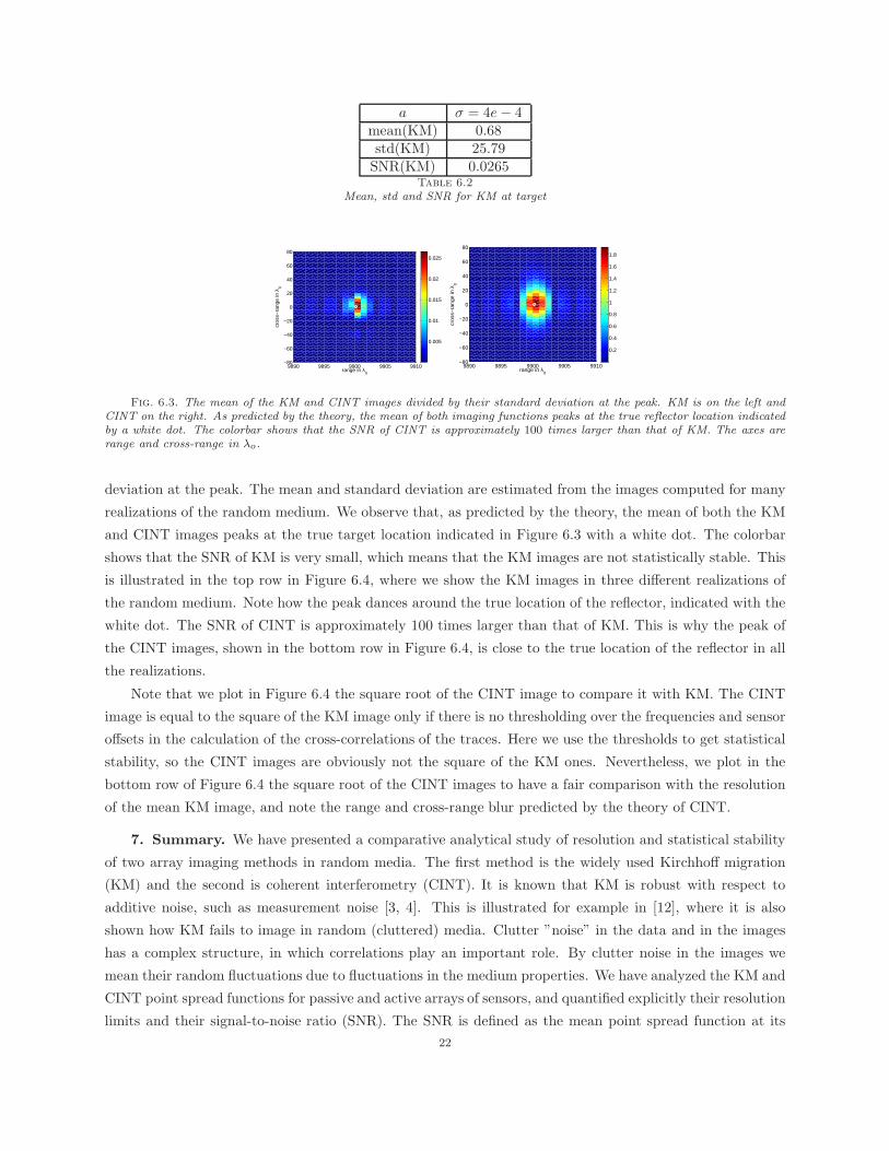
We show in Figure 6.3 the mean of the KM and CINT imaging functions, divided by their standard

21

a σ = 4e − 4mean(KM) 0.68std(KM) 25.79

SNR(KM) 0.0265Table 6.2

Mean, std and SNR for KM at target

9890 9895 9900 9905 9910−80

−60

−40

−20

0

20

40

60

80

range in λ0

cros

s−ra

nge

in λ

0

0.005

0.01

0.015

0.02

0.025

9890 9895 9900 9905 9910−80

−60

−40

−20

0

20

40

60

80

range in λ0

cros

s−ra

nge

in λ

0

0.2

0.4

0.6

0.8

1

1.2

1.4

1.6

1.8

Fig. 6.3. The mean of the KM and CINT images divided by their standard deviation at the peak. KM is on the left andCINT on the right. As predicted by the theory, the mean of both imaging functions peaks at the true reflector location indicatedby a white dot. The colorbar shows that the SNR of CINT is approximately 100 times larger than that of KM. The axes arerange and cross-range in λo.

deviation at the peak. The mean and standard deviation are estimated from the images computed for many

realizations of the random medium. We observe that, as predicted by the theory, the mean of both the KM

and CINT images peaks at the true target location indicated in Figure 6.3 with a white dot. The colorbar

shows that the SNR of KM is very small, which means that the KM images are not statistically stable. This

is illustrated in the top row in Figure 6.4, where we show the KM images in three different realizations of

the random medium. Note how the peak dances around the true location of the reflector, indicated with the

white dot. The SNR of CINT is approximately 100 times larger than that of KM. This is why the peak of

the CINT images, shown in the bottom row in Figure 6.4, is close to the true location of the reflector in all

the realizations.

Note that we plot in Figure 6.4 the square root of the CINT image to compare it with KM. The CINT

image is equal to the square of the KM image only if there is no thresholding over the frequencies and sensor

offsets in the calculation of the cross-correlations of the traces. Here we use the thresholds to get statistical

stability, so the CINT images are obviously not the square of the KM ones. Nevertheless, we plot in the

bottom row of Figure 6.4 the square root of the CINT images to have a fair comparison with the resolution

of the mean KM image, and note the range and cross-range blur predicted by the theory of CINT.

7. Summary. We have presented a comparative analytical study of resolution and statistical stability

of two array imaging methods in random media. The first method is the widely used Kirchhoff migration

(KM) and the second is coherent interferometry (CINT). It is known that KM is robust with respect to

additive noise, such as measurement noise [3, 4]. This is illustrated for example in [12], where it is also

shown how KM fails to image in random (cluttered) media. Clutter ”noise” in the data and in the images

has a complex structure, in which correlations play an important role. By clutter noise in the images we

mean their random fluctuations due to fluctuations in the medium properties. We have analyzed the KM and

CINT point spread functions for passive and active arrays of sensors, and quantified explicitly their resolution

limits and their signal-to-noise ratio (SNR). The SNR is defined as the mean point spread function at its

22

9890 9895 9900 9905 9910−80

−60

−40

−20

0

20

40

60

80

range in λ0

cros

s−ra

nge

in λ

0

9890 9895 9900 9905 9910−80

−60

−40

−20

0

20

40

60

80

range in λ0

cros

s−ra

nge

in λ

0

9890 9895 9900 9905 9910−80

−60

−40

−20

0

20

40

60

80

range in λ0

cros

s−ra

nge

in λ

0

9890 9895 9900 9905 9910−80

−60

−40

−20

0

20

40

60

80

range in λ0

cros

s−ra

nge

in λ

0

9890 9895 9900 9905 9910−80

−60

−40

−20

0

20

40

60

80

range in λ0

cros

s−ra

nge

in λ

0

9890 9895 9900 9905 9910−80

−60

−40

−20

0

20

40

60

80

range in λ0

cros

s−ra

nge

in λ

0

Fig. 6.4. Top row: KM images in three realizations of the random medium. Note how the peak dances around thetrue location of the reflector, indicated with the white dot. Bottom row: Square root of the CINT images in the same threerealizations of the random medium. Note that the peak is close to the true reflector location in all the realizations, as predictedby the theory. The axes are range and cross-range in λo.

peak divided by its standard deviation.

To carry out analytically the resolution and SNR comparative study of KM and CINT, we have used

the relatively simple random travel time model for the medium effects on the array data. The model is valid

in the regime of geometrical optics in random media. In this regime wave diffraction, amplitude fluctuations

and power delay spread due to multiple scattering are negligible, while wave front distortions are significant

and well-captured by the model. CINT and KM in random media have been studied before in [11, 9],

using the parabolic approximation model. However, an explicit analytical SNR calculation was not done in

[11, 9], because the forward scattering model is too complicated to allow evaluation of higher order statistical

moments of the array data. The results in [11, 9] agree qualitatively with those obtained in this paper.

We have focused the analysis on the case of large wave front distortions, where the random medium has

a significant effect on the imaging process. The results show that: (1) The KM and CINT imaging functions

provide an unbiased estimate of the source or reflector locations. That is to say, the statistical mean of their

point spread functions peak at the true location ~y of the sources or reflectors that we wish to image. (2)

The SNR of the KM and CINT imaging functions in the vicinity of ~y is dramatically different. The SNR

of KM is exponentially small with range, no matter how large the bandwidth or the array aperture is. This

means that KM is not statistically stable and it cannot be used for imaging in regimes with large wave front

distortions. The random fluctuations of the images are large and we cannot expect to observe the peak of

the images near ~y. The peaks dance around ~y in an unpredictable manner. The CINT imaging method is

clearly superior to KM because its SNR is not small and it is enhanced by increasing the aperture. However,

the statistical stability of CINT comes at the expense of some blurring of the images. We have quantified

explicitly the trade-off between the resolution and stability of the CINT imaging function. We have also

illustrated the theoretical results with some numerical simulations.

Acknowledgments. The work of L. Borcea was partially supported by the Office of Naval Research,

grant N00014-09-1-0290, and by the National Science Foundation, grants DMS-0907746 and DMS-0934594.

23

J. Garnier and G. Papanicolaou thank the Institut des Hautes Etudes Scientifiques (IHES) for its hospitality

while this work was completed. The work of G. Papanicolaou was partially supported by AFOSR grant

FA9550-08-1-0089. The work of C. Tsogka was partially supported by the European Research Council

Stanting Grant, GA 239959.

Appendix A. Domain of validity of the random travel time model. Within the geometric

optics approximation, the amplitude and phase perturbations of the wave are given in [21, 19] in terms of

the fluctuations of the index of refraction along the path of propagation. In this appendix we derive for

consistency these equations (see (A.1-A.2)) and we study under which conditions the random travel time

model is valid (see (A.7)).

In the geometric optics approximation, the wave has the form u = αeiωτ , where α is the amplitude and

τ is the travel time. The travel time is the solution of the eikonal equation

|∇τ |2 =1

c2(~x),

and the amplitude α is the solution of the transport equation

2∇α · ∇τ + α∆τ = 0.

If the amplitude σ of the fluctuations of the index of refraction is small, then we can expand formally

α = α0 + σα1 + σ2α2 + . . . , and τ = τ0 + στ1 + σ2τ2 + . . . .

Substituting into the eikonal and transport equations, and collecting the terms with the same powers in σ,

we find that

|∇τ0| =1

co, ∇τ0 · ∇τ1 =

µ(~x)

2c2o

,

2∇α0 · ∇τ0 + α0∆τ0 = 0, 2∇α0 · ∇τ1 + 2∇α1 · ∇τ0 + α0∆τ1 + α1∆τ0 = 0.

Let us consider the perturbation of a plane wave propagating in the xn+1 direction. To leading order

we have

α0 = 1, τ0 =xn+1

co,

and the corrections α1 and τ1 satisfy

∂xn+1τ1 =µ(~x)

2co, ∂xn+1α1 = −co

2∆τ1.

By splitting the Laplacian as ∆ = ∆⊥ + ∂2xn+1

, we find that the equation for α1 is equivalent to

∂xn+1α1 +1

4∂xn+1µ = −co

2∆⊥τ1,

which gives for ~x = (0, L),

τ1 =1

2co

∫ L

0

µ

(s~en+1

ℓ

)ds, (A.1)

α1 =1

4µ(0) − 1

4µ

(L~en+1

ℓ

)+ α1, α1 = − 1

4ℓ2

∫ L

0

(L − s)∆⊥µ

(s~en+1

ℓ

)ds. (A.2)

24

Here ~en+1 is the unit vector in Rn+1 pointing in the xn+1 direction.

Our goal is to find under which conditions the random travel time model is valid. This model says that

the amplitude perturbation of the wave is negligible, and that the phase (or travel time) perturbation can

be described in terms of a Gaussian process with mean zero. In the following lemma the hypothesis L ≫ ℓ

ensures that the statistics of τ1 is Gaussian by the central limit theorem.

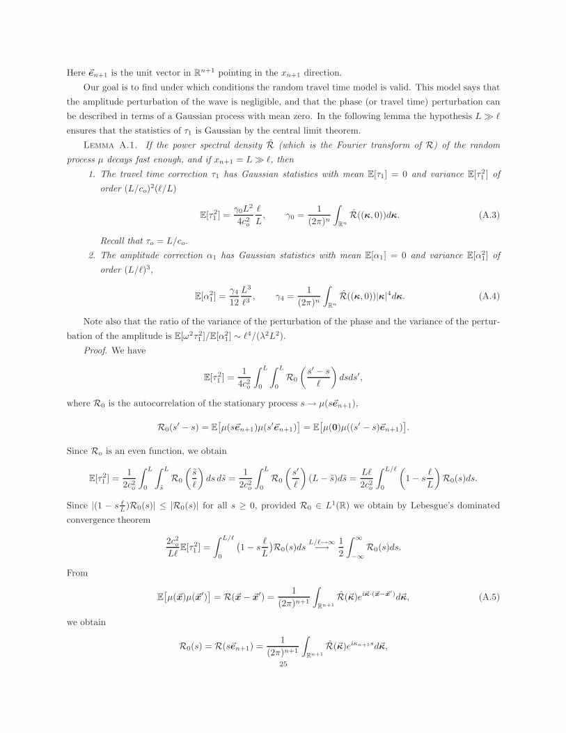
Lemma A.1. If the power spectral density R (which is the Fourier transform of R) of the random

process µ decays fast enough, and if xn+1 = L ≫ ℓ, then

1. The travel time correction τ1 has Gaussian statistics with mean E[τ1] = 0 and variance E[τ21 ] of

order (L/co)2(ℓ/L)

E[τ21 ] =

γ0L2

4c2o

ℓ

L, γ0 =

1

(2π)n

∫

Rn

R((κ, 0))dκ. (A.3)

Recall that τo = L/co.

2. The amplitude correction α1 has Gaussian statistics with mean E[α1] = 0 and variance E[α21] of

order (L/ℓ)3,

E[α21] =

γ4

12

L3

ℓ3, γ4 =

1

(2π)n

∫

Rn

R((κ, 0))|κ|4dκ. (A.4)

Note also that the ratio of the variance of the perturbation of the phase and the variance of the pertur-

bation of the amplitude is E[ω2τ21 ]/E[α2

1] ∼ ℓ4/(λ2L2).

Proof. We have

E[τ21 ] =

1

4c2o

∫ L

0

∫ L

0

R0

(s′ − s

ℓ

)dsds′,

where R0 is the autocorrelation of the stationary process s → µ(s~en+1),

R0(s′ − s) = E

[µ(s~en+1)µ(s′~en+1)

]= E

[µ(0)µ((s′ − s)~en+1)

].

Since Ro is an even function, we obtain

E[τ21 ] =

1

2c2o

∫ L

0

∫ L

s

R0

(s

ℓ

)ds ds =

1

2c2o

∫ L

0

R0

(s′

ℓ

)(L − s)ds =

Lℓ

2c2o

∫ L/ℓ

0

(1 − s

ℓ

L

)R0(s)ds.

Since |(1 − s ℓL)R0(s)| ≤ |R0(s)| for all s ≥ 0, provided R0 ∈ L1(R) we obtain by Lebesgue’s dominated

convergence theorem

2c2o

LℓE[τ2

1 ] =

∫ L/ℓ

0

(1 − s

ℓ

L

)R0(s)ds

L/ℓ→∞−→ 1

2

∫ ∞

−∞

R0(s)ds.

From

E[µ(~x)µ(~x′)

]= R(~x − ~x′) =

1

(2π)n+1

∫

Rn+1

R(~κ)ei~κ·(~x−~x′)d~κ, (A.5)

we obtain

R0(s) = R(s~en+1) =1

(2π)n+1

∫

Rn+1

R(~κ)eiκn+1sd~κ,

25

which gives result (A.3) after integrating in s.

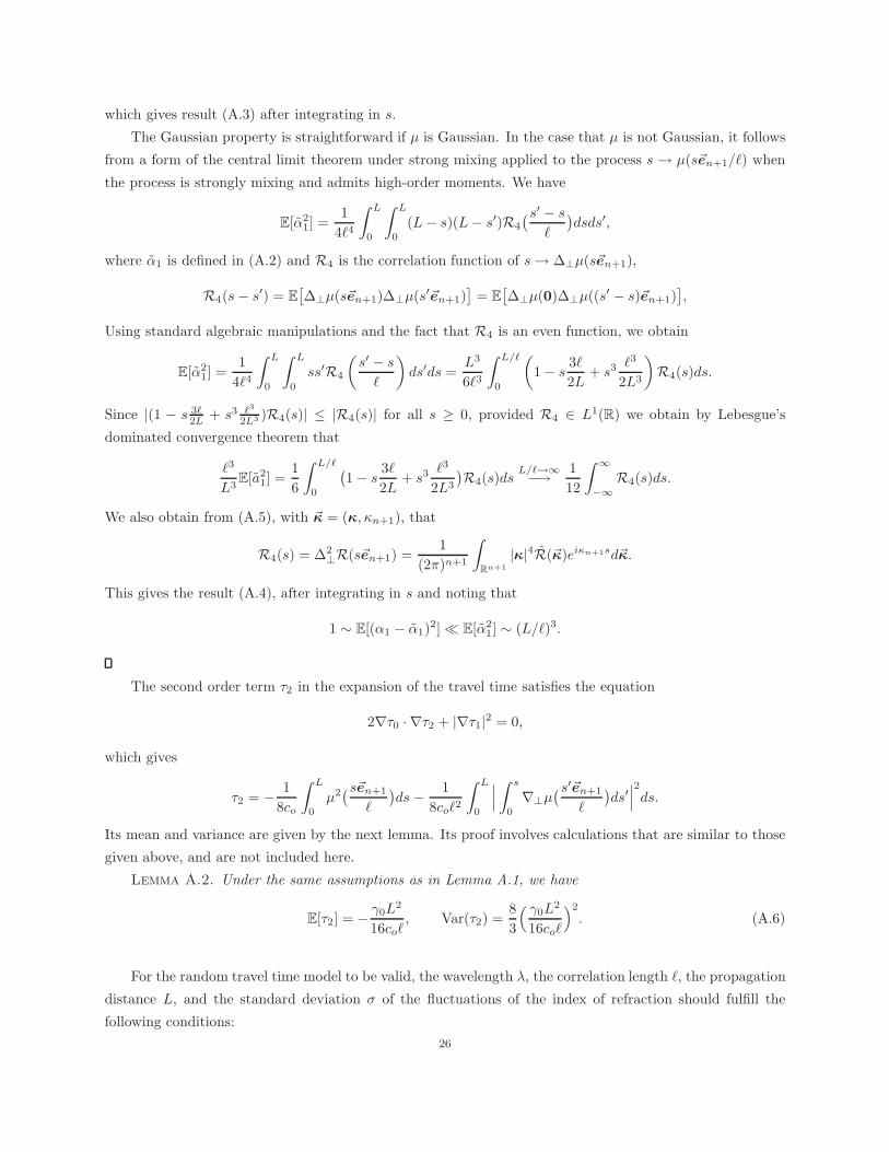
The Gaussian property is straightforward if µ is Gaussian. In the case that µ is not Gaussian, it follows

from a form of the central limit theorem under strong mixing applied to the process s → µ(s~en+1/ℓ) when

the process is strongly mixing and admits high-order moments. We have

E[α21] =

1

4ℓ4

∫ L

0

∫ L

0

(L − s)(L − s′)R4

(s′ − s

ℓ

)dsds′,

where α1 is defined in (A.2) and R4 is the correlation function of s → ∆⊥µ(s~en+1),

R4(s − s′) = E[∆⊥µ(s~en+1)∆⊥µ(s′~en+1)

]= E

[∆⊥µ(0)∆⊥µ((s′ − s)~en+1)

],

Using standard algebraic manipulations and the fact that R4 is an even function, we obtain

E[α21] =

1

4ℓ4

∫ L

0

∫ L

0

ss′R4

(s′ − s

ℓ

)ds′ds =

L3

6ℓ3

∫ L/ℓ

0

(1 − s

3ℓ

2L+ s3 ℓ3

2L3

)R4(s)ds.

Since |(1 − s 3ℓ2L + s3 ℓ3

2L3 )R4(s)| ≤ |R4(s)| for all s ≥ 0, provided R4 ∈ L1(R) we obtain by Lebesgue’s

dominated convergence theorem that

ℓ3

L3E[a2

1] =1

6

∫ L/ℓ

0

(1 − s

3ℓ

2L+ s3 ℓ3

2L3

)R4(s)ds

L/ℓ→∞−→ 1

12

∫ ∞

−∞

R4(s)ds.

We also obtain from (A.5), with ~κ = (κ, κn+1), that

R4(s) = ∆2⊥R(s~en+1) =

1

(2π)n+1

∫

Rn+1

|κ|4R(~κ)eiκn+1sd~κ.

This gives the result (A.4), after integrating in s and noting that

1 ∼ E[(α1 − α1)2] ≪ E[α2

1] ∼ (L/ℓ)3.

The second order term τ2 in the expansion of the travel time satisfies the equation

2∇τ0 · ∇τ2 + |∇τ1|2 = 0,

which gives

τ2 = − 1

8co

∫ L

0

µ2(s~en+1

ℓ

)ds − 1

8coℓ2

∫ L

0

∣∣∣∫ s

0

∇⊥µ(s′~en+1

ℓ

)ds′∣∣∣2

ds.

Its mean and variance are given by the next lemma. Its proof involves calculations that are similar to those

given above, and are not included here.

Lemma A.2. Under the same assumptions as in Lemma A.1, we have

E[τ2] = − γ0L2

16coℓ, Var(τ2) =

8

3

( γ0L2

16coℓ

)2

. (A.6)

For the random travel time model to be valid, the wavelength λ, the correlation length ℓ, the propagation

distance L, and the standard deviation σ of the fluctuations of the index of refraction should fulfill the

following conditions:

26

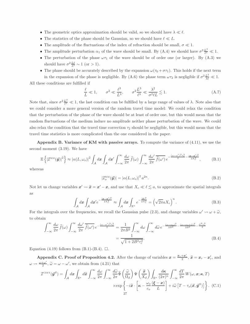
• The geometric optics approximation should be valid, so we should have λ ≪ ℓ.

• The statistics of the phase should be Gaussian, so we should have ℓ ≪ L.

• The amplitude of the fluctuations of the index of refraction should be small, σ ≪ 1.

• The amplitude perturbation α1 of the wave should be small. By (A.4) we should have σ2 L3

ℓ3 ≪ 1.

• The perturbation of the phase ωτ1 of the wave should be of order one (or larger). By (A.3) we

should have σ2 Lℓλ2 ∼ 1 (or > 1).

• The phase should be accurately described by the expansion ω(τ0 +στ1). This holds if the next term

in the expansion of the phase is negligible. By (A.6) the phase term ωτ2 is negligible if σ2 L2

λℓ ≪ 1.

All these conditions are fulfilled if

ℓ

L≪ 1, σ2 ≪ ℓ3

L3, σ2 L3

ℓ3≪ λ2

σ2ℓL. 1. (A.7)

Note that, since σ2 L3

ℓ3 ≪ 1, the last condition can be fulfilled by a large range of values of λ. Note also that

we could consider a more general version of the random travel time model: We could relax the condition

that the perturbation of the phase of the wave should be at least of order one, but this would mean that the

random fluctuations of the medium induce no amplitude neither phase perturbation of the wave. We could

also relax the condition that the travel time correction τ2 should be negligible, but this would mean that the

travel time statistics is more complicated than the one considered in the paper.

Appendix B. Variance of KM with passive arrays. To compute the variance of (4.11), we use the

second moment (3.19). We have

E

|IKM(~y)|2

≈ |α(L, ωo)|2

∫

A

dx

∫

A

dx′

∫ ∞

−∞

dω

2πf(ω)

∫ ∞

−∞

dω′

2πf(ω′) e

−(ω−ω′)2τ2

c2 − |x−x′|2

2X2c , (B.1)

whereas

|IKM

o (~y)| = |α(L, ωo)|2 a2n. (B.2)

Not let us change variables x′ x = x′ −x, and use that Xc ≪ ℓ . a, to approximate the spatial integrals

as∫

A

dx

∫

A

dx′e− |x−x′|2

2X2c ≈

∫

A

dx

∫

Rn

e− |ex|2

2X2c =

(√2πaXc

)n

. (B.3)

For the integrals over the frequencies, we recall the Gaussian pulse (2.3), and change variables ω′ ω + ω,

to obtain∫ ∞

−∞

dω

2πf(ω)

∫ ∞

−∞

dω′

2πf(ω′) e−

(ω−ω′)2τ2c

2 =1

2πB2

∫ ∞

−∞

dω

∫ ∞

−∞

dω e−(ω−ωo)2

2B2 − (ω−ωo+eω)2

2B2 −eω2τ2

c2

=1√

1 + 2B2τ2c

. (B.4)

Equation (4.19) follows from (B.1)-(B.4). .

Appendix C. Proof of Proposition 4.2. After the change of variables x =xr+x′

r

2 , x = xr −x′r, and

ω ω+ω′

2 , ω = ω − ω′, we obtain from (4.21) that

ICINT(~yS) =

∫

A

dx

∫

Rn

dx

∫ ∞

−∞

dω

2π

∫ ∞

−∞

dω

2πΦ

(ω

Ωd

)Ψ

(x

Xd

)∫

Rn

dκ

(2π)n

∫ ∞

−∞

dT

2πW (ω, x; κ, T )

×exp

−ix ·

[κ − ωo

co

(ξ − x)

L

]+ iω

[T − τo(~x, ~yS)

]. (C.1)

27

We extended the integral in x to Rn, because x is restricted by the essential support Xd of the Gaussian

window Ψ. This is assuming Xd < a. We also dropped the terms

(ω − ωo)

co

x · xL

∼ B

ωo

Xd

λoL/a,

ω|x|2coL

∼ Ωd

ωo

X2d

λoL,

based on the assumptions (4.23), and used (4.5) to get

ω

co

x · ξL

∼ Ωd

ωo

|ξ|λoL/a

≪ Ωd

B. O(1).

Now we substitute in (C.1) the Gaussian windows (2.14), integrate over x and ω and obtain

ICINT(~yS) =ΩdX

nd

(2π)n+5

2

∫

A

dx

∫ ∞

−∞

dω

∫

Rn

dκ

∫ ∞

−∞

dT W (ω, x; κ, T )

×exp

−Ω2

d [T − τo(~x, ~y)]2

2−

X2d

∣∣∣κ − ωo

co

(ξ−x)L

∣∣∣2

2

, (C.2)

as stated in Proposition 4.2. .

Appendix D. Proof of Propositions 4.3 and 4.4. Recall definitions (4.7)-(4.22), the random travel

time model (4.8), and the approximation (4.4) of the travel time, to write

E W (ω, x; κ, T ) ≈ |α(L, ωo)|2∫

Rn

dx

∫ ∞

−∞

dω f

(ω +

ω

2

)f

(ω − ω

2

)E

ei(ω+ eω

2 )ν(x+ ex2 )−i(ω− eω

2 )ν(x− ex2 )

×exp

iωτo(~x, ~y) + i

ωo

co

x · xL

+ iκ · x − iωT

. (D.1)

Here we neglected two terms in the phase,

ω

co

|x|28L

∼ Ωc

ωo

X2c

λoL, and

(ω − ωo)

co

x · xL

∼ B

ωo

Xc

λoL/a,

by the assumptions (4.25), and the fact that the mean in (D.1) is supported at frequencies |ω| . Ωc = 1/τc,

and at offsets |x| . Xc, as seen from equation (3.19). Substituting in (D.1) the Gaussian expression (2.3)

of the pulse, and the moment formula (3.19), we obtain after integrating in x and ω the expression of the

mean of the Wigner transform stated in Proposition 4.2.

The mean of ICINT(~yS) follows from (4.24) and (4.26),

EICINT(~yS)

≈ |α(L, ωo)|2Ωd(XdXc)

n

2πB2

√2B2

1 + 2B2τ2c

∫

A

dx

∫ ∞

−∞

dω e−(ω−ωo)2

B2

∫

Rn

dκ

∫ ∞

−∞

dT

×exp

−Ω2

d (T − ∆τo)2

2− T 2

2

(2B2

1 + 2B2τ2c

)− X2

c |κ|22

−X2

d

∣∣∣κ − ωo

co

ξL

∣∣∣2

2

. (D.2)

Here we used the Gaussian expression of the pulse, changed variables κ κ + ωo

co

xL , T T − τo(~x, ~y), and

introduced the difference in travel times

∆τo = τo(~x, ~yS) − τo(~x, ~y). (D.3)

28

We write next ∆τo using (4.6),

Ωd∆τo ≈ Ωdη

co− Ωd

co

x · ξL

≈ Ωdη

co, (D.4)

where the last approximation follows from (4.5),

Ωd

co

x · ξL

∼ Ωd

ωo

|ξ|λoL/a

≪ Ωd

B. 1.

The result follows by carrying out the integrals in (D.2). .

Appendix E. Variance of CINT with passive arrays. The autocorrelation of ICINT(~y) involves

the fourth order moment of the process exp(iων(xr)). Let us consider four points (xj)j=1,...,4 in A and four

frequencies (ωj)j=1,...,4 in the bandwidth. Using the Gaussian property of the process ν(x) and the fact that

C(0) = 1, we have

E[eiω1ν(x1)−iω2ν(x2)eiω3ν(x3)−iω4ν(x4)

]= exp

− τ2

c

2

[ 4∑

j=1

ω4j + 2ω1ω4C

( |x1 − x4|ℓ

)+ 2ω2ω3C

( |x2 − x3|ℓ

)

−2ω1ω2C( |x1 − x2|

ℓ

)− 2ω1ω3C

( |x1 − x3|ℓ

)− 2ω2ω4C

( |x2 − x4|ℓ

)− 2ω3ω4C

( |x3 − x4|ℓ

)].

In fact we are only interested in the forth-order moment for which the points and frequencies are of the form

ω1 = ω +ω

2, ω2 = ω − ω

2, ω3 = ω′ +

ω′

2, ω4 = ω′ − ω′

2,

x1 = x +x

2, x2 = x − x

2, x3 = x′ +

x′

2, x4 = x′ − x′

2,

with ω, ω′ = O(ωo); ω, ω′ = O(Ωd); x, x′ = O(a); x, x′ = O(Xd). If Xd ≪ ℓ, then the expression of the

forth-order moment can be simplified into

E[eiω1ν(x1)−iω2ν(x2)eiω3ν(x3)−iω4ν(x4)

]= exp

− τ2

c

2

[ω2 + ω′2 − 2ωω′C

( |x − x′|ℓ

)].

Note that a sufficient condition for Xd ≪ ℓ is that Xd ∼ Xc since Xc ≪ ℓ by Eq. (3.20). This condition

can be readilly fulfilled because we have already shown that the expectation of the CINT functional and the

resolution analysis are not affected as long as Xd ≥ Xc, so we can restrict the analysis to the second-order

moment to the case Xd ∼ Xc ≪ ℓ.

Substituting the model (4.7) of the array data in (4.21) and using the Gaussian pulse and Gaussian

windows, we have

E[ICINT(~y)ICINT(~y)

]=

|α(L, ωo)|44πB2

∫

A

dx

∫ ∞

−∞

dω

∫

Rn

dx

∫

A

dx′

∫ ∞

−∞

dω′

∫

Rn

dx′ exp

[τ2c ωω′C

( |x − x′|ℓ

)

− (ω2 + ω′2)

2

(τ2c +

1

Ω2d

+1

2B2

)− (|x|2 + |x′|2)

2

(1

X2d

+1

X2c

)],

whereas

E[ICINT(~y)

]=

|α(L, ωo)|22√

πB

∫

A

dx

∫ ∞

−∞

dω

∫

Rn

dx exp

[− ω2

2

(τ2c +

1

Ω2d

+1

2B2

)− |x|2

2

(1

X2d

+1

X2c

)].

29

Moreover, using that

exp[τ2c ωω′C

( |x − x′|ℓ

)]− 1 ≃

[τ2c ωω′C

( |x − x′|ℓ

)]+

1

2

[τ2c ωω′C

( |x − x′|ℓ

)]2,

which holds if Ωd ≪ τ−1c , we obtain the variance

Var(ICINT(~y)

)=

|α(L, ωo)|48πB2

∫

Rn

dx exp

[−|x|2

2

(1

X2d

+1

X2c

)]2

×

τ2c

∫dω ω2 exp

[−h2

2

(τ2c +

1

Ω2d

+1

2B2

)]2∫

A

dx

∫

A

dx′ C( |x − x′|

ℓ

)2

and therefore

Var [ICINT(~y)] =1

2

(τ2c

τ2c + 1

Ω2d

+ 12B2

)2 [1

a2n

∫

A

dx

∫

A

dx′ C( |x − x′|

ℓ

)2]∣∣E[ICINT(~y)

]∣∣2 .

This is the variance stated in Proposition 4.5. .

Appendix F. Proof of proposition 5.1. Let us begin with definition (5.8) of ICINT(~yS), and note

that

p(ω, xr, xs) = P(ω, xr)P(ω, xs). (F.1)

Changing the receiver variablesxr+x′

r

2 xr, xr −x′r = xr, and similar for the sources, and introducing the

central and difference frequencies ω+ω′

2 ω, ω − ω′ = ω, we have

ICINT(~yS) =

∫

A

dxr

∫

A

dxs

∫ ∞

−∞

dω

2π

∫dxrΨ

(xr

Xd

)∫dxsΨ

(xs

Xd

)∫ ∞

−∞

dω

2πΦ

(ω

Ωd

)

×P(

ω +ω

2, xr +

xr

2

)P(

ω − ω

2, xr −

xr

2

)P(

ω +ω

2, xs +

xs

2

)P(

ω − ω

2, xs −

xs

2

)

×exp−iω

[∆τo(xr, xr, ~y

S) + ∆τo(xs, xs, ~yS)]− iω

[〈τo〉 (xr, xr, ~yS) + 〈τo〉 (xs, xs, ~yS)

].(F.2)

Here we let

∆τo(xr, xr, ~yS) = τo

((xr +

xr

2, 0), ~yS

)− τo

((xr −

xr

2, 0), ~yS

)≈ xr · (xr − ξ)

coL,

〈τo〉 (xr, xr, ~yS) =

1

2

[τo

((xr +

xr

2, 0), ~yS

)+ τo

((xr −

xr

2, 0), ~yS

)]≈ τo(~xr, ~y

S) +|x|28coL

,

and used the approximation (4.6) of the travel time. By the assumption (4.23), we have

ω

co

xr · (xr − ξ)

L=

ωo

co

xr · (xr − ξ)

L+ O

(B

ωo

Xd

λoL/a

)≈ ωo

co

xr · (xr − ξ)

L,

and

ω

[τo(~xr, ~y

S) +|x|28coL

]= ωτo(~xr, ~y

S) + O

(Ωd

ωo

X2d

λoL

)≈ ωτo(~xr, ~y

S),

so (F.2) becomes

ICINT(~yS) ≈∫

A

dxr

∫

A

dxs

∫ ∞

−∞

dω

2π

∫dxrΨ

(xr

Xd

)∫dxsΨ

(xs

Xd

)∫ ∞

−∞

dω

2πΦ

(ω

Ωd

)

×P(

ω +ω

2, xr +

xr

2

)P(

ω − ω

2, xr −

xr

2

)e−i ωo

co

exr ·(xr−ξ)L

−ieωτo(~xr,~yS)

×P(

ω +ω

2, xs +

xs

2

)P(

ω − ω

2, xs −

xs

2

)e−i ωo

co

exs·(xs−ξ)L

−ieωτo(~xs,~yS). (F.3)

30

Now let us write PP in terms of the Wigner transform, and use the Gaussian windows to obtain

ICINT(~yS) ≈ 1

(2π)2n+4

∫

A

dxr

∫

A

dxs

∫ ∞

−∞

dω

∫dκr

∫dTr W(ω, xr; κr, Tr)

∫dκs

∫dTs W(ω, xs; κs, Ts)

×∫

dxr e− |exr|2

2X2d

−iexr·(κr−ωoco

(ξ−xr)L )

∫dxs e

− |exs|2

2X2d

−iexr ·(κs−ωoco

(ξ−xs)L )

×∫

dωe− eω2

2Ω2d

+ieω[Tr+Ts−τo(~xr,~yS)−τo(~xs,~yS)].

Proposition 5.1 follows by integration over xr, xs and ω. .

REFERENCES

[1] R.J. Adler, The geometry of random fields, Wiley, London, 1981.[2] R. Alonso, L. Borcea, G. Papanicolaou, and C. Tsogka, Detection and imaging in strongly backscattering randomly

layered media, Inverse Problems, 27 (2011), p. 025004(43pp.).[3] H. Ammari, J. Garnier, H. Kang, W.K. Park, and K. Solna, Imaging schemes for perfectly conducting cracks, SIAM

J. Appl. Math., 71 (2011), pp. 68–91.[4] H. Ammari, J. Garnier, and K. Solna, A statistical approach to target detection and localization in the presence of

noise, Waves in Random and Complex Media, (to appear).[5] B. Biondi, 3D seismic imaging, Society of Exploration Geophysics, Tulsa, 2006.[6] N. Bleistein, J.K. Cohen, and J.W. Stockwell, Mathematics of multidimensional seismic imaging, migration, and

inversion, Springer, New York, 2001.[7] L. Borcea, J. Garnier, G. Papanicolaou, and C. Tsogka, Coherent interferometric imaging, time gating, and beam-

forming. submitted in 2010 to Inverse Problems.[8] L. Borcea, G. Papanicolaou, and C. Tsogka, Interferometric array imaging in clutter, Inverse Problems, 21 (2005),

pp. 1419–1460.[9] , Adaptive interferometric imaging in clutter and optimal illumination, Inverse Problems, 22 (2006), pp. 1405–1436.

[10] , Coherent interferometric imaging in clutter, Geophysics, 71 (2006), pp. SI165–SI175.[11] , Asymptotics for the space-time Wigner transform with applications to imaging, Stochastic Differential Equations:

Theory and Applications. Volume in Honor of Professor Boris L Rozovskii, PH Baxendale and SV Lototsky editors.,Interdisciplinary Mathematical Sciences, 2 (2007).

[12] , Adaptive Time-Frequency Detection and Filtering for Imaging in Heavy Clutter, SIAM Imaging Science, (to appear2011).

[13] M. Born and E. Wolf, Principles of optics: Electromagnetic theory of propagation, interference and diffraction of light,Cambridge University Press, Cambridge, 7 ed., 1999.

[14] J.C. Curlander and R.N. McDonough, Synthetic aperture radar: systems and signal processing, Wiley, New York,1991.

[15] L.J. Fradkin, Limits of validity of geometrical optics in weakly irregular media, J. Opt. Soc. Am. A, 6 (1989), pp. 1315–1319.

[16] J.W. Hardy, Adaptive optics for astronomical telescopes, Oxford University Press, USA, 1998.[17] G. Matheron, Principles of geostatistics, Economic Geology, 58 (1963), pp. 1246–1266.[18] B.D. Ripley, Spatial statistics, Wiley-Blackwell, Hoboken, 2004.[19] S.M. Rytov, Y.A. Kravtsov, and V.I. Tatarskii, Principles of statistical radiophysics. 4. Wave Propagation through

random media, Springer Verlag, Berlin, 1989.[20] L. Ryzhik, G. Papanicolaou, and J.B. Keller, Transport equations for elastic and other waves in random media, Wave

motion, 24 (1996), pp. 327–370.[21] V.I. Tatarski, Wave propagation in a turbulent medium, Dover, New York, 1961.[22] R. Tyson, Principles of adaptive optics, CRC Press, Boca Raton, 2010.[23] B.S. White, The stochastic caustic, SIAM J. Appl. Math., 44 (1984), pp. 127–149.

31