Statistical Forecasting Workshop
208
Statistical Forecasting Workshop
-
Upload
independent -
Category
Documents
-
view
0 -
download
0
Transcript of Statistical Forecasting Workshop
Statistical Forecasting Workshop
Workshop ContentsWorkshop ContentsDay 1Day 1
•• Introduction to Business ForecastingIntroduction to Business Forecasting
•• Introduction to Time Series, Simple Introduction to Time Series, Simple Averages, Moving Averages and Averages, Moving Averages and Exponential SmoothingExponential Smoothing
2
Exponential SmoothingExponential Smoothing
•• Regression Models for ForecastingRegression Models for Forecasting
•• Forecasting AccuracyForecasting Accuracy
•• Putting it all Together Putting it all Together –– The Forecasting The Forecasting ProcessProcess
• Basic statistics review
• Autocorrelation and Partial Autocorrelation
• The family of ARIMA models– Autoregressive
– Moving average
Workshop ContentsWorkshop ContentsDay 2Day 2
– Moving average
– Differencing
– Seasonal Autoregressive
– Seasonal moving average
– Seasonal differencing
– Transfer functions
• The general ARIMA model
• The modeling process
• Example of the modeling process–General Mills biscuits
– Univariate model
– Regression model
Workshop ContentsWorkshop ContentsDay 2 (continued)Day 2 (continued)
– Regression model
– ARIMA transfer function model
– Modeling outliers
• Another example – daily sales of a beer brand and package at one grocery store
Workshop ObjectivesWorkshop Objectives
•• This workshop is designed to provide you This workshop is designed to provide you with an understanding and conceptual with an understanding and conceptual basis for some basic time series basis for some basic time series forecasting models.forecasting models.
5
•• We will demonstrate these models using We will demonstrate these models using MS Excel. MS Excel.
•• You will be able to make forecasts of You will be able to make forecasts of business / market variables with greater business / market variables with greater accuracy than you may be experiencing accuracy than you may be experiencing now.now.
1. Introduction to 1. Introduction to Business ForecastingBusiness ForecastingBusiness ForecastingBusiness Forecasting
Why Forecast?Why Forecast?
•• Make best use of resources byMake best use of resources by
–– Developing future plansDeveloping future plans
–– Planning cash flow to prevent shortfallsPlanning cash flow to prevent shortfalls
–– Achieving competitive delivery timesAchieving competitive delivery times
7
–– Achieving competitive delivery timesAchieving competitive delivery times
–– Supporting business financial objectivesSupporting business financial objectives
–– Reducing uncertaintyReducing uncertainty
What Is Riding On The Forecast?What Is Riding On The Forecast?
•• Allocation of resources:Allocation of resources:
–– InvestmentsInvestments
–– CapitalCapital
–– InventoryInventory
8
–– InventoryInventory
–– CapacityCapacity
–– Operations budgetsOperations budgets
–– Marketing budgetMarketing budget
–– Manpower and hiringManpower and hiring

Who Needs The Forecast?Who Needs The Forecast?
•• The people who allocate resourcesThe people who allocate resources
–– MarketingMarketing
–– SalesSales
–– FinanceFinance
9
–– FinanceFinance
–– ProductionProduction
–– Supply chainSupply chain
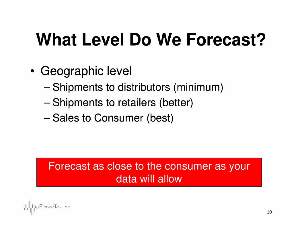
What Level Do We Forecast?What Level Do We Forecast?
•• Geographic levelGeographic level
–– Shipments to distributors (minimum)Shipments to distributors (minimum)
–– Shipments to retailers (better)Shipments to retailers (better)
–– Sales to Consumer (best)Sales to Consumer (best)
10
–– Sales to Consumer (best)Sales to Consumer (best)
Forecast as close to the consumer as your data will allow
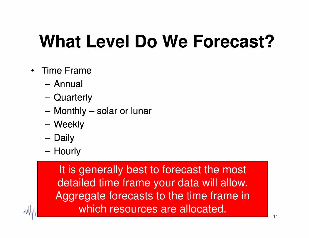
What Level Do We Forecast?What Level Do We Forecast?
•• Time FrameTime Frame
–– AnnualAnnual
–– QuarterlyQuarterly
–– Monthly Monthly –– solar or lunarsolar or lunar
–– WeeklyWeekly
11
–– WeeklyWeekly
–– DailyDaily
–– HourlyHourly
It is generally best to forecast the most detailed time frame your data will allow. Aggregate forecasts to the time frame in
which resources are allocated.
What Do We Know About What Do We Know About Forecasts?Forecasts?
•• Forecasts are always wrongForecasts are always wrong•• Error estimates for forecasts are imperative.Error estimates for forecasts are imperative.•• Good forecasts require a firm knowledge of the process Good forecasts require a firm knowledge of the process
being forecast.being forecast.•• It is essential that there be a business process in place It is essential that there be a business process in place
to use the forecast. Otherwise it will never be used.to use the forecast. Otherwise it will never be used.
12
to use the forecast. Otherwise it will never be used.to use the forecast. Otherwise it will never be used.•• Forecasts are more accurate for larger groups of itemsForecasts are more accurate for larger groups of items•• Forecasts are more accurate for longer time periods. Forecasts are more accurate for longer time periods.
E.g. annual forecasts are more accurate than monthly, E.g. annual forecasts are more accurate than monthly, which are more accurate than weekly, and so on.which are more accurate than weekly, and so on.
•• Forecasts are generally more accurate for fewer future Forecasts are generally more accurate for fewer future time periodstime periods
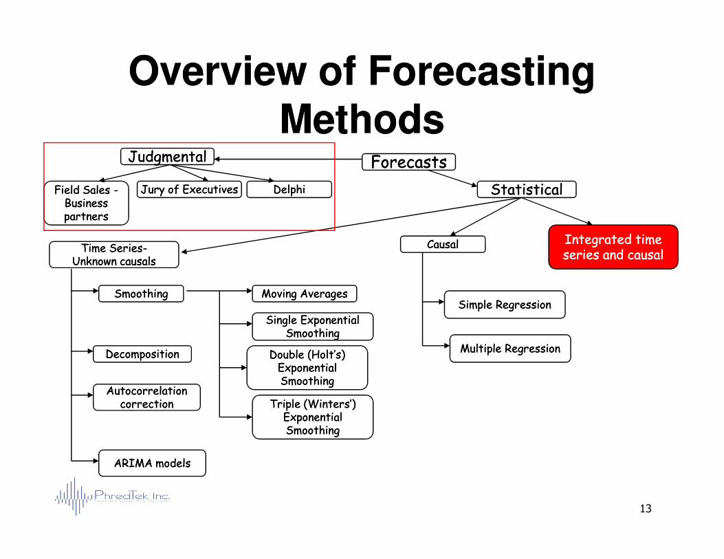
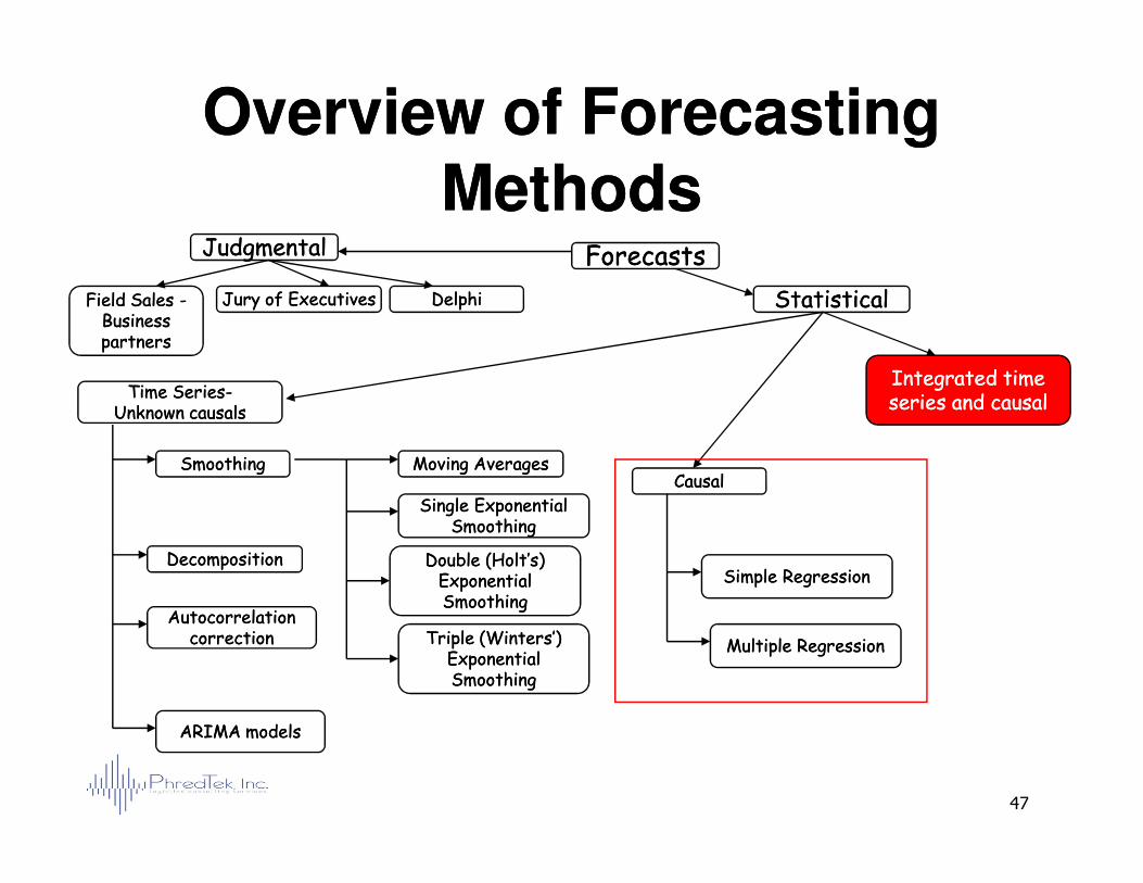
Overview of Forecasting Overview of Forecasting MethodsMethods
ForecastsForecastsJudgmentalJudgmental
StatisticalStatistical
CausalCausalTime SeriesTime Series--Unknown causalsUnknown causals
Integrated time Integrated time series and causalseries and causal
DelphiDelphiJury of ExecutivesJury of ExecutivesField Sales Field Sales --Business Business partnerspartners
13
Autocorrelation Autocorrelation correctioncorrection
DecompositionDecomposition
SmoothingSmoothing Moving AveragesMoving Averages
Single Exponential Single Exponential SmoothingSmoothing
Double (Holt’s) Double (Holt’s) Exponential Exponential SmoothingSmoothing
Triple (Winters’) Triple (Winters’) Exponential Exponential SmoothingSmoothing
Simple RegressionSimple Regression
Multiple RegressionMultiple Regression
ARIMA modelsARIMA models
Judgmental ForecastsJudgmental ForecastsSales Force and Business Partners Sales Force and Business Partners
•• These people often understand nuances of the These people often understand nuances of the marketplace that effect sales.marketplace that effect sales.
•• Are motivated to produce good forecasts Are motivated to produce good forecasts because it effects their workload.because it effects their workload.
•• Can be biased for personal gain.Can be biased for personal gain.
14
•• Can be biased for personal gain.Can be biased for personal gain.•• An effective alternative is to provide them with a An effective alternative is to provide them with a
statistical based forecast and ask them to adjust statistical based forecast and ask them to adjust it.it.
Judgmental ForecastsJudgmental ForecastsJury of Executive OpinionJury of Executive Opinion
•• An An executive generally knows more about the executive generally knows more about the business than a forecaster.business than a forecaster.
•• Executives are strongly motivated to produce Executives are strongly motivated to produce good forecasts because their performance is good forecasts because their performance is
15
good forecasts because their performance is good forecasts because their performance is dependent on them.dependent on them.
•• However, executives can also be biased for However, executives can also be biased for personal gain.personal gain.
•• An alternative is to provide them with a statistical An alternative is to provide them with a statistical forecast and ask them to adjust it. forecast and ask them to adjust it.
Judgmental ForecastsJudgmental ForecastsDelphi MethodDelphi Method
Six Steps:Six Steps:1.1. Participating panel members are selected.Participating panel members are selected.2.2. Questionnaires asking for opinions about the variables Questionnaires asking for opinions about the variables
to be forecast are distributed to panel members.to be forecast are distributed to panel members.3.3. Results from panel members are collected, tabulated, Results from panel members are collected, tabulated,
and summarized.and summarized.
16
and summarized.and summarized.4.4. Summary results are distributed to the panel members Summary results are distributed to the panel members
for their review and consideration.for their review and consideration.5.5. Panel members revise their individual estimates, taking Panel members revise their individual estimates, taking
account of the information received from the other, account of the information received from the other, unknown panel members.unknown panel members.
6.6. Steps 3 through 5 are repeated until no significant Steps 3 through 5 are repeated until no significant changes result.changes result.
Time Series ModelsTime Series Models
•• Naïve ForecastNaïve Forecast–– Tomorrow will be the same as todayTomorrow will be the same as today
•• Moving AveraqeMoving Averaqe–– Unweighted Linear Combination of Past Actual Unweighted Linear Combination of Past Actual
ValuesValues
17
ValuesValues
•• Exponential SmoothingExponential Smoothing–– Weighted Linear Combination of Past Actual ValuesWeighted Linear Combination of Past Actual Values
•• DecompositionDecomposition–– Break time series into trend, seasonality, and Break time series into trend, seasonality, and
randomness.randomness.
Causal/Explanatory ModelsCausal/Explanatory Models
•• Simple Regression:Simple Regression:
–– Variations in dependent variable is explained Variations in dependent variable is explained by one independent variable.by one independent variable.
18
•• Multiple Regression:Multiple Regression:
–– Variations in dependent variable is explained Variations in dependent variable is explained by multiple independent variables.by multiple independent variables.
2. Time Series Methods 2. Time Series Methods
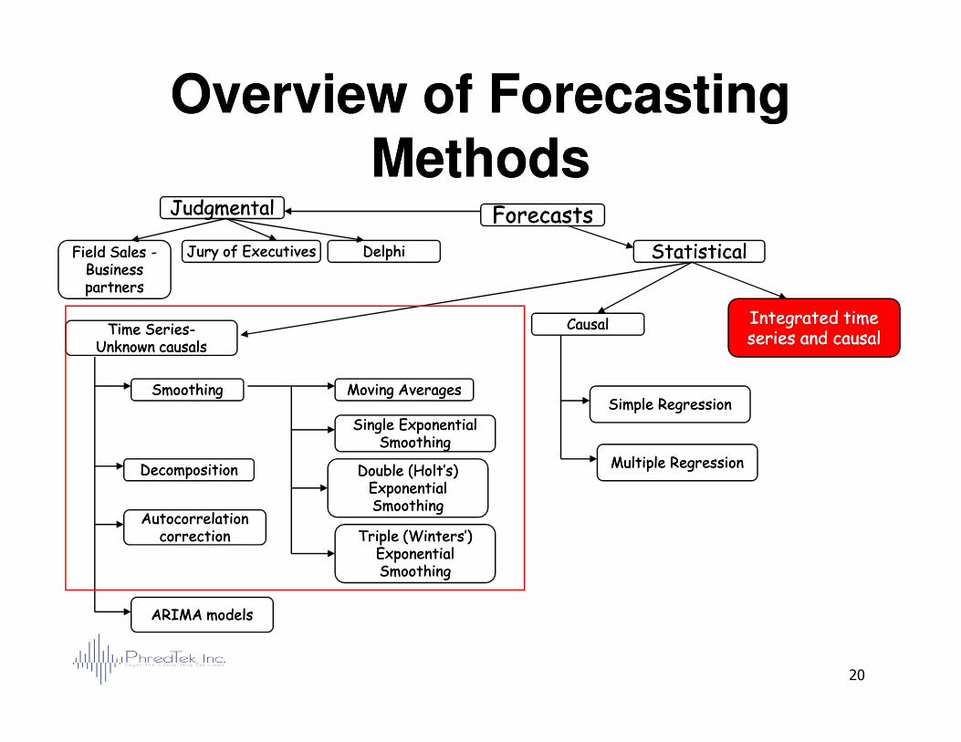
Overview of Forecasting Overview of Forecasting MethodsMethods
ForecastsForecastsJudgmentalJudgmental
StatisticalStatistical
CausalCausalTime SeriesTime Series--Unknown causalsUnknown causals
Integrated time Integrated time series and causalseries and causal
DelphiDelphiJury of ExecutivesJury of ExecutivesField Sales Field Sales --Business Business partnerspartners
20
Autocorrelation Autocorrelation correctioncorrection
DecompositionDecomposition
SmoothingSmoothing Moving AveragesMoving Averages
Single Exponential Single Exponential SmoothingSmoothing
Double (Holt’s) Double (Holt’s) Exponential Exponential SmoothingSmoothing
Triple (Winters’) Triple (Winters’) Exponential Exponential SmoothingSmoothing
Simple RegressionSimple Regression
Multiple RegressionMultiple Regression
ARIMA modelsARIMA models
Naïve ModelNaïve Model
•• Special Case of Single Exponential Special Case of Single Exponential SmoothingSmoothing
•• Forecast Value is equal to the Previously Forecast Value is equal to the Previously
21
•• Forecast Value is equal to the Previously Forecast Value is equal to the Previously Observed ValueObserved Value
–– Stable EnvironmentStable Environment
–– Slow Rate of Change (if any)Slow Rate of Change (if any)
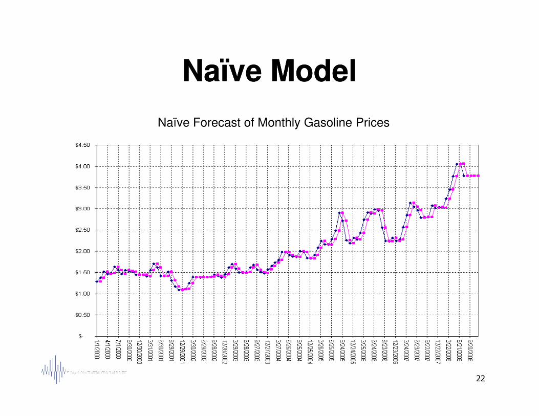
Naïve ModelNaïve Model
Naïve Forecast of Monthly Gasoline Prices
22
Why Use The Naïve Model?Why Use The Naïve Model?
•• It’s safe. It will never forecast a value that It’s safe. It will never forecast a value that hasn’t happened before.hasn’t happened before.
•• It is useful for comparing the quality of It is useful for comparing the quality of
23
•• It is useful for comparing the quality of It is useful for comparing the quality of other forecasting models. If forecast error other forecasting models. If forecast error of another method is higher than the naïve of another method is higher than the naïve model, it’s not very good.model, it’s not very good.
Moving Average ModelMoving Average Model
•• Easy to CalculateEasy to Calculate–– Select Number of PeriodsSelect Number of Periods
–– Apply to ActualApply to Actual
•• Assimilates Actual ExperienceAssimilates Actual Experience
24
•• Assimilates Actual ExperienceAssimilates Actual Experience
•• Absorbs Recent ChangeAbsorbs Recent Change
•• Smoothes Forecast in Face of Random Smoothes Forecast in Face of Random VariationVariation
•• Safe Safe –– never forecasts outside historical never forecasts outside historical values.values.
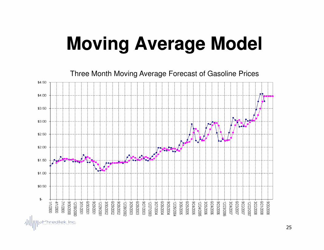
Moving Average ModelMoving Average Model
Three Month Moving Average Forecast of Gasoline Prices
25
Time Series Methods Time Series Methods ––Exponential SmoothingExponential Smoothing
•• Single Exponential SmoothingSingle Exponential Smoothing
•• Double Double -- Holt’s Exponential SmoothingHolt’s Exponential Smoothing
•• Winters’ Exponential SmoothingWinters’ Exponential Smoothing
26
Exponential SmoothingExponential Smoothing
•• Widely UsedWidely Used
•• Easy to CalculateEasy to Calculate
•• Limited Data RequiredLimited Data Required
•• Assumes Random Variation Around a Assumes Random Variation Around a
27
•• Assumes Random Variation Around a Assumes Random Variation Around a Stable LevelStable Level
•• Expandable to Trend Model and to Expandable to Trend Model and to Seasonal ModelSeasonal Model
Smoothing ParametersSmoothing Parameters
•• Level (Randomness) Level (Randomness) –– Simple ModelSimple Model
–– Assumes variation around a levelAssumes variation around a level
•• Trend Trend –– Holt’s ModelHolt’s Model
–– Assumes linear trend in dataAssumes linear trend in data
28
–– Assumes linear trend in dataAssumes linear trend in data
•• Seasonality Seasonality –– Winter’s ModelWinter’s Model
–– Assumes recurring pattern in periodicity due Assumes recurring pattern in periodicity due to seasonal factorsto seasonal factors
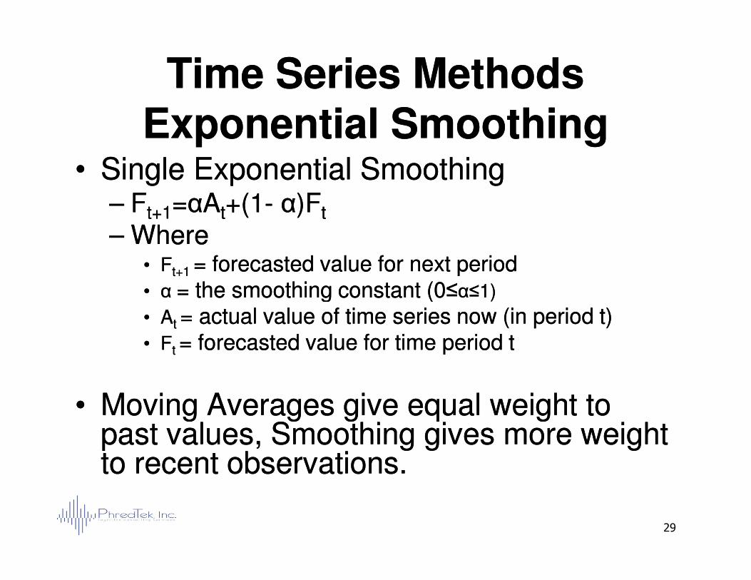
Time Series MethodsTime Series MethodsExponential SmoothingExponential Smoothing
•• Single Exponential SmoothingSingle Exponential Smoothing–– FFt+1t+1==ααAAtt+(1+(1-- αα)F)Ftt
–– WhereWhere•• FFt+1 t+1 = forecasted value for next period= forecasted value for next period•• α α = the smoothing constant (0≤= the smoothing constant (0≤αα≤1)≤1)
29
•• α α = the smoothing constant (0≤= the smoothing constant (0≤αα≤1)≤1)
•• AAt t = actual value of time series now (in period t)= actual value of time series now (in period t)•• FFt t = forecasted value for time period t= forecasted value for time period t
•• Moving Averages give equal weight to Moving Averages give equal weight to past values, Smoothing gives more weight past values, Smoothing gives more weight to recent observations.to recent observations.
Time Series MethodsTime Series MethodsExponential SmoothingExponential Smoothing
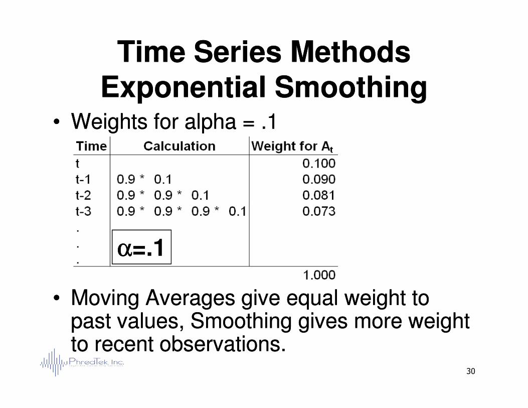
•• Weights for alpha = .1Weights for alpha = .1
30
•• Moving Averages give equal weight to Moving Averages give equal weight to past values, Smoothing gives more weight past values, Smoothing gives more weight to recent observations.to recent observations.
αααα=.1αααα=.1
Time Series MethodsTime Series MethodsExponential SmoothingExponential Smoothing
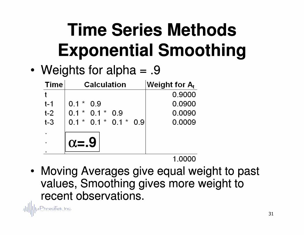
•• Weights for alpha = .9Weights for alpha = .9
31
•• Moving Averages give equal weight to past Moving Averages give equal weight to past values, Smoothing gives more weight to values, Smoothing gives more weight to recent observations.recent observations.
αααα=.9
Time Series MethodsTime Series MethodsExponential SmoothingExponential Smoothing
•• The Single The Single Exponential Exponential Smoothing Rule of Smoothing Rule of ThumbThumb
•• The closer to 1 the The closer to 1 the value of alpha, the value of alpha, the more strongly the more strongly the forecast depends forecast depends
32
ThumbThumb forecast depends forecast depends upon recent values.upon recent values.
In actual practice, In actual practice, alpha values from 0.05 to alpha values from 0.05 to 0.30 work very well 0.30 work very well in most Single smoothing in most Single smoothing models. If a value of greater than 0.30 gives the models. If a value of greater than 0.30 gives the best fit this usually indicates that another best fit this usually indicates that another forecasting technique would work even better.forecasting technique would work even better.
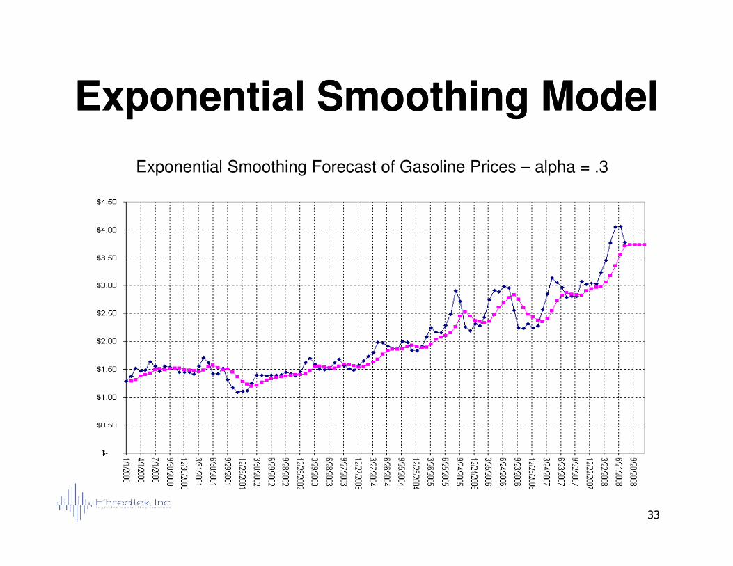
Exponential Smoothing ModelExponential Smoothing Model
Exponential Smoothing Forecast of Gasoline Prices – alpha = .3
33
Time Series MethodsTime Series MethodsExponential SmoothingExponential Smoothing
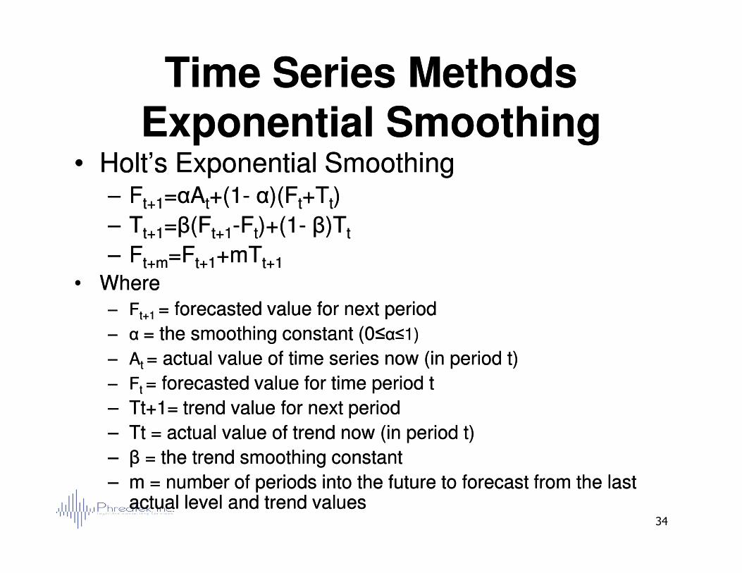
•• Holt’s Exponential SmoothingHolt’s Exponential Smoothing–– FFt+1t+1==ααAAtt+(1+(1-- αα)(F)(Ftt+T+Ttt))
–– TTt+1t+1==ββ(F(Ft+1t+1--FFtt)+(1)+(1-- ββ)T)Ttt
–– FFt+mt+m=F=Ft+1t+1+mT+mTt+1t+1
•• WhereWhere
34
•• WhereWhere–– FFt+1 t+1 = forecasted value for next period= forecasted value for next period
–– α α = the smoothing constant (0≤= the smoothing constant (0≤αα≤1)≤1)
–– AAt t = actual value of time series now (in period t)= actual value of time series now (in period t)
–– FFt t = forecasted value for time period t= forecasted value for time period t
–– Tt+1= trend value for next periodTt+1= trend value for next period
–– Tt = actual value of trend now (in period t)Tt = actual value of trend now (in period t)
–– ββ = the trend smoothing constant= the trend smoothing constant
–– m = number of periods into the future to forecast from the last m = number of periods into the future to forecast from the last actual level and trend valuesactual level and trend values
Time Series MethodsTime Series MethodsExponential SmoothingExponential Smoothing
•• Holt’s Exponential SmoothingHolt’s Exponential Smoothing
–– Used Used for data exhibiting a trend over time (for data exhibiting a trend over time (±±))
–– Data display nonData display non--seasonal patternseasonal pattern
–– Involves two smoothing factors (constants), a Involves two smoothing factors (constants), a
35
–– Involves two smoothing factors (constants), a Involves two smoothing factors (constants), a single smoothing factor and trend smoothing single smoothing factor and trend smoothing factorfactor
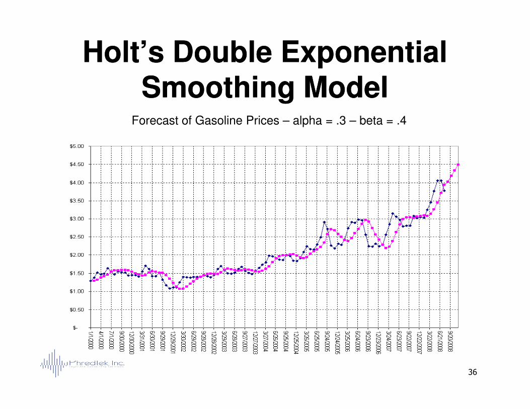
Holt’s Double Exponential Holt’s Double Exponential Smoothing ModelSmoothing Model
Forecast of Gasoline Prices – alpha = .3 – beta = .4
36
Time Series MethodsTime Series MethodsExponential SmoothingExponential Smoothing
•• Winters’ Exponential SmoothingWinters’ Exponential Smoothing
–– Adjusts for both trend and seasonalityAdjusts for both trend and seasonality
–– Even more complex calculations but also Even more complex calculations but also simple to apply using softwaresimple to apply using software
37
simple to apply using softwaresimple to apply using software
–– Involves the use of three smoothing Involves the use of three smoothing parameters, a single smoothing parameter, a parameters, a single smoothing parameter, a trend smoothing parameter, and a seasonality trend smoothing parameter, and a seasonality smoothing parametersmoothing parameter
Time Series MethodsTime Series MethodsExponential SmoothingExponential Smoothing
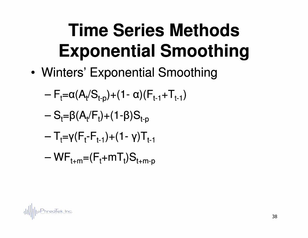
•• Winters’ Exponential SmoothingWinters’ Exponential Smoothing
–– FFtt==αα(A(Att/S/Stt--pp)+(1)+(1-- αα)(F)(Ftt--11+T+Ttt--11))
–– SStt==ββ(A(Att/F/Ftt)+(1)+(1--ββ)S)Stt--pp
38
–– SStt==ββ(A(Att/F/Ftt)+(1)+(1--ββ)S)Stt--pp
–– TTtt==γγ(F(Ftt--FFtt--11)+(1)+(1-- γγ)T)Ttt--11
–– WFWFt+mt+m=(F=(Ftt+mT+mTtt)S)St+mt+m--pp
Time Series MethodsTime Series MethodsExponential SmoothingExponential Smoothing
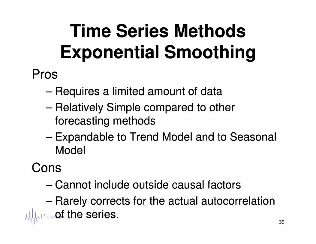
ProsPros
–– Requires a limited amount of dataRequires a limited amount of data
–– Relatively Simple compared to other Relatively Simple compared to other forecasting methodsforecasting methods
39
forecasting methodsforecasting methods
–– Expandable to Trend Model and to Seasonal Expandable to Trend Model and to Seasonal ModelModel
ConsCons
–– Cannot include outside causal factorsCannot include outside causal factors
–– Rarely corrects for the actual autocorrelation Rarely corrects for the actual autocorrelation of the series.of the series.
Time Series DecompositionTime Series Decomposition
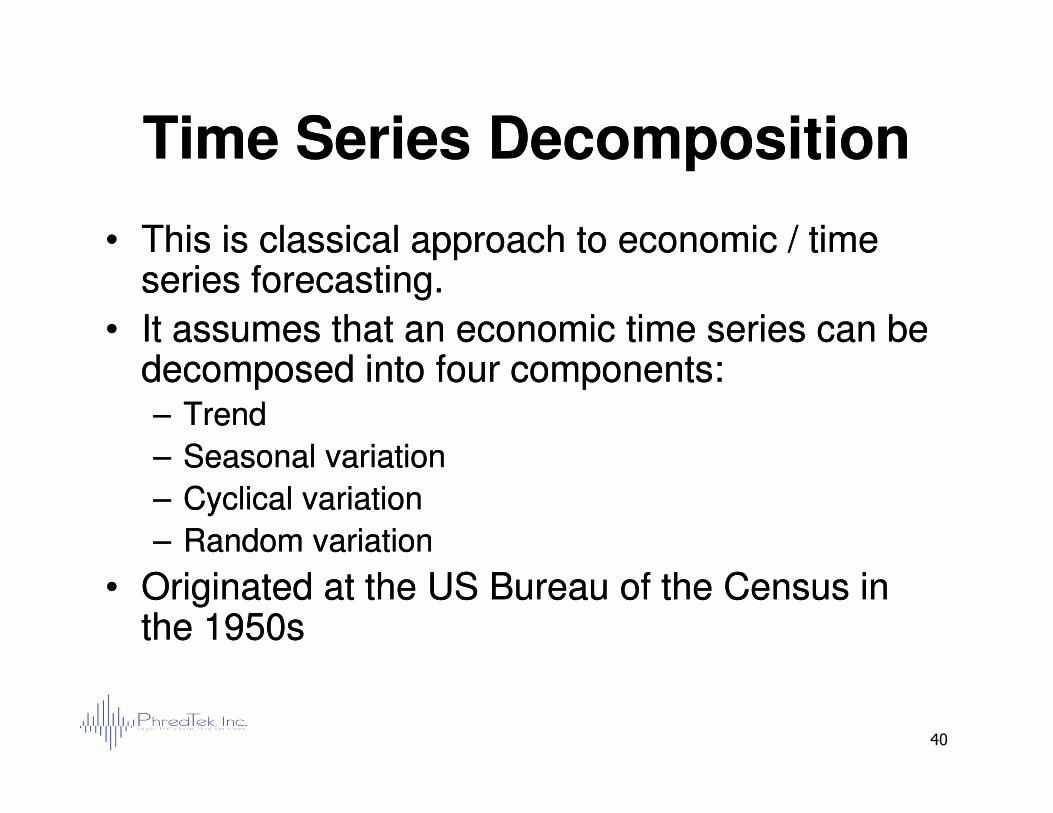
•• This is classical approach to economic / time This is classical approach to economic / time series forecasting.series forecasting.
•• It assumes that an economic time series can be It assumes that an economic time series can be decomposed into four components:decomposed into four components:–– TrendTrend
40
–– TrendTrend
–– Seasonal variationSeasonal variation
–– Cyclical variationCyclical variation
–– Random variationRandom variation
•• Originated at the US Bureau of the Census in Originated at the US Bureau of the Census in the 1950sthe 1950s
Time Series DecompositionTime Series Decomposition
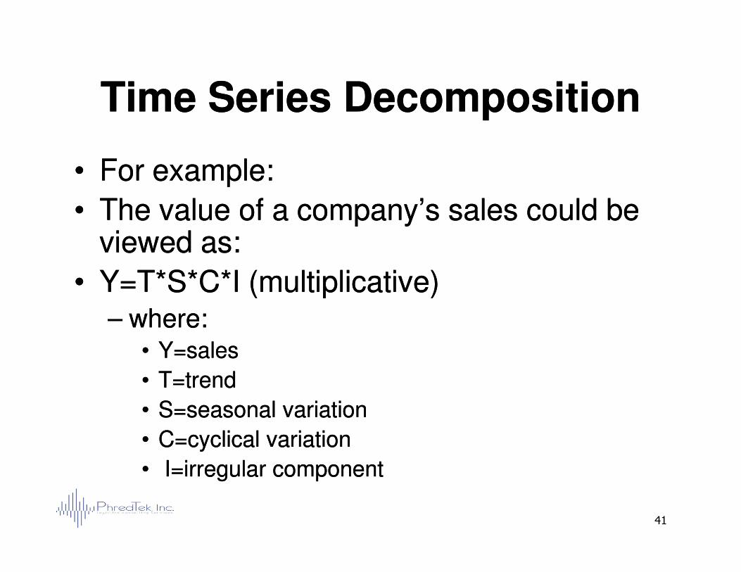
•• For example:For example:
•• The value of a company’s sales could be The value of a company’s sales could be viewed as:viewed as:
•• Y=T*S*C*I (multiplicative)Y=T*S*C*I (multiplicative)
41
•• Y=T*S*C*I (multiplicative)Y=T*S*C*I (multiplicative)–– where:where:
•• Y=salesY=sales
•• T=trendT=trend
•• S=seasonal variationS=seasonal variation
•• C=cyclical variationC=cyclical variation
•• I=irregular I=irregular componentcomponent
Classical Decomposition Classical Decomposition ModelModel
•• A different approach to forecasting A different approach to forecasting seasonal data seriesseasonal data series
–– Calculate the seasonals for the seriesCalculate the seasonals for the series
–– DeDe--seasonalize the raw dataseasonalize the raw data
42
–– DeDe--seasonalize the raw dataseasonalize the raw data
–– Apply the forecasting methodApply the forecasting method
–– ReRe--sesonalize the seriessesonalize the series
Classical Decomposition ModelClassical Decomposition ModelPractical Practical ApplicationApplication
•• US Bureau of the Census developed X11 US Bureau of the Census developed X11 procedure during the 1950s.procedure during the 1950s.
•• This is the most widely used method.This is the most widely used method.
•• USBOC developed Fortran code to USBOC developed Fortran code to
43
•• USBOC developed Fortran code to USBOC developed Fortran code to implement. implement. –– Still available if you search Still available if you search hard.hard.
•• SAS has a PROC X11.SAS has a PROC X11.
•• Only works well for very stable processes Only works well for very stable processes that don’t change much over time.that don’t change much over time.
Summary of Time Series Summary of Time Series ForecastingForecasting
•• Should be used when a limited amount of Should be used when a limited amount of data is available on external factors data is available on external factors (factors other than actual history), (factors other than actual history), e.g., e.g., price changes, economic activity, etc. price changes, economic activity, etc.
44
price changes, economic activity, etc. price changes, economic activity, etc.
•• Useful when trend rates, seasonal Useful when trend rates, seasonal patterns, and level changes are presentpatterns, and level changes are present
•• Otherwise, Causal/Explanatory techniques Otherwise, Causal/Explanatory techniques may be more appropriate.may be more appropriate.

Excel ExerciseExcel ExerciseExcel ExerciseExcel Exercise
3. Cause3. Cause--andand--Effect Effect Models Models Models Models
Regression ForecastingRegression Forecasting
Overview of Forecasting Overview of Forecasting MethodsMethods
ForecastsForecastsJudgmentalJudgmental
StatisticalStatistical
Time SeriesTime Series--Unknown causalsUnknown causals
Integrated time Integrated time series and causalseries and causal
DelphiDelphiJury of ExecutivesJury of ExecutivesField Sales Field Sales --Business Business partnerspartners
47
CausalCausal
Autocorrelation Autocorrelation correctioncorrection
DecompositionDecomposition
SmoothingSmoothing Moving AveragesMoving Averages
Single Exponential Single Exponential SmoothingSmoothing
Double (Holt’s) Double (Holt’s) Exponential Exponential SmoothingSmoothing
Triple (Winters’) Triple (Winters’) Exponential Exponential SmoothingSmoothing
Simple RegressionSimple Regression
Multiple RegressionMultiple Regression
ARIMA modelsARIMA models
•• A plethora of software packages are A plethora of software packages are available available -- but there is a danger in using but there is a danger in using canned packages unless you are familiar canned packages unless you are familiar with the underlying concepts.with the underlying concepts.
Regression ModelsRegression Models
with the underlying concepts.with the underlying concepts.
•• Today’s software packages are easy to Today’s software packages are easy to
use, but use, but learn the underlying learn the underlying concepts.concepts.
48
Simple RegressionSimple Regression
Y = a + b X + eY = a + b X + e
Y = Dependent VariableY = Dependent Variable
X = Independent VariableX = Independent Variable
49
X = Independent VariableX = Independent Variable
a = Intercept of the linea = Intercept of the line
b = Slope of the lineb = Slope of the line
e = Residual or errore = Residual or error
The Intercept and SlopeThe Intercept and Slope
•• The intercept (or "constant term") indicates The intercept (or "constant term") indicates where the regression line intercepts the where the regression line intercepts the vertical axis.vertical axis.
•• The slope indicates how Y changes as X The slope indicates how Y changes as X
50
•• The slope indicates how Y changes as X The slope indicates how Y changes as X changes (e.g., if the slope is positive, as X changes (e.g., if the slope is positive, as X increases, Y also increases increases, Y also increases ---- if the slope if the slope is negative, as X increases, Y decreases).is negative, as X increases, Y decreases).
Simple Regression Simple Regression ForecastingForecasting
•• Four steps in regression modeling:Four steps in regression modeling:
1.1. SpecificationSpecification
2.2. EstimationEstimation
51
2.2. EstimationEstimation
3.3. ValidationValidation
4.4. ForecastingForecasting
Simple Regression ForecastingSimple Regression Forecasting1) Specification1) Specification
•• Determine Variables:Determine Variables:
–– Dependent variable = Y (e.g. sales)Dependent variable = Y (e.g. sales)
–– Independent variable = X (e.g. price or Independent variable = X (e.g. price or trend)trend)
52
trend)trend)
•• Make sure there is a business reason Make sure there is a business reason why X effects Y.why X effects Y.
Simple Regression ForecastingSimple Regression Forecasting2) Estimation2) Estimation
•• Set up data in spreadsheet or other Set up data in spreadsheet or other software package.software package.
•• Software finds the parameters (intercept Software finds the parameters (intercept and slope) which minimizes the sum of and slope) which minimizes the sum of
53
and slope) which minimizes the sum of and slope) which minimizes the sum of squares of the residual squares of the residual –– it’s that simple it’s that simple –– no magic.no magic.
•• Software also produces summary Software also produces summary statistics for validation.statistics for validation.
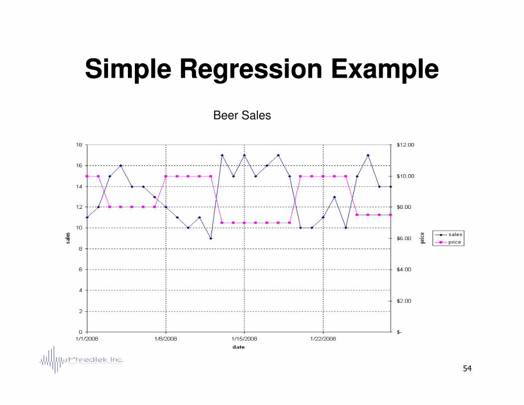
Simple Regression ExampleSimple Regression Example
Beer Sales
54
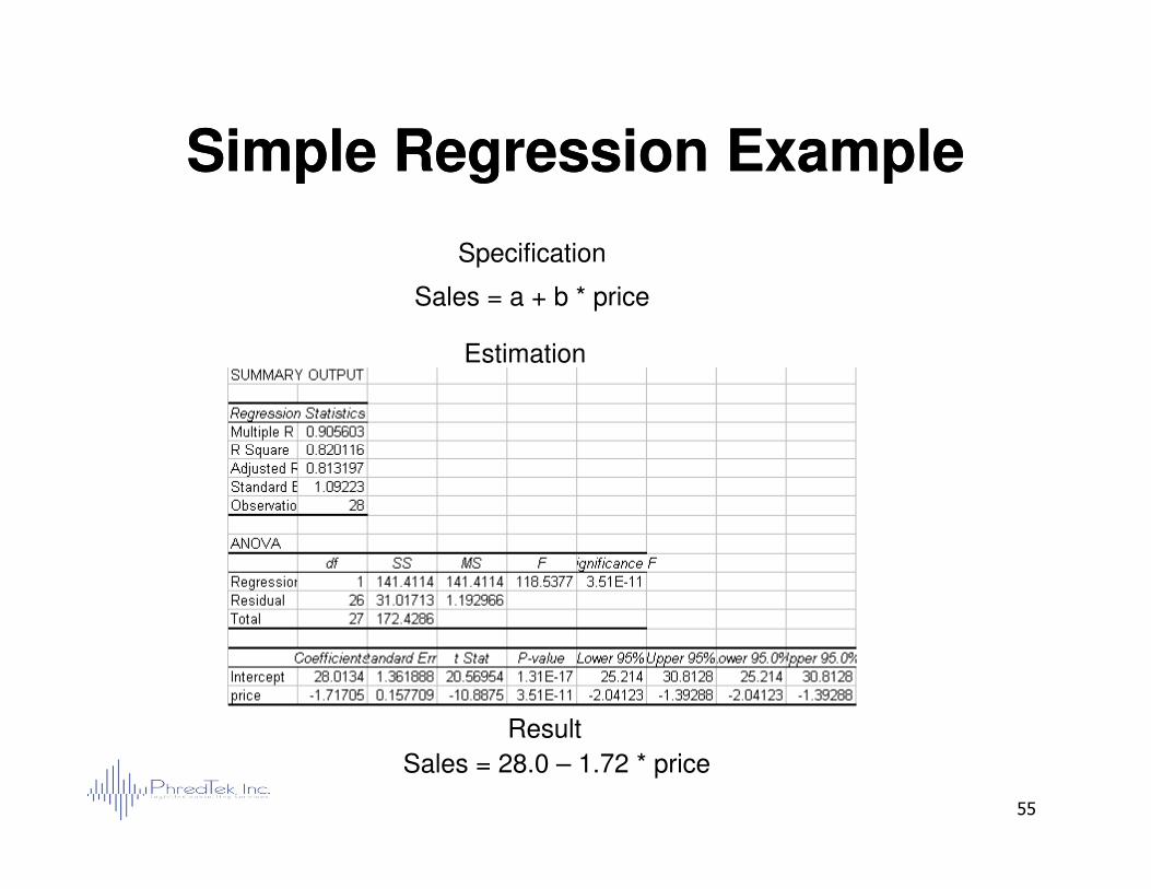
Simple Regression ExampleSimple Regression Example
Specification
Sales = a + b * price
Estimation
55
Result
Sales = 28.0 – 1.72 * price
•• T testT test
•• R squareR square
•• Standard Error of the residualsStandard Error of the residuals
Simple Regression ForecastingSimple Regression Forecasting3) Validation3) Validation
•• Standard Error of the residualsStandard Error of the residuals
•• Sign of the coefficientsSign of the coefficients
•• F testF test
•• AutocorrelationAutocorrelation
56
Simple Regression ForecastingSimple Regression Forecasting3) Validation 3) Validation -- T TestT Test
•• Tests whether or not the slope is really Tests whether or not the slope is really different from 0.different from 0.
•• T value is the ratio of the slope to its T value is the ratio of the slope to its standard deviation standard deviation –– that is, it is the that is, it is the
57
standard deviation standard deviation –– that is, it is the that is, it is the number of standard deviations away from number of standard deviations away from 0.0.
•• P value is the probability of getting that P value is the probability of getting that slope if the true slope is 0.slope if the true slope is 0.
•• Generally accepted “good” P value is .05 Generally accepted “good” P value is .05 or less.or less.
Simple Regression ForecastingSimple Regression Forecasting3) Validation 3) Validation -- R SquareR Square
•• Measures the fraction of the variability in the Measures the fraction of the variability in the dependent variable that is explained by the dependent variable that is explained by the independent variable.independent variable.
•• Ranges between 0 and 1Ranges between 0 and 1
–– 1 means all the variability is explained.1 means all the variability is explained.
58
–– 1 means all the variability is explained.1 means all the variability is explained.
–– 0 means none of the variability is explained.0 means none of the variability is explained.
•• Adjusted R square Adjusted R square –– an attempt by statisticians to an attempt by statisticians to purify the raw R square that I have never found useful.purify the raw R square that I have never found useful.
•• R squares > .9 are very good for forecasting.R squares > .9 are very good for forecasting.
•• However, R squares as low as .5 can still be useful.However, R squares as low as .5 can still be useful.
Simple Regression ForecastingSimple Regression Forecasting3) Validation 3) Validation ––
Standard Error of the ResidualsStandard Error of the Residuals
•• Gives a good estimate of future forecast Gives a good estimate of future forecast error.error.
•• Can be used to determine. confidence Can be used to determine. confidence
59
limits on the forecast.limits on the forecast.
•• Can be used to set safety stock.Can be used to set safety stock.
Simple Regression ForecastingSimple Regression Forecasting3) Validation 3) Validation -- F testF test
•• Tests whether both the slope and the Tests whether both the slope and the intercept are simultaneously greater than intercept are simultaneously greater than 0.0.
•• P value of .05 or less again is generally P value of .05 or less again is generally
60
•• P value of .05 or less again is generally P value of .05 or less again is generally accepted as significant.accepted as significant.
•• Passing the F test alone does not say the Passing the F test alone does not say the regression is useful.regression is useful.
•• I have never found this test useful.I have never found this test useful.
Simple Regression ForecastingSimple Regression Forecasting3) Validation 3) Validation -- AutocorrelationAutocorrelation
•• Autocorrelation results in a pattern in the Autocorrelation results in a pattern in the residuals.residuals.
•• Can be determined two ways:Can be determined two ways:–– Visually from a graph (easy)Visually from a graph (easy)
61
–– Visually from a graph (easy)Visually from a graph (easy)
–– A DurbinA Durbin--Watson statistic < 1.5 or > 2.5Watson statistic < 1.5 or > 2.5
•• Sometimes autocorrelation can be Sometimes autocorrelation can be corrected by adding variables (multiple corrected by adding variables (multiple regression)regression)
•• Most of the time, autocorrelation cannot be Most of the time, autocorrelation cannot be corrected without advanced techniques corrected without advanced techniques ––we will discuss this later.we will discuss this later.
Simple Regression ForecastingSimple Regression Forecasting4) Doing the Forecast4) Doing the Forecast
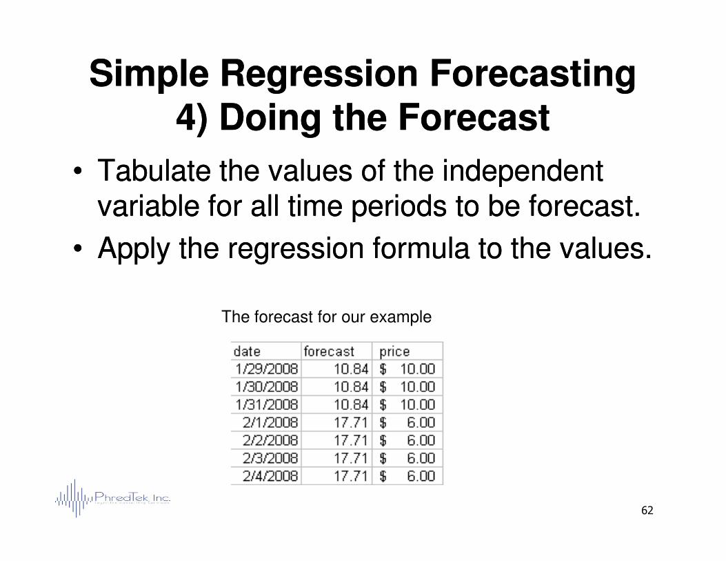
•• Tabulate the values of the independent Tabulate the values of the independent variable for all time periods to be forecast.variable for all time periods to be forecast.
•• Apply the regression formula to the values.Apply the regression formula to the values.
62
The forecast for our example
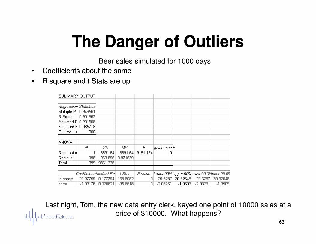
The Danger of OutliersThe Danger of Outliers
•• Coefficients about the sameCoefficients about the same
•• R square and t Stats are up.R square and t Stats are up.
Beer sales simulated for 1000 days
63
Last night, Tom, the new data entry clerk, keyed one point of 10000 sales at a price of $10000. What happens?
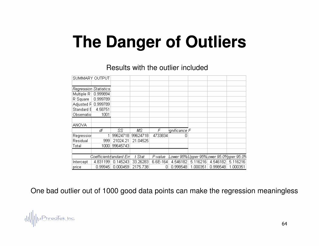
The Danger of OutliersThe Danger of Outliers
Results with the outlier included
64
One bad outlier out of 1000 good data points can make the regression meaningless
Multiple Regression Multiple Regression ForecastingForecasting
•• Same as simple, but more than one variable.Same as simple, but more than one variable.
•• Y = Bt + e where:Y = Bt + e where:
–– Y is a column of numbers (vector) which are the Y is a column of numbers (vector) which are the values of the dependent variable.values of the dependent variable.
65
–– B is a matrix where the first column is all ones and B is a matrix where the first column is all ones and each successive column contains the valued of the each successive column contains the valued of the independent variables.independent variables.
–– t is a column of numbers which are the coefficients to t is a column of numbers which are the coefficients to be estimated.be estimated.
–– e is a column of numbers which are the error.e is a column of numbers which are the error.
•• Y and B are known. t and e are to be estimated.Y and B are known. t and e are to be estimated.
Multiple Regression Multiple Regression ForecastingForecasting
•• Steps are the same as simple regression.Steps are the same as simple regression.
•• Having a business reason for why each Having a business reason for why each independent variable effects the independent variable effects the dependent variable is more important.dependent variable is more important.
66
dependent variable is more important.dependent variable is more important.
•• Most all software packages that do simple Most all software packages that do simple regression also do multiple regression.regression also do multiple regression.
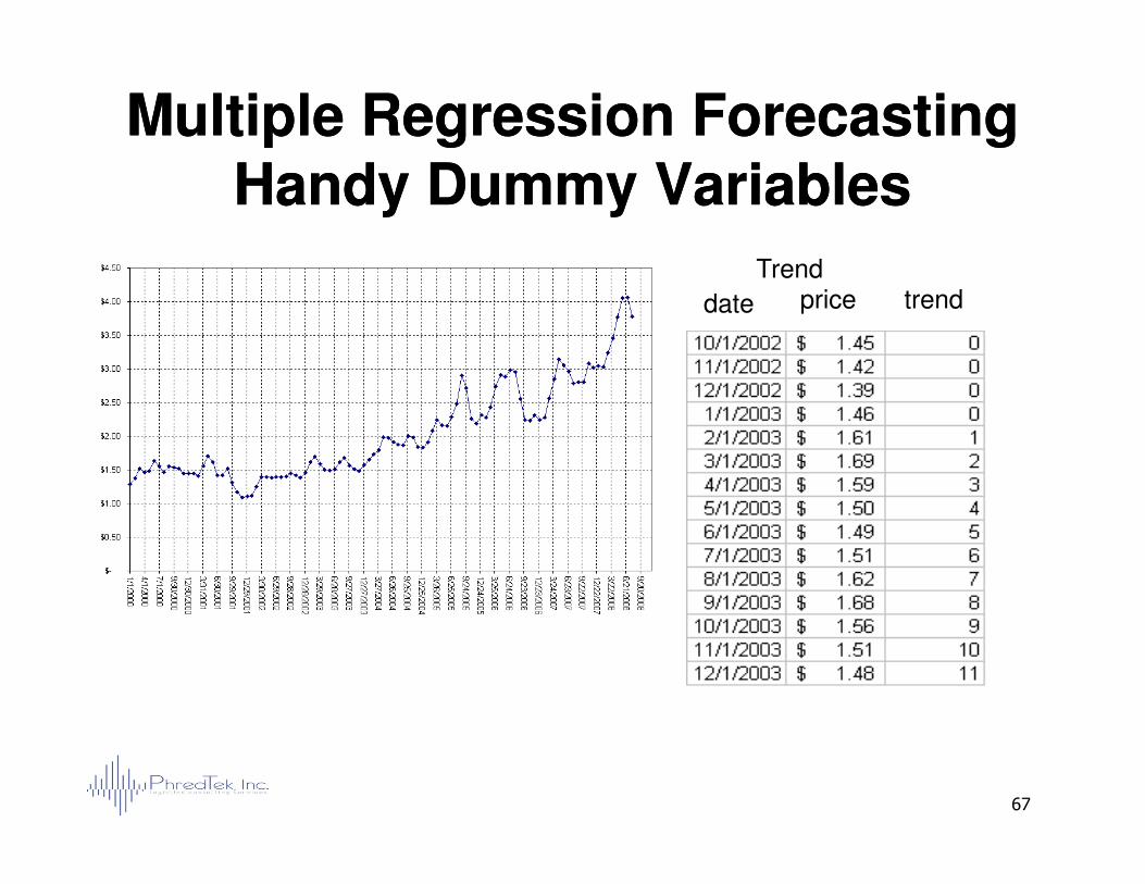
Multiple Regression ForecastingMultiple Regression ForecastingHandy Dummy VariablesHandy Dummy Variables
Trend
date price trend
67
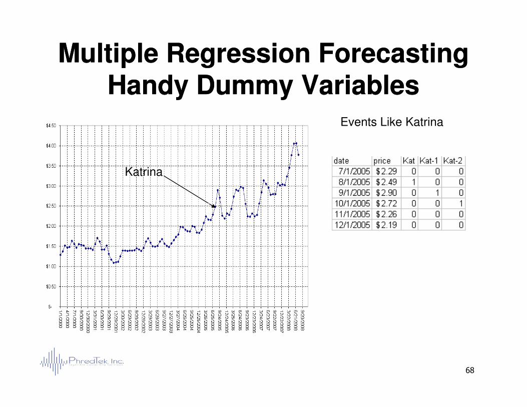
Multiple Regression ForecastingMultiple Regression ForecastingHandy Dummy VariablesHandy Dummy Variables
Events Like Katrina
Katrina
68
Multiple Regression ForecastingMultiple Regression ForecastingNew ProblemNew Problem
•• Two or more independent variables can be Two or more independent variables can be related to one another related to one another –– called multicollinearity.called multicollinearity.
•• Example Example –– the population of a town and the the population of a town and the number of churches in it.number of churches in it.
69
number of churches in it.number of churches in it.
•• Keeping both in the model causes bad Keeping both in the model causes bad coefficient estimates for both.coefficient estimates for both.
•• Use business based reasoning to determine Use business based reasoning to determine which is the true causal variable.which is the true causal variable.
•• If the correlation is exactly one, a good If the correlation is exactly one, a good regression package will drop one of them.regression package will drop one of them.
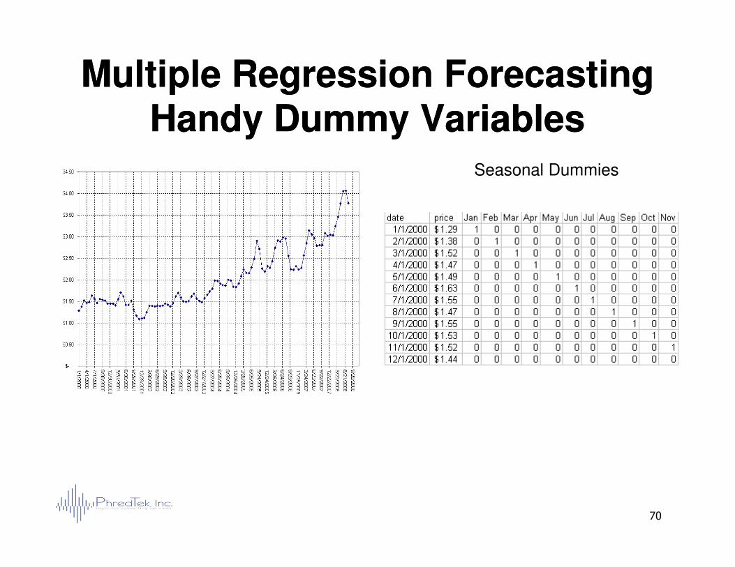
Multiple Regression ForecastingMultiple Regression ForecastingHandy Dummy VariablesHandy Dummy Variables
Seasonal Dummies
70
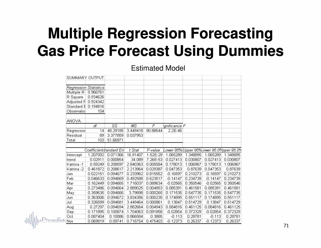
Multiple Regression ForecastingMultiple Regression ForecastingGas Price Forecast Using DummiesGas Price Forecast Using Dummies
Estimated Model
71
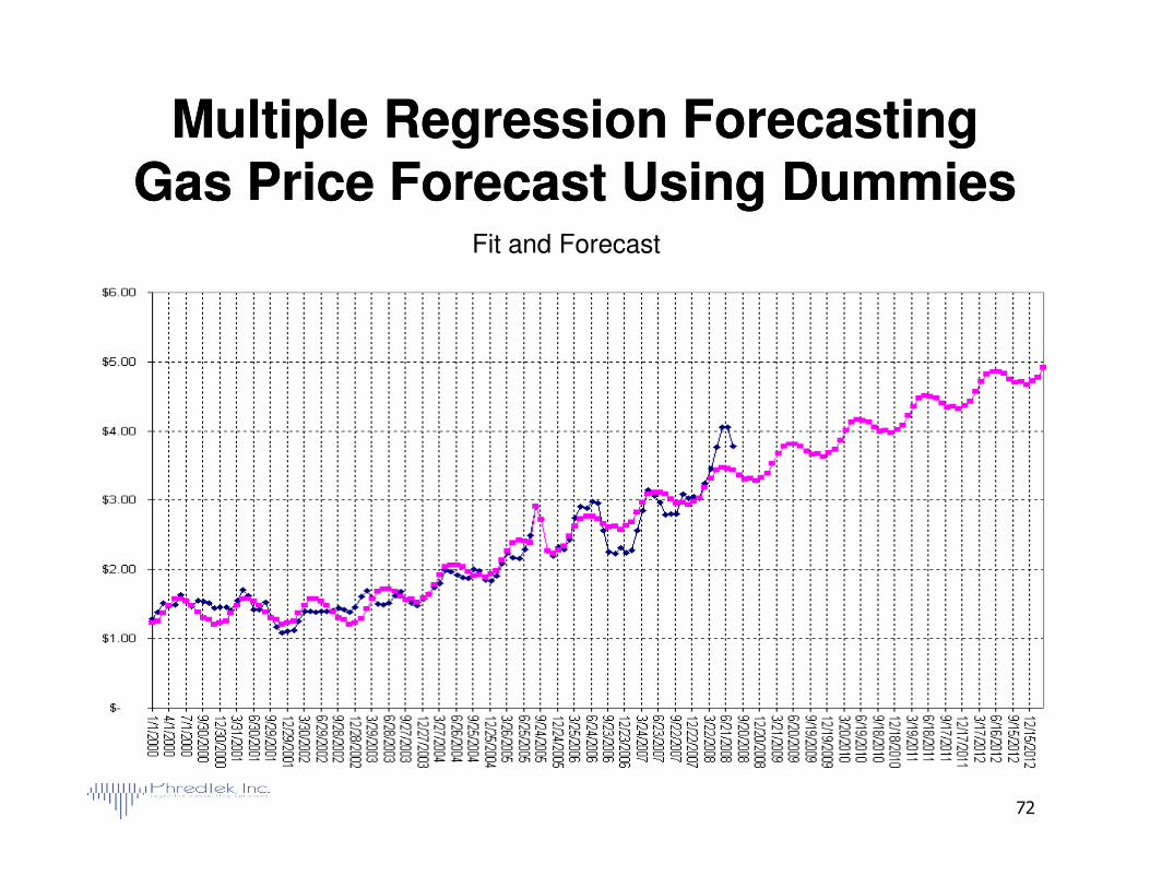
Multiple Regression ForecastingMultiple Regression ForecastingGas Price Forecast Using DummiesGas Price Forecast Using Dummies
Fit and Forecast
72
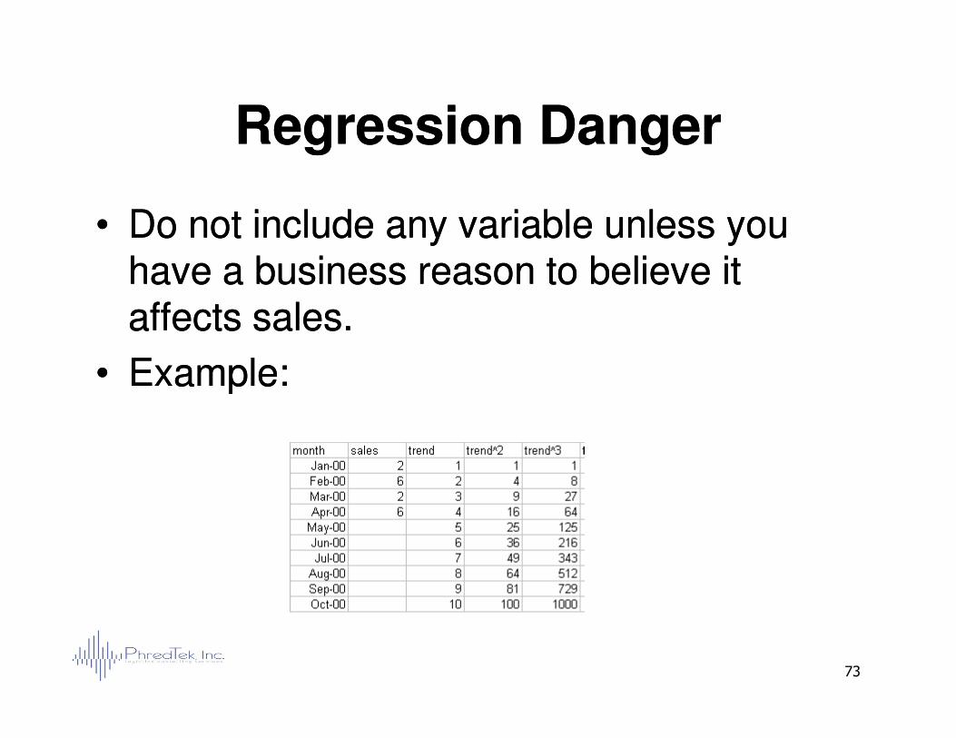
Regression DangerRegression Danger
•• Do not include any variable unless you Do not include any variable unless you have a business reason to believe it have a business reason to believe it affects sales.affects sales.
•• Example:Example:
73
•• Example:Example:
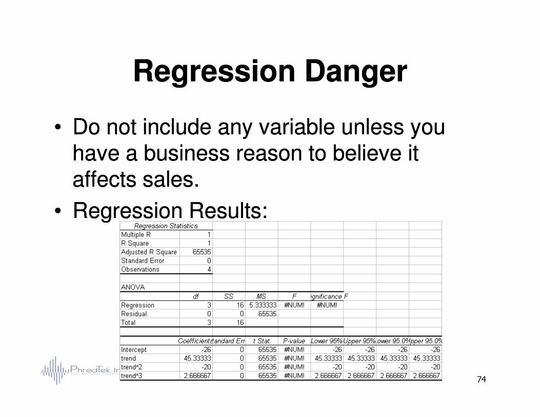
Regression DangerRegression Danger
•• Do not include any variable unless you Do not include any variable unless you have a business reason to believe it have a business reason to believe it affects sales.affects sales.
•• Regression Results:Regression Results:
74
•• Regression Results:Regression Results:
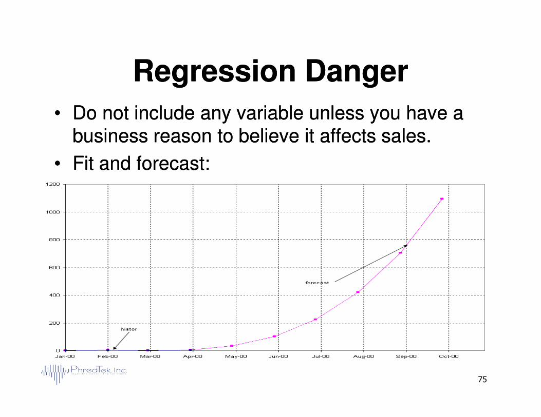
Regression DangerRegression Danger
•• Do not include any variable unless you have a Do not include any variable unless you have a business reason to believe it affects sales.business reason to believe it affects sales.
•• Fit and forecast:Fit and forecast:
75
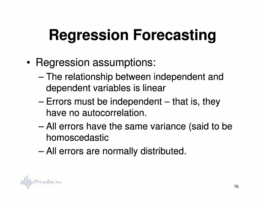
Regression ForecastingRegression Forecasting
•• Regression assumptions:Regression assumptions:
–– The relationship between independent and The relationship between independent and dependent variables is lineardependent variables is linear
–– Errors must be independent Errors must be independent –– that is, they that is, they
76
–– Errors must be independent Errors must be independent –– that is, they that is, they have no have no autocorrelation.autocorrelation.
–– All errors have the same variance (said to be All errors have the same variance (said to be homoscedastichomoscedastic
–– All errors are normally distributed.All errors are normally distributed.

Excel ExerciseExcel ExerciseExcel ExerciseExcel Exercise
4. Forecasting 4. Forecasting AccuracyAccuracyAccuracyAccuracy
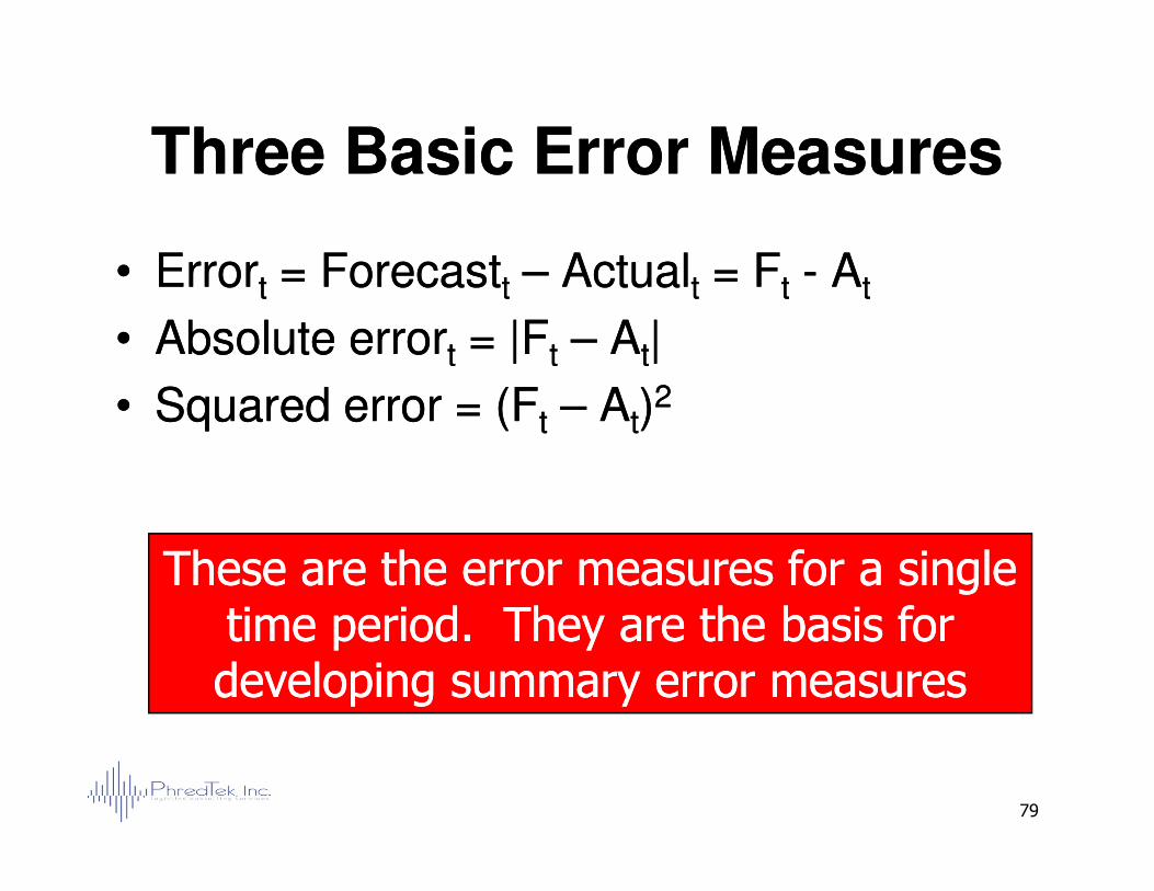
Three Basic Error MeasuresThree Basic Error Measures
•• ErrorErrortt = Forecast= Forecasttt –– ActualActualtt = F= Ftt -- AAtt
•• Absolute errorAbsolute errortt = |F= |Ftt –– AAtt||
•• Squared error = (FSquared error = (Ftt –– AAtt))22
79
These are the error measures for a single These are the error measures for a single time period. They are the basis for time period. They are the basis for developing summary error measuresdeveloping summary error measures
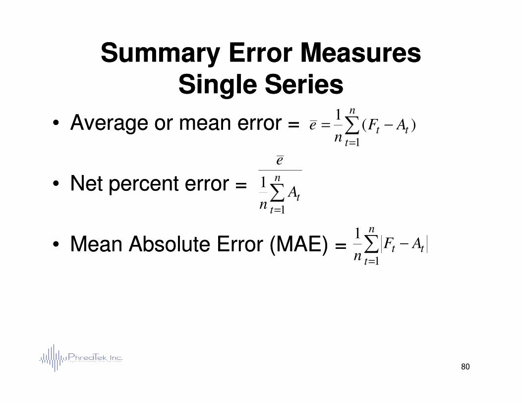
Summary Error MeasuresSummary Error MeasuresSingle SeriesSingle Series
•• Average or mean error =Average or mean error =
•• Net percent error =Net percent error =
∑=
−=
n
ttt AF
ne
1
)(1
∑=
n
tAn
e
1
80
•• Mean Absolute Error (MAE) =Mean Absolute Error (MAE) = ∑=
−
n
ttt AF
n 1
1
∑=t
tn 1
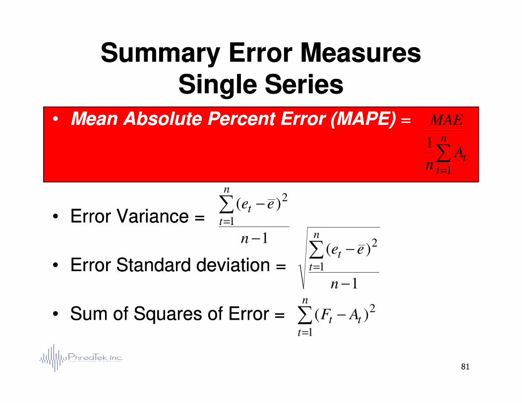
Summary Error MeasuresSummary Error MeasuresSingle SeriesSingle Series
•• Mean Absolute Percent Error (MAPE)Mean Absolute Percent Error (MAPE) ==
)( 2−∑ ee
n
t
∑=
n
ttA
n
MAE
1
1
81
•• Error Variance =Error Variance =
•• Error Standard deviation =Error Standard deviation =
•• Sum of Squares of Error = Sum of Squares of Error =
1
)(1
2
−
−∑=
n
eet
t
1
)(1
2
−
−∑=
n
een
tt
∑=
−
n
ttt AF
1
2)(
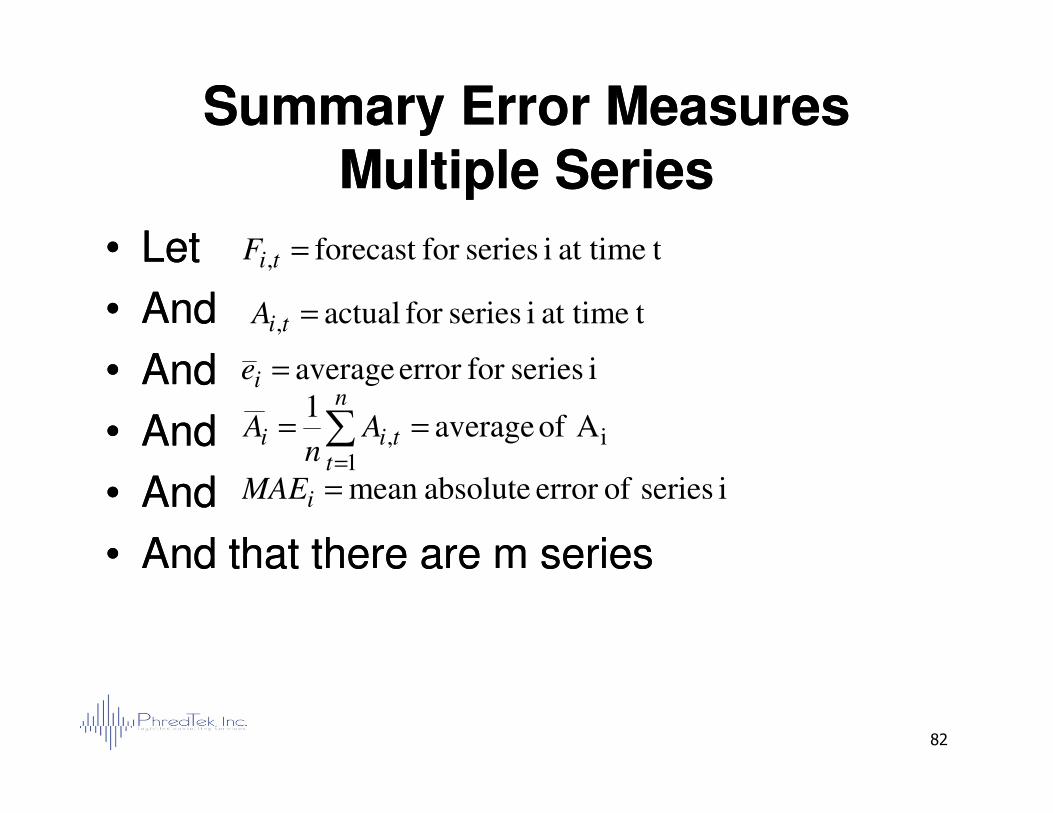
Summary Error MeasuresSummary Error MeasuresMultiple SeriesMultiple Series
•• LetLet
•• AndAnd
•• AndAnd
•• AndAnd
tat time i seriesfor forecast , =tiF
tat time i seriesfor actual , =tiA
i seriesfor error average =ie
1== ∑
n
82
•• AndAnd
•• AndAnd
•• And that there are m seriesAnd that there are m series
i1
, A of average 1
== ∑=
n
ttii A
nA
i series oferror absolutemean =iMAE
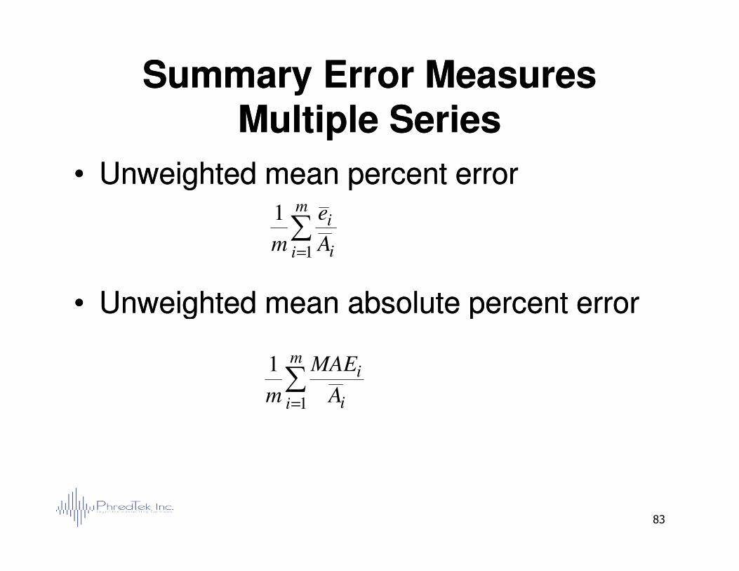
Summary Error MeasuresSummary Error MeasuresMultiple SeriesMultiple Series
•• Unweighted mean percent errorUnweighted mean percent error
•• Unweighted mean absolute percent errorUnweighted mean absolute percent error
∑=
m
i i
i
A
e
m 1
1
83
•• Unweighted mean absolute percent errorUnweighted mean absolute percent error
∑=
m
i i
i
A
MAE
m 1
1
Summary Error MeasuresSummary Error MeasuresMultiple SeriesMultiple Series
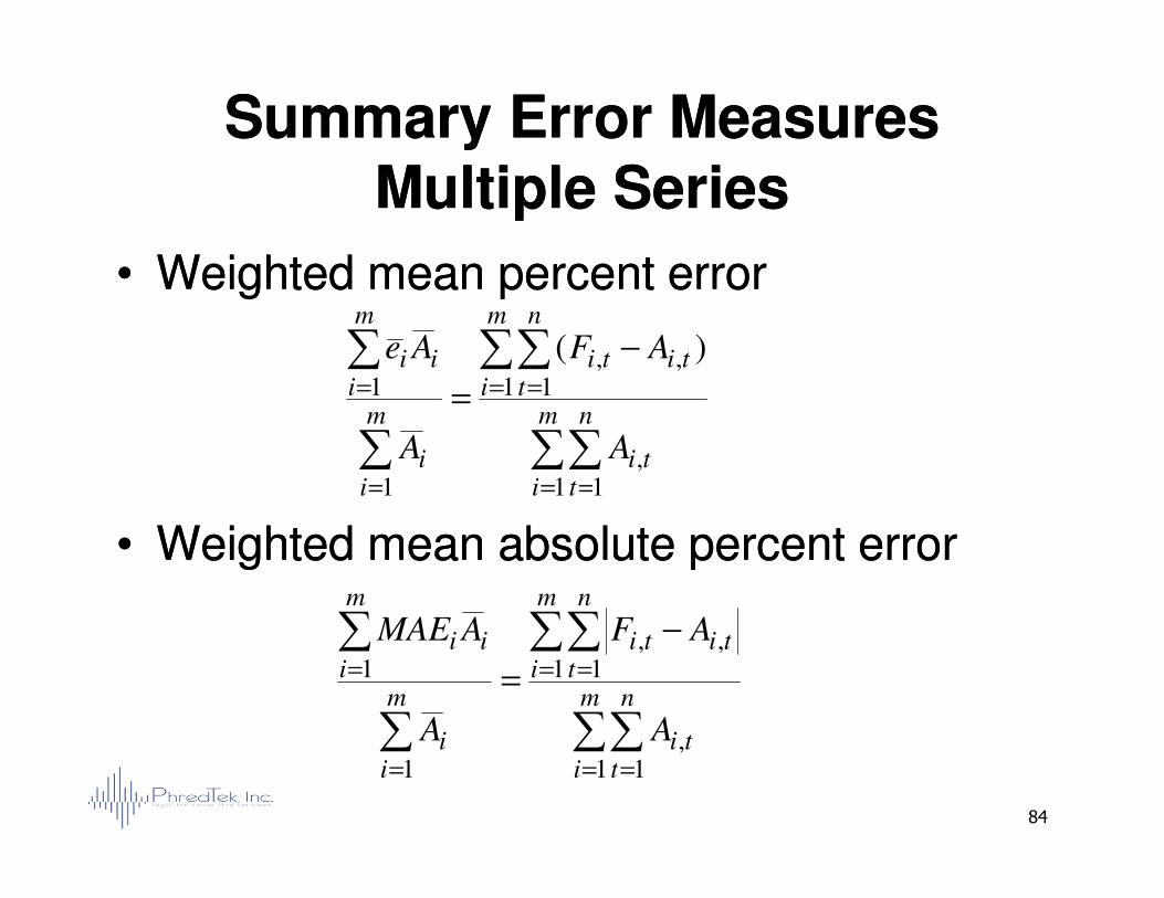
•• Weighted mean percent errorWeighted mean percent error
∑∑
∑∑
∑
∑= ==
−
=m n
ti
m
i
n
ttiti
m
i
m
iii
A
AF
A
Ae
,
1 1,,
1
)(
84
•• Weighted mean absolute percent errorWeighted mean absolute percent error
∑∑∑= == i t
tii
i AA1 1
,1
∑∑
∑∑
∑
∑
= =
= =
=
=
−
=m
i
n
tti
m
i
n
ttiti
m
ii
m
iii
A
AF
A
AMAE
1 1,
1 1,,
1
1
Uses of Summary Error MeasuresUses of Summary Error MeasuresSingle SeriesSingle Series
•• Average or mean error Average or mean error –– describes the bias of the describes the bias of the forecast. It should go to zero over time or the forecast forecast. It should go to zero over time or the forecast needs improvement.needs improvement.
•• Net percent error Net percent error –– describes the bias relative to average describes the bias relative to average sales sales –– most useful for communication to othersmost useful for communication to others
85
sales sales –– most useful for communication to othersmost useful for communication to others
•• Mean absolute error Mean absolute error –– describes the pain the forecast describes the pain the forecast will inflict because over forecasts are generally just as will inflict because over forecasts are generally just as bad or worse than under forecasts.bad or worse than under forecasts.
•• Mean absolute percent error (MAPE) Mean absolute percent error (MAPE) –– most useful most useful statistic for communicating forecast error to others.statistic for communicating forecast error to others.
Uses of Summary Error MeasuresUses of Summary Error MeasuresSingle SeriesSingle Series
•• Error variance and standard deviation are used Error variance and standard deviation are used for determining confidence limits of forecasts for determining confidence limits of forecasts and for setting safety stock.and for setting safety stock.
•• Sum of squared error is the most common Sum of squared error is the most common
86
•• Sum of squared error is the most common Sum of squared error is the most common statistic that is minimized to fit a forecast model. statistic that is minimized to fit a forecast model. It is also useful for comparing one model fit to It is also useful for comparing one model fit to another.another.
Uses of Uses of Summary Error Summary Error MeasuresMeasuresMultiple Multiple SeriesSeries
•• Mean percent error and mean absolute percent Mean percent error and mean absolute percent error have the same use for multiple series as error have the same use for multiple series as they to for a single series.they to for a single series.
•• Use weighted when the units of measure for all Use weighted when the units of measure for all
87
•• Use weighted when the units of measure for all Use weighted when the units of measure for all series are the same.series are the same.
•• Use unweighted when the units of measure are Use unweighted when the units of measure are different.different.
Save All Your ForecastsSave All Your Forecasts•• Data storage is inexpensive.Data storage is inexpensive.
•• Database Database should contain:should contain:
–– Forecast origin Forecast origin –– last date in history used to generate the last date in history used to generate the forecastforecast
–– Forecast date Forecast date –– the date being forecastthe date being forecast
88
–– Forecast valueForecast value
–– Actual sales for the forecast date once it is available.Actual sales for the forecast date once it is available.
•• For example if you do a 26 week forecast, you will have For example if you do a 26 week forecast, you will have 26 forecasts for each week.26 forecasts for each week.
•• You can now evaluate any forecast error and:You can now evaluate any forecast error and:
–– Clearly demonstrate improvement over timeClearly demonstrate improvement over time
–– Identify those forecasts in need of improvementIdentify those forecasts in need of improvement
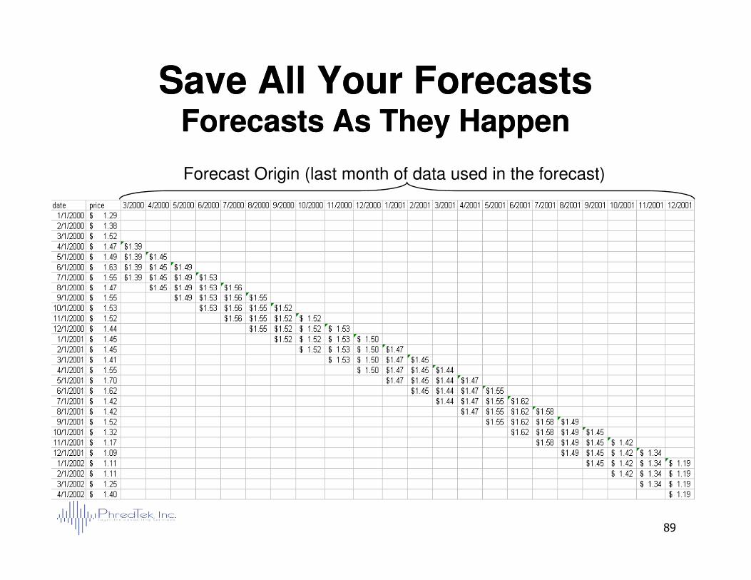
Save All Your ForecastsSave All Your ForecastsForecasts As They HappenForecasts As They Happen
Forecast Origin (last month of data used in the forecast)
89
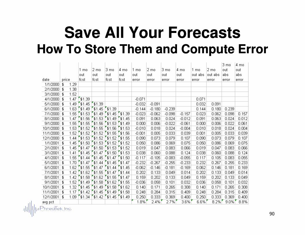
Save All Your ForecastsSave All Your ForecastsHow To Store Them and Compute ErrorHow To Store Them and Compute Error
90
Improving Forecast AccuracyImproving Forecast Accuracy
•• Regularly review forecast errorRegularly review forecast error
•• Rank from largest to smallest mean Rank from largest to smallest mean absolute error.absolute error.
•• Graph the errors and look for patternsGraph the errors and look for patterns
91
•• Graph the errors and look for patternsGraph the errors and look for patterns
•• When you see a pattern, think about what When you see a pattern, think about what business driver caused it.business driver caused it.
•• When you find a new business driver, When you find a new business driver, factor it into the forecast.factor it into the forecast.
Improving Forecast AccuracyImproving Forecast Accuracy
•• Assign responsibility and accountability for Assign responsibility and accountability for forecasts (across all stakeholder groups)forecasts (across all stakeholder groups)
•• Set realistic goals error reduction.Set realistic goals error reduction.
•• Tie performance reviews to goalsTie performance reviews to goals
92
•• Tie performance reviews to goalsTie performance reviews to goals
•• Provide good forecasting toolsProvide good forecasting tools
Goodness of Fit vs. Forecasting Goodness of Fit vs. Forecasting AccuracyAccuracy
•• Two methods of choosing forecasting Two methods of choosing forecasting method:method:–– Forecast Accuracy Forecast Accuracy -- Withhold the last several Withhold the last several
historic values of actual sales, build a forecast historic values of actual sales, build a forecast based on the rest. Choose the method which based on the rest. Choose the method which
93
based on the rest. Choose the method which based on the rest. Choose the method which best forecasts the withheld values.best forecasts the withheld values.
–– Goodness of Fit Goodness of Fit -- Choose the method which Choose the method which best fits all the historical values. That is, the best fits all the historical values. That is, the method which minimizes the sum of squares method which minimizes the sum of squares of the fit minus the actual. of the fit minus the actual.
Forecasting Accuracy vs. Forecasting Accuracy vs. Goodness of FitGoodness of Fit
•• Two methods of choosing forecasting method:Two methods of choosing forecasting method:
–– Forecast Accuracy Forecast Accuracy –– Withhold the last several historic Withhold the last several historic values of actual sales, build a forecast based on the values of actual sales, build a forecast based on the rest. Choose the method which best forecasts the rest. Choose the method which best forecasts the withheld values using.withheld values using.
94
withheld values using.withheld values using.
–– Goodness of Fit Goodness of Fit -- Choose the method which best Choose the method which best characterizes the historical values using pattern characterizes the historical values using pattern recognition and business knowledge of the process. recognition and business knowledge of the process. Perform accepted model identification and model Perform accepted model identification and model revision using statistical modeling procedures.revision using statistical modeling procedures.
Fitting versus ModelingFitting versus Modeling
•• Two methods of choosing forecasting method:Two methods of choosing forecasting method:
–– Forecast Accuracy Forecast Accuracy –– Older Classical method based Older Classical method based on using a list of models and simply picking the best on using a list of models and simply picking the best of the list. No guarantees about statistical of the list. No guarantees about statistical methodologies simply a sequence of trial models. methodologies simply a sequence of trial models.
95
methodologies simply a sequence of trial models. methodologies simply a sequence of trial models. Does not incorporate any knowledge of the business Does not incorporate any knowledge of the business process.process.
–– Goodness of Fit Goodness of Fit –– Choose variables that are known to Choose variables that are known to affect sales. Iterate to the best model set of affect sales. Iterate to the best model set of parameters by performing formal statistical tests.parameters by performing formal statistical tests.
Modeling WinsModeling Wins
•• Fitting to minimize forecast error method is like the tail wagging the Fitting to minimize forecast error method is like the tail wagging the dog.dog.–– The answer is very different depending on how many observations are The answer is very different depending on how many observations are
withheld.withheld.–– The method chosen can change with each forecast run The method chosen can change with each forecast run –– leads to leads to
unstable forecasts and generally higher real forecast error.unstable forecasts and generally higher real forecast error.–– No statistical tests are conducted for Necessity or SufficiencyNo statistical tests are conducted for Necessity or Sufficiency–– They are not based on solid business based cause and effect They are not based on solid business based cause and effect
96
–– They are not based on solid business based cause and effect They are not based on solid business based cause and effect relationships.relationships.
•• ModellingModelling–– Is stable because only statistically significant coefficients are used and Is stable because only statistically significant coefficients are used and
the error process of the model is white noise (random) the error process of the model is white noise (random) –– Makes the management decision process more stable as model Makes the management decision process more stable as model
forms/parameters are less volatile forms/parameters are less volatile –– Makes the forecast more credible as equations have rational structure Makes the forecast more credible as equations have rational structure
and can be easily explained to nonand can be easily explained to non--quantitative associates quantitative associates –– Allows systematic forecast improvement.Allows systematic forecast improvement.
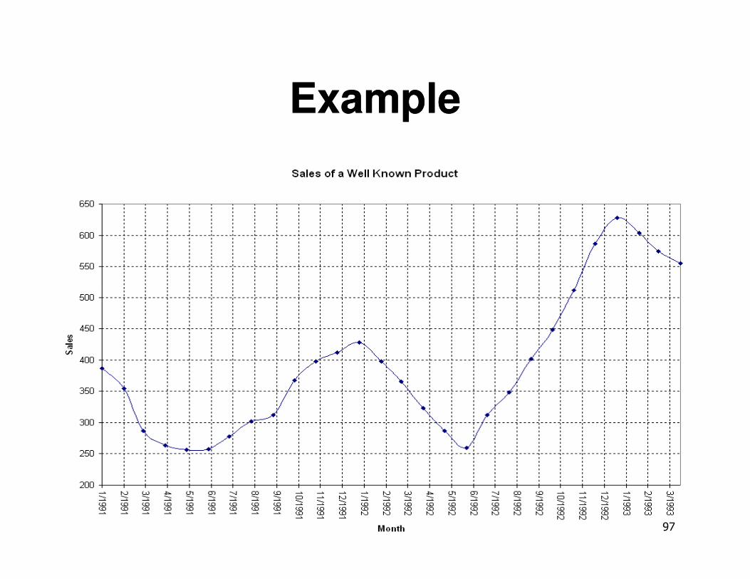
ExampleExample
97
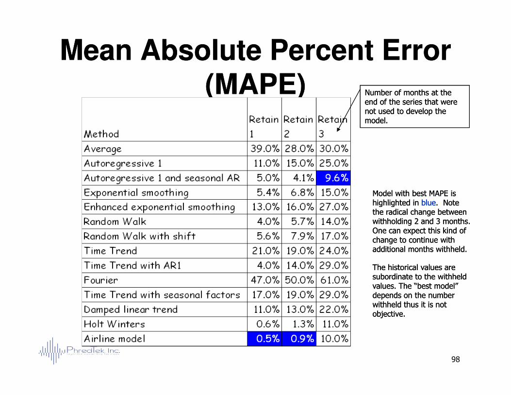
Mean Absolute Percent Error Mean Absolute Percent Error (MAPE)(MAPE) Number of months at the Number of months at the
end of the series that were end of the series that were not used to develop the not used to develop the model. model.
Model with best MAPE is Model with best MAPE is highlighted in highlighted in blueblue. Note . Note
98
highlighted in highlighted in blueblue. Note . Note the radical change between the radical change between withholding 2 and 3 months. withholding 2 and 3 months. One can expect this kind of One can expect this kind of change to continue with change to continue with additional months withheld.additional months withheld.
The historical values are The historical values are subordinate to the withheld subordinate to the withheld values. The “best model” values. The “best model” depends on the number depends on the number withheld thus it is not withheld thus it is not objective.objective.
Using Forecast Error to Using Forecast Error to Determine Safety StockDetermine Safety Stock
•• Compute the standard deviation of the forecast errorCompute the standard deviation of the forecast error–– It’s best if you have actual historical forecast error.It’s best if you have actual historical forecast error.–– If not, the standard deviation of the fit will sufficeIf not, the standard deviation of the fit will suffice
•• Determine the acceptable chances of a stock out. This is dependent Determine the acceptable chances of a stock out. This is dependent on two factorson two factors–– Inventory holding cost. The higher the holding cost, the higher chances Inventory holding cost. The higher the holding cost, the higher chances
of stock outs you are willing to accept.of stock outs you are willing to accept.
99
of stock outs you are willing to accept.of stock outs you are willing to accept.–– Stock out cost. Generally, this is lost sales. The higher the stock out Stock out cost. Generally, this is lost sales. The higher the stock out
costs, the lower you want the chances of stocking out.costs, the lower you want the chances of stocking out.–– Inventory holding costs are easy to compute, but stock out costs often Inventory holding costs are easy to compute, but stock out costs often
require an expensive market research study to determine. Therefore, require an expensive market research study to determine. Therefore, an intuitive guess based on your business knowledge is generally an intuitive guess based on your business knowledge is generally sufficient.sufficient.
•• Look the stock out probability up in a normal table to determine the Look the stock out probability up in a normal table to determine the number of standard deviations necessary to achieve it.number of standard deviations necessary to achieve it.
•• Multiply that number by the standard deviation of forecast error Multiply that number by the standard deviation of forecast error
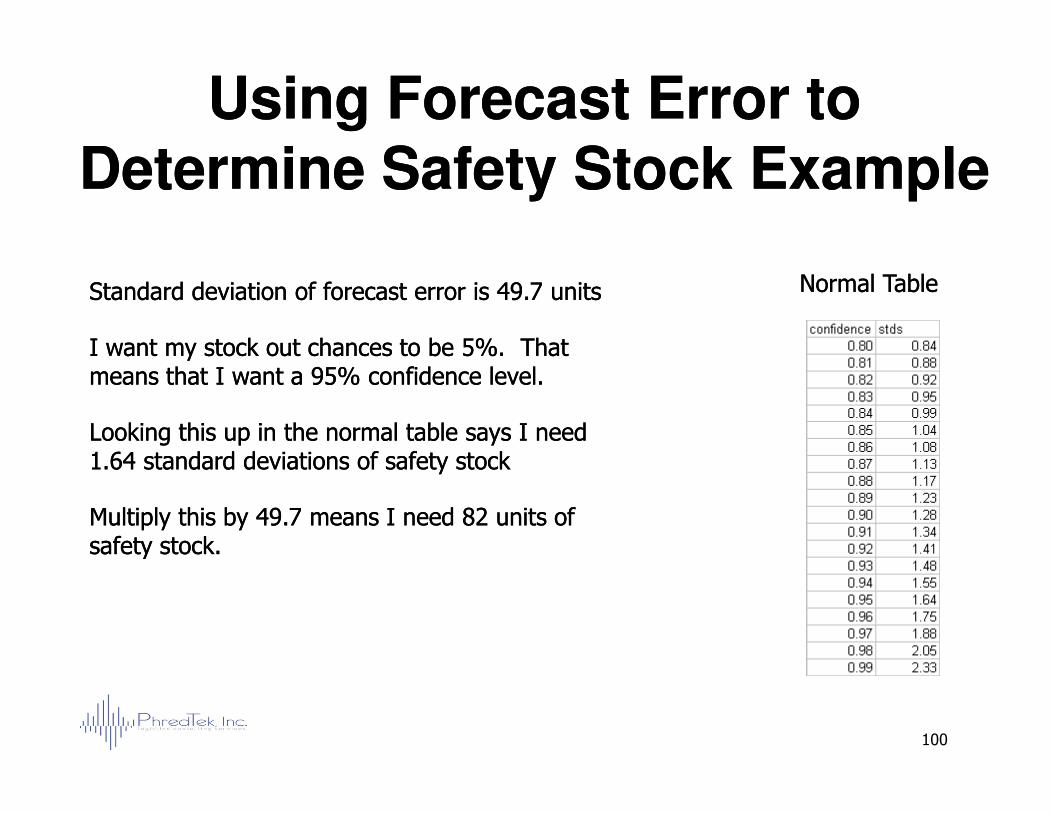
Using Forecast Error to Using Forecast Error to Determine Safety Stock ExampleDetermine Safety Stock Example
Normal TableNormal TableStandard deviation of forecast error is 49.7 unitsStandard deviation of forecast error is 49.7 units
I want my stock out chances to be 5%. That I want my stock out chances to be 5%. That means that I want a 95% confidence level.means that I want a 95% confidence level.
100
Looking this up in the normal table says I need Looking this up in the normal table says I need 1.64 standard deviations of safety stock1.64 standard deviations of safety stock
Multiply this by 49.7 means I need 82 units of Multiply this by 49.7 means I need 82 units of safety stock.safety stock.

5. Putting it all Together5. Putting it all TogetherThe Forecast ProcessThe Forecast ProcessThe Forecast ProcessThe Forecast Process
Building a Forecast ProcessBuilding a Forecast Process
•• Components of a forecast processComponents of a forecast process
–– PeoplePeople
–– SystemsSystems
–– Scheduled ActionsScheduled Actions
102
–– Scheduled ActionsScheduled Actions
–– Scheduled CommunicationsScheduled Communications
A forecast without a process to implement it will never be used.
Building a Forecast ProcessBuilding a Forecast Process
•• Necessary scheduled actionsNecessary scheduled actions
–– Collect dataCollect data
–– Generate forecastGenerate forecast
–– Save the forecastSave the forecast
103
–– Save the forecastSave the forecast
–– Tabulate forecast errorTabulate forecast error
•• Necessary scheduled communicationsNecessary scheduled communications
–– Communicate forecast to stakeholdersCommunicate forecast to stakeholders
–– Communicate error to stakeholdersCommunicate error to stakeholders
Building a Forecast ProcessBuilding a Forecast Process
•• Identify stakeholders Identify stakeholders –– People who People who allocate resources.allocate resources.–– SalesSales
–– MarketingMarketing
–– Supply Chain PlanningSupply Chain Planning
104
–– Supply Chain PlanningSupply Chain Planning
–– OperationsOperations
–– PurchasingPurchasing
–– Corporate PlanningCorporate Planning
–– EngineeringEngineering
–– DistributorsDistributors
–– RetailersRetailers
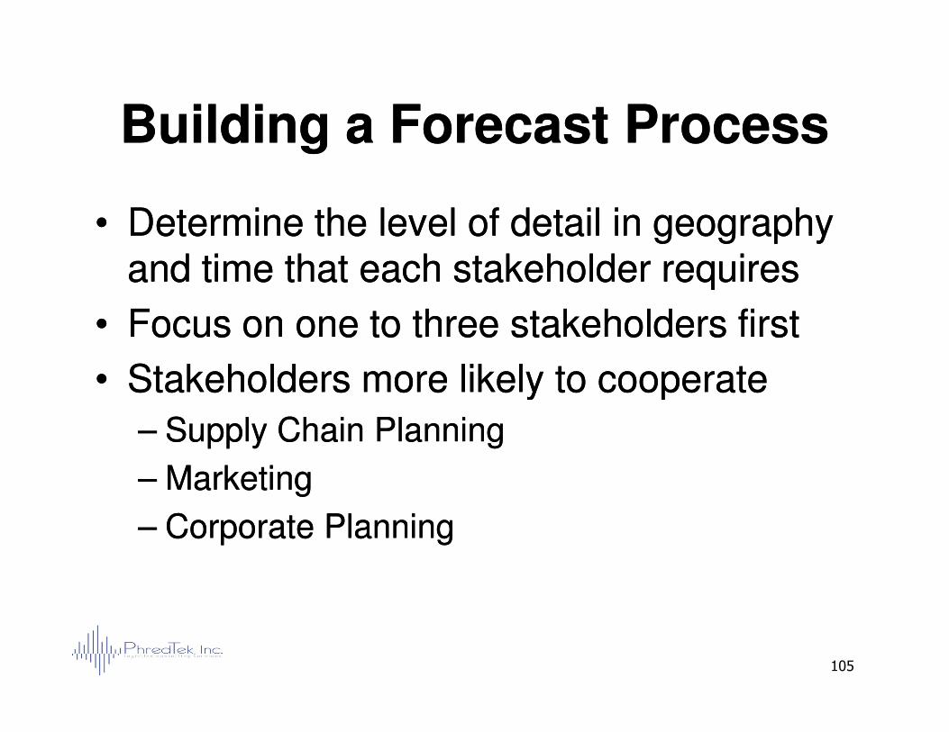
Building a Forecast ProcessBuilding a Forecast Process
•• Determine the level of detail in geography Determine the level of detail in geography and time that each stakeholder requiresand time that each stakeholder requires
•• Focus on one to three stakeholders firstFocus on one to three stakeholders first
•• Stakeholders more likely to cooperateStakeholders more likely to cooperate
105
•• Stakeholders more likely to cooperateStakeholders more likely to cooperate
–– Supply Chain PlanningSupply Chain Planning
–– MarketingMarketing
–– Corporate PlanningCorporate Planning
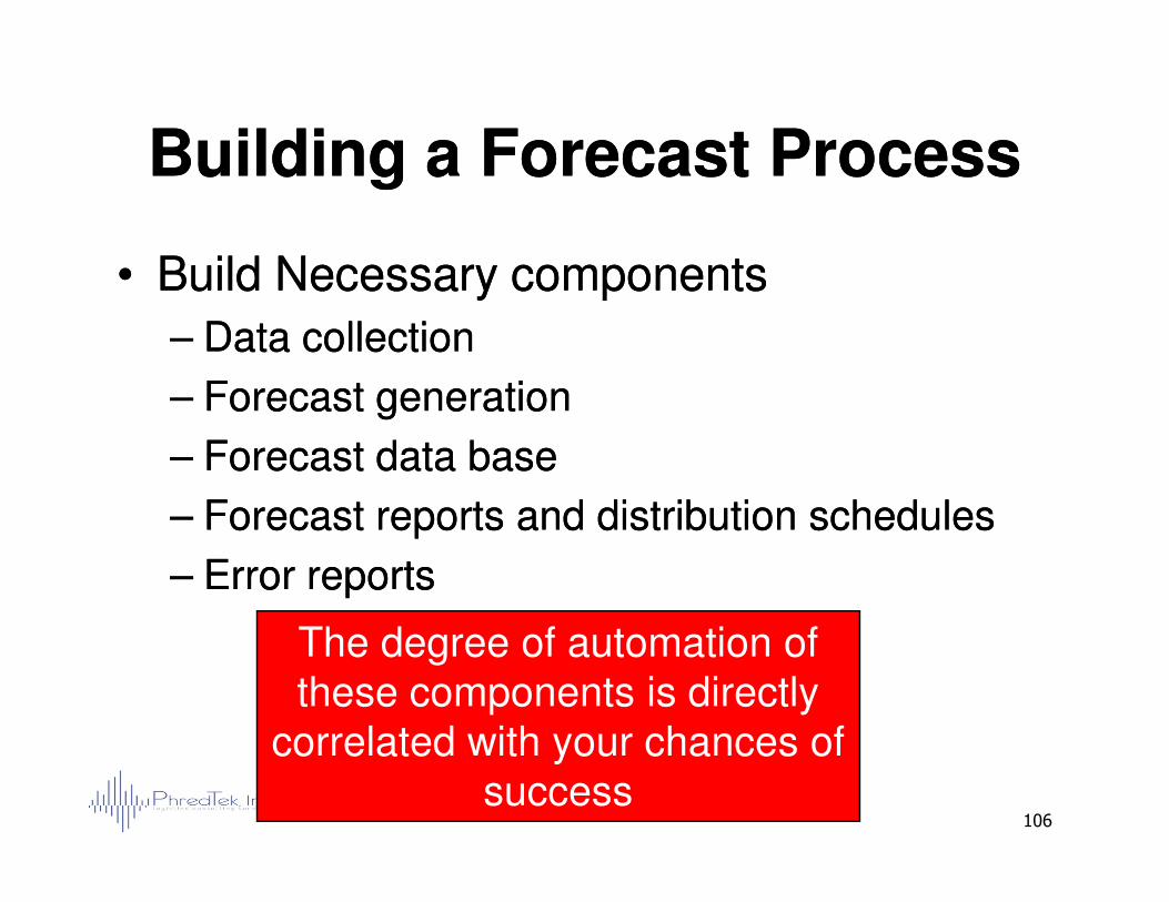
Building a Forecast ProcessBuilding a Forecast Process
•• Build Necessary componentsBuild Necessary components
–– Data collectionData collection
–– Forecast generationForecast generation
–– Forecast data baseForecast data base
106
–– Forecast data baseForecast data base
–– Forecast reports and distribution schedulesForecast reports and distribution schedules
–– Error reportsError reports
The degree of automation of these components is directly
correlated with your chances of success
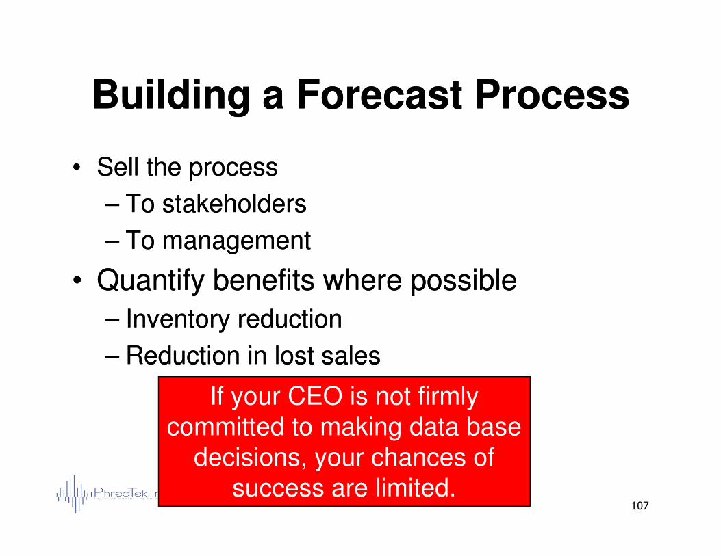
Building a Forecast ProcessBuilding a Forecast Process
•• Sell the processSell the process
–– To stakeholdersTo stakeholders
–– To managementTo management
•• Quantify benefits where possibleQuantify benefits where possible
107
•• Quantify benefits where possibleQuantify benefits where possible
–– Inventory reductionInventory reduction
–– Reduction in lost sales Reduction in lost sales
If your CEO is not firmly committed to making data base
decisions, your chances of success are limited.
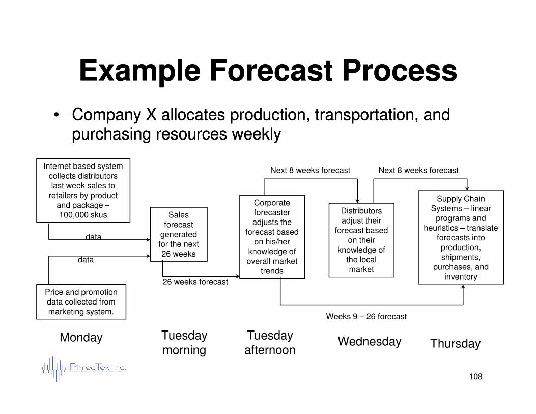
Example Forecast ProcessExample Forecast Process
•• Company X allocates production, transportation, and Company X allocates production, transportation, and purchasing resources weekly purchasing resources weekly
Internet based system collects distributors last week sales to
retailers by product and package – Corporate
Distributors
Supply Chain Systems – linear
Next 8 weeks forecast Next 8 weeks forecast
108
and package –100,000 skus
Price and promotion data collected from marketing system.
Sales forecast
generated for the next 26 weeks
forecaster adjusts the
forecast based on his/her
knowledge of overall market
trends
Distributors adjust their
forecast based on their
knowledge of the local market
Systems – linear programs and
heuristics – translate forecasts into production, shipments,
purchases, and inventory
data
data
26 weeks forecast
Weeks 9 – 26 forecast
Monday Tuesday morning
Tuesday afternoon
Wednesday Thursday
Software SelectionSoftware Selection
•• Software is required for a practical forecasting process.Software is required for a practical forecasting process.
•• Clearly define the problem that the software should Clearly define the problem that the software should addressaddress
–– Geographical detailGeographical detail
–– Time detailTime detail
109
–– Time detailTime detail
–– Number of time seriesNumber of time series
•• Make sure the forecasting process is well defined ahead Make sure the forecasting process is well defined ahead of time so you can clearly identify where the software fits of time so you can clearly identify where the software fits in.in.
•• Involve key stakeholdersInvolve key stakeholders
–– Showing them a prototype forecast helps.Showing them a prototype forecast helps.
•• Look at multiple packages.Look at multiple packages.
Hints From the Journal of Hints From the Journal of Business ForecastingBusiness Forecasting
•• Acquire and use software thatAcquire and use software that–– Builds both univariate and causal time series Builds both univariate and causal time series
models.models.–– Uses rigorous, well documented statistical Uses rigorous, well documented statistical
techniques.techniques.–– Provides a transparent audit trail detailing how the Provides a transparent audit trail detailing how the
111
–– Provides a transparent audit trail detailing how the Provides a transparent audit trail detailing how the model was developed. This can then be used by your model was developed. This can then be used by your experts (independent consultant / local university experts (independent consultant / local university professor ) to assess the thoroughness of the professor ) to assess the thoroughness of the approach.approach.
–– Provides Robust Estimation incorporating pulses, Provides Robust Estimation incorporating pulses, seasonal pulses, step and trend changes.seasonal pulses, step and trend changes.
–– Automatically adjusts for changes in variance or Automatically adjusts for changes in variance or parameters over time.parameters over time.
Hints From the Journal of Hints From the Journal of Business Business Forecasting(and Forecasting(and me)me)•• Acquire and use software thatAcquire and use software that
–– Recommends a model for use in the forecast and Recommends a model for use in the forecast and permits model repermits model re--useuse
–– Has builtHas built--in baseline models (e.g. expo smooth, simple in baseline models (e.g. expo smooth, simple trend etc )which can be used to assess forecasting trend etc )which can be used to assess forecasting improvements via modellingimprovements via modelling
112
improvements via modellingimprovements via modelling
–– Provides an easy to understand written explanation of the Provides an easy to understand written explanation of the model for your quantitatively challenged team membersmodel for your quantitatively challenged team members
–– Allows you to form your own homeAllows you to form your own home--brew modelbrew model
–– Can get it’s data from multiple sources such as excel, Can get it’s data from multiple sources such as excel, data bases, and sequential text files.data bases, and sequential text files.
–– Can be used in both production and exploratory Can be used in both production and exploratory modesmodes
–– ALWAYS ALWAYS TEST THE SOFTWARE against either textbook TEST THE SOFTWARE against either textbook examples or your own dataexamples or your own data
Day 2ARIMA and Transfer
Function ModelsFunction Models
Basic StatisticsBasic Statistics
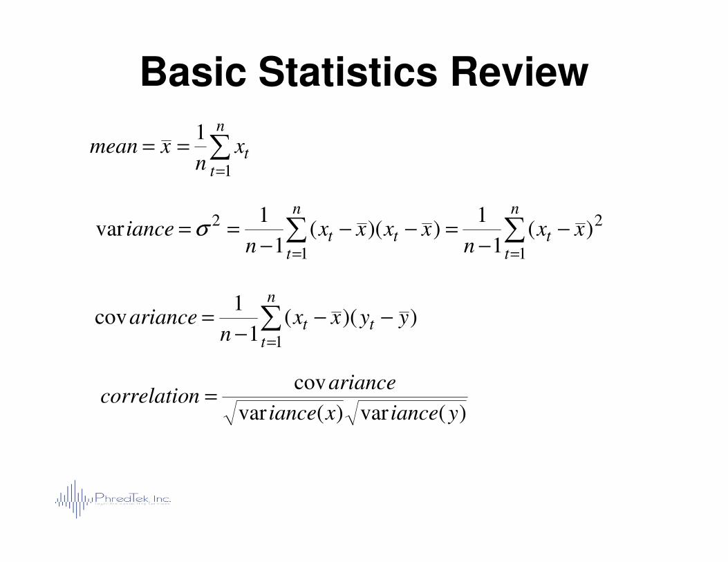
Basic Statistics Review
2
11
2 )(1
1))((
1
1var xx
nxxxx
niance
n
ttt
n
tt −
−=−−
−== ∑∑
==
σ
∑=
==
n
ttx
nxmean
1
1
))((1
1cov
1
yyxxn
ariance t
n
tt −−
−= ∑
=
)(var)(var
cov
yiancexiance
ariancencorrelatio =
Autocorrelation and Partial AutocorrelationAutocorrelation
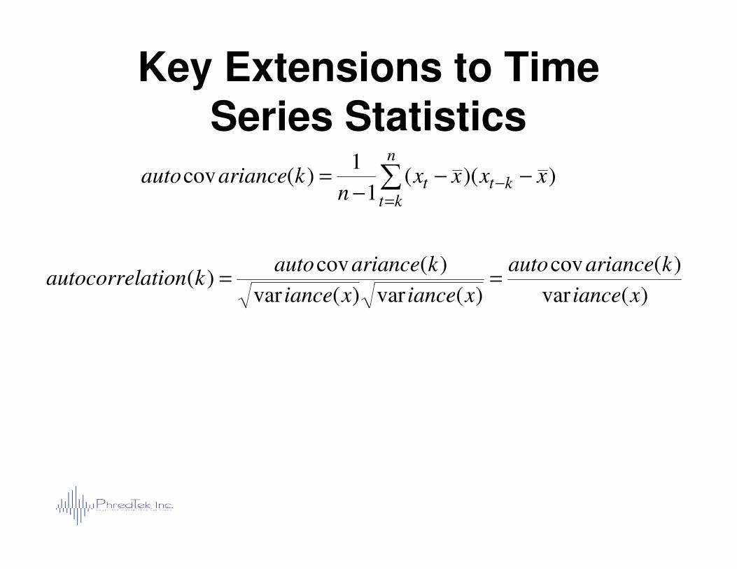
Key Extensions to Time Series Statistics
))((1
1)(cov xxxx
nkarianceauto kt
n
ktt −−
−= −
=
∑
)(var
)(cov
)(var)(var
)(cov)(
xiance
karianceauto
xiancexiance
karianceautokationautocorrel ==
)(var)(var)(var)(
xiancexiancexiancekationautocorrel ==
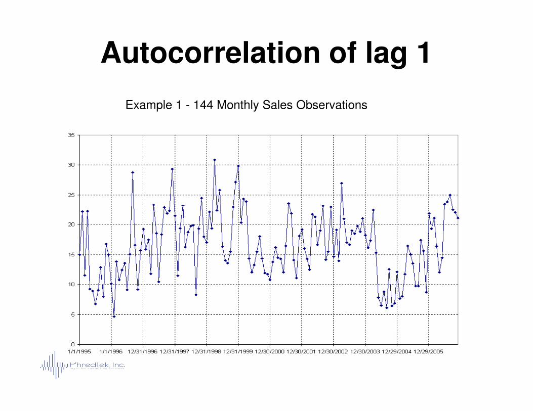
Autocorrelation of lag 1
Example 1 - 144 Monthly Sales Observations
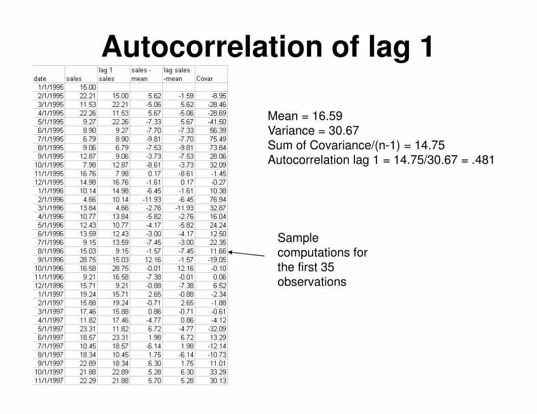
Autocorrelation of lag 1
Mean = 16.59Variance = 30.67Sum of Covariance/(n-1) = 14.75Autocorrelation lag 1 = 14.75/30.67 = .481
Sample computations for the first 35 observations
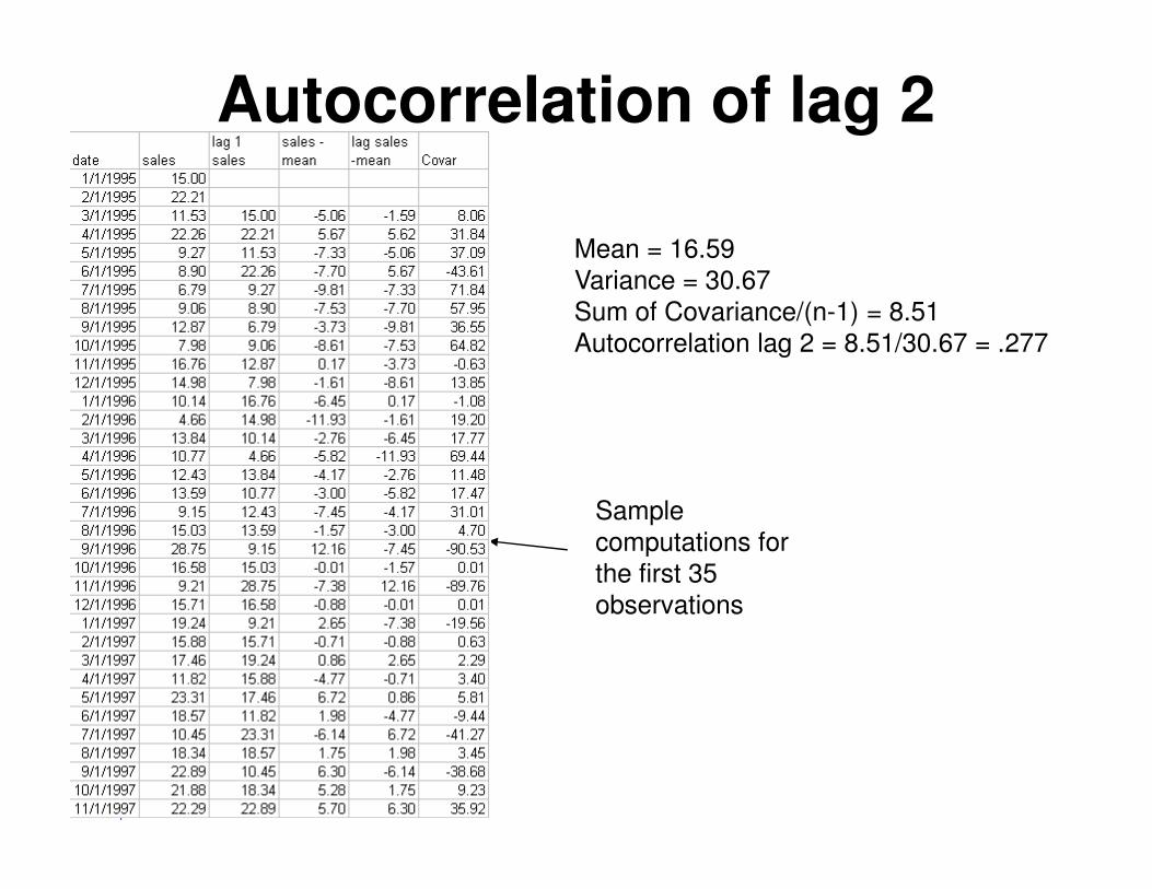
Autocorrelation of lag 2
Mean = 16.59Variance = 30.67Sum of Covariance/(n-1) = 8.51Autocorrelation lag 2 = 8.51/30.67 = .277
Sample computations for the first 35 observations
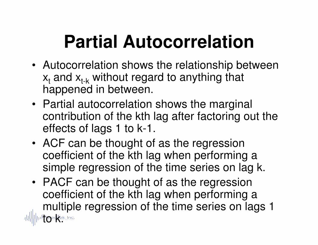
Partial Autocorrelation• Autocorrelation shows the relationship between
xt and xt-k without regard to anything that happened in between.
• Partial autocorrelation shows the marginal contribution of the kth lag after factoring out the effects of lags 1 to k-1.effects of lags 1 to k-1.
• ACF can be thought of as the regression coefficient of the kth lag when performing a simple regression of the time series on lag k.
• PACF can be thought of as the regression coefficient of the kth lag when performing a multiple regression of the time series on lags 1 to k.
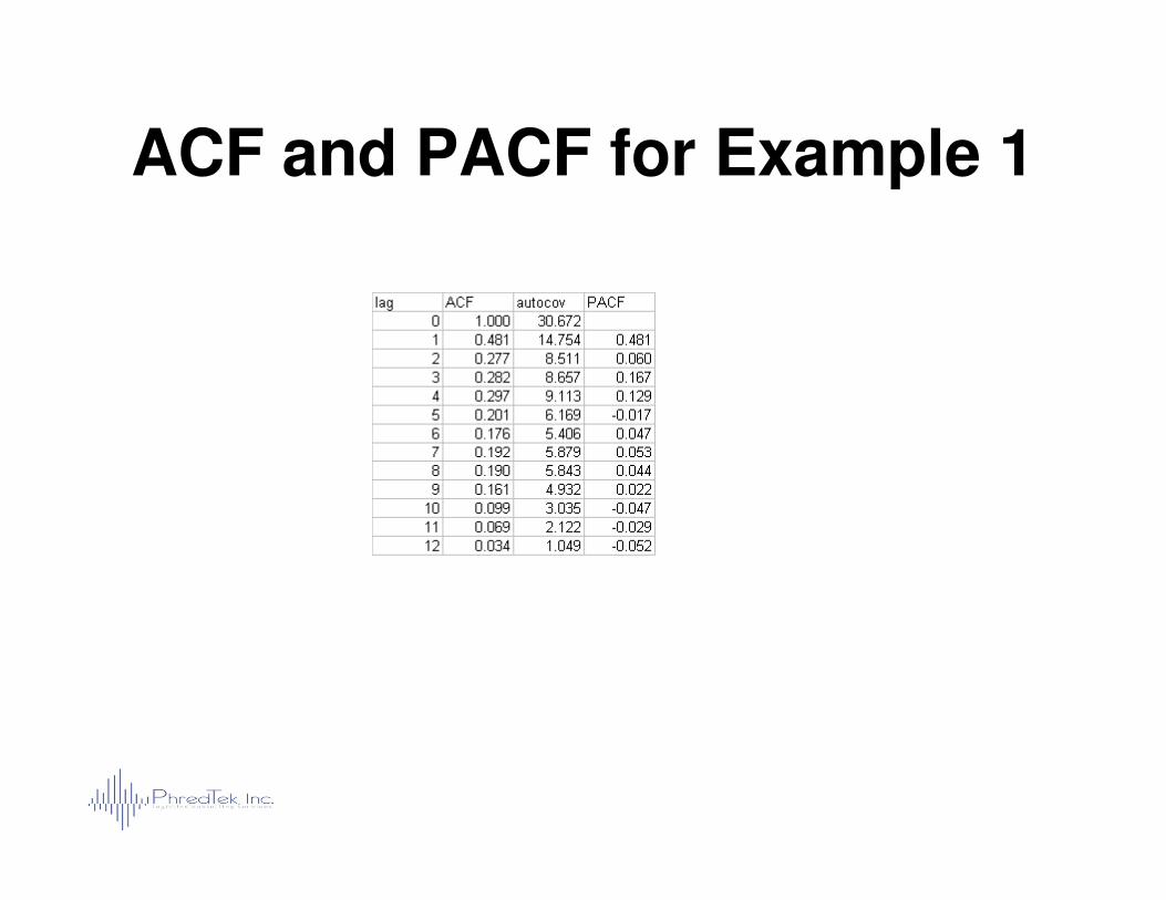
ACF and PACF for Example 1

The Family of ARIMA ModelsThe Family of ARIMA Models
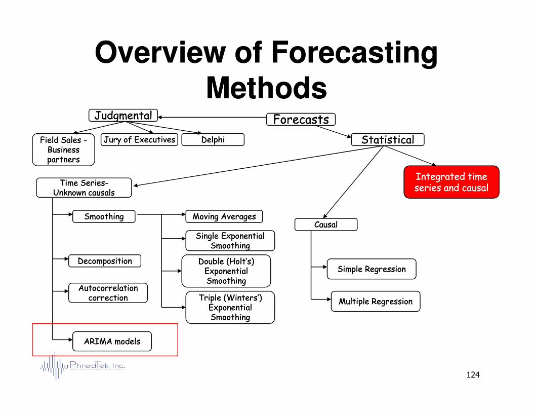
Overview of Forecasting Overview of Forecasting MethodsMethods
ForecastsForecastsJudgmentalJudgmental
StatisticalStatistical
Time SeriesTime Series--Unknown causalsUnknown causals
Integrated time Integrated time series and causalseries and causal
DelphiDelphiJury of ExecutivesJury of ExecutivesField Sales Field Sales --Business Business partnerspartners
124
CausalCausal
Autocorrelation Autocorrelation correctioncorrection
DecompositionDecomposition
SmoothingSmoothing Moving AveragesMoving Averages
Single Exponential Single Exponential SmoothingSmoothing
Double (Holt’s) Double (Holt’s) Exponential Exponential SmoothingSmoothing
Triple (Winters’) Triple (Winters’) Exponential Exponential SmoothingSmoothing
Simple RegressionSimple Regression
Multiple RegressionMultiple Regression
ARIMA modelsARIMA models
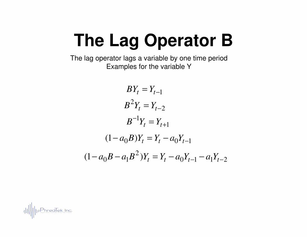
The Lag Operator BThe lag operator lags a variable by one time period
Examples for the variable Y
1−= tt YBY
22
−= tt YYB
1−= YYB 1
1+
−= tt YYB
100 )1( −−=− ttt YaYYBa
21102
10 )1( −− −−=−− tttt YaYaYYBaBa
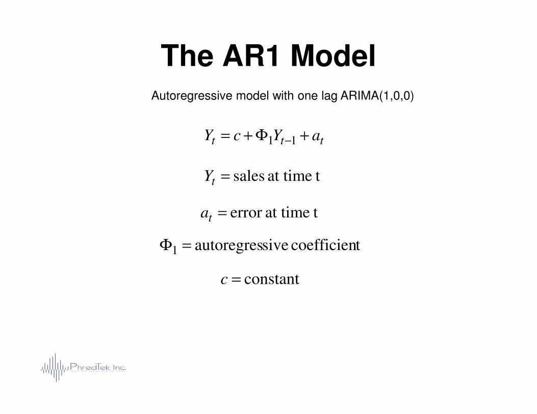
The AR1 ModelAutoregressive model with one lag ARIMA(1,0,0)
ttt aYcY +Φ+= −11
tat time sales=tY
tat timeerror =a tat timeerror =ta
tcoefficien siveautoregres1 =Φ
constant=c
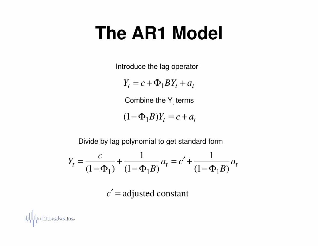
The AR1 Model
Introduce the lag operator
Combine the Yt terms
tt acYB +=Φ− )1( 1
ttt aBYcY +Φ+= 1
constant adjusted=′c
Divide by lag polynomial to get standard form
ttt aB
caB
cY
)1(
1
)1(
1
)1( 111 Φ−+′=
Φ−+
Φ−=
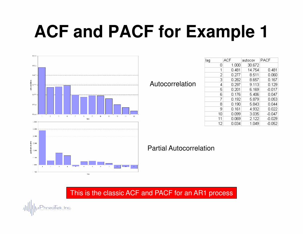
ACF and PACF for Example 1
Autocorrelation
Partial Autocorrelation
This is the classic ACF and PACF for an AR1 process
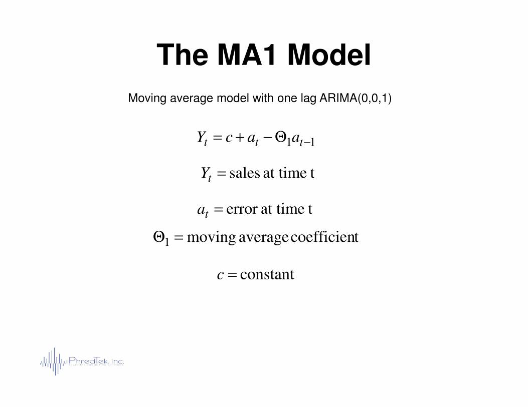
The MA1 Model
Moving average model with one lag ARIMA(0,0,1)
tat time sales=tY
tat timeerror =a
11 −Θ−+= ttt aacY
tat timeerror =ta
constant=c
tcoefficien average moving1 =Θ
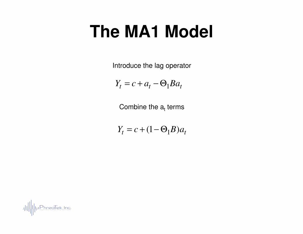
The MA1 Model
Introduce the lag operator
Combine the at terms
ttt BaacY 1Θ−+=
tt aBcY )1( 1Θ−+=
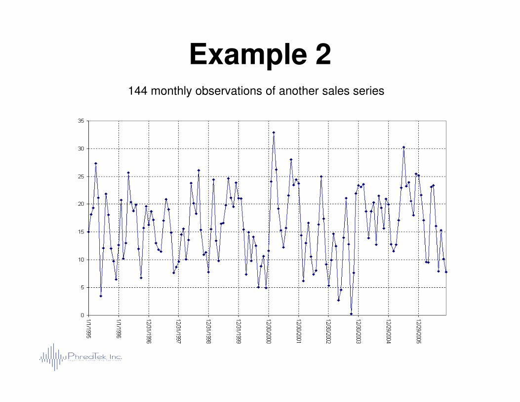
Example 2144 monthly observations of another sales series
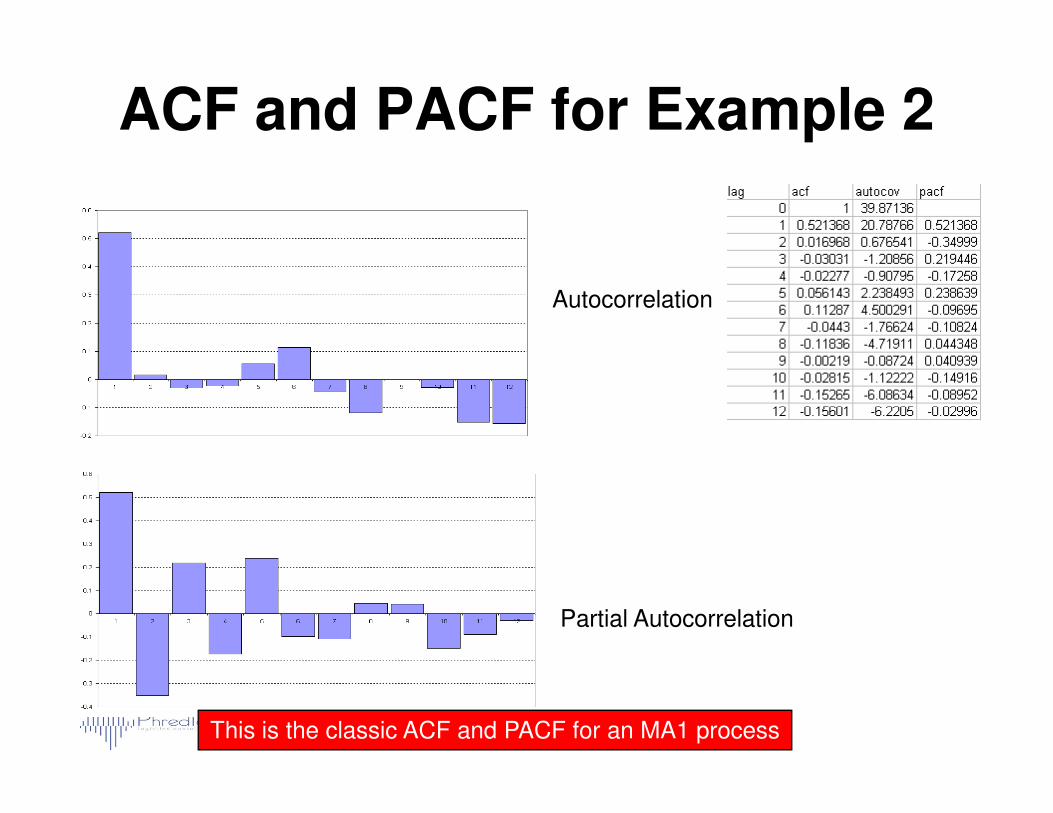
ACF and PACF for Example 2
Autocorrelation
Partial Autocorrelation
This is the classic ACF and PACF for an MA1 process
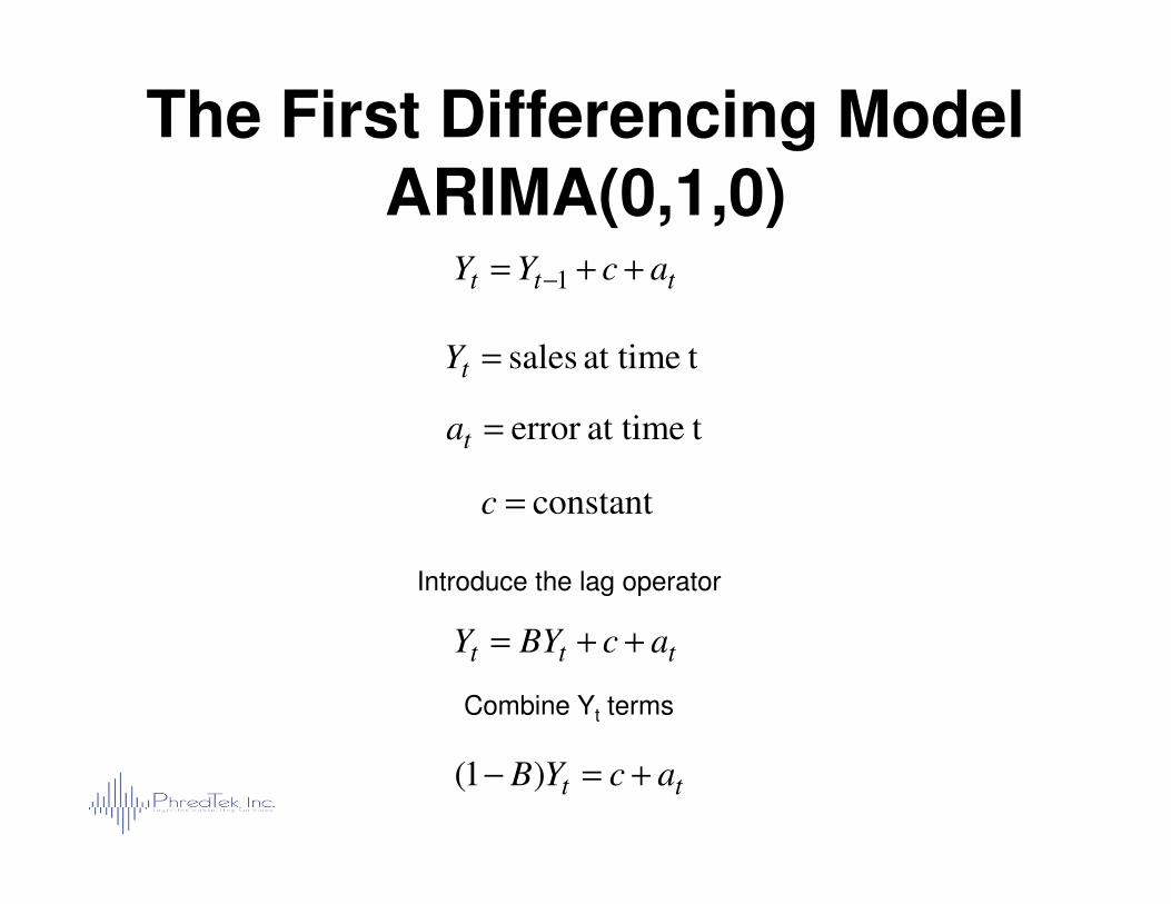
The First Differencing ModelARIMA(0,1,0)
tat time sales=tY
tat timeerror =ta
ttt acYY ++= −1
constant=c
Introduce the lag operator
ttt acBYY ++=
Combine Yt terms
tt acYB +=− )1(
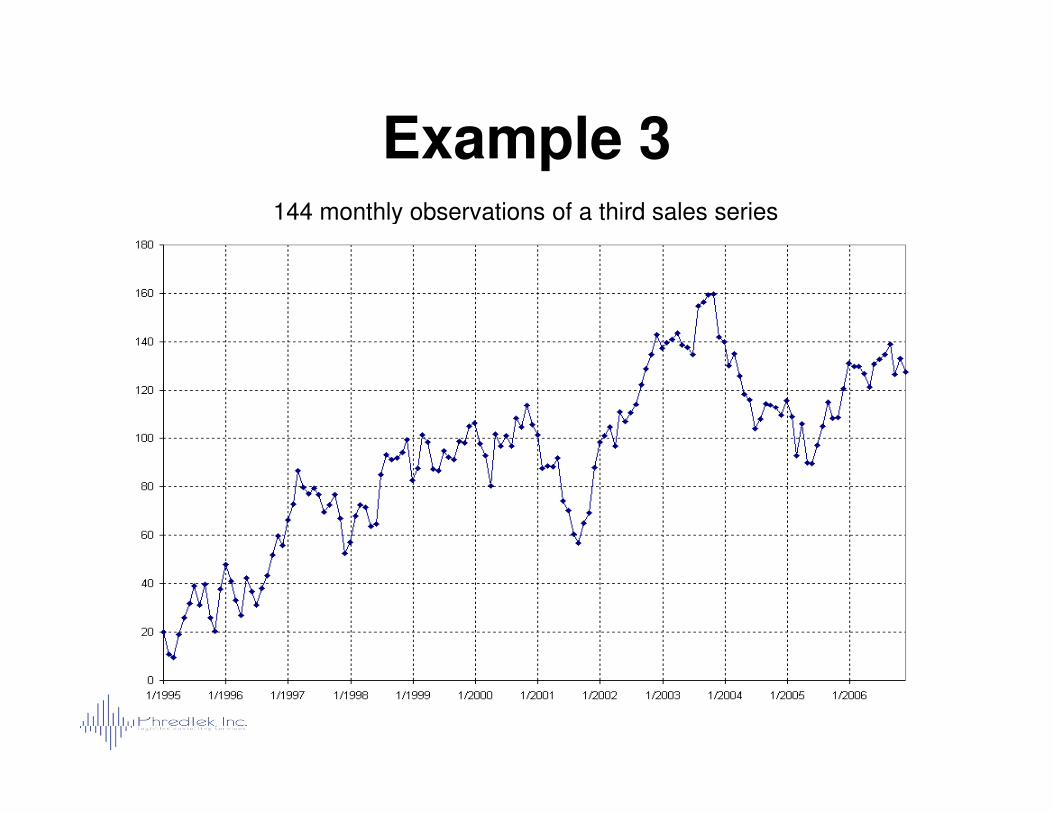
Example 3144 monthly observations of a third sales series
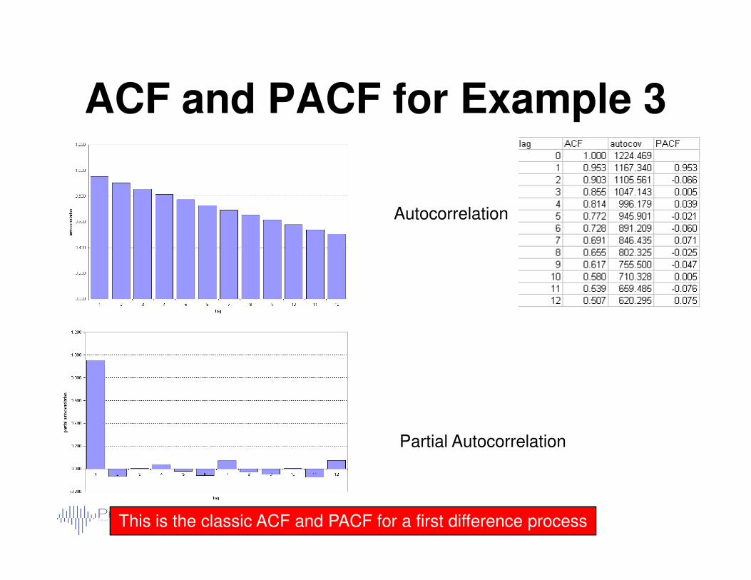
ACF and PACF for Example 3
Autocorrelation
Partial Autocorrelation
This is the classic ACF and PACF for a first difference process
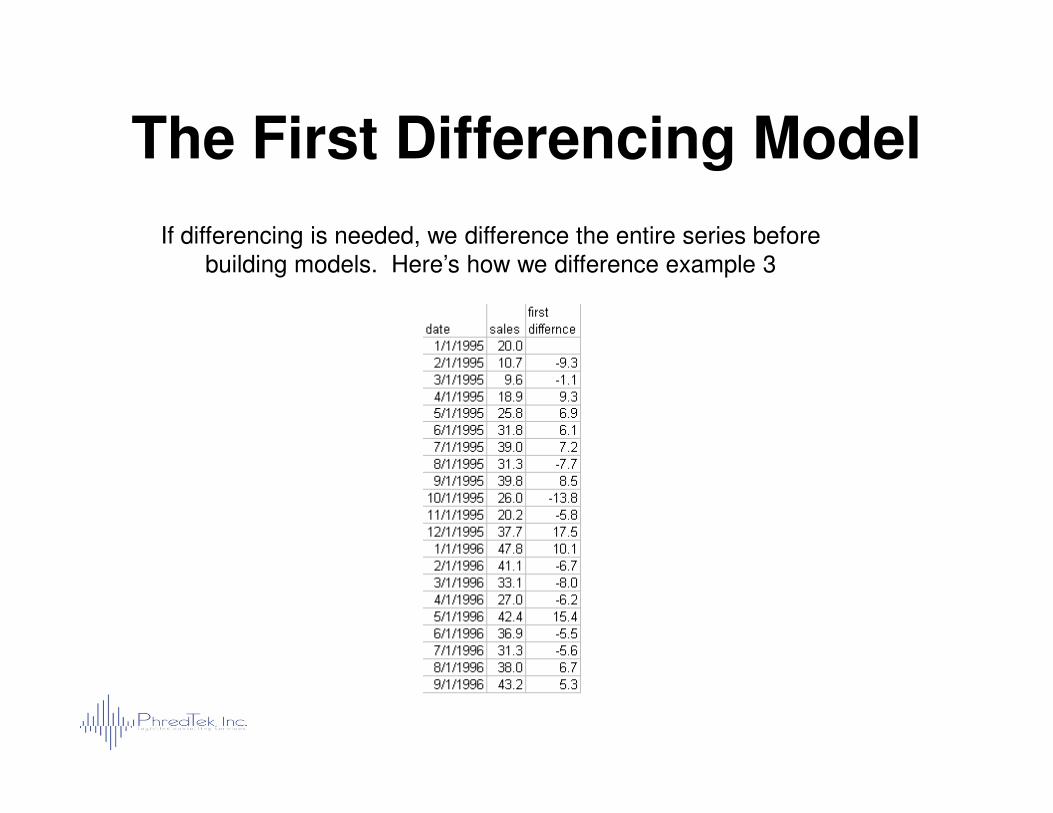
The First Differencing Model
If differencing is needed, we difference the entire series before building models. Here’s how we difference example 3
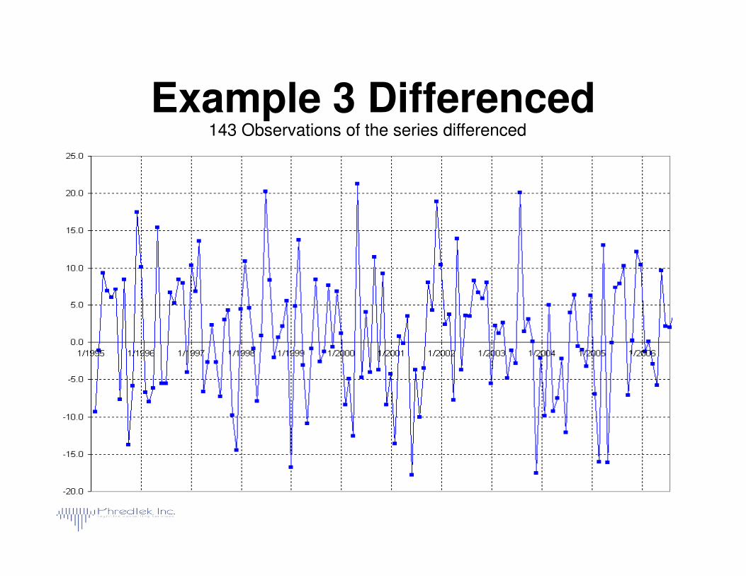
Example 3 Differenced143 Observations of the series differenced
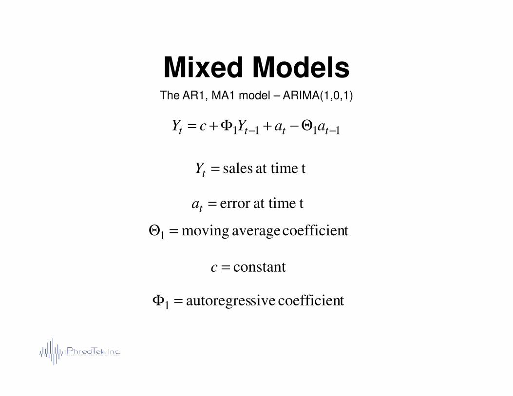
Mixed ModelsThe AR1, MA1 model – ARIMA(1,0,1)
tat time sales=tY
tat timeerror =a
1111 −− Θ−+Φ+= tttt aaYcY
tat timeerror =ta
constant=c
tcoefficien average moving1 =Θ
tcoefficien siveautoregres1 =Φ
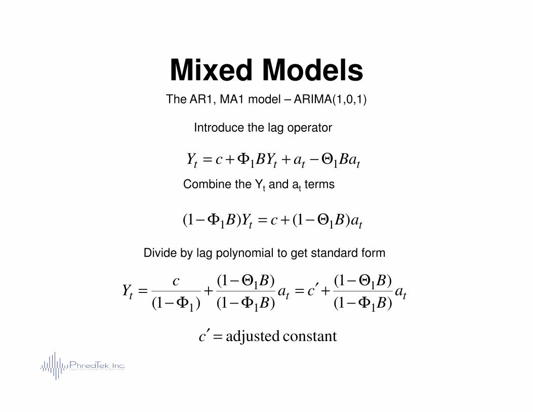
Mixed Models
Introduce the lag operator
tttt BaaBYcY 11 Θ−+Φ+=
Combine the Yt and at terms
The AR1, MA1 model – ARIMA(1,0,1)
tt aBcYB )1()1( 11 Θ−+=Φ−
Divide by lag polynomial to get standard form
ttt aB
Bca
B
BcY
)1(
)1(
)1(
)1(
)1( 1
1
1
1
1 Φ−
Θ−+′=
Φ−
Θ−+
Φ−=
constant adjusted=′c
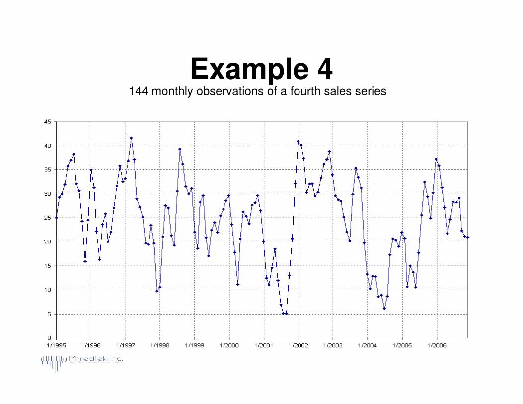
Example 4144 monthly observations of a fourth sales series
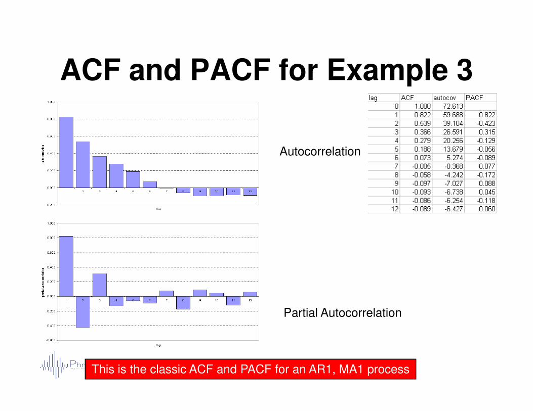
ACF and PACF for Example 3
Autocorrelation
Partial Autocorrelation
This is the classic ACF and PACF for an AR1, MA1 process
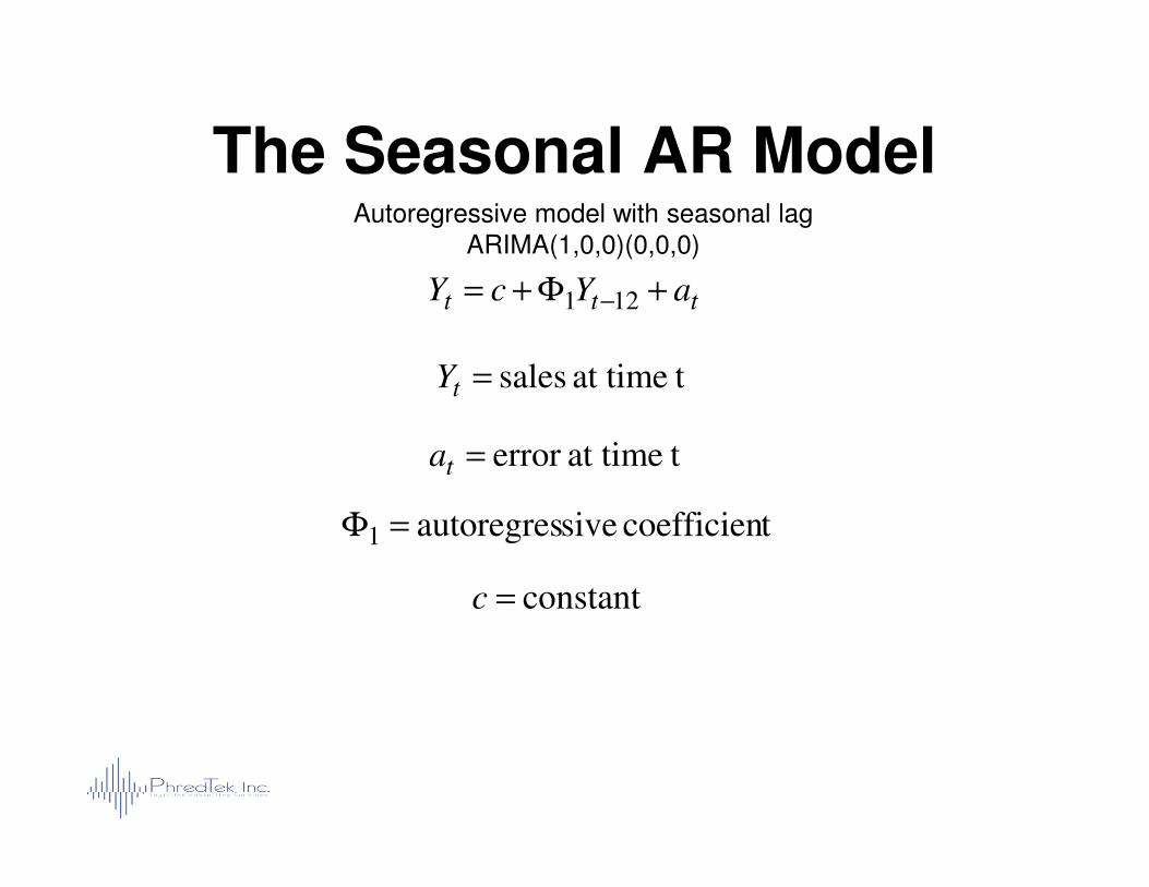
The Seasonal AR ModelAutoregressive model with seasonal lag
ARIMA(1,0,0)(0,0,0)
tat time sales=tY
tat timeerror =a
ttt aYcY +Φ+= −121
tat timeerror =ta
tcoefficien siveautoregres1 =Φ
constant=c
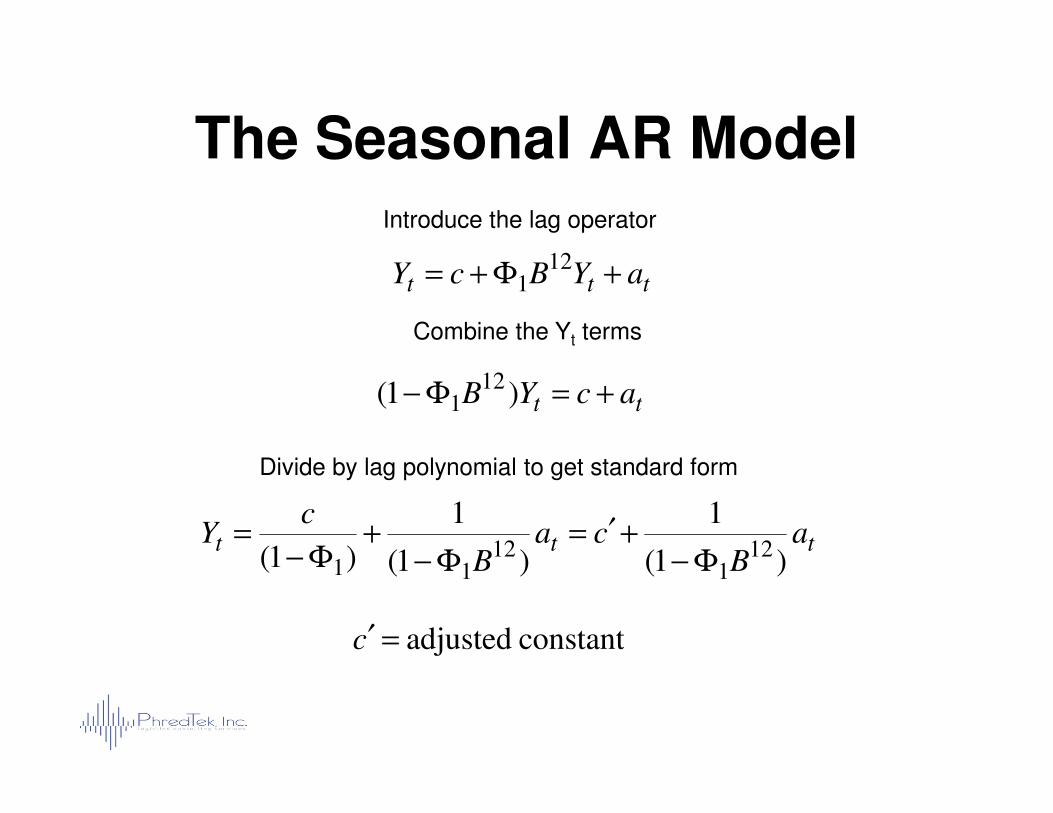
The Seasonal AR ModelIntroduce the lag operator
Combine the Yt terms
ttt aYBcY +Φ+=12
1
tt acYB +=Φ− )1( 121
constant adjusted=′c
Divide by lag polynomial to get standard form
tt acYB +=Φ− )1( 1
ttt aB
caB
cY
)1(
1
)1(
1
)1( 121
1211 Φ−
+′=Φ−
+Φ−
=
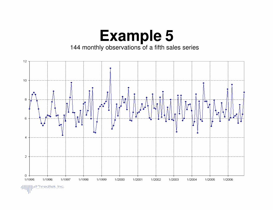
Example 5144 monthly observations of a fifth sales series
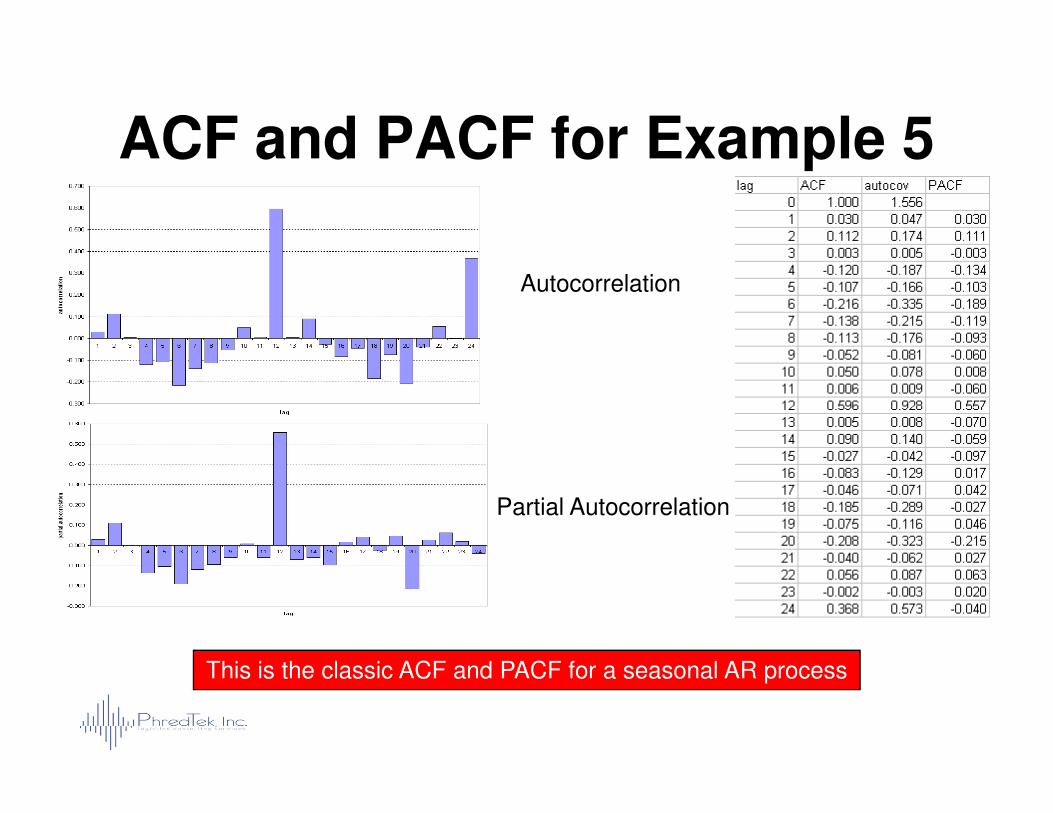
ACF and PACF for Example 5
Autocorrelation
Partial Autocorrelation
This is the classic ACF and PACF for a seasonal AR process
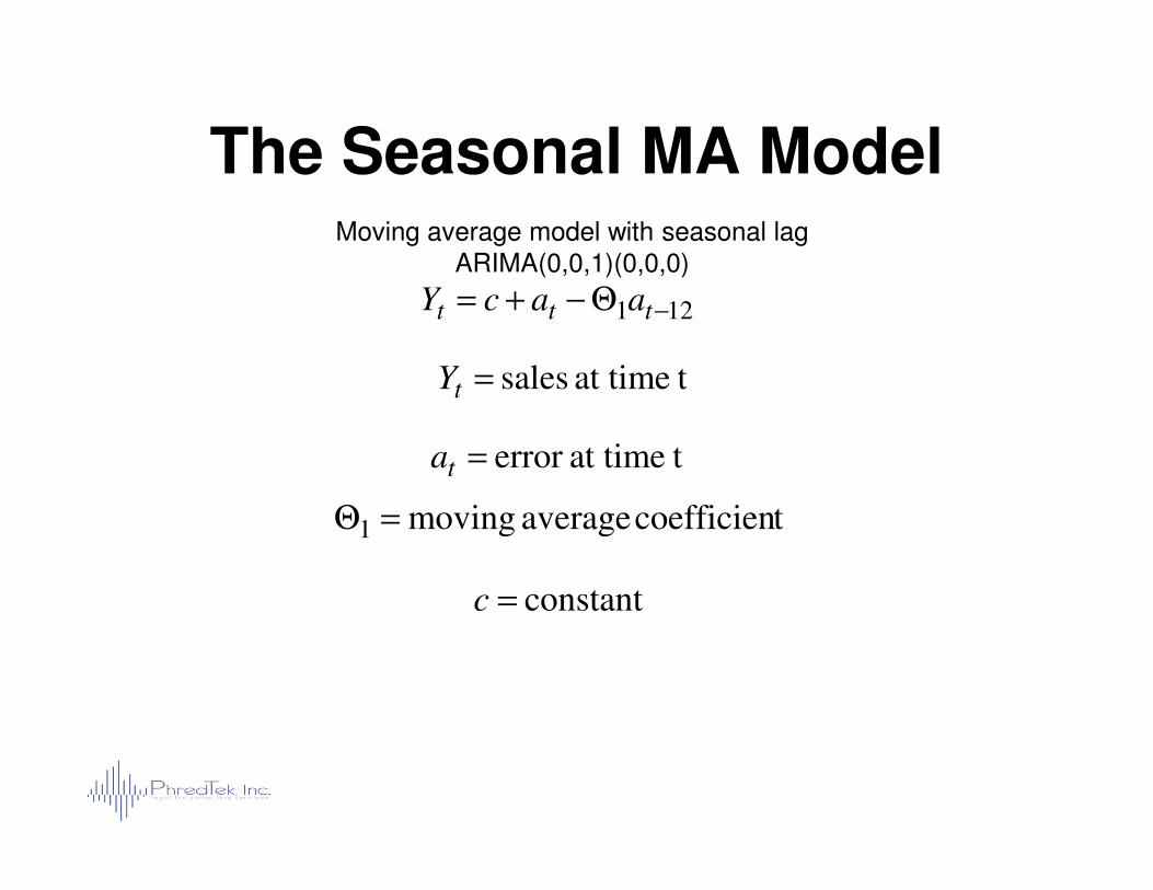
The Seasonal MA ModelMoving average model with seasonal lag
ARIMA(0,0,1)(0,0,0)
tat time sales=tY
tat timeerror =a
121 −Θ−+= ttt aacY
tat timeerror =ta
constant=c
tcoefficien average moving1 =Θ
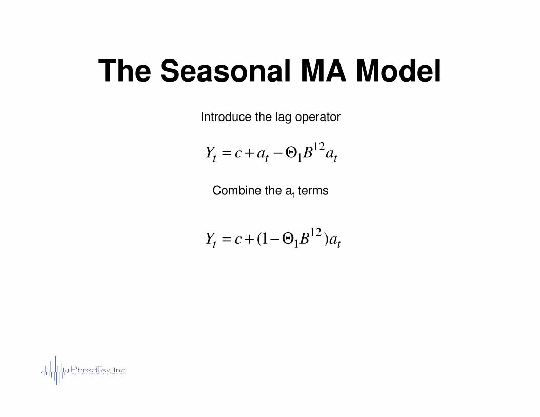
Introduce the lag operator
Combine the at terms
The Seasonal MA Model
ttt aBacY12
1Θ−+=
tt aBcY )1( 121Θ−+=
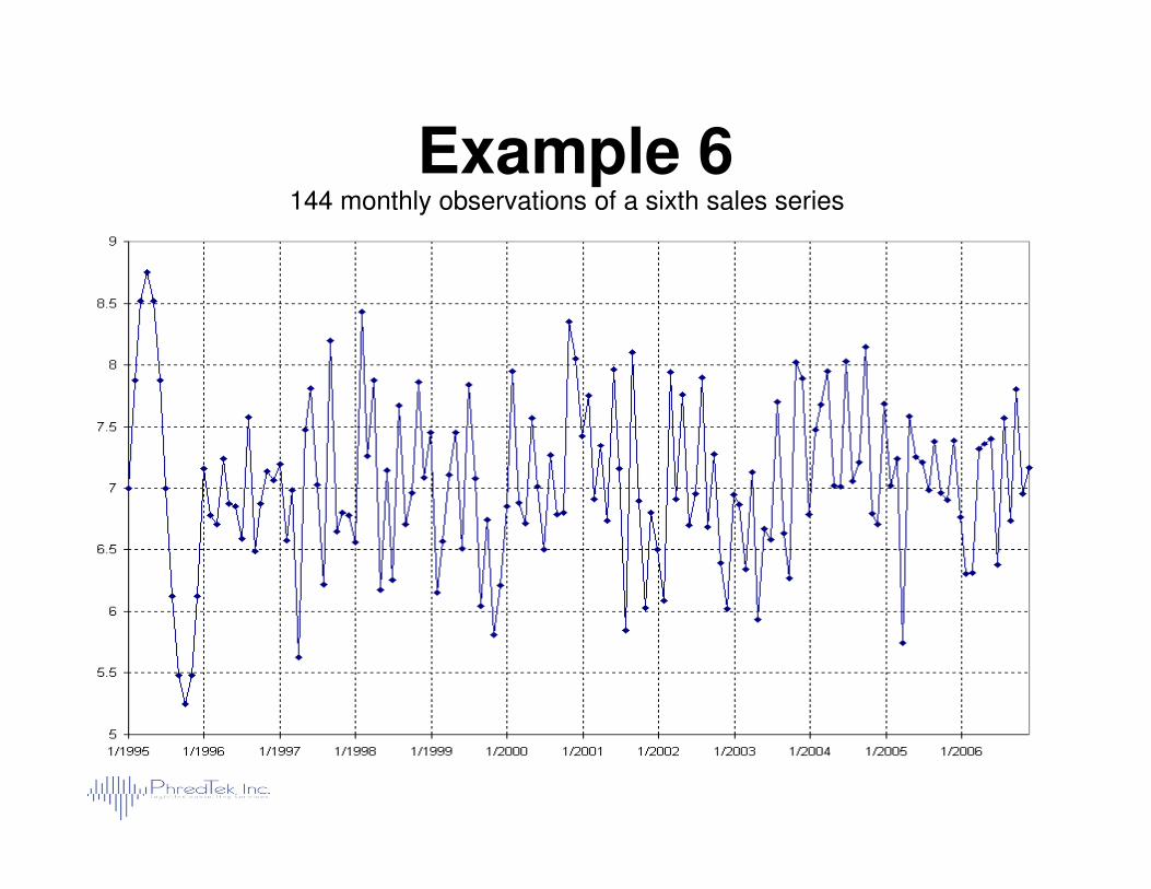
Example 6144 monthly observations of a sixth sales series
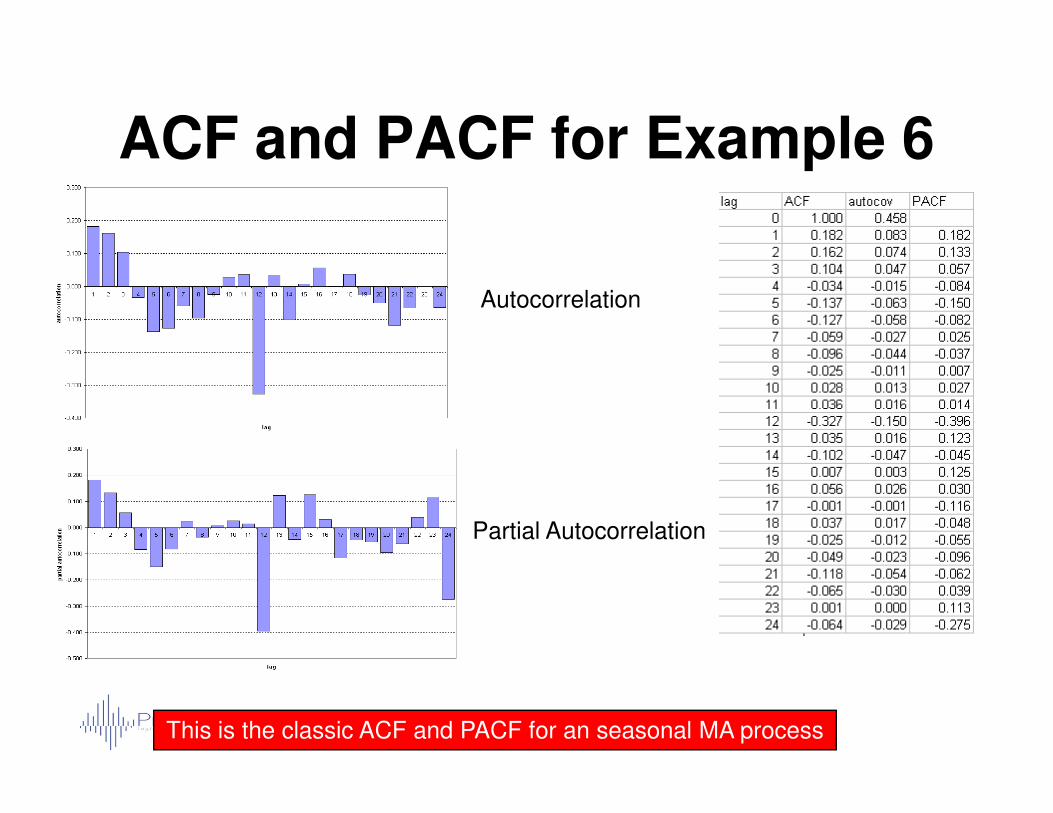
ACF and PACF for Example 6
Autocorrelation
Partial Autocorrelation
This is the classic ACF and PACF for an seasonal MA process
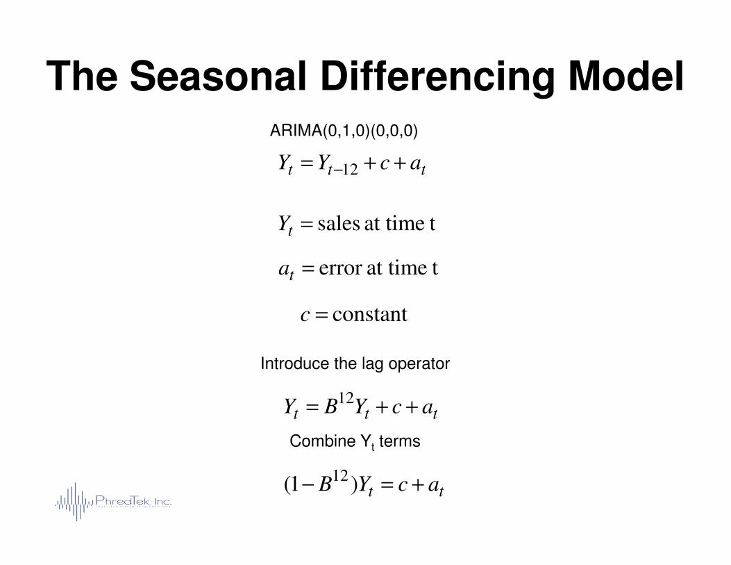
The Seasonal Differencing Model
tat time sales=tY
tat timeerror =ta
ttt acYY ++= −12
ARIMA(0,1,0)(0,0,0)
constant=c
Introduce the lag operator
Combine Yt terms
ttt acYBY ++=12
tt acYB +=− )1( 12
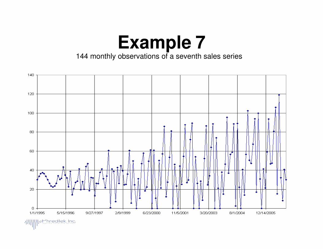
Example 7144 monthly observations of a seventh sales series
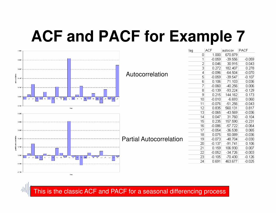
ACF and PACF for Example 7
Autocorrelation
Partial Autocorrelation
This is the classic ACF and PACF for a seasonal differencing process
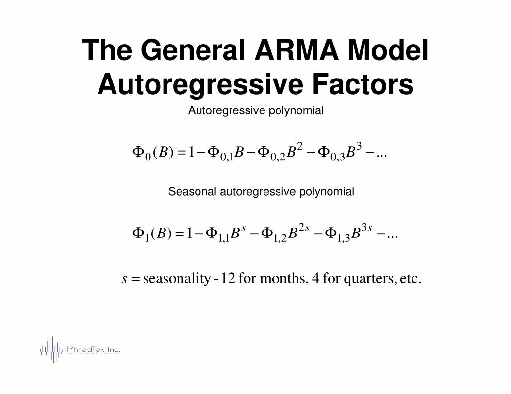
Autoregressive polynomial
The General ARMA ModelAutoregressive Factors
...1)( 33,0
22,01,00 −Φ−Φ−Φ−=Φ BBBB
Seasonal autoregressive polynomialSeasonal autoregressive polynomial
etc. quarters,for 4 months,for 12 -yseasonalit=s
...1)( 33,1
22,11,11 −Φ−Φ−Φ−=Φ
sssBBBB
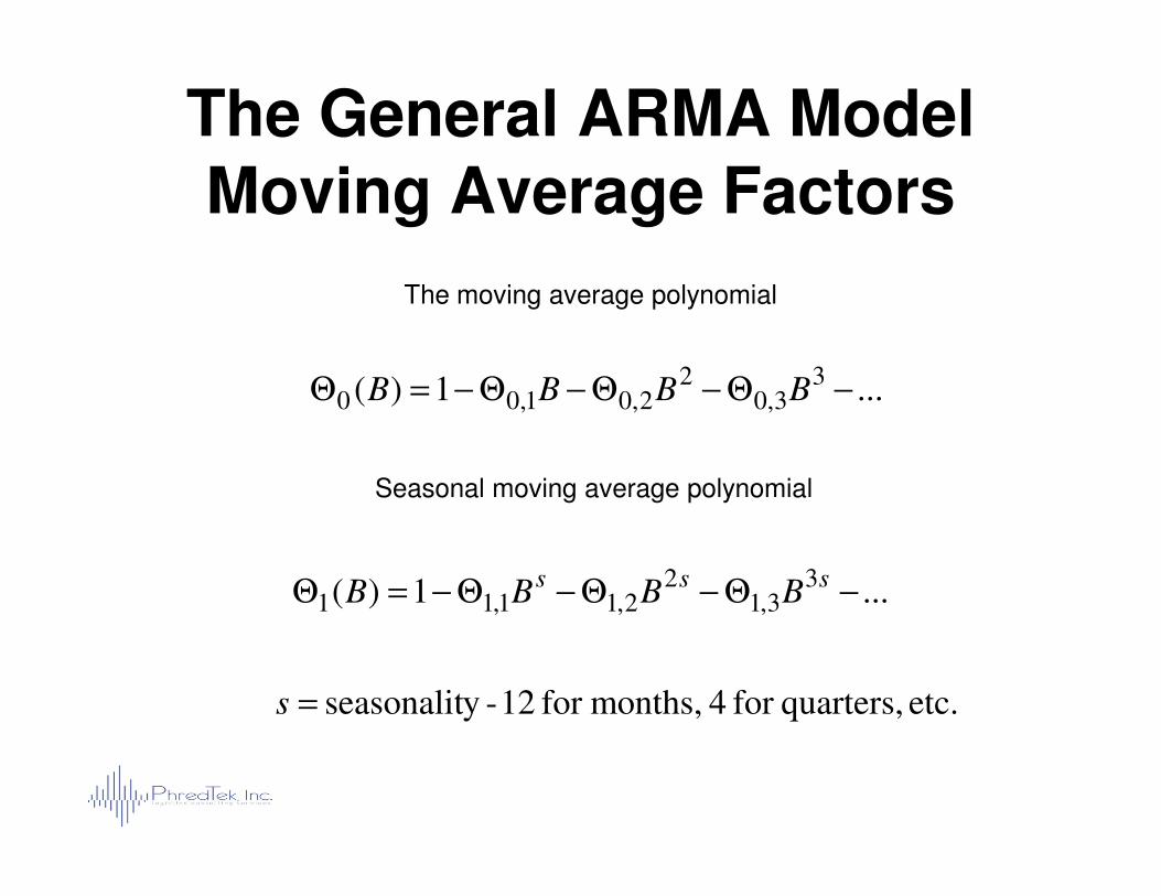
The moving average polynomial
The General ARMA ModelMoving Average Factors
...1)( 33,0
22,01,00 −Θ−Θ−Θ−=Θ BBBB
etc. quarters,for 4 months,for 12 -yseasonalit=s
Seasonal moving average polynomial
...1)( 33,1
22,11,11 −Θ−Θ−Θ−=Θ
sssBBBB
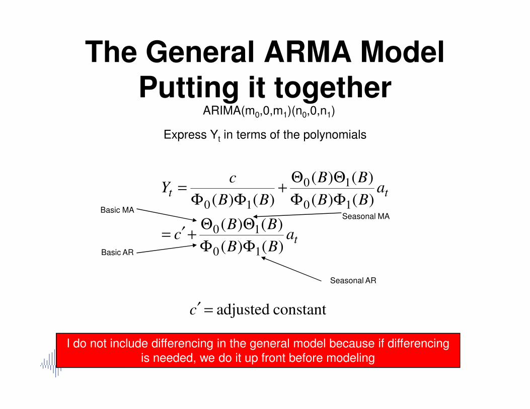
Express Yt in terms of the polynomials
The General ARMA ModelPutting it together
tt aBB
BB
BB
cY
)()(
)()(
)()( 10
10
10 ΦΦ
ΘΘ+
ΦΦ=
ARIMA(m0,0,m1)(n0,0,n1)
taBB
BBc
BBBB
)()(
)()(
)()()()(
10
10
1010
ΦΦ
ΘΘ+′=
ΦΦΦΦ
constant adjusted=′c
I do not include differencing in the general model because if differencing is needed, we do it up front before modeling
Basic MA
Basic AR
Seasonal MA
Seasonal AR
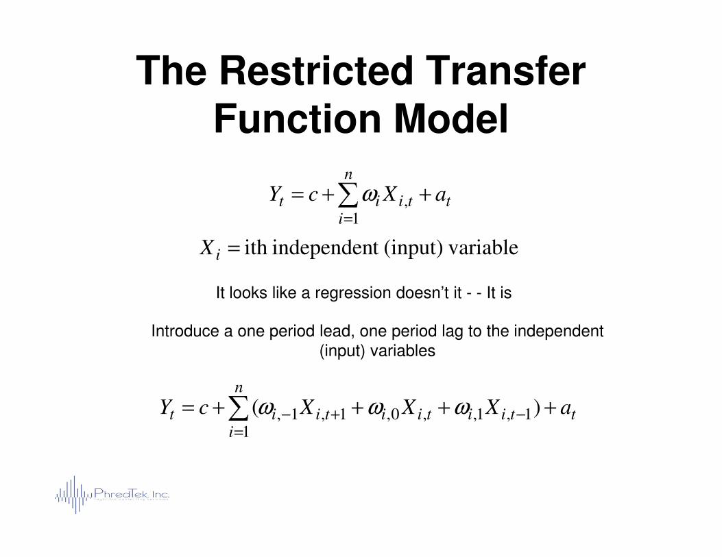
The Restricted Transfer Function Model
t
n
itiit aXcY ++= ∑
=1,ω
variable(input)t independenith =iX
It looks like a regression doesn’t it - - It is
Introduce a one period lead, one period lag to the independent (input) variables
ttiitiitii
n
it aXXXcY ++++= −+−
=
∑ )( 1,1,,0,1,1,1
ωωω
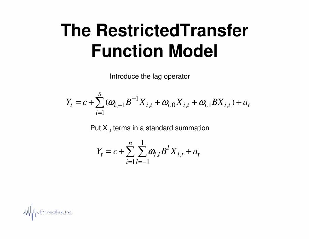
The RestrictedTransfer Function Model
Introduce the lag operator
ttiitiitii
n
it aBXXXBcY ++++=
−−
=
∑ )( ,1,,0,,1
1,1
ωωω
Put Xi,t terms in a standard summation
t
n
i lti
llit aXBcY ++= ∑ ∑
= −=1
1
1,,ω

Overview of Forecasting Overview of Forecasting MethodsMethods
ForecastsForecastsJudgmentalJudgmental
StatisticalStatistical
Time SeriesTime Series--Unknown causalsUnknown causals
Integrated time Integrated time series and causalseries and causal
DelphiDelphiJury of ExecutivesJury of ExecutivesField Sales Field Sales --Business Business partnerspartners
158
CausalCausal
Autocorrelation Autocorrelation correctioncorrection
DecompositionDecomposition
SmoothingSmoothing Moving AveragesMoving Averages
Single Exponential Single Exponential SmoothingSmoothing
Double (Holt’s) Double (Holt’s) Exponential Exponential SmoothingSmoothing
Triple (Winters’) Triple (Winters’) Exponential Exponential SmoothingSmoothing
Simple RegressionSimple Regression
Multiple RegressionMultiple Regression
ARIMA modelsARIMA models
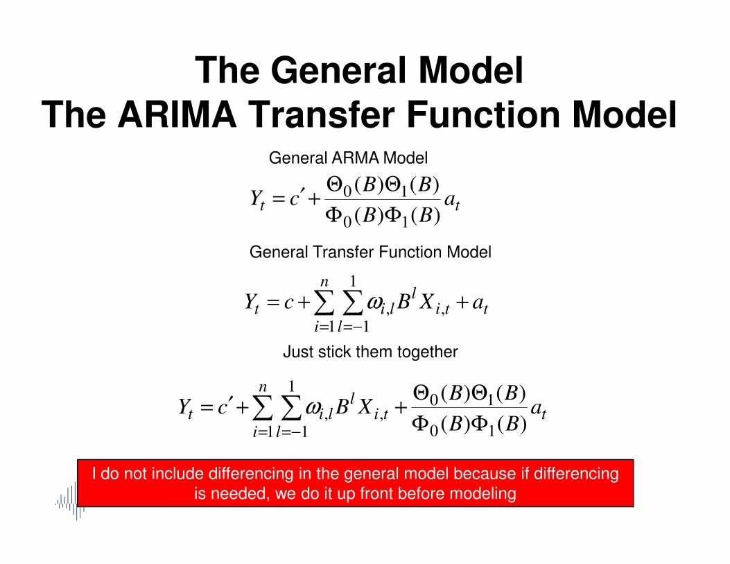
The General ModelThe ARIMA Transfer Function Model
General ARMA Model
General Transfer Function Model
n 1
tt aBB
BBcY
)()(
)()(
10
10
ΦΦ
ΘΘ+′=
t
n
i lti
llit aXBcY ++= ∑ ∑
= −=1
1
1,,ω
Just stick them together
t
n
i lti
llit a
BB
BBXBcY
)()(
)()(
10
10
1
1
1,,
ΦΦ
ΘΘ++′= ∑ ∑
= −=
ω
I do not include differencing in the general model because if differencing is needed, we do it up front before modeling
The Modeling ProcessThe Modeling Process
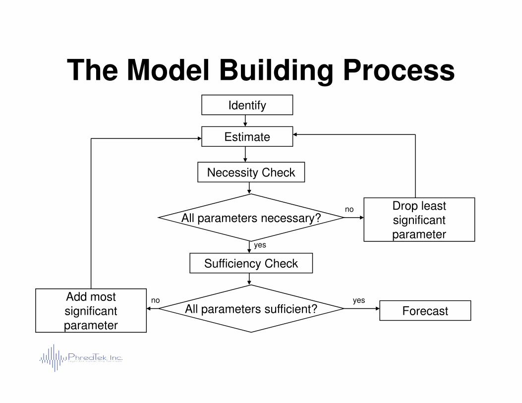
The Model Building ProcessIdentify
Estimate
Necessity Check
Drop least
Sufficiency Check
All parameters necessary?
All parameters sufficient? Forecast
Drop least significant parameter
Add most significant parameter
no
yes
no
yes
General Mills Biscuits ExampleExample
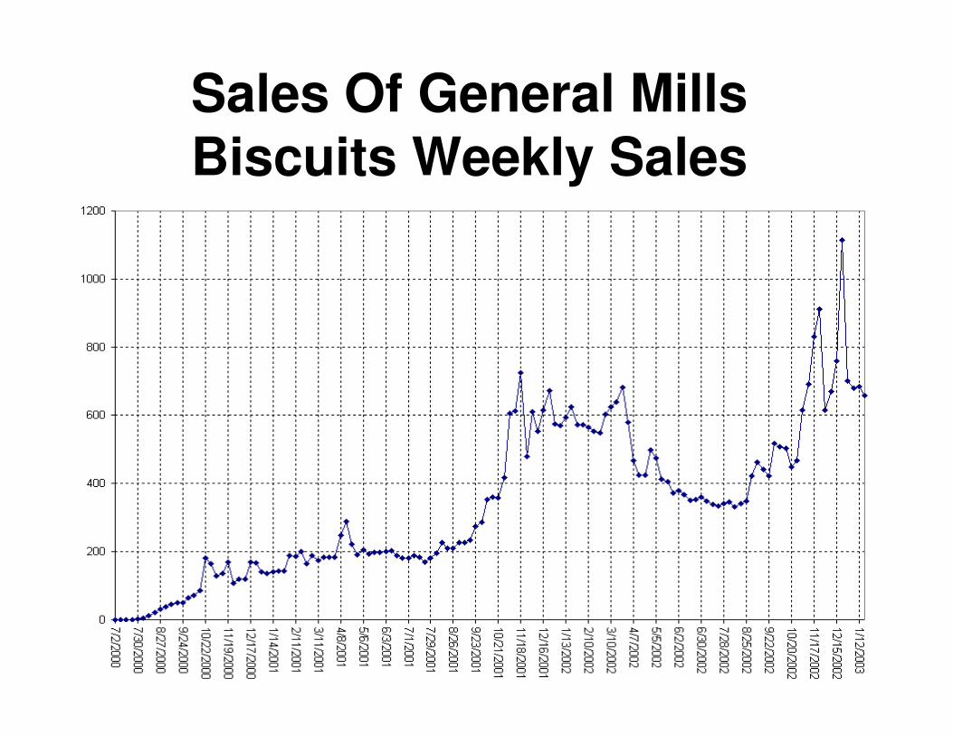
Sales Of General Mills Biscuits Weekly Sales
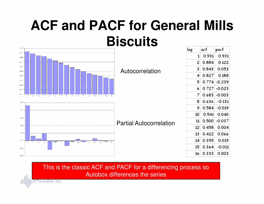
ACF and PACF for General Mills Biscuits
Autocorrelation
Partial Autocorrelation
This is the classic ACF and PACF for a differencing process so Autobox differences the series
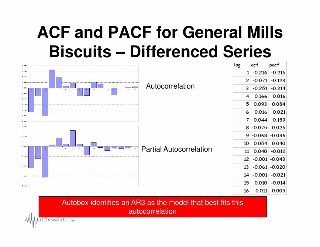
ACF and PACF for General Mills Biscuits – Differenced Series
Autocorrelation
Partial Autocorrelation
Autobox identifies an AR3 as the model that best fits this autocorrelation
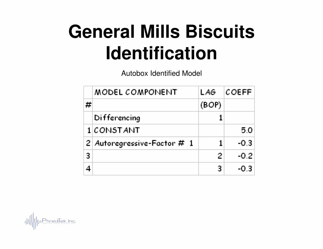
General Mills BiscuitsIdentification
Autobox Identified Model

The Model Building ProcessIdentify
Estimate
Necessity Check
Drop least
Sufficiency Check
All parameters necessary?
All parameters sufficient? Forecast
Drop least significant parameter
Add most significant parameter
no
yes
no
yes
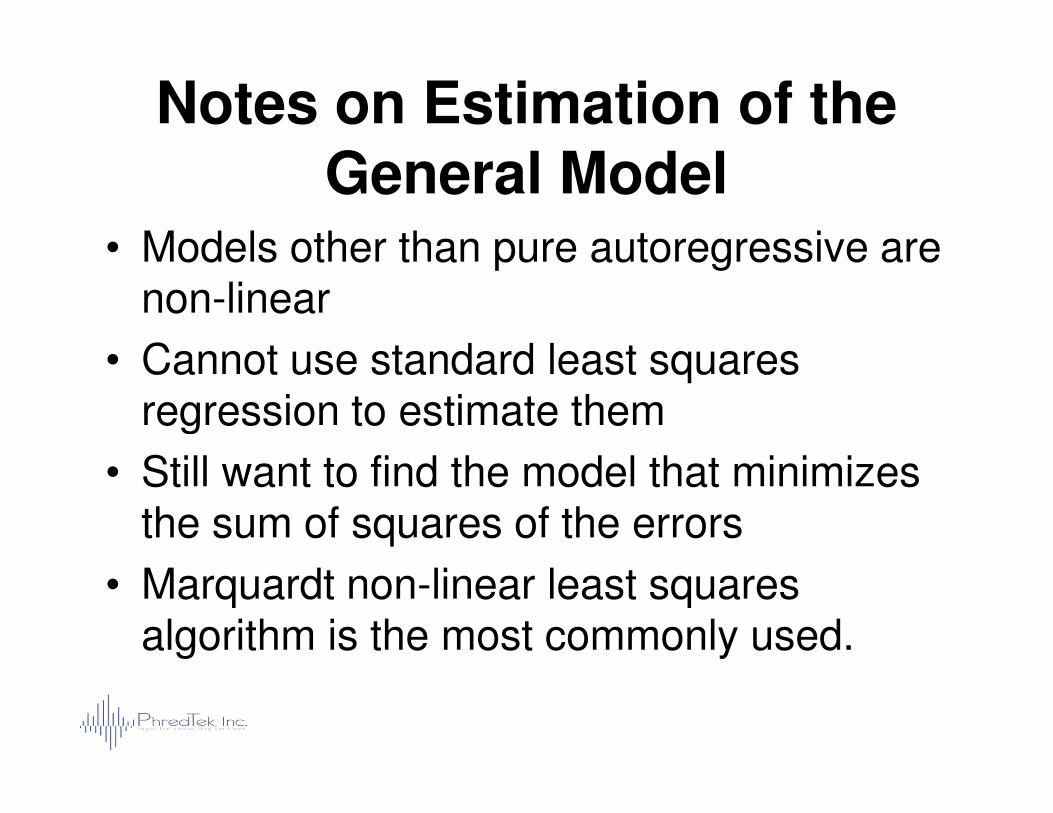
Notes on Estimation of the General Model
• Models other than pure autoregressive are non-linear
• Cannot use standard least squares regression to estimate themregression to estimate them
• Still want to find the model that minimizes the sum of squares of the errors
• Marquardt non-linear least squares algorithm is the most commonly used.
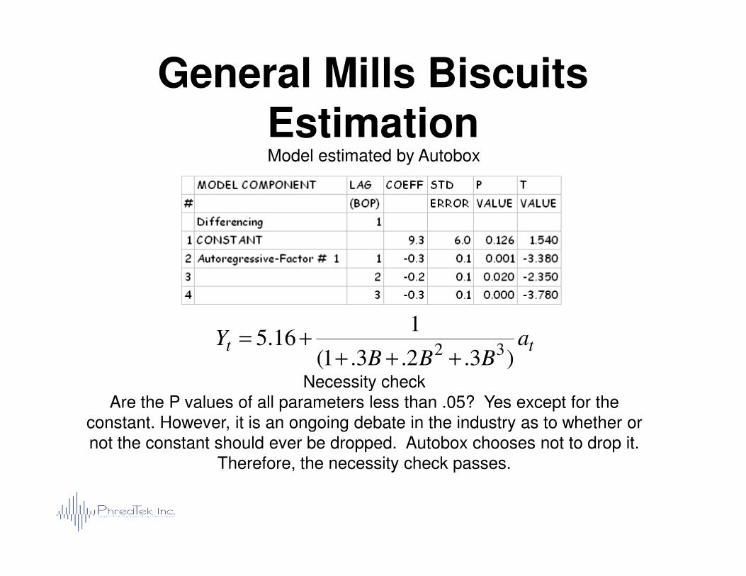
General Mills BiscuitsEstimationModel estimated by Autobox
Necessity checkAre the P values of all parameters less than .05? Yes except for the
constant. However, it is an ongoing debate in the industry as to whether or not the constant should ever be dropped. Autobox chooses not to drop it.
Therefore, the necessity check passes.
tt aBBB
Y)3.2.3.1(
116.5
32+++
+=

The Model Building ProcessIdentify
Estimate
Necessity Check
Drop least
Sufficiency Check
All parameters necessary?
All parameters sufficient? Forecast
Drop least significant parameter
Add most significant parameter
no
yes
no
yes
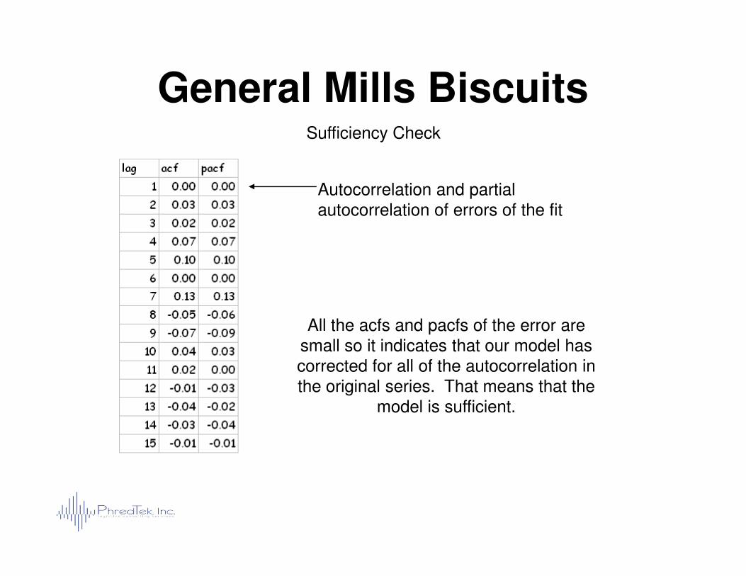
Autocorrelation and partial autocorrelation of errors of the fit
General Mills BiscuitsSufficiency Check
All the acfs and pacfs of the error are small so it indicates that our model has corrected for all of the autocorrelation in the original series. That means that the
model is sufficient.
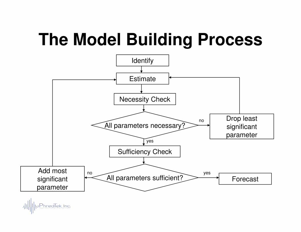
The Model Building ProcessIdentify
Estimate
Necessity Check
Drop least
Sufficiency Check
All parameters necessary?
All parameters sufficient? Forecast
Drop least significant parameter
Add most significant parameter
no
yes
no
yes
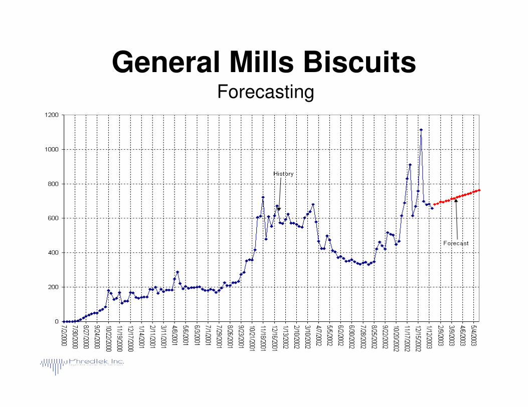
General Mills BiscuitsForecasting
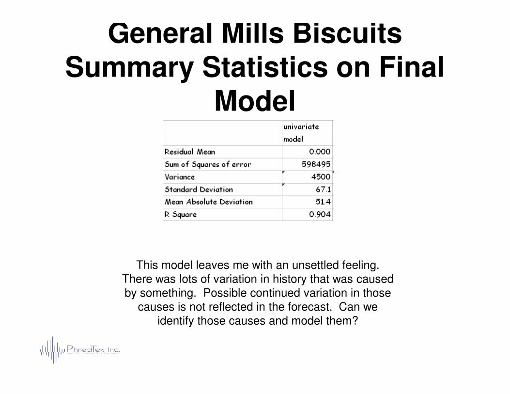
General Mills BiscuitsSummary Statistics on Final
Model
This model leaves me with an unsettled feeling. There was lots of variation in history that was caused by something. Possible continued variation in those
causes is not reflected in the forecast. Can we identify those causes and model them?
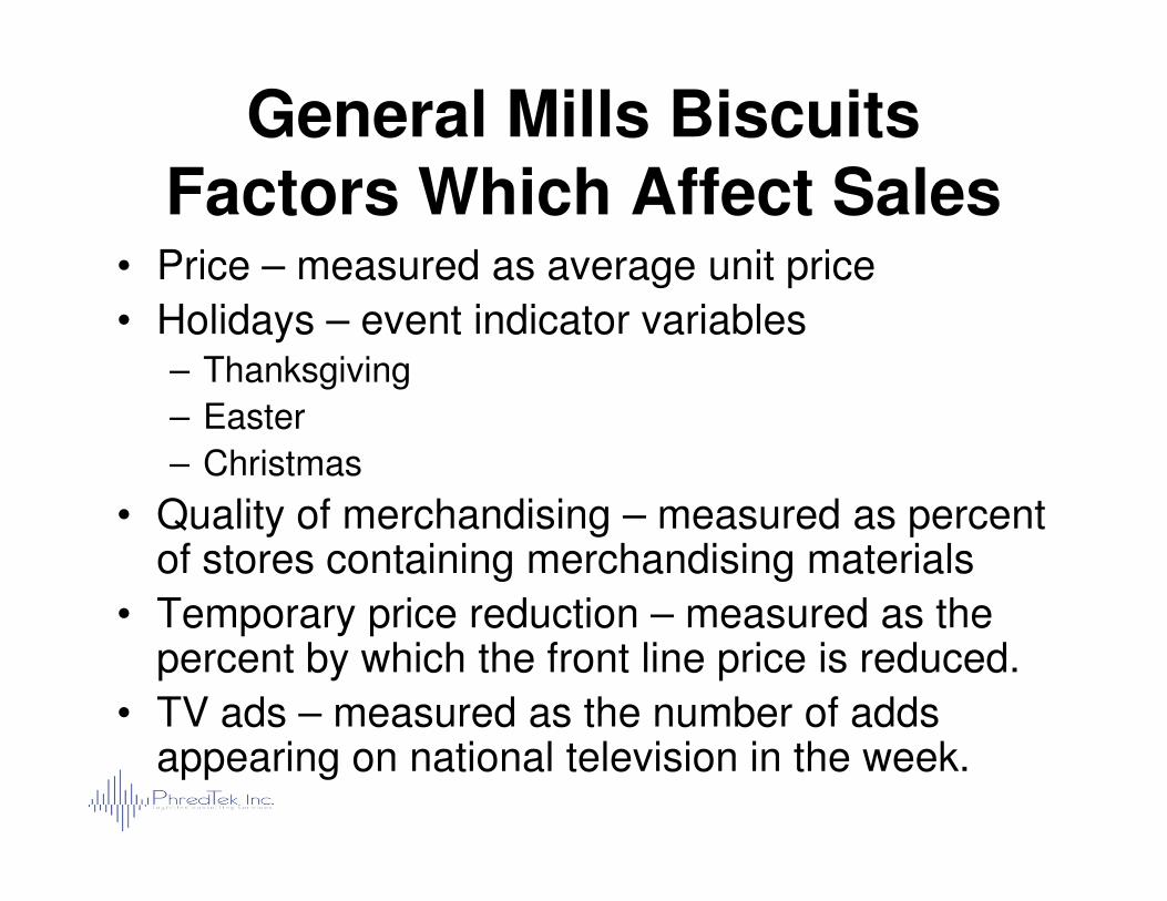
General Mills Biscuits Factors Which Affect Sales
• Price – measured as average unit price
• Holidays – event indicator variables– Thanksgiving
– Easter
– Christmas– Christmas
• Quality of merchandising – measured as percent of stores containing merchandising materials
• Temporary price reduction – measured as the percent by which the front line price is reduced.
• TV ads – measured as the number of adds appearing on national television in the week.
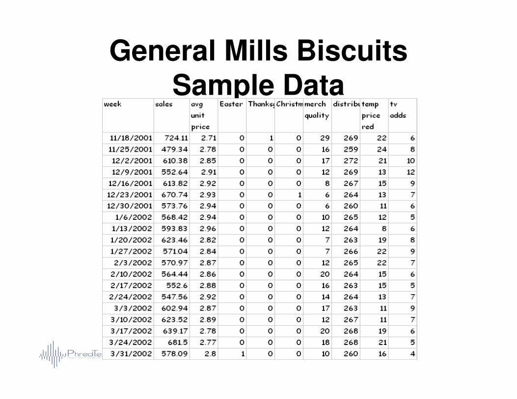
General Mills Biscuits Sample Data
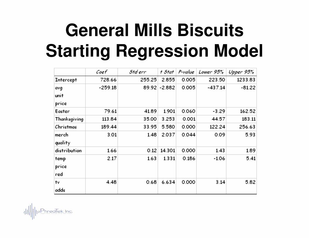
General Mills BiscuitsStarting Regression Model
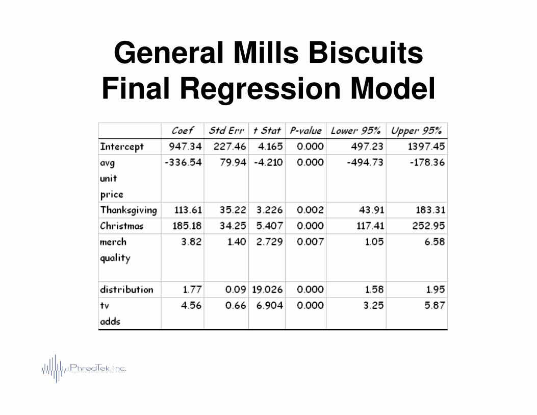
General Mills BiscuitsFinal Regression Model
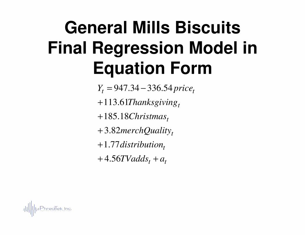
General Mills BiscuitsFinal Regression Model in
Equation Form
t
t
tt
Christmas
ngThanksgivi
priceY
+
+
−=
18.185
61.113
54.33634.947
tt
t
t
t
aTVadds
ondistributi
tymerchQuali
Christmas
++
+
+
+
56.4
77.1
82.3
18.185
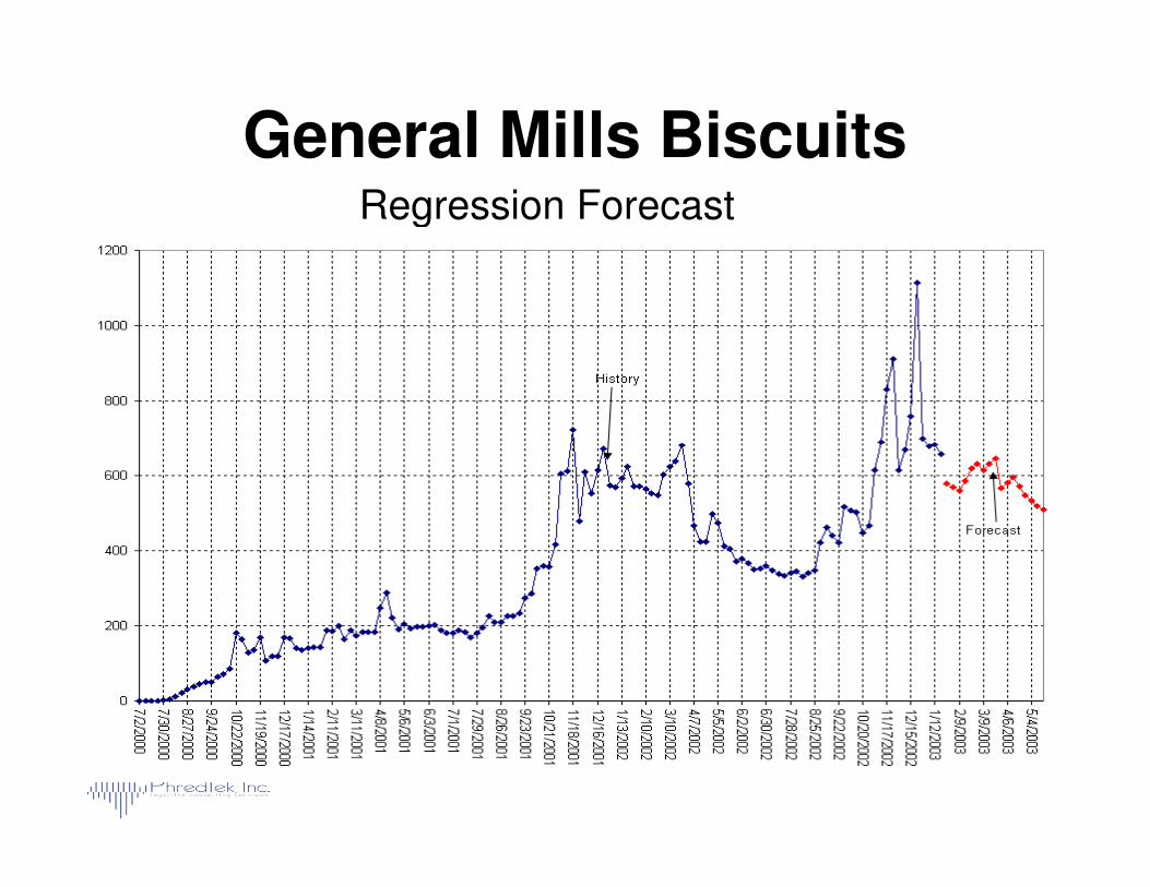
General Mills BiscuitsRegression Forecast
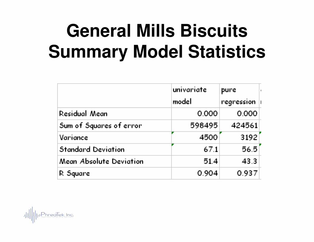
General Mills BiscuitsSummary Model Statistics
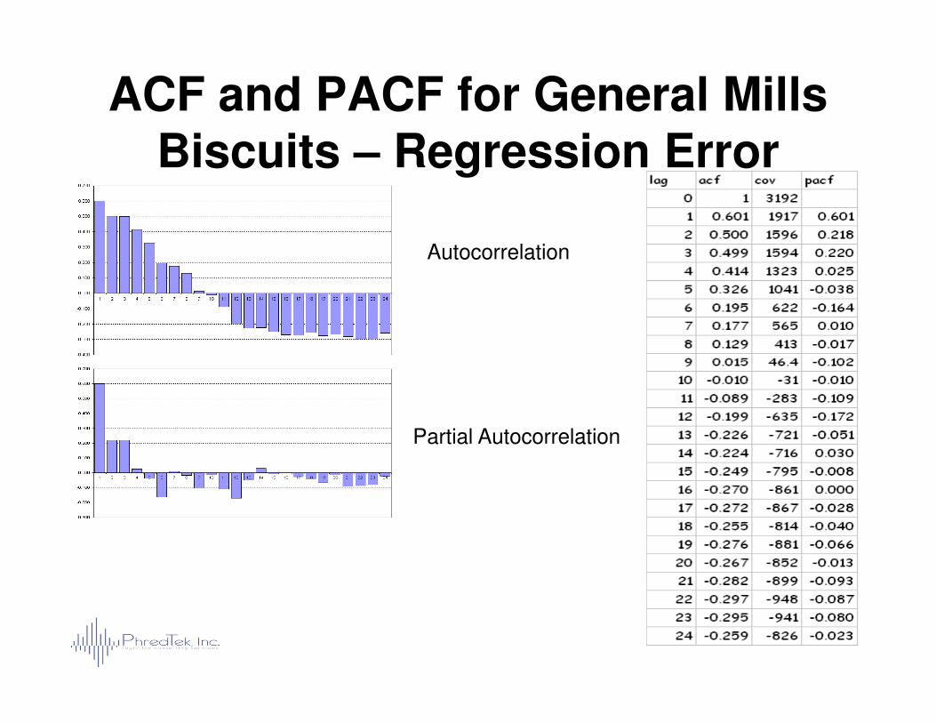
ACF and PACF for General Mills Biscuits – Regression Error
Autocorrelation
Partial Autocorrelation
General Mills Biscuits Problems with the regression model
• Autocorrelation is significant– Violates the regression assumption that errors
are not correlated
– Places the entire result in question.
• It does not consider potential lead and lag effects on causal variables.
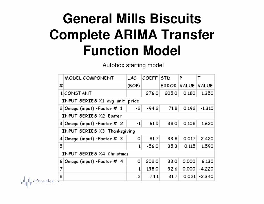
General Mills BiscuitsComplete ARIMA Transfer
Function ModelAutobox starting model
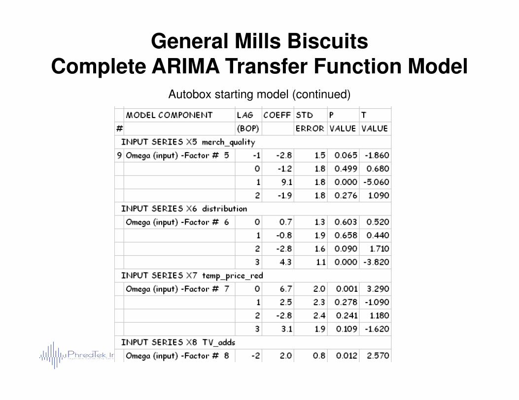
General Mills BiscuitsComplete ARIMA Transfer Function Model
Autobox starting model (continued)
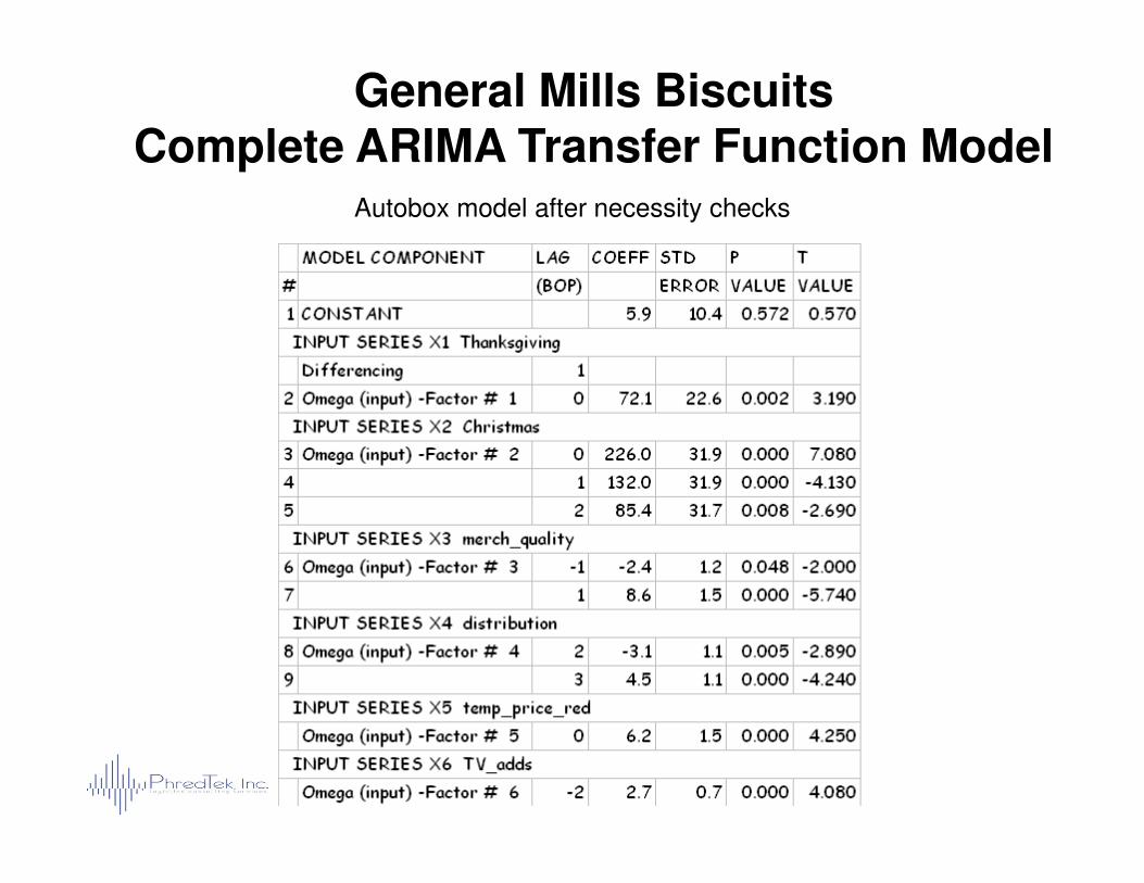
General Mills BiscuitsComplete ARIMA Transfer Function Model
Autobox model after necessity checks
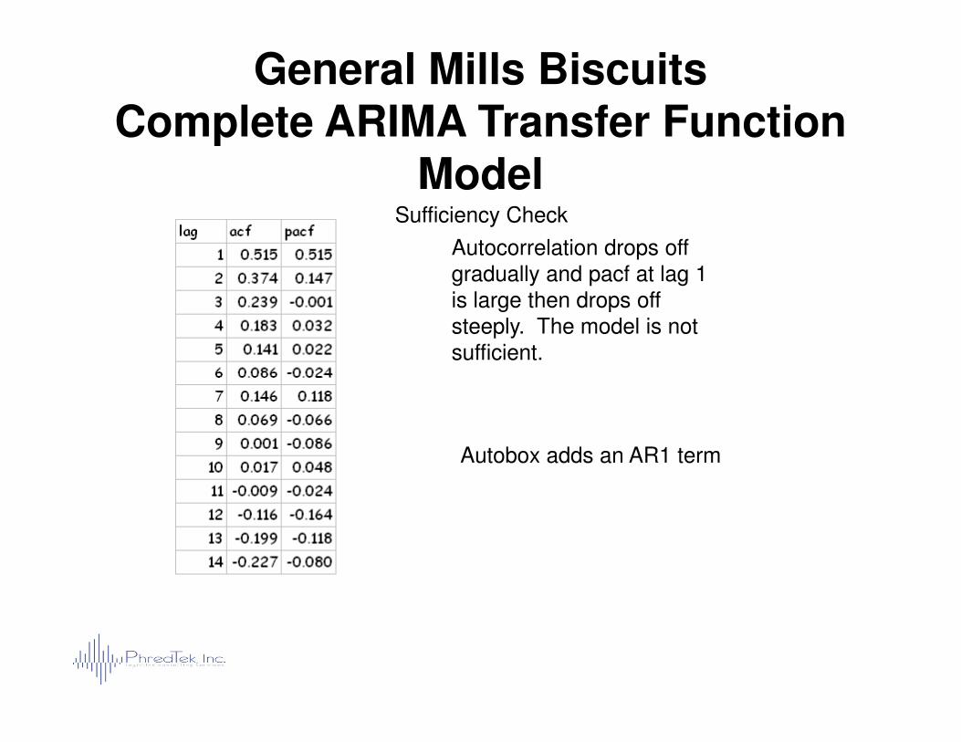
Autocorrelation drops off gradually and pacf at lag 1 is large then drops off steeply. The model is not sufficient.
General Mills BiscuitsComplete ARIMA Transfer Function
ModelSufficiency Check
Autobox adds an AR1 term
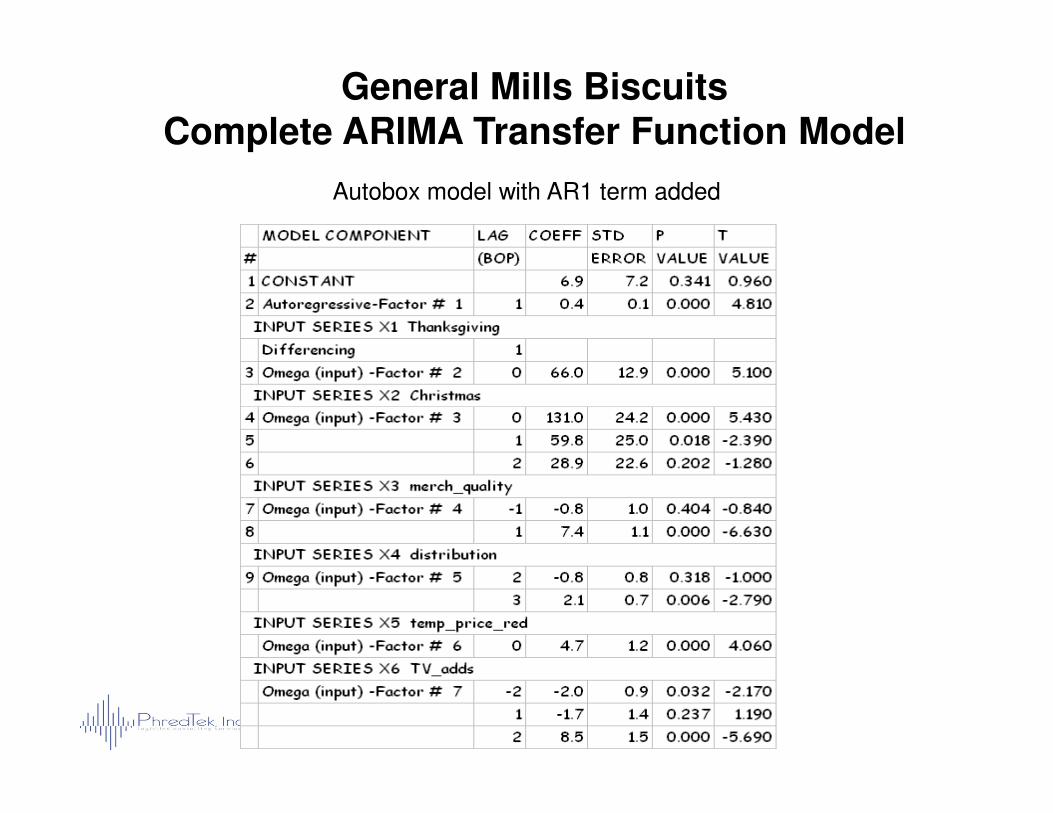
General Mills BiscuitsComplete ARIMA Transfer Function Model
Autobox model with AR1 term added
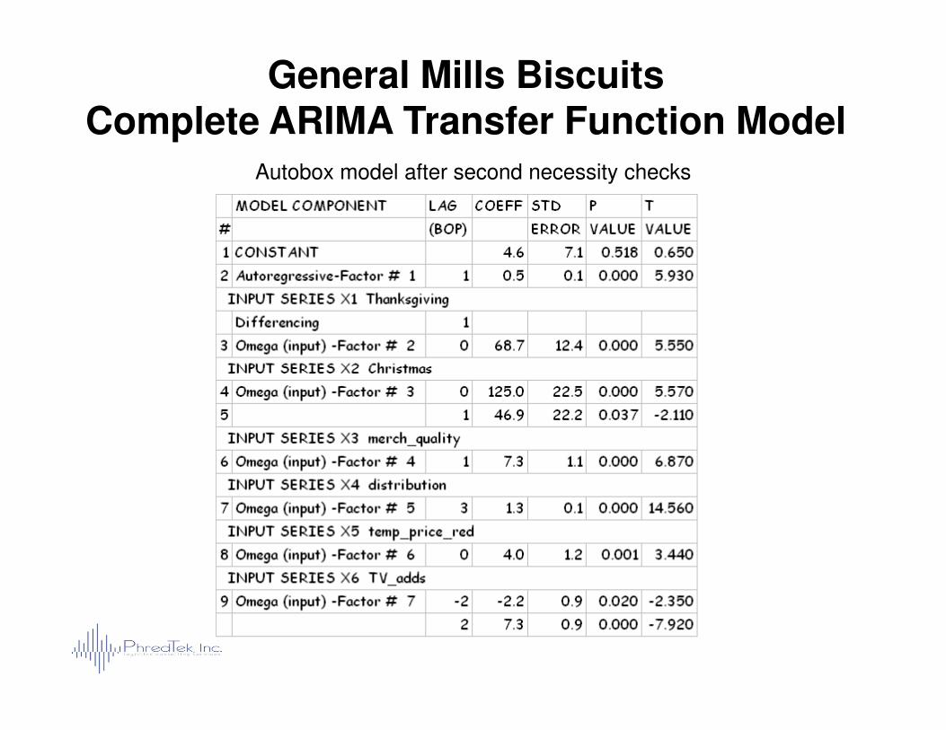
General Mills BiscuitsComplete ARIMA Transfer Function Model
Autobox model after second necessity checks
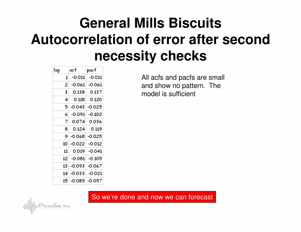
General Mills BiscuitsAutocorrelation of error after second
necessity checks
All acfs and pacfs are small and show no pattern. The model is sufficient
So we’re done and now we can forecast
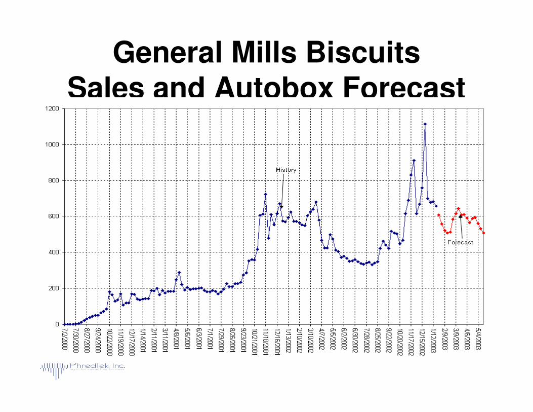
General Mills BiscuitsSales and Autobox Forecast
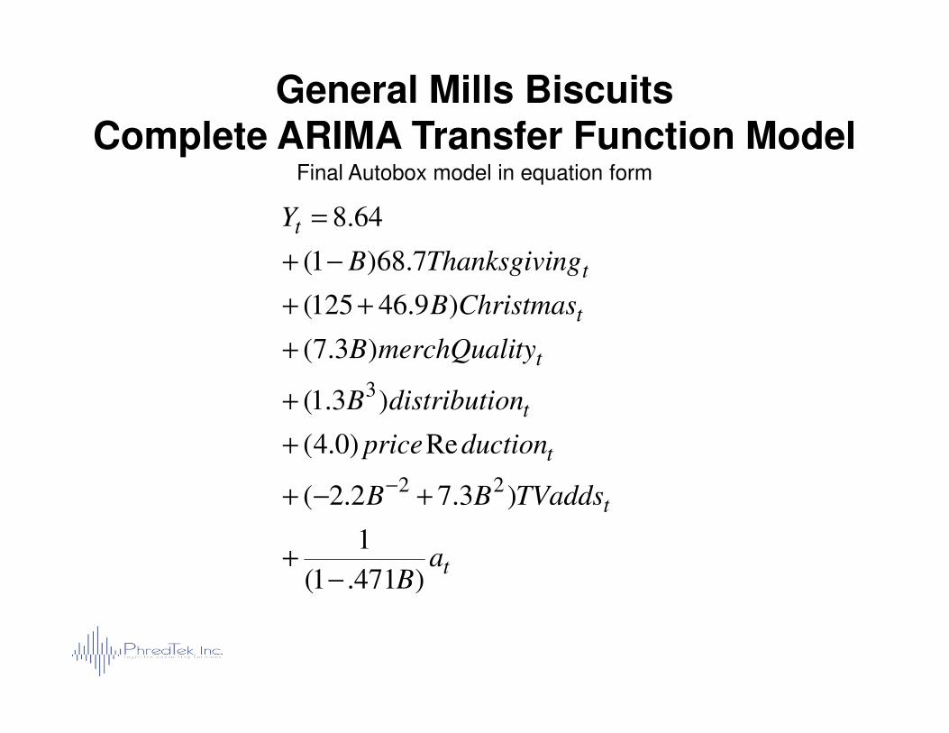
General Mills BiscuitsComplete ARIMA Transfer Function Model
Final Autobox model in equation form
t
t
t
t
tymerchQualiB
ChristmasB
ngThanksgiviB
Y
)3.7(
)9.46125(
7.68)1(
64.8
+
++
−+
=
t
t
t
t
t
aB
TVaddsBB
ductionprice
ondistributiB
)471.1(
1
)3.72.2(
Re)0.4(
)3.1(
22
3
−+
+−+
+
+
−
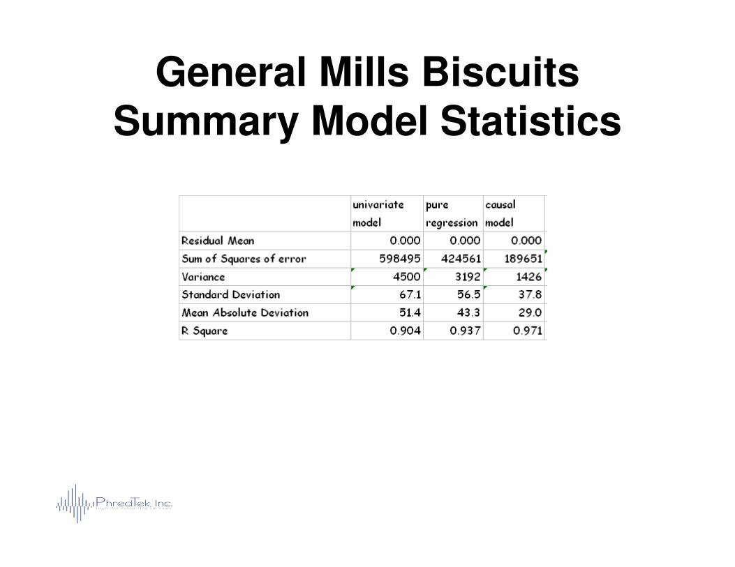
General Mills BiscuitsSummary Model Statistics
Outliers Types of Outliers
• One time outliers – called pulses
• Level shifts
• Outliers that repeat every season – called seasonal pulses
Outliers are called interventions in the literature
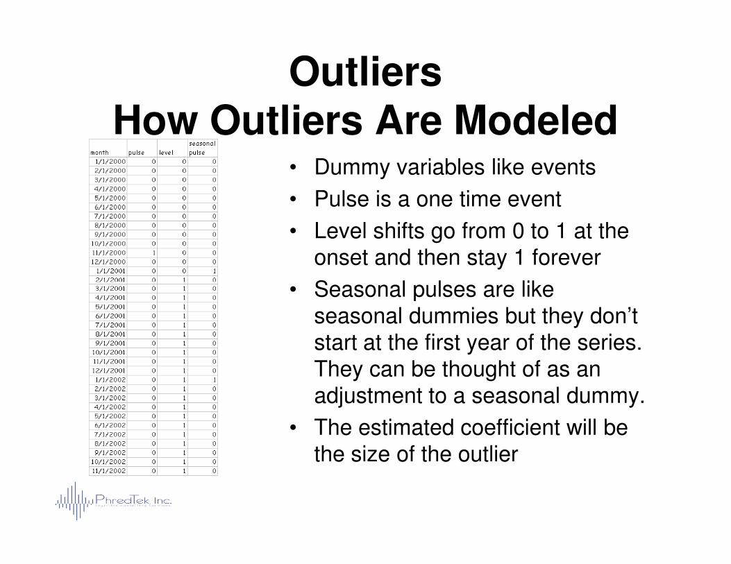
Outliers How Outliers Are Modeled
• Dummy variables like events
• Pulse is a one time event
• Level shifts go from 0 to 1 at the onset and then stay 1 forever
• Seasonal pulses are like • Seasonal pulses are like seasonal dummies but they don’t start at the first year of the series. They can be thought of as an adjustment to a seasonal dummy.
• The estimated coefficient will be the size of the outlier
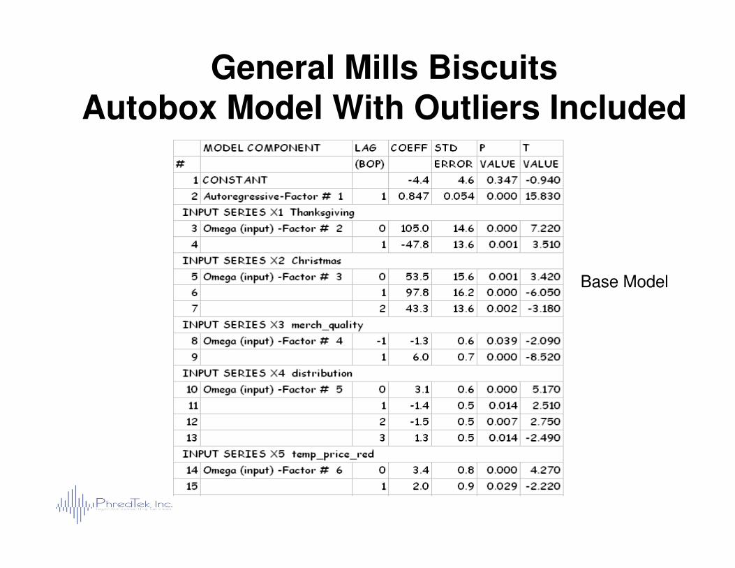
General Mills BiscuitsAutobox Model With Outliers Included
Base ModelBase Model
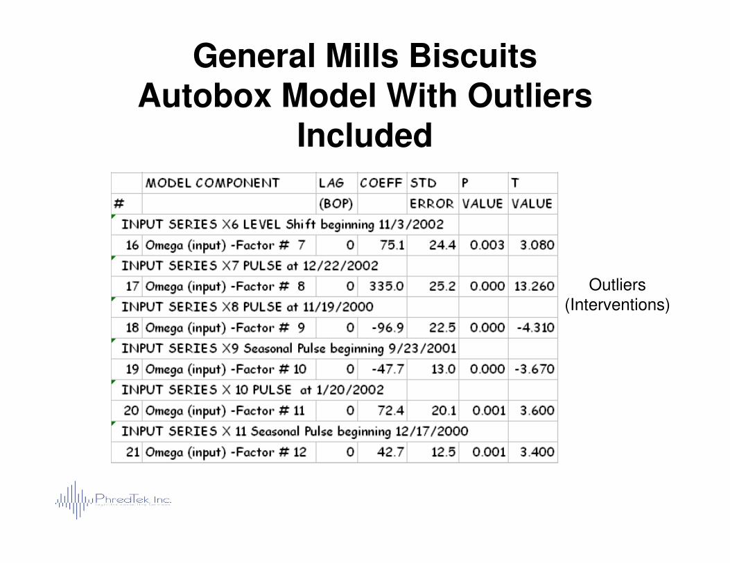
General Mills BiscuitsAutobox Model With Outliers
Included
Outliers Outliers (Interventions)
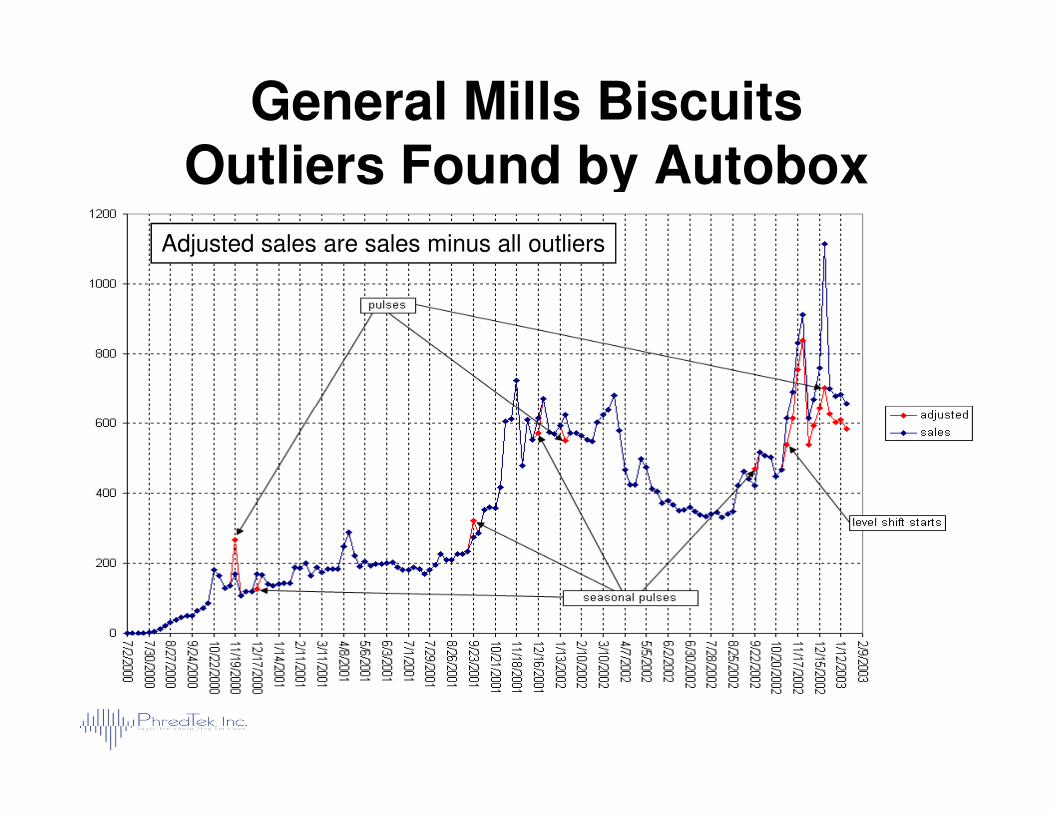
General Mills BiscuitsOutliers Found by Autobox
Adjusted sales are sales minus all outliers
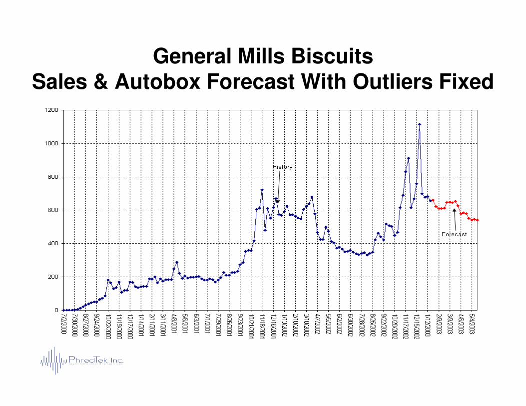
General Mills BiscuitsSales & Autobox Forecast With Outliers Fixed
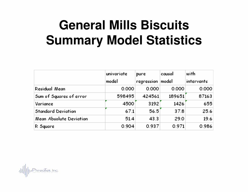
General Mills BiscuitsSummary Model Statistics

Beer Sales by Brand and Package at One Grocery
Store
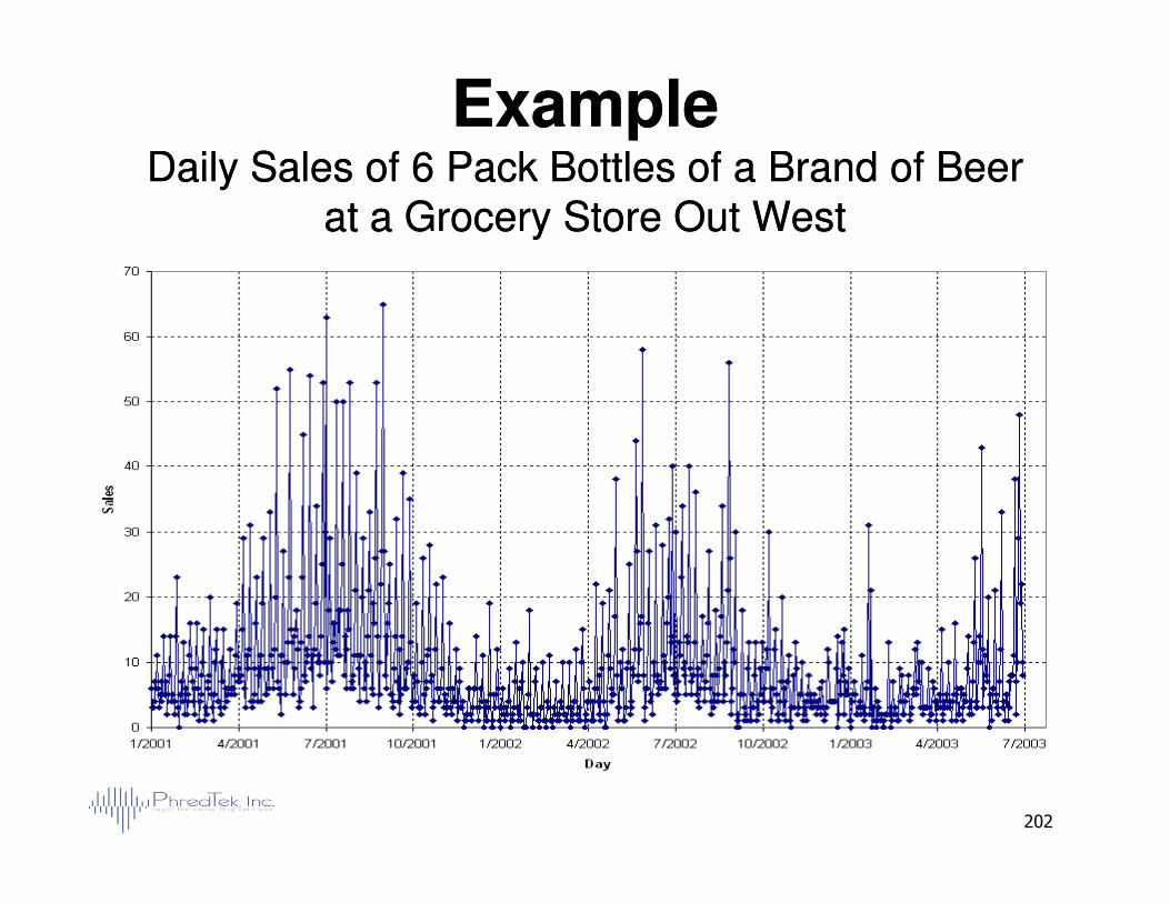
ExampleExampleDaily Sales of 6 Pack Bottles of a Brand of BeerDaily Sales of 6 Pack Bottles of a Brand of Beer
at a Grocery Store Out Westat a Grocery Store Out West
202
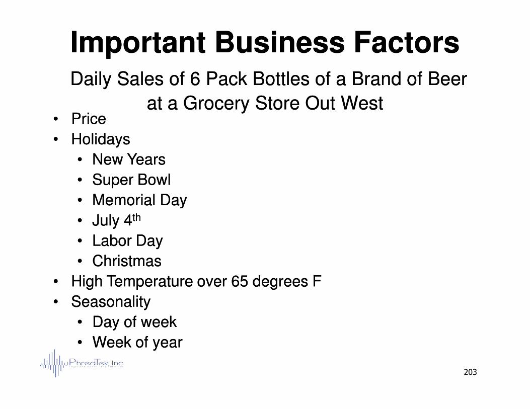
Important Business FactorsImportant Business FactorsDaily Sales of 6 Pack Bottles of a Brand of BeerDaily Sales of 6 Pack Bottles of a Brand of Beer
at a Grocery Store Out Westat a Grocery Store Out West•• PricePrice
•• HolidaysHolidays
•• New YearsNew Years
•• Super BowlSuper Bowl
•• Memorial DayMemorial Day
203
•• Memorial DayMemorial Day
•• July 4July 4thth
•• Labor DayLabor Day
•• ChristmasChristmas
•• High Temperature over 65 degrees FHigh Temperature over 65 degrees F
•• SeasonalitySeasonality
•• Day of weekDay of week
•• Week of yearWeek of year
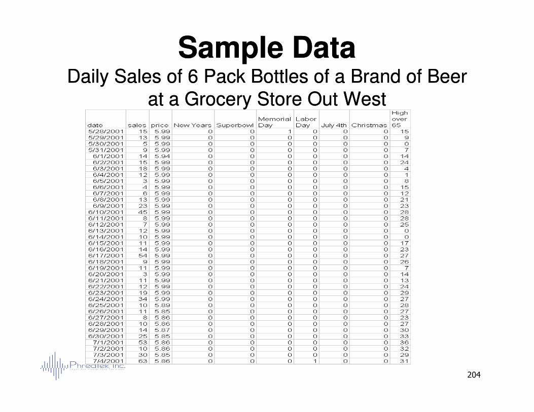
Sample DataSample DataDaily Sales of 6 Pack Bottles of a Brand of BeerDaily Sales of 6 Pack Bottles of a Brand of Beer
at a Grocery Store Out Westat a Grocery Store Out West
204
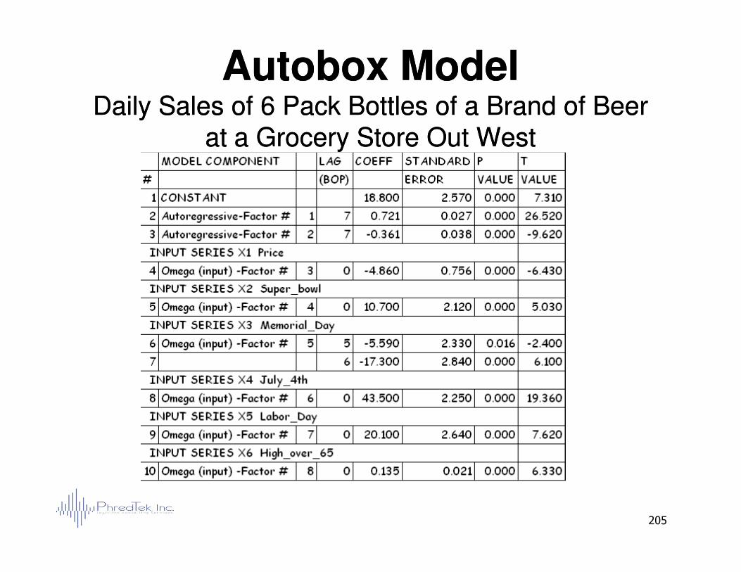
Autobox ModelAutobox ModelDaily Sales of 6 Pack Bottles of a Brand of BeerDaily Sales of 6 Pack Bottles of a Brand of Beer
at a Grocery Store Out Westat a Grocery Store Out West
205
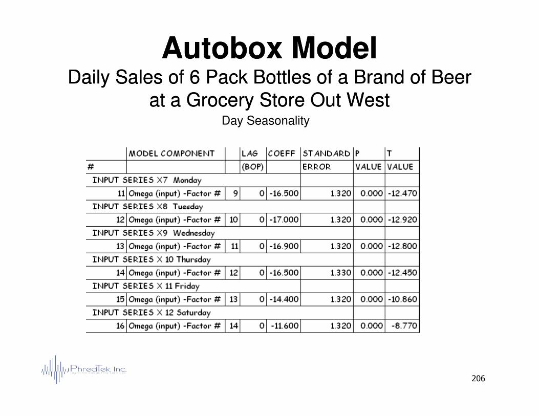
Autobox ModelAutobox ModelDaily Sales of 6 Pack Bottles of a Brand of BeerDaily Sales of 6 Pack Bottles of a Brand of Beer
at a Grocery Store Out Westat a Grocery Store Out WestDay Seasonality
206
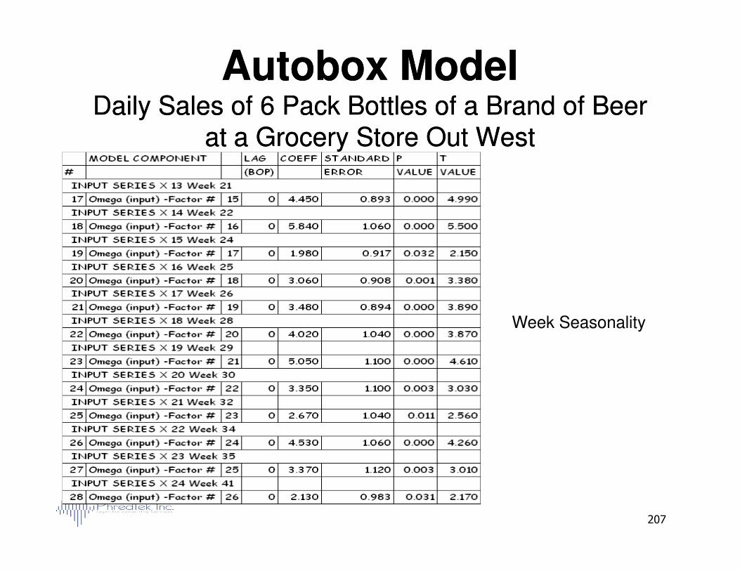
Autobox ModelAutobox ModelDaily Sales of 6 Pack Bottles of a Brand of BeerDaily Sales of 6 Pack Bottles of a Brand of Beer
at a Grocery Store Out Westat a Grocery Store Out West
207
Week Seasonality
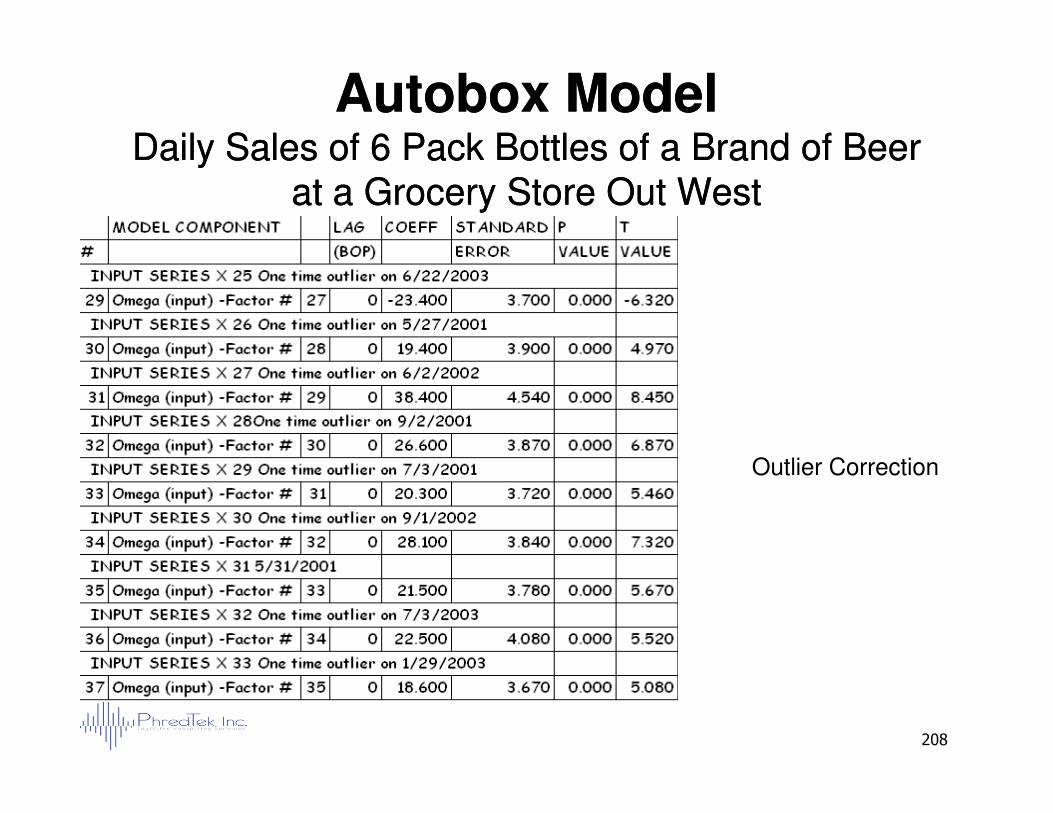
Autobox ModelAutobox ModelDaily Sales of 6 Pack Bottles of a Brand of BeerDaily Sales of 6 Pack Bottles of a Brand of Beer
at a Grocery Store Out Westat a Grocery Store Out West
208
Outlier Correction