Statistical Commission Background document

Fifty-third session Available in English only

1–4 March 2022

Item 3(s) and 3(u) of the provisional agenda

Items for discussion and decision: agricultural and rural statistics and big data

UNITED NATIONS United Nations Statistical Commission

United Nations Committee of Experts on Big Data and Data Science for Official Statistics (UN-CEBD)

Earth Observation Joint Task Team on Agricultural Production Statistics

Research Sub Task Team

Trusted methods: Lessons Learned and Recommendations from Select Earth Observation Applications on Agriculture

Presented by Maria Ximena Correa Olarte (DANE), Sara Burns (STATCAN), Lorenzo DeSimone (FAO), Talip Kilic (World bank), Michael Schmidt (DLR), Gordon Reichert (STATCAN),

2

Special Thank You to the peer reviewers who contributed meaningful commentary for the completion of the trusted methods report.

Andrew Robson, Precision Agriculture Research Group (PARG), University of New England, Australia

Saeid Homayouni, Associate Professor ; INRS Québec City, Canada Centre Eau Terre Environnement (ETE)

Mostafa Khorsandi, Student : Ph.D Candiate, INRS Québec City, Canada, Centre Eau Terre Environnement (ETE)

Further Thank You for the support from the Earth Observation Joint Task Team on Agricultural Production Statistics Research Sub Task Team and the associated Steering Committee.

3

Table of contents Table of Figures .................................................................................................................... 4

Tables ................................................................................................................................... 5

Executive summary ............................................................................................................... 6

Background ........................................................................................................................... 8

Use cases ............................................................................................................................. 9

Large area operational multi-season, multi-sensor crop mapping Submitted by: DLR ........ 9

EOSTAT LESOTHO Submitted by: FAO ...........................................................................19

EOSTAT SENEGAL Submitted by: FAO ...........................................................................28

Improvement of land cover classification process using Machine Learning in cloud computing from Sentinel-2 satellite images with RPAS image injection. Submitted by: National Administrative Department of Statistics (DANE) ..................................................49

Earth Observation data analytics for Greenhouse detection and production area estimation Submitted by: Statistics Canada .......................................................................................57

Understanding the Requirements for Surveys to Support Satellite-Based Crop Type Mapping: Evidence from Sub-Saharan Africa Submitted by: World Bank ..........................63

Final recommendations and lessons learned ........................................................................73

Terminology .........................................................................................................................79

References ...........................................................................................................................90

4

Table of Figures

Figure 1. Location of study area. ..........................................................................................10 Figure 2. Time-series modelling. ..........................................................................................12 Figure 3. Configuration of the tiered, tree-based classification model. ..................................14 Figure 4. Exemplar EVI time-series. .....................................................................................15 Figure 5. Predicted groups. ..................................................................................................16 Figure 6. Lesotho Land Cover Atlas, FAO 2015. ..................................................................19 Figure 7. Overview of the new land cover production methodology applied for Lesotho. .......21 Figure 8. Mine site as classified in the LC 2015 ....................................................................21 Figure 9. Results of K-mean performed within a “mine” class object .....................................22 Figure 10. National Land Cover Map 2020 ...........................................................................24 Figure 11. Architecture implemented for the production of the 2020 Lesotho Land Cover Data .............................................................................................................................................26 Figure 12. Google Cloud Computing Costs entailed for the 2020 Lesotho Land Cover data production. ...........................................................................................................................26 Figure 13. Sentinel-2 tiles overlaid on Senegal Administrative units .....................................28 Figure 14. Household locations covered by the 2018 agricultural survey ..............................29 Figure 15. GPS tracks location (left) and parcels boundaries with GPS point/lines (right) .....30 Figure 16. GPS traces successfully converted in shapefiles and represented well parcels boundaries ...........................................................................................................................30 Figure 17. Example of GPS traces that contain more than parcels boundaries ....................31 Figure 18. Distribution of crop polygons areas according to the crop type ............................32 Figure 19. Challenge to localize the surveyed parcels in the statistical database due to the fact that parcels are localized by geo-points (i.e. a single GPS coordinate) .................................32 Figure 20. Interpretation of non-cropland information by visual interpretation of very high resolution imagery: Build up, water body, close forest ..........................................................33 Figure 21. Distribution of non-crop polygons superficies according to land cover .................34 Figure 22. Location of the 1,593 crop polygons obtained from the GPS boundaries .............36 Figure 23. Overview of the cropland mask (V1.0) at national scale.......................................36 Figure 24. Zooms of the cropland mask (V1.0) in the right column (black = non cropland) overlaid with Google Earth imagery (left column) ..................................................................38 Figure 25. Overview of the crop type map (V1.0) at national scale .......................................39 Figure 26. Zooms of the crop type map (V1.0) overlaid with Google Earth imagery ..............39 Figure 27. Distribution of non-crop polygons superficies according to land cover (V2.0) .......41 Figure 28. Localization of the 4,252 crop polygons and buffered points obtained from the GPS data base .............................................................................................................................41 Figure 29. Overview of the crop type map (V2.0) at national scale .......................................42 Figure 30. Comparison of the main crop types area obtained from EO data (blue) and as reported in the FAOSTAT (orange) (V2.0) ............................................................................46 Figure 31. UN Global Platform solution diagram for the EO-STAT project in Senegal ..........47 Figure 32. Location of study areas for DANE’s project. .........................................................50 Figure 33. Visual comparison among images. ......................................................................53 Figure 34. Classification visual comparison. .........................................................................53

5

Tables

Table 1. Observations of the groups .....................................................................................11 Table 2. Explanatory variables for the classification model. ..................................................13 Table 3. Error matrix for the summer-cropping phase, for validation data pooled over all growing seasons. .................................................................................................................15 Table 4. Error matrix for the winter-cropping phase, for validation data pooled over all growing seasons. ...............................................................................................................................16 Table 5. Confusion matrix of the Crop Type map (V1.0) .......................................................40 Table 6. Confusion matrix of the Crop Type map (V2.0) .......................................................42 Table 7. Cropland - non cropland area indicators at national and provincial level .................45 Table 8. Area indicators of the main crop types at national scale (V2.0) ...............................45 Table 9. Characteristics of the Sentinel-2 images collection. ................................................50 Table 10. Characteristics of RPAS images. ..........................................................................51 Table 11. Thematic quality synthesis. ...................................................................................54 Table 12. Satellites, bands and indices used in the analysis.................................................64 Table 13. Additional EO data used in the maize classification pipeline .................................66

6

Executive summary

Crop acreage, crop yield and crop productivity statistics are fundamental for the Countries’ monitoring of and reporting on the agricultural production system allowing them to plan its commodity value chains, and to formulate efficient policies that ensure food security.

As more pressure is exerted on food systems globally, because of the compound effect of increased human population, climate change, and worsened Agri-environmental conditions, the National Statistics Offices (NSO’s) are faced with the need to produce timelier, frequent, and granular agricultural statistics. Such demand for higher efficiency can be met using Big Data, Open source technology, artificial intelligence and Earth Observations (EO) data. Earth observation data can facilitate such monitoring and reporting processes, thanks to their intrinsic characteristics of spatial extensive coverage, high spatial, spectral, and temporal resolution, and low costs1. This is done in order to reduce the frequency and the dimensions of surveys, to reduce respondent burden and other costs and to provide data at a more disaggregated level for informed decision making.

The UN General Assembly2 had early recognized in 2015 the key transformational role of EO data in support of countries reporting duties under the SDG framework. This was further reflected in the establishment of several EO coordination bodies such as the Group on Earth Observations (GEO), the United Nations Committee of Experts on Global Geospatial Information Management (UN-GGIM), and a series of UN Working groups.

It is within such context that the UN Nations Statistical Commission and the UN Department of Economic and Social Affairs (UNDESA), are working to support NSO’s worldwide in the uptake of EO data within their statistical workflows under the broad scope of the modernization process of statistical systems.

To this end, the Task Team (TT) of the UN Committee of Experts on Big Data and Data Science for Official Statistics was established in 2014 under the coordination of the UNDESA, with the scope of providing strategic vision, direction, and development of a global work plan on utilising satellite imagery and geo-spatial data for official statistics and indicators for post-2015 development goals.

The work of the TT includes supporting countries through the:

• Identification of reliable and accurate statistical methods for estimating quantities of interest;

• Suggestion of approaches for collecting representative training and validation data of sufficient quality;

• Research, develop and implement assessment methods for the proposed models including measures of accuracy and goodness of fit;

• Establishing strategies to reuse and adapt algorithms across topics and to build implementations for large volumes of data.

Since the establishment of the TT, several statistical agencies worldwide have shown a strong interest in investigating the viability of using satellite imagery to extract official statistics on

1 L.Desimone et Al., 2021 2 United Nations General Assembly. Transforming Our World: The 2030 Agenda for Sustainable Development; United Nations: New York, NY, USA, 2015.

7

agriculture as well as on environmental resources. As a result, a series of pilot projects have been implemented using a variety of methods and approaches.

For example, the Government of Australia has used a blended time series of low, medium and high-resolution satellite images combined with a supervised classifier (Random Forest) to identify actively growing crops in the Queensland region. The Ministry of Agriculture in Senegal, in collaboration with FAO, has relied on high resolution images (Sentinel2) to assess retrospectively crop acreage for the year 2018 using the Sen2Agri toolbox developed by the European Space Agency. The Government of Lesotho, supported by FAO, is using Sentinel-2 data to produce annual land cover maps and establish a national time series of standardized land cover maps for the period 2017-2022. Furthermore, the Geostatistical Development and Research Unit of the Geostatistics Directorate of the Colombian National Statistical Office has improved the national land cover classification process using Machine Learning in cloud computing from Sentinel-2 satellite images fused with very-high resolution RPAS images, which come at sub-meter pixel size.

This handbook, written by members of the Task Team of the UN Committee of Experts on Big Data and Data Science for Official Statistics, provides an overview of the above-mentioned use cases, illustrating the methods, the lessons learned, and the results and recommendations.

The handbook aims to expose the key steps faced along the production-chain for deriving EO-based statistics and explain how these have been handled in selected national use cases.

Such key steps can be summarised as:

i) the EO data and pre-processing, ii) the In-situ data gathering and QA/QC iii) methodology iv) classification algorithm.

For each national use case a results and recommendations paragraph has been addressed for final reflections.

8

Background

The use of Earth Observation (EO) data for the generation of official statistics has been recognized by the United Nations (UN) Statistical Commission as one of the cornerstones of the statistical modernization process in relation to the use of Big Data as an alternative and/or integrative source of information to traditional censuses and surveys (Task Team on Using Big Data for the Sustainable Development Goals — UN-CEBD). The recent report of the Independent Expert Advisory Group (IEAG) on the Data Revolution for Sustainable Development states that statistical agencies should choose data sources with regard to quality, timeliness, costs, and response burden, and Big Data sources fall within this scope. To monitor certain indicators Big Data could have the potential to be as relevant, more timely, and more cost effective than traditional data collection methods, and could make the data cycle match the decision cycle. The work on Big Data should contribute to the adoption of best practices for improving the monitoring of the new SDGs under the Post-2015 development agenda. Some of the new indicators or proxies of those indicators could be based on Big Data sources with improved timeliness and granular social and geo-spatial breakdown.

This is consistent with the Decision of the 45th session of the Statistical Commission in 2014, which recognized that Big Data constitutes a source of information that cannot be ignored. To achieve this, the Commission created a UN Committee of Experts on Big Data and Data Science for Official Statistics to explore the use of Big Data, identify examples, assess methodologies, address concerns related to quality and confidentiality, and develop guidelines.

A Task Team on Satellite Imagery was first created in 2014 (under the Global Working Group on Big Data for Official Statistics), with a mandate to identify approaches for collecting representative training data; and develop and implement methods using satellite imagery and the training data for producing official statistics, including the statistical application of predictive models for crop production yields. The task team was later renamed to the Task Team on Earth Observation Data for Agriculture Statistics to not limit the data sources just to satellite imagery.

The main objective of the Task Team is to provide concrete examples of the potential use of EO data for official statistics. This means, in particular, TT to develop and share methods for estimating crop location, crop type and crop yield using optical data, and to produce global land cover and land use statistics. In 2017 a “Satellite Imagery and Geospatial Data Task Team report” was published as a handbook providing an introduction to the use of EO data for official statistics, types of sources available and methodologies for producing statistics from this type of data (UNGWG_Satellite_Task_Team_Report_WhiteCover.pdf).

The goal of this report by the research Sub-TT is to collate examples of recent EO applications with a particular focus on field data required to train and validate the respective methods used three representative case studies with up-to-date methodologies.

Members of the research Sub-TT are: Sara Burns (STATCAN), Gordon Reichert (STATCAN), Lorenzo DeSimone (FAO), Maria Ximena Correa Olarte (DANE), Talip Kilic (Worldbank), Michael Schmidt, Sean Lovell (UN)

9

Use cases Large area operational multi-season, multi-sensor crop mapping Submitted by: DLR 1. Project background

Managing land resources to support the needs of the population is a mandate common to all levels of government in Australia. This study by the Queensland Department of Science and Environment (QDES) used satellite imagery data to identify actively growing crops in Queensland, Australia. For the major broadacre cropping regions of Queensland the complete Landsat, Sentinel-2, and as a backup option, the Moderate Resolution Imaging Spectroradiometer (MODIS) archive from 1987 to 2018 was used in a multi-temporal mapping approach, where spatial, spectral and temporal information were combined in crop-modelling process, supported by training data sampled across space and time.

In this study, automated classification results were compared with data sources form official statistics.

2. Study area

The western cropping region of Queensland covers approximately 300,000 km2 (Figure 1). In general terms, rainfall in the study region is summer-dominant, and the soil has a large water-holding capacity; a combination that means that, in addition to summer-growing crops, it is possible to grow winter crops on stored soil moisture. The summer-cropping phase was defined as November to May, and the winter-cropping phase as June to October. The ‘growing season’ was referred to as a particular phase combined with a particular year, e.g. ‘Summer 1993’. The year of a summer-phase crop relates to the year in January. The major crops for the study region, and their grouping, are shown in Table 1. An amalgamation of ‘Coarse-grain’

10

and ‘Pulse’ into a single summer group was a pragmatic response to preliminary analyses that revealed strong confusion between the two, due to few observed summer-growing legumes.

Figure 1. Location of study area.

3. EO data / preprocessing

For efficiency, most of the satellite imagery used were found at the spacetime intersection of a single World Reference System-2 (WRS-2) Landsat scene and a single growing season, the study region spatially intersected 26 WRS-2 scenes.

Imagery were gathered for each growing season between the winter of 1987 and the winter of 2017, from, when available, the Landsat, Sentinel-2A, and MODIS satellites. Landsat imagery was pre-processed to surface reflectance (Flood et al., 2013). Sentinel-2A imagery was preprocessed to Landsat-like surface reflectance (Flood, 2017). MODIS imagery was obtained in the form of the MOD13Q1 product. Undesirable effects in any image—e.g. cloud contamination or open water—were masked.

Sentinel-2A and MODIS imagery were reprojected onto the grid of Universal Transverse Mercator pixel coordinates of the Landsat imagery. The geometric misregistration between Landsat-8 and Sentinel-2A rarely exceeded 15 m, which we regarded as satisfactory for this purpose (Pringle et al, 2018).

4. In situ data

Observations of the groups of Table 1 came from two sources. The first was an archive of 6,605 field observations collected between 1991 and 2017, evenly spread between summer and winter phases. This source was collected through a combination of roadside observation,

11

interviews with landholders, and desktop interpretation. The methods for collecting the roadside and interview observations were described by Pringle et al. (2012).

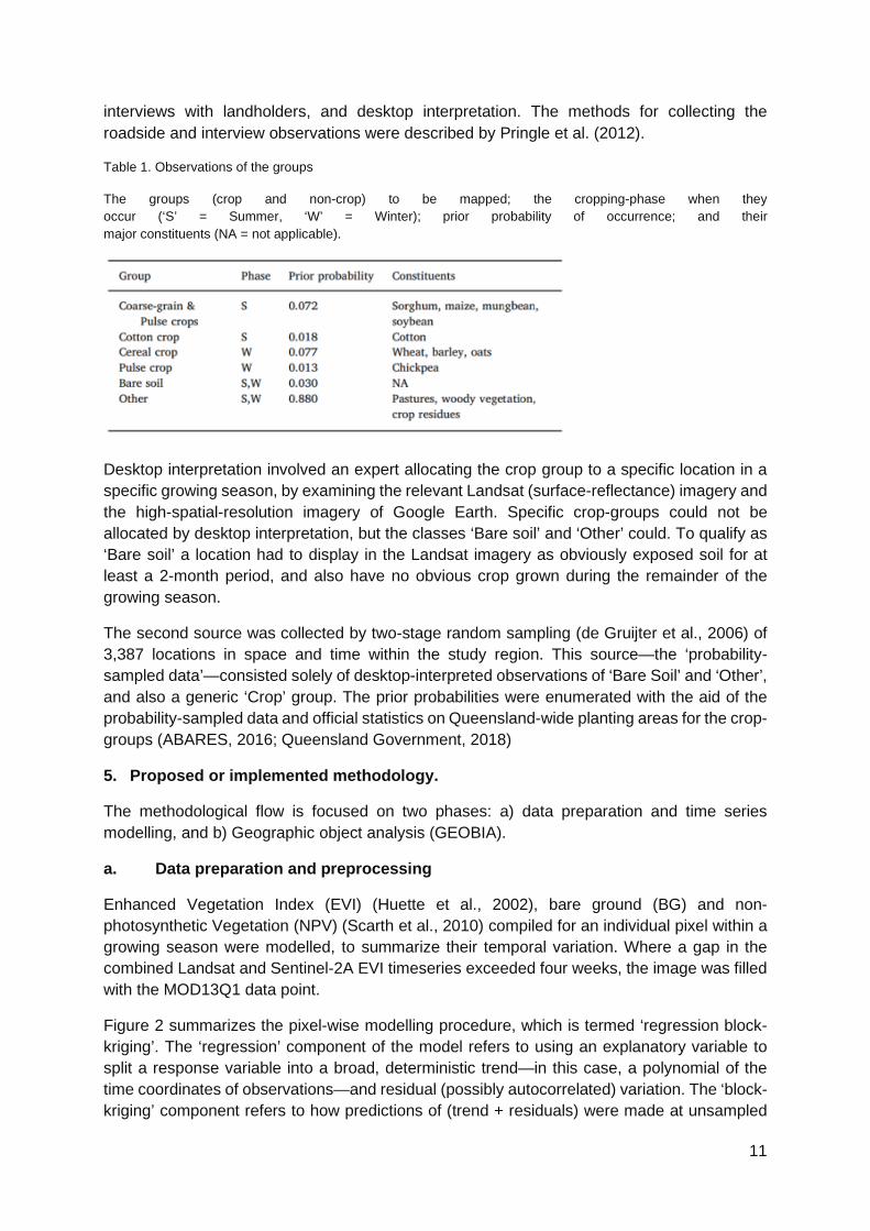
Table 1. Observations of the groups

The groups (crop and non-crop) to be mapped; the cropping-phase when they occur (‘S’ = Summer, ‘W’ = Winter); prior probability of occurrence; and their major constituents (NA = not applicable).

Desktop interpretation involved an expert allocating the crop group to a specific location in a specific growing season, by examining the relevant Landsat (surface-reflectance) imagery and the high-spatial-resolution imagery of Google Earth. Specific crop-groups could not be allocated by desktop interpretation, but the classes ‘Bare soil’ and ‘Other’ could. To qualify as ‘Bare soil’ a location had to display in the Landsat imagery as obviously exposed soil for at least a 2-month period, and also have no obvious crop grown during the remainder of the growing season.

The second source was collected by two-stage random sampling (de Gruijter et al., 2006) of 3,387 locations in space and time within the study region. This source—the ‘probability-sampled data’—consisted solely of desktop-interpreted observations of ‘Bare Soil’ and ‘Other’, and also a generic ‘Crop’ group. The prior probabilities were enumerated with the aid of the probability-sampled data and official statistics on Queensland-wide planting areas for the crop-groups (ABARES, 2016; Queensland Government, 2018)

5. Proposed or implemented methodology.

The methodological flow is focused on two phases: a) data preparation and time series modelling, and b) Geographic object analysis (GEOBIA).

a. Data preparation and preprocessing

Enhanced Vegetation Index (EVI) (Huette et al., 2002), bare ground (BG) and non-photosynthetic Vegetation (NPV) (Scarth et al., 2010) compiled for an individual pixel within a growing season were modelled, to summarize their temporal variation. Where a gap in the combined Landsat and Sentinel-2A EVI timeseries exceeded four weeks, the image was filled with the MOD13Q1 data point.

Figure 2 summarizes the pixel-wise modelling procedure, which is termed ‘regression block-kriging’. The ‘regression’ component of the model refers to using an explanatory variable to split a response variable into a broad, deterministic trend—in this case, a polynomial of the time coordinates of observations—and residual (possibly autocorrelated) variation. The ‘block-kriging’ component refers to how predictions of (trend + residuals) were made at unsampled

12

time locations, averaged over an aggregated interval, i.e. one week (see Pringle et al, 2018 for more details).

Figure 2. Time-series modelling.

(a) observations and the fitted polynomial trend; (b) two variograms for the residuals of the trend (dotted black lines are the parameter values c1 and d for the best of the authorised functions, in this case for Dowd's robust estimator); and (c) weekly predictions obtained through block-kriging of (trend + residuals). The influence of the outlying

13

observation in (a) is minimised by using the robust variogram, and subsequent winsorising and block-kriging. The ticks on the x-axis of (a) and (c) mark the extent of the growing season (Pringle et al., 2018)

Various phenological metrics of EVI, BG, and NPV were predicted as weekly averages for the duration of a growing season. For EVI the predicted maximum and the week of its occurrence were recorded. Table 2 lists the other metrics recorded.

Table 2. Explanatory variables for the classification model.

b. Processing GEOBIA

GEOBIA was used to obtain an approximation of field boundaries. This was necessary because Queensland has no publicly available information on sub-property fencing, and field boundaries can change between growing seasons, particularly where cropping is opportunistic. The image-segmentation module of the RSGISLib software (Bunting et al., 2014), was used. Unique segments are generated, i.e. a spatially contiguous cluster of pixels that is relatively homogeneous, conditional on the input image and the algorithm's driving parameters (Clewley et al., 2014).

The input image comprised three layers of pixel-wise time-series metrics: maximum weekly EVI, maximum weekly BG, and maximum weekly NPV. These layers formed a synthetic composite (Zhu et al., 2015), chosen to maximize discrimination between ‘fields’ that might, or might not, be cropped during the particular growing season. The minimum segment size was set to 25 Landsat pixels (2.25 ha).

Pixels that fell on roads, railways, stock routes, or an irrelevant land-use were masked prior to segmentation. Land-use in Queensland was baseline-mapped in 1999, and is updated occasionally on a per-catchment basis (Queensland Government, 2018). Relevant land-use classes for this study were: grazing of native vegetation or modified pastures; cropping; seasonal horticulture; and land-in-transition (ABARES, 2016). Temporal change in land-use was considered by choosing the closest contemporary land-use map to each growing season. Roads, railways and stock routes were considered temporally static.

6. Classification algorithm

The intersecting GEOBIA image-segment in space-time were matched to the observation with the corresponding values of explanatory variables.

The gathered data were split into training and validation subsets. For the crop-groups, the validation subset was drawn randomly from the observed data, with a constraint that the subset honour the frequency of ‘Crop’ in the probability sampled data.

14

Figure 3. Configuration of the tiered, tree-based classification model.

The form of the classification model was a tiered tree, comprising sub-models of two expert-elicited rules and two random forests (see Figure 3). The first expert rule, at the top of the tree, was for situations where the only group that could reasonably be expected was ‘Other’. The second expert rule prevented duplicated predictions of ‘Crop’, which arose when a time-series belonging to one growing season crossed substantially into the next. The threshold of bgMax < 0.52 was determined with the aid of a classification tree. The random forests were fitted with the randomForest library (Liaw and Wiener, 2002) of the R statistical software (R Core Team, 2016).

Predictions at the validation locations in space-time were obtained in the form of probabilities. The predicted probabilities of Random Forest 2 were multiplied by the predicted probability of ‘Crop’ for Random Forest 1, to create conditional outcomes. At a single validation location in space-time, the predicted group was chosen as the one with largest probability (i.e. plurality).

The overall agreement of observed groups with predicted groups in an error matrix was assessed with τp (Ma and Redmond, 1995), a modified form of the commonly used index-of-agreement.

15

7. Results & Recommendations

Figure 4 shows the time-series fitting for an image segment at a given location.

Figure 4. Exemplar EVI time-series. Satellite observations are shown as points. The dotted line is the fit of the polynomial trend. The solid line is the block-kriging prediction for the growing season, which accounts for any autocorrelation in the trend's residuals. Contemporary land-use is indicated above each panel.

When the classification model was applied at the space-time locations of all validation data, the error matrix for the summer-cropping phase suggested reasonable agreement between observed and predicted groups (Table 3, τp = 0.80). The threshold probability difference for reassigning a prediction of ‘Coarse-grain & Pulse’ to ‘Other’ was 0.55.

Table 3. Error matrix for the summer-cropping phase, for validation data pooled over all growing seasons. ‘CG&P’ is ‘Coarse-grain & Pulse’. ‘UA’ and ‘PA’ are user's and producer's accuracies, respectively. Prior probabilities for τp are given in Table 1. All values in brackets are the 95% confidence interval.

16

Table 4. Error matrix for the winter-cropping phase, for validation data pooled over all growing seasons. ‘UA’ and ‘PA’ are user's and producer's accuracies, respectively. All values in brackets are the 95% confidence interval.

Following this re-assignment the largest source of error was ‘Bare soil’ mistakenly predicted as ‘Other’. This error is due to the continuum of coexistence between bare soil and heavily grazed pastures, or bare soil and sparse crop residues. The error matrix for the winter-cropping phase also suggested reasonable agreement between observed and predicted groups (Table 4, τp = 0.86).

Figure 5. Predicted groups. The group predicted in each summer growing season for a 20-km × 20-km sub-region of Queensland. ‘CG&P’ represents ‘Coarse-grain & Pulse’.

From the perspective of a map-user, Table 3 and Table 4 indicate that, in any given growing season, we predicted ‘Coarse-grain & Pulse’ correctly in 79% of cases. The values for ‘Cotton’, ‘Cereal’ and ‘Pulse’ were 91%, 84%, and 73%, respectively. We predicted ‘Bare soil’ correctly in 72% of cases in summer, and 88% of cases in winter. When the validation data were broken into individual growing seasons, results for τp were consistent, except for poor showings in the summer of 1989, and the winter of 1992. The accuracy of the classification model fluctuated more in summer than in winter, which reflects the study region's summer-dominant, but highly variable, rainfall.

8. Solution Architecture

The computing hardware used was part of a high-performance computing cluster, comprising 6 nodes of 20 physical cores each, 1.29 TB of RAM in total, on Intel® Xeon® CPU E5-2680 v2 processors at 2.8 GHz, running the Linux SLES 11 (Service Pack 4) operating system

9. Bibliography

17

ABARES, Agricultural Commodity Statistics 2016. Australian Bureau of Agricultural and Resource Economics and Sciences, Canberra. Retrieved from www.agriculture.gov.au/abares/publications/display?url=http://143.188.17.20/anrdl/DAFFService/dis play.php%3Ffid%3Dpb_agcstd9abcc0022016_Sn9Dg.xml

Bunting, P., Clewley, D., Lucas, R.M., Gillingham, S., 2014. The remote sensing and GIS software library (RSGISLib). Comput. Geosci. 62, 216–226

Clewley, D., Bunting, P., Shephard, J., Gillingham, S., Flood, N., Dymond, J., Lucas, R., Armston, J., Moghaddam, M., 2014. A Python-based open source system for geographic object-based image analysis (GEOBIA) utilizing raster attribute tables. Remote Sens. 6, 6111–6135

Core Team, R., 2020. R: A Language and Environment for Statistical Computing. R Foundation for Statistical Computing, Vienna, Austria. www.R-project.org/ [Online; accessed 17-January-2022].

Flood, N., Danaher, T., Gill, T., Gillingham, S., 2013. An operational scheme for deriving standardised surface reflectance from Landsat

Flood, N., 2017. Comparing Sentinel-2A and Landsat 7 and 8 using surface reflectance over Australia. Remote Sens. 9, 659. de Gruijter, J., Brus, D., Bierkens, M., Knotters, M., 2006. Sampling for Natural Resource Monitoring. Springer, Berlin.

Frantz, D.; Roder, A.; Udelhoven, T.; Schmidt, M. Enhancing the Detectability of Clouds and Their Shadows in Multitemporal Dryland Landsat Imagery: Extending Fmask. IEEE Geosci. Remote Sens. Lett. 2015, 12, 1242–1246.

Government, Queensland, 2018. Agriculture: Area by Main Crop, Queensland, 2005–06 to 2015–16. www.qgso.qld.gov.au/products/tables/agriculture-area-main-crop-qld/index.php [Online; accessed 19-June-2018].

Huete, A., Didan, K., Miura, T., Rodriguez, E.P., Gao, X., Ferreira, L.G., 2002. Overview of the radiometric and biophysical performance of the MODIS vegetation indices. Remote Sens. Environ. 83, 195–213

Liaw, A., Wiener, M., 2002. Classification and regression by randomForest. R News 2 (3), 18–22. r-project.org/doc/Rnews/Rnews_2002-3.pdf [Online; accessed 17-January- 2022].

Ma, Z., Redmond, R.L., 1995. Tau coefficients for accuracy assessment of classification of remote sensing data. Photogramm. Eng. Remote Sens. 61, 435–439

Scarth, P., Röder, A., Schmidt, M., 2010. Tracking grazing pressure and climate interaction–the role of Landsat fractional cover in time series analysis. In: Proceedings of Australasian Remote Sensing and Photogrammetry Conference, Alice Springs, 13-17 September. figshare.com/articles/Tracking_Grazing_Pressure_and_Climate_ Interaction_-_The_Role_of_Landsat_Fractional_Cover_in_Time_Series_Analysis/ 94250/1

Schmidt, M., Pringle, M., Rakhesh, D., Denham, R. and D. Tindall. 2016. A Framework for Large-Area Mapping of Past and Present Cropping Activity Using Seasonal Landsat Images and Time Series Metrics https://doi.org/10.3390/rs8040312

18

Pringle, M.J., Denham, R.J., Devadas, R., 2012. Identification of cropping activity in central and southern Queensland, Australia, with the aid of MODIS MOD13Q1 imagery. Int. J. Appl. Earth Obs. Geoinf. 19, 276–285.

Pringle, M.J., Schmidt, M. and Tindall, D., 2018: Multi season, multi sensor time series modelling based on geostatistical concepts - to predict broad groups of crops. 216, p 183-200, DOI.org/10.1016/j.rse.2018.06.046

Zhu, Z., Woodcock, C.E., Holden, C., Yang, Z., 2015. Generating synthetic Landsat images based on all available Landsat data: predicting Landsat surface reflectance at any given time. Remote Sens. Environ. 162, 67–83.

19

EOSTAT LESOTHO Submitted by: FAO 1. Project background

The uptake of geospatial data products by NSO's as alternative data sources to produce official statistics depends on many factors, some of which are directly related to the availability of geospatial data that is accurate, granular, and regularly updated.

FAO developed the National Land Cover Atlas of Lesotho in 2015 jointly with the Ministry of Agriculture and Food Security (MAFS): such a product provided a foundation information layer for measuring the distribution of land cover across the country and extract land cover statistics at the subnational level. However, such Land Cover Atlas, resulting from a human driven visual interpretation of very high resolution images, resulted in very high production costs and time requirements, and as such it could not be updated on a regular basis. The product is now 7 years old.

In this context, in 2020 FAO launched the EOSTAT Lesotho project under the umbrella of the Integrated Catchment Management programme (ICM) funded by the multi donor consortium (EU, GIZ, Ministry of Lesotho), with the aim of i) developing a new methodology that allows for the production of annual national land cover maps, ii) to update the land cover atlas of Lesotho to the year 2020, and iii) to produce a time series of national land cover maps for the period 2016-2022.

The traditional method of land cover mapping used in the last two decades has been based on pixel classification or object classification and has relied typically on the use of very high-resolution images (Satellite images and orthophotos) and on in-situ data for calibration and validation. Such solutions have been extensively used in the research world (Cleve et al., 2008, Myint et al., 2011, Duro et al., 2012a, Tehrany et al., 2014). FAO adopted this approach in 2015 to deliver the first edition of the Lesotho Land Cover Atlas. This approach is resource intensive, requires a long time to deliver and is very difficult to automate.

With the advent of freely available high resolution satellite imagery, cloud computing facility and machine learning, it is now possible to carry out land cover mapping in a much more cost efficient way by integration of Machine Learning (ML) and Open Access Geospatial Data (Mardani, De Simone, 2019, Kim, Yeseul et al. 2017).

The development of the Lesotho land cover 2020 will directly benefit from such developments and will leverage the use of Satellite data (Sentinel-2) as well as the use of machine learning algorithms (Random forest), to train a classifier using class patterns from a previous Lesotho land cover database dated 2015.

As a result, the project will ensure reduced delivery time, reduced costs and high accuracy of deliverables.

The Lesotho Land Cover 2020 will constitute a foundation deliverable within the broader scope of the ICM monitoring project led by FAO. Allowing for the definition of baselines, and for the deeper monitoring of qualitative sub indicators of key ecosystems and land resources.

Figure 6. Lesotho Land Cover Atlas, FAO 2015.

20

The Lesotho Land Cover 2020 was produced alongside regional statistics in the same way as the Lesotho Land Cover 2015. The two products are difficult to compare due to the inherent difference between the methodologies, but the new semi-automated methodology implemented is promising in terms of output accuracy and cost-effectiveness.

In the context of the ICM project, production of the Land Cover product for the baseline year of 2016 (no Sentinel-2 data was available in 2015) should be considered for temporal inter-comparability, as well as a yearly product for the years 2017, 2018, 2019, and future years. This will enable the building of a fine-grained temporal picture of the evolution of land cover and the state of Lesotho’s key agricultural landscapes and ecosystems.

2. Study area Lesotho

3. EO data / preprocessing Google Earth Engine was used for the preprocessing of Sentinel-2 (S-2) data. S-2 tiles were acquired and transformed into an Analysis-Ready Data (ARD) cubes by performing temporal aggregation of the data over a time interval length of 60 days (2 months), which yielded 6 (almost) cloud-free temporal composites for the year 2020 (September 1st 2019-August 31st 2020). The tiles were first radiometrically normalized and cloud-masked. Subsequently the Max-NDVI temporal composites were produced. All of the 10m and 20m bands + NDVI + GLCM Correlation and Contrast of 10m bands were used as input features. As a final goal of the preprocessing, data size was reduced, only cloud-free observations at key phenological stages of the year were retained, and a time series data set sampled at regular intervals (2 months) was created. Error! Reference source not found., describes the entire workflow used to produce the national land cover (LC) map. In the red box the ARD component is

highlighted.

21

Figure 7 Overview of the new land cover production methodology applied for Lesotho.

(Red box highlights the ARD component)

4. In situ data At the time of the project, there was no availability of in-situ data gathered from previous survey work in the country. At the same time, it was not possible to deploy field data collection due to restrictions to movements imposed by the country in response to the Covid-19 Pandemic. In this context, the old land cover map (2015) was used to generate pseudo in-situ data using the methodology developed by Paris and Bruzzone (2021), but with the addition of some assumptions:

- The number of K-means clusters is fixed to 3 per class instead of using the Calinski-Harabasz Index to automatically determine the number of clusters. The assumption is that 3 clusters are enough to explain the within-class variance of each land cover classes, which were already selected for their prior probability of being homogeneous, i.e. selecting the “closed” classes and leaving out the “open” classes from the methodology.

- K-means clustering is performed per class and per agro-ecological zone for the entire area of interest rather than per polygon due to the small mean object size of the Lesotho Land Cover Data Base 2015 dataset. The minimum mapping unit (MMU) of 20m² (i.e. 1/5th of a sentinel-2 pixel) of the original land cover product is very small, and decomposing polygons using higher resolution imagery (in this case Sentinel-2) would not always lead to statistically meaningful clusters.

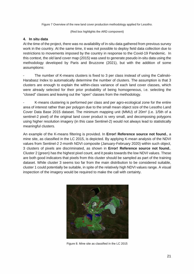
An example of the K-means filtering is provided. In Error! Reference source not found., a mine site, as classified in the LC 2015, is depicted. By applying K-mean analysis of the NDVI values from Sentinel-2 2-month NDVI composite (January-February 2020) within such object, 3 clusters of pixels are discriminated, as shown in Error! Reference source not found.. Cluster 2 (green) has the highest pixel count, and it peaks towards the low NDVI values. These are both good indicators that pixels from this cluster should be sampled as part of the training dataset. While cluster 3 seems too far from the main distribution to be considered suitable, cluster 1 could potentially be suitable, in spite of the relatively high NDVI values range. A visual inspection of the imagery would be required to make the call with certainty.

Figure 8. Mine site as classified in the LC 2015

22

Figure 9. Results of K-mean performed within a “mine” class object

The implementing steps required to generate pseudo in-situ data were:

- Rasterization of the LC map 2015 to the resolution of input satellite imagery: If the original land cover dataset is in a different format and/or resolution, it needs to converted to raster format of identical grid and resolution to that of the satellite imagery used. In the case of Lesotho, Sentinel-2 10m resolution imagery is used, so the LCDB 2015 dataset was rasterized and resampled to the 10m grid of Sentinel-2.

- Remapping of the land cover classes and masking: If the land cover class nomenclature of the original dataset is different than the target land cover class nomenclature used by the above methodology, it needs to be remapped and harmonized to be fit for purpose. For instance, in the case of Lesotho, we have removed non-homogeneous classes (“open” classes containing a mosaic of land cover rather than a pure class) and merged classes which are semantically very close to one another.

- Applying K-means clustering inside the retained land cover classes on a class-by-class basis with 3 clusters. The goal of this step is to isolate the “purest” and most representative pixels of each class in a cluster, or two, if a class has a bimodal class distribution. The assumption is that if the class distribution is more than bimodal, it shouldn’t be described by a single class and should therefore be further split into separate classes, hence why 3 clusters are defined.

- Manual cluster selection: This step consists in selecting which clusters generated at the previous step are most representative of the land cover classes to be mapped. This requires some expert knowledge and thorough investigation of multi-temporal satellite imagery (in this case Sentinel-2) to correctly identify which cluster(s) are most representative for the class at hand. On top of photo-interpreting the clusters, plotting the NDVI distribution of each cluster can help in determining which clusters to select.

- Stratified random sampling within selected clusters: Once the clusters are selected, stratified random sampling within each agro-ecological zone is applied to ensure that training data representative of the various vegetation types and conditions across the geography of interest is collected. Typically, data should be sampled at the rate of at least 0.05 % of the total

23

surface area to produce the land cover for, and in proportion of the prior probabilities of land cover class abundance provided by the original land cover dataset (Stehman et al., 1998). For rare land cover classes such as “Mines”, sampling at a higher rate is recommended so that the class sample abundance reaches approximately 5% of the most abundant land cover class. If this requirement is difficult to fulfill, then 5000 pixels per class should be guaranteed.

5. Proposed or implemented methodology. The overall methodology consisted in various steps. Initially the land cover classification schema used for the national Land Cover Atlas 2015 was reviewed and filtered from "open classes" in order to satisfy the needs of machine learning pixel based classification. Such classifiers cannot adequately handle heterogeneous land cover classes (that contain a mixture of multiple land cover classes)

E.g. Open shrubland can be a mixture of anywhere between 10-90% of grassland and shrubland Even object-based methods have performed poorly to classify fuzzy land cover classes. The following classes found in the LC 2015 were merged due to their overlapping class definitions, once again to minimize fuzziness between classes:

• Bare Rock (BR), Bare Area (BA) and Boulders and Rocks (BLR) as Bare Surfaces • Plain (HCP), slopes (HCSM) merged as Rainfed Croplands • Urban (UA1) and Industrial (UA2) settlements as Urban • Small (WB1) and Big (WB2) Water Bodies merged as single Water class.

Once the new land cover classification was established, based solely on "closed classes, the EO and in situ work was implemented using the following steps: i) creating an Analysis Ready Data (ARD) set from Sentinel-2 data (data cube) for 2020 consisting of 6 bi-monthly time composites (NDVI max, all bands geomedians, ii) generating pseudo in-situ data from existing land cover data using an adaptation of the method developed by Paris & Bruzzone, iii) splitting the pseudo in-situ data sets into two subsets, one for training (70%) and another for validation (30%), iv) extracting features from the ARD 2020 using the pseudo in-situ data, v) training a random forest classifier, vi) producing a national land cover map for 2020, vi) assessing the accuracy of the lc map using a confusion matrix, vii) post processing including:

• Sieving of 25 connected pixels (0.25 Ha), • Majority filter with disk radius of 1 pixel (10m), • Rainfed cropland confidence >65% in Mountain Agro-Ecological Zone, • Model over-estimated rainfed cropland extent in that AEZ, • Removal of water and wetland class occurrence on steep slopes (>50°), • Harmonized rainfed cropland class with OSM farmland tag • Reintroduction of following classes from 2015 LC, assuming they had remained in

2020, and because they are narrow features difficult to detect with Sentinel-2 (10m): gullies (GU), river banks (RB) and urban areas (UA1, UA2, RH1, RH2).

6. Classification algorithm A pixel-based Random Forest Ensemble Implementation in LightGBM was implemented with following parameters:

• 200 trees due to large number of predictors (ensures all are used) • L2 regularization with 5-fold cross-validation to avoid overfitting • Over- and under-sampling to ensure no class overpowers the training data set by >

20% of total data.

24

7. Results & Recommendations A national land cover map was produced for the year 2020, using solely pseudo in-situ data generated using a semi-automated procedure using the land cover map dated 2015. Map is shown in Figure 10.

Results from the validation showed an overall accuracy of 77% which is per se not very satisfactory. The most likely factors for such low accuracy are mainly two: 1) classification errors present in the original land cover layer 2015. Such map in fact was not subjected to a rigorous validation process (e.g. confusion matrix). Nevertheless, the map was used to extract representative (pseudo in-situ data) of the spectral profile for each land cover class, this can introduce noise and confusion into the Random Forest classifier and result into errors of commission (and omission), 2) the other reason for a low overall accuracy is the actual lack of an in situ-data set that has been collected in the field following an optimized field survey design and implemented along with best practices in geo-referencing.

Figure 10. National Land Cover Map 2020

It is recommended therefore, that a field survey be carried out as soon as COVID-19 restrictions to movements are waived, and that such in-situ dataset be used to produce the first Sentinel-2 based land cover map. Upon such implementation two main results are expected: 1) higher accuracy of the LC map (above 85%), 2) higher reliability of the training data set that will be re-used for classification of annual land cover maps for previous years, using the methodology of Paris & Bruzzone. The reusability of a reliable in-situ dataset will

25

allow the country to produce annual land cover maps with none to minimum need to carry out ad hoc field surveys to collect land cover in-situ data. In line with the recommendations, a field survey has carried out in 2021, once the COVID-19 related restrictions to movements have been waived, The freshly collected in-situ dataset, containing 2000 data points, has been used within the Random Forest framework to produce a land cover map for 2021 based on Sentinel2 with an accuracy of 98%. Such LC map has been then used to generate training data semi-automatically, which has been in turn used for the development of annual land cover maps from 2017 through 2020. The land cover time series accuracy was above 85% for all epochs.

8. Solution Architecture The architecture (Figure 11) relied on an a hybrid stack based on Sentinelhub, AWS and Google services. Sentinel-2 data was requested through the Sentinelhub API and its Batch Processing capabilities. To this end the support of the European Space Agency is acknowledged, through its Network of Resources (NoR), for supporting the costs of the SentinelHub subscription, providing computing, cloud storage and data access. The Sentinel-2 images were exported to and AWS S3 bucket through a javascript code snippent. These were made accessible to the Google Cloud Compute.

The advantage of using Sentinelhub over plain and simple downloading of the Sentinel-2 UTM tiles on Scihub is that the data is already temporally composited on the server-side via a Javascript code snippet (referred to as the “evalscript.js”). This Javascript code snippet, offers a lot of freedom to the user in terms of pre-processing, such as temporally aggregation based on maximum NDVI or geometric median compositing. Moreover, the cloud and validity masks can be applied on-the-fly on the server-side, which results in the data landing in an S3 bucket in an analysis-ready format, a format which is far more compact than having to download and store all the raw imagery. Once the data dwells in S3, it can be picked up by computing resources (AWS EC2, combined with AWS Batch if multiple job queues are required to speed up the processing, or equivalent in Google Cloud) for application-specific in-memory processing, in this case land cover classification and agricultural monitoring. Once the output is generated, it is saved back to an S3 bucket for further use in other analyses, or for serving to a web map or any other clients.

The last component of the architecture is the EDC Sentinelhub API, which can be used for ad hoc data processing over smaller geographical scopes. This is the more traditional way of interacting with the Sentinelhub, but is always useful to have a synchronous way of requesting imagery for targeted needs, and is anyhow part of the same Sentinelhub Services offering. More specifically, this API is used to request DEM and OSM data over the area of interest to perform the post-processing routine, before assembling and mosaicking the data patches to a single output landcover LCDB raster.

Although free-tier resources were used, the hypothetical cost of the Google Cloud stack used is summarized in Figure 12. An E2-standard-8 computing VM was used with 8 CPUs and 32GB RAM. The total cost amounted to approximately 70 Euros over a 1.5 month period, with 97% of costs covered by computing, while the remaining 3% covered by storage.

26

Figure 11. Architecture implemented for the production of the 2020 Lesotho Land Cover Data

Figure 12. Google Cloud Computing Costs entailed for the 2020 Lesotho Land Cover data production.

(This included all tests and multiple iterations carried out to arrive to the final result)

27

Finally, the LCDB output was exposed through S3 as Web Map Tile Service (WMTS) and public download

9. Terminology Random forest, Analysis Ready Data

10. Bibliography Paris, C., Bruzzone, L., & Fernández-Prieto, D. (2019). A novel approach to the unsupervised update of land-cover maps by classification of time series of multispectral images. IEEE Transactions on Geoscience and Remote Sensing, 57(7), 4259-4277.

C. Paris and L. Bruzzone (2021). "A Novel Approach to the Unsupervised Extraction of Reliable Training Samples From Thematic Products," in IEEE Transactions on Geoscience and Remote Sensing, vol. 59, no. 3, pp. 1930-1948, March 2021, doi: 10.1109/TGRS.2020.3001004.

Stoian, A., Poulain, V., Inglada, J., Poughon, V., & Derksen, D. (2019). Land cover maps production with high resolution satellite image time series and convolutional neural networks: Adaptations and limits for operational systems. Remote Sensing, 11(17), 1986.

Wulder, M. A., Coops, N. C., Roy, D. P., White, J. C., & Hermosilla, T. (2018). Land cover 2.0. International Journal of Remote Sensing, 39(12), 4254-4284."

28

EOSTAT SENEGAL Submitted by: FAO 1. Project background

National Statistics Offices (NSOs) are suffering under the huge demand of the very vast Sustainable Development Goals (SDG) reporting framework, while facing limited resources to collect, analyze and disseminate agricultural statistics on a regular basis. EO data, and big data in general, come in the picture as an ideal solution and opportunity for NSOs to fill this gap and strengthen their capacity to timely generate crop statistics at national and subnational level, and feeding this to the SDG indicators. However, EO data do not come without challenges: they are a special category of Big Data and as such their access, storage, pre-processing and analysis is very demanding and is very much limiting their uptake by countries.

In order to break such technical barriers, FAO participated as Champion User to the project funded by the European Space Agency (ESA) and led by the “Université catholique Louvain” which developed a user-friendly solution, namely the Sen-2Agri toolbox. The Sen2-Agri system is able to generate national crop maps which can be used to generate crop statistics. The system was finally delivered in 2016/2017 and is still evolving. However, while NSO’s are under struggle due to limited reporting capacity, the uptake of the Sen2-Agri is still limited, and it has never been used to better assist NSOs addressing the ever increasing data demand related to agriculture and the SDG reporting.

Therefore, FAO has committed to positively change this stall situation, by delivering specific in country technical assistance in the uptake of the EO methods and Sen2-Agri tools as one of the cost-effective methods to improve the coverage, quality and timeliness of agricultural statistics, and therefore enabling timely country SDG reporting. Furthermore, FAO is committed to build capacity on top of the Sen2-Agri crop maps in extracting crop acreage statistics and in early crop yield assessment and forecasting. In the pursue of braking barriers to the adoption of Sen2Agri, FAO had partnered with the UN Global Platform (UNGP), in order to provide Senegal with cloud based deployment of Sen2Agri, that is secure and low cost.

2. Study area

The geographic extent is the entire national territory of Senegal (Figure 13), in particular the crop land. The reason for choosing Senegal was made due to the interest in the country in building capacity in the use of EO data for the production of official agricultural statistics.

3. EO data / preprocessing

40 Sentinel-2 tiles for the year 2018 were used as input as shown in Figure 13. A total of 2,880 Level 2A products were preprocessed. Sentinel-2 images were acquired as L1 Top of Atmosphere (TOA) reflectance (L1C). They were converted to accurate Bottom-Of-Atmosphere (BOA) reflectance, with a good quality cloud mask (L2A product), based on the Multisensor Atmospheric Correction and Cloud Screening (MACCS) algorithm, developed and maintained at the Centre d'Etudes Spatiales de la BIOsphère (CESBIO - http://www.cesbio.ups-tlse.fr/) and included in the Sen2-Agri system.

Figure 13. Sentinel-2 tiles overlaid on Senegal Administrative units

29

The specific strength of MACCS is to use multi-temporal criteria to build the various masks (land, water, snow, cloud and cloud shadow) and to detect the aerosols before the atmospheric correction. The multi-temporal detection of clouds benefits from the relative stability of surface reflectance values compared to the quick variations of reflectance values when clouds are present. The cloud shadows detection combines a multi-temporal detection (a shadow causes a quick decrease of reflectance values) and geometrical criteria to check that the reflectance decrease is really caused by a cloud. The aerosol detection makes use of a combination of (i) multi-spectral criteria (above vegetation, the surface reflectance value in the blue band is half of the surface reflectance value in the red band) and (ii) multi-temporal criteria (if a large variation of reflectance value is observed and no cloud is present, it is probably due to aerosols).

The L2A processing was applied over all available tiles on the UN Global Platform, with a cloud cover lower than 90%. All images were pre-processed with the same set of parameters, including the aerosol model, which is a continental one made of small particles (log normal size distribution with a modal radius of 0.2 µm, low absorption).

Gap filling – The L2A time series, The L2A was submitted to gap filling and temporal compositing, Normalized Difference Vegetation Index (NDVI) and biophysical indicators were then derived from the pre-processed Sentinel-2 L2A time series, resulting in NDVI and Leaf Area Index (LAI) time series.

4. In situ data

a. In-situ data preparation

The COVID-19 lockdown situation did not allow for field survey activity. In this context, as a compromise solution, an existing data set of in-situ data gathered during the agricultural survey in 2018 was used (Figure 14).

The data was provided by DAPSA in a “.dta” format, which we converted into a .csv file. The database contains 16,861 lines which correspond to the parcels belonging to about the 4,693 households surveyed during the 2018 census. Each line is thus dedicated to a single parcel for which the geographic coordinates are provided. The households and parcels are distributed all over Senegal. For each household, a set of parcels have been visited and described in terms of location (GPS coordinates), crop type and crop practices. This information is not fully complete for all parcels and a systematic quality check is needed. GPS coordinates exist at the parcel-level, which is very important, even if there is no parcel delineation.

Figure 14. Household locations covered by the 2018 agricultural survey

30

Along with the database, DAPSA also provided about 4,000 GPS traces distributed in villages and mainly localized between Touba and Thies (Figure 15 – left). Each file provides the geographic boundary for a single or multiple parcel(s). These GPS traces were done by the enumerators to measure the parcels area. The enumerators usually don’t archive them – only a part of theses traces is kept for quality control purposes, and this is this part that we have received.

Figure 15. GPS tracks location (left) and parcels boundaries with GPS point/lines (right)

Post-processing was applied to convert these GPS traces into shapefiles Figure 16).

Figure 16. GPS traces successfully converted in shapefiles and represented well parcels boundaries

Both on the points database and on the GPC traces were subsequently quality controlled was needed and implemented.

31

b. Quality control of GPS traces

The GPS traces needed also to be filtered to identify only the meaningful polygons. This filtering consisted in:

• removing the GPS traces that cannot be linked with the database (because the name of the file is invalid);

• removing the GPS traces that do contain not only the parcels but also the ways of the enumerators between parcels (Figure 17);

• removing the GPS traces that correspond to polygons of less than 3 points (as they don’t form complete polygons).

Figure 17. Example of GPS traces that contain more than parcels boundaries

Each of the remaining polygon was associated by hand, when possible and logical, with a neighboring point whose area encoded on the field was similar. Polygons which did not belong to a GPS point were removed as well as outlier polygons.

The last step consisted in removing too-small polygons: a 10-m internal buffer was drawn for each polygon and 63 polygons were removed.

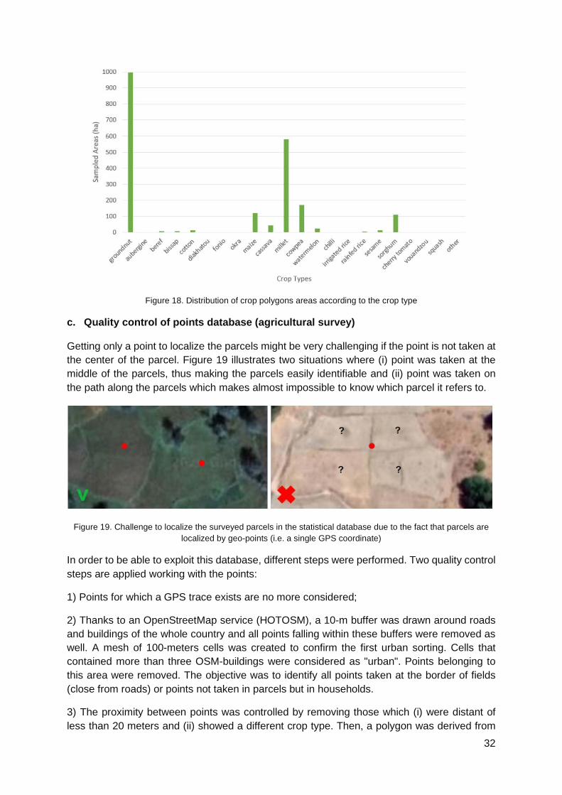
A last criterion was applied for the polygon to be included in the calibration database: their minimum area should cover at least 8 pixels, which removed another 210 polygons. At the end, the database counted 1,593 features, representing 2089 ha shared unequally into 22 crop type classes (Figure 18).

These parcels boundaries were very useful when building the training dataset of the classification algorithm to complement the information from the points database. Indeed, even if the database includes much more parcels (16,861), these parcels are localized only by a geo point (i.e. a single point with GPS coordinates), which can create confusion depending on the exact location of the points (see next section) and which in any case, will cover a much smaller area (1 point = 1 pixel).

32

Figure 18. Distribution of crop polygons areas according to the crop type

c. Quality control of points database (agricultural survey)

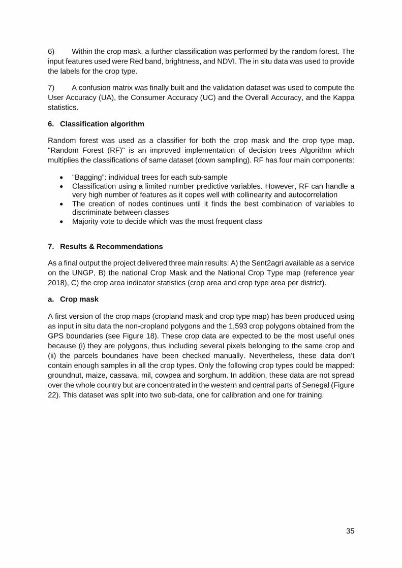
Getting only a point to localize the parcels might be very challenging if the point is not taken at the center of the parcel. Figure 19 illustrates two situations where (i) point was taken at the middle of the parcels, thus making the parcels easily identifiable and (ii) point was taken on the path along the parcels which makes almost impossible to know which parcel it refers to.

Figure 19. Challenge to localize the surveyed parcels in the statistical database due to the fact that parcels are localized by geo-points (i.e. a single GPS coordinate)

In order to be able to exploit this database, different steps were performed. Two quality control steps are applied working with the points:

1) Points for which a GPS trace exists are no more considered;

2) Thanks to an OpenStreetMap service (HOTOSM), a 10-m buffer was drawn around roads and buildings of the whole country and all points falling within these buffers were removed as well. A mesh of 100-meters cells was created to confirm the first urban sorting. Cells that contained more than three OSM-buildings were considered as "urban". Points belonging to this area were removed. The objective was to identify all points taken at the border of fields (close from roads) or points not taken in parcels but in households.

3) The proximity between points was controlled by removing those which (i) were distant of less than 20 meters and (ii) showed a different crop type. Then, a polygon was derived from

33

each remaining geo-point by applying a 20-m buffer. Working with these polygons, the following steps were conducted:

• The 20-m circles which overlapped GPS polygons were removed. At this stage, it remained 12,056 crop points;

• The homogeneity of the 20-m circles was checked. It was assumed that if the point was taken in the middle of the parcel, the resulting polygon would be homogeneous. Conversely, a point taken along the parcel would result in a heterogeneous polygon (mixing different parcels or crop types or including other land cover types such as roads or trees). The homogeneity of each polygon thus checked by looking at the NDVI standard deviation within the polygon along the growing season. Buffers that showed a high standard deviation on their surface were considered as too heterogeneous and were removed. Buffers that had a medium standard deviation were kept but shrunk to a 5m-radius buffer.

• We observed that geo-points corresponding to “rice” were mostly located at the edges of the fields and thus included in heterogeneous 20-m circles and removed. In order to keep a good representation of rice in the reference database, all geo-points were replaced manually in the middle of the fields thanks to Google Earth imagery.

d. Creation of non-cropland reference dataset

Since the agricultural census only focused on agricultural parcels and on surveying crop types, non-crop information has been collected by visual interpretation of very high spatial resolution Google Earth and Planet imagery (Figure 20). In total, 3,004 non-crop polygons were manually drawn across the country, representing 22,188 ha divided into 14 land cover classes (Figure 21).

Figure 20. Interpretation of non-cropland information by visual interpretation of very high resolution imagery: Build up, water body, close forest

34

Figure 21. Distribution of non-crop polygons superficies according to land cover

5. Proposed or implemented methodology.

The project was implemented using the Sen2Agri tool box developed by ESA with contribution from FAO, and deployed on the UN Global platform. Sen2-Agri processors are based on the algorithm of Random Forest.

The main steps of the methodology were:

1) Acquisition of in situ data, QA-QC and enhancement, and split into training (70%) and validation (30%) subset

2) Production of analysis ready data (ARD) from the L2A Sentinel, this in strict connection to the data requirements of the Random Forest Classifier. In fact, such classifier uses the dates of reflectances / vegetation indices, and therefore it is important to have the same dates throughout the area regardless of acquisition orbits of the Sentinel-2. In this context the L2A time series was subjected to “gap filling” to interpolate missing values due to clouds and was temporally resampled to finally produce a time series of 10 days’ composites for the entire agricultural season time window.

3) Features were extracted at each in situ location from the L2A gap filled time series (Red band, NIR band, brightness, NDVI, LAI)

4) An priori stratification of the national territory into smaller ""homogeneous"" regions was carried out based on agro-ecological zones, with the scope of improving the accuracy of the classification work with two main impacts:

• No need for a complete learning set for each tile: the model is taught by stratum • Allowing to manage agro-climatic gradients, with different classification models

5) A random forest classifier was used to generate a crop mask. The NDVI features were used as inputs and the in situ data as labels for crop and non-crop.

35

6) Within the crop mask, a further classification was performed by the random forest. The input features used were Red band, brightness, and NDVI. The in situ data was used to provide the labels for the crop type.

7) A confusion matrix was finally built and the validation dataset was used to compute the User Accuracy (UA), the Consumer Accuracy (UC) and the Overall Accuracy, and the Kappa statistics.

6. Classification algorithm

Random forest was used as a classifier for both the crop mask and the crop type map. "Random Forest (RF)" is an improved implementation of decision trees Algorithm which multiplies the classifications of same dataset (down sampling). RF has four main components:

• “Bagging”: individual trees for each sub-sample • Classification using a limited number predictive variables. However, RF can handle a

very high number of features as it copes well with collinearity and autocorrelation • The creation of nodes continues until it finds the best combination of variables to

discriminate between classes • Majority vote to decide which was the most frequent class

7. Results & Recommendations

As a final output the project delivered three main results: A) the Sent2agri available as a service on the UNGP, B) the national Crop Mask and the National Crop Type map (reference year 2018), C) the crop area indicator statistics (crop area and crop type area per district).

a. Crop mask

A first version of the crop maps (cropland mask and crop type map) has been produced using as input in situ data the non-cropland polygons and the 1,593 crop polygons obtained from the GPS boundaries (see Figure 18). These crop data are expected to be the most useful ones because (i) they are polygons, thus including several pixels belonging to the same crop and (ii) the parcels boundaries have been checked manually. Nevertheless, these data don’t contain enough samples in all the crop types. Only the following crop types could be mapped: groundnut, maize, cassava, mil, cowpea and sorghum. In addition, these data are not spread over the whole country but are concentrated in the western and central parts of Senegal (Figure 22). This dataset was split into two sub-data, one for calibration and one for training.

36

Figure 22. Location of the 1,593 crop polygons obtained from the GPS boundaries

Figure 23 and Figure 24 present the national 10-m spatial resolution cropland mask obtained at the end of the season.

Figure 23. Overview of the cropland mask (V1.0) at national scale

(black = non cropland, white = cropland)

37

38

Figure 24. Zooms of the cropland mask (V1.0) in the right column (black = non cropland) overlaid with Google Earth imagery (left column)

The overall accuracy of the crop mask is 96% and the F-Score values for the cropland and non-cropland classes are of 97% and of 88%, respectively. A visual inspection of the map reveals that it performs relatively well: the discrimination is well done between cropland and the natural shrub and tree vegetation, the urban areas and the bare soil (Figure 24a, b and d). The discrimination with the grassland is however of lower quality (Figure 24 c). It shall also be noted that the irrigated perimeters are not well identified as cropland (Figure 24 e), which is in fact quite logical because this crop class is poorly represented in the in situ data (Figure 18). A post-classification filtering could also be applied to remove the salt-and-pepper effect.

b. Crop type map

Figure 25 and Figure 26 present the national 10-m spatial resolution crop type map obtained at the end of the season, with the national cropland mask on top.

A visual analysis of the crop type map shows that the patterns of the fields are generally well identified. Yet, it can note that there was a strong contamination of groundnut (arachide) and cassava (manioc). Interestingly, the irrigated fields which were not correctly identified in the cropland mask are correctly delineated in the crop type map, but of course they are not

39

associated with the correct label. This only proves that the Sentinel-2 10-m spatial resolution images have the capacity of mapping crop types at the field-level.

Figure 25. Overview of the crop type map (V1.0) at national scale

(non cropland areas from the cropland mask being mapped in white)

Figure 26. Zooms of the crop type map (V1.0) overlaid with Google Earth imagery

The confusion matrix of the crop type map is shown in Table 5, focusing only on the crops that were significantly represented in the in situ data set (Figure 18). The overall accuracy is of 68%

40

and the matrix reflects the significant contamination of the groundnut and to a lesser extent of the cowpea.

Table 5. Confusion matrix of the Crop Type map (V1.0)

c. Crop maps V2.0 (based on GPS traces and points database)

A version 2.0 of the crop type map has been produced integrating also the points database in the training dataset. Even if the reliability of the GPS traces is higher, the points are needed to improve the representativeness of the different crop types in the in-situ calibration dataset, and thus the overall classification performance. Buffered points database and GPS polygons data base were merged. When looking at the sample distributions between crop types, it was visible that groundnut was over-represented, as well as rice but to a lesser extent.

After several tries, it was decided to limit the number of samples for these two crops: the area of the groundnut samples could not exceed 400 ha while for the rice, the threshold was set to 100 ha. The final samples distribution is illustrated in Figure 27, in which the mentioned thresholds are visible (rice class covering both rainfed and irrigated rice). Their spatial distribution is shown in Figure 28. In total, for the version 2, the Sen2-Agri system was launched with a reference dataset including 4,252 crop features (1,086 ha) and 3,000 non-crop features (18,039ha)

41

Figure 27. Distribution of non-crop polygons superficies according to land cover (V2.0)

Figure 28. Localization of the 4,252 crop polygons and buffered points obtained from the GPS data base

Figure 29 presents the 2nd version of the national 10-m spatial resolution crop type map obtained at the end of the season, with the national cropland mask on top.

42

Figure 29. Overview of the crop type map (V2.0) at national scale

(non-cropland areas from the cropland mask being mapped in white)

The confusion matrix of the crop type map is shown in Table 6, focusing only on the crops that were significantly represented in the in situ data set. The overall accuracy is 78% and the matrix reflects the slight contamination between maize, sorghum and millet. The groundnut contamination seems to be very lower than in the 1st version and cowpea and sorghum are better recognized.

Table 6. Confusion matrix of the Crop Type map (V2.0)

43

d. Crop area indicators

Next to the crop maps, a second type of products generated was the crop area indicators. The aim of this crop area indicators is not to replace or to be equivalent to the agricultural statistics. It is derived from EO data and is in any case less accurate. Yet, the indicators have the advantage of being directly derived from the crop maps, and thus of being available much before the statistics (which usually come 6 months after harvest). The interpretation of these figures needs to be done having in mind the accuracy assessment of the crop maps (quantitative figures and visual assessment). Based on the cropland mask, the following crop / no crop indicators can be derived at national and provincial levels (

44

Table 7).

As just mentioned, these figures need to be taken cautiously, given the general under-estimation of the cropland in the product. The same kind of indicators can be derived from the crop type map, focusing on the main crops that are possible to discriminate given the available in situ datasets, i.e. groundnut, maize, millet, cowpea, sorghum.

Results are based on the 2nd version of the crop type map, which is much better. The accuracy assessment of the crop type map has shown a good accuracy for all the crops, but still with an overestimation of groundnut and millet. This conclusion is confirmed - especially for the millet - when comparing the area indicators with the FAO Statistics: the explanation comes probably from the fact that the cropland mask (which overlays the crop type map) is still impacted by significant errors. Yet, the area indicators of the other crops seem to be really closed to the FAO Statistics which are taken as reference.

45

Table 7. Cropland - non cropland area indicators at national and provincial level

The same kind of indicators can be derived from the crop type map, focusing on the main crops that are possible to discriminate given the available in situ datasets, i.e. groundnut, maize, millet, cowpea, sorghum (Table 8). These results are based on the 2nd version of the crop type map, which is much better.

Table 8. Area indicators of the main crop types at national scale (V2.0)

The accuracy assessment of the crop type map has shown a good accuracy for all the crops, but still with an overestimation of groundnut and millet. Such over estimation is due to the contamination of those two dominant crop classes into other crop classes as shown in the confusion matrix in Table 6. This conclusion is confirmed - especially for the millet - when comparing the area indicators with the FAO Statistics (Figure 30): the explanation comes probably from the fact that the cropland mask (which overlays the crop type map) is still impacted by significant errors. Yet, the area indicators of the other crops seem to be really closed to the FAOSTAT which were taken as reference.

46

Figure 30. Comparison of the main crop types area obtained from EO data (blue) and as reported in the FAOSTAT (orange) (V2.0)

It should be reminded that the ultimate quality of a crop type map, hence its accuracy, heavily depends on the quality of the in-situ data that is used to train the algorithm and to validate its result. A high quality in-situ data set should provide information of crop locations across all agroecological zones in the effort to reflect as much as possible the variability of conditions. In which crops are grown. The proper positioning of the GPS in the field is another element of quality, jointly with the accuracy of the instrument.

In order to improve the quality of EO products, FAO is supporting countries in the optimization of survey design, using geospatial datasets for stratification and probabilistic sampling.

8. Solution Architecture

Software used for the EO preprocessing and analysis was the Sen2Agri tool box. The requirements for such tool box were assessed as:

• number of tiles: 40 Sentinel-2; • on average (accounting for cloud cover), we can assume having 6 valid products by

month (valid meaning less than 90% cloud cover); • it results in a total of 2,880 Level 2A products to be processed (40*6*12); • assuming that the size of one L2A product is around 1.6GB, we need minimum around

4,600 GB for the storage. Six TB would be more comfortable; • SSD storage is considered as optional but has been required to install the system

(minimum of 50 GB).

47

Infrastructure: FAO partnered with the UN Big Data Working Group who provided technical assistance to deploy the Sen2Agri tool box on the UNGP

The platform has been set up by the UN Group. The technical working group (University of Louvain) had access to the required infrastructure which was equipped with the relevant software. The main assets of the UN Global Platform are:

• to provide storage and computing power; • to provide an optimized for performance and low running costs; • to be scalable; • to secure hosting of country data; • to allow the sharing of trusted data, methods and algorithms; • to be potentially an incubator/accelerator for innovations; • to facilitate the dissemination/visibility; • to ensure an easy deployment of Sen2-Agri tool box.

The infrastructure was implemented so that the installation script could be easily replicated. This to make the uptake easier and second, to facilitate the deployment of the tool during the activity. The solution diagram as implemented by the UN Global Platform is presented in Figure 31.

Figure 31. UN Global Platform solution diagram for the EO-STAT project in Senegal

In June 2020, a group of EO experts in Senegal was created and they were presented with the platform and the tool through a first training. The composition of this expert group will evolve for the last months of the project, with new partners coming also from ANSD, ISRA and CSE

9. Terminology

Random forest, Temporal composites, Sen2Agri toolbox

48

10. Bibliography

Matton N. et al., An Automated Method for Annual Cropland Mapping along the Season for Various Globally-Distributed Agrosystems Using High Spatial and Temporal Resolution Time Series, Remote Sens. 2015, 7, 13208-13232

Valero S. et al., Production of a Dynamic Cropland Mask by Processing Remote Sensing Image Series at High Temporal and Spatial Resolutions. Remote Sens. 2016, 8, 55.

49

Improvement of land cover classification process using Machine Learning in cloud computing from Sentinel-2 satellite images with RPAS image injection. Submitted by: National Administrative Department of Statistics (DANE)3

1. Project background

The project started in 2019 as part of the work done by the Geostatistical Development and Research Unit of the Geostatistics Directorate of the Colombian National Statistical Office (DANE for its acronym in Spanish).

To obtain accurate information on land cover changes in the agricultural sector over Colombia, DANE has proposed a supervised classification method that integrates Sentinel-2 satellite imagery with images collected from Remotely-piloted Aircraft System (RPAS) for the improvement and continuous updating of the land cover variable of the Rural and Agricultural Master Framework. This method uses Earth Observation (EO) data and applies techniques to strengthen the production of agricultural statistical information in Colombia by offering more reliable data for the design of the National Agricultural Survey4.

This project enabled the Geostatistics Directorate to apply alternative methods for obtaining information with greater precision on the land cover and contributing to the generation of statistical information on the Colombian agricultural sector.

2. Study areas

The study was carried out in four municipalities of Colombia (see Figure 32) where there was available RPAS images: Salento (Quindio), Tununguá, Pajarito and Cómbita in the department of Boyacá.

3 The source of this case study is: Ramírez, M., Martínez, L., Montilla, M., Sarmiento, O., Lasso, J., & Díaz, S. (2020). “Obtaining agricultural land cover in Sentinel-2 satellite images with drone image injection using Random Forest in Google Earth Engine”. Revista de Teledetección, 0(56), 49-68. doi: https://doi.org/10.4995/raet.2020.14102 4 “This Survey seeks to estimate the use of land, size and distribution of sampling segments. It also provides data on the area, production and yield of major temporary and permanent crops; pasture area, milk production, and livestock inventory”. https://www.dane.gov.co/index.php/en/statistics-by-topic-1/agricultural-sector/national-agricultural-survey-ena

50

Figure 32. Location of study areas for DANE’s project.

Source: Adapted from Ramírez, M., Martínez, L., Montilla, M., Sarmiento, O., Lasso, J., & Díaz, S. (2020).

3. EO data / preprocessing

Sentinel-2, the multispectral high-resolution imaging mission enabled users to access images in the repository of the Google Earth Engine (GEE) at 2A processing level. These images were used for their spectral bands of spatial resolution of 10 or 20 meters.

To ensure the land use coherence obtained from both sources, Sentinel-2 and RPAS images, the existence of a temporal correspondence was required, so the selected collection date of the satellite image in each one of the study areas were similar to the one of the RPAS images. In Table 9, the Sentinel-2 images collection date range used is showed, as well as, the number of images required. Due to COVID-19 mobility restrictions, RPAS datasets captured by other public entities were used as input to classify crops in different spatial and temporal frameworks to those initially proposed.

Table 9. Characteristics of the Sentinel-2 images collection.

Study area Date Range Number of images Salento 11/09/2019 2 Tununguá 07/08/2018 1 Pajarito 24/08/2018 to 18/09/2018 3 Cómbita 01/01/2019 1 Source: Adapted from Ramírez, M., Martínez, L., Montilla, M., Sarmiento, O., Lasso, J., & Díaz, S. (2020).

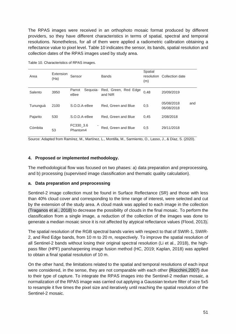
51

The RPAS images were received in an orthophoto mosaic format produced by different providers, so they have different characteristics in terms of spatial, spectral and temporal resolutions. Nonetheless, for all of them were applied a radiometric calibration obtaining a reflectance value to pixel level. Table 10 indicates the sensor, its bands, spatial resolution and collection dates of the RPAS images used by study area.

Table 10. Characteristics of RPAS images.

Area Extension (Ha) Sensor Bands

Spatial resolution (m)

Collection date

Salento 3950 Parrot Sequoia-eBee

Red, Green, Red Edge and NIR 0,48 20/09/2019

Tununguá 2100 S.O.D.A-eBee Red, Green and Blue 0,5 05/08/2018 and 06/08/2018

Pajarito 530 S.O.D.A-eBee Red, Green and Blue 0,45 2/08/2018

Cómbita 53 FC330_3.6 -Phantom4 Red, Green and Blue 0,5 29/11/2018

Source: Adapted from Ramírez, M., Martínez, L., Montilla, M., Sarmiento, O., Lasso, J., & Díaz, S. (2020).

4. Proposed or implemented methodology.

The methodological flow was focused on two phases: a) data preparation and preprocessing, and b) processing (supervised image classification and thematic quality calculation).

a. Data preparation and preprocessing

Sentinel-2 image collection must be found in Surface Reflectance (SR) and those with less than 40% cloud cover and corresponding to the time range of interest, were selected and cut by the extension of the study area. A cloud mask was applied to each image in the collection (Traganos et al., 2018) to decrease the possibility of clouds in the final mosaic. To perform the classification from a single image, a reduction of the collection of the images was done to generate a median mosaic since it is not affected by atypical reflectance values (Flood, 2013).

The spatial resolution of the RGB spectral bands varies with respect to that of SWIR-1, SWIR-2, and Red Edge bands, from 10 m to 20 m, respectively. To improve the spatial resolution of all Sentinel-2 bands without losing their original spectral resolution (Li et al., 2018), the high-pass filter (HPF) pansharpening image fusion method (HC, 2019; Kaplan, 2018) was applied to obtain a final spatial resolution of 10 m.

On the other hand, the limitations related to the spatial and temporal resolutions of each input were considered, in the sense, they are not comparable with each other (Rocchini,2007) due to their type of capture. To integrate the RPAS images into the Sentinel-2 median mosaic, a normalization of the RPAS image was carried out applying a Gaussian texture filter of size 5x5 to resample it five times the pixel size and iteratively until reaching the spatial resolution of the Sentinel-2 mosaic.

52

Once the images had the same spatial resolution, the bands from the Sentinel-2 median mosaic and the resampled RPAS bands were stacked into one raster file. Additionally, to improve the differentiation of the coverages of interest, the subset of the 30 m spatial resolution DEM SRTM available in the GEE repository and its slope raster, calculated from the DEM, were added to the stacked raster.

b. Processing

To improve the final classification, the most used spectral indices for agricultural applications were calculated using the median mosaic and the resampled RPAS bands.

The supervised classification was performed to the Sentinel-2 image including the RPAS image and in order to be able to make a comparison it was also done using exclusively Sentinel-2 images. Initially, a thematic expert manually digitalized the set of crop seeds, using the categorization of coverages established by the Colombian Rural and Agricultural Master Framework. The sample dataset was divided into two groups, the first one corresponding to the training data and the other one, to be used with validation purposes. For the selection of the validation data set, the recommendations made by Millard and Richardson (2015) were taken, in which 30% of the total sample corresponds to it and without spatial autocorrelation with the training sample.

As indicators of the thematic quality of the overall classification were used the most representative metrics that correspond to percentage of map classification and kappa index that does not have bias derived from the errors of omission and commission (Foody, 2002; Liu et al., 2007). At the coverage level, errors of omission and commission were calculated. Those indices were derived from the confusion matrix generated from the comparison of the classification result with the validation data.

5. Classification algorithm

The supervised classification was performed using the Random Forest learning method, which is the most common and with the best thematic accuracy for agricultural information production (Belgiu & Drăgu, 2016; Chen et al., 2017; Dash et al., 2018; Zhao et al., 2019)). The parameters used were 100 trees and 4 branches; the number of branches was established according to the theoretical recommendation of Belgiu & Drăgu, (2016) who argue that it should be the square root of the number of target classes.

6. Results & Recommendations

As it was mentioned in the methodology, to perform the injection of the RPAS images to the Sentinel-2 mosaic, it was necessary to make an iterative resampling process by applying a Gaussian filter. Figure 33 shows the result of the resampling process in an area with multiple coverages. From the visual analysis it was evident that the resampled image retained the texture characteristics of the original one, despite the spatial generalization. Consequently, the resampled image enriches the coverage classification process.

53

Figure 33. Visual comparison among images.

Source: Adapted from Ramírez, M., Martínez, L., Montilla, M., Sarmiento, O., Lasso, J., & Díaz, S. (2020).

Analyzing visually the result of the classifications, despite not finding significant improvements in the classification that included RPAS images compared to the one made with Sentinel-2 images only, in specific cases, improvements were evident in the definition of coverage limits. As an example Figure 34 rows A and C, there was a better delimitation for the forest cover and in row B, a better delimitation of the river was observed.

Figure 34. Classification visual comparison.

Source: Translated from Ramírez, M., Martínez, L., Montilla, M., Sarmiento, O., Lasso, J., & Díaz, S. (2020).

Nevertheless, the general accuracy and the Kappa index were increased when the classification was performed using the integration of the Sentinel-2 image with the RPAS image, fluctuating from 1.1% to 26.7% (see Table 11), which allows to affirm that the injection of the RPAS image to Sentinel-2 images improves the cover land classification results.

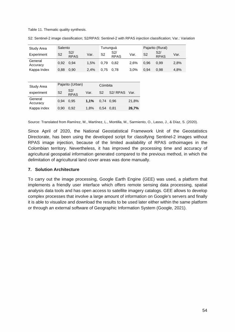
54

Table 11. Thematic quality synthesis.

S2: Sentinel-2 image classification; S2/RPAS: Sentinel-2 with RPAS injection classification; Var.: Variation

Study Area Salento Tununguá Pajarito (Rural)

Experiment S2 S2/ RPAS Var. S2 S2/

RPAS Var. S2 S2/ RPAS Var.

General Accuracy 0,92 0,94 1,5% 0,79 0,82 2,6% 0,96 0,99 2,8%

Kappa Index 0,88 0,90 2,4% 0,75 0,78 3,0% 0,94 0,98 4,8%

Study Area Pajarito (Urban) Cómbita

experiment S2 S2/ RPAS Var. S2 S2/ RPAS Var.

General Accuracy 0,94 0,95 1,1% 0,74 0,96 21,8%

Kappa index 0,90 0,92 1,8% 0,54 0,81 26,7%

Source: Translated from Ramírez, M., Martínez, L., Montilla, M., Sarmiento, O., Lasso, J., & Díaz, S. (2020).

Since April of 2020, the National Geostatistical Framework Unit of the Geostatistics Directorate, has been using the developed script for classifying Sentinel-2 images without RPAS image injection, because of the limited availability of RPAS orthoimages in the Colombian territory. Nevertheless, it has improved the processing time and accuracy of agricultural geospatial information generated compared to the previous method, in which the delimitation of agricultural land cover areas was done manually.

7. Solution Architecture

To carry out the image processing, Google Earth Engine (GEE) was used, a platform that implements a friendly user interface which offers remote sensing data processing, spatial analysis data tools and has open access to satellite imagery catalogs. GEE allows to develop complex processes that involve a large amount of information on Google's servers and finally it is able to visualize and download the results to be used later either within the same platform or through an external software of Geographic Information System (Google, 2021).

55

8. Bibliography

Belgiu, M., & Drăgu, L. (2016). Random forest in remote sensing: A review of applications and future directions. In ISPRS Journal of Photogrammetry and Remote Sensing (Vol. 114, pp. 24–31). Elsevier B.V. https://doi.org/10.1016/j.isprsjprs.2016.01.011 Chen, W., Xie, X., Wang, J., Pradhan, B., Hong, H., Bui, D. T., Duan, Z., & Ma, J. (2017). A comparative study of logistic model tree, random forest, and classification and regression tree models for spatial prediction of landslide susceptibility. Catena, 151, 147–160. https://doi.org/10.1016/j.catena.2016.11.032 Dash, J. P., Pearse, G. D., & Watt, M. S. (2018). remote sensing UAV Multispectral Imagery Can Complement Satellite Data for Monitoring Forest Health. https://doi.org/10.3390/rs10081216 FAO (2011) https://www.google.com/url?sa=t&rct=j&q=&esrc=s&source=web&cd=&ved=2ahUKEwj5poGDhffxAhVdQzABHZOdAFIQFjACegQICBAD&url=http%3A%2F%2Fwww.fao.org%2Ffileadmin%2Ftemplates%2Fess%2Fess_test_folder%2Fdocuments%2FProduction_trade%2Fdefinitions%2FCrops_statistics_concepts_definitions_classifications.doc&usg=AOvVaw0B90MwHjlpPbWQ_Lt27tXz Flood, N. (2013). Seasonal Composite Landsat TM/ETM+ Images Using the Medoid (a Multi-Dimensional Median). Remote Sensing, 5(12), 6481–6500. https://doi.org/10.3390/rs5126481 Foody, G. M. (2002). Status of land cover classification accuracy assessment. Remote Sensing of Environment, 80(1), 185–201. https://doi.org/10.1016/S0034-4257(01)00295-4 Google. (2021). Google Earth Engine: A planetary-scale platform for Earth science data & analysis. https://earthengine.google.com/ HC, T. (2019, July). Pansharpening Sentinel-2 imagery in Google Earth Engine. Ingeoexpert. (2020). Clasificaciones de imágenes de satélite. https://ingeoexpert.com/articulo/clasificaciones-de-imagenes-de-satelite/ Kaplan, G. (2018). Sentinel-2 Pan Sharpening—Comparative Analysis. Proceedings, 2(7), 345. https://doi.org/10.3390/ecrs-2-05158 Li, Y., Qu, J., Dong, W., & Zheng, Y. (2018). Hyperspectral pansharpening via improved PCA approach and optimal weighted fusion strategy. Neurocomputing, 315, 371–380. https://doi.org/10.1016/j.neucom.2018.07.030 Liu, C., Frazier, P., & Kumar, L. (2007). Comparative assessment of the measures of thematic classification accuracy. Remote Sensing of Environment, 107(4), 606–616. https://doi.org/10.1016/j.rse.2006.10.010 Millard, K., & Richardson, M. (2015). On the Importance of Training Data Sample Selection in Random Forest Image Classification: A Case Study in Peatland Ecosystem Mapping. Remote Sensing, 7(7), 8489–8515. https://doi.org/10.3390/rs70708489 Rocchini, D., 2007. Effects of spatial and spectral resolution in estimating ecosystem α-diversity by satellite imagery. Remote Sensing of Environment, 111(4), 423–434.

56

Traganos, D., Aggarwal, B., Poursanidis, D., Topouzelis, K., Chrysoulakis, N., Reinartz, P., 2018. Towards global-scale seagrass mapping and monitoring using Sentinel-2 on Google Earth Engine: The case study of the Aegean and Ionian seas. Remote Sensing, 10(8), 1227. Zhao, L., Shi, Y., Liu, B., Hovis, C., Duan, Y., & Shi, Z. (2019). Finer Classification of Crops by Fusing UAV Images and Sentinel-2A Data. Remote Sensing, 11(24), 3012. https://doi.org/10.3390/rs11243012

57

Earth Observation data analytics for Greenhouse detection and production area estimation Submitted by: Statistics Canada 1. Project background Statistics Canada’s greenhouse project has been using satellite imagery for identification of greenhouses within major greenhouse growth areas in Southern Ontario since 2014. In 2018, the proposal to expand and automate the identification process was accepted and navigated towards a machine learning approach. The new approach to the identification of greenhouses, using new technologies, was responding to call at Statistics Canada to integrate more administrative data sources, such as satellite imagery, to replace survey questions or reduce the need for survey respondents, in addition to applying a timelier approach to producing estimates. The Agriculture Division created the Ag-Zero project, which is aimed to replace conventional surveys with alternative data sources and data collection methods in replacement of some fundamental questionnaires.

The first iteration of the use of satellite imagery for the identification of greenhouses was performed in 2018-2019 where five-meter resolution Rapid Eye imagery was used. This imagery included five bands, three of which were for vegetation analysis. The project study area was within three substantial greenhouses economic regions within Canada: Fraser Valley, British Columbia, Essex County, Ontario and Niagara County, Ontario. The satellite data was accompanied by hand-digitized greenhouse GIS data as training and verification.

The project focused on the use of open data sources to identify greenhouses, which allowed the project to be placed onto the new Azure Microsoft Cloud on boarded with a NVIDIA Tesla V100 GPU 114 GB RAM, 1 TB premium SSD, 10 TB storage account. Access to these online cloud resources had resolved many of our storage and processing questions, which we encountered during the project’s proposal period.

The primarily goal of the second stage of the project in 2019 was to refine the machine learning technique used, but also to provide a more realistic cost saving approach to widespread annual earth observation coverage – which, with the previous use of Rapid Eye imagery, was not obtainable at the time for total agricultural land coverage across Canada. Open source, high resolution aerial imagery was available from provincial and municipal GIS websites for download. Imagery in this form was encountered in 23 municipalities across 5 provinces. This data had 3 or 4 bands and ranged in pixel resolution between 0.30m -0.07m – which provided the resolution needed to detect greenhouses independent of size. In addition, the machine learning technique had migrated from a pixel-by-pixel classifier, convolutional neural network – to an image segmentation and object identification method by means of a U-Net with Res-Net neural network classifier. The analysis for this second round of the project was done on secure offline GPU housed within Statistics Canada.

In addition to the use of aerial imagery, mid-range resolution Sentinel-2 10m imagery was also used for the identification of greenhouses which had evidence of vegetation inside for Spring 2019. This development for classifying greenhouses is deemed important for understanding production cycles of greenhouses while utilizing open source imagery availability for a routine update, as the satellite imagery’s revisit time is approximately every 5-10-days. The results of the second phase development for the greenhouse identification project using high resolution aerial imagery were improved from the first phase.

2. Study areas

58

Niagara, Ontario

Essex, Ontario

3. EO data / preprocessing Greenhouse Detection: Aerial imagery, spatial Resolution 0.1-0.3m, bands used: Red, Green, Blue, Near-infrared, indices: Normalized Difference Vegetation Index (NDVI)

Greenhouse Area Production Monitoring: Sentinel-2 imagery, spatial resolution: 10m, bands used: red, green, blue, near-infrared, indices: NDVI

4. In situ data Hand digitized greenhouse polygons in the area of interest. Number of shapes: 620 representing 2,710,439 square meters of greenhouse area.

5. Proposed or implemented methodology. a. Area of interest

Part of the work for the Phase 2 project, was ensuring that there was a significant coverage by aerial imagery of agricultural area in Canada. Other elements of the imagery include: how it can be obtained, metadata and how often it was collected. It was found that there were many provincial and municipal resources available, in high quality through provincial and municipality open source websites. Imagery was available, in BC, Alberta, Manitoba, Ontario, and New Brunswick. Further, data partnerships were established with Niagara and Brampton, Ontario – where interest in the greenhouse project helped obtain in house data through data acquisition agreements, free of cost. During the course of the project, January 2020 to March 2020, two areas of interest were used for machine learning training and testing: Niagara County and Essex County in Ontario. All other areas were obtained to get a better understanding of the resources available for when the project is approved for further testing and training.

b. Ground -Truth Data

For the machine learning classification and deep learning methods, ground-truth data in the form of geographic shapefiles were necessary for both the training and testing sites. The ground truth data provide a view of what in the imagery would be considered a greenhouse, and what was not, this provided in binary values within the provided imagery. The data from training sites are used to train the machine learning model while the testing sites are used to calculate the precision and accuracy of the trained model. The training sites also provide information of the spectral details of the greenhouses for training the algorithm, so that when testing and production efforts are in effect, the algorithm can find greenhouses within imagery, with little to no error, based on previously obtained details of what to search for. These are therefore some of the most important steps taken, and some of the most effort in the project as a result. In an ideal production scenario, aerial imagery from across the country would be provided to the algorithm trained on detecting greenhouses as the geography and surrounding terrain varies significantly

For the estimation of greenhouse production area, the ground-truth data served another purpose in reducing the areas of attribute extraction from the vegetation analysis raster layer, to gain area estimation within the greenhouses.

c. Aerial Imagery

59

The imagery from Niagara, Ontario was from spring 2018 at 0.16m pixel resolution, presented in 1km x 1km tiles. The acquisition was collected in the spring of 2018 for a “leaf off” and relatively cloud free image, thus allowing little obstructions in the overall analysis of the underlying buildings. The aerial imagery collection in Niagara, Ontario totaled about 2 TB of data, for this reason only a fraction of the data was used for analysis to those tiled areas which contain known greenhouses, as the entire set presented storage and data processing issues.

d. Satellite imagery

The area of interest for the satellite imagery was concentrated in the three areas of the highest number of greenhouses in Canada: Niagara, Fraser and Essex County. Since the greenhouses should already be detected by this stage, it should not be necessary to have less than 10 meter resolution for the imagery to use in practice.

For the estimation of the production area of the greenhouses, it has been proven necessary to look for another means of imagery which is still open source, and provides equal coverage across the country. For this reason, Sentinel-2 imagery with 4 bands (red, green, and blue, near infrared) at 10 meter pixel resolution was chosen. It is used for estimating the total area within the greenhouse for production. There is no limitation, minus the appearance of clouds, which reduces visibility and natural vegetation. The repeat schedule for the acquisition was approximately every 5 to 10 days for coverage across the globe. This also allowed a more seasonal estimation of the greenhouses production estimations as they change throughout the season.

e. Machine learning classification and Deep Learning methods

The machine learning project utilized the higher resolution aerial imagery discussed above (with pixel resolution between 0.075 meters and 0.20 meters and 3 or 4 spectral bands).

The machine learning consists of two components:

• Training, during which the machine learning algorithm was fed images from “training sites” together with the labels (identifiers specifying exactly which pixels in the image correspond to greenhouses) and had to determine which patterns in the images corresponded to greenhouses. A machine learning model that can be applied to new images was the output of this phase.

• Testing, in which the model was applied to “testing sites” that were disjoint from the training sites. The model generated predictions for every pixel in the testing sites, which were then compared to the ground truth. From this model quality estimates were produced.

For this project, Statistics Canada used U-Net based convolutional neural network architectures for image segmentation. The U-Net architecture generated predictions for each pixel in the image, effectively highlighting areas of interest.

60

f. Greenhouse production

In order to provide an accurate representation of the greenhouse industry in Canada, it was therefore necessary to not only find the total greenhouse area, but the total greenhouse production area, as this is the concept surveyed in the census of agriculture. The greenhouse production area model also provided an understanding of the consistencies within the greenhouse sector, along with the successes of the greenhouse and agriculture industry. As a response, a remote sensing approach was used to monitor the greenhouse production inside the greenhouses. Using vegetation indices and analysis of the greenhouse shapes, allowed the area of greenhouses within the buildings to be monitored. Further, the analysis was done multiple times within a year, with Sentinel-2 multispectral data, which is free and open data. This analysis was completed on Essex County, Ontario with success in 2018 and 2019 datasets.

6. Classification algorithm Machine Learning

• Batch size: 64 • Loss function: dice loss • Optimizer: RMSprop • Learning rate: 10-5 • Weight decay (L2 regularization): 10-6

7. Results & Recommendations

a. Greenhouse Detection model

The classifier for Greenhouse detection in aerial images did very well for the vast majority of areas. In eleven areas the MCC (Matthews Correlation Coefficient) is between 0.9 and 1.0, in five areas the MCC is between 0.8 and 0.9, and in three areas the MCC is less than 0.8. In all areas with a large number of greenhouses, the MCC is at least 0.8 and is usually over 0.9.

Further testing on ResNet and DenseNet architectures are planned for future phases of the greenhouse detection project to improve testing accuracy. A future phase will be to explore other greenhouse classifications from the high-resolution imagery, such as the cover type.

b. Greenhouse Production model Although there was insufficient data to validate the model at the time, the classification of the greenhouses under production performed well given the understanding of the greenhouse industry and the science behind the use of an NDVI for vegetation analysis. The next iteration of the project, ongoing in 2021-2022, will be modelled using fine resolution validation data, which will allow the model to move into a production environment.

The model performed well in areas of large greenhouses, such as Essex County in Ontario, but the greenhouses were harder to identify with the NDVI at the 10m level in areas such as Niagara, Ontario and Fraser Valley in British Columbia because of the larger area of interest and the smaller, on average, size of the greenhouses. This has caused the research team to

61

look into finer resolution data within the private sector, at the 5m or 1.5m resolution for these areas of interest.

The model was also meant to perform analysis several times a year, within the growing season of the spring and summer; in addition to outside of the growing season in the fall and winter. This has been proven to be difficult in some areas where clouds, rain and snow reduced the effectiveness of the optical satellites. Consequently, the number of iterations in a year was reduced to 2 or 3 times for the model, instead of 4 or 5 times.

8. Solution Architecture The work was done on an in-house GPU system with the following specifications:

• NVidia Quadro P6000 GPU. • Two Intel CPUs with 14 cores each, for total of 28 physical cores and 56 virtual cores. • 256 GB of RAM. • 1 TB SSD with system installation and two 4 TB HDD for storage. • Ubuntu Linux 18.04 LTS. • Necessary software installed such as R, Python, QGIS, NVidia drivers, and CUDA /

cuDNN. • Standalone system not connected to any network. Data transfers to and from the

machine were done using special hardware encrypted external hard drives.

9. Bibliography https://arxiv.org/pdf/1506.01186.pdf Cyclical Learning Rates for Training Neural Networks Leslie N. Smith U.S. Naval Research Laboratory, Code 5514 4555 Overlook Ave., SW., Washington, D.C. 20375 leslie.smith@nrl.navy.mil https://arxiv.org/pdf/1803.09820.pdf US Naval Research Laboratory Technical Report 5510-026 A DISCIPLINED APPROACH TO NEURAL NETWORK HYPER-PARAMETERS: PART 1 – LEARNING RATE, BATCH SIZE, MOMENTUM, AND WEIGHT DECAY Leslie N. Smith US Naval Research Laboratory Washington, DC, USA leslie.smith@nrl.navy.mil

Hill, S. (Jan 14 2020). Unprecedented greenhouse growth won't slow down in 2020. Windsor Star. https://windsorstar.com/news/local-news/unprecedented-greenhouse-growth-wont-slow-down-in-2020/

Rouse, J. R. (1974). Monitoring vegetation systems in the Great Plains with ERTS. Third Earth Resources Technology Satellite - I symposium. Volume I: Technical Presentations (pp. 309-317). Washington, D.C.: NASA SP-351, NASA.

He K., Zhang X., Ren S. and Sun J., "Deep Residual Learning for Image Recognition," 2016 IEEE Conference on Computer Vision and Pattern Recognition (CVPR), Las Vegas, NV, 2016, pp. 770-778, doi: 10.1109/CVPR.2016.90.

Ronneberger O., Fischer P., and Brox T. 2015. “U-Net: Convolutional Networks for Biomedical Image Segmentation,” Navab N., Hornegger J., Wells W., Frangi A. (eds) Medical Image Computing and Computer-Assisted Intervention – MICCAI 2015. MICCAI 2015. Lecture Notes in Computer Science, vol 9351. Springer, Cham.

Pytorch Pretrained Models: https://pytorch.org/docs/stable/torchvision/models.html

62

G. Huang, Z. Liu, L. Van Der Maaten and K. Q. Weinberger, "Densely Connected Convolutional Networks," 2017 IEEE Conference on Computer Vision and Pattern Recognition (CVPR), Honolulu, HI, 2017, pp. 2261-2269, doi: 10.1109/CVPR.2017.243.

The One Hundred Layers Tiramisu: Fully Convolutional DenseNets for Semantic Segmentation (2017 paper by Simon J.M. D., …) Code Repositories

o https://github.com/lyakaap/Kaggle-Carvana-3rd-Place-Solution o https://tuatini.me/practical-image-segmentation-with-unet/ o https://github.com/EKami/carvana-challenge o https://github.com/milesial/Pytorch-UNet o https://github.com/pytorch/pytorch/blob/master/CITATION

63

Understanding the Requirements for Surveys to Support Satellite-Based Crop Type Mapping: Evidence from Sub-Saharan Africa Submitted by: World Bank5

1. Project Background Satellite-based approaches to mapping agricultural outcomes, such as crop-specific estimates of cultivated areas and yields, require data for training and validating the underlying remote sensing models. The quality and spatial resolution of satellite-based estimates is directly impacted by the data used for model training and validation (Lobell et al., 2019, 2020). Recent earth observation research that has focused on low-income countries has relied largely on two sources of training and validation data: (i) manually-labeled optical imagery (DeFourny et al., 2019; Xiong et al., 2017; Wei et al., 2020), and (ii) ground data collection, including as part of household and farm surveys (Hegarty-Craver et al., 2020; Jin et al., 2017, 2019; Kerner et al., 2020; Lambert et al., 2018; Richard et al., 2017). This paper is related to earth observation applications that rely on georeferenced survey data to meet model training and validation needs. Despite the expanding knowledge base regarding the use of earth observation techniques in low-income countries that are primarily characterized by smallholder farming, research studies have largely remained sub-national in scope and have exhibited heterogeneity in terms of the ground data used to fulfill comparable analytical objectives pursued in different settings. Lack of methodological research to identify the required volume of and approach to ground data collection for training and validating remote sensing models is arguably one of the hurdles against the scale-up of satellite-based estimation of agricultural outcomes across countries and expansive geographies. Identifying ground data requirements for key earth observation applications in low-income countries, including high-resolution crop type mapping and crop yield estimation, would be important not only for assessing the utility of existing georeferenced household survey data for earth observation research but also informing the design of future large-scale household and farm surveys that can provide the required training and validation data for downstream earth observation efforts. Against this background, this case study addresses several operational and inter-related research questions in the context of high-resolution maize area mapping in Malawi and Ethiopia: 1) what is the minimum volume of household survey data that is required to reach an acceptable level of accuracy of a crop classification algorithm? and 2) how does the approach to georeferencing plot locations in household surveys impact the accuracy of the same crop classification algorithm? Furthermore, it has been demonstrated how the algorithmic accuracy is affected based on 1) the type of satellite data used (optical only, radar only or both) - given the considerable differences in the complexity and costs of imagery processing across the various options, and 2) whether plots under specific area thresholds are excluded from the training data - given the potential concerns around the mismatch between the relatively small scale of farming in Malawi and Ethiopia and the Sentinel-2 imagery used in our analysis. To our knowledge, this is the first study that attempts to systematically answer these questions in the context of high-resolution crop area mapping in smallholder farming systems.

5 The case study is an excerpt from Azzari, G., Jain, S., Jeffries, G., Kilic, T., and Murray, S. (2021). “Understanding the Requirements for Surveys to Support Satellite-Based Crop Type Mapping: Evidence from Sub-Saharan Africa.” Remote Sensing, 13(23), 4749, https://doi.org/10.3390/rs13234749. The research has been conducted with support from the 50x2030 Initiative to Close the Agricultural Data Gap, as part of the on-going work program to identify the approach to and volume of georeferenced survey data collection for calibrating and validating remote sensing models for high resolution estimation of crop areas and crop yields in smallholder farming systems.

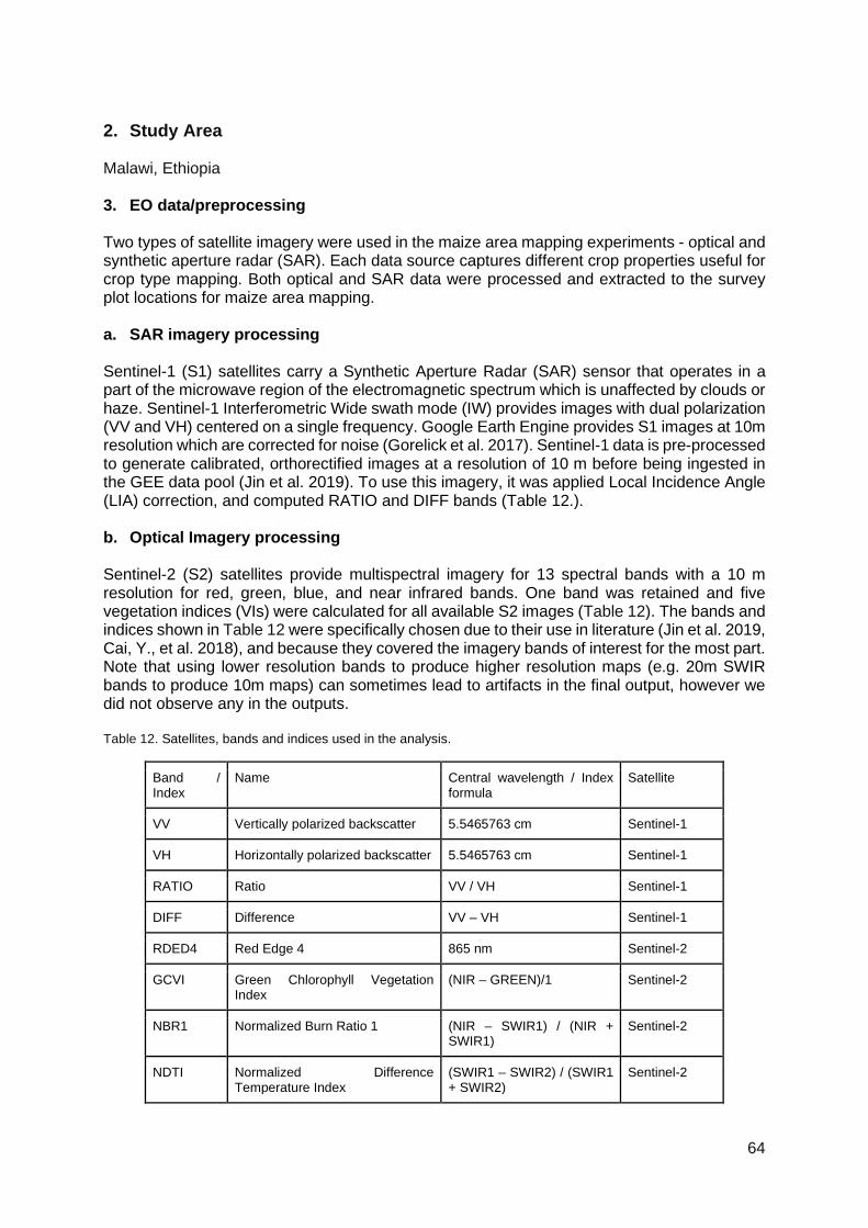
64

2. Study Area Malawi, Ethiopia 3. EO data/preprocessing

Two types of satellite imagery were used in the maize area mapping experiments - optical and synthetic aperture radar (SAR). Each data source captures different crop properties useful for crop type mapping. Both optical and SAR data were processed and extracted to the survey plot locations for maize area mapping. a. SAR imagery processing Sentinel-1 (S1) satellites carry a Synthetic Aperture Radar (SAR) sensor that operates in a part of the microwave region of the electromagnetic spectrum which is unaffected by clouds or haze. Sentinel-1 Interferometric Wide swath mode (IW) provides images with dual polarization (VV and VH) centered on a single frequency. Google Earth Engine provides S1 images at 10m resolution which are corrected for noise (Gorelick et al. 2017). Sentinel-1 data is pre-processed to generate calibrated, orthorectified images at a resolution of 10 m before being ingested in the GEE data pool (Jin et al. 2019). To use this imagery, it was applied Local Incidence Angle (LIA) correction, and computed RATIO and DIFF bands (Table 12.). b. Optical Imagery processing Sentinel-2 (S2) satellites provide multispectral imagery for 13 spectral bands with a 10 m resolution for red, green, blue, and near infrared bands. One band was retained and five vegetation indices (VIs) were calculated for all available S2 images (Table 12). The bands and indices shown in Table 12 were specifically chosen due to their use in literature (Jin et al. 2019, Cai, Y., et al. 2018), and because they covered the imagery bands of interest for the most part. Note that using lower resolution bands to produce higher resolution maps (e.g. 20m SWIR bands to produce 10m maps) can sometimes lead to artifacts in the final output, however we did not observe any in the outputs. Table 12. Satellites, bands and indices used in the analysis.

Band / Index

Name Central wavelength / Index formula

Satellite

VV Vertically polarized backscatter 5.5465763 cm Sentinel-1

VH Horizontally polarized backscatter 5.5465763 cm Sentinel-1

RATIO Ratio VV / VH Sentinel-1

DIFF Difference VV – VH Sentinel-1

RDED4 Red Edge 4 865 nm Sentinel-2

GCVI Green Chlorophyll Vegetation Index

(NIR – GREEN)/1 Sentinel-2

NBR1 Normalized Burn Ratio 1 (NIR – SWIR1) / (NIR + SWIR1)

Sentinel-2

NDTI Normalized Difference Temperature Index

(SWIR1 – SWIR2) / (SWIR1 + SWIR2)

Sentinel-2

65

NDVI Normalized Difference Vegetation Index

(NIR – RED) / (NIR + RED) Sentinel-2

SNDVI Smoothed Normalized Difference Vegetation Index

(NIR – RED) / (NIR + RED + 0.16)

Sentinel-2

S2 Level-1C imagery hosted in Google Earth Engine was used in the analysis (Gorelick et al. 2017). This imagery consists of top-of-atmosphere reflectance observations. The European Space Agency (ESA) also distributes S2 Level-2A imagery, which consists of surface reflectance values. However, this higher-level product did not provide complete coverage in the geographic areas of interest, in years prior to 2019. A second alternative was to generate Level-2A imagery from Level-1C imagery using the ESA’s Sen2Cor toolbox (Louis, J., et al., 2016). However, this approach would have been challenging in terms of computation and storage requirements. Hence, a simple linear regression model was used to convert top-of-atmosphere reflectance values for each band to surface reflectance values, as given in Equation 1. The 𝛽𝛽 0 and 𝛽𝛽1 were calculated separately for Malawi and Ethiopia, using about 1,000 pairs of pixels sampled randomly from the Level-1C and Level-2A products for the respective country from 01/01/2019 to 12/31/2019. Furthermore, pixels containing clouds, shadows, haze, or snow were masked out from the S2 imagery using a decision-tree classifier (Jin et al., 2019). Equation 1 𝑆𝑆𝑅𝑅𝑏𝑏𝑏𝑏𝑏𝑏𝑏𝑏 = 𝛽𝛽0 + 𝛽𝛽1𝑇𝑇𝑇𝑇𝐴𝐴𝑏𝑏𝑏𝑏𝑏𝑏𝑏𝑏 + 𝜖𝜖 Harmonic regressions for characterizing crop phenology Multi-temporal collection of bands and indices from S1 and S2 were used to capture changes in crop phenology over time. To identify temporal patterns that characterize crop phenology, a harmonic regression model was fit at a pixel level to the time series of each unique band and index (Deines et al. 2020, Jin et al. 2019). See Equations 2 and 3 for Malawi and Ethiopia, the latter of which includes an additional pair of harmonic terms. Here, 𝛽𝛽 0, 𝛽𝛽1, 𝛽𝛽 2 etc. are the harmonic regression coefficients, 𝜔𝜔 refers to frequency, and 𝑡𝑡 refers to time (which spans November 2018 to July 2019 in Malawi, and April 2019 to November 2019 in Ethiopia). The algorithm produced features that captured the seasonality of different crop types and that included harmonic coefficients, seasonal mean, and goodness of fit measures. These features were useful to map crop types because a maize pixel undergoes seasonal changes in greenness that differ from those of other crops. Equation 2

𝐺𝐺𝐺𝐺𝐺𝐺𝐼𝐼𝑡𝑡 = 𝛽𝛽0 + 𝛽𝛽1𝑡𝑡 + 𝛽𝛽2𝑐𝑐𝑐𝑐𝑐𝑐(2𝜋𝜋𝜔𝜔1𝑡𝑡) + 𝛽𝛽3𝑐𝑐𝑠𝑠𝑠𝑠(2𝜋𝜋𝜔𝜔1𝑡𝑡) + 𝛽𝛽4𝑐𝑐𝑐𝑐𝑐𝑐(2𝜋𝜋𝜔𝜔2𝑡𝑡) + 𝛽𝛽5𝑐𝑐𝑠𝑠𝑠𝑠(2𝜋𝜋𝜔𝜔2𝑡𝑡) + 𝜖𝜖 (where 𝜔𝜔1 = 1 and 𝜔𝜔2 = 2) Equation 3

𝐺𝐺𝐺𝐺𝐺𝐺𝐼𝐼𝑡𝑡 = 𝛽𝛽0 + 𝛽𝛽1𝑡𝑡 + 𝛽𝛽2𝑐𝑐𝑐𝑐𝑐𝑐(2𝜋𝜋𝜔𝜔1𝑡𝑡) + 𝛽𝛽3𝑐𝑐𝑠𝑠𝑠𝑠(2𝜋𝜋𝜔𝜔1𝑡𝑡) + 𝛽𝛽4𝑐𝑐𝑐𝑐𝑐𝑐(2𝜋𝜋𝜔𝜔2𝑡𝑡) + 𝛽𝛽5𝑐𝑐𝑠𝑠𝑠𝑠(2𝜋𝜋𝜔𝜔2𝑡𝑡) +𝛽𝛽6𝑐𝑐𝑐𝑐𝑐𝑐(2𝜋𝜋𝜔𝜔3𝑡𝑡) + 𝛽𝛽7𝑐𝑐𝑠𝑠𝑠𝑠(2𝜋𝜋𝜔𝜔3𝑡𝑡) + 𝜖𝜖

(where 𝜔𝜔1 = 1, 𝜔𝜔2 = 2, and 𝜔𝜔3 = 3) c. Additional EO Data In addition to multispectral imagery from S2 and SAR imagery from S1, data sources were leveraged that captured landscape and climatological factors correlated with crop type selection. Topography features including elevation, slope, and aspect are commonly incorporated into land cover and land use classifications (Hurskainen et al. 2019). These three features were obtained from the Shuttle Radar Topography Mission (30 m resolution) as proxies for cropland suitability based on the assumption that areas with high slope and

66

elevation are less likely to be suitable for agriculture due to erosion and soil degradation potential. Climate conditions are additional key determinants of crop suitability and therefore can contribute meaningful information in cropland classification models (Konduri et al. 2020). Weather variables were also included in the models such as total precipitation, average temperature, and growing degree days (GDD) during the cropping season. Gridded weather estimates were obtained from the aWhere daily observed weather API (0.1-degree resolution for Sub-Saharan African countries, included for Malawi only). Weather data from aWhere was limited to Malawi only due to data licensing constraints. Table 13. shows the additional data used in the pipeline. Table 13. Additional EO data used in the maize classification pipeline

Feature Explanation Data Source Included in

Elevation Obtained using GEE’s inbuilt terrain algorithm that uses an elevation raster to generate slope and aspect bands

Shuttle Radar Topography Mission (30-meter resolution)

Malawi, Ethiopia

Slope Malawi, Ethiopia

Aspect (direction of slope) Malawi, Ethiopia

Average temperature Mean daily temperature during growing season

aWhere daily observed weather API (0.1-degree resolution)

Malawi

GDD Growing degree days* accumulated during growing season

Malawi

Total precipitation Total precipitation during growing season

Malawi

Notes: * A growing degree day is one in which the mean temperature is greater than a base value that must be exceeded for crop growth to occur. For maize, this base value is 10 ℃. 4. In situ data Nationally representative, multi-topic household survey data was collected in Malawi and Ethiopia by the respective national statistical offices over the period of 2018-2020 with support from the World Bank Living Standards Measurement Study-Integrated Surveys on Agriculture (LSMS-ISA) initiative. The key variables that drive each survey’s sampling design is household consumption expenditures and poverty. However, the surveys do provide large samples of agricultural households and extensive data on their agricultural activities. Maize is the primary crop grown in Malawi, while in Ethiopia, small grains are more prevalent, but maize still plays an important role as a staple crop. More details regarding the survey data are provided below. The survey data in Malawi stem from the Integrated Household Panel Survey (IHPS) 2019 and the Fifth Integrated Household Survey (IHS5) 2019/20. The surveys were implemented concurrently by the Malawi National Statistical Office. The anonymized unit-record survey data and documentation associated with the IHPS 2019 and the IHS5 2019/20 are publicly available on the World Bank Microdata Library. The IHPS 2019 fieldwork was conducted from April to December 2019, and the households that were determined to have owned and/or cultivated land during the 2018/19 rainy season were attempted to be visited twice, once in the post-planting period and once in the post-harvest period, following the same set of fieldwork protocols that had been used in the prior IHPS rounds. The IHS5 2019/20 is the second source of survey data in Malawi. Unlike the IHPS 2019, the IHS5 is a cross-sectional survey that is designed to be representative at the national-, urban/rural-, regional- and district-levels. The IHS5 sample included a total of 11,434 households, distributed across 717 EAs throughout Malawi. The fieldwork was implemented from April 2019 to April 2020, and each sampled household was visited once. The households that were determined to have owned and/or cultivated any land reported information on the

67

last completed rainy season, which could have been 2017/18 or 2018/19 depending on the interview date. The IHPS 2019 and the IHS5 2019/20 used identical, extensive agricultural questionnaires that elicited information at the parcel-, parcel-plot-, and parcel-plot-crop-level, depending on the topic. Of particular importance to the research is that the surveys identified each crop cultivated on each plot, and in the process, determined whether a given plot was monocropped or intercropped. The fallow plots within each parcel were also identified. Further, each cultivated or fallow plot that was determined to be within 2 hours of travel (irrespective of the mode of transport) was attempted to be visited with the farmer. The plot area was captured with a Garmin eTrex 30 handheld global positioning system (GPS) unit, and the plot location was georeferenced in two ways: (i) the enumerator captured the GPS coordinates for the corner point at which the plot area measurement commenced and manually inputted the GPS coordinate into the computer-assisted personal interviewing (CAPI) application (i.e. the corner point method), and (ii) the enumerator also captured the perimeter of the plot during the plot area measurement exercise and stored the resulting geospatial polygon on the GPS unit following a naming convention that facilitates the linking of the polygon to the plot record in the household survey data (i.e. the full boundary method). We refined the initial data set to isolate the best quality data for the analysis. Plot records were retained only if they possessed both a corner point and a full plot boundary and had a crop type record for the referenced rainy agricultural season. Furthermore, if the location information (either corner point, or plot boundary, or both) was duplicated across two or more plots, then all duplicated records were dropped, except in cases where one, and only one, of the duplicated records had a high degree of confidence assigned to their location data quality - in these cases, the record with the high degree of confidence was kept and the remaining records were dropped. Lastly, only records with a high degree of confidence in the location data quality (both for the corner point and the plot boundary), as indicated by a metric provided by the GPS unit, were retained. Plots that were cultivated with any maize were treated as “maize plots”, otherwise they were labeled as “non-maize.” Maize plots were inclusive of both purestand and intercropped maize plots. To begin investigating how the approach to georeferencing plot locations would affect the accuracy of remote sensing models that combine survey and satellite data for high-resolution crop type mapping, full plot boundaries were used to first derive several additional sets of coordinates that could have been generated with alternative plot geolocation methods and that include:

i. The coordinates of one plot corner that was recorded by the enumerator, i.e. “corner point.

ii. The coordinates of the plot centroid that was derived from the full boundary, i.e. “centroid.”

iii. The coordinates of 4 to 8 plot corner points that were derived from the boundary, based on the complexity of the plot shape (geometric simplification) and that were in turn used to:

o Derive the geospatial predictors for each pixel corresponding to a given corner point and use these pixels and the associated predictors as the training data, i.e. “boundary points.”

o Randomly select 20% of the pixels within the convex hull that was formed by the corner points; derive the geospatial predictors of interest for each sampled pixel; and use these pixels and the associated predictors as the training data, i.e. “convex hull.”

o Derive the geospatial predictors for all pixels within the convex hull and aggregate the information to the plot-level by taking the average, for each predictor, across all pixels, i.e. “hull mean.”

iv. The full plot boundary that was in turn used to:

68

o Randomly select 20% of the pixels from a 10m grid within the plot; derive the geospatial predictors of interest for each sampled pixel; and use these pixels and the associated predictors as the training data, i.e. “plot points.”

o Derive the geospatial predictors for all pixels from a 10m grid within the plot and aggregate the information to the plot-level by taking the average, for each predictor, across all pixels, i.e. “plot mean.”

The survey data in Ethiopia originated from the Ethiopia Socioeconomic Survey (ESS) 2018/19, which was implemented by the Central Statistical Agency as the new baseline for the national longitudinal household survey program. The anonymized unit-record survey data and documentation associated with the ESS 2018/19 are publicly available on the World Bank Microdata Library. The ESS 2018/19 has been designed to be representative at the national-, urban/rural- and regional-levels, and the sample includes a total of 7,527 households, distributed across 565 EAs throughout Ethiopia. The rural ESS sample includes 3,792 households that originated from 316 EAs that were subsampled from the sample of EAs that were visited by the Annual Agricultural Sample Survey 2018. In each rural EA, the ESS households that cultivated any land during the 2018 (meher) agricultural season were visited twice by the resident enumerator, once in the post-planting period and once in the post-harvest period. Similar to the IHS5 and the IHPS, the ESS 2018/19 also used extensive agricultural questionnaires that elicited information at the parcel-, parcel-plot-, and parcel-plot-crop-level, depending on the topic. Each cultivated crop was identified on each plot, and the data were indicative of whether a given plot was monocropped or intercropped. Finally, the ESS CAPI application that leveraged the GPS functionality of the Android tablets enabled each resident enumerator to georeference the corner point for starting the plot area measurement (which was then conducted with a Garmin eTrex 30 handheld GPS unit). For the analysis, the plot records were retained only if they possessed corner point information and had a crop type record for the 2018 meher season. The exact set of GIS data checks were followed, as outlined in the prior section, to convergence on the sample of plots used for analysis. Plots that were cultivated with any maize plantings were treated as maize plots, and otherwise labeled them as “non-maize.” Maize plots were again inclusive of both purestand and intercropped maize plots. 5. Methodology (including classification algorithm) A methodological framework was developed to quantify the ability of a random forest supervised classification model to identify pixels as maize or non-maize under scenarios with limited training data quantity, various data collection methods, and type of satellite-derived variables used. The overarching approach was to (i) define a common modeling pipeline that trains and evaluates a maize classification model for a given data set, (ii) feed the modeling pipeline with each data set in a sequence designed to emulate hypothetical scenarios of field data collection (varying the number of training observations (varying from 2 to 10 percent, at 2 percentage point increments), one of seven plot geolocation methods (as explained above), and the minimum plot size, with the following thresholds: 0 ha, 0.05 ha, 0.1 ha, 0.15 ha, and 0.2 ha), (iii) vary the type of satellite data used by the modeling pipeline (optical only, radar only, both optical and radar), and compare evaluation metrics across different scenarios. The complete data set of surveyed plots in Malawi was divided into subsets for model training, validation, and performance testing (i.e. evaluation). We stratified the data set by district and crop type (maize and other crops), then divided the records into train, validation, and test subsets (70, 15, and 15 percent of total, respectively). Stratifying by geography and crop type ensured that train, validation, and test subsets shared the same balance of crop and non-crop plots. No stratification by year was applied. The same sampling design was employed in

69

Ethiopia (~13,000 plots). Training and validation subsets were used in the maize classification pipeline stages 1 through 3, while the test subset was reserved for model evaluation only. Feature pre-selection was implemented to prevent model overfitting due to a high number of features (for example, in Malawi: 60 features from S2, 40 from S1, 3 from topography, and 3 from weather). Pre-selection was performed for each data set passing through the pipeline, rather than the complete data set, as feature importance may vary with data set properties (e.g. minimum plot size). Only features with a high Mutual Information score against the observed dependent variables were kept, such that no two remaining high-ranking features had a correlation of 0.8 or more. A hyperparameter tuning process was designed to minimize overfitting on the training data while maximizing classification performance. A range of values for each of six model parameters were tested in an automated process. Model parameters used in the tuning process included: number of preselected features to use, number of trees in the forest, maximum number of features to consider when looking for the best split in a tree, maximum tree depth, minimum number of samples required to split an internal node, and minimum number of samples required to be at a leaf node. Model parameters were selected for each data set by considering feedback from the automated tuning process, in addition to modeler expertise. Models were trained and values for in- and out-of-sample predictions were logged. Each model was evaluated on its ability to correctly distinguish between maize and non-maize pixels in the testing segment of the data set (out-of-sample). We calculated two performance metrics: accuracy and the Matthews’ Correlation Coefficient (MCC). Furthermore, plot size can influence modeled crop yields due to rounding errors [3, 5]. Models trained on observations that exclude very small plots (e.g. < 0.2 ha) commonly perform better because smaller plots can include satellite data pixels that are affected by heterogeneous land use around plot edges. In order to conduct experiments on the effect of a minimum plot size threshold on crop classification accuracy, four copies were created of the stratified and split data set where training data was filtered to include only plots with areas greater than 0 ha, 0.05 ha, 0.1 ha, 0.15 ha, and 0.2 ha. Plots of all sizes were retained in the validation and test subsets to evaluate each model with real-world plot size distributions. A series of data sets designed to emulate data collection scenarios was applied to the maize classification pipeline. This was defined as a function of three types of EO data, seven plot geolocation methods, and five minimum plot size thresholds for training data that may influence maize classification performance (in Ethiopia there were fewer factors). For each of these 105 scenario data sets, a range of sample size constraints were also included to articulate tradeoffs between data collection effort and classification performance. Subsamples were defined for each data set where the amount of training data was constrained to between 2% and 100% (unconstrained) of the total, iteratively increasing the amount of data available to the modeling pipeline in steps of 2 percentage points. Subsampling of training data was also done in a stratified manner (by district and class label). Each subsample was passed through the maize classification pipeline and evaluation results were recorded. In total, 26,250 scenarios were tested, comprising:

• 7 geolocation methods - boundary points, centroid, convex hull, corner, hull mean, plot points, and plot mean

• 50 data subsets - 2% to 100% subsets of training data, at an increment of 2% points • 5 area thresholds - 0, 0.05, 0.1, 0.15, and 0.2 ha • 3 feature types - optical only, radar only, both optical and radar • 5 replications to capture variability due to random sampling

70

To compare performance across countries, we applied a similar workflow to the Ethiopia survey data set. However, due to the limitations of that data set, we only tested the corner point geolocation method, with no area threshold, and with optical data only. Finally, the sensitivity of national-level maize area estimates to the choice of the model was assessed, specifically the best performing model for each geolocation method. To do so, seven different models were trained - one for each geolocation method and using the area threshold and satellite feature set that performed best (in terms of MCC) for each geolocation method. Each model was then used to estimate the probability that each 10-meter pixel in Malawi was maize (a 0 to 1 continuous variable) during the 2018/19 rainy season. The pixel-level maize probabilities were converted into a binary classification using a threshold. Pixels with a maize probability above 0.6 were classified as maize, and otherwise are classified as non-maize. Absent objective data on which to empirically calibrate the classification threshold value, a threshold higher than the typical value (0.5) was selected in order to reduce the over classification of pixels in maize resulting from the overrepresentation of maize plots in our training data set. Data set users can select a threshold value that suits their use case. The maize land maps were used in conjunction with a cropland mask (showing seasonal cropland coverage) trained on crowdsourced land cover labels over Malawi to estimate which pixels were cropped with maize in a particular season. Specifically, the cropland mask was first used to remove all pixels in Malawi that were not cropped. Each of the trained maize classification models was used to identify cropped pixels where maize was present. The process resulted in seven different maize land maps, one for each geolocation method. 6. Results and Recommendations/Lessons Learned There are seven headline findings that emerge from our analysis. First, a simple machine learning workflow can classify pixels with maize cultivation with up to 75 percent accuracy - though the predictive accuracy varies with the survey data collection method and the number of observations available for model training. Second, collecting a complete plot boundary is preferable to competing approaches to georeferencing plot locations in large-scale household surveys and that seemingly-small erosion in maize classification accuracy under less preferable approaches to georeferencing plot locations consistently results in total area under maize cultivation to be overestimated - in the range of 0.16 to 0.47 million hectares (8 to 24 percent) in Malawi vis-a-vis the results from the best performing model (i.e. plot mean). Third, collecting GPS coordinates of the complete set of plot corners, as a second-best strategy, can approximate full plot boundaries and can in turn train models with comparable performance. Fourth, when only a few observation plots (fewer than 1,000 plots) can be visited, full plot boundaries or multiple corner points provide significant gains vis-a-vis plot corner points or plot centroid. With mid-sized samples (3,000 to 4,000 plots), plot centroids can produce similar performance to full plot boundaries. With large sample sizes (around 7,000 plots), plot centroids fall behind full plot boundaries. Fifth, if only a single GPS point is to be gathered by data collectors, that location should be near the center of the plot rather than at the plot corner. However, georeferencing plot centroids should be understood as a third-best strategy for remote sensing model training purposes. The findings suggest that classification performance almost always peaks before or at around 4,000 plots under the preferred geolocation strategies - corresponding to roughly less than 60 percent of the training data. As such, it is better to collect high-quality plot boundaries from 4,000 plots as opposed to corner points from 7,000 plots.

71

Sixth, we demonstrate that no plot observations should be excluded from model training based on a minimum plot area threshold - another important note for future surveys. Finally, the experiments to quantify the effect of satellite data sources on crop type classification performance suggest that optical features alone can provide sufficient signal to maximize prediction quality. We observed only small differences between models built only with optical features and those using optical and SAR features. In the case of maize area mapping in Malawi, the potential benefits offered by SAR - providing signals unaffected by cloud cover - were offset by additional noise introduced with SAR imagery. The high-resolution crop and maize area maps that have been produced with best performing models have been made publicly available for Ethiopia and Malawi through the World Bank Development Data Hub and can be accessed through the following links:

• Ethiopia: https://datacatalog.worldbank.org/search/dataset/0037937/High-resolution-crop-and-maize-area-mapping-for-Ethiopia

• Malawi: https://datacatalog.worldbank.org/int/search/dataset/0037935/High-resolution-crop-and-maize-area-mapping-for-Malawi

7. References: Jin, Z., Azzari, G., You, C., Di Tommaso, S., Aston, S., Burke, M., and Lobell, D. B. (2019). “Smallholder maize area and yield mapping at national scales with Google Earth Engine.” Remote Sensing of Environment, 228, 115–128. Jin, Z., Azzari, G., Burke, M., Aston, S. and Lobell, D. B. (2017). “Mapping smallholder yield heterogeneity at multiple scales in Eastern Africa.” Remote Sensing, 9, 931. Lambert, M. J., Traore, P. C. S., Blaes, X., Baret, P., and Defourny, P. (2018). “Estimating smallholder crops production at village level from Sentinel-2 time series in Mali’s cotton belt.” Remote Sensing of Environment, 216, 647-657. Lobell, D. B., Azzari, G., Burke, M, Gourlay, S., Jin, Z., Kilic, Talip, and Murray, S. (2019). “Eyes in the sky, boots on the ground: assessing satellite- and ground-based approaches to crop yield measurement and analysis.” American Journal of Agricultural Economics, 102, 202–219. Lobell, D.B., Di Tommaso, S., You, C., Yacoubou Djima, I., Burke, M. and Kilic, T. (2020). “Sight for sorghums: comparisons of satellite-and ground-based sorghum yield estimates in Mali.” Remote Sensing, 12.1, https://doi.org/10.3390/rs12010100. Defourny, P. et al. (2019). “Near real-time agriculture monitoring at national scale at parcel resolution: performance assessment of the Sen2-Agri automated system in various cropping systems around the world.” Remote Sensing of Environment, 221, 551–568. Xiong, J. et al. (2017). “Nominal 30-m cropland extent map of continental africa by integrating pixel-based and object-based algorithms using Sentinel-2 and Landsat-8 data on Google Earth Engine.” Remote Sensing, 9, 1065. Wei, Y., Lu, M., Wu, W. and Ru, Y. (2020). “Multiple factors influence the consistency of cropland datasets in Africa.” International Journal of Applied Earth Observation and Geoinformation, 89, 102087.

72

Hegarty-Craver, M. et al. (2020). “Remote crop mapping at scale: using satellite imagery and UAV-acquired data as ground truth.” Remote Sensing, 12.12, 1984. Kerner, H., Nakalembe, C., and Becker-Reshef, I. (2020). “Field-level crop type classification with k nearest neighbors: a baseline for a new Kenya smallholder dataset.” Paper presented at the ICLR 2020 Workshop on Computer Vision for Agriculture. Retrieved on March 3, 2021 from https://arxiv.org/abs/2004.03023v1. Richard, K. et al. (2017). “Maize cropping systems mapping using rapideye observations in agro-ecological landscapes in Kenya.” Sensors, 17, 2537. Gorelick, N. et al. “Google Earth Engine: planetary-scale geospatial analysis for everyone.” Remote Sensing of Environment, 202, 18-27. Cai, Y., et al. (2018). “A high-performance and in-season classification system of field-level crop types using time-series Landsat data and a machine learning approach.” Remote Sensing of Environment, 210.1, 35-47. Louis, J., et al. (2016). “SENTINEL-2 SEN2COR: L2A processor for users.” In: Proceedings Living Planet Symposium 2016, SP-740, pp. 1-8. Retrieved on 10/30/2021 from https://elib.dlr.de/107381/. Deines, J. M., Patel, R., Liang, S.-Z., Dado, W. and Lobell, D. B. (2020). “A million kernels of truth: insights into scalable satellite maize yield mapping and yield gap analysis from an extensive ground dataset in the US Corn Belt.” Remote Sensing of Environment, 253, 112174. Hurskainen, P., Adhikari, H., Siljander, M., Pellikka, P. K. E. and Hemp, A. (2019). “Auxiliary datasets improve accuracy of object-based land use/land cover classification in heterogeneous savanna landscapes.” Remote Sensing of Environment, 233, 111354. Konduri, V. S., Kumar, J., Hargrove, W. W., Hoffman, F. M. and Ganguly, A. R. (2020). “Mapping crops within the growing season across the United States.” Remote Sensing of Environment, 251, 112048.

73

Final recommendations and lessons learned

The preceding examples demonstrate the diversity of applications, platforms, sensors and analytics that EO can offer for the purpose of land use (agricultural) classifications. However, in order to establish global interoperability and compatibility of data as well as to achieve accurate and robust results and adoption, there are a number of key points that need to be considered, these include:

• Temporal resolutions (how often the maps are updated), • Spatial resolution (the smallest spatial unit the commodities are mapped at i.e. growing

unit, farm, regional, national scale; minimum pixel size: 1m – 250 m); • Level of classification of EO applications (coarse: broad acre, irrigated, perennial. fine:

commodity level) • Standards for ground-truth training data (mapping standards, appropriate calibration

and validation with in situ data); • Accuracy of delineation (accuracy of the field boundaries); • Standards for accuracy of classification (errors of omission and commission when

defining commodity type); • Extent of attribute information provided (variety, management practices, grower names,

productivity); • Data security (what level of information is available for public consumption; how will the

data be used); • Data format and interoperability; • Data presentation, access and costs (dashboards); • Industry participation

Some of these points are described further below.

Temporal Resolutions of EO Applications:

The classification of land cover, particularly for agriculture is very much time specific due to seasonality of crop rotations, access to key inputs (water, seed, land), responses to labour availability, market trends, natural disasters and pest and disease incursions. Therefore, it is imperative that the temporal currency of the mapping best matches the region, the farming systems and the application being developed.

The DLR and QDES example adopted Landsat, Sentinel-2 and as a backup option MODIS archive from 1987 to 2018 within a multi-temporal mapping approach, with spatial, spectral and temporal information. The focus site of the western cropping region of Queensland has a summer (November to May) and winter dominated (June to October) cropping cycle.

In the Colombian case developed by DANE, it would be required to improve the temporal resolution of RPAS images, however, the high cloud coverage is always a permanent obstacle for using EO data.

The FAO Lesotho example quickly identifies the limitations of the original Lesotho mapping project (completed in 2015), making the output now 7 years old. Understanding this limitation FAO has recently (2020) launched the EOSTAT Lesotho project under the umbrella of the Integrated Catchment Management programme (ICM) funded by the multi donor consortium (EU, GIZ, Ministry of Lesotho), with the aim of i) developing a new methodology that allows for

74

the production of annual national land cover maps, ii) to update the land cover atlas of Lesotho to the year 2020, and iii) to produce a time series of national land cover maps for the period 2016-2022. This will significantly improve the temporal resolution of the mapping.

For example, the mapping of all greenhouses in Canada may only need to be undertaken annually. Whilst new greenhouses may be built through the year, in general existing structures will not move or be deconstructed multiple times.

Spatial Resolution and Level of Classifications of EO Applications:

DLR and QDES example encompassing an amalgamation of ‘Coarse-grain’ and ‘Pulse’ into a single summer group was a pragmatic response to preliminary analyses that revealed strong confusion between the two, due to few observed summer-growing legumes

Examples such as for Lesotho offers very coarse land cover types: Built up, Crop land, trees, water bodies etc.) and the FAO themselves acknowledge that such classifiers cannot adequately handle heterogeneous land cover classes (that contain a mixture of multiple land cover classes)

In the Colombian case developed by DANE, to maximize the use of EO data (ground based and satellite) it is required to have access to a better spatial resolution in order to get more accurate and detailed land cover classification, especially for non-permanent crops.

In contrast, the high resolution, spring collection, of aerial imagery (0.16m resolution), was used for the machine learning portion of the Statistics Canada project. The imagery enabled the geospatial analyst to delineate a highly-detailed sample of detectable objects in the images, for the purpose of creating training and validation data for the model. The highly detailed data provided by the geospatial analyst, was of the highest quality and provided the optimal resources for the classification of greenhouses.

In the Colombian case, to integrate the RPAS images into the Sentinel-2 median mosaic, a resampling process was done to the RPAS image until the spatial resolution of the Sentinel-2 mosaic was attained, from 0.05m to 10m. This process has limitations because it reduced the spatial capabilities provided initially by RPAS images. In the FAO case of Lesotho, the resolution drop from 0.52m to 10m (Sentinel-2) has limited impacts on overall predicted surface areas.

Standards for Ground-Truth Training Data

In situ data used in a project that uses earth observation data is a key point of interest. The information collected in situ allows analysts to calibrate and validate a range of remote sensing approaches that are covered in this paper.

The approach to collecting in situ data must be in accordance with the objective of the project. For example, the DANE case study reveals that if the objective is to classify crops, it is necessary to collect in situ information regarding the cultivation of these crops as well as others to ensure the proper training and validation of potential classification models. For the deep learning classification methods applied by Statistics Canada, the training sites provide a ground truth view of what in the imagery would be considered a greenhouse, and what is not.

At the same time, not all in situ data are created equal. As revealed by the case study submitted by the World Bank, the approach to collecting georeferenced plot locations on the ground has

75

a direct effect on the estimates of area cultivated with maize. The analysis reveals that collecting a complete plot boundary is preferable to competing approaches to georeferencing plot locations in large-scale household surveys (including georeferencing a single plot corner, or the plot centroid) and that seemingly-small erosion in maize classification accuracy under less preferable approaches to georeferencing plot locations consistently results in total area under maize cultivation to be overestimated - in the range of 0.16 to 0.47 million hectares (8 to 24 percent) in Malawi vis-a-vis the results from the best performing model. The authors make a convincing case for accelerating research to identify the optimal methods of ground data collection as part of recurrent household and farm surveys to appropriately train and validate remote sensing models.

On the whole, the case studies submitted by the FAO and the World Bank reveal the difficulties in collecting georeferenced in situ data in lower-income contexts and the need to provide technical assistance to country partners towards the adoption of recommended approaches to in situ data collection as to be able to inform downstream EO applications. Relatedly, the on-going research supported by the 50x2030 Initiative (www.50x2030.org) will culminate in guidelines for large-scale household and farm surveys regarding the collection of georeferenced survey data for training and validating EO applications for high-resolution estimates of crop areas and crop yields in smallholder farming systems. These guidelines should then be promoted widely by international organizations and development partners, countries should be supported in implementation.

Furthermore, it is difficult to determine exactly how much in situ data is needed before starting a project, and future research is encouraged to help fill knowledge gaps in this regard. It is possible that techniques like transfer learning and data augmentation can reduce the amount of data needed, especially for image segmentation, which is being performed in the model implemented by Statistics Canada. However, the evidence base for this assertion needs to be strengthened. From DANE’s experience, according to the size of agricultural farms, it is necessary to modify the amount of samples to be collected for the different growth stages of the crop. Classifying crops of small–scale farms, is more complicated because they are especially difficult to locate and distinguish from other coverages, which demands an increase in the number of samples required.

The case in DLR and QDES, it was essential to have a large number of field data spread across time and space. In this study about 10,000 data points were used to classify area of 300,000 km2 over 30 years with two growing seasons. Where in contrast, World Bank studies found that classification performance almost always peaks before or at around 4,000 plots under the preferred geolocation strategies - corresponding to roughly less than 60 percent of the training data. As such, it is better to collect high-quality plot boundaries from 4,000 plots as opposed to corner points from 7,000 plots.

Lesotho Case the land cover class nomenclature of LCDB 2015 required adaptation for the new LCDB 2020 methodology. Results are promising, but require in-depth analysis of discrepancies between 2015/2020 and zonal statistics to assess usability. The cloud infrastructure costs to produce a national land cover update map are negligible. This methodology could be deployed for other countries requiring a land cover update at manageable costs. Cloud infrastructure costs could be pooled across projects to further reduce costs.

76

From the Senegal case, worked by FAO, the poor quality of in situ data led to poor performance of the random forest classifier, despite the relative high number of records. The main issues encountered were, i) the overabundance of few crop classes, ii) the low quality of the georeferencing technique used during the national agricultural survey which introduced further bias. In contrast, the World Bank demonstrated in their sample of georeferenced points, that no plot observations should be excluded from their model for training based on a minimum plot area threshold. However, georeferencing plot centroids should be understood as a third-best strategy for remote sensing model training purposes.

For the estimation of greenhouse production area as part of the Statistics Canada project, the shapefiles served in reducing the areas of attribute extraction from the vegetation analysis raster layer, and to gain area estimation within the greenhouses. In situ data created from survey data is used to validate the results and determine the legality of the model to perform for official surveys.

While the quantity and quality of in situ data have a direct bearing on the accuracy of remotely sensed estimates, there is a continuing need to advance research to identify in situ data requirements for a range of EO applications across a diverse set of geographic contexts and farming systems.

Standards for Accuracy of Classification

DNR example ‘Coarse-grain & Pulse’ correctly in 79% of cases. The values for ‘Cotton’, ‘Cereal’ and ‘Pulse’ were 91%, 84%, and 73%, respectively. Were predicted ‘Bare soil’ correctly in 72% of cases in summer, and 88% of cases in winter. The largest source of error was ‘Bare soil’ mistakenly predicted as ‘Other’. This error is due to the continuum of coexistence between bare soil and heavily grazed pastures, or bare soil and sparse crop residues.

Further, DLR and QDES used a time-series model with flexible, robust parsimonious, parallelizable, and able to deal with irregular observations. The output of the time-series model was a set of metrics that summarized land-surface phenology. These metrics served as explanatory variables in a tiered, tree-based classification model. Prior to training the classification model, GEOBIA changed the scale of analysis from pixel-based to (approximately) field-based.

To expand, the main sources of error in the maps from DLR and QDES were: (i) while sampling, incorrect allocation of a group, particularly ‘Bare soil’, which can exist as a continuum with other groups; and, (ii) while map-making, detection of a green flush, leading to the incorrect prediction of an actively growing crop. Green flushes encompass a variety of difficult-to-characterize fluctuations, such as the growth of annual and perennial pastures, the growth of grain-sorghum versus forage-sorghum, or failed crops. For these reasons, were accepted some over-estimation compared with the official statistics for the ‘Coarse-grain & Pulse’ and ‘Cereal’ groups.

In the case study submitted by FAO on Lesotho, results from the validation showed an overall accuracy of 77% which is per se not very satisfactory. The most likely factors for such low accuracy are mainly two: 1) classification errors present in the original land cover layer 2015. Such map in fact was not subjected to a rigorous validation process (e.g. confusion matrix). Being such map used to extract representative (pseudo in-situ data) of the spectral profile for each land cover class, this can introduce noise and confusion into the Random Forest classifier

77

and result into errors of commission (and omission). 2) the other reason for a low overall accuracy is the actual lack of an in situ-data set that has been collected in the field following an optimized field survey design and implemented along with best practices in geo-referencing.

In the case study submitted by FAO on Senegal, there was a recommendation to improve the design of the National Agricultural Survey in order to ensure higher sampling (in proportion) for minor crop classes (whose with few occurrences in the field), and by implementing proper georeferencing of crop parcel boundaries (ideally) or of the parcel centroid (if resources are limited).

The case study submitted by the World Bank6 reveals that a random forest machine learning model trained on the in situ data with plot outlines can classify pixels with maize cultivation with up to 75 percent accuracy in Malawi and Ethiopia - though the predictive accuracy varies with the survey data collection method and the number of observations available for model training. And the in silico experiments conducted to quantify the effect of satellite data sources on crop type classification performance suggest that optical features alone can provide sufficient signal to maximize prediction quality. Only small differences were observed between models built only with optical features and those using optical and SAR features. In the case of maize area mapping in Malawi, the potential benefits offered by SAR - providing signals unaffected by cloud cover - were offset by additional noise introduced with SAR imagery.

On the whole, there is a pressing need to converge on accuracy standards and a shared approach to validation and computation of a common suite of accuracy metrics across the EO applications.

Data Presentation, Access and Cost

The FAO Senegal Sen2-Agri system is able to generate national crop maps which can be used to generate crop statistics. The system was finally delivered in 2016/2017 and is still evolving. However, while NSO’s are under struggle due to limited reporting capacity, the uptake of the Sen2-Agri is still limited, and it has never been used to better assist NSOs addressing the ever increasing data demand related to agriculture and the SDG reporting.

In DANE’s case, due to COVID-19 mobility restrictions, RPAS datasets captured by other public entities were used as input to classify crops in different spatial and temporal frameworks to those initially proposed.

For Statistics Canada, broad coverage is required, in order to provide coverage across a majority of agricultural regions and provide annual results of greenhouse births and deaths across the country. In addition, for the greenhouse production model, the changes needed to be met are those which rely on results to which the production model can be verified against for understanding the validity of the production model using vegetation indices. The model, once verified, should later be produced with an automated model for semi-annual production area updates several times a year for each greenhouse industry region of interest in Canada.

To expand the Statistics Canada model across more agricultural greenhouse operations in Canada, the agency strives to further expand the in situ data collected, so that more characteristics of greenhouses are in the training data for the machine learning model. The

78

intention of this method was to no longer require in situ data for further greenhouse surveys, where imagery is provided to the model on an annual basis and a resultant geographic file of the greenhouses is provided as the models output.

The lack of geographical coverage with the highest spatial resolution of EO data is a common hindrance in Colombia and Canada cases. Nevertheless, the spatial resolution of free satellite imagery as Sentinel-2 and its spectral one with four bands at 10-m resolution (Red, Green, Blue, Near-Infrared) allowed vegetation analysis to occur in both cases.

In the case of DLR and QDES, it was critical to have well calibrated and atmospherically and geometrically corrected data as analysis ready data, so that data form different satellites can be beneficially merged.

Related to the sustainability of the system (Sen2Agri) as an operational tool, in relation to the costs associated with the cloud computing and storage, which takes place on an AWS infrastructure, the total running costs incurred was approximately 7K USD for one agricultural season. After optimization of the use of the Sen2Agri, and optimal deployment the technical team could assess that such costs could be reduced by as much as 3K USD per agricultural season. In this context a funding or sponsorship mechanism should be put in place so that cloud services from AWS or from other cloud service provider could be ensured in the long term to the beneficiary country. In this context FAO, in Senegal case, has successfully applied and obtained sponsorship from the GEO-AWS initiative in order to cover the annual costs in 2022.

Common Lesson Learnt and Conclusion

The open data frame of the imagery gives more flexibility in the acquisition and use of the data, and allows for a low-cost solution to survey replacements strategies. Also the use of free satellite processing platforms with Google Earth Engine enables public entities to generate geospatial information for supporting statistical information production and dissemination.

In addition, using publicly-available satellite imagery, most notably Sentinel-2 imagery, brings about more flexibility in the acquisition and use of the data, and allows for a cost-effective approach to analysis.

To conclude, working with earth observation data and in situ data in agricultural models, changes are often applied for reasons based on the quality of data collected, the software requirements, budgeted resources or unexpected classification results as seen in most contributors. Further, COVID-19 which had affected some of the contributors, mainly FAO, DANE and Statistics Canada, had forced further changes to data collection strategies or solution architecture. Therefore, as outlined, it is important to expect changes in classification models and use of agricultural in situ data and earth observation data and to remain flexible in resources and strategies.

79

Terminology

Ag-Zero

Like other data users, farmers want timely, accurate and detailed data, while completing the least number of traditional surveys. That is why in April 2019, Statistics Canada set a goal to move beyond a survey-first approach by replacing survey data with data from administrative sources.

This project, dubbed AgZero, is using alternative data sources and advanced technologies, such as Earth Observation data and machine learning, to reduce the response burden on farmers to as close to zero as possible by 2026. Through this process, Statistics Canada will continue to provide the same high-quality information, while applying the same rigorous privacy and confidentiality standards that Canadians expect and deserve.

By 2026, farmers will spend less time answering survey questions.

(https://www.statcan.gc.ca/en/trust/modernization/agzero)

Analysis-Ready Data (ARD) ARD are pre-packaged and pre-processed bundles of imagery data products that make the archive more accessible and easier to analyze, and reduce the amount of time users spend on data processing for time-series analysis. ARD are tiled, georegistered, top of atmosphere, and atmospherically corrected products defined in a common projection for immediate use in monitoring and assessing landscape change (https://www.usgs.gov/faqs/what-are-us-landsat-analysis-ready-data-ard)

API Application programming interfaces, or APIs, simplify software development and innovation by enabling applications to exchange data and functionality easily and securely. Most application programming interfaces are web APIs that expose an application's data and functionality over the internet (https://www.ibm.com/topics/api)

Azure Microsoft Cloud The Azure cloud platform is more than 200 Microsoft products and cloud services. Build, run and manage applications across multiple clouds or on-premises. https://azure.microsoft.com/en-ca/overview/what-is-azure

BG Bare ground lacks vegetation and significant re-growth for at least three years. https://earthobservatory.nasa.gov/images/91025/the-global-spread-of-bare-ground

Bottom-Of-Atmosphere (BOA)

The Bottom Of Atmosphere (BOA) reflectance, also known as the surface reflectance, i.e., satellite derived Top Of Atmosphere (TOA) reflectance corrected for the scattering and absorbing effects of atmospheric gases and aerosols, is widely used to monitor the land surface reliably and generate the greater majority of global land products(J. Chen, Y. Li, Q. Ma, X. Shen, A. Zhao and J. Li, "Preliminary Evaluation of Sentinel-2 Bottom of Atmosphere Reflectance Using the 6Sv Code in Beijing Area," IGARSS 2018 - 2018 IEEE International

80

Geoscience and Remote Sensing Symposium, 2018, pp. 7760-7763, doi: 10.1109/IGARSS.2018.8517598.)

Centre d'Etudes Spatiales de la BIOsphère (CESBIO)

CESBIO is a joint research laboratory, and part of the Midi Pyrénées Observatory. They also contribute to the development and promotion of Earth Observation by participating in the definition, implementation and scientific exploitation of space missions.

(https://www.cesbio.cnrs.fr/homepage/)

Computer-assisted personal interviewing (CAPI) A new monitoring program of household survey interviews conducted by Statistics Canada field interviewershttps://www.statcan.gc.ca/en/about/pia/capi

Confusion matrix A confusion matrix is a table that is often used to describe the performance of a classification model (or "classifier") on a set of test data for which the true values are known.

(https://www.dataschool.io/simple-guide-to-confusion-matrix-terminology/)

DEM SRTM Global digital elevation model (DEM) from the Shuttle Radar Topography Mission (SRTM) with a resolution of 1 arc-second. https://www.usgs.gov/centers/eros/science/usgs-eros-archive-digital-elevation-shuttle-radar-topography-mission-srtm-1

DenseNet In machine learning, the Dense Convolutional Network (DenseNet) is a convolutional network that is substantially deeper, more accurate, and efficient to train.

(https://github.com/liuzhuang13/DenseNet)

Dual polarization Dual-polarization system, or “dual-pol,” might transmit in one polarization but receive in two, resulting in either HH and HV or VH and VV imagery - in this case, VV and VH. Dual polarization provides additional detail about surface features through the different and complementary echoes.

Earth Observations (EO) Earth observation is the gathering of information about planet Earth’s physical, chemical and biological systems via remote sensing technologies, usually involving satellites carrying imaging devices. Earth observation is used to monitor and assess the status of, and changes in, the natural and manmade environment.(https://ec.europa.eu/jrc/en/research-topic/earth-observation)

Ethiopia Socioeconomic Survey (ESS) The Ethiopia Socioeconomic Survey (ESS) is a collaborative project of the Central Statistics Agency, Ethiopia (CSA) and the World Bank. ESS objectives include development of an innovative model for collecting agricultural data, interinstitutional collaboration, and comprehensive analysis of welfare indicators and socioeconomic characteristics.

(https://microdata.worldbank.org/index.php/catalog/3823)

81

European Space Agency (ESA) The European Space Agency (ESA) is Europe’s gateway to space. Its mission is to shape the development of Europe’s space capability and ensure that investment in space continues to deliver benefits to the citizens of Europe and the world. (https://www.esa.int/)

EVI Enhanced Vegetation Index (EVI) is similar to Normalized Difference Vegetation Index (NDVI) and can be used to quantify vegetation greenness. However, EVI corrects for some atmospheric conditions and canopy background noise and is more sensitive in areas with dense vegetation. (https://www.usgs.gov/landsat-missions/landsat-enhanced-vegetation-index)

FAO The Food and Agriculture Organization (FAO) is a specialized agency of the United Nations that leads international efforts to defeat hunger. (https://www.fao.org/home/en)

F-Score

The F score is a value on the F distribution. Various statistical tests generate an F score. The score can be used to determine whether the test is statistically significant.

(https://www.ibm.com/docs/en/cognos-analytics/11.1.0?topic=terms-f-value)

Gaussian texture filter The Gaussian filter is the most common filter and suits the widest variety of applications. It is based on a Gaussian (or “bell curve”) shaped moving average that runs through the data to create a waviness profile or surface.(https://digitalmetrology.com/tutorials/areal-surface-texture-analysis/)

Geographic Information System A spatial system that creates, manages, analyzes, and maps all types of data

(https://www.esri.com/en-us/what-is-gis/overview)

Geographic object analysis (GEOBIA) is a sub- discipline of Geographic Information Science (GIScience) devoted to developing automated methods to partition remote sensing imagery into meaningful image-objects, and assessing their characteristics through spatial, spectral and temporal scales, so as to generate new geographic information in GIS-ready format.

Georeference A georeferenced digital map or image has been tied to a known Earth coordinate system, so users can determine where every point on the map or aerial photo is located on the Earth's surface. (https://www.usgs.gov/faqs/what-does-georeferenced-mean)

GLCM Correlation A gray-level co-occurence matrix correlation is a way of extracting second-order statistical texture features.

( Mohanaiah, P., Sathyanarayana, P., & GuruKumar, L. (2013). Image Texture Feature Extraction Using GLCM Approach. International Journal of Scientific and Research Publications, 3(5), 1–5.)

82

Google Cloud Stack Google Cloud Platform, offered by Google, is a suite of cloud computing services that runs on the same infrastructure that Google uses internally for its end-user products.

(https://cloud.google.com/)

Google Cloud Storage Google Cloud Storage is a RESTful online file storage web service for storing and accessing data on Google Cloud Platform infrastructure (https://cloud.google.com/)

Google Compute Secure and customizable compute service that lets you create and run virtual machines on Google’s infrastructure.

https://cloud.google.com/computer

Google Earth Engine (GEE) Google Earth Engine combines a multi-petabyte catalog of satellite imagery and geospatial datasets with planetary-scale analysis capabilities.

https://earthengine.google.com/

GPS The Global Positioning System (GPS) is a satellite-based radio-navigation system which can provide precise time and position information.

https://nrc.canada.ca/en/certifications-evaluations-standards/canadas-official-time/global-positioning-data-gps

Growing degree days (GDD) Growing Degree Days (GDD) are used to estimate the growth and development of plants and insects during the growing season. The basic concept is that development will only occur if the temperature exceeds some minimum development threshold, or base temperature (TBASE). The base temperatures are determined experimentally and are different for each organism.

https://mrcc.purdue.edu/gismaps/info/gddinfo.htm

In-situ data Data collected adjacent to the measuring instrument, like temperature readings by a thermometer.

https://insitu.copernicus.eu/state-of-play/understanding-in-situ-data

Integrated Catchment Management programme (ICM)

Tools for managing water resources and land use on a catchment scale.

https://www.giz.de/en/worldwide/92617.htm

Integrated Household Survey (IHS5) The Integrated Household Survey (IHS) is one of the primary instruments implemented by the Government of Malawi through the National Statistical Office (NSO;

83

http://www.nsomalawi.mw/) to monitor and evaluate the changing conditions of Malawian households.

https://microdata.worldbank.org/index.php/catalog/3818

Interferometric Wide swath mode (IW) The Interferometric Wide (IW) swath mode is the main acquisition mode over land and satisfies the majority of service requirements. It acquires data with a 250 km swath at 5 m by 20 m spatial resolution (single look).

https://sentinels.copernicus.eu/web/sentinel/user-guides/sentinel-1-sar/acquisition-modes/interferometric-wide-swath

Kappa statistics The kappa statistic is frequently used to test interrater reliability.

McHugh M. L. (2012). Interrater reliability: the kappa statistic. Biochemia medica, 22(3), 276–282.

K-means clusters An analytical method of identifying clusters within data.

Na, S., Xumin, L., & Yong, G. (2010, April). Research on k-means clustering algorithm: An improved k-means clustering algorithm. In 2010 Third International Symposium on intelligent information technology and security informatics (pp. 63-67). Ieee.

LightGBM LightGBM, short for Light Gradient Boosting Machine, is a free and open source distributed gradient boosting framework for machine learning originally developed by Microsoft.

https://lightgbm.readthedocs.io/en/latest/

Machine Learning (ML) Machine learning is a branch of artificial intelligence (AI) and computer science which focuses on the use of data and algorithms to imitate the way that humans learn, gradually improving its accuracy.

https://www.ibm.com/cloud/learn/machine-learning

MCC (Matthews Correlation Coefficient) A statistical coefficient that evaluates binary classifications.

Chicco, D., Tötsch, N., & Jurman, G. (2021). The Matthews correlation coefficient (MCC) is more reliable than balanced accuracy, bookmaker informedness, and markedness in two-class confusion matrix evaluation. BioData mining, 14(1), 13. https://doi.org/10.1186/s13040-021-00244-z

Minimum mapping unit (MMU) The MMU (minimum mapping unit) is the specific size of the smallest feature that is being reliably mapped in your map.

https://www.esri.com/about/newsroom/insider/a-question-of-scale-resolution-and-mmu/

84

Ministry of Agriculture and Food Security (MAFS) Lesotho Ministry of Agriculture and Food Security empowers our clientele to make informed decisions and access necessary resources for sustainable agricultural production and food availability.

https://www.gov.ls/ministry-of-agriculture-and-food-security/

MOD13Q1 The Terra Moderate Resolution Imaging Spectroradiometer (MODIS) Vegetation Indices (MOD13Q1) Version 6 data are generated every 16 days at 250 meter (m) spatial resolution as a Level 3 product.

https://lpdaac.usgs.gov/products/mod13q1v006/

MODIS MODIS (or Moderate Resolution Imaging Spectroradiometer) is a key instrument aboard the Terra (originally known as EOS AM-1) and Aqua (originally known as EOS PM-1) satellites.

https://modis.gsfc.nasa.gov/about/

Multisensor Atmospheric Correction and Cloud Screening (MACCS) MACCS (Multi-sensor Atmospheric Correction and Cloud Screening) is a level 2A processor, which detects the clouds and their shadows, and estimates aerosol optical thickness (AOT), water vapour and corrects for the atmospheric effects.

https://labo.obs-mip.fr/multitemp/maccs-how-it-works/

National Administrative Department of Statistics (DANE) The National Administrative Department of Statistics, commonly referred to as DANE, is the Colombian Administrative Department responsible for the planning, compilation, analysis and dissemination of the official statistics of Colombia (www.dane.gov.co)

National Statistics Offices (NSO’s) The United Nations Statistics Division, in its mission to promote the development of national statistical systems, has developed a central repository of country profiles of statistical systems.

https://unstats.un.org/home/nso_sites/

NPV

Non-photosynthetic vegetation, such as senescent or dead vegetation.

https://www.l3harrisgeospatial.com/docs/nonphotosyntheticvegetation.html

Object classification Classifies groups of pixels into objects (i.e. vectors with size and geometry)

https://gisgeography.com/image-classification-techniques-remote-sensing/

Orthophomosaics

85

An orthophoto is a raster image of surface features in their geometrically corrected position and in uniform scale. Multiple orthophotos can be joined together seamlessly to create an orthophoto mosaic.

https://www2.gov.bc.ca/gov/content/data/geographic-data-services/digital-imagery/orthophotos/orthophoto-mosaics

Permanent crops Permanent crops are crops that, after each harvest, do not have to be planted for several years

https://stats.oecd.org/glossary

Pixel classification The process of assigning land cover classes to pixels. For example, classes include water, urban, forest, agriculture, and grassland.

https://gisgeography.com/image-classification-techniques-remote-sensing/

Python Python is an interpreted high-level general-purpose programming language.

https://www.python.org/

QGIS QGIS is a free and open-source cross-platform desktop geographic information system application that supports viewing, editing, and analysis of geospatial data.

https://www.qgis.org/

R R is a programming language and free software environment for statistical computing and graphics.

https://www.r-project.org/

Random forest Random forests or random decision forests are an ensemble learning method for classification, regression and other tasks that operates by constructing a multitude of decision trees at training time.

Breiman, L. (2001). Random forests. Machine learning, 45(1), 5-32.

RapidEye imagery RapidEye is a constellation of five identical satellites owned and operated by Planet, and launched on 29 August 2008. The constellation was deactivated on March 31st, 2020 but Planet still offers data archive.

https://earth.esa.int/eogateway/missions/rapideye

Regression block-kriging’ Regression kriging on an area larger than single pixels.

https://www.aspexit.com/spatial-data-interpolation-tin-idw-kriging-block-kriging-co-kriging-what-are-the-differences

86

Remotely-piloted Aircraft System (RPAS) Remotely piloted aircraft system or RPAS means a set of configurable elements consisting of a remotely piloted aircraft, its control station, the command and control links and any other system elements required during flight operation.

https://www.gazette.gc.ca/rp-pr/p2/2019/2019-01-09/html/sor-dors11-eng.html

ResNet Residual Network (ResNet) are networks where adding layers makes them strictly more expressive rather than just different.

https://d2l.ai/chapter_convolutional-modern/resnet.html#function-classes

Sen2Agri toolbox The Sen2-Agri system is an operational standalone processing system generating agricultural products from Sentinel-2 (A&B) and Landsat 8 time series along the growing season.

http://www.esa-sen2agri.org/

Sen2Cor toolbox Sen2Cor is a processor for Sentinel-2 Level 2A product generation and formatting; it performs the atmospheric-, terrain and cirrus correction of Top-Of- Atmosphere Level 1C input data.

https://step.esa.int/main/snap-supported-plugins/sen2cor/

Sentinel-1 (S1) The Sentinel-1 mission comprises a constellation of two polar-orbiting satellites, operating day and night performing C-band synthetic aperture radar imaging, enabling them to acquire imagery regardless of the weather.

https://sentinel.esa.int/web/sentinel/missions/sentinel-1

Sentinel-2 The Copernicus Sentinel-2 mission comprises a constellation of two polar-orbiting satellites placed in the same sun-synchronous orbit, phased at 180° to each other. It aims at monitoring variability in land surface conditions, and its wide swath width (290 km) and high revisit time (10 days at the equator with one satellite, and 5 days with 2 satellites under cloud-free conditions which results in 2-3 days at mid-latitudes) will support monitoring of Earth's surface changes.

https://sentinel.esa.int/web/sentinel/missions/sentinel-2

Sentinelhub Sentinel Hub is an engine for processing of petabytes of satellite data. It is opening the doors for machine learning and helping hundreds of application developers worldwide. It makes Sentinel, Landsat, and other Earth observation imagery easily accessible for browsing, visualization and analysis.

https://www.sentinel-hub.com/about/

Shapefiles A shapefile is an Esri vector data storage format for storing the location, shape, and attributes of geographic features. It is stored as a set of related files and contains one feature class.

87

https://doc.arcgis.com/en/arcgis-online/reference/shapefiles.htm

STATCAN Statistics Canada (STATCAN), formed in 1971, is the agency of the Government of Canada commissioned with producing statistics to help better understand Canada, its population, resources, economy, society, and culture.

https://www.statcan.gc.ca/

Supervised classification In supervised classification, you select training samples and classify your image based on your chosen samples. Your training samples are key because they will determine which class each pixel inherits in your overall image.

https://gisgeography.com/supervised-unsupervised-classification-arcgis/

Surface Reflectance (SR) Surface reflectance (ρ) is defined as the fraction of incoming solar radiation that is reflected from Earth’s surface for specific incident or viewing cases (directional, conical, and hemispherical cases).

Liang, S. (2017). 5.07.2.1 Definition of Reflectance Quantities, Comprehensive Remote Sensing. Elsevier

Synthetic Aperture Radar (SAR) SAR is a type of active data collection where a sensor produces its own energy and then records the amount of that energy reflected back after interacting with the Earth. While optical imagery is similar to interpreting a photograph, SAR data require a different way of thinking in that the signal is instead responsive to surface characteristics like structure and moisture.

https://earthdata.nasa.gov/learn/backgrounders/what-is-sar

Task Team (TT) Task Team (TT) of the UN Committee of Experts on Big Data and Data Science for Official Statistics has been established in 2014 under the coordination of the UNDESA, with the scope of providing strategic vision, direction, and development of a global work plan on utilising satellite imagery and geo-spatial data for official statistics and indicators for post-2015 development goals.

Top of Atmosphere (TOA) Top of Atmosphere (TOA) Reflectance is a unitless measurement which provides the ratio of radiation reflected to the incident solar radiation on a given surface.

https://www.earthstartsbeating.com/2017/04/27/top-of-atmosphere-reflectance-on-sentinel-3/

Training data The chosen data sample used for training supervised classification methods.

https://gisgeography.com/supervised-unsupervised-classification-arcgis/

UN Committee of Experts on Big Data and Data Science for Official Statistics The Statistical Commission agreed at its 45th session to create the UN Committee of Experts on Big Data and Data Science for Official Statistics (UN-CEBD) to further investigate the

88

benefits and challenges of Big Data, including the potential for monitoring and reporting on the sustainable development goals.

https://unstats.un.org/bigdata/about/

UN General Assembly The UN General Assembly (UNGA) is the main policy-making organ of the Organization. Comprising all Member States, it provides a unique forum for multilateral discussion of the full spectrum of international issues covered by the Charter of the United Nations. Each of the 193 Member States of the United Nations has an equal vote.

General Assembly of the United Nations

UN Global Platform The UN Global Platform has 4 physical hubs all over the world working together to educate, collaborate and develop new technologies to work with new Big Data sources and methodologies.

https://unstats.un.org/bigdata/un-global-platform.cshtml

United Nations (UN) The United Nations is an international organization founded in 1945. Currently made up of 193 Member States, the UN and its work are guided by the purposes and principles contained in its founding Charter.

https://www.un.org/en/about-us

Universal Transverse Mercator (UTM) UTM is the acronym for Universal Transverse Mercator, a plane coordinate grid system named for the map projection on which it is based (Transverse Mercator). The UTM system consists of 60 zones, each 6-degrees of longitude in width. The zones are numbered 1-60, beginning at 180-degrees longitude and increasing to the east.

https://www.usgs.gov/faqs/what-does-term-utm-mean-utm-better-or-more-accurate-latitudelongitude

Web Map Tile Service (WMTS) A Web Map Tile Service (WMTS) provides access to cartographic maps of geo-referenced data, not direct access to the data itself.

https://www.nrcan.gc.ca/earth-sciences/geomatics/canadas-spatial-data-infrastructure/web-map-tile-service-wmts/8940

World Bank Microdata Library The Microdata Library is a collection of datasets from the World Bank and other international, regional and national organizations

https://microdata.worldbank.org/index.php/home

World Reference System-2 (WRS-2) The Worldwide Reference System (WRS) is a global system that catalogs Landsat data by Path and Row numbers. Landsat satellites 1, 2 and 3 followed WRS-1, and Landsat satellites 4,5,7,8, and 9 follow WRS-2.

89

https://www.usgs.gov/faqs/what-worldwide-reference-system-wrs

World Bank

The World Bank is an international financial institution that provides loans and grants to the governments of low- and middle-income countries for the purpose of pursuing capital projects.

https://www.worldbank.org/en/home

90

References

De Simone, L.; Navarro, D.; Gennari, P.; Pekkarinen, A.; de Lamo, J. Using Standardized Time Series Land Cover Maps to Monitor the SDG Indicator “Mountain Green Cover Index” and Assess Its Sensitivity to Vegetation Dynamics. ISPRS Int. J. Geo-Inf. 2021, 10, 427. https://doi.org/10.3390/ijgi10070427

George Azzari, Shruti Jain, Graham Jeffries, Talip Kilic and Siobhan Murray (2021). Understanding the Requirements for Surveys to Support Satellite-Based Crop Type Mapping: Evidence from Sub-Saharan Africa. Policy Research Working Paper 9609. 50x2030 Data-Smart Agriculture Series.

Ramírez, M., Martínez, L., Montilla, M., Sarmiento, O., Lasso, J., & Díaz, S. (2020). “Obtaining agricultural land cover in Sentinel-2 satellite images with drone image injection using Random Forest in Google Earth Engine”. Revista de Teledetección, 0(56), 49-68. doi: https://doi.org/10.4995/raet.2020.14102

United Nations General Assembly. Transforming Our World: The 2030 Agenda for Sustainable Development; United Nations: New York, NY, USA, 2015.