5/20/2015-1

Statistical Model Selection

5/20/2015-2

Model Selection Overview

• Once the test is complete how does one analyze the data?– Must choose an appropriate statistical empirical model

• The goal of model selection is to choose a sparse model that adequately explains the data

• Statistical/empirical model can then be used to: – Make statements about changes in performance across the

operational envelope (e.g. performance during the day was better than performance at night)

– Make predictions of system performance (i.e., characterize performance) across the operational envelope

There may be multiple correct solutions to model selection!

It is important to assess the robustness of the conclusion to the analysis.

5/20/2015-3

Outline: Model Section Steps

• Pre-modeling Checklist– Choose response variables, factors and levels, covariates– Decide on distribution of response variable

• Exploratory Data Analysis

• Model Selection Methods

• Model Selection Criteria

• Model Validation

5/20/2015-4

Pre-Modeling

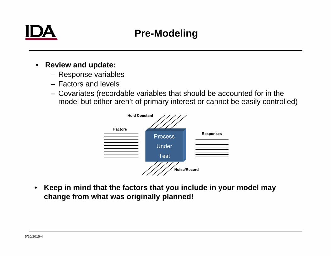
• Review and update: – Response variables – Factors and levels– Covariates (recordable variables that should be accounted for in the

model but either aren’t of primary interest or cannot be easily controlled)

• Keep in mind that the factors that you include in your model may change from what was originally planned!

5/20/2015-5

Pre-Modeling

• Choose the most appropriate distribution for the response variable

– Should have already thought about this notionally– Continuous (e.g. normal, exponential, lognormal, Weibull) vs.

Categorical (e.g. binomial)– Use histograms and QQ-plots to inform decision

5/20/2015-6

Exploratory Data Analysis

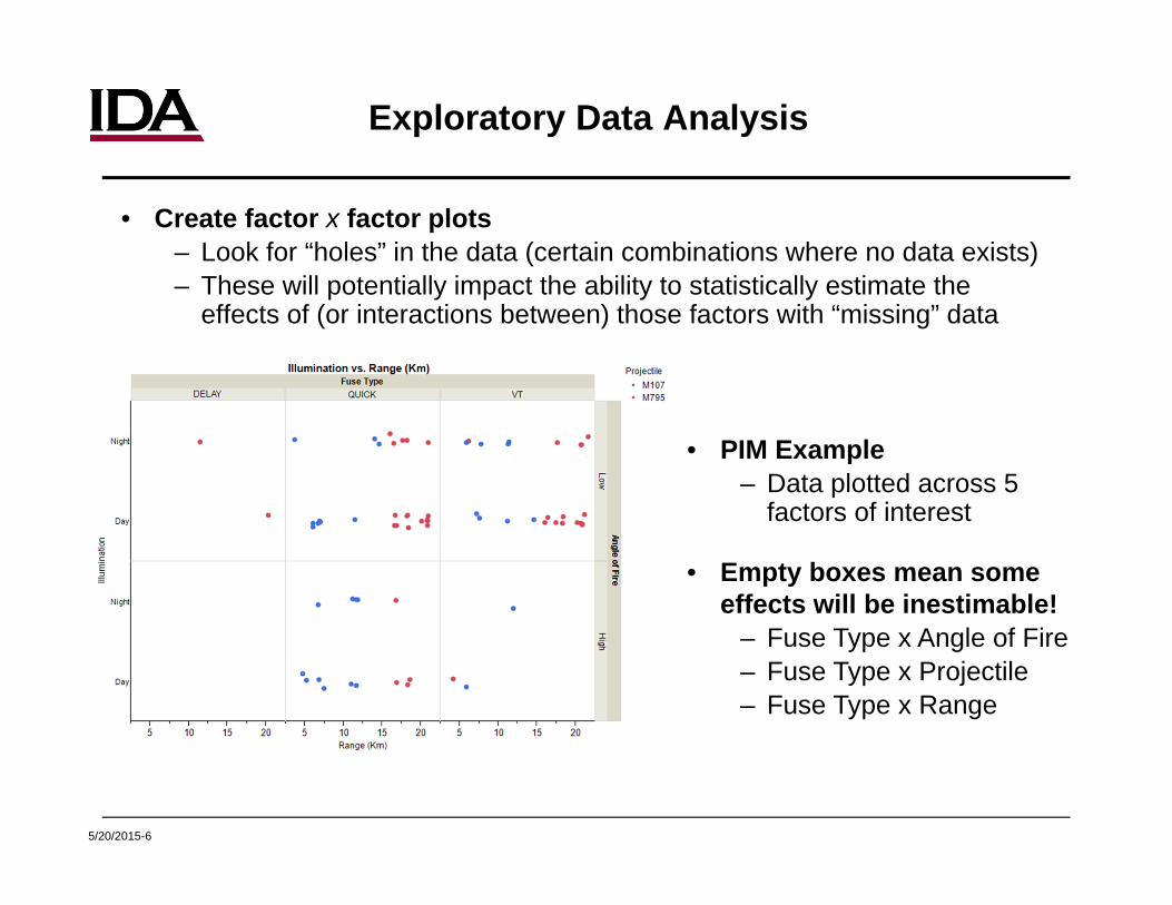
• Create factor x factor plots– Look for “holes” in the data (certain combinations where no data exists)– These will potentially impact the ability to statistically estimate the

effects of (or interactions between) those factors with “missing” data

• PIM Example– Data plotted across 5

factors of interest

• Empty boxes mean some effects will be inestimable!

– Fuse Type x Angle of Fire– Fuse Type x Projectile – Fuse Type x Range

5/20/2015-7

Exploratory Data Analysis (cont.)

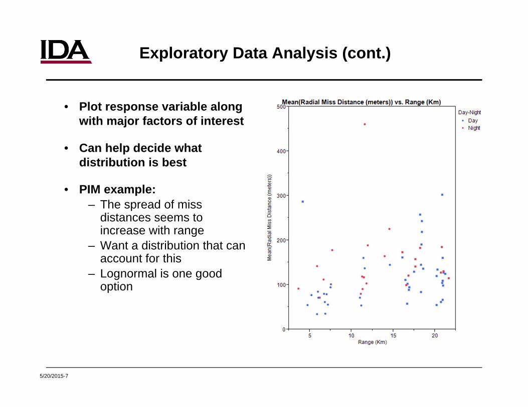
• Plot response variable along with major factors of interest

• Can help decide what distribution is best

• PIM example: – The spread of miss

distances seems to increase with range

– Want a distribution that can account for this

– Lognormal is one good option

5/20/2015-8

Exploratory Data Analysis (cont.)

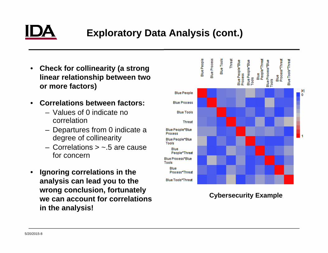
• Check for collinearity (a strong linear relationship between two or more factors)

• Correlations between factors:– Values of 0 indicate no

correlation– Departures from 0 indicate a

degree of collinearity– Correlations > ~.5 are cause

for concern

• Ignoring correlations in the analysis can lead you to the wrong conclusion, fortunately we can account for correlations in the analysis!

Cybersecurity Example

5/20/2015-9

Model Selection Methods

• Forward Selection: Start with nothing but an intercept in the model; test the addition of each variable using a chosen criterion; add the variable (if any) that improves the model the most; repeat until none improve the model

• Backward Selection: Start with all possible variables in the model; test the deletion of each variable using a chosen criterion; remove the variable (if any) that improves the model the most by being deleted; repeat until no further improvement is possible

• Stepwise Selection: A combination of the above methods; test at each stop for variables to be added OR removed

• Automated in some statistical software*

• JMP can perform all 3 types of selection for normally distributed data:Analyze Fit Model Personality = Stepwise (fits all three)

5/20/2015-10

Model Selection Criteria

• p-value– Probability that the effect due to a particular factor (or interaction)

occurred by chance alone– Smaller p-value = stronger effect due to that factor (or interaction)

H0 (Null distribution)

A small p-value means that you are on the tail of a distribution (i.e., very unlikely outcome)

5/20/2015-11

Model Selection Criteria (cont.)

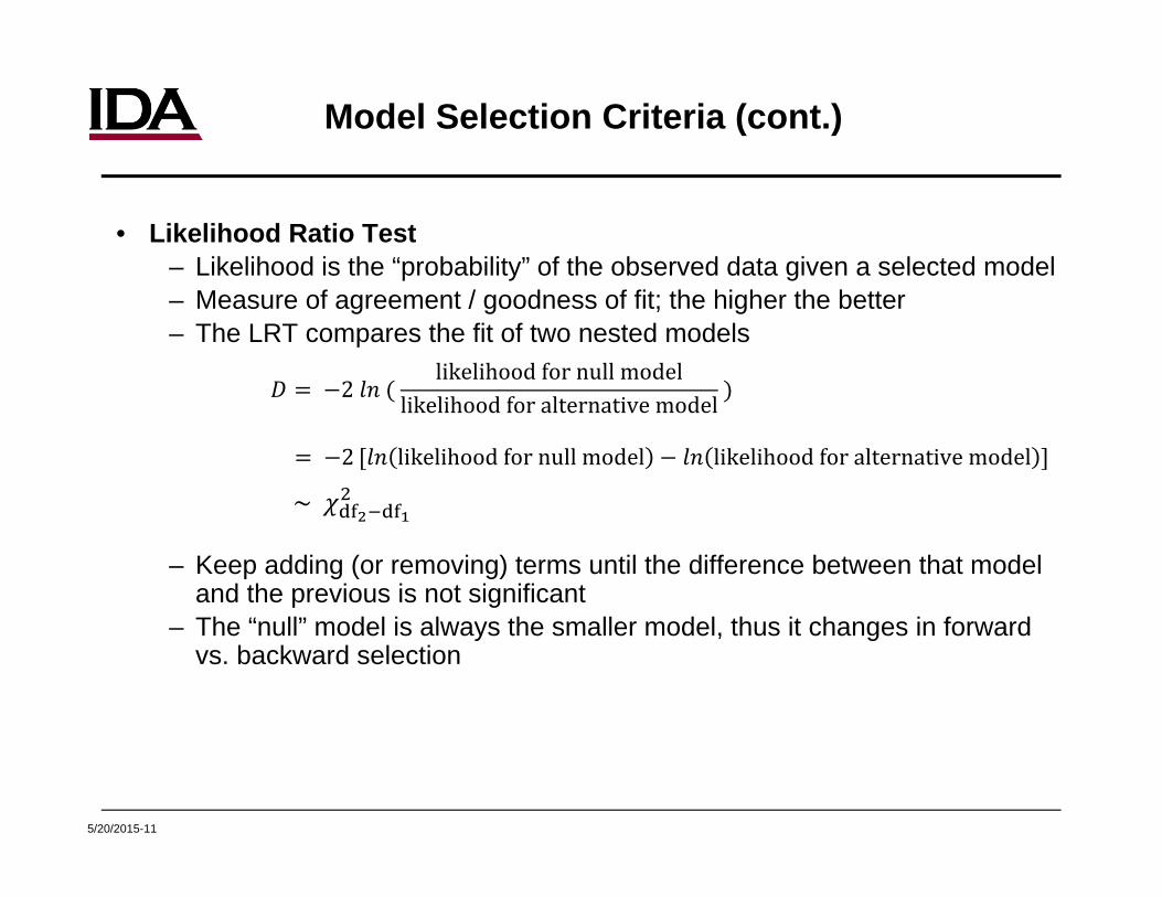
• Likelihood Ratio Test – Likelihood is the “probability” of the observed data given a selected model – Measure of agreement / goodness of fit; the higher the better– The LRT compares the fit of two nested models

2 likelihoodfornullmodel likelihoodforalternativemodel

~

– Keep adding (or removing) terms until the difference between that model and the previous is not significant

– The “null” model is always the smaller model, thus it changes in forward vs. backward selection

2 likelihoodfornullmodel

likelihoodforalternativemodel

5/20/2015-12

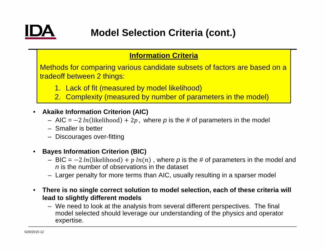
Model Selection Criteria (cont.)

• Akaike Information Criterion (AIC)– AIC = 2 likelihood 2 , where p is the # of parameters in the model – Smaller is better – Discourages over-fitting

• Bayes Information Criterion (BIC)– BIC = 2 likelihood , where p is the # of parameters in the model and

n is the number of observations in the dataset – Larger penalty for more terms than AIC, usually resulting in a sparser model

• There is no single correct solution to model selection, each of these criteria will lead to slightly different models

– We need to look at the analysis from several different perspectives. The final model selected should leverage our understanding of the physics and operator expertise.

Information CriteriaMethods for comparing various candidate subsets of factors are based on a tradeoff between 2 things:

1. Lack of fit (measured by model likelihood)2. Complexity (measured by number of parameters in the model)

5/20/2015-13

Model Validation

• Check Residuals

• Cross Validation

• Compare Model Prediction to Data and/or Non-Parametric Estimates

Remember: “All models are wrong, some models are useful!”

5/20/2015-14

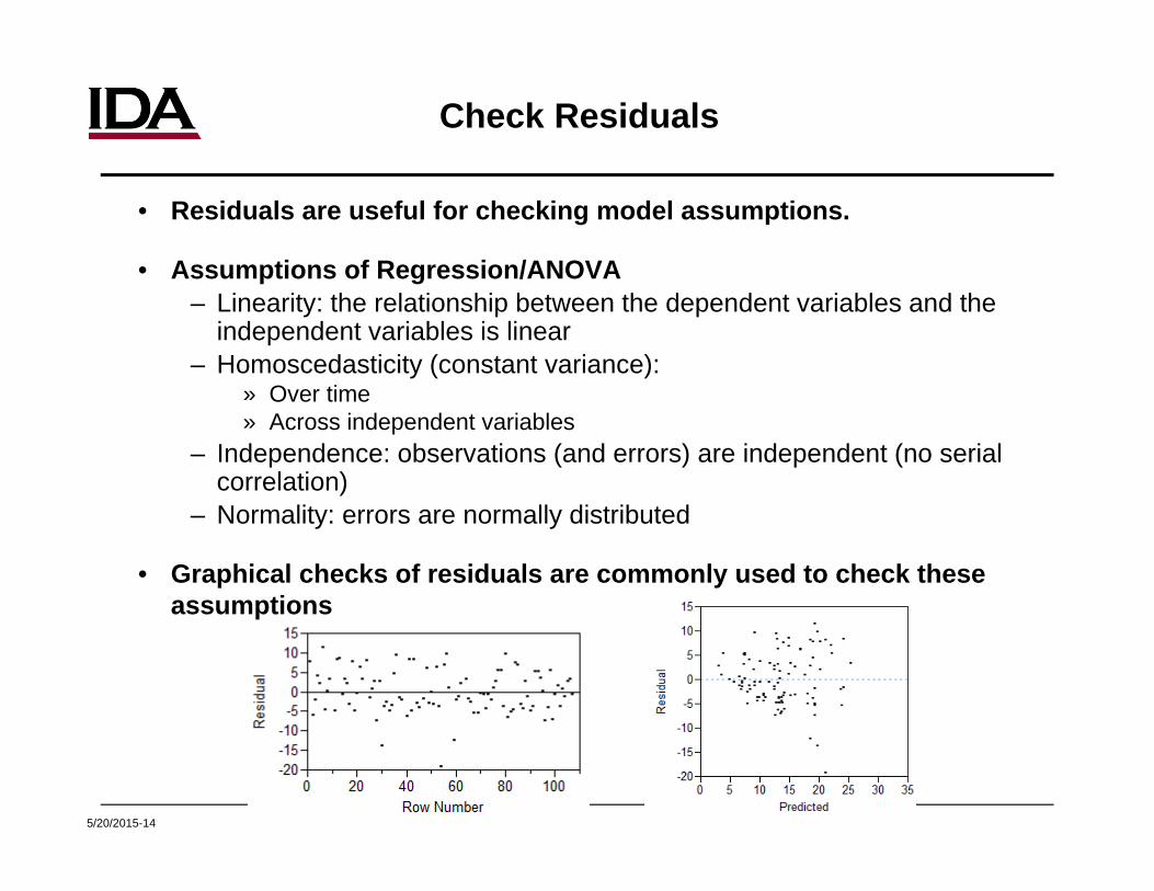
Check Residuals

• Residuals are useful for checking model assumptions.

• Assumptions of Regression/ANOVA– Linearity: the relationship between the dependent variables and the

independent variables is linear– Homoscedasticity (constant variance):

» Over time» Across independent variables

– Independence: observations (and errors) are independent (no serial correlation)

– Normality: errors are normally distributed

• Graphical checks of residuals are commonly used to check these assumptions

5/20/2015-15

Cross-Validation

• Partition a data set into complementary subsets– Perform analysis on one (“training” set)– Validate the analysis on the other (“testing” set)

» Compare the root mean squared errors (RMSE) of the two sets» Testing RMSE will necessarily be higher but difference should not be substantial

– Can perform multiple rounds using different partitions and average the validation results

– Somewhat computationally expensive

• Types of cross-validation:– Even-Odd– k-fold– Leave-one-out

• Requires a certain number of data points (anywhere from 1 more to twice as many as the minimum needed to fit specified model)

– Don’t want to fundamentally change the estimable model by sub-setting the data

– For a small dataset the leave-one-out is probably best

5/20/2015-16

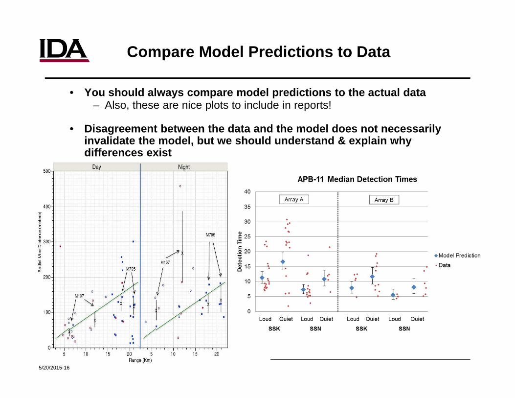
Compare Model Predictions to Data

• You should always compare model predictions to the actual data– Also, these are nice plots to include in reports!

• Disagreement between the data and the model does not necessarily invalidate the model, but we should understand & explain why differences exist

5/20/2015-17

Model Validation Failures

• What do you do if the assumptions are not met?– Consider the impact– Choose a different model that meets the assumptions!

• Typically this involves moving to an advanced methodology such as Generalized Linear Models

• Common Fixes:– Select a different distribution – Lots of T&E response variables

(accuracy, detection range, time to event) do not generally follow a normal distribution. The lognormal distribution is very useful for these problems.

– Add independent variables into variance estimates - note the lognormal distribution will fix some non-constant variance concerns.

– Change relationship of independent variables on model parameters – the link function allows for flexible relationships between independent variables and response variables.

5/20/2015-18

Important Final Points – Model Selection

• Preserve model hierarchy– Always include main effects for factors with interactions included in

the model

• Think about operational/practical significance as well as statistical significance

– Always include factors specifically under investigation– Get SME input

5/20/2015-19

Model Selection Conclusions

• Model selection is a critical part of statistical analysis– Goal is to obtain a sparse model that adequately explains the data– Always think about what you will do with the modeling results

• Get to know your data before fitting models– Choose appropriate distribution of response variable– Create factor plots– Perform collinearity diagnostics

• Various model selection methods and criteria to choose from– There is no ONE correct answer– Use automated procedures in JMP to narrow down terms of interest– Select final model by hand, incorporating SME as appropriate– Consider both statistical and operational significance– Consider the implications for reporting