Copyright © 2005 by the Genetics Society of AmericaDOI: 10.1534/genetics.104.033910

Model Selection in Binary Trait Locus Mapping

Cynthia J. Coffman,*,† R. W. Doerge,‡,§ Katy L. Simonsen,‡ Krista M. Nichols,**Christine K. Duarte,††,‡‡ Russell D. Wolfinger‡‡ and Lauren M. McIntyre†,§,§§,1

*Institute for Clinical and Epidemiological Research Biostatistics Unit, Durham VA Medical Center (152), Durham, North Carolina 27705,†Department of Biostatistics and Bioinformatics, Duke University Medical Center, Durham, North Carolina 27710,

‡Department of Statistics, Purdue University, West Lafayette, Indiana 47907-2068, §Department of Agronomy,Purdue University, West Lafayette, Indiana 47907, §§Computational Genomics, Purdue University,

West Lafayette, Indiana 47907, **Washington State University, School of Biological Sciences,Pullman, Washington 99164, ††Department of Statistics, North Carolina State University,

Raleigh, North Carolina 27695 and ‡‡SAS Institute, Cary, North Carolina 27513

Manuscript received July 23, 2004Accepted for publication March 17, 2005

ABSTRACTQuantitative trait locus (QTL) mapping methodology for continuous normally distributed traits is the

subject of much attention in the literature. Binary trait locus (BTL) mapping in experimental populationshas received much less attention. A binary trait by definition has only two possible values, and the penetranceparameter is restricted to values between zero and one. Due to this restriction, the infinitesimal modelappears to come into play even when only a few loci are involved, making selection of an appropriategenetic model in BTL mapping challenging. We present a probability model for an arbitrary number ofBTL and demonstrate that, given adequate sample sizes, the power for detecting loci is high under a widerange of genetic models, including most epistatic models. A novel model selection strategy based uponthe underlying genetic map is employed for choosing the genetic model. We propose selecting the “best”marker from each linkage group, regardless of significance. This reduces the model space so that an efficientsearch for epistatic loci can be conducted without invoking stepwise model selection. This procedure canidentify unlinked epistatic BTL, demonstrated by our simulations and the reanalysis of Oncorhynchus mykissexperimental data.

STATISTICAL methods for mapping single genes for that estimates the effect for all markers, thus avoidingcontinuous and binary traits in experimental popula- the testing and model selection issues.

tions have advanced significantly in the past few years One approach for reducing the dimensionality of the(Lander and Botstein 1989; Haley and Knott 1992; model space is to locate all QTL that are significantlyZeng 1994; Satagopan et al. 1996; Xu 1996; Xu and associated with the trait, using single-QTL methods, andAtchley 1996; Yi and Xu 2000; McIntyre et al. 2001; then build the multiple-QTL models using only the QTLYi and Xu 2002). Single-gene QTL models have been selected in the single-gene analysis (Kao et al. 1999).expanded to encompass multiple-QTL mapping prob- When all QTL are additive, single-marker analysis is alems by using cofactors or additional markers (Jansen reasonable strategy for identifying QTL (Coffman et al.1993; Zeng 1994; Xu 2003). Multiple-QTL models have 2003). However, epistasis can alter the trait in a mannerbeen developed for both continuous and binary traits that may be difficult to predict (Doerge 2001), thus(Sillanpaa and Arjas 1998; Kao et al. 1999; Zeng et further complicating the model fitting and selectional. 2000; Jannink and Jansen 2001; Sen and Churchill process. Carlborg et al. (2000) proposed a method for2001; Carlborg and Andersson 2002; Yi and Xu 2002; simultaneous mapping of pairwise interacting QTL. InXu 2003) and for discrete traits with multiple observa- addition, Carlborg and Andersson (2002) proposed ation classes (Yi et al. 2004). When attempting to identify forward selection strategy that incorporates a random-multiple QTL for a trait, model selection is a key issue ization test to identify epistatic QTL. Unfortunately, thisas the number of possible models quickly becomes large. approach will miss pairs of loci that are epistatic withoutIn most analyses, the enumeration of all QTL models for a contributing main effect. Holland et al. (2002) per-a data set is possible only when the number of markers is formed a pairwise grid search to identify potential epi-limited. An exception is a recent method (Xu 2003) static loci and then include the most significant pairs

in the “best” single-gene model via a forward stepwiseprocedure. Yi and Xu (2002) proposed a Bayesian

1Corresponding author: Department of Agronomy, 915 W. State St., method to map multiple QTL with pairwise locus epista-Purdue University, West Lafayette, IN 47907.E-mail: lmcintyre@purdue.edu sis. Sen and Churchill (2001) also presented a Bayes-

Genetics 170: 1281–1297 ( July 2005)

1282 C. J. Coffman et al.

ian analysis that implements a strategy similar to that segregation and linkage analysis. The concept of incom-plete penetrance is important, as it underscores theof Jansen (1993), where the QTL problem is dividedcomplexity encountered in analysis of binary traits.into two pieces, detection and then localization. While

As an adaptation of the model in human genetics, andall of these approaches have a common goal, the com-extension of previous work in experimental populationsplexity and computational intensity of many of these(McIntyre et al. 2001), we propose a method to detectapproaches make them difficult to implement. Further-and estimate multiple binary trait loci (BTL). We focusmore, stepwise procedures and pairwise searches do noton the case where penetrance is incomplete and theinvestigate the entire model space and these approachespopulation structure is a backcross or F2 from two inbredhave been shown to fail to identify all possible effectsparents. Using the biological information in the linkagein different applications (Harrell 2001; Burnham andgroups, the model space is reduced by choosing theAnderson 2002).best marker in each linkage group. Consequently, allSearching through the potential models to identifypossible models can be enumerated and stepwise selec-the best model is an active area of statistical researchtion procedures are avoided, which in turn eliminates(Harrell 2001; Burnham and Anderson 2002). Sev-the need for computationally intensive model space ex-eral common criteria are used to judge and compareploration. We use a general probability model based onmodels to select the best model. Due to the large num-classical transmission genetics to develop a likelihoodber of models that may be examined in these analyses,for the binary phenotype (Simonsen 2004) to estimateissues of model selection bias and uncertainty shouldrecombination and penetrance for multiple BTL underbe addressed (Burnham and Anderson 2002). In thecomplex genetic models for an experimental popula-method described by Jansen (1993), the Akaike infor-tion. Regression models are fitted on the basis of thismation criterion (AIC) was used for model selection.likelihood (Haley and Knott 1992; Jansen 1992; Jan-Broman and Speed (2002) reviewed different modelsen and Stam 1994; Whittaker et al. 1996; Thompsonselection criteria for QTL analysis and proposed a crite-1998), using a cell means model parameterizationrion that is a modification of the Bayesian informationrather than the factor effects parameterization (Kutnercriterion (BIC) (Schwarz 1978). Sillanpaa and Coran-et al. 2004). The parameterization in terms of the cellder (2002) gave a general review of model selectionmeans clarifies the identification of epistatic loci.criteria and advocated the Bayesian idea of model aver-

Using simulated data, AIC (Akaike 1973) and BICaging. Others are working on modifications of these(Schwarz 1978) model selection criteria are employedcriteria to improve their performance in the QTL settingand compared for a limited number of markers as well as(Ball 2001; Bogdan et al. 2004; Siegmund 2004). How-in the context of a genome scan. A new SAS procedure,ever, these criteria have not been specifically evaluatedPROC BTL, has been developed and is freely availablefor binary traits.by request (http:www.genomics.purdue.edu/services/In genetic experiments, binary traits often occursoftware/btl). PROC BTL includes model selection forwhen considering characteristics related to susceptibil-a wide range of model selection criteria and implementsity/resistance, sterility/fertility, and mortality/survival.all of the standard model selection techniques includingSen and Churchill (2001) examined binary traits us-the one proposed here. Using PROC BTL, we presenting a generalized linear model framework. Yi and Xua reanalysis of Oncorhynchus mykiss (rainbow or steelhead(2000) proposed a Bayesian method for complex binarytrout) data where single-marker associations of the bi-traits under the threshold model and later extendednary trait, resistance to Ceratomyxa shasta (a myxozoanthis method to map multiple QTL with pairwise locusparasite) (Nichols et al. 2003), suggest that multipleepistasis for binary traits (Yi and Xu 2002). Kilpikariloci may be associated with the resistance. We also findand Sillanpaa (2003) present a multilocus Bayesianevidence for epistatic effects.approach for association mapping that can be used for

binary traits under the threshold or liability model. Thethreshold model is an important quantitative genetic

METHODSmodel. However, the underlying threshold distributionis unobserved (Falconer and Mackay 1996; Lynch A probability model: We denote individual geneticand Walsh 1998), presenting challenges in specifying markers by Mi and BTL by Gi , where i indicates thethe functional form of the threshold model. BTL in map order. We assume a map based on k BTL

In the human genetics literature, binary traits (disease and k markers (M 1G 1M 2G 2 · · · MkGk). The completestatus) are often parameterized in terms of the pene- genotype for all loci is denoted M for markers and Gtrance as well as the physical distance. This model forma- for BTL, and the possible values are described below.tion has been routinely employed for segregation and For a backcross (BC) or F2 population of diploid indi-linkage analysis (Ott 1991; Gauderman and Thomas viduals from a single cross of homozygote inbred par-2001). The value of the penetrance parameter can be ents, there are only two possible alleles for each marker

and/or BTL (denoted by either 1 or 2). In a BC popula-estimated as a part of segregation analysis or in a joint

1283Binary Trait Loci in Experimental Populations

tion with k loci, there are 2k distinct marker classes (i.e., Trait values can be modeled in a variety of ways, andpossible values for M) and 2k distinct BTL genotypes it is useful to consider the penetrance p in the context(i.e., possible values for G), giving a total of 4k possible of standard ANOVA models. For example, consider acombinations of genotypic marker classes (M, G). In an backcross with k � 2. The penetrance parameters areF2 population with phase unknown, there are 3k distinct pg j

, where g j � {11, 12, 21, 22}. Suppose the first digitmarker classes for M and 3k distinct BTL genotypes for of g j is s and the second digit is t. The factor effectsG, resulting in a total of 9k possible combinations of parameterization would be pg j

� � � �s � �t � (��)st ,marker classes and genotypes for (M, G). The number where � and � are the main effects at the two loci andof distinct marker classes or genotypes is represented (��) represents the interaction or epistatic effect andby K from this point forward (i.e., K � 2k for BC and 0 � pg j

, � � 1. The corresponding cell means modelK � 3k for F2). parameterization is pg j

� �st , where the �st are (a func-As in Simonsen (2004), we label and order the K tion of) the cell means. These two model parameteriza-

possible genotypes of markers or BTL as if the genotypes tions are equivalent (Kutner et al. 2004). In the factorwere numerals with one digit per locus, in ascending effects parameterization, absence of epistasis is indi-order. The digit 1 represents the homozygote 1/1 geno- cated by (��)st � 0 and is equivalent to the constrainttype at that locus, 2 is the 1/2 or 2/1 heterozygote, and in the cell means model of p 11 � p 12 � p 21 � p 22 (see3 is the 2/2 homozygote. A genotype for k loci is then Figure 2a). If only locus 1 contributes to the trait, thea k digit number. Thus, with k � 2, a backcross has K � factor effects model constraint is �t � (��)st � 0 while4 possible types {11, 12, 21, 22}, whereas an F2 has K � the cell means model constraint is p 11 � p 12 and p 21 �9 possible genotypes {11, 12, 13, 21, 22, 23, 31, 32, 33}. p 22. Similarly, if only locus 2 is involved, the factor effectsWe label these K values m 1 , . . . , mK or g1 , . . . , gK , model constraint is �s � (��)st � 0 and the cell meansdepending on whether they represent markers or BTL, model constraint is p 11 � p 21 and p 12 � p 22. Epistasisrespectively. The probability distribution of M or G spec- can be presented as a modification of the expectedifies the probabilities of each of these K values and thus segregation ratio with fewer than expected phenotypiccan be written in a vector of length K in the order given. classes observed (Hartl and Jones 2001). Therefore,The joint probability distribution of (M, G) can be writ- the cell means model provides a convenient way often as a K � K matrix Pr(M, G), where the rows index thinking about genetic models, as epistasis is easily de-the marker classes and the columns index the BTL geno- fined as equivalence among penetrance parameters (seetypes. The (i, j)th entry of this matrix represents Pr(M � Figures 2, b–d, and 3).mi , G � g j), where mi and g j each take on the K possi- Simonsen (2004) details the methods for generatingbilities described above. All matrices and vectors refer- the probability model for k BTL in matrix form. Thering to genotypes assume this ordering and indexing. joint probabilities of the BTL genotypes (G), marker

The recombination rate, r i , is the probability that an types (M), and the trait (Y), denoted Pr(Y, M, G), canexchange of genetic material (crossover) occurs be- be expressed in terms of r, , and p and generated fortween the BTL Gi and the marker Mi , where i ranges k BTL for a specified experimental design. Standardfrom 1 to k, where r i � 0 indicates complete association

assumptions such as no selection, interference, or muta-and r i � 0.50 indicates no association between the

tion are made. As an example, the joint probabilitymarker and the BTL. Similarly, the rate of recombina-distribution of a BC for k � 2 is shown in Table 1. Thetion between markers, i , is the probability that an ex-joint probability of every combination of marker andchange of genetic material occurs between marker Mi BTL genotype, Pr(M, G), is computed using the recom-and Mi �1 , where i ranges from 1 to k � 1. If the markerbination probabilities and r. The matrix for the jointmap is assumed known, then the i are fixed.probability of trait, marker, and BTL is then computedThe probability of observing the binary trait is speci-by matrix multiplication Pr(Y, M, G) � Pr(M, G) �fied by K penetrance parameters, p j , which are BernoulliDiag(p), sinceprobabilities representing the probability that a binary

trait Y is present given a specific BTL genotype j (McIn- Pr(Y � 1, M � m i , G � g j) � Pr(Y � 1|G � j)Pr(M � m i , G � g j)tyre et al. 2001). The vector p with entries p j � Pr(Y �

� [Pr(M, G)]i , j � p j .1|G � g j) is of length K, and its j th entry, p j , is thepenetrance parameter for the j th genotype, g j , where j

The joint probability of traits and markers only is usedindexes the possible genotypes in the order explainedfor likelihood calculations as described in the next sec-above. To emphasize the relationship between the geno-tion. This vector of probabilities is computed as Pr(Y,type and the penetrance the notation pg j

may be usedM) � Pr(M, G) � p, where the matrix multiplicationas well as the above p j . Including a penetrance parame-accomplishes the necessary sum over possible geno-ter for each genotype is convenient for visualizing thetypes. Its i th entry isimpact of various genetic models on the parameter

space and is a common tool in human genetics (OttPr(Y � 1, M � m i ) � �

K

j�1

Pr(Y � 1, M � m i , G � g j)1991; Gauderman and Thomas 2001).

1284 C. J. Coffman et al.

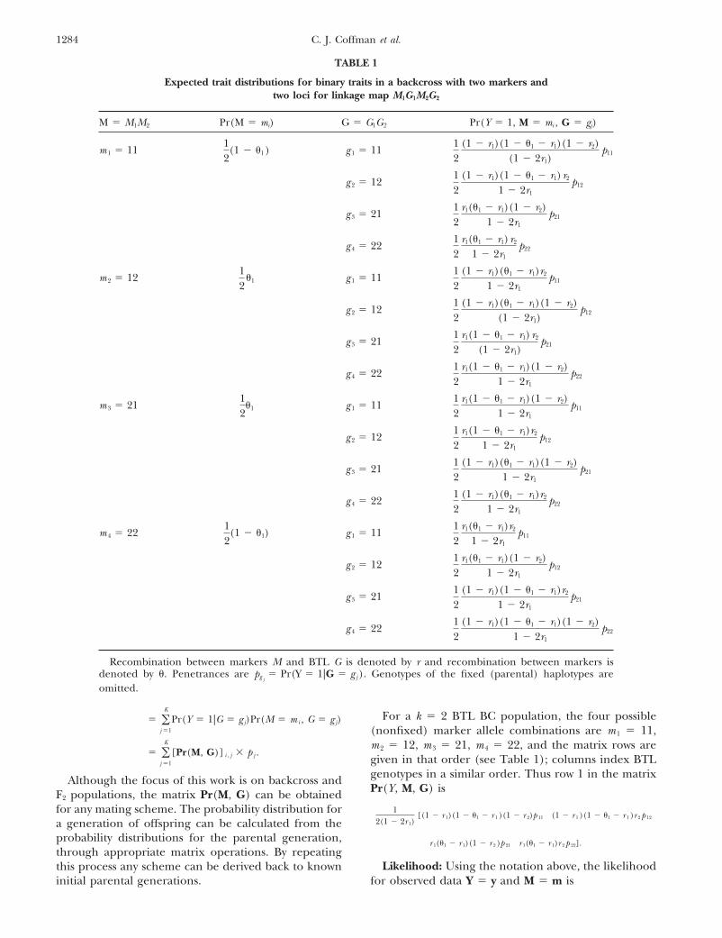
TABLE 1

Expected trait distributions for binary traits in a backcross with two markers andtwo loci for linkage map M1G1M2G2

M � M1M2 Pr(M � mi) G � G1G2 Pr(Y � 1, M � mi , G � gj)

m 1 � 1112(1 � 1 ) g 1 � 11

12

(1 � r1)(1 � 1 � r1)(1 � r2)(1 � 2r1)

p11

g 2 � 1212

(1 � r1)(1 � 1 � r1) r2

1 � 2r1

p12

g 3 � 2112

r1(1 � r1)(1 � r2)1 � 2r1

p21

g 4 � 2212

r1(1 � r1) r2

1 � 2r1

p22

m 2 � 1212

1 g 1 � 1112

(1 � r1)(1 � r1)r2

1 � 2r1

p11

g 2 � 1212

(1 � r1)(1 � r1)(1 � r2)(1 � 2r1)

p12

g 3 � 2112

r1(1 � 1 � r1) r2

(1 � 2r1)p21

g 4 � 2212

r1(1 � 1 � r1)(1 � r2)1 � 2r1

p22

m 3 � 2112

1 g 1 � 1112

r1(1 � 1 � r1)(1 � r2)1 � 2r1

p11

g 2 � 1212

r1(1 � 1 � r1)r2

1 � 2r1

p12

g 3 � 2112

(1 � r1)(1 � r1)(1 � r2)1 � 2r1

p21

g 4 � 2212

(1 � r1)(1 � r1)r2

1 � 2r1

p22

m 4 � 2212(1 � 1) g 1 � 11

12

r1(1 � r1)r2

1 � 2r1

p11

g 2 � 1212

r1(1 � r1)(1 � r2)1 � 2r1

p12

g 3 � 2112

(1 � r1)(1 � 1 � r1)r2

1 � 2r1

p21

g 4 � 2212

(1 � r1)(1 � 1 � r1)(1 � r2)1 � 2r1

p22

Recombination between markers M and BTL G is denoted by r and recombination between markers isdenoted by . Penetrances are pg j

� Pr(Y � 1|G � g j ). Genotypes of the fixed (parental) haplotypes areomitted.

For a k � 2 BTL BC population, the four possible� �K

j �1

Pr(Y � 1|G � g j)Pr(M � m i , G � g j)(nonfixed) marker allele combinations are m 1 � 11,m 2 � 12, m 3 � 21, m 4 � 22, and the matrix rows are

� �K

j �1

[Pr(M, G)] i , j � p j . given in that order (see Table 1); columns index BTLgenotypes in a similar order. Thus row 1 in the matrixAlthough the focus of this work is on backcross andPr(Y, M, G) isF2 populations, the matrix Pr(M, G) can be obtained

for any mating scheme. The probability distribution for 12(1 � 2r 1)

[(1 � r 1)(1 � 1 � r 1 )(1 � r 2)p 11 (1 � r 1 )(1 � 1 � r 1 )r 2 p 12

a generation of offspring can be calculated from theprobability distributions for the parental generation, r 1(1 � r 1)(1 � r 2 )p 21 r 1(1 � r 1)r 2 p 22].through appropriate matrix operations. By repeating

Likelihood: Using the notation above, the likelihoodthis process any scheme can be derived back to knowninitial parental generations. for observed data Y � y and M � m is

1285Binary Trait Loci in Experimental Populations

L(r, , p) � Pr(Y � y, M � m|r, , p). The resulting system of equations is linear in p and �and nonlinear in r. Since there are K equations and

This likelihood can also be written in terms of the K � k unknowns, the system is underdetermined. Formarker class means, as follows. any fixed r, however, there is a unique and easily ob-

The expected marker class means are denoted by the tained solution for p, and, furthermore, the values arevector � whose ith entry, i , is the marker class mean subject to constraints, namely 0 � r i � 0.5 and 0 �for marker class i, namely pg j

� 1. We use a grid search to step through the intervalof possible r values to obtain sets of solutions for p.

i � Pr(Y � 1|M � mi) �Pr(Y � 1, M � mi)

Pr(M � mi) In some cases, solutions do not satisfy the biologicalconstraint 0 � pg j

� 1 for all g j and can be discarded,or simply if a filter on the resulting estimates is desired. In other

situations, the correct values of some penetrances mayPr(Y � 1, M � mi) � i Pr(M � mi).be known or separately estimable from previous experi-

The component of the likelihood for a single observa- mental generations. In these cases estimates can be fur-tion with Y � 1 and M � mi is the ith entry of the vector ther constrained. For example, if parental penetrancesPr(Y � 1, M). Since Pr(Y � 0|M � mi) � 1 � i , we are known, the values of r and p that minimize thehave Pr(Y � 0, M � mi) � (1 � i)Pr(M � mi). Note distance between the known values of the parental pene-that � is a function of r, , and p, while Pr(M) is a trances and their estimates can be chosen. Other possi-function of only. Therefore, the likelihood for a single ble solutions to this problem exist; for example, nonlin-observation from marker class i is ear programming methods may be applied. We initially

explored applying nonlinear programming (NLP) tech-niques; however, estimation for k loci was not easilyL(r, , p) � �i Pr(M � mi), Y � 1

(1 � i)Pr(M � mi), Y � 0.implemented.

Premodeling strategy: Generally, mapping data con-Suppose in a given sample there are ni individuals insist of a set of markers and a trait evaluation for eachmarker class i, of whom zi exhibit Y � 1, and ni � ziindividual in the experimental population. The numberexhibit Y � 0. Then the likelihood can be written as aof BTL that can be fit to the data depends on the sampleproduct over marker classes:size (i.e., the degrees of freedom). If the set of markers

L(r, , p) � �K

i �1

(i Pr(M � m i ))z i((1 � i )Pr(M � m i ))n i�z i (1) is relatively large, as is generally the case, enumeratingall possible models becomes impossible, and we needsome methodology for reducing the model space. We� �

K

i �1

z ii (1 � i )n i�z i(Pr(M � m i ))n i. (2)

propose to limit the model space explored by choosingone marker per linkage group. Another strategy forMaximum-likelihood estimates for marker classreducing the model space is to limit multiple-markermeans: Using this likelihood, the maximum-likelihoodmodels to only markers that are significantly associatedestimates (MLEs) for the marker class means can bewith the trait on the basis of single-locus models (Kaoobtained by maximizing model 1 to obtain estimates ofet al. 1999; Carlborg and Andersson 2002). However,the binomial proportions i � z i/ni for i � 1 . . . K.this strategy might miss markers without strong mainThe marker class means i are easily estimated fromeffects that are otherwise involved in epistasis. Anotherthe data. To estimate penetrance p and recombinationstrategy is to examine all possible pairs of loci (Hollandr, we exploit the relationship between p and �. Let � �et al. 2002; Yi and Xu 2002) to reduce the chance ofDiag(Pr(M)) such that ��1 � Diag(1/Pr(M � m 1), . . . ,missing a locus with primarily epistatic effect. While1/Pr(M � mK)). Then Pr(G|M) � ��1Pr(M, G) so thatit is possible to look at all possible pairs of markers,Pr(G|M)�1 � Pr(M, G)�1� can be calculated. In termsexamining all possible triplets and quadruplets quicklyof this quantity, the relationship between p and � isbecomes impractical. Additionally, significant model se-thuslection bias and uncertainty is introduced (Burnham

� � Pr(Y � 1|M) � Pr(G|M) � p, and Anderson 2002; Bogdan et al. 2004).To avoid stepwise procedures and selection methodsso that

based upon pairwise relationships it has been proposedp � [Pr(G|M)]�1 � �. that the relationships among predictor variables can

be exploited to reduce model space (Harrell 2001).This gives p as a function of r, , and �. If the markerFortunately, markers have an inherent relationship amongmap is known [and hence Pr(M) is known], p is a func-themselves based on genetic distance and form groupstion of only r and �.of correlated covariates known as linkage groups. ByEstimation: To estimate recombination (r) and pene-selecting the best marker (or interval) from each linkagetrance (p) parameters the invariance property of MLEsgroup, the dimensionality of the problem is greatly re-can be invoked (Casella and Berger 1990). Thusduced. The criteria for choosing the best among themarkers for a linkage group are also possible to explore.p � [Pr(G|M)]�1|r �r � �. (3)

1286 C. J. Coffman et al.

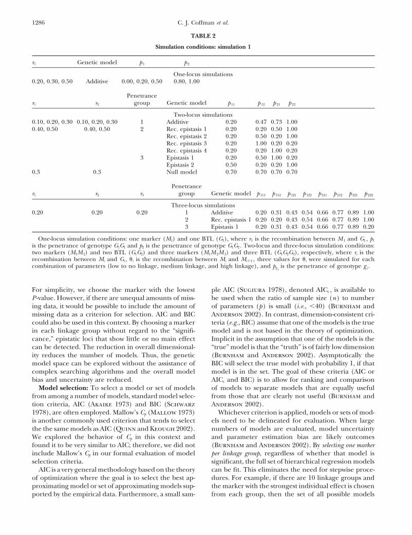
TABLE 2

Simulation conditions: simulation 1

r1 Genetic model p 1 p 2

One-locus simulations0.20, 0.30, 0.50 Additive 0.00, 0.20, 0.50 0.80, 1.00

Penetrancer1 r2 group Genetic model p 11 p 12 p 21 p 22

Two-locus simulations0.10, 0.20, 0.30 0.10, 0.20, 0.30 1 Additive 0.20 0.47 0.73 1.000.40, 0.50 0.40, 0.50 2 Rec. epistasis 1 0.20 0.20 0.50 1.00

Rec. epistasis 2 0.20 0.50 0.20 1.00Rec. epistasis 3 0.20 1.00 0.20 0.20Rec. epistasis 4 0.20 0.20 1.00 0.20

3 Epistasis 1 0.20 0.50 1.00 0.20Epistasis 2 0.50 0.20 0.20 1.00

0.3 0.3 Null model 0.70 0.70 0.70 0.70

Penetrancer1 r2 r3 group Genetic model p 111 p 112 p 121 p 122 p 211 p 212 p 221 p 222

Three-locus simulations0.20 0.20 0.20 1 Additive 0.20 0.31 0.43 0.54 0.66 0.77 0.89 1.00

2 Rec. epistasis 1 0.20 0.20 0.43 0.54 0.66 0.77 0.89 1.003 Epistasis 1 0.20 0.31 0.43 0.54 0.66 0.77 0.89 0.20

One-locus simulation conditions: one marker (M1) and one BTL (G1), where r1 is the recombination between M 1 and G1 , p1

is the penetrance of genotype G1G1 and p2 is the penetrance of genotype G1G2 . Two-locus and three-locus simulation conditions:two markers (M1M 2) and two BTL (G1G2) and three markers (M1M 2M 3) and three BTL (G1G2G3), respectively, where ri is therecombination between Mi and Gi , i is the recombination between Mi and Mi�1 , three values for i were simulated for eachcombination of parameters (low to no linkage, medium linkage, and high linkage), and pg j

is the penetrance of genotype g j .

For simplicity, we choose the marker with the lowest ple AIC (Sugiura 1978), denoted AICc, is available tobe used when the ratio of sample size (n) to numberP -value. However, if there are unequal amounts of miss-

ing data, it would be possible to include the amount of of parameters (p) is small (i.e., �40) (Burnham andAnderson 2002). In contrast, dimension-consistent cri-missing data as a criterion for selection. AIC and BIC

could also be used in this context. By choosing a marker teria (e.g., BIC) assume that one of the models is the truemodel and is not based in the theory of optimization.in each linkage group without regard to the “signifi-

cance,” epistatic loci that show little or no main effect Implicit in the assumption that one of the models is the“true” model is that the “truth” is of fairly low dimensioncan be detected. The reduction in overall dimensional-

ity reduces the number of models. Thus, the genetic (Burnham and Anderson 2002). Asymptotically theBIC will select the true model with probability 1, if thatmodel space can be explored without the assistance of

complex searching algorithms and the overall model model is in the set. The goal of these criteria (AIC orAICc and BIC) is to allow for ranking and comparisonbias and uncertainty are reduced.

Model selection: To select a model or set of models of models to separate models that are equally usefulfrom those that are clearly not useful (Burnham andfrom among a number of models, standard model selec-

tion criteria, AIC (Akaike 1973) and BIC (Schwarz Anderson 2002).Whichever criterion is applied, models or sets of mod-1978), are often employed. Mallow’s Cp (Mallow 1973)

is another commonly used criterion that tends to select els need to be delineated for evaluation. When largenumbers of models are evaluated, model uncertaintythe the same models as AIC (Quinn and Keough 2002).

We explored the behavior of Cp in this context and and parameter estimation bias are likely outcomes(Burnham and Anderson 2002). By selecting one markerfound it to be very similar to AIC; therefore, we did not

include Mallow’s Cp in our formal evaluation of model per linkage group, regardless of whether that model issignificant, the full set of hierarchical regression modelsselection criteria.

AIC is a very general methodology based on the theory can be fit. This eliminates the need for stepwise proce-dures. For example, if there are 10 linkage groups andof optimization where the goal is to select the best ap-

proximating model or set of approximating models sup- the marker with the strongest individual effect is chosenfrom each group, then the set of all possible modelsported by the empirical data. Furthermore, a small sam-

1287Binary Trait Loci in Experimental Populations

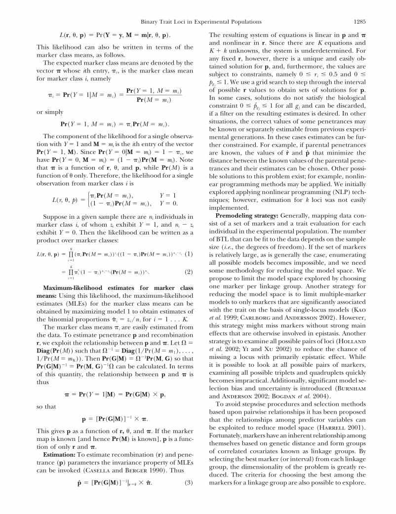
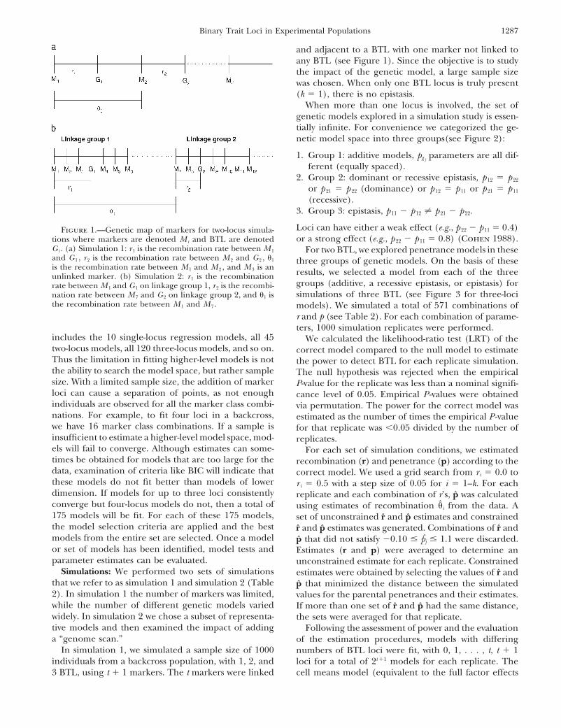
and adjacent to a BTL with one marker not linked toany BTL (see Figure 1). Since the objective is to studythe impact of the genetic model, a large sample sizewas chosen. When only one BTL locus is truly present(k � 1), there is no epistasis.

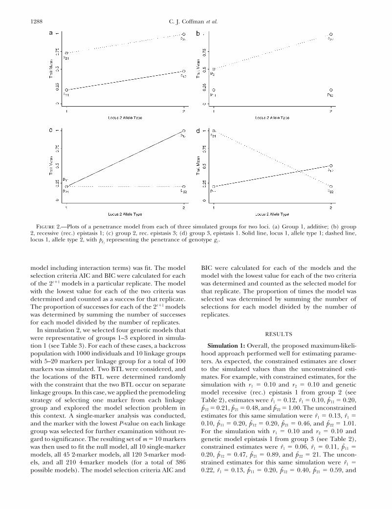
When more than one locus is involved, the set ofgenetic models explored in a simulation study is essen-tially infinite. For convenience we categorized the ge-netic model space into three groups(see Figure 2):

1. Group 1: additive models, pg jparameters are all dif-

ferent (equally spaced).2. Group 2: dominant or recessive epistasis, p 12 � p 22

or p 21 � p 22 (dominance) or p 12 � p 11 or p 21 � p 11

(recessive).3. Group 3: epistasis, p 11 � p 12 � p 21 � p 22.

Loci can have either a weak effect (e.g., p 22 � p 11 � 0.4)Figure 1.—Genetic map of markers for two-locus simula-or a strong effect (e.g., p 22 � p 11 � 0.8) (Cohen 1988).tions where markers are denoted M i and BTL are denoted

G i . (a) Simulation 1: r 1 is the recombination rate between M 1 For two BTL, we explored penetrance models in theseand G 1 , r 2 is the recombination rate between M 2 and G 2 , 1 three groups of genetic models. On the basis of theseis the recombination rate between M 1 and M 2 , and M 3 is an results, we selected a model from each of the threeunlinked marker. (b) Simulation 2: r 1 is the recombination

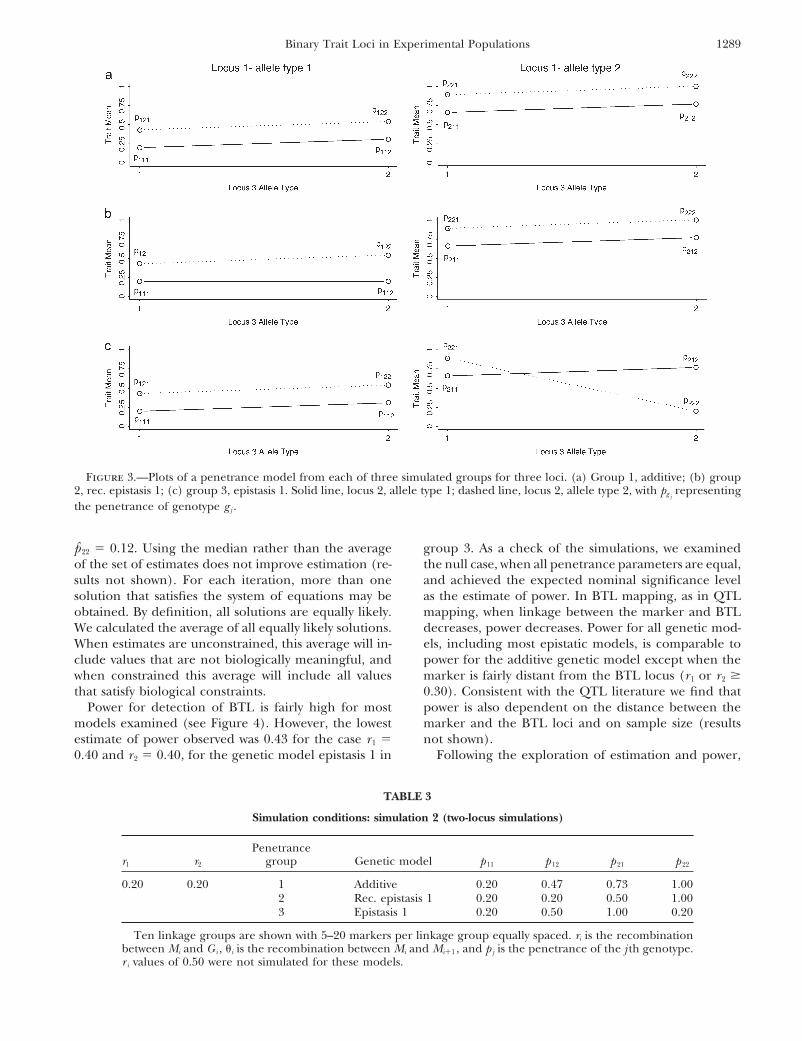
groups (additive, a recessive epistasis, or epistasis) forrate between M 1 and G 1 on linkage group 1, r 2 is the recombi-simulations of three BTL (see Figure 3 for three-locination rate between M 7 and G 2 on linkage group 2, and 1 is

the recombination rate between M 1 and M 7 . models). We simulated a total of 571 combinations ofr and p (see Table 2). For each combination of parame-ters, 1000 simulation replicates were performed.

includes the 10 single-locus regression models, all 45 We calculated the likelihood-ratio test (LRT) of thetwo-locus models, all 120 three-locus models, and so on. correct model compared to the null model to estimateThus the limitation in fitting higher-level models is not the power to detect BTL for each replicate simulation.the ability to search the model space, but rather sample The null hypothesis was rejected when the empiricalsize. With a limited sample size, the addition of marker P-value for the replicate was less than a nominal signifi-loci can cause a separation of points, as not enough cance level of 0.05. Empirical P -values were obtainedindividuals are observed for all the marker class combi- via permutation. The power for the correct model wasnations. For example, to fit four loci in a backcross, estimated as the number of times the empirical P -valuewe have 16 marker class combinations. If a sample is for that replicate was �0.05 divided by the number ofinsufficient to estimate a higher-level model space, mod- replicates.els will fail to converge. Although estimates can some- For each set of simulation conditions, we estimatedtimes be obtained for models that are too large for the recombination (r) and penetrance (p) according to thedata, examination of criteria like BIC will indicate that correct model. We used a grid search from r i � 0.0 tothese models do not fit better than models of lower r i � 0.5 with a step size of 0.05 for i � 1–k. For eachdimension. If models for up to three loci consistently replicate and each combination of r’s, p was calculatedconverge but four-locus models do not, then a total of using estimates of recombination i from the data. A175 models will be fit. For each of these 175 models, set of unconstrained r and p estimates and constrainedthe model selection criteria are applied and the best r and p estimates was generated. Combinations of r andmodels from the entire set are selected. Once a model p that did not satisfy �0.10 � pj � 1.1 were discarded.or set of models has been identified, model tests and Estimates (r and p) were averaged to determine anparameter estimates can be evaluated. unconstrained estimate for each replicate. Constrained

Simulations: We performed two sets of simulations estimates were obtained by selecting the values of r andthat we refer to as simulation 1 and simulation 2 (Table p that minimized the distance between the simulated2). In simulation 1 the number of markers was limited, values for the parental penetrances and their estimates.while the number of different genetic models varied If more than one set of r and p had the same distance,widely. In simulation 2 we chose a subset of representa- the sets were averaged for that replicate.tive models and then examined the impact of adding Following the assessment of power and the evaluationa “genome scan.” of the estimation procedures, models with differing

In simulation 1, we simulated a sample size of 1000 numbers of BTL loci were fit, with 0, 1, . . . , t, t � 1individuals from a backcross population, with 1, 2, and loci for a total of 2t �1 models for each replicate. The

cell means model (equivalent to the full factor effects3 BTL, using t � 1 markers. The t markers were linked

1288 C. J. Coffman et al.

Figure 2.—Plots of a penetrance model from each of three simulated groups for two loci. (a) Group 1, additive; (b) group2, recessive (rec.) epistasis 1; (c) group 2, rec. epistasis 3; (d) group 3, epistasis 1. Solid line, locus 1, allele type 1; dashed line,locus 1, allele type 2, with pg j

representing the penetrance of genotype g j .

model including interaction terms) was fit. The model BIC were calculated for each of the models and themodel with the lowest value for each of the two criteriaselection criteria AIC and BIC were calculated for each

of the 2t �1 models in a particular replicate. The model was determined and counted as the selected model forthat replicate. The proportion of times the model waswith the lowest value for each of the two criteria was

determined and counted as a success for that replicate. selected was determined by summing the number ofselections for each model divided by the number ofThe proportion of successes for each of the 2t �1 models

was determined by summing the number of successes replicates.for each model divided by the number of replicates.

In simulation 2, we selected four genetic models thatRESULTS

were representative of groups 1–3 explored in simula-tion 1 (see Table 3). For each of these cases, a backcross Simulation 1: Overall, the proposed maximum-likeli-

hood approach performed well for estimating parame-population with 1000 individuals and 10 linkage groupswith 5–20 markers per linkage group for a total of 100 ters. As expected, the constrained estimates are closer

to the simulated values than the unconstrained esti-markers was simulated. Two BTL were considered, andthe locations of the BTL were determined randomly mates. For example, with constrained estimates, for the

simulation with r 1 � 0.10 and r 2 � 0.10 and geneticwith the constraint that the two BTL occur on separatelinkage groups. In this case, we applied the premodeling model recessive (rec.) epistasis 1 from group 2 (see

Table 2), estimates were r 1 � 0.12, r 1 � 0.10, p 11 � 0.20,strategy of selecting one marker from each linkagegroup and explored the model selection problem in p 12 � 0.21, p 21 � 0.48, and p 22 � 1.00. The unconstrained

estimates for this same simulation were r 1 � 0.13, r 1 �this context. A single-marker analysis was conducted,and the marker with the lowest P -value on each linkage 0.10, p 11 � 0.20, p 12 � 0.20, p 21 � 0.46, and p 22 � 1.01.

For the simulation with r 1 � 0.10 and r 2 � 0.10 andgroup was selected for further examination without re-gard to significance. The resulting set of m � 10 markers genetic model epistasis 1 from group 3 (see Table 2),

constrained estimates were r 1 � 0.06, r 1 � 0.11, p 11 �was then used to fit the null model, all 10 single-markermodels, all 45 2-marker models, all 120 3-marker mod- 0.20, p 12 � 0.47, p 21 � 0.89, and p 22 � 21. The uncon-

strained estimates for this same simulation were r 1 �els, and all 210 4-marker models (for a total of 386possible models). The model selection criteria AIC and 0.22, r 1 � 0.13, p 11 � 0.20, p 12 � 0.40, p 21 � 0.59, and

1289Binary Trait Loci in Experimental Populations

Figure 3.—Plots of a penetrance model from each of three simulated groups for three loci. (a) Group 1, additive; (b) group2, rec. epistasis 1; (c) group 3, epistasis 1. Solid line, locus 2, allele type 1; dashed line, locus 2, allele type 2, with pg j

representingthe penetrance of genotype g j .

p 22 � 0.12. Using the median rather than the average group 3. As a check of the simulations, we examinedthe null case, when all penetrance parameters are equal,of the set of estimates does not improve estimation (re-

sults not shown). For each iteration, more than one and achieved the expected nominal significance levelas the estimate of power. In BTL mapping, as in QTLsolution that satisfies the system of equations may be

obtained. By definition, all solutions are equally likely. mapping, when linkage between the marker and BTLdecreases, power decreases. Power for all genetic mod-We calculated the average of all equally likely solutions.

When estimates are unconstrained, this average will in- els, including most epistatic models, is comparable topower for the additive genetic model except when theclude values that are not biologically meaningful, and

when constrained this average will include all values marker is fairly distant from the BTL locus (r 1 or r 2 0.30). Consistent with the QTL literature we find thatthat satisfy biological constraints.

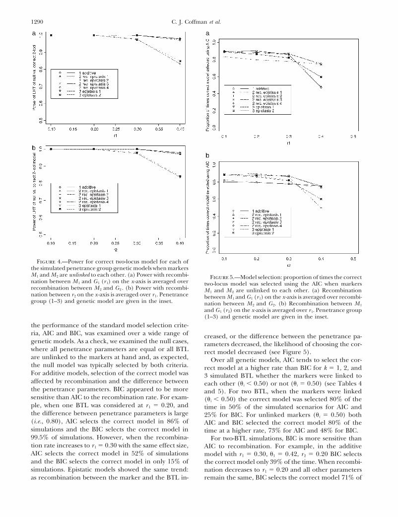
Power for detection of BTL is fairly high for most power is also dependent on the distance between themarker and the BTL loci and on sample size (resultsmodels examined (see Figure 4). However, the lowest

estimate of power observed was 0.43 for the case r 1 � not shown).Following the exploration of estimation and power,0.40 and r 2 � 0.40, for the genetic model epistasis 1 in

TABLE 3

Simulation conditions: simulation 2 (two-locus simulations)

Penetrancer1 r2 group Genetic model p 11 p 12 p 21 p 22

0.20 0.20 1 Additive 0.20 0.47 0.73 1.002 Rec. epistasis 1 0.20 0.20 0.50 1.003 Epistasis 1 0.20 0.50 1.00 0.20

Ten linkage groups are shown with 5–20 markers per linkage group equally spaced. ri is the recombinationbetween Mi and G i , i is the recombination between Mi and Mi�1 , and p j is the penetrance of the j th genotype.r i values of 0.50 were not simulated for these models.

1290 C. J. Coffman et al.

Figure 4.—Power for correct two-locus model for each ofthe simulated penetrance group genetic models when markersM 1 and M 2 are unlinked to each other. (a) Power with recombi- Figure 5.—Model selection: proportion of times the correctnation between M 1 and G 1 (r 1) on the x -axis is averaged over two-locus model was selected using the AIC when markersrecombination between M 2 and G 2 . (b) Power with recombi- M 1 and M 2 are unlinked to each other. (a) Recombinationnation between r 2 on the x -axis is averaged over r 1. Penetrance between M 1 and G 1 (r 1) on the x -axis is averaged over recombi-group (1–3) and genetic model are given in the inset. nation between M 2 and G 2. (b) Recombination between M 1

and G 1 (r 2) on the x -axis is averaged over r 1. Penetrance group(1–3) and genetic model are given in the inset.

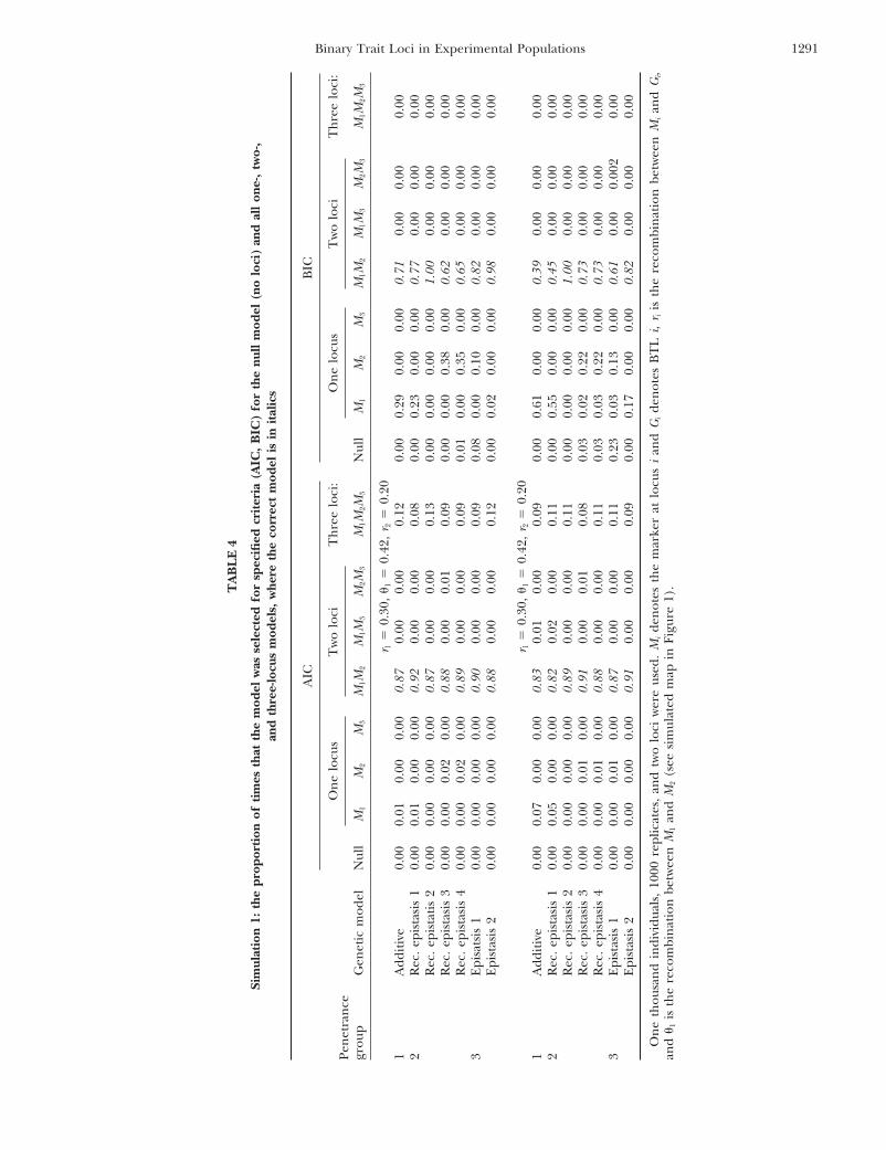
the performance of the standard model selection crite-ria, AIC and BIC, was examined over a wide range of creased, or the difference between the penetrance pa-genetic models. As a check, we examined the null cases, rameters decreased, the likelihood of choosing the cor-where all penetrance parameters are equal or all BTL rect model decreased (see Figure 5).are unlinked to the markers at hand and, as expected, Over all genetic models, AIC tends to select the cor-the null model was typically selected by both criteria. rect model at a higher rate than BIC for k � 1, 2, andFor additive models, selection of the correct model was 3 simulated BTL whether the markers were linked toaffected by recombination and the difference between each other (i � 0.50) or not (i � 0.50) (see Tables 4the penetrance parameters. BIC appeared to be more and 5). For two BTL, when the markers were linkedsensitive than AIC to the recombination rate. For exam- (i � 0.50) the correct model was selected 80% of theple, when one BTL was considered at r 1 � 0.20, and time in 50% of the simulated scenarios for AIC andthe difference between penetrance parameters is large 25% for BIC. For unlinked markers (i � 0.50) both(i.e., 0.80), AIC selects the correct model in 86% of AIC and BIC selected the correct model 80% of thesimulations and the BIC selects the correct model in time at a higher rate, 73% for AIC and 48% for BIC.99.5% of simulations. However, when the recombina- For two-BTL simulations, BIC is more sensitive thantion rate increases to r 1 � 0.30 with the same effect size, AIC to recombination. For example, in the additiveAIC selects the correct model in 52% of simulations model with r 1 � 0.30, 1 � 0.42, r 2 � 0.20 BIC selectsand the BIC selects the correct model in only 15% of the correct model only 39% of the time. When recombi-simulations. Epistatic models showed the same trend: nation decreases to r 1 � 0.20 and all other parameters

remain the same, BIC selects the correct model 71% ofas recombination between the marker and the BTL in-

1291Binary Trait Loci in Experimental Populations

TA

BL

E4

Sim

ulat

ion

1:th

epr

opor

tion

ofti

mes

that

the

mod

elw

asse

lect

edfo

rsp

ecifi

edcr

iter

ia(A

IC,

BIC

)fo

rth

enu

llm

odel

(no

loci

)an

dal

lon

e-,

two-

,an

dth

ree-

locu

sm

odel

s,w

here

the

corr

ect

mod

elis

init

alic

s

AIC

BIC

On

elo

cus

Tw

olo

ciT

hre

elo

ci:

On

elo

cus

Tw

olo

ciT

hre

elo

ci:

Pen

etra

nce

grou

pG

enet

icm

odel

Nul

lM

1M

2M

3M

1M2

M1M

3M

2M3

M1M

2M3

Nul

lM

1M

2M

3M

1M2

M1M

3M

2M3

M1M

2M3

r 1�

0.30

,

1�

0.42

,r 2

�0.

201

Add

itiv

e0.

000.

010.

000.

000.

870.

000.

000.

120.

000.

290.

000.

000.

710.

000.

000.

002

Rec

.ep

ista

sis

10.

000.

010.

000.

000.

920.

000.

000.

080.

000.

230.

000.

000.

770.

000.

000.

00R

ec.

epis

tati

s2

0.00

0.00

0.00

0.00

0.87

0.00

0.00

0.13

0.00

0.00

0.00

0.00

1.00

0.00

0.00

0.00

Rec

.ep

ista

sis

30.

000.

000.

020.

000.

880.

000.

010.

090.

000.

000.

380.

000.

620.

000.

000.

00R

ec.

epis

tasi

s4

0.00

0.00

0.02

0.00

0.89

0.00

0.00

0.09

0.01

0.00

0.35

0.00

0.65

0.00

0.00

0.00

3E

pisa

tsis

10.

000.

000.

000.

000.

900.

000.

000.

090.

080.

000.

100.

000.

820.

000.

000.

00E

pist

asis

20.

000.

000.

000.

000.

880.

000.

000.

120.

000.

020.

000.

000.

980.

000.

000.

00

r 1�

0.30

,

1�

0.42

,r 2

�0.

201

Add

itiv

e0.

000.

070.

000.

000.

830.

010.

000.

090.

000.

610.

000.

000.

390.

000.

000.

002

Rec

.ep

ista

sis

10.

000.

050.

000.

000.

820.

020.

000.

110.

000.

550.

000.

000.

450.

000.

000.

00R

ec.

epis

tasi

s2

0.00

0.00

0.00

0.00

0.89

0.00

0.00

0.11

0.00

0.00

0.00

0.00

1.00

0.00

0.00

0.00

Rec

.ep

ista

sis

30.

000.

000.

010.

000.

910.

000.

010.

080.

030.

020.

220.

000.

730.

000.

000.

00R

ec.

epis

tasi

s4

0.00

0.00

0.01

0.00

0.88

0.00

0.00

0.11

0.03

0.03

0.22

0.00

0.73

0.00

0.00

0.00

3E

pist

asis

10.

000.

000.

010.

000.

870.

000.

000.

110.

230.

030.

130.

000.

610.

000.

002

0.00

Epi

stas

is2

0.00

0.00

0.00

0.00

0.91

0.00

0.00

0.09

0.00

0.17

0.00

0.00

0.82

0.00

0.00

0.00

On

eth

ousa

nd

indi

vidu

als,

1000

repl

icat

es,

and

two

loci

wer

eus

ed.

Mi

den

otes

the

mar

ker

atlo

cus

ian

dG

ide

not

esB

TL

i,r i

isth

ere

com

bin

atio

nbe

twee

nM

ian

dG

i,an

d

1is

the

reco

mbi

nat

ion

betw

een

M1

and

M2

(see

sim

ulat

edm

apin

Figu

re1)

.

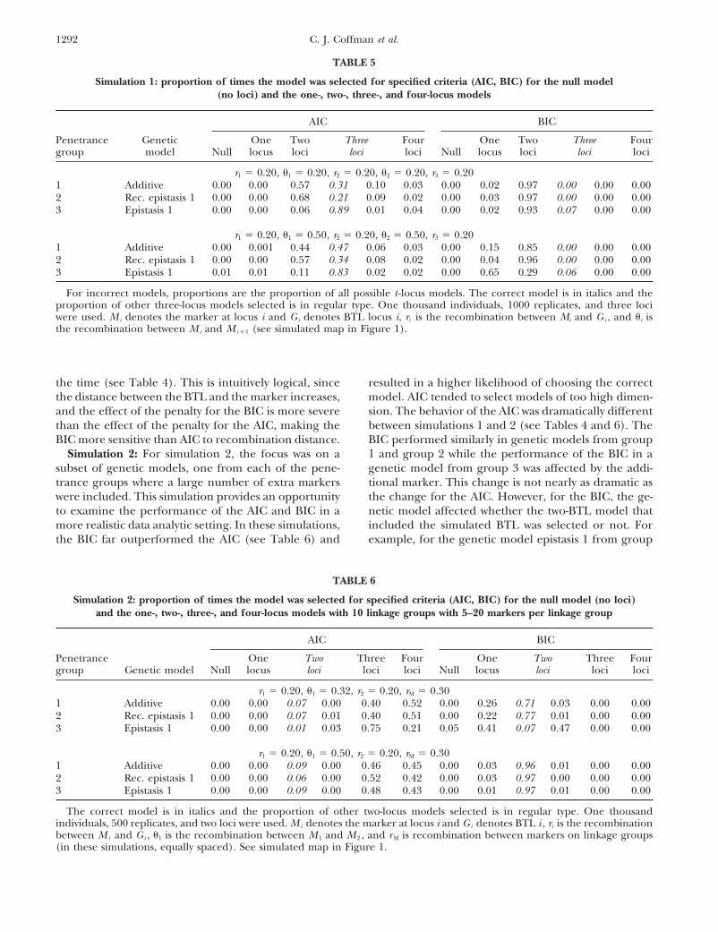
1292 C. J. Coffman et al.

TABLE 5

Simulation 1: proportion of times the model was selected for specified criteria (AIC, BIC) for the null model(no loci) and the one-, two-, three-, and four-locus models

AIC BIC

Penetrance Genetic One Two Three Four One Two Three Fourgroup model Null locus loci loci loci Null locus loci loci loci

r1 � 0.20, 1 � 0.20, r2 � 0.20, 2 � 0.20, r3 � 0.201 Additive 0.00 0.00 0.57 0.31 0.10 0.03 0.00 0.02 0.97 0.00 0.00 0.002 Rec. epistasis 1 0.00 0.00 0.68 0.21 0.09 0.02 0.00 0.03 0.97 0.00 0.00 0.003 Epistasis 1 0.00 0.00 0.06 0.89 0.01 0.04 0.00 0.02 0.93 0.07 0.00 0.00

r1 � 0.20, 1 � 0.50, r2 � 0.20, 2 � 0.50, r3 � 0.201 Additive 0.00 0.001 0.44 0.47 0.06 0.03 0.00 0.15 0.85 0.00 0.00 0.002 Rec. epistasis 1 0.00 0.00 0.57 0.34 0.08 0.02 0.00 0.04 0.96 0.00 0.00 0.003 Epistasis 1 0.01 0.01 0.11 0.83 0.02 0.02 0.00 0.65 0.29 0.06 0.00 0.00

For incorrect models, proportions are the proportion of all possible t -locus models. The correct model is in italics and theproportion of other three-locus models selected is in regular type. One thousand individuals, 1000 replicates, and three lociwere used. M i denotes the marker at locus i and G i denotes BTL locus i, ri is the recombination between Mi and G i , and i isthe recombination between M i and M i �1 (see simulated map in Figure 1).

the time (see Table 4). This is intuitively logical, since resulted in a higher likelihood of choosing the correctmodel. AIC tended to select models of too high dimen-the distance between the BTL and the marker increases,

and the effect of the penalty for the BIC is more severe sion. The behavior of the AIC was dramatically differentbetween simulations 1 and 2 (see Tables 4 and 6). Thethan the effect of the penalty for the AIC, making the

BIC more sensitive than AIC to recombination distance. BIC performed similarly in genetic models from group1 and group 2 while the performance of the BIC in aSimulation 2: For simulation 2, the focus was on a

subset of genetic models, one from each of the pene- genetic model from group 3 was affected by the addi-tional marker. This change is not nearly as dramatic astrance groups where a large number of extra markers

were included. This simulation provides an opportunity the change for the AIC. However, for the BIC, the ge-netic model affected whether the two-BTL model thatto examine the performance of the AIC and BIC in a

more realistic data analytic setting. In these simulations, included the simulated BTL was selected or not. Forexample, for the genetic model epistasis 1 from groupthe BIC far outperformed the AIC (see Table 6) and

TABLE 6

Simulation 2: proportion of times the model was selected for specified criteria (AIC, BIC) for the null model (no loci)and the one-, two-, three-, and four-locus models with 10 linkage groups with 5–20 markers per linkage group

AIC BIC

Penetrance One Two Three Four One Two Three Fourgroup Genetic model Null locus loci loci loci Null locus loci loci loci

r1 � 0.20, 1 � 0.32, r2 � 0.20, rM � 0.301 Additive 0.00 0.00 0.07 0.00 0.40 0.52 0.00 0.26 0.71 0.03 0.00 0.002 Rec. epistasis 1 0.00 0.00 0.07 0.01 0.40 0.51 0.00 0.22 0.77 0.01 0.00 0.003 Epistasis 1 0.00 0.00 0.01 0.03 0.75 0.21 0.05 0.41 0.07 0.47 0.00 0.00

r1 � 0.20, 1 � 0.50, r2 � 0.20, rM � 0.301 Additive 0.00 0.00 0.09 0.00 0.46 0.45 0.00 0.03 0.96 0.01 0.00 0.002 Rec. epistasis 1 0.00 0.00 0.06 0.00 0.52 0.42 0.00 0.03 0.97 0.00 0.00 0.003 Epistasis 1 0.00 0.00 0.09 0.00 0.48 0.43 0.00 0.01 0.97 0.01 0.00 0.00

The correct model is in italics and the proportion of other two-locus models selected is in regular type. One thousandindividuals, 500 replicates, and two loci were used. M i denotes the marker at locus i and G i denotes BTL i , ri is the recombinationbetween M i and G i , 1 is the recombination between M 1 and M 2 , and r M is recombination between markers on linkage groups(in these simulations, equally spaced). See simulated map in Figure 1.

1293Binary Trait Loci in Experimental Populations

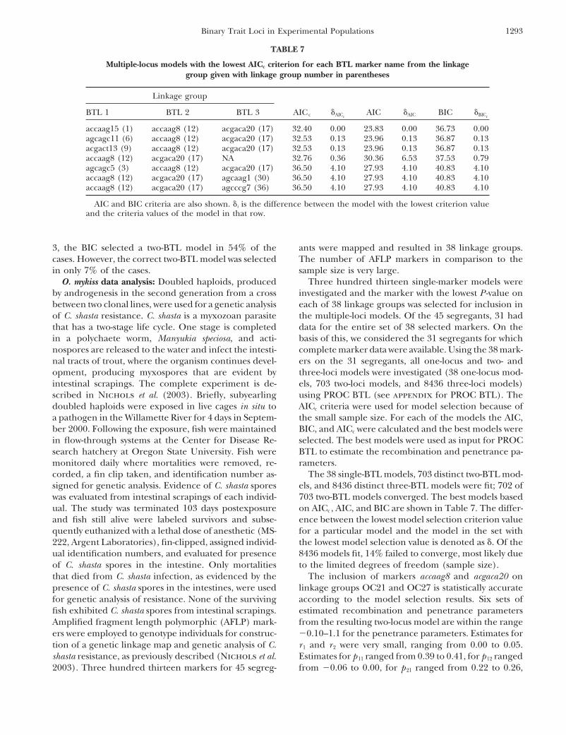
TABLE 7

Multiple-locus models with the lowest AICc criterion for each BTL marker name from the linkagegroup given with linkage group number in parentheses

Linkage group

BTL 1 BTL 2 BTL 3 AIC c �AICcAIC �AIC BIC �BICc

accaag15 (1) accaag8 (12) acgaca20 (17) 32.40 0.00 23.83 0.00 36.73 0.00agcagc11 (6) accaag8 (12) acgaca20 (17) 32.53 0.13 23.96 0.13 36.87 0.13acgact13 (9) accaag8 (12) acgaca20 (17) 32.53 0.13 23.96 0.13 36.87 0.13accaag8 (12) acgaca20 (17) NA 32.76 0.36 30.36 6.53 37.53 0.79agcagc5 (3) accaag8 (12) acgaca20 (17) 36.50 4.10 27.93 4.10 40.83 4.10accaag8 (12) acgaca20 (17) agcaag1 (30) 36.50 4.10 27.93 4.10 40.83 4.10accaag8 (12) acgaca20 (17) agcccg7 (36) 36.50 4.10 27.93 4.10 40.83 4.10

AIC and BIC criteria are also shown. �i is the difference between the model with the lowest criterion valueand the criteria values of the model in that row.

3, the BIC selected a two-BTL model in 54% of the ants were mapped and resulted in 38 linkage groups.The number of AFLP markers in comparison to thecases. However, the correct two-BTL model was selected

in only 7% of the cases. sample size is very large.Three hundred thirteen single-marker models wereO. mykiss data analysis: Doubled haploids, produced

by androgenesis in the second generation from a cross investigated and the marker with the lowest P -value oneach of 38 linkage groups was selected for inclusion inbetween two clonal lines, were used for a genetic analysis

of C. shasta resistance. C. shasta is a myxozoan parasite the multiple-loci models. Of the 45 segregants, 31 haddata for the entire set of 38 selected markers. On thethat has a two-stage life cycle. One stage is completed

in a polychaete worm, Manyukia speciosa, and acti- basis of this, we considered the 31 segregants for whichcomplete marker data were available. Using the 38 mark-nospores are released to the water and infect the intesti-

nal tracts of trout, where the organism continues devel- ers on the 31 segregants, all one-locus and two- andthree-loci models were investigated (38 one-locus mod-opment, producing myxospores that are evident by

intestinal scrapings. The complete experiment is de- els, 703 two-loci models, and 8436 three-loci models)using PROC BTL (see appendix for PROC BTL). Thescribed in Nichols et al. (2003). Briefly, subyearling

doubled haploids were exposed in live cages in situ to AICc criteria were used for model selection because ofthe small sample size. For each of the models the AIC,a pathogen in the Willamette River for 4 days in Septem-

ber 2000. Following the exposure, fish were maintained BIC, and AICc were calculated and the best models wereselected. The best models were used as input for PROCin flow-through systems at the Center for Disease Re-

search hatchery at Oregon State University. Fish were BTL to estimate the recombination and penetrance pa-rameters.monitored daily where mortalities were removed, re-

corded, a fin clip taken, and identification number as- The 38 single-BTL models, 703 distinct two-BTL mod-els, and 8436 distinct three-BTL models were fit; 702 ofsigned for genetic analysis. Evidence of C. shasta spores

was evaluated from intestinal scrapings of each individ- 703 two-BTL models converged. The best models basedon AICc, AIC, and BIC are shown in Table 7. The differ-ual. The study was terminated 103 days postexposure

and fish still alive were labeled survivors and subse- ence between the lowest model selection criterion valuefor a particular model and the model in the set withquently euthanized with a lethal dose of anesthetic (MS-

222, Argent Laboratories), fin-clipped, assigned individ- the lowest model selection value is denoted as �. Of the8436 models fit, 14% failed to converge, most likely dueual identification numbers, and evaluated for presence

of C. shasta spores in the intestine. Only mortalities to the limited degrees of freedom (sample size).The inclusion of markers accaag8 and acgaca20 onthat died from C. shasta infection, as evidenced by the

presence of C. shasta spores in the intestines, were used linkage groups OC21 and OC27 is statistically accurateaccording to the model selection results. Six sets offor genetic analysis of resistance. None of the surviving

fish exhibited C. shasta spores from intestinal scrapings. estimated recombination and penetrance parametersfrom the resulting two-locus model are within the rangeAmplified fragment length polymorphic (AFLP) mark-

ers were employed to genotype individuals for construc- �0.10–1.1 for the penetrance parameters. Estimates forr 1 and r 2 were very small, ranging from 0.00 to 0.05.tion of a genetic linkage map and genetic analysis of C.

shasta resistance, as previously described (Nichols et al. Estimates for p 11 ranged from 0.39 to 0.41, for p 12 rangedfrom �0.06 to 0.00, for p 21 ranged from 0.22 to 0.26,2003). Three hundred thirteen markers for 45 segreg-

1294 C. J. Coffman et al.

and for p 22 ranged from 1.03 to 1.08. The small sample models in our simulations, performance of the BIC de-creases while the AIC remains approximately the same.combined with the observation that none of the individ-

uals with allele 1 of marker accaag8 and allele 2 of Examining these models closely, we see that the varyingdifficulty can be explained by considering the pene-marker acgaca20 survived made the addition of a third

locus unwise from an estimation perspective (marker trance parameters as mixing parameters and examiningthe relative effect size difference between the loci.class means 11 � 0.097, 12 � 0.00, 21 � 0.065, and

22 � 0.26). The goals and results of simulation 2 are markedlydifferent. Unlinked BTL are easier to identify thanlinked BTL simply because they are considered inde-

DISCUSSIONpendently. This effect can be diminished by expandingthe model search space once the best model or set ofThis article presents a general likelihood for multiple

BTL. The likelihood formulation presented here is simi- models has been selected from among the restrictedset. Examining models that increase the number of locilar to that employed by Yi and Xu (2002) with the

exception that their liability function is replaced by our by adding loci linked to loci already included in thebest model will allow for additional opportunities tosingle penetrance parameter. Since the estimation of

the liability function is computationally challenging, detect linked BTL, while still restricting the model spaceto a manageable number of loci.and the methods employed are often sensitive to the

choice of this function, our approach greatly simplifies The comparison between simulation 1 and simulation2 underscores the main differences among the two crite-the likelihood and corresponding evaluation process.

By choosing one marker per linkage group in a premod- ria examined. The AIC selects the best “approximating”model for the data, and in cases where few markers areeling step, we greatly reduce the model space and avoid

stepwise model selection and complicated searching al- available, these are often the correct selections. In thecase of a genome scan, this will result in the additiongorithms. Rather than choosing only markers significant

in the single-locus models or examining all possible of loci, particularly in the case of linked BTL. The BICwill more often choose the right model among a largepairs of loci, the relationships (linkage) between mark-

ers can be exploited to choose the best locus for each set of models when the true model is of relatively lowdimension and is included in the set of models to select.linkage group. This reduces the model space and the

impact of model selection upon the subsequent estima- In the case of the genome scan the BIC has a largerpenalty and thus more often chooses a model of appro-tion and testing procedures.

While we focus on selection of a single marker in a priate or lower dimension. However, when the numberof loci examined is limited, the penalty for the BIClinkage group, the idea of reducing the marker set can

be applied more broadly. For example, in cases where forces models of too low a dimension to be selected.Bogdan et al. (2004) propose a modification to thethe linkage group may itself be large, the best marker

for some fixed genetic distance may be chosen. Alterna- BIC that accommodates the dimensionality of the BTLapplication and that could be extended to apply heretively, two or three markers per linkage group may be

selected. and perhaps mitigate this finding.In the analysis of the O. mykiss there were a fair num-In the first simulation, epistatic models are easier to

select correctly than the strictly additive model. Initially ber of missing marker data. For the purposes of compari-son of the techniques explored in this article, the maxi-this was a surprising result but when a fully additive

model is considered, with the restriction of the parame- mum set of complete data was chosen. This is becauseone of the main assumptions of both AIC and BIC is ater space for the penetrance parameters, 0 � p j � 1,

the marginal effect of any one locus is small. This is constant sample size. Changing the sample size betweenmodels will adversely affect the model selection processwhat is predicted by Fisher’s infinitesimal model with a

large number of loci. The extension of this idea will be and because of the penalty term, especially with respectto the BIC, changing the criterion between models willtrue in quantitative traits as well if the range of the trait

values is restricted. In contrast, epistasis restricts the result in changes in the formulation of the likelihoodfunction. As an additional criterion in the premodelingparameters such that several of the penetrances are

equal. The consequence of this is larger marginal effects strategy, one might group markers in the linkage groupinto a set of best markers and then among those markersof individual loci. This underscores the importance of

fitting models that include epistatic terms as well as choose the marker (or interval) with the most completedata. Furthermore, methods that impute the value ofmain effects.

The effect of linkage between the BTL changes the missing marker data show promise to reduce the impactof missing marker data. In addition to the missingperformance of the selection criteria. For additive mod-

els with recessive epistasis (groups 1 and 2) the influence marker data, the sample size for these data is exceed-ingly small. The size is so small that inferences drawnof linkage among BTL improves model selection. For

epistasis that considers two loci in model selection it is from these data are by necessity suggestive, and furtherexperiments would need to be done to make any defini-more difficult when BTL are linked and for the recessive

1295Binary Trait Loci in Experimental Populations

ping based on model selection: approximate analysis using thetive conclusions. In general, the small sample correctionBayesian information criterion. Genetics 159: 1351–1364.

of the AIC (e.g., AICc) is considered preferable com- Bogdan, M., J. K. Ghosh and R. W. Doerge, 2004 Modifying theSchwarz Bayesian information criterion to locate multiple inter-pared to invoking the asymptotic behavior of the AICacting quantitative trait loci. Genetics 167: 989–999.and BIC. Of note is the fact that the three criteria se-

Broman, K. W., and T. P. Speed, 2002 A model selection approachlected the same set of models with similar ranking for the identification of quantitative trait loci in experimental

crosses. J. R. Stat. Soc. Ser. B 64: 641–656.among models. Examining the set of models that haveBurnham, K. P., and D. R. Anderson, 2002 Model Selection andsimilar AIC, AICc, and BIC values, it is apparent that

Multimodel Inference: A Practical Information-Theoretic Approach, Ed.linkage groups OC21 and OC27 are a common theme. 2. Springer, Berlin/Heidelberg, Germany/New York.

Carlborg, O., and L. Andersson, 2002 Use of randomization test-This is particularly interesting as linkage group OC27ing to detect multiple epistatic QTL. Genet. Res. 79: 175–184.had no significant BTL in the single-marker analysis.

Carlborg, O., L. Andersson and B. Kinghorn, 2000 The use ofThis points to the possible identification of an epistatic a genetic algorithm for simultaneous mapping of multiple inter-

acting quantitative trait loci. Genetics 155: 2003–2010.effect in the absence of a significant main effect for thatCasella, G., and R. L. Berger, 1990 Statistical Inference. Wads-locus. Additional BTL may be located on linkage groups

worth & Brooks/Cole, Pacific Grove, CA.OC7,OC13,OC15,OC30,OC-a, and OC-b, but the joint Coffman, C. J., R. W. Doerge, M. L. Wayne and L. M. McIntyre,

2003 Intersection tests for single marker QTL analysis can beestimation of parameters in models of this dimensionmore powerful than two marker QTL analysis. BMC Genet. 4:for this small sample size is not recommended.10 (http://www.biomedcentral.com/1471-2156/4/10).

The typical treatment of binary traits has restricted Cohen, J., 1988 Statistical Power Analysis for the Behavioral Sciences, Ed.2. Lawrence Earlbaum Associates, Hilldale, NJ.the use of these data to single-marker analyses. What

Doerge, R. W., 2001 Mapping and analysis of quantitative trait lociwe propose here is to acknowledge the full depth ofin experimental populations. Nat. Rev. Genet. 3: 43–52.

binary traits by allowing a modeling strategy that accom- Falconer, D. S., and T. F. C. Mackay, 1996 Introduction to Quantita-tive Genetics, Ed. 4. Longman, Essex, UK.modates the potential for epistasis while being aware of

Gauderman, W. J., and D. C. Thomas, 2001 The role of interactingthe computational challenges that are present in high-determinants in the localization of genes, pp. 393–412 in Advances

dimensional model spaces. By changing the parameter- in Genetics, Vol. 42: Genetic Dissection of Complex Traits, edited byD. C. Rao and M. A. Province. Academic Press, San Diego.ization of the likelihood function to include marker

Haley, C., and S. Knott, 1992 A simple regression method forclass means, the estimation of penetrance can be ob-mapping quantitative trait loci in line crosses using flanking mark-

tained. We implement a grid search technique to obtain ers. Heredity 69: 315–324.Harrell, F. E., 2001 Regression Modeling Strategies With Applicationsthe solution. There are other potential solutions to this

to Linear Models, Logistic Regression, and Survival Analysis. Springer,system of nonlinear equations, but these present a com-New York.

plex numerical problem that is a subject of future work. Hartl, D., and E. Jones, 2001 Genetics: Analysis of Genes and Genomes.Jones & Bartlett, Sudbury, MA.We have provided an easily accessible procedure in SAS

Holland, J. B., V. A. Portyanko, D. L. Hoffman and M. Lee, 2002that allows multiple-BTL mapping under a wide rangeGenomic regions controlling vernalization and photoperiod re-

of strategies for the purpose of providing a tool that sponses in oat. Theor. Appl. Genet. 105: 113–126.Jannink, J., and R. Jansen, 2001 Mapping epistatic quantitative traitscientists can use with ease and flexibility.

loci with one-dimensional genome searches. Genetics 157: 445–Even though specific model selection criteria (BIC,454.

AIC, and AICc) are employed to evaluate the models Jansen, R. C., 1992 A general mixture model for mapping quantita-tive trait loci by using molecular markers. Theor. Appl. Genet.that result from the model selection procedure pro-85: 252–260.posed, other criteria could easily be used in conjunction

Jansen, R. C., 1993 Interval mapping of multiple quantitative traitwith the premodeling strategy proposed. The optimal loci. Genetics 135: 205–211.

Jansen, R. C., and P. Stam, 1994 High resolution of quantitativecriterion for model selection is an open and excitingtraits into multiple loci via interval mapping. Genetics 136: 1447–area of research. In the situation presented here the1455.

issue is further complicated by constraining the parame- Kao, C.-H., Z-B. Zeng and R. D. Teasdale, 1999 Multiple intervalmapping for quantitative trait loci. Genetics 152: 1203–1216.ter space, which in turn makes proper evaluation of

Kilpikari, R., and M. J. Sillanpaa, 2003 Bayesian analysis of multilo-the correct model choice more difficult than it maycus association in quantitative and qualitative traits. Genet. Epide-

otherwise appear. miol. 25: 122–135.Kutner, M. H., C. J. Nachtsheim, J. Neter and W. Li, 2004 AppliedThis work is supported by National Science Foundation grant DBI

Linear Statistical Models, Ed. 5. McGraw-Hill Irwin, New York.98-08026/00-96044 (L.M.M., C.J.C., R.W.D.), National Institutes ofLander, E. S., and D. Botstein, 1989 Mapping Mendelian factors

Health grants NIA-AG16996 (L.M.M.) and 2G12RR003048 (L.M.M.), underlying quantitative traits using RFLP linkage maps. GeneticsU.S. Department of Agriculture (USDA) grant 98-35300-6173 121: 185–199.(R.W.D.), USDA-Initiative for Future Agriculture and Food Systems Lynch, M., and B. Walsh, 1998 Genetics and Analysis of Quantitativegrant N0014-94-1-0318 (R.W.D., L.M.M.), and a Veterans Affairs Traits. Sinauer Associates, Sunderland, MA.

Mallow, C. L., 1973 Some comments on Cp . Technometrics 12:Health Services Research Postdoctoral Fellowship (C.J.C.).591–612.

McIntyre, L. M., C. J. Coffman and R. W. Doerge, 2001 Detectionand localization of a single binary trait locus in experimentalpopulations. Genet. Res. 78: 79–92.LITERATURE CITED

Nichols, K., J. Bartholomew and G. H. Thorgaard, 2003 Map-ping multiple genetic loci associated with Ceratomyxa shasta resis-Akaike, H., 1973 Information theory as an extension, pp. 267–281

in Second International Symposium on Information Theory, edited by tance in Oncorhynchus mykiss. Dis. Aquat. Org. 56 (2): 145–154.Ott, J., 1991 Analysis of Human Genetic Linkage. Johns Hopkins Uni-B. Petrov and F. Csaki. Akademiai Kiado, Budapest.

Ball, R. D., 2001 Bayesian methods for quantitative trait loci map- versity Press, Baltimore.

1296 C. J. Coffman et al.

Quinn, G. P., and M. J. Keough, 2002 Experimental Design and Data Thompson, E. A., 1998 Inferring gene ancestry: estimating genedescent. Int. Stat. Rev. 66: 29–40.Analysis for Biologists. Cambridge University Press, Cambridge/

Whittaker, J. C., R. Thompson and P. M. Visscher, 1996 On theLondon/New York.mapping of QTL by regression of phenotypes on marker type.Satagopan, J. M., B. S. Yandell, M. A. Newton and T. C. Osborn,Heredity 77: 23–32.1996 A Bayesian approach to detect quantitative trait loci Mar-

Xu, S., 1996 Computation of the full likelihood function for estimat-kov chain Monte Carlo. Genetics 144: 805–816.ing variance at a quantitative trait locus. Genetics 144: 1951–1960.Schwarz, S. L., 1978 Estimating the dimension of a model. Ann.

Xu, S., 2003 Estimating polygenic effects using markers of the entireStat. 6: 461–464.genome. Genetics 163: 789–801.Sen, S., and G. A. Churchill, 2001 A statistical framework for quan-

Xu, S., and W. R. Atchley, 1996 Mapping quantitative trait locititative trait mapping. Genetics 159: 371–387.for complex binary diseases using line crosses. Genetics 143:Siegmund, D. O., 2004 Model selection in irregular problems: appli-1417–1424.cations to mapping quantitative trait loci. Biometrika 91: 785–800.

Yi, N., and S. Xu, 2000 Bayesian mapping of quantitative trait lociSillanpaa, M. J., and E. Arjas, 1998 Bayesian mapping of multiplefor complex binary traits. Genetics 155: 1391–1403.quantitative trait loci from incomplete inbred line cross data.

Yi, N., and S. Xu, 2002 Mapping quantitative trait loci with epistaticGenetics 148: 1373–1388. effects. Genet. Res. 79: 185–198.Sillanpaa, M. J., and J. Corander, 2002 Model choice in gene Yi, N., S. Xu, V. George and D. B. Allison, 2004 Mapping multiplemapping: what and why. Trends Genet. 18: 301–307. quantitative trait loci for ordinal traits. Behav. Genet. 34: 3–15.

Simonsen, K. L., 2004 A probability model for the inheritance of Zeng, Z-B., 1994 Precision mapping of quantitative trait loci. Genet-binary traits. Technical Report Series tr03–04. Purdue University ics 136: 1457–1468.Statistics Department, West Lafayette, IN. Zeng, Z-B., C.-H. Kao and C. J. Basten, 2000 Estimating the genetic

Sugiura, N., 1978 Further analysis of data by Akaike’s information architecture of quantitative traits. Genet. Res. 74: 279–289.criterion and finite corrections. Commun. Stat. Theor. Methods7: 13–26. Communicating editor: J. B. Walsh

APPENDIX: SAS PROC BTL

The main components of PROC BTL are the Marker, Model, and Parmest statements. The marker/marker recombina-tion parameters () can be entered directly by the user or can be calculated from a marker map data set with auser-chosen map function (Haldane or Kosambi). Map information is necessary for the implementation of thepremodeling strategy described above. However, PROC BTL does not require the map order information.

In the Marker statement, all markers that the user wishes to evaluate are listed, and SAS performs the regressionof different combinations of marker variables against the trait variable according to criteria specified in the Modelstatement. Marker effects are automatically generated by PROC BTL for inclusion in the Model equation. Additionalvariables (covariates) can be added to the model as fixed or random effects. Repeated measures can also be specified.Random effects and repeated measures are specified according to the convention of PROC MIXED. Output tableswill be generated by SAS that contain the marker effects along with various model statistics including the likelihood-ratio test of the full model vs. the null model, AIC or AICc, BIC, and other information criteria. In addition tochoosing the best marker in user-defined groups, as proposed in this article, standard stepwise procedures are alsoavailable.

The Parmest statement fits a BTL model that has a putative BTL to the right of each marker. A specific set ofmarker/BTL recombination parameters (r) can be chosen by the user for each marker in the model, or a gridsearch can be performed over a range of possible r specified by the RSTART and REND options for each markerwith default values of 0 � r � 0.5. The grid size is specified by the GRID option with a default value of 0.1. If amap is specified, then that map is used for marker/marker recombination parameters (). If no map is specified,then marker/marker recombination () is estimated from the data assuming the order of loci specified in theMarker statement as the correct order. PROC BTL will calculate the matrix ([Pr(G|M)]�1|r �r) for the set of r in theinterval. The p are then obtained by multiplying this matrix by the vector of marker class means (see Equation 3).If the p are in the range specified by the options PMIN and PMAX, or in the default range of 0 � pj � 1, then apotential BTL is determined. Confidence limits can be calculated for each pj using the bootstrap method with theoption BOOT in the PARMEST statement. Complete documentation for PROC BTL is available at http//:www.genomics.purdue.edu/services/software/btl.

proc btl data�Marker.input2 map�marker.map outstat�toutput;marker m1-m299 m301-m313 /all�1 best�1 mc�p group�chromosome;

model surv�;run;

ods html body�“MC.htm” frame�“MCframe.htm” contents�“MCcontents”;proc print data�output;title ’Selected One-Marker Models’;run;

ods html close;

1297Binary Trait Loci in Experimental Populations

proc btl data�Marker.input2 map�marker.map outstat�output2;marker m5 m12 m14 m16 m19 m27 m34 m43 m60 m66 m69 m75 m95 m97 m117 m118 m135 m158 m180

m184 m191 m207 m221 m226 m228 m231 m233 m242 m245 m247 m252 m253 m256 m264 m267m268 m294 m310/all�2 mc�AICC;

model surv�;run;

ods html body�“MC.htm” frame�“MCframe.htm” contents�“MCcontents”;proc print data�output2;title ’Selected Two-Marker Models’;run;

ods html close;

proc btl data�marker.input2 map�marker.map output�output3;marker m12 m17;model surv�;parmest /cross�B gen�1 grid�.05 pmin��.05 pmax�1.05 linkmod�H linkunit�cm theta�0.5;run;

ods html body�“MC.htm” frame�“MCframe.htm” contents�“MCcontents”;proc print data�output3;title ’Parameter Estimates In Range’;run;

ods html close;

proc btl data�marker.input2 map�marker.map output�output3;marker m12 m17;model surv�;parmest /cross�B gen�1 grid�.025 pmin��.2 pmax�1.2 linkmod�H linkunit�cm theta�0.5

boot�1000 r�.025 .025;run;