Consistent Model Selection by an AutomaticGetsApproach

JULIA CAMPOS, DAVID F. HENDRY and HANS-MARTIN KROLZIG∗

Economics Department, University of Salamanca, andEconomics Department, Oxford University, Manor Road, Oxford OX1 3UQ.

(e-mail: david.hendry@nuffield.ox.ac.uk)

October 19, 2003

AbstractWe establish the consistency of the selection procedures embodied inPcGets, and compare their

performance with other model selection criteria in linear regressions. The significance levels em-bedded in thePcGetsLiberal and Conservative algorithms coincide in very largesamples with thoseimplicit in the Hannan–Quinn (HQ) and Schwarz information criteria (SIC) respectively. Thus, bothPcGetsrules are consistent under the same conditions asHQ andSIC. However,PcGetshas ratherdifferent finite-sample behaviour. Pre-selecting to remove many of the candidate variables is con-firmed as enhancing the performance ofSIC.

1 Introduction

Econometric model selection is a venerable problem, for which many different solutions have been pro-

posed. Recent advances in computer automation of general-to-specific (Gets) methods have thrown fresh

light on the potential of that approach, both by revealing some high success rates, and by allowing op-

erational studies of alternative tactics: seeinter alia Hoover and Perez (1999) and Krolzig and Hendry

(2001). An overview of the literature, and the developmentsleading toGetsmodelling in particular, is

provided by Campos, Ericsson and Hendry (2003).

Hendry and Krolzig (2001) describe the selection algorithms embodied inPcGets, their foundation

in the theory of reduction, and potential alternatives.1 There are two pre-programmed procedures, called

the Liberal and Conservative strategies: the former seeks anull rejection frequency per candidate vari-

able in a regression of about 5%, whereas the latter is centered on 1%. The Monte Carlo evidence in

Hendry and Krolzig (2003a) on the performance ofPcGetsacross a range of experiments confirms that

these strategies have their intended null rejection frequencies, and given those, both have power close to

the optimum obtainable, namely that of an equivalent significance level single test when the form of the

distribution is known. Finally, Hendry and Krolzig (2003b)show how to produce nearly unbiased esti-

mates despite selection, with estimated standard errors close to those found for the estimated (correctly

specified) equation in the data generation process (DGP). Inthis paper, we establish the consistency of

the two main selection strategies embodied inPcGets: for a related analysis, see White (1990).

∗We are grateful to Oxford University Research Development Fund for financial support, and to Bent Nielsen and PeterPhillips for helpful comments on an earlier draft.

1PcGetsis an Ox Package (see Doornik, 1999) implementing automaticGetsmodelling for linear regression models, basedon the theory of reduction: see e.g., Hendry (1995, Ch.9).

1

2

The paper is organized as follows. First, section 2 formulates the setting. Then, section 3 maps

the selection rules of the Hannan–Quinn criterion (denotedHQ: see Hannan and Quinn, 1979), and the

Schwarz information criterion (SIC: see Schwarz, 1978) into implicit significance levels. Next, using

that mapping, section 4 considers the consistency of the twoPcGetsmodel selection strategies. Section

5 compares the finite-sample performance ofPcGetswith SIC. Section 6 concludes.

2 Formulation

Consider a general unrestricted model (GUM) ofyt where there aren candidate regressor variables

z′t = (z1 . . . zn) over a samplet = 1, . . . , T :

yt =n∑

i=1

γizi,t + vt where vt ∼ IN[0, σ2

v

](1)

when the GUM in (1) is fully congruent, so matches the data evidence in all relevant respects. Letting

E [·] denote an expectation, thenE [ztvt] = 0; and ify′ = (y1 . . . yT ) andZ′ = (z1 . . . zT ):

γ =(Z′Z

)−1Z′y (2)

which satisfiesE [γ] = γ. Also, whenV [·] denotes a variance:

V [γ] = σ2v

(Z′Z

)−1(3)

and forvt = yt − γ ′zt:

σ2v =

∑Tt=1 v2

t

T − n(4)

whereE[σ2

v

]= σ2

v. Thus, the estimates in the GUM are unbiased, but inefficientwhen some of theγi

are zero.

The DGP equation only involvesm ≤ n variables:

yt =

m∑

j=1

βjzj,t + εt where εt ∼ IN[0, σ2

ε

](5)

so the DGP is nested in the GUM (1). For convenience, (5) is written as if the firstm ≤ n regressors are

assumed to be the relevant ones, but the investigator does not know that information. Similar formulae

to (2), (3) and (4) hold for the DGP specification, sinceγ is β augmented by zeros:

γ =

(β

0

).

2.1 Asymptotic behaviour

We assume the properties ofZ are such that:

plimT→∞

T−1Z′Z = Qzz, (6)

3

whereQzz is finite positive definite. Generalizations to integrated processes seem feasible, but would

require different normalization factors. Then given (1), conditional onZ:√

T (γ − γ)D→ N

[0, σ2

vQ−1zz

]. (7)

Estimation of (1) also delivers a consistent estimatorσ2v of σ2

v.

Letting hii denote theith diagonal element of(Z′Z)−1, the individual rescaledt2-statistics for each

γi are:

T−1t2γi=

T−1γ2i

σ2vh

ii' γ2

i

σ2vq

ii, (8)

whereqii > 0 is theith diagonal element ofQ−1zz . Then ifγi = βi 6= 0:

plimT→∞

T−1t2γi= plim

T→∞

γ2i

σ2vq

ii=

β2i

σ2vq

ii, (9)

so:

plimT→∞

t2γi= plim

T→∞

Tβ2i

σ2vq

ii→

T→∞∞ when β2

i 6= 0. (10)

Thus, however small the significance levelα 6= 0, or large, but finite, the critical valuecα > 0, where:

P(t2γ

i> cα | β2

i = 0)

= α, (11)

thent2γi

will reject a false null hypothesisγi = 0 with probability unity:

P(t2γi

> cα | β2i 6= 0

)→ 1. (12)

Conversely, ifγi = 0 in (1), then:

plimT→∞

T−1t2γi→ 0, (13)

and indeedt2γi

has an asymptotic centralF1T−n distribution. Thus, for a sufficiently large finite critical

valuecα > 0 which increases at a suitable rate withT :

P(t2γi

≤ cα | γ2i = 0

)→ 1. (14)

Hence, for finiten > m andT → ∞, the GUM provides consistent estimates, and with an appropriate

sequence ofcα > 0, consistent tests. We now consider the rate of increase ofcα > 0 with T , drawing on

the literature showing the consistency of information criteria selection.

2.2 Information criteria

The Schwarz (1978) information criterion,SIC (independently derived by Rissanen, 1978, using coding

theory) selects from the set ofn candidate variables in (1) the model withk regressors and parameter

estimatesδi which minimizes:

SICk = ln σ2k + c

k ln T

T. (15)

Here,c ≥ 1 was introduced by Hannan and Quinn (1979) (and was unity originally) with:

σ2k =

1

T

T∑

t=1

(yt −

k∑

i=1

δizi,t

)2

=1

T

T∑

t=1

u2t (16)

4

where (again assuming an appropriate ordering of the variables):

ut = yt −k∑

i=1

δizi,t. (17)

A full search for a fixedc and allk ∈ [1, n] entails2n models to be compared, which forn = 40 exceeds

1012. TheHQ criterion replaces the last term of (15) by2k ln(ln T )/T .

One of the first information criteria for model selection wasproposed by Akaike (1969), namely

FPE (for final prediction error), followed in Akaike (1973) byAIC, which penalizes the log-likelihood

by 2k/T for k parameters and a sample size ofT :2

AIC k = ln σ2k +

2k

T. (18)

Shibata (1980) showed thatAIC is an asymptotically efficient selection method when the DGPis an

infinite order process. However, as Hannan and Quinn (1979) show,AIC does not guarantee a consistent

selection as the sample size diverges when the DGP is nested in the GUM. Nevertheless, Sober (2003)

argues that there are good philosophical grounds for its adoption in an instrumentalist approach, where

prediction is pre-eminent.

Finally, Phillips (1994, 1995, 1996) has proposed an automated model selection approach based on

a posterior information criterion for forecasting (PICF), which re-selects the specification of the model

and re-estimates the resulting parameters (including e.g., cointegration rank) as new information accrues.

He establishes its properties under general conditions fornon-stationary, evolving processes where the

DGP need not be nested in the GUM (also see Phillips and Ploberger, 1995, who proposePIC as an

extension ofSIC).

2.3PcGets

Let Sr andS0 respectively denote the sets of retained relevant and irrelevant variables, so the model

selected byPcGetsis:

yt =∑

i∈Sr

θizi,t +∑

j∈S0

ρjzj,t + wt (19)

whereSr hasp ≤ m elements andS0 hasq ≤ (n − m).

3 Mapping information criteria to significance levels

First, we formally establish the well-known link ofSIC to significance levels. We then note the implicit

setting of significance levels involved in the choice ofc in (15), record the corresponding formulae for

HQ, and note the potential role ofAIC.

Consider the impact on (15) of adding an extra orthogonalized regressorzk+1,t to the linear regression

model withk such variables, and residuals given by (17). Orthogonalityis convenient for simplifying

the proof, but not essential. Then:

T∑

t=1

zk+1,tut =

T∑

t=1

zk+1,tyt −T∑

t=1

k∑

i=1

βizi,tzk+1,t =

T∑

t=1

zk+1,tyt = βk+1

T∑

t=1

z2k+1,t.

2Perhaps the oldest model selection criterion is the unbiased residual variance criterion proposed by Theil (1961).

5

Thus, as is well known, from (16):

σ2k+1 =

1

T

T∑

t=1

(ut − βk+1zk+1,t

)2

= σ2k

1 −

β2

k+1

∑Tt=1 z2

k+1,t

T σ2k

= σ2k

(1 − (T − k − 1)−1

t2(k+1)

σ2k+1

σ2k

)(20)

so that:

σ2k+1 = σ2

k

(1 + (T − k − 1)−1

t2(k+1)

)−1. (21)

In (20):

t2(k+1) =T β

2

k+1

∑Tt=1 z2

k+1,t

σ2k+1

(22)

is the square of the conventionalt-test of the null hypothesis thatβk+1 = 0. The subscript in parentheses

on t in (22) denotes the marginal regressor under consideration: if required, the degrees of freedom could

be shown as, e.g.,t2(k+1) (T − k − 1). Also, σ2k+1 is an unbiased estimator of the error variance:

σ2k+1 =

1

T − k − 1

T∑

t=1

u2t for ut = ut − βk+1zk+1,t.

Consequently, from (15):

SICk+1 = ln σ2k+1 + c

(k + 1) ln T

T

= ln σ2k + c

k ln T

T− ln

(1 + (T − k − 1)−1 t2(k+1)

)+ c

ln T

T

= SICk +c

Tln T − ln

(1 + (T − k − 1)−1

t2(k+1)

). (23)

Hence,SICk+1 < SICk when:

ln T c/T(1 + (T − k − 1)−1

t2(k+1)

)−1< 0

so the(k + 1)st additional regressor will be retained bySICwhen:

t2(k+1) > (T − k − 1)(T c/T − 1

). (24)

Thus, given a value forc, (24) determines the implicit significance level ofSICas a function ofT andk.

For example, whenT = 140, with c = 1 (the usual choice), andk = 40 as in Hoover and Perez (1999),

thenSIC41 < SIC40 whenevert2(41) ≥ 3.56, or |t(41)| ≥ 1.89. This is close to the 6% level.

Choosingc > 1 is tantamount to choosing a more stringentp-value for the correspondingt-test: e.g.,

settingc = 2 in (24) for the sameT andk entailsSIC41 < SIC40 whenevert2(41) ≥ 7.24, or |t(41)| ≥ 2.69,

which now maps into a 0.84% test: section 5 considers in more detail the impact of changingc in finite

samples.

6

More generally, consider two nested models withk1 < k andk regressors respectively, and error

variancesσ2k1

andσ2k. The smaller model will be chosen ifSICk1

< SIC k where:

SIC k1− SIC k = ln

σ2k1

σ2k

− ln T c(k−k1)/T < 0.

TheF-statistic for testing the first against the second is:

Fk−k1

T−k =

(T − k

k − k1

)((T − k1) σ2

k

(T − k) σ2k1

− 1

),

so that the first will be chosen bySIC if:

Fk−k1

T−k <

(T − k

k − k1

)((T − k1) T c(k−k1)/T

T − k− 1

). (25)

Similar logic reveals that the(k + 1)st additional regressor will be retained byHQ when:

t2(k+1) > (T − k − 1)[(ln T )1/2T − 1

](26)

which for T = 140 and k = 40 leads tot2(41) ≥ 2.29 or about a 13% significance level. Finally,

AICk+1 < AICk when:

t2(k+1) > (T − k − 1)

(exp

(2

T

)− 1

). (27)

Now, for T = 140 andk = 40, (27) just requirest2(41) ≥ 1.42 or about a 24% significance level. The

derived profiles of significance levels for all these criteria are shown in figures 1 and 2 below fork = 10

andk = 40.

4 Consistent selection

The performance of many selection algorithms as the sample size increases indefinitely is well known

for an autoregressive process under stationarity and ergodicity: see e.g., Hannan and Quinn (1979).

Although AIC is not consistent, bothSIC and HQ are, in that they ensure that a DGP nested within

a model thereof will be selected with probability unity asT diverges relative ton. Atkinson (1981)

proposes a general function from which various criteria formodel selection can be generated.

Consistent selection requires that the number of observations per parameter diverges at an appropriate

rate, so that non-zero non-centralities increase indefinitely (guaranteeing retention of relevant variables),

and that the significance level of the procedure converges towards zero at an appropriate rate, so irrelevant

variables are eventually retained with probability zero. In particular,SICpenalizes the log-likelihood by

k ln(T )/T as in (15), whereasHQ uses2k ln(ln(T ))/T , which Hannan and Quinn (1979) show is the

minimum rate at which additional parameters must be penalized. Then selection is strongly consistent

against fixed alternatives when the assumed ordern of the general model is no less than the true orderm,

andn/T → 0. Based on a Monte Carlo, Hannan and Quinn (1979) suggest thatHQ may perform better

thanSIC in large sample sizes. Whenn increases with the sample size butn/T → 0, the large model

analysis in Sargan (1975) could be adapted to establish consistent GUM estimates (also see Robinson,

2003, who re-interprets Sargan’s approach as a semi-parametric estimator).

7

0.00

0.05

0.10

0.15

0.20

0 100 200 300 400 500 600 700 800 900 1000 1100T

AIC

HQ

SIC

Liberal

ConservativeT−0.8

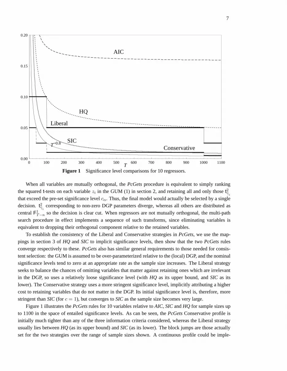
Figure 1 Significance level comparisons for 10 regressors.

When all variables are mutually orthogonal, thePcGetsprocedure is equivalent to simply ranking

the squaredt-tests on each variablezi in the GUM (1) in section 2, and retaining all and only thoset2γi

that exceed the pre-set significance levelcα. Thus, the final model would actually be selected by a single

decision. t2γi

corresponding to non-zero DGP parameters diverge, whereasall others are distributed as

centralF1T−n so the decision is clear cut. When regressors are not mutually orthogonal, the multi-path

search procedure in effect implements a sequence of such transforms, since eliminating variables is

equivalent to dropping their orthogonal component relative to the retained variables.

To establish the consistency of the Liberal and Conservative strategies inPcGets, we use the map-

pings in section 3 ofHQ andSIC to implicit significance levels, then show that the twoPcGetsrules

converge respectively to these.PcGetsalso has similar general requirements to those needed for consis-

tent selection: the GUM is assumed to be over-parameterizedrelative to the (local) DGP, and the nominal

significance levels tend to zero at an appropriate rate as thesample size increases. The Liberal strategy

seeks to balance the chances of omitting variables that matter against retaining ones which are irrelevant

in the DGP, so uses a relatively loose significance level (with HQ as its upper bound, andSIC as its

lower). The Conservative strategy uses a more stringent significance level, implicitly attributing a higher

cost to retaining variables that do not matter in the DGP. Itsinitial significance level is, therefore, more

stringent thanSIC(for c = 1), but converges toSICas the sample size becomes very large.

Figure 1 illustrates thePcGetsrules for 10 variables relative toAIC, SICandHQ for sample sizes up

to 1100 in the space of entailed significance levels. As can beseen, thePcGetsConservative profile is

initially much tighter than any of the three information criteria considered, whereas the Liberal strategy

usually lies betweenHQ (as its upper bound) andSIC (as its lower). The block jumps are those actually

set for the two strategies over the range of sample sizes shown. A continuous profile could be imple-

8

mented with ease, such as that using the nearest selection criterion value, orT−0.8 (also shown, based on

Hendry, 1995, Ch. 13). However, as the two pre-programmed strategies are designed for relatively non-

expert users, it seems preferable to base them more closely on ‘conventional’ significance levels.AIC is

substantially less stringent, particularly at larger sample sizes, so would tend to over-select when there

are many irrelevant candidate variables. However, the Conservative profile is noticeably tighter thanSIC

at small samples, so the next section compares it withSIC. Importantly, while bothSICandHQ deliver

consistent selections, they could differ substantively insmall samples, and it is precisely the intent of the

two PcGetsstrategies to outperform for models and samples of a size relevant to macro-econometrics.

Users ought to carefully evaluate the relative costs of over- versusunder- selection for the problem at

hand before deciding on the nominal significance level, and hence the choice of strategy.

0.00

0.05

0.10

0.15

0.20

0 500 1000 1500 2000 2500 3000 3500 4000 4500 5000T

AIC

HQ

LiberalSIC

T−0.8Conservative

Figure 2 Significance level comparisons for 40 regressors.

Figure 2 shows the corresponding comparisons for40 variables to illustrate the impact of increasing

that dimension, now forT ≤ 5000. Even at such large sample sizes, the implicit significance levels of the

various rules differ substantially. Both these figures holdn fixed asT diverges, albeit at very different

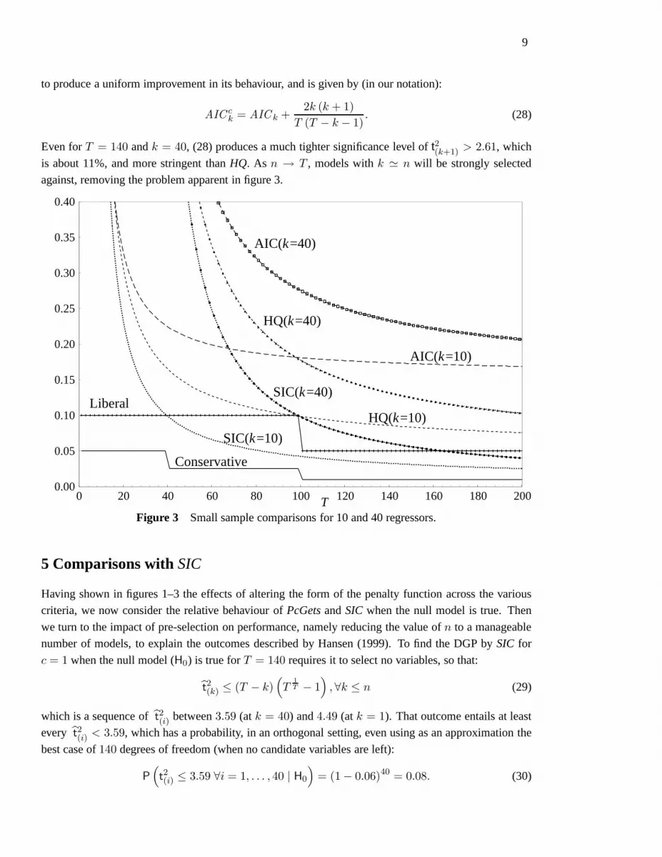
levels. Figure 3 focuses on smaller sample sizes, namelyT ≤ 200, and now compares the two sets

(n = 10 andn = 40), to show the impact of many more variables. The selection rules have increasingly

high levels of significance as the number of candidate variables approaches the sample size (i.e.,n → T ),

which does not seem a desirable feature.3 However, based on Sugiura (1978), Hurvich and Tsai (1989)

derive a non-stochastic correction toAIC that retains asymptotically efficient selection, but corrects its

bias as an estimator of the Kullback–Leibler information discrepancy measure (see e.g., Kullback and

Leibler, 1951), when there are large numbers of parameters relative to the available sample. This appears

3PcGetscan handlen > T , by repeated block searches (see Hendry and Krolzig, 2003c), so maintains relatively tighterlevels.

9

to produce a uniform improvement in its behaviour, and is given by (in our notation):

AICck = AIC k +

2k (k + 1)

T (T − k − 1). (28)

Even forT = 140 andk = 40, (28) produces a much tighter significance level oft2(k+1) > 2.61, which

is about 11%, and more stringent thanHQ. As n → T , models withk ' n will be strongly selected

against, removing the problem apparent in figure 3.

0.00

0.05

0.10

0.15

0.20

0.25

0.30

0.35

0.40

0 20 40 60 80 100 120 140 160 180 200T

AIC(k=10)

HQ(k=10)

AIC(k=40)

HQ(k=40)

SIC(k=40)

SIC(k=10)

Conservative

Liberal

Figure 3 Small sample comparisons for 10 and 40 regressors.

5 Comparisons withSIC

Having shown in figures 1–3 the effects of altering the form ofthe penalty function across the various

criteria, we now consider the relative behaviour ofPcGetsandSIC when the null model is true. Then

we turn to the impact of pre-selection on performance, namely reducing the value ofn to a manageable

number of models, to explain the outcomes described by Hansen (1999). To find the DGP bySIC for

c = 1 when the null model (H0) is true forT = 140 requires it to select no variables, so that:

t2(k) ≤ (T − k)(T

1

T − 1)

,∀k ≤ n (29)

which is a sequence oft2(i) between3.59 (at k = 40) and4.49 (at k = 1). That outcome entails at least

every t2(i) < 3.59, which has a probability, in an orthogonal setting, even using as an approximation the

best case of140 degrees of freedom (when no candidate variables are left):

P(t2(i) ≤ 3.59 ∀i = 1, . . . , 40 | H0

)= (1 − 0.06)40 = 0.08. (30)

10

Thus92% of the timeSICshould retain some irrelevant variable(s).

More formally, let thek mutually independent explanatory variables ordered by their squaredt-values around zero be denoted byτ i so that0 ≤ τ1 ≤ τ2 ≤ · · · ≤ τk < ∞. We wish to compute the

probabilities of exclusion when allk variables are irrelevant, so thet2(i) are distributed as centralF1T−k.

Because theF-statistics are independent, the joint density of the{τ i} is:

gτ1,τ2,...,τk(τ1, τ2, . . . , τ k) = k!

k∏

i=1

g (τ i) ,

whereg (τ i) is the density of a centralF1T−k. For anα% significance level, the probability of correctly

excluding allk variables is:

P (τ i ≤ cα, i = 1, . . . , k | H0)

= P (0 ≤ τ1 ≤ τ2 ≤ · · · ≤ τk ≤ cα)

= k!

∫ cα

0

∫ cα

τ1

· · ·∫ cα

τk−1

k∏

i=1

g (τ i) dτk · · · dτ1

= Gk (cα) (31)

whereG (cα) is the (cumulative) distribution function of theF1T−k distribution. Whenk = 40 with 140

degrees of freedom, (31) yields:

P (τ i ≤ 3.59, i = 1, . . . , 40) = G40 (3.59) = (1 − 0.06)40 = 0.080 (32)

matching (30).

However, since there will be many ‘highly insignificant’ variables in a set of40 irrelevant regres-

sors, the bound oft2(i) < 4.99 is probably the binding one, yielding (at the ‘average’ of120 degrees

of freedom),P(t2(i) < 4.99 ∀i) ' 0.3. Reducing bothT andk need not in fact improve the chances of

correct selection whenk/T rises: for example,T = 80, c = 1 andk = 30 leads to a range between

P(t2(i) ≤ 2.82,∀i = 1, . . . , 30) ' 0.04 andP(t2(i) ≤ 4.45,∀i) ' 0.31. Such probabilities of correctly se-

lecting a null model at relevant sample sizes are too low to provide a useful practical basis. Consequently,

two amendments have been proposed.

The first is reducing the maximum size of model to be considered using ‘pre-selection’ as in (say)

Hansen (1999). He enforces a maximum of10 variables in theSIC formula whenT = 140, despite

n = 40 initially, by sequentially eliminating variables with thesmallestt-values until30 are removed.

However, such a procedure entails thatSIC actually confronts a different problem, namely a penalty

function applied as ifn = 10, so we consider the consequences of that step. If pre-selection did not

matter, then under the null, whenk = 10 with 130 degrees of freedom, (29 deliverst2(10) ≤ 4.67 so:

P (τ i ≤ 4.67, i = 1, . . . , 10) = G10 (4.67) = (0.9675)10 = 0.72. (33)

Using the ‘baseline’F-value of3.59 (from n = 40) in (30) yields:

P(t2(i) ≤ 3.59,∀i = 1, . . . , 10

)= 0.54 (34)

so even allowing for the initial existence of40 variables matters considerably. But the retained variables

are those selected to have the largestt-values out of the whole set ofk = 40 (not justk = 10), so (33)

11

overstates the likely performance of Hansen’s approach. Conversely (30) will understate what happens

after pre-selection, because the very act of alteringn changes the parameters ofSIC, and is not just a

‘numerical implementation’. Hansen (his Table 1) reports aprobability of0.45 for correctly locating the

null model whenc = 1 in his Monte Carlo applied to Hoover–Perez experiments, when excluding the30

variables with the smallestt-values irrespective of their significance.

Formally, the conditional probability of the10 largest squaredt-values being insignificant at the

critical valuec∗α entailed by (29) applied as ifk = 10, given that thek1 = 30 smallest squaredt-values

have been excluded as insignificant is:

P (τ i ≤ c∗α, i = k1 + 1, . . . , k | τ i ≤ c∗α, i = 1, . . . , k1)

=P (0 ≤ τ1 ≤ τ 2 ≤ · · · ≤ τk ≤ c∗α)

P (0 ≤ τ1 ≤ τ2 ≤ · · · ≤ τk1≤ c∗α)

. (35)

The numerator is (31), and the denominator is obtained from the marginal density ofτ1, . . . , τk1which

is:

gτ1,τ2,...,τk1(τ1, τ 2, . . . , τk1

) =k!

(k − k1)!(1 − G (τk1

))k−k1

k1∏

i=1

g (τ i) ,

so:

P (0 ≤ τ1 ≤ τ2 ≤ · · · ≤ τk1≤ c∗α)

=k!

(k − k1)!

∫ cα

0

∫ cα

τ1

· · ·∫ cα

τk1

(1 − G (τk1))k−k1

k1∏

i=1

g (τ i) dτk1· · · dτ1

=

k−k1∑

i=0

k!

i! (k − i)!Gk−i (c∗α) (1 − G (c∗α))i .

The probability of excluding the last10 variables (those with largestt-values) given that we have ex-

cluded the first30 variables, has a denominator:

P (0 ≤ τ1 ≤ τ2 ≤ · · · ≤ τ30 ≤ c∗α)

=

10∑

i=0

40!

i! (40 − i)!G40−i (4.67) (1 − G (4.67))i

=

10∑

i=0

40!

i! (40 − i)!(0.9675)40−i (0.0325)i

' 1.0.

Unsurprisingly, the11th largestt-value is not significant under the null, so from (35):

P (τ i ≤ 4.67, i = 31, . . . , 40 | τ i ≤ 4.67, i = 1, . . . , 30)

=P (0 ≤ τ1 ≤ τ 2 ≤ · · · ≤ τk ≤ 4.67)

P (0 ≤ τ1 ≤ τ2 ≤ · · · ≤ τk1≤ 4.67)

' 0.267

1= 0.267,

which is smaller that0.54 in (34), and smaller than Hansen found by simulation, but much larger than

(32). Pre-selecting out the least significant variables improves the performance ofSIC in finite samples,

12

although it would seem in general preferable to follow thePcGetsapproach of usingF-tests to do so,

rather than arbitrarily exclude a pre-assigned number of regressors, despite the low probability of their

significance under the null. Notice that whenT = 140, k1 = 0 andk = 10, the unconditional value of

F10130 from (25) only needs to be less than5.5 whenc ≥ 1.0, which is virtually certain to occur under the

null, so block tests have advantages here.

A second approach to raising the chances of correctly selecting the null model is to increasec. For

example,c = 2 raises the requiredt2(i) to 7.31 in Hoover–Perez, and hence forn = 40:

P(t2(i) ≤ 7.31,∀i = 1, . . . , 40

)= (1 − 0.0081)40 = 0.73,

which is a dramatic improvement over (30). Hansen’s settingof c = 2 whenn = 10 further raises the

requiredt2(i) to 9.51, and ignoring pre-selection would deliver a97.5% chance of correctly finding a null

model. The actual conditional probability forc = 2 andc∗α = 9.51 is:

P (τ i ≤ 9.51, i = 31, . . . , 40 | τ i ≤ 9.51, i = 1, . . . , 30) = 0.905,

which is much larger than forc = 1 (Hansen reports95% in his Monte Carlo, whereas(1 − 0.0081)10 =

0.92).

Nevertheless, when the null is false, both steps of raisingc and/or statistically or arbitrarily simpli-

fying till 10 variables remain could greatly reduce the probability of retaining relevant regressors with

absolutet-values smaller than2.5, as Hansen notes. This effect does not show up in his analysisof the

Hoover–Perez experiments because the populationt-values are either very large or very small. Moreover,

there are very few relevant variables in the DGPs of those experiments, whereasm > 10 in (5) would

ensure an inconsistent selection.

6 Conclusion

The automatic selection algorithms inPcGetsprovide consistent selection rules likeSIC or HQ, based

on the logic of the behaviour of information criteria, but mapped to significance levels. However, the

asymptotic comfort of consistent selection when the model nests the DGP does not greatly restrict the

choice of strategy in small samples. As shown in figures 1–3, there is a very wide range of implicit

significance levels across the information criteria, and (e.g.) neitherAIC nor HQ seem well designed for

the null-DGP experiments in Hoover and Perez (1999): evenSIC struggles. In finite samples,PcGets

both ensures a congruent model and can out-perform in important special cases (such as a null DGP)

without ad hocadjustments. Indeed, depending on the state of nature,PcGetscan have a higher proba-

bility of finding the DGP starting from a highly over-parameterized GUM using the Liberal strategy, than

commencing from the DGP and selecting by the Conservative strategy (see Hendry and Krolzig, 2003b).

Such a finding would have seemed astonishing in the aftermathof Lovell (1983), and both shows the

progress achieved and serves to emphasize the importance ofthe choice of strategy for the underlying

selection problem.

Four other conclusions emerge from this analysis. First, pre-selection can help locate the DGP by

altering the ‘parameters’ entered intoSICcalculations, specifically the apparent degrees of freedomand

the implicitly requiredt-value. PcGetsemploys a statistical ‘pre-selection’ first stage based on block

sequential tests, but with loose significance levels, to tryan ensure that relevant variables are unlikely

13

to be eliminated. This greatly improves its performance when the null is true, but also does so more

generally. The findings reported in Hansen (1999) for other cases suggest that a similar result holds in

finite samples forSIC. Secondly, the trade-off between retaining irrelevant andlosing relevant variables

remains for information criteria, and is determined by the choice of c in SIC implicitly altering the

significance level. In problems with manyt-values around 2 or 3, high values ofc will be detrimental,

and almost surely not compensated by benefits achieved when the DGP is null. Thirdly,SIC does not

address the difficulty that the initial model specification may not be adequate to characterize the data,

andSICwill select a ‘best’ representation without evidence on howpoor it may be. In contrast,PcGets

commences by testing for congruency: perversely, in Monte Carlo experiments conducted to date, where

the DGP is a special case of the general model, such testing lowers the relative success rate ofPcGets.

Finally, the arbitrary specification of an upper bound onn is both counter to the spirit ofSIC, and

would deliver adverse findings in any setting wheren was set lower than the numberm of relevant DGP

variables.

We have not explored a strategy coinciding withAICck but intend to do so, to allow an option for

users interested in asymptotically efficient selection.

References

Akaike, H. (1969). Fitting autoregressive models for prediction. Annals of the Institute of Statistical

Mathematics, 21, 243–247.

Akaike, H. (1973). Information theory and an extension of the maximum likelihood principle. In Petrov,

B. N., and Csaki, F. (eds.),Second International Symposion on Information Theory, pp. 267–281.

Budapest: Akademia Kiado.

Atkinson, A. C. (1981). Likelihood ratios, posterior odds and information criteria.Journal of Economet-

rics, 16(1), 15–20.

Campos, J., Ericsson, N. R., and Hendry, D. F. (2003). Editors’ introduction. In Campos, J., Ericsson,

N. R., and Hendry, D. F. (eds.),Readings on General-to-Specific Modeling. Cheltenham: Edward

Elgar. Forthcoming.

Doornik, J. A. (1999).Object-Oriented Matrix Programming using Ox. London: Timberlake Consultants

Press. 3rd edition.

Hannan, E. J., and Quinn, B. G. (1979). The determination of the order of an autoregression.Journal of

the Royal Statistical Society, B, 41, 190–195.

Hansen, B. E. (1999). Discussion of ‘Data mining reconsidered’. Econometrics Journal, 2, 26–40.

Hendry, D. F. (1995).Dynamic Econometrics. Oxford: Oxford University Press.

Hendry, D. F., and Krolzig, H.-M. (2001).Automatic Econometric Model Selection. London: Timberlake

Consultants Press.

Hendry, D. F., and Krolzig, H.-M. (2003a). New developmentsin automatic general-to-specific mod-

elling. In Stigum, B. P. (ed.),Econometrics and the Philosophy of Economics, pp. 379–419.

Princeton: Princeton University Press.

Hendry, D. F., and Krolzig, H.-M. (2003b). The properties ofautomatic Gets modelling. Unpublished

paper, Economics Department, Oxford University.

14

Hendry, D. F., and Krolzig, H.-M. (2003c). Model selection with more variables than observations.

Unpublished paper, Economics Department, Oxford University.

Hoover, K. D., and Perez, S. J. (1999). Data mining reconsidered: Encompassing and the general-to-

specific approach to specification search.Econometrics Journal, 2, 167–191.

Hurvich, C. M., and Tsai, C.-L. (1989). Regression and time series model selection in small samples.

Biometrika, 76, 297–307.

Krolzig, H.-M., and Hendry, D. F. (2001). Computer automation of general-to-specific model selection

procedures.Journal of Economic Dynamics and Control, 25, 831–866.

Kullback, S., and Leibler, R. A. (1951). On information and sufficiency. Annals of Mathematical Statis-

tics, 22, 79–86.

Lovell, M. C. (1983). Data mining.Review of Economics and Statistics, 65, 1–12.

Phillips, P. C. B. (1994). Bayes models and forecasts of Australian macroeconomic time series. In

Hargreaves, C. (ed.),Non-stationary Time-Series Analyses and Cointegration. Oxford: Oxford

University Press.

Phillips, P. C. B. (1995). Automated forecasts of Asia-Pacific economic activity.Asia-Pacific Economic

Review, 1, 92–102.

Phillips, P. C. B. (1996). Econometric model determination. Econometrica, 64, 763–812.

Phillips, P. C. B., and Ploberger, W. (1995). An asymptotic theory of Bayesian inference for time series.

Econometrica, 63, 381–412.

Rissanen, J. (1978). Modeling by shortest data description. Automatica, 14, 465–471.

Robinson, P. M. (2003). Denis Sargan: Some perspectives.Econometric Theory, 19, 481–494.

Sargan, J. D. (1975). Asymptotic theory and large models.International Economic Review, 16, 75–91.

Schwarz, G. (1978). Estimating the dimension of a model.Annals of Statistics, 6, 461–464.

Shibata, R. (1980). Asymptotically efficient selection of the order of the model for estimating parameters

of a linear process.Annals of Statistics, 8, 147–164.

Sober, E. (2003). Instrumentalism, parsimony, and the Akaike framework. Unpublished paper, Depart-

ment of Philosophy, University of Wisconsin, Madison.

Sugiura, N. (1978). Further analysis of the data by Akaike’sinformation criterion and the finite correc-

tions. Communications in Statistics, A78, 13–26.

Theil, H. (1961). Economic Forecasts and Policy,2nd edn. Amsterdam: North-Holland Publishing

Company.

White, H. (1990). A consistent model selection. In Granger,C. W. J. (ed.),Modelling Economic Series,

pp. 369–383. Oxford: Clarendon Press.